CHMAS: A Coupled Hierarchical Framework for Multi-Agent Reinforcement Learning

Dongming Wang, Jie Xu, Yanyu Zhang, and Wei Ren This work was supported by the National Science Foundation under Grant ECCS-2129949.The authors are with the Department of Electrical and Computer Engineering, University of California, Riverside, CA 92521, USA. {wdong025, jxu150, yzhan831, wei.ren}@ucr.edu.

Abstract

Multi-agent reinforcement learning (MARL) systems face fundamental challenges in balancing global coordination with local execution across different temporal scales. This paper introduces the Coupled Hierarchical Multi-Agent System (CHMAS), a novel framework that decomposes multi-agent decision-making into centralized strategic planning and distributed tactical execution with bidirectional information flow. The strategic layer integrates all agents’ states with an exclusive global environmental state to generate guidance actions every $T$ timesteps, while tactical agents execute distributed policies augmented by strategic guidance and local neighborhood observations. Unlike existing hierarchical approaches with unidirectional control, CHMAS establishes a feedback mechanism where accumulated tactical rewards influence strategic objectives through a coupling coefficient $\lambda$ , ensuring strategic plans remain grounded in tactical feasibility. To address the non-stationarity inherent in hierarchical learning, we propose an asynchronous update protocol where strategic parameters update every $N_{f}$ tactical episodes, allowing tactical policies to converge to quasi-stationary points between strategic changes. We present both a general bi-level formulation capturing full system dynamics and a tractable additive approximation enabling rigorous analysis. Theoretical analysis proves that this asynchronous scheme achieves $\mathcal{O}(\log K/\sqrt{K})$ convergence for the strategic layer after $K$ strategic updates under standard assumptions. Experimental validation in a multi-agent foraging domain demonstrates successful learning of spatially partitioned exploration strategies, with both layers converging stably despite hierarchical coupling.

I INTRODUCTION

Multi-agent reinforcement learning (MARL) has emerged as a fundamental paradigm for autonomous coordination in complex environments, with applications spanning robotics [12], traffic management [22], and resource allocation [15]. Despite significant progress, real-world deployment faces a critical challenge: coordinating distributed agents across multiple temporal and spatial scales while maintaining computational tractability.

The curse of dimensionality renders purely centralized approaches intractable. For $N$ agents with state spaces $\mathcal{S}_{i}$ and action spaces $\mathcal{A}_{i}$ , the joint space grows as $O(\prod_{i=1}^{N}|\mathcal{S}_{i}|\cdot|\mathcal{A}_{i}|)$ [23]. While distributed methods address scalability through local decision-making [24], they sacrifice coordination quality for long-horizon objectives. Traditional approaches like QMIX [16] and MADDPG [8] leverage centralized training with decentralized execution, but assume all agents access relevant global information during training, which often fails in practice due to partial observability and communication constraints [5].

Furthermore, multi-agent systems inherently operate across multiple temporal scales. Strategic decisions (formation control, task allocation) require global information including environmental states inaccessible to individual agents, operating on extended timescales. Tactical responses (collision avoidance, local adaptation) demand rapid reactions based on immediate observations. While hierarchical reinforcement learning offers a natural framework for multi-scale decision-making [19, 2], existing hierarchical MARL approaches [14, 21] employ unidirectional control where high-level policies dictate low-level actions, missing opportunities for tactical feedback to inform strategic planning.

The interaction between hierarchical levels creates complex learning dynamics. Strategic changes fundamentally alter the environment perceived by tactical agents, violating stationarity assumptions [5]. Conversely, evolving tactical policies change execution characteristics that strategic planners rely upon. Previous hierarchical MARL work [7, 9] addresses this through reward engineering or option learning but requires domain expertise and often fails to generalize.

This paper introduces CHMAS, which addresses these limitations through bidirectional coupling between strategic and tactical layers at different temporal scales. The strategic level maintains centralized access to both agents’ states and an exclusive global environmental state $\mathcal{S}^{\text{env}}$ capturing system-wide properties essential for coordination. Strategic guidance, generated every $T$ timesteps, broadcasts to tactical agents who execute distributed policies based on augmented local observations. Tactical rewards accumulate and influence strategic objectives through coupling coefficient $\lambda$ , creating feedback that grounds strategic planning in tactical realities. An asynchronous protocol with strategic updates every $N_{f}$ tactical episodes manages non-stationary dynamics, allowing tactical convergence between strategic changes.

Our contributions are threefold. First, we formalize the hierarchical MARL problem with bidirectional coupling and information asymmetry, providing both a general bi-level formulation and tractable additive approximation. Second, we develop the Asynchronous Hierarchical Policy Gradient (AHPG) algorithm managing non-stationarity through temporal separation while maintaining $\mathcal{O}(\log K/\sqrt{K})$ convergence guarantees for the strategic layer. Third, we validate the framework empirically, demonstrating stable bidirectional learning in a cooperative multi-agent foraging task.

II PRELIMINARIES

We consider a cooperative multi-agent system with $N$ agents operating in a shared environment. The system employs a hierarchical architecture with a strategic layer that accesses global information at low temporal frequency and a tactical layer that operates distributedly at high frequency using only local information.

II-A Multi-Agent Communication Graph

The tactical agents interact through a time-invariant communication graph $\mathcal{G}=(\mathcal{V},\mathcal{E})$ where $\mathcal{V}=\{1,2,\ldots,N\}$ represents the agent set and $\mathcal{E}\subseteq\mathcal{V}\times\mathcal{V}$ denotes the edge set [13, 10]. For each agent $i$ , the neighborhood $\mathcal{N}_{i}=\{j\in\mathcal{V}:(i,j)\in\mathcal{E}\}$ is the set of agents that can directly communicate with agent $i$ . This graph constrains information flow at the tactical level, ensuring distributed execution remains scalable.

II-B Strategic MDP

Definition 1 (Strategic MDP)

The strategic layer evolves as $\mathcal{M}^{\text{str}}=(\mathcal{S}^{\text{str}},\mathcal{A}^{\text{str}},P^{\text{str}},R^{\text{str}},\gamma_{\text{str}})$ , where: (i) the state $\mathcal{S}^{\text{str}}=\mathcal{S}^{\text{env}}\times\prod_{i=1}^{N}\mathcal{S}_{i}$ combines the exclusive global environmental state $\mathcal{S}^{\text{env}}$ (resource distributions, global objectives) with all agent states, so that at epoch $k$ the strategic state is $s^{\text{str}}_{k}=(s^{\text{env}}_{k},s_{1,k},\ldots,s_{N,k})$ ; (ii) actions $\mathcal{A}^{\text{str}}=\prod_{i=1}^{N}\mathcal{A}^{\text{str}}_{i}$ provide personalized guidance $a^{\text{str}}_{i,k}$ to each agent, persisting for the interval $[kT,(k+1)T)$ ; and (iii) the reward integrates global objectives with tactical feedback:

R^{\text{str}}(s^{\text{str}}_{k},\mathbf{a}^{\text{str}}_{k})=R^{\text{global}}(s^{\text{env}}_{k},\mathbf{a}^{\text{str}}_{k})+\lambda\sum_{t=kT}^{(k+1)T-1}\sum_{i=1}^{N}r^{\text{tac}}_{i,t},

(1)

where $\lambda\in[0,1]$ controls the influence of tactical execution quality on strategic evaluation.

The strategic policy $\pi^{\text{str}}:\mathcal{S}^{\text{str}}\rightarrow\mathcal{P}(\mathcal{A}^{\text{str}})$ maps complete state observations to guidance distributions, encoding high-level coordination logic that individual agents cannot compute from local information alone.

II-C Tactical Multi-Agent MDP

Definition 2 (Tactical MAMDP)

Given fixed strategic guidance $\mathbf{a}^{\text{str}}_{k}$ , the tactical layer evolves as $\mathcal{M}^{\text{tac}}=(\{\mathcal{S}_{i}\},\{\mathcal{O}^{\text{tac}}_{i}\},\{\mathcal{A}^{\text{tac}}_{i}\},P^{\text{tac}},\{R^{\text{tac}}_{i}\},\gamma_{\text{tac}})$ , where: (i) each agent $i$ observes

o^{\text{tac}}_{i,t}=\phi_{i}(s_{i,t},\{s_{j,t}\}_{j\in\mathcal{N}_{i}},a^{\text{str}}_{i,k})\in\mathcal{O}^{\text{tac}}_{i},

(2)

combining local state, neighbor states, and strategic guidance ( $k=\lfloor t/T\rfloor$ ); (ii) the joint transition factorizes over the communication graph: $P^{\text{tac}}(\mathbf{s}_{t+1}|\mathbf{s}_{t},\mathbf{a}^{\text{tac}}_{t})=\prod_{i=1}^{N}P_{i}(s_{i,t+1}|s_{i,t},\{s_{j,t},a^{\text{tac}}_{j,t}\}_{j\in\mathcal{N}_{i}\cup\{i\}})$ , maintaining tractability as $N$ grows [23]; and (iii) the per-agent reward

R^{\text{tac}}_{i}(s_{i,t},a^{\text{tac}}_{i,t},\{s_{j,t},a^{\text{tac}}_{j,t}\}_{j\in\mathcal{N}_{i}},a^{\text{str}}_{i,k})

(3)

enables local optimization and neighbor coordination while incorporating strategic objectives.

II-D Bidirectional Coupling

Unlike traditional top-down hierarchies [14], CHMAS establishes feedback in both directions. Downward coupling (strategic $\to$ tactical): guidance $a^{\text{str}}_{i,k}$ shapes tactical behavior through observation augmentation (2), reward modulation (3), and temporal persistence over $T$ timesteps. Upward coupling (tactical $\to$ strategic): accumulated rewards $R^{\text{tac,cum}}_{k}=\sum_{t=kT}^{(k+1)T-1}\sum_{i=1}^{N}r^{\text{tac}}_{i,t}$ influence strategic rewards via $\lambda$ in (1), so that strategic decisions account for tactical feasibility. Setting $\lambda=0$ recovers a purely top-down hierarchy. The framework maintains asymmetric information access: the strategic layer observes complete state $s^{\text{str}}_{k}$ while tactical agents access only $\mathcal{N}_{i}$ , with strategic guidance serving as an information bottleneck [20].

III PROBLEM FORMULATION

III-A General Coupled Formulation

The bidirectional coupling creates a bi-level optimization structure [4, 18]. The strategic objective:

J^{\text{str}}(\theta^{\text{str}}|\{\theta^{\text{tac}}_{i}\})=\mathbb{E}\!\left[\sum_{k=0}^{\infty}\gamma^{k}_{\text{str}}R^{\text{str}}(s^{\text{str}}_{k},\mathbf{a}^{\text{str}}_{k})\right]

(4)

depends on tactical policies through (1). Each tactical objective:

J^{\text{tac}}_{i}(\theta^{\text{tac}}_{i}|\theta^{\text{str}})=\mathbb{E}\!\left[\sum_{t=0}^{\infty}\gamma^{t}_{\text{tac}}r^{\text{tac}}_{i,t}\right]

(5)

depends on strategic parameters through (2) and (3).

Definition 3 (Coupled Hierarchical Problem)

The coupled optimization problem is the bi-level program:

	$\displaystyle\max_{\theta^{\text{str}}}\quad$	$\displaystyle J^{\text{str}}(\theta^{\text{str}}\|\{\theta^{\text{tac}*}_{i}(\theta^{\text{str}})\})$
	s.t.	$\displaystyle\theta^{\text{tac}*}_{i}(\theta^{\text{str}})=\arg\max_{\theta^{\text{tac}}_{i}}J^{\text{tac}}_{i}(\theta^{\text{tac}}_{i}\|\theta^{\text{str}}),\quad\forall i\in\mathcal{V},$

where the strategic optimization accounts for tactical best responses.

Remark 1

We operate in the cooperative MARL setting where agents share a common team objective. Accordingly, the per-agent best responses $\theta^{\text{tac}*}_{i}$ are aligned with the joint team optimum, and no equilibrium-seeking across agents is required at the tactical level [23].

This Stackelberg structure is computationally intractable in general [6], motivating the approximation below.

III-B Additive Approximation for Tractable Optimization

Definition 4 (Additive Hierarchical Problem)

Under the additive approximation, the global objective is:

J^{\text{global}}(\theta^{\text{str}},\{\theta^{\text{tac}}_{i}\})=J^{\text{str}}(\theta^{\text{str}})+\sum_{i=1}^{N}J^{\text{tac}}_{i}(\theta^{\text{tac}}_{i}),

(6)

where each term is evaluated with fixed parameters of the other layer.

Remark 2

Equation (6) is an approximation of the true coupled objective: the cross-layer dependencies in (4)–(5) are not eliminated but handled implicitly through the asynchronous update schedule. The approximation error is controlled by the tactical optimality gap $\delta_{k}$ which will be defined in Assumption 2 at each epoch, which vanishes as learning progresses.

The separable gradient structure,

\nabla_{\theta}J^{\text{global}}=\bigl[\nabla_{\theta^{\text{str}}}J^{\text{str}},\;\nabla_{\theta^{\text{tac}}}J^{\text{tac}}\bigr]^{T},

(7)

allows updates to be treated as coordinate steps in the joint parameter space, enabling rigorous convergence analysis via two-timescale stochastic approximation [3, 11].

IV ASYNCHRONOUS LEARNING ALGORITHM

IV-A Algorithm Design Principles

AHPG leverages three principles for stable hierarchical learning.

Temporal separation. Strategic decisions occur every $T$ timesteps and persist throughout the interval. Strategic parameters follow a decaying step size schedule $\eta^{\text{str}}_{k}=\alpha/\sqrt{k}$ and update only every $N_{f}$ tactical episodes, operating at a slower effective timescale than tactical learning. This allows tactical policies to converge to near-optimal responses between strategic changes, transforming the non-stationary hierarchical problem into alternating stationary subproblems.

Structured information flow. Downward flow provides coordination signals through strategic guidance without requiring centralized control at each timestep. Upward flow aggregates tactical performance $R^{\text{tac}}_{k}=\sum_{t,i}r^{\text{tac}}_{i,t}$ into strategic rewards, keeping high-level plans grounded in execution realities. The strategic layer maintains exclusive access to $s^{\text{env}}_{k}$ , preserving the information asymmetry that enables scalable distributed execution.

Distributed tactical learning. Each tactical agent maintains its own policy $\pi^{\text{tac}}_{i}$ and experience buffer $\mathcal{D}^{\text{tac}}_{i}$ , updating parameters using only local gradients without inter-agent communication during learning, so that tactical computation scales linearly with $N$ .

IV-B Algorithm Specification

Algorithm 1 presents the complete AHPG procedure. Strategic guidance is generated at the start of each new strategic epoch (every $N_{f}$ episodes), and strategic parameters are updated at the end of each epoch using the accumulated tactical performance. Tactical parameters update every episode.

Algorithm 1 Asynchronous Hierarchical Policy Gradient (AHPG)

0: Initial parameters

\theta^{\text{str}}_{1}

\{\theta^{\text{tac}}_{i,0}\}

0: Hyperparameters

T

N_{f}

\alpha

\eta^{\text{tac}}

\lambda

c

1: Initialize episode counter

e\leftarrow 0

, strategic epoch

k\leftarrow 1

2: for episode

e=1,2,\ldots

3: // Strategic Planning Phase

4: if

e\bmod N_{f}=1

then

5: Observe full state

s^{\text{str}}_{k}=(s^{\text{env}}_{k},\mathbf{s}_{k})

6: Generate

\mathbf{a}^{\text{str}}_{k}\sim\pi^{\text{str}}(s^{\text{str}}_{k};\,\theta^{\text{str}}_{k})

7: Broadcast

a^{\text{str}}_{i,k}

to each agent

i

8: end if

9: // Tactical Execution Phase

10: for

t=0

T-1

11: for agent

i\in\mathcal{V}

in parallel do

12:

o^{\text{tac}}_{i,t}=\phi_{i}(s_{i,t},\{s_{j,t}\}_{j\in\mathcal{N}_{i}},a^{\text{str}}_{i,k})

13:

a^{\text{tac}}_{i,t}\sim\pi^{\text{tac}}_{i}(o^{\text{tac}}_{i,t};\,\theta^{\text{tac}}_{i,e})

14: Store

(o^{\text{tac}}_{i,t},a^{\text{tac}}_{i,t},r^{\text{tac}}_{i,t})

\mathcal{D}^{\text{tac}}_{i}

15: end for

16: end for

17: // Tactical Policy Update

18: for agent

i\in\mathcal{V}

in parallel do

19:

g^{\text{tac}}_{i}=\nabla_{\theta^{\text{tac}}_{i}}J^{\text{tac}}_{i}

using

\mathcal{D}^{\text{tac}}_{i}

20:

\theta^{\text{tac}}_{i,e+1}=\theta^{\text{tac}}_{i,e}+\eta^{\text{tac}}g^{\text{tac}}_{i}

21: end for

22: // Strategic Update

23: if

e\bmod N_{f}=0

then

24:

R^{\text{tac}}_{k}=\sum_{t=kT}^{(k+1)T-1}\sum_{i=1}^{N}r^{\text{tac}}_{i,t}

25:

r^{\text{str}}_{k}=R^{\text{global}}(s^{\text{env}}_{k},\mathbf{a}^{\text{str}}_{k})+\lambda R^{\text{tac}}_{k}

26:

g^{\text{str}}=\nabla_{\theta^{\text{str}}}J^{\text{str}}

using

\mathcal{D}^{\text{str}}

27:

\theta^{\text{str}}_{k+1}=\theta^{\text{str}}_{k}+(\alpha/\sqrt{k})\,g^{\text{str}}

28:

k\leftarrow k+1

29: end if

30: end for

During the $N_{f}$ episodes between strategic updates, tactical agents operate in a stationary environment with fixed guidance, converging toward near-optimal policies. This ensures strategic updates observe stable tactical performance that accurately estimates the tactical contribution to strategic rewards.

For learning components, the strategic layer employs centralized policy gradient algorithms (e.g., PPO [17]) leveraging complete state access, while tactical agents use distributed policy gradient or actor-critic variants operating on local observations. The framework naturally extends to continuous control through continuous guidance vectors and to partially observable settings through recurrent policies.

V CONVERGENCE ANALYSIS

We establish convergence for AHPG under the additive approximation $J^{\text{global}}(\theta)=J^{\text{str}}(\theta^{\text{str}})+\sum_{i=1}^{N}J^{\text{tac}}_{i}(\theta^{\text{tac}}_{i})$ .

Assumption 1

1.

Smoothness: $J^{\text{str}}$ and each $J^{\text{tac}}_{i}$ are $L$ -smooth with $L$ -Lipschitz gradients.
2.

Boundedness: $J^{\text{str}}\leq J^{\text{str}*}$ and $J^{\text{tac}}_{i}\leq J^{\text{tac}*}_{i}$ for all $i$ .
3.

Bounded variance: Stochastic gradient estimates satisfy $\mathbb{E}[\|g^{\text{str}}_{k}-\nabla J^{\text{str}}_{k}\|^{2}]\leq\sigma^{2}_{\text{str}}$ and $\mathbb{E}[\|g^{\text{tac}}_{i,e}-\nabla J^{\text{tac}}_{i}\|^{2}]\leq\sigma^{2}_{\text{tac}}$ .
4.

Biased strategic gradient: $\mathbb{E}[g^{\text{str}}_{k}\mid\theta^{\text{str}}_{k}]=\nabla J^{\text{str}}(\theta^{\text{str}}_{k})+b_{k}$ , where $b_{k}$ captures the error from evaluating strategic gradients with non-converged tactical parameters.

Assumption 2

1.

PL condition: Each $J^{\text{tac}}_{i}$ satisfies the $\mu$ -PL inequality: $\|\nabla J^{\text{tac}}_{i}(\theta)\|^{2}\geq 2\mu(J^{\text{tac}*}_{i}-J^{\text{tac}}_{i}(\theta))$ .
2.

Warm-start: At the beginning of each strategic epoch $k$ , tactical agents are initialized from the converged state of the previous epoch. The initial optimality gap satisfies $\mathbb{E}[J^{\text{tac}*}_{i}-J^{\text{tac}}_{i}(\theta^{\text{tac}}_{i,kN_{f}})]\leq\delta_{k}$ , where $\delta_{k}=\mathcal{O}(\eta^{\text{str}}_{k})=\mathcal{O}(1/\sqrt{k})$ , reflecting the magnitude of the strategic parameter change between successive epochs.
3.

Round-robin updates: Within each tactical phase, agents update sequentially with others’ parameters held fixed, so that the PL condition applies to each per-agent landscape independently.

Remark 3

The PL condition in Assumption 2 holds for log-linear (softmax) policies in tabular settings [1] and locally for over-parameterized neural networks near stationary points. The round-robin assumption is a standard device to decouple per-agent landscapes; it can be relaxed to simultaneous updates at the cost of a more involved coupling analysis.

Assumption 3 (Coupling structure)

The strategic gradient is $L_{b}$ -Lipschitz in the tactical parameters:

\|\nabla J^{\text{str}}(\theta^{\text{str}},\boldsymbol{\theta}^{\text{tac}})-\nabla J^{\text{str}}(\theta^{\text{str}},\boldsymbol{\theta}^{\text{tac}*})\|\leq L_{b}\|\boldsymbol{\theta}^{\text{tac}}-\boldsymbol{\theta}^{\text{tac}*}\|.

Theorem 1 (AHPG Convergence)

Under Assumptions 1–3, with $\eta^{\text{str}}_{k}=\alpha/\sqrt{k}$ where $\alpha\leq 1/(8L)$ , $\eta^{\text{tac}}=\beta/\sqrt{K}$ where $\beta<1/(2L)$ , and $N_{f}=c\sqrt{K}$ for a constant $c>0$ , after $K$ strategic updates AHPG achieves:

\min_{k\in\{1,\ldots,K\}}\mathbb{E}[\|\nabla J^{\text{str}}(\theta^{\text{str}}_{k})\|^{2}]=\mathcal{O}\!\left(\frac{\log K}{\sqrt{K}}\right),

\frac{1}{KN_{f}}\sum_{k=1}^{K}\sum_{e=kN_{f}}^{(k+1)N_{f}-1}\sum_{i=1}^{N}\mathbb{E}[\|\nabla J^{\text{tac}}_{i}(\theta^{\text{tac}}_{i,e})\|^{2}]=\mathcal{O}\!\left(\frac{1}{\sqrt{K}}\right).

Proof:

Strategic layer. By $L$ -smoothness of $J^{\text{str}}$ and the update $\theta^{\text{str}}_{k+1}=\theta^{\text{str}}_{k}+\eta^{\text{str}}_{k}g^{\text{str}}_{k}$ :

J^{\text{str}}_{k+1}\geq J^{\text{str}}_{k}+\eta^{\text{str}}_{k}\langle\nabla J^{\text{str}}_{k},\,g^{\text{str}}_{k}\rangle-\tfrac{L}{2}(\eta^{\text{str}}_{k})^{2}\|g^{\text{str}}_{k}\|^{2}.

Taking expectation with $\mathbb{E}[g^{\text{str}}_{k}]=\nabla J^{\text{str}}_{k}+b_{k}$ , we bound the two terms. For the inner product, applying Young’s inequality $\langle a,b\rangle\geq-\tfrac{1}{4}\|a\|^{2}-\|b\|^{2}$ :

\mathbb{E}[\langle\nabla J^{\text{str}}_{k},g^{\text{str}}_{k}\rangle]\geq\tfrac{3}{4}\|\nabla J^{\text{str}}_{k}\|^{2}-\|b_{k}\|^{2}.

For the squared norm, using $\mathbb{E}[\|g^{\text{str}}_{k}\|^{2}]\leq\|\nabla J^{\text{str}}_{k}+b_{k}\|^{2}+\sigma^{2}_{\text{str}}\leq 2\|\nabla J^{\text{str}}_{k}\|^{2}+2\|b_{k}\|^{2}+\sigma^{2}_{\text{str}}$ :

	$\displaystyle\mathbb{E}[J^{\text{str}}_{k+1}]$	$\displaystyle\geq J^{\text{str}}_{k}+\!\left(\tfrac{3}{4}\eta^{\text{str}}_{k}-L(\eta^{\text{str}}_{k})^{2}\right)\\|\nabla J^{\text{str}}_{k}\\|^{2}$
		$\displaystyle\quad-\!\left(\eta^{\text{str}}_{k}+L(\eta^{\text{str}}_{k})^{2}\right)\\|b_{k}\\|^{2}-\tfrac{L}{2}(\eta^{\text{str}}_{k})^{2}\sigma^{2}_{\text{str}}.$

Since $\eta^{\text{str}}_{k}\leq 1/(8L)$ , we have $L(\eta^{\text{str}}_{k})^{2}\leq\eta^{\text{str}}_{k}/8$ , so $\tfrac{3}{4}\eta^{\text{str}}_{k}-L(\eta^{\text{str}}_{k})^{2}\geq\tfrac{5}{8}\eta^{\text{str}}_{k}\geq\tfrac{1}{8}\eta^{\text{str}}_{k}$ and $\eta^{\text{str}}_{k}+L(\eta^{\text{str}}_{k})^{2}\leq\tfrac{9}{8}\eta^{\text{str}}_{k}\leq 2\eta^{\text{str}}_{k}$ . Rearranging and telescoping over $k=1,\ldots,K$ :

	$\displaystyle\frac{1}{8}\sum_{k=1}^{K}\eta^{\text{str}}_{k}\mathbb{E}[\\|\nabla J^{\text{str}}_{k}\\|^{2}]$	$\displaystyle\leq\Delta J^{\text{str}}+2\sum_{k=1}^{K}\eta^{\text{str}}_{k}\\|b_{k}\\|^{2}$
		$\displaystyle\quad+\frac{L\sigma^{2}_{\text{str}}}{2}\sum_{k=1}^{K}(\eta^{\text{str}}_{k})^{2},$		(8)

where $\Delta J^{\text{str}}=J^{\text{str}*}-J^{\text{str}}_{1}$ .

Bias bound. By Assumption 3, $\|b_{k}\|^{2}\leq L_{b}^{2}\|\boldsymbol{\theta}^{\text{tac}}_{(k+1)N_{f}}-\boldsymbol{\theta}^{\text{tac}*}\|^{2}$ . Running $N_{f}=c\sqrt{K}$ SGD steps under the PL condition (Assumption 2) with step size $\beta/\sqrt{K}$ and warm-start gap $\delta_{k}$ yields contraction factor $\rho=(1-2\mu\beta/\sqrt{K})^{c\sqrt{K}}\to e^{-2\mu\beta c}<1$ , so the residual tactical deviation satisfies $\|b_{k}\|^{2}=\mathcal{O}(\delta_{k}+1/\sqrt{K})=\mathcal{O}(1/\sqrt{k})$ .

Completing the strategic bound. With $\eta^{\text{str}}_{k}=\alpha/\sqrt{k}$ :

	$\displaystyle\sum_{k=1}^{K}\eta^{\text{str}}_{k}\\|b_{k}\\|^{2}$	$\displaystyle=\mathcal{O}\!\left(\alpha\sum_{k=1}^{K}\tfrac{1}{\sqrt{k}}\cdot\tfrac{1}{\sqrt{k}}\right)=\mathcal{O}(\log K),$
	$\displaystyle\sum_{k=1}^{K}(\eta^{\text{str}}_{k})^{2}$	$\displaystyle=\alpha^{2}\sum_{k=1}^{K}\tfrac{1}{k}=\mathcal{O}(\log K).$

Dividing (V) by $\sum_{k=1}^{K}\eta^{\text{str}}_{k}=\mathcal{O}(\alpha\sqrt{K})$ gives $\min_{k}\mathbb{E}[\|\nabla J^{\text{str}}_{k}\|^{2}]=\mathcal{O}(\log K/\sqrt{K})$ .

Tactical layer. Within epoch $k$ , $\theta^{\text{str}}_{k}$ is fixed, so $J^{\text{tac}}_{i}$ is stationary. Standard SGD under the $\mu$ -PL condition over $N_{f}$ steps gives per-epoch average gradient norm $\mathcal{O}(\delta_{k}+1/\sqrt{K})$ . Averaging over $K$ epochs and using $K^{-1}\sum_{k=1}^{K}\delta_{k}=K^{-1}\sum_{k=1}^{K}\mathcal{O}(k^{-1/2})=\mathcal{O}(K^{-1/2})$ , the overall tactical average is $\mathcal{O}(1/\sqrt{K})$ , completing the proof. ∎

Remark 4

Theorem 1 is established for policy gradient implementations. The DQN-based experiments in Section VI serve as an empirical proof of concept; extending the convergence analysis to Q-learning variants is left for future work.

VI EXPERIMENTAL VALIDATION

VI-A Experiment Setting

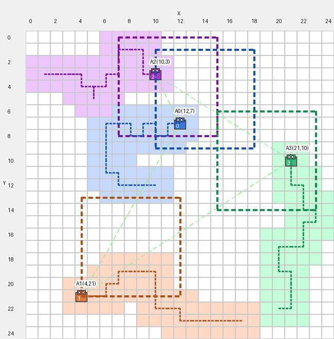
We evaluate CHMAS on a 25 $\times$ 25 GridWorld environment with $N=4$ agents performing cooperative foraging, instantiating the key features of hierarchical multi-agent coordination: information asymmetry, temporal abstraction, and bidirectional coupling.

Refer to caption — Figure 1: The 25 $\times$ 25 GridWorld environment. Four agents (A0-blue, A1-orange, A2-purple, A3-green) operate within their assigned 9 $\times$ 9 regions (dashed boxes) determined by strategic guidance. Colored areas indicate visited cells tracked in the global state $s^{\text{env}}$ , while agents pursue local resources (red apple).

The global environmental state $s^{\text{env}}\in\{0,1\}^{625}$ tracks cell visitation, representing system-wide coverage that individual agents cannot observe. The strategic layer accesses the complete state $s^{\text{str}}=(s^{\text{env}},s_{1},s_{2},s_{3},s_{4})$ , while each tactical agent $i$ observes only local information $o^{\text{tac}}_{i}\in\mathbb{R}^{20}$ comprising its position, nearby resources, and strategic guidance.

Strategic actions assign each agent a 9 $\times$ 9 region center $a^{\text{str}}_{i}=(g^{x}_{i},g^{y}_{i})\in[4,20]^{2}$ at the start of each epoch ( $T=5$ timesteps). Tactical agents select discrete actions $a^{\text{tac}}_{i}\in\{0,1,2,3,4,5\}$ (movement, collection, wait).

The reward structure implements bidirectional coupling: tactical agents receive $r^{\text{tac}}_{i,t}=r^{\text{collect}}_{i,t}-0.01-0.01\cdot\mathbf{1}[\text{outside region}]$ , while the strategic layer exclusively receives global coverage reward $R^{\text{global}}_{k}=0.01\times|\text{newly visited cells}|$ computed from $s^{\text{env}}$ . Strategic rewards integrate both: $R^{\text{str}}_{k}=R^{\text{global}}_{k}+\lambda\sum_{t,i}r^{\text{tac}}_{i,t}$ with $\lambda=0.5$ .

The implementation is publicly available at https://github.com/EricDmWang/Hierarchy_RL.git.

VI-B Results and Analysis

We implement the tactical layer using Multi-Agent DQN (MA-DQN) with parameter sharing, dueling architecture, double Q-learning, and prioritized experience replay. The strategic layer employs a centralized DQN on the global state. Training runs for 400 episodes with 5 independent seeds.

Figure 2 shows the tactical layer’s learning progression. Q-values (a) grow rapidly before stabilizing near episode 300. Returns (b) improve from approximately $-80$ to $-10$ , showing agents learn efficient resource collection while respecting region constraints. Critic loss (c) and policy loss (d) peak early during exploration and then decrease as policies stabilize.

Figure 3 shows the strategic layer’s asynchronous learning with updates every $N_{f}=5$ episodes. Strategic Q-values (a) improve from $-8$ to near $0$ , and strategic returns (b) increase from $-10$ to approximately $15$ , demonstrating successful optimization of global coverage objectives. The delayed onset of learning (first 10–20 episodes) reflects the asynchronous protocol allowing tactical policies to stabilize before strategic updates commence. Low variance across runs confirms algorithmic stability.

VI-C Qualitative Analysis

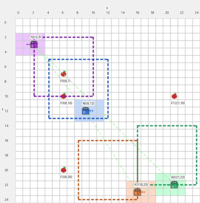
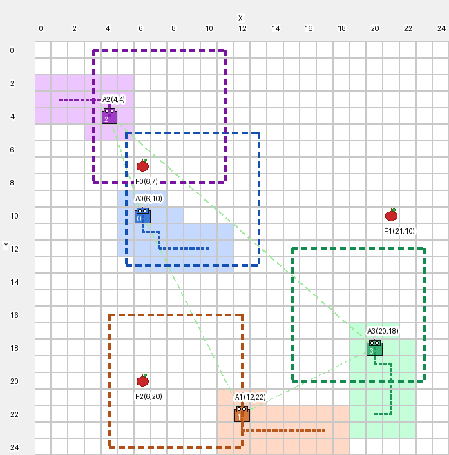
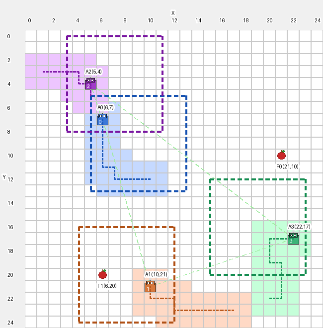
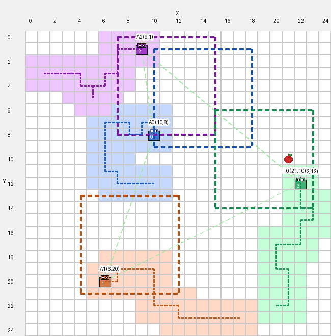
Figure 4 shows the execution trajectory of a trained AHPG model over a complete episode. The strategic layer learns to assign non-overlapping regions that collectively tile the grid, initially placing agents in corners and then adapting assignments to unexplored areas. Agents balance region compliance with opportunistic resource collection. By frame (e), full resource collection with maintained spatial coordination validates the effectiveness of bidirectional hierarchical control.

VII CONCLUSION

This paper introduced CHMAS, a hierarchical MARL framework based on bidirectional coupling between strategic and tactical layers. By enabling strategic planning with exclusive global state access while maintaining distributed tactical execution, CHMAS provides a new architectural paradigm for coordinating agents across multiple temporal scales. The asynchronous update protocol, with a decaying strategic step size schedule, manages the non-stationarity inherent in hierarchical learning and admits $\mathcal{O}(\log K/\sqrt{K})$ convergence guarantees for the strategic layer.

The bidirectional coupling mechanism offers a principled approach to constrained reinforcement learning: strategic guidance encodes global constraints while tactical feedback ensures feasibility, with $\lambda$ providing tunable constraint satisfaction.

References

[1] A. Agarwal, S. M. Kakade, J. D. Lee, and G. Mahajan (2020) Optimality and approximation with policy gradient methods in markov decision processes. In Conference on learning theory, pp. 64–66. Cited by: Remark 3.
[2] P. Bacon, J. Harb, and D. Precup (2017) The option-critic architecture. In Proceedings of the AAAI Conference on Artificial Intelligence, Vol. 31. Cited by: §I.
[3] V. S. Borkar (1997) Stochastic approximation with two time scales. Systems & Control Letters 29 (5), pp. 291–294. Cited by: §III-B.
[4] B. Colson, P. Marcotte, and G. Savard (2007) An overview of bilevel optimization. Annals of Operations Research 153 (1), pp. 235–256. Cited by: §III-A.
[5] P. Hernandez-Leal, B. Kartal, and M. E. Taylor (2019) A survey and critique of multiagent deep reinforcement learning. Autonomous Agents and Multi-Agent Systems 33 (6), pp. 750–797. Cited by: §I, §I.
[6] M. Hong, H. Wai, Z. Wang, and Z. Yang (2023) A two-timescale stochastic algorithm framework for bilevel optimization: complexity analysis and application to actor-critic. SIAM Journal on Optimization 33 (1), pp. 147–180. Cited by: §III-A.
[7] T. D. Kulkarni, K. Narasimhan, A. Saeedi, and J. Tenenbaum (2016) Hierarchical deep reinforcement learning: integrating temporal abstraction and intrinsic motivation. In Advances in Neural Information Processing Systems, Vol. 29. Cited by: §I.
[8] R. Lowe, Y. I. Wu, A. Tamar, J. Harb, P. Abbeel, and I. Mordatch (2017) Multi-agent actor-critic for mixed cooperative-competitive environments. In Advances in Neural Information Processing Systems, Vol. 30. Cited by: §I.
[9] O. Nachum, S. S. Gu, H. Lee, and S. Levine (2018) Data-efficient hierarchical reinforcement learning. Advances in Neural Information Processing Systems 31. Cited by: §I.
[10] A. Nedic, A. Ozdaglar, and P. A. Parrilo (2010) Constrained consensus and optimization in multi-agent networks. IEEE Transactions on Automatic Control 55 (4), pp. 922–938. Cited by: §II-A.
[11] Y. Nesterov (2012) Efficiency of coordinate descent methods on huge-scale optimization problems. SIAM Journal on Optimization 22 (2), pp. 341–362. Cited by: §III-B.
[12] T. T. Nguyen, N. D. Nguyen, and S. Nahavandi (2020) Deep reinforcement learning for multiagent systems: a review of challenges, solutions, and applications. IEEE transactions on cybernetics 50 (9), pp. 3826–3839. Cited by: §I.
[13] R. Olfati-Saber, J. A. Fax, and R. M. Murray (2007) Consensus and cooperation in networked multi-agent systems. Proceedings of the IEEE 95 (1), pp. 215–233. Cited by: §II-A.
[14] S. Pateria, B. Subagdja, A. Tan, and C. Quek (2021) Hierarchical reinforcement learning: a comprehensive survey. ACM Computing Surveys 54 (5), pp. 1–35. Cited by: §I, §II-D.
[15] G. Qu, Y. Lin, A. Wierman, and N. Li (2020) Scalable multi-agent reinforcement learning for networked systems with average reward. Advances in Neural Information Processing Systems 33, pp. 2074–2086. Cited by: §I.
[16] T. Rashid, M. Samvelyan, C. S. De Witt, G. Farquhar, J. Foerster, and S. Whiteson (2020) Monotonic value function factorisation for deep multi-agent reinforcement learning. Journal of Machine Learning Research 21 (178), pp. 1–51. Cited by: §I.
[17] J. Schulman, F. Wolski, P. Dhariwal, A. Radford, and O. Klimov (2017) Proximal policy optimization algorithms. arXiv preprint arXiv:1707.06347. Cited by: §IV-B.
[18] A. Sinha, P. Malo, and K. Deb (2018) A review on bilevel optimization: from classical to evolutionary approaches and applications. IEEE Transactions on Evolutionary Computation 22 (2), pp. 276–295. Cited by: §III-A.
[19] R. S. Sutton, D. Precup, and S. Singh (1999) Between MDPs and semi-MDPs: a framework for temporal abstraction in reinforcement learning. Artificial Intelligence 112 (1-2), pp. 181–211. Cited by: §I.
[20] N. Tishby, F. C. Pereira, and W. Bialek (2000) The information bottleneck method. arXiv preprint physics/0004057. Cited by: §II-D.
[21] A. S. Vezhnevets, S. Osindero, T. Schaul, N. Heess, M. Jaderberg, D. Silver, and K. Kavukcuoglu (2017) Feudal networks for hierarchical reinforcement learning. In International Conference on Machine Learning, pp. 3540–3549. Cited by: §I.
[22] M. A. Wiering et al. (2000) Multi-agent reinforcement learning for traffic light control. In Machine Learning: Proceedings of the Seventeenth International Conference (ICML’2000), pp. 1151–1158. Cited by: §I.
[23] K. Zhang, Z. Yang, and T. Başar (2021) Multi-agent reinforcement learning: a selective overview of theories and algorithms. Handbook of Reinforcement Learning and Control, pp. 321–384. Cited by: §I, Definition 2, Remark 1.
[24] K. Zhang, Z. Yang, H. Liu, T. Zhang, and T. Basar (2018) Fully decentralized multi-agent reinforcement learning with networked agents. In International Conference on Machine Learning, pp. 5872–5881. Cited by: §I.