[1]Martin Alexander Memmesheimer [1]Claudia Redenbach 1]Department of Mathematics, RPTU University Kaiserslautern-Landau, 67663 Kaiserslautern, Germany email: martin.memmesheimer@rptu.de, claudia.redenbach@rptu.de
Fitting the topology of synthetic particle systems with a novel graph representation
Abstract
The shape and arrangement of particles in a material determine its macroscopic properties. The generation of synthetic data with varying particle structure, often represented as 3D voxel images, combined with simulation of macroscopic properties reveals structure-property relations. Most particle generation models focus on single-particle characteristics like shape and size. We aim at fitting the topology of the particle system using tools from persistent homology. However, the large size of the required 3D image data makes existing methods computationally infeasible. We bridge this gap by introducing a novel graph representation of particle systems and transferring the computation of persistent homology from the image domain to the graph domain. This yields a postprocessing method for synthetic images of particle systems, that is independent of the underlying generation method and improves topological and geometrical agreement with real particle systems while preserving morphological characteristics such as the particle size distribution.
Introduction
Particle systems occur in a wide range of natural and engineered materials, including sand, gravel, microdiorite, concrete, iron ore or pigments in coatings. Their mechanical behavior has been the subject of extensive research [1]. Both the geometry of individual particles [2, 3, 4] and the topology and connectivity of the particle system [5, 6, 7] have been shown to strongly influence its macroscopic behavior. In other applications, such as active protective coatings, leaching of pigment particles is the determining process [8]. Also in this case, the connectivity of the particle system is decisive for the coating performance.
X-ray micro-computed tomography (CT) provides the capability to capture the complex three-dimensional geometry of particle systems. However, the acquisition of CT images requires specialized and costly equipment. As a result, only limited amounts of data are available. Thus, the use of data-driven approaches for the analysis of microstructure-property relationships in particulate materials is limited.
The generation of synthetic data is a promising way to circumvent the issues posed by a lack of data. A key component of the generation pipeline is the placement of particles, for which various strategies have been proposed, including random sequential adsorption [9], matching morphological descriptors [10], random tessellations [11], and rigid body simulations [12], which aim to reproduce various statistical and physical characteristics of particle systems. Many downstream applications require an accurate reproduction of the topological structure, including connectivity and higher-dimensional topological features, which existing generation methods typically do not explicitly optimize.
In recent years, there has been a growing interest in integrating topological data analysis, and in particular persistent homology, into synthetic data generation pipelines [13, 14, 15]. Persistent homology is a powerful tool that captures the topological characteristics of data through a summary statistic known as the persistence diagram. By incorporating persistence homology based loss terms, topological optimization has also been applied to a variety of tasks outside of synthetic data generation, including surface matching [16], point cloud processing [17], and topological simplification [18]. While many existing approaches are tailored to specific applications, Carriere et al. [19] introduced a general framework for topological optimization. However, the direct application of existing methods to three-dimensional CT images of a particle system is computationally prohibitive due to their large size. Furthermore, particle-specific information of the CT image cannot be exploited when computing persistent homology in the image domain.
To address these issues, we propose a novel graph representation of particle systems, which enables topological optimization as a postprocessing step for synthetic images, independent of the underlying generation method. Our approach consists of three stages. First, we compute the graph representation on both a real and synthetic image. Next, we apply topological optimization in the graph domain to align the topology of the synthetic graph with that of the real graph. Finally, we return to the image domain by reconstructing an image from the particle graph, whose structure enables an accurate recovery of both particle shapes and the topology of the particle system. Our proposed graph representation offers several advantages for the topological optimization. It leverages particle-specific information while simultaneously reducing the computational cost. Furthermore, it provides a natural interpretation of the optimization in the image domain. In particular, each gradient update in the graph domain can be interpreted as a local deformation of the particle boundary in the image domain.
Results
Graph Representation of Particle Systems
Applying the topological optimization framework directly to persistence diagrams computed from the image representation of the particle system has several drawbacks, including high computational cost and the need to binarize the image, which converts explicit particle information into implicit information. In the following, we introduce a novel graph representation of particle systems that mitigates the issues posed by the image representation.
The idea of the graph representation is as follows. Each particle in the image is represented as a node in the graph. An edge between two nodes is introduced if the particles are connected by an unobstructed line segment that does not intersect another particle. Since the goal of this work is the generation of topology-aware synthetic data, it is important that we can transition back to the image domain in a topology-preserving manner. To achieve this, we enrich the graph with additional geometric information on its edges. In particular, we associate with each edge a start and end point of a shortest unobstructed line segment. The image is then reconstructed by computing the convex hull of all edge features associated with a given particle. We now formalize this construction.
A labeled three-dimensional image is formally represented by a function , where is the image domain and is a set of labels. The elements are called pixels or voxels. A partition of the image domain is given by the sets for . is called the background set and the union of the individual particles is called the foreground set.
Definition.
Given a particle system, represented by a labeled image . For each pair of foreground labels with , we define the set of admissible point pairs
| (1) |
where is the set of voxels on the line segment between and . The particle graph is then defined by
-
•
.
-
•
.
-
•
.
-
•
with
(2)
A few remarks on the graph representation: there is a one-to-one correspondence between nodes and particles, and we will use the terms interchangeably in the following. The node features store the centers of mass of the corresponding particles. While this information is not strictly required for the downstream algorithm, it can improve the stability of the reconstruction near the boundaries.
The edge features store the end points of the line segment associated with an edge. These are essential for the reconstruction, as they encode the geometric relationship between two particles. In general, the minimizing argument in Eq. (2) is not unique. To ensure that is well defined, we select an arbitrary pair at which the minimum is attained. The condition is included in since it imposes a canonical ordering on the undirected edge .
In practice, we compute the particle graph by selecting the first pair encountered that attains the minimum in Eq. (2). To compute such a pair efficiently, it suffices to consider only pairs of boundary voxels of the respective particles. Admissibility of each such pair is determined using Bresenham’s line algorithm [20].
While the full graph contains the most information, the topologically relevant information is expected to be captured primarily by short edges, as features in persistence diagrams are generally associated with spatially localized structures. This motivates using a thresholded version of the graph. For a given threshold , the thresholded graph is obtained by restricting the edge set to
| (3) |
and to . Computing from an image is significantly faster than computing the full graph . For simplicity, we denote the thresholded graph by for the remainder of the paper.
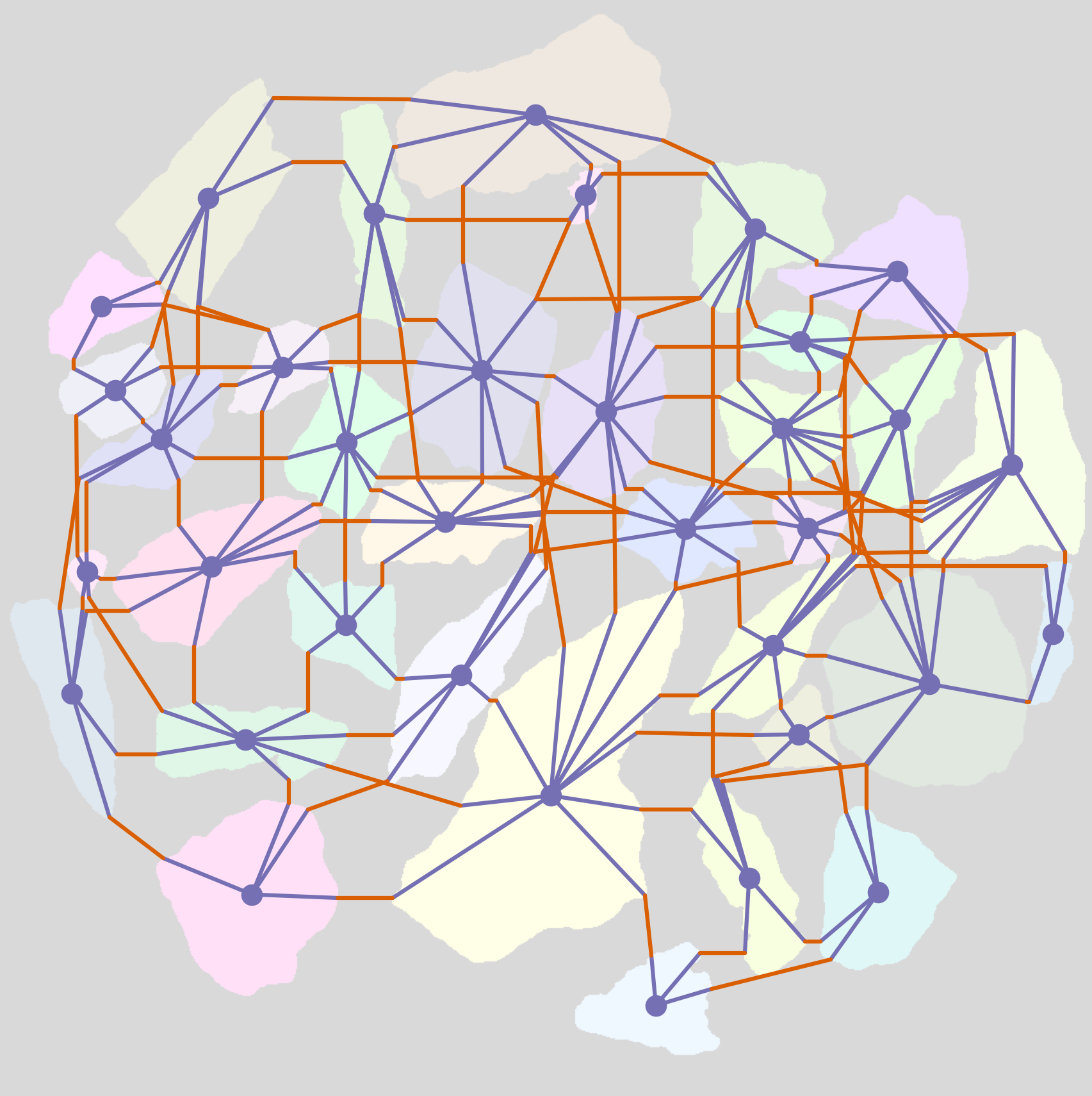

In Figure 1, we visualize the idea of the graph representation in 2D on a slice taken from a computed tomography scan of recycled concrete particles. The role of the node and edge features is clearly visible. In particular, connecting the edge features associated with a single particle and filling the interior of the resulting polygon approximately recovers the particle’s shape and size, except for particles at the sample boundary. In the following, we extend this reconstruction to three-dimensional images.
Given a three-dimensional image and its (thresholded) particle graph , we now define the reconstructed image . We aggregate all points associated with a vertex in a set . More precisely, contains the center of mass as well as, for all edges containing , the point in which belongs to . The reconstructed particle is then defined as the convex hull of , i.e. . If two reconstructed particles overlap, the voxels in their intersection are assigned to the particle with the larger label. The reconstructed image is then given by
| (4) |
The reconstruction can be followed by several postprocessing steps. Usually, we apply a morphological closing [21] with a ball of radius to close one voxel wide gaps between particles that result from the discretization of the reconstructed convex hull onto the voxel grid.
Moreover, the reconstruction via convex hulls yields very regular and smooth particle boundaries, which differ noticeably from the boundaries in the real images. To recover more realistic boundary irregularities, we can add simplex noise [22, 23] to the particle boundary as a final postprocessing step.
Simplex noise generates a spatially continuous noise function, typically in the interval . By scaling the coordinates of the boundary with a frequency parameter before evaluating the noise function and multiplying the resulting noise by a magnitude parameter , both the frequency and amplitude of the boundary perturbations can be controlled. More precisely, given a boundary point and a simplex noise function , we perturb the boundary according to
| (5) |
where denotes the outward unit normal vector at x. Smaller values of and produce smoother boundaries, whereas larger values result in more irregular boundaries. The ability to control both the frequency and amplitude of the perturbations makes simplex noise well suited to our application.
Comparison of Real and Reconstructed Images


Figure 2 shows a side-by-side comparison of the real and reconstructed image, as well as a comparison of an individual particle and its corresponding reconstructed particle with and without simplex noise. Both particle shape and spatial arrangement are accurately recovered in the reconstruction. Compared with the previous 2D example, boundary artifacts are considerably less pronounced in the 3D reconstruction. Furthermore, the addition of simplex noise improves the visual appearance of the particle boundary. To quantitatively assess the reconstruction, we require a measure for evaluating its topological similarity, which is introduced in the next section.
Persistent Homology
In this section, we introduce persistent homology and describe its application to both the image and the graph representation of particle systems. Its foundation was laid in the works of Edelsbrunner et al. [24] and Zomorodian and Carlson [25] with applications to point clouds. Since then, it has been applied to various types of data, including images and graphs.
Topology studies properties that are invariant under continuous deformations. For example, a circle and an ellipse are topologically equivalent. The topological features of interest for this work are connected components (D), loops (D, e.g. the tunnel in a torus), and cavities (D, e.g. the interior of a sphere). The general idea of persistent homology is to associate data with a topological space and study how its topological features change along a filtration, i.e., a nested sequence of topological subspaces ending in the full space.
To efficiently compute persistent homology, it is important to have combinatorial instead of geometrical descriptors of the topological spaces. For graphs, one typically uses simplicial homology. It can also be used for image data after triangulating the image domain, e.g., using a Freudenthal triangulation [26]. Here, we use cubical homology, which operates directly on the voxel grid and therefore provides a natural framework for image data. We introduce only the basic ideas and omit many technical details. For a comprehensive introduction to simplicial persistent homology, we refer the reader to Edelsbruner and Harer [27], and for cubical homology to Kaczynski et al. [28].
Simplicial homology is based on (abstract) simplicial complexes. An (abstract) simplicial complex on a vertex set is a family of subsets of that satisfies the following properties:
-
1.
For every , is in .
-
2.
For every , every subset of is also contained in .
The elements of are called simplices. The dimension of a simplex is given by , and the dimension of is the maximum dimension of its simplices.
Simplicial complexes generalize (undirected) graphs with node set and edge set . By identifying a vertex with the singleton , a graph can be viewed as a one-dimensional simplicial complex . Although it is possible to study the topology of a graph as a one-dimensional simplicial complex, it is usually more informative to construct a higher-dimensional simplicial complex from it.
A widely used construction is the Vietoris-Rips (VR) complex. Given a set of points , a parameter , and symmetric distance function , it is defined by
| (6) |
For a graph , whose edges are equipped with a positive weight function , a distance function can be defined by
| (7) |
The corresponding VR complex is then denoted by . Varying induces a filtration .
The application of persistent homology via cubical homology is based on an embedding of the discrete image domain into . Each voxel is associated with the cube
| (8) |
The union of all such cubes is a subset of , which inherits the subspace topology. A filtration is then obtained from the sublevel sets of a function . Each sublevel set is associated with a topological space given by the union of the embedded voxels whose function values do not exceed .
For grayscale images , sublevel sets can be computed directly on . For binary images, this yields limited information, since the sublevel sets change only at two threshold values. Therefore, is usually obtained by a distance transform
| (9) |
which assigns every pixel its distance to the nearest foreground pixel. Labeled images are first binarized by setting all pixels with to before computing the distance transform.
The classical summary statistic of a persistent homology computation is a collection of persistence diagrams, one for each dimension of topological features. For each dimension , the persistence diagram consists of points , which lie above the diagonal in . Each point represents an -dimensional topological feature that appears in the filtration at birth time and disappears at death time . Formally, a persistence diagram is a finite multiset of points supported on . In addition, the diagonal is included with infinite multiplicity. This is required to ensure the existence of a matching between two diagrams, which classical metrics rely on.
We note that some topological features may persist throughout the filtration and never disappear. Such features have infinite death time and are referred to as essential features. In particular, at least one feature in the -dimensional topology is essential, since at least one connected component must persist through the filtration. In higher dimensions, essential features may occur depending on the data. In our application, they never occur in persistence diagrams computed from images and very rarely occur in diagrams computed from graphs. Since essential points are difficult to handle within the optimization framework, we discard them from the persistence diagrams. As their proportion in our data is well below one percent, the information loss due to their omission is negligible. In the subsequent analysis, we always assume that no essential points exist.
To define a loss function for the optimization framework, we require a distance measure between the persistence diagram of the synthetic and real data. A classical metric is the -Wasserstein distance. Let be two persistence diagrams with finitely many off-diagonal points, as is always the case for our data. The -Wasserstein distance is defined as
| (10) |
where the infimum is taken over all possible bijections . We slightly abuse notation in the above definition by denoting the perpendicular distance of to the diagonal by , and by setting . The inclusion of the diagonal in the persistence diagrams ensures that a bijection exists. Consequently, the feasible set of bijections is nonempty. Since all costs are nonnegative, the objective function in the minimization problem is bounded from below by such that the Wasserstein distance is well-defined and finite.
Validation of the Reconstruction Algorithm
For method validation, we check that topological and geometric characteristics of the reconstructed particles reproduce the characteristics observed in the data.
CT Images of Recycled Concrete


We test the reconstruction quality on the four images of recycled concrete (RC) shown in Figure 3. Details on the materials and the imaging are given in the methods section. For every image we compute the thresholded particle graph with threshold . From that graph we compute the reconstructed image following Eq. (4) and postprocess it with a morphological closing of radius .
We report five metrics in total, two pixelwise and three topological metrics. For measuring the pixelwise accuracy, we report the Dice score [29] which, for two sets and is given by
| (11) |
We report the mean of the Dice scores of the individual particles in the labeled image, and the Dice score of the full image which takes the entire foreground as the ground-truth set. For the topological metrics we compute the persistence diagrams of the real and reconstructed images as described earlier. For the - and -dimensional persistence diagrams we remove noisy features with a persistence of or less from the persistence diagram, i.e. points with . Then we compute the -Wasserstein distances. As the Wasserstein distance is not an absolute measure, we report normalized Wasserstein distances for the - and -dimensional diagrams obtained by dividing each distance by the -Wasserstein distance between the persistence diagram of the real image and the empty diagram (containing only the diagonal). This allows the interpretation of the value as the fraction of total topological change during the reconstruction. For the -dimensional diagrams we neither do the filtering nor the normalization. Since all binarized real images in our dataset consist of a single connected component, their -dimensional persistence diagrams are empty and the normalization is therefore not well defined. The resulting metrics are denoted by with denoting the dimensionality of the persistence diagrams.
Reconstruction Quality
| Image | Mean Dice | Dice | |||
|---|---|---|---|---|---|
| RC | |||||
| RC | |||||
| RC | |||||
| RC |
The results are reported in Table 1. The observed Dice scores are around , indicating a high degree of overlap between the particles in the reconstructed and the real image. Moreover, the mean Dice score suggests that this performance is not driven by a few large particles dominating the metric, but rather by a consistent overlap across individual reconstructed particles. We also observe a very strong performance across the topological metrics. The -dimensional topology shows that the reconstructed image again contains a single connected component. In the -dimensional topology approximately of the total topology is preserved through the reconstruction, while the corresponding value for the -dimensional topology is approximately .
The reported values correspond to the reconstruction without the addition of simplex noise. We also tested the effect of incorporating simplex noise and observed that the Dice scores consistently decreased by approximately . The topological metrics varied only slightly, being consistent in , improving for and deteriorating for . Overall, simplex noise does not have a consistent positive or negative effect on the reconstruction quality. Therefore, it is omitted from subsequent evaluations.
The observations in this section are robust w.r.t. the threshold value . We evaluated the reconstructions for thresholds between and . When increasing the threshold, the Dice scores improved from to , while the topological metrics showed no clear trend but varied only slightly for both the - and -dimensional topology. In the following, is used as it most accurately reproduces the volume fraction of the particle systems.
Topological Loss Term and Differentiability
The idea of our generative framework is as follows. First, we generate an initial synthetic particle system, then we match the topology of the corresponding particle graph with the topology of the particle graph of the real data. Finally, we reconstruct an image from the optimized synthetic graph. In this section, we focus on the topological optimization by defining a suitable loss term that can be minimized using gradient-based optimization.
Assume that we are given a thresholded particle graph , computed from a synthetic image of a particle system with an arbitrary initial generation method. The optimization objective is to match the topology of with the persistence diagrams of a particle graph computed from a real image of a particle system. The logical candidate for the loss function in the topological optimization is the -Wasserstein distance. In order to compute it, we first need to compute the persistence diagram for a given homology dimension of . As introduced in the persistent homology section, the persistence diagrams of graphs with a weight function on the edges can be computed with the VR-complex. In the case of the particle graph, we define such a weight function by
| (12) |
where . We denote the resulting persistence diagram of the -dimensional homology by .
Given a set of dimensions , we want to optimize over persistence diagrams and target diagrams . The logical candidate for the loss term of the optimization problem is
| (13) |
Using instead of is preferable as it avoids dealing with the square root in the gradients. This loss is not yet differentiable, since the -Wasserstein contains an infimum in its definition. However, the -Wasserstein distance can be rewritten in a differentiable form as
| (14) |
where is an optimal matching at which the infimum is attained. It is clear that such an optimal matching always exists, since there are only finitely many different matchings between the finite off-diagonal parts of the diagrams.
As discussed by Carriere et al. [30], the optimal matching is in general unique and therefore the -Wasserstein distance is differentiable almost everywhere. However, the matching is an unstable quantity in the sense that slight perturbations in either or may lead to a significantly different optimal matching which consequently results in large changes in the corresponding gradients. This may cause instability in a gradient-based optimization framework. Instead of using the -Wasserstein distance directly in the optimization, they propose to add an entropic regularization term based on the optimal transport problem, which improves the stability of the gradients. For a given regularization parameter , we denote the entropic regularized -Wasserstein distance by . Details on the optimal transport theory and the entropic regularization term are provided in the Methods section.
Since provides stable gradients, it is a well suited option for the loss term in a gradient descent scheme. In particular, for a regularization parameter , we replace the Wasserstein distances in Eq. (13) by their regularized approximations. The regularized loss term is given by
| (15) |
To ensure end-to-end differentiability, the persistence diagrams must be differentiable w.r.t. the edge features. Since they are computed from a Vietoris-Rips filtration, each birth and death value corresponds to a value of the distance function from Eq. (7). Since the values of the distance function are either independent of the edge features or depend on the function from Eq. (12), it suffices to verify that is differentiable. While the -norm is not differentiable when one of its components is , a subgradient can be obtained by setting the corresponding component to . Since subgradients can be employed in gradient-based optimization methods, this ensures applicability of our loss function.
Advantages of the Graph Representation
Computing a graph and reconstructing an image introduces a domain gap that can both reduce or improve the quality of the synthetic images. Therefore, it is not obvious why the proposed graph representation should be preferred over operating directly on the image representation. In the following, we discuss the drawbacks of the image representation and the advantages of the proposed graph-based formulation within the optimization framework.
To apply persistent homology to a labeled image and compute its persistence diagrams, a binarization is required. With this step, particle specific information is represented implicitly rather than explicitly. Moreover, even a binary image is not well suited for a gradient descent algorithm, as it is unclear how to define meaningful gradient updates. The standard approach to mitigate this issue is by relaxing the image to continuous values between and , which in turn requires thresholding to recover a binary representation for the computation of the persistence diagrams.
One of the key advantages of synthetic data over real data is, that a perfect segmentation is known. However, the implicit representation of particle specific information removes this advantage since the data is no longer explicitly labeled and segmentation must be performed after the optimization. Moreover, the implicit representation allows particles to merge or the creation of new particles during the optimization. While this may still yield the desired topological properties, it can drastically alter other characteristics, such as the particle size distribution.
Another drawback of operating on the image domain is the high computational cost. Three-dimensional CT images typically contain a large number of voxels (e.g., the images of recycled concrete considered in this work have a size of approximately voxels). Computing a persistence diagram on such an image is computationally very expensive. Even after downsampling, the computational cost remains high. This makes a gradient descent algorithm infeasible in practice, as it requires iterative computation of persistence diagrams.
The graph representation mitigates all of these issues. Since the edge features are continuous, gradient-based optimization can be applied directly with huge computational benefits. Furthermore, the graph preserves the explicit particle information, and the reconstructed image is inherently segmented. The explicit particle information also allows the gradient updates to be interpreted as a local deformation of the particle boundary in the neighbourhood of the moved edge features. In particular, particles cannot merge, and no new particles can be created during the optimization algorithm.
A naturally arising question is why we propose a graph-based representation rather than using a marked point cloud. The reconstructed image does indeed only depend on the points stored in the edge features and is independent of the actual edge set (cf. Eq. (4)). By setting the distance of two points with the same mark to and applying the VR filtration to the point cloud, this would provide a reasonable representation of the topology of the particle system.
However, this approach is computationally infeasible in practice. The cost of computing persistence diagrams via the Vietoris-Rips filtration depends on the number of simplices in the filtration, which grows rapidly with the number of input points. In our setting, the particle graphs contain between and edges, corresponding to a point cloud of to points. Even when using a threshold on the filtration values of the simplices, the computational cost is prohibitively large.
Rather than representing each point separately, our proposed graph representation aggregates all points belonging to the same particle into a single graph node and encodes their geometry in the weight function . As a result, a configuration of over points is encoded as a graph with to nodes. This substantially reduces the size of the induced VR complexes in the filtration and, in turn, the computational cost of persistent homology.
Synthetic Images of Concrete
In this section, we evaluate our method on synthetic images of recycled concrete. For each of the four real concrete images shown in Figure 3, we generated synthetic images with the random sequential adsorption algorithm (RSA). Details on their generation with RSA are given in the methods section. Then, we optimized the topology of the corresponding thresholded particle graphs with using the regularized loss term from Eq. (15) for different and the Adam optimizer [31]. Finally, we reconstructed images from the graphs. Before evaluation we applied a morphological closing of radius to both the RSA and the reconstructed images and refrained from adding simplex noise to the reconstruction. We compare the optimized reconstructed images to the real and the RSA images in terms of the number of particles, the volume fraction, the Wasserstein distances, the particle volume and surface area distribution, and the geometric tortuosity.
Number of Particles
| Image Type | RC | RC | RC | RC |
|---|---|---|---|---|
| Real Image | 510 | 517 | 579 | 504 |
| RSA | 510 | 513.438 | 575.125 | 503.875 |
Volume Fraction
| Image Type | RC | RC | RC | RC |
|---|---|---|---|---|
| Real Image | 0.410 | 0.454 | 0.472 | 0.421 |
| RSA | 0.410 | 0.455 | 0.472 | 0.422 |
| Reconstruction | 0.402 | 0.446 | 0.469 | 0.415 |
| 0.405 | 0.448 | 0.471 | 0.417 | |
| 0.415 | 0.458 | 0.482 | 0.428 | |
| 0.406 | 0.452 | 0.476 | 0.422 | |
| 0.416 | 0.458 | 0.482 | 0.429 | |
| 0.409 | 0.454 | 0.478 | 0.425 | |
| 0.418 | 0.462 | 0.487 | 0.434 | |
| 0.418 | 0.462 | 0.487 | 0.434 |
Since the particle systems in the real images are relatively dense, it is not guaranteed that the RSA algorithm is able to place all particles. Table 2 reports the number of particles in the real images together with the average number of particles placed in the corresponding RSA images. We observe that all particles could be placed in RC, while in RC only particles across all synthetic images could not be placed. For RC and RC, on average around to particles per image are missing. Nevertheless, the volume fractions of the real and RSA images are nearly identical, see Table 3. In fact, the volume fraction of the RSA images is sometimes even slightly larger than that of the real images which is caused by the morphological closing applied to the RSA images. Furthermore, we observe that the reconstruction using the unoptimized graph leads to a slight loss of volume fraction. Optimizing the graph increases the volume fraction of the corresponding reconstructed images, with most of this increase coming from the -dimensional topology.
-Wasserstein Distances
| Image Type | ||||||
|---|---|---|---|---|---|---|
| RC | RC | |||||
| RSA | ||||||
| Reconstruction | ||||||
| RC | RC | |||||
| RSA | ||||||
| Reconstruction | ||||||
The main objective of the optimization is to decrease the topological difference between the real and synthetic images. We report the same topological metrics , computed from the -Wasserstein distances, as defined in the ”Validation of the Reconstruction Algorithm” section. The results are shown in Table 4. We observe that the domain gap introduced by computing the reconstructed image without any optimization can have both a positive or negative effect on the topology. In particular, we observe a positive effect across all four images in and and a negative effect in . However, the differences are relatively small such that the reconstructions of the optimized graphs outperform the RSA images consistently in all three dimensions.
A first observation is that optimizing w.r.t. a given dimension consistently improves the corresponding metric in the resulting image. In particular, the best observed values for each dimension are always achieved by an optimization that uses the same dimension. Furthermore, we observe that incorporating additional dimensions usually helps, e.g. the best observed values of and are always attained when both of them are in . However, is usually worse if additional dimensions are included during the optimization.
We now consider the best observed values for individually and compare them with the values of the synthetic RSA images and unoptimized reconstructions. For a perfect agreement is achieved for RC and RC across all synthetic images, while the errors are reduced by over for RC and RC. For , the optimized images improve by between and relative to the unoptimized reconstructions and by between and relative to the RSA images. For , the improvement relative to the unoptimized reconstructions ranges from approximately for RC to between and for the other three images. Compared with the RSA images, the improvements increase to approximately for RC and about for the other three images. Overall, these results demonstrate that optimization on the graph representation consistently improves the image topology across all three dimensions.


The RSA algorithm just places the original particles at new positions, such that the resulting images preserve the particle volume and surface area distributions exactly. To assess the fit after topological optimization and reconstruction, we computed histograms for the particle volume and particle surface area distributions of the real image, as well as the mean distributions of the RSA images, their reconstructions and the images optimized with . To improve visibility, we excluded the largest of particles across the four images. The resulting histograms are shown in Figure 4 and Figure 5.
As expected, the particle volume and surface area distributions of the real and RSA images (blue) are nearly identical. The reconstructed and optimized images (green) also have distributions that are overall similar to the real distribution. Nevertheless, several differences can be observed across all four images. In the particle volume distribution, the volume of smaller particles tends to decrease further during reconstruction, whereas the frequencies of the largest particles increase. A likely explanation is that large particles might have large concave areas, which are filled by the convex hull during reconstructions. The particle surface area is shifted slightly towards smaller values. This is expected, since the convex hull produces locally flat boundaries, whereas the boundaries in the real images are more irregular. Overall, the reconstruction introduces only minor changes to both distributions while preserving their characteristics.
Geometric Tortuosity
| Image Type | RC | RC | RC | RC |
|---|---|---|---|---|
| Real Image | ||||
| RSA | ||||
| Reconstruction | ||||
Finally, we study the geometric tortuosity of the real and the synthetic images. The geometric tortuosity is based on the geodesic distance between two foreground pixels, i.e., the length of the shortest path connecting two pixels while not leaving the foreground. The geometric tortuosity between the two pixels is then defined as the ratio of their geodesic distance and their Euclidean distance. For more details see Soille [32]. To compute the geometric tortuosity of an image in a certain direction, one usually computes all geometric distances of border foreground pixels to the opposite image border and then averages the corresponding tortuosities.
We report the geometric tortuosity in the height direction of the scanning container. To avoid boundary effects, we computed the geodesic distances between the image slices and . The results are shown in Table 5. We observe a positive domain gap from the RSA images to their reconstructions. This can be explained by two reasons. First, as indicated by the lower values in Table 4, the reconstructed images exhibit a higher connectivity than the RSA images. Consequently, they contain more possible paths, which reduces the geometric tortuosity. Second, the reconstructed convex particles allow for shorter paths than the original particles that may contain concavities. Since all the synthetic images exhibit a higher geometric tortuosity than the corresponding real images, both effects move the tortuosity in the desired direction. Furthermore, we observe that the optimization decreases the tortuosity further. Relative to the tortuosities of the reconstructed images, the best observed tortuosities reduce the deviation from the tortuosity of their respective real image by to for three of the four images and by for RC. Comparing the tortuosities for different optimization sets reveals that the improvement is mainly driven by the optimization of the -dimensional topology, while the best performance is achieved when optimizing over all three dimensions.
These results show that applying our optimization to synthetic particle systems yields consistent improvements in topological and geometric metrics, while only slightly affecting the particle geometry.
Discussion
This paper proposed an optimization scheme that can be applied to arbitrarily generated synthetic particle systems to improve topological and physical characteristics. To this end, we introduced a novel graph representation of the particle system, which leverages explicit particle information and offers computational advantages.
Our validation shows that our method consistently improves the topological quality and the geometric tortuosity of the generated images while preserving other important characteristics of the particle systems, including the number of particles and the distributions of particle volume and surface area.
A first direction for future work is computational efficiency of the method. While our proposed graph representation provides huge computational benefits, the runtime scales with the number of particles and the dimension up to which we compute persistence diagrams. Iteratively computing persistent homology up to dimension on graphs with more than nodes becomes computationally prohibitive. A promising direction for reducing this cost is the use of fast persistence updates based on computations obtained from previous iterations. Such approaches have been explored in various settings [33, 34] and may also be applicable here.
A second research direction is narrowing the domain gap introduced during the reconstruction through the graph representation. In particular, replacing the convex hull used for the particle reconstruction from a set of points with a method capable of modeling concavities in the particle boundaries might likely improve the fit of the reconstruction. One possible alternative is the use of spherical harmonics conditioned on as boundary conditions [11]. This approach introduces a probabilistic component into the reconstruction, whose influence, similar to the addition of simplex noise, would need to be investigated further. Another possible approach is the use of alpha shapes [35] instead of the convex hull. However, the density of boundary points in is insufficient to reliably reconstruct particle boundaries using alpha shapes. While increasing the number of sampled boundary points per particle is straightforward, doing so does not allow for the same graph representation. The logical representation of the sampled points would be a marked point cloud and, as previously discussed, this would render the topological optimization computationally infeasible. Therefore, we expect that developing a method capable of exploiting a larger number of boundary points in combination with alpha shapes, while maintaining computational efficiency, could further improve the observed results.
Methods
CT Images of Particle Systems
We consider a set of four three-dimensional X-ray micro-computed tomography (CT) images of recycled concrete particles. The particle systems were scanned as packed beds in a cylindrical scanning container. The X-ray projections are reconstructed using VGSTUDIO 3.2 (Volume Graphics) by the Feldkamp-David-Kress algorithm [36]. After several postprocessing steps, the image is converted into a binary image using Otsu’s method [37]. The particles are then segmented using the watershed transform [38]. To remove the separation boundaries introduced by the watershed transform, we subsequently apply a morphological closing with a ball of radius voxel. The resulting particle systems are visualized in Figure 3. Further details on the image data and the processing steps can be found in [39].
Random Sequential Adsorption (RSA)
Our framework can be applied to synthetic data generated by an arbitrary method. In our experiments, we use the random sequential adsorption algorithm [9], which is a standard method to generate systems of nonoverlapping particles. Given a set of particles, the algorithm sequentially inserts them into a bounded container. For each particle, uniformly generated candidate positions are tested iteratively. The candidate position is accepted if the particle does not intersect any previously placed particles. Otherwise a new candidate position is tested. If no admissible position is found after a fixed number of tries, the particle is rotated by permuting its axes and the placement procedure is repeated. If the particle cannot be placed in any rotation it is discarded and the algorithm proceeds to the next particle.
The set of particles can be generated by various models, e.g. as the typical cell of a fitted Gibbs-Laguerre tessellation [40] or as Gaussian random fields on the sphere [41, 11]. In this work, we refrain from modelling the particles and just rearrange the particles from the original data.
Checking different positions for valid particle placements scales with the number of voxels in a particle. Therefore, computational cost can be reduced drastically by reducing the image size. In order to both speed up computation and generate synthetic images with the full resolution, we generate two images, one in the original size and one with a downscaled size, when applying RSA. We generate a set of particles for the downscaled image by downsampling the original image with a majority vote in every downsample block. While applying the RSA algorithm, we test the positions in the downscaled image. If a downscaled particle is placed, we also place the original particle at the corresponding position in the full resolution image.
While we always use the full resolution images in our experiments, maintaining the synthetic image at both resolutions has the additional benefit that the graph representation of the particle system can be computed on the downscaled resolution, followed by an upscaling of its features. This decreases the computational cost of the particle graph significantly.
Optimal Transport and Entropic Regularization
Optimal transport is closely related to Wasserstein distances and can be used to study the space of persistence diagrams, see Divol and Lacombe [42]. It provides tools to compare measures by seeking an optimal transport plan which minimizes the cost of transporting the mass from one measure to another. The connection to persistence diagrams arises by representing a persistence diagram as a finite sum of Dirac measures located at its off-diagonal points. However, standard optimal transport theory assumes the two measures to have equal mass, which is generally not the case for persistence diagrams. An extension of the optimal transport problem to measures of different mass has been discussed by various authors [43, 44, 45]. Lacombe et al. [46] show how the Wasserstein distance between persistence diagrams can be computed using the discrete optimal transport formulation. Then they use an entropically regularized version of this problem, introduced by Cuturi [47], to approximate the Wasserstein distance. This regularized version offers several advantages, as it is faster to compute, differentiable and provides more stable gradients. In the following we introduce the necessary background in optimal transport theory, following the notation in Lacombe et al. [46].
Consider two finite discrete measures and with positive weights and points from the upper half plane for and . The discrete optimal transport problem requires that the measures have equal mass, i.e. . The aim is to compute the minimal transportation cost from to w.r.t. some cost matrix . A transportation plan is a matrix whose rows and columns sum up to and , respectively. The transportation polytope
| (16) |
is the set of all transportation plans and the cost of a plan is given by the Frobenius dot product between and . The discrete optimal transport problem is then given by
| (17) |
Solving this linear program becomes intractable for large . To address this, Cuturi [47] proposed to add an entropic regularizer to the formulation. For and , the regularized problem is given by
| (18) |
This formulation has several desirable properties. In particular, it can be solved significantly faster than the unregularized version using Sinkhorn divergences, it has a unique solution , and the cost of the optimal transport goes to as . Furthermore, it is differentiable and provides stable gradients, which is most important for our use. By expressing the -Wasserstein distance as a discrete optimal transport problem, we can use Eq. (18) in our loss term.
A persistence diagram can be associated with a finite sum of Dirac measures where are the off-diagonal points in the diagram and the are their multiplicities. To maintain the behaviour of the diagonal in this association, a virtual diagonal point is added to the measure. Formally, this is done by a linear operator , which assigns the mass of a measure to . Consider the associated measures of two persistence diagrams and the cost matrix
| (19) |
where is the pairwise distance matrix between points of and , and , are the distances of points in , to the diagonal, respectively, Lacombe et al. [46] show that the -Wasserstein distance can be expressed by
| (20) |
The entropic regularized version of Eq. (20) gives rise to an approximation of the -Wasserstein distance. A bound on the approximation error between and its regularized version is proven in [46].
Experiment Details
As described in the previous section, we compute pairs of a downscaled and full resolution synthetic image. The downscaled image size is obtained by scaling each spatial dimension by a factor of . During particle placement, million random positions were tested for each particle and rotation. The computation is done on the GPU.
The particle graphs were computed on the downscaled images using a threshold of , which corresponds to a threshold in the full resolution. Subsequently we scaled the node and edge features of the computed graphs by a factor of to recover the original spatial resolution.
Optimization Hyperparameters
| Hyperparameter | Value |
|---|---|
| Optimizer | Adam |
| Learning rate | |
| Learning rate scheduler | ExponentialLR |
| Exponential decay factor | |
| Number of epochs | |
| Entropic regularization |
References
- \bibcommenthead
- [1] Radjai, F., Roux, J.-N. & Daouadji, A. Modeling granular materials: Century-long research across scales. Journal of Engineering Mechanics 143, 04017002 (2017). URL https://ascelibrary.org/doi/abs/10.1061/(ASCE)EM.1943-7889.0001196.
- [2] Erdogan, S. et al. Three-dimensional shape analysis of coarse aggregates: New techniques for and preliminary results on several different coarse aggregates and reference rocks. Cement and Concrete Research 36, 1619–1627 (2006). URL https://www.sciencedirect.com/science/article/pii/S0008884606001013.
- [3] Fonseca, J., O’Sullivan, C., Coop, M. & Lee, P. Non-invasive characterization of particle morphology of natural sands. Soils and Foundations 52, 712–722 (2012). URL https://www.sciencedirect.com/science/article/pii/S0038080612000819.
- [4] Garboczi, E. Three-dimensional mathematical analysis of particle shape using x-ray tomography and spherical harmonics: Application to aggregates used in concrete. Cement and Concrete Research 32, 1621–1638 (2002). URL https://www.sciencedirect.com/science/article/pii/S0008884602008360.
- [5] Liu, J., Zhou, W., Ma, G., Yang, S. & Chang, X. Strong contacts, connectivity and fabric anisotropy in granular materials: A 3d perspective. Powder Technology 366, 747–760 (2020). URL https://www.sciencedirect.com/science/article/pii/S0032591020302096.
- [6] Papadopoulos, L., Porter, M. A., Daniels, K. E. & Bassett, D. S. Network analysis of particles and grains. Journal of Complex Networks 6, 485–565 (2018). URL https://doi.org/10.1093/comnet/cny005.
- [7] Walker, D. M. & Tordesillas, A. Topological evolution in dense granular materials: A complex networks perspective. International Journal of Solids and Structures 47, 624–639 (2010). URL https://www.sciencedirect.com/science/article/pii/S0020768309004272.
- [8] Zaninović, J. et al. Leaching in active protective coatings observed in-situ by nano-CT using synchrotron radiation. Corrosion Science 263, 113631 (2026). URL https://www.sciencedirect.com/science/article/pii/S0010938X26000405.
- [9] Chiu, S. N., Stoyan, D., Kendall, W. S. & Mecke, J. Stochastic geometry and its applications (John Wiley & Sons, 2013).
- [10] You, H., Kim, Y. & Yun, G. J. Computationally fast morphological descriptor-based microstructure reconstruction algorithms for particulate composites. Composites Science and Technology 182, 107746 (2019). URL https://www.sciencedirect.com/science/article/pii/S0266353819302076.
- [11] Feinauer, J. et al. Stochastic 3d modeling of the microstructure of lithium-ion battery anodes via gaussian random fields on the sphere. Computational Materials Science 109, 137–146 (2015). URL https://www.sciencedirect.com/science/article/pii/S0927025615003845.
- [12] Wang, B., Kingston, A. M., Lösel, P. D. & Creemers, W. Synthetic particle pack generation for augmentation and testing in geological tomographic segmentation. Tomography of Materials and Structures 9, 100072 (2025). URL https://www.sciencedirect.com/science/article/pii/S2949673X25000257.
- [13] Gupta, S., Samaras, D. & Chen, C. Topodiffusionnet: A topology-aware diffusion model. (eds Yue, Y., Garg, A., Peng, N., Sha, F. & Yu, R.) International Conference on Learning Representations, Vol. 2025, 31699–31713 (2025). URL https://proceedings.iclr.cc/paper_files/paper/2025/file/4e889e581d4a6f2be932c6f65e7792a8-Paper-Conference.pdf.
- [14] Liu, J. et al. Topolidm: Topology-aware lidar diffusion models for interpretable and realistic lidar point cloud generation. (eds Laugier, C. et al.) 2025 IEEE/RSJ International Conference on Intelligent Robots and Systems (IROS), 8180–8186 (IEEE, 2025).
- [15] Wang, F., Liu, H., Samaras, D. & Chen, C. Topogan: A topology-aware generative adversarial network. (eds Vedaldi, A., Bischof, H., Brox, T. & Frahm, J.-M.) Computer Vision – ECCV 2020, 118–136 (Springer International Publishing, Cham, 2020).
- [16] Poulenard, A., Skraba, P. & Ovsjanikov, M. Topological function optimization for continuous shape matching. Computer Graphics Forum 37, 13–25 (2018). URL https://onlinelibrary.wiley.com/doi/abs/10.1111/cgf.13487.
- [17] Brüel-Gabrielsson, R., Ganapathi-Subramanian, V., Skraba, P. & Guibas, L. J. Topology-aware surface reconstruction for point clouds. Computer Graphics Forum 39, 197–207 (2020). URL https://onlinelibrary.wiley.com/doi/abs/10.1111/cgf.14079.
- [18] Kissi, M., Pont, M., Levine, J. A. & Tierny, J. A practical solver for scalar data topological simplification. IEEE Transactions on Visualization and Computer Graphics 31, 97–107 (2025).
- [19] Carriere, M. et al. Optimizing persistent homology based functions. (eds Meila, M. & Zhang, T.) Proceedings of the 38th International Conference on Machine Learning, Vol. 139 of Proceedings of Machine Learning Research, 1294–1303 (PMLR, 2021). URL https://proceedings.mlr.press/v139/carriere21a.html.
- [20] Bresenham, J. E. Algorithm for computer control of a digital plotter. IBM Systems Journal 4, 25–30 (1965).
- [21] Ohser, J. & Schladitz, K. 3D Images of Materials Structures (John Wiley & Sons, Ltd, 2009).
- [22] Gustavson, S. Simplex noise demystified (2005).
- [23] Perlin, K. Noise hardware. in real-time shading. SIGGRAPH Course Notes (2001).
- [24] Edelsbrunner, Letscher & Zomorodian. Topological persistence and simplification. Discrete & computational geometry 28, 511–533 (2002).
- [25] Zomorodian, A. & Carlsson, G. Computing persistent homology. Discrete & Computational Geometry 33, 249–274 (2005). URL https://doi.org/10.1007/s00454-004-1146-y.
- [26] Freudenthal, H. Simplizialzerlegungen von beschränkter Flachheit. Annals of Mathematics 43, 580–582 (1942). URL http://www.jstor.org/stable/1968813.
- [27] Edelsbrunner, H. & Harer, J. Computational topology: an introduction (American Mathematical Soc., 2010).
- [28] Kaczynski, T., Mischaikow, K. & Mrozek, M. Cubical Homology, 39–92 (Springer New York, New York, NY, 2004). URL https://doi.org/10.1007/0-387-21597-2_2.
- [29] Mohapatra, R. K. et al. A comprehensive survey to study the utilities of image segmentation methods in clinical routine. Network Modeling Analysis in Health Informatics and Bioinformatics 13, 2 (2023). URL https://doi.org/10.1007/s13721-023-00436-z.
- [30] Carriere, M., Ike, Y., Lacombe, T. & Nishikawa, N. Persistence-based topological optimization: a survey. arXiv preprint arXiv:2603.24613 (2026).
- [31] Kingma, D. P. & Ba, J. Adam: A Method for Stochastic Optimization. (eds Bengio, Y. & LeCun, Y.) 3rd International Conference on Learning Representations, Conference Track Proceedings (2015). URL https://mlanthology.org/iclr/2015/kingma2015iclr-adam/.
- [32] Soille, P. Morphological Image Analysis: Principles and Applications (Springer Berlin Heidelberg, Berlin, Heidelberg, 2004). URL https://doi.org/10.1007/978-3-662-05088-0.
- [33] Cohen-Steiner, D., Edelsbrunner, H. & Morozov, D. Vines and vineyards by updating persistence in linear time. (eds Amenta, N. & Cheong, O.) Proceedings of the Twenty-Second Annual Symposium on Computational Geometry, SCG ’06, 119–126 (Association for Computing Machinery, New York, NY, USA, 2006). URL https://doi.org/10.1145/1137856.1137877.
- [34] Luo, Y. & Nelson, B. J. Accelerating iterated persistent homology computations with warm starts. Computational Geometry 120, 102089 (2024). URL https://www.sciencedirect.com/science/article/pii/S0925772124000117.
- [35] Edelsbrunner, H. & Mücke, E. P. Three-dimensional alpha shapes. ACM Trans. Graph. 13, 43–72 (1994). URL https://doi.org/10.1145/174462.156635.
- [36] Feldkamp, L. A., Davis, L. C. & Kress, J. W. Practical cone-beam algorithm. J. Opt. Soc. Am. A 1, 612–619 (1984). URL https://opg.optica.org/josaa/abstract.cfm?URI=josaa-1-6-612.
- [37] Otsu, N. A threshold selection method from gray-level histograms. IEEE Transactions on Systems, Man, and Cybernetics 9, 62–66 (1979).
- [38] Vincent, L. & Soille, P. Watersheds in digital spaces: an efficient algorithm based on immersion simulations. IEEE Transactions on Pattern Analysis and Machine Intelligence 13, 583–598 (1991).
- [39] Burgmann, S., Godehardt, M., Schladitz, K. & Breit, W. Separation of sand and gravel particles in 3d images using the adaptive h-extrema transform. Powder Technology 404, 117468 (2022). URL https://www.sciencedirect.com/science/article/pii/S003259102200362X.
- [40] Schladitz, K. et al. Geometric modelling of corrosion inhibitor pigments in active protective coatings based on SR-nano-CT images. Progress in Organic Coatings 197, 108762 (2024). URL https://www.sciencedirect.com/science/article/pii/S030094402400554X.
- [41] Furat, O. et al. Artificial generation of representative single li-ion electrode particle architectures from microscopy data. npj Computational Materials 7, 105 (2021). URL https://doi.org/10.1038/s41524-021-00567-9.
- [42] Divol, V. & Lacombe, T. Understanding the topology and the geometry of the space of persistence diagrams via optimal partial transport. Journal of Applied and Computational Topology 5, 1–53 (2021). URL https://doi.org/10.1007/s41468-020-00061-z.
- [43] Chizat, L., Peyré, G., Schmitzer, B. & Vialard, F.-X. Unbalanced optimal transport: Dynamic and kantorovich formulations. Journal of Functional Analysis 274, 3090–3123 (2018). URL https://www.sciencedirect.com/science/article/pii/S0022123618301058.
- [44] Figalli, A. & Gigli, N. A new transportation distance between non-negative measures, with applications to gradients flows with dirichlet boundary conditions. Journal de Mathématiques Pures et Appliquées 94, 107–130 (2010). URL https://www.sciencedirect.com/science/article/pii/S0021782409001627.
- [45] Kondratyev, S., Monsaingeon, L. & Vorotnikov, D. A new optimal transport distance on the space of finite Radon measures. Advances in Differential Equations 21, 1117 – 1164 (2016). URL https://doi.org/10.57262/ade/1476369298.
- [46] Lacombe, T., Cuturi, M. & Oudot, S. Large scale computation of means and clusters for persistence diagrams using optimal transport. (eds Bengio, S. et al.) Advances in Neural Information Processing Systems, Vol. 31 (Curran Associates, Inc., 2018). URL https://proceedings.neurips.cc/paper_files/paper/2018/file/b58f7d184743106a8a66028b7a28937c-Paper.pdf.
- [47] Cuturi, M. Sinkhorn distances: Lightspeed computation of optimal transport. (eds Burges, C., Bottou, L., Welling, M., Ghahramani, Z. & Weinberger, K.) Advances in Neural Information Processing Systems, Vol. 26 (Curran Associates, Inc., 2013). URL https://proceedings.neurips.cc/paper_files/paper/2013/file/af21d0c97db2e27e13572cbf59eb343d-Paper.pdf.
- [48] Paszke, A. et al. Pytorch: An imperative style, high-performance deep learning library. (eds Wallach, H. et al.) Advances in Neural Information Processing Systems, Vol. 32 (Curran Associates, Inc., 2019). URL https://proceedings.neurips.cc/paper_files/paper/2019/file/bdbca288fee7f92f2bfa9f7012727740-Paper.pdf.
- [49] Feydy, J. et al. Interpolating between optimal transport and mmd using sinkhorn divergences. (eds Chaudhuri, K. & Sugiyama, M.) Proceedings of the Twenty-Second International Conference on Artificial Intelligence and Statistics, Vol. 89 of Proceedings of Machine Learning Research, 2681–2690 (PMLR, 2019). URL https://proceedings.mlr.press/v89/feydy19a.html.
Acknowledgements
We thank Fraunhofer ITWM for providing the CT images of recycled concrete.