Khovanov homology and roll-spun slice disks
Abstract.
We show that Khovanov homology cannot distinguish the roll-spun slice disk from the trivial slice disk bounding the connected sum of a knot and its mirror, when composed with a Morse -handle.
1. Introduction
Khovanov homology [Kh00] is a link invariant for links in that categorifies the Jones polynomial. It is a functorial invariant [Ja04, MWW22] — oriented link cobordisms induce maps between Khovanov homologies (see Section 2 for a precise statement).
Functoriality of Khovanov homology can be exploited to distinguish two smoothly embedded slice disks in that are topologically isotopic [HS24]. On the other hand, [JZ20] showed knot Floer homology can distinguish a certain class of slice disks, the roll-spun slice disks, from the trivial slice disk bounding the connected sum of a knot and its mirror. More precisely, they showed that cobordism maps on can distinguish the roll-spun slice disk from the trivial slice disk for a certain class of knots. We may ask whether Khovanov homology can also distinguish these slice disks, at least for some knots. In this paper, we give a partial negative result in this direction.
Theorem 1.
Let be a knot and its mirror. Let , be the trivial and the roll-spun slice disk bounding respectively. Let be the cobordism given by the -handle attachment. We have
That is, Khovanov homology fails to distinguish and viewed as cobordisms up to signs.
In particular, if is a knot such that is surjective, then Khovanov homology does not distinguish the roll-spun slice disk from the trivial slice disk when viewed as cobordisms .
The paper is organized as follows. In Section 2, we recall the definition of Khovanov homology and give a precise statement concerning functoriality. In Section 3, we reproduce the definition of roll-spun slice disks in [JZ20], and construct explicit movie decompositions of the slice disks. In Section 4, we state the main theorem, and give an overview of its proof. The details of the proof can be found in the appendix.
2. Khovanov homology
Let be a diagram of an oriented link , together with an ordering on its crossings. TheKhovanov chain complex associated to this data is a chain complex bigraded by the homological grading and quantum grading .
The complex is defined as follows. We reproduce the concise description given in [HS24]. A crossing of can be resolved either by a 0-smoothing or a 1-smoothing, as described in Figure 2.
![[Uncaptioned image]](2607.16837v1/01smoothing.png)
A smoothing of is a closed 1-manifold in the plane obtained by resolving each crossing of either by a 0 or 1-smoothing. To each smoothing of , we can associate a tuple with entries either 0 or 1, where indicates how the -th crossing is resolved. A labeled smoothing of is a smoothing of where every component is labeled with a or .
The chain group is defined to be the free abelian group generated by all labeled smoothings of . Let be a labeled smoothing, with the binary tuple associated to the smoothing underlying . The homological grading of is given by
where , and is the number of negative crossings in . The quantum grading of is given by
where is the number of positive crossings in and is the difference
The differential is a map of bidegree defined by the formula
where is a binary -tuple such that for all and , and . The labeled smoothing is defined as follows. The labels of away from the -th crossing agrees with that of . By changing the resolution of the -th crossing from a -smoothing to an -smoothing we either merge two components, or split a component into two. The labels of at these components are assigned by the following rules.
![[Uncaptioned image]](2607.16837v1/mult.png)
The resulting homology is called the Khovanov homology of . This group is bigraded by and . Furthermore, Reidemeister moves between planar link diagrams induce quasi-isomorphisms between the associated Khovanov chain complexes. Thus is a link invariant.
2.1. Cobordism-induced chain map
Let and be oriented links in and respectively. A link cobordism is a compact, oriented, smoothly embedded surface such that .
After an isotopy (fixing the boundary set-wise), a link cobordism can be broken down into a movie, which is a sequence of oriented link diagrams such that consecutive diagrams are related either by a planar isotopy, a Reidemeister move, or a Morse move. Two movies represent isotopic cobordisms if and only if they are related by Carter-Saito movie moves. To each Reidemeister and Morse moves, we can associate a chain map on the Khovanov chain complexes. Hence a movie induces a chain map . [Ja04] shows that these chain maps are invariant under the Carter-Saito movie moves up to an overall sign, thereby proving the following theorem.
Theorem 2 ([Ja04]).
Let be two link cobordisms related by a smooth isotopy fixing set-wise. Then the induced maps agree up to an overall sign.
Since we will be working with slice disks in with boundary in , we need a version of the above result for links in . This was proven in [MWW22], by showing that Khovanov homology satisfies the sweep-around move.
In this paper we are concerned with movies involving only Reidemeister II moves and Morse -handle moves. Let and be diagrams related by a single Morse -handle move. Then the associated chain map is defined on labeled smoothings as follows. The -handle either merges two components, or splits one component into two. On components away from the -handle, keeps the labels unchanged. On the components being merged or split, is defined by the (co)multiplication maps given above.
There are two chain maps associated to a Reidemeister II move — the chain map induced by the Reidemeister II move resolving two crossings, and induced by the reverse move creating two crossings. The effect of these chain maps are described below. We follow the descriptions given in [Ja04], [Kh00], [HS24].


The above figures should be interpreted as follows. The chain maps and keep the labels of components outside the corresponding local pictures unchanged. Any configuration of labeled smoothings not described in the above figures are mapped to zero.
3. Roll-spun slice disk
Let be a knot in , and let denote its mirror. Roll-spinning, and more generally deform-spinning due to [Li79], produce slice disks in . We reproduce the construction given in [JZ20].
Let be an open 3-ball of such that is an unknotted arc. Identify , and let be the (knotted) arc . Given an isotopy such that , for all and , the deform-spun slice disk in bounding is defined by taking
and rounding the corners. In particular, deform-spinning using the trivial isotopy yields the trivial slice disk bounding . We denote this disk by .
Lemma 1 (Lemma 3.3, [JZ20]).
Let be an automorphism of such that . Then there is an isotopy such that , . Furthermore, the isotopy class of depends only on .
Hence we may denote by . Roll-spinning can be viewed as a special case of deform-spinning, earned by choosing as follows.
Definition 1 (Definition 3.5, [JZ20]).
Let be a tubular neighborhood of in . Let be the knot exterior. Let be the collar of contained in . Identifying , choose a smooth monotonically increasing function with for and for . Define the diffeomorphism by
for , and setting to be the identity outside the collar .
Definition 2.
Let be a knot in , and let be an open 3-ball of such that is an unknotted arc. The deform-spun slice disk is the roll-spun slice disk bounding in , which we denote .
3.1. Movie decomposition of
Let be an oriented knot in . Choose a planar diagram of , which by abuse of notation we also denote by .
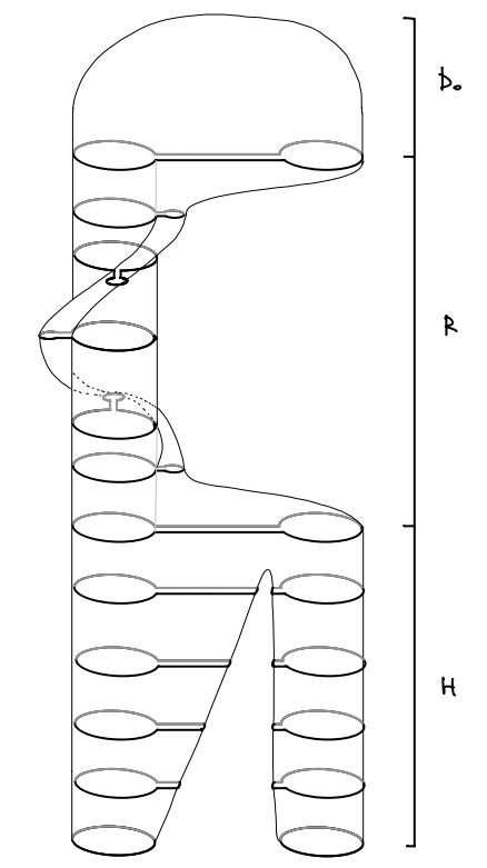
Let and be the trivial and roll-spun slice disks bounding respectively, viewed as cobordisms . Let denote the cobordism from to itself obtained as follows. First, shrink a ball containing and a small neighborhood of the attaching region for , small enough such that planar translations of the ball fit into the local pictures of around each crossing. Move the ball together with the attaching region along in accordance with the orientation of . Once the ball has traversed around once, enlarge the ball to its original position. The following observation was noted in [JZ20].
Lemma 2.
is isotopic to .
Proof.


Let denote the cobordism obtained by performing a -handle move at the band very near the attaching region for in the connected sum. To further simplify the cobordisms in hand, we consider and . The latter cobordism can be broken down into simpler cobordisms and , which admit Carter-Saito movie decompositions consisting only of Reidemeister II moves.

The cobordism is defined as follows. Here is an equivalent diagram of which will be described below. Replace the attaching region for in with a bump protruding towards , which we call a tentacle. Choose a ball containing and the tip of the tentacle, and move the ball along . Once the ball has traversed around once, we arrive at a link diagram that we denote by . Whenever the tentacle encounters a strand of , it moves under/over, depending on the under/over data on the corresponding crossing of . Hence can be decomposed into a movie consisting only of Reidemeister II moves.

The cobordism is then obtained by performing a -handle move between the tip of the tentacle, and the attaching region for in .

Finally, the cobordism is earned by moving the base of the tentacle along . Once the base traverses around once, we retrieve . Equivalently, is obtained by performing a series of Reidemeister II moves along the region formed between the tentacle and , and then performing a planar isotopy.

Lemma 3.
is isotopic to .
Proof.

4. Khovanov homology does not distinguish and
We assume that the diagram is chosen such that it has a minimal number of crossings. The presence of nugatory crossings complicates the proof of the main result, so we remove them from the onset to streamline the argument.
Theorem 3.
Khovanov homology fails to distinguish and viewed as cobordisms up to signs. More precisely, the maps
agree up to signs.
Corollary 1.
Let be a knot such that the -handle move is surjective. Then Khovanov homology fails to distinguish the trivial slice disk from the roll-spun slice disk viewed as cobordisms , up to signs.
In fact, we show that the equality already holds on the chain level by exploiting the observation that the generators of not mapped to zero under must take a particular form.
Let be a generator of . Write where are generators of . Consider a crossing in . Recall that is an oriented diagram, and without loss of generality assume that the crossing is arranged as in Figure 11. The over-and-under crossing data are irrelevant to the argument, and thus we suppress it in the figures.

The crossing could be resolved either by a -smoothing or an -smoothing in . Since the chain map associated to a Reidemeister II move preserves the smoothing data outside of the local picture on which the move is applied to, it follows that the choice of smoothing of in is equal to that of in . For ease of argument, let us label the crossings in the local picture around as in Figure 12.
Since the goal is to compute , we may ignore the generators that are mapped to zero under . This trick lets us cut down the number of generators we have to consider significantly, in light of the following lemma.

Lemma 4.
For each smoothing of a crossing in , there are only two possibilities for smoothings of nearby crossings of (as in Figure 12) in so that the generators are not mapped to under .
![[Uncaptioned image]](2607.16837v1/smoothing1.png)

Proof.
Suppose the crossing is resolved as in the top left corner of Figure 4. Recall that decomposes into a series of Reidemeister II moves. Inspecting such a Reidemeister move occurring around , we observe that must be resolved as in the top left corner of Figure 14 — otherwise it is killed by the Reidemeister II move, and hence .

Similarly, we inspect a Reidemeister II move of occuring around . As the tentacle of first enters the local picture through the horizontal strand of , it creates two crossings and . Recalling the effect of Reidemeister II moves on , we note that they must be smoothed as in the right of Figure 15. But as noticed in the previous argument, the bottom right smoothing is killed by . Hence must be resolved as in the top right corner of Figure 15.

Repeating this process for and , we observe that these crossings are forced to be smoothed as in the right of Figure 16.

Now there is a choice to make. The remaining crossings are not forced to be resolved in a particular manner. But if we choose a smoothing on a single crossing, say , the remaining three crossings are forced to be smoothed accordingly.

Indeed, repeating the process for the remaining crossings , , and , in that order, we see that the choice of smoothing on force these crossings to be smoothed in a particular way. See Figure 18 for the case when is assumed to be smoothed as in the left of Figure 17.

The case when is smoothed in the opposite manner is handled similarly. ∎
In fact, if one accounts for the smoothing data of two adjacent crossings in , we can further cut down the two possibilities to a single case. This will arise as a byproduct of the proof of the following lemmas. Before stating them, we introduce some notations.

Let and be two adjacent crossings in . Denote by the strand in between and . Let be a generator summand of . The portion of the tentacle along is split into two strands, either by another tentacle, or a strand in . Denote by the strand further away from . Note that is dependent on the summand . Choose a point in the intersection of all as ranges over the generator summands of . Clearly this intersection is nonempty.
We need the following definitions for later use.
Definition 3.
Let , where consists of the first Reidemeister II moves of , and the remaining Reidemeister II moves (in the canonical movie decomposition). Let be a generator summand of , and let be a point on the smoothing underlying that lies on a strand of bounded by two crossings and of . Let and be the strands of forming and together with , respectively.
We say that has traversed over through , if a tentacle of has crossed along . We say that has traversed along through , if a tentacle of has crossed along .

Note that our minimality assumption on the diagram of guarantees that , , and are all distinct.
Our goal is to show that a generator summand of , not killed by , must have the same label at as the component of containing . This is shown by repeatedly applying the following technical lemmas.
Lemma 5.
Decompose . Let be a generator summand of . If has a component labeled that lies between a strand of and the lower strand of a tentacle, then .
Proof.
We handle one case. Suppose has a component labeled configured as in the upper left corner of Figure 21. Note that does not leave the local picture, so we may assume that it stays labeled until the tentacle returns to the local picture. After a sequence of Reidemeister II moves in , the tentacle leaves the local picture, splitting into two components and .
The generator summands of can be grouped into two categories depending on how and are labeled. On one hand, we have summands whose and components are labeled and respectively (lower diagram in the upper right corner of Figure 21), and on the other hand we have summands labeled and respectively (upper diagram in the upper right corner of Figure 21). Let , be generator summands of in the first and second categories respectively.
Since and does not leave the local picture of Figure 21, in computing the effect of on and , we need only study the effect of a Reidemeister II move of occurring within the local picture. This is computed in the remainder of Figure 21, revealing that both and are zero.
The remaining cases (depending on the orientation and ordering of the strands in the local pictures) are handled analogously. ∎
![[Uncaptioned image]](2607.16837v1/kill1lemma.png)

Lemma 6.
Decompose , and let be a generator summand of . Then a component of completely encased between the two strands of a tentacle is labeled .
Proof.
We handle one case. Clearly we need only consider local pictures of as in the top left corner of Figure 22, and show that any component arising from further Reidemeister II moves that is completely encased within the two strands of a tentacle must be labeled . This is shown in Figures 22.
The remaining cases (depending on the orientation and ordering of the strands in the local pictures) are handled analogously. ∎
![[Uncaptioned image]](2607.16837v1/birth1lemma.png)

Iterating the above two principles yields the following technical results. We defer the proofs to the appendix.
Proposition 1.
Suppose that the component of containing is labeled . Let be a generator summand of not mapped to zero under . Then the component of containing is also labeled .
Lemma 7.
Let , , and be in Definition 3. Suppose has not traversed along . Decompose into , where is maximal among summands of consisting only of moves that do not traverse along . Suppose the component of containing is labeled . Then the component of containing is also labeled .
We also need analogous lemmas for in place of . The proofs are completely analogous.
Proposition 2.
Suppose that the component of containing is labelled . Let be a generator summand of not mapped to zero under . Then the component of containing is also labelled .
Lemma 8.
Let , , and be as in Lemma 7. Suppose has not traversed along . Decompose into , where is maximal among summands consisting only of moves that do not traverse along . Suppose the component of containing is labeled . Then the component of containing is also labeled .
Propositions 1 and 2 described the local labels when the strand in question is bounded by two crossings. To conclude the proof of the main result, we need to handle two exceptional cases. Namely, when the tentacle traverses the first crossing, and when the tentacle traverses the last crossing. These are taken care of by the following lemmas.
Lemma 9.
Let be a generator summand of such that . Let be a point of around the attaching region for the 1-handle . Then the labels of and at are the same.
Lemma 10.
Let , be points of , near the attaching region of the -handle . Let be a generator, and suppose that the component of containing is labeled , and the component containing is labeled . Let be a generator summand of not mapped to zero under . Then the component of containing the -handle is labeled .
Note that the component of containing the -handle is labeled as well.
Now we prove the main result. The argument will proceed by mimicking the proofs of Propositions 1 and 2 and Lemmas 7 and 8, but for the cobordism in place of .
Proof of Theorem 3.
Let be a generator summand of not mapped to zero under . The proofs of Propositions 1, 2 and Lemmas 9, 10 imply that the smoothing data of two adjacent crossings, and the label of the strand bounded by the crossings in , completely determine the generator summand. In particular, such a generator summand exists, and is unique.
By Lemmas 5 and 6, we know that every component of lying strictly between a strand of and the lower strand of the tentacle must be labeled , and that every component bounded within the tentacle must be labeled . We claim that up to signs, this forces to act by simply erasing the strand along and the bottom strand of the tentacle along while keeping the labels on the upper strand fixed. Since the intersections of the upper strands of tentacles are resolved and labeled in the same way as the corresponding crossings on , it follows from the claim that . The sign comes from the sign in the Reidemeister II move induced chain map on . More precisely, the sign counts the mod number of components of lying strictly between a strand of and a lower strand of the tentacle.
Hence we are reduced to proving the claim. Figures 25-29 and 32-36 force the local picture of around a strand of to fit into one of the eight cases described by Figures 62-63, provided that the strands are oriented as described (left vertical strand upwards, right vertical strand downwards). It suffices to show that the moves of keep the label at fixed. The verification of the claim for the first case, for moves of occurring in the local picture, is detailed in Figure 65. The verification for the remaining cases (for each choice of orientations and resolutions) are completely similar.
For moves of occurring outside the local picture, there are eight cases to consider for each choice of orientation and resolution, as described in Figures 66-67. The verification of the claim for the first case is detailed in Figure 68. Again, the verification for the remaining cases is completely similar. ∎
In light of Corollary 1, we end with the following interesting question. For which knots is the -handle map surjective?
Appendix
In this appendix we collect the proofs of the technical results in Section 4.
4.1. Proof of Propsition 1.
Suppose without loss of generality that is configured as in Figure 23. Decompose
where indicates the sequence of Reidemeiester II moves occurring in the local picture of , along the -th strand of , and indicates the sequence of interloping Reidemeister II moves of occurring outside the local picture.
We will later show in Lemma 7 that a generator summand of (for ) not killed by is labeled at , provided is labeled at . In light of this, we need only consider the action of on the local picture.
There are four ways to resolve the crossings and . In each case, Lemma 5 forces the generator summands of to take the form in Figure 24.
Now we consider the effect of on . To each of the four cases in Figure 24, there are two possible cases, depending on which of the two vertical strands are traversed first. The resulting computations are gathered in Figures 25-29. Note that these are the only orientations of the vertical strands we have to consider, since the tentacles associated to any other orientations would not interact with the strand . Also note that is labeled in every generator summand not killed by .
The effect of on can then be computed as follows. We apply the case when the left vertical strand is traversed first to the case when the right vertical strand is traversed first, by looking at the local picture of a strand bounded by the outer strand of a tentacle along the right vertical strand of , , and the left vertical strand of . This handles the case when the right vertical strand is traversed before the left vertical strand.
Vice versa, we can handle the remaining case when the left vertical strand is traversed before the right vertical strand. In fact, the two resulting local pictures are the same. i.e., there is no difference in the ordering of the strands when looking locally along .∎


![[Uncaptioned image]](2607.16837v1/localElemma2.png)

![[Uncaptioned image]](2607.16837v1/localElemma3.png)

![[Uncaptioned image]](2607.16837v1/localElemma4.png)

4.2. Proof of Proposition 2
The proof is completely analogous to that of Proposition 1, using Lemma 8 in place of Lemma 7. The relevant computations are detailed in Figures 30-36.∎


![[Uncaptioned image]](2607.16837v1/localElemmax2.png)

![[Uncaptioned image]](2607.16837v1/localElemmax3.png)

![[Uncaptioned image]](2607.16837v1/localElemmax4.png)

4.3. Proof of Lemma 7
By induction, it suffices to show that a strand labeled in that enters a local picture of a crossing stays labeled , after traverses over through the strand other than .
When is a strand of , there are six possible cases depending on how the crossing is resolved, and how the other strand is oriented. These are described in Figures 37-39. The configurations not belonging to these six cases can be ignored, since the tentacle would not interact with the component containing in the local picture. By rotating these figures and applying the appropriate computations in Figures 25-29, we can conclude that the tentacle along the horizontal strand of fixes the label at as well.
When is a strand of the tentacle, there are three possible cases, depending on how the crossing is smoothed, and whether belongs to the upper or the lower strand of the tentacle. These are handled in Figures 40-43. Again, configurations not described in these figures can be ignored.∎


4.4. Proof of Lemma 8
The proof is completely analogous to that of Lemma 7. The relevant computations are detailed in Figures 44-50.


4.5. Proof of Lemma 9
As described in Figure 51, there are four possible cases, depending on how the first crossing of is resolved in , and how is labeled. The computations detailed in Figures 52-59 verify the claim.∎


4.6. Proof of Lemma 10
Figure 60 describes the relevant local picture. There are two cases to consider, depending on how the last crossing of is resolved. Figure 61 verify the claim in each of these two cases. ∎


4.7. Figures for proof of the Theorem 3


![[Uncaptioned image]](2607.16837v1/localSlemma1.png)
![[Uncaptioned image]](2607.16837v1/localSlemma1_.png)
![[Uncaptioned image]](2607.16837v1/localSlemma1-1.png)
![[Uncaptioned image]](2607.16837v1/localSlemma1-1_.png)
![[Uncaptioned image]](2607.16837v1/localSlemma1_-1.png)


References
- [HS24] Kyle Hayden and Isaac Sundberg, Khovanov Homology and Exotic Surfaces in the 4-Ball, Journal Für Die Reine Und Angewandte Mathematik, 809 (2024), pp. 217–246.
- [Ja04] Magnus Jacobsson, An Invariant of Link Cobordisms from Khovanov Homology, Algebraic & Geometric Topology, 4 (2004), pp. 1211-1251.
- [JZ20] András Juhász and Ian Zemke, Distinguishing Slice Disks Using Knot Floer Homology. Selecta Mathematica, 26 (2020) no. 1, no. 5.
- [JM16] András Juhász and Marco Marengon, Concordance Maps in Knot Floer Homology, Geometry & Topology, 20 (2016), pp. 3623-3673.
- [Kh00] Mikhail Khovanov, A Categorification of the Jones Polynomial Duke Mathematical Journal, 101 (2000), pp. 359-426.
- [Li79] Richard A. Litherland, Deforming Twist-Spun Knots, Transactions of the American Mathematical Society, 250 pp. 311-331.
- [MWW22] Scott Morrison, Kevin Walker, Paul Wedrich, Invariants of 4-manifolds from Khovanov-Rozansky link homology, Geometry & Topology, 26 (2022) 250 pp. 3367-3420.