Two-dimensional solitons in extended GPE models with Lee-Huang-Yang corrections

We consider a homonuclear bosonic mixture whose components feature intracomponent repulsive 3D scattering lengths $a_{11}^{(3D)}=a_{22}^{(3D)}>0$ and an intercomponent attractive one, $a_{12}^{(3D)}<0$. The system is trapped in a 2D box, of length $L_{x}=L_{y}=L$, which can be experimentally achieved using digital-micromirror devices Saint-Jalm et al. (2019); Navon et al. (2021); Tamura et al. (2023) constraining the motion of the atoms in the $x$-$y$ plane and a tight transverse harmonic trap preventing excitations and pattern formation across the $z$-direction Hadzibabic and Dalibard (2011). In a corresponding experiment, this composition can be realized, for instance, by the hyperfine states $\ket{1}\equiv\ket{F=1,m_{F}=-1}$ and $\ket{2}\equiv\ket{F=1,m_{F}=0}$ of ³⁹K Cabrera et al. (2018). Accordingly, the individual 2D scattering lengths, $a_{11},a_{22},a_{12}$, depend on the corresponding 3D ones Petrov and Shlyapnikov (2001); Bougas et al. (2024), which are in turn tunable via Fano-Feshbach resonances Chin et al. (2010); Cheiney et al. (2018); Cabrera et al. (2018). Throughout this work, we operate in the scattering length interval where the distance from the mean-field balance point $\delta a\equiv a_{12}+\sqrt{a_{11}a_{22}}\lesssim 0$. This refers to the magnetic field region $B\sim 57$G of ³⁹K D’Errico et al. (2007); Tanzi et al. (2018) in which quantum droplets exist Luo et al. (2021); Petrov and Astrakharchik (2016).

The above condition on the intracomponent scattering lengths ($a_{11}=a_{22}=a$), along with the consideration of equal atom number per component ($N_{1}=N_{2}$), suffice to reduce²²2Alternatively, this reduction is ensured through $\left|\psi_{1}\right|^{2}/\left|\psi_{2}\right|^{2}=\sqrt{a_{22}}/\sqrt{a_{11}}$ Petrov and Astrakharchik (2016); Petrov (2015); Semeghini et al. (2018). the two-component system into an effective single-component one Petrov and Astrakharchik (2016) describing a symmetric droplet with 2D wave functions $\psi_{1}(x,y,t)=\psi_{2}(x,y,t)\equiv\psi(x,y,t)$. The underlying 2D eGPE Petrov and Astrakharchik (2016) reads

$$i\hbar\psi_{t}=-\frac{\hbar^{2}}{2m}\Delta\psi+\frac{8\pi\hbar^{2}n_{0}\sqrt{e}}{m\ln^{2}(a_{12}/a)}|\psi|^{2}\psi\ln\big(|\psi|^{2}\big),$$

(1)

and is supplemented with the boundary condition

$$\quad|\psi|\rightarrow|\psi_{0}|={\rm const.},\quad\text{as}\quad\|\mathbf{r}\|\rightarrow\infty$$

. In Eq. (1), $n_{0}$ denotes the equilibrium density of the droplet in the thermodynamic limit Petrov and Astrakharchik (2016), $m$ is the atomic mass, and $\Delta$ represents the 2D Laplacian. Below, we employ both Cartesian and cylindrical coordinates, where $\mathbf{r}=(x,y)$ and $\mathbf{r}=(r,\theta)$ respectively, since they will be both used for our analytical considerations in Sec. III, IV. Accordingly, the 2D Laplacian is given by $\Delta=\partial_{x}^{2}+\partial_{y}^{2}$, and $\Delta=(1/r)\partial_{r}(r\partial_{r})+(1/r^{2})\partial_{\theta}^{2}$ respectively.

Measuring the time $t$, the spatial coordinates $x$ and $y$, and wavefunction $\psi(\mathbf{r},t)$ in units $m/\hbar n_{0}$, $n_{0}^{-1/2}$ and $\sqrt{n_{0}\sqrt{e}}$, respectively, we cast Eq. (1) in the following dimensionless form

$$i\psi_{t}+\frac{1}{2}\Delta\psi-g|\psi|^{2}\psi\ln\big(|\psi|^{2}\big)=0,$$

(2)

where the effective interaction strength $g=8\pi\sqrt{e}/(\ln^{2}(a_{12}/a))$ Petrov and Astrakharchik (2016); Bougas et al. (2024). Notice that the logarithmic nonlinearity appearing in the 2D eGPE encapsulates both the standard mean-field interactions and the LHY term. Moreover, at low densities the negativity of the logarithm yields attractive interactions, in contrast to large densities where the logarithm is positive and repulsive interactions dominate.

To numerically study (see below) the evolution of the 2D solitons on top of the droplet background, we utilize the time-dependent 2D eGPE of Eq. (2). Specifically, a fourth-order Runge-Kutta integrator supplemented by a second-order finite differences method (cross-validated with a pseudospectral method) to compute the spatial derivatives is deployed. The spatial and temporal discretizations in our simulations refer to $dx=dy=0.08$ and $dt=10^{-4}$ respectively. Additionally, homogeneous Neumann boundary conditions suitable for the asymptotics of the 2D line, lump, ring solitons and dromion are used, notably due to the finite density of the associated background. Typical box sizes $L=200$ within our dimensionless units translate to $65~\rm{\mu m}$, whilst evolution times of the order of $t\sim 200$ correspond to $14~\rm{ms}$ for transverse oscillator length $a_{z}=0.11~\rm{\mu m}$ with $\omega_{z}=2\pi\times 20~\rm{kHz}$.

We now introduce the Madelung transformation

$$\psi(\mathbf{r},t)=\sqrt{\rho(\mathbf{r},t)}\,e^{i\phi(\mathbf{r},t)},$$

(3)

where $\rho(\mathbf{r},t)$ and $\phi(\mathbf{r},t)$ denote the density and phase, respectively. Substituting Eq. (3) into Eq. (2), and separating real and imaginary parts, we obtain the following hydrodynamical system

	$\displaystyle\rho_{t}+\nabla\cdot(\rho\nabla\phi)=0,$		(4a)
	$\displaystyle\phi_{t}+\frac{1}{2}\|\nabla\phi\|^{2}-\frac{1}{2}\rho^{-1/2}\Delta\rho^{1/2}+g\rho\ln\rho=0.$		(4b)

The above equations possess the following elementary nontrivial solution,

$$\rho(\mathbf{r},t)=\rho_{0}={\rm const.},\quad\phi(\mathbf{r},t)=-\mu t,$$

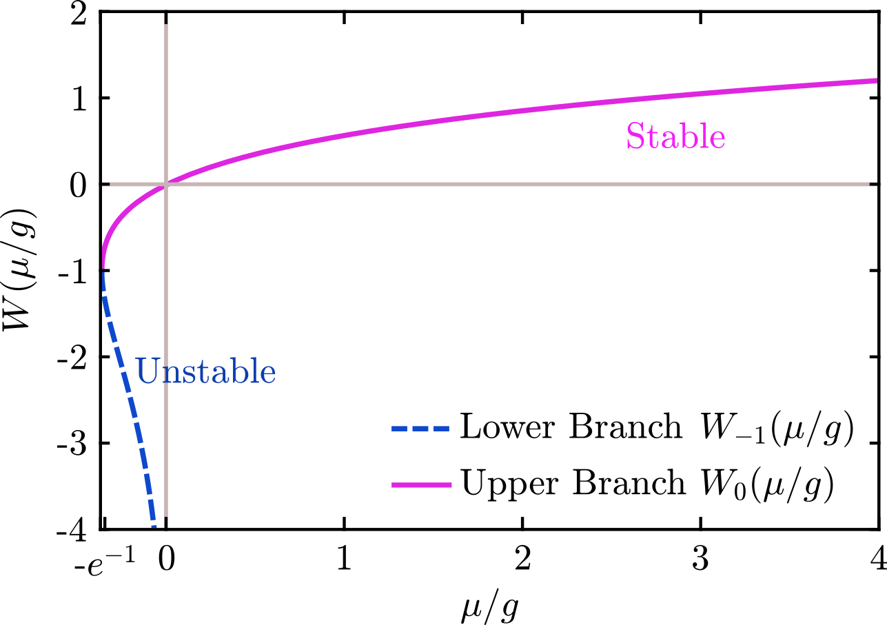
where $\mu=g\rho_{0}\ln(\rho_{0})$ is the chemical potential. It can readily be found that the background density $\rho_{0}$ and the chemical potential $\mu$ are connected through the following equation,

$$\rho_{0}=\frac{\mu/g}{W\!\left(\mu/g\right)},$$

(5)

where $W$ is the Lambert $W$-function, namely the inverse function of $f(W)=W\exp(W)$. As shown in Fig. 1, and similarly to the 1D case Katsimiga et al. (2023), there exist two branches: the upper (principal) branch, $W_{0}(\mu/g)$, and the lower branch $W_{-1}(\mu/g)$, of the Lambert W-function. The upper branch exists for chemical potentials $\mu>\mu_{c}$, where the critical value $\mu_{c}=-ge^{-1}$, while the lower branch exists for $-e^{-1}\leq\mu/g\leq 0$.

Next, we consider the stability of the homogeneous background solution. Substituting the Ansatz

$$\rho=\rho_{0}+\varepsilon\rho_{1}(\mathbf{r},t),\qquad\phi=-\mu t+\varepsilon\phi_{1}(\mathbf{r},t),$$

into Eqs. (4a)-(4b), where $0<\varepsilon\ll 1$ is a small parameter, we obtain at $\mathcal{O}(\varepsilon)$ the following linear system for the unknown functions $\rho_{1}$ and $\phi_{1}$:

	$\displaystyle\rho_{1t}+\rho_{0}\Delta\phi_{1}=0$		(6a)
	$\displaystyle\phi_{1t}-\frac{1}{4\rho_{0}}\Delta\rho_{1}+g(1+\ln\rho_{0})\rho_{1}=0.$		(6b)

The compatibility condition of Eqs. (6a)-(6b), $\partial_{t}\Delta\phi_{1}=\Delta\phi_{1t}$, yields

$$\rho_{1tt}-c^{2}\,\Delta\rho_{1}+\frac{1}{4}\,\Delta^{2}\rho_{1}=0,$$

(7)

where $c^{2}=g\rho_{0}(1+\ln\rho_{0})=\mu\left[1+1/(W(\mu/g))\right]$. Obviously, Eq. (7) is either hyperbolic, for $c^{2}>0$, or elliptic, for $c^{2}<0$. It can readily be seen that the hyperbolic (elliptic) case corresponds to the upper (lower) branch of the Lambert $W$-function. As a result, plane wave solutions, of the form $\rho_{1}\propto\exp[i(\mathbf{k}\cdot\mathbf{r}-\omega t)]$ (where $\mathbf{k}$ and $\omega$ are the wave vector and frequency of the perturbation) are either modulationally stable or unstable, for the upper or the lower branch of $W(\mu/g)$. Indeed, Eq. (7) leads to the Bogoliubov dispersion relation

$$\omega^{2}=c^{2}\|\mathbf{k}\|^{2}+\frac{1}{4}\|\mathbf{k}\|^{4},$$

(8)

with $\omega\in\mathbb{R}~~\forall\|k\|\in\mathbb{R}$ for $c^{2}>0$, i.e., for the upper branch, $W_{0}(\mu/g)$, of the Lambert $W$-function. The lower branch is the one that engenders the presence of 2D quantum droplets that are, arguably, the prototypical structures studied in the context of the model of Eq. (2) Luo et al. (2021). Our focus in the present work will shift away from that setting: indeed, we will seek 2D weakly nonlinear excitations (i.e., solitons) on top of the modulationally stable background. These will involve structures that asymptote to non-vanishing boundary conditions (contrary to the vanishing boundary conditions associated with the droplets).

Next, we consider the weakly nonlinear regime. First, we show that Eq. (2) can be asymptotically reduced to a completely integrable 2D system, namely the KP-I equation. We seek solutions of Eqs. (4a)-(4b) in the form of the following asymptotic expansions:

	$\displaystyle\rho$	$\displaystyle=$	$\displaystyle\rho_{0}+\varepsilon\rho_{1}+\varepsilon^{2}\rho_{2}+\cdots,$		(9a)
	$\displaystyle\phi$	$\displaystyle=$	$\displaystyle-\mu t+\varepsilon^{1/2}\phi_{1}+\varepsilon^{3/2}\phi_{2}+\cdots,$		(9b)

where the unknown functions $\rho_{j}$, $\phi_{j}$ ($j=1,2,\ldots$) depend on the stretched variables

$$X=\varepsilon^{1/2}(x-Ct),\quad Y=\varepsilon y,\quad T=\varepsilon^{3/2}t,$$

for the Cartesian case, or

$$R=\varepsilon^{1/2}(r-Ct),\qquad\Theta=\varepsilon^{-1/2}\theta,\qquad T=\varepsilon^{3/2}t,$$

for the polar coordinates; here, $C$ is an unknown velocity, to be determined in a self-consistent manner. Substituting Eq. (9a) and (9b) into Eqs. (4a)-(4b) we obtain

	$\displaystyle-c\rho_{j\mathcal{X}}+\rho_{0}\phi_{j\mathcal{X}\mathcal{X}}=P_{j}^{(C,p)},$		(10a)
	$\displaystyle-c\phi_{j\mathcal{X}}+g(1+\ln\rho_{0})\rho_{j}=Q_{j}^{(C,p)},$		(10b)

where $\mathcal{X}=X$, $P_{j}^{(C,p)}\equiv P_{j}^{(C)}$, $Q_{j}^{(C,p)}\equiv Q_{j}^{(C)}$ for the Cartesian case, and $\mathcal{X}=R$, $P_{j}^{(C,p)}\equiv P_{j}^{(p)}$, $Q_{j}^{(C,p)}\equiv Q_{j}^{(p)}$ for the polar case. For $j=1$, i.e., at $\mathcal{O}(\varepsilon)$, the above system is homogeneous, namely $P_{1}=Q_{1}=0$. In this case, combining Eqs. (10a)-(10b) we find

$$\left[-C^{2}+g\rho_{0}(1+\ln\rho_{0})\right]\rho_{j\mathcal{X}}=0,$$

(11)

which, for $\rho_{j\mathcal{X}}\neq 0$, leads to the compatibility condition $C^{2}=g\rho_{0}(1+\ln\rho_{0})$. This result shows that $C\equiv c$, as was obtained in Sec. II.2 [see Eq. (8)]. Furthermore, at $\mathcal{O}(\varepsilon)$, we obtain the following equation that connects the functions $\phi_{1}$ and $\rho_{1}$:

$$\phi_{1\mathcal{X}}=\frac{c}{\rho_{0}}\rho_{1}.$$

(12)

For $j>1$, the system of Eqs.  (10a)-(10b) is inhomogeneous, i.e., $P_{j}^{(C,p)}\neq 0$, $Q_{j}^{(C,p)}\neq 0$. In this case, combining Eqs. (10a)-(10b) we obtain

$$\left[-c^{2}+g\rho_{0}(1+\ln\rho_{0})\right]\rho_{j\mathcal{X}}=cP_{j}^{(C,p)}+\rho Q_{j\mathcal{X}}^{(C,p)},$$

(13)

and, thus, the compatibility condition is

$$cP_{j}^{(C,p)}+\rho Q_{j\mathcal{X}}^{(C,p)}=0.$$

(14)

First, we consider the Cartesian case. For $j=2$, the functionals $P_{2}^{(C)}$ and $Q_{2}^{(C)}$ are

	$\displaystyle P_{2}^{(C)}$	$\displaystyle=$	$\displaystyle-\rho_{1T}-\left(\rho_{1}\phi_{1X}\right)_{X}-\rho_{0}\phi_{1YY},$		(15a)
	$\displaystyle Q_{2}^{(C)}$	$\displaystyle=$	$\displaystyle-\phi_{1T}-\frac{1}{2}\phi_{1X}^{2}-\frac{g}{2\rho_{0}}\rho_{1}^{2}+\frac{1}{4\rho_{0}}\rho_{1XX}.$		(15b)

Substituting Eqs. (15a)-(15b) into Eq. (14), and using Eq. (12), we obtain the following KP-I equation:

$$\Big[\rho_{1T}-\frac{1}{8c}\rho_{1XXX}+\frac{g}{2c}(4+3\ln\rho_{0})\rho_{1}\rho_{1X}\Big]_{X}+\frac{c}{2}\rho_{1YY}=0.$$

(16)

Using the transformations

$$T\mapsto-8cT,\quad Y\mapsto c\sqrt{\frac{4}{3}}Y,\quad\rho_{1}\mapsto-\frac{2}{3}g(4+3\ln\rho_{0})\rho_{1},$$

we express Eq. (16) in the standard form of the KP-I equation,

$$\left(\rho_{1T}+6\rho_{1}\rho_{1X}+\rho_{1XXX}\right)_{X}-3\rho_{1YY}=0.$$

(17)

Next, we proceed with the polar case. For $j=2$, the functionals $P_{2}^{(p)}$ and $Q_{2}^{(p)}$ are

	$\displaystyle P_{2}^{(p)}$	$\displaystyle=$	$\displaystyle-\rho_{1T}-\left(\rho_{1}\phi_{1R}\right)_{R}-\frac{\rho_{0}}{cT}\phi_{1R}-\frac{\rho_{0}}{c^{2}T^{2}}\phi_{1\Theta\Theta},$
	$\displaystyle Q_{2}^{(p)}$	$\displaystyle=$	$\displaystyle-\phi_{1T}-\frac{1}{2}\phi_{1R}^{2}-\frac{g}{\rho_{0}}\rho_{1}^{2}+\frac{1}{4\rho_{0}}\rho_{1RR}.$		(18b)

As in the Cartesian case, we substitute Eqs. (LABEL:p1p)-(18b) into Eq. (14), and employing Eq. (12), we derive the following, so-called, cylindrical KP-I (cKP-I), or Johnson’s Johnson (1980) equation:

	$\displaystyle\Big[\rho_{1T}-\frac{1}{8c}\rho_{1RRR}+\frac{g}{2c}(4+3\ln\rho_{0})\rho_{1}\rho_{1R}+\frac{1}{2T}\rho_{1}\Big]_{R}$
	$\displaystyle+\frac{1}{2cT^{2}}\rho_{1\Theta\Theta}=0.$		(19)

Using the transformations

$\displaystyle R\mapsto-\frac{R}{(8c)^{1/3}},\,\,\,\Theta\mapsto\frac{\Theta}{2\sqrt{3}c^{2/3}},\,\,\,\rho_{1}\mapsto-\frac{6c^{2/3}\rho_{1}}{g(4+3\ln\rho_{0})},$

the cKP-I (19) is expressed in its standard form,

$$\left(\rho_{1T}+6\rho_{1}\rho_{1R}+\rho_{1RRR}+\frac{1}{2T}\rho_{1}\right)_{R}-\frac{3}{T^{2}}\rho_{1\Theta\Theta}=0.$$

(20)

In the following, we will show that Eq. (2) can be asymptotically reduced to another 2D completely integrable system, namely the DS-I system. To do so, we consider the Cartesian case, and seek solutions of Eqs. (4a)-(4b) in the form of the asymptotic expansions

	$\displaystyle\rho$	$\displaystyle=$	$\displaystyle\rho_{0}+\varepsilon\rho_{1}+\varepsilon^{2}\rho_{2}+\cdots,$		(21a)
	$\displaystyle\phi$	$\displaystyle=$	$\displaystyle-\mu t+\varepsilon\phi_{1}+\varepsilon^{2}\phi_{2}+\cdots,$		(21b)

where the unknown functions $\rho_{j}$, $\phi_{j}$ ($j=1,2,\ldots$) depend on the stretched variables

$$\theta=kx-\omega t,\,X=\varepsilon^{1/2}(x-Vt),\ Y=\varepsilon y,\ T=\varepsilon^{3/2}t,$$

where $V$ is an unknown velocity, to be determined. Substituting the expansions into Eqs. (4a)-(4b) and equating coefficients of like powers of $\varepsilon$, we obtain the coupled set of equations,

	$\displaystyle-\omega\,\rho_{j\theta}+k^{2}\rho_{0}\,\phi_{j\theta\theta}=F_{j},$		(22a)
	$\displaystyle-\dfrac{k^{2}}{4\rho_{0}}\rho_{j\theta\theta}-\omega\,\phi_{j\theta}+g\rho_{j}(1+\ln\rho_{0})=G_{j},$		(22b)

for $j=1,2,\ldots$. Notice that, eliminating $\phi_{j}$, the above system reduces to the following equation for $\rho_{j}$:

$$-\frac{1}{4}k^{2}\rho_{j\theta\theta\theta}+\left[g\rho_{0}(1+\ln\rho_{0})k^{2}-\omega^{2}\right]\rho_{j\theta}=\omega F_{j}+\rho_{0}k^{2}G_{j\theta}.$$

(23)

Below we focus on the first three orders of approximation, for which the above system leads to the following results.

To leading order, $\mathcal{O}(\varepsilon)$ ($j=1$), the system is linear and homogeneous ($F_{1}=G_{1}=0$), and yields the dispersion relation for the wavenumber $k$ and frequency $\omega$,

$\displaystyle\omega^{2}=c^{2}k^{2}+\frac{1}{4}k^{4},$

(24)

where $c^{2}=g\rho_{0}(1+\ln\rho_{0})$ as expected. Note that Eq. (24) is identical to Eq. (8) for $k_{x}=k$ and $k_{y}=0$. Additionally, at $\mathcal{O}(\varepsilon)$, the leading-order solution for $\rho_{1},\phi_{1}$ reads:

$\displaystyle\begin{cases}\rho_{1}=\displaystyle i\frac{k^{2}\rho_{0}}{\omega}\,q(X,Y,T)e^{i\theta}+{\rm c.c.},\\[5.69054pt] \phi_{1}=q(X,Y,T)e^{i\theta}+{\rm c.c.}+\Phi(X,Y,T),\end{cases}$

(25)

where c.c. denotes complex conjugate. In the above expressions, $q$ denotes the unknown complex envelope of the carrier wave $\exp(i\theta)$, while $\Phi$ is a long-wavelength mean flow term (corresponding to $k=0$). Both $q$ and $\Phi$ depend solely on the slow variables $X$, $Y$ and $T$ and, as will be shown below, these unknown functions satisfy the DS system.

Proceeding to the next order $\mathcal{O}(\varepsilon^{2})$ ($j=2$), the system becomes inhomogeneous, with the right-hand side terms given by:

	$\displaystyle F_{2}$	$\displaystyle=$	$\displaystyle c\rho_{1X}-k^{2}\rho_{1\theta}\phi_{1\theta}-2k\rho_{0}\phi_{1\theta X}-k^{2}\rho_{1}\phi_{1\theta\theta},$
	$\displaystyle G_{2}$	$\displaystyle=$	$\displaystyle-\frac{g}{2\rho_{0}}\rho_{1}^{2}+c\phi_{1X}-\frac{k^{2}}{8\rho_{0}^{2}}\rho_{1\theta}^{2}$
		$\displaystyle-$	$\displaystyle\frac{k^{2}}{2}\phi_{1\theta}^{2}+\frac{k}{2\rho_{0}}\rho_{1\theta X}-\frac{k^{2}}{4\rho_{0}^{2}}\rho_{1}\rho_{1\theta\theta}.$

The solvability condition for Eq. (23) at this order, obtained upon removing the secular terms $\propto\mathrm{exp}(i\theta)$, yields the unknown velocity $V$. The latter is found to be the group velocity $v:=d\omega/dk$, as can be obtained from the dispersion relation (24). In this way, we find

$\displaystyle V\equiv v=\frac{k^{3}}{4\omega}+\frac{\omega}{k}.$

(27)

Moreover, at $\mathcal{O}(\varepsilon^{2})$, we obtain the following expressions for the unknown fields $\rho_{2},\phi_{2}$:

$\displaystyle\begin{cases}\rho_{2}=\bigl(a_{1}q^{2}e^{2i\theta}+a_{2}q_{X}e^{i\theta}+\text{c.c.}\bigr)+a_{3}|q|^{2}+a_{4}\,\Phi_{X},\\ \phi_{2}=a_{5}q^{2}e^{2i\theta},\end{cases}$

(28)

where the coefficients $a_{j}$ ($j=1,2,\ldots 5$) are given in Appendix A.

Finally, at the order $\mathcal{O}(\varepsilon^{3})$, the right-hand side terms of the system are given by

	$\displaystyle F_{3}$	$\displaystyle=$	$\displaystyle-\rho_{1T}-\rho_{0}\phi_{1YY}+c\rho_{2X}-\rho_{0}\phi_{1XX}-k\phi_{1X}\rho_{1\theta}$
		$\displaystyle-$	$\displaystyle k\rho_{1X}\phi_{1\theta}-k^{2}\rho_{2\theta}\phi_{1\theta}-k^{2}\rho_{1\theta}\phi_{2\theta}-2k\rho_{1}\phi_{1\theta X}$
		$\displaystyle-$	$\displaystyle 2\rho_{0}k\phi_{2\theta X}-k^{2}\rho_{2}\phi_{1\theta\theta}-k^{2}\rho_{1}\phi_{2\theta\theta},$
	$\displaystyle G_{3}$	$\displaystyle=$	$\displaystyle\frac{g}{6\rho_{0}^{2}}\rho_{1}^{3}-\frac{g}{\rho_{0}}\rho_{1}\rho_{2}-\phi_{1T}+\frac{1}{4\rho_{0}}\rho_{1YY}+c\phi_{2X}$
		$\displaystyle+$	$\displaystyle\frac{1}{4\rho_{0}}\rho_{1XX}-\frac{k}{4\rho_{0}^{2}}\rho_{1X}\rho_{1\theta}+\frac{k^{2}}{4\rho_{0}^{3}}\rho_{1}\rho_{1\theta}^{2}-\frac{k^{2}}{4\rho_{0}^{2}}\rho_{1\theta}\rho_{2\theta}$
		$\displaystyle-$	$\displaystyle k\phi_{1X}\phi_{1\theta}-k^{2}\phi_{1\theta}\phi_{2\theta}-\frac{k}{2\rho_{0}^{2}}\rho_{1}\rho_{1\theta X}+\frac{k}{2\rho_{0}}\rho_{2\theta X}$
		$\displaystyle+$	$\displaystyle\frac{k^{2}}{4\rho_{0}^{3}}\rho_{1}^{2}\rho_{1\theta\theta}-\frac{k^{2}}{4\rho_{0}^{2}}\rho_{2}\rho_{1\theta\theta}-\frac{k^{2}}{4\rho_{0}^{2}}\rho_{1}\rho_{2\theta\theta}.$

At this order, the solvability condition is derived upon removing again the secular terms, which are now $\propto\exp(i\theta)$ and $\propto\exp(i0\theta)=1$ (constant terms). This way, we obtain the following set of two-coupled equations for the unknown fields $q$ and $\Phi$:

	$\displaystyle ic_{0}q_{T}+c_{1}q_{XX}+c_{2}q_{YY}+\bigl(c_{3}|q|^{2}+c_{4}\Phi_{X}\bigr)q=0,\hskip 28.45274pt$		(30a)
	$\displaystyle c_{5}\Phi_{XX}+c_{6}\Phi_{YY}+c_{7}(|q|^{2})_{X}=0,\hskip 28.45274pt$		(30b)

where the coefficients $c_{j}$ ($j=0,1,\ldots,7$) are functions of $k$. The form of these coefficients, in the long-wavelength limit, are provided in Appendix A.

The system of Eqs. (30a)-(30b) has been used to describe modulated multidimensional water waves in finite depth. This model was first derived by Benney and Roskes (BR) Benney and Roskes (1969), then by Davey and Stewartson (DS) Davey and Stewartson (1974), and also by Djordjevic and Redekopp (DR) Djordjevic and Redekopp (1977), who included surface tension. In its general form the BR/DR system is not integrable. Nevertheless, in the shallow water limit ($kH\rightarrow 0$, where $k$ is the wavenumber and $H$ is the water’s depth), Ablowitz and Segur Ablowitz and Segur (1979) derived the completely integrable version, known as the DS system.

To derive the nearly integrable version of Eqs. (30a)-(30b) we proceed as follows. First, we introduce the transformations

	$\displaystyle X\mapsto\sqrt{\left|\frac{c_{0}}{c_{1}}\right|}\,X,\qquad~~Y\mapsto\sqrt{\left|\frac{c_{0}}{c_{2}}\right|}\,Y,$
	$\displaystyle|q|^{2}\mapsto 2A\left|\frac{c_{0}}{c_{3}}\right|\,|q|^{2},\quad\varphi\mapsto-\frac{c_{0}}{c_{4}}\,\varphi,$

where the parameter $A$ is given by

$$A=-\frac{2+\ln\rho_{0}}{8+6\ln\rho_{0}},$$

and then express Eqs. (30a)-(30b) in the following normalized form:

	$\displaystyle iq_{T}+q_{XX}+q_{YY}-|q|^{2}q-\varphi q=R[q],$		(31a)
	$\displaystyle\varphi_{XX}-\varphi_{YY}+2(|q|^{2})_{XX}=0,$		(31b)

where $\varphi=\Phi_{X}$ and the functional perturbation $R[q]$ is given by

$$R[q]=-\left(1+2A\right)|q|^{2}q.$$

In the case $R[q]=0$, the system of Eqs.  (31a)-(31b) takes the form of the completely integrable DS-I system; note that in DS-I, Eq. (31a) [Eq. (31b)] is elliptic (hyperbolic) as concerns the 2nd derivative operator in $q$ ($\varphi$). In such a case, the DS-I system supports exact analytical 2D soliton solutions, known as dromions, which will be presented in Sec. IV.3. Such solutions are still physically relevant in the case where the functional $R[q]$ may be considered as a small perturbation for values of the background density $\rho_{0}\gtrsim e^{-1}$ or chemical potential $\mu\gtrsim-ge^{-1}$, i.e., close to the critical value $\mu_{c}$. This in turn implies that the dromion for any $\mu>-ge^{-1}$ is an approximate solution and, as such, it is expected that it will deviate the most from the numerical predictions; see also the discussion in Sec. IV.3 and Fig. 7.

Starting with the KP-I soliton solutions in the Cartesian case, there exist two physically important types of soliton solutions, namely line and lump solitons. The single line soliton of the KP-I equation, expressed in the original coordinates $x$, $y$, $t$, reads

	$\displaystyle\rho_{1}$	$\displaystyle=$	$\displaystyle-\frac{3\kappa_{1}^{2}}{g(4+3\ln\rho_{0})}{\rm sech}^{2}\xi,$		(32a)
	$\displaystyle\xi$	$\displaystyle=$	$\displaystyle\varepsilon^{1/2}\kappa_{1}\Bigg[x-c\left(1-\varepsilon\frac{4\kappa_{1}^{2}-3\kappa_{2}^{2}}{8c^{2}}\right)t$		(32b)
		$\displaystyle+$	$\displaystyle\varepsilon^{1/2}\frac{\sqrt{3}\kappa_{2}}{2c}y\Bigg]-\xi_{0},$

where $\kappa_{1}$ and $\kappa_{2}$ are arbitrary $\mathcal{O}(1)$ parameters, and $\xi_{0}$ sets the initial soliton location. We remark that line soliton solutions or their traveling gray soliton variants Katsimiga et al. (2023) are also expected to exist in the corresponding effective 1D eGPE model featuring logarithmic nonlinearity Mistakidis et al. (2025). This approach would lift one level of approximation and it is an interesting future research direction.

On the other hand, the KP-I equation possesses weakly localized 2D soliton solutions, decaying algebraically at infinity. These solutions are known as lumps Ablowitz and Clarkson (1991); indeed, the line solitons of KP-I are transversely unstable toward the formation of the lumps. The one-lump soliton solution, expressed in the original variables $x,y,t$, is given by the following rational expression:

$$\!\!\!\!\rho_{1}=-\frac{6}{g\,(4+3\ln\rho_{0})}\frac{-(x^{\prime}+\lambda_{1}y^{\prime})^{2}+\lambda_{2}^{2}y^{\prime 2}+\frac{1}{\lambda_{2}^{2}}}{\left[(x^{\prime}+\lambda_{1}y^{\prime})^{2}+\lambda_{2}^{2}y^{\prime 2}+\frac{1}{\lambda_{2}^{2}}\right]^{2}},$$

(33)

where $\lambda_{1}$ and $\lambda_{2}$ are arbitrary $\mathcal{O}(1)$ parameters, and the variables $x^{\prime}$ and $y^{\prime}$ are given by:

	$\displaystyle x^{\prime}$	$\displaystyle=$	$\displaystyle\varepsilon^{1/2}\left\{x-\left[c-\varepsilon\frac{3}{8c}(\lambda_{1}^{2}+\lambda_{2}^{2})\right]t\right\},$		(34a)
	$\displaystyle y^{\prime}$	$\displaystyle=$	$\displaystyle\varepsilon\frac{\sqrt{3}}{2c}\left(y-\varepsilon^{1/2}\frac{\sqrt{3}}{2}\lambda_{1}t\right).$		(34b)

The above expressions for the line and the lump solitons can be used to construct pertinent approximate soliton solutions —valid up to $\mathcal{O}(\varepsilon)$— of the original problem of Eq. (2),

	$\displaystyle\!\!\!\!\!\psi$	$\displaystyle\approx$	$\displaystyle[\rho_{0}+\varepsilon\rho_{1}(x,y,t)]^{1/2}$		(35)
		$\displaystyle\times$	$\displaystyle\exp\left[-{\rm i}\mu t+{\rm i}\varepsilon^{1/2}\frac{c}{\rho_{0}}\int^{X}\rho_{1}(X^{\prime},y,t){\rm d}X^{\prime}\right].$

The density evolution of a relatively shallow 2D line soliton, as obtained from the approximate KP-I solution of Eq. (32a), on top of the droplet background is depicted in Fig. 3. Inspecting the 2D density profiles in Fig. 3(a)-(e), it becomes apparent that the structure is a dark (grey) soliton stripe, of the form of a density depletion localized along the propagation $x$-direction, and being elongated transversely. It is also characterized by a phase jump $\rm{Arg}[\psi(x,0)]\approx\pi/4$ [Fig. 3(f)] across its core, which is smaller than $\pi$ (that corresponds to a stationary (black) soliton) due to its shallow depth. The soliton moves to the right, preserving its shape, while emitting a small amount of radiation (subsequently propagating on the homogeneous background) traced back to the approximate nature of the solution. The aforementioned radiation occurs in both right and left $x$-directions, while it clearly manifests as small amplitude oscillatory patterns on the droplet background identified in the corresponding density profiles across the $x$ axis at $y=0$ illustrated in Fig. 3(f)-(j). Additionally, the depth and phase jump of the moving line soliton reduce slightly in the course of the evolution, see Fig. 3(f)-(j). This confirms the validity of the asymptotic reduction to the KP-I model in the modulational stable droplet environment. Nonetheless, the line soliton structure is persistent over long times without suffering significant distortions, thereby suggesting its dynamical stability and, hence, the feasibility to observe this solitary wave in 2D droplet systems.

Turning to the dynamics of the 2D lump soliton described by Eq. (33), we observe a somewhat more involved response [Fig. 4] as compared to the previously discussed straight line soliton. Indeed, as time evolves the lump which is a strongly localized density depression with algebraic spatial decay moves to the left [Fig. 4(a)-(e)], while experiencing a slight gradual broadening of its core and becoming noticeably less deep, see in particular the 1D density profiles in Fig. 4(f)-(j). This process, being more prominent when compared to the line soliton propagation, is naturally accompanied by a reduction of the initial small phase jump across its core, i.e., $\rm{Arg}[\psi(x,0)]\approx\pi/4$, due to the shallow character of the structure. In sharp contrast to the line soliton, the initially symmetric localized lump soliton profile develops a slight curvature, indicating the deformation of its shape during the evolution. This behavior, along with the simultaneous development of small amplitude radiation is a result of the approximate character of the analytical solution in the 2D eGPE model. Summarizing, the robustness of the localized lump configuration as time progresses validates the relevance of the KP-I lump solution for describing 2D solitary waves in quantum droplet environments, while the observed deformations highlight the important role of non-integrable effects in long-time dynamics.

An interesting connection between the line and the lump solitons can also be established through the transverse destabilization of the former, as it was also discussed in polariton superfluids Frantzeskakis et al. (2018). To demonstrate this behavior in the current droplet setting we slightly modify the core of the line soliton by perturbing it along the $y$-direction through $x\to x-A\cos(Ky)$ where $A=0.5$ and $K=0.25$. The ensuing density dynamics of the perturbed line soliton within the eGPE framework is shown in Fig. 5(a)-(e) along with the associated phase profiles in Fig. 5(f)-(j). It can be readily seen that as time evolves the line soliton moves to the left with the azimuthal perturbation becoming more pronounced.

As a result, noticeable spatial deformations develop on top of the line waveform eventually leading to its dissolvement into an array of lump solitons [Fig. 5(c)-(e)] with a characteristic phase structure shown in Fig. 5(h)-(j). The resulting lump solitons subsequently propagate robustly for long evolution times. For better visualization of their spatial structure, we provide in the inset of Fig. 5(c), (h) the 2D density distribution and phase of two selected lumps participating in the array and located in the interval $(x,y)\in[35,55]\times[100,150]$. Their structure is in line with the analytical lump soliton configuration as shown in the inset of Fig. 5(d) which provides a magnification of the density along the $y\in[100,125]$ region at $x=100$ illustrating a single lump configuration of the array together with its phase represented by the colormap. Here, fitting the analytical lump soliton solution to the numerical waveform reveals good agreement; this further supports the fact that the destabilization products are lump solitons and confirms the relevance of the KP-I lump solution.

We now proceed with the radially symmetric solution stemming from the cKP-I (19), which is in fact a soliton solution of the cKdV equation. The latter supports an exact ring-shaped soliton solution (usually called “cylindrical soliton”), which can be found by the formal reduction of the cKdV to the usual 1D KdV model Hirota (1979). The relevant solution is a ring-shaped pulse of a $\text{sech}^{2}$ profile, on top of a rational background $\propto R/T$. Obviously, the divergence of the background at initial times (i.e., for $T\rightarrow 0$, see, e.g., Hirota (1979); Mannan et al. (2015)) makes the above exact solution difficult to investigate either numerically or experimentally. Nevertheless, a much more convenient form of the cylindrical soliton is available. Indeed, an asymptotic analysis, valid for solutions of sufficiently large radii Johnson (1999); Ko and Kuehl (1979), shows that an approximate form of the cylindrical soliton’s core can be well approximated by the planar KdV soliton, but with a slowly varying amplitude due to the expansion of the solution. This approximate form of the soliton in terms of the original variables $r$ and $t$ is as follows:

	$\displaystyle\rho_{1}$	$\displaystyle=$	$\displaystyle-\frac{3\eta^{2}}{g(4+3\ln\rho_{0})}{\rm sech}^{2}\xi,$		(36a)
	$\displaystyle\xi$	$\displaystyle=$	$\displaystyle\varepsilon^{1/2}\eta\Bigg[r-c\left(1-\varepsilon\frac{3\eta^{2}}{2c^{2}}\right)t\Bigg]-\xi_{0},$		(36b)

where $\eta^{2}=\kappa_{1}^{2}\left(\frac{t_{0}}{t}\right)^{2/3}$ corresponds to the slowly varying amplitude of the cylindrical soliton, with $\kappa_{1}$ being an arbitrary $\mathcal{O}(1)$ parameter, and $\xi_{0}$ being a free parameter corresponding to the center of the ring.

As a next step, we examine the dynamics of the ring dark soliton when embedded in the homogeneous background of the eGPE model; see Fig. 6. This radially symmetric nonlinear excitation is characterized by a circular symmetric density depression with a nearly uniform core chosen here to be relatively shallow to corroborate its moving nature. During the evolution, the ring structure preserves its radial shape but expands outward increasing its core whose amplitude reduces simultaneously [Fig. 6(a)-(f)]. Accordingly, the initial phase jump across the ring core becomes smaller over time, see Fig. 6(f)-(j). The ring expansion demonstrates the important role of the curvature in this configuration (in contrast to the above-discussed line and lump solitons), while emission of weak radiation in the form of outward propagating circular wavefronts is observed. Overall, we infer that in-spite of the aforementioned noticeable shape deformations of the ring in the course of the evolution, it is still an adequately persistent structure in droplet media maintaining its phase pattern. This justifies the underlying asymptotic cKP-I reduction to capture the essential response of the ring soliton.

We finally consider the approximate dromion solution of Eq. (2), stemming from the DS-I system of Eqs. (31a)-(31a) for $R[q]=0$. This solution reads:

	$\displaystyle\psi$	$\displaystyle=$	$\displaystyle\Bigg\{\rho_{0}-\varepsilon\Bigg[\frac{k^{2}\rho_{0}}{\omega}\sqrt{\frac{2|c_{0}A|}{|c_{3}|}}\,q\,e^{i(kx-\omega t)}+\text{c.c.}\Bigg]\Bigg\}^{1/2}$		(37)
		$\displaystyle\times$	$\displaystyle\exp\Bigg\{i\Bigg[-\mu t+\varepsilon\Bigg(i\sqrt{\frac{2|c_{0}A|}{|c_{3}|}}\,q\,e^{i(kx-\omega t)}$
		$\displaystyle+$	$\displaystyle\text{c.c.}-\frac{c_{0}}{c_{4}}\sqrt{\frac{|c_{1}|}{|c_{0}|}}\int\varphi(X,Y,T)\,dX\Bigg)\Bigg]\Bigg\}.$

In the above expressions, the field $q$ is given by

$\displaystyle q(X,Y,T)=\frac{Q_{1}(X,Y,T)}{Q_{2}(X,Y,T)},$

(38)

where

	$\displaystyle Q_{1}(X,Y,T)$	$\displaystyle=$	$\displaystyle\nu\sqrt{\lambda_{r}\mu_{r}}\;\exp\left(-i(\mu_{i}\hat{\xi}+\lambda_{i}\hat{\eta})\right)$		(39a)
		$\displaystyle\times$	$\displaystyle\exp\left(\frac{i}{2}(|\mu|^{2}+|\lambda|^{2})T-i\theta_{0}\right),$
	$\displaystyle Q_{2}(X,Y,T)$	$\displaystyle=$	$\displaystyle\cosh\!\big(\mu_{r}(\hat{\xi}-\xi_{0})\big)\cosh\!\big(\lambda_{r}(\hat{\eta}-\eta_{0})\big)$
		$\displaystyle+$	$\displaystyle\frac{|\nu|^{2}}{4}\exp\!\big(\mu_{r}(\hat{\xi}-\xi_{0})\big)\exp\!\big(\lambda_{r}(\hat{\eta}-\eta_{0})\big).$

Here, the coordinates $\hat{\xi}$ and $\hat{\eta}$ are given by

	$\displaystyle\hat{\xi}$	$\displaystyle=$	$\displaystyle\xi-2\lambda_{i}T,\quad\xi=\frac{1}{\sqrt{2}}(X+Y),$
	$\displaystyle\hat{\eta}$	$\displaystyle=$	$\displaystyle\eta-2\lambda_{i}T,\quad\eta=\frac{1}{\sqrt{2}}(X-Y),$		(40)

while the constants $\xi_{0}$ and $\eta_{0}$ are

$$\xi_{0}=-\frac{1}{\mu_{r}}\ln\!\Big(\frac{|\mu|}{\sqrt{2\mu_{r}}}\Big),\quad\eta_{0}=\frac{1}{\lambda_{r}}\ln\!\Big(\frac{|\lambda|}{\sqrt{2\lambda_{r}}}\Big),$$

with $\lambda=\lambda_{r}+i\lambda_{i}\in\mathbb{C}$, $\mu=\mu_{r}+i\mu_{i}\in\mathbb{C}$ (with $\lambda_{r},\mu_{r}\in\mathbb{R}^{+}$), $\theta_{0}\in\mathbb{R}$ and $\nu\in\mathbb{C}$ being constant parameters.

References

- Bloch et al. (2008) I. Bloch, J. Dalibard, and W. Zwerger, Rev. Mod. Phys. 80, 885 (2008).
- Kevrekidis et al. (2008) P. G. Kevrekidis, D. J. Frantzeskakis, and R. Carretero-González, Emergent nonlinear phenomena in Bose-Einstein condensates: theory and experiment, Vol. 45 (Springer, 2008).
- Bloch et al. (2012) I. Bloch, J. Dalibard, and S. Nascimbene, Nature Phys. 8, 267 (2012).
- Wolswijk et al. (2025) L. Wolswijk, L. Cavicchioli, G. Vinelli, M. Chiarotti, L. Donati, M. F. Fernandez, D. H. Rajkov, C. Mancini, P. Vezio, T. Zhou, G. Del Pace, C. Mazzinghi, N. Antolini, L. Salvi, and V. Gavryusev, arXiv:2510.20790 (2025).
- Navon et al. (2021) N. Navon, R. P. Smith, and Z. Hadzibabic, Nature Phys. 17, 1334 (2021).
- Chin et al. (2010) C. Chin, R. Grimm, P. Julienne, and E. Tiesinga, Rev. Mod. Phys. 82, 1225 (2010).
- Köhler et al. (2006) T. Köhler, K. Góral, and P. S. Julienne, Rev. Mod. Phys. 78, 1311 (2006).
- Dalfovo et al. (1999) F. Dalfovo, S. Giorgini, L. P. Pitaevskii, and S. Stringari, Rev. Mod. Phys. 71, 463 (1999).
- Donley et al. (2001) E. A. Donley, N. R. Claussen, S. L. Cornish, J. L. Roberts, E. A. Cornell, and C. E. Wieman, Nature 412, 295 (2001).
- Langen et al. (2024) T. Langen, G. Valtolina, D. Wang, and J. Ye, Nature Phys. 20, 702 (2024).
- Schindewolf et al. (2025) A. Schindewolf, J. Hertkorn, I. Stevenson, M. Ciardi, P. Gross, D. Wang, T. Karman, G. Quemener, S. Will, T. Pohl, and T. Langen, arXiv:2512.14511 (2025).
- Ferlaino and Grimm (2010) F. Ferlaino and R. Grimm, Physics 3, 9 (2010).
- Naidon and Endo (2017) P. Naidon and S. Endo, Rep. Progr. Phys. 80, 056001 (2017).
- Petrov (2015) D. S. Petrov, Phys. Rev. Lett. 115, 155302 (2015).
- Luo et al. (2021) Z.-H. Luo, W. Pang, B. Liu, Y.-Y. Li, and B. A. Malomed, Front. Phys. 16, 1 (2021).
- Chen and Hung (2021) C.-A. Chen and C.-L. Hung, Phys. Rev. Lett. 127, 023604 (2021).
- Bakkali-Hassani et al. (2021) B. Bakkali-Hassani, C. Maury, Y.-Q. Zou, E. Le Cerf, R. Saint-Jalm, P. C. M. Castilho, S. Nascimbene, J. Dalibard, and J. Beugnon, Phys. Rev. Lett. 127, 023603 (2021).
- Romero-Ros et al. (2024) A. Romero-Ros, G. C. Katsimiga, S. I. Mistakidis, S. Mossman, G. Biondini, P. Schmelcher, P. Engels, and P. G. Kevrekidis, Phys. Rev. Lett. 132, 033402 (2024).
- Bougas et al. (2025) G. A. Bougas, G. C. Katsimiga, S. Mossman, P. Engels, P. G. Kevrekidis, and S. I. Mistakidis, arXiv:2510.24917 (2025).
- Mistakidis et al. (2023) S. I. Mistakidis, A. G. Volosniev, R. E. Barfknecht, T. Fogarty, T. Busch, A. Foerster, P. Schmelcher, and N. T. Zinner, Phys. Rep. 1042, 1 (2023).
- Petrov and Astrakharchik (2016) D. S. Petrov and G. E. Astrakharchik, Phys. Rev. Lett. 117, 100401 (2016).
- Zin et al. (2018) P. Zin, M. Pylak, T. Wasak, M. Gajda, and Z. Idziaszek, Phys. Rev. A 98, 051603 (2018).
- Pelayo et al. (2025a) J. C. Pelayo, G. Bougas, T. Fogarty, T. Busch, and S. I. Mistakidis, SciPost Physics 18, 129 (2025a).
- Lee et al. (1957) T. D. Lee, K. Huang, and C. N. Yang, Phys. Rev. 106, 1135 (1957).
- Parisi et al. (2019) L. Parisi, G. E. Astrakharchik, and S. Giorgini, Phys. Rev. Lett. 122, 105302 (2019).
- Mistakidis et al. (2021) S. I. Mistakidis, T. Mithun, P. G. Kevrekidis, H. R. Sadeghpour, and P. Schmelcher, Phys. Rev. Research 3, 043128 (2021).
- Ota and Astrakharchik (2020) M. Ota and G. Astrakharchik, SciPost Phys. 9, 020 (2020).
- Hu and Liu (2020) H. Hu and X.-J. Liu, Phys. Rev. Lett. 125, 195302 (2020).
- Chomaz et al. (2023) L. Chomaz, I. Ferrier-Barbut, F. Ferlaino, B. Laburthe-Tolra, B. L. Lev, and T. Pfau, Rep. Prog. Phys. 86, 026401 (2023).
- Cabrera et al. (2018) C. R. Cabrera, L. Tanzi, J. Sanz, B. Naylor, P. Thomas, P. Cheiney, and L. Tarruell, Science 359, 301 (2018).
- Cheiney et al. (2018) P. Cheiney, C. R. Cabrera, J. Sanz, B. Naylor, L. Tanzi, and L. Tarruell, Phys. Rev. Lett. 120, 135301 (2018).
- Semeghini et al. (2018) G. Semeghini, G. Ferioli, L. Masi, C. Mazzinghi, L. Wolswijk, F. Minardi, M. Modugno, G. Modugno, M. Inguscio, and M. Fattori, Phys. Rev. Lett. 120, 235301 (2018).
- Ferioli et al. (2019) G. Ferioli, G. Semeghini, L. Masi, G. Giusti, G. Modugno, M. Inguscio, A. Gallemí, A. Recati, and M. Fattori, Phys. Rev. Lett. 122, 090401 (2019).
- D’Errico et al. (2019) C. D’Errico, A. Burchianti, M. Prevedelli, L. Salasnich, F. Ancilotto, M. Modugno, F. Minardi, and C. Fort, Phys. Rev. Research 1, 033155 (2019).
- Guo et al. (2021) Z. Guo, F. Jia, L. Li, Y. Ma, J. M. Hutson, X. Cui, and D. Wang, Phys. Rev. Research 3, 033247 (2021).
- Cavicchioli et al. (2025) L. Cavicchioli, C. Fort, F. Ancilotto, M. Modugno, F. Minardi, and A. Burchianti, Phys. Rev. Lett. 134, 093401 (2025).
- Ferioli et al. (2020) G. Ferioli, G. Semeghini, S. Terradas-Briansó, L. Masi, M. Fattori, and M. Modugno, Phys. Rev. Research 2, 013269 (2020).
- Fort and Modugno (2021) C. Fort and M. Modugno, Applied Sciences 11, 866 (2021).
- Astrakharchik and Malomed (2018) G. E. Astrakharchik and B. A. Malomed, Phys. Rev. A 98, 013631 (2018).
- Flynn et al. (2023) T. A. Flynn, L. Parisi, T. P. Billam, and N. G. Parker, Phys. Rev. Research 5, 033167 (2023).
- Flynn et al. (2024) T. A. Flynn, N. A. Keepfer, N. G. Parker, and T. P. Billam, Phys. Rev. Research 6, 013209 (2024).
- Pelayo et al. (2025b) J. C. Pelayo, G. A. Bougas, T. Fogarty, T. Busch, and S. I. Mistakidis, Quantum Science and Technology 10, 045074 (2025b).
- Kartashov and Zezyulin (2024) Y. V. Kartashov and D. A. Zezyulin, Phys. Rev. A 110, L021304 (2024).
- Tylutki et al. (2020) M. Tylutki, G. E. Astrakharchik, B. A. Malomed, and D. S. Petrov, Phys. Rev. A 101, 051601(R) (2020).
- Charalampidis and Mistakidis (2025) E. G. Charalampidis and S. I. Mistakidis, Phys. Rev. A 111, 013318 (2025).
- Van Loock et al. (2026) J. Van Loock, D. Ahmed-Braun, and J. Tempere, J. Low Temp. Phys. 222, 73 (2026).
- Mithun et al. (2021) T. Mithun, S. I. Mistakidis, P. Schmelcher, and P. G. Kevrekidis, Phys. Rev. A 104, 033316 (2021).
- Katsimiga et al. (2023) G. C. Katsimiga, S. I. Mistakidis, G. N. Koutsokostas, D. J. Frantzeskakis, R. Carretero-González, and P. G. Kevrekidis, Phys. Rev. A 107, 063308 (2023).
- Edmonds (2023) M. Edmonds, Phys. Rev. Research 5, 023175 (2023).
- Chandramouli et al. (2024) S. Chandramouli, S. I. Mistakidis, G. C. Katsimiga, and P. G. Kevrekidis, Phys. Rev. A 110, 023304 (2024).
- Chandramouli et al. (2026) S. Chandramouli, S. I. Mistakidis, G. C. Katsimiga, D. J. Ratliff, D. J. Frantzeskakis, and P. G. Kevrekidis, Phys. Rev. A 113, 013308 (2026).
- Li et al. (2018) Y. Li, Z. Chen, Z. Luo, C. Huang, H. Tan, W. Pang, and B. A. Malomed, Phys. Rev. A 98, 063602 (2018).
- Bougas et al. (2024) G. Bougas, G. C. Katsimiga, P. G. Kevrekidis, and S. I. Mistakidis, Phys. Rev. A 110, 033317 (2024).
- Caldara and Ancilotto (2022) M. Caldara and F. Ancilotto, Phys. Rev. A 105, 063328 (2022).
- Tengstrand et al. (2019) M. N. Tengstrand, P. Stürmer, E. Ö. Karabulut, and S. M. Reimann, Phys. Rev. Lett. 123, 160405 (2019).
- Yoğurt et al. (2023) T. A. Yoğurt, U. Tanyeri, A. Keleş, and M. Oktel, Phys. Rev. A 108, 033315 (2023).
- Kopyciński et al. (2024) J. Kopyciński, B. Tüzemen, W. Górecki, K. Pawłowski, and M. Łebek, J. Phys. B: At. Mol. Opt. Phys. 57, 035302 (2024).
- Paredes et al. (2025) A. Paredes, J. Guerra-Carmenate, J. R. Salgueiro, D. Tommasini, and H. Michinel, Phys. Rev. E 111, 054217 (2025).
- Edmonds and Öhberg (2025) M. Edmonds and P. Öhberg, “Quantum droplets in a beyond-mean-field density-dependent gauge theory,” (2025), arXiv:2504.18220 [cond-mat.quant-gas] .
- Ritu et al. (2026) Ritu, Rajat, M. Singh, R. K. Gupta, and S. Gautam, “Spin and density excitations of one-dimensional self-bound bose-bose droplets,” (2026), arXiv:2603.00987 [cond-mat.quant-gas] .
- Zhao et al. (2025) Z. Zhao, G. Li, H. Luo, B. Liu, G. Chen, B. A. Malomed, and Y. Li, “Stable hopfions in trapped quantum droplets,” (2025), arXiv:2507.10910 [cond-mat.quant-gas] .
- Ablowitz and Clarkson (1991) M. J. Ablowitz and P. A. Clarkson, Solitons, nonlinear evolution equations and inverse scattering, Vol. 149 (Cambridge University Press, 1991).
- Bergé (1998) L. Bergé, Phys. Rep. 303, 259 (1998).
- Frantzeskakis (2010) D. J. Frantzeskakis, J. Phys. A: Math. Theor. 43, 213001 (2010).
- Ablowitz (2011) M. J. Ablowitz, Nonlinear Dispersive Waves. Asymptotic Analysis and Solitons (Cambridge University Press, 2011).
- Kadomtsev and Petviashvili (1970) B. B. Kadomtsev and V. I. Petviashvili, Sov. Phys. Dokl. 15, 539 (1970).
- Carretero-González et al. (2024) R. Carretero-González, D. J. Frantzeskakis, and P. G. Kevrekidis, Nonlinear Waves & Hamiltonian Systems: From One To Many Degrees of Freedom, From Discrete To Continuum (Oxford University Press, 2024).
- Kaup (1980) D. Kaup, Studies Appl. Math. 62, 189 (1980).
- Fokas and Santini (1990) A. Fokas and P. M. Santini, Physica D: Nonlinear Phenomena 44, 99 (1990).
- Gilson and Macfarlane (2009) C. R. Gilson and S. R. Macfarlane, J. Phys. A: Math. Theor. 42, 235202 (2009).
- Fokas and Santini (1989) A. S. Fokas and P. M. Santini, Phys. Rev. Lett. 63, 1329 (1989).
- Johnson (1999) R. S. Johnson, Wave Motion 30, 1 (1999).
- Kivshar and Luther-Davies (1998) Y. S. Kivshar and B. Luther-Davies, Phys. Rep. 298, 81 (1998).
- Kevrekidis et al. (2015) P. G. Kevrekidis, D. J. Frantzeskakis, and R. Carretero-González, The defocusing nonlinear Schrödinger equation: from dark solitons to vortices and vortex rings (SIAM, 2015).
- Kodama (2010) Y. Kodama, J. Phys. A: Math. Theor. 43, 434004 (2010).
- Yeh and Li (2014) H. Yeh and W. Li, Journal of Physics: Conference Series 482, 012046 (2014).
- Dieli et al. (2026) L. Dieli, D. Pierangeli, F. Baronio, S. Trillo, and C. Conti, Phys. Rev. Lett. 136, 053804 (2026).
- Kwon et al. (2015) W. J. Kwon, S. W. Seo, and Y.-i. Shin, Phys. Rev. A 92, 033613 (2015).
- Gilson and Nimmo (1991) C. Gilson and J. Nimmo, Proceedings of the Royal Society of London. Series A: Mathematical and Physical Sciences 435, 339 (1991).
- Denschlag et al. (2000) J. Denschlag, J. E. Simsarian, D. L. Feder, C. W. Clark, L. A. Collins, J. Cubizolles, L. Deng, E. W. Hagley, K. Helmerson, W. P. Reinhardt, S. L. Rolston, B. I. Schneider, and W. D. Phillips, Science 287, 97 (2000), https://www.science.org/doi/pdf/10.1126/science.287.5450.97 .
- Burger et al. (1999) S. Burger, K. Bongs, S. Dettmer, W. Ertmer, K. Sengstock, A. Sanpera, G. V. Shlyapnikov, and M. Lewenstein, Phys. Rev. Lett. 83, 5198 (1999).
- Anderson et al. (2001) B. P. Anderson, P. C. Haljan, C. A. Regal, D. L. Feder, L. A. Collins, C. W. Clark, and E. A. Cornell, Phys. Rev. Lett. 86, 2926 (2001).
- Kevrekidis et al. (2004) P. G. Kevrekidis, G. Theocharis, D. J. Frantzeskakis, and A. Trombettoni, Phys. Rev. A 70, 023602 (2004).
- Nath et al. (2008) R. Nath, P. Pedri, and L. Santos, Phys. Rev. Lett. 101, 210402 (2008).
- Wen et al. (2013) W. Wen, C. Zhao, and X. Ma, Phys. Rev. A 88, 063621 (2013).
- Dreischuh et al. (2002) A. Dreischuh, D. Neshev, G. G. Paulus, F. Grasbon, and H. Walther, Phys. Rev. E 66, 066611 (2002).
- Theocharis et al. (2003) G. Theocharis, D. J. Frantzeskakis, P. G. Kevrekidis, B. A. Malomed, and Y. S. Kivshar, Phys. Rev. Lett. 90, 120403 (2003).
- Tamura et al. (2023) H. Tamura, C.-A. Chen, and C.-L. Hung, Phys. Rev. X 13, 031029 (2023).
- Chiao et al. (1964) R. Y. Chiao, E. Garmire, and C. H. Townes, Phys. Rev. Lett. 13, 479 (1964).
- Sulem and Sulem (1999) C. Sulem and P.-L. Sulem, The nonlinear Schrödinger equation: self-focusing and wave collapse, Vol. 139 (Springer Science & Business Media, 1999).
- Mistakidis et al. (2025) S. I. Mistakidis, G. Bougas, G. C. Katsimiga, and P. G. Kevrekidis, Phys. Rev. Lett. 134, 123402 (2025).
- Saint-Jalm et al. (2019) R. Saint-Jalm, P. C. M. Castilho, E. Le Cerf, B. Bakkali-Hassani, J.-L. Ville, S. Nascimbene, J. Beugnon, and J. Dalibard, Phys. Rev. X 9, 021035 (2019).
- Hadzibabic and Dalibard (2011) Z. Hadzibabic and J. Dalibard, La Rivista del Nuovo Cimento 34, 389 (2011).
- Petrov and Shlyapnikov (2001) D. S. Petrov and G. V. Shlyapnikov, Phys. Rev. A 64, 012706 (2001).
- D’Errico et al. (2007) C. D’Errico, M. Zaccanti, M. Fattori, G. Roati, M. Inguscio, G. Modugno, and A. Simoni, New J. Phys. 9, 223 (2007).
- Tanzi et al. (2018) L. Tanzi, C. R. Cabrera, J. Sanz, P. Cheiney, M. Tomza, and L. Tarruell, Phys. Rev. A 98, 062712 (2018).
- Johnson (1980) R. S. Johnson, J. Fluid Mech. 97, 701 (1980).
- Benney and Roskes (1969) D. J. Benney and G. J. Roskes, Stud. Appl. Math. 48, 377 (1969).
- Davey and Stewartson (1974) A. Davey and K. Stewartson, Proc. R. Soc. A 338, 101–110 (1974).
- Djordjevic and Redekopp (1977) V. Djordjevic and L. Redekopp, J. Fluid Mech. 79, 703 (1977).
- Ablowitz and Segur (1979) M. J. Ablowitz and H. Segur, J. Fluid Mech. 92, 691 (1979).
- Hoefer et al. (2006) M. A. Hoefer, M. J. Ablowitz, I. Coddington, E. A. Cornell, P. Engels, and V. Schweikhard, Phys. Rev. A 74, 023623 (2006).
- Frantzeskakis et al. (2018) D. J. Frantzeskakis, T. P. Horikis, A. S. Rodrigues, P. G. Kevrekidis, R. Carretero-González, and J. Cuevas-Maraver, Phys. Rev. E 98, 022205 (2018).
- Hirota (1979) R. Hirota, Phys. Let. A 71, 393 (1979).
- Mannan et al. (2015) A. Mannan, R. Fedele, M. Onorato, S. De Nicola, and D. Jovanović, Phys. Rev. E 91, 012921 (2015).
- Ko and Kuehl (1979) K. Ko and H. H. Kuehl, Phys. Fluids 22, 1343 (1979).
- Michinel et al. (2002) H. Michinel, J. Campo-Táboas, R. García-Fernández, J. R. Salgueiro, and M. L. Quiroga-Teixeiro, Phys. Rev. E 65, 066604 (2002).
- Lee et al. (2026) S. Lee, P. G. Kevrekidis, and W. Hao, “Numerical identification of stationary states and their stability in a model of quantum droplets,” (2026), arXiv:2512.16218 [nlin.PS] .
- Ma et al. (2010) M. Ma, R. Carretero-González, P. G. Kevrekidis, D. J. Frantzeskakis, and B. A. Malomed, Phys. Rev. A 82, 023621 (2010).
- Feder et al. (2000) D. L. Feder, M. S. Pindzola, L. A. Collins, B. I. Schneider, and C. W. Clark, Phys. Rev. A 62, 053606 (2000).
- Hietarinta and Hirota (1990) J. Hietarinta and R. Hirota, Phys. Lett. A 145, 237 (1990).
- Kevrekidis et al. (2019) P. G. Kevrekidis, W. Wang, G. Theocharis, D. J. Frantzeskakis, R. Carretero-González, and B. P. Anderson, Phys. Rev. A 100, 033607 (2019).
- Kamchatnov and Korneev (2011) A. M. Kamchatnov and S. V. Korneev, Phys. Lett. A 375, 2577 (2011).
- Wang et al. (2016) W. Wang, P. G. Kevrekidis, R. Carretero-González, and D. J. Frantzeskakis, Phys. Rev. A 93, 023630 (2016).
- Middleton-Spencer et al. (2023) H. A. J. Middleton-Spencer, A. D. G. Orozco, L. Galantucci, M. Moreno, N. G. Parker, L. A. Machado, V. S. Bagnato, and C. F. Barenghi, Phys. Rev. Research 5, 043081 (2023).