Quantum spin correlations in $Z^{\prime}$-mediated $t\bar{t}$ production at future lepton colliders

Top-quark pair production is a clean laboratory for studying the quantum structure of high-energy scattering. Since the top quark decays before hadronization, its spin information is preserved in its decay products, making the $t\bar{t}$ spin-density matrix experimentally accessible. Measurements of top-quark spin correlations were first performed at the Tevatron by the CDF and D0 Collaborations [7, 11, 12] and have subsequently been measured with remarkable precision at the LHC [2, 3, 4, 1, 6, 45, 82, 103, 74, 75]. These measurements have motivated a broader program connecting collider observables with quantum-information concepts such as spin entanglement, Bell nonlocality, purity and other observables constructed from the spin-density matrix [31, 26, 40, 18, 15, 101, 16, 86, 87, 72, 102, 63, 23, 61, 80, 107, 27, 65, 96, 68, 28, 64, 22, 48, 70, 69, 25, 62, 71, 110, 49, 111, 21, 17, 60, 85, 83].

Future lepton colliders operating above the top-pair threshold, $\sqrt{s}>2m_{t}$, such as the ILC, CLIC, FCC-ee, CEPC and future muon colliders [84, 30, 13, 20, 14, 47, 19, 41, 42], provide a particularly favorable environment for this program. In contrast to hadron colliders, the initial state is colorless and kinematically well constrained. Proposed $e^{-}e^{+}$ machines cover benchmark energies from the top threshold and Higgs/top factories up to the multi-TeV regime, with CLIC motivating a representative $\sqrt{s}=3$ TeV polarized-beam study, while future muon colliders can extend the unpolarized reach to even higher energies. The process $\ell^{+}\ell^{-}\to t\bar{t}$ therefore gives direct access to the helicity amplitudes that determine the final-state spin density matrix. Conventional observables such as total rates, invariant-mass spectra, angular distributions and asymmetries remain essential, but they do not exhaust the available information. Quantum observables probe how the scattering process populates and coherently mixes the $t\bar{t}$ spin states, and are therefore directly sensitive to the chiral structure of the underlying interaction.

Neutral gauge bosons provide a natural target for such spin-based probes. A useful reference point is the gauged $B-L$ model [58, 57, 88, 91, 105, 89, 93, 43], which connects a new Abelian gauge symmetry with the origin of neutrino masses and flavor mixing [95], for instance through the type-I seesaw mechanism [90, 108, 109, 67, 92, 99]. More general anomaly-free $U(1)$ extensions retain the same minimal ingredients, including three right-handed neutrinos (RHNs), but allow the left- and right-handed SM fermions to carry different charges. The corresponding $Z^{\prime}$ interactions are then chiral, with vector and axial-vector components that can modify both the rate and the spin structure of fermion-pair production [24, 52, 54, 55, 53]. These scenarios can be explored at the LHC, future hadron colliders [10, 8, 9, 33, 34], and future lepton colliders [35, 29, 104, 59].

The key point for the present work is that a chiral $Z^{\prime}$ changes the helicity amplitudes for $\ell^{+}\ell^{-}\to t\bar{t}$. Since the spin-density matrix is built from these amplitudes, the resulting quantum-information observables can distinguish effects that may look similar in unpolarized rates. For $e^{-}e^{+}$ colliders, beam polarization sharpens this handle: for massless initial leptons only the opposite-helicity channels contribute, and polarized electron and positron beams can vary their relative weights. We do not assume polarized muon beams, for which no comparable collider program exists. The polarized part of our analysis should therefore be read as an electron-positron collider study of the left- and right-handed lepton charges of the $Z^{\prime}$.

In this work, we investigate three representative anomaly-free general $U(1)$ scenarios, namely the $U(1)_{X}$, $U(1)_{xq-\tau_{R}^{3}}$, and $U(1)_{q+\tilde{x}u}$ models [54, 44, 73]. We study the processes $e^{+}e^{-}\rightarrow t\bar{t}$ and $\mu^{+}\mu^{-}\rightarrow t\bar{t}$ at future lepton colliders with center-of-mass energies ranging from the top-pair threshold to the multi-TeV regime. The production proceeds through $s$-channel exchange of the photon, the SM $Z$ boson and the $Z^{\prime}$, including all interference effects. We construct the spin-density matrix and evaluate the sufficient entanglement marker $\mathcal{D}_{\min}$, concurrence, purity and the maximal CHSH parameter. We also study polarized $e^{-}e^{+}$ beams in detail, using the $U(1)_{X}$ model as the representative case and $\sqrt{s}=3$ TeV as the high-energy electron-collider benchmark, and compare the quantum-observable response with the corresponding differential rate information.

This paper is organized as follows. In Sec. II, we introduce the general $U(1)$ scenarios considered in this work. In Sec. III, we review the density-matrix formalism and define the quantum-information observables employed in our analysis. In Sec. IV, we present the helicity amplitudes for top-quark pair production within both the SM and the general $U(1)$ frameworks. Our numerical results and phenomenological discussions are given in Sec. V. Finally, our conclusions are presented in Sec. VI.

We consider anomaly-free general $U(1)$ extensions of the SM with three generations of SM-singlet RHNs and one SM-singlet scalar field. The RHNs cancel gauge and mixed gauge-gravitational anomalies and can generate light neutrino masses through the type-I seesaw mechanism, while the singlet scalar breaks the extra gauge symmetry and gives mass to the neutral gauge boson $Z^{\prime}$. For the present analysis, the relevant model information is the chiral charge assignment of the SM fermions and the resulting $Z^{\prime}$ couplings entering $\ell^{+}\ell^{-}\to t\bar{t}$.

The three representative classes used in this work are summarized in Tab. 1. The parameters $x_{H},x_{\Phi},x$ and $\tilde{x}$ label different anomaly-free charge assignments. Different points in this parameter space may lead to identical SM-fermion charges and therefore identical predictions for the $t\bar{t}$ observables considered below.

For the phenomenological analysis, we fix $x_{\Phi}=1$ in the $U(1)_{X}$ model and use representative charge assignments that either reproduce familiar limits or emphasize chiral effects. The choice $x_{H}=-2$ gives the $U(1)_{R}$ scenario, in which the SM quark and lepton doublets are neutral under $U(1)_{X}$ while the corresponding right-handed fields remain charged; the same SM-fermion charge assignment is obtained in the $U(1)_{xq-\tau_{R}^{3}}$ model for $x=0$, but it has no equivalent realization in $U(1)_{q+\tilde{x}u}$. The benchmark $x_{H}=-0.5$ corresponds to $x=1/4$ and $\tilde{x}=0$ in the other two models and gives a complementary chiral pattern in which the right-handed up-type quarks are neutral. The vector-like B$-$L limit is recovered for $x_{H}=0$ in $U(1)_{X}$, $x=1/3$ in $U(1)_{xq-\tau_{R}^{3}}$ and $\tilde{x}=1$ in $U(1)_{q+\tilde{x}u}$; in this case left- and right-handed fermions of the same species carry identical charges. We also consider $x_{H}=2$, equivalent to $x=2/3$ in $U(1)_{xq-\tau_{R}^{3}}$, which has no realization in $U(1)_{q+\tilde{x}u}$. These benchmarks span vector-like and chiral $Z^{\prime}$ interactions and are therefore well suited for testing how spin-density-matrix observables respond to the underlying gauge structure.

The interaction of the $Z^{\prime}$ with SM fermions is given by

$\displaystyle\mathcal{L}=-g_{X}(\overline{f_{L}}\gamma^{\mu}q_{f_{L}}f_{L}+\overline{f_{R}}\gamma^{\mu}q_{f_{R}}f_{R})Z_{\mu}^{\prime}.$

(1)

where $q_{f_{L}}$ and $q_{f_{R}}$ are the corresponding general $U(1)$ charges of the left- and right-handed fermions listed in Tab. 1. This chiral structure enters directly into the helicity amplitudes for $\ell^{+}\ell^{-}\to t\bar{t}$. The same charges determine the $Z^{\prime}$ total width used in the propagator. For a charged-lepton or quark final state, the partial width is

$\displaystyle\Gamma(Z^{\prime}\to\bar{f}f)=\;N_{C}\frac{M_{Z^{\prime}}g_{X}^{2}}{24\pi}\left[\left(q_{f_{L}}^{2}+q_{f_{R}}^{2}\right)\left(1-\frac{m_{f}^{2}}{M_{Z^{\prime}}^{2}}\right)\right.\left.+\,6q_{f_{L}}q_{f_{R}}\frac{m_{f}^{2}}{M_{Z^{\prime}}^{2}}\right]\sqrt{1-\frac{4m_{f}^{2}}{M_{Z^{\prime}}^{2}}}\penalty 10000\ ,$

(2)

where $m_{f}$ is the fermion mass and $N_{C}=1\penalty 10000\ (3)$ for SM leptons (quarks). Neglecting light-neutrino masses, the partial width into one generation of light neutrinos is

$\displaystyle\Gamma(Z^{\prime}\to\nu\nu)=\frac{M_{Z^{\prime}}g_{X}^{2}}{24\pi}q_{\ell_{L}}^{2}\penalty 10000\ ,$

(3)

where $q_{\ell_{L}}$ is the charge of the SM lepton doublet. This contribution is multiplied by three when all light-neutrino generations are included. We take the heavy neutrinos to satisfy $M_{N}>M_{Z^{\prime}}/2$, so the $Z^{\prime}\to NN$ channel is closed and is not included in the widths used for the $t\bar{t}$ analysis.

Our calculation begins with helicity amplitudes and ends with scalar diagnostics of the produced spin state. We describe that chain in this order so that the normalization of each quantity remains explicit. For $\ell^{-}(\lambda_{\ell^{-}})\ell^{+}(\lambda_{\ell^{+}})\to t(\lambda_{t})\bar{t}(\lambda_{\bar{t}})$, with $\ell=e$ or $\mu$, we abbreviate the amplitude as

$$\mathcal{M}_{\lambda_{-}\lambda_{+}}^{\lambda_{t}\lambda_{\bar{t}}}\equiv\mathcal{M}(\lambda_{\ell^{-}},\lambda_{\ell^{+}};\lambda_{t},\lambda_{\bar{t}}).$$

(4)

Here and below the helicity symbols $\pm$ stand for $\pm 1/2$. Before normalizing the final state, we retain its event-weight information in the production matrix. For unpolarized beams it is

$\displaystyle\mathcal{R}_{\lambda_{t}\lambda_{\bar{t}},\lambda^{\prime}_{t}\lambda^{\prime}_{\bar{t}}}$

$\displaystyle=\frac{1}{4}\sum_{\lambda_{-},\lambda_{+}}\mathcal{M}_{\lambda_{-}\lambda_{+}}^{\lambda_{t}\lambda_{\bar{t}}}\left(\mathcal{M}_{\lambda_{-}\lambda_{+}}^{\lambda^{\prime}_{t}\lambda^{\prime}_{\bar{t}}}\right)^{\ast},$

(5)

where the two final-state helicity pairs specify the row and column of $\mathcal{R}$. Removing its overall normalization gives

$$\rho_{\lambda_{t}\lambda_{\bar{t}},\lambda^{\prime}_{t}\lambda^{\prime}_{\bar{t}}}=\frac{\mathcal{R}_{\lambda_{t}\lambda_{\bar{t}},\lambda^{\prime}_{t}\lambda^{\prime}_{\bar{t}}}}{\operatorname{Tr}\mathcal{R}},$$

(6)

which has unit trace and contains only information about the spin composition of the selected events.

Polarized beams change the statistical weight assigned to each incoming electron and positron helicity. We therefore replace the factor $1/4$ in Eq. (5) by

$\displaystyle\mathcal{R}_{\lambda_{t}\lambda_{\bar{t}},\lambda^{\prime}_{t}\lambda^{\prime}_{\bar{t}}}(P_{e^{-}},P_{e^{+}})=\sum_{\lambda_{-},\lambda_{+}}w_{e^{-}}(\lambda_{-};P_{e^{-}})w_{e^{+}}(\lambda_{+};P_{e^{+}})\times\mathcal{M}_{\lambda_{-}\lambda_{+}}^{\lambda_{t}\lambda_{\bar{t}}}\left(\mathcal{M}_{\lambda_{-}\lambda_{+}}^{\lambda^{\prime}_{t}\lambda^{\prime}_{\bar{t}}}\right)^{\ast},$

(7)

with

$$w_{e^{\mp}}(\lambda;P_{e^{\mp}})=\frac{1+\lambda P_{e^{\mp}}}{2},\,\,\,\,\,\lambda=\pm 1.$$

(8)

The sign label $\lambda=\pm 1$ in Eq. (8) is twice the physical helicity, whereas $P_{e^{\mp}}\in[-1,1]$ is the polarization degree of the corresponding beam. Thus $P=+1$ selects a fully right-handed beam, $P=-1$ selects a fully left-handed beam, and $P=0$ gives an equal mixture. We apply this weighting only to the $e^{-}e^{+}$ analysis; all muon-collider results presented here are unpolarized.

Neglecting the electron mass leaves only the $e^{-}_{R}e^{+}_{L}$ and $e^{-}_{L}e^{+}_{R}$ initial states for the neutral vector currents used here. It is useful to separate the relative mixture of the surviving channels from their common normalization. Defining

	$\displaystyle W_{RL}$	$\displaystyle=w_{e^{-}}(+;P_{e^{-}})w_{e^{+}}(-;P_{e^{+}}),$		(9)
	$\displaystyle W_{LR}$	$\displaystyle=w_{e^{-}}(-;P_{e^{-}})w_{e^{+}}(+;P_{e^{+}}),$		(10)
	$\displaystyle\sin^{2}\Phi$	$\displaystyle\equiv\frac{W_{RL}}{W_{RL}+W_{LR}}=\frac{(1+P_{e^{-}})(1-P_{e^{+}})}{2(1-P_{e^{-}}P_{e^{+}})}.$		(11)

The endpoints $\sin^{2}\Phi=1$ and $0$ select the $RL$ and $LR$ channels, respectively. This parametrization follows the polarized-beam construction of Ref. [22]. For fixed $\Phi$, the common factor $W_{RL}+W_{LR}=(1-P_{e^{-}}P_{e^{+}})/2$ cancels when $\mathcal{R}$ is normalized to obtain $\rho$. Consequently, $\sin^{2}\Phi$ uniquely specifies the normalized spin observables, but it does not by itself specify the polarized cross section. We therefore use the $\sin^{2}\Phi$ parametrization alone only for normalized-observable maps. The distinction between $\mathcal{R}$ and $\rho$ is also the distinction between yield and state composition. Indeed, summing the diagonal entries of $\mathcal{R}$ gives

	$\displaystyle{\rm Tr}\,\mathcal{R}(P_{e^{-}},P_{e^{+}})$	$\displaystyle=\sum_{\lambda_{t},\lambda_{\bar{t}}}\mathcal{R}_{\lambda_{t}\lambda_{\bar{t}},\lambda_{t}\lambda_{\bar{t}}}(P_{e^{-}},P_{e^{+}})$
		$\displaystyle=\sum_{\lambda_{-},\lambda_{+}}w_{e^{-}}(\lambda_{-};P_{e^{-}})w_{e^{+}}(\lambda_{+};P_{e^{+}})\times\sum_{\lambda_{t},\lambda_{\bar{t}}}\left|\mathcal{M}_{\lambda_{-}\lambda_{+}}^{\lambda_{t}\lambda_{\bar{t}}}\right|^{2}.$		(12)

This trace is the polarization-weighted squared amplitude summed over final spins. The differential rate is therefore proportional to it,

$$\frac{d\sigma(P_{e^{-}},P_{e^{+}})}{d\Omega}\propto{\rm Tr}\,\mathcal{R}(P_{e^{-}},P_{e^{+}}).$$

(13)

For an explicitly specified polarization pair, the polarized-to-unpolarized differential rate ratio can consequently be evaluated directly from traces,

$\displaystyle\mathcal{R}_{\sigma}(P_{e^{-}},P_{e^{+}};\sqrt{s},\theta)$

$\displaystyle\equiv\frac{d\sigma(P_{e^{-}},P_{e^{+}})/d\Omega}{d\sigma(0,0)/d\Omega}=\frac{{\rm Tr}\,\mathcal{R}(P_{e^{-}},P_{e^{+}})}{{\rm Tr}\,\mathcal{R}(0,0)}.$

(14)

The common proportionality factor cancels between numerator and denominator. For comparisons at a common $(\sqrt{s},\theta,\sin^{2}\Phi)$ point, we use the double ratio

$\displaystyle\Delta\mathcal{O}\equiv\mathcal{O}_{U(1)_{X}}-\mathcal{O}_{\rm SM},\qquad\Delta_{\rm rate}\equiv\log_{10}\left[\frac{\mathcal{R}_{\sigma}^{U(1)_{X}}}{\mathcal{R}_{\sigma}^{\rm SM}}\right],$

(15)

where $\mathcal{O}$ is any normalized spin observable. The common factor $W_{RL}+W_{LR}$ cancels in the ratio $\mathcal{R}_{\sigma}^{U(1)_{X}}/\mathcal{R}_{\sigma}^{\rm SM}$, so $\Delta_{\rm rate}$ is fixed by $\sin^{2}\Phi$ even though either polarized cross section separately is not. The logarithm treats enhancement and suppression symmetrically on the color scale.

We next translate $\rho$ into quantities with a direct spin interpretation. A general $4\times 4$ Hermitian matrix has 16 real parameters, and unit normalization removes one; hence any normalized two-qubit state has 15 independent real parameters. We organize these parameters as two three-component polarization vectors,

$$\mathcal{B}_{1}=\{\mathcal{B}_{1i}\},\qquad\mathcal{B}_{2}=\{\mathcal{B}_{2i}\},$$

(16)

and a $3\times 3$ correlation matrix

$$\mathcal{C}=\{C_{ij}\},\qquad i,j=1,2,3.$$

(17)

Their Pauli-basis expansion is

$\displaystyle\rho=\frac{1}{4}\bigg[$

$\displaystyle\mathbf{1}\otimes\mathbf{1}+\sum_{i}\mathcal{B}_{1i}\sigma_{i}\otimes\mathbf{1}+\sum_{j}\mathcal{B}_{2j}\mathbf{1}\otimes\sigma_{j}+\sum_{i,j}C_{ij}\sigma_{i}\otimes\sigma_{j}\bigg].$

(18)

Orthogonality of the Pauli matrices then gives the coefficients without any model-dependent assumptions:

	$\displaystyle\mathcal{B}_{1i}$	$\displaystyle=$	$\displaystyle{\rm Tr}\!\left[\rho\,(\sigma_{i}\otimes\mathbf{1})\right],$		(19)
	$\displaystyle\mathcal{B}_{2j}$	$\displaystyle=$	$\displaystyle{\rm Tr}\!\left[\rho\,(\mathbf{1}\otimes\sigma_{j})\right],$		(20)
	$\displaystyle C_{ij}$	$\displaystyle=$	$\displaystyle{\rm Tr}\!\left[\rho\,(\sigma_{i}\otimes\sigma_{j})\right].$		(21)

The indices in Eqs. (17)–(21) refer to the event-by-event triad shown in Fig. 1. In the $t\bar{t}$ rest frame, let $\hat{p}$ point along the incoming negatively charged lepton and $\hat{k}$ along the top momentum. We define the orthonormal basis with

$$\hat{r}=\frac{\hat{p}-\hat{k}\cos\theta}{\sin\theta},\qquad\hat{n}=\frac{\hat{p}\times\hat{k}}{\sin\theta},\qquad\cos\theta=\hat{p}\cdot\hat{k}.$$

(22)

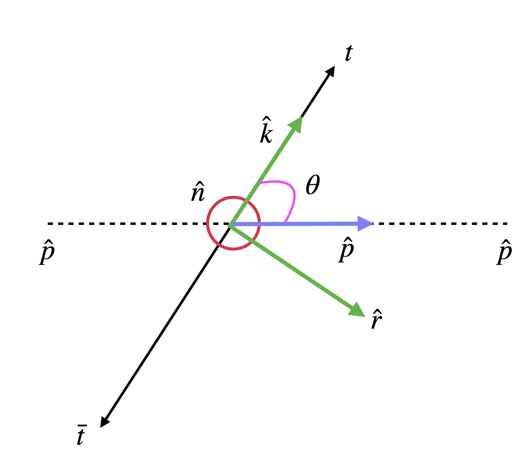
For the explicit matrix representation, we quantize both spins along $\hat{k}$ and order the states as

$\displaystyle|1\rangle=|+,-\rangle,\,\,|2\rangle=|+,+\rangle,\,\,|3\rangle=|-,-\rangle,\,\,|4\rangle=|-,+\rangle,$

(23)

where the entries label top and antitop helicity. Because the antitop moves opposite to $\hat{k}$, its helicity sign is opposite to its spin projection on the common $\hat{k}$ axis.

We use four complementary functions of $\rho$. The simplest is the purity,

$$\Gamma={\rm Tr}(\rho^{2}),$$

(24)

which ranges from $1/4$ for the maximally mixed two-qubit state to unity for a pure state. In the polarized analysis it indicates whether changing the initial helicity mixture merely changes the yield or also changes how coherently the final spin states are populated.

Following Refs. [36, 38, 39, 37, 86], we construct four entanglement markers from the three diagonal spin correlations:

	$\displaystyle\mathcal{D}^{(1)}$	$\displaystyle=$	$\displaystyle\frac{1}{3}\big(C_{kk}+C_{rr}+C_{nn}\big),$		(25)
	$\displaystyle\mathcal{D}^{(k)}$	$\displaystyle=$	$\displaystyle\frac{1}{3}\big(C_{kk}-C_{rr}-C_{nn}\big),$		(26)
	$\displaystyle\mathcal{D}^{(r)}$	$\displaystyle=$	$\displaystyle\frac{1}{3}\big(-C_{kk}+C_{rr}-C_{nn}\big),$		(27)
	$\displaystyle\mathcal{D}^{(n)}$	$\displaystyle=$	$\displaystyle\frac{1}{3}\big(-C_{kk}-C_{rr}+C_{nn}\big),$		(28)

and retain their minimum $\mathcal{D}_{\min}=\min_{a}\mathcal{D}^{(a)}$. A convenient sufficient criterion for entanglement is [97, 77]

$$\mathcal{D}_{\min}<-\frac{1}{3},$$

(29)

Failure to cross this boundary is inconclusive because off-diagonal correlations and one-particle polarizations do not enter this criterion. This experimentally robust construction has played a central role in top-entanglement measurements at the LHC [6, 75]. For an exact two-qubit entanglement measure we also calculate concurrence. Introduce the spin-flipped density matrix [76, 106]

$$\widetilde{\rho}=(\sigma_{2}\otimes\sigma_{2})\rho^{*}(\sigma_{2}\otimes\sigma_{2}),$$

(30)

and the positive matrix

$$\mathcal{R}_{\rho}=\sqrt{\sqrt{\rho}\,\widetilde{\rho}\,\sqrt{\rho}}.$$

(31)

If its eigenvalues are ordered as $\lambda_{1}\geq\lambda_{2}\geq\lambda_{3}\geq\lambda_{4}\geq 0$, then

$$C(\rho)=\max\{0,\lambda_{1}-\lambda_{2}-\lambda_{3}-\lambda_{4}\}.$$

(32)

Thus $C=0$ characterizes separable two-qubit states and $C=1$ a maximally entangled state. The associated entanglement of formation is [106]

$$E(\rho)=h\!\left(\frac{1+\sqrt{1-C(\rho)^{2}}}{2}\right),\text{ with }h(x)=-x\log_{2}x-(1-x)\log_{2}(1-x).$$

(33)

When top and antitop polarizations vanish ($\mathcal{B}_{1}=\mathcal{B}_{2}=0$) and $\mathcal{C}$ is diagonal, $\mathcal{D}_{\min}$ and concurrence are related by

$$C=\frac{1}{2}\max\{0,-1-3\mathcal{D}_{\min}\}.$$

(34)

Outside that restricted class of states, concurrence is evaluated from the full density matrix rather than inferred from $\mathcal{D}_{\min}$. Finally, we test whether the correlations are incompatible with a local hidden-variable description. For spin measurements along unit vectors $\hat{a}$ and $\hat{b}$, define

$$E(\hat{a},\hat{b})=\operatorname{Tr}\!\left[\rho(\hat{a}\cdot\boldsymbol{\sigma})\otimes(\hat{b}\cdot\boldsymbol{\sigma})\right]=\hat{a}^{T}\mathcal{C}\hat{b}.$$

(35)

The CHSH combination built from two settings on each side obeys

$$|E(\hat{a}_{1},\hat{b}_{1})-E(\hat{a}_{1},\hat{b}_{2})+E(\hat{a}_{2},\hat{b}_{1})+E(\hat{a}_{2},\hat{b}_{2})|\leq 2$$

(36)

in any local hidden-variable theory [31, 51, 66, 32]. Optimization over the four directions can be done algebraically. If $e_{1}\geq e_{2}\geq e_{3}$ are the eigenvalues of $\mathcal{C}^{T}\mathcal{C}$, the largest attainable value is [78, 79, 46]

$$\mathcal{B}_{\rm CHSH}\equiv B_{\max}=2\sqrt{e_{1}+e_{2}}.$$

(37)

We denote this Bell parameter by $\mathcal{B}_{\rm CHSH}$. Bell-inequality violation occurs for $\mathcal{B}_{\rm CHSH}>2$, while quantum mechanics limits it to $2\sqrt{2}$ [50]. Unlike concurrence, this quantity diagnoses Bell nonlocality rather than entanglement alone. Both can be obtained after reconstructing the spin density matrix from top-decay angular distributions [18, 16, 101, 63].

Numerically, we construct $\mathcal{R}$ from the SM and $U(1)$ helicity amplitudes, normalize it according to Eq. (6), and apply Eqs. (21) and (28) directly. Concurrence is always computed from the full $4\times 4$ matrix, while the maximal CHSH parameter is obtained from the two largest eigenvalues of $\mathcal{C}^{T}\mathcal{C}$. As an independent validation, we compared our analytically constructed $t\bar{t}$ spin-density matrices and the resulting $\mathcal{D}_{\min}$, concurrence, and $\mathcal{B}_{\rm CHSH}$ values with event-by-event results from the automated MadGraph density-matrix implementation of Ref. [61]. After accounting for the helicity-state phase convention, we find numerical agreement for both the density-matrix elements and the derived quantum observables.¹¹1To perform the validation we used the numerical code of the general U(1) model [53] from FeynRules..

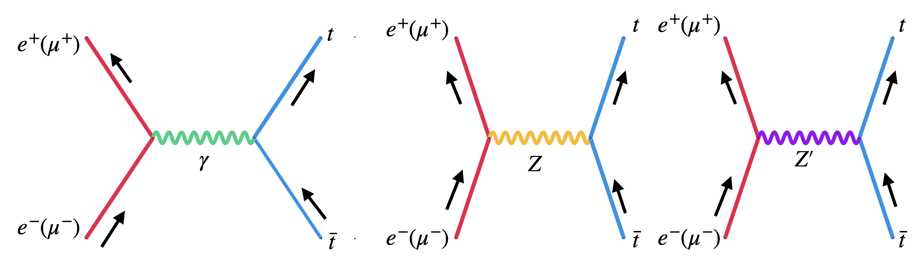
We work in the center-of-mass (CM) frame with massless incoming leptons and an outgoing $t\bar{t}$ pair whose constituents have mass $m_{t}$. The four-momenta are

$\displaystyle p_{1}^{\mu}=\frac{\sqrt{s}}{2}(1,0,0,1),\qquad p_{2}^{\mu}=\frac{\sqrt{s}}{2}(1,0,0,-1),$

(38)

with the lepton (antilepton) along $+z$ ($-z$). Choosing the $xz$-plane as the scattering plane, the final-state momenta are

$\displaystyle k_{1}^{\mu}$

$\displaystyle=\frac{\sqrt{s}}{2}\left(1,\beta\sin\theta,0,\beta\cos\theta\right),\qquad k_{2}^{\mu}=\frac{\sqrt{s}}{2}\left(1,-\beta\sin\theta,0,-\beta\cos\theta\right),$

(39)

with $\beta=\sqrt{1-4m_{t}^{2}/s}$ the top velocity and $\theta$ the scattering angle of $t$ relative to the beam axis. The orthonormal spin-correlation basis is

$\displaystyle\hat{k}=\frac{\mathbf{k}_{1}}{|\mathbf{k}_{1}|},\,\,\,\,\,\hat{p}=\frac{\mathbf{p}_{1}}{|\mathbf{p}_{1}|},\,\,\,\,\,\hat{r}=\frac{\hat{p}-\hat{k}\cos\theta}{\sin\theta},\,\,\,\,\,\hat{n}=\frac{\hat{p}\times\hat{k}}{\sin\theta}.$

(40)

This basis is used for the spin-correlation matrix $C_{ij}$ with $i,j\in\{r,n,k\}$. We use the chiral representation of the gamma matrices,

$\displaystyle\gamma^{0}=\begin{pmatrix}0&\mathbf{I}_{2\times 2}\\ \mathbf{I}_{2\times 2}&0\end{pmatrix},\;\gamma^{i}=\begin{pmatrix}0&-\sigma^{i}\\ \sigma^{i}&0\end{pmatrix},\gamma^{5}=\begin{pmatrix}-\mathbf{I}_{2\times 2}&0\\ 0&\mathbf{I}_{2\times 2}\end{pmatrix},\;P_{L,R}=\frac{1\mp\gamma^{5}}{2},$

(41)

and $\bar{\psi}=\psi^{\dagger}\gamma^{0}$. For a unit three-vector $\hat{p}$ with polar and azimuthal angles $(\theta,\phi)$, the two-component helicity spinors are

$$\chi(\hat{p})=\begin{pmatrix}\cos\frac{\theta}{2}\\[2.0pt] e^{i\phi}\sin\frac{\theta}{2}\end{pmatrix},\qquad\xi(\hat{p})=\begin{pmatrix}-e^{-i\phi}\sin\frac{\theta}{2}\\[2.0pt] \cos\frac{\theta}{2}\end{pmatrix}$$

(42)

obeying $(\boldsymbol{\sigma}\cdot\hat{p})\chi(\hat{p})=+\chi(\hat{p})$ and $(\boldsymbol{\sigma}\cdot\hat{p})\xi(\hat{p})=-\xi(\hat{p})$, respectively. For a fermion with $p^{\mu}=(E,\mathbf{p})$ and $p=|\mathbf{p}|$, we use the HELAS spinor convention [94]

$\displaystyle u(p,+)=\begin{pmatrix}\sqrt{E-p}\,\chi(\hat{p})\\ \sqrt{E+p}\,\chi(\hat{p})\end{pmatrix},u(p,-)=\begin{pmatrix}\sqrt{E+p}\,\xi(\hat{p})\\ \sqrt{E-p}\,\xi(\hat{p})\end{pmatrix},v(p,+)$

$\displaystyle=\begin{pmatrix}-\sqrt{E+p}\,\xi(\hat{p})\\ \sqrt{E-p}\,\xi(\hat{p})\end{pmatrix},v(p,-)=\begin{pmatrix}\sqrt{E-p}\,\chi(\hat{p})\\ -\sqrt{E+p}\,\chi(\hat{p})\end{pmatrix}.$

(43)

The azimuthal dependence is absorbed into the orthonormal basis $\{\hat{r},\hat{n},\hat{k}\}$, so the amplitudes depend only on the polar angle $\theta$. The full $t\bar{t}$ scattering amplitude is

$\displaystyle\mathcal{M}(\lambda_{\ell^{-}},\lambda_{\ell^{+}};\lambda_{t},\lambda_{\bar{t}})=\mathcal{M}_{\rm SM}(\lambda_{\ell^{-}},\lambda_{\ell^{+}};\lambda_{t},\lambda_{\bar{t}})+\mathcal{M}_{Z^{\prime}}(\lambda_{\ell^{-}},\lambda_{\ell^{+}};\lambda_{t},\lambda_{\bar{t}})$

(44)

where $\mathcal{M}_{\rm SM}$ contains photon and $Z$ exchange, and $\mathcal{M}_{Z^{\prime}}$ is the contribution from the additional $U(1)$ gauge boson. We denote helicities $-1/2$ and $+1/2$ by $-$ and $+$, respectively. For a gauge boson $V\in\{Z,Z^{\prime}\}$ with mass $M_{V}$ and total width $\Gamma_{V}$, we define the propagator denominator $\Delta_{V}=s-M_{V}^{2}+iM_{V}\Gamma_{V}$.

The SM helicity amplitudes from $s$-channel photon and $Z$ exchange are

	$\displaystyle\mathcal{M}_{\rm SM}(+,-;\pm,\pm)$	$\displaystyle=\sqrt{1-\beta^{2}}\,\sin\theta\left[e^{2}Q_{\ell}Q_{t}+\frac{s\,g_{Z}^{R\ell}}{2}\frac{g_{Z}^{Lt}+g_{Z}^{Rt}}{\Delta_{Z}}\right]$		(45)
	$\displaystyle\mathcal{M}_{\rm SM}(-,+;\pm,\pm)$	$\displaystyle=-\sqrt{1-\beta^{2}}\,\sin\theta\left[e^{2}Q_{\ell}Q_{t}+\frac{s\,g_{Z}^{L\ell}}{2}\frac{g_{Z}^{Lt}+g_{Z}^{Rt}}{\Delta_{Z}}\right]$		(46)
	$\displaystyle\mathcal{M}_{\rm SM}(+,-;\pm,\mp)$	$\displaystyle=(1\pm\cos\theta)\left[e^{2}Q_{\ell}Q_{t}+\frac{s\,g_{Z}^{R\ell}}{2}\frac{g_{Z}^{Lt}(1\mp\beta)+g_{Z}^{Rt}(1\pm\beta)}{\Delta_{Z}}\right]$		(47)
	$\displaystyle\mathcal{M}_{\rm SM}(-,+;\pm,\mp)$	$\displaystyle=(1\mp\cos\theta)\left[e^{2}Q_{\ell}Q_{t}+\frac{s\,g_{Z}^{L\ell}}{2}\frac{g_{Z}^{Lt}(1\mp\beta)+g_{Z}^{Rt}(1\pm\beta)}{\Delta_{Z}}\right]$		(48)

where $Q_{\ell}=-1$, $Q_{t}=2/3$, $M_{Z}=91.2$ GeV, and $\Gamma_{Z}=2.4955$ GeV [95]. The SM chiral couplings are

$\displaystyle g_{Z}^{L_{(\ell,t)}}=\frac{e(T_{3}^{(\ell,t)}-Q_{(\ell,t)}\sin^{2}\theta_{W})}{\cos\theta_{W}\sin\theta_{W}},\,\,\,g_{Z}^{R_{(\ell,t)}}$

$\displaystyle=-\frac{eQ_{(\ell,t)}\sin\theta_{W}}{\cos\theta_{W}}.$

(49)

For the numerical analysis we use $\sin^{2}\theta_{W}=0.23343$, together with $T_{3}^{\ell}=-1/2$ and $T_{3}^{t}=1/2$, consistently with Ref. [25]. The $s$-channel $Z^{\prime}$ helicity amplitudes in the $U(1)_{X}$ scenario are

	$\displaystyle\mathcal{M}_{Z^{\prime}}(+,-;\pm,\pm)$	$\displaystyle=-\frac{g_{X}^{2}\,m_{t}\sqrt{s}\,(x_{H}+1)(5x_{H}+4)\sin\theta}{6\,\Delta_{Z^{\prime}}}$		(50)
	$\displaystyle\mathcal{M}_{Z^{\prime}}(+,-;\pm,\mp)$	$\displaystyle=-\frac{g_{X}^{2}\sqrt{s}\,(x_{H}+1)\left[\sqrt{s}(5x_{H}+4)\pm 3\sqrt{s-4m_{t}^{2}}\,x_{H}\right](1\pm\cos\theta)}{12\,\Delta_{Z^{\prime}}}$		(51)
	$\displaystyle\mathcal{M}_{Z^{\prime}}(-,+;\pm,\pm)$	$\displaystyle=\frac{g_{X}^{2}\,m_{t}\sqrt{s}\,(x_{H}+2)(5x_{H}+4)\sin\theta}{12\,\Delta_{Z^{\prime}}}$		(52)
	$\displaystyle\mathcal{M}_{Z^{\prime}}(-,+;\pm,\mp)$	$\displaystyle=-\frac{g_{X}^{2}\sqrt{s}\,(x_{H}+2)\left[\sqrt{s}(5x_{H}+4)\pm 3\sqrt{s-4m_{t}^{2}}\,x_{H}\right](1\mp\cos\theta)}{24\,\Delta_{Z^{\prime}}}$		(53)

where $g_{X}$ is the general $U(1)_{X}$ coupling and $\Gamma_{Z^{\prime}}$ is the total decay width of $Z^{\prime}$. For $x_{H}=-2$ and $x_{\Phi}=1$, the general $U(1)_{X}$ model reduces to the $U(1)_{R}$ scenario. The same SM-fermion charge assignment is also obtained from the $U(1)_{xq-\tau_{R}^{3}}$ model by choosing $x=0$, while it has no equivalent realization in the $U(1)_{q+\tilde{x}u}$ framework. In this case the left-handed top quark has no direct coupling to the $Z^{\prime}$ boson. The choice $x_{H}=-0.5$ in the $U(1)_{X}$ model, equivalent to $x=1/4$ in $U(1)_{xq-\tau_{R}^{3}}$ and $\tilde{x}=0$ in $U(1)_{q+\tilde{x}u}$, gives a complementary chiral pattern in which the right-handed top quark has no direct $Z^{\prime}$ coupling. The vector-like B$-$L scenario is recovered by taking $x_{H}=0$ and $x_{\Phi}=1$ in the $U(1)_{X}$ model, $x=1/3$ in the $U(1)_{xq-\tau_{R}^{3}}$ model, and $\tilde{x}=1$ in the $U(1)_{q+\tilde{x}u}$ model. Finally, the charge assignment $x_{H}=2$ and $x_{\Phi}=1$ is equivalent to $x=2/3$ in the $U(1)_{xq-\tau_{R}^{3}}$ model and cannot be embedded in the $U(1)_{q+\tilde{x}u}$ framework. These representative charge assignments, summarized in Tab. 1, are used throughout our analysis to test how the $t\bar{t}$ spin-density matrix responds to different left- and right-handed $Z^{\prime}$ couplings.

We now discuss the numerical behavior of the quantum-information observables in the general $U(1)_{X}$ scenario. We first consider unpolarized initial beams, corresponding to Eq. (5), and then turn to polarized $e^{-}e^{+}$ beams using Eq. (7). The unpolarized results provide the baseline against which the polarization effects should be interpreted. Since the observables are constructed from the normalized spin density matrix, they are not simply proxies for the total rate; they probe how the helicity structure of $\gamma/Z/Z^{\prime}$ exchange reshapes the two-qubit spin state of the final $t\bar{t}$ pair.

Fig. 3 shows the sufficient entanglement marker $\mathcal{D}_{\min}$ over the $\sqrt{s}$–$\cos\theta$ plane up to $\sqrt{s}=20$ TeV. The white dashed lines mark representative lepton-collider energies, including the 10 TeV muon-collider benchmark. Regions with $\mathcal{D}_{\min}<-1/3$ correspond to spin-entangled $t\bar{t}$ states according to Eq. (29). The pattern depends sensitively on $x_{H}$ because left- and right-handed SM fermions carry different $U(1)_{X}$ charges. The angular dependence of $\mathcal{D}_{\min}$ therefore probes the chiral structure of the $Z^{\prime}$ interaction in addition to its mass and width.