Tensor-Network Finite Elements for Analytic Operator Equations

Let $\Omega$ denote the domain of the independent variable $\mathbf{q}$, $\mathcal{H}(\Omega)$ denote the corresponding admissible solution space, and $\mathcal{R}(\Omega)$ denote the residual space, whose elements quantify the extent to which a trial solution fails to satisfy the governing equation. We write a general OE over $\Omega$ as

$$\mathbf{L}[\mathbf{u}]=\mathbf{0}$$

(1)

where $\mathbf{L}:\mathcal{H}(\Omega)\rightarrow\mathcal{R}(\Omega)$, and $\mathbf{u}\in\mathcal{H}(\Omega)$. Then, consider a finite collection of scalar basis functions $b_{\beta}:\Omega\rightarrow\mathbb{F}$ where $\mathbb{F}$ indicates the scalar field. In FE representation, the solution can be approximated as

$$\mathbf{u}\approx\mathbf{c}^{\beta}b_{\beta}$$

(2)

where $\left[\mathbf{c}^{\beta}\right]$ is the coefficient tensor. The Galerkin weak formulation would requires

$$\int_{\Omega}b^{\ast}_{\beta}\mathbf{L}[\mathbf{u}]\,\mathrm{d}\mathbf{q}=\mathbf{0}$$

(3)

for every test function $b_{\beta}$ with decorator $\ast$ indicates conjugation. This reduces the continuous equation to a finite system of algebraic equations for the coefficient tensor.

We consider a general class of analytic OEs that admit a convergent Fréchet–Taylor expansion 5; 6; 46; 41; 16 of the form

$$\mathbf{L}[\mathbf{u}]=\sum_{\mathrm{i}=0}^{\infty}\dfrac{1}{\mathrm{i}!}\int_{\Omega^{\mathrm{i}}}\mathbf{k}_{\mathrm{i}}^{\left[\eta_{\mathrm{j}}\right]}\odot\bigotimes_{\mathrm{j}=1}^{\mathrm{i}}\partial_{\mathbf{q}_{\mathrm{j}}}^{\eta_{\mathrm{j}}}\mathbf{u}_{\mathrm{j}}\,\mathrm{d}\mathbf{q}_{\mathrm{j}}$$

(4)

where $\eta_{\mathrm{j}}\in\mathbb{N}_{0}$, $\mathbf{u}_{\mathrm{j}}=\mathbf{u}(\mathbf{q}_{\mathrm{j}})$, and $\mathbf{k}_{\mathrm{i}}^{\left[\eta_{\mathrm{j}}\right]}$ is an $\mathrm{i}$-linear interaction kernel with proper contraction to each $\partial_{\mathbf{q}_{\mathrm{j}}}^{\eta_{\mathrm{j}}}\mathbf{u}_{\mathrm{j}}$ as shown in Fig. 1.

If we further define

$$\mathbf{f}_{\mathrm{i},\left[\beta_{\mathrm{j}}\right]}=\dfrac{1}{\mathrm{i}!}\int_{\Omega^{\mathrm{i}}}\mathbf{k}_{\mathrm{i}}^{\left[\eta_{\mathrm{j}}\right]}\odot\bigotimes_{\mathrm{j}=1}^{\mathrm{i}}\partial_{\mathbf{q}_{\mathrm{j}}}^{\eta_{\mathrm{j}}}b_{\beta_{\mathrm{j}}}\,\mathrm{d}\mathbf{q}_{\mathrm{j}}$$

(5)

where $b_{\beta_{\mathrm{j}}}=b_{\beta_{\mathrm{j}}}(\mathbf{q}_{\mathrm{j}})$, the weak formulation can be written, for all $\beta$, as

$$\sum_{\mathrm{i}=0}^{\infty}\mathbf{g}_{\mathrm{i},\beta,\left[\beta_{\mathrm{j}}\right]}\odot\bigotimes_{\mathrm{j}=1}^{\mathrm{i}}\mathbf{c}^{\beta_{\mathrm{j}}}=\mathbf{0}$$

(6)

where the discretized operator tensor is defined as

$$\mathbf{g}_{\mathrm{i},\beta,\left[\beta_{\mathrm{j}}\right]}=\int_{\Omega}b^{\ast}_{\beta}\mathbf{f}_{\mathrm{i},\left[\beta_{\mathrm{j}}\right]}\,\mathrm{d}\mathbf{q}\,.$$

(7)

Suppose that $\Omega$ is partitioned into $N$ finite elements $\Omega_{\mathrm{n}}$, where $\mathrm{n}\in\{1,\ldots,N\}$, each with local basis functions $b_{\mathrm{n},\beta_{\mathrm{n}}}$ which are non-zero only in $\Omega_{\mathrm{n}}$, and elements can have different numbers of basis functions. For cleanliness, we will slightly abuse our notation by acting as if all elements contain the same number of basis functions. With this assumption, we can substitute $\mathrm{n}$ with a tensor index $\nu$, and we can replace Eq. 2 with

$$\mathbf{u}\approx\mathbf{c}^{\nu\beta}b_{\nu\beta}\,.$$

(8)

We can cascade this to the case for analytic OEs, and get the replacement for Eq. 6 as

$$\sum_{\mathrm{i}}\mathbf{g}_{\mathrm{i},\nu\beta,\left[\nu_{\mathrm{j}}\beta_{\mathrm{j}}\right]}\odot\bigotimes_{\mathrm{j}=1}^{\mathrm{i}}\mathbf{c}^{\nu_{\mathrm{j}}\beta_{\mathrm{j}}}=\mathbf{0}$$

(9)

where $\mathbf{g}_{\mathrm{i},\nu\beta,\left[\nu_{\mathrm{j}}\beta_{\mathrm{j}}\right]}$ can be obtain from simple substitution of basis function indexings.

The local approximation space on element $\mathrm{n}$ is the span of all local basis functions of that element. For normal FEM, the overall approximation Hilbert space $\Phi\subset\mathcal{H}(\Omega)$ is the direct sum of the local approximation spaces:

$$\Phi=\bigoplus_{\mathrm{n}=1}^{N}\Phi_{\mathrm{n}}$$

(10)

where

$$\Phi_{\mathrm{n}}=\text{Span}\left(\left\{b_{\mathrm{n},\beta_{\mathrm{n}}}\mid\beta_{\mathrm{n}}\in\{1,\ldots,B_{\mathrm{n}}\}\right\}\right)$$

(11)

and $B_{\mathrm{n}}$ is the number of basis functions in element $\mathrm{n}$. To build a TP representation, we use bra-ket notation from quantum mechanics, replacing each basis element by

$$b_{\mathrm{n},\beta_{\mathrm{n}}}\mapsto\ket{b_{\mathrm{n},\beta_\mathrm{n}}}\in\Phi\,.$$

(12)

If we were only interested in linear PDEs, we could stop here. All such equations can (trivially) be projected down to matrix equations acting on elements of the approximation Hilbert space $\Phi$. We are, however, primarily interested in the case of nonlinear PDEs. As such we define the Fock space by

$$\Psi=\bigoplus_{\mathrm{i}=0}^{\infty}\Phi^{\otimes\mathrm{i}}\,.$$

(13)

This space has a choice of basis vectors of the form

$$\ket{\left[\mathrm{n}_\mathrm{j}\beta_{\mathrm{n}_\mathrm{j}}\right]}_{\mathrm{i}}=\ket{\mathrm{n}_1\beta_{\mathrm{n}_1},\ldots,\mathrm{n}_\mathrm{i}\beta_{\mathrm{n}_\mathrm{i}}}\in\Psi\,.$$

(14)

By itself, the Fock space is not identified directly with approximation space over the physical domain. It serves as a space for variational coefficients. To obtain physical solution, one must define a projection. For the purpose of solving OEs, we will choose the projection from our physical interpretation of states in $\Psi$ where each basis vector represents a sequence of basis functions involve in a correlation term, e.g., if $\mathbf{u}\approx\widetilde{\mathbf{c}}^{\nu\beta}b_{\nu\beta}$, we will replace the coefficient for the standard 2-element correlation, $\widetilde{\mathbf{c}}^{\nu_{1}\beta_{\nu_{1}}}\otimes\widetilde{\mathbf{c}}^{\nu_{2}\beta_{\nu_{2}}}$, with the coefficient $\mathbf{c}^{2,\nu_{1}\beta_{\nu_{1}},\nu_{2}\beta_{\nu_{2}}}$ of the basis vector $\ket{\nu_1\beta_{\nu_1},\nu_2\beta_{\nu_2}}$. Of course, any extra information of the system, e.g., symmetries of the kernels, can simplify the formal space.

With this interpretation, we can fully replace every term in Eq. 4 and get

$$\mathbf{L}[\mathbf{u}]=\sum_{\mathrm{i}=0}^{\infty}\mathbf{F}_{\mathrm{i},\left[\nu_{\mathrm{j}}\beta_{\nu_{\mathrm{j}}}\right]}\odot\mathbf{c}^{\mathrm{i},\left[\nu_{\mathrm{j}}\beta_{\nu_{\mathrm{j}}}\right]}=\mathbf{0}$$

(15)

as our OE, where

$$\ket{\mathbf{u}}=\sum_{\mathrm{i}=0}^{\infty}\mathbf{c}^{\mathrm{i},\left[\nu_{\mathrm{j}}\beta_{\nu_{\mathrm{j}}}\right]}\ket{\left[\nu_\mathrm{j}\beta_{\nu_\mathrm{j}}\right]}_{\mathrm{i}}$$

(16)

is the formal solution in $\Psi$ and

$$\mathbf{F}_{\mathrm{i},\left[\nu_{\mathrm{j}}\beta_{\nu_{\mathrm{j}}}\right]}=\dfrac{1}{\mathrm{i}!}\int_{\Omega^{\mathrm{i}}}\mathbf{k}_{\mathrm{i}}^{\left[\eta_{\mathrm{j}}\right]}\odot\bigotimes_{\mathrm{j}=1}^{\mathrm{i}}\partial_{\mathbf{q}_{\mathrm{j}}}^{\eta_{\mathrm{j}}}b_{\nu_{\mathrm{j}}\beta_{\nu_{\mathrm{j}}}}\,\mathrm{d}\mathbf{q}_{\mathrm{j}}\,.$$

(17)

Similarly, the weak formulation can be written as

$$\sum_{\mathrm{i}=0}^{\infty}\mathbf{G}_{\mathrm{i},\beta,\left[\nu_{\mathrm{j}}\beta_{\nu_{\mathrm{j}}}\right]}\odot\mathbf{c}^{\mathrm{i},\left[\nu_{\mathrm{j}}\beta_{\nu_{\mathrm{j}}}\right]}=\mathbf{0}$$

(18)

where

$$\mathbf{G}_{\mathrm{i},\beta,\left[\nu_{\mathrm{j}}\beta_{\nu_{\mathrm{j}}}\right]}=\int_{\Omega}b^{\ast}_{\beta}\mathbf{F}_{\mathrm{i},\left[\nu_{\mathrm{j}}\beta_{\nu_{\mathrm{j}}}\right]}\,\mathrm{d}\mathbf{q}\,.$$

(19)

However, this finite system of algebraic equations has many more coefficients than Eq. 9. Hence, extra conditions, which can take the form of regularization or full-blown equations, are required.

Due to the $\mathrm{i}$-linearity of $\mathbf{k}_{\mathrm{i}}^{\left[\eta_{\mathrm{j}}\right]}$, we have guage freedom to permute the pair indices $\left(\nu_{\mathrm{j}},\beta_{\nu_{\mathrm{j}}}\right)$ of $\mathbf{G}_{\mathrm{i},\beta,\left[\nu_{\mathrm{j}}\beta_{\nu_{\mathrm{j}}}\right]}$ and $\mathbf{c}^{\mathrm{i},\left[\nu_{\mathrm{j}}\beta_{\nu_{\mathrm{j}}}\right]}$. We chose to follow a canonical ordering such that for any $\mathrm{j}^{\prime}>\mathrm{j}$, $\nu_{\mathrm{j}^{\prime}}\geq\nu_{\mathrm{j}}$, i.e., in order of element labels. Furthermore, if $\nu_{\mathrm{j}^{\prime}}=\nu_{\mathrm{j}}$, $\eta_{\mathrm{j}^{\prime}}\geq\eta_{\mathrm{j}}$, i.e., in order of derivative order as well.

We can also tensorized the summation over $\mathrm{i}$ by introducing, for each element, empty basis function $b_{\nu 0}$ into the local approximation space basis set in Eq. 11. With this addition and let $J$ be the largest correlation order contribution of the analytic OE from any element, we can map each basis vector in $\Psi$ to a new representation such that each element is pre-allocated with $J$ slots and the basis orders that appear in the basis vector are filled in the slots of their corresponding elements in the same order, e.g., if $J=3$ and $N=4$, the basis vector $\ket{13,14,21,22,33}$ is mapped to

$$\ket{(3,4,0),(1,2,0),(3,0,0),(0,0,0)}\,,$$

i.e., 2 contributions from element 1, 2 contributions from element 2, 1 contribution from element 3, and no contribution from element 4. Hence, Eq. 18 can be replaced with

$$\mathbf{G}_{\beta,\left[\beta_{\nu\mathrm{j}}\right]}\odot\mathbf{c}^{\left[\beta_{\nu\mathrm{j}}\right]}=\mathbf{0}$$

(20)

with appropriate substitution of $\mathbf{G}_{\beta,\left[\beta_{\nu\mathrm{j}}\right]}$’s definition. The equation can be neatly represented in tensor network format as shown in Fig. 2.

Effectively, one can directly solve Eq. 20 and obtain the desired approximate solution. However, directly storing the full coefficient tensor $\mathbf{c}$ classically requires $O\left(B^{NJ}\right)$ coefficient blocks, where $B=\max\left(\{B_{\mathrm{n}}\}\right)$ which grows exponentially with the problem size. The full tensor-product space therefore cannot be introduced as a direct storage format, but as a formal correlated approximation space to be compressed by any TN ansatz.

The choice of TN ansatz is arbitrary in the perspective of our formalism, but, if one already has expectation for the solution to contain some correlation and/or entanglement behaviors, the network can be designed to support them. One crucial assumption is the locality of correlation: we expected the correlation to only appear between neighboring elements. Figure 3 illustrates representative TN ansatzes under different local correlation geometries.

Similar to Fig. 2, Fig. 3a is the generic tensor representation of $\mathbf{c}$. Figure 3b shows a matrix product state (MPS) which is appropriate for one-dimensional element orderings with nearest-neighbor correlations while Fig. 3c shows a projected entangled pair state (PEPS) structure adapted for two-dimensional grid-like element connectivity. Figure 3d illustrates a higher-order or hypergraph-type (HG) tensor network capable of representing multi-element correlations beyond pair-wise interactions.

The bond dimensions (ranges of bond indices $\sigma$’s) control the amount of inter-element correlation that can be represented. If the maximum bond dimension in the TN is $S$, and the maximum bond degree (including hyper-bond) in the TN is $M$, then the storage requirement is

$$O(NB^{J}S^{M})$$

(21)

instead of $O(B^{NJ})$. Therefore, as long as the bond degree and correlation order are capped by a constant, the TN ansatz defines a polynomial-size variational manifold inside the exponentially large correlated coefficient space.

Given any formal coefficient tensor $\mathbf{c}$, the residual from weak formulation can be defined as

$$\mathbf{h}_{\beta}(\mathbf{c})=\mathbf{G}_{\beta,\left[\beta_{\nu\mathrm{j}}\right]}\odot\mathbf{c}^{\left[\beta_{\nu\mathrm{j}}\right]}\,.$$

(22)

We determine the correlated coefficients by minimizing the weighted residual norm

$$J(\mathbf{c})=W^{\beta^{\prime}\beta}\left(\mathbf{h}^{\dagger}_{\beta^{\prime}}(\mathbf{c})\odot\mathbf{h}_{\beta}(\mathbf{c})\right)\,,$$

(23)

where $W^{\beta^{\prime}\beta}$ is a positive-definite metric on the residual space. The TN approximation is obtained by restricting $\mathbf{c}$ to a chosen TN ansatz variational manifold $\mathcal{T}_{\mathrm{TN}}$:

$$\mathbf{c}_{\mathrm{TN}}=\arg\min_{\mathbf{c}\in\mathcal{T}_{\mathrm{TN}}}J(\mathbf{c}).$$

(24)

Although this objective is quadratic and convex in the unrestricted correlated coefficient tensor $\mathbf{c}$, the TN parametrization makes the global optimization generally non-convex. However, when all tensors in TN except one are fixed, the residual becomes linear in the active tensor. Therefore, each single-site local update reduces the optimization to a convex weighted least-squares sub-problem which is part of the reason for the success of density matrix renormalization group (DMRG) algorithm for MPS ansatz.

A partial differential equation (PDE) can be written as

$$\mathbf{g}\left(\mathbf{q},\left[\partial^{\eta}_{\mathbf{q}}\mathbf{u}\right]\right)=\mathbf{0}\,.$$

(25)

If $\mathbf{g}$ is analytic, then it can be expanded as a convergent series

$$\mathbf{g}\left(\mathbf{q},\left[\partial^{\eta}_{\mathbf{q}}\mathbf{u}\right]\right)=\sum_{\mathrm{i}}\dfrac{1}{\mathrm{i}!}\mathbf{a}_{\mathrm{i}}^{\left[\eta_{\mathrm{j}}\right]}\odot\bigotimes_{\mathrm{j}=1}^{\mathrm{i}}\partial_{\mathbf{q}}^{\eta_{\mathrm{j}}}\mathbf{u}\,,$$

(26)

which is a special case of Eq. 4 when

$$\mathbf{k}_{\mathrm{i}}^{\left[\eta_{\mathrm{j}}\right]}=\mathbf{a}_{\mathrm{i}}^{\left[\eta_{\mathrm{j}}\right]}\bigotimes_{\mathrm{j}=1}^{\mathrm{i}}\delta(\mathbf{q}_{\mathrm{j}}-\mathbf{q})\,.$$

(27)

An initial-value problem (IVP) is simply a variation of PDE with time as one of the domain dimensions. Hence, it is of the form

$$\mathbf{g}\left(t,\mathbf{q},\left[\partial^{\eta}_{\mathbf{q}}\partial^{\zeta}_{t}\mathbf{u}\right]\right)=\mathbf{0}\,.$$

(28)

If $\mathbf{g}$ is analytic,

$$\mathbf{g}\left(t,\mathbf{q},\left[\partial^{\eta}_{\mathbf{q}}\partial^{\zeta}_{t}\mathbf{u}\right]\right)\\ =\sum_{\mathrm{i}}\dfrac{1}{\mathrm{i}!}\mathbf{a}_{\mathrm{i}}^{\left[\zeta_{\mathrm{k}}\right],\left[\eta_{\mathrm{j}}\right]}\odot\bigotimes_{\mathrm{j}=1}^{\mathrm{i}}\bigotimes_{\mathrm{k}=\mathrm{j}+1}^{\mathrm{i}}\partial_{\mathbf{q}}^{\eta_{\mathrm{j}}}\partial_{t}^{\zeta_{\mathrm{k}}}\mathbf{u}\,.$$

(29)

For IVP, given $\mathbf{u}^{\prime}$ and some of its time derivatives at time $t$, the problem is to determine $\mathbf{u}$ and those time derivatives at $t+\Delta t$. There are many schemes one can use with varying degree of convergence criteria and computational costs. We will use a simple implicit Euler’s scheme as an example that replaces the analytic form of the IVP with

$$\mathbf{0}=\sum_{\mathrm{i}}\dfrac{1}{\mathrm{i}!}\mathbf{a}_{\mathrm{i}}^{\left[\zeta_{\mathrm{k}}\right],\left[\eta_{\mathrm{j}}\right]}\odot\bigotimes_{\mathrm{j}=1}^{\mathrm{i}}\bigotimes_{\mathrm{k}=\mathrm{j}+1}^{\mathrm{i}}\\ \partial_{\mathbf{q}}^{\eta_{\mathrm{j}}}\begin{cases}\dfrac{1}{\Delta t}\left(\partial_{t}^{\zeta_{\mathrm{k}}-1}\mathbf{u}-\partial_{t}^{\zeta_{\mathrm{k}}-1}\mathbf{u}^{\prime}\right),&\zeta_{\mathrm{k}}\neq 0\\ \mathbf{u},&\zeta_{\mathrm{k}}=0\end{cases}\,.$$

(30)

With some term arrangement, the equation can be written as a PDE on $\mathbf{v}=\left[\partial_{t}^{\zeta}\mathbf{u}\right]$, a special case of Eq. 4.

An integro-differential equation (IDE) is a generalization of PDE to include non-local interaction mostly in the form of integration kernel as

$$\mathbf{g}\left(\mathbf{q},\left[\partial^{\eta}_{\mathbf{q}}\mathbf{u}\right],\left[\int_{\Omega^{\mathrm{i}}}\mathbf{a}_{\mathrm{i}}\left(\mathbf{q},\left[\mathbf{q}_{\mathrm{j}}\right],\left[\partial^{\eta}_{\mathbf{q}_{\mathrm{j}}}\mathbf{u}_{\mathrm{j}}\right]\right)\,\prod_{\mathrm{j}=1}^{\mathrm{i}}\mathrm{d}\mathbf{q}_{\mathrm{j}}\right]\right)=\mathbf{0}\,.$$

(31)

If $\mathbf{g}$, and all $\mathbf{a}_{\mathrm{i}}$’s are analytic, then it can be expanded as a special case of Eq. 4 with multi-linear interaction kernel containing some Dirac delta functions for the parts that are not integrations in the IDE.

A memory-delay equation (MDE) is an IDE with non-local interaction in temporal dimension, i.e.,

$$\mathbf{0}=\mathbf{g}\Biggl(t,\mathbf{q},\left[\partial^{\eta}_{\mathbf{q}}\partial^{\zeta}_{t}\mathbf{u}\right],\\ \left.\left[\int_{\tau^{\mathrm{i}}}\mathbf{a}_{\mathrm{i}}\left(t,\left[t_{\mathrm{j}}\right],\mathbf{q},\left[\partial^{\eta}_{\mathbf{q}}\partial^{\zeta}_{t_{\mathrm{j}}}\mathbf{u}_{\mathrm{j}}\right]\right)\,\prod_{\mathrm{j}=1}^{\mathrm{i}}\mathrm{d}t_{\mathrm{j}}\right]\right)\,.$$

(32)

Similar to the IDE, if $\mathbf{g}$, and all $\mathbf{a}_{\mathrm{i}}$’s are analytic, then it can be expanded as a special case of Eq. 4.

As a continuation from Section V.2, the ending note of that sub-section implies that we only need to consider the IVPs with only first order time derivatives. Also, instead of $\mathbf{u}^{\prime}$ and $\mathbf{u}$, we will use $\mathbf{u}^{(\mathrm{t}-1)}$ and $\mathbf{u}^{(\mathrm{t})}$ notations where labels in parentheses indicate time step. Hence, for 1D, we are ultimately solving for $\mathbf{u}^{(\mathrm{t})}$ in

$$0=\sum_{\mathrm{i}}\dfrac{1}{\mathrm{i}!}a_{\mathrm{i}}^{\left[\zeta_{\mathrm{k}}\right],\left[\eta_{\mathrm{j}}\right]}\prod_{\mathrm{j}=1}^{\mathrm{i}}\prod_{\mathrm{k}=\mathrm{j}+1}^{\mathrm{i}}\\ \partial_{q}^{\eta_{\mathrm{j}}}\begin{cases}\dfrac{1}{\Delta t}\left(u^{(\mathrm{t})}-u^{(\mathrm{t}-1)}\right),&\zeta_{\mathrm{k}}=1\\ u^{(\mathrm{t})},&\zeta_{\mathrm{k}}=0\end{cases}\,.$$

(33)

which is a PDE but not in the same format as Eq. 26: the existence of $u^{(\mathrm{t}-1)}$ which can be treated as part of another term with lower correlation order of $u^{(\mathrm{t})}$.

It is straight forward to simply use the weak formalism directly on the equation, but it means that we need to calculate $\mathbf{G}$ from scratch at every time step since $u^{(\mathrm{t}-1)}$ got updated. Instead, we can leverage the deterministic structure of the IVP to pre-compute some parts. Different classes of OEs will be different but for IVE and, to extension, PDE the spatial derivatives and multiplications can be pre-formuated and approximated into concise weak forms.

As spatial derivatives and multiplications are local operators, with well-distributed basis function, any of their actions on $\Phi_{\mathrm{n}}$ can be approximated with a member of $\Phi_{\mathrm{n}}$. In other words, we can approximate the spatial derivatives and multiplications with some tensor contractions.

Consider an arbitrary spatial derivative of a basis function $b_{\mathrm{n},\beta}$ which can be approximated as

$$\partial_{\mathbf{q}}b_{\mathrm{n},\beta}\approx\mathbf{m}^{\beta^{\prime\prime}}b_{\mathrm{n},\beta^{\prime\prime}}\,,$$

(34)

which, by the weak formulation, gives

$$\int_{\Omega}b^{\ast}_{\mathrm{n},\beta^{\prime}}\partial_{\mathbf{q}}b_{\mathrm{n},\beta}\,\mathrm{d}q\approx\mathbf{m}^{\beta^{\prime\prime}}\int_{\Omega}b^{\ast}_{\mathrm{n},\beta^{\prime}}b_{\mathrm{n},\beta^{\prime\prime}}\,\mathrm{d}q\,.$$

(35)

We then define

	$\displaystyle\mathbf{P}_{\mathrm{n},\beta^{\prime}\beta}$	$\displaystyle=\int_{\Omega}b^{\ast}_{\mathrm{n},\beta^{\prime}}\partial_{\mathbf{q}}b_{\mathrm{n},\beta}\,\mathrm{d}q\,,$		(36)
	$\displaystyle Q_{\mathrm{n},\beta^{\prime}\beta^{\prime\prime}}$	$\displaystyle=\int_{\Omega}b^{\ast}_{\mathrm{n},\beta^{\prime}}b_{\mathrm{n},\beta^{\prime\prime}}\,\mathrm{d}q\,,$		(37)

which can be pre-computed given the basis functions. If $Q^{-1}_{\mathrm{n},\beta^{\prime\prime}\beta^{\prime}}$ is the matrix inverse of $Q_{\mathrm{n},\beta^{\prime}\beta^{\prime\prime}}$. Then, $\partial_{\mathbf{q}}$ on the element $\mathrm{n}$ can be approximated with

$$\mathbf{D}_{\mathrm{n},\beta^{\prime\prime}\beta}\approx Q^{-1}_{\mathrm{n},\beta^{\prime\prime}\beta^{\prime}}\mathbf{P}_{\mathrm{n},\beta^{\prime}\beta}\,.$$

(38)

We can also visualize it in the tensor circuit form as shown in Fig. 4a. Note that the label $\mathrm{n}$ is needed since each element has different sets of besis functions. Also, the index $q$ of the derivative tensor indicate the axis of differentiation.

Similarly, consider an arbitrary spatial multiplication of a pair of basis functions $b_{\mathrm{n},\beta_{1}}$ and $b_{\mathrm{n},\beta_{2}}$ which can be approximated as

$$b_{\mathrm{n},\beta_{1}}b_{\mathrm{n},\beta_{2}}\approx m^{\beta^{\prime\prime}}b_{\mathrm{n},\beta^{\prime\prime}}\,.$$

(39)

If we define,

	$\displaystyle P^{\prime}_{\mathrm{n},\beta^{\prime}\beta_{1}\beta_{2}}$	$\displaystyle=\int_{\Omega}b^{\ast}_{\mathrm{n}\,\beta^{\prime}}b_{\mathrm{n},\beta_{1}}b_{\mathrm{n},\beta_{2}}\,\mathrm{d}q\,,$		(40)
	$\displaystyle Q^{\prime}_{\mathrm{n},\beta^{\prime}\beta^{\prime\prime}}$	$\displaystyle=\int_{\Omega}b^{\ast}_{\mathrm{n},\beta^{\prime}}b_{\mathrm{n},\beta^{\prime\prime}}\,\mathrm{d}q\,,$		(41)

then, any multiplication in this elemental basis can be approximated with tensor product reduction

$$R_{\mathrm{n},\beta^{\prime\prime}\beta_{1}\beta_{2}}=Q^{\prime-1}_{\mathrm{n},\beta^{\prime\prime}\beta^{\prime}}P^{\prime}_{\mathrm{n},\beta^{\prime}\beta_{1}\beta_{2}}\,,$$

(42)

as depicted in Fig. 4b.

With these components, we can construct other more complicated IVP operators, e.g., second derivative, dot product, cross product, divergence, curl, and Laplacian, as illustrated in Fig. 5. Of course, directly applying the weak formalism for each operator would give a better approximation at the cost of additional overhead calculations per time step.

We’ll apply the procedure of converting IVPs to TN with the following non-linear diffusion equations

$$\partial_{t}u=u^{\mathrm{p}}\partial^{2}_{x}u$$

(43)

with $u=u(t,x)$, $\mathrm{p}\in\{0,1,2\}$, $\Omega=[0,1]$, $u(0,x)$ is a modified Gaussian centered at $x=0.5$ with $\partial_{x}u(t,0)=\partial_{x}u(t,1)=0$, i.e., close boundaries. We can rewrite the IVP in our format as

$$0=u^{(\mathrm{t})\mathrm{p}}\partial^{2}_{x}u^{(\mathrm{t})}-\dfrac{1}{\Delta t}(u^{(\mathrm{t})}-u^{(\mathrm{t}-1)})\,.$$

(44)

The corresponding tensor circuit of this IVP is as shown in Fig. 6.

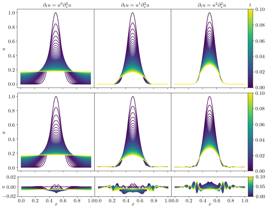
Then, we solve the non-linear diffusion IVP for each exponent $\mathrm{p}$ using $N$ uniform finite elements on $\Omega$, each equipped with $B$ local Lagrange polynomial basis functions, and an MPS ansatz with bond dimension $S$ for the coefficient tensor. The time evolution is advanced using the implicit Euler scheme described with time step $\Delta t$. At each time step, the DMRG sweep algorithm minimizes the weighted residual $J(\mathbf{c})$ over the MPS variational manifold $\mathcal{T}_{\mathrm{MPS}}$.

To ensure the continuity and smoothness of the results, we also add an additional circuit to measure the residual of multiple derivative orders at each boundary between elements as well as the residual of Neumann boundary conditions at the outer edges of the domain to environment. As these continuities only involve at most 2 adjacent elements, the circuit blocks either only connect adjacent tensor index branches (element boundaries) or only connect to one branch (domain edges).

Figure 7 summarize the time-evolution results across all three cases for explicit Runge-Kutta IVP simulation (top row) and TN variational (middle row) method. For $\mathrm{p}=0$ (left column), the equation reduces to the standard diffusion equation $\partial_{t}u=\partial_{x}^{2}u$, which admits a smooth, rapidly decaying solution. For $\mathrm{p}=1$ (middle column), the non-linear coupling $u\partial_{x}^{2}u$ introduces amplitude-dependent diffusion, slowing the spread of $u$ in regions of low amplitude. Finally, for $\mathrm{p}=2$ (right column), the stronger non-linearity further suppresses diffusion and produces sharper features. In all cases, the TN variational method with $N=10$, $B=4$, $S=1$ produce a reliable results with the difference of less than two percent of the original amplitude of the modified Gaussian as shown in the bottom row of Fig. 7. We also see that the Neumann boundary conditions at both ends of the domain as well as the continuity and smoothness of the results are also respected to within numerical precision confirming that the weak formulation correctly encodes the boundary constraints.

To assess the convergence properties of the TN solver, we study the behavior of the solution error as functions of Lagrange polynomial basis order $B$, and the number of finite elements $N$ at different time step size $\Delta t$. Since both $B$ and $N$ are, in some way, representation of spatial resolution, we should expect the behavior of the trend to be similar to standard finite difference method which exhibit the stability condition where the convergence cannot be improved purely by increasing spatial resolution while the temporal resolution is fixed. This is clearly shown in Fig. 8.

Together, these results demonstrate that the TN framework introduced in this paper can produce accurate, converged solutions to non-linear IVPs with the computational scaling controlled by the bond dimension rather than the full exponential size of the coefficient space. While the examples here are restricted to 1D MPS/DMRG for clarity, the formalism is directly extensible to higher-dimensional problems via PEPS or tree tensor network ansatzes.

References

- [1] (2008) Entanglement renormalization and topological order. Phys. Rev. Lett. 100, pp. 070404. External Links: Document, Link Cited by: §I.
- [2] (2023) Quantum algorithm for the linear vlasov equation with collisions. Phys. Rev. A 107, pp. 062412. External Links: Document, Link Cited by: §I.
- [3] (2009) Theoretical numerical analysis: a functional analysis framework. 3 edition, Texts in Applied Mathematics, Vol. 39, Springer, New York. Cited by: §I.
- [4] (2016) Tensor networks and hierarchical tensors for the solution of high-dimensional partial differential equations. Foundations of Computational Mathematics 16 (6), pp. 1423–1472. External Links: ISSN 1615-3383, Document, Link Cited by: §I.
- [5] (1984) Analytical foundations of Volterra series. IMA Journal of Mathematical Control and Information 1 (3), pp. 243–282. Cited by: §III.2.
- [6] (1985) Fading memory and the problem of approximating nonlinear operators with Volterra series. IEEE Transactions on Circuits and Systems 32 (11), pp. 1150–1161. Cited by: §III.2.
- [7] (2008) The mathematical theory of finite element methods. 3 edition, Texts in Applied Mathematics, Vol. 15, Springer, New York. Cited by: §I.
- [8] (2011) Functional analysis, sobolev spaces and partial differential equations. Universitext, Springer, New York. Cited by: §I.
- [9] (2009) Explicit tensor network representation for the ground states of string-net models. Physical Review B 79 (8), pp. 085119. External Links: Document, Link Cited by: §I.
- [10] (2013) Quantum algorithm and circuit design solving the poisson equation. New Journal of Physics 15 (1), pp. 013021. External Links: Document, Link Cited by: §I.
- [11] (2008) An introduction to the density matrix renormalization group ansatz in quantum chemistry. In Frontiers in quantum systems in chemistry and physics, pp. 49–65. Cited by: §I.
- [12] (2015) Spectral tensor networks for many-body localization. Phys. Rev. B 92, pp. 024201. External Links: Document, Link Cited by: §I.
- [13] (2002) The finite element method for elliptic problems. Classics in Applied Mathematics, Vol. 40, Society for Industrial and Applied Mathematics (SIAM), Philadelphia, PA. Note: Reprint of the 1978 North-Holland edition Cited by: §I.
- [14] (2016) Improved energy extrapolation with infinite projected entangled-pair states applied to the two-dimensional hubbard model. Phys. Rev. B 93, pp. 045116. External Links: Document, Link Cited by: §I.
- [15] (2019) Quantum algorithm for simulating the wave equation. Phys. Rev. A 99, pp. 012323. External Links: Document, Link Cited by: §I.
- [16] (1999) Complex analysis on infinite dimensional spaces. Springer Monographs in Mathematics, Springer, London. Cited by: §III.2.
- [17] (1980) A family of embedded runge-kutta formulae. Journal of Computational and Applied Mathematics 6 (1), pp. 19–26. External Links: ISSN 0377-0427, Document, Link Cited by: Figure 7.
- [18] (2015) Tensor network trial states for chiral topological phases in two dimensions and a no-go theorem in any dimension. Physical Review B 92 (20), pp. 205307. External Links: Document, Link Cited by: §I.
- [19] (1992) Finitely correlated states on quantum spin chains. Communications in Mathematical Physics 144 (3), pp. 443–490. External Links: ISSN 1432-0916, Document, Link Cited by: §I.
- [20] (2014) Tensor networks and quantum error correction. Phys. Rev. Lett. 113, pp. 030501. External Links: Document, Link Cited by: §I.
- [21] (2022) Language design as information renormalization. SN Computer Science 3 (2), pp. 140. External Links: ISSN 2661-8907, Document, Link Cited by: §I.
- [22] (2021) Quantum-inspired algorithms for multivariate analysis: from interpolation to partial differential equations. Quantum 5, pp. 431. External Links: Document, Link Cited by: §I.
- [23] (2022) A quantum-inspired approach to exploit turbulence structures. Nature Computational Science 2 (1), pp. 30–37. External Links: ISSN 2662-8457, Document, Link Cited by: §I.
- [24] (2009) Tensor-product representations for string-net condensed states. Physical Review B 79 (8), pp. 085118. External Links: Document, Link Cited by: §I.
- [25] (2013) Entanglement renormalization for quantum fields in real space. Physical Review Letters 110 (10), pp. 100402. External Links: Document, Link Cited by: §I.
- [26] (2018) Unsupervised generative modeling using matrix product states. Phys. Rev. X 8, pp. 031012. External Links: Document, Link Cited by: §I.
- [27] (2019) Towards quantum machine learning with tensor networks. Quantum Science and Technology 4 (2), pp. 024001. External Links: Document, Link Cited by: §I.
- [28] (2000) The finite element method: linear static and dynamic finite element analysis. Dover Publications, Mineola, NY. Note: Reprint of the 1987 Prentice-Hall edition Cited by: §I.
- [29] (2008) Density matrix renormalization group numerical study of the kagome antiferromagnet. Phys. Rev. Lett. 101, pp. 117203. External Links: Document, Link Cited by: §I.
- [30] (1991) Equivalence and solution of anisotropic spin-1 models and generalized t-j fermion models in one dimension. Journal of Physics A: Mathematical and General 24 (16), pp. L955. External Links: ISSN 0305-4470, Document, Link Cited by: §I.
- [31] (1993) Matrix product ground states for one-dimensional spin-1 quantum antiferromagnets. Europhysics Letters 24 (4), pp. 293. External Links: ISSN 0295-5075, Document, Link Cited by: §I.
- [32] (1972) Approximate solution of operator equations. Wolters-Noordhoff Publishing, Groningen. Cited by: §I.
- [33] (2016) Fermionic orbital optimization in tensor network states. Phys. Rev. Lett. 117, pp. 210402. External Links: Document, Link Cited by: §I.
- [34] (2021) Solving nonlinear differential equations with differentiable quantum circuits. Phys. Rev. A 103, pp. 052416. External Links: Document, Link Cited by: §I.
- [35] (2007) Finite difference methods for ordinary and partial differential equations: steady-state and time-dependent problems. Classics in Applied Mathematics, Society for Industrial and Applied Mathematics (SIAM), Philadelphia, PA. Cited by: §I.
- [36] (2019) Quantum entanglement in deep learning architectures. Physical Review Letters 122 (6), pp. 065301. External Links: Document, Link Cited by: §I.
- [37] (2019) Machine learning by unitary tensor network of hierarchical tree structure. New Journal of Physics 21 (7), pp. 073059. External Links: Document, Link Cited by: §I.
- [38] (2021) Variational quantum algorithm for the poisson equation. Phys. Rev. A 104, pp. 022418. External Links: Document, Link Cited by: §I.
- [39] (2018) Multigrid renormalization. Journal of Computational Physics 372, pp. 587–602. External Links: ISSN 0021-9991, Document, Link Cited by: §I.
- [40] (2008) Simulating quantum computation by contracting tensor networks. SIAM Journal on Computing 38 (3), pp. 963–981. External Links: Document, Link, https://doi.org/10.1137/050644756 Cited by: §I.
- [41] (1986) Complex analysis in Banach spaces: holomorphic functions and domains of holomorphy in finite and infinite dimensions. North-Holland Mathematics Studies, Vol. 120, North-Holland, Amsterdam. Cited by: §III.2.
- [42] (2014) A practical introduction to tensor networks: matrix product states and projected entangled pair states. Annals of Physics 349, pp. 117–158. External Links: Document Cited by: §I.
- [43] (2005) Exploiting quantum parallelism to simulate quantum random many-body systems. Phys. Rev. Lett. 95, pp. 140501. External Links: Document, Link Cited by: §I.
- [44] (2016) Spin- kagome quantum antiferromagnets in a field with tensor networks. Phys. Rev. B 93, pp. 060407. External Links: Document, Link Cited by: §I.
- [45] (2016) Efficient variational diagonalization of fully many-body localized hamiltonians. Phys. Rev. B 94, pp. 041116. External Links: Document, Link Cited by: §I.
- [46] (1980) The Volterra and Wiener theories of nonlinear systems. John Wiley & Sons, New York. Cited by: §III.2.
- [47] (2016) Supervised learning with tensor networks. In Advances in Neural Information Processing Systems, D. Lee, M. Sugiyama, U. Luxburg, I. Guyon, and R. Garnett (Eds.), Vol. 29, pp. . External Links: Link Cited by: §I.
- [48] (2004) Finite difference schemes and partial differential equations. 2 edition, Society for Industrial and Applied Mathematics (SIAM), Philadelphia, PA. Cited by: §I.
- [49] (2012) Entanglement renormalization and holography. Physical Review D 86 (6), pp. 065007. External Links: Document, Link Cited by: §I.
- [50] (2015) Tensor product methods and entanglement optimization for ab initio quantum chemistry. International Journal of Quantum Chemistry 115 (19), pp. 1342–1391. External Links: Document, Link Cited by: §I.
- [51] (1995) Numerical partial differential equations: finite difference methods. Texts in Applied Mathematics, Vol. 22, Springer, New York. Cited by: §I.
- [52] (2004) Renormalization algorithms for quantum-many body systems in two and higher dimensions. arXiv. External Links: cond-mat/0407066, Link Cited by: §I.
- [53] (2010) Continuous matrix product states for quantum fields. Physical Review Letters 104 (19), pp. 190405. External Links: Document, Link Cited by: §I.
- [54] (2007) Entanglement renormalization. Physical Review Letters 99 (22), pp. 220405. External Links: Document, Link Cited by: §I.
- [55] (1992) Density matrix formulation for quantum renormalization groups. Phys. Rev. Lett. 69, pp. 2863–2866. External Links: Document, Link Cited by: §I.
- [56] (1993) Density-matrix algorithms for quantum renormalization groups. Physical Review B 48 (14), pp. 10345–10356. External Links: Document, Link Cited by: §I.
- [57] (2022) Quantum-inspired method for solving the vlasov-poisson equations. Phys. Rev. E 106, pp. 035208. External Links: Document, Link Cited by: §I.
- [58] (2013) The finite element method: its basis and fundamentals. 7 edition, Butterworth-Heinemann (Elsevier), Oxford. Cited by: §I.