Q-SCM: A Quantum-Sequential Choice Model for Driver Mental State Evolution

Rulla Al-Haideri Affiliation: Laboratory of Innovations in Transportation (LiTrans), Toronto Metropolitan University Bilal Farooq Thanks: Corresponding author. Email: bilal.farooq@torontomu.ca Affiliation: Laboratory of Innovations in Transportation (LiTrans), Toronto Metropolitan University Karim Ismail Affiliation: Department of Civil and Environmental Engineering, Carleton University

Abstract

Driver behaviour in traffic interactions is shaped by evolving perception, exposure to perceptual cues, and the order in which risk related information is processed in the driver’s mind. Conventional latent class choice models can represent unobserved behavioural heterogeneity, however, class membership is commonly specified as a static or observation specific function of observed covariates. Although lagged variables or dynamic extensions can be added, these models do not usually provide an explicit and natural mechanism where cue history, cue processing order, and phase-like memory jointly shape the evolution of a driver’s latent mental state. We propose a Quantum-Sequential Choice Model (Q-SCM) for modelling driver mental state evolution in interactive traffic environments. The proposed framework retains the classical latent class choice structure, but replaces the conventional class membership formulation with a quantum cognitive state model. A unique feature of this model is that the quantum component is confined to the class membership layer, while the action choice layer remains a classical RUM. The driver’s latent state is represented as a two-state quantum system on the Bloch sphere including neutral and defensive states. Perceptual cues, including separation distance, closing time-to-collision (CTTC), and lane deviation induce sequential unitary rotations governed by Pauli matrices. This formulation allows the model to capture memory, phase effects, cue order dependence, and transitions between behavioural regimes that depend on prior cue history. To ensure well behaved state evolution, we introduce three control mechanisms: a monotonicity constraint that prevents pendulum-like overshoot, a geodesic safeguard mechanism that ensures convergence toward the defensive state under sustained threat exposure, and a relaxation step that allows recovery toward the neutral baseline when the threat weakens. The model is estimated using 85,754 observations from 9,610 drivers extracted from naturalistic trajectories. The empirical results show that defensive state formation is not governed only by the instantaneous values of traffic cues, but also by the accumulated cue history and the order in which cues are processed. In particular, state changing cues, represented by separation distance and CTTC, directly increase the defensive probability. The phase changing cue, represented by lane deviation, modifies how subsequent state changing cue are interpreted. These findings suggest that Q-SCM provides a behaviourally meaningful framework for representing memory, cue order effects, and evolving defensive appraisal in driver behaviour modelling.

¹¹footnotetext: Corresponding author. Email: bilal.farooq@torontomu.ca

1 Introduction

Latent class models are widely used in discrete choice modelling to capture unobserved behavioural heterogeneity. In these models, observed choices are assumed to emerge from a mixture of latent behavioural classes. The final choice probability is obtained by weighting class specific choice probabilities by the probability that the decision maker belongs to each class [9]. This structure is attractive for driver behaviour modelling because drivers may interpret the same traffic interaction differently. For example, the same surrounding traffic conditions may be perceived as routine by one driver but threatening to another driver. In many applications, latent class membership could be specified as a function of observed individual characteristics, contextual variables, or traffic interaction indicators [2]. This provides a flexible and interpretable way to explain heterogeneity across drivers or observations. However, driving is not only a response to contemporaneous conditions. It is a sequential cognitive process where previous cue exposure, cue processing order, and the accumulated internal state can influence how the next cue is interpreted. A driver who has just experienced a rapidly closing vehicle may not process the next separation distance in the same way as a driver who reached that same separation distance after a stable interaction. Therefore, the evolution of latent state membership is fundamental to modelling defensive driving behaviour.

In this paper, we model the driver’s observed manoeuvre choice at each trajectory sample. The proposed model assumes that this observed manoeuvre is influenced by an unobserved mental state, represented here as either neutral or defensive. The role of the quantum component is not to predict the manoeuvre directly. It is employed to generate the time varying probabilities of these latent states. These state probabilities are then passed to a classical choice layer, which obtains the probability of the observed manoeuvre. Classic latent class models can be extended to represent these effects. For example, lagged variables, interaction terms, hidden Markov structures or dynamic latent variables can be used to introduce memory, order dependence, and state transitions. Hence, the contribution of this paper is not based on the claim that classical latent class models are incapable of representing such behaviour. Instead, the motivation is that these effects often require additional variables, parameters, transition equations, or model specific assumptions. The quantum probability theory (QPT) provides a parsimonious and natural mathematical structure where memory, phase, and order dependence emerge directly from sequential state evolution [16, 4].

QPT has emerged in cognitive science as an alternative formalism to model human judgment and decision making under uncertainty [6, 17].The term “quantum” in this context does not imply that the brain is physically a quantum system. The quantum cognition uses the mathematical structure of QPT to describe cognitive phenomena that are difficult to represent parsimoniously using a single fixed classical probability space. These phenomena include, order effects [18, 22], interference and conjunction-disjunction violations [16], entanglement-like context dependence in concept combinations [1] and state change in evaluation [4]. In this framework, an individual’s cognitive state is represented by a state vector, and an evaluation changes that state. Then, the probability of a later judgment or action can depend on the sequence of prior evaluations. This distinction is important for driver behaviour. In classical probability theory (CPT), events are represented within a common sample space. The probabilities are updated according to classical rules. In QPT, cognitive evaluations can be incompatible [6]. Incompatibility means that evaluating one aspect of a situation can change the state from which another aspect is evaluated. This produces non-commutative updating, which means that processing cue $A$ followed by cue $B$ does not necessarily produce the same final state as processing cue $B$ followed by cue $A$ . Behaviourally, the order in which information is processed can affect the resulting judgment, even when the same information is available. This has been documented in attitude judgment surveys [21, 22] and in inference tasks [18].

In addition, quantum cognition introduces the concept of phase. In a classical probability model, the probability assigned to a latent state is usually sufficient to describe the state of belief relevant to that outcome. However, in QPT, a cognitive state includes both probability amplitudes and relative phase [16, 6]. The squared magnitudes of the amplitudes produce observable probabilities. The phase includes additional information about the cognitive context. In other words, two individuals can have the same observed probability of being in a given state but different phases. This can lead to different responses to the same subsequent cue. This feature is fundamental to the proposed model because it allows prior cue history to affect future state evolution even when the current defensive probability appears identical. These concepts are a useful foundation for modelling driver mental state evolution of individuals. Driving task involves continuous assessment, perception and sequential appraisal under time pressure. Drivers process multiple traffic cues before making an observable manoeuvre choice (i.e., action). These cues are not interpreted independently. Earlier cues may change the internal state from where later cues are evaluated. A traffic cue may directly increase the driver’s defensive appraisal. But another cue may not change the defensive probability immediately but may alter how subsequent cues are interpreted. This is the type of sequential and context dependent process that quantum cognition was appropriate to capture.

This paper proposes a Quantum-Sequential Choice Model (Q-SCM) for modelling driver mental state evolution in interactive traffic environments. The proposed framework retains the classical latent class choice structure. The class membership is reformulated using a quantum cognitive state model while the conditional choice layer remains classical. Once the probabilities of the latent states are obtained, the final action probability is computed as a weighted sum of class specific choice probabilities. The proposed contribution focuses on how class membership probabilities are generated. The Q-SCM represents class membership as an evolving cognitive state shaped by perceived sequential cue updates. An important feature of the proposed model is that the quantum mechanism is restricted to the class membership layer. The conditional choice layer remains a classical random utility model (RUM). This distinguishes Q-SCM from existing quantum choice models as is reviewed in Section 2. In those existing models the state vector represents the choice alternatives. The choice probabilities are obtained either directly from the Born rule or by adding a quantum interference term inside the choice equation. Thus, the RUM structure is either replaced or modified. In contrast, the quantum probabilities in Q-SCM never enter the choice equation directly. Instead, they only generate the latent class membership weights. This leaves the RUM choice layer intact and maintains the interpretability and welfare-analytic properties of standard discrete choice models.

The main objective of this paper is to develop and empirically demonstrate a parsimonious choice framework for modelling driver manoeuvre choice when the probability of being in a latent mental state evolves over time. Specifically, the paper aims to represent the driver’s neutral and defensive states as an evolving quantum cognitive state that is updated sequentially by perceptual traffic cues, while retaining a classical RUM for the observed manoeuvre choice. The contributions of this paper are fourfold. First, it proposes a new formulation for latent class membership where class probabilities are generated by a sequential quantum cognitive state model rather than a conventional class membership formulation. Second, it develops a two mental state representation of driver mental state evolution, where perceptual cues update the state through Bloch sphere rotations and the resulting state probabilities enter a classical latent class choice model. Third, unlike existing quantum choice models, which obtain choice probabilities from the Born rule or embed a quantum interference term inside the choice equation over the alternatives, the Q-SCM confines the quantum mechanism to the class membership layer and retains a fully classical RUM choice layer. Fourth, it demonstrates the proposed formulation using naturalistic trajectory data and compares it with a classical latent class benchmark that uses the same conditional choice layer.

The remainder of the paper is organized as follows. Section 2 reviews the relevant literature. Section 3 presents the proposed Q-SCM framework and explains how the quantum membership layer is combined with the classical manoeuvre choice layer. Section 4 applies the proposed framework to a publicly-available naturalistic trajectory dataset. Section 5 presents the estimation results and discusses the behavioural interpretation of the model. Section 6 concludes the paper.

2 Background

Hanckock et al. [11] developed choice models based on QPT. Their models represent the preferences of an individual using a belief state (i.e., state vector) as a unit vector in a complex Hilbert space. In their model, each alternative is set at an axis. The choice probabilities are obtained by squaring the projection of that vector onto each alternative (i.e., Born rule). They develop two versions of the model. The amplitude model captures the final belief state amplitudes as a function of attribute differences between alternatives. The Hamiltonian model evolves an initial belief state over time using the Schrödinger equation. The models also employ quantum rotations to capture context and order effects, such as changes in perspective when choosing the best alternative versus the worst alternative. However, these models are not RUMs as they replace the additive error and utility maximization structure with choice probabilities derived from probability amplitudes by the Born rule. As an extension to these quantum choice models, Hanckock et al. [10] further extend the quantum amplitude framework for moral choices. Those choices represent ones that are defined by a change of perspective by the decision maker using two mechanisms. The first one applies a quantum rotation based on the Pauli matrices to the state vector when a morally charged trade-off is present which affects the choice probabilities of the alternatives. The second assigns a separate complex phase to each attribute specific value function. This allows moral attributes such as deaths and injuries, to be processed differently from concrete attributes like time and cost.

Epping et al. [8] compared three models that capture how individuals make choices between two alternatives. They focused on jointly predicting which alternative is chosen and how long does the decision takes. Vitetta [20] proposed a quantum utility model (QUM) for route choice when individuals retain multiple possible routes before making a final decision during the trip. The model extends classical RUM probability by adding a quantum interference term that captures the coexistence of intermediate route preferences. When the pre-trip decision is unique, the interference term collapses and the QUM reduces to conventional RUM. But when multiple alternatives coexist, the model departs from the classical RUM formulation. Di Gangi and Vitetta [7] proposed QUARUM (Quantum Utility integrated with a Random Utility Model) for route choice. The model retains the classical RUM structure and adds a QUM-derived interference term at the route generation level to represent interactions among candidate routes during perception. After this perception stage, route choice is modelled using a RUM formulation where route overlap is accounted for by a covariance structure among alternatives. Lipovetsky [14] used probability amplitudes to model when individuals make choices when selecting among competing products. In their formulation, each alternative corresponds to one component of a state vector representing the decision maker’s preferences. Those components are complex probability amplitudes where the squared moduli produce the choice probabilities. Yu and Jayakrishnan [23] proposed a quantum model where the traveler’s mental state is represented as a state vector in a Hilbert space. The survey question and the real world decision were treated as two different measurements acting on that state. Each possible choice such as driving alone or taking a ride sharing service is represented as its own direction in this space. Then the probability of a choice is given by how closely the mental state vector aligns with that direction.

To the authors’ knowledge, there is no existing study that has formulated the quantum state vector as an evolving latent cognitive state which updates sequentially by perceptual traffic cues to generate class membership probabilities in a choice model. In the reviewed quantum choice models, the state vector generally represents preferences over choice alternatives, the basis axes correspond to those alternatives, and choice probabilities are obtained from the Born rule. Thus, the quantum component operates at the level of the alternatives rather than at the level of an internal driver state that carries memory of prior cues before an action is chosen.

Table 1 summarizes this distinction. Most reviewed quantum choice models replace the additive random utility and utility maximization structure with probabilities derived from quantum amplitudes. The main exceptions are the quantum utility models of Vitetta [20] and Di Gangi and Vitetta [7]. They retain a RUM component but augment the alternative choice probability with a quantum interference term. In those models, the quantum and RUM components are blended within the same choice equation defined over alternatives.

The proposed Q-SCM differs in both the role and location of the quantum component. The state vector represents the driver’s internal mental state, defined here by neutral and defensive states, rather than the choice alternatives. The quantum layer only generates the time varying latent class membership probabilities. The observed manoeuvre choice is still modelled through a classical RUM layer. Therefore, the quantum probabilities do not enter the choice equation directly. They only determine the weights assigned to the neutral and defensive RUM sub-models. In this essence, Q-SCM keeps the quantum membership layer and the RUM action choice layer as two separate and stacked components, rather than fusing them within a single alternative level choice equation.

Table 1: Comparison of existing quantum-like choice models and proposed Q-SCM.

Paper Application State vector represents Basis axes represent Model memory Order effects Choice probability mechanism RUM structure? Hancock et al. [11] Travel choice (SP) Decision maker’s preference Choice alternatives, one axis per alternative Partial: Hamiltonian model evolves belief in time; amplitude model is static Perspective rotations Born rule No Hancock et al. [10] Moral choices Decision maker’s preference Choice alternatives No Pauli rotation and per-attribute phase Born rule No Epping et al. [8] Binary choice and response time Accumulated preference Two alternatives, response / evidence states No No Open system quantum Markov evidence accumulation No Di Gangi & Vitetta [7] Path / route choice Traveler’s route preference Candidate routes No Via interference (not sequential cue order) RUM (logit) choice + quantum interference terms Hybrid: interference added in choice equation over alternatives (RUM is special case) Vitetta [20] Route choice Traveler’s route preference Candidate routes No (intermediate decision levels only) Via interference RUM probability + interference terms Hybrid: interference added in choice equation of alternatives Lipovetsky [14] Product choice Decision maker’s preferences Alternatives, one amplitude component per product No Entanglement / interference Squared moduli of complex amplitudes, augmenting MNL No Yu and Jayakrishnan [23] SP vs. RP mode choice Traveller’s mental state Choice alternatives as directions, SP and RP are two measurements No Measurement order Born rule No Q-SCM Driver manoeuvre choice Driver’s internal latent mental state Two cognitive states: neutral and defensive Yes: sequential Bloch rotations with state carry forward Non-commuting Pauli updates Quantum layer generates latent class membership only, classical MNL choice layer Yes in choice layer, quantum only in membership

3 Proposed Framework

The proposed Q-SCM is formulated as a latent class choice model where class membership probabilities are generated by a quantum cognitive state model. The probability that an individual $i$ selects alternative $j$ (observed action probability) during time step $t$ , follows the standard latent class structure [9]:

P_{ijt}=\sum_{q=1}^{Q}P_{iqt},(P_{it}\mid q),

(1)

here $P_{iqt}$ is the probability that individual $i$ belongs to latent state $q$ at time $t$ , and $P_{ijt}(j\mid q)$ is the probability of choosing alternative $j$ conditional on that state. In the present application, the alternatives represent speeding manoeuvre choices (accelerate, decelerate, maintain speed), while the latent states represent the driver’s internal appraisal of the interaction.

The key modelling difference from a conventional latent class specification lies in the generation of $P_{iqt}$ . Rather than specifying class membership as a direct function of contemporaneous covariates, the Q-SCM represents the driver as an evolving two-state cognitive system with neutral and defensive basis states. Perceptual cues update this state sequentially, producing time varying neutral and defensive probabilities. These probabilities are then used as the class membership weights in Eq. (1), but the conditional manoeuvre choice probabilities remain classical. The resulting model combines two probability frameworks. The cognitive state layer uses QPT to generate time varying class membership probabilities by sequential state evolution, state carry forward, phase, and non-commuting cue updates. The action choice layer uses the standard latent class formulation (MNL) to combine these state probabilities with conditional manoeuvre choice probabilities.

The full Q-SCM workflow consists of five connected steps as visualized in Figure 1. Perceptual traffic cues are first converted into cue strengths that quantify perceived threat intensity. Then each cue strength is mapped to a bounded rotation angle. The corresponding cue rotation updates the driver’s cognitive state. This evolution is regulated by a monotonicity constraint mechanism, which prevents rotational overshoot. A geodesic safeguard mechanism also provides a controlled correction when the constraint would otherwise stall convergence. After the cue updates, a relaxation step allows the state to move back to the neutral baseline when the threat weakens or disappears. The resulting neutral and defensive probabilities are finally passed to the classical choice layer to compute the probability of the observed manoeuvre.

Figure 1: Architecture of the proposed Q-SCM.

In quantum modelling, a circuit is the standard notation used to show how a state is transformed through an ordered sequence of operations. Each operation is usually shown as a gate acting on the state. Figure 2 shows our circuit set up which summarizes the Q-SCM update process within one timestep of a driver trajectory. These include initialization, cue driven updates, control mechanisms, relaxation, and measurement. This representation is useful because it makes the sequence of operations explicit and provides a structure that can later be extended to multi-agent interactions. In such set ups, the cognitive states of multiple drivers may be updated jointly or conditionally on one another. In Figure 2, the steps and colour coding are linked to the architecture diagram in Figure 1. The notation $R_{a}(\theta)$ denotes a rotation of the cognitive state by angle $\theta$ around axis $a\in\{x,y,z\}$ on the Bloch sphere. The Step 1 gate initializes the driver’s cognitive state by setting the baseline mixture between the neutral state $\left|N\right\rangle$ and defensive state $\left|D\right\rangle$ . Step 2 is not shown as a separate gate because it converts cue strengths into rotation angles before the state update operations occur. The Step 3 gates represent the sequential processing of the cues within timestep $t$ . The operator $\mathcal{C}_{t}$ represents the monotonicity constraint and geodesic safeguard mechanisms. It is shown once for readability, although it is applied during the cue update process in the full model. The Step 4 gate represent the relaxation toward the baseline (neutral) state, allowing the driver state to recover when the perceived threat weakens. Finally, the Step 5 measurement block extracts the neutral and defensive probabilities, $P(N,t)$ and $P(D,t)$ , which are then passed to the classical choice layer. The final cognitive state is carried forward to the next timestep, allowing the model to retain the effect of previous cue exposure.

Figure 2: Quantum circuit representation of one Q-SCM timestep for a single driver.

In its most general form, the cognitive state can be represented as a normalized vector in a $K$ -dimensional complex Hilbert space $\mathcal{H}_{K}=\mathrm{span}\{\left|S_{1}\right\rangle,\ldots,\left|S_{K}\right\rangle\}$ , where each basis vector $\left|S_{k}\right\rangle$ corresponds to one of $K$ possible cognitive states and the actual state can be any superposition of these basis states. The cue updates are formalized as unitary operators $U_{t,m}\in\mathbb{C}^{K\times K}$ satisfying $U_{t,m}^{\dagger}U_{t,m}=I$ . This condition means that the update is reversible and length preserving. It rotates the state vector without stretching or shrinking it, so the total probability of being in some basis state is preserved before and after every cue update.

The framework allows multiple perceptual cues to be processed sequentially within each timestep. The order of these cue updates is not merely notational. When two cues are assigned to non commuting rotation axes, changing their order can lead to different final cognitive states. The specific cue set, axis assignment, and within timestep processing order are application dependent modelling choices. In principle, the proposed formulation can accommodate additional cognitive states, such as aggressive, wary, or distracted states. However, we emphasize that such an extension is not a simple enlargement of the present model.

The classical choice layer can be extended directly by mixing over $K$ latent states, but the quantum mechanism that generates those state probabilities becomes substantially more complex for $K>2$ . The state would lie on a $(2K-1)$ dimensional unit sphere in $\mathbb{C}^{K}$ rather than on the Bloch sphere, and the three Pauli matrices would be replaced by the $K^{2}-1$ generalized Gell-Mann matrices spanning $\mathfrak{su}(K)$ . The cue to axis assignment would therefore become a much richer design problem. Also, the no-overshoot and convergence guarantees would need to be re-established in the higher dimensional setting. For this reason, because Q-SCM is proposed here for the first time, the present paper develops the two-state formulation as the foundational starting point for the framework.

For the two-state framework, $K=2$ , the driver’s cognitive state is represented as a quantum bit, or qubit. In this context, the qubit does not imply a physical quantum system in the brain. Rather, it provides a compact mathematical representation of a two-state cognitive system whose state can be expressed as a superposition of neutral and defensive driving states. One basis state represents neutral driving, $\left|N\right\rangle$ , when no immediate danger is perceived The other represents defensive driving, $\left|D\right\rangle$ , when the driver responds to a perceived threat:

\left|N\right\rangle=\begin{pmatrix}1\\ 0\end{pmatrix},\qquad\left|D\right\rangle=\begin{pmatrix}0\\ 1\end{pmatrix}.

(2)

The driver’s qubit state can therefore be written as:

\left|\psi\right\rangle=\alpha\left|N\right\rangle+\beta\left|D\right\rangle.

Here $\alpha,\beta\in\mathbb{C}$ are complex probability amplitudes whose squared moduli yield the probabilities of finding the driver in each state, $P(N)=|\alpha|^{2}$ and $P(D)=|\beta|^{2}$ . Their relative phase carries additional information that does not show up in any single observation but influences how the state responds to subsequent cues, as discussed in detail in Appendix A.

The $K=2$ constraint is a deliberate modelling decision rather than a temporary simplification. It provides three concrete advantages. First, every possible mental state can be visualized as a single point on the surface of the Bloch sphere, and every cue update corresponds to a rotation of that point between two cognitively meaningful poles. Second, the unique generators of all unitary transformations on a two-state system are the three Pauli matrices [15]. These matrices allow each cue type to be assigned to one of three rotation axes with a clear physical interpretation, namely state change, phase change, or both. Third, the formal guarantees against pendulum overshoot and stalling can be proved using spherical geometry, without recourse to higher dimensional algebra.

The binary neutral versus defensive distinction is also a defensible empirical abstraction of safety related driver appraisal. It captures the simplest meaningful distinction in driver state, which is whether the driver is currently responding to a perceived threat or not, without introducing finer categories that the data may not be rich enough to separate reliably. Because any $2\times 2$ unitary operator can be written as a rotation by some angle around some axis on the Bloch sphere, the rotation can be generated by a combination of the three Pauli matrices $\sigma_{x}$ , $\sigma_{y}$ , and $\sigma_{z}$ ). Every cue induced state update in this paper is a Bloch sphere rotation built from these three generators.

3.1 Sequential State Evolution and Memory

The two-state cognitive system allows a geometric visualization on the Bloch sphere, where the north and south poles correspond to the neutral state $\left|N\right\rangle$ and the defensive state $\left|D\right\rangle$ , respectively, as illustrated in Figure 3. The polar angle $\theta$ controls the defensive probability through $P(D)=\sin^{2}(\theta/2)$ , and the azimuthal angle $\phi$ encodes the relative phase between the two amplitudes. The phase carries the cognitive memory of prior cues that is invisible to a single observation but determines how the state responds to the next cue update. The full algebraic parameterization, the relation to the Bloch vector $\mathbf{r}=(r_{x},r_{y},r_{z})$ , and the pure state assumption are provided in Appendix A.

Refer to caption — Figure 3: Bloch sphere representation of the driver’s mental state.

We discretize each driving episode into trajectory samples indexed by $t=0,1,\dots,T$ , where $t$ represents physical time. At each sample, the driver may process multiple perceptual cues sequentially. $M_{t}\in\mathbb{Z}_{\geq 0}$ denote the number of within-sample cognitive updates at time $t$ . The index $m=0,1,\dots,M_{t}$ identifies the intermediate cognitive states within the same sample, and $\left|\psi_{t,m}\right\rangle\in\mathcal{H}$ denotes the state after $m$ cue updates. $\left|\psi_{t,0}\right\rangle$ is the state at the beginning of sample $t$ , before any cue observed at that sample is processed, and $\left|\psi_{t,M_{t}}\right\rangle$ is the state after all cues at sample $t$ have been processed. The cognitive state is not reset between consecutive samples. For $t\geq 1$ , the state at the beginning of sample $t$ is equal to the final state from the previous sample:

\left|\psi_{t,0}\right\rangle=\left|\psi_{t-1,M_{t-1}}\right\rangle.

(3)

This carry forward rule is the source of memory in the proposed framework. Each new cue affects the cognitive state produced by all previous cue updates. Earlier cues influence later responses via the current amplitudes and phase of $\left|\psi_{t,0}\right\rangle$ . In this essense, memory is embedded in the evolving quantum state itself, rather than being represented only through explicitly specified lagged explanatory variables or transition equations. Therefore, the driver’s state at time $t$ carries the accumulated effect of the full cue history, not only the cues observed at the current sample.

At the beginning of each driving episode, the initial cognitive state is defined using an initial polar angle $\theta_{0}\in[0,\pi]$ on the neutral–defensive axis:

\left|\psi_{0,0}\right\rangle=\cos(\theta_{0}/2)\,\left|N\right\rangle+\sin(\theta_{0}/2)\,\left|D\right\rangle.

(4)

Here, $\theta_{0}$ controls the driver’s baseline between the neutral and defensive states before any cues are processed. When $\theta_{0}=0$ , this implies that the driver starts in fully neutral state $\left|N\right\rangle$ . When $\theta_{0}>0$ , the driver starts with a non zero baseline probability of being in the defensive state, given by:

P_{0}(D)=\sin^{2}(\theta_{0}/2).

(5)

The unitary operator that prepares $\left|\psi_{0,0}\right\rangle$ from the neutral $\left|N\right\rangle$ is $R_{y}(\theta_{0})=\exp\!\left(-i\,\theta_{0}\,\sigma_{y}/2\right)$ , the standard polar angle rotation on the Bloch sphere. Among the three Pauli rotations, $R_{y}$ is the only one that produces the real amplitude superposition in Eq. (4). $R_{x}(\theta_{0})\,\left|N\right\rangle$ would introduce an imaginary amplitude on the defensive component. $R_{z}(\theta_{0})\,\left|N\right\rangle$ would produce only a global phase without creating any superposition. The choice of $R_{y}$ for the initial state is uniquely determined by the requirement that $\theta_{0}$ act as a real valued polar tilt with no initial phase offset. This is distinct from the cue rotation axes $\sigma_{x}$ and $\sigma_{z}$ adopted in Section 3.3, which reflect a modelling choice based on the cognitive interpretation of state change versus phase change cues.

During time $t$ , cognitive updates are applied sequentially as:

\left|\psi_{t,m+1}\right\rangle=U_{t,m}\left|\psi_{t,m}\right\rangle,\qquad m=0,\dots,M_{t}-1,

(6)

where $U_{t,m}\in\mathbb{C}^{2\times 2}$ is unitary, i.e., $U_{t,m}^{\dagger}U_{t,m}=I$ (where $\dagger$ denotes conjugate transpose), and is associated with the cue processed at update $(t,m)$ . The choice relevant state at physical time $t$ is defined as the final within-sample state: $\left|\psi_{t}\right\rangle:=\left|\psi_{t,M_{t}}\right\rangle$ . The driver’s final state at time $t$ is the result of applying all cues in sequence, one after another, expressed by:

\left|\psi_{t}\right\rangle=\left|\psi_{t,M_{t}}\right\rangle=\left(\prod_{m=0}^{M_{t}-1}U_{t,M_{t}-1-m}\right)\left|\psi_{t,0}\right\rangle=U_{t,M_{t}-1}\cdots U_{t,1}U_{t,0}\left|\psi_{t,0}\right\rangle,

(7)

The choice relevant state at time $t$ is $\left|\psi_{t}\right\rangle=\alpha_{t}\left|N\right\rangle+\beta_{t}\left|D\right\rangle$ and $|\alpha_{t}|^{2}+|\beta_{t}|^{2}=1$ . The amplitude $\beta_{t}$ determines the current defensive probability. The relative phase between $\alpha_{t}$ and $\beta_{t}$ preserves information about the prior cue sequence. So, two drivers can have the same $P(D)$ but different phases and they respond differently to the same subsequent cue.

3.2 Unitary Rotations and the Pauli Matrices

Unitary transformations on a two-state system are rotations on the Bloch sphere, generated by the three Pauli matrices $\sigma_{x},\sigma_{y},\sigma_{z}$ . Each generator plays a distinct cognitive role: $\sigma_{x}$ and $\sigma_{y}$ mix the amplitudes of $\left|N\right\rangle$ and $\left|D\right\rangle$ and therefore produce state change (they directly alter $P(D)$ ), while $\sigma_{z}$ multiplies each amplitude by a phase factor and produces phase change (it leaves $P(N)$ and $P(D)$ unchanged but modifies how the state responds to subsequent state changing cues). In this paper, we adopt the simplifying assumption that each cue type is assigned to exactly one of two Pauli axes: $\sigma_{x}$ for state changing cues and $\sigma_{z}$ for phase changing cues. The $\sigma_{y}$ axis, which simultaneously couples state change and phase change without a clean cognitive interpretation, is excluded and reserved for future work. Combined state and phase effects still emerge naturally from the sequential composition of $\sigma_{x}$ and $\sigma_{z}$ updates through the commutation relation $[\sigma_{x},\sigma_{z}]=-2i\,\sigma_{y}$ . The general rotation operator, the action of each single axis rotation on $\left|N\right\rangle$ , and a detailed justification of the two-axis assignment are provided in Appendix B. The specific assignment of driving cues to these axes is detailed in Section 3.3.

3.3 Cue Driven Rotations and non Commutativity

Let $\mathcal{C}$ denote the set of cue types and let $c_{t,m}\in\mathcal{C}$ denote the cue processed at update $(t,m)$ . Each cue type is assigned to one of the two active Pauli axes, $\sigma_{x}$ or $\sigma_{z}$ , through a fixed mapping $\mathfrak{a}:\mathcal{C}\to\{x,z\}$ . As discussed earlier, $\sigma_{x}$ rotations directly change $P(D)$ and represent state changing cues, and $\sigma_{z}$ rotations change the relative phase without directly altering $P(D)$ and represent phase changing cues.

The cue to axis assignment is a modelling assumption. It should not be interpreted as a claim that these variables inherently or universally affect cognition through only one mechanism. Instead in our current specification, the separation distance and CTTC are assigned to the $\sigma_{x}$ axis to represent cues which effects are allowed to directly change the defensive probability $P(D)$ . A decreasing separation distance and a lower CTTC hence increase $P(D)$ through the state changing $\sigma_{x}$ . Lane deviation from the intended path is assigned to the $\sigma_{z}$ axis to represent a phase modifying cue. In this update, lane deviation does not change $P(D)$ , but it can alter how the state responds to subsequent $\sigma_{x}$ updates. Alternative cue definitions, axis assignments, and mixed axis specifications could be explored in future work.

Within each timestep, the three cues are processed in a fixed, application determined sequence. The two-state changing cues (separation distance and CTTC) are processed first. Then followed by the phase changing cue, represented by deviation from the intended path. Separation distance and CTTC are both assigned to $\sigma_{x}$ . Their relative order is immaterial because same axis rotations commute. The phase changing cue is assigned to $\sigma_{z}$ and is applied last. This allows it to affect how subsequent state changing cues act on the carried forward state at the next timestep.

The fixed within timestep order $(\sigma_{x},\sigma_{x},\sigma_{z})$ is a modelling assumption instead of an empirical claim. It reflects the cognitive interpretation that drivers first update their defensive appraisal by state changing cues and then encode contextual information through the phase changing cue. Since $[\sigma_{x},\sigma_{z}]\neq 0$ , other within timestep orderings, such as processing the phase changing cue first or placing it between the two-state changing cues, would produce different cognitive states. We adopt the state change first ordering as the most behaviourally natural specification and reserve comparison with alternative orderings for future work.

The cognitive update associated with cue $c_{t,m}$ is a unitary rotation around its assigned axis:

U_{t,m}=\exp\!\left(-i\,\frac{\theta_{t,m}}{2}\,\sigma_{\mathfrak{a}(c_{t,m})}\right),\qquad\mathfrak{a}(c_{t,m})\in\{x,z\},

(8)

where $\theta_{t,m}\geq 0$ is the rotation angle applied at update $(t,m)$ . This angle is obtained by first converting the processed cue into a non negative cue strength and then mapping that strength to a bounded rotation angle, as will be shown in Eq. (10).

The order of cue processing matters only when the corresponding rotation axes do not commute. The cues that are assigned to the same axis commute. In our application, the separation distance and CTTC are both assigned to $\sigma_{x}$ . These cues can be processed in either order without changing the final state. In contrast, $\sigma_{x}$ and $\sigma_{z}$ rotations do not commute:

[\sigma_{x},\sigma_{z}]=\sigma_{x}\sigma_{z}-\sigma_{z}\sigma_{x}=-2i\,\sigma_{y}\neq 0.

(9)

Due to this non-zero commutator, applying a state changing cue before a phase changing cue can produce a different cognitive state than applying the same two cues in the reversed order. In the quantum cognition literature, this non commutativity is the mathematical mechanism underlying order effects in sequential judgments [22, 5].

In Q-SCM, it allows the same cue values to generate different defensive probabilities depending on the sequence in which state changing and phase changing cues are processed. This non commutativity also shows why phase is not merely a mathematical detail. Two states can have the same defensive probability $P(D)$ but different phases. When the same subsequent $\sigma_{x}$ rotation is applied to these two states, the final defensive probabilities can differ. This is because the prior $\sigma_{z}$ rotation has changed the direction from which the state approaches the next state changing cue. The phase acts as a hidden component of the cognitive state that affects later responses even when it is not visible in the current value of $P(D)$ , as shown in Figure 4.

Two types of order effects emerge in the model. First, the within timestep order ( $\sigma_{x},\sigma_{x},\sigma_{z}$ ) determines how the three cues at a single sample combine into one rotation on the Bloch sphere. Second, the across timestep order matters because $\left|\psi_{t+1,0}\right\rangle=\left|\psi_{t}\right\rangle$ carry the phase produced by the phase changing cue at time $t$ into the processing of state changing cues at time $t+1$ . Two drivers who experience exactly the same set of cue values in two timesteps, but in opposite cross timestep orderings, can arrive at different defensive probabilities at $t+1$ . For example, a state changing cue followed by a phase changing cue does not generally produce the same state as the same phase changing cue followed by the same state changing cue, even when the marginal cue values are identical. These effects do not appear in the classical baseline used in this paper because its class membership probability depends only on contemporaneous CTTC and does not include explicit history, cue order interactions, or a latent state transition mechanism. A classical model could be extended to include such effects, but doing so would require additional modelling structure. Instead Q-SCM produces them through recursive state evolution and non-commuting cue updates.

3.4 Cue Strength Formulation

Each processed cue is converted into a non negative cue strength $s_{t,m}\geq 0$ . This strength represents the intensity of the perceived threat by driver at update $(t,m)$ where larger values mean stronger effects of cues. Cue strengths are non negative by construction because each cue encodes a threat intensity rather than a signed signal. The $s_{t,m}=0$ indicates no perceived threat from cue $c_{t,m}$ , and $s_{t,m}>0$ indicates a threat with magnitude scaling with the cue value. The rotation angle $\theta_{t,m}\geq 0$ in Eq. (10) inherits this non negativity. Every cue driven rotation pushes the cognitive state toward the defensive pole $\left|D\right\rangle$ but never away from it. The recovery toward the neutral baseline state is handled by the relaxation mechanism introduced in Section 3.5.3. It provides the only mechanism by which the inferred state can move back toward $\left|N\right\rangle$ . We calculate the rotation angle from the current cue strength (raw cue value):

\tau_{t,m}=\frac{s_{t,m}}{k_{c}+s_{t,m}},\qquad\theta_{t,m}=\theta_{\max,c}\,\tau_{t,m},

(10)

where $k_{c}>0$ is a cue specific saturation constant (i.e., sensitivity parameter) and $\theta_{\max,c}\in(0,\pi]$ is the maximum admissible single update rotation angle for cue type $c$ in radians. The parameter $\theta_{\max,c}$ caps how far a single cue update of type $c$ can rotate the cognitive state on the Bloch sphere. When $s_{t,m}\to\infty$ , the saturating factor $\tau_{t,m}\to 1$ and the rotation angle approaches but never exceeds $\theta_{\max,c}$ . The upper bound $\pi$ is natural since $\sigma_{x}$ rotation by $\pi$ already carries the state all the way from $\left|N\right\rangle$ to $\left|D\right\rangle$ so no single update needs to rotate further. $\theta_{\max,c}$ and $k_{c}$ are model parameters estimated from data. The transformation maps the cue strength to a bounded response. Stronger cues have larger rotations but capped at $\theta_{\max,c}$ .

This formulation is based on the current strength of the cue rather than the change in the cue between consecutive observations and the reason is behavioural. In sustained driving interactions, a threat does not matter only at the moment it first appears. If a driver remains close to another vehicle for several consecutive samples, the small gap continue to impose a defensive pressure even if the gap changes only slightly from one sample to the next. Similarly, a low CTTC or persistent lateral lane deviation can continue to affect the driver’s appraisal while the interaction is ongoing. Using the current cue strength allows sustained threats to keep influencing the cognitive state over time.

Fluctuating cues are handled by the same mechanism. When a cue becomes stronger, the rotation toward the defensive state increases. When the cue weakens or disappears, the cue induced rotation decreases or vanishes. Then, the relaxation step which will be introduced in Section 3.5.3 allows the state to go back toward the baseline (neutral). Here, the cue fluctuations are represented through changes in the current cue strength, and recovery is handled through the relaxation mechanism. Since a non zero cue can produce a rotation at every update, the persistent exposure could push the state too far. Therefore, overshoot protection is handled by the monotonicity constraint introduced in Eq. (11) and analyzed in Theorem 1. If the constraint would prevent further progress toward the target state, the geodesic safeguard mechanism in Section 3.5.2 allows a controlled correction mechanism. These mechanisms allow the model to represent sustained and fluctuating threats without allowing uncontrolled rotation beyond the defensive state.

3.5 Theory Driven Model Constraints

3.5.1 Monotonicity Constraint Mechanism

Since cue strengths are positive over consecutive trajectory samples, repeated rotations from cues could push the cognitive state beyond the intended target pole. To prevent this rotational overshoot, a monotonicity constraint is applied to the cues that affect the state. For threat cues assigned to $\sigma_{x}$ , the proposed rotation is accepted only if it does not reduce the defensive probability. If the proposed update would decrease $P(D)$ , the rotation is suppressed:

\theta_{t,m}\leftarrow\begin{cases}0,&\text{if }\theta_{t,m}>0\text{ and }P(D\mid\theta_{t,m})<P(D\mid 0),\\ \theta_{t,m},&\text{otherwise}.\end{cases}

(11)

where $P(D\mid\theta_{t,m})$ denotes the defensive probability after applying the proposed rotation, and $P(D\mid 0)$ denotes the defensive probability before the rotation. This ensures that a worsening cue cannot reduce the defensive probability due to the periodic nature of unitary rotations. The fact that the constraint prevents this behaviour for every cue update, regardless of $\theta_{\max,c}$ or the cue trajectory, is formalized in Theorem 1.

Theorem 1.

Under the monotonicity constraint, a cue induced update cannot move the cognitive state farther away from the defensive target along the selected rotation direction.

The proof is provided in Appendix C. The constraint applies only to state changing cues assigned to $\sigma_{x}$ . Phase changing cues assigned to $\sigma_{z}$ do not directly affect $P(D)$ and are applied without this monotonicity constraint.

3.5.2 Geodesic Safeguard Mechanism

The monotonicity constraint prevents a cue induced update from reducing $P(D)$ . However, the constraint alone does not guarantee that the state will continue moving toward $\left|D\right\rangle$ under sustained threat. This limitation is geometric. A fixed Pauli rotation (i.e., $\sigma_{x}$ ) moves the Bloch vector around a fixed axis. This rotation may move the state around the defensive pole rather than closer to it, from some positions on the Bloch sphere. In such cases, the constraint still correctly blocks the update, however, the state can stall at a defensive probability below one, as illustrated in Figure 5(a). The geodesic safeguard is introduced to avoid this stalling behaviour. When the assigned Pauli rotation is blocked by the constraint, the update is redirected along the shortest path on the Bloch sphere toward the defensive pole, as shown in Figure 5(b).

Let $\mathbf{r}=\left\langle\psi\right|\boldsymbol{\sigma}\left|\psi\right\rangle=(r_{x},r_{y},r_{z})$ denote the Bloch vector of the current state, and let $\mathbf{r}_{D}=(0,0,-1)$ denote the Bloch vector of $\left|D\right\rangle$ . The angular distance from the current state to $\left|D\right\rangle$ is:

\phi=\arccos(-r_{z}).

(12)

The geodesic rotation axis is the axis that moves $\mathbf{r}$ toward $\mathbf{r}_{D}$ along the shortest path on the sphere:

\hat{\mathbf{n}}_{\mathrm{geo}}=\frac{\mathbf{r}\times\mathbf{r}_{D}}{\|\mathbf{r}\times\mathbf{r}_{D}\|}=\frac{(-r_{y},\;r_{x},\;0)}{\sqrt{r_{x}^{2}+r_{y}^{2}}},

(13)

which is well defined when the state is not already at either pole. The corresponding geodesic rotation operator becomes:

U_{\mathrm{geo}}(\theta)=\exp\!\left(-i\,\frac{\theta}{2}\,\hat{\mathbf{n}}_{\mathrm{geo}}\cdot\boldsymbol{\sigma}\right).

(14)

We modify the monotonicity constraint in Eq. (11) as follow. At each step, the assigned Pauli axis is first tried. If the constraint would block the assigned Pauli update, then the geodesic axis is activated. The rotation angle becomes limited by the remaining angular distance to the defensive pole:

\theta_{t,m}^{\mathrm{applied}},\;\hat{\mathbf{n}}_{t,m}^{\mathrm{applied}}\;\leftarrow\;\begin{cases}\theta_{t,m},\;\hat{\mathbf{e}}_{\mathfrak{a}(c_{t,m})},&\text{if the Pauli rotation moves }P(D)\text{ in the correct direction},\\[6.0pt] \min\!\bigl(\theta_{t,m},\;\phi\bigr),\;\hat{\mathbf{n}}_{\mathrm{geo}},&\text{otherwise}.\end{cases}

(15)

Here, $\hat{\mathbf{e}}_{\mathfrak{a}(c_{t,m})}$ denotes the unit vector along the assigned Pauli axis, $\hat{\mathbf{n}}_{\mathrm{geo}}$ is the geodesic axis from Eq. (13), and $\phi$ is the angular distance to the target pole from Eq. (12). The term $\min(\theta_{t,m},\phi)$ ensures that the rotation cannot overshoot past the defensive pole. When $\mathbf{r}$ is already at $\mathbf{r}_{D}$ , so that $\phi=0$ , the rotation is zero and the state is unchanged. The formal implication of this safeguard rule is summarized in Proposition 1.

Proposition 1.

Under the geodesic safeguard, the monotonicity guarantee is preserved, each nonzero cue produces strict progress toward the defensive pole, and the defensive probability converges to one during sustained threat exposure.

The proof is provided in Appendix C. The geodesic safeguard is activated only when the assigned Pauli rotation would be blocked by the constraint, which occurs closer to saturation when $P(D)$ approaches one. During most of the trajectory, the original Pauli axes are used, and cue updates on different axes remain non commutative. Therefore, the order effects and interference that are central to Q-SCM are preserved throughout the behaviourally relevant range of the state space. The geodesic safeguard acts as a boundary correction that ensures convergence without compromising the model’s core quantum-cognitive properties.

3.5.3 Relaxation Toward the Baseline (Neutral) State

The cue driven rotations update the cognitive state when a driver perceives a threat. These rotations move the state to the defensive pole, $\left|D\right\rangle$ . However, the model also needs a way for the state to recover when the perceived threat becomes weak or disappears. This recovery cannot be produced by the cue rotation mechanism by itself. By construction, each cue signal satisfies $s_{c}(t)\geq 0$ . This means that the associated rotation also satisfy $\theta_{t,c}\geq 0$ for every cue $c$ and timestep $t$ . As a result, the cue driven rotations can only push the state toward $\left|D\right\rangle$ , but they cannot rotate it back to the neutral pole.

This asymmetry is important for two reasons. First, when the state is already very close to $\left|D\right\rangle$ , the cue driven update has little room left to move the state in the defensive direction. Therefore, the rotation direction can become unstable. This is handled by the geodesic safeguard in Section 3.5.2, which is why the safeguard is only needed near $\left|D\right\rangle$ . Second, because no cue driven rotation moves the state toward $\left|N\right\rangle$ , the recovery to the neutral state must be handled by a separate mechanism.

To represent this recovery, we introduce a relaxation mechanism. At each timestep, the current Bloch coordinates are linearly interpolated toward the Bloch coordinates of the neutral baseline state using a weight $\lambda\in[0,1]$ . This step is not a unitary rotation. It does not require a rotation axis and is not affected by the instability issues that can happen in the cue driven rotation layer. The relaxation step is introduced to allow the cognitive state to return back to $\left|N\right\rangle$ when the threat weakens or disappear. It operates at every timestep and is applied independently of whether the current state is close to $\left|D\right\rangle$ , close to $\left|N\right\rangle$ , or somewhere between the two.

To encode this mechanism, a relaxation step is applied after all $M_{t}$ cues at sample $t$ have been processed:

\left|\psi_{t}\right\rangle=\mathrm{normalize}\!\Bigl((1-\lambda)\left|\psi_{t,M_{t}}\right\rangle+\lambda\left|\psi_{0,0}\right\rangle\Bigr),

(16)

where $\lambda\in[0,1)$ is a population level relaxation weight, $\left|\psi_{0,0}\right\rangle$ is the baseline state from Eq. (4), and $\mathrm{normalize}(\cdot)$ rescales the resulting vector to unit norm. Making $\lambda=0$ recovers the pure cue driven evolution in Eq. (7). When $\lambda>0$ , the state after the cue is perceived and applied is pulled partially back to the baseline at each sample. Therefore, periods of low threat allow the inferred state to go back to its initial neutral–defensive rather than indefinitely keeping a defensive bias coming from earlier events.

3.6 Likelihood Function

Let $i=1,\dots,I$ index drivers and let $t=1,\dots,T_{i}$ index the sequence of observations for driver $i$ . At each observation, the driver chooses one alternative from the finite action set $\mathcal{A}$ . Let $a_{it}\in\mathcal{A}$ denote the observed action at observation $t$ for driver $i$ . For each observation $(i,t)$ , the Q-SCM specifies the probability of choosing alternative $j\in\mathcal{A}$ by:

P_{j}(t)=P(N,t;\boldsymbol{q})\,P_{j}(t\mid N;\boldsymbol{c})+P(D,t;\boldsymbol{q})\,P_{j}(t\mid D;\boldsymbol{c}),

(17)

where $P(N,t;\boldsymbol{q})$ and $P(D,t;\boldsymbol{q})$ are the neutral and defensive state probabilities generated by the quantum state evolution, and $P_{ij}(t\mid N;\boldsymbol{c})$ and $P_{ij}(t\mid D;\boldsymbol{c})$ are the state-specific choice probabilities. The vector $\boldsymbol{q}$ contains the quantum layer parameters, and $\boldsymbol{c}$ contains the within-state choice parameters. Let $\boldsymbol{\Theta}=(\boldsymbol{q},\boldsymbol{c})$ contain all free parameters. The state-specific action (class membership) probabilities may be specified using any suitable discrete choice kernel. In this paper, we use the multinomial logit form:

P_{j}(t\mid s;\boldsymbol{c})=\frac{\exp\!\left(V_{j}^{s}(t;\boldsymbol{c})\right)}{\sum_{k\in\mathcal{A}}\exp\!\left(V_{k}^{s}(t;\boldsymbol{c})\right)},\qquad s\in\{N,D\},

(18)

where $V_{j}^{s}(t;\boldsymbol{c})$ is the systematic utility of alternative $j$ conditional on mental state $s\in\{N,D\}$ , and $P_{j}(t\mid N;\boldsymbol{c})$ and $P_{j}(t\mid D;\boldsymbol{c})$ are the state-conditional choice probabilities.

The Q-SCM differs from a conventional latent class model in how the mixing weights are generated. For each driver, the initial cognitive state is defined by Eq. (4). The state is then updated recursively through the ordered cue sequence using the cue driven rotations in Eq. (6), the within sample product in Eq. (7), the monotonicity constraint in Eq. (11), the geodesic safeguard in Eq. (15), and the relaxation step in Eq. (16). The resulting state probabilities are extracted using the Born rule:

P(N,t;\boldsymbol{q})=\frac{1+r_{z,t}}{2},\qquad P(D,t;\boldsymbol{q})=\frac{1-r_{z,t}}{2}.

(19)

Because the state is carried forward within each sequence, $P(N,t;\boldsymbol{q})$ and $P(D,t;\boldsymbol{q})$ depend on the prior cue history up to observation $t$ , not only on the cue values observed at $t$ .

Let $y_{ijt}=1$ if driver $i$ chooses alternative $j$ at observation $t$ , and $y_{ijt}=0$ otherwise. The conditional log-likelihood is:

\ell(\boldsymbol{\Theta})=\sum_{i=1}^{I}\sum_{t=1}^{T_{i}}\sum_{j\in\mathcal{A}}y_{ijt}\log P_{j}(t;\boldsymbol{\Theta}),

(20)

Equivalently, since only one alternative is observed at each $(i,t)$ , this can be written as:

\ell(\boldsymbol{\Theta})=\sum_{i=1}^{I}\sum_{t=1}^{T_{i}}\log P_{a_{it}}(t;\boldsymbol{\Theta}).

(21)

4 Application to Naturalistic Trajectories

4.1 Dataset

The rounD (Roundabout Drone Dataset) [13], is employed in this paper which is a publicly available naturalistic trajectory dataset collected using drones at roundabouts in Germany. The focus is on the Neuweiler roundabout, which has the highest number of recordings in the dataset. We retain passenger car trajectories that interact with motorized vehicles (buses, trucks, trailers, vans, motorcycles) and exclude non motorized road users to avoid mixing fundamentally different dynamics and risk perceptions. Only trajectories that enter, circulate, and exit the roundabout are included. The channelized right turns are excluded from the analysis. The trajectories are downsampled from 0.04 s to 1 s intervals. This yields a final dataset of 85,754 observations from 9,610 passenger car drivers. One observation corresponds to one passenger car driver’s position and associated kinematic state at one 1 s time step along the driver’s trajectory.

At each 1 s time step, three actions are defined for the discrete choice set: decelerate ( $a=1$ ), maintain speed ( $a=2$ ), and accelerate ( $a=3$ ). The action label is assigned from the change in speed between $t$ and $t+1$ and mapped to a three alternative choice set [2]. The observed action distribution is dominated by deceleration: $58{,}993$ observations ( $68.8\%$ ) are decelerations, $12{,}638$ ( $14.7\%$ ) are maintain speed actions, and $14{,}123$ ( $16.5\%$ ) are accelerations. We believe that the skewness toward deceleration is in line with the prevalence of yielding and gap acceptance manoeuvres at a roundabout.

The cue variables that drive the quantum state evolution are summarized as follows. The separation distance ( $\mathrm{mDist}_{t}$ ) and CTTC ( $\mathrm{CTTC}_{t}$ ) are the state changing cues assigned to the $\sigma_{x}$ axis. The distance from the ego vehicle’s current position to its intended path is the phase changing cue assigned to the $\sigma_{z}$ axis. Both state changing cues are equal to zero in the absence of an interacting vehicle. $\mathrm{mDist}_{t}$ is valid in $72.2\%$ of observations. $\mathrm{CTTC}_{t}$ in $46.4\%$ , reflecting that drivers spend substantial portions of their trajectory without a relevant conflict partner. The lane deviation cue is defined for every observation. The MNL choice layer takes a per alternative distance from each candidate action cell to the ego’s intended path ( $d_{j,t}$ ), a per alternative non overlap indicator with interacting vehicles’ projected polygons ( $o_{j,t}$ ), and the frontal and rear directional intensities $f_{t}$ and $r_{t}$ defined in Table 2.

4.2 Model Specification

We formalize the two models that we will estimate and compare. Both models share the same set of input variables, the same set of alternatives, and the same within-state utility specification. They differ only in how the latent state probabilities $P(N_{t})$ and $P(D_{t})$ are generated as functions of the cue history. In this subsection, we introduce the variables (Table 2), the common within-state utility, and the two distinct class membership mechanisms together with their parameter sets (Tables 3–4).

Each driver contributes a trajectory of $T$ observations indexed by $t$ , consistent with the indexing of Section 3.1. At every $t$ the choice set is $\mathcal{A}=\{1,2,3\}$ with $j=1$ denoting decelerate, $j=2$ maintain speed, and $j=3$ accelerate. The variables that enter both models are summarized in Table 2.

In both models, the conditional choice probability given a latent state $s\in\{N,D\}$ is a multinomial logit formulation:

P(a_{t}=j\mid s)\;=\;\frac{\exp(V_{j,s})}{\sum_{j^{\prime}\in\mathcal{A}}\exp(V_{j^{\prime},s})},\qquad j\in\mathcal{A},

(22)

with the maintain speed alternative ( $j=2$ )being the reference within each state. The state-specific systematic utilities are expressed as:

$\displaystyle V_{j,N}$	$\displaystyle=\beta^{N}_{\mathrm{decel}}\,\mathbf{1}[j{=}1]+\beta^{N}_{\mathrm{accel}}\,\mathbf{1}[j{=}3]+\beta^{N}_{\mathrm{dist\_path}}\,d_{j,t}+\beta^{N}_{\mathrm{overlap}}\,o_{j,t}$
	$\displaystyle\quad+\beta^{N}_{\mathrm{int}}\bigl(f_{t}\,\mathbf{1}[j{=}1]+r_{t}\,\mathbf{1}[j{=}3]\bigr),$	(23)
$\displaystyle V_{j,D}$	$\displaystyle=\beta^{D}_{\mathrm{decel}}\,\mathbf{1}[j{=}1]+\beta^{D}_{\mathrm{accel}}\,\mathbf{1}[j{=}3]+\beta^{D}_{\mathrm{overlap}}\,o_{j,t}+\beta^{D}_{\mathrm{int}}\bigl(f_{t}\,\mathbf{1}[j{=}1]+r_{t}\,\mathbf{1}[j{=}3]\bigr).$	(24)

The intensity coefficient $\beta^{s}_{\mathrm{int}}$ within each state governs both the deceleration response to frontal threats and the acceleration response to rear threats; a single shared coefficient per state is imposed for parsimony. Eqs. (23)–(24) yield nine choice parameters $\boldsymbol{c}=(\beta^{N}_{\mathrm{decel}},\beta^{N}_{\mathrm{accel}},\beta^{N}_{\mathrm{dist\_path}},\beta^{N}_{\mathrm{overlap}},\beta^{N}_{\mathrm{int}},\beta^{D}_{\mathrm{decel}},\beta^{D}_{\mathrm{accel}},\beta^{D}_{\mathrm{overlap}},\beta^{D}_{\mathrm{int}})\in\mathbb{R}^{9}$ . These nine parameters are estimated under both models and are summarized in Table 3.

Table 2: Variables used in the Q-SCM and the classical latent class specifications.

Symbol	Type	Description
$a_{t}$	Observed action	Driver’s discrete choice at $t$ ; $a_{t}\in\{1,2,3\}$ .
$\mathrm{CTTC}_{t}$	Observation-level	Minimum value of closing time-to-collision at $t$ (s).
$\mathrm{mDist}_{t}$	Observation-level	Separation distance to the nearest interacting vehicle at $t$ (m).
$s_{\mathrm{dist},t}$	Observation-level	Normalized distance cue, $s_{\mathrm{dist},t}=1/(1+\mathrm{mDist}_{t})$ .
$s_{\mathrm{speed},t}$	Observation-level	Normalized CTTC cue, $s_{\mathrm{speed},t}=1/(1+\mathrm{CTTC}_{t})$ .
$s_{\mathrm{dev},t}$	Observation-level	Lateral deviation of the ego vehicle from its intended path at $t$ .
$f_{t}$	Observation-level	Frontal proximity of the minimum CTTC vehicle, on a $0$ – $1$ scale: $1$ when it is directly ahead, fading to $0$ toward the sides and behind. Enters the utility of the decelerate alternative.
$r_{t}$	Observation-level	Rear proximity of the minimum CTTC vehicle, on a $0$ – $1$ scale: $1$ when it is directly behind, fading to $0$ toward the sides and in front. Enters the utility of the accelerate.
$o_{j,t}$	Per-alternative	Non overlap indicator: $1$ if the polygon of alternative $j$ does not overlap with any interacting vehicle, $0$ otherwise.
$d_{j,t}$	Per-alternative	Distance from alternative $j$ ’s choice centroid to the ego vehicle’s intended path (m).

Table 3: Nine within-state choice utility parameters, common to both models.

Parameter	Interpretation
$\beta^{N}_{\mathrm{decel}}$	Alternative-specific constant for decelerate in the neutral state.
$\beta^{N}_{\mathrm{accel}}$	Alternative-specific constant for accelerate in the neutral state.
$\beta^{N}_{\mathrm{dist\_path}}$	Coefficient on per-alternative distance to original path, neutral state.
$\beta^{N}_{\mathrm{overlap}}$	Coefficient on per-alternative non overlap indicator, neutral state.
$\beta^{N}_{\mathrm{int}}$	Intensity coefficient (frontal $\!\to\!$ decel, rear $\!\to\!$ accel), neutral state.
$\beta^{D}_{\mathrm{decel}}$	Alternative-specific constant for decelerate in the defensive state.
$\beta^{D}_{\mathrm{accel}}$	Alternative-specific constant for accelerate in the defensive state.
$\beta^{D}_{\mathrm{overlap}}$	Coefficient on per-alternative non overlap indicator, defensive state.
$\beta^{D}_{\mathrm{int}}$	Intensity coefficient (frontal $\!\to\!$ decel, rear $\!\to\!$ accel), defensive state.

4.2.1 Classical Latent Class Model Specification

The classical latent class baseline specifies the class probabilities as a logit formulation using the contemporaneous CTTC:

V^{\mathrm{cl}}_{D,t}\;=\;\frac{\gamma_{1}}{1+\mathrm{CTTC}_{t}}+\gamma_{2},\qquad V^{\mathrm{cl}}_{N,t}\;=\;0,

(25)

P^{\mathrm{cl}}(D_{t})\;=\;\frac{\exp(V^{\mathrm{cl}}_{D,t})}{1+\exp(V^{\mathrm{cl}}_{D,t})},\qquad P^{\mathrm{cl}}(N_{t})\;=\;1-P^{\mathrm{cl}}(D_{t}).

(26)

The classical model thus introduces two additional parameters $\gamma_{1}$ and $\gamma_{2}$ beyond the nine choice parameters in Eq. (23)–(24), with a total of eleven free parameters. A similar specification of the classical model is described in detail in [2].

4.2.2 Q-SCM Model Specification

The Q-SCM generates the class probabilities $P(N_{t})$ and $P(D_{t})$ from the recursive quantum state evolution introduced in Sections 3.1–3.3, with the population level initial polar angle $\theta_{0}$ of Eq. (4) and the relaxation weight $\lambda$ of Eq. (16). At each timestep $t$ , the within sample evolution (Eq. (6)) applies three cue driven rotations of the form Eq. (8) with axis assignment $\mathfrak{a}(\mathrm{dist})=\mathfrak{a}(\mathrm{speed})=x$ and $\mathfrak{a}(\mathrm{dev})=z$ :

$\displaystyle\left\|\psi_{t,1}\right\rangle$	$\displaystyle=U_{x}(\theta_{t,0})\,\left\|\psi_{t,0}\right\rangle,$	(27)
$\displaystyle\left\|\psi_{t,2}\right\rangle$	$\displaystyle=U_{x}(\theta_{t,1})\,\left\|\psi_{t,1}\right\rangle,$	(28)
$\displaystyle\left\|\psi_{t,3}\right\rangle$	$\displaystyle=U_{z}(\theta_{t,2})\,\left\|\psi_{t,2}\right\rangle,$	(29)

where $U_{a}(\cdot)$ is the single axis rotation operator (Eq. (40)) and the rotation angles $\theta_{t,m}$ are obtained from Eq. (10) parameterized by $(\theta_{\max,c},k_{c})$ for $c\in\{\mathrm{dist},\mathrm{speed},\mathrm{dev}\}$ . The monotonicity constraint (Eq. (11)) and the geodesic safeguard (Eq. (15)) apply within each $\sigma_{x}$ rotation to prevent overshoot. Here $\theta_{t,0}$ , $\theta_{t,1}$ , $\theta_{t,2}$ are the rotation angles from Eq. (10) evaluated at the distance, speed, and deviation cues respectively, using the cue specific parameters $(\theta_{\max,c},k_{c})$ for $c\in\{\mathrm{dist},\mathrm{speed},\mathrm{dev}\}$ . The state at time $t$ is obtained from $\left|\psi_{t,3}\right\rangle$ by relaxation step (Eq. (16)). The class probabilities are then extracted by the Born rule (Eq. (37)):

P^{\mathrm{Q}}(N_{t})=|\left\langle N\middle|\psi_{t}\right\rangle|^{2},\qquad P^{\mathrm{Q}}(D_{t})=|\left\langle D\middle|\psi_{t}\right\rangle|^{2},\qquad P^{\mathrm{Q}}(N_{t})+P^{\mathrm{Q}}(D_{t})=1.

(30)

The Q-SCM includes eight free parameters beyond the nine choice parameters of Table 3. These include three maximum rotation angles $\theta_{\max,c}$ , three sensitivity parameters $k_{c}$ for $c\in\{\mathrm{dist},\mathrm{speed},\mathrm{dev}\}$ , the initial polar angle $\theta_{0}$ from Eq. (4), and relaxation weight $\lambda$ from Eq. (16). These are summarized in Table 4. In total, the Q-SCM has seventeen free parameters to be estimated.

Table 4: Quantum layer parameters of the Q-SCM.

Parameter	Range	Interpretation
$\theta_{\max,\mathrm{dev}}$	$[0,\pi]$	Maximum rotation angle of the deviation cue ( $\sigma_{z}$ axis) per timestep.
$\theta_{\max,\mathrm{dist}}$	$[0,\pi]$	Maximum rotation angle of the distance cue ( $\sigma_{x}$ axis) per timestep.
$\theta_{\max,\mathrm{speed}}$	$[0,\pi]$	Maximum rotation angle of the speed cue ( $\sigma_{x}$ axis) per timestep.
$k_{\mathrm{dev}}$	$(0,\infty)$	Sensitivity parameter of deviation cue in Eq. (10).
$k_{\mathrm{dist}}$	$(0,\infty)$	Sensitivity parameter of distance cue.
$k_{\mathrm{speed}}$	$(0,\infty)$	Sensitivity parameter of speed cue.
$\theta_{0}$	$[0,\pi]$	Initial polar angle of the state vector at $t=0$ , Eq. (4).
$\lambda$	$[0,1)$	Per-step relaxation weight toward the baseline state, Eq. (16).

The case study parameter vector is $\boldsymbol{\Theta}=(\boldsymbol{q},\boldsymbol{c})\in\mathbb{R}^{17}$ , where $\boldsymbol{q}=(\theta_{\max,\mathrm{dev}},\theta_{\max,\mathrm{dist}},\theta_{\max,\mathrm{speed}},k_{\mathrm{dev}},k_{\mathrm{dist}},k_{\mathrm{speed}},\theta_{0},\lambda)$ contains eight quantum parameters. The $\boldsymbol{c}$ contains the nine choice coefficients in Table 3. Since the lane deviation cue is assigned to the $\sigma_{z}$ axis, the log-likelihood profile along $\theta_{\max,\mathrm{dev}}$ can be non-concave. Therefore we use a two stage grid search to initialize this parameter. At first, we evaluate a coarse grid of 50 points uniformly spaced over $[0.1,\pi-0.01]$ , followed by a fine grid of 30 points within a $\pm 0.3$ rad neighbourhood of the coarse grid maximizer. At each grid point, the remaining quantum parameters are fixed at $\theta_{\max,\mathrm{dist}}=\theta_{\max,\mathrm{speed}}=\pi$ , $k_{\mathrm{dev}}=k_{\mathrm{dist}}=k_{\mathrm{speed}}=1$ , $\theta_{0}=0$ , and $\lambda=0$ , while the log-likelihood function is maximized over $\boldsymbol{c}$ only using Limited-memory Broyden–Fletcher–Goldfarb–Shanno with Bounds (L-BFGS-B). The fine grid maximizer is then used as the warm start for the joint estimation stage. Finally, we maximize the log-likelihood function jointly over the full 17 parameter vector using L-BFGS-B with bounds. The rotation parameters are constrained to $[0,\pi]$ , except for $\theta_{\max,\mathrm{speed}}$ , which is constrained to $[0,2.5]$ to avoid boundary attraction. The saturation constants are constrained to $[10^{-3},100]$ , the initial angle to $\theta_{0}\in[0,\pi]$ and the relaxation parameter to $\lambda\in[0,0.99]$ .

The classical specification has 11 parameters and is estimated using the Expectation–Maximization algorithm. The E-step computes posterior class weights using Bayes’ rule. The M-step then performs weighted MNL maximization for the state-specific choice utilities and weighted logit maximization for the class membership. Since the conditional choice utility specification is identical in the classical and Q-SCM models, any difference in model fit is attributable to the class assignment mechanism. In the classical model, the defensive class probability $P^{\mathrm{cl}}(D_{t})$ in Eq. (25) is a memoryless function of contemporaneous CTTC. In Q-SCM, the defensive class probability $P^{\mathrm{Q}}(D_{t})$ in Eq. (30) depends on the accumulated sequence of processed cues, ${s_{\mathrm{dist},s},,s_{\mathrm{speed},s},,s_{\mathrm{dev},s}}_{s\leq t}$ , by the recursive state evolution in Eqs. (4), (27)–(29), and (16).

We deliberately adopt the latent class logit, rather than a richer classical model as the benchmark in this work. Holding the nine parameter choice utility fixed and changing only the class assignment mechanism isolates the contribution of the quantum sequential evolution. In other words, any difference in fit is attributable to cue history dependence and order effects, not to a different choice kernel or additional covariates. A random parameters (mixed) latent class model would instead introduce between driver heterogeneity, and this is a different and complementary source of richness from the within driver sequential dynamics that Q-SCM represents. Therefore, we treat it as future work rather than as the benchmark here. To verify that the Q-SCM is identifiable and that the proposed estimation procedure can recover its parameters, additionally we estimate the model on a synthetic dataset. The cues are drawn from the empirical distributions of the original rounD trajectories. The observed actions are simulated from the Q-SCM under the estimated parameters and treated as ground truth.

5 Estimation Results

The Q-SCM and the classical benchmark are both estimated in Python. The quantum membership layer is built on PennyLane [3] which is an open source library for quantum computation. For computational efficiency over the 85,754 observations, the sequential state evolution, the monotonicity constraint, the geodesic safeguard, and the relaxation step are executed as vectorized complex linear algebra in NumPy [12]. The log-likelihood in Eq. (21) is maximized with the bounded L-BFGS-B optimizer in SciPy [19], initialized by the two stage grid search described in Section 4.2. The classical latent class benchmark is estimated with a custom Expectation–Maximization approach built on the same NumPy/SciPy stack. Standard errors are obtained from a finite difference Hessian of the log-likelihood, combined with a driver level cluster robust sandwich estimator based on per-observation score vectors.

We compare the proposed Q-SCM to a classical probability formulation which is the latent class specification, similar to [2] and also described at the end of Section 3.6. Both models are estimated on the full 85,754 observations from 9,610 passenger car drivers in the rounD Neuweiler dataset and share the identical nine parameter choice utility specification (Eqs. 23–24). Table 5 presents a comparison between the two estimated formulations, the Q-SCM and the classical model. The Q-SCM has a log-likelihood of $\hat{\ell}^{\mathrm{Q\text{-}SCM}}=-63{,}359.9$ , which is larger than the the classical model $\hat{\ell}^{\mathrm{Classical}}=-63{,}831.7$ by $+471.8$ units. As can be seen from the table, the AIC of the Q-SCM is lower by $\Delta\mathrm{AIC}=931.5$ ( $126{,}753.9$ vs. $127{,}685.4$ ). $\bar{P}(D)$ is the sample mean of the model implied defensive class probability.

Table 5: Goodness of fit comparison (

n=85{,}754

Model	Log-Likelihood	$df$	AIC	BIC	$\bar{P}(D)$
Q-SCM	$-63{,}359.9$	$17$	$126{,}753.9$	$126{,}913.0$	$0.424$
Classical	$-63{,}831.7$	$11$	$127{,}685.4$	$127{,}788.4$	$0.663$
$\Delta$	$+471.8$	$+6$	$-931.5$	$-875.4$	$-0.239$

5.1 Q-SCM quantum layer parameter estimates

Table 6 shows the estimates of the quantum layer parameters. The rotation magnitudes are all substantial, indicating that each of the three cues contributes meaningfully to the state evolution. The deviation cue rotates the state by up to $\theta_{\max,\mathrm{dev}}=2.61$ rad ( $\approx 150^{\circ}$ ) per timestep. The distance cue reaches the bound at $\theta_{\max,\mathrm{dist}}=3.12$ rad ( $\approx\pi$ ), saturated at the feasibility boundary. The speed cue reaches $\theta_{\max,\mathrm{speed}}=1.76$ rad ( $\approx 101^{\circ}$ ). The cue specific saturation constants differ by more than an order of magnitude as: $\hat{k}_{\mathrm{dist}}=0.47$ , $\hat{k}_{\mathrm{speed}}=1.78$ , $\hat{k}_{\mathrm{dev}}=1.07$ . This heterogeneity reflects the different scales of the underlying cue signals (inverse separation distance, inverse CTTC, and lane deviation). It indicates that imposing a single shared $k$ across cues would substantially mis-specify the rate at which each cue saturates. The population level initial polar angle $\theta_{0}=0.065$ ,rad ( $\approx 3.7^{\circ}$ ) is small but well identified. This implies that drivers enter the observation window in a near pure neutral state. The relaxation weight $\lambda=0.44$ is substantial. At each timestep approximately $44\%$ of the accumulated state deflection is pulled back toward the baseline neutral state. This relaxation is the model’s analog of decoherence and ensures that long stretches of low threat exposure cause the inferred mental state to revert to the neutral, rather than indefinitely retaining a defensive bias from a past event.

Table 6: Quantum layer parameter estimates

Parameter	Estimate	SE	p-value
$\theta_{\max,\mathrm{dev}}$	$2.6143$	$0.0130$	$<0.001$
$\theta_{\max,\mathrm{dist}}$	$3.1191$	$0.0213$	$<0.001$
$\theta_{\max,\mathrm{speed}}$	$1.7565$	$0.0180$	$<0.001$
$k_{\mathrm{dev}}$	$1.0721$	$0.0079$	$<0.001$
$k_{\mathrm{dist}}$	$0.4652$	$0.0088$	$<0.001$
$k_{\mathrm{speed}}$	$1.7781$	$0.0131$	$<0.001$
$\theta_{0}$	$0.0649$	$0.0078$	$<0.001$
$\lambda$	$0.4415$	$0.0077$	$<0.001$

5.2 Choice Layer Parameter Estimates

Table 7 presents the within-state MNL coefficients for both models. The signs are largely consistent for the two specifications. A positive deceleration constant and negative acceleration constant in the Defensive state, capturing the expected within-state action preferences. A negative lane deviation coefficient in the Neutral state, indicating that drivers prefer alternatives that minimize departure from their intended path. And a positive intensity coefficient in both states, indicating that frontal threats induce deceleration and rear threats induce acceleration. The Neutral state constants differ in sign across the two models. The classical model has $\beta^{N}_{\mathrm{decel}}<0$ and $\beta^{N}_{\mathrm{accel}}>0$ . The Q-SCM has both Neutral constants positive. This difference is consistent with the two models assigning the Neutral and Defensive classes to qualitatively different observation sets, as discussed below. The maintain speed ( $j=2$ ) is the within-state reference alternative The neutral class is the reference class in the classical model.

Table 7: Q-SCM and Classical models within-state choice coefficients estimates.

Parameter	Estimate	SE	p-value	Estimate	SE	p-value
	Q-SCM			Classical
$\beta^{N}_{\mathrm{decel}}$	$0.4288$	$0.0336$	$<0.001$	-0.1422	0.1038	0.171
$\beta^{N}_{\mathrm{accel}}$	$2.0198$	$0.0471$	$<0.001$	$5.7358$	$0.1595$	$<0.001$
$\beta^{N}_{\mathrm{dist\_path}}$	$-2.1288$	$0.0524$	$<0.001$	$-5.7142$	$0.1700$	$<0.001$
$\beta^{N}_{\mathrm{overlap}}$	$0.5190$	$0.0299$	$<0.001$	$0.6494$	$0.0623$	$<0.001$
$\beta^{N}_{\mathrm{int}}$	$0.3087$	$0.0315$	$<0.001$	$0.5562$	$0.0661$	$<0.001$
$\beta^{D}_{\mathrm{decel}}$	$1.8540$	$0.0392$	$<0.001$	$1.3543$	$0.0177$	$<0.001$
$\beta^{D}_{\mathrm{accel}}$	$-2.0404$	$0.0879$	$<0.001$	$-1.7118$	$0.0777$	$<0.001$
$\beta^{D}_{\mathrm{overlap}}$	$0.9378$	$0.1485$	$<0.001$	$0.4611$	$0.0807$	$<0.001$
$\beta^{D}_{\mathrm{int}}$	$0.3348$	$0.0652$	$<0.001$	$0.1654$	$0.0344$	$<0.001$

Table 8: Classical model class membership coefficients estimates (Eq. 25).

Parameter (Defensive Class)	Estimate	SE	p-value
$\gamma_{1}$ (CTTC coefficient)	$-4.4431$	$0.1192$	$<0.001$
$\gamma_{2}$ (constant)	$1.0134$	$0.0224$	$<0.001$

The classical class membership estimates suggest a switching pattern rather than a simple conflict to defensive state response. The positive constant indicates that under weak or moderate instantaneous conflict, the model assigns a higher baseline probability to the Defensive class. This class is behaviourally consistent with cautious driving in the within-state choice layer, as it favours deceleration and avoids acceleration relative to maintaining speed. However, the negative CTTC coefficient indicates that, as the conflict becomes more immediate, represented by smaller CTTC and larger values of $1/(1+\mathrm{CTTC}_{t})$ , the probability of belonging to this deceleration oriented class decreases.

Thus, the classical model suggests that drivers may move away from a cautious deceleration state when a severe conflict materializes. Instead they enter a more committed manoeuvre state, characterized by stronger acceleration and lane following behaviour. This interpretation is plausible in urgent interactions. In such instances, a driver may choose to accelerate through or complete the manoeuvre rather than continue slowing down. However, it also shows that the classical state labels should be interpreted cautiously. The class called Defensive is defensive in terms of its within-state manoeuvre preferences, but it is not directly activated by severe instantaneous CTTC. This contrasts with Q-SCM, where the defensive probability is generated through sequential cue processing, accumulated state evolution, and state carry forward rather than a single contemporaneous CTTC membership term.

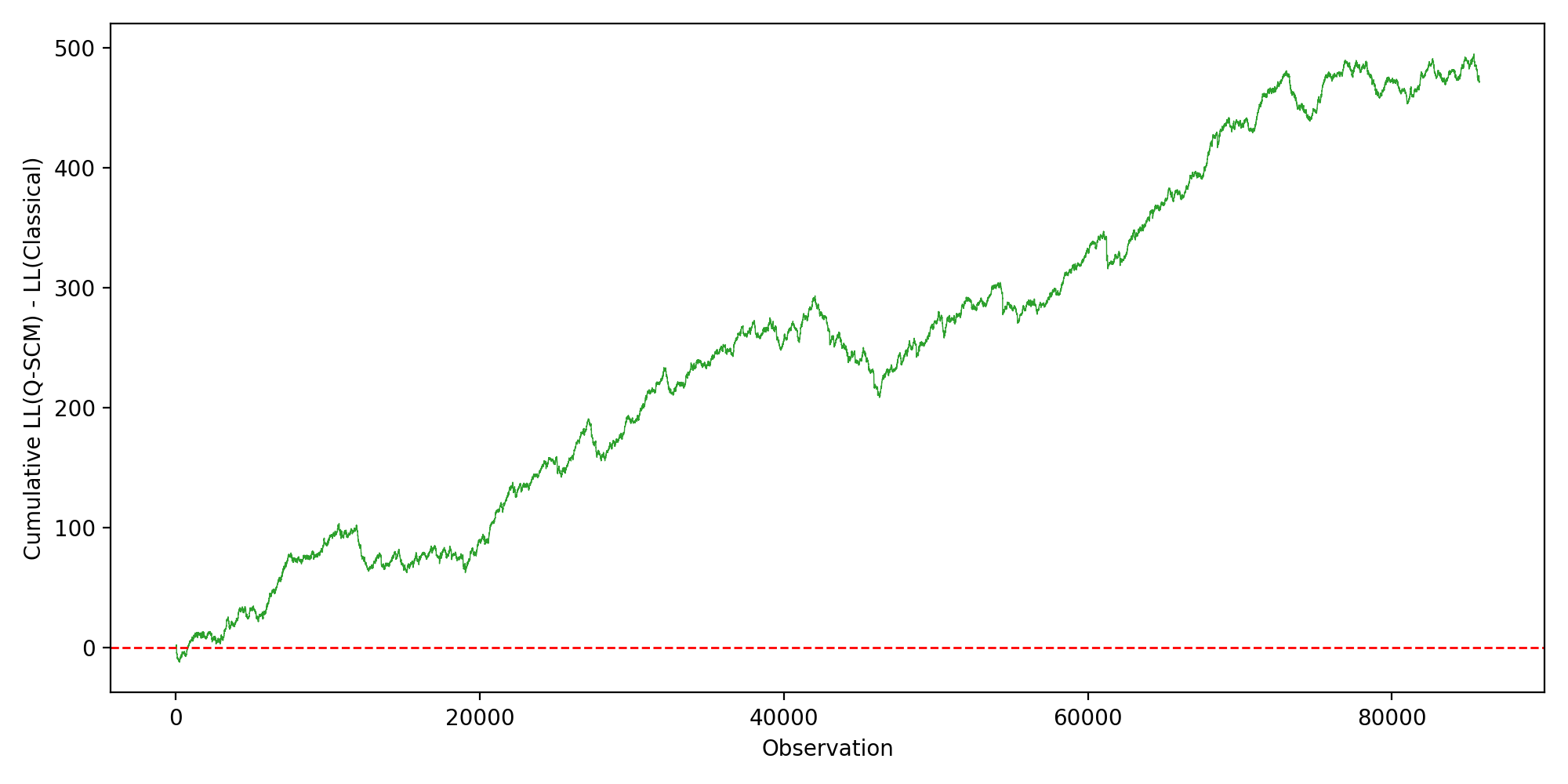
We beleive that the 471.8 LL improvement is not a consequence of the Q-SCM having strictly more parameters than the classical baseline, because the AIC penalty already adjusts for that. Rather, it identifies a real difference in the structure of the class assignment mapping. We highlight three methodological features of the Q-SCM that are absent from the classical baseline specification used here. The classical class probability $P(D_{t})$ is a function only of the contemporaneous cue $\mathrm{CTTC}_{t}$ . Two observations with identical CTTC are assigned identical $P(D)$ irrespective of the driver’s history. The Q-SCM’s $P(D_{t})$ , in contrast, is a function of the entire cue trajectory $\{s_{\mathrm{dist},s},\,s_{\mathrm{speed},s},\,s_{\mathrm{dev},s}\}_{s\leq t}$ for the driver, integrated through the recursive quantum state evolution. Under the classical baseline used in this paper, two drivers with identical CTTC at $t$ receive identical $P(D_{t})$ , even if their cue histories differ. In Q-SCM, the same two drivers can have different $P(D_{t})$ because the current state carries the accumulated effect of prior cue updates.

The aggregate gain is consistent but modest at the level of individual observations. Figure 6 shows the cumulative difference in per observation log likelihood between the two models across all $85{,}754$ observations. As can be seen fromt he figure, the curve rises steadily to its final value of $+471.8$ without large jumps. This implies that the Q-SCM advantage is broadly distributed rather than driven by a few outliers. At the same time, the per observation improvement is small on average ( $+471.8/85{,}754\approx+0.006$ ), and Q-SCM assigns a higher likelihood than the classical model to roughly $54\%$ of drivers and of observations. The contribution of Q-SCM is therefore best understood as a consistent structural improvement in the class assignment mechanism, together with a more behaviourally interpretable latent state, rather than a large gain in point wise predictive accuracy.

Unlike the classical class membership, where the effect of CTTC on class utility is controlled directly by the estimated coefficient and can change sharply from one observation to the next ,the Q-SCM updates the defensive probability by a bounded state rotations. Each cue can only move the cognitive state by a limited amount at each timestep, and the saturating response function prevents abrupt unbounded changes. The no pendulum constraint ensures that sustained threat exposure does not produce unrealistic oscillation in the defensive probability. When the threat weakens or disappears, the estimated relaxation weight $\lambda=0.44$ allows the state to move back to the neutral baseline. Hence, Q-SCM provides a smoother and more behaviourally constrained representation of how defensive state probability increases under continued threat and decreases after the threat passes.

Figure 7 shows distributions of $P(D_{t})$ for the 85,754 observations in the two models. The classical distribution is concentrated near $P(D)\approx 0.73$ with a long left tail. Since the membership utility of the Defensive class decreases when the short CTTC conflict term increases, observations with severe instantaneous conflict are shifted away from the Defensive toward the Neutral class. The Q-SCM distribution is bimodal instead. Drivers either are near $P(D)\approx 0$ or near $P(D)\approx 1$ , with intermediate probabilities representing observations during state transition. This near neutral versus near defensive separation is a direct consequence of the bounded sequential response. Once cumulative cue processing has moved the state vector close to one pole, the state tends to remain near that pole until subsequent cue evidence and relaxation move it away. The two models identify qualitatively different latent constructs. The classical construct corresponds to a default cruise mode in which deceleration is the preferred response. The Q-SCM construct corresponds to a committed response mode that drivers enter only after sufficient accumulated threat has been processed over time. Both interpretations are internally consistent, but the Q-SCM interpretation is more closely aligned with the behavioural notion of defensive driving as a state shift triggered by accumulated risk perception.

5.3 Synthetic Data Estimation

The purpose of the synthetic data estimation is to evaluate the proposed Q-SCM under a controlled setting where the true data generating mechanism is known. Unlike the empirical application where the true driver mental state process is unobserved, the synthetic experiment allows us to generate actions directly from the Q-SCM using known parameter values. This provides a way to examine whether the estimation procedure can recover the imposed Q-SCM structure. Also, whether the sequential state evolution mechanism produces behavioural patterns that are distinguishable from the classical baseline model. The synthetic dataset is generated in two stages. First, the explanatory variables are generated using a driver-level bootstrap from the rounD Neuweiler dataset. The $9{,}610$ drivers are sampled by replacing from the original set of $9{,}610$ drivers. For each sampled driver, the full observed trajectory is retained including the sequence of cue and feature variables: $(\mathrm{mDist}_{t},\mathrm{CTTC}_{t},\text{lateral deviation}_{t},o_{j,t},d_{j,t},f_{t},r_{t})$ . This step keeps the temporal structure for each driver trajectory and the empirical dependence among the variables. Because the sampling is conducted at the driver level and not the observation level, the synthetic dataset retained realistic within driver sequences. Also, because drivers are sampled with replacement the dataset is not simply a direct repllication of the empirical sample.

In the second stage, the action variable is simulated. The probabilities are evaluated using the parameter vector $\boldsymbol{\Theta}^{\star}$ estimated from the real data. The simulated actions are then treated as the dependent variable in the synthetic dataset. Finally, the Q-SCM is re-estimated using the synthetic data, and the recovered estimates are compared with the known data generating values $\boldsymbol{\Theta}^{\star}$ . Figure 8 shows the real and synthetic distributions of the cue variables, per-alternative variables and action shares. The cue and feature distributions are closely aligned in the two datasets. This implies that the driver level bootstrap reproduced the main statistical structure of the empirical data.

Table 9 shows the parameter estimation results. For each parameter, the table shows the true value that is used to generate the synthetic actions, the estimate from the synthetic data, bias and the standard error. The $t$ -statistic tests if the recovered estimate is statistically different from the true parameter value used to generate the synthetic data. The ^∗ denotes rejection at the $5\%$ level. It can be seen that the main Q-SCM parameters are generally recoverable from a dataset with the same size and temporal structure as the empirical sample. The relaxation weight $\lambda$ was recovered almost exactly and a minimal bias of $-0.0003$ . The maximum rotation parameters for the distance and deviation cues, $\theta_{\max,\mathrm{dist}}$ and $\theta_{\max,\mathrm{dev}}$ , are also recovered closely.

Table 9: Q-SCM estimates using synthetic data.

Quantum layer
Parameter	True (Empirical)	Estimate (Synthetic)	Bias	SE	$t$ -stat
$\theta_{\max,\mathrm{dev}}$	$2.6143$	$2.6033$	$-0.0110$	$0.0194$	$-0.57$
$\theta_{\max,\mathrm{dist}}$	$3.1191$	$3.1349$	$+0.0158$	$0.0699$	$+0.23$
$\theta_{\max,\mathrm{speed}}^{*}$	$1.7565$	$2.1316$	$+0.3751$	$0.0478$	$+7.85$
$k_{\mathrm{dev}}^{*}$	$1.0721$	$0.9617$	$-0.1104$	$0.0134$	$-8.26$
$k_{\mathrm{dist}}$	$0.4652$	$0.5307$	$+0.0655$	$0.0528$	$+1.24$
$k_{\mathrm{speed}}^{*}$	$1.7781$	$1.5893$	$-0.1888$	$0.0220$	$-8.57$
$\theta_{0}^{*}$	$0.0649$	$0.0796$	$+0.0147$	$0.0064$	$+2.29$
$\lambda$	$0.4415$	$0.4412$	$-0.0003$	$0.0091$	$-0.03$
Choice layer
$\beta^{N,*}_{\mathrm{decel}}$	$0.4288$	$0.3315$	$-0.0973$	$0.0234$	$-4.16$
$\beta^{N}_{\mathrm{accel}}$	$2.0198$	$2.0219$	$+0.0021$	$0.0265$	$+0.08$
$\beta^{N,*}_{\mathrm{dist\_path}}$	$-2.1288$	$-2.2058$	$-0.0770$	$0.0351$	$-2.19$
$\beta^{N}_{\mathrm{overlap}}$	$0.5190$	$0.5487$	$+0.0297$	$0.0292$	$+1.02$
$\beta^{N}_{\mathrm{int}}$	$0.3087$	$0.3156$	$+0.0069$	$0.0307$	$+0.22$
$\beta^{D,*}_{\mathrm{decel}}$	$1.8540$	$1.9421$	$+0.0881$	$0.0414$	$+2.13$
$\beta^{D}_{\mathrm{accel}}$	$-2.0404$	$-1.6706$	$+0.3698$	$0.2520$	$+1.47$
$\beta^{D}_{\mathrm{overlap}}$	$0.9378$	$1.2351$	$+0.2973$	$0.2019$	$+1.47$
$\beta^{D}_{\mathrm{int}}$	$0.3348$	$0.2732$	$-0.0616$	$0.0708$	$-0.87$

The main recovery limitation is for for the speed cue parameters, $\theta_{\max,\mathrm{speed}}$ and $k_{\mathrm{speed}}$ . The recovered value of $\theta_{\max,\mathrm{speed}}$ is higher than the true value, but the recovered value of $k_{\mathrm{speed}}$ is lower. This opposite movement is expected because the two parameters jointly determine the bounded cue response function, $\theta_{t,m}=\theta_{\max,c}\frac{s_{t,m}}{k_{c}+s_{t,m}}$ . A larger maximum rotation can be partly offset by a smaller saturation constant, producing a similar effective rotation over the observed cue range. Therefore, the bias mainly reflects a trade-off between these two parameters, rather than a failure of the Q-SCM structure. Over the observed range of speed cue values, the effective rotation implied by the recovered parameter pair remained within approximately $4\%$ of the true rotation. This suggests that the behavioural impact of this trade-off was limited. The choice layer parameters are also mostly recovered well. Most coefficients were within their driver clustered standard errors of the true values. Only two coefficients, $\beta^{N}_{\mathrm{decel}}$ and $\beta^{N}_{\mathrm{dist\_path}}$ , rejected the t-test at the $5\%$ level, and their biases were modest. The largest absolute coefficient difference was observed for $\beta^{D}_{\mathrm{accel}}$ , but this estimate did not reject the true value once driver-level uncertainty is considered.

The synthetic analysis also provides a useful check on the model comparison. Since synthetic actions are generated from Q-SCM, the classical latent class specification is misspecified is the synthetic data generation and is expected to fit worse than Q-SCM. Table 10 shows the goodness of fit comparison where Q-SCM has a log-likelihood of $-63{,}513.8$ , compared with $-65{,}377.0$ for the classical baseline. This gain is substantially larger than the $+471.8$ log-likelihood advantage observed on the empirical data (Table 5), which is the expected pattern when the data generating process follows Q-SCM. In synthetic data, the classic model has no path to recover the path dependent latent state mechanism that generated the actions, so the structural advantage of Q-SCM is amplified.

Table 10: Goodness of fit for the synthetic dataset.

Model	Log Likelihood	$df$	AIC	BIC	$\rho^{2}$
Q-SCM	$-63{,}513.84$	$17$	$127{,}061.69$	$127{,}220.76$	$0.3244$
Classical	$-65{,}376.97$	$11$	$130{,}775.94$	$130{,}878.86$	$0.3046$
$\Delta$	$+1{,}863.13$	$+6$	$-3{,}714.25$	$-3{,}658.10$	$+0.0198$

Table 11 shows the parameter estimates for the classical model using the synthetic data besides the empirical classical estimates added here for reference. Several coefficients shift substantially relative to the empirical fit. The class membership coefficient on CTTC shrinks from $\hat{\gamma}_{1}=-4.44$ on the empirical data to $\hat{\gamma}_{1}^{\mathrm{synth}}=-0.79$ on the synthetic data, and the class-membership constant shrinks from $\hat{\gamma}_{2}=1.01$ to $\hat{\gamma}_{2}^{\mathrm{synth}}=0.16$ . The within-state acceleration constant in the neutral class is also attenuated ( $\hat{\beta}^{N}_{\mathrm{accel}}$ moves from $5.74$ to $3.06$ ), as is the path-deviation coefficient ( $-5.71$ to $-2.86$ ). Two complementary interpretations are consistent with these shifts. First, the classical model can use only a contemporaneous-CTTC class equation, so when the synthetic actions encode information from the full cue history the classical model has no covariate that captures it and the CTTC coefficient is correspondingly weakened. Second, the within-state utilities are biased because the classical model is assigning observations to the Neutral/Defensive classes using a different rule than the one that generated the data; the within-state estimates therefore reflect a mixture across cognitive states rather than the state-pure estimates that Q-SCM identifies. Both interpretations point to the same conclusion: the empirical fit gap between Q-SCM and the classical baseline reported in Section 5 is not a numerical artefact, and the classical model’s apparent strength on the empirical data is partly due to parameters compensating for the missing dynamic mechanism. There is no “true value” column because the classical specification is not the data generating process; instead the rightmost column reports the empirical classical estimate from Table 7 and Table 8 for reference.

Table 11: Classical model estimates using synthetic data.

Within-state choice utility
Parameter	True (Empirical)	Estimate (synthetic)	SE	p-value
$\beta^{N}_{\mathrm{decel}}$	$-0.1422$	$0.3339$	$0.0679$	$<0.001$
$\beta^{N}_{\mathrm{accel}}$	$5.7358$	$3.0579$	$0.1011$	$<0.001$
$\beta^{N,*}_{\mathrm{dist\_path}}$	$-5.7142$	$-2.8618$	$0.0879$	$<0.001$
$\beta^{N}_{\mathrm{overlap}}$	$0.6494$	$0.8260$	$0.0429$	$<0.001$
$\beta^{N}_{\mathrm{int}}$	$0.5562$	$0.1707$	$0.0446$	$<0.001$
$\beta^{D,*}_{\mathrm{decel}}$	$1.3543$	$1.5614$	$0.0430$	$<0.001$
$\beta^{D}_{\mathrm{accel}}$	$-1.7118$	$-1.6638$	$0.1482$	$<0.001$
$\beta^{D}_{\mathrm{overlap}}$	$0.4611$	$0.6837$	$0.1468$	$<0.001$
$\beta^{D,*}_{\mathrm{int}}$	$0.1654$	$0.3598$	$0.0600$	$<0.001$
Class membership
$\gamma_{1}$ (CTTC coefficient)	$-4.4431$	$-0.7893$	$0.1251$	$<0.001$
$\gamma_{2}$ (constant)	$1.0134$	$0.1602$	$0.0401$	$<0.001$

6 Conclusions

This paper present the Q-SCM which is a driver behaviour framework grounded in quantum cognition theory that represents the driver’s evolving mental state as a quantum state vector on the Bloch sphere. The key methodological contribution is the integration of sequential unitary rotations, governed by the Pauli matrices, with a classical MNL choice layer. This produce a two stage architecture in which the quantum state evolution determines the mixing weights between neutral and defensive behavioural regimes. Since that the quantum mechanism is confined to the class membership layer while the action choice layer remains a classical RUM, Q-SCM retains the interpretability and welfare-analytic properties (at the choice layer) of standard discrete choice models. This is in contrast to existing quantum choice models, which replace or modify the choice probabilities directly.

We provide two formal guarantees that ensure well behaved state evolution. The no-pendulum theorem shows that the monotonicity constraint eliminates oscillatory overshoot unconditionally, for any parameter values and any cue trajectory. The geodesic safeguard mechanism guarantees convergence toward the target pole under sustained threat, resolving the stalling problem that arises from fixed axis rotations near the poles of the Bloch sphere. The model was estimated on 85,754 observations from 9,610 drivers in the rounD naturalistic roundabout dataset. Compared with a classical latent class baseline using the identical within-state choice utility, the Q-SCM achieves a log-likelihood advantage compared to the classical baseline. The advantage is broadly distributed across observations. The Q-SCM had a better fit than the classical latent class benchmark using the same conditional choice utility specification. This improvement is attributed to the different mechanism used to generate the neutral and defensive state probabilities. In the classical model, state probabilities are generated from a memoryless contemporaneous membership function. In Q-SCM, they are generated by the sequential quantum state evolution, where the current state carries the accumulated influence of previous cue exposure. The inferred Q-SCM trajectories exhibit the behavioural properties targeted by the proposed framework. These include bounded cue response, gradual movement toward the defensive state under sustained threat exposure, persistence of the defensive state after the threat weakens, and relaxation toward the neutral baseline when the threat weakens. These properties do not emerge naturally from the classical benchmark unless additional dynamic structure, constraints, or history dependent variables are introduced. In the synthetic data analysis, the cue variables were drawn from the empirical rounD trajectories. The actions were simulated from the Q-SCM using the estimated real data parameters. The model recovered the main quantum layer and choice layer parameters, with the main limitation being a partial trade-off between $\theta_{\max,c}$ and $k_{c}$ for the speed cue. The estimation shows a partial trade off between $\theta_{\max,c}$ and $k_{c}$ for the speed cue, which is expected feature of the bounded response saturating function and does not materially affect the rotation produced over the observed cue range. The model comparison advantage of Q-SCM over the classical baseline is larger on the synthetic dataset than on the real data. It is an expected behaviour when the data generation is Q-SCM and supports the structural interpretation of the real data fit improvement.

Several directions for future work are identified. The current model is restricted to $K=2$ cognitive states (neutral and defensive), which admits the Bloch sphere as a geometric visualization of the state space. Extending to $K>2$ states such as including an aggressive or distracted mode alongside neutral and defensive would require moving from the Bloch sphere to the full $K$ -dimensional complex Hilbert space $\mathcal{H}_{K}$ . In this generalization, the state vector $\left|\psi\right\rangle\in\mathbb{C}^{K}$ with $\|\psi\|=1$ lives on the surface of a $(2K-1)$ -dimensional unit sphere, and cue updates are generated by the $K^{2}-1$ generalized Gell-Mann matrices rather than the three Pauli matrices. While the geometric intuition of the Bloch sphere is lost for $K>2$ , the algebraic structure of unitary rotations, non commutativity, and interference carries over directly. The choice layer would generalize to a $K$ -component mixture $P(a_{t})=\sum_{k=1}^{K}P(a_{t}\mid S_{k})\,P(S_{k})_{t}$ , with the mixing weights determined by the quantum state evolution. The challenges here become more computational (the number of generators grows as $K^{2}-1$ ) and empirical (identifying and interpreting the additional cognitive modes from observed driving actions).

The current specification assumes homogeneous parameters across all drivers. Every driver shares the same rotation magnitudes, sensitivity parameters, and choice coefficients. This assumption can be relaxed by introducing random parameters in the spirit of mixed logit models. Driver specific coefficients may capture heterogeneity in both the means and variances of behavioural responses. This allows some drivers to be inherently more reactive to state changing cues, while others may be more sensitive to the phase changing cue. Similarly, driver specific rotation parameters would allow heterogeneity in cognitive sensitivity to cue changes on the Bloch sphere. Estimating such models would require simulation based maximum likelihood or hierarchical Bayesian methods, which integrate over the distribution of individual level parameters. This extension would separate within driver state dynamics (captured by the quantum evolution) from between driver heterogeneity (captured by the random parameter distributions). We emphasize that such a random parameters extension addresses a different axis of richness than the sequential mechanism studied here. It captures between driver heterogeneity, whereas the quantum layer captures within driver cue history dependence. The two are complementary, and placing random parameters on the quantum layer would combine both.

Another extension that can be implemented is related to the order in which cues are processed within each time step. The current model uses a fixed processing sequence (separation distance, closing speed, then lateral deviation) which is identical across all drivers and all time steps. This simplification seems appropriate for establishing the framework, however, it does not capture the possibility that drivers may prioritize cues based on their momentary salience. An attentionally driven ordering where the cues are processed in decreasing order of their instantaneous change magnitude $|\Delta s_{t,m}|$ , would allow the most threatening or rapidly changing cue to be evaluated first. Since $\sigma_{x}$ and $\sigma_{z}$ rotations do not commute, such reordering would have different state trajectories and different defensive probabilities for the same set of cue values. This would make the interference structure of the model sensitive to attentional prioritization. This extension would introduce a data driven processing sequence where the order effects will vary across observations and drivers. This will produce a richer but more complex account of sequential cue integration.

Acknowledgments

The first author is funded by the Canada Postdoctoral Research Award (CPRA) through the Natural Sciences and Engineering Research Council of Canada (NSERC). First and second authors are funded by the Canada Research Chair program in Disruptive Transportation Technologies and Services (CRC-2021-00480).

Appendix A Bloch Sphere Representation

The Bloch sphere provides a geometric visualization of the two-state quantum system. The north pole corresponds to $\left|N\right\rangle$ (neutral state) and the south pole corresponds to $\left|D\right\rangle$ (defensive state), as shown in Figure 3. The polar angle $\theta$ (distinct from the per-update rotation angle $\theta_{t,m}$ introduced in Section 3.3) determines $P(D)=\sin^{2}(\theta/2)$ , while the azimuthal angle $\phi$ encodes the phase. Intuitively, the phase represents the driver’s latent cognitive context. It is the accumulated influence of prior cues that is not visible in the current defensive probability but affects how the driver responds to future cues. Two drivers with the same $P(D)$ coul have arrived at that state through different cue histories. For instance, one driver may process a phase changing cue, while another may process only state changing cues. Their defensive probabilities are equal while their phases are not, and the same subsequent state changing cue can move them to different states on the sphere. Therefore, the phase can be seen as a form of cognitive memory that is hidden from any single observation but revealed by its effect on subsequent responses.

Any pure two-state cognitive state can be written as:

\left|\psi\right\rangle=\alpha\left|N\right\rangle+\beta\left|D\right\rangle,\qquad|\alpha|^{2}+|\beta|^{2}=1,

(31)

where $\alpha$ and $\beta$ are complex probability amplitudes associated with the neutral and defensive states, respectively. $|\cdot|$ is the modulus of a complex number. Using the standard Bloch sphere parameterization, the same state can be written as:

\left|\psi\right\rangle=\cos\left(\frac{\theta}{2}\right)\left|N\right\rangle+e^{i\phi}\sin\left(\frac{\theta}{2}\right)\left|D\right\rangle,

(32)

where $\theta\in[0,\pi]$ is the polar angle measured from the neutral pole and $\phi\in[0,2\pi)$ is the azimuthal angle representing the relative phase between the neutral and defensive components. Equivalently,

\alpha=\cos\left(\frac{\theta}{2}\right),\qquad\beta=e^{i\phi}\sin\left(\frac{\theta}{2}\right).

(33)

The squared moduli of the amplitudes give the probabilities of the two cognitive states:

P(N)=|\alpha|^{2}=\cos^{2}\left(\frac{\theta}{2}\right),\qquad P(D)=|\beta|^{2}=\sin^{2}\left(\frac{\theta}{2}\right)=\frac{1-\cos(\theta)}{2}.

(34)

Hence, the polar angle $\theta$ determines the driver’s position on the neutral–defensive spectrum. For instance, a driver with $|\beta|^{2}=0.3$ has a 30% probability of being in the defensive state and a 70% probability of being in the neutral state. The phase $\phi$ does not change these probabilities at a single observation, but it affects how the state responds to subsequent cue induced rotations.

The state vector in Eq. (31) is a pure state, representing a fully specified superposition that lies on the surface of the Bloch sphere. The present model operates entirely using pure states. In contrast, a mixed state represents classical uncertainty about which pure state the system occupies. For example, if there is a 60% chance that the driver is in pure state $\left|\psi_{1}\right\rangle$ and a 40% chance that the driver is in pure state $\left|\psi_{2}\right\rangle$ , the mixture is described by the density matrix

\rho=0.6\left|\psi_{1}\right\rangle\!\left\langle\psi_{1}\right|+0.4\left|\psi_{2}\right\rangle\!\left\langle\psi_{2}\right|.

(35)

On the Bloch sphere, a pure state lies on the surface with $\|\mathbf{r}\|=1$ , whereas a mixed state lies inside the sphere with $\|\mathbf{r}\|<1$ [15]. The pure state assumption is appropriate here because each driver trajectory is treated as a single realization in which the driver begins from an initialized cognitive state and then receives deterministic cue updates over time.

The state can also be mapped to a Bloch vector $\mathbf{r}=(r_{x},r_{y},r_{z})$ by taking the expectation value of each Pauli matrix with respect to the current state:

r_{x}=\left\langle\psi\right|\sigma_{x}\left|\psi\right\rangle,\qquad r_{y}=\left\langle\psi\right|\sigma_{y}\left|\psi\right\rangle,\qquad r_{z}=\left\langle\psi\right|\sigma_{z}\left|\psi\right\rangle,

(36)

where $\boldsymbol{\sigma}=(\sigma_{x},\sigma_{y},\sigma_{z})$ are the Pauli matrices. Each component measures the alignment of the state with the corresponding axis of the Bloch sphere. The $r_{z}$ component determines the neutral and defensive probabilities through the Born rule:

P(N)=\frac{1+r_{z}}{2},\qquad P(D)=\frac{1-r_{z}}{2}.

(37)

The remaining components, $r_{x}$ and $r_{y}$ , encode the phase information that is not visible from $P(D)$ alone but influences later state evolution.

Appendix B Unitary Rotations on the Bloch Sphere

Unitary transformations on a two-state system are rotations on the Bloch sphere. The fundamental generators of all such rotations are the three Pauli matrices:

\sigma_{x}=\begin{pmatrix}0&1\\ 1&0\end{pmatrix},\quad\sigma_{y}=\begin{pmatrix}0&-i\\ i&0\end{pmatrix},\quad\sigma_{z}=\begin{pmatrix}1&0\\ 0&-1\end{pmatrix}.

(38)

Any rotation on the Bloch sphere can be built by combining $\sigma_{x}$ , $\sigma_{y}$ , and $\sigma_{z}$ in appropriate proportions [15]. In the most general case, a rotation around an arbitrary axis $\hat{\mathbf{n}}=(n_{x},n_{y},n_{z})$ with $\|\hat{\mathbf{n}}\|=1$ is

U_{\hat{\mathbf{n}}}(\theta)=\exp\!\left(-i\frac{\theta}{2}\,\hat{\mathbf{n}}\cdot\boldsymbol{\sigma}\right)=\cos\!\left(\frac{\theta}{2}\right)I-i\sin\!\left(\frac{\theta}{2}\right)\!\left(n_{x}\sigma_{x}+n_{y}\sigma_{y}+n_{z}\sigma_{z}\right),

(39)

which reduces, when the axis is aligned with a coordinate direction, to the single axis rotation

U_{a}(\theta)=\exp\!\left(-i\frac{\theta}{2}\sigma_{a}\right)=\cos\!\left(\frac{\theta}{2}\right)I-i\sin\!\left(\frac{\theta}{2}\right)\sigma_{a},\qquad a\in\{x,y,z\}.

(40)

The $\sigma_{x}$ and $\sigma_{y}$ components mix the amplitudes $\alpha$ and $\beta$ between $\left|N\right\rangle$ and $\left|D\right\rangle$ , directly altering $P(D)=|\beta|^{2}$ . The $\sigma_{z}$ component $U_{z}(\theta)=\mathrm{diag}(e^{-i\theta/2},e^{i\theta/2})$ multiplies each amplitude by a phase factor and leaves $|\alpha|^{2}$ and $|\beta|^{2}$ unchanged. Starting from the neutral pole $\left|N\right\rangle$ (Figure 9):

•

$\sigma_{x}$ rotation (state change, imaginary amplitude): $U_{x}(\theta)\left|N\right\rangle=\cos(\theta/2)\left|N\right\rangle-i\sin(\theta/2)\left|D\right\rangle$ , giving $P(D)=\sin^{2}(\theta/2)$ .
•

$\sigma_{z}$ rotation (phase change only): $U_{z}(\theta)\left|N\right\rangle=e^{-i\theta/2}\left|N\right\rangle$ , giving $P(D)=0$ .
•

$\sigma_{y}$ rotation (state change, real amplitude): $U_{y}(\theta)\left|N\right\rangle=\cos(\theta/2)\left|N\right\rangle+\sin(\theta/2)\left|D\right\rangle$ , giving $P(D)=\sin^{2}(\theta/2)$ as well, with a purely real $\left|D\right\rangle$ amplitude.

In Q-SCM, each cue type is assigned to exactly one of two Pauli axes. The $\sigma_{x}$ axis is reserved for cues that directly change the defensive probability (state change) and the $\sigma_{z}$ axis for cues that modulate the internal phase without directly altering $P(D)$ (phase change). No cue is assigned to $\sigma_{y}$ , and no cue induces a rotation around a general off-axis direction. This assumption is motivated by three considerations. First, the two retained axes capture the two fundamental and distinct ways a cue can influence cognition. A $\sigma_{z}$ cue can be understood as a priming or context-setting signal which does not, by itself, make the driver more or less defensive but conditions how subsequent state-changing cues are processed. Second, confining each cue to a single axis yields a parsimonious model with clear cognitive interpretation, and the model parameters (axis assignment and rotation magnitude) are directly identifiable. Third, the $\sigma_{y}$ axis simultaneously produces both state and phase change, coupling the two mechanisms in a way that increases model complexity without a clear cognitive justification at this stage. When two cues on different axes ( $\sigma_{x}$ and $\sigma_{z}$ ) are composed sequentially, the resulting product rotation generically contains a $\sigma_{y}$ component, a direct consequence of the commutation relation $[\sigma_{x},\sigma_{z}]=-2i\sigma_{y}$ . Therefore, combined state and phase effects emerge naturally from the sequential composition of cue updates rather than being assigned to individual cues. We adopt $\sigma_{x}$ as the state changing axis and $\sigma_{z}$ as the phase changing axis; the specific assignment of driving cues to these axes is detailed in Section 3.3.

Appendix C Formal Guarantees

C.1 Proof of Theorem 1

With the monotonicity constraint applied, the defensive probability is non decreasing across the cue driven evolution, regardless of the maximum rotation $\theta_{\max,c}$ or the initial state. Formally, let $P_{D}^{(m)}$ denote the value of $P(D)$ after the first $m$ rotations at step $t$ . Then:

(i)

Stationarity: if $s_{t,m}=0$ for all cues $m$ at step $t$ , then $\theta_{t,m}=0$ for all $m$ and $\left|\psi_{t}\right\rangle=\left|\psi_{t,0}\right\rangle$ . The state is unchanged.
(ii)

Threat monotonicity: every applied threat rotation ( $\theta_{t,m}>0$ ) satisfies

$P_{D}^{(m)}\;\geq\;P_{D}^{(m-1)}.$
(iii)

No pendulum: during any contiguous sequence of non zero cues ( $s_{t,m}>0$ for all $m$ at every step) the sequence $\{P_{D}^{(m)}\}$ is non decreasing across all cues and steps. It cannot exhibit the increase-then-decrease oscillation characteristic of pendulum overshoot.

Proof.

(i) $s=0$ gives $\tau=0/(k+0)=0$ , hence $\theta=\theta_{\max}\cdot 0=0$ . Therefore $U_{\mathfrak{a}}(0)=I$ and the state is unchanged.

(ii) Let $\left|\psi\right\rangle$ be the state before cue $m$ , with $P_{D}=|\left\langle D\middle|\psi\right\rangle|^{2}$ . The trial state is $\left|\psi^{\prime}\right\rangle=U_{\mathfrak{a}(c_{t,m})}(\theta_{t,m})\,\left|\psi\right\rangle$ with $P_{D}^{\prime}=|\left\langle D\middle|\psi^{\prime}\right\rangle|^{2}$ . By Eq. 11: if $\theta_{t,m}>0$ and $P_{D}^{\prime}<P_{D}$ , the rotation is skipped and $P_{D}^{(m)}=P_{D}^{(m-1)}$ . Otherwise it is applied and $P_{D}^{(m)}=P_{D}^{\prime}\geq P_{D}^{(m-1)}$ . In either case, $P_{D}^{(m)}\geq P_{D}^{(m-1)}$ .

(iv) During such a sequence, $s_{t,m}>0$ for all $m$ , so $\theta_{t,m}>0$ . By (i), cues with $s=0$ preserve $P_{D}$ . By (ii), cues with $\theta>0$ yield $P_{D}^{(m)}\geq P_{D}^{(m-1)}$ . Composing across all cues and steps, $P_{D}$ is non decreasing throughout the sequence. A non decreasing sequence cannot first increase then decrease, excluding the pendulum pattern.

∎

C.2 Proof of Proposition 1

Formally, under Eq. 15:

(i)

No overshoot: all guarantees of Theorem 1 are preserved. In particular, $P(D)$ is non decreasing at every step.
(ii)

Strict progress: if $\theta_{t,m}\neq 0$ and the current state is not already at the target pole, then $P_{D}^{(m)}\neq P_{D}^{(m-1)}$ : the state strictly advances toward the target.
(iii)

Convergence: during any sustained worsening sequence ( $s_{n}>0$ for all $n$ ), $P(D)$ converges monotonically toward $1$ . The state cannot stall at any intermediate value.

Proof.

(i) When the Pauli rotation moves $P(D)$ in the correct direction, it is applied unchanged and the guarantees of Theorem 1 hold directly. When the geodesic safeguard is used, the rotation axis is chosen to move $\mathbf{r}$ toward the target pole, and the angle is constrainted to $\min(\theta_{t,m},\phi)$ . Since $\phi$ is the exact angular distance to the pole, rotating by at most $\phi$ cannot pass the pole. Therefore $P(D)$ cannot decrease at any step.

(ii) If the Pauli rotation is accepted, it moves $P(D)$ in the correct direction by assumption, so $P_{D}^{(m)}\neq P_{D}^{(m-1)}$ . If the geodesic safeguard is used, the applied angle is $\theta_{\mathrm{geo}}=\min(\theta_{t,m},\phi)$ . Since $\theta_{t,m}>0$ and $\phi>0$ (the state is not at the pole), we have $\theta_{\mathrm{geo}}>0$ . By construction, the geodesic rotation by any positive angle strictly decreases the angular distance to the target pole, so $P(D)$ strictly increases.

(iii) During sustained worsening, $s_{n}\geq s_{\min}>0$ for all $n$ , hence $\tau_{n}\geq s_{\min}/(s_{\min}+k)>0$ and $\theta_{n}\geq\theta_{\min}:=\theta_{\max}\,s_{\min}/(s_{\min}+k)>0$ . By (ii), each step strictly increases $P(D)$ . The sequence $\{P(D)_{n}\}$ is strictly increasing and bounded above by $1$ , so by the monotone convergence theorem it converges to some limit $L\leq 1$ . Suppose for contradiction that $L<1$ . Then the angular distance $\phi_{n}=\arccos(-r_{z,n})$ remains bounded below by some $\phi^{*}>0$ for all $n$ . At each step, the applied geodesic rotation is $\theta^{\mathrm{geo}}_{n}=\min(\theta_{n},\phi_{n})\geq\min(\theta_{\min},\phi^{*})>0$ , which produces a strictly positive increment in $P(D)$ bounded below by a constant $\Delta>0$ depending only on $\theta_{\min}$ and $\phi^{*}$ . After finitely many steps the cumulative increment exceeds the remaining gap $1-L$ , contradicting $P(D)_{n}\to L<1$ . Therefore $L=1$ . ∎

References

[1] D. Aerts and S. Sozzo (2014) Quantum entanglement in concept combinations. International Journal of Theoretical Physics 53, pp. 3587–3603. Cited by: §1.
[2] R. Al-Haideri, K. Ismail, B. Farooq, and A. Weiss (2026) Modelling driver behaviour as a continuum between defensive and neutral states. Transportation Research Part F: Traffic Psychology and Behaviour 121, pp. 103694. Cited by: §1, §4.1, §4.2.1, §5.
[3] V. Bergholm, J. Izaac, M. Schuld, C. Gogolin, S. Ahmed, V. Ajith, M. S. Alam, et al. (2018) PennyLane: automatic differentiation of hybrid quantum-classical computations. External Links: 1811.04968 Cited by: §5.
[4] P. D. Bruza, Z. Wang, and J. R. Busemeyer (2015) Quantum cognition: a new theoretical approach to psychology. Trends in Cognitive Sciences 19, pp. 383–393. Cited by: §1, §1.
[5] J. R. Busemeyer and P. D. Bruza (2012) Quantum models of cognition and decision. Cambridge University Press, Cambridge. Cited by: §3.3.
[6] J. R. Busemeyer and Z. Wang (2015) What is quantum cognition, and how is it applied to psychology?. Current Directions in Psychological Science 24 (3), pp. 163–169. Cited by: §1, §1.
[7] M. Di Gangi and A. Vitetta (2021) Quantum utility and random utility model for path choice modelling: specification and aggregate calibration from traffic counts. Journal of Choice Modelling 40, pp. 100290. External Links: Document, ISSN 1755-5345 Cited by: Table 1, §2, §2.
[8] G. P. Epping, P. D. Kvam, T. J. Pleskac, and J. R. Busemeyer (2023) Open system model of choice and response time. Journal of Choice Modelling 49, pp. 100453. External Links: Document, ISSN 1755-5345 Cited by: Table 1, §2.
[9] W. H. Greene and D. A. Hensher (2003) A latent class model for discrete choice analysis: contrasts with mixed logit. Transportation Research Part B: Methodological 37 (8), pp. 681–698. Cited by: §1, §3.
[10] T. O. Hancock, J. Broekaert, S. Hess, and C. F. Choudhury (2020) Quantum choice models: a flexible new approach for understanding moral decision-making. Journal of Choice Modelling 37, pp. 100235. External Links: Document Cited by: Table 1, §2.
[11] T. O. Hancock, J. Broekaert, S. Hess, and C. F. Choudhury (2020) Quantum probability: a new method for modelling travel behaviour. Transportation Research Part B: Methodological 139, pp. 165–198. Cited by: Table 1, §2.
[12] C. R. Harris, K. J. Millman, S. J. van der Walt, R. Gommers, P. Virtanen, D. Cournapeau, E. Wieser, et al. (2020) Array programming with NumPy. Nature 585 (7825), pp. 357–362. Cited by: §5.
[13] R. Krajewski, T. Moers, J. Bock, L. Vater, and L. Eckstein (2020) The round dataset: a drone dataset of road user trajectories at roundabouts in germany. In 2020 IEEE 23rd International Conference on Intelligent Transportation Systems (ITSC), Cited by: §4.1.
[14] S. Lipovetsky (2018) Quantum paradigm of probability amplitude and complex utility in entangled discrete choice modeling. Journal of Choice Modelling 27, pp. 62–73. Cited by: Table 1, §2.
[15] M. A. Nielsen and I. L. Chuang (2010) Quantum computation and quantum information. 10th Anniversary edition, Cambridge University Press, Cambridge. Cited by: Appendix A, Appendix B, §3.
[16] E. M. Pothos and J. R. Busemeyer (2013) Can quantum probability provide a new direction for cognitive modeling?. Behavioral and Brain Sciences 36 (3), pp. 255–327. Cited by: §1, §1, §1.
[17] E. M. Pothos and J. R. Busemeyer (2022) Quantum cognition. Annual Review of Psychology 73, pp. 749–778. Cited by: §1.
[18] J. S. Trueblood and J. R. Busemeyer (2011) A quantum probability account of order effects in inference. Cognitive Science 35, pp. 1518–1552. Cited by: §1.
[19] P. Virtanen, R. Gommers, T. E. Oliphant, M. Haberland, T. Reddy, D. Cournapeau, E. Burovski, et al. (2020) SciPy 1.0: fundamental algorithms for scientific computing in Python. Nature Methods 17 (3), pp. 261–272. Cited by: §5.
[20] A. Vitetta (2016) A quantum utility model for route choice in transport systems. Travel Behaviour and Society 3, pp. 29–37. Cited by: Table 1, §2, §2.
[21] Z. Wang and J. R. Busemeyer (2013) A quantum question order model supported by empirical tests of an a priori and precise prediction. Topics in Cognitive Science 5, pp. 689–710. Cited by: §1.
[22] Z. Wang, T. Solloway, R. M. Shiffrin, and J. R. Busemeyer (2014) Context effects produced by question orders reveal quantum nature of human judgments. Proceedings of the National Academy of Sciences 111 (26), pp. 9431–9436. Cited by: §1, §3.3.
[23] J. G. Yu and R. Jayakrishnan (2018) A quantum cognition model for bridging stated and revealed preference. Transportation Research Part B: Methodological 118, pp. 263–280. Cited by: Table 1, §2.

$\displaystyle\left\|\psi_{t,1}\right\rangle$	$\displaystyle=U_{x}(\theta_{t,0})\,\left\|\psi_{t,0}\right\rangle,$	(27)
$\displaystyle\left\|\psi_{t,2}\right\rangle$	$\displaystyle=U_{x}(\theta_{t,1})\,\left\|\psi_{t,1}\right\rangle,$	(28)
$\displaystyle\left\|\psi_{t,3}\right\rangle$	$\displaystyle=U_{z}(\theta_{t,2})\,\left\|\psi_{t,2}\right\rangle,$	(29)