subsection \nouppercaseheads\makeevenheadheadings1 \makeoddheadheadings1
![[Uncaptioned image]](/html/2607.11938/assets/figures/bookcover.png)
Mathematics of Data Science
. Preprint: version 1.1-
Chapter 0 Notes on this Version and Current Status
This is a preprint of a book in preparation by the authors.
We anticipate the focus and content of this manuscript
not to change except for the correction of typos and other errors and other minor changes such as including additional homework problems. It can
already by used as textbook for a graduate course in Mathematics of Data Science; it has been used as such by the authors at their home institutions.
We welcome suggestions and comments, and would like to learn about any possible errors and typos.
Please contact the authors at bandeira@math.ethz.ch,
strohmer@math.ucdavis.edu, or amits@math.princeton.edu. In fact, this version was improved using many suggestions sent from, and typos found by, many students and readers. Thank you!
Thank you,
Afonso, Thomas, and Amit.
Chapter 1 Introduction
1 Origins
The idea of this book emerged from the classes on ‘‘mathematics of data science’’ that the authors have been teaching at their home institutions Princeton University (AS), UC Davis (TS), and MIT, NYU, and ETH (ASB)11 1 Lecture notes from these classes also contain a list of mathematical open problems [49], which has now helped to inspire a mathematical blog of open problems at https://randomstrasse101.math.ethz.ch/. The open problems of 2024 are available at [48].. The lecture notes eventually became the basis to this book. While there are specialized books and many advanced research papers on each topic covered in this book, we believe it fills in the gap of being a single source that provides an accessible entry point at an advanced undergraduate, or graduate, level to mathematics of data science. The book can serve readers as a segue to those more advanced and specialized topis. In that light, one of the main purposes of this book is to be used as a textbook at both the (advanced) undergraduate and graduate levels. This book also differs from most texts in the way that it interweaves mathematical theory with some of its applications in data science.
2 The data science revolution
The data science revolution is one of the most profound shifts in modern history, reshaping industries, economies, and societies with unprecedented speed and scale. At its core, the data science revolution is driven by the exponential growth in data, advances in computing power, and the development of sophisticated analytical techniques.
Data science and its cousin artificial intelligence have become a cornerstone of modern decision-making and innovation, penetrating almost all aspects of our life. In healthcare, for example, data science is driving personalized medicine and predictive analytics. By analyzing patient data, healthcare providers can tailor treatments to individual needs, predict potential health issues before they arise, and improve patient outcomes. In finance, data science is revolutionizing risk management, fraud detection, and investment strategies. Algorithms analyze market trends, assess creditworthiness, and identify unusual transactions to mitigate risks and enhance decision-making.
Retailers leverage data science to understand consumer behavior, optimize supply chains, and personalize marketing efforts. The transportation industry benefits from data science through advancements in autonomous vehicles, route optimization, and predictive maintenance. Companies use data to enhance logistics, reduce costs, and improve safety. The energy sector uses data science to optimize resource allocation, predict equipment failures, and enhance energy efficiency. Data-driven insights help in managing renewable energy sources and reducing environmental impact.
From the statistical techniques that form the basis of data analysis to the complex algorithms that power machine learning and artificial intelligence, mathematics is at the heart of data science. Understanding the connection between data science and mathematics is crucial for appreciating the depth and breadth of this revolution.
3 Mathematics as a foundation of data science
Data science is an inherently interdisciplinary field that merges techniques from mathematics, statistics, computer science, signal processing, and domain-specific knowledge to extract insights from data. However, at its core, data science is fundamentally about understanding and leveraging patterns in data. This understanding is built on a complex and nuanced foundation of mathematical principles that enable the development of models and algorithms capable of making sense of complex datasets. This book aims to unravel many of these mathematical principles and provide a thorough grounding in the essentials of data science from a rigorous, mathematical perspective.
Mathematics provides the language and framework for formalizing the processes involved in data analysis, from data collection and preprocessing to modeling and evaluation. It offers the tools necessary for designing effective algorithms, making precise predictions, visualizing complex datasets, quantifying uncertainty, and interpreting the results of data-driven experiments. As the field of data science keeps evolving at a rapid speed, new algorithms and techniques are constantly being developed. A strong mathematical foundation enables practitioners to quickly understand and adopt these innovations because they can grasp the underlying principles rather than just following black-box implementations. Moreover, with a solid grasp of mathematics, learning new methods becomes easier.
Also, when algorithms fail to produce correct results in real world applications, we would like to know why they failed. Is it because of mistakes in the experimental setup, did we gather the wrong kind of data, do we have insufficient data, is it because of corrupted measurements, calibration errors, or incorrect modeling assumptions, or perhaps due to fundamentally unrealistic expectations, or is it due to a deficiency of the algorithm itself? If it is the latter, can it be fixed by a better initialization, a more careful tuning of the parameters, or by choosing a different algorithm? Or is a more fundamental modification required, such as developing a different model, including additional prior information, taking more measurements, or a better compensation of calibration errors? How reliable are our algorithms to small changes in the input data and can we explain why an algorithm arrives at a certain prediction?
As we are dealing with larger datasets and we aim for faster and faster throughput, it becomes increasingly important to address the aforementioned challenges in a systematic and principled manner. Thus, a rigorous and thorough study of computational algorithms both from a theoretical and numerical viewpoint is not a luxury, but emerges as an imperative ingredient towards effective data-driven discovery.
While a thorough mathematical framework can never completely avoid some guessing and trial-and-error, it can dramatically reduce the time and resources we spend on trial-and-error. Good mathematical theory can help in predicting if a problem is solvable at all in feasible time. Moreover, fundamental mathematical analysis often leads to new discoveries such as faster or more robust algorithms, and it may reveal hitherto unknown connections to other, already well studied problems.
At the heart of data science lies a rich tapestry of mathematical concepts. Key areas include statistics and probability, linear algebra, optimization, numerical algorithms, analysis, and graph theory, but this list is by no means exhaustive. This book emphasizes the geometric viewpoint of data sets. Specifically, it is a very powerful way to think about a dataset as a point cloud in a high dimensional space for a wide range of analysis tasks such as clustering, classification, dimension reduction, prediction, denoising, outlier detection, and more. In this geometric viewpoint, linear models of data are interpreted as linear subspaces in a Euclidean space, while non-linear models can be viewed as manifolds embedded in the ambient space. Equally powerful is the representation of data points and their interconnections and similarities as a graph and learning using graph algorithms and analysis. In particular, the graph representation provides a powerful way to extend classical methods for function approximation and interpolation to the setting of complex and high dimensional setting of modern data sets. The computational machinery provided by classical harmonic analysis on Euclidean spaces such as Fourier analysis can be extended in this way to more complex geometries and networks.
As data science continues to evolve, new mathematical techniques and approaches will emerge, expanding the possibilities for analyzing and interpreting data. This book provides a solid foundation upon which readers can build their expertise, adapt to new developments, and contribute to the advancement of the field.
Data science also opens a new playground for mathematics, motivating new questions and new areas of mathematical inquiry. For this reason, another goal of this book is to motivate mathematicians (and, in particular, mathematics students) to engage with these topics and to create new mathematics motivated by questions arising from data and computation.
4 Whom is this book for?
Many of the concepts, algorithms, and methods presented in this book do not only belong in the toolbox of a well trained data scientist, but are also found in the standard repertoire of researchers and practitioners of machine learning and AI.
The purpose of this book is twofold. On the one hand. the book is designed to guide readers through many of the mathematical foundations of data science in a structured and accessible manner. It assumes a basic familiarity with mathematical concepts and aims to build upon this foundation to explore more advanced topics relevant to data science. On the other hand, the selection of data science topics for this book is also guided by our desire to demonstrate how data science leads to deep and exciting mathematical problems, and how (sometimes seemingly unrelated) mathematical concepts can provide key insight into data science tasks. This mutual enrichment is akin to how physics and mathematics have had a vibrant cross-fertilization over many centuries.
While the tools and methods of data science and machine learning that are currently en vogue tend to change quickly, a solid grasp of the underlying mathematical principles provides an enduring foundation that allows one to adapt to, and even shape, the innovations of future data science. We sincerely hope that this book can make a contribution to this endeavor.
What prerequisites should a reader have? An undergraduate level knowledge of linear algebra and probability is assumed.
5 Book organization and some omissions
What is covered in this book? This book contains the material that one might want to teach in either a year-long course or a one-semester course on the mathematical foundations of data science.
The book is separated into sixteen chapters, and an effort was made to intertwine mathematical techniques and motivating applications. It starts with a description of the curious phenomena of high dimensional geometry, taking the opportunity to introduce and recall some probability theory in Chapter 2. It proceeds to discussing linear dimension reduction techniques (such as PCA and truncated SVD) and doing a recap of several linear algebra concepts in Chapter 3. Linear regression and least squares are the central topics in Chapter 4.
We move on to graph theory (including spectral graph theory, and spectral clustering in Chapter 5) and non-linear dimension reduction (including diffusion maps in Chapter 6), continuing to highlight how central the spectrum of matrices formed from data are to understanding the data geometry. Chapter 7 focuses on dimension reduction via randomized methods, including a brief introduction to randomized linear algebra. In Chapter 8 we dive into the tools of optimization that play a key role in data science, such as convex optimization and gradient descent. We explore several classical classification methods in Chapter 9 and present a gentle introduction to Deep Learning in Chapter 10.
In Chapter 11 we analyze the large sample limit of diffusion maps and other non-linear dimensionality reduction methods. The concept and power of convex relaxations is illustrated via the community detection problem in Chapter 12. Chapters 13 and 14 are devoted to probability, the first to Gaussian analysis and concentration of measure, and the second to matrix concentration inequalities. Finally, Chapters 15 and 16 deal with sparse data models, the first one is dedicated to Compressive Sensing, while the second one covers low-rank matrix recovery.
What is not covered in this book? This book does not cover everything related to mathematics of data science. Indeed, there are several topics not included to keep the book at a manageable length. Perhaps the most notable omissions are relevant topics from statistics such as statistical inference and parameter estimation (e.g., Bayesian inference, etc.). There are already excellent textbooks dedicated to these topics, which are also being typically taught in separate courses. Such courses in statistics are of course recommended to those interested in data science, and can be taken either before, after, or in parallel to a course based on this book. The book also does not cover more specialized (but definitely very important) topics like data privacy, which is deeply connected to the mathematics of data science. The book is also at fault to not discuss optimal transport which has gained a lot of attention in mathematical data science. And we do not dive too deep into learning theory (such as VC dimension), as there are already plenty of resources on this topic. Notwithstanding these deliberate omissions, we believe that this book covers most of the foundational mathematical pillars of data science.
6 Some related resources
At https://video.ethz.ch/lectures/d-math/2025/autumn/401-4944-20L you can access videos of lectures given by one of the authors on parts of this book (or see https://people.math.ethz.ch/~abandeira/videos.html for more videos on related topics). For the readers that find themselves looking for more problems or exercises: you might enjoy this note [256] which presents many exciting new results in theoretical computer science and high dimensional statistics via mathematical exercises. For open problems related to many topics of this book, you can visit https://randomstrasse101.math.ethz.ch/ or [48] (or [49] for a less updated list).
Acknowledgment
We want to thank our students, colleagues, and readers of earlier drafts of this book, who provided valuable feedback, alerted us to errors, and pointed out typos. Please keep doing so! We are grateful to Junda (Albie) Sheng and Stefan Broecker for generating some of the figures and to Yuan Ni for providing code for some numerical simulations. We are very thankful for the invaluable help that teaching assistants provided while we teach our courses on this topic, including the designing of countless problems and exercises on these topics. A particular thank you to Pedro Abdalla, Kevin Lucca, Anastasia Kireeva, Antoine Maillard, Petar Nizíc-Nikolac, and Almut Rödder, who have greatly helped with the teaching of classes on Mathematics of Data Science at ETH; many exercises in the book originated as homework problems in these classes [46]. Amit Singer acknowledges support from the Simons Foundation Math+X Investigator Award, AFOSR FA9550-20-1-0266, AFOSR FA9550-23-1-0249, NSF DMS 2009753, NSF DMS 2510039, and NIH/NIGMS R01GM136780-01. Thomas Strohmer acknowledges support from NSF DMS-2208356, NIH R01HL16351, P41EB032840, and DE-SC0023490.
Chapter 2 Curses, Blessings, and Surprises in High Dimensions
Most of the material in this book will naturally “live” in the context of high dimensions, either motivated by the analysis of high dimensional data or by associating with networks a space whose dimension is the number of network nodes, to name a few. This chapter is about High Dimensions. It discusses the curse of dimensionality, but also many of its blessings. The first is caused by the exponential increase in volume associated with adding extra dimensions to Euclidean space. The latter is a manifestation of an intriguing phenomenon called the concentration of measure. This concentration phenomenon will give rise to many surprising facts about high dimensional geometry that we will discuss. Since several of the results discussed in this chapter require basic tools from probability, we will also review some fundamental probabilistic concepts.
6.0.1 The curse of dimensionality
The curse of dimensionality refers to the fact that many algorithmic approaches to problems in become exponentially more difficult as the dimension grows. The expression “curse of dimensionality” was coined by Richard Bellman to describe the problem caused by the exponential increase in volume associated with adding extra dimensions to Euclidean space [61].
For instance, if we want to sample the unit interval such that the distance between adjacent points is at most 0.01, then 100 evenly-spaced sample points suffice; an equivalent sampling of a five-dimensional unit hypercube with a grid with a spacing of 0.01 between adjacent points would require sample points. Thus, a modest increase in dimensions results in a dramatic increase in required data points to cover the space at the same density.
Intimately connected to the curse of dimensionality is the problem of overfitting and underfitting. Here, overfitting refers to the issue that an algorithm may show good performance on the training data, but poor generalization to other data. Underfitting in turn, corresponds to poor performance on the training data (and poor generalization to other data). This problem manifests itself in many machine learning algorithms.
We will discuss a toy example from image classification in more detail to illustrate the underlying issues. Assume we want to classify images into two groups, cars and bicycles, say. From the vast number of images depicting cars or bicycles, we are only able to obtain a small number of training images, say five images of cars and five images of bicycles. We want to train a simple linear classifier based on these ten labeled training images to correctly classify the remaining unlabeled car/bicycle images. We start with a simple feature, e.g. the amount of red pixels in each image. However, this is unlikely to give a linear separation of the training data. We add more features and eventually the training images become linearly separable. This might suggest that increasing the number of features until perfect classification of the training data is achieved, is a sound strategy. However, as we linearly increase the dimension of the feature space, the density of our training data decreases exponentially with the feature dimension.
In other words, to maintain a comparable density of our training data, we would need to increase the size of the dataset exponentially – the curse of dimensionality. Thus, we risk producing a model that could be very good at predicting the target class on the training set, but it may fail miserably when faced with new data. This means that our model does not generalize from the training data to the test data, leading to large generalization error. The generalization error is an important concept in data science and machine learning, since it measures how accurately an algorithm can predict outcomes for new, unseen data. As such, it indicates the data science model’s ability to perform well beyond the training data, and is closely related to the concept of overfitting.
7 Geometry of spheres and cubes in high dimension
When we peel an orange, then after having removed the rind we are still left with the majority of the orange. Suppose now we peel a -dimensional orange for large , then after removing the orange peel we would be left with essentially nothing. The reason for this – from a healthy nutrition viewpoint discouraging – fact is that for a -dimensional unit ball almost all of its volume is concentrated near the boundary sphere. This is just one of many surprising phenomena in high dimensions. Many of these surprises are actually a manifestation of some form of concentration of measure that we will analyze in more detail in the next section (and then these surprises are no longer so startling).
When introducing data analysis concepts, we typically use only a few dimensions in order to facilitate visualization. However, our intuition about space, which is naturally based on two and three dimensions, can often be misleading in high dimensions. Many properties of even very basic objects become counterintuitive in higher dimensions. Understanding these paradoxical properties is essential in data analysis as it allows us to avoid pitfalls in the design of algorithms and statistical methods for high-dimensional data. It is therefore instructive to analyze the shape and properties of some basic geometric forms that we understand very well in dimensions two and three, in high dimensions.
To that end, we will look at some of the properties of the sphere and the cube as the dimension increases. The -dimensional hyperball of radius is defined by
the -dimensional hypersphere (or -sphere) of radius is given by
and the -dimensional hypercube with side length is the subset of defined as the -fold product of intervals :
If there is no danger of confusion, we may write for the unit ball , for the unit sphere , and for the unit hypercube .
7.1 High dimensional geometry and high dimensional probability
In the rest of this section we will establish a variety of (at first) surprising properties of high dimensional geometry. To illustrate the connections between geometry and probability we will derive some of the results first using analytical tools (computing volumes and integrals) and then using tools from Probability, namely concentration inequalities (which the reader might agree gives more elegant arguments). The goal here is not to get the best bounds, but to illustrate these properties and showcase the duality between geometry and probability.
7.1.1 Volume of the hyperball
Proposition 2.1.
The volume of is given by
| (1) |
Proof.
The volume of is given by
| (2) |
where denotes the (hyper-)surface area of a unit -sphere. A unit -sphere must satisfy
Recall that the Gamma function is given by
hence and thus Plugging this expression into (2) gives
| (3) |
∎
Recall that for even , we have . To understand the asymptotic behavior we can use the celebrated Stirling’s Formula,
we obtain an approximation for the volume of the unit -ball for large
| (4) |
where means that the quotient goes to as the relevant parameter, in this case , goes to .
Since the denominator in the parenthesis of equation (4) goes to infinity, the volume of the unit -sphere goes rapidly to as the dimension increases to infinity, see also Figure 1. Notice that this would still be the case for any fixed radius .
Thus, unit spheres in high dimensions have almost no volume—compare this to the unit cube, which has volume in any dimension. For to have volume equal to 1, its radius must be approximately (asymptotically) equal to .

7.1.2 Concentration of the volume of a ball near its equator
If we take an orange and cut it into slices, then the slices near the center are larger since the sphere is wider there. This effect increases dramatically (exponentially with the dimension) with increasing dimension. Assume we want to cut off a slab around the ‘‘equator22 2 To define the “equator” of a the -dimensional ball, we need to pick a “north pole” as reference. Without loss of generality we could pick the unit vector in the -direction as defining “north”.” of the -unit ball such that 99% of its volume is contained inside the slab. In two dimensions the width of the slab has to be almost 2, so that 99% of the volume are captured by the slab. But as the dimension increases the width of the slab gets rapidly smaller. Indeed, in high dimensions only a very thin slab is required, since nearly all the volume of the unit ball lies a very small distance away from the equator. The following theorem makes the considerations above precise.
Fact 2.1.
Almost all the volume of lies near its equator.
Proof.
It suffices to prove the result for the unit -ball. Without loss of generality we pick as “north” the direction . The intersection of the sphere with the plane forms our equator, which is formally given by the -dimensional region , where is the Euclidean norm33 3 Throughout the book, denotes the Euclidean norm if we are dealing with vectors and it denotes the operator norm if we are dealing with matrices or operators. of . This intersection is a sphere of dimension with volume given by the -analog of formula (3) with .
We now compute the volume of that lies between and . Let be the “polar cap”, i.e., part of the sphere above the slab of width around the equator. To compute the volume of the cap we will integrate over all slices of the cap from to 1. Each such slice will be a sphere of dimension and radius , hence its volume is . Therefore
Using for all we can upper bound this integral by
where is the complementary error function. The upper bound gives
| (5) |
Recall, from (3) that , so, for large enough (since ),
| (6) |
Finally, combining (5) and (6) shows that the ratio between the volume of the polar caps and the entire hypersphere is bounded by
The expression above shows that this ratio decreases exponentially as both and increase, proving our claim that the volume of the sphere concentrates strongly around its equator.
∎
7.2 Concentration of the volume of a ball on shells
We consider two concentric balls and . Using equation (3), the ratio of their volumes is
| (7) |
Clearly, for every this ratio tends to zero as . This implies that the spherical shell given by the region between and will contain most of the volume of for large enough even if is very small. How quickly does the volume concentrate at the surface of ? We choose as a function of , e.g. , then
Thus, almost all the volume of is contained in an annulus of width .
Therefore, if we peel a -dimensional orange—and even if we peel it very carefully so that we remove only a very thin layer of its peel—we will have removed most of the orange and are left with almost nothing.
7.2.1 Geometry of the hypercube
We have seen that most of the volume of the hypersphere is concentrated near its surface. A similar result also holds for the hypercube, and it is indeed a tendency for high-dimensional geometric objects. Yet, the hypercube exhibits an even more interesting volume concentration behavior, which we will establish below.
We start with a basic observation.
Proposition 2.2.
The hypercube has volume 1 and diameter .
The above proposition, although mathematically trivial, hints already at a somewhat counterintuitive behavior of the cube in high dimensions. Its corners seem to get “stretched out” more and more, while the rest of the cube must “shrink” to keep the volume constant. This property becomes even more striking when we compare the cube with the sphere as the dimension increases.
In two dimensions (Figure 2), the unit square is completely contained in the unit sphere. The distance from the center to a vertex (radius of the circumscribed sphere) is and the apothem (radius of the inscribed sphere) is . In four dimensions (Figure 3), the distance from the center to a vertex is , so the vertices of the cube touch the surface of the sphere. However, the apothem is still . The result, when projected in two dimensions no longer appears convex, however all hypercubes are convex. This is part of the strangeness of higher dimensions - hypercubes are both convex and “pointy.” In dimensions greater than the distance from the center to a vertex is , and thus the vertices of the hypercube extend far outside the sphere, cf. Figure 4.
The considerations above suggest the following observation:
Fact 2.2.
Most of the volume of the high-dimensional cube is located in its corners.
Proof.
Let denote the unit hypercube. The subset of of points whose distance to the center is smaller that () is given by . Thus
which goes to zero as long as . This shows that most of the volume of lies in points at distance of order of the center.
∎
8 Basic concepts from probability
We briefly review some fundamental concepts from probability theory, which are helpful or necessary to understand the blessings of dimensionality and some of the surprises encountered in high dimensions. More advanced probabilistic concepts will be presented in Chapter 13. We assume that the reader is familiar with elementary probability as is covered in introductory probability courses (see, for example [161, 375]).
The two most basic concepts in probability associated with a random variable are expectation (or mean) and variance, denoted by
respectively.
A useful identity is the Law of Total Variance. This fundamental theorem in probability theory decomposes the variance of a random variable into two distinct components: the variance that can be explained by another variable and the variance that remains as “noise.” Let and be random variables on the same probability space, and assume that the variance of is finite. The Law of Total Variance states
| (8) |
The two terms have a natural interpretation:
- •
is the unexplained variance — the variability in that persists even after knowing .
- •
is the is the variance of the conditional mean — the variability in explained by .
An important tool to describe probability distributions is the moment generating function (MGF) of , defined by
| (9) |
the choice of nomenclature can be easily justified by expanding in a series. The -th moment of is defined by for and the -th absolute moment is .
We can introduce -norms of random variables by taking the -th root of moments, i.e.,
with the usual extension to by setting
Let be a probability space, where denotes a -algebra on the sample space and is a probability measure on For fixed the vector space consists of all random variables on with finite -norm, i.e.,
The random variable can be viewed as a (measurable) map (or ). We will usually not mention the underlying probability space. For example, we will often simply write for .
The case deserves special attention since is a Hilbert space with inner product and norm
respectively. Note that the standard deviation of can be written as
The covariance of the random variables and is
| (10) |
We recall a few classical inequalities for random variables. Hölder’s inequality states that for random variables and on a common probability space and with , there holds
| (11) |
The special case is the Cauchy-Schwarz inequality
| (12) |
Jensen’s inequality states that for any random variable and a convex function , we have
| (13) |
Since is a convex function for , it follows immediately from Jensen’s inequality that
Minkovskii’s inequality states that for any and any random variables , we have
| (14) |
which can be viewed as the triangle inequality.
The cumulative distribution function of is defined by
We have where the function is called the tail of . The following lemma establishes a close connection between expectation and tails.
Proposition 2.3 (Integral identity).
Let be a non-negative random variable. Then
The two sides of this identity are either finite or infinite simultaneously.
Given an event with non-zero probability, denotes conditional probability, furthermore for a random variable we use to denote the conditional expectation.
8.1 Tail bounds
Markov’s inequality is a fundamental tool to bound the tail of a random variable in terms of its expectation.
Proposition 2.4.
For any non-negative real random variable we have
| (15) |
We provide two versions of the same proof, one using the language of conditional expectations.
Proof.
Let denote the event . Then
where denotes the probability of ; in case of continuous variables this should be replaced with the density function and with an integral.
Since is non-negative, it holds and
∎
Using the language of conditional expectation.
where we take the product to be zero if the probability is zero.
Since is non-negative, it holds . Also, . Hence,
∎
An important consequence of Markov’s inequality is Chebyshev’s inequality.
Corollary 2.5.
Let be a random variable with mean and variance . Then, for any
| (16) |
Chebyshev’s inequality, which follows by applying Markov’s inequality to the non-negative random variable , is a form of concentration inequality, as it guarantees that must be close to its mean whenever the variance of is small. Both, Markov’s and Chebyshev’s inequality are sharp, i.e., in general they cannot be improved.
Markov’s inequality only requires the existence of the first moment. We can say a bit more if in addition the random variable has a moment generating function in a neighborhood around zero, that is, there is a constant such that exists for all . In this case we can apply Markov’s inequality to the random variable and obtain the generic Chernoff bound
| (17) |
In particular, optimizing over in order to obtain the tightest bound in (17) gives
Gaussian random variables are among the most important random variables. A Gaussian random variable with mean and standard deviation has a probability density function given by
| (18) |
We write . We call a Gaussian random variable with and a standard Gaussian or standard normal (random variable). In this case we have the following tail bound.
Proposition 2.6 (Gaussian tail bounds).
Let . Then for all
| (19) |
Proof.
Without loss of generality we consider and , as it is straightforward to extend to the general case with a change of variables. We use the moment-generating function . A simple calculation gives
where we have used the fact that is just the entire Gaussian integral shifted and therefore its value is . We now apply Chernoff’s bound (17) and obtain . Minimizing this expression over gives and thus . ∎
8.2 Sub-gaussian random variables
Definition 2.7.
A random variable with mean is called sub-Gaussian if there is a positive number such that
Note that is not necessarily the variance of . If satisfies the above definition, we also say that is sub-Gaussian with parameter , or is sub-Gaussian in case we want to emphasize as well. Clearly, owing to the symmetry in the definition, is sub-Gaussian if and only if is sub-Gaussian. Obviously, any Gaussian random variable with variance is sub-Gaussian with parameter . We refer to [446] for other, equivalent, definitions of sub-Gaussian random variables.
Combining the moment condition in Definition 2.7 with calculations similar to those that lead us to the Gaussian tail bounds in 2.6, yields the following concentration inequality for sub-Gaussian random variables.
Proposition 2.8 (Sub-Gaussian tail bounds).
Assume is sub-Gaussian with parameter . Then for all
| (20) |
An important example of non-Gaussian, but sub-Gaussian random variables are Rademacher random variables. A Rademacher random variable takes on the values with equal probability and is sub-Gaussian with parameter . Indeed, any bounded random variable is sub-Gaussian (see Remark 2.1).
While many important random variables have a sub-Gaussian distribution, this class does not include several frequently occurring distributions with heavier tails. A classical example is the chi-squared distribution, which we will discuss at the end of this chapter.
8.3 Sub-exponential random variables
Relaxing slightly the condition on the moment-generating function in Definition 2.7 leads to the class of sub-exponential random variables.
Definition 2.9.
A random variable with mean is called sub-exponential if there are parameters such that
Clearly, a sub-Gaussian random variable is sub-exponential (set and , where is interpreted as ). However, the converse is not true. Take for example and consider the random variable . For it holds that
| (21) |
However, for the moment-generating function does not exist, which implies that is not sub-Gaussian. But is sub-exponential. Indeed, a brief computation shows that
which in turn implies that is sub-exponential with parameters .
Following a similar procedure that yielded sub-Gaussian tail bounds produces concentration inequalities for sub-exponential random variables. However, in this case we see two different types of concentration emerging, depending on the value of . In particular, we see a sub-exponential tail behavior.
Proposition 2.10 (Sub-exponential tail bounds).
Assume , with mean , is sub-exponential with parameters . Then
| (22) |
Both the sub-Gaussian property and the sub-exponential property is preserved under summation for independent random variables, and the associated parameters transform in a simple manner (see Remark 2.1).44 4 There is an alternative way of defining sub-gaussian and sub-exponential random variables, through the so called -norm. Given and centered, . Sub-gaussian random variables are those for which the -norm is finite, while sub-exponential random variables are those for which the -norm is finite (see, e.g., [446]).
9 Concentration of measure, a “blessing of dimensionality”
Suppose we wish to predict the outcome of an event of interest. One natural approach would be to compute the expected value of the object. However, how can we tell how good the expected value is to the actual outcome of the event? Without further information of how well the actual outcome concentrates around its expectation, the expected value is of little use. We would like to have an estimate for the probability that the actual outcome deviates from its expectation by a certain amount. This is exactly the role that concentration inequalities play in probability and statistics.
The concentration of measure phenomenon plays a central role in the asymptotic geometry of Banach spaces and in high dimensional probability; see the work of Vitali Milman and Ledoux’s monograph [314, 279].
The celebrated law of large numbers of classical probability theory is the most well known form of concentration of measure; it states that sums of independent random variables are, under very mild conditions, close to their expectation with a large probability. We will see various quantitative versions of such concentration inequalities throughout this course. Some deal with sums of scalar random variables, others with sums of random vectors or sums of random matrices. Such concentration inequalities are instances of what is sometimes called Blessings of dimensionality (cf. [154]). This expression refers to the fact that certain random fluctuations can be well controlled in high dimensions, while it would be very complicated to make such predictive statements in moderate dimensions.
9.1 Large deviation inequalities
Concentration and large deviations inequalities are among the most useful tools when understanding the performance of some algorithms. We start with two of the most fundamental results in probability. We refer to Sections 1.7 and 2.4 in [161] for the proofs and variations.
Theorem 2.11 (Strong law of large numbers).
Let be a sequence of i.i.d. random variables with mean . Denote
Then, as
| (23) |
The celebrated central limit theorem tells us that the limiting distribution of a sum of i.i.d. random variables is always Gaussian. The best known version is probably due to Lindeberg-Lévy.
Theorem 2.12 (Lindeberg-Lévy Central limit theorem).
Let be a sequence of i.i.d. random variables with mean and variance . Denote
and consider the normalized random variable with mean zero and variance one, given by
Then, as
| (24) |
The strong law of large numbers and the central limit theorem give us qualitative statements about the behavior of a sum of i.i.d. random variables. In many applications it is desirable to be able to quantify how such a sum deviates around its mean. This is where concentration inequalities come into play.
The intuitive idea is that if we have a sum of independent random variables
where are i.i.d. centered random variables, then while the value of can be of order55 5 Recall the big- and little-o notations: Let and be real-valued functions defined for sufficiently large . We say that if there exist constants and such that i.e, grows at most on the order of , up to a constant factor. We say that if i.e., grows strictly slower than . it will very likely be of order (note that this is the order of its standard deviation). The inequalities that follow are ways of very precisely controlling the probability of being larger (or smaller) than . While we could use, for example, Chebyshev’s inequality for this, in the inequalities that follow the probabilities will be exponentially small, rather than just quadratically small, which will be crucial in many applications to come. Moreover, unlike the classical central limit theorem, the concentration inequalities below are non-asymptotic in the sense that they hold for all fixed and not just for (but the larger the , the stronger the inequalities become).
Theorem 2.13 (Hoeffding’s Inequality).
Let be independent bounded random variables with and . Then,
The inequality implies that fluctuations larger than have small probability. For example, if for all , setting yields that the probability is at most .
Proof.
We prove the result for the case , the extension to the case is straightforward. We first get a probability bound for the event . The proof, again, will follow from Markov. Since we want an exponentially small probability, we use a classical trick that involves exponentiating with any and then choosing the optimal .
| (25) | |||||
where the penultimate step follows from Markov’s inequality and the last equality follows from independence of the ’s.
We now use the fact that to bound . Because the function is convex,
for all .
Since, for all , we get
Note that66 6 This follows immediately from the Taylor expansions: , , and .
Hence,
| (26) |
Together with (25), this gives
This inequality holds for any choice of , so we choose the value of that minimizes
Differentiating readily shows that the minimizer is given by
which satisfies . For this choice of ,
Thus,
By using the same argument on , and union bounding over the two events we get,
∎
Remark 2.1 (Hoeffding’s inequality and sub-Gaussianity).
It is useful to dissect the proof of Hoeffding’s inequality. Notice that the proof was carried out by showing two things: (i) that the sum of independent sub-Gaussian random variables is sub-Gaussian with parameter whose square is the sum of the squares of the sub-Gaussian parameters of the original random variables (this is effectively what is proven in (25)), and (ii) that bounded random variables are sub-Gaussian (shown in (26)).
Remark 2.2.
Hoeffding’s inequality is suboptimal in a sense we now describe. Let us say that we have random variables i.i.d. distributed as
Then, and so Hoeffding’s inequality gives:
Intuitively, the smaller is, the more concentrated should be, however Hoeffding’s inequality does not capture this behaviour.
A natural way to attempt to capture this behaviour is by noting that the variance of depends on as . The inequality that follows, Bernstein’s inequality, uses the variance of the summands to improve over Hoeffding’s inequality.
The way this is going to be achieved is by strengthening the proof above, more specifically in step (25) we will use the bound on the variance to get a better estimate on essentially by realizing that if is centered, , and then, for , .
Theorem 2.14 (Bernstein’s Inequality).
Let be independent centered bounded random variables satisfying and . Then,
Remark 2.3.
Before proving Bernstein’s inequality, note that for the example of Remark 2.2 we get
which exhibits a dependence on and, for small values of (and appropriate values of ) is considerably smaller than what Hoeffding’s inequality gives.
Proof.
As before, we will prove
and then union bound with the same result for , to prove the Theorem.
For any we have
The following calculations reveal the source of the improvement over Hoeffding’s inequality.
Therefore,
We will use a few simple inequalities (that can be easily proved with calculus) such as77 7 In fact is a tangent line to the graph of . .
This means that,
which readily implies
As before, we try to find the value of that minimizes
Differentiation gives
which implies that the optimal choice of is given by
If we set
| (27) |
then .
Now, the value of the minimum is given by
This means that
The rest of the proof follows by noting that, for every ,
| (28) |
which implies:
We refer to [446] for several useful variations of Bernstein’s inequality.
9.2 The geometry of the hypercube revisited
Equipped with the probabilistic tools from the previous sections, we will give an alternative proof for Fact 2.2.
Theorem 2.15.
[See Fact 2.2] Let be a random, uniformly drawn, point in . We have that with high probability (meaning with probability ).
The proof of this statement will be based on a probabilistic argument, thereby illustrating (again) the nice and fruitful connection between geometry and probability in high dimension. Pick a point at random in , which corresponds to . We want to upperbound the probability that the point is also in the sphere or radius .
Let and each is chosen uniformly at random. The event that also lies in the sphere of radius corresponds to the inequality
Let and note that
which implies . Since the random variables are independent, centered, and bounded (), we can use Hoeffding’s inequality (Theorem 2.13). This gives
Taking gives for a universal constant (which can be computed in this case to be , but that’s not important).
Since we now have gained a better understanding of the properties of the cube in high dimensions, we can use this knowledge to our advantage. For instance, this “pointiness” of the hypercube (in form of the -ball) turns out to very useful in the areas of compressive sensing and sparse recovery, see Chapter 15.
9.3 Tail bounds for the chi-squared distribution
If are independent, standard normal random variables, then the sum of their squares, is distributed according to the chi-squared distribution with degrees of freedom. We denote this by . Its probability density function is
Since the are subexponential with parameters and independent, is subexponential with parameters (analogously to Remark 2.1). Therefore, using (22), we obtain the tail bound
| (29) |
A very useful variation of this bound, commonly known as “Lemma 1 in Laurent and Massart [274]” is the following Theorem.
Theorem 2.16 ( [274]).
Let be i.i.d. standard Gaussian random variables (), and non-negative numbers and not all zero. Let
The following inequalities hold for any :
- •
,
- •
,
where and .
Note that if , for all , then is a random variable with degrees of freedom, so this theorem immediately gives a deviation inequality for random variables, readily comparable to (29).
9.4 How to generate random points on a sphere
How can we sample a point uniformly at random from ? The first approach that may come to mind is the following method to generate random points on a unit circle. Independently generate each coordinate uniformly at random from the interval . This yields points that are distributed uniformly at random in a square that contains the unit ball. We could now project all points onto the unit ball. However, the resulting distribution will not be uniform since more points fall on a line from the origin to a vertex of the square, than fall on a line from the origin to the midpoint of an edge due to the difference in length of the diagonal of the square to its side length.
To remedy this problem, we could discard all points outside the unit ball and project the remaining points onto the sphere. However, if we generalize this technique to higher dimensions, the analysis in the previous section has shown that the ratio of the volume of to the volume of decreases rapidly. This makes this process not practical, since almost all the generated points will be discarded in this process and we end up with essentially no points inside (and thus, after projection, on) the sphere.
Instead we can proceed as follows: Recall that the multivariate Gaussian distribution is rotation invariant about the origin. This means that we can simply construct a vector in whose entries are independently drawn from a univariate Gaussian distribution, and then normalize it to lie on the sphere. This gives a distribution of points that is uniform over the sphere.
Having a method of generating points uniformly at random on at our disposal, we can now give a probabilistic proof that points on concentrate near its equator.
Theorem 2.17.
Let be a point randomly, and uniformly, drawn in the sphere in dimensions . For any and large enough, has probability .
Without loss of generality, we pick the first canonical basis vector to represents the “north pole”, and the intersection of the sphere with the plane forms our equator. We create a random vector by sampling and normalize the vector to get . Because is on the sphere, it holds that .
We are interested in understanding the random variable . Notice that since all coordinates are identically distributed (but not independent), this means that for all coordinates . Our goal is to upperbound the probability that is large, we will do that by union bounding the events that is large (in absolute value) and that is small (which can be done with (29)). We will not attempt to derive the strongest possible bound, but rather to showcase an useful argument. Let and be parameters that we will set later (perhaps depending on ). We have
where in the last inequality we used the Gaussian tail bound (Proposition 2.6) in the first term and the bound (29) in the second.
For large enough, taking sufficiently small we have
where the could be replaced by any real number larger than .
A more general version of this phenomenon is that coordinates of a uniformly random vector in have norm squared that concentrates well around . We omit the the proof (it can be found in [134], and the ideas are similar to the ones used to obtain other inequalities in this Chapter).
Lemma 2.18 ([134]).
Let be i.i.d standard Gaussian random variables and . Let be the projection into the first coordinates and and . It is clear that . In fact, is very concentrated around its mean
- •
If ,
- •
If ,
Remark 2.4 (Random vectors in high dimensions).
The results shown in this chapter give us valuable insight about the behavior of random vectors in high dimensions. The results showing that most of the ball is near the boundary, together with the concentration of the norm of the gaussian vector give us the crucial insight that lengths of random high dimensional vectors tend to concentrate. The theorems that establish that most of the sphere is near the equator give us a perhaps even more valuable insight: two random vectors in high dimensions are almost always almost orthogonal. Indeed, we can take one of them to be the “north pole” without loss of generality and (in the case in which they are uniformly drawn in the sphere) Theorem 2.17 states that their inner product is in the order of smaller than the product of their norms, which corresponds to an angle very close to perpendicular.
Exercises
Exercise 2.1 (Drawing points in the unit ball).
Let and be points sampled uniformly at random from the unit ball . The goal of this exercise is to show that with high probability all points will be contained in an annulus of width ( events), and every pair of points will be nearly orthogonal ( events). Namely, for any distinct numbers define the events
Prove that there exists a constant (independent of both and ) such that
Exercise 2.2 (Integral identity and Chebyshev’s inequality).
Let be a non-negative integrable random variable.
- 1.
Prove the integral identity:
- 2.
Generalize it for an arbitrary integrable random variable (not necessarily non-negative).
- 3.
Assume that has a finite absolute moment for some . Find an integral expression for .
- 4.
Let be any random variable with finite expected value and finite -th central moment , for some . Prove that for any :
Exercise 2.3 (MGF).
Let be a real random variables. Recall the definition of the MGF:
- 1.
Show that , where is another random variable independent of .
- 2.
Show that .
- 3.
Let be a standard Gaussian random variable, i.e. the one having the probability density function
Show that .
Exercise 2.4 (Cantelli’s inequality).
Let be a real random variable with finite mean and finite variance . Then for any ,
Hint.
Work with the shifted random variable , for arbitrary shift .
Exercise 2.5 (Paley–Zygmund inequality).
Let be a non-negative random variable with finite variance. Prove that for any :
Hint.
Note . How could one obtain the term ?
Exercise 2.6 (log-MGF and Cramér transform).
Let be a centered (i.e. ) random variable. We define the logarithm of the moment generating function (log-MGF) for as
Suppose that it exists in an open neighbourhood around zero. The Cramér transform of is defined for :
- 1.
Prove that for any , one has
- 2.
Suppose that are i.i.d. copies of , and let . Prove that for any :
Exercise 2.7 (Chernoff bound for polynomial vs. exponential moments).
Let be a non-negative real random variable whose MGF is finite over . Fix . Show that
Exercise 2.8 (Poisson tail bound).
Let be a Poisson random variable with parameter . Prove that for any :
where .
Exercise 2.9 (Weak bound for Komlós Conjecture).
Let matrix whose columns satisfy for all . Prove that there exists an absolute constant such that
Hint.
Introduce randomness on and take expectation.
Exercise 2.10 (Properties of subgaussian random variables).
- 1.
Show that if and are independent mean-zero subgaussian random variables with variance parameters and respectively, then is a subgaussian random variable with variance parameter .
- 2.
Is this still true if we drop the independence assumption?
- 3.
Show that for any it holds
- 4.
Using L’Hôpital’s rule, or otherwise, taking deduce that
Hint.
This inequality might be useful: .
Exercise 2.11 (Hoeffding’s lemma).
Let be a random variables such that a.s., for some real numbers . In the proof of Theorem 2.13 it was shown that is -subgaussian. We will show here that this is optimal, and prove a slighly weaker version using symmetrization.
- 1.
Let be an independent copy of , and set . This is usually called the symmetrization of . Show that for any , the following inequality between MGFs holds:
- 2.
Show that
- 3.
Using approximation (no proof needed) conclude that is -subgaussian.
- 4.
Using Problem 2.10 (no proof needed) show that for any real numbers , there is a random variable such that a.s., and for any , is not subgaussian with parameter .
Remark 2.5.
Note that in Definition 2.7 the subgaussianity condition is given in terms of , where is the mean of .
Exercise 2.12 (Hoeffding’s inequality for subgaussians).
Let be independent random variables such that is subgaussian with parameter , and let be the sum. Fix .
- 1.
Show that the Cramér transform of is lower bounded by
- 2.
Using Problem 2.6 deduce that
Exercise 2.13 (Bernstein’s inequality - bounded moments).
Let be independent centered random variables such that for all and integers , one has
where and are constants that may depend only on distribution of .
- 1.
Prove that, for all ,
where .
- 2.
Deduce Bernstein’s inequality for bounded variables (Theorem 2.17 in lecture notes). Namely, show that for independent centered random variables satisfying a.s. and , it holds
for any .
Hint.
After applying the Chernoff bound, choose .
Chapter 3 Singular Value Decomposition and Principal Component Analysis
Data is most often represented as a matrix, even network data and graphs are often naturally represented by their adjacency matrix. For this reason Linear Algebra is one of the key tools in data analysis. Perhaps more surprising is the fact that spectral properties of matrices representing data play a crucial role in data analysis. We illustrate this importance with a discussion of the Singular Value Decomposition (SVD) and Principal Component Analysis (PCA) that are often used for data compression, denoising, and dimension reduction. Tools from random matrix theory are then utilized to better understand the performance of SVD and PCA in the high dimensional regime.
10 Singular Value Decomposition
The SVD is like a mathematical Swiss Army knife, with its many uses across different areas including linear algebra, operator theory, functional analysis, optimization, numerical analysis, statistics, and information theory. The SVD is also one of the most useful tools for analyzing data. We recommend [226] and [193] as base references in linear algebra and for the SVD.
Given a matrix , the SVD of is defined as
| (30) |
where , are orthogonal matrices (meaning that and ) and is a matrix with non-negative entries on its diagonal and otherwise zero entries.
The columns of and , denoted by and , are referred to as the left and right singular vectors of , respectively and the diagonal elements of are the singular values of , denoted by . In particular, , that is, the number of non-zero singular values is the rank of . Through the SVD, any matrix can be written as a sum of rank-1 matrices
| (31) |
Furthermore, it is straightforward to show that the left singular vectors are eigenvectors of the matrix , the right singular vectors are eigenvectors of the matrix , and the squared singular values are the non-zero eigenvalues of the matrices and , respectively.
Remark 3.1.
The SVD of a complex valued matrix is given by , where and are unitary matrices ( and ) and is the same as in the real case (i.e., is a matrix with non-negative entries on its diagonal and otherwise zero entries). We focus our presentation on the SVD of real valued matrices as they are more common in data science, but everything can be straightforwardly extended to the complex case.
Remark 3.2.
Say , it is easy to see that we can also think of the SVD as having where , a diagonal matrix with non-negative entries and . Furthermore, if , then the “thin” SVD of is given by , where , , and .
10.1 Matrix norms
A very powerful modeling tool in data science is given by low rank matrices. In fact, we will devote the whole Chapter 16 to this topic. As already suggested in the expansion (31) the SVD will play an important role in this, being used to provide low rank approximation of data matrices.
In order to be able to talk about low rank approximations of matrices, we need a notion of distance between matrices. Just like with vectors, the distance between matrices can be measured using a suitable norm of the difference. One popular norm is the Frobenius norm, or the Hilbert-Schmidt norm, defined as
| (32) |
where are the entries of the matrix . This norm is simply the Euclidean norm of a vector of length comprised of the matrix elements. The Frobenius norm can also be expressed in terms of the singular values. To see this, first express the Frobenius norm in terms of the trace of as
| (33) |
where we recall that the trace of a square matrix is defined as
| (34) |
A particularly important property of the trace is that for any of size and of size
| (35) |
Note that this implies that, e.g., , but it does not imply that, e.g., which is not true in general. Now, plugging the SVD (30) into (33) gives
| (36) |
where we used the orthogonality of and and the trace property (35). We conclude that the Frobenius norm of a matrix equals the Euclidean norm of its vector of singular values.
A different way to define the size of a matrix is by viewing it as an operator and measuring by how much it can dilate vectors. For example, the operator 2-norm is defined as
| (37) |
This operator norm can also be succinctly expressed in terms of the singular values. Indeed, for any
| (38) |
Using the orthogonality of the left singular vectors we get
| (39) |
where the last equality is due to the orthogonality of the right singular vectors . Moreover, we get equality by choosing . We conclude that the 2-norm is simply the largest singular value
| (40) |
Before proceeding we briefly recall Hölder’s inequality
Proposition 3.1.
For such that , and , we have
The following useful form is equivalent:
| (41) |
for non-negative and .
10.2 Existence of the SVD
The matrix 2-norm plays an important role in proving that any matrix has an SVD.
Theorem 3.2.
If is a real matrix, then there exist orthogonal matrices
such that
where .
Proof.
We will use induction to prove the existence of SVD. Let and be unit 2-norm vectors that satisfy where , the 2-norm of . There exist matrices and such that and are orthogonal matrices (this follows from a simple result in linear algebra that given a basis of a subspace, it is possible to extend it to a basis of the whole space). Consider now the matrix which has the following structure
A short explanation: we can write . Thus, the top left element in the resulting matrix is (because and ). The leftmost column underneath is all 0’s, as we have by orthogonality of and . The topmost column to the right of is some vector , and the bottom right of the matrix is represented by a smaller matrix . Since
we have . However, , because the matrix 2-norm is invariant under orthogonal transformations. Therefore, and
The proof is completed by applying induction on the smaller matrix , resulting in the next largest on the diagonal in each iteration, and we eventually end up with with . ∎
10.3 Low rank matrix approximation
A very important property of the SVD is that it provides the best low rank approximation of a matrix, when the approximation error is measured in terms of either the operator norm or the Frobenius norm. Specifically, for any consider the rank- matrix . Then, among all matrices of rank , best approximates in terms of the operator norm (or Frobenius norm) error. When measuring error using the operator norm, the approximation error equals , which is the largest singular value among the remaining smallest singular values
| (42) |
A similar result holds for the Frobenius norm, with the approximation error given in terms of the remaining smallest singular values as
| (43) |
In fact, is the best low rank approximation for any univariate matrix norm satisfying for any , that is, norms that are invariant to multiplication by orthogonal matrices [315].
We prove the low rank approximation property for the operator norm case88 8 Both, Theorem 3.3 and Theorem 3.5 are also known as Eckart-Young-Mirsky Theorem [193]..
Theorem 3.3.
Let the SVD of a matrix be . If and we have the rank- matrix ,
then
Proof.
Since and have the same left and right singular vectors and the same leading singular values, it follows that and , where . This implies , the largest remaining singular value. Now, suppose we have a matrix with . We can find an orthonormal basis for the null space of , i.e. orthonormal vectors such that . By a dimension argument, we have that
since these are two subspaces of of dimension and . Take a unit vector in this intersection; for this vector, we know that and . Therefore,
which completes the proof. ∎
For the Frobenius norm case, the low rank approximation property follows from von Neumann’s trace inequality [450]:
Theorem 3.4.
If and are complex-valued matrices with singular values and , then
The reader is referred to [316] for a proof of Theorem 3.4. We are now ready to prove that the SVD provides the best low rank approximation in the Frobenius norm.
Theorem 3.5.
Let the SVD of a matrix be . If and we have the rank- matrix ,
then
Proof.
Let be any matrix with . Notice that
By von Neumann’s trace inequality (whose statement for square matrices implies the general case of rectangular matrices)
Therefore,
which establishes the lower bound. Finally, the lower bound is clearly attained for . ∎
The low rank approximation property has a wide ranging implication on data compression. The storage size of an data matrix is . If that matrix is of rank , then storage size reduces from to (for storing left and right singular vectors and values). For this reduction can be quite dramatic. For example, if and , then storage reduces from entries to just . But even if the matrix is not precisely of rank , but only approximately, in the sense that , then we are guaranteed by the above approximation results to incur only a small approximation error due to compression using the top singular vectors and values. In many cases, the singular values of large data matrices decay very quickly, motivating this type of low rank approximation which oftentimes is the only way to handle massive data sets that otherwise cannot be stored and/or manipulated efficiently. Remarkably, even treating an image as a matrix of pixel intensity values and compressing it this way yields good image compression and de-noising algorithms (as it mitigates the noise corresponding to singular values that are truncated). This is illustrated using a photo of size pixels taken at Prospect Garden in Princeton University on April 28, 2015 by Amit Singer.


The original photo, see Figure 5(a), is considered as three matrices (one for each RGB color channel). The main features of the image appear already in the rank-10 approximation, Figure 5(b), although many fine details are clearly missing and there are also some visible artifacts (such as striping, smearing, etc.). The rank-100 approximation, Figure 5(c), has exceptional resemblance with the original photo. Of course there are still differences between the two images (such as artifacts on the curbstone) but these are less visible to the naked eye on first inspection. Note that compression using and require less than and , respectively, storage of the original image. The decay of the singular values of the three matrices is illustrated in Figure 6. We use a logarithmic scale due to the rapid decay of singular values. Notice that the singular values of the three matrices are very similar.

Remark 3.3.
The computational complexity of computing the SVD of a matrix of size with is . This cubic scaling could be prohibitive for massive data matrices. In Chapter 32 we discuss numerical algorithms that use randomization to efficiently compute the low rank approximation of such large matrices more efficiently.
Remark 3.4.
The SVD plays a critical role in sensitivity analysis of linear systems of the form . In particular, the error is bounded in terms of the condition number which is the ratio of the largest singular value and the smallest singular value. A rigorous treatment of this important topic is beyond the scope of this book and can be found in other texts on numerical linear algebra [193].
10.4 Spectral Decomposition
If is symmetric then it admits a spectral decomposition
where is a matrix whose columns are the eigenvectors of and is a diagonal matrix whose diagonal elements are the eigenvalues of . Similarly, we can write
When all of the eigenvalues of are non-negative we say that is positive semidefinite and write . In that case we can write
A decomposition of of the form (such as the one above) is called a Cholesky decomposition (oftentimes, in a Cholesky decomposition, the matrix is required to be triangular, here we do not make this requirement).
For symmetric matrices, the operator 2-norm is also known as the spectral norm, given by
10.5 Quadratic forms
In both this and following chapters, we will be interested in solving problems of the type
where is a symmetric matrix.
Note that this is equivalent to
| (44) |
where is the Kronecker delta ( for and otherwise).
When this reduces to the more familiar
| (45) |
It is easy to see (for example, using the spectral decomposition of ) that (45) is maximized by the leading eigenvector of and
Furthermore (44) is maximized by taking to be the leading eigenvectors of and its value is simply the sum of the largest eigenvalues of . This follows, for example, from a Theorem of Fan (see page 3 of [321]). A fortunate consequence is that the solution to (44) can be computed sequentially: we can first solve for , computing , then update the solution for by simply computing without changing the first vector.
Remark 3.5.
All of the tools and results above have natural analogues when the matrices have complex entries (and are Hermitian instead of symmetric).
10.6 SVD and the Moore-Penrose Pseudoinverse
The SVD is intimately connected to the Moore-Penrose pseudoinverse of a matrix [62]. The Moore-Penrose pseudoinverse (named after mathematicians E. H. Moore and Roger Penrose) of , denoted as , is a generalization of the matrix inverse to matrices that may not be square, or if square, may not have full rank. For an invertible matrix, the pseudoinverse is identical to the standard inverse. However, for a rectangular or rank-deficient square matrix, the pseudoinverse provides a unique solution that satisfies a set of four specific conditions known as the Penrose conditions, that uniquely define the pseudoinverse for any matrix . These conditions are a generalization of the properties of a standard matrix inverse. A matrix is the pseudoinverse of if and only if it satisfies all four of the following equations:
| (46) | ||||
These conditions ensure that the pseudoinverse acts “as much as possible” as an inverse for matrices that are not invertible, including rectangular or rank-deficient square matrices. The above four conditions are equivalent to the matrices and being orthogonal projectors onto the range of and the range of respectively.
The primary purpose of the pseudoinverse is to find “best-fit” solution to a system of linear equations when a unique solution does not exist. In cases where the system has multiple solutions, the pseudoinverse provides the one with the minimum Euclidean norm. For systems with no exact solution (an overdetermined system), it provides the least-squares solution, which minimizes the error . This makes the pseudoinverse a tremendously useful tool in fields like numerical mathematics, statistics, machine learning, and signal processing. We will explore this in more detail for example in Chapter 17.
The SVD provides a straightforward and computationally stable way to calculate . Given , we can represent in block form as
where is an diagonal matrix containing the non-zero singular values. The pseudoinverse of is given by the formula.
| (47) |
where the matrix is given by
with .
This method is particularly powerful because it works for any matrix—square or rectangular, full rank or rank-deficient—and is numerically robust, avoiding the issues with ill-conditioned matrices that can plague other inversion methods. Indeed, in the practical computation of one usually chooses a threshold , such that all singular values less than are treated as zero.
The SVD and the pseudoinverse play a central role in linear regression and least squares problems, see Chapter 4.
11 Principal Component Analysis and dimension reduction
When faced with a high dimensional dataset, a natural approach is to attempt to reduce its dimension, either by projecting it to a lower dimensional space or by finding a better representation for the data using a small number of meaningful features. Beyond data compression and visualization, dimension reduction facilitates downstream analysis such as clustering and regression that perform significantly better in lower dimensions. We will explore a few different ways of reducing the dimension, both linearly and non-linearly.
We start with the classical Principal Component Analysis (PCA). PCA continues to be one of the most effective and simplest tools for exploratory data analysis. It dates back to a 1901 paper by Karl Pearson [351] and was rediscovered several times by different research communities where it is also known under different names such as the proper orthogonal decomposition (POD) and the Karhunen–Loève transform (KLT) among others.
Suppose we have data points in , and we are interested in (linearly) projecting the data to dimensions. This is particularly useful if, say, one wants to visualize the data in two or three dimensions (). There are a couple of seemingly different criteria we can use to choose this projection:
- 1.
Find the -dimensional affine subspace for which the projections of on it best approximate the original points .
- 2.
Find the -dimensional projection of that preserves as much variance of the data as possible.
As we will see below, these two approaches are equivalent and they correspond to Principal Component Analysis.
Before proceeding, we recall a couple of simple statistical quantities associated with , that will reappear below.
Given we define its sample mean as
| (48) |
and its sample covariance as
| (49) |
Remark 3.6.
If are independently sampled from a distribution, and are unbiased estimators for the mean and the covariance of the distribution, respectively.
11.0.1 PCA as the best -dimensional affine fit
We start with the first interpretation of PCA and then show that it is equivalent to the second. We are trying to approximate each by
| (50) |
where is an orthonormal basis for the -dimensional subspace, represents the translation, and corresponds to the coefficients of . Without loss of generality we take
| (51) |
as any joint translation of can be absorbed into .
If we represent the subspace by then we can rewrite (52) as
| (52) |
where , because the vectors are orthonormal.
We will measure goodness of fit in terms of least squares and attempt to solve
| (53) |
We start by optimizing for . It is easy to see that the first order condition for corresponds to
Thus, the optimal value of satisfies
Since we assumed in (51) that , we have that the optimal is given by
the sample mean.
We can then proceed to finding the solution for (53) by solving
| (54) |
Let us proceed by optimizing for . The problem almost fully decouples in each , the only constraint coupling them being (51). We will ignore this constraint, solve the decoupled problems, and verify that it is automatically satisfied. Hence we focus on, for each ,
| (55) |
Since are orthonormal, it is easy to see that the solution is given by which can be succinctly written as , which satisfies (51). Thus, (54) is equivalent to
| (56) |
Note that
Since does not depend on , minimizing (56) is equivalent to
| (57) |
11.0.2 PCA as the -dimensional projection that preserves the most variance
We now show that the alternative interpretation of PCA, of finding the -dimensional projection of that preserves the most variance, also arrives to the optimization problem (58). We aim to find an orthonormal basis (organized as with ) of a -dimensional space such that the projection of onto this subspace has the most variance. Equivalently we can ask for the points
to have as much variance as possible. Hence, we are interested in solving
| (59) |
Note that
showing that (59) is equivalent to (58) and that the two interpretations of PCA are indeed equivalent.
11.0.3 Finding the Principal Components
When given a dataset , in order to compute the Principal Components one needs to compute the leading eigenvectors of
A naïve way of doing this is to construct (which takes work) and then finding its spectral decomposition (which takes work). This means that the computational complexity of this procedure is (e.g. see [226] or [193]).
An alternative is to use the Singular Value Decomposition (30). Let , and recall that
Let us take the SVD of with , diagonal, and . Then,
meaning that corresponds to the eigenvectors of . Computing the SVD of takes work but if one is interested in simply computing the top eigenvectors then this computational cost reduces to . This can be further improved with randomized algorithms. In Chapter 32 we will discuss randomized algorithms that compute an approximate solution in time, see also [207, 370, 325].
Numerical stability is another important reason why computing the principal components using the SVD is preferable. Since the eigenvalues of are proportional to the squares of the singular values of , problems arise when the ratio of singular values exceeds , causing the ratio of the corresponding eigenvalues of to be larger than . In this case, the smaller eigenvalue would be rounded to zero (due to machine precision), which is certainly not desirable.
11.0.4 Example: The eigenspace of handwritten digits (MNIST)
Every aspiring data scientist will at some point experiment with the MNIST dataset, a collection of handwritten digits created by researchers Burges, Cortes, and LeCun from data by the National Institute of Standards and Technology (NIST) [276]. The most common version of MNIST has 60,000 training images and 10,000 test images, each image containing grayscale pixels. MNIST has become a highly influential, frequently used benchmark in the data science/machine learning community99 9 See [209] for more information about MNIST. The book also contains a lot of useful information about other benchmark datasets..
We will apply PCA to the MNIST dataset to analyze whether a high-dimensional space (784 dimensions in this case) can be compressed into a low-dimensional latent space that is still able to capture the “essence” of these handwritten digits. To process the data via PCA, we first flatten each image into a vector . The resulting data matrix has a size of . In this matrix, each row is a single handwritten digit (an observation), while each column represents the intensity of a specific pixel location (a feature).
Before performing PCA, we compute the mean digit , which represents the “average” handwriting across the entire dataset. By subtracting this mean from every row , we shift the coordinate system so that the origin lies at the center of the data cloud. This ensures that the first principal component truly represents the direction of maximum variance. When we compute the SVD of , the right singular vectors (the columns of V) are the Principal Components. We can reshape these vectors back into images, sometimes called eigen-digits, to visualize what the algorithm has “learned.” The first twelve eigen-digits are depicted in Figure 7.

11.0.5 Which should we pick?
Given a dataset, if the objective is to visualize it then picking or might make the most sense. However, PCA is useful for many other purposes, for example:
- 1.
Denoising: often times the data belongs to a lower dimensional space but is corrupted by high dimensional noise. In such cases, PCA helps reduce the noise while keeping the signal.
- 2.
Downstream analysis: One may be interested in running an algorithm (clustering, regression, etc.) that would be too computationally expensive or too statistically insignificant to run in high dimensions. Dimension reduction using PCA may help there.
In these applications (and many others) it is not clear how to pick . A fairly popular heuristic is to try to choose the cut-off at a component that has significantly more variance than the one immediately after. Since the total variance is , the proportion of variance in the ’th component is nothing but . A plot of the values of the ordered eigenvalues, also known as a scree plot, helps to identify a reasonable choice of . It is common to then try to identify an “elbow” on the scree plot to choose the cut-off, as illustrated in Figure 8(a). Figure 8(b) shows the scree plot for the MNIST example, where the elbow is less well defined, as often happens in practice. In this case, the point of maximum curvature of the graph can serve as a surrogate for the elbow.


Figure 9 shows the choice of different values of for the PCA approximation of MNIST, illustrated via some typical example digits.


In the next section we will look into Random Matrix Theory to better understand the behavior of the eigenvalues of and gain insight into choosing cut-off values.
12 PCA in high dimensions and Marčenko-Pastur law
Let us assume that the data points are independent draws of a zero mean Gaussian random variable with some covariance matrix . In this case, when we use PCA we are hoping to find a low dimensional structure in the distribution, which should correspond to the large eigenvalues of (and their corresponding eigenvectors). For that reason, and since PCA depends on the spectral properties of , we would like to understand whether the spectral properties of the sample covariance matrix (eigenvalues and eigenvectors) are close to those of , also known as the population covariance.
Since , if is fixed and the law of large numbers guarantees that indeed . However, in many modern applications it is not uncommon to have of the same order as (or, sometimes, even larger). For example, if our dataset is composed of images then is the number of images and the number of pixels per image; it is conceivable that the number of pixels and the number of images are comparable. Unfortunately, in that case, it is no longer clear that . Dealing with this type of difficulties is an important goal of high dimensional statistics.
For simplicity we will try to understand the spectral properties of
where are the columns of . Since we know that (and, clearly, ), hence the spectral properties of will be essentially the same as .1010 10 In this case, is actually the maximum likelihood estimator for .
Let us start by looking into a simple example, . In that case, the distribution has no low dimensional structure, as the distribution is rotation invariant. Figure 10 depicts a normalized histogram (left panel) and a scree plot (right panel) of the eigenvalues of a realization of (when ) for and . The red line is the eigenvalue distribution predicted by the Marčenko-Pastur distribution (60), that we will discuss below.


As one can see, there are many eigenvalues considerably larger than , as well as many eigenvalues significantly smaller than . Notice that, if given this profile of eigenvalues of one could potentially be led to believe that the data has low dimensional structure, when in truth the distribution it was drawn from is isotropic.
Understanding the distribution of eigenvalues of random matrices is at the core of Random Matrix Theory (there are many good books on Random Matrix Theory, e.g. [28, 412, 21]). This particular limiting distribution was first established in 1967 by Marčenko and Pastur [304] and is now referred to as the Marčenko-Pastur distribution. They showed that, if and both grow indefinitely to with their ratio fixed , the sample distribution of the eigenvalues of (like the histogram above), in the limit, will be
| (60) |
with support , where , , and . This is plotted as the red line in the figure above.
Remark 3.7.
We will not provide the proof of the Marčenko-Pastur law here (you can see, for example, [27] for several different proofs of it), but an approach to a proof is using the so-called moment method. The central idea is to note that one can compute moments of the eigenvalue distribution in two different ways and note that (in the limit) for any ,
and that the quantities can be estimated (these estimates rely essentially on combinatorics). The distribution can then be computed from its moments.
12.1 Spike models and the BBP phase transition
What if there actually is some (linear) low dimensional structure in the data? When can we expect to capture it with PCA? A particularly simple, yet relevant, example to analyze is when the covariance matrix is a rank-1 perturbation of the identity matrix and is of the form , where is a unit norm vector and . This is a particular case of a spike model.
One way to think about this spike model is that each data point consists of a signal part where is a scalar standard Gaussian (i.e. a normally distributed multiple of a fixed vector ) and a noise part (independent of ). Then is a Gaussian random variable
| (61) |
Whereas the signal part resides on a central line in the direction of , the noise part is high dimensional and isotropic. We therefore refer to as the signal-to-noise ratio (SNR). Indeed, is the ratio of the signal variance (in the -direction) to the noise variance (in each direction).
A natural question is whether this rank- perturbation can be seen in , where the columns of are now given by (61). In other words, is it possible to detect the direction of the line from noisy measurements in high dimension? Let us build some intuition with an example. Figure 11 shows the histogram of the eigenvalues of a random realization of for , , is the first element of the canonical basis , and :

The histogram suggests that there is an eigenvalue of that “pops out” of the support of the Marčenko-Pastur distribution (below we will estimate the location of this eigenvalue, and that estimate corresponds to the red “x”). It is worth noting that the largest eigenvalues of is simply while the largest eigenvalue of appears considerably larger than that.
Let us try now the same experiment with , see Figure 12 for the result. It appears that, for , the histogram of the eigenvalues is indistinguishable from when . In particular, no eigenvalue is separated from the Marčenko-Pastur distribution.

This motivates the following question:
Question: For which values of and do we expect to see an eigenvalue of popping out of the support of the Marčenko-Pastur distribution, and what is the limiting value that we expect it to take?
As we will see below, there is a critical value of , denoted , below which we do not expect to see a change in the distribution of eigenvalues and above which we expect one of the eigenvalues to pop outside of the support. This phenomenon is known as the BBP phase transition (after Baik, Ben Arous, and Péché [29]). There are many very nice papers about this and similar phenomena, including [349, 239, 29, 350, 30, 244, 63, 64].1111 11 Notice that the Marčenko-Pastur theorem does not imply that all eigenvalues are actually in the support of the Marčenko-Pastur distribution, it just rules out that a non-vanishing proportion are. However, it is possible to show that indeed, in the limit, all eigenvalues will be in the support (see, for example, [349]).
In what follows we will find the critical value and estimate the location of the largest eigenvalue of for any . While the argument we will use can be made precise (and is borrowed from [349]) we will be ignoring a few details for the sake of exposition. In other words, the argument below can be transformed into a rigorous proof, but it is not one at the present form.
We want to understand the behavior of the leading eigenvalue of the sample covariance matrix
Since we can write where is an isotropic Gaussian. Then,
where is the sample covariance matrix of independent isotropic Gaussians. The matrices and are related by a similarity transformation, and therefore have exactly the same eigenvalues. Hence, it suffices to find the leading eigenvalue of the matrix , which is a rank-1 perturbation of (indeed, ). We already know that the eigenvalues of follow the Marčenko-Pastur distribution, so we are left to understand the effect of a rank-1 perturbation on its eigenvalues.
To find the leading eigenvalue of , let be the corresponding eigenvector, that is,
Subtract from both sides to get
Assuming is not an eigenvalue of , we can multiply by to get1212 12 Intuitively, is larger than all the eigenvalues of , because it corresponds to a perturbation of by a positive definite matrix ; yet, a formal justification is beyond the present discussion.
Our assumption also implies that , for otherwise . Multiplying by gives
Dividing by (which is not 0 as explained above) yields
| (62) |
Suppose are orthonormal eigenvectors of (with corresponding eigenvalues ), and expand in that basis:
Plugging this expansion in (62) gives
| (63) |
For large , each concentrates around its mean value (again, this statement can be made rigorous), and (63) becomes
| (64) |
Since the eigenvalues follow the Marčenko-Pastur distribution, the limit on the left hand side can be replaced by the integral
| (65) |
Using an integral table (or an integral software), we find that
| (66) |
For , that is, when the top eigenvalue touches the right edge of the Marčenko-Pastur distribution, (66) becomes . This is the critical point that one gets the pop out of the top eigenvalue from the bulk of the Marčenko-Pastur distribution. To calculate the critical value , we recall that and , hence
| (67) |
Therefore, the critical SNR is
| (68) |
When one can observe the pop out of the top eigenvalue from the bulk.
Eq. (68) illustrates the interplay of the SNR , the number of samples , and the dimension . Low SNR, small sample size, and high dimensionality are all obstacles for detecting linear structure in noisy high dimensional data.
More generally, inverting the relationship between and given by (66) (which simply amounts to solving a quadratic), we find that the largest eigenvalue of the sample covariance matrix has the limiting value
| (69) |
In the finite sample case will be fluctuating around that value.
Notice that the critical SNR value, is buried deep inside the support of the Marčenko-Pastur distribution, because . In other words, the SNR does not have to be greater than the operator norm of the noise matrix in order for it to pop out. We see that the noise effectively pushes the eigenvalue to the right (indeed, ).
The asymptotic squared correlation between the top eigenvector of the sample covariance matrix and true signal vector can be calculated in a similar fashion. The limiting correlation value turns out to be
| (70) |
Notice that the correlation value tends to 1 as , but is strictly less than 1 for any finite SNR.
12.2 Wigner matrices
Another very important random matrix model is the Wigner matrix (and it will make appearances in Chapters 13, 14 and 12). Given an integer , a standard Gaussian Wigner matrix is a symmetric matrix with independent off-diagonal entries (except for the fact that ) and jointly independent diagonal entries. In the limit, the eigenvalues of are distributed according to the so-called semi-circular law
| (71) |
and there is also a BBP like transition for this matrix ensemble [171]. More precisely, if is a unit-norm vector in and then the largest eigenvalue of satisfies
- •
If then
- •
and if then
(72)
The typical correlation, with , of the leading eigenvector of is also known:
- •
If then
- •
and if then
From a statistical viewpoint, a central question is to understand for different distributions of matrices, when it is possible to detect and estimate a spike in a random matrix [352]. When the underlying random matrix corresponds to the adjacency matrix of a random graph and the spike to a bias on the distribution of the graph edges, corresponding to structural properties of the graph, the estimates above are able to predict important phase transitions in community detection in networks, as we will see in Chapter 12.
12.3 Rank and covariance estimation
The spike model and random matrix theory thus offer a principled way for determining the number of principal components, or equivalently of the rank of the hidden linear structure: simply count the number of eigenvalues to the right of the Marčenko-Pastur distribution. In practice, this approach for rank estimation is often too simplistic for several reasons. First, for actual datasets, and are finite, and one needs to take into account non-asymptotic corrections and finite sample fluctuations [263, 264]. Second, the noise may be heteroskedastic (that is, noise variance is different in different directions). Moreover, the noise statistics could also be unknown and it can be non-Gaussian [292]. In some situations it might be possible to estimate the noise statistics directly from the data and to homogenize the noise (a procedure sometimes known as “whitening”) [283]. These situations call for careful analysis, and many open problems remain in the field.
Another popular method for rank estimation is using permutation methods. In permutation methods, each column of the data matrix is randomly permutated, so that the low-rank linear structure in the data is destroyed through scrambling, while only the noise is preserved. The process can be repeated multiple times, and the statistics of the singular values of the scrambled data matrices are then used to determine the rank. In particular, only singular values of the original (unscrambled) data matrix that are larger than the largest singular value of the scrambled matrices (taking fluctuations into account of course) are considered as corresponding to signal and are counted towards the rank. The mathematical analysis of permutation methods is another active field of research [147, 148].
In some applications, the objective is to estimate the low rank covariance matrix of the clean signal from the noisy measurements. We saw that in the spike model, the eigenvalues of the sample covariance matrix are inflated due to noise. It is therefore required to shrink the computed eigenvalues of in order to obtain a better estimate of the eigenvalues of . That is, if
is the spectral decomposition of , then we seek an estimator of , denoted of the form
The scalar nonlinearity is known as the shrinkage function. An obvious shrinkage procedure is to estimate from the computed by inverting (69) (and setting for ). It turns out that this particular shrinker is optimal in terms of the operator norm loss. However, for other loss functions (such as the Frobenius norm loss), the optimal shrinkage function takes a different form [150]. The reason why the shrinker depends on the loss function is that the eigenvectors of are not perfectly correlated with those of but rather make some non-trivial angle, as in (70). In other words, the eigenvectors are noisy, and it may require more aggressive shrinkage to account for that error in the eigenvector. It can be shown that the eigenvector of the sample covariance is uniformly distributed in a cone around whose opening angle is given by (70). While we can improve the estimation of the eigenvalue via shrinkage, it is however unclear how to improve the estimation of the eigenvector (without any a priori knowledge about it). Finally, we remark that eigenvalue shrinkage also plays an important role in denoising.
Exercises
Exercise 3.1.
The -norm of a matrix is defined as
Prove the following properties of the matrix -norm:
- 1.
for any and .
- 2.
.
- 3.
.
Notice that the last two properties imply . - 4.
.
Exercise 3.2.
The Schatten -norm of an matrix is given by the norm () of its vector of singular values, namely,
A matrix norm that satisfies for all and orthogonal matrices is called a unitarily invariant norm.
- 1.
Show that the Schatten -norm is unitarily invariant.
- 2.
Note that the case is sometimes called the nuclear norm of the matrix, the case is the Frobenius norm, and is the operator norm. Verify that the nuclear norm of , denoted , is given by
Exercise 3.3.
Show that any unitarily invariant matrix norm is dependent only on the singular values of the matrix.
Exercise 3.4.
Given a square matrix whose SVD is , show that its closest (in the Frobenius norm) orthogonal matrix is given by . That is, show that
where . In other words, is obtained from the SVD of by dropping the diagonal matrix . Use this observation to conclude what is the optimal rotation (and possibly reflection) that aligns two sets of points and in , that is, find that minimizes . This is known as the orthogonal Procrustes problem, see also [26, 165, 246].
Exercise 3.5 (Low rank approximation).
Let and be an integer such that .
- 1.
Prove that there exists a matrix of rank such that
- 2.
Does the statement (a) hold if the operator norm on the left hand side is replaced with the Frobenius norm ?
Exercise 3.6.
For the spike model, show that the asymptotic squared correlation between the eigenvector of the sample covariance matrix and the “true” signal vector is given by (70).
Hint.
Use MAPLE or an integral table to calculate the integral
where is the Marčenko-Pastur measure.
Exercise 3.7.
Confirm Wigner’s semi-circle law using computer simulations (take, e.g., ).
Exercise 3.8.
Show that the asymptotic largest eigenvalue of a rank-1 perturbation of a Wigner matrix is given by (72).
Exercise 3.9.
Let be the semi-circle distribution. Prove that if is distributed according to then
where is the -th Catalan number, .
Exercise 3.10 (Equivalent definitions of spectral/operator norms).
Given a matrix , prove that all of the following quantities are equal:
- 1.
, the operator norm of , which is commonly denoted by ;
- 2.
;
- 3.
;
- 4.
, the largest singular value of ;
- 5.
, the square root of the largest eigenvalue of ;
- 6.
, the square root of the largest eigenvalue of .
Exercise 3.11 (Maximal entry bound).
Given a matrix , show that for any and we have
Exercise 3.12 (Symmetrization of matrices).
We are going to explore three ways in which an (with ) real-valued matrix can be symmetrized.
- 1.
Let be an matrix defined by
Check that is symmetric, and show that its eigenvalues are given by: .
- 2.
Show that and have the same non-zero eigenvalues, up to multiplicities.
- 3.
Let be an matrix defined by
where is an all-zeros matrix. Check that is symmetric, and show that its eigenvalues are given by:
Exercise 3.13 (Gershgorin circle theorem).
Let be a symmetric matrix with entries . For let be the sum of the absolute values of the non-diagonal entries in the -th row:
Prove that every eigenvalue of lies within at least one of the Gershgorin discs , i.e. for any eigenvalue of we can find such that .
Exercise 3.14 (Quadratic form optimization).
Let be a symmetric matrix with eigenvalues . Given , consider the following optimization problem:
where is the Kronecker delta defined as
- 1.
Show that is the solution of the problem when .
- 2.
Determine the solution of the problem in terms of the eigenvalues of when .
Exercise 3.15 (Courant-Fischer minimax formula for symmetric matrices).
Let ( real symmetric matrix). Prove that for any :
Hint.
Any with intersects with the subspace spanned by the top eigenvectors of .
Exercise 3.16 (Consequences of Courant-Fischer).
Let ( real matrices), with .
- 1.
Using Problem 3.12(c) extend the Courant-Fischer formula to hold for asymmetric matrices: for any
- 2.
Show the Eckart–Young–Mirsky Theorem for Spectral norm: given any rank- matrix with ,
- 3.
Show Weyl’s inequality for singular values: for all satisfying we have
Exercise 3.17 (Inner product between matrices).
For any two matrices , consider the map
- 1.
Prove that is an inner product on the space of matrices.
- 2.
Show that .
- 3.
Deduce the matrix Cauchy-Schwarz inequality: .
Exercise 3.18 (Rotation minimization).
Let be two arbitrary matrices. Find the solution, in terms of and , or their SVD decompositions, of the following optimization problem:
Here denotes the set of all orthogonal matrices.
Exercise 3.19 (Polar decomposition).
Let . Prove that there exists a positive semi-definite matrix and an orthogonal matrix such that .
Exercise 3.20 (Power method).
Let be a symmetric positive semi-definite matrix with eigenvalues and associated eigenvectors (that form an orthonormal basis). In this exercise, the goal is to show that the power method converges exponentially fast.
- 1.
Let be an initial vector that satisfies . Define the power method iteration for :
Prove that these iterations are well-definied, i.e. that for any .
- 2.
Define the Rayleigh quotient as and its relative error by
If is diagonal, i.e., and , show that we can represent the error as
where for all .
- 3.
If is diagonal with , and we start from such that and , show that
- 4.
Generalize the result in (c) for an arbitrary matrix (not necessarily diagonal) having .
Exercise 3.21.
This exercise relates to Theorem 4.2. Show that an unbiased estimator of is given by .
Exercise 3.22 (Moore-Penrose Pseudoinverse).
- 1.
Let be an rectangular diagonal matrix ( for ) with non-negative entries. Find an rectangular diagonal matrix that is a pseudoinverse of .
- 2.
Given a general matrix , consider the singular value decomposition of with and being orthogonal matrices, and being (rectangular) diagonal. Prove that the matrix , given by , is a pseudoinverse of .
- 3.
Prove that if is an invertible matrix, then is a pseudoinverse of .
- 4.
Prove that if has full column rank (its columns are linearly independent) then its pseudoinverse is given by
- 5.
Prove that the pseudoinverse is unique.
Exercise 3.23 (BBP for spiked Wigner model).
In this chapter we analyzed the BBP transition for the Wishart model, i.e., when we observe , where is an matrix with columns drawn independently from . We will explore the similar type of phase transition for another model.
Let be an Wigner matrix, be a unit-norm vector in and . We define the spiked Wigner model as observing , with the aim of recovering the signal . This model exhibits the following phase transition (as ) for
- 1.
the largest eigenvalue of :
- 2.
the leading eigenvector of :
To measure the quality of the recovery procedure we define the mean squared error of an estimate as
Find the asymptotic behavior of the mean squared error for the PCA estimator, i.e., the value of
as a function of .
Remark 3.8.
The mean square error defined as above might appear unnatural for this problem since one can measure the difference between two vectors using norm (up to a sign). However, this type of MSE definition can be more useful when the perturbation is not rank-one and non-symmetric (e.g., in low-rank matrix estimation problems). Additionally, it addresses the issue of sign invariance in the model, where the observation remains the same whether the signal is or , and therefore, we can recover the vector only up to a sign.
Exercise 3.24.
This exercise is about PCA. We use the classical iris data set as an example (see https://en.wikipedia.org/wiki/Iris_flower_data_set
for an explanation of that dataset). You can download a subset of the iris dataset from the UCI Machine Learning Repository).
The dataset contains fifty flowers and for each flower there are four measurements: sepal length, sepal width, petal length and petal width. We want to understand via PCA how these four measurements are related to each other. Are they essentially independent of each other or are some of them (weakly or strongly) correlated?
(a) Assume you loaded the iris data in Matlab into a data matrix of size . You can examine the structure of the data using plotmatrix:
[~,ax]=plotmatrix(X’);
ax(1,1).YLabel.String=’Sepal L’;
ax(2,1).YLabel.String=’Sepal W’;
ax(3,1).YLabel.String=’Petal L’;
ax(4,1).YLabel.String=’Petal W’;
ax(4,1).XLabel.String=’Sepal L’;
ax(4,2).XLabel.String=’Sepal W’;
ax(4,3).XLabel.String=’Petal L’;
ax(4,4).XLabel.String=’Petal W’;
Which measurements are related and which ones are not-related? Compare your findings based on this visual inspection with your findings based on computing the variance and covariance of the data.
(b) Next carry out a principal component analysis by projecting the data onto the eigenvectors of the (centered) covariance matrix of the data. How much of the variation in the data is captured by the individual components?
Exercise 3.25.
(PCA for Dimensionality Reduction). In this exercise we work with the MNIST dataset.
(a) Standardize the data.
(b) Apply PCA and retain enough components to explain 95% variance.
(c) Visualize the first two principal components for a sample of images.
Exercise 3.26.
(Image Compression with Truncated SVD). A grayscale image is represented by a matrix . Take a gray-scale image of your choice (not too small, at least of size ).
(a) Compute the rank- approximation using the SVD
for each , where .
Measure the relative Frobenius error and plot the reconstruction error as a function of . For which range of do you see no visual distortion of the compressed image?
Chapter 4 Linear Regression and Regularization
It is dawn at Mavericks, California. The swell forecast reads 10 meters at 18 seconds—a massive storm system has sent energy across thousands of miles of Pacific Ocean. For big wave surfers, these are exciting conditions! But they also come with all the dangers of a wipeout.
The hold-down—the time a surfer is trapped beneath the surface after a wipeout—is one of the most critical variables in a big-wave wipeout. Professional big wave surfers can hold their breath for four to five minutes under controlled conditions, but after the physical exertion of paddling into a 12-meter wave, that window shrinks dramatically. Add the disorientation of being tumbled by thousands of tons of water, and you have maybe roughly 20-30 seconds before panic sets in, and perhaps 60-90 seconds before blackout. This motivates a practical and (for some readers) urgent question: Given ocean conditions and wave characteristics, can we predict how long is a surfer likely to be held underwater?
Imagine we have collected data from 50 big wave sessions at various locations (Mavericks, Nazaré, Jaws, Teahupo’o,…) using underwater cameras and GPS trackers on professional surfers. For each wipeout, we have recorded hold-down time (seconds) , wave height (meter, measured face) , wave period (seconds between waves) , water depth at impact zone (meter) , and wind speed (knots) . Tomorrow, a massive northwest swell is forecast with wave height 15m, period 20s, depth 12m, and wind 18 kts. How long should we expect the hold-down to be?
While the true physics is nonlinear (involving fluid dynamics, buoyancy, and turbulent flow), a linear approximation may capture the first-order effects within the range of observed conditions. We thus postulate that hold-down time is approximately a linear function of the wave characteristics
where is the baseline hold-down time, is the increase in hold-down per meter of wave height, is the effect of wave period, is the effect of water depth (deeper water means shorter hold-downs), is the effect of wind, and represents random variation (wave shape, surfer position, etc.)
With our 50 observations, we can write the model in matrix form
where is the vector of observed hold-down times, contains the wave characteristics (with a column of 1’s for the intercept), and are the unknown coefficients we wish to estimate. Once we have found , we can predict tomorrow’s expected hold-down.
But how do we find the “best” estimate ? Is our estimator optimal in some sense? How accurate are our predictions? Should we include all variables, or is simpler better? Linear regression and least squares will provide answers to these questions.
This chapter studies linear regression and least squares from four complementary viewpoints. After introducing the basic idea of linear regression, we first show that least squares is an orthogonal projection problem. Second, we show that it arises naturally from Gaussian noise and conditional-mean prediction. Third, we analyze its bias, variance, and prediction risk. Finally, we show how ridge regression stabilizes least squares by shrinking low-information directions, and we reinterpret this shrinkage as Wiener filtering.
13 Linear regression
Linear regression is the foundational supervised learning model in data science, statistics, and applied mathematics [213, 440, 193]. While it is often motivated by statistical inference, its mathematical core is a geometric problem: finding the “best” projection of a target vector onto the subspace spanned by the predictors.
Let us formulate the linear regression problem in greater generality. Consider a dataset consisting of observations and features , represented by the matrix (often called the design matrix), and a vector of responses . Now we introduce a rather strong assumption on the underlying data model: we assume a linear relationship , where, as in the previous example, is the vector of unknown coefficients and represents noise. The goal is now to find the best estimate of .
Linear regression serves two primary purposes:
- 1.
Prediction: Given a new predictor , we wish to predict the corresponding response . Our postulated linear model suggests the prediction where is an estimate of .
- 2.
Inference: We wish to understand the relationship between predictors and response, quantified by , such as: Which predictors are important? How does changing affect ? What is the uncertainty in our estimates?
But how can we find an estimate in the first place? Because of noise, we do not expect to recover exactly from finite data, nor do we expect to lie exactly in the column space of . So, which error function (or loss function in the terminology of data science, statistics, and machine learning) shall we use to quantify a good (or even optimal) fit?
We propose to compute the that minimizes the sum of squared residuals
| (73) |
This proposal immediately raises the question, why did we use the least-squares error in (73) and not some other measure of fit? After all, we could consider many alternatives, such as for instance the sum of absolute errors , or the maximum absolute error .
The choice of the squared loss (73) is not arbitrary. It emerges from multiple complementary perspectives: geometric interpretation, computational tractability, and statistical optimality. We examine each justification in turn1313 13 The dominance of the least squares approach is also deeply rooted in the history of astronomy and the development of the normal distribution. While Adrien-Marie Legendre was the first to publish the method in 1805 (as a purely algebraic way to fit curves to planetary data), Carl Friedrich Gauss published his version in 1809 and famously claimed he had been using it since 1795 [400]. Gauss provided the first probabilistic justification for the method, effectively inventing the field of statistical inference as we know it today [401]..

It is helpful to keep in mind the fundamental differences between linear regression and PCA (discussed in Chapter 11). While linear regression and PCA both involve fitting a linear structure to data, they have fundamentally different goals, and assumptions. Linear regression is a supervised method. The goal is to model the relationship between a set of predictor variables and a response variable . It assumes the values are known perfectly1414 14 Total Least Squares, a generalization of least squares, is a regression technique that assumes errors exist in both and , see e.g. [193]. The total least squares solution is equivalent to finding the first principal component of the combined matrix . and all noise is in . In contrast, PCA is an unsupervised method that does not involve a response variable. Instead, it seeks a low-dimensional linear structure that captures as much variation in the given data as possible. In a nutshell, regression asks: “How well can explain ?” while PCA asks: “What is the most efficient way to represent ?”
14 Geometry, existence, and uniqueness of least squares
The least squares loss has some appealing geometric interpretations that are not shared by other loss functions, which we collect below (and the verification of which is left as exercises).
Let be a linear subspace. For every , there exists a unique decomposition
| (74) |
Furthemore, is the unique minimizer of
Let denote the column space of and the orthogonal projection onto . Applying the subspace decomposition above to the case implies that for any , there exists such that
Moreover, we have
In the hold-down example, the fitted vector is the orthogonal projection of the observed hold-down times onto the subspace spanned by the measured wave features.
Let and . A vector minimizes
if and only if
Equivalently,
| (75) |
which are also referred to as the normal equations.
Furthermore, if has full column rank (), then is invertible and the normal equations have as unique solution the least squares estimator given by
| (76) |
However, this approach has both practical and theoretical limitations: (i) Computing squares the condition number, amplifying rounding errors. This is not a big deal when the condition number of is small (say, ), but becomes a major concern when is not well conditioned. (ii) When , the matrix is singular and cannot be inverted; (iii) When , the system is underdetermined.
The SVD provides an elegant solution that avoids forming explicitly and handles all cases (full rank, rank deficient, underdetermined) in a unified framework1515 15 The SVD may be computationally too expensive for large-scale problems. Conjugate gradient based iterative solvers are often the algorithms of choice in that case [193, 208]. See also the randomized SVD in Chapter 32 as a way to reduce the computational complexity of the SVD at the cost of reduced accuracy..
Theorem 4.1.
Let have the SVD with . Then the minimum 2-norm least squares solution to is
| (77) |
where is the Moore-Penrose pseudoinverse of :
| (78) |
Proof.
We seek to minimize . We substitute the SVD and obtain
Since is orthogonal, for any vector . Thus
Define and . The problem becomes
| (79) |
We partition , , and as follows:
where .
Then
The second term is independent of . To minimize the first term,
For now the component is undetermined. We note that setting gives the minimum norm solution to (79).
Transforming back gives
Since is orthogonal, by Pythagoras the 2-norm of is minimized if is zero, i.e., if . With this choice we obtain
∎
The SVD solution has an appealing geometric interpretation: We project onto each left singular vector , then scale by , weight the result by the corresponding right singular vector , and sum over all positive singular values. This explicitly constructs the solution as a linear combination of the right singular vectors, with coefficients determined by the singular values and projections of .
Remark 4.1 (Minimum 2-norm solution).
When , the matrix is singular and the normal equations have infinitely many solutions. We have seen in Theorem 4.1 that the SVD handles this gracefully. Indeed, when , the set of least squares solutions is
An inspection of the proof of Theorem 4.1 reveals (namely, setting ) that among all , the SVD solution has the smallest Euclidean norm, i.e.,
The minimum-norm solution is not just a mathematical convenience it is often the state that nature itself selects. This reflects a fundamental tendency in physics: among all configurations consistent with the governing constraints, systems gravitate toward states of minimum energy. In this light, the pseudoinverse is not merely a matrix operator, but a mathematical expression of physical equilibrium.
For dense full-rank least-squares problems, QR factorization is usually the standard method because it is numerically stable and significantly cheaper than the SVD [193]. The SVD is more robust, especially when the matrix is ill-conditioned or rank-deficient, because it reveals the numerical rank and naturally produces minimum-norm solutions.
15 Statistical properties of least squares
Before exploring the benefits of using the least squares error function from a statistical viewpoint, we will first impose the following standard assumptions on our linear model , which we will make throughout this section unless otherwise noted:
-
(A1) Exogeneity: .
-
(A2) Homoscedasticity: .
-
(A3) Full rank: (assumes ).
It is instructive to explain the role of each of these assumptions.
Exogeneity is the most important statistical assumption. It stipulates that the errors are uncorrelated with the predictors. Exogeneity would mean, for instance, that the unmodeled part of the hold-down time in our surfing example is not systematically correlated with the recorded wave height, period, depth, or wind speed. It also means there is no ‘‘omitted variable bias’’, i.e., we have not left out important confounders. Thus, exogeneity is required for unbiasedness and consistency of the least squares solution, as well as for a causal interpretation of coefficients1616 16 Here, a causal interpretation means if we were to intervene and change while holding other relevant factors fixed, would change by (on average)..
Homoscedasticity means the errors have constant variance, i.e., the ‘‘variability’’ of the errors around the regression line is the same for all values of the predictors1717 17 This is clearly a very idealized assumption. A more realistic assumption is heteroscedasticity. For example, homoscedasticity would imply that the variance of income is the same for people with 4 years of education as for people with 16 years. In contrast, heteroscedasticity would indicate that the income variance increases with education level, which is a much more realistic viewpoint since in general highly educated people have more diverse career outcomes.. Without homoscedasticity, the least squares estimator may still be unbiased but can be inefficient and produce misleading standard errors.
We already encountered the full rank assumption in the previous section, and have seen that it ensures invertibility of and uniqueness of the solution. While non-invertibility is not a “deal-breaker”, enforcing uniqueness of the solution would require additional assumptions and regularization (for instance we can replace the inverse with the Moore-Penrose pseudo-inverse, as previously shown), which we will discuss in more detail in Chapter 16.
The most compelling statistical justification of the least squares error function (73) arguably comes from maximum likelihood theory.
Let us recall the concept of the likelihood function. Assume we have a set of i.i.d. observations drawn from a probability density (or mass) function . The joint probability of the entire dataset is the product of the individual probabilities When we treat the data as fixed and the parameter as a variable, this function is called the likelihood function, denoted as ,
The Maximum Likelihood Estimator (MLE) is defined as the argument that maximizes the likelihood function, i.e.,
where denotes a parameter space.
Under suitable regularity conditions (identifiability, correct model specification, and mild technical assumptions), one can show (using e.g. the Uniform Law of Large Numbers and the Argmax Theorem) that the maximum likelihood estimator is consistent [451, 434], i.e.
where is the true parameter and is the MLE based on samples.
Notice that to actually compute the MLE numerically, one usually considers the log-likelihood function . Since the natural logarithm is a monotonically increasing function, the value of that maximizes also maximizes the log-likelihood
which has numerically much more stable properties. The score is the gradient of the log-likelihood function with respect to . To find the MLE, we typically solve the score equation by setting the gradient of the log-likelihood to zero,
Except for a few cases (like least squares, see also Theorem 4.2 below) the MLE typically lacks a closed-form solution. While many standard models (like logistic regression, see Chapter 39) remain computationally tractable due to convexity, more complex models result in non-convex optimization problems where finding the global MLE is often computationally intractable.
When we add a distributional assumption on the errors, we can show that the least squares estimator is actually the maximum likelihood estimator.
Theorem 4.2 (Least squares as Maximum Likelihood Estimator).
Suppose the errors are i.i.d. Gaussian, i.e, , for . Under the standard assumptions (A1)–(A3), the maximum likelihood estimator (MLE) of is
and the MLE of is
Proof.
The likelihood function is:
The log-likelihood is:
For fixed , maximizing with respect to is equivalent to minimizing , which yields .
Substituting and maximizing with respect to :
gives
| (80) |
and the proof is complete.
∎
Note that the MLE (80) is biased; the unbiased estimator uses instead of in the denominator (see also Exercise 4.3).
Remark 4.2.
The Gaussian assumption is often reasonable for errors that arise from the sum of many small independent sources (by the Central Limit Theorem). But what if the error is not Gaussian? If the error follows a different distribution, the MLE leads to a different loss function. For example for Laplace errors () this results in minimizing , known as regression. And for uniform errors (), we minimize , also referred to as Chebyshev regression.
Theorem 4.3.
Suppose is a random variable and we wish to predict with a constant . Among all possible choices of , the minimizer of the expected squared error is:
More generally, for conditional prediction given , the function that minimizes expected squared error is:
Proof.
For the unconditional case we compute
The last expression is minimized when .
For the conditional case, the proof is identical but conditioning on throughout.
∎
Theorem 4.3 tells us that if we believe , then minimizing the squared error is the natural way to estimate ; we are finding the linear function that best approximates the conditional mean. We leave it to the reader to verify that using instead the sum of absolute errors estimates the conditional median.
Theorem 4.4.
Under the standard assumptions (A1)–(A3), the least squares estimator satisfies
- (i)
Unbiasedness: .
- (ii)
Covariance: .
Proof.
To prove the unbiasedness condition, we compute
The covariance property follows from the following calculation:
∎
A natural question is whether the least squares estimator is optimal among all unbiased linear estimators?
Definition 4.5 (Linear Estimator).
An estimator is linear if it can be written as for some matrix that may depend on but not on .
Theorem 4.6 (Gauss-Markov Theorem).
Under the standard assumptions (A1)–(A3), the least squares estimator is the Best Linear Unbiased Estimator (BLUE). That is, among all linear unbiased estimators , the least squares estimator has the smallest covariance matrix
for any linear unbiased estimator .
Equivalently, for any linear combination , the least squares-based estimator has the smallest variance among all linear unbiased estimators of .
Proof.
Let be any linear unbiased estimator. Unbiasedness requires:
for all . This implies .
The covariance of is
Decompose as
where .
The constraint implies:
Now compute
Since (positive semi-definite), we have:
with equality if and only if , i.e., .
∎
16 Bias, variance, and risk
A fundamental tension in statistical estimation is the bias-variance tradeoff: reducing variance often increases bias, and vice versa. In fact, the bias–variance tradeoff is a fundamental identity of squared-error prediction and randomness in estimation, and not specific to linear models. It arises from basic properties of expectations and variance.
Definition 4.7 (Mean Squared Error).
For an estimator of , the mean squared error (MSE) is defined as
Also recall that and .
Theorem 4.8 (Bias-variance decomposition for parameter estimation).
Let be a fixed, unknown parameter vector. Let be an estimator of , which is a random variable depending on the training data . Assume that . Then
| (81) |
Proof.
Let denote the expected value of the estimator. We compute
We first consider the variance term . By the property of the trace and the definition of the covariance matrix we get
We now proceed to the bias term . Since both and are deterministic, the expectation is simply the value itself, i.e.,
Regarding the cross term we note that since is a constant vector, we can pull it out of the expectation and get
Since , the term . Thus, the cross-term vanishes. Summing the remaining terms yields the desired decomposition
To complete the proof we note that our assumption ensures that has finite first and second moments, so all expectations are well-defined and finite. ∎
We point out that Theorem 4.8 does allow for heteroscedasticity and for correlated errors, Moreover, it does not impose any distributional assumptions beyond zero-mean and finite second moments. Thus, the decomposition holds for any estimator under very mild conditions. This generality makes it a fundamental result in statistical learning theory.
While Theorem 4.8 concerns estimating the parameter vector , in practice we often care about predicting new observations. The bias-variance decomposition for prediction includes an additional irreducible error term.
Corollary 4.9 (Bias-variance decomposition for prediction).
Assume we are given a training set where is the target variable, is the true (but unknown) deterministic function, and is random noise with and . Assume that is independent of the training data. Let be an estimator (a model) trained on . Then, expected squared error of the estimator at a fixed point , taken over the distribution of all possible datasets , is given by
| (82) |
Proof.
To simplify notation, let , , and . Note that is deterministic, so .
The objective is . Substituting we obtain
Since the noise is independent of the training data it is also independent of ). Hence,
Also, . Thus, our expression simplifies to
| (83) |
Now we focus on . We have
Note that
Also,
since .
Finally,
.
The decomposition (82) in Corollary 4.9 reveals three sources of prediction error:
- 1.
Bias: Systematic error from using a biased estimator or misspecified model. For least squares, this is zero since . For ridge regression (discussed below), this is nonzero but can be outweighed by variance reduction.
- 2.
Variance: Random error from the particular training sample. Predictions vary across different training datasets. This term is larger when is far from the training data (extrapolation), the design matrix is ill-conditioned, or the sample size is small relative to dimension .
- 3.
Irreducible error: Fundamental noise in the response variable that cannot be eliminated by any estimator. This represents the intrinsic randomness in that cannot be explained by , even with infinite data.
The bias-variance tradeoff refers to the tension between the first two terms. This brings up the question whether we can accept some bias to achieve substantial variance reduction to achieve lower total prediction error? This is indeed possible and can be accomplished via proper regularization.
For example, for the case of linear regression, when the matrix is ill-conditioned, the least squares solution remains unbiased but can have extremely high variance. Historically, the focus was on unbiasedness, because datasets often had rather small values of compared to , making ill-conditionedness of a much less common scenario. The ill-conditionedness of happens typically more often when the number of variables is comparable to the sample size (here, we still assume )1818 18 For example if is a Gaussian random matrix, we will see in Chapter 13 that the condition number of grows quickly as . Indeed, let , then we have that . See Theorem13.17 for a precise statement.. In this regime, minimizing prediction error rather than preserving unbiasedness becomes central, and regularization, such as ridge regression, improves performance by trading bias for variance reduction. We will explore this topic in Chapter 17.
Corollary 4.9 also forms the basis for constructing prediction intervals, see e.g. [385, 213] for details. Specializing to the case of a linear model , if the model is correctly specified and the estimator is unbiased, then under Gaussian errors a prediction interval for is
| (84) |
where and is the critical value of the -distribution. Note that the first term under the square root in (84) accounts for the irreducible error and the second term for parameter uncertainty. We emphasize that the probability is in the procedure, not in a single realization. Namely, if we repeatedly collect a training dataset, fit a model (with the same method), construct a prediction interval, and observe a new data point, then on average, of these intervals will contain the new observation. We emphasize that for a biased estimator (such as ridge regression or lasso) constructing prediction intervals is more involved [163, 213].
Generalization gap. In statistical learning theory, the bias-variance tradeoff tells us how the components of risk behave as model complexity changes. Let us recall the notion of risk, which represents the average cost incurred by a predictive model when applied to the entire population of possible data points. Formally, we define risk as follows:
Definition 4.10.
Let be the input space and the output space. Let be a joint probability distribution over . Given a decision function (or hypothesis) and a measurable loss function , the Risk is defined as the expectation of the loss,
Using the definition of expectation, the risk can be written as the integral over the joint distribution
In data science, the distribution is almost always unknown. This leads to the distinction that is central to learning theory:
- •
Theoretical Risk (): This is the risk we want to minimize but cannot calculate in practice (also known as True Risk or Population Risk).
- •
Empirical Risk (): This is what we actually minimize using a training set of size ; it is given by
The generalization gap is the difference between these two, . An important part of theory in data science and machine learning is dedicated to bounding this gap to ensure that a model that performs well on training data will also perform well “in the wild”.
Sometimes it is stated in the literature that the generalization gap is the difference between test error and training error. However, the test error is only an estimator of the true risk. Hence, while the test error minus training error is a standard proxy, the true generalization gap is defined against the population risk, and conflating the two can obscure the effects of test set noise, data reuse, and distribution shift.
Model mismatch, underfitting, overfitting: In reality, the prediction error decomposition (82) is almost always wrong, since the true data-generating process does rarely perfectly fit the chosen model. For instance in case of linear regression, when the underlying data is generated by a process that is more complex than a linear model (as is the case with the surfing/hold-down time example used in the beginning of this chapter), we encounter model mismatch, also known as specification error or structural bias.
Model mismatch is closely related to the issue of underfitting/overfitting, but they are not identical. Model mismatch is a design-time issue: the chosen model class does not contain a function capable of representing the true relationship in the data. Even with infinite data, the best possible predictor within the model class cannot recover the true signal.
Underfitting, in contrast, is a run-time phenomenon: the fitted model fails to capture the structure of the data. This may occur because the model class is too restrictive (model mismatch), for example fitting a line to a quadratic relationship. But it can also arise when the estimation procedure overly constrains the parameters, for example through strong regularization or insufficient training. Underfitting typically corresponds to large approximation bias. Overfitting occurs when the model class is too flexible, and thus the estimator fits noise in finite samples. Examples include using a high-degree polynomial or linear regression when without regularization (see Chapter 17). Overfitting manifests as large variance.
17 Regularization and ridge regression
Assume we want to predict the optimal drug dosage for a patient using the expression levels of thousands of genes. In such problems the number of features (genes) can be far larger than the number of patients in the study, leading to a high-dimensional regression problem with .
This problem falls into the area of high-dimensional linear regression (assuming one considers the underlying model to be linear). More generally, high-dimensional linear regression refers broadly to regimes where is comparable to or larger than . This includes the cases , , and .
Standard least squares works well when the number of predictors is small relative to the sample size and the design matrix is well-conditioned. However, when predictors are highly correlated or approaches , least squares becomes unstable, since small changes in the data can lead to large changes in coefficient estimates. In the case , is singular, and the minimizer is not unique.
Ridge regression1919 19 The term was introduced by Hoerl and Kennard in 1970, who used the word “ridge” specifically to refer to this flat elongated trough in the least squares objective surface that arises under multi-collinearity. They called their technique ridge regression because it was designed to deal with that ridge. addresses these problems by adding a penalty term that shrinks coefficients toward zero, trading a small amount of bias for a potentially substantial variance reduction [225, 213]. In numerical analysis and optimization ridge regression is also known as Tikhonov regularization (named for Andrey Tikhonov [418]).
Definition 4.11 (Ridge Regression).
Given observations , the ridge regression estimator with regularization parameter is
| (85) |
The ridge objective balances two competing goals:
- •
Fit the data: Minimize ,
- •
Keep coefficients small: Minimize (regularization).
The regularization parameter controls the trade-off between these two goals.
Unlike many regularized methods, ridge regression has an explicit solution.
Theorem 4.12 (Ridge Regression Solution).
The ridge regression estimator has the closed-form solution:
| (86) |
Furthermore, is invertible for any , even when is singular (i.e., when or when has collinear columns).
Proof.
The objective function is
Expanding this expression gives
We take the gradient
and set it to zero,
For , the matrix is positive definite, i.e.,
for all . Hence, we can compute
The Hessian , which confirms that is indeed a minimum. ∎
When has full column rank, the least squares solution is given by . Ridge regression modifies this by adding to , which stabilizes the inversion when eigenvalues of are small and ensures invertibility even when is singular.
The SVD provides deep insight into how ridge regression works.
Theorem 4.13 (Ridge Regression via SVD).
Let be the SVD of with singular values where . Write and . Then,
| (87) |
where .
Proof.
Starting from the ridge solution we have
| (88) |
Since , it follows that
Therefore,
Substituting this expression into (88) gives
| (89) |
∎
It is instructive to compare (89) with the least squares solution (when ):
| (90) |
In the surfing exmaple, if wave height and wave period are highly correlated in the dataset, ridge regression prevents the fitted coefficients from becoming unstable by shrinking poorly determined combinations of features.
So, how does ridge regression fare with respect to the bias-variance tradeoff? The following result is straightforward (the proof is left to the reader as Exercise 4.4).
Proposition 4.14.
Under the assumptions (A1) and (A2), the ridge regression estimator has the following properties:
Furthermore, let the SVD of be with , and write , then the MSE of the estimator is given by
Unlike in Theorem 4.4, we do not require that has full rank (assumption (A3)), since being able to handle the rank-deficient case is exactly a key motivation for introducing ridge regression in the first place.
Choosing the regularization parameter: Proposition 4.14 suggests that by choosing an appropriate value for the regularization parameter we can achieve a good balance between overfitting and underfitting of the solution. See Figure 14 for an illustration of this bias-variance tradeoff for the prediction error and the interplay between regularization and over/underfitting. The optimal choice for via the minimum of the MSE, indicated in Figure 14, is unfortunately not computable in practice, since it would require access to the true solution . This begs the question how to find in practice.

Cross-validation, a widely used technique in data science and machine learning for hyperparameter selection, is a standard way to determine a good choice for . We describe the cross-validation approach in the context of ridge regression, but it should be understood that this technique is more broadly applicable.
Definition 4.15 (-fold cross-validation for ridge regression).
To select :
- 1.
Partition the data into folds (typically or ) by generating a random permutation of all indices, and then dividing the permuted indices into contiguous, disjoint blocks. Each block becomes one fold.
- 2.
For each candidate value and each fold :
- (i)
Train ridge regression on all data except fold
- (ii)
Compute the prediction error on fold :
- (i)
- 3.
Average over folds:
- 4.
Choose:
If we know that the noise is Gaussian and we have a good estimate for the noise variance , instead of the rather expensive cross validation we can use Stein’s unbiased risk estimate (SURE). SURE provides an analytic estimate of prediction risk under Gaussian noise [397] and can therefore be used to select hyperparameters such as the ridge penalty or the lasso regularization parameter (see (91)) by minimizing the SURE value. While SURE often has lower variance than cross-validation and uses the full dataset, it relies on stronger assumptions—besides assuming Gaussian noise and knowledge of the noise variance, it imposes a certain smoothness condition (weak differentiability) on the estimator. Cross-validation, though computationally heavier, is thus more broadly applicable.
The work of Donoho and Johnstone [152] was instrumental in moving SURE from a theoretical result in statistics into a cornerstone of signal and image processing, in particular for data denoising (see also [73]).
Stein’s SURE has its roots in his earlier work [398, 236]. In fact, while the Gauss-Markov theorem states that the least squares estimator is the best linear unbiased estimator, Charles Stein proved in a seminal paper [398] the startling result that in dimensions , the least squares estimator is “inadmissible”. This result, also known as Stein’s Paradox, means there exists a biased “shrinkage” estimator—the James-Stein estimator [236]—that achieves a lower MSE for any true parameter value by pulling individual estimates toward a common average or the origin [202].
Linear regression and sparsity: In many applications in high-dimensional settings—such as in financial econometrics and risk management, natural language processing, recommender systems, neuroimaging, or cheminformatics—it is often believed that only a small subset of variables truly influence the process we try to model. Consequently, it is desirable to construct estimators that set many coefficients exactly to zero. Such sparse models can improve predictive performance by reducing variance, and they also lead to models that are much easier to interpret.
This motivation leads to the lasso (least absolute shrinkage and selection operator) [417, 213], which replaces the -penalty with an -penalty, namely we consider the regularized regression problem
| (91) |
for some . Unlike ridge regression, the -penalty encourages coefficients to be exactly zero, thereby performing variable selection as part of the estimation procedure. We will discuss the reason why the -penalty promotes sparsity, associated theoretical guarantees, and numerical considerations extensively in Chapter 15 in connection with compressive sensing.
Outliers: An important consideration in linear regression (or in any data science task for that matter) is how different error functions handle outliers, i.e., data points that deviate significantly from the pattern exhibited by the majority of observations. The least squares solution is sensitive to outliers, since a single observation with large error contributes quadratically to the objective, potentially dominating the fit. In contrast, the solution of the objective (also called -regression or least absolute deviations regression) given by
is more robust, since outliers contribute only linearly. However, one downside of the loss function is its lack of smoothness, since the function is not differentiable at the origin. Also, estimators are typically less statistically efficient compared to estimators when the noise is Gaussian.
A good compromise is provided by the Huber method [231]. The Huber loss is defined as
where is the -th residual and is a tuning parameter (see also Figure 15(b)). Because the derivative is continuous everywhere (including the transition points at ), the Huber loss is -continuous. This ensures that gradient-based optimization algorithms (like gradient descent, see Chapter 37) converge reliably.
Figure 15 shows a comparison of the -loss, the -loss, and the Huber loss for a linear regression example with a few outliers (left panel), together with the associated loss functions (right panel). It is evident that the solution of the objective is affected most by the few outliers. The solutions associated with -loss and with Huber loss, respectively (which are almost identical in this case) are only marginally affected by the outliers.


18 Wiener filtering
In classical linear regression, we often treat the data as a collection of fixed points to be “fit.” However, in the presence of noise, a more powerful perspective is to treat the measurement as a corrupted signal. This leads us to the Wiener Filter, the mathematically optimal way to extract a signal from noise via a linear estimator by balancing experimental evidence against prior knowledge [459, 241].
In this section we will show that ridge regression is simultaneously a maximum a posteriori (MAP) estimator under a Gaussian prior, the solution to a properly normalized loss function whose two terms have direct statistical interpretations, and a componentwise Wiener filter applied in the SVD basis of the design matrix. The unifying object is the signal-to-noise ratio (SNR), which controls how strongly the estimator trusts the data relative to the prior. We will see that ridge regression acts as a component-wise Wiener filter in the SVD basis.
The Wiener filter addresses a fundamental question: Given a noisy measurement , how much should we trust to estimate the true signal ? Let us first gain some intuition for the scalar case. If we assume the signal and noise are independent, zero-mean scalar random variables with finite variances and , the optimal linear estimate is found by minimizing the MSE
| (92) |
To find the minimum mean squared error (MMSE) estimator, we expand the cost function (92), use the fact the signal and the noise are uncorrelated, and set the derivative of (92) with respect to to zero. We arrive at the solution, also called Wiener Gain,
where represents the signal-to-noise ratio2020 20 Because many signals have a very wide dynamic range, signals are often expressed using the logarithmic decibel scale. Thus, in practice the SNR is often expressed in decibels as .. For high SNR, i.e., if the signal is much stronger than the noise, , we trust the measurement. For low SNR, i.e., if the noise dominates, , we ignore the measurement to avoid a high-variance error, relying instead on our prior knowledge (that the signal is centered at zero).
We can now generalize this logic to the multivariate case. Consider the linear model
| (93) |
where is the measurement vector, is the design matrix, is the unknown parameter vector, and is Gaussian noise with known variance . The likelihood of given the observations is therefore
| (94) |
We place a zero-mean isotropic Gaussian prior on :
| (95) |
where is the prior variance.
By Bayes’ theorem the posterior is . Taking the negative log-posterior and dropping terms that do not depend on , the MAP estimate is the minimizer of
| (96) |
This is the normalized loss function. The first term is the data-fidelity term: it measures how well explains the observations, weighted by the inverse noise variance . The second term is the regularization term: it penalizes large coefficients, weighted by the inverse prior variance . Both terms now have identical units (nats of log-probability), making the trade-off between them dimensionally consistent.
Remark 4.3 (Connection to standard ridge regression).
Multiplying by gives the standard ridge objective with regularization parameter
| (97) |
The standard formulation obscures the individual roles of and by collapsing them into the single scalar . The normalized form (96) keeps them explicit and makes the probabilistic interpretation transparent.
Consider (96) and set ; this gives
| (98) |
Rearranging terms and multiplying by yields
| (99) |
Since and , the matrix is strictly positive definite for every , regardless of the rank of . The unique MAP (and ridge) estimate is therefore
| (100) |
We already confirmed earlier that this gives a strict global minimum.
Because both the likelihood (94) and the prior (95) are Gaussian, the posterior is also Gaussian:
| (101) |
It is instructive to revisit the componentwise structure of the ridge estimator by using the SVD of the design matrix, , which we derived in (89). The ridge estimate takes the form
| (102) |
Now we apply the rotations
| (103) |
In these coordinates the model (93) becomes with i.i.d., and the ridge estimate (102) decouples into independent scalar problems:
| (104) |
We now introduce the per-component signal-to-noise ratio. Under the prior (95), the -th rotated coefficient satisfies , so the signal component has variance . The corresponding observation has noise variance . The SNR in the -th direction is therefore
| (105) |
Substituting , note that
| (106) |
so the shrinkage factor in (104) can be written as
| (107) |
The ridge estimate in the principal-component basis therefore takes the form
| (108) |
The connection to Wiener filtering deserves elaboration. Consider the scalar model with and independent. This is exactly the signal-plus-noise model underlying the Wiener filter that we introduced at the beginning of this section: we observe the signal corrupted by noise , and we wish to estimate .
The linear MMSE estimator of given is:
| (109) |
Dividing numerator and denominator of the second term on the right-hand side of (109) by gives
| (110) |
which is identical to (108). Since the model is jointly Gaussian, the linear MMSE estimator coincides with the MAP estimator, confirming that ridge regression achieves the minimum MSE in each principal direction simultaneously.
The Wiener filter gain interpolates between two extreme regimes of high SNR and low SNR by continuously interpolating between the data and the prior. The fraction of the least squares estimate that is retained is exactly .
Reflecting on the derivations above, we have shown that the following three problems have identical solutions:
- 1.
Regularized least squares (ridge regression). Minimize the standard ridge objective:
- 2.
MAP estimation under a Gaussian prior. Minimize the normalized probabilistic loss:
- 3.
Componentwise Wiener filtering in the SVD basis. Apply the Wiener filter gain to each singular value component:
Exercises
Exercise 4.1.
Show that if are independent observations of a -dimensional random variable , then
is an unbiased estimate of , where is the true mean and is the sample mean. That is, show .
Exercise 4.2.
For the least squares estimator show that the bias-variance expression (81) takes the form
Exercise 4.3.
This exercise relates to Theorem 4.2. Show that an unbiased estimator of is given by .
Exercise 4.4.
Prove Proposition 4.14.
Exercise 4.5.
Consider the linear model
where is a random matrix with entries and . Assume so that is full rank almost surely.
- 1.
Write the log-likelihood function and show that the MLE is identical to the Least Squares estimator.
- 2.
Show that conditioned on , the estimator follows a Gaussian distribution
- 3.
Large sample limit: As with , the matrix converges to the Identity matrix (by the Law of Large Numbers). What is the expected MSE in this limit?
Exercise 4.6.
Use the same setup as in the previous exercise. Implement a simulation to verify the theoretical MSE. Fix and vary from to . For each , generate 100 trials of and . Compute the average and plot it against the theoretical prediction .
Exercise 4.7.
Generate a synthetic dataset with observations and features where only the first 3 features are truly informative (how do you translate this condition “only the first 3 features are truly informative” into your experimental setup?). Now add Gaussian noise to the observations.
- 1.
Compute the least squares solution.
- 2.
Implement Ridge Regression for a range of .
- 3.
Plot the MSE on a held-out test set as a function of . Identify the “elbow” where the bias-variance tradeoff is optimized.
Exercise 4.8.
Suppose is a Bernoulli signal taking values with equal probability (so , ), and independent of . The observation is .
- 1.
Compute the best linear estimator via the Wiener filter.
- 2.
Show that the true MMSE estimator is the conditional mean
This exercise tells us the Wiener filter is the best linear approximation to , but the two (approximately) coincide only at low SNR (where both are approximately linear) and the gap grows as the SNR increases.
Exercise 4.9.
Suppose the true relationship between a feature and a response is governed by a quadratic function with additive noise
We are given a small training set of points sampled uniformly from .
- 1.
Underfitting (structural bias): Assume a data analyst attempts to model this data using a linear hypothesis class . Explain why, even with an infinite number of training points, the expected prediction error will remain high. In the language of risk, does this error stem from the estimation error or the approximation error?
- 2.
Overfitting (high variance): Her colleague decides to ensure the training error is exactly zero. They use a 4th-degree polynomial hypothesis class . Since we have distinct data points, a 4th-degree polynomial can interpolate the data perfectly (zero empirical risk). Sketch what this fitted curve might look like compared to the true parabola . If we draw a new test point from the same distribution, why is the squared error likely to be much larger for the 4th-degree model than for a simple quadratic model?
- 3.
The generalization gap: Let be the training error and be the population risk. For which model ( or ) do you expect the generalization gap to be larger? Provide a brief geometric argument involving the ”sensitivity” of the coefficients to small perturbations in the training labels .
Exercise 4.10.
Total Least Squares. Suppose we wish to fit a linear model where is a matrix of predictors, is a vector of observations is an unknown parameter vector. In standard least squares we assume that the predictor matrix is known exactly and that only contains noise.
However, suppose both and are contaminated by measurement errors. Let the true relationship be
where and are unknown perturbations.
- 1.
Explain why ordinary least squares may give biased parameter estimates when the predictor variables are measured with error.
- 2.
Total least squares seeks corrections and that solve
while minimizing the total squared perturbation
Show that this problem can be written as
where is the augmented data matrix.
- 3.
Let the SVD of the augmented matrix be Show that the TLS solution is obtained from the right singular vector corresponding to the smallest singular value.
- 4.
If is this singular vector, show that
Exercise 4.11.
Consider a random variable with and . Suppose you have i.i.d. observations . You are considering two estimators for :
-
Estimator A (Sample Mean):
-
Estimator B (Constant): , where is a fixed constant (e.g., ).
- 1.
Calculate the bias and variance for both estimators.
- 2.
Give the MSE for both.
- 3.
Under what specific condition (in terms of and ) is the “dumb” constant estimator actually better (lower MSE) than the sample mean?
Exercise 4.12.
This exercise is about ridge regression and cross-validation. Use the following Matlab-type code to generate a synthetic high-dimensional dataset where only a few features are truly informative:
% Set seed for reproducibility rng(100); n = 500; p = 1000; % High-dimensional setting (p > n) X = randn(n, p); % Only first 10 features matter theta_true = [ones(10, 1); zeros(p-10, 1)]; y = X * theta_true + 0.5 * randn(n, 1); % Additive Gaussian noise
- 1.
Recall that the ridge estimator is given by . Write a function myridge(X, y, lambda) that returns the regression coefficients. Efficiency Hint: Since , it is computationally cheaper to use the identity . Prove this identity in your write-up.
- 2.
Implement a 5-fold cross-validation routine to select the optimal from an equally spaced grid: lambdas = linspace(0.1, 5, 50). Partition the observations into five folds of equal size. For each in the grid: Apply the ridge estimator to the four folds and calculate the Mean Squared Error (MSE) on the remaining fold. Average the MSE across all five folds to get the Cross-Validation Error, . Plot the curve against . Mark the that minimizes the error.
- 3.
The “One-Standard-Error” Rule: Often, the that strictly minimizes is too small. Identify the largest whose error is within one standard error of the minimum. Why might a researcher prefer this “simpler” model?
- 4.
Compute the SVD of . Explain how modifies the singular values in the solution. Specifically, what happens to the components of the solution corresponding to very small as increases?
Chapter 5 Graphs, Networks, and Clustering
A crucial part of data science consists of the study of networks. Network science, or graph theory, unifies the study of diverse types of networks, such as social networks, protein-protein interaction networks, gene-regulation networks, and the internet. In this chapter we introduce graph theory and treat the problem of clustering, to identify similar data points, or vertices, in (network) data.
19 PageRank
Before we introduce the formalism of graph theory, we describe the celebrated PageRank algorithm. This algorithm is a principal component2121 21 It is difficult to resist using this pun. behind web search algorithms, in particular in Google. The goal of PageRank is to quantitatively rate the importance of each page on the web, allowing the search algorithm to rank the pages and thereby present to the user the more important pages first. Search engines such as Google have to carry out three basic steps:2222 22 Another important component of modern search engines is personalization, which we do not discuss here.
- •
Crawl the web and locate all, or as many as possible, accessible webpages.
- •
Index the data of the webpages from step 1, so that they can be searched efficiently for relevant key words or phrases.
- •
Rate the importance of each page in the database, so that when a user does a search and the subset of pages in the database with the desired information has been found, the more important pages can be presented first.
Here, we will focus on the third step. We follow mainly the derivation in [82]. We aim to develop a score of importance for each webpage. A score will be a non-negative number. A key idea in assigning a score to any given webpage is that the page’s score is derived from the links made to that page from other webpages — “A person is important not if it knows a lot of people, but if a lot of people know that person”.
Suppose the web of interest contains pages, each page indexed by an integer , . A typical example is illustrated in Figure 16, in which an arrow from page to page indicates a link from page to page . Such a web is an example of a directed graph. The links to a given page are called the backlinks for that page. We will use to denote the importance score of page in the web. is nonnegative and indicates that page is more important than page .

A very simple approach is to take as the number of backlinks for page . In the example in Figure 16, we have , and , so that page 3 is the most important, pages 1 and 4 tie for second, and page 2 is least important. A link to page becomes a vote for page ’s importance. This approach ignores an important feature one would expect a ranking algorithm to have, namely, that a link to page from an important page should boost page ’s importance score more than a link from an unimportant page. In the web of Figure 16, pages 1 and 4 both have two backlinks: each links to the other, but the second backlink from page 1 is from the seemingly important page 3, while the second backlink for page 4 is from the relatively unimportant page 2. As such, perhaps the algorithm should rate the importance of page 1 higher than that of page 4.
As a first attempt at incorporating this idea, let us compute the score of page as the sum of the scores of all pages linking to page . For example, consider the web in our toy example. The score of page 1 would be determined by the relation . However, since and will depend on , this seems like a circular definition, since it is self-referential (it is exactly this self-referential property that will establish a connection to eigenvector problems!).
We also seek a scheme in which a webpage does not gain extra influence simply by linking to lots of other pages. We can do this by reducing the impact of each link, as more and more outgoing links are added to a webpage. If page contains links, one of which links to page , then we will boost page ’s score by , rather than by . In this scheme, each webpage gets a total of one vote, weighted by that web page’s score, that is evenly divided up among all of its outgoing links. To quantify this for a web of pages, let denote the set of pages with a link to page , that is, is the set of page ’s backlinks. For each we require
where is the number of outgoing links from page .
If we apply these scheme to the toy example in Figure 16, then for page 1 we have , since pages 3 and 4 are backlinks for page 1 and page 3 contains only one link, while page 4 contains two links (splitting its vote in half). Similarly, , and . These conditions can be expressed as linear system of equations , where and
Thus, we end up with an eigenvalue/eigenvector problem: Find the eigenvector of the matrix , associated with the eigenvalue 1. We note that is a column-stochastic matrix, since it is a square matrix for which all of its entries are nonnegative and the entries in each column sum to 1. If we build a random walk on the internet where each link is clicked with equal probability then is the probability that a random walked in page goes to page . Later, in Chapter 6, we will use random walks on (undirected) graphs in order to embed their nodes in euclidean space, we note that, in that context, we will mostly work with the matrix for which corresponds to the probability of taking step from to . Stochastic matrices arise in the study of Markov chains and in a variety of modeling problems in economics and operations research. See e.g. [226] for more details on stochastic matrices. The fact that 1 is an eigenvalue of is not just coincidence in this example, but holds true in general for stochastic matrices.
Proposition 5.1.
A column-stochastic matrix has an eigenvalue equal to 1 and 1 is also its largest eigenvalue.
Proof.
Let be an column-stochastic matrix. We first note that and have the same eigenvalues (their eigenvector will usually be different though). Let be the vector of length which has all ones as entries. Since is column-stochastic, we have (since all columns of sum up to 1). Hence is an eigenvector of (but not of ) with eigenvalue 1. Thus 1 is also an eigenvalue of .
To show that 1 is the largest eigenvalue of we apply the Gershgorin Circle Theorem [226] to . Consider row of . Let us call the diagonal element and the radius will be since . This is a circle with its center at and with radius . Hence, this circle has 1 on its perimeter. This holds for all Gershgorin circles for this matrix. Thus, since all eigenvalues lie in the union of the Gershgorin circles, all eigenvalues satisfy .
∎
In our example, we obtain as eigenvector of associated with eigenvalue 1 the vector with entries , and . Hence, perhaps somewhat surprisingly, page 3 is no longer the most important one, but page 1. This can be explained by the fact, that the in principle quite important page 3 (which has three webpages linking to it) has only one outgoing link, which gets all its “voting power”, and that link points to page 1.
In reality, can easily be of size a billion times a billion. Fortunately, we do not need compute all eigenvectors of , only the eigenvector associated with the eigenvalue 1, which, as we know, is also the largest eigenvalue of . This in turn means we can resort to standard power iteration to compute fairly efficiently (and we can also make use of the fact that will be a sparse matrix, i.e., many of its entries will be zero). The actual PageRank algorithms adds some minor modifications,2323 23 One such modification is the addition of very small weight edges between every pair of pages, corresponding to a “random teleport” of the random walker (or web crawler) that happens with very low probability. One advantage this brings is that the networks becomes irreducible. A reducible directed graph is one for which there are nodes and for which there is no directed path from to , if a networks is not reducible, it is called irreducible. but the essential idea is as described above.
The idea to use eigenvectors for ranking dates back to the late 1800s to the work of Edmund Landau in the context of ranking in chess tournaments, it was actually Landau’s first mathematical paper when he was 18 years old [269] (with a follow-up later [270]). You can read about this nice story in [394].
20 Graphs and clustering
We now introduce the formalism for undirected2424 24 The previous Chapter featured directed graphs, in which edges (links) have a meaningful direction. In what follows we will focus in undirected graphs in which an edge represents a connection, without meaningful direction. graphs, one of the main objects of study in what follows. A graph contains a set of nodes and edges . An edge if and are connected. Figure 17 depicts one of the graph theorists’ favorite examples, the Petersen graph2525 25 The Petersen graph is often used as a counter-example in graph theory..

Let us recall some concepts about graphs that we will need.
- •
A graph is connected if, for all pairs of vertices, there is a path between these vertices in the graph. The number of connected components is simply the size of the smallest partition of the nodes into connected subgraphs. The Petersen graph is connected (and thus it has only connected component).
- •
A clique of a graph is a subset of its nodes such that the subgraph corresponding to it is complete. In other words is a clique if all pairs of vertices in share an edge. The clique number of is the size of the largest clique of . The Petersen graph has a clique number of .
- •
An independent set of a graph is a subset of its nodes such that no two nodes in share an edge. Equivalently it is a clique of the complement graph . The independence number of is simply the clique number of . The Petersen graph has an independence number of .
A particularly useful way to represent a graph is through its adjacency matrix. Given a graph on nodes (), we define its adjacency matrix as the symmetric matrix with entries
| (111) |
Sometimes, we will consider weighted graphs , where edges may have weights that are non-negative and symmetric .
Much of the sequel will deal with graphs. Chapter 6 will treat (network) data visualization, dimension reduction, and embeddings of graphs in Euclidean space. Chapter 12 will introduce and study important random graph models. The rest of this Chapter will be devoted to spectral graph theory, clustering, and graph metrics.
Clustering is one of the central tasks in machine learning. Given a set of data points, or nodes of a graph, the purpose of clustering is to partition the data into a set of clusters where data points assigned to the same cluster correspond to similar data points (depending on the context, it could be for example having small distance to each other if the points are in Euclidean space, or having high connectivity if on a graph). We will start with an example of clustering points in Euclidean space, and later move back to graphs.
21 -means clustering
One the most popular methods used for clustering is -means clustering. Given the -means clustering partitions the data points into clusters with centers as the solution to:
| (112) |
Note that, given the partition, the optimal centers are given by
Lloyd’s algorithm [294] (also sometimes known as the -means algorithm), is an iterative algorithm that alternates between
- •
Given centers , assign each point to the cluster with nearest center
- •
Update the centers .
Unfortunately, Lloyd’s algorithm is not guaranteed to converge to the solution of (112). Indeed, Lloyd’s algorithm oftentimes gets stuck in local optima of (112). In the following we will discuss convex relaxations for clustering, which can be used as an alternative algorithmic approach to Lloyd’s algorithm, but since optimizing (112) is -hard there is no polynomial time algorithm that works in the worst-case (assuming the widely believed conjecture , see also Chapter 53)
While popular, -means clustering has some potential issues:
- •
One needs to set the number of clusters a priori (a typical way to overcome this issue is by trying the algorithm for different number of clusters).
- •
The way (112) is defined it needs the points to be defined in an Euclidean space, oftentimes we are interested in clustering data for which we only have some measure of affinity between different data points, but not necessarily an embedding in (this issue can be overcome by reformulating (112) in terms of distances only).
- •
The formulation is computationally hard, so algorithms may produce suboptimal instances.
- •
The solutions of -means are always convex clusters. This means that -means may have difficulty in finding cluster such as in Figure 19.
22 Spectral clustering
A natural way to try to overcome the issues of -means depicted in Figure 19 is by transforming the data into a graph and cluster the graph: Given the data points we can construct a weighted graph using a similarity kernel , such as , by associating each point to a vertex and, for which pair of nodes, set the edge weight as
Another popular procedure to transform data into a graph is by constructing a graph where data points are connected if they correspond to the nearest neighbors. We note that this procedure only needs a measure of distance, or similarity, of data points and not necessarily that they lie in an Euclidean space. Given this motivation, and the prevalence of network data, we will now address the problem of clustering the nodes of a graph.
Normalized Cut
Given a graph , the goal is to partition the graph into clusters in a way that keeps as many of the edges, or connections, within the clusters and has as few edges as possible across clusters. We will focus on the case of two clusters, and briefly address extensions at the end of this chapter. A natural way to measure a vertex partition is
If we represent the partition by a vector where if , and otherwise, then the cut is a quadratic form on the Graph Laplacian.
Definition 5.2 (Graph Laplacian and Degree Matrix).
Let be a graph and the matrix of weights (or adjacency matrix if the graph is unweighted). The degree matrix is a diagonal matrix with diagonal entries
| (113) |
The graph Laplacian of is given by
| (114) |
Equivalently
recall that denotes the -th canonical basis element with entries given by .
Note that the entries of are given by
If and such that if , and otherwise, then it is easy to see that
The following proposition establishes
| (115) |
for such that if and only if .
Proposition 5.3.
Let be a graph and its graph Laplacian. For any
Proof.
∎
Note that Proposition 5.3 implies that the graph Laplacian is a positive semidefinite (PSD) matrix, since for all (assuming non-negative weights ). This property can also be deduced directly from Definition 5.2 of as the (non-negative) weighted sum of rank-1 PSD matrices.
While is a good way of measuring the fit of a partition, it has a major drawback: the minimum cut is achieved for (since ) which is a rather meaningless choice of partition. Constraining the partition to be non-trivial would not overcome this drawback, because very unbalanced partitions would still be favored (e.g., partitions with containing just a single node). Below we discuss how to promote more balanced partitions.
Remark 5.1.
One simple way to address this is to simply ask for an exactly balanced partition, (let us assume the number of vertices is even). We can then identify a partition with a label vector where if , and otherwise. Also, the balanced condition can be written as . This means that we can write the minimum balanced cut as
| (116) |
which is suggestive of the connection between clustering and spectral properties of . This connection will be made precise below.2626 26 The attentive reader might notice that, because any point in the hypercube has -norm , (116) readily implies , where denotes the minimum bisection of (also known as the minimum balanced cut). In the sequel we will establish a more useful version of such a spectral inequality.
Asking for the partition to be exactly balanced is too restrictive in many cases. There are several ways to evaluate a partition that are variations of that take into account the intuition that one wants both and not to be too small (although not necessarily equal to ). A prime example is Cheeger’s cut.
Definition 5.4 (Cheeger’s cut).
Given a graph and a vertex partition , the Cheeger cut (also known as conductance, or expansion) of is given by
where .
Also, the Cheeger’s constant of is given by
A similar object is the Normalized Cut, , which is given by
Note that and are tightly related, in fact it is easy to see that:
22.0.1 Normalized Cut as a spectral relaxation
Below we will show that can be written in terms of a minimization of a quadratic form involving the graph Laplacian , analogously to the balanced partition as described in Remark 5.1.
Recall that the cut value of a balanced partition can be written as
An intuitive way to relax the balanced condition is to allow the labels to take values in two different real values and (e.g. if and if ) but not necessarily . We can then use the notion of volume of a set to ensure a less restrictive notion of balanced by asking that
| (117) |
where
| (118) |
Thus (117) corresponds to .
We also need to fix a scale for and :
which corresponds to .
This suggests considering
As we will see below, this corresponds precisely to .
Proposition 5.5.
Proof.
The proof involves only doing simple algebraic manipulations together with noticing that . ∎
Proposition 5.6.
where is given by
Proof.
∎
This means that finding the minimum corresponds to solving
| (119) |
Since solving (119) is, in general, NP-hard, we consider a similar problem where the constraint that can only take two values is removed:
| (120) |
Given a solution of (120) we can round it to a partition by setting a threshold and taking . We will see below that (120) is an eigenvector problem (for this reason we call (120) a spectral relaxation).
In order to better see that (120) is an eigenvector problem (and thus computationally tractable), set and
| (121) |
then (120) is equivalent
| (122) |
Note that . We order its eigenvalues in increasing order . The eigenvector associated with the smallest eigenvalue is given by . By the variational interpretation of the eigenvalues, it follows that the solution of (122) is and the minimizer is given by the second smallest eigenvector of , which we call . Note that this corresponds also to the second largest eigenvector of . This means that the optimal in (120) is given by . This motivates Algorithm 1, which is often referred to as Spectral Clustering:
Given a graph , let be the eigenvector corresponding to the second smallest eigenvalue of the normalized Laplacian , as defined in (121). Let . Given a threshold (one can try all different possibilities, or run -means for ), set
23 Cheeger’s Inequality
Because the relaxation (120) is obtained from (119) by removing a constraint we immediately have that
This means that
In what follows we will show a performance guarantee for Algorithm 1.
Lemma 5.7.
There is a threshold producing a partition such that
This implies in particular that
meaning that Algorithm 1 is suboptimal at most by a square-root factor. Note that this also directly implies the famous Cheeger’s Inequality, stated next.
Theorem 5.8 (Cheeger’s Inequality).
Recall the definitions above. The following holds:
Cheeger’s inequality was first established for manifolds by Jeff Cheeger in 1970 [112], and the graph version is due to Noga Alon and Vitaly Milman [14, 13] in the mid 80s. Cheeger’s inequality for a closed manifold gives a bound on the area of a hypersurface , that partitions into two disjoint parts.
Theorem 5.9 (Cheeger’s Inequality (Cheeger 1970)).
Let be the Cheeger isoperimetric constant of , defined as
where is a smooth submanifold of of dimensions that divides it into two disjoint submanifolds and . Let be the smallest positive eigenvalue of the Laplacian, or Laplace-Bertrami operator, on . Then
23.0.1 Bounding the diameter of a graph using
Before proving Cheeger’s inequality for graphs, we first discuss another eigenvalue inequality, that gives a flavor of the connection between the second eigenvalue of the normalized graph Laplacian and the geometry of the graph (see also [122]).
Associate a cost for each pair of nodes inversely proportional to the weight between them:
| (123) |
A path of length connecting and is of the form
The cost associated with this path is
The geodesic distance or shortest path between and is the minimum of the cost over all possible paths connecting them:
The diameter of the graph is the largest geodesic distance
We demonstrate that for , the second smallest eigenvalue of the normalized graph Laplacian ,
| (124) |
That is, a small second eigenvalue implies that the diameter of the graph must be large. We already know that implies that the graph is disconnected and the diameter is infinite. The bound (124) is more quantitative from that standpoint.
of (124).
Taking to be an eigenfunction achieving the Rayleigh quotient characterization
Choose such that
and
which exist since
Now, suppose
is the shortest path from to . We have
there the second-to-last inequality is an application of Cauchy-Schwarz inequality in dimension (and relies on the fact that the weights are positive). ∎
23.0.2 The proof of Cheeger’s Inequality
The upper bound in Cheeger’s inequality (corresponding to Lemma 5.7) is more interesting but more difficult to prove, and it is often referred to as the “the difficult part” of Cheeger’s inequality. We will prove this Lemma in what follows. There are several proofs of this inequality (see [123] for four different proofs!). The proof that follows is an adaptation of the proof in this blog post [420] for the case of weighted graphs.
of Lemma 5.7.
We will show that given satisfying
and , there is a “rounding of it”, meaning a threshold and a corresponding choice of partition
such that
Since satisfies the conditions with , this proves the Lemma.
We will pick this threshold at random and use the probabilistic method to show that at least one of the thresholds works.
First we can, without loss of generality, assume that (we can simply relabel the vertices). Also, note that scaling of does not change the value of . Also, if adding a multiple of to can only decrease the value of : the numerator does not change and the denominator .
This means that we can construct (from by adding a multiple of and scaling) a vector such that
and
where be the index for which but .
We consider a random construction of with the following distribution. where is drawn at random with the distribution
where .
It is not difficult to check that
Let us start by estimating .
Note that is if and have the same sign and otherwise. Both cases can be conveniently upper bounded by . This means that
where the second inequality follows from the Cauchy-Schwarz inequality.
From the construction of we know that
Also,
This means that
On the other hand,
to break ties, if we take the “smallest” set to be the one with the first indices.
Note that is always in the largest set. Any vertex is in the smallest set if and any is in the smallest set if . This means that,
Which means that
Hence,
Note, however, that and do not necessarily coincide. Therefore, we do not necessarily have
However, since both random variables are positive,
or equivalently
which guarantees, by the probabilistic method, the existence of such that
which is equivalent to
which concludes the proof of the Lemma. ∎
Remark 5.2.
Spectral clustering can also be viewed from the perspective of random walks. In fact, Proposition 6.5 shows that spectral clustering can be viewed as attempting to find clusters so as to minimize the probability of the random walker to jump from one cluster to the other.
Multiple Clusters
Much of the above can be easily adapted to multiple clusters. Algorithm 2 is a natural extension of spectral clustering to multiple clusters.2727 27 We will see in Chapter 6 that the map defined in Algorithm 2 can also be used for data visualization, not just clustering.
Given a graph , let be the eigenvectors corresponding to the second through ’th eigenvalues of the normalized Laplacian , as defined in (121). Let . Consider the map defined as
Cluster the points in dimensions into clusters using -means.
There is also an analogue of Cheeger’s inequality. A natural way of evaluating -way clustering is via the -way expansion constant (see [280]):
where the maximum is over all choice of disjoint subsets of (but not necessarily forming a partition).
Another natural definition is
It is easy to see that
The following are analogues of Cheeger’s inequality for multiple clusters.
Theorem 5.10 ([280]).
Let be a graph and a positive integer
| (125) |
Also,
Exercises
Definition 5.11 (Irreducible matrix).
A matrix is called irreducible if there is no permutation matrix such that
where and are square matrices (not necessarily of same dimensions). In other words, an irreducible matrix cannot be transformed into block upper-triangular matrix by simultaneous row/column permutations.
Exercise 5.1 (Irreducibility and graphs).
Let be a matrix with non-negative entries. We define , a directed graph associated to , in the following way: there is a link from to if and only if .
- 1.
Prove that if is irreducible, and is its eigenvector with non-negative entries, then has only positive entries.
- 2.
Show that the statement above is false if we drop the assumption that is irreducible.
- 3.
Show that is irreducible if and only if the associated graph is strongly connected, which means that for every ordered pair of nodes there is a path from to (of any length).
Exercise 5.2 (PageRank and Random Teleports).
In the lectures, we considered the PageRank algorithm designed for ranking pages based on their importance by analysing their ingoing and outgoing links. However, there exist graphs such that PageRank fails to predict meaningful scores. We will consider a simple fix for this problem which is often referred to as Random Teleports.
Let . Consider a directed graph on vertices, labelled , with the following links. Vertex links only to itself, and any other vertex has outgoing edges to its next vertices: , and an edge to vertex . See Figure 20 for an example of such a graph.
- 1.
Compute the rank of vertices according to the PageRank scheme described in Section 4.1 of Lecture Notes.
- 2.
We define PageRank with Random Teleports as follows: with probability a random walker follows a link at random, and with probability , jumps to a random vertex (link or vertex is chosen uniformly at random). We form a new random walk matrix whose entries equal to the probability of going from vertex to vertex . The ranking is then defined as the leading eigenvector of the constructed matrix . For and fixed compute the PageRank scores for nodes with the teleport probability .
Remark 5.3.
Have you recognized the connection with the notion of irreducibility in this exercise?
Exercise 5.3 (Lloyd’s algorithm - monotonicity).
Recall the problem of -means clustering: given , we wish to separate points (with ) into clusters using the following objective function
| (126) |
This function depends on clusters (that partition ) and their centers . Denote the minimum value by
Prove the following three properties.
- 1.
Given a choice for the partition (of non-empty sets), the centers that minimize (126) are given by
- 2.
Given the centers the partition that minimizes (126) assigns each point to the cluster
- 3.
Show that the optimization problem above can be rephrased in terms of the simplified objective function, that only depends on pairwise distances (double summation is taken only over unordered pairs):
(127)
Hint.
(c): Expand the square in (127) at the optimal choice of centers .
Exercise 5.4 (Lloyd’s algorithm - convergence).
Given any set of points in , prove that Lloyd’s algorithm stops after a finite number of iterations, in other words, that the objective eventually stops decreasing.
Hint.
There are finitely many partitions of points.
Exercise 5.5 (Lloyd’s algorithm - different objective).
Let , and . Instead of minimizing sum-of-squares of norms (126), suppose we want to minimize an objective function with norms:
| (128) |
Denote the minimum value by
- 1.
Given a choice for the partition (of non-empty sets), which centers do minimize the alternative objective function (128)? A proof of minimality needs to be provided.
- 2.
Develop an algorithm analogous to Lloyd’s algorithm using the alternative objective function (128).
- 3.
Prove that it is always the case that .
Exercise 5.6 (Properties of the adjacency matrix).
Let be a graph and its adjacency matrix.
- 1.
Show that for any graph the adjacency matrix satisfies .
- 2.
Show that for any graph the adjacency matrix satisfies .
- 3.
Conclude if is -regular then .
Exercise 5.7 (Properties of the Laplacian matrix).
Let be a graph and its Laplacian matrix. Recall the convention: eigenvalues of are ordered in non-decreasing order, i.e. .
- 1.
Show that we can express the Laplacian matrix as
- 2.
Deduce that is a positive semi-definite matrix.
- 3.
Let be a component (maximal connected subgraph) in , and a vector given by
Show that is in the kernel of .
- 4.
Deduce that
- •
the smallest eigenvalue is always zero;
- •
the second smallest eigenvalue is zero if and only if is disconnected;
- •
the nullity of (i.e. dimension of the kernel ) equals the number of components of .
- •
Exercise 5.8 (Normalized Laplacian).
Given an undirected weighted graph , we define the normalized Laplacian matrix , where is the degree matrix and is the graph Laplacian.
- 1.
Show that is symmetric and PSD (positive semi-definite).
- 2.
Show that all the eigenvalues of are real numbers, between and .
Exercise 5.9.
A contraction of a graph is formed by identifying two distinct vertices, say and , into a single vertex . The weights of edges incident to are defined as follows:
Show that if is formed by contractions from a graph , then the second eigenvalue of the normalized Laplacians satisfy
Exercise 5.10 (Tightness of the upper bound in Cheeger’s inequality).
Let be an even number, and a cycle graph on vertices, labelled to . We choose uniform weights , so that .
- 1.
Prove that for every cut , with , its Cheeger’s cut is lower bounded as
- 2.
Denote by the second smallest eigenvalue of the Laplacian of the graph . Prove that
where is an absolute constant.
- 3.
Conclude that the upper bound in Cheeger’s inequality is tight up to an absolute constant.
Hint.
(b): Consider the quadratic form for the vector given by .
Exercise 5.11 (Tightness of the lower bound in Cheeger’s inequality).
Let be an integer, be the -dimensional hypercube, and its normalized Laplacian. We index the vertices of the hypercube by -dimensional -vectors, i.e. , and given any , we have if and only if and differ in exactly one coordinate. The example for is given in Figure 21.
Given a (possibly empty) subset let be a vector, whose coordinates are indexed by vertices of the hypercube and defined by
where is the -th coordinate of the vertex . Also, let be the subset of vertices given by
[When , we interpret the empty sum as zero, i.e. .]
- 1.
Compute , the Cheeger’s cut of the subset .
- 2.
Show that every vertex in has exactly neighbours in .
- 3.
Show that for any , is an eigenvector of with eigenvalue .
- 4.
Show that if is distinct from , then and are orthogonal.
- 5.
Conclude that for any , the eigenspace corresponding to the eigenvalue has dimension .
- 6.
Compute , the Cheeger’s constant of .
Exercise 5.12 (Characterization of bipartite graphs).
Let be a graph.
- 1.
Prove that is bipartite if and only if there is no cycle of odd length.
- 2.
Prove that for any , is a matrix whose entry contains the number of paths of length between and .
- 3.
Prove that is bipartite if and only if the spectrum of is symmetric, i.e. for all .
- 4.
If in addition is connected and -regular, prove that is bipartite if and only .
Hint.
(d): Try similar ideas as in the proof of the Gershgorin circle theorem, using .
Exercise 5.13.
We will try various clustering methods on MNIST.
(a) Implement your own version of Lloyd’s k-means algorithm (do not use an existing k-means function; programming it yourself will make you better aware of potential pitfalls or other aspects you need to pay attention to). Test it on MNIST. How well does k-means cluster the data? You need to come up with a performance metric to quantify what “how well” means (in case of MNIST we know the ground truth.). Also note that k-means may give you different results, based on different random initializations - how do you handle that?
(b) Implement spectral clustering and apply it to MNIST. There are parameters that you need to choose (a good value for , how may eigenvectors do you keep,…). Recall that spectral clustering has a second step (the “rounding step”), in which you use your k-means algorithm from (a) to cluster the spectrally-embedded data. As in (a), evaluate the performance of your clustering algorithm.
Chapter 6 Nonlinear Dimension Reduction and Diffusion Maps
In Chapter 3 we discussed dimension reduction via Principal Component Analysis. Many datasets however have low dimensional structure that is not linear. In this chapter we will discuss nonlinear dimension reduction techniques. Just as with spectral clustering in Chapter 5 we will focus on graph data while noting that most types of data can be transformed into a weighted graph by means of a similarity kernel (Section 24.1). The goal of this chapter is to embed the nodes of a graph in Euclidean space in a way that best preserves the intrinsic geometry of the graph (or the data that gave rise to the graph).
24 Diffusion maps
Diffusion maps [126] will allow us to represent (weighted) graphs in , i.e. associating, to each node, a point in . Before presenting diffusion maps, we will introduce a few important notions. The reader may notice the similarities with the objects described in the context of PageRank in Chapter 5, the main difference is that here the connections between graphs have no direction, meaning that the weight matrix is symmetric2828 28 The goal in the context of PageRank was to do ranking, in which case a directed network is usually best. In this Chapter we will be interested in understanding similarities between data points, in which case it is more common to make use of undirected graphs.; this will be crucial in the derivations below (as we will see in Section 30 this symmetry can be viewed as corresponding to a certain Markov Chain being reversible).
Given we consider a random walk (with independent steps) on the vertices of with transition probabilities:
where . Let be the matrix of these probabilities,
| (129) |
It is easy to see that and (indeed, is a transition probability matrix). Recalling that is the diagonal matrix with diagonal entries we have
If we start a random walker at node () then the probability that, at step , is at node is given by
In other words, the probability cloud of the random walker at point , given that it started at node is given by the row vector
Remark 6.1.
A natural representation of the graph would be to associate each vertex to the probability cloud above, meaning
This would place nodes and for which the random walkers starting at and have, after steps, very similar distribution of locations. However, this would require . In what follows we will construct a similar mapping but for considerably smaller .
is not symmetric, but a matrix similar to M, is, indeed . We consider the spectral decomposition of
| (130) |
where satisfies and is diagonal with diagonal elements (and we organize them as ). Note that . Also,
We define with columns and with columns . Then
| (131) |
and form a biorthogonal system in the sense that or, equivalently, . Note that and are, respectively right and left eigenvectors of , indeed, for all :
Also, we can rewrite this decomposition as
and it is easy to see that
| (132) |
Let us revisit the embedding suggested on Remark 6.1. It would correspond to
it is written in terms of the basis . The diffusion map will essentially consist of the representing a node by the coefficients of the above map
| (133) |
Note that , meaning that one of the right eigenvectors is simply a multiple of and so it does not distinguish the different nodes of the graph. We will show that this indeed corresponds to the the first eigenvalue.
Proposition 6.1.
All eigenvalues of satisfy .
Proof.
Let be a right eigenvector associated with whose largest entry in magnitude is positive . Then,
This means, by triangular inequality that, that
∎
Remark 6.2.
It is possible that there are other eigenvalues with magnitude but only if is disconnected or if is bipartite. Provided that is a connected graph, a natural way to remove potential periodicity issues (like the graph being bipartite) is to make the walk lazy, i.e. to add a certain probability of the walker to stay in the current node. This can be conveniently achieved by taking, e.g.,
By the proposition above we can take , meaning that the first coordinate of (133) does not help differentiate points on the graph. This suggests removing that coordinate:
Definition 6.2 (Diffusion Map).
Given a graph construct and its decomposition as described above. The diffusion map is a map given by
This map is still a map to dimensions. But note now that each coordinate has a factor of which, if is small will be rather small for moderate values of . This motivates truncating the diffusion map by taking only the first coefficients.
Definition 6.3 (Truncated Diffusion Map).
Given a graph and dimension , construct and its decomposition as described above. The diffusion map truncated to dimensions is a map given by
We note that the truncated diffusion map without scaling the coordinates by (or equivalently, taking ) is known as Laplacian Eigenmap, introduced by Belkin and Niyogi [57, 58].
In the following theorem we show that the Euclidean distance in the diffusion map coordinates (called diffusion distance) meaningfully measures distance between the probability clouds after iterations.
Theorem 6.4.
For any pair of nodes , we have
Proof.
Note that
can be rewritten as
and
Note that which forms an orthonormal basis, meaning that
where the last equality follows from the fact that . The proof of the theorem is complete.
∎
As simple example, let us consider the cycle graph (or ring graph) , which is a graph on nodes such that node is connected to and and is connected to . The diffusion map of truncated to two dimensions, shown in Figure 22, gives a very natural way of displaying the graph (indeed, if one is asked to draw the ring graph, this is probably the drawing that most people would do). It is not difficult to analytically compute the diffusion map of and confirm that it displays the points in a circle.

24.1 Diffusion maps of point clouds
Very often we are interested in embedding in a point cloud of points and not necessarily a graph. One option is to use Principal Component Analysis (PCA), but PCA is only designed to find linear structure of the data and the low dimensionality of the dataset may be non-linear. For example, let us say that our dataset is images of the face of a person taken from different angles and lighting conditions, for example, the dimensionality of this dataset is limited by the amount of muscles in the head and neck and by the degrees of freedom of the lighting conditions but it is not clear that this low dimensional structure is linearly apparent on the pixel values of the images.
Let us consider a point cloud that is sampled from a two dimensional swiss roll embedded in three dimension (see Figure 23). In order to learn the two dimensional structure of this object we need to differentiate points that are near each other because they are close by in the manifold and not simply because the manifold is curved and the points appear nearby even when they really are distant in the manifold (see Figure 23 for an example). We will achieve this by creating a graph from the data points.

Our goal is for the graph to capture the structure of the manifold. To each data point we will associate a node. For this we should only connect points that are close in the manifold and not points that maybe appear close in Euclidean space simply because of the curvature of the manifold. This is achieved by picking a small scale and linking nodes if they correspond to points whose distance is smaller than that scale. This is usually done smoothly via a kernel2929 29 A detailed discussion of kernel based methods will be given in Chapter 28. For now it suffices to think of a kernel as a function. , and to each edge associating a weight
a common example of a kernel is , that gives essentially zero weight to edges corresponding to pairs of nodes for which . We can then take the the diffusion maps of the resulting graph.
24.2 An illustrative simple example and noisy data
A simple and illustrative example is to take images of a blob on a background in different positions (imagine a white square on a black background and each data point corresponds to the same white square in different positions). This dataset is clearly intrinsically two dimensional, as each image can be described by the (two-dimensional) position of the square. However, we do not expect this two-dimensional structure to be directly apparent from the vectors of pixel values of each image; in particular we do not expect vectors of images with this type of structure to lie in a two dimensional affine subspace!3030 30 It is worth noting that in a very stylized example where the only possibilities are the blobs not intersecting, or intersecting by a fixed amount, it is possible that, since this effect is captured by just three values, it can still be captured linearly, and that in such simple examples PCA could still capture such low-dimensional structure.

Let us start by experimenting with the above example for one dimension. In that case the blob is a vertical stripe and simply moves left and right. We think of our space as the one in many arcade games, if the square or stripe moves to the right all the way to the end of the screen, it shows up on the left side (and same for up-down in the two-dimensional case). Not only should this point cloud have a one dimensional structure but it should also exhibit a circular structure. Remarkably, this structure is completely apparent when taking the two-dimensional diffusion map of this dataset, see Figure 24.


For the two dimensional example, we expect the structure of the underlying manifold to be a two-dimensional torus. Indeed, Figure 25 shows that the three-dimensional diffusion map captures the toroidal structure of the data.
In many applications, the data are noisy and the Euclidean distances would be affected by the measurement noise. It is therefore common to apply a denoising algorithm to the data prior to the application of diffusion maps. A popular choice is to first denoise and reduce dimensionality using PCA, followed by diffusion maps in the reduced space of principal components. The dimension of PCA is chosen large enough to retain the non-linear structure of the data and the signal variability, but small enough to effectively diminish the noise. See [391, 190] for the application of PCA followed by diffusion maps in biomedical imaging. Fitting a manifold in the presence of noise is a topic of ongoing research [11, 169].
24.3 Diffusion maps, images, and data manifolds
To illustrate the ability of the diffusion map to recover physically meaningful latent structure from image data, we experimentally study its performance on two standard image datasets, MNIST and the Yale Face Database.
In both experiments, the affinity between two images is defined by the Gaussian kernel
where is the bandwidth parameter. Here we choose proportional to the median of the pairwise squared distances: . The median heuristic (as well as the mean heuristic) is a standard data-adaptive choice that scales to the typical squared distance between points in the dataset, avoiding the need to tune the bandwidth by hand.
24.3.1 Example: Diffusion maps on MNIST handwritten digits
To exhibit the geometry recovered by the diffusion map, we apply it to a subset of the MNIST database. Each image is represented as a vector in by flattening its pixel intensities, so the data matrix has images as columns and pixel intensities as rows.
The resulting embeddings are shown in Figure 26 and respectively. Figure 26 depicts the diffusion map embedding obtained from the first two diffusion coordinates for all 600 images, with a subset of the images displayed as a small thumbnail at its embedding location and colored borders indicating digit class.
The four digit classes separate quite well in the plane without any use of class labels during training: the diffusion map discovers the class structure from geometry alone. This gives support to the assumption that images of the same digit class lie on a lower-dimensional manifold within , corresponding to the natural variability in handwriting style, stroke width, and slant within that class. Within each digit class the images are organized continuously: adjacent points in the embedding correspond to images that look similar, and one can trace smooth trajectories through each cluster along which the appearance changes gradually.


Figure 27 shows the the diffusion map embedding corresponding to the first three diffusion coordinates , which reveals a good (but certainly not perfect) unsupervised clustering of the data points according to their digit labels (here, 2 = yellow, 3 = purple, 4 = blue, 6 = red). It is important to emphasize that two and three diffusion coordinates were chosen for visualization purposes, but depending on the task at hand more diffusion dimensions may be needed to accomplish the desired goal. See also the discussion in Chapter 27.1 about using diffusion maps as a preprocessing step.
24.3.2 Example: Diffusion maps on the Extended Yale B Face Database
In this experiment we apply the diffusion map to the Extended Yale B database [187], a controlled face image dataset consisting of subjects photographed under distinct illumination conditions. Each image has been cropped and normalized to pixels. For this experiment we select a single subject and work with all of their frontal-pose images, representing each as a vector in obtained by resizing to pixels and flattening.
The illumination conditions are parameterized by two angles: the azimuth and the elevation of the light source relative to the camera axis. As the light source moves around the face, the image intensity pattern changes dramatically: under extreme lateral illumination large portions of the face fall into shadow, while under frontal illumination the face appears nearly uniform. Despite this large photometric variation, all images depict the same individual with the same geometry, so they lie on a smooth two-dimensional manifold in parameterized by .

The embedding provided by the diffusion map reveals the intrinsic two-dimensional structure of the illumination manifold, see Figure 28. The first diffusion coordinate correlates strongly with the azimuth of the light source: moving along corresponds to sweeping the light from left to right across the face, with the shadow pattern shifting accordingly. The second diffusion coordinate captures the elevation of the light source: moving along corresponds to raising or lowering the light from below to above the face.
25 Connections between diffusion maps and spectral clustering
Diffusion maps are tightly connected to spectral clustering (described in Chapter 5). In fact, spectral clustering can be understood as simply performing -means on the embedding given by diffusion maps truncated to dimensions.
A natural way to try to overcome the issues of -means depicted in Figure 19 is by using diffusion maps: Given the data points we construct a weighted graph using a kernel , such as , by associating each point to a vertex and, for which pair of nodes, set the edge weight as
Recall the construction of a matrix as the transition matrix of a random walk
where is the diagonal with . The -dimensional diffusion map is given by
where where is the diagonal matrix with the eigenvalues of and and are, respectively, the right and left eigenvectors of (note that they form a bi-orthogonal system, ).
If we want to cluster the vertices of the graph in clusters, then it is natural to truncate the diffusion map to have dimensions (since in dimensions we can have linearly separable sets). If indeed the clusters were linearly separable after embedding then one could attempt to use -means on the embedding to find the clusters, this is precisely the motivation for spectral clustering.
Spectral Clustering: Given a graph and a number of clusters (and ), spectral clustering consists in taking a dimensional diffusion map
and clustering the points using, for example, -means clustering. Usually, the scaling of is ignored (corresponding to ).
In order to show that this indeed coincides with Algorithm 2, it is enough to show that where is the eigenvector associated with the -th smallest eigenvalue of . This follows from the fact that as defined in (130) is related to by
and .

Proposition 6.5 below establishes a connection between (as described in Chapter 5) and the random walks introduced above. Let as defined in (129) denote the matrix of transition probabilities. Recall that , corresponding to , which means that , where
This means that is the stationary distribution of this random walk. Indeed it is easy to check that, if has a certain distribution then has a distribution given by
Proposition 6.5.
Given a graph and a partition of , corresponds to the probability, in the random walk associated with , that a random walker in the stationary distribution goes to conditioned on being in plus the probability of going to condition on being in , more explicitly:
where .
Proof.
Without loss of generality we can take . Also, the second term in the sum corresponds to the first with replaced by and vice-versa, so we’ll focus on the first one. We have:
Analogously,
which concludes the proof. ∎
26 Commute time distance
We saw that the diffusion distance is a way to equip the graph with a metric that has a nice probabilistic interpretation. A natural question is if there are other meaningful and useful metrics for graphs. Perhaps the first metric that comes to mind is the shortest path metric, or geodesic distance. A cost is associated with each edge, e.g., . The cost of a path is the sum of costs along the path edges. The geodesic distance between and is the smallest possible cost over all possible paths connecting and . It can be verified that the geodesic distance is indeed a metric (i.e., it satisfies all properties required from a metric), but it is not necessarily an metric. Not every metric can be embedded in a Euclidean (or in general, Hilbert) space. For example, the distance (Manhattan distance) cannot be embedded in a Euclidean space (it does not satisfy the parallelogram identity). Also, the geodesic distance has other shortcomings that will be discussed later in the course, such as its sensitivity to noise. We remark that the geodesic distance is the basis for a remarkable non-linear dimensionality reduction method called Isomap [415], which will be revisited later on.
Are there any other interesting/natural graph metrics? Given the random walk process over the graph, it is natural to consider the average time it takes to get from node to node . It can be easily seen to satisfy the triangle inequality. However, it is not symmetric: the average time to get from to may not equal the time from to . So, we can symmetrize it. Clearly, the time to get from a node to itself is 0, so overall we get a metric. It is called the commute time distance. Surprisingly, a kind of miracle happens: The commute time distance turns out to be a Euclidean distance corresponding to an embedding that is also given in terms of eigenvectors and eigenvalues of the graph Laplacian. Our goal is to prove this by starting from the probabilistic interpretation (see also [157, 297]).
Consider an irreducible random walk with jump probabilities where are the weights of a undirected graph; irreducibility is then equivalent to the graph being connected. We define the first passage time and mean first passage time as follows:
First Passage Time
| (134) |
Mean First Passage Time
| (135) |
The expected commute time between and is defined as
| (136) |
Next, we show that the expected commute time is a metric. Let
| (137) |
Notice that because Let
| (138) |
The random walker can get from to either directly in one time step with probability , or it first goes from to () with probability and the expected time to get to is . Let and denote the matrices with entries respectively and . We have,3131 31 This step needs irreducibility as otherwise some of the terms would be infinite and the cancellation in the last equality wouldn’t necessarily hold
| (139) | |||||
that is,
| (140) |
where denotes the all-ones matrix and is the diagonal matrix obtained by setting to zero all non-diagonal entries of .
Let us try to determine first. To that end, let be be the left eigenvector of
| (141) |
Multiply (140) by on both sides to obtain
| (142) | |||||
Thus, we have
| (143) |
or equivalently,
| (144) |
recall that te volume of is the sum of the node degrees. is the mean return (or recurrence) time from node to itself. We see that it is proportional to : The larger the graph, the more time the random walker wanders (on average) around before returning back. is inversely proportional to : The larger , the more possibilities the random walker has to return to node . Remarkably, does not see much about the structure of the graph, besides the total edge weights and the specific node degree.
Now we will show uniqueness of the solution to (140). Indeed, assume that is another solution such that
| (145) |
then
| (146) |
We see that the columns on are right eigenvectors of with eigenvalue 1. But if is irreducible, the only eigenvector with eigenvalue is 1 is the all-ones vector. Therefore,
| (147) |
for some ; the fact that and need to agree on the diagonal means that must be zero and we must have .
Now that we established that is unique let us solve for it. Notice that that the mean first passage time matrix
can be written as
| (148) |
Therefore, (140) is equivalent to which we can rewrite as
| (149) |
Unfortunately, is not invertible, so we cannot obtain by simply inverting .
Recall that the graph Laplacian is defined as
| (150) |
Multiplying (149) by gives
| (151) |
We also recall that and .
The eigen-decomposition of can be written as
| (152) |
with , and . Note that since is connected then . The pseudo-inverse of the graph Laplacian is given by
| (153) |
Then, has the properties listed in (46). Moreover,
| (154) |
Multiplying (151) by gives
| (155) |
Combining (154) and (155) for each column of , we have
| (156) |
for some vector , that is,
| (157) |
(here we used that ). From we find
| (158) |
From (157) and (158), for , the average commute time between and is
| (159) | |||||
where
| (160) |
Define the commute time mapping as
| (161) |
We see that the commute time between and is equivalent to the Euclidean distance between and :
| (162) |
Also,
| (163) |
where is the ’th standard unit vector.
26.1 Comparison between the diffusion distance and the commute time distance
Let us assume that the graph is regular, that is, for all , or equivalently . Then,
| (164) |
so and share the same eigenvectors
| (165) |
and the eigenvalues are related by
| (166) |

The commute time distance can become meaningless for some families of graphs. We see that the filter corresponding to the commute time distance associates a similar non-zero weight to all small eigenvalues. If all eigenvalues are assigned the same weight (i.e, constant filter), then the resulting distance between nodes and is simply . This is quite boring, as it tells us nothing about the connectivity between the two nodes. It turns out that in certain cases the commute time distance has exactly this boring behavior [449].
We comment that many other filter/transfer functions are possible in practice, and it all depends on the problem at hand.
26.2 Effective resistance
The commute time distance is also proportional to the resistance distance, where the graph is viewed as an electrical network of resistors, with the resistance of each edge given by
Using Ohm’s Law and Kirckhoff’s Law it is possible to compute the effective resistance between any two nodes in the graph. The effective resistance turns out to be exactly the same as the commute time distance just without the factor of . This provides an alternative physical interpretation of the commute time distance.
To see this, suppose that is the vector of electric potentials at the vertices. Recall Ohm’s Law that relates the potential with the resistance and the electric current
Let be the vector of signed edge currents, with
We see that
| (167) |
where is an signed edge adjacency matrix of , meaning that the row of corresponding to is given by . The signing is arbitrary but needs to be set. is the matrix whose diagonal elements are the edge weights.
Also, Kirckhoff’s Law says that a resistor network cannot hold current: all flow entering vertex from edges in the graph must exit to an external source. Let denote the vector of external currents, where is the amount of current entering the graph through node . We then have
| (168) |
Equivalently, in matrix form
| (169) |
Thus, by applying the Laplacian on the vector of potentials we get the external source current. In particular, we distinguish between internal nodes for which , and boundary nodes with . Notice that for internal nodes
is equivalent to
that is, the potential at the node is the weighted average of the potential at its neighbors.
Now, in order to calculate the effective resistance between nodes and we need to solve
| (170) |
with nodes and being boundary nodes and all other nodes being internal nodes. That is, we let
Notice that , therefore if the graph is connected (the eigenvalue 0 is simple), the solution for the potential vector is given by
| (171) |
The potential drop between nodes and is
| (172) |
Which shows that the effective resistance is
| (173) |
Therefore, the effective resistance and the commute time distance are equivalent (up to the factor of ).
26.3 Time synchronization on graphs
Here we demonstrate another application of the pseudo-inverse of the Laplacian and the commute time distance / effective resistance. Consider the time-synchronization problem, in which sensing nodes are part of a multi-hop communication network. Each node has a local clock, but each pair of clocks differs by a constant offset. However, nodes that communicate directly can estimate the difference between their local clocks by exchanging messages that are time stamped with local clock times. For example, suppose that nodes and can communicate directly with each other and have clock offsets and with respect to a reference clock. By passing messages back and forth, the nodes can measure the relative clock offset with the real-valued measurement
| (174) |
where is the measurement noise. The task is to estimate the clock offsets (up to a global offset) from such pair-wise measurements. It is also an instance of a ranking problem, in which may represent the “strength” of the ’th player, and is the outcome or score of a match between players and . Clearly, we need that the graph of measurements is connected. Also, suppose that the random variables are independent zero-mean Gaussians, i.e.,
Clearly, using the offset measurements we can only hope to estimate up to a global shift. We may therefore assume that they are centered, i.e., , or
We seek to find a solution to the over-determined system of linear equations (174) which in vector notation can be written as
and , where is the diagonal matrix with in the diagonal. We pre-whiten the noise by dividing each equation with the standard deviation to get
where
The least squares estimator satisfies
We therefore define weights
for which the least squares estimator satisfies
, where is the matrix whose diagonal elements are the edge-weights. The solution (assuming ) is then given by
| (175) |
Notice that the least squares estimator is unbiased:
| (176) |
The error is given by
| (177) |
Hence, the covariance of the estimation error is given by
| (178) |
In particular, the mean squared error (MSE) of the ’th clock is the ’th diagonal term of
| (179) |
and the MSE of all estimators is
| (180) |
Finally, the offset between nodes and is estimated as . The MSE of the offset is
| (181) | |||||
which is the effective resistance distance. More accurate offset estimates are reflected by shorter commute time distances.
27 Other non-linear dimensional reduction techniques
There are several other similar non-linear dimensional reduction methods. A particularly popular one is Isomap [415]. The idea is to find an embedding in for which Euclidean distances in the embedding correspond as much as possible to geodesic distances in the graph. This can be achieved by, between pairs of nodes finding their geodesic distance and then using, for example, Multidimensional Scaling to find points that minimize (for example)
which can be done with spectral methods (it is a good exercise to compute the optimal solution to the above optimization problem).
Locally linear embedding (LLE) [376] and Isomap are often considered landmarks in the area of nonlinear dimension reduction. Beyond diffusion maps [126] and Laplacian eigenmaps [57, 58], there are several other nonlinear dimension reduction methods worth mentioning here, including Hessian LLE [151], local tangent space alignment [474], and UMAP [308]. There are other variants of diffusion maps such as anisotropic diffusion maps based on the Mahalanobis distance [390] and alternating diffusion [277] for learning the geometry of common latent variables. Here, we choose to present in more detail t-Distributed Stochastic Neighbor Embedding (t-SNE) [299], a popular method for visualization of high-dimensional data, and later in Chapter 52 vector diffusion maps [389] that uses the graph connection Laplacian and generalizes diffusion maps from scalar functions to vector fields.
27.1 t-Distributed Stochastic Neighbor Embedding
t-SNE is a nonlinear dimension reduction method designed primarily for the visualization of high-dimensional data [299]. Unlike spectral methods such as diffusion maps, which are based on eigenvalue problems and have a clear operator-theoretic interpretation, t-SNE is formulated as a stochastic optimization problem whose objective is to preserve local neighborhood relations in a probabilistic sense.
The central idea of t-SNE is that points that are close in high-dimensional space should remain close in the embedding, while distant points are modeled with much weaker constraints. To that end we will define two distances, one suitable for the original high-dimensional data space, and one for the low-dimensional embedding space.
Given a set of points , we define the similarity of point to as the conditional probability given by
In contrast to graph Laplacians and diffusion maps, the bandwidth is not global. Instead it is determined such that it is adapting the scale to the local density of the data.
Let (where , typically or ) denote the embedded points. In the low-dimensional space, we use a heavy-tailed Student t-distribution with one degree of freedom (which is a Cauchy distribution) to model similarities
The choice of the t-distribution in the embedding space alleviates the so-called crowding problem, which arises when high-dimensional neighborhoods are projected into low-dimensional spaces. The heavy tails of the t-distribution allow distant points in to be modeled by even larger distances in , preventing the “crowding” at the center of the map often seen in standard SNE [219].
The embedding is determined by minimizing the Kullback-Leibler (KL) divergence between the joint probability distribution (in ) and (in )
| (182) |
with respect to the variables . This cost function is non-convex and is typically optimized via gradient descent3232 32 The method of gradient descent is discussed in detail in Chapter 8.. The gradient has a particularly intuitive “spring-force” interpretation
with two opposing forces:
-
Attraction: The term pulls toward if they are close in the original space.
-
Repulsion: The term pushes away from if they are close in the embedding space but not in the original space.
We note that the embedding provided by t-SNE is invariant under global rotations and translations but not under scaling, and global distances and large-scale geometry are generally distorted. Thus, t-SNE may therefore better be viewed as a local neighborhood-preserving visualization method rather than a general-purpose dimension reduction technique.
We demonstrate the effectiveness of t-SNE by applying it to the MNIST (Modified National Institute of Standards and Technology) database [276] of handwritten digits. Each datapoint (image) is an black-and-white image containing a handwritten digit. See the left panel of Figure 31 for some example images. The corresponding 2-D embedded points are computed via t-SNE. Since the t-SNE objective is non-convex, the final embedding is sensitive to initialization and hyperparameters. Here, we use the implementation proposed in [286]. The resulting embedding is shown in the right panel of Figure 31. It is evident that t-SNE is quite effective in separating the different digits.


There are some interesting connections between t-SNE and spectral clustering, as uncovered in [286] and [86], which provides some of the first rigorous mathematical justifications for why t-SNE behaves so effectively as a clustering tool. First note that the attractive term resembles a graph Laplacian , where acts as a weighted adjacency matrix. Also, the gradient descent flow during the initial phase behaves similarly to power iteration on a graph Laplacian [86]. Specifically, the early iterations essentially perform a form of spectral clustering. The clusters are formed based on the dominant eigenvectors of the transition matrix, much like the initial stages of a diffusion process. It is furthermore shown in [286] that if the data contains well-separated clusters (quantified by the spectral gap of the Laplacian), t-SNE is provably guaranteed to keep these clusters separated in the low-dimensional embedding. These connections should not be interpreted as placing t-SNE within the framework of spectral dimension reduction methods; rather, they provide insight into the local dynamics of its optimization landscape.
Diffusion maps are sometimes used as a preprocessing step for t-SNE [461, 320, 205]. The standard pipeline, common in computational biology [461], is to first reduce the data to a moderate number of diffusion coordinates which removes noise and compresses the intrinsic geometric structure into a tractable representation, and then to apply t-SNE (or the closely related UMAP algorithm [308]) to this -dimensional intermediate representation to produce the final 2D visualization. This two-stage approach aims to combine the strengths of both methods: diffusion maps provide a geometrically meaningful and noise-robust intermediate representation, while t-SNE optimizes that representation specifically for visual interpretability in two dimensions.
28 Kernel learning
Linear methods are computationally efficient and well-understood, but they fail when the relationship between variables is inherently non-linear. The kernel approach allows us to lift our data into a high-dimensional (potentially infinite-dimensional) feature space where linear boundaries can capture complex structures, all without ever explicitly computing the coordinates in that space, a procedure referred to as the kernel trick.
One of the primary advantages of the kernel approach is its ability to bypass the often difficult task of explicit feature engineering. In many domains—network analysis being a prime example—practitioners may struggle to define a concrete feature vector for an object, yet they can intuitively provide a measure of affinity or similarity between pairs of objects.
From a mathematical perspective, this “user-defined” similarity measure can be accompanied with some rigorous guarantees, as we will demonstrate in this section: If the practitioner’s affinity function qualifies as a positive semi-definite kernel (a property verifiable via Bochner’s Theorem, Theorem 6.10), then Mercer’s Theorem (Theorem 6.9) guarantees that this measure corresponds to a valid inner product in some high-dimensional feature space. Consequently, the kernel trick allows us to perform sophisticated non-linear learning via a similarity metric, rather than requiring the explicit construction of a feature map.
28.1 Positive semidefinite kernels and reproducing kernels
In practice, choosing a kernel is a combination of principled heuristics and empirical validation. The linear kernel assumes the data is already linearly separable (or nearly so) in its original coordinates. The polynomial kernel , is useful in image processing where pixel interactions matter. The Gaussian kernel , which is sometimes also called RBF kernel (where RBF stands for Radial Basis Function) serves as a powerful default for most general-purpose applications, provided its hyperparameter is tuned carefully. The Laplacian kernel for is well suited for modeling physical processes or signals that have sharp changes or disjointed behavior (e.g., “edges” in natural images) that a Gaussian kernel might over-smooth.
One property that turns out to be very useful for a kernel is positive-definiteness.
Definition 6.6 (Positive semi-definite kernel).
Let be a nonempty set. A function is called a positive semi-definite (PSD) kernel if for all , all choices of points , and all ,
| (183) |
Equivalently, the Gram matrix defined by for is positive semi-definite for all such choices.
Condition (183) is purely algebraic and requires no topological structure on . The set can be discrete, a manifold, a function space, or any abstract set.
Reproducing Kernel Hilbert Spaces (RKHS) provide a convenient and rigorous functional analysis framework for kernel learning.
Definition 6.7.
Let be a Hilbert space of real-valued functions on with inner product . We say is a reproducing kernel Hilbert space (RKHS) if there exists a function such that:
- 1.
For each , the function belongs to ;
- 2.
For all and all ,
(184)
The function is called the reproducing kernel of .
The following proposition (whose proof is left to the reader) summarizes basic properties of the reproducing kernel.
Proposition 6.8.
Let be an RKHS with reproducing kernel . Then:
- 1.
is symmetric: for all .
- 2.
is positive semi-definite in the sense of Definition 6.6.
- 3.
For all , .
- 4.
The reproducing kernel is unique.
A kernel can often be understood via an explicit feature map , where is some (possibly high-dimensional) feature space, such that
| (185) |
This means the kernel computes the inner product between the feature representations of and , without needing to construct explicitly. This is the kernel trick: algorithms that depend only on inner products between inputs can be kernelized by replacing with , implicitly working in .
As a simple example, consider and the polynomial kernel given by . Expanding this out reveals it equals for , a three-dimensional feature map computed via a scalar operation.
28.2 Mercer’s Theorem
While the kernel trick allows us to compute similarities without knowing the coordinates of the data in the feature space, Mercer’s Theorem provides the explicit mathematical construction of those coordinates. It provides a constructive answer to the question “which functions are valid kernels, i.e., correspond to an inner product in some feature space?”
Theorem 6.9 (Mercer’s Theorem).
Let be closed, let be a strictly positive Borel measure on , and let be a continuous, symmetric function. If is positive semi-definite, then there exist non-negative eigenvalues and an orthonormal sequence of continuous eigenfunctions in such that
| (186) |
where the series converges absolutely for each pair and uniformly on every compact subset of .
Proof.
Define the linear operator by
Because is continuous and symmetric, is a compact, self-adjoint operator. By the Spectral Theorem for compact self-adjoint operators, there exists an orthonormal basis of consisting of eigenfunctions with corresponding eigenvalues . Due to positive definiteness, . We order them such that . The eigenfunctions corresponding to are continuous because .
To establish pointwise convergence we consider the truncated kernel expansion . We want to show that as , . Define the remainder kernel . is also a continuous, symmetric, positive definite kernel. For any positive definite kernel, the diagonal elements must be non-negative, i.e.,
This implies that for all we have
Since the partial sums are monotonic and bounded, the series converges pointwise. By the Cauchy-Schwarz inequality
| (187) |
This proves the absolute convergence of the series for each pair .
To prove uniform convergence on a compact subset , we invoke Dini’s Theorem. Let . We know is a sequence of continuous functions (sums of squares of continuous eigenfunctions). is monotonically increasing ( since ). The limit is equal to (which is continuous). By Dini’s Theorem, if a monotonic sequence of continuous functions converges pointwise to a continuous function on a compact set, the convergence is uniform. Thus, converges uniformly to on . Utilizing once more the bound (187), the uniform convergence of the diagonal terms implies the uniform convergence of the cross-terms .
Finally, we must show the limit is indeed . To that end, we define . Since is a positive operator with all eigenvalues equal to zero (as we subtracted the entire spectral decomposition), the spectral radius of is 0. For a self-adjoint compact operator, this implies . Since is continuous and is strictly positive, implies for all , hence
which completes the proof.
∎
The closely related but more general Moore-Aronszajn Theorem [24] states that every positive definite kernel defines a unique RKHS (existence and structure). In comparison, Mercer’s Theorem establishes under additional analytic assumptions, that the kernel admits an eigenfunction expansion which comes with an explicit feature map given by
While this concrete construction of the feature map is useful for theoretical purposes, in practice we avoid computing it by using the kernel trick.
28.3 Bochner’s Theorem
While Mercer’s Theorem provides a link between a PSD kernel and a feature map in , Bochner’s Theorem provides a powerful characterization of PSD kernels for the case when the kernel is translation-invariant, i.e., a kernel that can be expressed in the form for some function .
Consider a finite Borel measure of . That is, and . For example, if is absolutely continuous with respect to the Lebesgue measure then where is the probability density function. The Fourier transform of is
| (188) |
Observe that
| (189) |
That is, is bounded. Also, is a continuous function. Moreover, for every we can associate with a PSD quadratic form:
| (190) | |||||
| (191) |
We conclude that is bounded, continuous, and the matrix is PSD for every and for all .
But the converse is also true: If is bounded, continuous, and the matrix is PSD for all choices of and , then is the Fourier transform of a finite Borel measure.
From the convolution theorem and Parseval’s theorem we get
| (192) |
It follows that
| (193) |
Since we can choose (or ), we must have .
We thus have proved Bochner’s theorem [74]:
Theorem 6.10.
A (complex-valued) function is positive definite on if and only if it is the (inverse) Fourier transform of a finite non-negative Borel measure on , i.e.,
| (194) |
When is normalized so that , the measure becomes a probability distribution over frequencies . For the Gaussian kernel
the spectral measure is a Gaussian distribution with variance (because the inverse Fourier transform of the Gaussian is also a Gaussian, see e.g. [198, Lemma 1.5.1]), which immediately confirms that the Gaussian kernel is PSD.
This has immediate consequences for diffusion maps. Let and consider the weight matrix with entries . Then is PSD for all values of , , and . More generally, Bochner’s theorem implies that for positive kernels the eigenvalues of and the adjacency matrix are non-negative and we can use the diffusion map with any positive real .
28.4 The Representer Theorem
The following theorem, known as Representer Theorem, is fundamental in kernel methods because it guarantees that the optimal solution to a regularized cost functional lives in a finite-dimensional subspace, regardless of how large the underlying Hilbert space is.
Theorem 6.11.
Let be an RKHS with reproducing kernel . Given a set of training data , consider a cost function of the form
where is an arbitrary loss function and is a strictly monotonically increasing regularization function.
Then, any minimizer of admits a representation of the form
for some coefficients .
Proof.
Let be the subspace of spanned by the kernel functions at the training points. Any function can be decomposed into its projection onto and an orthogonal component :
By the reproducing property, for any , the evaluation of at is
Since is orthogonal to the span of the kernels, , thus
This shows that the loss term depends only on . Now consider the regularization term. By the Pythagorean theorem we have
Since is strictly monotonically increasing, must be zero for to minimize . If , then would achieve a strictly lower cost than . Thus, the minimizer must lie entirely in .
∎
The representer theorem acts as a kind of dimensionality reduction principle for optimization: although learning occurs in a potentially infinite-dimensional RKHS, the optimal solution lies in the finite-dimensional span of kernel evaluations at the training data. Consequently, the optimization problem depends on the number of training observations rather than the dimensionality of the feature space.
28.5 Applications of kernel learning
Kernel ridge regression: The kernelized version of ridge regression replaces with a minimization over functions in a RKHS , i.e., we consider
| (195) |
By Theorem 6.11, the solution takes the form , and substituting this into the objective reduces the problem to
| (196) |
where is the Gram matrix with entries . Setting the gradient to zero yields the closed-form solution:
| (197) |
Predictions at a new point are then given by , where . The key insight is that the algorithm never requires explicit access to the feature map ; all computations are performed through the kernel matrix .
Kernel regression: While kernel ridge regression is an optimization-based approach, kernel regression is a localized density estimation approach. In particular, it is a non-parametric regression method that estimates the relationship between an input variable and an output by taking a weighted average of observed responses, where the weights depend on the similarity between inputs measured by a kernel function.
Suppose we observe data , to predict the value of at a new point , kernel regression assigns larger weights to observations whose inputs are close to . The resulting prediction is a weighted average of the form
This formula is known as the Nadaraya–Watson kernel regression estimator [327, 455].
See [190] for an application of kernel regression in cryogenic electron microscopy (cryo-EM).
Kernel PCA: Standard PCA finds directions of maximum variance by computing the eigenvectors of the sample covariance matrix. Kernel PCA [382] extends this to nonlinear settings by implicitly performing PCA in the feature space . By exploiting the kernel trick, kernel PCA does not need to set up a feature map explicitly. The (centered) covariance operator in is:
| (198) |
and one seeks eigenvectors satisfying . Since any such eigenvector must lie in the span of , we can write , and the eigenvalue problem reduces to:
| (199) |
where is the centered Gram matrix
| (200) |
with the matrix with all entries . The projection of a new point onto the -th kernel principal component is:
| (201) |
where is the -th eigenvector of . Kernel PCA is particularly effective for dimensionality reduction and feature extraction when the data lies on a nonlinear manifold, as the feature space may “unfold” structure that is invisible to linear PCA in the input space.
Both kernel PCA and diffusion maps are spectral manifold learning techniques that embed high-dimensional data into a lower-dimensional space by solving an eigenvalue problem derived from a kernel matrix . But kernel PCA operates on a centered version of . It seeks the directions of maximum variance in a high-dimensional feature space, hence it is concerned with certain geometric projections in Hilbert space. It is also highly sensitive to data density. In contrast, diffusion maps operate on a normalized version of , so it can be made more invariant to density via renormalization. It views as a transition matrix for a Markov chain on the data and emphasizes intrinsic geometry and connectivity, rather than variance in feature space.
Random Fourier Features: Assume we are given a dataset . Since the measure arising in Bochner’s Theorem is a probability distribution (for a properly normalized kernel ), we can write
where the second equality holds when is symmetric. This means we can approximate by drawing random frequencies with and constructing the -dimensional random Fourier feature map
where , so that . This approximation (due to Rahimi & Recht [364]) allows kernel methods to scale to large datasets by replacing expensive kernel matrix computations with cheaper inner products in a -dimensional feature space.
The Random Fourier Features method can be used for instance to create a low-rank approximation of the kernel matrix for kernel PCA. This technique makes kernel PCA scalable to large datasets. Instead of working with the kernel matrix , we work with the explicit feature matrix :
| (202) |
Then one can show that with a certain probability , see [364]. This is a form of matrix sketching, see also Chapter 33.
Kernel SVM: Another natural use case of the kernel approach arises in connection with Support Vector Machines, a classification method which will be discussed in detail (together with its kernel variant) in Chapter 41.
29 Semi-supervised learning
Classification is a central task in machine learning which we will explore in detail in Chapters 9 and 10. In this section, we discuss an application of graph Laplacians and diffusion maps to classification in the semi-supervised setting.
In a supervised learning setting we are given many labeled examples and want to use them to infer the label of a new, unlabeled example. For simplicity, let us focus on the case of two labels, .

Let us consider the task of labeling the point “?” in Figure 32 given the labeled points. The natural label to give to the unlabeled point would be .
However, if we are given not just one unlabeled point, but many, as in Figure 33; then it starts being apparent that is a more reasonable guess.

Intuitively, the unlabeled data points allowed us to better learn the intrinsic geometry of the dataset. That is the idea behind Semi-Supervised Learning (SSL). While supervised learning relies exclusively on labeled examples, semi-supervised learning combines labeled and unlabeled data to leverage the underlying structure of the input space when labeled data are limited.
So, let us explore how we can exploit the structure of the input data to improve classification when labels are scarce. Just as above, we will use the data points to construct (via a kernel ) a graph where nodes correspond to points. More precisely, let denote the number of labeled points with labels , and the number of unlabeled points (with ), the first nodes correspond to labeled points and the rest are unlabaled. We want to find a function that agrees on labeled points: for and that is “as smooth as possible” on the graph. A way to pose this is the following [478]
Instead of restricting ourselves to giving we allow ourselves to give real valued labels, with the intuition that we can “round” later by, e.g., assigning the sign of to node .
We thus are interested in solving
If we denote by the vector (in with the function values) then, recalling Proposition 5.3, we are can rewrite the problem as
Remark 6.3.
Consider an analogous example on the real line, where one would want to minimize
Integrating by parts
Analogously, in :
,
which helps motivate the use of the term graph Laplacian for .
Let us consider our problem
We can write
and , where and correspond to the set of indices of labeled and unlabeled nodes, respectively (not to be confused with the graph Laplacian ).
Then we want to find (recall that )
By first-order optimality conditions3333 33 Readers who want to refresh their memory about first-order optimality conditions may take a peak at Chapter 35., it is easy to see that the optimal satisfies
If is invertible3434 34 It is not difficult to see that unless the problem is in some form degenerate, such as the unlabeled part of the graph being disconnected from the labeled one, then this matrix will indeed be invertible., then
Remark 6.4.
The function we constructed is called a harmonic extension [478]. Indeed, it shares properties with harmonic functions in Euclidean space such as the mean value property and maximum principles; if is an unlabeled point then
which immediately implies that the maximum and minimum value of needs to be attained at a labeled point.
29.0.1 An interesting experiment and the Sobolev Embedding Theorem
Let us try a simple experiment. Let us say we have a grid on dimensions (with say points for some large ) and we label the center as and every node that is at distance larger or equal to to the center, as . We are interested in understanding how the above algorithm will label the remaining points, hoping that it will assign small numbers to points far away from the center (and close to the boundary of the labeled points) and large numbers to points close to the center.


See the results for in Figure 34, in Figure 35, and in Figure 36. While for it appears to be smoothly interpolating between the labels, for it seems that the method simply learns essentially on all points, thus not being very meaningful. Let us turn to for intuition:
Let us say that we want to find a function in that takes the value at zero and at the unit sphere, that minimizes . Let us consider the following function on (the ball centered at with unit radius)
A quick calculation suggest that
meaning that, if , the performance of this function is improving as , explaining the results in Figure 36.

One way of thinking about what is going on is through the Sobolev Embedding Theorem. is the space of function whose derivatives up to order are square-integrable in , Sobolev Embedding Theorem says that if then, if then must be continuous and bounded (i.e., ), which would rule out the behavior observed in Figure 36. It also suggests that if we are able to control also second derivatives of then this phenomenon should disappear (since ). While we will not describe it here in detail, there is, in fact, a way of doing this by minimizing not but instead, Figure 37 shows the outcome of the same experiment with the replaced by and confirms our intuition that the discontinuity issue should disappear (see, e.g., [329] for more on this phenomenon).
30 A brief primer on reversible Markov chains
With the material already described in this chapter one is able to very easily describe the basics of the theory of reversible Markov chains, so we will take the opportunity to do this (while pointing the interested reader to [284] for a thorough treatment). We will focus here on Markov chains on finite state spaces3535 35 The theory relatively easily extends to discrete-step Markov chains on infinite state spaces, but also (with more effort) to continuous-time Markov processes, see Remark 6.5..
A Markov chain on states is a random walk on the state space, identified with , whose transition probabilities depend only on the current state and not on the past (the so-called Markovian property). Let us describe the transition probabilities by
| (203) |
Let (with ) be a stationary measure of the Markov chain, meaning that .3636 36 An argument analogous to Proposition 5.1, together with the Peron-Frobenius can show the existence of a stationary measure. A Markov chain is said to be irreducible if there is no proper subset of states where the probability mass can be fully trapped, in other words: A Markov chain is irreducible if for all , such that . One can show that irreducible Markov chains have unique stationary measures (and the stationary measure needs to be strictly positive).3737 37 There are a few different proofs of this fact, it also follows from Peron-Frobenius. Note that irreducibility alone does not imply that the Markov chain needs to converge to the stationary measure, for that aperiodicity is needed [284].
In the rest of this section we will focus on Markov chains with a unique stationary that furthermore satisfies (we will identify the Markov chain with the transition matrix given in (203)). Since is a stationary measure of we must have that, for each state , the probability inflow at the: is the same as the probability outflow: . Note that this is indeed equivalent to stationarity as and . A natural stronger condition is to request that the inflow and outflow are the same per edge, not just total per state: for the stationary measure and for all ,
| (204) |
Condition (204) is known as the detailed balance condition. Markov chains satisfying detailed balance (204) are called reversible Markov chains, they form a very important class of Markov chains. A reversible Markov chain can be thought of as a Markov chain that, at stationarity (or equilibrium), has the same dynamics when viewed running forward or backwards in time.
Reversibility (condition (204)) can be viewed as being self-adjoint in the inner product (given by ). Namely
Given a reversible Markov chain with a stationary measure , let us define
| (205) |
where is the diagonal matrix with diagonal entries given by . Reversibility is equivalent to being a symmetric matrix, since it can be viewed as the weight matrix of a graph on nodes. This means that any reversible Markov chain with a strictly positive stationary measure can be viewed as the diffusion map from some weighted graph and thus the theory developed in this chapter (including connections with spectral clustering and Cheeger’s Inequality) can be directly used to understand reversible Markov chains.
A very important concept in the study of Markov Chains is that of mixing time: how many iterations of the Markov Chain are needed, when starting from an initial distribution , to reach a distribution that is at most away from in Total Variation (TV) distance. The TV distance between two probability distributions and (defined on the same probability space) is given by where the supremum is taken over all measurable sets in the probability space. Since in our case the distributions are finite (they are distributions over [N]) we have
where and are the probabilty of under, respectively, and , and denotes the -norm in .
Definition 6.12 (Mixing time).
Given a Markov Chain with transition matrix and unique stationary measure and , we define the mixing time from a starting distribution as
The worst-case mixing time is given by the mixing time when the Markov Chain is started from the worst state
where is the delta distribution at state ; when viewed as a vector .
A core idea in the study of Markov Chains is to bound mixing times via functional inequalities that involve the spectrum of the transition matrix. A central object in this context is the Dirichlet Form which measures how a function varies under the transitions of the Markov Chain: given a function (here viewed as a vector ) the Dirichlet Form of is given by
| (206) |
The Markov Chain is said to satisfy a Poincaré inequality with constant if, for all ,
| (207) |
where is the variance of under the measure . In other words: . Note that corresponds to the mean of under the distribution .
The best constant in (207) is known as the spectral gap of the Markov Chain:
| (208) |
Note that we have
| (209) |
where is the weight matrix of a graph, as in (205), and and are the associated degree and graph Laplacian matrices, respectively. Thus, and in (208) indeed corresponds to the best Poincaré constant in (207). Similarly, noting that ,
| (210) | |||||
Recall that, by construction and that we assume in this section that for all .
Recall from Chapter 5 that the normalized graph Laplacian is given by and its second smallest eigenvalue is given (as we saw in (120) and (122)) by
Note that adding a multiple of to does not affect either or (see (209)). This means we can write
where is the second largest eigenvalue of . The second inequality used (209) and (210). The fourth inequality follows from the fact that (recall (205)) is similar to and .
Similarly to the situation in Remark 6.2 it is simpler to focus on lazy walks. We say a Markov Chain is lazy if for all (this ensures that all eigenvalues of are non-negative). Given a transition matrix we can consider a lazy version of it by taking . This does not affect reversibility and reduces the spectral gap by half.
We now show a central result in this area: a control on the spectral gap (or, equivalently on ) provides a bound on the mixing time of a Markov Chain.
Theorem 6.13 (Spectrum and mixing, see Theorem 12.4 in [284]).
Let be a reversible Markov Chain with unique stationary measure (satisfying ). Let denote the spectral gap of (meaning that satisfies a Poincaré inequality with constant ). Let be the lazy version of . We have:
If itself is a lazy Markov Chain then
Proof.
Let be the eigenvectors of built in (131) (associated with eigenvalues ). Recall that and that (in other words, they are orthonormal in the inner product ). We can write (see (131)) where , is a diagonal matrix with entries , and . Furthermore, for an integer, (see (132) and recall that ). Given a starting state and respective starting measure we have
where denotes the -th entry of .
Thus, for every ,
| (211) | |||||
where and the second inequality is an application of Cauchy-Schwarz.
Since is an orthogonal matrix, it holds that and thus, for every ,
| (212) |
This means that
For a lazy Markov Chain (meaning that for all ) we have and so . Thus
| (214) |
This gives
the result for can be obtained by noting that is always a lazy Markov Chain and that . ∎
Theorem 6.13 shows that mixing times are governed by a Fiedler eigenvalue of the underlying weighted graph. Cheeger’s inequality. Theorem 5.8, further shows that these are directly related to bottlenecks (small cuts) in the graph. These results together can be interpreted as saying that if there are no bottlenecks in the graph, the associated Markov Chain necessarily mixes fast.
It is generally possible to improve the dependency on on the control of mixing times. A (now) standard way is through so-called Log-Sobolev inequalities. The idea is to develop analogues to Poincaré inequalities that control the entropy of a test function, rather than the variance. This tends to allow one to replace the term by a term. See, e.g., [144].
Remark 6.5.
The theory above adapts relatively easily to Markov Chains on infinite state spaces by considering the spectrum of an associated Markov transition kernel. Furthermore, one can also analogously develop a theory of continuous time Markov Processes (see, e.g., [182]). In fact, the Gaussian Poincaré inequality (Proposition 13.8) plays the same role as (207) for a certain Markov Process (see Remark 13.2, and [438] (Section 2)).
As we will see below, many Markov Chains of interest have exponential state spaces (such as , meaning that ) and the goal is to have polynomial in mixing times.
30.1 A word about Markov Chain Monte Carlo methods
An important use of Markov Chains is to sample from high dimensional distributions that are easy to access up to normalization. This strategy usually goes by the name of Markov Chain Monte Carlo [214, 368]. These are central objects in both Statistical Physics [262] and high dimensional Bayesian Statistics [186].
Let us focus on a (rich) class of examples for the sake of exposition: The goal is to sample from a probability distribution over the hypercube (meaning that ), which entry is usually called a spin. Let be a symmetric matrix. Given we define the following probability distribution over the hypercube, known as a Gibbs measure3838 38 In Statistical Physics corresponds to the inverse temperature () of the system, governing a trade-off between energy and entropy.:
| (215) |
for , where is known as a the normalization constant, or partition function.
Distributions of the form of (215) are central in both Statistical Physics and Bayesian Statistics. In Statistical Physics, by taking different choices of , it includes very important models such as Curie-Weiss, Ising, Sherrington-Kirkpatrick, and Edward-Anderson models. It is also central in Statistics. In fact the posterior distribution of the node memberships given the graph edges in the Stochastic Block Model (in two communities) of Chapter 12 is naturally written in the form (215), see [5].
The goal will be to construct a Markov Chain whose unique stationary measure is the target distribution. A key property of these measures is that while they are hard to compute (because computing requires summing over exponentially many summands) they are easy to access up to normalization, meaning that it is easy to compute relative probabilities, such as for two states and .
Motivated by the example above let us show the construction of a reversible Markov Chain to sample from a (positive) probability distribution in . We start by building a graph on , and for the sake of exposition, let us say this is a simple unweighted -regular graph with adjacency . Each step of the Markov Chain proceeds as follows: From state , the chain picks a neighbor uniformly at random, let us call that neighbor ; then the Markov Chain moves to with probability and stays in with probability (note that while computing is difficult for, e.g. (215), computing these update probabilities is easy). The reader can check that this Markov Chain is reversible and that is indeed a stationary measure. This essentially corresponds to the celebrated Metropolis algorithm (see, e.g. [338]).3939 39 The choice of neighboring node to potentially move to does need to be uniformly random, in which case the probability of accepting or rejecting the move depends on those probabilities, as to make the chain reversible on (and so it is no longer given by and ).
Returning to the hypercube and the target distribution (215), a classical Markov Chain is obtained by taking the contribution above for the graph whose nodes are elements of and two nodes are connected if they differ in only one entry (often called a spin). In this case and . This gives rise to the celebrated Glauber Dynamics (see [284]).4040 40 This can be viewed as what is called in Physics a “Heat Bath” where the system is resampled conditioned on all but one spin. In many situations this process allows one to sample distributions of the form of (215) in time that is polynomial in (and so logarithmic in ). There has been exciting recent progress on understanding mixing times of these (and other related) chains [20, 115].
Exercises
Exercise 6.1 (Random walks: eigenvalues).
Let be an undirected weighted graph.
- 1.
Suppose that are similar matrices, which means that there exists an invertible matrix such that . Prove that they have the same eigenvalues, with equal geometric multiplicities.
- 2.
Show that the transition probability matrix is similar to the matrix .
- 3.
Deduce that all eigenvalues of are real.
- 4.
Prove that every eigenvalue of belongs to the interval , and show that is an eigenvalue.
Exercise 6.2 (Random walks: connectivity).
Let be an undirected weighted graph. Show that the largest eigenvalue of has multiplicity one if and only if the graph is connected. Here, two vertices are connected if and only if there exists a path from one to another along which all edges have positive weights.
Exercise 6.3 (Equilibrium distribution).
Let be an undirected weighted graph, and a random walk (with independent set) associated to it, the one having transition probabilities
Suppose that there is an equilibrium distribution on , which means that starting from any ,
holds for any . Prove that .
Hint.
This means that for any , we have .
Exercise 6.4 (Truncated diffusion map of a cycle graph).
Let and be the primitive -th root of unity. In this problem, we index rows and columns of matrices from to , rather than to .
- 1.
The Discrete Fourier Transform (DFT) matrix is an matrix with
Prove that is a unitary matrix, meaning that .
- 2.
A Circulant matrix is an matrix with , where are real numbers:
Prove that diagonalizes , meaning that is a diagonal matrix.
- 3.
Deduce that the eigenvalues of are given by
Note that the eigenvalues are not necessarily ordered.
- 4.
Let be a cycle graph of length , where . Find the diffusion map truncated to dimensions.
Exercise 6.5 (Diffusion map of a complete graph).
Let be complete graph on nodes, where . Find the diffusion map. (Since there are more bases of real-valued eigenvectors, it is sufficient to pick one.)
Exercise 6.6 (Diffusion map of a lazy walk).
Let be an undirected weighted graph with the associated transition probability matrix . Let be the diffusion map made from . Now let be the transition probability matrix of the associated lazy walk, and be the diffusion map made from . Prove that for any :
Exercise 6.7 (Aperiodicity of a lazy walk).
Let be an undirected weighted graph.
- 1.
Let be the transition probability matrix of the associated lazy walk. Show that is not necessarily symmetric, but it has non-negative eigenvalues.
- 2.
Prove that the lazy random walk is aperiodic, which means that for any vertex there is no (period) integer such that for any (time) :
- 3.
Suppose that is an irreducible matrix. Prove that there exists such that for every , all entries of are positive. (This means that the associated Markov Chain is regular.)
Exercise 6.8.
Show that the mean first passage time satisfies that triangle inequality.
Exercise 6.9.
Let be the Laplacian of a weighted undirected connected graph. Show that the pseudo-inverse is given by
Exercise 6.10.
Is it necessarily the case that all entries of are non-negative, i.e., that for ?
Exercise 6.11 (Hitting times and semi-supervised learning).
Let be an undirected, connected graph with non-negative weights . The vertex set is partitiond as , where are labeled as 1, are labeled as 0 and are unlabeled. Suppose that every unlabelled vertex () is connected to at least one labelled vertex () by an edge.
To predict the label of the unlabeled vertices, you wish to find a function which agrees on the labeled vertices and predicts the values of the unlabeled vertices as values in as smoothly as possible:
| (216) |
Now, consider a random walk on given by the following transition probabilities:
Given a node , let be the probability that a random walker starting at reaches a node in before reaching one in . I.e. if and , then
- 1.
Show that for any and , , so that is a random walk.
- 2.
Show that satisfies constraints of the optimization problem: for , and for .
- 3.
Prove that satisfies the following equality for any unlabelled :
(217) - 4.
Exercise 6.12.
Suppose we want to denoise the function where by solving the following regularization problem:
where is the ’th iterated Laplacian. Find and determine to what Sobolev space it belongs. Consider the similar graph regularization problem
where is the ’th iterated combinatorial Laplacian .
Hint.
Express in terms of the eigenfunctions/eigenvectors of a suitable operator.
Exercise 6.13.
Show that does not imply by constructing a sequence of functions in satisfying
but
Hint.
The function.
Exercise 6.14.
Derive the solution to the extension problem with labeled points and unlabeled points using the discrete Sobolev norm (with ) as the cost function. That is, find that solves the minimization problem
Exercise 6.15.
Derive the solution to the ‘noisy’ extension problem, where the labeled points may be contaminated by measurement errors. Specifically, find the solution to the minimization problem
Exercise 6.16.
Use a computer simulation (e.g., using Matlab or Python) to sample independently unlabeled points in from a Gaussian mixture model with two isotropic independent Gaussians and centered at and . That is, let
where and define the random vector from which are drawn as
where is a Bernoulli random variable independent of and :
Add the two centers as labeled points. That is, define the label of as “RED” and the label of as “BLUE”.
- 1.
Use the harmonic extension algorithm to label the unlabeled points (use as your similarity measure). Try different values of , and , especially notice the behavior of the algorithm for large .
- 2.
Replace the cost function by corresponding to the Sobolev norm . Compare the classification errors of the two methods. Explain your results in light of the Sobolev embedding theorem.
Chapter 7 Linear Dimension Reduction via Random Projections
In Chapters 3 and 6 we saw both linear and non-linear methods for dimension reduction. In this chapter we will see one of the most fascinating consequences of the phenomenon of concentration of measure in high dimensions, one of the blessings of high dimensions described in Chapter 2. When given a data set in high dimensions, we will see that the projection to a lower dimensional space, taken at random, can preserve (under conditions made precise in the next section) certain geometric features of the data set. The remarkable aspect here is that this “lower” dimension can be strikingly lower. This gives rise to significant computational savings in many data processing tasks by including a random projection as a pre-processing step. Similar ideas are also the driving force behind many algorithms in randomized linear algebra, as we will demonstrate in this chapter via the randomized SVD. There is however another less obvious implication of this phenomenon with important practical implications: since the projection is agnostic of the data, it can be leveraged even when the data set is not explicit, such as the set of all natural images or the set of all “possible” brain scans; this is at the heart of Compressive Sensing, which we will explore in Chapter 15
31 The Johnson-Lindenstrauss Lemma
Suppose one has points, , in (with large). If , the points actually lie in a subspace of dimension , so the projection of the points to that subspace acts without distorting the geometry of . In particular, for every and , , meaning that is an isometry in . Suppose instead we allow a bit of distortion, and look for a map that is an isometry4141 41 Another possible convention is to ask for ; this is equivalent up to a multiplicative constant on since for we have and ., meaning that
| (218) |
Can we do better than ?
In 1984, Johnson and Lindenstrauss [238] showed a remarkable lemma that answers this question affirmatively.
Theorem 7.1 (Johnson-Lindenstrauss Lemma [238]).
For any and for any integer , let be such that
| (219) |
Then, for any set of points in , there is a linear map that is an isometry for (see (218)). This map can be found in randomized polynomial time4242 42 Randomized polynomial time refers to the complexity class of decision problems for which a randomized algorithm can solve the problem in polynomial time with a high probability of correctness..
Proof.
We follow [134] for an elementary proof for Theorem 7.1. We will start by showing that, given a pair a projection onto a random subspace of dimension will satisfy (after appropriate scaling) property (218) with high probability. Without loss of generality we can assume that has unit norm. Understanding what is the norm of the projection of on a random subspace of dimension is the same as understanding the norm of the projection of a (uniformly) random point on the unit sphere in on a specific -dimensional subspace—let us say the one generated by the first canonical basis vectors.
This means that we are interested in the distribution of the norm of the first entries of a random vector drawn from the uniform distribution over – this distribution is the same as taking a standard Gaussian vector in and normalizing it to the unit sphere.
Let be the projection on a random dimensional subspace and let defined as . Then (by the above discussion), given a pair of distinct points and , has the same distribution as , as defined in Lemma 2.18. Using Lemma 2.18, we have, given a pair ,
since for , , using (219) we have
On the other hand,
since for , , using (219) we have
By the union bound it follows that
Since there exist such pairs, again, a simple union bound gives
Therefore, choosing as a properly scaled projection onto a random -dimensional subspace gives an -isometry on (see (218)) with probability at least . We can achieve any desirable constant probability of success by trying such random projections, meaning we can find an isometry in randomized polynomial time.
∎
Note that by considering slightly larger one can get a good projection on the first random attempt with high confidence. In fact, it is trivial to adapt the proof above to obtain the following lemma:
Proposition 7.2.
For any , , and for any integer , let be such that
Then, for any set of points in , take to be a suitably scaled projection on a random subspace of dimension , then is an isometry for (see (218)) with probability at least .
Proposition 7.2 is quite remarkable. Consider the situation where we are given a high-dimensional data set in a streaming fashion – meaning that we get each data point at a time, consecutively. To run a dimension-reduction technique like PCA or Diffusion maps we would need to wait until we received the last data point and then compute the dimension reduction map (both PCA and Diffusion Maps are, in some sense, data adaptive). Using Lemma 7.2 one can just choose a projection at random in the beginning of the process (all one needs to know is an estimate of the logarithm of the size of the data set) and just map each point using this projection matrix which can be done online – we do not need to see the next point to compute the projection of the current data point. Proposition 7.2 ensures that this (seemingly naïve) procedure will, with high probably, not distort the data by more than .
One might wonder if such low-dimensional embeddings as provided by the Johson-Lindenstrauss Lemma also extend to other norms besides the Euclidean norm. For the -norm there exist lower bounds which prevent such a dramatic dimension reduction (see [281]), and for the -norm one can easily construct examples that demonstrate the impossibility of dimension reduction. Hence, the Johnson-Lindenstrauss Lemma seems to be a subtle result about the Euclidean norm.
31.1 The Fast Johnson-Lindenstrauss transform
Let us continue thinking about our example of high-dimensional streaming data. After we draw the random projection matrix4343 43 An orthogonal projection must satisfy and . Here, it is not that represents a projection, but , yet for our purposes of approximate norm-preserving dimension reduction it suffices to apply instead of . However, with a slight abuse of terminology, we still refer to as projection., say , for each data point , we still have to compute which has a computational cost of since has entries (since is a random matrix, generically it will be a dense matrix). In some applications this might be too expensive, raising the natural question of whether one can do better. Moreover, storing a large-scale dense matrix is not very desirable either. There is no hope of significantly reducing the number of rows in general, as it is known that the Johnson-Lindenstrauss Lemma is orderwise optimal [15, 271].
We might hope to replace the dense random matrix by a sparse matrix to speed up the matrix-vector multiplication and to reduce the storage requirements. This method was proposed and analyzed in [10]. Here we discuss a slightly simplified version, see also [125].
We let be a very sparse matrix, where each row of has just one single non-zero entry of value at a location drawn uniformly at random. Then, for any vector
hence . This result is satisfactory with respect to expectation (even for ), but not with respect to the variance of . For instance, if has only one non-zero entry we need to ensure that with non-negligible probability. More generally, if one coordinate of is much larger (in absolute value) than all its other coordinates, then we will need a rather large value for to guarantee that .
A natural way to quantify the “peakiness” of a vector is via the peak-to-average ratio4444 44 This quantity also plays an important role in wireless communications. There, one tries to avoid transmitting signals with a large peak-to-average ratio, since such signals would suffer from nonlinear distortions when they are passing through the power amplifiers that are usually installed in cell phones. The potentially large peak-to-average ratio of OFDM signals is one of the alleged reasons why CDMA was dominant over OFDM for such a long time. measured by the quantity . It is easy to see that we have (assuming is not the zero-vector)
The upper bounds is achieved by vectors with only one non-zero entry, while the lower bound is met by constant-modulus vectors. Thus, if
| (220) |
we can hope that sparse subsampling of will still preserve its Euclidean norm.
Thus, this suggests to include a preprocessing step by applying a rotation so that sparse vectors become non-sparse in the new basis, thereby reducing their -norm (while their 2-norm remains invariant under rotation). Two natural choices for such a rotation are the Discrete Fourier transform (which maps unit-vectors into constant modulus vectors) and its -cousin, the Walsh-Hadamard matrix4545 45 Hadamard matrices do not exist for all dimension . But we can always pad with zeroes to achieve the desired length.. But since the Fast Johnson-Lindenstrauss Transform (FJLT) has to work for all vectors, we need to avoid that this rotation maps dense vectors into sparse vectors. We can address this issue by “randomizing” the rotation, thereby ensuring with overwhelming probability that dense vectors are not mapped into sparse vectors. This can be accomplished in a numerically efficient manner (thus maintaining our overall goal of numerical efficiency) by first randomizing the signs of before applying the rotation. Putting these steps together we arrive at the following map.
Definition 7.3.
The Fast Johnson-Lindenstrauss Transform is the map , defined by , where and are random matrices and is a deterministic matrix. In particular,
- •
is a matrix, where each row of has just one single non-zero entry of value at a location drawn uniformly at random.
- •
is either the DFT matrix or the Hadamard matrix (if it exists), in each case normalized by to obtain a unitary matrix.
- •
is a diagonal matrix whose entries are drawn independently from with probability .
We can carry out the matrix-vector multiplication by the DFT matrix via the Fast Fourier Transform (FFT) in operations; a similar algorithm exists for the Walsh-Hadamard matrix. The FJLT allows for a dimension reduction that is competitive with the Johnson-Lindenstrauss Lemma as manifested by the following theorem.
Theorem 7.4 (Fast Johnson-Lindenstrauss Transform).
For and , there is a random matrix of size with such that, for each ,
holds with probability at least . Matrix-vector multiplication with takes operations.
For convenience we will prove Theorem 7.4 for the case when is the Walsh-Hadamard matrix so that the random variables are real-valued and the exposition is lighter. But it is straighforward to adapt the argument to the case when is the DFT matrix. Keeping this minor simplification in mind, the proof of Theorem 7.4 follows from the two lemmas below. We first show that with high probability the random rotation produces vectors with a sufficiently low peak-to-average ratio.
Lemma 7.5.
Let , where and are as in Definition 7.3. Then
| (221) |
Proof.
Since is unitary, the quantity is invariant under rescaling of and therefore we can assume .
Let be the -th diagonal entry of . We have and note that the terms of this sum are i.i.d. bounded random variables. We thus can apply Hoeffding’s inequality. In the notation of Theorem 2.13, let . We note that , hence and , where . It holds that
We can now use Theorem 2.13 with and obtain
Applying the union bound finishes the proof. ∎
Lemma 7.6.
Let and satisfy and , then it possible to pick such that
Proof.
The idea is to use Bernstein’s Inequality (Theorem 2.14). We write , where is our random sample of the columns for row . Hence for all , . We write and compute
We want to bound the random variable . Since the ’s are independent, and , we can apply Berstein’s Inequality (Theorem 2.14, provided we bound and . Firstly,
and secondly,
Plugging these terms into Bernstein’s Inequality (Theorem 2.14) gives
where the last inequality uses . Picking gives the desired -bound.
∎
Combining Lemmas 7.5 and 7.6, union bounding over the two events, and recalling that if then since both and are unitary, establishes Theorem 7.4.
Besides the potential speedup, another advantage of the FJLT is that it requires significantly less memory compared to storing an unstructured random projection matrix as is the case for the standard Johnson-Lindenstrauss approach.
There are many applications where one wants to perform dimension reduction while preserving the geometry of certain sets with infinite points, such as subspaces. Via an -net argument it is possible to show that random matrices that are good as Johnson-Lindenstrauss maps for points, also approximately preserve the geometry of a ()-dimensional subspace. These go by the name of Oblivious Subspace Embeddings (see, e.g., Section 5.2.2. in [257] where the fast JL construction we introduced above is shown to be an Oblivious Subspace Embedding). A similar idea will be explored below (Section 32) where a random projection will allow us to still approximate the subspace spanned by the singular vectors corresponding to the largest singular values, resulting in a randomized SVD algorithm that is workhorse of large scale linear algebra. In Chapter 13 we will develop analogues of the Johnson-Lindenstrauss Lemma for more general sets, through the celebrated Gordon’s espace through a mesh theorem.
32 Randomized SVD
Randomized linear algebra has gained significant relevance in recent years due to its ability to efficiently handle large-scale data problems that traditional methods struggle with. The Johnson-Lindenstrauss dimension reduction discussed in the previous section is one prominent example. The techniques encountered in the Johnson-Lindenstrauss transform naturally lend themselves as key ingredient of the randomized SVD, a method to compute an approximation of the SVD of a matrix. It is especially useful when the matrix is large and dense and can be well approximated by a low-rank matrix.
In this section we will give a detailed description of the randomized SVD. It is based on using random projections to reduce the dimensionality of the matrix before performing a more traditional SVD on the reduced matrix.
Recall from Chapter 3 that the SVD of a matrix is given by
| (222) |
where is a unitary matrix containing the left singular vectors, is a diagonal matrix with singular values (in decreasing order) on the diagonal, and is a unitary matrix containing the right singular vectors.
In practice is often large, and we are interested in only a small number of the largest singular values and corresponding singular vectors, giving a rank- approximation of :
where , , and .
We define the projection onto the the span of the leading left singular vectors of via
We know from Theorem 3.5 that the best rank- approximation of with respect to the Frobenius norm is given by
Thus, we can compute the best approximation by projecting the target matrix onto the -dimensional subspace that captures “most of the action” of the matrix .
In many applications it suffices to compute the best approximation with moderate accuracy. Hence, following [207], we let for small , and seek a rank- approximation that is comparable to the best rank- approximation, i.e.,
for some chosen tolerance .
The aim of the Randomized SVD (RSVD) is essentially to generate an efficient approximation for the best rank- approximation of the matrix . We proceed in two steps. In the first step we compute a low-dimensional subspace that captures the range of . In the second step we project onto the subspace and compute the (standard SVD) of the resulting smaller matrix. Regarding the first step, recall that is the orthogonal projection onto the leading left singular vectors of . But since we do not know the subspace spanned by , a sensible choice, as suggested by the Johnson-Lindenstrauss Lemma, is to draw some probing random vectors from a rotationally invariant distribution to estimate the directions of the vectors that make up . We collect these probing random vectors in a matrix .
Hence, let be a random matrix, where is the desired number of singular values/vectors, and is an oversampling parameter (typically is small, like 5 or 10). A promising choice for is to select each entry of as a sample from a standard normal distribution . We then form the matrix as
This matrix captures the action of on a random subspace of dimension . We will see (in Theorem 7.7) that, with high probability, the subspace spanned by the columns of contains a good approximation of the subspace spanned by the top left singular vectors of .4646 46 In many applications the matrix is implicit and one has access to it via matrix-vector products, if this is the case computing can be done with matrix-vector products. Next, we find an orthonormal basis for the range of . Using the standard QR decomposition, we compute
where has orthonormal columns, and is an upper triangular matrix. Now, we project onto the lower-dimensional subspace spanned by the columns of by computing
Here, is a much smaller matrix that approximates (in the sense that approximates ).
Next, we compute the exact SVD of the smaller matrix
where , , and . Finally, the approximate SVD of is given by
where , , and .
We summarize these steps in Algorithm 1.
Input: Matrix , target rank , oversampling factor ; set .
- 1.
Generate a random matrix
- 2.
Compute the product
- 3.
Compute the economy-sized QR factorization , with and
- 4.
Compute the product
- 5.
Compute the economy-sized SVD , with and
- 6.
Set
Output: Orthogonal , orthogonal , and diagonal such that
The random matrix used in the random projection step ensures that with high probability, the subspace spanned by the columns of contains a good approximation to the dominant singular subspace of .
Theorem 7.7 ([207]).
Consider a matrix with singular values . Fix the target rank . When , the randomized SVD method produces a random rank- approximation that satisfies
| (223) |
The error on the right hand side consists of the best rank- approximation error and an additional factor due to using a randomized projection instead of the optimal projection .
For the proof of Theorem 7.7 we need some preparation. In what follows it will be convenient to rewrite the SVD of , cf. (222), in block matrix form:
| (224) |
where denotes the orthogonal complement of with respect to . Furthermore, we set
Here, captures the alignment of with the leading right singular vectors of , while captures the alignment with the trailing right singular vectors of . The matrix denotes the orthogonal projection onto the range of . Since this projection is unique, we have that .
The following deterministic error bound (the bound does not require to be Gaussian) will be instrumental:
Lemma 7.8.
Proof.
We first fix the target rank and the oversampling factor and set . Denoting and , we obtain
| (226) |
Here, the first equality uses the fact that the Frobenius norm is unitarily invariant, whereas in the second equality we have substituted . Next, we set where . Note that . This in turn yields
| (227) |
Note that has the expansion
Since is a projection, we have that . After some linear algebra calculations (left to the reader), we obtain
where . Multiplying both sides by gives
| (228) |
Combining (226), (227) and (228) gives
where in the penultimate inequality we have used the fact that the trace is monotone on the cone of positive semidefinite matrices.
∎
Lemma 7.8 holds for any rank- matrix . As pointed out in [257], the first term on the right-hand side of (225) captures the trailing singular values of the matrix, which is independent of the specific choice of , since this loss occurs for every rank- approximation. The second term is the error caused by the dimension reducing matrix . We want the component in the leading directions to be well conditioned (ideally, an identity matrix). We want the component in the trailing directions to be as small as possible.
The bound (225) suggests that in order to establish Theorem 7.7 we need to get a handle on when To that end, the following lemma will be helpful.
Lemma 7.9.
Let be a standard Gaussian random matrix. Assume and . Then
| (229) |
Proof.
We follow the proof of the corresponding result in the appendix of [207]. First, note that is invertible almost surely. We compute
The random matrix follows the inverted Wishart distribution. Hence, we can use formula (12) on page 97 of [324] for the expected trace and obtain (229).
∎
With these lemmata in place, we are now ready to prove Theorem 7.7.
of Theorem 7.7.
Since is chosen to be a standard Gaussian matrix and the Gaussian distribution is invariant under unitary transformations, it follows that and are also standard Gaussian. Moreover, note that matrix has full rank with probability one, since the rows of a (fat) Gaussian matrix are almost surely in general position.
We consider the bound established in Lemma 7.8, apply expectation to (225) and use Hölder’s inequality to obtain
| (230) |
Using the law of total expectation as well as the independence of and we estimate
| (231) |
where the second inequality follows from Lemma 7.9.
∎
32.1 Computational complexity of the Randomized SVD
What is the computational complexity of the RSVD? The dominant costs for the RSVD are:
- 1.
for the matrix-matrix multiplication , assuming that is an unstructured, non-sparse matrix (like a Gaussian matrix).
- 2.
for the QR decomposition of .
- 3.
for computing .
- 4.
for computing the SVD of the small matrix .
Thus, the overall complexity of the randomized SVD is , which is significantly smaller than the cost of the classical SVD when is much smaller than .
We can further reduce the cost of the matrix-matrix product by introducing structure or sparsity into . We already encountered one such choice in Definition 7.3 in the form of the Fast Johnson-Lindenstrauss transform. The improved computational efficiency usually comes at the cost of additional log-factors in terms of required samples to guarantee the same accuracy.
When the singular values of decay slowly, Algorithm 1 is not very accurate in the regime of interest, namely when . The reason is that to achieve a small approximation error the matrix must align well with the first left singular vectors of . As a consequence, the product must reveal the singular vectors, which in turn would require the singular vectors associated with small singular values not to interfere with the calculation.
How can we remedy this issue? We can take inspiration from the power iteration. By raising our matrix to a power via prior to applying it to we can enhance the decay of the spectrum of our matrix without effecting the direction of the eigenvectors. Hence, we replace in Algorithm 1 the step by . A small power of (such as or 2) is often sufficient. In this modified RSVD it is also advisable to increase the oversampling factor . We refer to [207, Corollary 10.10] for an approximation error bound for this modified RSVD as well as to [427] for a more detailed discussion.
33 Matrix sketching
The methods we encountered in this chapter are closely intertwined with the concept of matrix sketching [285, 301, 377, 207], a family of randomized techniques for constructing a low-dimensional representation of a large matrix while approximately preserving its essential linear-algebraic structure.
Given a data matrix , the goal is to replace by a much smaller matrix—called a sketch—that enables accurate approximation of quantities such as norms, inner products, or dominant singular subspaces.
Two complementary formulations are common. In the projection-based viewpoint, one forms a sketch , where is a random embedding (e.g., Gaussian or subsampled randomized Hadamard), generalizing the Johnson–Lindenstrauss lemma from vectors to entire subspaces [463, 428].
In the sampling-based viewpoint, one constructs a sketch by randomly selecting and rescaling columns (or rows) of , often using leverage-score sampling to retain the most informative directions [178, 300, 159]. Both approaches can be understood as approximately preserving the geometry of the column space of .
Matrix sketching does not only underlie the randomized SVD, it provides a principled way to trade controlled approximation error for potentially substantial reductions in computational and memory costs. As such, it enables distributed linear algebra [463] and it is the fundamental mathematical too that makes streaming possible for high-dimensional data [211, 301]. Here, streaming refers to a computational model in which data are processed sequentially, in one (or very few) passes, using limited memory, without storing the entire dataset [326, 463]. Streaming is essential when the dataset is too large to store in memory, data arrive continuously (logs, sensor data, social networks), or computation must be done online.
Let us explore some exemplary results in sketching beyond the Johnson-Lindenstrauss transform and the randomized SVD.
Definition 7.10.
A -subspace embedding for the column space of an matrix is a matrix for which for all
We will occasionally abuse notation and say that is an -subspace embedding for itself, although it should be clear from the definition that this property is independent from the choice of a particular basis for the representation of the column space of .
Theorem 7.11 (-subspace embedding).
Let be a fixed subspace of dimension . Let be a random matrix such that for any fixed vector ,
If
then with probability at least ,
Proof.
By homogeneity, it suffices to prove the inequality for all
There exists an -net with Choose , then For each fixed ,
By the union bound,
Using the bound on the size of the net, , we obtain
If
then
Hence
From now on, we condition on this event.
Let and choose such that
We write
Using concentration again for the fixed vector ,
Combining with , one obtains . A symmetric argument gives the lower bound .
Hence, with probability at least ,
∎
It is easy to see from our previously derived concentration bounds that a Gaussian random matrix and a Subsampled Randomized Hadamard (or Fourier) Transform as introduced in Definition 7.3 satisfy the conditions of Theorem 7.11.
Another interesting and useful construction of a sketching matrix is the so-called CountSketch [111, 416]. CountSketch is extremely sparse, making it an appealing choice for processing massive datasets or high-speed data streams. It is often used to estimate frequencies of elements in data streams.
A CountSketch matrix is defined by two independent hash functions:
- 1.
: This bucket hash function maps each column index to one of the rows.
- 2.
: This sign hash function assigns a random sign to each column.
The entries of are constructed as follows:
The CountSketch construction enjoys the following useful properties: (i) Sparsity: Each column of has exactly one non-zero entry. (ii) Efficiency: To compute , we do not perform a standard matrix-vector product. Instead, for each entry , we simply update one row of the sketch: . (iii) Time Complexity: Computing for takes only (the number of non-zero entries in ) operations.
A typical realization of might look like this:
In this specific example, the two underlying hash functions performed the following actions: (i) The bucket hash (): . Note that row 4 received two assignments (from columns 2 and 6, respectively), while row 6 is empty. This “collision” is expected in hashing. (ii) The sign hash (): .
Before proving subspace embeddings, we establish that CountSketch preserves the inner product.
Lemma 7.12.
For any two vectors , the inner product of their sketches via the CountSketch matrix is an unbiased estimator of their true inner product:
The proof is left to the reader in Exercise 7.7.
Theorem 7.13.
Let be a subspace of dimension . If the number of rows satisfies
then with probability
Proof.
A matrix is an -subspace embedding for the column space of if and only if the eigenvalues of are within . This is equivalent to
Since the spectral norm is upper-bounded by the Frobenius norm, it suffices to show that .
Let . The entries of the product are
where and are the -th and -th columns of . From Lemma 7.12 we know . Since has orthonormal columns, . Thus, .
The squared Frobenius norm is the sum of the squares of the entries
We expand the expectation for a single pair . Let . We seek because . Using the definition of the CountSketch matrix, we can expand as follows:
Using the property of random signs , the expectation of survives only when indices match in pairs. After some algebraic simplification using the independence of and we obtain
Summing over all gives
Since and , we get
Applying Chebyshev’s inequality gives
To ensure this probability is at most , we set
This completes the proof. ∎
The attentive reader will notice a couple of places where this argument is rather suboptimal: the tail bound is obtained with Chebyshev’s inequality, and the quantity controlled is the Frobenius norm rather than the spectral norm (indeed, many random matrices tend to have Frobeniues norm that is about times larger than the spectral norm). Using random matrix tools similar to the ones we will develop in Chapter 14, it is possible to significantly improve Theorem 7.13 (see e.g. [332]). In any case, while CountSketch is efficient, it requires a larger sketch size than Gaussian matrices to achieve the same -subspace embedding guarantee. But CountSketch is the preferred choice when and are so large that even a single dense matrix multiplication is prohibitive.
The following theorem illustrates the use of sketching to speed up the solution of large-scale least squares problems, as they arise for example in high-dimensional linear regression.
Theorem 7.14 (Approximate regression via sketching).
Let , , and let be an -subspace embedding for (where denotes the subspace spanned by the columns of and the vector ). Let
Then
Proof.
Let
The least-squares solution satisfies
Since , the -subspace embedding implies
By definition of ,
Applying the embedding bounds yields
Dividing by ,
For ,
which yields the desired bound (up to rescaling ).
∎
33.1 Fast approximate matrix multiplication via sketching?
Computing the product of two matrices is one of the most common and basic procedures in numerical linear algebra. Let be two arbitrary matrices. The cost for the classical way (the standard inner product method) to compute the product is .
In 1969 Strassen took the linear algebra community by surprise when he showed that the standard matrix multiplication algorithm is not optimal from a computational viewpoint by presenting an algorithm that uses only operations [402]. Strassen’s algorithm proceeds as follows. Let us decompose the product of and into blocks in the following way
where each block is of size . Following the standard way of multiplication, this requires eight matrix multiplications and four additions of matrices. Strassen devised a formula that computes this block matrix multiplication using only seven matrix multiplication and eighteen additions. The cost for multiplying two matrices is and the cost for adding two matrices is . Since matrix addition is cheaper than matrix multiplication, there is a net gain in computational cost. Proceeding recursively, with blocks of size , , …, (up to blocks of size 16) we end up with Strassen’s algorithm. The total cost now is .
Coppersmith and Winograd improved Strassen’s algorithm further, currently sitting at around operations at the cost of an increased constant.
An important open question is whether we can we construct a fast, practical algorithm4747 47 Although fast matrix multiplication algorithms such as Strassen’s method and the Coppersmith-Winograd algorithm improve the asymptotic complexity of matrix multiplication, they are rarely used in practical numerical linear algebra. Their large constant factors, increased numerical instability, higher memory requirements, poor cache behavior and high communication overhead in distributed systems typically outweigh the theoretical savings. Consequently, most practical libraries rely on highly optimized implementations of the classical algorithm. that can multiply two arbitrary matrices in (or, say, ) operations.
Yet, in certain cases one may be content with computing approximately instead of exactly. By sacrificing precision, this should allow for a reduced complexity algorithm. Randomized algorithms are a natural candidate to realize this goal.
Let and . An intuitive approach, popularized by Drineas, Kannan, and Mahoney [158], treats the product as a sum of rank-one outer products
Instead of summing all terms, we pick indices from with replacement, based on a probability distribution . We then form the approximation
This is equivalent to , where is a sparse sampling and scaling matrix.
The quality of the approximation depends heavily on the sampling probabilities . If we use probabilities that are proportional to the Euclidean norms of the columns and rows,
the expected error is bounded by
While can be large, this bound may be sufficient for applications where the matrices have a are already noisy or when the dimension is in the order of millions and is in the order of 10000, say. However, the cost for computing all the probabilities must be factored into the total cost of matrix-matrix multiplication.
Random projections (like the subsampled Randomized Hadamard Transform or Gaussian sketches) lead to bounds of the form
where is the best rank- approximation of the product, see e.g. [207, 125]. This indicates that the randomized product effectively captures the most significant singular values of the true product.
In conclusion, randomized sketching can approximate large matrix products efficiently when the matrices share a very large dimension. However, the benefits are limited when the output size is large, when strong spectral guarantees are required, or when the matrices have large stable rank. Consequently, sketching is most effective when the matrix product serves as an intermediate step in a larger algorithm, such as regression, low-rank approximation, or graph computations.
Exercises
Exercise 7.1 (Optimality of the Johnson-Lindenstrauss Lemma).
Recall that the Johnson-Lindenstrauss lemma states that for any set of points in there is a linear map , which acts almost as an -isometry, for some . We will show that this dependency is indeed optimal.
Fix some and . A subset is said to be -separated if there are no distinct such that . A packing number of a subset is defined as the size of its largest subset that is -separated, i.e.
- 1.
Suppose is an -separated subset of , the unit ball in . Using a volume argument, prove that
- 2.
Consider the set of points in , given by
where is -th coordinate vector in . Suppose that is an -isometry for . Show that
is an separated subset of some translated copy of .
- 3.
Conclude that
Exercise 7.2 (Johnson-Lindenstrauss Lemma: Alternative Version).
The goal of this exercise is to prove the random projection lemma and then to use this result to prove another version of the Johnson-Lindenstrauss lemma.
- 1.
Let be the coordinate projection, which maps a vector in onto its first coordinates in . Let be a random vector sampled uniformly on the sphere . Show that
- 2.
Prove the following statement using the result in Problem 13.8: There exists an absolute constant , such that for any , the following inequality holds with probability at least
(232) - 3.
Note that the result in (b) is stated for a random vector, while in dimension reduction we wish to find a randomized projection such that it preserves geometry for a fixed set of points. However, it can be shown that the same result (232) holds when is a fixed vector, and is a orthogonal projection onto an -dimensional subspace chosen uniformly at random from all -dimensional subspaces in . In fact, these two models are equivalent.
You can use the mentioned fact without proof. Using (b), show the following result: Let be a set of points in and let . Suppose that
Consider a random subspace of dimension chosen uniformly from all -dimensional subspaces in , and let be an orthogonal projection on this set. Then with probability at least , the scaled projection is an -approximate isometry for , i.e., for all ,
Here are universal constants.
Exercise 7.3 (Random projections flatten vectors).
We saw that random projections are good at preserving euclidean distances. In this exercise we’ll study their interaction with the -norm. A vector is considered ”flat” if its -norm is small compared to its euclidean norm. We will show that random projections flatten vectors.
- 1.
We are given a deterministic matrix , a fixed vector with and a random diagonal matrix that has independent Rademacher entries on its diagonal (so ). Prove
where .
- 2.
Let be a uniform random projection matrix. Prove that for some universal constant
You can use without proof that the distribution of any row of is a uniform random vector on the euclidean sphere .
- 3.
Conclude that for being a set of unit vectors of cardinality , we have that with probability at least for all
where are sufficiently large universal constants.
Exercise 7.4.
Implement the Randomized SVD algorithm to approximate the rank- SVD of a Hilbert matrix (a matrix known for rapid singular value decay).
(a) Compute the true SVD and the Randomized SVD with k=10 and p=5.
(b) Plot the singular values obtained from both methods on the same graph.
(c) Report the error.
Exercise 7.5.
Let be a matrix of rank , constructed as , where and have orthonormal columns and . Consider the following two singular value decay regimes:
For each regime:
(a) Generate a test matrix of size .
(b) Compute a rank- approximation using randomized SVD without power iterations and
compute the relative Frobenius norm error
.
(d) Repeat the experiment with power iterations.
(e) Compare the results with the optimal truncated SVD.
Exercise 7.6.
Show that if is a -subspace embedding for , then it is also a -subspace embedding for , where is an orthonormal basis for the column space of .
Exercise 7.7.
Prove Lemma 7.12.
Exercise 7.8.
(Comparing sketching matrices in least squares) Let with and let . Consider the overdetermined least-squares problem
Compare the performance of different sketching matrices for approximating via the sketch-and-solve approach.
- 1.
Generate a matrix with i.i.d. standard Gaussian entries. Generate a ground-truth vector with i.i.d. standard Gaussian entries. Set , where . Compute the exact least-squares solution using a standard solver (QR or SVD). Record and the runtime.
- 2.
For each sketch size , repeat the following experiment 10 times for each sketching matrix:
- (a)
Gaussian sketch: .
- (b)
SRHT sketch: , where is a random sign matrix, is the Hadamard transform, and samples rows uniformly.
- (c)
CountSketch: has one nonzero per column, with random hash function and random signs.
For each sketch , compute the sketched solution .
Record (i) the relative solution error: , (ii) the relative residual error: , and (iii) the runtime for forming and solving the reduced problem.
- (a)
- 3.
Plot the average relative residual error versus sketch size for each sketching method. Plot the average runtime versus sketch size .
Comment on which sketch reaches a given accuracy with the smallest , which sketch is fastest overall, and how does sparsity of the sketch affect runtime.
Exercise 7.9.
Repeat the previous exercise with a sparse random matrix , where each row has only 10 nonzero entries (the locations and the entries of the 10 non-zero entries in each row are chosen at random). How does the performance of CountSketch change relative to Gaussian and SRHT?
Exercise 7.10.
Let be the graph Laplacian introduced in Definition 5.2. Let be a sketching matrix (Gaussian, SRHT, or CountSketch).
- (a)
Define the sketched quadratic form
and suppose is an -subspace embedding for the column space of . Show that, with high probability,
- (b)
Generate a random geometric graph with nodes as follows: Sample points independently and uniformly at random in the unit square . Fix a radius and create an undirected edge between nodes and if . Now, form the graph Laplacian and compute the first five nontrivial eigenvectors of using (i) the full Laplacian, (ii) a sketched Laplacian using a Gaussian sketch, (iii) a sketched Laplacian using CountSketch. For each method, compare runtime, approximation error in eigenvalues, and subspace error (principal angles between eigenspaces).
- (c)
Why does the presence of the nullspace of require care when applying sketching?
Chapter 8 Optimization for Data Science
Optimization lies at the heart of modern data science. Whether fitting a linear regression model, clustering data, finding a sparse solution to an underdetermined system of equations, or training a deep neural network, the underlying task is almost always the same: find the parameters that minimize (or maximize) a well-defined objective function.
This chapter provides a brief, rigorous and practical introduction to optimization from a data science perspective. We begin by formalizing what an optimization problem is: a function to be minimized, variables to be chosen, and constraints that restrict which solutions are allowed. From there, we discuss convexity, introduce the necessary tools for analyzing optimality, including gradients, Hessians, the Karush–Kuhn–Tucker conditions, duality, and rate of convergence. Finally, we study gradient descent and popular variants, which play a central role in large-scale machine learning. For a comprehensive study of optimization we recommend the sources [440, 87, 335, 343].
A mathematical optimization problem can be expressed as4848 48 The setup (233) also includes the case of maximizing an objective by simply considering the minimization of .
| (233) | ||||
Here, the vector is the optimization variable of the problem and is the search space or domain of ; often we set . The function is the objective function; in data science and machine learning is commonly referred to as the cost function or loss function when minimization is sought, and the utility function when maximization is sought. The functions , are the equality and inequality constraint functions, and the constants are the limits, or bounds, for the constraints, respectively.4949 49 The attentive reader might notice that it would have been equivalent to simply embedded the constraints on the search space , however there are many benefits to keeping as a “canonical set” such as or and separating the instance specific constraints; this will be more apparent when we discuss constraints optimization below. If there are no constraints in (233), the problem is called unconstrained, otherwise it falls in the realm of constrained optimization.
A vector is called optimal, or a solution of the problem (233), if it has the smallest objective value among all vectors that satisfy the constraints; that is, for any with , , we have . The set of all points satisfying the constraints is known as the feasible region, which we denote by .
Many foundational data science models naturally fit into this structure. For example, linear regression minimizes the mean squared error over all parameter vectors, usually without constraints. Logistic regression minimizes cross-entropy loss, again as an unconstrained problem unless we explicitly add regularization or parameter bounds. Data clustering and community detection can be expressed in the form (233) where the constraints are of discrete type (cf. Chapter 5 and Chapter 12, respectively). Understanding this basic formulation gives the language and framework needed for all the optimization techniques that follow.
The structure of an optimization problem determines both the difficulty of finding a solution and the type of algorithms we can use. We have already seen several optimization problems in the preceding chapter, and will see many more in chapters that follow. For example, the PCA objective (53) is an optimization problem on continuous variables, the -means objective (112) was an optimization problem with both discrete variables (the assignments to clusters) and continuous variables (the cluster centers), and the Minimimum bisection problem (116) is an optimization problem on discrete variables. Below we will focus on continuous optimization. Indeed, while this book covers several combinatorial optimization problems the approach we take (as in Chapter 5) is often to relax to a suitable continuous optimization problems. We point the reader to [462, 383] for more on combinatorial optimization.
We have already seen (and will see more) optimization problems for which there are efficient algorithms (such as the PCA example) and optimization problems for which no such algorithm is believed to exist (such as minimum bisection). While the reader might be tempted to conjecture that discrete optimization problems are harder than continuous ones, the situation is more subtle: it is true that combinatorial optimization problems are often formulated over exponential sized sets (such as ) but that on itself does not make them computationally hard (just take as an easy example). Also, note that while the Max-Cut problem (351) is an NP-hard combinatorial problem, it can be equivalently formulated as a continuous one by replacing by (see Exercise 8.1).
34 Convexity in Optimization
Convexity is one of the most mathematically important concepts in continuous optimization as it tends to directly impact the complexity and solvability of the problem.
Definition 8.1.
A function is convex if for all and all ,
| (234) |
Geometrically, this means that the line segment connecting any two points on the graph of the function lies entirely on or above the graph5050 50 A good intuitive way to think about convexity it is that if an algorithm sits at a point and there is a point with a lower objective, the line between and must have lower objective than , meaning that there is no barrier for local optimization algorithms (this will be made precise below).. We call strictly convex if the inequality in (234) becomes a strict inequality.
If in addition is continuously differentiable, convexity is equivalent to the first-order condition (we leave the proof of this equivalence as an exercise):
| (235) |
This means that the function is above its tangent at , as illustrated in Figure 38.

Strengthening convexity by requiring an additional positive quadratic term on the right-hand side of (8.2) leads to strong convexity.
Definition 8.2.
A differentiable function is -strongly convex () if
| (236) |
This assumption will later allow us to establish exponential convergence rates.
Lemma 8.3.
(i) Let be a convex function. Then the set of minimizers of is convex and has cardinality , or . (ii) If in addition is (differentiable) -strongly convex, then has exactly one minimizer.
Proof.
Let be convex, and assume that and are two minimizers of . By (234), every convex combination is also a minimizer, which establishes the first part of the lemma. Now, assume that is -strongly convex. Then (236) implies that is lower bounded by a (strictly) convex quadratic function. Hence there exists at least one minimizer , which means . It follows from (236) that for every . ∎

34.1 Convex Optimization Problems
Recall that a set is a convex set if, for any two points and any scalar , the convex combination also belongs to .
Definition 8.4 (Convex Optimization Problem).
A problem is a convex optimization problem if it satisfies two conditions:
- (i)
The feasible region is a convex set.
- (ii)
The objective function must be convex5151 51 As stated in (233), throughout this chapter, we always consider the minimization of a function unless stated otherwise. If the problem is a maximization problem, the objective function must be concave in order for the optimization problem to be convex (in Chapter 12 the problems will be written as maximization problems)..
Theorem 8.5 (Fundamental Theorem of Convex Optimization.).
Let be a convex function on a convex set . If is a local minimum of over , then is also a global minimum. If is furthermore strictly convex, the global minimum is unique.
Proof.
Assume is not a global minimum Then there exists a point such that
Since is convex, for any , the point belongs to . By convexity of ,
Since , we have
Thus,
As ,
Hence, for sufficiently small , the point lies inside any neighborhood . But we have shown
which contradicts the assumption that is a local minimum. The assumption that is not a global minimum must be false. Therefore,
Hence, is a global minimum.
The proof of the claim of uniqueness is left as an exercise (see Exercise 8.4).
∎
Theorem 8.5 is quite useful, since it guarantees that any optimization algorithm that converges to a stationary point5252 52 The function has a stationary point at if the gradient of has norm zero at . is guaranteed to have found the best possible solution.
Convex problems are highly desirable: every local minimum is a global minimum, and efficient algorithms exist with strong guarantees.5353 53 It is worth mentioning that an optimization problem being convex is not sufficient to guarantee that it is efficient to solve: sometimes it is hard to check if a candidate solution is in the feasibility set , e.g. imagine a convex feasibility set that is defined with exponentially many constraints. Many classical models in data science and machine learning such as linear regression, compressive sensing, logistic regression, and support vector machines are convex optimization problems.
34.2 Some important classes of convex optimization problems
We briefly discuss several noteworthy special cases of convex optimization problems, which play an important role in practice and which we will encounter later in this book.
A convex optimization problem is often stated in the form
| (237) | ||||
where the functions , are convex.
The optimization problem (237) is called a linear program if the objective and constraint functions are linear (affine). A linear program is thus typically written in the form
| (238) | ||||
where , , , .
A quadratic program is also a special case of (237), where the objective and the inequality constraints are quadratic functions, i.e., they are polynomials in the variable of degree at most two. Linear programs and quadratic programs appear in Chapter 15 (note that not all quadratics are convex, and so quadratic programs can also be non-convex).
In a semidefinite program (SDP) we minimize a linear function subject to the constraint that an affine combination of symmetric matrices is positive semidefinite. Such a constraint is nonlinear but convex, so semidefinite programs are convex optimization problems. Furthermore, efficient algorithms exist for SDPs [439]. Denote by the space of all real symmetric matrices. The space is equipped with the Hilbert-Schmidt inner product . An SDP can be stated in standard form as
| (239) | ||||
where . Semidefinite programs will feature prominently in Chapter 12. It is worth mentioning that (239) is not naturally written in form (237) but rather as an optimization problem over a convex cone , in this case the cone of positive semidefinite matrices (a cone in is a set that is closed under non-negative scaling). While Section 36 will focus on problems of the form (237), the arguments and derivations can be adapted to the setting of optimization over convex cones (such as the PSD cone). For example, dual optimization problems tend to involve the dual cone . Note that both the PSD cone (of PSD symmetric matrices), and the cone of non-negative vectors in , are self-dual cones. In Chapter 12 we derive the dual optimization problem for a Semidefinite Program.
34.3 Non-convex optimization

An optimization problem is non-convex if either the objective function is not convex, or the feasible region is not convex (or both). Non-convex problems, common in data science and deep learning, may contain many local minima and saddle points, see Figure 40 for an illustration. These problems often require heuristic or iterative methods and seldom offer guarantees of global optimality. See also the convergence results for gradient descent in Section 37.4.
Remark 8.1 (Smooth vs. non-smooth optimization).
A smooth optimization problem is characterized by having a differentiable objective function (and constraints). Gradient-based algorithms, which will be discussed in detail in Section 37, are typically effective for such problems. Non-smooth problems involve objectives or constraints that are not differentiable everywhere. Examples include the -penalty used in compressive sensing (see Chapter 15) or hinge loss in support vector machines (see Chapter 9). These require specialized methods such as subgradient algorithms or proximal techniques.
35 Optimality conditions in unconstrained optimization
Optimality conditions provide mathematical criteria for determining whether a candidate solution of an optimization problem is locally or globally optimal. These conditions form the theoretical foundation for most optimization algorithms, as they describe the necessary (and sometimes sufficient) properties that optimal solutions must satisfy.
We start with unconstrained optimization problems.
35.1 First-order necessary conditions (unconstrained)
As the name suggests, first-order conditions rely on gradient information of the optimization function . The gradient of with respect to is a vector of partial derivatives
| (240) |
If it is clear from the context we simply write instead of .
Theorem 8.6.
Let be continuously differentiable. If is a local minimum of , then
Proof.
Let be any direction and define
Since is a local minimum, is a local minimizer of , hence
By the chain rule,
Since this must hold for all directions , the only vector satisfying
is
∎
The first-condition in Theorem 8.6 provides a necessary, but not a sufficient criterion to characterize whether a function has a minimum at a specific point. If we may or may not have a local extremum at . We therefore call any point for which a critical point.
35.2 Second-order conditions (unconstrained)
To find out whether a critical point is indeed a local extremum, we will utilize second-order conditions.
Definition 8.7.
Let . A point is a saddle point of if but the Hessian is indefinite.
Thus, a saddle point is a critical point, but it is not a local extremum of the function, see also Figure 41.

Theorem 8.8.
If and is a local minimum, then (i.e., the Hessian is positive semidefinite).
Proof.
Consider the Taylor expansion
At a local minimum, for sufficiently small ,
Using , we obtain
Dividing by and letting yields
for all . Thus the Hessian is positive semidefinite.
∎
A straightforward variation of Theorem 8.8 is that if is a local maximum, then , i.e., the Hessian is negative semidefinite.
Theorem 8.9.
Let . If and , then is a strict local minimum.
Proof.
Positive definiteness implies
for some . Using the Taylor expansion again:
For sufficiently small , the right-hand side is strictly positive. Thus is a strict local minimizer. ∎
Notice that if and the Hessian is positive definite, then is strictly convex, but the converse is not necessarily true. Consider for example the function . Then it is easy to check that is strictly convex, but at we have , which implies that the (in this case scalar-valued) Hessian is not positive definite.
Example: Least squares. In Chapter 4 we analyzed the least squares problem from a statistical perspective. Now we will investigate it through an optimization lens and put the aforementioned optimality conditions to the test. We consider the least squares problem
| (241) |
where with . A standard way to compute its solution is via orthogonal projections, as is usually done in numerical linear algebra. Here, we follow instead the path of optimization by setting the gradient of to zero, as suggested by Theorem 8.6.
To that end we first expand (241) into
Next we compute the gradient of with respect to . Standard vector calculus yields
Setting the gradient to zero gives
| (242) |
The equations on the right hand side of (242) are known as the normal equations. Let the residual be . The normal equations are equivalent to the orthogonality condition
Thus, the columns of span a subspace , and the least-squares minimizer makes the orthogonal projection of onto , as illustrated in Figure 42

Equivalently,
and the projection matrix (when has full column rank) is
The matrix is symmetric and if has full rank , then is positive definite, and thus invertible. In this case the solution to (241) is given by
| (243) |
This minimizes because the Hessian is positive definite, so is strictly convex. Thus in this case, by Theorem 8.5, is a unique global minimum.
Least squares least norm solutions: If does not have full column rank (), then is symmetric positive semidefinite and singular. The normal equations may have many solutions (note that there must exists at least one solution since the column space of is always contained in the column space of , which means that the system is always consistent).
However, for the least-squares problem there is always at least one canonical minimizer: The set of all solutions of the normal equations (i.e. all minimizers) is
| (244) |
where is any particular solution satisfying . Among all solutions of the form (244) there is a unique solution of particular interest, namely the solution that has minimal 2-norm. This unique solution can be computed via the Moore–Penrose pseudoinverse which we already encountered in Section 10.6 (recall that when ). More precisely,
is the solution of the optimization problem
| (245) | ||||
If the system is consistent, the constraint reduces to .
The minimal 2-norm solution satisfies
Thus, it avoids extra nullspace components that do not affect the output.
The minimum-2-norm solution corresponds to the least energy solution in physics, and to the maximum likelihood estimate when the solution is assumed to have i.i.d. Gaussian priors.
36 Constrained Optimization: Duality and KKT conditions
We consider the optimization problem (233), which we restate here without loss of generality and with a slight abuse of notation in a more convenient form regarding the constraints:
| (246) | ||||
Its optimal value is denoted by , and we do not (yet) assume that the problem is convex.
36.1 The Lagrangian and the Lagrangian dual
The key idea in Lagrangian duality is to incorporate the constraints in (246) into the objective function by augmenting it with a weighted sum of the constraint functions.
To that end, we introduce the Lagrangian associated with (233) as
where and . We refer to , as Lagrange multiplier associated with the inequality constraint , and to as the Lagrange multiplier associated with the equality constraint . With a slight abuse of notation we write when this inequality holds entrywise, i.e., when .
We define the Lagrange dual function as
The vectors and are also called the dual variables associated with the problem (233). When the Lagrangian is unbounded below in , the dual function takes on the value , otherwise, is a finite value.
The following properties of the dual function will be very useful.
Lemma 8.10.
The dual function is jointly concave in . Moreover, for any and any we have
| (247) |
Proof.
Note that for each fixed , the function is affine in , hence it is also concave in , because linear and affine functions are both convex and concave. Since the dual function is the pointwise infimum of a family of affine functions of , it is concave. Note that this conclusion holds even when the problem (233) is not convex.
To prove the claim about the lower bound, let and assume that is a feasible point for (246), i.e., , and .
Now consider the Lagrangian for this feasible , assuming :
where each term is non-positive since and . Because the summation terms are either zero or non-positive, we have
| (248) |
The dual function is defined as the infimum of the Lagrangian over all , which includes the subset of feasible points:
Combining this with inequality (248) gives
Since holds for every feasible , it must also be less than or equal to the minimum value attainable by on the feasible set:
Therefore, for all and any .
∎
Let us consider some examples for which we will derive the Lagrange dual function analytically.
Example: Underdetermined linear equations. We consider the problem (245) for consistent systems, i.e.,
| (249) | ||||
where . This problem has equality constraints (and no inequality constraints). The Lagrangian is
and the dual function is given by . is strictly convex as the reader may readily convince herself. Hence, we can find the unique minimizer via the first-order optimality condition
which gives . The associated dual function is
Lemma 8.10 implies that for any we have the lower bound
Example: Dual of a linear program. Consider the linear program in standard form
| (250) | ||||
where , , , and . To compute the Lagrangian we introduce dual variables for the equality constraint (which we can rewrite as ), and dual variables for the inequality constraint (which we can rewrite as ).
The Lagrangian is
Here, is required by dual feasibility.
The Lagrange dual function is defined as
We now compute this infimum.
Since the Lagrangian is affine in , we distinguish two cases:
Case 1: : Then for all , thus .
Case 2: : Then the affine function is unbounded below as a function of , and therefore .
36.2 The Lagrangian dual problem
Lemma 8.10 tells us that for each pair the Lagrange dual function gives us a lower bound on the optimal value of the optimization problem (233). This raises the question, what the best lower bound is that we can derive from the Lagrange dual function.
In other words, we are concerned with the so-called Lagrange dual problem associated with problem (233)
| (252) | ||||
where the mazimization is sought with respect to the variables and . The problem (233) is also referred to as the primal problem. We refer to the pair as dual optimal or optimal Lagrange multipliers if they are the maximizer of (252).
An important point is that the Lagrange dual problem (252) is convex, since the objective to be maximized is concave and the constraint is convex, and this is true whether or not the primal problem (233) is convex.
To put this concept to test, let us compute the Lagrange dual problem for a linear program. We already computed the Lagrangian dual function for a linear program, resulting in (251). The Lagrange dual problem of the linear program (250) is to maximize this dual function subject to . That means we need to solve
| (253) | ||||
Since is finite only when , we can make the equality constraints explicit via the following equivalent problem
| (254) | ||||
which in turn can be written as the following linear program in inequality form:
| (255) | ||||
Remark 8.2 (Duality in Semidefinite Programming).
One can construct the dual of a semidefinite program with a similar construction. The main point to note is that the variables in (254), dual variables to the constraints can be viewed as being in a dual cone: Let denote the cone of non-negative vectors in , then the constraint corresponds to ; the dual variables are then in the dual cone (in this case ). In a semidefinite program a matrix variable is in the cone of symmetric PSD matrices. It is also self-dual so this variable will have a dual variable . See Chapter 12 for an actual derivation of the dual of an SDP.
36.2.1 Weak duality and strong duality
We denote the optimal value of the Lagrange dual problem by . By definition, is the best lower bound for that we can compute from the Lagrange dual function. Moreover, we have the straightforward inequality
| (256) |
And by virtue of Lemma 8.10 this bound holds even if the original problem is not convex. This property is also called weak duality.
The weak duality inequality (256) also holds when and are infinite: if the primal problem is unbounded below, i.e., , this implies , which means the Lagrange dual problem is infeasible; if the dual problem is unbounded above, i.e., , this implies , which in turn says that the primal problem is infeasible.
Definition 8.11.
The difference is called the optimal duality gap of the original problem.
Thus, the optimal duality gap (often with a slight abuse of terminology simply called duality gap), which is always non-negative, gives the gap between the optimal value of the primal problem and the best lower bound on it that can be obtained from the Lagrange dual function.
We say that strong duality holds if the duality gap is zero, that is if we have the equality
| (257) |
Unlike weak duality, strong duality does not hold in general. Consider for example the problem
| minimize | |||
| subject to |
The constraint implies . The objective is minimized at with optimal value .
To compute the Lagrangian dual, we rewrite the constraint as
The Lagrangian is
The dual function is
If , the term dominates and . If . then . Thus, for all . The dual problem is
Hence, the primal optimal value is , while the dual optimal value is , so there is a strict (and rather large) duality gap.
Sometimes the dual problem can be easier to solve compared with the primal problem and the primal solution can be constructed from the dual solution. Thus, we are interested in understanding which conditions can guarantee that strong duality holds. A significant body of work in the optimization literature has been devoted to exploring different possibilities for these conditions. Among the most prominent conditions are Slater’s Condition and the Karush–Kuhn–Tucker Conditions, which we will explore in the following sections.
36.2.2 Max-min characterization of weak and strong duality
In essence, at the core of duality is the question of whether minimizing after maximizing gives the same result as maximizing after minimizing. We will make this slogan now more precise.
For convenience we consider the primal problem without equality constraints (it is straightforward to extend our derivations to include equality constraints):
| subject to | (258) |
Notice that for any the Lagrangian satisfies
Indeed, if any we may send to make the expression unbounded; if is feasible all terms , and the supremum is achieved at .
Therefore the primal problem can be reformulated as
| (259) |
By definition of the dual function and dual optimal value we have that
| (260) |
Hence, we can express weak duality as
| (261) |
and strong duality as the equality
Weak duality is actually an immediate consequence of the following universal inequality, which requires no assumptions on or the sets involved.
Theorem 8.12 (Max-Min Inequality).
For any function and any sets :
Proof.
Fix any and . Then
Taking the supremum over on the left-hand side and the infimum over on the right-hand side gives the result. ∎
Strong duality, in turn, is equivalent to the existence of a saddle point.
Theorem 8.13.
The following are equivalent:
- 1.
Strong duality holds and both the primal and dual optima are attained.
- 2.
There exists a saddle point of , i.e.,
Moreover, at any saddle point, .
We leave the proof of this theorem as an exercise. The saddle point characterization of strong duality shows that the solution to the optimization problem is an equilibrium point where the “force” of the constraints (the dual variables) perfectly balances the “pull” of the objective function.
36.2.3 Strong duality and Slater’s condition
In convex optimization, strong duality is not guaranteed by default, though it holds for the vast majority of problems satisfying basic regularity conditions. The conditions (beyond convexity), under which strong duality holds are called constraint qualifications. One such constraint qualification is introduced in the next theorem [369, 440].
Theorem 8.14 (Slater’s Theorem).
Consider the convex optimization problem
| subject to | (262) | |||
| (263) |
where the minimization is over . Assume the problem is convex. If there exists a point , the relative interior5454 54 The relative interior of a set (usually denoted by ) is defined as its interior within the affine hull of . For example, if is a line segment in a two-dimensional ambient space, then is empty, but is the line segment without its endpoints. of , such that
| (264) |
then strong duality holds (). Furthermore, if , there exists a dual optimal point that attains the dual supremum.
The conditions (264) are known as Slater’s condition. Geometrically, Slater’s condition means that the feasible set has nonempty interior relative to its affine hull. This “thickness” is exactly what allows separating hyperplanes to exist at the boundary without degeneracy, as the proof will establish rigorously, see also Figure 43.
Proof.
Define the set
Since and are convex, is a convex set. We emphasize that every point arises from an that satisfies all equality constraints exactly. Hence, we are working in an affine subspace determined by .
Note that and that the point is not in the interior of . Indeed, for any , the point is not in by definition of the infimum. Now define the set
Then is a convex set, (a feasible point achieving while satisfying all constraints does not exist), and has nonempty relative interior due to Slater’s condition. Indeed, since and satisfies strict inequalities , it follows that
By the Separating Hyperplane Theorem (see e.g. [440, Chapter 2]), there exists nonzero vector , , and a scalar such that
| (265) | ||||
| (266) |
Since for all , condition (266) reduces to
| (267) |
We now use Slater’s condition to prove that the hyperplane cannot be “vertical” (i.e., we must have ). If , then letting in (267) implies , contradicting finiteness of . Hence . To show that we assume for contradiction that . Then (267) gives , and (265) becomes
By Slater’s condition, there exists with
Hence with . Then , but since and , this implies . Thus , contradicting nontrivial separation. Therefore, .
Equation (267) implies that . By definition of , there exists a sequence such that . Applying (265) yields and taking limits gives . Hence .
Now we construct a dual optimal point. For any feasible (i.e. ),
We divide by and define
Then
Adding , we obtain
Taking the infimum over ,
But weak duality always gives
so we conclude
Thus (strong duality), and the dual optimum is attained at .
∎

Slater’s condition plays a dual role in the proof: Structurally, it guarantees , making the supporting hyperplane theorem applicable. Analytically, the Slater point is used a second time to rule out , forcing the separating hyperplane to be non-degenerate in the objective direction.
Without Slater’s condition, might still have nonempty relative interior, but we would have no guarantee. And more critically, we would lose the second use of that forces . Both uses are essential, and both stem from the same strict feasibility assumption.
36.3 Karush–Kuhn–Tucker (KKT) Conditions
For unconstrained optimization, optimality is at least in part characterized by the first-order condition . For constrained problems, the KKT conditions play an analogous role, since they describe when no feasible descent direction exists and they encode how constraints interact with the objective. In this sense, KKT is a natural extension of first-order optimality to constrained optimization5555 55 A useful example to keep in mind to build intuition is one where a point is a local optimum because the direction of steepest descent is perpendicular to the constraints; thus to improve one would need to leave the feasible set. The KKT conditions provide formal rigorous versions of this intuition..
Before deriving the KKT conditions, we introduce some helpful tools.
Complementary slackness: We say that an inequality constraint is slack when it is satisfied with strict inequality at the optimum, and the constraint is tight when it is satisfied with equality at the optimum. If the constraint has ‘‘slack,’’ it cannot exert any ‘‘force’’ on the optimal solution5656 56 We will encounter this concept again in Section 41 in the context of Support Vector Machines where the decision boundary used for classification is determined solely by the points known as support vectors. Data points that are far from this boundary have “slack” and do not affect the orientation of the hyperplane that defines the boundary..
Complementary slackness is the condition that at optimality, for each inequality constraint we have
Since and , this says that at least one of the two must be zero for every . There are exactly two cases:
Case 1: The constraint is active (tight): . The constraint is binding at the optimum, and is free to be positive – the dual variable is “switched on” and is actively penalizing that constraint.
Case 2: The constraint is inactive (slack): . The constraint has room to spare, and so – the dual variable is “switched off” and contributes nothing to the Lagrangian.
Assume now that strong duality holds, i.e., the duality gap is zero. Let be a primal optimal and be a dual optimal point. We compute
Here, the equality in the first line is due to the assumption that the duality gap is zero, the second line is just the definition of the Lagrange dual function, the third line follows from the fact the the infimum of the Lagrangian over is less than or equal to its value at , and the fourth line follows from , , and . Therefore, the two inequalities above must hold with equality.
A take-away of the fact that the inequality in the third line is actually an equality is that minimizes over . Note that could have other minimizers as well.
The fact that the inequality in the fourth line is actually an equality means that . Since each term in this sum is non-positive, we draw the conclusion that
| (268) |
i.e., we have complementary slackness.
If we had a slack constraint with for some , we could slightly improve the objective function by moving in the corresponding direction of without violating that constraint. This would contradict the assumption that was already optimal. Whereas if , the constraint must be active (i.e., ). Consequently, examining the optimal dual variables allows us to identify which primal constraints are active at the solution.
We assume that the functions , , are continuously differentiable, but not necessarily convex (we will address the convex case later). Furthermore, let and be any primal and dual optimal points with zero duality gap. Since minimizes over , it follows that the gradient (with respect to ) vanishes at :
This provides us with the set of conditions
| (269) | ||||
called the Karush-Kuhn-Tucker (KKT) conditions. Here, the first two conditions ensure primal feasibility and the third condition dual feasibility. The fourth condition is the complementary slackness condition we just discussed and the fifth condition represents Lagrangian stationarity.
We can summarize this insight provided by the KKT conditions in the following proposition.
Proposition 8.15.
For any optimization problem with continuously differentiable objective and constraint functions for which strong duality holds, any pair of primal and dual optimal points must satisfy the KKT conditions (269).
We next show that when the primal problem is convex, the KKT conditions are also sufficient.
Theorem 8.16.
Let the functions , be continuously differentiable. If in addition and are convex and are affine, then the KKT conditions (269) are necessary and sufficient for the points to be primal and dual optimal with zero optimality gap.
Proof.
The claim about necessity follows from Proposition 8.15. Thus we only need to prove the claim about sufficiency.
Note that the first three KKT conditions imply that is primal feasible, and is dual feasible. Furthermore, since is convex in , the fifth KKT condition states that is a global minimizer of , and therefore
where the last equality follows from the fact that (from primal feasibility), and that (from complementary slackness). This implies that the primal-dual feasible points are optimal, since the corresponding duality gap is zero.
∎
36.4 The dual certificate
In the context of Lagrangian duality and KKT conditions, the concept of a dual certificate5757 57 The terminology “certificate” is borrowed from complexity theory and highlights an asymmetry in computational complexity: Finding the solution often requires an algorithm which may be computationally expensive; while certifying optimality of the solution usually involves simple matrix-vector multiplications or checking eigenvalues. In this context, the dual certificate is a witness of optimality. turns out to be very useful. Given a convex optimization problem
| subject to | |||
a dual certificate for a candidate point is a set of dual variables that satisfy the KKT conditions (269). If the problem is convex and satisfies a constraint qualification (like Slater’s condition), the existence of these variables is both necessary and sufficient for global optimality.
The most critical part of the certificate is the stationarity condition
Geometrically, this means the gradient of the objective function at must lie in the span of the gradients of the active constraints (with the additional constraint that ). The dual variables and act as the “weights” that prove the objective cannot be decreased further without violating a constraint.
At a feasible point , the KKT conditions can be understood geometrically through the normal cone of the feasible set at , defined as
| (270) |
that is, the set of all directions that make a non-positive inner product with every feasible direction from . The stationarity condition requires that , meaning the negative gradient of the objective must point in a direction that is normal to the feasible set at , so that no feasible descent direction exists. When is described by smooth inequality constraints and equality constraints , and an appropriate constraint qualification holds, the normal cone at admits an explicit representation,
| (271) |
where denotes the set of active inequality constraints at . The dual multipliers and are then precisely the coefficients that witness membership of in this cone, and together they form the dual certificate that verifies optimality. For convex and convex , this condition is both necessary and sufficient for global optimality; in the non-convex setting it remains a necessary condition that any local minimum must satisfy.
We illustrate the above observation via the following linear program, which for ease of visualization has no equality constraints:
| (272) | ||||
Figure 44 is a geometric depiction of optimality for the LP in (272). The optimal solution is , the tight constraints are and . As the condition (271) stipulates, is inside the cone formed by and , as required for the solution to be optimal (in the figure the cone of tight constraints is depicted with its origin shifted to the point ).

Assume that the conditions of Theorem 8.16 hold and that we have computed the dual solution . We can now find the solution to the primal problem using the stationarity condition (the fifth condition in (269)):
Given the optimal dual variables , this is an equation in . Solving it gives the primal optimizer. The candidate obtained from stationarity must satisfy
If multiple solutions satisfy stationarity, feasibility selects the correct one.
In some cases the KKT conditions can be solved analytically. Many algorithms for convex optimization are designed (or can be interpreted as) as methods for solving the KKT conditions.
Example: Quadratically constrained quadratic program (QCQP). Consider
Note that the constraint means
We now compute the Lagrangian and the associated dual function:
Since is a quadratic function of , we minimize it by setting the derivative to zero, yielding
Substituting back into , simplifying the resulting and using the fact that we always have , the dual problem becomes
This expression is finite only if the quadratic is convex in , i.e.
Since , this condition is automatically satisfied. Hence, the dual problem is
We can readily confirm that is concave (negative second derivative), which is to be expected because dual functions are always concave. A quick calculation yields that the unique optimal point is at . At this value .
We can compute the optimal value by solving , which we solved already previously. Namely, we have , and inserting gives and . Thus , confirming optimality and strong duality in this problem.
While convex quadratically constrained quadratic programs (QCQPs), as in the example above, can be solved efficiently, their nonconvex counterparts constitute a class of particularly challenging optimization problems. This fact should not come unexpected, since non-convex QCQPs represent a bridge between continuous and discrete optimization [87] (e.g. is equivalent to ).
Dual certificates also play an important role in mathematically understanding the optimal solution of a convex optimization problem, they will be key in Chapter 12 where it will be shown that the solution of a convex optimization is precisely one is attempt to estimate, in that case the community structure of a network. Moreover, we will make frequent use of the dual certificate in Chapter 15 when we investigate compressive sensing and sparsity and Chapter 16 when we analyze low-rank matrix recovery.
The dual of the dual: What happens if we take the dual of the dual optimization problem? Do we get back the primal problem? The answer depends on the nature of the primal problem.
For convex optimization problems satisfying a constraint qualification (e.g. Slater’s condition), strong duality holds, meaning the duality gap is zero. In this case taking the dual twice does indeed returns us to the primal problem.
If the primal problem is non-convex, the dual of the dual does not necessarily return the original problem. Instead, it returns a convex relaxation of the primal problem, also called the convex biconjugate or biconjugate relaxation. Specifically, the objective of the “dual of the dual” will be the convex envelope (the largest lower-bounding convex function) of the original primal objective and the associated feasible set will be the convex hull of the original primal feasible set.
An interesting aspect here is that in non-convex optimization adding redundant constraints to the primal can introduce additional dual variables, thereby strengthening the dual problem and yielding a tighter convex relaxation when taking the dual of the dual. Thus in non-convex optimization, an algebraically redundant constraint (one that does not change the primal feasible set) is not necessarily computationally redundant.
This is also a key idea behind the Lasserre Hierarchy (and the dual sum-of-squares perspective, which we explore in Chapter 12). The Lasserre hierarchy does not just add a few random redundant constraints; it systematically considers all sum-of-squares weighted combinations of the original constraints up to a given degree. By “lifting” the problem into a higher-dimensional semidefinite program, it provides a sequence of convex relaxations that, under mild conditions, is guaranteed to converge to the global optimum.
36.5 Subdifferential and subgradient
We will encounter important situations in which the objective function is convex but not differentiable at the solution. This happens for example for . In this situation the subdifferential takes the role of the derivative.
Let us recall the definition of a subdifferential.
Definition 8.17.
Let be a convex function. The subdifferential of at a point , denoted by , is the set of all vectors such that for all :
Each vector in is called a subgradient.
As shown in Figure 45, there can be more than one subgradient of a function at a point .

Thus, when the constraint functions (inequalities) and (equalities) are differentiable but the objective function is not, the stationarity condition becomes a set-inclusion problem. Instead of searching for a point where the gradient of the Lagrangian is zero, we search for a point where the zero vector is contained within the set of all possible “slopes” generated by the subdifferential of the objective and the gradients of the constraints. Therefore, in this case the stationarity condition of the KKT conditions (269) essentially states that there must exist a specific subgradient such that
Example: Subdifferential for the -norm. Let us compute the subdifferential for the function . Because the -norm is a separable function, its subdifferential is the Cartesian product of the subdifferentials of each individual absolute value component. So, we start with the scalar case: . For a single variable, the subdifferential is defined by the set of slopes that satisfy the subgradient inequality: for all . If , the function is differentiable with slope . Thus, . If , the function is differentiable with slope . Thus, . If , we need , which simplifies to . This holds for all if and only if . We conclude that the subdifferential of the absolute value is the sign function
Therefore, for the vector case, , the subdifferential is the set of vectors such that:
Example: Subdifferential for the nuclear norm. Recall that the nuclear norm of a matrix is defined as the sum of its singular values, i.e.,
where is the SVD of and the are the diagonal entries of . The nuclear norm plays an important role in optimization, in particular as a convex surrogate in rank minimization problems, see also Chapter 16. We want to compute the subdifferential of .
We need to identify the set of matrices that satisfy the subgradient inequality
Recall that the nuclear norm and the spectral norm are dual to each other. By the definition of the dual norm
From the definition of a subgradient , it follows that must satisfy
- 1.
(Membership in the dual unit ball)
- 2.
(Equality in the dual characterization)
Let the SVD of be , where , , and is an diagonal matrix with strictly positive singular values. We define the tangent space at relative to the manifold of rank- matrices as
The orthogonal complement consists of matrices whose rows are orthogonal to and columns are orthogonal to
Any matrix can be decomposed as
We require . Substituting the SVD
For this sum to equal (given ), we must have for all . In fact, the only way to satisfy and achieve this inner product is if
Now consider the component . For to be a valid subgradient, the operator norm must not exceed 1. Since and have orthogonal row and column spaces (by the definition of ):
Because , we must ensure that . Furthermore, the orthogonality conditions for are
Combining these requirements yields that the subdifferential has the form
| (273) |
37 Gradient-based methods and convergence
Gradient descent is an iterative optimization algorithm used to minimize a differentiable function by moving in the direction of the steepest descent 5858 58 Therefore gradient descent is also called the method of steepest descent in numerical analysis., as defined by the negative of the gradient. The gradient of a function at a point gives the direction of the steepest ascent. Therefore, to minimize the function, the gradient descent algorithm updates the parameters iteratively by moving in the opposite direction of the gradient
| (274) |
where is some initial guess and is the step size or learning rate.
Typical choices for the initial guess are the zero vector or some random initialization. The step size may be chosen constant, decaying, or adaptively. A step size that is too large might overshoot the minimum, while a step size that is too small may result in poor convergence.
In this section we will discuss gradient descent methods and their convergence, focusing on unconstrained optimization problems. We will start with guarantees of converge of gradients for -smooth functions in Section 37.1; in Section 37.2 we upgrade the conditions to include convexity of the function to be optimized and show convergence of function values to the minimum value; we then introduce the Polyak-Łojasiewicz conditionto show converge of the iterates themselves to the minimizer in Section 37.3.
37.1 Gradient descent for -smooth functions
We recall a useful notion of regularity that quantifies how much a function changes, such that its gradient provides a reliable local linear approximation, and which in turn will enable us to quantify the rate of convergence of gradient descent.
Definition 8.18.
The gradient of a function is -Lipschitz continuous if there exists a constant such that
| (275) |
It is not difficult to see (and left as an exercise) that the -Lipschitz condition is equivalent to the notion of -smoothness often used in the literature in connection with gradient descent.
Definition 8.19.
A function is called -smooth if there exists a constant such that
| (276) | ||||
In other words, is bounded above and below by a quadratic function that touches its graph at each point , see also Figure 46.

We can use -smoothness to quantify the improvement of one step of the gradient descent algorithm. The resulting statement is often referred to as the gradient descent lemma.
Lemma 8.20 (Gradient Descent Lemma).
Asssume that is -smooth. Then for any stepsize with each step of gradient descent (274) satisfies
| (277) |
Proof.
We apply (276) with and :
| (278) |
Substituting the gradient descent formula into (278) gives
The assumption implies that , and the proof is complete.
∎
This suggests that, for -smooth functions, a natural choice for the stepsize is
If is lower bounded, the gradient descent lemma also implies that the gradients of the iterates must eventually become small: indeed, if stayed non-negligible over many iterates, then (277) would force the function of the values of the iterates to be arbitrarily small, which cannot happen for functions that are bounded below. This will be discussed in Section 37.4 (see Theorem 8.26). Note however that we have not yet assumed convexity of and, without assuming convexity (or other suitable regularity conditions), guarantees of small gradients may be of limited use, because they do not necessarily imply that the associated function value is close to optimal. To see this, consider for example the function . The gradient of satisfies for all . Hence, could be arbitrarily far away from the optimum, while the associated gradient is nevertheless small.
37.2 Gradient descent for convex -smooth functions
With convexity we will be able to guarantee convergence of function values. To that end we first introduce a useful tool, the Euclidean mirror descent lemma.
Lemma 8.21 (Euclidean Mirror Descent Lemma).
Let be a differentiable and convex function. Then, for any choice of stepsize and any two consecutive iterates produced by gradient descent (274) it holds that
| (279) |
Proof.
We will now use the Euclidean mirror descent lemma to obtain a convergence rate in terms of the objective function value.
Theorem 8.22.
Let be convex with -Lipschitz continuous gradient, and let . Assume we apply gradient descent with constant step size . Then, for all ,
Hence, the error in function value decreases at rate .
Proof.
Since by definition of the gradient descent algorithm, we can rewrite the bound (279) as
| (283) |
We apply Lemma 8.20 and get
| (284) |
Plugging (284) into (283) yields
| (285) |
In particular, setting gives
| (286) |
whenever . By summing over and telescoping over the iterations, we obtain
| (287) |
Lemma 8.20 implies that is non-increasing in , which implies that . Therefore, from which we conclude .
∎
37.3 Iterate convergence of gradient descent for strongly convex functions
Can we improve Theorem 8.22 to obtain a statement at the level of the iterates, and not just at the level of the function values? I.e., can we obtain a result stating that decreases at rate ? Alas, without further assumptions this is not possible. As Nesterov has shown (see Theorem 2.1.7 in [336]), there exist convex -smooth functions for which convergence via gradient descent to the optimal point may be arbitrarily slow.
One standard way to obtain the desired convergence rate bound at the level of the iterates is by assuming in addition that is strongly convex. Here, we take a slightly different approach by using a weaker assumption, namely the so-called Polyak-Łojasiewiczcondition, introduced independently by Polyak [357] and Łojasiewicz [295].
Definition 8.23 (Polyak-Łojasiewicz condition).
A lower-bounded function satisfies the Polyak-Łojasiewicz condition if there exists such that
We leave it as an exercise to show that strong convexity implies the Polyak-Łojasiewicz condition. However, the reverse is in general not true. Take for example the constant function for some constant , which trivially satisfies the Polyak-Łojasiewicz condition, but is clearly not strongly convex. In fact, the Polyak-Łojasiewicz condition does not even imply convexity. As case in point, consider the function , which is obviously not convex, but can be shown to satisfy the Polyak-Łojasiewicz condition (with ), see [243].
We need the following lemma in order to establish the sought-after convergence rate bound on the iterates.
Lemma 8.24.
Let be an -smooth function which is lower-bounded by and which satisfies the Polyak-Łojasiewicz condition for some constant . Let the stepsize be given by . Then, the -th iterate of gradient descent satisfies
| (288) |
Proof.
Using the gradient descent lemma (Lemma 8.20) (for ) and the Polyak-Łojasiewicz condition, we have
Subtracting on both sides gives
Solving the recurrence completes the proof.
∎
We are now ready to show that a function that satisfies the Polyak-Łojasiewicz condition must attain a minimum and that the iterates produced by gradient descent converge at a rate exponential in .
Theorem 8.25.
Let be an -smooth function which is lower-bounded by and which satisfies the Polyak-Łojasiewicz condition for some constant . Let the stepsize satisfy . Then, the sequence of iterates produced by gradient descent converges to some point , with
| (289) |
Moreover, .
Proof.
For any , we have
where the second line follows from Lemma 8.20 and the fourth line from Lemma 8.24.
For convenience, we denote . For any ,
where the use of the geometric series formula is justified since . Therefore, as , which establishes that is a Cauchy sequence. Since is complete, converges to some . Now, we set , let and obtain
Squaring both sides gives
| (290) |
where the last line follows from the fact that . Substituting back the definition of in (290) yields the claimed bound in (290).
∎
Note that Theorem 8.25 does not guarantee that the solution is the unique minimizer, since the Polyak-Łojasiewicz condition is not strong enough for that. Now, if is instead -strongly convex (in addition to being -smooth), then is indeed the unique minimizer and we can tighten the convergence bound in (289) (see e.g. [336]) as follows:
| (291) |
Remark 8.3.
Sequences of iterates that converge satisfying
for some constant are said to converge linearly, since the number of digits of precision increases linearly with iterations5959 59 This rate is sometimes also referred to as exponential convergence, because of the exponential decay with respect to the iteration count.. Note that a convergence satisfying (291) corresponds to linear convergence with .
Some second-order methods, such as Newton’s method that involves Hessians, often converge quadratically in the sense that the error at each iteration is approximately proportional to the square of the error at the previous iteration, which in practice means that once the algorithm is close to the solution, the number of correct digits of precision roughly doubles with each iteration. The caveat is that these second-order methods come with much higher computational cost per iteration due to forming and inverting the Hessian.
37.4 Gradient descent in non-convex optimization
We now turn to the behavior of gradient descent when the objective function is not convex. In this regime, the global convergence guarantees of the convex case no longer hold, since a nonconvex function may have multiple local extrema and saddle points. This is typically the case for cost functions employed in deep learning.
In principle, we did already briefly dive into the non-convex setting in the previous section when exploring the Polyak-Łojasiewicz condition. However, this assumption is still quite strong and often not fulfilled for optimization problems arising in data science. So, what are minimal assumptions we can build on in the non-convex setting that still give meaningful convergence statements about the stationarity of the iterates?
When a problem fails to be convex, some of our ideas, theorems, and methods may still apply “locally”. One way to do this is by focusing on “critical points”. Recall that a stationary point is a point where the gradient of a function vanishes. A first-order stationary point satisfies , meaning the function is “locally flat”, although it may correspond to a minimum, maximum, or saddle point.
We again consider the gradient descent iteration
for a differentiable (possibly non-convex) function . We make the following two standard assumptions:
(A1) has an -Lipschitz continuous gradient (is -smooth).
(A2) is bounded below: , where .
These assumptions are mild and are (locally) satisfied by many neural network loss functions in practice.
By the gradient descent Lemma (Lemma 8.20) we have for any step size :
| (292) |
This inequality holds regardless of convexity. It shows that, as long as the step size is not too large, each iteration monotonically decreases the objective (unless .
We can now establish convergence to stationary points.
Theorem 8.26.
Suppose that satisfies assumptions (A1) and (A2), and that gradient descent uses a constant step size . Then:
- (a)
The sequence is nonincreasing and convergent.
- (b)
The gradients vanish asymptotically:
- (c)
Every limit point of is a first-order stationary point of .
Proof.
Using assumption (A1), we can apply (292) and obtain
Summing over and employing assumption (A2) gives
Thus the sum of gradient norms squared is finite:
In particular, as . Monotone bounded sequences converge; and by continuity of , any accumulation point of must satisfy ∎
The above theorem guarantees convergence to a point where , but not necessarily to a local minimum/maximum. However, for a number of high-dimensional problems (notably in deep learning), the set of strict saddle points is of measure zero under certain conditions [282, 345, 407]. Thus, in practice, gradient descent (especially with stochastic perturbations and careful parameter tuning) frequently avoids saddle points and converges to local minima. This seems to play a role in the practical success of gradient-based optimization in deep learning.
The proper choice of the stepsize plays a key role for the performance of gradient descent. We have seen that in the convex setting, a fixed stepsize (which must be sufficiently small to respect the Lipschitz constant), suffices. Although recent work has shown that improvements can be gained in the convex setting from variable stepsizes, see e.g. [17]. Conversely, in non-convex landscapes, the step size functions as a “tool for exploration”. While a small step size is necessary for fine-tuning near a solution, a larger or more dynamic step size is often required to provide the “numerical momentum” needed to escape shallow local minima and navigate past stagnant saddle points.
37.5 Gradient descent with momentum and Nesterov acceleration
We previously mentioned that vanilla gradient descent can converge slowly, particularly in ill-conditioned problems where the objective function exhibits steep curvature in some directions and shallow curvature in others. In such cases, the algorithm may oscillate across narrow valleys while making little progress toward the optimum.
Momentum methods address this limitation by introducing a velocity variable that accumulates gradient information across iterations [358]. Rather than moving solely in the direction of the current gradient, the update incorporates a running average of past gradients, thereby smoothing the optimization trajectory and accelerating convergence along consistent descent directions.
The classical momentum method updates the velocity and parameters as
where is the momentum coefficient. Intuitively, the velocity acts as an exponentially decaying memory of past gradients. When successive gradients point in similar directions, their contributions reinforce one another, leading to larger effective steps. Conversely, oscillations in directions of high curvature are damped, improving stability.
Nesterov Accelerated Gradient (NAG) [334]—often referred to as Nesterov momentum—is a “look-ahead” modification designed to correct this behavior. Standard momentum is known in mathematical optimization as the “Heavy Ball” method: Think of a heavy ball rolling down a hill. It gains speed based on the current slope and its previous velocity. However, it does not know it should slow down until it has already started climbing the opposite side of the valley.
Nesterov momentum refines the momentum approach by computing the gradient at a look-ahead position rather than at the current parameters. Instead of evaluating , Nesterov momentum evaluates the gradient at the anticipated future position .
The update equations become
As a result, Nesterov momentum tends to reduce overshooting and often reaches the global minimum in fewer iterations (and the cost per iteration increases only slightly) compared to vanilla gradient descent, as illustrated in Figure 47.

From a theoretical perspective, Nesterov’s method achieves an improved convergence rate for convex optimization problems. We have seen that for smooth convex functions, standard gradient descent converges (in function values) at a rate of (see Theorem 8.22). In comparison, Nesterov momentum achieves a rate of under appropriate conditions. This improvement is significant and has made Nesterov momentum an cornerstone of modern optimization, particularly in large-scale data science and machine learning problems.
In practice, momentum coefficients are commonly set in the range , while the learning rate must still be tuned to the problem at hand. Nesterov momentum often yields faster and more stable convergence than classical momentum with minimal additional computational cost, as it requires only one gradient evaluation per iteration.
37.6 Subgradient descent
Subgradient descent is the most straightforward extension of gradient descent to non-smooth functions, such as the -penalty used in compressive sensing (see Chapter 15) or the nuclear norm in low-rank matrix recovery (see Chapter 16).
The idea is straightforward: Replace the gradient with any subgradient . But because the subgradient does not necessarily point in a descent direction, the objective value can fluctuate during iterations. This often results in rather slow convergence. For a general convex function, the converges rate is , which means one needs iterations to reach an accuracy of .
For example, when used in connection with the sparsity-promoting -penalty, subgradient descent rarely produces exactly sparse iterates during the process; sparsity emerges only asymptotically. That is, coefficients will be very small but not exactly zero. Therefore, other methods such as proximal methods or Riemannian manifold optimization (see Section 73 for both) are usually preferable in practice.
37.7 Stochastic gradient descent
Stochastic Gradient Descent (SGD) is a variant of gradient descent that updates the parameters using a randomly selected subset of data points (often just a single data point) instead of the entire dataset. This makes SGD more computationally efficient and allows it to escape local minima more easily. Note, however, that even for very small , the update (274) is no longer guaranteed to reduce the value of the loss function. After all, we have traded the mean for one sample. Hence, as Higham and Higham [218] point out, the term “stochastic gradient descent” is a bit of a misnomer, and it would be more correct to call it just “stochastic gradient”. Alas, we will be more sloppy than [218] and will keep using the term stochastic gradient descent.
In the standard gradient descent algorithm, the gradient is computed as
where represents the error at the -th data point.
In contrast, SGD updates the parameters using the gradient computed from a single randomly selected data point :
Here, the gradient is an unbiased estimate of the true gradient, which introduces noise into the optimization process. The noise introduced by stochastic sampling in SGD can have both positive and negative effects. On the one hand, noise can help the algorithm escape local minima by introducing random perturbations to the parameters. On the other hand, excessive noise can hinder convergence and lead to suboptimal solutions.
37.7.1 Stochastic gradient descent and the Randomized Kaczmarz method
We can gain some valuable insight into the rate of convergence of SGD in the linear setting by exploiting a useful connection to the randomized Kaczmarz method [405]. Indeed, for linear systems, SGD is essentially equivalent to randomized Kaczmarz, as we will demonstrate below.
Consider a (possibly overdetermined) system of linear equations
| (293) |
where and . We write the rows of as , so the system is
The Kaczmarz method [242] iteratively projects the current iterate onto the solution hyperplane of one equation
where the row index is chosen cyclically or deterministically. Geometrically, each step is an orthogonal projection onto the hyperplane .
The randomized Kaczmarz method selects the row index at random, with probability
| (294) |
where .
The update is
Now, let us consider the same problem as a least-squares minimization task. We want to minimize the objective function
In SGD, instead of computing the gradient of the entire sum, we pick one component at random and update using its gradient
The SGD update rule with learning rate is
By comparing the two update formulas, the equivalence becomes clear:
| SGD Update: | |||
| RK Update: |
If we choose a specific step size for SGD such that , the two methods become identical, cf. also [331].
The convergence rate of classical (deterministic) Kaczmarz method is highly sensitive to the ordering of the rows. If the rows are highly correlated, the projections move the estimate in very small increments, significantly slowing down the convergence rate. Randomization comes to our rescue. Indeed, the randomization in picking the rows during the iterations of the Kaczmarz method can dramatically improve convergence guarantees as the following theorem shows, see also [405].
Theorem 8.27.
Let be consistent, and let be the unique solution in . Then the randomized Kaczmarz method converges in expectation, with the average error
where is the smallest nonzero singular value of .
Thus, the convergence rate is linear (exponential) in expectation. We note that the expression is also known as the scaled condition number, introduced by Demmel in [139].
Proof.
We have
| (295) |
Using the fact that we can write (295) as
| (296) |
The main point of the proof is to view the left hand side in (296) as an expectation of some random variable. Namely, recall that the solution space of the -th equation of (293) is the hyperplane , whose normal is . Define a random vector whose values are the normals to all the equations of (293), with probabilities as in our algorithm:
| (297) |
Then (296) says that
| (298) |
The orthogonal projection onto the solution space of a random equation of (293) is given by .
Now we are ready to analyze our algorithm. We want to show that the error reduces at each step in average (conditioned on the previous steps) by at least the factor of . The next approximation is computed from as , where are independent realizations of the random projection . The vector is in the kernel of . It is orthogonal to the solution space of the equation onto which projects, which contains the vector (recall that is the solution to all equations). The orthogonality of these two vectors then yields
To complete the proof, we have to bound from below. By the definition of , we have
where are independent realizations of the random vector . Thus
Now we take the expectation of both sides conditional upon the choice of the random vectors (hence we fix the choice of the random projections and thus the random vectors , and we average over the random vector ). Then
By (298) and the independence,
Taking the full expectation of both sides, we conclude that
We complete the proof by induction.
∎
The randomized Kaczmarz method can also be cast as an iterative sketching method, see [197].
Stochastic gradient descent with importance sampling: We have seen that in the randomized Kaczmarz algorithm, rows are typically sampled with probability proportional to . In the realm of SGD, this corresponds to importance sampling, which helps to reduce the variance of the stochastic gradient estimate [331]. See also Figure 48, which demonstrates how importance sampling—choosing training examples based on their“influence”—can accelerate convergence (training of a linear model) compared to standard uniform sampling. We consider a dataset with samples and features. To simulate a “real-world” scenario, such as in sensor networks, where some data points are more informative than others, we scale the feature vectors (rows of ) such that their squared norms vary across two orders of magnitude. We then generate a consistent target vector . For vanilla SGD (i.e., vanilla Kaczmarz) at each iteration, a single sample is chosen with uniform probability . This represents the standard approach in most deep learning frameworks. For SGD with importance sampling (i.e., randomized Kaczmarz with (294)), samples are selected with probability . This strategy prioritizes samples that have a larger gradient magnitude, effectively spending more “computational effort” on the most impactful data points. The convergence plot, cf. Figure 48, illustrates the significant speedup enabled by importance sampling. The point of this experiment is to illustrate the potential gain in convergence speed. A full comparison would also need to include the computational cost of calculating the norms of all the rows for SGD with importance sampling.

Exercises
Exercise 8.1.
Show that optimization problem (116) remains mathematically unchanged if the constraints are replaced by (for all ).
Exercise 8.2.
Prove that if is continuously differentiable, convexity is equivalent to the first-order condition
Exercise 8.3.
Show that strong convexity implies the Polyak-Łojasiewicz condition.
Exercise 8.4.
This concerns the second claim in Theorem 8.5. Prove that if the function is strictly convex, then the global minimum is unique.
Exercise 8.5.
Prove that if and the Hessian is positive definite, then is strictly convex.
Exercise 8.6.
Show that the -Lipschitz condition is equivalent to the notion of -smoothness.
Exercise 8.7.
Show that the general linear program (238) is equivalent to the linear program (sometimes called linear program in standard form):
where and are properly augmented versions of and , respectively.
(Hint: decompose into , where , and introduce slack variables.)
Exercise 8.8.
Prove Theorem 8.13
Exercise 8.9.
Consider the problem
| s.t. |
Show that Slater’s condition fails in this case.
Exercise 8.10.
Consider the problem
| s.t | |||
Show that the KKT conditions fail in this case.
Exercise 8.11.
Consider the problem
| s.t. |
where the matrix is symmetric, but not positive definite, and . Thus this is not a convex problem. Show that strong duality nevertheless holds in this case.
Exercise 8.12.
Consider the absolute value function for . If we perform subgradient descent with a constant step size on , starting at , show that the iterate will “oscillate” across the origin rather than staying at the sparse solution .
Exercise 8.13.
Find the dual problem for the entropy maximization problem:
| s.t. | |||
with domain
Exercise 8.14.
Consider the optimization problem
| s.t. |
with variables and domain .
(a) Verify that this is a convex optimization problem. Find the optimal value.
(b) Give the Lagrange dual problem, and find the optimal solution and optimal value of the dual problem. What is the optimal duality gap?
(c) Does Slater’s condition hold for this problem?
Exercise 8.15.
Let
where is symmetric positive definite.
(a) Show that gradient descent converges linearly if
(b) Express the convergence rate in terms of the condition number
Exercise 8.16.
(Euclidean projection onto the probability simplex.) For some probabilistic data science applications, we require that each of our data points is a discrete probability distribution (i.e., the components are positive and sum to 1). Namely, each point should belongs to the probability simplex
However, when a data point is not in such a probability simplex we may need to project the data onto this space. For a given vector , the projection onto the probability simplex is the solution of
| (299) |
- 1.
Derive the KKT conditions for (299) using a scalar multiplier for the equality constraint and a vector of multipliers for the inequality constraints.
- 2.
Show from the stationarity condition that
Explain how complementary slackness implies that .
Exercise 8.17.
Consider the function . This is a “narrow valley” potential (or a ridge, from which the name “ridge regression” is derived). We want to solve via gradient descent (pretending we do not know that the solution is obviously ).
(a) Compare the convergence path and the number of iterations needed to reach for , , and .
(b) Apply Nesterov momentum with , , and , and compare your results to those in (a).
Exercise 8.18.
(Farkas’ Lemma) Let and . Prove that exactly one of the following two statements holds:
- 1.
There exists such that
- 2.
There exists such that
Hint.
Use a separating hyperplane argument.
Exercise 8.19.
(Self-dual linear programs). Consider the linear program
| s.t. | |||
where is skew-symmetric and .
(a) Derive the dual linear program and show that it is equivalent to the primal.
(b) Show that if the problem is feasible, then the primal and dual optimal values exist and are equal to zero.
(c) Prove that any primal feasible solution and dual feasible solution satisfy
(d) Let be an optimal primal solution. By Parts (a) and (b), is also dual feasible (with ). Show that complementary slackness implies .
Exercise 8.20.
Find the subdifferential of for and .
Exercise 8.21.
The Geometric Median (also known as the Fermat point) of a set of points is defined as the point that minimizes the sum of Euclidean distances
(a) Prove that the function is a convex function for any fixed .
(b) Using the properties of convex functions, prove that the objective function for the geometric median is convex.
(c) Is strictly convex? Consider the case where all points lie on a single line.
(d) Compute the gradient for . Set the gradient to zero to find the optimality condition. Express the optimal solution as a weighted average of the points .
(e) Explain why this expression is not a “closed-form” solution in the same sense as the arithmetic mean . (Hint: Look at where appears in your equation).
Exercise 8.22.
(Optimal power allocation and the water-filling algorithm.) In communication systems, we often want to allocate a fixed amount of power across independent channels to maximize the channel capacity. If the noise level in channel is represented by , and we allocate power , the capacity is proportional to . Maximizing this is equivalent to the following convex problem
| minimize | |||
| subject to | |||
For this exercise, we normalize the total power to .
- 1.
Write down the Lagrangian for this problem, using for the equality constraint and for the inequality constraints.
- 2.
Derive the KKT conditions for this problem.
- 3.
Show that the optimal power allocation must satisfy:
where (often called the “water level”).
- 4.
Explain why this is called “water-filling.” (Hint: Imagine as the floor of a vessel. As you pour in a unit of “water” (power), which channels get filled first?)
- 5.
Assume you have channels with the noise profile
Solve the optimization problem using CVX (in Matlab) or CVXOPT (Python). Plot the results using a bar chart: (i) Plot the noise levels as the base of the bars; (ii) Plot the allocated power on top of the noise levels; (iii) Draw a horizontal line representing the resulting “water level” .
Chapter 9 Classification
Classification is a fundamental task in data science and machine learning which arises in a wide range of applications, including medical diagnosis, finance, computer vision, text analysis, and scientific data analysis. Patient data (symptoms, lab results, imaging features) are classified to predict the presence or absence of a disease; tumors are classified as benign or malignant based on imaging or genomic features. Loan applicants are classified as low-risk or high-risk based on financial history and demographic features. Images are classified according to the object they contain (e.g., bicycle vs. car). News articles are classified into categories such as politics, sports, technology, or finance. In the area of protein folding, classification models identify the functional category of a protein based on its amino acid sequence, which is essential for drug discovery. In each case, the objective is to assign observations to a finite set of categories based on measured features.
While clustering and classification share the fundamental objective of partitioning the feature space, they have essential differences: In clustering, which falls in the realm of unsupervised learning, the goal is to discover structure (groups) in unlabeled data. In classification, which falls in the realm of supervised learning, the goal is to assign data points to known groups using labeled examples. Clustering is primarily descriptive: it uses optimization to tell us about the structure of the current dataset. Classification is predictive: it uses optimization to create a rule that generalizes to unseen data.
In this chapter we study two central approaches to classification:
- 1.
Logistic regression, motivated by probabilistic modeling and likelihood maximization [130];
- 2.
Support vector machines, motivated by geometric margin maximization [128].
Both methods lead to convex optimization problems and play a central role in modern data science.
Deep learning based classification, which has emerged as the dominant technique for large scale datasets, will be discussed in Chapter 10.
38 Binary classification and linear classifiers
We begin our exploration of classification (or discrimination) with the special but very important and instructive case of binary classification: Given labeled data where the data and the binary labels are usually represented by , the goal is to learn a rule that predicts the label of a new observation .
In a nutshell, a linear classifier is one whose decision boundaries are linear. Formally, a linear classifier is defined by parameters and the decision rule
The decision boundary
is a hyperplane that separates the input space into two half-spaces. Learning a classifier thus amounts to choosing and so that points with different labels lie on different sides of this hyperplane.
Figure 49 shows a simple example of two sets of points and two possible choices of linear classifiers (hyperplanes) that classify the two sets. Which hyperplane shall we choose among the potentially infinitely many candidates? Is there an optimal choice? If so, how can we find it?

39 Logistic regression
Logistic Regression, which has some of its roots6060 60 See [131] for a detailed account on the history of logistic regression. in the works of Verhulst [444], Berkson [69] and Cox [130], is one of the most popular algorithms for (binary) classification problems. While the name contains “regression,” it is fundamentally a tool for estimating the probability that an input belongs to a specific category.
We start by considering a random variable (the binary label) , with and , where . The probability is assumed to depend on one or more explanatory variables, represented by the vector . For instance, let us say we want to predict whether a patient has a certain disease () or not (). The probability of having this disease is , which is modeled as being based on explanatory variables such as age, gender, weight, blood pressure, temperature, collected in the vector
In linear regression, we model the output as a linear combination of inputs
However, can range from to , making it unsuitable for representing a probability, which must be constrained to the interval .
To map the linear predictor to a probability space, we use the logistic sigmoid function . This gives
Logistic regression can be viewed as a linear model for the log-odds (logit) of the probability . If , the odds are defined as . An easy calculation shows that taking the natural logarithm gives
This reveals that the decision boundary (where ) is the hyperplane defined by .
Unlike linear regression, which uses ordinary least squares, the parameters and in logistic regression are typically estimated using Maximum Likelihood Estimation. Assuming the observations are independent and identically distributed (i.i.d.), the likelihood function for observations is6161 61 Recall that the probability mass function of a Bernoulli variable is .
Maximizing the likelihood is equivalent to minimizing the negative log-likelihood,
which is also known as the logistic loss or cross-entropy loss.
It is not difficult to see that is a convex function. As a result, logistic regression admits a unique global minimizer (up to degeneracies in the data) and can be solved efficiently using first-order or second-order optimization methods, such as gradient descent or Newton’s method.
The gradient of the loss is remarkably elegant
This gradient resembles the one found in linear regression, though the underlying hypothesis is non-linear.
In the basic logistic regression model, if the data is linearly separable, the optimization algorithm will try to drive the weights toward infinity. This is so, since a larger makes the sigmoid function steeper, pushing the predicted probabilities closer to or . This leads to overfitting and the model becomes sensitive to small fluctuations in the training data. It also can lead to numerical instability and to “exploding” gradients.
There are several pathways to address this problem. To derive the regularized version, we can for instance treat not as a fixed parameter to be found, but as a random variable with a prior distribution. This is known as Maximum A Posteriori (MAP) estimation.
Here, we assume a Gaussian prior on the weights centered at zero, namely . However, we do not place any prior on . We can express this “flat” prior on as , where (this is sometimes written as ).
According to Bayes’ Theorem [108, Chapter 7.2.3], the posterior probability of the weights given the data is
| (300) |
where is the standard likelihood function used in basic logistic regression. Colloquially, (300) is
To find the MAP estimate, we maximize the log-posterior
where is a constant independent of .
Substituting the “flat” prior for , we have , which gives as .
We now substitute the Gaussian prior for and obtain
Thus, by flipping the sign to convert this into a minimization problem, we arrive at the -regularized objective
where the regularization parameter controls the trade-off between fitting the data and keeping the weights small.
The -term is strictly convex. Adding a strictly convex function to a convex function results in a strictly convex objective. Hence, for , the objective is strictly convex and thus has a unique minimizer, even in the presence of data degeneracies. It also makes the objective strongly convex, which greatly improves convergence of gradient descent (see Chapter 8).
Note that logistic regression outputs probabilities and not binary decisions. Thus, strictly speaking, logistic regression by itself is not a classifier. Logistic regression produces a score
which is interpreted as an estimated posterior probability. Classification is then typically performed by applying the decision rule
for a particular choice of to the output of logistic regression. This is equivalent to a (-dependent) linear decision boundary
which defines a hyperplane separating the two classes. Thus, logistic regression is a linear classifier, although it differs from margin-based methods such as support vector machines in its objective and interpretation.
But how shall we choose the threshold ? While it seems natural and tempting to set , it is not clear that this would be the best choice. Lowering the threshold typically reduces false negatives while increasing false positives, and raising it has the opposite effect. So how shall we go about choosing ? This question deserves some consideration, and is directly related to a bigger question, namely how should we evaluate a supervised learning classifier? We take a brief interlude and explore this question in the next section.
40 Evaluation of classifiers, confusion matrix, and ROC
The confusion matrix provides a simple way to shed some light on the performance of an algorithm’s predictions against the actual ground truth for binary classification. It breaks down the predictions into four categories:
- •
True Positive (TP): The model correctly predicted a positive outcome i.e the actual outcome was positive.
- •
True Negative (TN): The model correctly predicted a negative outcome i.e the actual outcome was negative.
- •
False Positive (FP): The model incorrectly predicted a positive outcome i.e the actual outcome was negative. It is also known as a Type I error.
- •
False Negative (FN): The model incorrectly predicted a negative outcome i.e the actual outcome was positive. It is also known as a Type II error.
| Predicted | |||
| Positive | Negative | ||
| Actual | Positive | True Positive (TP) | False Negative (FN) |
| Negative | False Positive (FP) | True Negative (TN) | |
Let us take this opportunity to introduce a few more terms that are often used in practice when evaluating the performance of a classifier. Sensitivity (true positive rate) is the probability of a positive test result, conditioned on the individual truly being positive. Specificity (true negative rate) is the probability of a negative test result, conditioned on the individual truly being negative. False positives, i.e., negative instances incorrectly predicted as positive are also referred to as Type I error, while false negatives, i.e., positive instances incorrectly predicted as negative are called Type II error.
From the counts appearing in the confusion matrix, several frequently used metrics can be derived:
| (301) | ||||
To visualize the tradeoff between True Positive Rate (TPR) and the False Positive Rate (FPR) as a function of the threshold, one commonly uses the Receiver Operating Characteristic (ROC) curve6262 62 The Receiver Operating Characteristic curve was originally developed in the context of radar signal detection, hence the name., see also Figure 50. A random classifier produces a diagonal line (gray line), while a useful classifier lies above this line (blue curve), and a perfect classifier reaches the top-left corner (red curve).

The Area Under the Curve (AUC) summarizes the ROC curve as a single number. If AUC=1, we have perfect class separation, while AUC=0.5 corresponds to random guessing. The AUC can be interpreted as the probability that the classifier assigns a higher score to a randomly chosen positive sample than to a randomly chosen negative sample.
In situations with class imbalance, the ROC curve can be misleading. The Precision–Recall (PR) curve may be preferable in that case. It plots Precision versus Recall (both are defined in (301)) across thresholds. As such, it highlights performance on the positive class, which is critical in rare-event detection (e.g., fraud, disease diagnosis).
So, where does that leave us regarding how to choose the threshold for logistic regression, the question that triggered this excursion into evaluation of classifiers? The ROC curve does not determine a unique decision threshold . The default choice is appropriate when class priors are approximately equal and false positives and false negatives have about equal cost. It is often used as a baseline, but rarely optimal in practice. Maximizing the F1 score is a pragmatic way to select a threshold when the impact of different error types is unknown [437]. Another frequently used choice is to pick the that minimizes the distance to the top-left corner (the optimal point of a perfect classifier), i.e.,
which treats false positives and false negatives symmetrically.
Ultimately, the threshold is a decision parameter, not a model parameter. As such, the “right” choice of depends on the application-specific trade-off between false positives and false negatives.
41 Support Vector Machines
A natural idea to construct a linear classifier would be to find an affine function that approximately classifies the points such that one minimizes the number of points misclassified. However, this is in general a computationally infeasible combinatorial optimization problem. One heuristic to circumvent the computational hardness is to instead try to maximize a “gap” between classes, relying only on a critical subset of points called Support Vectors. Support Vector Machines (SVMs) [128] thus represent a shift from the probabilistic perspective of Logistic Regression to a geometric perspective. An important property of support vector machines is that the determination of the model parameters corresponds to a convex optimization problem (as was also the case for logistic regression).
41.1 Hard-margin SVM
Consider a linearly separable dataset where . We seek a hyperplane defined by that separates the two classes.
Let us first determine the distance from a point to this hyperplane. We can decompose as
where is the orthogonal projection of onto the hyperplane (so ), and is the signed distance – positive if is on the same side as , negative on the other side. We want to find . Since lies on the hyperplane
which, after some basic linear algebra, can be written as
Hence, the signed distance from to the hyperplane, measured along , is . Its magnitude is the geometric (unsigned) distance.
Now let us incorporate the label to get a signed margin. The expression is positive when is on the -side of the hyperplane and negative on the other side. If , then should be on the positive side, so , and . If , then should be on the negative side, so , and .
In both cases, . Multiplying by therefore flips the sign for negative-class points, making every correctly classified distance positive, giving
The goal of the SVM is to maximize the margin , which is the distance to the nearest point, see also Figure 51.
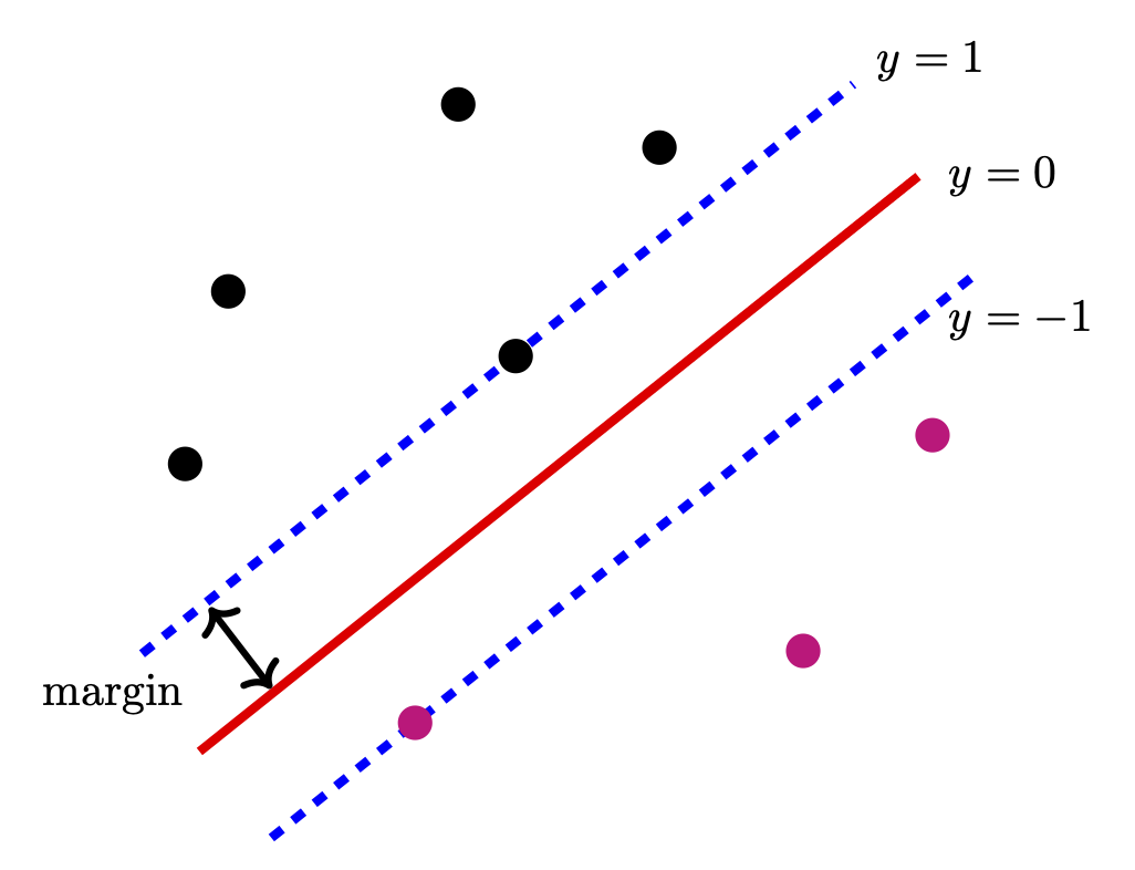
For convenience, we scale and such that the nearest points satisfy . This is called canonical scaling in the SVM literature and the expression is also called functional margin. Without loss of generality we can set this quantity to unity, since the direction of the hyperplane is unchanged when we scale both and by the same factor. The margin then becomes .
Maximizing is equivalent to minimizing :
| (302) | ||||
To solve the constrained optimization, we use the method of Lagrange multipliers, as described in Chapter 36. The Lagrangian becomes
where are the Lagrange multipliers.
Setting the partial derivatives of with respect to and to zero gives
Substituting these back into the Lagrangian yields the dual objective
| (303) | ||||
By the KKT Complementary Slackness condition (268),
This equation dictates exactly which points “exist” in the final model. To see this, note that based on this KKT condition, all training points fall into two mutually exclusive categories:
- 1.
Non-Binding Constraints (the “disappearing” points): If a point lies strictly outside the margin, then its margin is greater than 1, i.e.,
For the product in the KKT condition to be zero, the Lagrange multiplier must be
Looking at the formula for the weight vector,
(304) we see that these points make no contribution to the sum. If one were to remove these points from the dataset and retrain the model, the resulting hyperplane would remain identical. In the context of complementary slackness (cf. Chapter 36.3), we also refer to such data points as having “slack”.
- 2.
Binding Constraints (the support vectors): If a point lies exactly on the margin, then
In this case, the constraint is active, and can be non-zero (). These are the support vectors: they are the only points that “support” the hyperplane.
Let be the set of indices of the support vectors and denote the optimal weight vector by . We can rewrite the summation (304) as
Thus, is a linear combination of only the support vectors.
We summarize this insight in the following theorem:
Theorem 9.1 (Sparsity of the SVM).
The optimal weight vector of a Support Vector Machine is determined solely by the subset of training points for which the canonical functional margin is exactly .
Figure 52 illustrates SVM in action. Depicted are a linearly separable data set, the separating hyperplane computed by solving (302), the associated maximal margin and the support vectors.

41.2 Soft-margin SVM
In real-world data, classes often overlap. To accommodate a trade-off between the margin (the distance between the two critical hyperplanes) and the classification error on the training set, we introduce slack variables that allow points to be on the “wrong side” of the margin. Under this soft-margin constraint, the primal problem takes the form
| s.t. | |||
This is a convex quadratic program with linear constraints. Here, is a hyperparameter that controls the trade-off between maximizing the margin and minimizing classification errors. In the limit , we will recover the earlier hard-margin support vector machine.
The goal of the soft-margin SVM is to find a classifier that balances margin maximization and training errors, yielding robustness to noise and better generalization. Soft-margin SVM is also more robust to outliers, since it prevents a single anomalous data point from dictating the entire boundary.

It is instructive to rewrite the soft-margin SVM as an unconstrained optimization problem. To that end, we first express solely in terms of , and the data. From the constraints, we see that if the point is correctly classified and outside the margin (), the smallest possible that satisfies the constraints is . On the other hand, if the point violates the margin (), the smallest that satisfies the first constraint is . This can be written concisely as
By substituting the expression for back into the primal objective, we get
The term is known as the hinge loss. It is called “hinge” because of its shape: it is flat (zero) for values and increases linearly for values . As the hinge loss is an upper bound on the 0-1 indicator loss (misclassification count), minimizing the SVM objective provides a convex surrogate for minimizing classification error.
Logistic regression can also be considered as a variant of the SVM where the hinge function is replaced with the (smooth and convex) logistic function . Because the hinge loss is exactly zero for points far from the boundary, the gradient is also zero for those points. This is why SVMs are sparse (only support vectors matter). But unlike the logistic loss, the hinge loss is not differentiable at the “elbow” (where ). In practice, we use sub-gradient descent to solve this.
Figure 54 shows a comparison between logistic regression and soft-margin SVM. As we can see, the methods produce somewhat different decision boundaries. In logistic regression every point has a non-zero influence on the gradient because the sigmoid derivative is never exactly zero. In contrast, in SVM, once a point is correctly classified and beyond the margin, its gradient becomes exactly zero.

41.3 Kernel SVM
The SVMs we discussed so far are limited to datasets that are (approximately) linearly separable. However, for many real-world datasets this may not be the case. We can address this by mapping the input features into a higher-dimensional feature space via a non-linear mapping function with the aim that in this higher-dimensional space, a linear separation may become possible.
However, if we perform the mapping explicitly, we face a major computational challenge. Indeed, if we want to work in a high-dimensional space, the SVM dual objective requires us to compute the inner product of these transformed vectors. Thus, the kernel-analog of (303) takes the form
| (305) | ||||
In high dimensions calculating and then the inner product for every pair of points is computationally impossible.
The kernel trick introduced in Chapter 28, comes to our rescue: We can simply replace the inner product in (305) with the kernel function . We are now effectively computing the boundary in a high-dimensional space while only performing simple arithmetic in the original low-dimensional space. This modification of SVM is referred to as kernel SVM [77, 381]. The Gaussian kernel is a common default choice for kernel SVM.


42 Beyond binary classification
Binary classification addresses problems with only two possible outcomes. However, many practical and scientific applications naturally involve multiple classes, making multiclass classification essential. Indeed, in many domains, categories are inherently multi-valued, such as medical diagnosis with multiple disease categories, object recognition (car, pedestrian, bicycle,…), or document topic classification (politics, sports, technology,…).
42.1 Multiclass Logistic Regression (Softmax Regression)
While binary logistic regression uses the sigmoid function to map a score to a probability, multiclass logistic regression (also known as Softmax Regression) generalizes this by using the Softmax function.
For classes, we maintain separate weight vectors . For a given input , the probability that it belongs to class is
| (306) |
where the function on the right-hand side in (306) is also known as softmax function.
The denominator ensures that , creating a valid probability distribution. The optimization objective generalizes to the categorical cross-entropy loss
Here, the indicator is the “multiclass version” of the and used in binary logistic regression, which equals 1 if the true class of the -th sample is , and it equals 0 otherwise. is a matrix where each column (or row) corresponds to the weight vector for class . The decision rule consists of predicting the class with the highest probability: .
42.2 Multiclass Support Vector Machines
Unlike logistic regression, the SVM objective does not naturally produce a probability distribution across multiple classes. Instead, SVMs use meta-strategies to decompose the multiclass problem into multiple binary problems [229].
One such strategy is called “one-vs-all,” this is the most common approach. The strategy consists of training separate binary SVMs. For each class , we train a classifier where class is the positive label () and all other classes are the negative label (). For the prediction step we calculate the decision function for all classifiers. The input is assigned to the class with the highest (most positive) score. However, this approach comes with the drawback that the individual classifiers are trained on imbalanced datasets (one class vs. all other classes).
This issue can be mitigated by considering a “one-vs.-one” strategy. There, one trains a binary SVM for every possible pair of classes. This results in classifiers. The prediction is done via a “majority vote”: Each classifier performs a “vote.” If the SVM for class 1 vs. class 2 chooses class 1, then class 1 gets a point. The class with the most votes wins. This strategy has the benefit that each binary problem is smaller and more balanced, and it has the obvious downside that it is computationally more intense.
43 Rademacher complexity and generalization bounds
In this section, we develop a systematic connection between geometric measures of complexity and generalization guarantees for SVMs. We show how Rademacher complexity provides a natural measure that leads directly to margin-based risk bounds [54, 259, 386]. In a nutshell, Rademacher complexity is a measure of the richness of a class of (binary or real-valued) functions with respect to a probability distribution.
Let us start with a thought experiment6363 63 This thought experiment is inspired by lectures notes of Aditya Bhaskara on the Theory of Machine Learning, https://utah.instructure.com/courses/1023142.. Suppose there is an unknown distribution from which we draw i.i.d. samples . Let be a given loss function and let denote the associated empirical loss of a hypothesis , where denotes a (possibly infinite) hypothesis class6464 64 In statistical learning theory, a hypothesis class is the set of all prediction rules that a learning algorithm is allowed to choose from. For example, for linear classifiers, ., and its true (population) loss. We can compute , but since is usually unknown, we cannot calculate directly. In order to establish a generalization bound, we aim to show that the discrepancy between these two quantities is small uniformly over all .
To build intuition, consider the following experiment. Suppose we are given a fixed hypothesis together with the sample , and we wish to estimate the quantity . A natural approach is to employ a form of cross-validation: partition the sample into two disjoint subsets, (training) and (test), where for simplicity we assume that . We aim to approximate by
We now expand this expression more explicitly. Let be the indicator function that equals 1 if the hypothesis makes an error on the example , and equals otherwise. The expression above can therefore be rewritten as
| (307) |
Fixing the sample , each loss term appears with a coefficient of if and with a coefficient of if . Let us denote this sign by . With this notation, we may write
Now suppose the sample is fixed, and we form the partition into and uniformly at random. This is equivalent to choosing the signs independently and uniformly from , in which case the sum above can be viewed as a randomized estimate of the generalization gap. The resulting quantity is commonly referred to as a Rademacher average. Informally, Rademacher complexity, is the supremum of the quantity above, over .
We will make this concept now rigorous. We distinguish between the empirical version (calculated on a specific set) and the population version (an average over all possible sets) of Rademacher complexity.
Definition 9.2.
Let be a class of real-valued functions , and let be a fixed sample from . Let be independent Rademacher random variables, i.e.
The empirical Rademacher complexity of with respect to is defined as
Moving from this data-dependent estimate to its expected, distribution-level counterpart gives the population Rademacher complexity.
Definition 9.3.
Let be a distribution over . The (population) Rademacher complexity of with respect to samples from is
If , the same definitions apply verbatim, with .
Rademacher complexity is closely related to the Gaussian width, a concept arising in high-dimensional geometry and statistical learning theory which we will explore in depth in Chapter 58. For the current purposes, it suffices to know that for a closed set , the Gaussian width is defined as
Thus, for Rademacher complexity we are essentially replacing Gaussian random variables with Rademacher random variables. The close connection between these two concepts is further manifested by the following relationship between the Rademacher complexity and Gaussian width (see Exercise 9.3):
Rademacher complexity is one of the central tools in classical statistical learning theory. If a hypothesis class has low Rademacher complexity (or Gaussian width), it will generalize well, as established by the following theoretical analysis.
Definition 9.4.
Given a hypothesis , a loss function , and a training sample , the empirical risk is defined as
While the “true risk” (or “expected risk”) is the error we expect to see on all future, unseen data, the empirical risk is the error we can actually calculate using the data we have (the training set).
The following theorem connects the true risk to the empirical risk using the population Rademacher complexity. Intuitively, if a hypothesis class cannot fit random noise well, then empirical performance reliably predicts true performance.
Theorem 9.5 (Fundamental Generalization Bound).
Let be a hypothesis class of functions mapping to . For any , with probability at least over a sample of size , every satisfies
| (308) |
where is the expected risk, is the empirical risk on the sample , and is the population Rademacher complexity.
Proof.
The proof has three main components: (i) concentration, (ii) symmetrization, and (iii) reduction to Rademacher complexity.
(i) Concentration via McDiarmid’s Inequality: Define a function that represents the maximum gap between true and empirical risk for our class
We want to show that does not vary much if we change one element in . Let and differ only in the -th element ( vs ). We compute
where we have used that the range of is . By McDiarmid’s Inequality [307], with probability it holds that
| (309) |
(ii) Symmetrization: Now we bound the expectation
To that end, we introduce a “ghost sample” drawn from the same distribution. Note that . We have
where we have used Jensen’s inequality in the last step.
(iii) Introducing Rademacher variables: Since and are i.i.d., the distribution of is symmetric. We can multiply by Rademacher variables without changing the expectation and obtain
| (310) | ||||
where we have used the property of suprema (). Both terms are identical and equal to the population Rademacher complexity . Therefore, .
Substituting the result of (310) back into the McDiarmid bound from (309) gives
Since for all , the bound is proved.
∎
If we wish to use the empirical Rademacher complexity (which we can actually compute from data), the bound becomes slightly looser to account for the variance of the sample, namely
| (311) |
The proof of this bound is left to the reader (see Exercise 9.4).
We are now ready to state the Rademacher Complexity generalization bound for linear classes.
Theorem 9.6.
Denote and let be a sample such that for all . The empirical Rademacher complexity of satisfies
Proof.
We have
To maximize the inner product subject to the constraint , we choose to be in the same direction as the vector . Specifically, the optimal is . Substituting this in gives
| (312) | ||||
where we have used the concavity of the square root function and Jensen’s Inequality.
Furthermore,
| (313) |
Since the are independent and have mean zero we have that if , then , and if , then . Hence, the double sum collapses to .
Given our assumption that , we have . Substituting this back into the inequality (312) yields
∎
The following result, known as Talagrand’s Contraction Lemma, is the key tool for passing from linear predictors to hinge, logistic, or other Lipschitz losses in SVM analysis. It allows us to relate the complexity of the “composed” function class (loss hypothesis) back to the original hypothesis class.
Theorem 9.7 (Talagrand’s Contraction Lemma [278]).
Let be a class of functions mapping . Let be functions such that each is -Lipschitz. Then for any sample
Proof.
We assume without loss of generality. We proceed by induction on , the number of samples.
Let : We want to show that
Expanding the expectation gives
By the Lipschitz property we have . The right-hand side of the case is . We note that in our case, since and are interchangeable in the supremum, hence the inequality holds.
Assume now the theorem holds for . Let . We analyze
| (314) |
(where we have used the shorthand ) and isolate the expectation over . We get
For any fixed values of , let and be the functions that achieve the two suprema above. Then the expression inside the outer expectation is
| (315) |
Using the Lipschitz property, . We now consider the sign of : If , (315) becomes . If , (315) becomes .
In both cases, notice that this matches the expansion of the supremum of the untransformed -th variable
Substituting this back into (314) gives
By repeating this argument for , we peel away each one by one. After iterations, we obtain
This completes the proof.
∎
It is easy to see that the hinge loss and the logistic loss are 1-Lipschitz. Therefore, by virtue of Talagrand’s Contraction Lemma, generalization bounds for linear predictors automatically extend to SVM and logistic regression, as manifested by the Theorem 9.8 below.
We define the margin loss (or ramp loss) by
Theorem 9.8.
Let be a distribution over , where is an input space such that for all . Let denote the hypothesis class defined by
For any margin , and for any , with probability at least over the choice of a sample drawn i.i.d. from , every satisfies
Proof.
We want to bound the true risk . Define the indicator loss . The margin loss function is defined such that for all
Therefore, the true risk is dominated by the expected margin loss
Let be the family of functions . Since the range of is , we apply the bound (311). For any , with probability at least
| (316) |
Note that is -Lipschitz with . By Talagrand’s Contraction Lemma,
| (317) |
Consider the term . Since are fixed constants in the empirical complexity and are independent Rademacher variables, the product is also a Rademacher variable with the same distribution as . Thus,
where we have used Theorem 9.6 in the last step. We combine this bound with the inequality (317) and obtain
| (318) |
Substitute the bound from (318) into the generalization inequality (316) gives
We complete the proof by noting that .
∎
When applying standard SVM, we assume the data is (essentially) linearly separable. Assuming the linear separability holds strictly, then in hard-margin SVM the optimization ensures that for all training points, . If we set our theoretical margin parameter , then the hard-margin SVM ensures , which means for every single training point. Therefore, the empirical risk term in Theorem 9.8 becomes zero. The generalization bound then tells us that the true error is entirely bounded by the complexity term and the concentration term.
In a soft-margin SVM, we allow some points to violate the margin using slack variables . Recall that the hinge loss, , is an upper bound on the ramp loss . While the ramp loss is what we use in the theorem to get a tight bound between 0 and 1, the soft-margin SVM actually minimizes the hinge loss because it is convex and easier to solve via quadratic programming. Because , minimizing the hinge loss is a principled approach to trying to minimize the empirical term in the margin generalization bound.
The generalization bounds are also applicable to kernel-SVM. It is not difficult to establish the following result (see also Exercise 9.5).
Theorem 9.9.
Let be a symmetric, positive-definite kernel, and let be its associated Reproducing Kernel Hilbert Space with norm . Assume there exists a constant such that for all . Let
Then with probability at least
In this RKHS setting, the empirical Rademacher complexity is strictly bounded by the trace of the kernel matrix
Thus, Theorem 9.9 shows that even if is infinite-dimensional (like with a Gaussian kernel), the complexity of the learning task is governed only by the norm of the function (the parameter ) and the kernel’s behavior on the data (the parameter ), not the dimensionality of the space.
44 Alternative classification methods
The choice of classification method depends strongly on factors like the inherent structure of the data (such as its dimensionality, sparsity, and linearity), the practical setting (for instance, a high-frequency trading platform might prioritize speed, while in medical diagnostics accuracy or need for interpretability may have higher priority), the available computational resources, as well as the amount of labeled data available and the signal-to-noise ratio.
Thus, the optimal classifier is not necessarily the most complex one, but rather the model that best balances accuracy, interpretability, robustness, and feasibility within the constraints of the intended application. With this in mind, we briefly mention a variety of alternative classification methods beyond linear models and margin-based classifiers which are widely used in practice.
-Nearest Neighbor (k-NN) methods [129] classify data points based on local proximity in feature space and require minimal modeling assumptions, although they scale poorly with dimension.
Random Forests and related tree-based ensembles [222, 80] construct classifiers by aggregating many randomized decision trees, offering strong empirical performance and robustness at the cost of reduced interpretability.
Boosting methods, such as AdaBoost and gradient boosting [176, 177, 114], combine weak learners into a powerful classifier through iterative reweighting, with strong theoretical guarantees under suitable conditions.
Neural networks are currently the state-of-the-art approach for multiclass classification, particularly when the relationship between the input features and the classes is non-linear or highly complex (like in images, audio, or natural language) and when a large number of training data is available.
In fact, the multiclass logistic regression model can be interpreted as a “single-layer” neural network. Deep Learning expands this by adding hidden layers between the input and the final softmax output. We will explore neural networks in more detail in Chapter 10.
Exercises
Exercise 9.1.
(a) Write down the KKT conditions for the soft-margin SVM.
(b) Interpret each KKT condition geometrically.
(c) Explain how complementary slackness characterizes support vectors.
Exercise 9.2.
Generate a binary classification dataset in via:
-
Class : 100 samples from ,
-
Class : 100 samples from .
(a) Fit logistic regression with no regularization;
(b) Fit logistic regression with -regularization .
Compare norm of the weight vector, classification accuracy, and margin width. Visualize decision boundaries.
Exercise 9.3.
Show that the following relationship between the Rademacher complexity and Gaussian width holds:
Exercise 9.4.
Prove the following data-dependent generalization bound:
For a hypothesis class mapping to , with probability at least over a sample of size , every satisfies
Exercise 9.5.
Prove Theorem 9.9.
Exercise 9.6.
Consider a soft-margin SVM where each training example is a triplet with denoting the importance of example .
- (a)
Modify the primal optimization problem so that the penalty for violating the margin constraint on example is scaled by .
- (b)
Derive the corresponding dual optimization problem and describe how the importance weights affect the dual variables.
- (c)
Briefly interpret the effect of on the solution.
Exercise 9.7.
Suppose we have a binary classification problem in one dimension. The two classes, and , are distributed according to Gaussian probability density functions:
- (i)
Class 0 (Negative): ,
- (ii)
Class 1 (Positive): .
Assume and that the classes have equal prior probabilities, . We define a classifier with a decision threshold (cut-off) , such that we predict class if , and class otherwise.
Derive analytical expressions for the following metrics as a function of the threshold , the means , and the variance . Use the standard normal cumulative distribution function or the complementary error function in your answers.
- 1.
True Positive Rate (Sensitivity): .
- 2.
True Negative Rate (Specificity): .
- 3.
False Positive Rate: .
- 4.
The Confusion Matrix: Express the expected values of the matrix entries for a dataset of size .
- 5.
ROC Curve Equation: Derive the functional relationship between TPR and FPR by eliminating .
- 6.
Area Under the Curve: Show that the AUC for this 1-D Gaussian case is given by .
Exercise 9.8.
The MNIST dataset consists of grayscale images of handwritten digits , each represented as a vector in . In this problem, we consider the binary classification task of distinguishing between the digits 3 and 8. Let
denote the dataset, where corresponds to the digit 8 and corresponds to the digit 3.
Extract all images of digits 3 and 8 from the MNIST dataset, and normalize each image so that its pixel values lie in . Split the data into a training set and a test set .
(a) Compare logistic regression and soft-margin SVM in terms of classification accuracy, convergence behavior, and robustness to misclassified samples.
(b) Visualize several test images that are misclassified by each method.
Exercise 9.9.
(The Breast Cancer Wisconsin Diagnostic Dataset).
Download the Breast Cancer Wisconsin (Diagnostic) dataset (e.g. from the UCI Machine Learning Repository). The goal in this exercise is to predict whether a tumor is malignant or benign based on 30 features (radius, texture, smoothness, etc.).
(a) Train SVM on the raw data. Then, standardize the features (subtract mean, divide by standard deviation) and retrain. Why does the SVM performance change so drastically with scaling, while Logistic Regression is relatively more robust?
(b) Extract the weights from the Logistic Regression model. Which physical feature (e.g., “area” vs. “concavity”) is the strongest predictor of malignancy?
Exercise 9.10.
The Spambase dataset (UCI Machine Learning Repository) consists of email messages represented as feature vectors of 57 attributes. Each email is labeled as either spam or non-spam. Let
denote the dataset, where corresponds to spam and corresponds to non-spam.
(a) Train logistic regression models for -regularization, -regularization, and
no regularization.
(b) Train a soft-margin SVM.
Compare logistic regression and soft-margin SVM in terms of classification accuracy, sparsity of learned parameters, and robustness to regularization parameter choice.
Exercise 9.11.
The goal of this exercise is to compare the performance of Support Vector Machines and Feed-Forward Neural Networks as a function of training set size. This project consists of four parts.
Load the MNIST Dataset: Filter the dataset to include only the two digits 4 and 9. This pair is chosen because these two digits are visually (somewhat) similar and provide a meaningful challenge. Flatten the images into 784-dimensional vectors. Scale the pixel values to the range . Reserve a fixed test set of 1,000 images for evaluation.
You will train two models:
- •
Model A (SVM): Use a Gaussian kernel with and .
- •
Model B (Neural Network): A simple Multi-Layer Perceptron (MLP) with one hidden layer of 100 neurons, using ReLU activation and a Sigmoid output layer. Use the Adam optimizer with a learning rate of .
Train both models on subsets of increasing size of the training data: for each subset size , record the test accuracy. (To ensure statistical stability, you should repeat each training session five times with different random subsets and report the average accuracy.)
- (a)
At what value of (roughly) does the neural network begin to outperform the SVM? Explain why the SVM performs better at very low values of .
- (b)
Overfitting: Compare the training accuracy vs. test accuracy for the neural network at . What does this gap tell you about the model’s complexity relative to the data size?
- (c)
Support Vectors: For the SVM model, calculate the number of support vectors. How does this number compare to the total number of parameters in your neural network?
Exercise 9.12.
This exercise deals with a highly imbalanced dataset, a problem we often encounter in practice.
From the MNIST dataset select two classes: Pick digit “0” (Majority) and digit “8” (Minority). Create an imbalanced dataset by taking 5,000 samples of the digit “0”, and taking only 50 samples of the digit “8”. Combine them into a training set where the minority class represents only 1% of the data. But use a balanced test set (500 of each) to see how the model generalizes. Train a baseline by training a standard Logistic Regression or SVM on this imbalanced set. Then calculate accuracy: You will likely achieve 99% accuracy (why?) Calculate the Precision, Recall, and F1-Score. If the model simply predicts “0” for every single image, what would the accuracy be? Is this model actually useful?
We will explore different intervention strategies to address this imbalance problem.
- 1.
Class weighting: Modify the SVM or Logistic Regression loss function to penalize mistakes on the minority class more heavily.
- 2.
Precision-recall thresholding: Instead of using the default 0.5 probability threshold, move the decision boundary. Plot a Precision-Recall Curve. Find the threshold that yields a Recall of at least 0.80 and report the resulting Precision. The ROC Curve and the Precision-Recall Curve are both used to evaluate classifiers. In this imbalanced experiment, which curve was more “honest” about the model’s poor performance on the minority class? Why?
- 3.
Data augmentation: Come up with your own strategy to create additional (synthetic) versions of the digit “8”. But you can only use the current 50 digits of “8” to do this, you cannot simply add other digits “8” from the MNIST dataset or some other existing dataset.
- 4.
Subsampling: Create a balanced dataset by downsampling the majority class to 50 samples.
Compare the results of the three different strategies to the baseline in terms of accuracy, precision for digit “8”, precision for digit “0”, and F1-score. Comment on the advantages and disadvantages of each strategy. Which intervention strategy seems most promising?
Chapter 10 A Mathematical Introduction to Deep Learning
Deep learning has emerged as one of the most intriguing developments in modern data science, offering a powerful framework for learning complex patterns directly from data. Unlike traditional machine learning methods that rely heavily on feature engineering, deep neural networks automatically extract hierarchical representations that capture both low-level and high-level structures in data. This capability makes deep learning particularly effective for classification tasks, where the goal is to assign inputs—such as images, sounds, or text—to discrete categories. By composing multiple layers of nonlinear transformations, deep learning models can approximate highly intricate decision boundaries, often achieving impressive performance across a wide range of domains.
The 2024 Nobel Prize in Physics and the 2024 Nobel Prize in Chemistry marked a significant moment of recognition for the field of deep learning and its far-reaching scientific impact. Together, these awards signal how deep-learning architectures have moved from niche algorithmic innovation to being recognized as powerful scientific tools.
Despite this phenomenal empirical success and scientific recognition, the field’s underlying mathematical theory is still nascent; many fundamental questions regarding optimization, generalization bounds, and the precise reasons for the efficacy of overparameterized models remain open problems at the intersection of mathematics, statistics, and computer science.
At its core, deep learning leverages artificial neural networks with many layers—hence the term “deep”—to model complex relationships in data. This chapter provides a mathematical perspective on deep learning, focusing on the foundational concepts and structures that underpin the field. Deep learning has developed its own jargon, often coming up with new names for already well established procedures in signal and image processing, optimization, or statistics. We follow in part the very accessible article by Higham and Higham [218] when bridging deep learning and applied mathematics. We also recommend [353] which covers several topics that we do not discuss in this chapter, such as the generalization properties of deep neural networks.
45 Neural networks
Neural networks are a cornerstone of modern artificial intelligence, capable of learning patterns from data. Neural networks are used in a variety of applications, including image recognition, natural language processing, and even playing complex games like Go and Chess. Here we focus on using neural networks for classification.
Suppose we have a training dataset of points in consisting of two classes and , drawn from some underlying distribution of data with the same labels. Based on this training set, we are looking to design a function that will generate labels for new data, for example, the black question mark in Figure 56
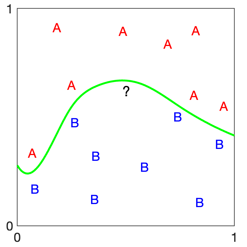
If the green line represents the decision boundary of , then the question mark will be classified as a . Artificial neural networks (or neural networks for short) are a way of generating this function .
45.1 Perceptrons
A neural network is composed of layers of neurons, where each neuron (or node) is a computational unit that processes input and produces an output. The perceptron, introduced by Frank Rosenblatt in 1958 [374], is one of the simplest models of a neuron. Mathematically, a perceptron can be described as:
where are the input features, are the weights associated with the inputs, is the so-called bias term, is an activation function (typically a Heaviside step function, but more generally it can be a nonlinear function like the sigmoid).
A multilayer perceptron (MLP) extends the perceptron by stacking multiple layers of nodes. An MLP consists of an input layer, one or more hidden layers, and an output layer. Each layer in an MLP is described by the following equation:
where is the output of the previous layer (or the input data for the first layer), is the weight matrix for layer , is the bias vector for layer , and is an element-wise activation function. An MLP is a specific type of neural network, more specifically a subclass of feedforward neural networks. More generally, neural network is an umbrella term that includes various architectures beyond just feedforward networks.
To introduce some further standard terminology, the first layer of a neural network is called the input layer, which usually just corresponds to the data. A hidden layer in a neural network is any layer of nodes that is situated between the first layer and the last layer. The term “hidden” refers to the fact that these layers are not directly exposed to the input data or the final output; they are “hidden” in the sense that they exist only within the network’s architecture. The last layer is the output layer, typically associated with a loss function that measures the discrepancy between the predicted output and the true output. The output layer shapes the data into a shape more appropriate for the downstream task. For example the output layer may transform the data from a hidden shape of, say, 1024, to a shape of 2 for a binary prediction.
45.2 General setup
We assume the following general setup: The network has layers, with layers and being the input and output layers, respectively. We assume that the number of nodes in the -th layer is , for . Thus the input dimension is and the output dimension is . We denote the matrix of weights at layer by , where is the weight that node at layer applies to the output from node at layer . Similarly, is the vector of biases for layer . Hence, the bias is associated with node at layer .

A neural network with four layers is illustrated in Figure 57 (for simplicity the bias terms are omitted in that figure). represents the connection between unit in layer and unit in layer , so the rows of correspond to the weights going into node . In this spirit, we define to be the row vector of . In the example shown in Figure 57, , , and . Also, denotes the output, or activation, of unit in layer , while is the sum into node . Hence, in the above example:
We can now represent the action of a deep neural network with layers in the following form: Given an input , let denote the output, or activation, from neuron at layer . We compute:
| (319) |
where, the activation functions and the number of nodes may differ from layer to layer.
Suppose now that we are given a set of data points (our training set), for which we have associated target outputs . The might be images, each showing either a car or a bicycle, and the corresponding might be binary labels indicating class membership, i.e., if the depicted object in image is in fact a car or a bicycle. The task of training a neural net is to minimize a user-specified cost function or loss function which takes as input and which will depend on all the weights and biases . One example of such a cost function is
We will discuss other choices of loss functions and how such a network is typically trained (i.e, how to find the weights and biases that minimize the loss function) in Section 47.
45.3 Activation functions
The activation function introduces non-linearity into the model, with the intention that it should enable the network (assuming sufficiently many nodes and layers) to learn complex patterns. We briefly discuss some common activation functions. Sigmoidal type functions satisfy the properties and . The sigmoid or logistic function
an example of a sigmoid function, maps the input to a value between 0 and 1, making it useful for binary classification problems, as we already have seen in Chapter 9. The hyperbolic tangent
maps the input to a value between -1 and 1, and it is often used in hidden layers of a neural network. The Rectified Linear Unit (ReLU)
is the most popular activation function in deep learning. It is computationally efficient and helps mitigate the vanishing gradient problem [224, 66]. However, it is not differentiable at the origin. The softmax function:
| (320) |
is typically used in the output layer of a network for multi-class classification problems. It converts the raw output scores into probabilities.


Which activation function shall we use in which layer? Except for the last layer, where the activation function is in part determined by the task at hand (e.g. a classification task will suggest something like a softmax activation function while a ReLU would not help in that case), choosing an activation function is done mainly via trial and error.
While trial and error is often good enough for most application, one might ask if, instead of such an ad hoc approach, can we take a data driven approach and learn the activation functions like we do for the weights and biases? One approach to do this in a principled manner is given by Kolmogorov-Arnold Networks which have learnable activation functions. Indeed, Kolmogorov-Arnold Networks have no linear weights at all, since every weight parameter is replaced by a univariate function parametrized as a spline. We refer to interested reader to [293] for details.
46 The Universal Approximation Theorem
Although many facets of deep learning still lack a thorough mathematical explanation, the approximation properties of (shallow) neural networks are relatively well understood. The Universal Approximation Theorem [227, 228, 132, 354, 53] is a fundamental result in neural network theory. It essentially states that a feedforward neural network with a single hidden layer containing a finite number of nodes can approximate any continuous function on compact subsets of , given appropriate parameters (weights and biases).
46.1 A “shallow” theorem
One of the foundational versions of the Universal Approximation Theorem (UAT) for shallow neural networks is due to George Cybenko [132]. It applies to single-hidden-layer feedforward networks with sigmoidal activation functions. We need some notation before we can present the rigorous statement.
Let be the unit hypercube in , and let be the space of continuous real-valued functions on , equipped with the supremum norm . We recall that a function is called sigmoidal if and .
Theorem 10.1 (Cybenko, 1989).
: Let be any continuous sigmoidal function. Then, the set of all finite sums of the form
where , , and , is dense in . In other words, for any and any , there exists such a satisfying
This theorem implies that a single-hidden-layer neural network with a continuous sigmoidal activation function (e.g., the logistic sigmoid ) can approximate any continuous function on a compact set to arbitrary accuracy, provided sufficiently many hidden neurons are used. Note that the result extends naturally to any compact subset of by rescaling and shifting, and to multi-output functions component-wise.
The proof relies on concepts from functional analysis, including the Hahn-Banach theorem and the Riesz representation theorem. It first establishes a more general result for “discriminatory” functions defined below, and then shows that continuous sigmoidal functions are discriminatory.
Definition 10.2.
Let denote the space of finite signed regular Borel measures on . A function is called discriminatory if, for any ,
implies .
Theorem 10.3.
Let be any continuous discriminatory function. Then, finite sums of the form
are dense in .
Proof.
Let be the subspace of consisting of all finite linear combinations of functions of the form for and (i.e., the span of such functions). Clearly, is a linear subspace.
Assume, for contradiction, that the closure (in the supremum norm) is a proper closed subspace of . By the Hahn-Banach theorem, there exists a nonzero bounded linear functional such that for all (and hence for all ).
By the Riesz representation theorem, since is a bounded linear functional on , there exists a unique such that
In particular, for each fixed and , the function belongs to (and thus to ), so
Since is discriminatory, this implies . But means , contradicting the assumption that .
Therefore, , so is dense in . ∎
To apply Theorem 10.3 to sigmoidal functions, we need the following result:
Lemma 10.4.
Any continuous sigmoidal function is discriminatory.
Proof.
Assume
We aim to show that .
Fix , , and consider scaling the argument. For any , replace with and with :
As , the integrand converges pointwise to the step function
(since is sigmoidal with limits 1 and 0). Moreover, since is continuous and thus bounded on , the convergence is bounded.
By the Lebesgue dominated convergence theorem (applicable because has finite Lebesgue measure and the functions are bounded),
where is the open half-space and is the hyperplane.
To isolate terms, note that by varying slightly or using different scalings, we can show for almost all hyperplanes (since hyperplanes have measure zero in general position). More rigorously, consider the pushforward measure along the line in direction .
Define the linear functional by
which is well-defined and bounded (since is finite). The assumption implies for all , and by the scaling argument above, vanishes on the indicators of half-lines for any (by choosing appropriate ).
Since indicators of intervals generate the Borel algebra, and simple functions (finite linear combinations of indicators) are dense in for the induced measure (the pushforward of under the map ), vanishes on a dense set in the continuous functions.
In fact, since for the Fourier basis (by approximating exponentials via sigmoidal superpositions or directly from the vanishing on steps), the characteristic function of the pushforward measure is zero everywhere, implying the pushforward is zero. Thus,
implying the Fourier transform of vanishes, so by uniqueness of Fourier transforms for measures. ∎
of Theorem 10.1.
This proof demonstrates the validity of Theorem 10.1 without constructing explicit approximations, relying instead on separation theorems in functional analysis. Extensions (e.g., [227, 228]) provide alternative proofs for broader classes of activations, see also [353].
However, since the proof is nonconstructive, it “only” guarantees the existence of an approximating neural network, but it does not provide a method to find the weights or the number of neurons .
There exists extensive theory establishing convergence rates for the approximation of a function by a neural network, see e.g. [311, 354, 143]. For classical smoothness spaces it has been shown that to achieve an accuracy of , the size of the network needs to increase exponentially in , and this exponential dependence on is unavoidable [344, 143].
Thus, additional assumptions on the function are needed if one wants to avoid this curse of dimensionality. One such regularity assumption is captured by the so-called Barron class. Barron, in [53], introduces a Banach space of regular functions (now known as Barron class), defined by the semi-norm . Barron shows that, for any , there exists a network with neurons such that the approximation error is of the order , when measured in the -norm.
46.2 When is deep better than shallow?
Adding more layers (depth) does not increase the class of functions that can be approximated in principle, since we just saw that even one hidden layer already suffices for density. But it dramatically changes the efficiency and representational complexity of approximation.
It is known (see e.g. [356, 467, 414]) that some functions can be approximated exponentially more efficiently by deep networks than by shallow ones. For example let be a high-order monomial. In this case it has been shown that a shallow network needs exponentially many neurons in to approximate , while a deep network can approximate with neurons using compositional structure [356].
However, while it is not too difficult to construct a neural network (deep or shallow) that enables some form of universal approximation power, it is important to emphasize that this sheds little light on the success of deep learning. How come (carefully fine-tuned) neural networks with a huge number of parameters (weights) are able to generalize astonishingly well? Traditional approaches fail to explain why large neural networks generalize well in practice [471, 472].
Can Rademacher complexity help? Recall that Rademacher complexity bounds measure the worst-case capacity of an entire hypothesis class, and for large neural networks these bounds are often huge, leading to vacuous generalization bounds. However, the effective complexity seems to be much smaller than the worst-case class complexity. Understanding precisely when and why overparameterized networks generalize remains one of the central open questions in modern learning theory.
The “double descent phenomenon” is a noteworthy theoretical development in this context, which helps to shed some light on why deep neural networks generalize so well despite being massively overparameterized [56]. It suggests that in the highly over-parameterized regime, deep networks achieve generalization by finding the most mathematically parsimonious way to interpolate the training data. Thus, the double descent curve refines our understanding of the bias-variance tradeoff in the overparametrized regime. Generalization depends not just on model size, but how the model is trained and which solutions are preferred.
46.3 Infinite depth: Neural differential equations
When we let the depth of a neural network approach infinity, we arrive at so-called neural differential equations [113]. To see this, let us consider a standard feedforward neural network with layers, where each layer applies a transformation of the form
with denoting the input and the final hidden representation or output. This formulation corresponds to a residual network (ResNet) architecture, in which the update rule explicitly adds a residual term to the identity mapping.
To interpret this recursion as a discretization scheme, introduce a continuous “depth” variable and let each layer correspond to a discrete time point with step size . Then the layer-wise update can be rewritten as
This is precisely the forward (explicit) Euler method applied to the initial value problem
Hence, in the limit as the number of layers (and thus , the discrete-depth neural network converges formally to a neural differential equation, or more specifically, a neural ordinary differential equation. The dynamics of the hidden representation are governed by
where is a neural network parameterizing the instantaneous rate of change of .
This continuous-depth perspective allows one to treat neural network architectures as parameterized dynamical systems. The terminal state is obtained by integrating the differential equation from to ,
and the parameters are optimized to minimize a loss functional defined over the final state.
From an analytical viewpoint, this interpretation reveals that the expressiveness of deep networks can be understood through the lens of continuous-time dynamical systems theory, with residual connections corresponding to first-order numerical integration schemes.
47 Training neural networks
Training a neural network involves finding the optimal weights and biases that minimize a cost function or loss function . Due to the typically large amount of data, higher-order optimization methods are usually prohibitively expensive. The work horse for this process typically comprises gradient-based optimization algorithms, regardless of the specific network architecture.
47.1 Loss functions
Loss functions (called cost functions in optimization or error functions in numerical analysis) are critical in guiding the learning process by quantifying how well the model’s predictions align with the true targets. The choice of the loss function depends on the specific task (e.g., regression, classification) and the characteristics of the data. For example, the mean squared error is often employed for regression tasks:
The mean absolute error is given by
It is also used for regression tasks, particularly when robustness to outliers is desired, since it is less sensitive to outliers than the mean squared error.
The cross-entropy loss is a standard choice for classification tasks:
The multi-class cross-entropy loss generalizes binary cross-entropy to multiple classes. In detail, for multi-class classification, where the true target is a one-hot encoded vector and the predicted probabilities for each class are given by , the cross-entropy loss is:
where is the number of classes, is the true label (1 or 0) for class , and is the predicted probability for class .
The Hinge Loss is primarily used in Support Vector Machines but also finds use in neural networks. For binary classification, where and is the predicted score (not a probability), the hinge loss is defined as:
The hinge loss is used in contexts where the predictions are scores rather than probabilities, and it aims to ensure that the true class is not only predicted correctly but with a margin of at least 1. If , the loss is 0, meaning the prediction is correct with a sufficient margin. If , the loss increases linearly, penalizing the model for incorrect or insufficiently confident predictions.
The Kullback-Leibler (KL) Divergence measures how one probability distribution diverges from a second, expected probability distribution. It is typically used in variational autoencoders and reinforcement learning. For two probability distributions (true distribution) and (predicted distribution), the KL divergence is defined as:
It is not symmetric, meaning . In deep learning, the KL divergence is often used in settings where the model needs to match its output distribution to a target distribution .
The Huber loss attempts to combine the best properties of the mean squared error and the mean absolute error. For a prediction and target , it is defined as:
where
The Huber loss is typically used for regression tasks, particularly when dealing with outliers. It is less sensitive to outliers than the mean squared error.
47.2 Stochastic gradient descent
Training a neural network corresponds to choosing its parameters, i.e., the weights and biases, that minimize the cost function. Given the high dimensionality and non-linearity of neural networks, finding the optimal parameters becomes a challenging task. So, how shall we do that?
Enter gradient descent ! The use of gradient descent is usually discouraged in classical numerical optimization and often for good reason: Gradient descent generally can have a slow rate of convergence, is sensible to the choice of step size and initialization, and can easily get stuck in saddle points and local extrema [343]. However, in many applications in data science and machine learning it suffices to compute a solution with relatively low accuracy and often one is content with finding local minima. Also, since gradient descent uses only first-order information (namely, the gradient), it can better cope with limited computing resources vis-à-vis very large datasets compared to second-order methods. Due to these considerations gradient descent has become the workhorse in training neural networks.
Specializing the results in Chapter 37 to the setting to neural networks, we interpret as the network’s cost function , with its parameters (the weights and biases) collected in the vector .
Deep learning uses stochastic gradient descent (SGD), which was discussed in Chapter 37, instead of standard (full-batch) gradient descent because of computational, statistical, and optimization-landscape reasons that become decisive at the scale and structure of modern neural networks.
Recall that in the standard gradient descent algorithm, the gradient is computed as
where represents the loss for the -th data point.
In contrast, SGD updates the parameters using the gradient computed from a single randomly selected data point :
A common variant of SGD in deep learning is mini-batch gradient descent, where the gradient is computed over a small batch of data points instead of a single data point
where is the set of indices in the -th mini-batch, and is the batch size. Mini-batch gradient descent attempts to strike a balance between the computational efficiency of SGD and the stability of full-batch gradient descent. It is widely used in practice due to its ability to leverage parallelism and its effectiveness in noisy environments. The convergence of SGD can be analyzed in terms of the expected value of the loss function, see also Section 37.7.1 for the special case of applying SGD to a linear system of equations.
The step size of gradient descent, in this context called the learning rate, is an important design parameter. If the learning rate is too large, the noise can cause the algorithm to diverge. Conversely, if the learning rate is very small, the algorithm may converge rather slowly. If the learning rate is sufficiently small, SGD converges to a neighborhood around a local minimum. The exact nature of this neighborhood depends on the noise characteristics and the curvature of the loss function.
One way to enhance stability is to use a decaying learning rate
where is the initial learning rate, and is a decay factor.
Adaptive methods such as Adam [253] or AdaGrad [160] adjust step sizes dynamically and this frequently leads to empirical improvements but complicates the theoretical guarantees [454]. While Adam is often the method of choice for training speed, it has been observed in simulations that switching to SGD with momentum (see Chapter 37 for a discussion of gradient descent with momentum) for the final stages of training can achieve better generalization on test data for some architectures [460].
47.3 Backpropagation
Backpropagation is the fundamental algorithm used for training neural networks by computing the gradients of the loss function with respect to each weight in the network. It leverages the chain rule from calculus to efficiently compute the gradient of the loss function with respect to every weight in the network.
It will be convenient in the following to denote a neural network by a function , where are the input data and represents all the weight and bias parameters. The goal of training is to find the set of parameters that minimizes a loss function . It will be helpful in our derivation of the backpropagation algorithm to make the dependence of the loss function on the the network parameters explicit by writing . We are concerned with solving:
where, as above, is the true output for input . Backpropagation computes the gradient so that the weights can be updated using (stochastic) gradient descent:
where is the learning rate.
The goal is to compute and for all weights and biases . The input to neuron in layer is a weighted sum of the outputs from the previous layer, , i.e.,
Applying the chain rule, the gradient of the loss with respect to a weight in layer is:
From the definition of , we have
Substituting this back, and defining the term
the weight gradient becomes
| (321) |
Similarly, the bias gradient is
| (322) |
The key challenge is to compute the error term for all layers. The loss depends directly on the output activations and the activations depend on the net inputs . We have
Since , the second term is the derivative of the activation function
Hence, the output layer error is
| (323) |
The error term for a hidden layer is found by relating it to the errors in the next layer, . This is where the name backpropagation comes from.
Applying the chain rule again gives
| (324) |
where the sum is over all neurons in layer .
Substituting the definition into (324) yields
| (325) |
Now we compute the second term. From and we get
Plugging this back into equation (325) gives
We now factor out the term which is independent of the summation and arrive at
| (326) |
This is the “Backpropagation Error Equation”: the error at layer is calculated by taking a weighted sum of the errors from the next layer and multiplying it by the derivative of the activation function at layer .
Backpropagation has two phases, a forward pass and a backward pass. The forward pass consists of the following steps:
- 1.
Initialize all weights and biases .
- 2.
Propagate the input through the network, layer by layer, computing all net inputs and activations for all .
- 3.
Compute the loss at the output layer .
The backward pass consists of four steps which comprise the gradient calculation and update:
- 1.
Output error (): Compute the error term for the output layer using equation (323):
- 2.
Backpropagate error (): Compute the error term for each preceding layer using the errors from the layer above (equation (326)):
- 3.
- 4.
Update parameters: Perform a gradient descent step to update the weights and biases
Backpropagation is computationally efficient because it reuses intermediate computations from the forward pass. Specifically, it computes gradients layer by layer in reverse, leveraging the fact that the gradient of the loss with respect to earlier layers can be expressed recursively in terms of gradients from later layers. This efficiency is crucial for training deep neural networks, where the number of parameters can be large, and the computation of gradients must be optimized.
47.4 Regularization
Training deep networks presents several challenges, which necessitate the use of some form of regularization. These challenges include:
Vanishing and exploding gradients: During backpropagation, gradients can become very small or very large, making learning difficult. Techniques such as careful initialization, batch normalization, and gradient clipping as well as using ReLU as activation function are used to mitigate these issues.
Overfitting: Deep networks with many parameters are prone to overfitting the training data. To prevent overfitting, regularization techniques are often employed. Common methods include adding a penalty term such as to the loss function and a technique called dropout: to randomly drop units from the neural network during training to prevent co-adaptation of neurons.
Early stopping is a particularly effective strategy in which training is halted once performance on the validation set ceases to improve. This implicitly regularizes the model and reduces the risk of fitting noise in the training data.
Data augmentation is another technique used to avoid overfitting by increasing the diversity of the training data without actually collecting new data. It involves applying various transformations to the existing data to create new, slightly modified versions of it. For example, in image classification, an object should be recognizable regardless of its position, orientation, or lighting conditions. By augmenting the data to include controlled variations in the image training data, such as shifts, rotations, flips, scaling, and changes in brightness or contrast, we can help the model to generalize better to unseen data.
47.5 Practical setup for training neural networks
Training a neural network is not only a matter of choosing an architecture and an optimization algorithm; it also requires a carefully designed experimental protocol to ensure that the resulting model generalizes beyond the data it was trained on. We briefly describe best practices for setting up a reliable neural network training pipeline. These principles actually apply to any supervised data science learning task.
A fundamental principle of supervised learning is the separation of data into disjoint subsets with distinct roles. Typically, the available dataset is divided into a training set, a validation set, and a test set. A common heuristic is to split the data into 70% training, 10% validation, and 20% test data6565 65 While an 70-10-20 split is a typical starting point for medium-sized datasets, in the era of “Big Data” , it is not unusual to see 98-1-1 splits, as even 1% of data can provide a statistically significant evaluation. Nevertheless, a more conservative split provides a better defense.
The training set is used to fit the model parameters via optimization algorithms such as stochastic gradient descent. The validation set is used to tune hyperparameters and make modeling decisions, while the test set is held out and used only once to obtain an unbiased estimate of the final model’s generalization performance. Cross-validation (introduced in connection with ridge regression in Definition 4.15) is typically used for parameter tuning. Crucially, the test set must not influence any aspect of model design or training.
Neural networks involve numerous hyperparameters, including learning rates, batch sizes, network depth and width, regularization coefficients, and optimization settings. Hyperparameter tuning is typically performed by training multiple models on the training set and evaluating their performance on the validation set. Techniques range from manual tuning and grid search to more sophisticated approaches such as random search or Bayesian optimization. Importantly, all hyperparameter choices must be finalized before evaluating performance on the test set.
Data leakage occurs when information from outside the training set is inadvertently used during training or model selection, leading to overly optimistic performance estimates. Common sources of leakage include preprocessing steps (such as normalization or feature selection) performed using the full dataset, or repeated evaluation on the test set during model development.
To avoid data leakage, all data-dependent preprocessing operations should be fit exclusively on the training data and then applied unchanged to the validation and test sets. Likewise, the test set should remain completely isolated until the very end of the training pipeline.
Once the training and tuning process is complete, the final model is evaluated on the test set to estimate its generalization performance. This evaluation should be performed exactly once to prevent data leakage.
47.6 Computational complexity
Training large neural networks requires significant computational resources. The development of specialized hardware (e.g., GPUs, TPUs) and distributed training techniques has helped to alleviate this problem.
However, computational complexity remains a critical concern, in particular for Large Language Models. Training these models demands immense computational resources, with cost and time scaling rapidly with model size, dataset volume, and sequence length. Architectures like Transformers involve operations that scale quadratically with input length, making efficiency a key bottleneck.
48 Deep learning architectures
Various architectures have been developed to handle different types of data and tasks. In the previous sections we already have discussed (fully connected) feedforward networks, also known as multilayer perceptrons. In this section we briefly survey other widely used architectures.
48.1 Convolutional neural networks
Convolutional Neural Networks [181, 275] (CNNs) are the architecture that fundamentally enabled the modern breakthrough in computer vision. Indeed, CNNs are particularly effective for processing grid-like data such as images. They use convolutional layers to extract local patterns through learned filters.
Mathematically, a CNN is a neural network where the weight vectors in a given layer are formed by discrete convolution with a finite number of kernels. For one-dimensional data, this is equivalent to saying that the weight matrix is a Toeplitz matrix, i.e.,
| (327) |
where for convenience we have omitted the layer dependence in the individual matrix entries in (327). The Toeplitz matrix can be equivalently represented by a filter or kernel defined via . When the input is two-dimensional (such as images), the weight matrix of a CNN has the structure of a block-Toeplitz matrix with Toeplitz blocks. In either case, one can take advantage of the Toeplitz-type structure, which gives rise to fast matrix-vector multiplication via the (1D or 2D) Fast Fourier transform.
CNNs typically use multiple kernels in their convolutional layers. This is motivated by the hope that each filter will learn to detect a different kind of feature in the input. Having multiple filters allows the layer to build up a set of complementary feature maps that together describe the input from different perspectives.
There are two main advantages to a CNN compared to a general neural network:
- 1.
The convolutional structure reduces the number of unknown weights; instead of having weights, where is the input size and is the number of units in the layer, there are only weights for units.
- 2.
Convolution is translation-invariant, since the convolution operator commutes with the translation operator. So if the item to be classified is also translation invariant, such as objects in images, or sounds in audio signals, then the resulting classifier will also be translation invariant.
Usually this convolution is combined with subsampling, which is intended to create insensitivity against scaling. In the CNN literature, this is known as pooling, and there are several ways this is implemented, such as max pooling or average pooling. Consider a “pooling window” of size centered or anchored at position (in the initial layer position corresponds to the pixel in the -th row and -th column of the input image). Max pooling selects the maximum value within the window. It acts as a non-linear feature detector, identifying the presence of a specific pattern (like an edge or texture) regardless of its exact location within the window. Average pooling computes the arithmetic mean of all values in that window. It treats the feature map as a signal and acts as a low-pass filter, smoothing out the activations
Figure 59 illustrates a common architecture for a Convolutional Neural Network (CNN) used for image classification.

There is ample empirical evidence that in early layers of the CNN, filters might detect simple local patterns (edges, corners, color gradients), while in deeper layers, filters respond to more complex “global” patterns (textures, shapes, or object parts). See Figure 60 for an illustration of this observation. Here we use a CNN with four convolutional layers. The input image to the CNN is an image of a goldfish. The figure displays a so-called Class Activation Map (CAM) for each layer. The CAM is a technique used for CNN’s in connection with image classification to visualize which regions of an input image are most responsible for a model’s decision for a particular class [475]. It is intended to provide an interpretable heatmap highlighting the spatial regions that contribute most strongly to the predicted class score. A CAM is essentially a weighted sum of all the feature maps of a specific layer. The left column in Figure 60 shows the CAM for layers 1 to 4 (from top to bottom). The right columns depicts the CAM overlaid with the original image6666 66 The plots were generated using the software package in [172]. It is evident how the CNN picks up localized information in the initial layers and more global features in the latter layers.


CNNs are widely used in computer vision tasks, such as image classification [275, 265] (assigning a label to an entire image), object detection [366] (identifying and locating objects within an image), and image segmentation [296, 373] (classifying each pixel in an image to a particular class), which is useful in tasks like medical image analysis.
48.2 Graph Neural Networks
A Graph Neural Network (GNN) is a machine learning model designed to perform inference on data structured as graphs [379, 255]. A GNN learns representations by iteratively propagating and transforming information along the edges of a graph, combining local connectivity via message passing with learnable nonlinear transformations
Given a graph with nodes and edges , let denote the representation of node at layer . A generic message-passing update is:
| (328) |
where denotes neighbors of , is the updated message, and is a learnable message function possibly depending on edge features . This preserves permutation invariance of node orderings.
At a high level, a graph neural network layer consists of two conceptually distinct operations, repeated across layers:
- 1.
Message passing (neighborhood aggregation): Each node receives “messages” from its neighbors based on their current features and possibly the connecting edge features. These messages are then aggregated (e.g. by summing, averaging, or taking a weighted combination). This corresponds to the term in equation (328).
- 2.
Feature update (node feature transformation): The aggregated message is combined with the node’s own current feature vector, passed through a learnable transformation (often followed by a nonlinearity), yielding updated node embeddings. This corresponds to the term in equation (328).
By stacking multiple GNN layers, a node’s final representation can capture information from its -hop neighborhood (nodes up to steps away). The final representations are then used for downstream tasks like node classification, link prediction, or graph classification.
A popular GNN variant, is the Graph Convolutional Network (GCN) [255]. The layer-wise propagation rule of a GCN can be expressed as:
where is the matrix of node representations from layer , is a learnable weight matrix (the model’s parameters), is a non-linear activation function, is the adjacency matrix with self-loops (allowing a node to include its own previous state in the aggregation), where is as defined in (111), and is the degree matrix (as defined in (113)) of .
The reader may wonder where the concept of a convolution enters in graph convolutional networks, which would justify their name. Spectral graph theory provides the answer. We can define the concept of a convolution on a graph in terms of the graph Laplacian , as defined in (114). The graph Laplacian has an orthonormal eigendecomposition , where contains the eigenvectors (graph Fourier modes), and the eigenvalues (graph frequencies) of . We can now define convolution on graphs by analogy to the standard convolution theorem where plays the role of the Fourier transform on a graph. One can then show that a GCN is a first-order approximation of convolution on graphs [137].
48.3 Recurrent Neural Networks
For sequential data, Recurrent Neural Networks (RNNs) [119] introduce recurrence by updating a hidden state using input via
where we emphasize that depends on . The hidden state carries memory across time steps. Variants such as Long Short-Term Memory (LSTM) [223] modify the update rule by introducing gating mechanisms to mitigate vanishing and exploding gradients, enabling modeling of longer dependencies.
RNNs have been applied to natural language modeling (before transformers took over), in time-series forecasting (financial markets, weather prediction, physiological monitoring in healthcare), and to sequential control (robotics and reinforcement learning environments with temporal structure).
In RNNs, the influence of a past input on later states propagates through repeated multiplication by the recurrent Jacobian
This leads to vanishing (or sometimes exploding) gradients, making it difficult to learn dependencies over long distances in the sequence. While standard feed forward neural networks also can suffer from this problem as they grow (deeper for neural networks, longer for RNNs), the mathematical mechanism in RNNs makes the decay exponential relative to the sequence length. RNN multiplies the same recurrent matrix many times. This makes the vanishing/exploding behavior potentially much more systematic and severe.
Although LSTMs were explicitly designed to solve the vanishing gradient problem that plagued simple RNNs, they still struggle to effectively maintain information and capture dependencies over very long sequences in practice.
The fundamental design of RNNs and LSTMs requires them to process sequence data (like words in a sentence) one step at a time. The calculation for the current word’s hidden state depends on the hidden state of the previous word, meaning one cannot compute the representation for the entire sequence simultaneously. This sequential dependency makes it impossible to fully parallelize the computation across modern hardware (like GPUs or TPUs). Training RNNs and LSTMs, therefore, becomes computationally expensive and time-consuming as datasets and sequences become very large, because the network must be “unrolled” over the entire sequence and trained via backpropagation through time, leading to linear growth in computation and memory with sequence length. Additionally, the inherently sequential structure prevents parallelization across time steps, and LSTMs add further per-step computational overhead.
48.4 Transformer networks
The creation of Transformers was driven primarily by the two aforementioned major limitations of RNNs and their variants like LSTM networks: the inability to efficiently capture long-range dependencies and the lack of parallelization. The transformer architecture [443] addresses these limitations by replacing recurrence with so-called attention mechanisms, creating a direct link between every word and every other word in the sequence, regardless of distance and allowing global context to be modeled in parallel. Transformers have become the state-of-the-art architecture for natural language processing tasks and as such are the core architecture behind modern Large Language Models (LLMs).
We give a brief mathematical derivation of transformers, following in part the approach taken in [431]. A token is the fundamental unit into which input data of a transformer is divided before being processed by the model. For text, a token usually corresponds to a word, subword, or even a single character, depending on the chosen tokenization scheme. Similarly, an image can be broken up into a set of patches which are then used as tokens. Each token is mapped to a vector embedding before entering the transformer. The embeddings can be fixed or they can be learned together with the other parameters of the model. Each token is mapped to a vector embedding (a technique pioneered by methods like word2vec [312]) before entering the transformer.
Let a sequence of -dimensional tokens be given as
where each is a vector embedding of the -th token.
Since the core attention mechanism is invariant to the order of the input, and since the order of inputs matters for applications like NLP, the network needs to be explicitly supplied with information about the position of each token. This is achieved by adding a positional encoding vector to the input embedding :
| (329) |
The original Transformer uses fixed sinusoidal functions for the positional encoding. An alternative, often used in modern LLMs, is to make the positional encodings learnable parameters.
The collection of inputs forms a matrix
The transformer will take as input the position-encoded token sequence matrix and return a representation of the sequence in terms of another matrix , where denotes the number of layers in the transformer.
The output is calculated by iteratively applying a transformer block
The transformer block consists of two stages: one stage that operates along the sequence dimension and another that operates across the feature dimension. The first stage contains the key innovation of transformers, the so-called self-attention mechanism. In this first stage, each feature is refined based on dependencies among tokens across the sequence—for instance, how a word at position depends on a previous word at positions , or how two image patches correspond to one another. This stage acts vertically across the columns of . In the second stage the features associated with each token are refined. This stage acts horizontally along the rows of . Through repeated application of the transformer block, the representation of token and feature becomes influenced by information from token and feature . As Turner points out in [431], the concept of interleaving processing across the sequence and across features is common among many machine learning architectures. For example, in graph neural networks one interleaves processing across nodes and across features.
48.4.1 Stage 1: Self-attention across the sequence
We will describe the first stage of the tranformer-block, namely the multi-head self-attention in more detail.
Attention. The output of the first stage of the transformer block in the -iteration is a matrix . The output is produced by aggregating information across the sequence independently for each feature using an operation called attention. This is the fundamental operation of transformers, which proceeds as follows. The output vector at location , denoted by is calculated by a weighted average of the input features at location via
| (330) |
Here the weighting is done by a so-called attention matrix of size . The attention matrix is normalized such that for all .
The idea of the attention matrix is that will take a large value for locations in the sequence that are of high relevance for location , and a small value in case there is little relevance between the two.
We can conveniently write this correspondence as matrix multiplication
Self-attention. But we have not yet explained how we decide which values to assign to the entries of the attention matrix . One of the key aspects of the transformer is that the entries of the attention matrix are determined via the input data themselves, i.e., attention is computed via self-attention. We could do this by measuring the similarity between two locations by the inner product between the features at those two locations, i.e., by considering . And we could turn these inner products into probabilities by applying the softmax function defined in equation (320). The softmax operation ensures that attention weights are nonnegative and sum to one across each row. So, shall we compute the attention matrix as
Alas, this simple approach is doomed to fail, since it entangles information about the similarity between locations in the sequence with the content of the sequence itself.
One possibility to curtail this undesirable entanglement is to apply a linear transformation to the sequence . That is, shall we consider
Yet, this choice is still not quite suitable, at least not for natural language processing tasks. Indeed, the inherent symmetry of the expression contrasts with the lack of symmetry we typically encounter in the relationship between words. For instance, the word marsupial is strongly related to the word mammal. In contrast, the word mammal is only weakly associated with marsupial, since there are many other mammals and many among those (e.g., lion, elephant, whale,…) are much more frequently associated with mammals.
It is easy to break this symmetry by introducing for instance two different linear transforms, let us call them and . For convenience, we choose both matrices to be of dimension . Usually one chooses such that and project onto lower-dimensional subspaces, with the aspiration that only the most important features of prevail in the similarity computations. Moreover, for improved numerical stability we divide the matrices in the exponents by the square-root of the dimensionality of the projected vectors. With this asymmetric notion of similarity and normalization in place, we arrive at the desired formula for our attention matrix, namely
| (331) |
Equations (330) and (331) taken together represent what is referred to as the self-attention mechanism. Owing to the fact that the entries of are non-negative and each column of sums up to 1 by construction, each output vector is formed by a convex combination of the input features .
The two quantities and arising in the inner products of (331) are typically known as the queries and the keys, respectively (where we have adopted the convention of suppressing the subscripts in the queries and the keys).
The reader who is used to seeing the attention mechanism in the form
| (332) |
may rest assured that we can easily recover expression (332) from (331) and (330). To that end we first collect the queries and keys in matrices and , respectively. This already establishes that .
Why is the value-matrix (or for that matter) not present in (330) or in (331)? The reason we skipped until now is that the original transformer architecture introduces another projection in the so-called multi-head self-attention (discussed in subsequent paragraphs), which as noted in [431], creates unnecessary redundancy that we are avoiding here.
The transformer’s self-attention can be viewed as a kernel smoother: after learned linear projections ,, the output at query is a normalized, similarity-weighted average of value vectors . This is mathematically analogous to kernel regression estimation (cf. Chapter 28 and also [327, 455]) with the attention score acting as the kernel. The difference is that in classical kernel regression, the kernel function, often chosen as , is fixed (up to hyperparameters like the kernel bandwidth ). It defines a static notion of similarity between data points. By contrast, in a transformer’s attention, the (non-symmetric) kernel is learned and adaptive. The similarity metric itself depends on trainable parameters . As training progresses, these parameters change to reflect task-specific or context-dependent notions of similarity.
Multi-head self-attention. A single attention head must use one set of attention weights per token to encode all the different features and relationships. This forces it to average or blend various types of information, which limits its expressive power. This can be addressed by using multiple heads.
The multi-head attention mechanism is a refinement that allows the model to collectively attend to information from different representation subspaces at different positions. Instead of performing a single attention function, the query, key, and value matrices are linearly projected several times with different, learned parameter matrices.
Instead of a single attention operation, the transformer block employs attention in parallel sets, called heads, and then linearly projects the output onto arrays. This enables the model to capture dependencies across multiple representational subspaces simultaneously. The use of multiple heads in transformers is akin to the use of multiple channels in CNNs. In detail, the multi-head self-attention operation is given by
| (333) |
where the matrices are of dimension . The standard multi-head presentation can be recovered by simply setting to be a low-rank matrix where and . In this case, the matrices act like (non-orthogonal) projections onto a -dimensional linear subspace. The matrices , , and are unknown parameters that need to be learned during the training.
48.4.2 Stage 2: Multi-layer perceptron across features
In the second stage of the tranformer block a pointwise feed-forward network is applied row-wise across features. This simple two-layer fully connected network takes the form
48.4.3 The transformer block
A transformer layer combines multi-head attention with feed-forward transformations (together with two standard tricks of the trade, namely residual connections and layer normalization, to stabilize training). Stacking such layers yields the encoder (or decoder) of a transformer.
An encoder processes input sequence embeddings into contextual representations. A decoder generates outputs, using both self-attention and cross-attention, where queries attend over encoder outputs. More specifically, in cross-attention the Queries (Q) come from the target sequence (e.g., the sentence being generated in the Decoder), while the Keys (K) and Values (V) come from the source sequence (e.g., the sentence being translated in the encoder). In self-attention the model asks, “How do the words in this sentence relate to each other?”. In cross-attention the model asks, “Which part of the input sentence is relevant to the word I am currently writing?”
The transition from high-dimensional internal hidden states to a discrete output (like words or tokens) occurs in the final output head. This stage is structured to map a continuous vector representation back into a probability distribution over the model’s vocabulary.
After the final decoder block, each token position is represented by a hidden vector , where is the model dimension (e.g., 512 or 768). To map this to the vocabulary, the model applies a linear transformation
where is the so-called unembedding matrix, is the vocabulary size (often 30,000 to 100,000+), and the are the logits. Each element represents the raw “score” for the -th word in the dictionary. The logits are unconstrained real numbers. To interpret them as probabilities, the softmax function is applied
where the hyperparameter is called the temperature6767 67 The term is borrowed from thermodynamics, similarly to how it was used in Section 30., which controls the “sharpness” of the resulting probability distribution across every single unique token in the model’s vocabulary. A low () makes the model more deterministic, while a high () increases randomness.
The transformer architecture underlies a number of well known models such as BERT [142] (encoder-only), GPT [361], Gemini [413], and Claude [22] (generally understood to be decoder-only) and of course the original Transformer [443] (encoder–decoder). Regarding expressivity, it has been shown that transformers are universal approximators of sequence-to-sequence functions under mild assumptions [468].
While attention-based architectures have become ubiquitous in machine learning, our mathematical understanding of the reasons for their effectiveness remains limited. There is no comprehensive theory yet describing how architectural elements such as depth, width, attention heads, and positional encodings jointly determine expressivity or enable emergent algorithmic structure. Also, the quadratic scaling of the self-attention mechanism creates a significant computational bottleneck for long-sequence data. Progress will likely require new tools from functional analysis, dynamical systems, information theory, and statistical learning theory, as well as closer links between theory and empirical behavior.
48.5 Learning low-dimensional structure with autoencoders
In previous chapters we encountered different approaches to dimension reduction: PCA finds the optimal linear subspace by minimizing the -reconstruction error, the Johnson-Lindenstrauss lemma guarantees nearly isometric embeddings in logarithmically small dimensions, and diffusion maps reveal the intrinsic geometry of a data manifold through the eigenfunctions of a Markov operator. Each of these methods imposes structure on the embedding—linearity, isometry, or smoothness with respect to a diffusion process—and derives guarantees from that structure.
Autoencoders offer a complementary perspective based on neural networks. Rather than prescribing the form of the embedding analytically, they learn an encoder–decoder pair from data by minimizing a reconstruction objective. The latent representation that emerges occupies the same conceptual space as the principal components or diffusion coordinates: a low-dimensional summary of high-dimensional data [220, 65]. What changes is the hypothesis class. By using nonlinear, multi-layer mappings, autoencoders can capture structure that lies beyond the reach of PCA.
Definition 10.5 (Autoencoder).
An autoencoder consists of an encoder , where , and a decoder , each parameterized by weights and drawn from some neural network architecture. Given a dataset , the parameters are found by minimizing the reconstruction loss
| (334) |
The composition is called the reconstruction map, and the image is the latent code or latent representation of .
The architecture of the encoder and decoder is flexible. Typically, both are deep networks with multiple hidden layers and pointwise nonlinearities. The bottleneck layer of dimension forces the network to compress information, producing a low-dimensional representation as a byproduct of learning to reconstruct, as illustrated in Figure 61.

It is instructive to consider linear autoencoders. A linear autoencoder constrains both and to be linear maps:
where and . The reconstruction loss becomes
| (335) |
where is the data matrix with rows . A straightforward calculations shows that the global minimizers of this objective are precisely the PCA subspaces [33].
However, the power of autoencoders lies in their nonlinear generalizations. When and are nonlinear maps—realized as multi-layer networks—the autoencoder can in principle learn to exploit nonlinear structure in the data manifold.
The Universal Approximation Theorem implies that sufficiently wide or deep encoders and decoders can approximate any continuous function on a compact set. This expressivity comes at a cost: unlike PCA, nonlinear autoencoders have non-convex loss landscapes, and gradient-based training finds only local minima in general.
Vanilla autoencoders as described so far are purely discriminative: they learn a deterministic encoder–decoder pair without placing any structure on the latent space. Indeed, without regularization, the learned latent space may not have any useful geometric structure: nearby points in need not map to nearby codes in . Several structured variants address these issues. Arguably the most successful approach to date is the variational autonecoder that we will describe next.
48.5.1 Variational autoencoders
In a standard autoencoder, the encoder maps each data point to a single code, and there is no mechanism preventing the latent codes from collapsing into isolated clusters with large empty regions between them. Decoding a point from such an empty region produces meaningless output. A so-called variational autoencoder (VAE) tries to prevent this by imposing a probabilistic model on the latent space, and thereby aims to enable both principled inference and generation of new samples [252, 145].
A latent variable model posits that each observed data point is generated by first sampling an unobserved latent variable from a prior distribution , and then sampling from a conditional distribution parameterized by . The joint distribution is
and the marginal likelihood of an observation is
| (336) |
The canonical choice is a standard Gaussian prior and a Gaussian or Bernoulli likelihood parameterized by a neural network. The goal of learning is to find maximizing the log-likelihood .
The fundamental difficulty is that the integral (336) is intractable for nonlinear ; one cannot evaluate it in closed form, and naive Monte Carlo estimation has prohibitively high variance in high dimensions. The VAE resolves this by introducing a tractable approximate posterior.
We proceed as follows. For any distribution , Jensen’s inequality applied to the concave logarithm gives
| (337) |
The right-hand side of (337) is called the evidence lower bound (ELBO), also written . The gap between the log-likelihood and the ELBO is exactly the KL divergence between the approximate and true posterior:
| (338) |
This identity has two important consequences. First, the ELBO is indeed a lower bound on the log-likelihood for every choice of . Second, the bound is tight (i.e., ) if and only if almost surely, that is, when the approximate posterior equals the true posterior. Maximizing the ELBO therefore simultaneously pushes toward higher likelihood and toward a better approximation of the posterior.
This is the key for the variational autoencoder, which parameterizes the approximate posterior as a Gaussian with a diagonal covariance:
| (339) |
where and are neural networks with shared weights up to the final layer (the encoder). The likelihood is parameterized as
| (340) |
where is a neural network (the decoder) and is a fixed or learned variance. The parameters are trained to maximize the ELBO summed over the dataset, i.e,
| (341) |
The ELBO term in (341) decomposes into two competing terms, each with a distinct interpretation:
- 1.
Reconstruction term: . With the Gaussian likelihood (340), this equals , so maximizing it encourages the decoder to reconstruct accurately from codes sampled from the encoder distribution. This is the probabilistic analog of the deterministic autoencoder loss.
- 2.
KL regularization term: . This penalizes the encoder for producing a posterior that deviates too far from the prior . It prevents the encoder from collapsing to a deterministic map (which would reduce the VAE to a standard autoencoder) and regularizes the latent space to be well-covered by the prior.
Without the KL regularization term, the model could simply assign each input to a very distant narrow point in latent space to minimize reconstruction error, leading to a “fractured”latent space. The KL term forces the clusters to overlap and stay centered, with the goal that points close to each other in the latent space decode to visually or structurally similar outputs.
Autoencoders have found broad application across scientific and engineering domains, owing to their ability to learn compact, task-relevant representations without labeled data [34, 447, 19, 194]. The latent codes learned by an autoencoder can serve as features for downstream supervised tasks, especially in settings where labeled data is scarce [456, 81]. Autoencoders now frequently appear as components of larger systems, rather than standalone dimension-reduction tools. Examples include privacy-preserving and federated learning pipelines, anomaly detection systems, and generative models.
While in generative AI autoencoders have been outperformed by diffusion models in terms of quality of the generated data [395, 221], latent diffusion models often rely on high-quality autoencoder-style compression as a preprocessing step, underscoring the continued relevance of learned low-dimensional representations even when the final objective is generative rather than descriptive [360, 372].
Exercises
Exercise 10.1.
(Linear classification with the perceptron). The perceptron is a simple linear classifier for binary classification. Given a dataset
the perceptron algorithm iteratively updates a weight vector and bias as follows:
- 1.
Initialize .
- 2.
For each misclassified point (i.e., update:
(a) Prove that if the data are linearly separable, there exists a finite number of updates after which the perceptron algorithm finds a separating hyperplane.
(b) Let and the margin of separation. Show that the number of updates is at most .
Exercise 10.2.
Let , and let
where
Show that for every , there exists a one-hidden-layer ReLU neural network with neurons such that
where is an absolute constant. Conclude that infinite ReLU networks with -summable coefficients admit dimension-independent approximation rates .
Exercise 10.3.
(Why the sigmoidal assumption in the UAT is important). Let be a polynomial.
- (a)
Show that any function in
is a polynomial in .
- (b)
Conclude that is not dense in .
- (c)
Explain why this shows that the nonpolynomial assumption in the classical UAT is not merely technical.
Exercise 10.4.
Assume is a sigmoidal activation.
- (a)
Suppose all weight vectors are constrained to satisfy . Is still dense in ?
- (b)
Suppose all biases are set to zero. Is universality preserved?
- (c)
Discuss which constraints destroy universality and which merely affect efficiency.
Exercise 10.5.
(Universal approximation in other norms). Let .
- (a)
Show that if is dense in , then it is dense in .
- (b)
Give an example of a function in that is not continuous but can still be approximated in by neural networks.
Exercise 10.6.
Backpropagation and the “vanishing gradient”:
Consider a simple -layer neural network where each layer has a single neuron. The output is , where
is the sigmoid activation.
(a) Using the chain rule, derive the expression for the gradient of the loss with respect to the first weight , i.e., .
(b) The derivative of the sigmoid function is maximized at . What is this maximum value?
(c) Explain why, as the number of layers increases, the gradient tends toward zero if the weights are initialized near 1.
Exercise 10.7.
Batch normalization transforms a mini-batch of activations to a new batch by
(a) Prove that for any input batch , the transformed batch has a mean of 0 and a variance of 1.
(b) If we add a learnable scale and shift such that , what happens to the representation if the network learns and ?
Exercise 10.8.
(The efficiency of depth). This exercise is about an empirical comparison of the number of parameters required by a shallow network versus a deep network to approximate a high-frequency repeating pattern.
We want to approximate a nested sawtooth function on the interval . A sawtooth function is defined as
We are interested in the -th composition, , which creates “teeth” or oscillations. For this problem, we will target , which results in 8 oscillations.
- •
Shallow approximation: According to the UAT, a single hidden layer can approximate this. Create a neural network with one hidden layer and ReLU activation. Find the minimum number of neurons required to achieve a Mean Squared Error (MSE) below . Calculate the total number of trainable parameters (weights + biases) for this network. Note: For a single hidden layer with neurons: total parameters .
- •
Deep approximation: A remarkable property of ReLU units is that they can “mirror” the sawtooth shape perfectly through nesting. Create a deep network where each hidden layer has only 2 neurons, but you have layers ( should correspond to the number of compositions ). Train this network on the same sawtooth data. Calculate the total number of trainable parameters. Note: For layers of width 2: Total Parameters .
Compare the mean squared error for these different network architectures and parameters.
Exercise 10.9.
(Another “depth vs width” exploration). Consider the function
Approximate using two neural network architectures with ReLU activation:
- (a)
A shallow network: one hidden layer with neurons
- (b)
A deep network: hidden layers, each with a small fixed width.
Part (a): Shallow network approximation:
- 1.
Construct a fully connected neural network with one input neuron, one hidden layer of width , ReLU activation, and one linear output neuron.
- 2.
Train the network to approximate using mean squared error loss on a uniform grid of training points in .
- 3.
For , train the network until convergence, record the final training error, and plot the approximation .
Part (b): Deep network approximation:
- 1.
Construct a fully connected neural network with one input neuron, hidden layers, each of width 4, ReLU activation, and one linear output neuron.
- 2.
Train the network as above.
- 3.
For train the network, record the final training error and plot the approximation .
For each trained model, compute the total number of trainable parameters. Create a plot of approximation error vs number of parameters, with shallow and deep networks on the same axes. Identify which architecture achieves a given target error (e.g. with fewer parameters.
Exercise 10.10.
Implement and compare the performance for a network with three hidden layers using different activation functions: sigmoid, tanh, ReLU, and Leaky ReLU on MNIST digit classification.
(a) Plot the gradient norms at each layer during training for each activation function. Which exhibits the worst vanishing gradient problem?
(b) Compare final test accuracy and training time for each activation function.
Chapter 11 Large Sample Limit of Graph Laplacians
We want to analyze the behavior of diffusion maps and other non-linear dimensionality reduction methods in the case where the data points
are i.i.d samples from a probability distribution over , a -dimensional Riemannian manifold embedded in , i.e., . We call the intrinsic manifold and the ambient space. The weights are defined via a kernel function with a local scale as follows
For example, weights for the Gaussian kernel are given by
We have previously discussed the random walk matrix , the random walk Laplacian , the graph Laplacian , and the normalized graph Laplacian . We would like to understand the possible limits
as and , and perhaps we also need to specify the dependency of on (i.e., ) for the limit to exist and in what sense. We expect that the discrete random walk would converge to a continuous diffusion process over the manifold, but we have to be careful when taking limits. Specifically, we need to be mindful of how to choose as a function of to guaranty convergence, understand the convergence rate, and different types of convergence. Intuitively, one might hope that the discrete graph Laplacian converges to the Laplace-Beltrami operator over the manifold. It turns out that the limiting operator also depends on the distribution of sampled point clouds over the manifold, and different normalizations of the graph Laplacian can yield different limiting operators. Understanding the graph Laplacian at the large sample limit is a powerful tool for gaining insight into the behavior of diffusion maps and related algorithms for nonlinear dimension reduction and the main topic of this chapter.
49 Non-parametric density estimation
The problem of density estimation from a point cloud turns out to be intimately related to that of understanding large sample limits of graph Laplacians, and we therefore discuss it first.
49.1 Non-parametric density estimation in 1-D
We first consider the problem of density estimation on the real line. Let be the probability density function (pdf) of the random variable , and let be i.i.d observations of . We employ the Parzen Window [348] for density estimation of the pdf from the samples . We assume that is uniformly continuous. To build our estimator, consider a sum of bump functions for estimating , :
It makes sense to choose that satisfies the following conditions:
- •
- •
- •
- •
- •
is monotonic decreasing for (optional but makes sense)
- •
Bounded variation: . If is monotonic, then .
- •
is continuous (because is continuous).
The estimator is nothing but a smoothed histogram.
In the limit , the Law of Large Numbers gives:
| (342) |
where
is a scaled kernel whose width is and height is . The estimator is a convolution of the kernel with the true density (i.e. blurring due to ). In order to reduce the blurring it is tempting to take . This corresponds to narrower bumps about the data (like a delta function), and we see with the above expression that our estimator satisfies
In practice, we do not have an infinite number of samples, so taking too small can lead to significant errors. We move on to analyze the finite sample case.
For small we use a change of variables on the integral in (342), and then a Taylor expansion to get:
| (343) |
where
In (343) the term drops out because is odd while is an even function of . Similarly, all integrals involving odd powers of vanish. Thus, for our estimator does not converge to as . The estimator is biased, with
Recall the bias-variance decomposition of the mean squared error derived in Chapter 16. Now we turn our attention to the variance error of for finite :
| (344) | |||||
| (345) |
where for (344), as , we showed that it approaches , so it is . In (345) we define
Overall,
| (346) |
where
We see as we try to take , that the standard deviation , so we must pick some optimal choice of to balance things out. The MMSE criterion
gives
The decay of to 0 is rather slow: the bandwidth is . For this choice, the MSE decays as instead of the usual decay in parametric estimation. The decay of the MSE to 0 means that we get pointwise convergence: for every , as , with probability 1.
49.2 Non-parametric density estimation in higher dimensions
Suppose are i.i.d samples of a random variable in . We define the density estimator as
If
then
satisfies
We also assume that the kernel function is radially symmetric, that is, it is only a function of the distance:
49.3 Bias term and the Laplacian
As before, we calculate the expectation using the change of variables
where
Notice that integrals involving mixed terms for vanish due to the radial symmetry of . We see that the Laplacian emerges in a natural way. Let us explain the emergence of the Laplacian from a different viewpoint. Suppose is the Gaussian kernel
For we have
which is the heat kernel in . The convolution
is simply the solution of the heat equation
with the initial condition
In other words, the Gaussian kernel is the Green function for the heat equation. Formally, the solution is
This shows that for the Gaussian kernel
so that (which we already know, since the variance of the standard Gaussian is 1). The Laplacian appears in the bias for all kernels: the only difference is the coefficient .
49.4 Variance term and optimal choice of
Now, let us calculate the variance. The calculation is similar to the one dimensional case:
where
Minimizing the mean squared error
gives
or
so
The MSE is
This is another form of the curse of dimensionality. The number of sample points needed for a given approximation error (MSE) increases exponentially with the dimension :
50 Pointwise convergence of graph Laplacians
We now turn our attention back from density estimation to the problem of convergence of graph Laplacians in the large sample limit. Note that there are different notions of convergence, and here we choose to focus on pointwise convergence, which although weaker than spectral convergence of eigenvalues and eigenvectors, it does not require too advanced analysis yet highlights the main concepts. The convergence of graph Laplacians is covered in numerous papers and remains a topic of active research [59, 216, 393, 60, 191, 392, 421, 184, 88].
50.1 Laplacians in
Suppose are i.i.d samples from a distribution over with pdf . We construct an weight matrix with
The graph Laplacian is the matrix
and the random walk Laplacian is
We view all matrices as operators from . That is, we can apply the matrices to vectors of length that are functions over the data. In other words, we regard the vector
as
with . We abuse notation and think of the vector as samples of the function , where the exact usage should be clear from the context. We regard the function as being deterministic. That is, given the value is completely known. Furthermore, we assume that is a nice function in the sense that .
50.2 Limiting operator of
The entries of the diagonal matrix are given by
The previous discussion about kernel density estimators shows that for a fixed value of ,
Since is deterministic, we also have
We remark that the term corresponding to needs to be excluded from the sum, since it is deterministic. However, its contribution is only and tends to 0 as . Now, let us consider :
and its expected value is given by
It follows that
Therefore,
almost surely as . For the uniform distribution, the gradient vanishes and we end up with the Laplacian. However, for non-uniform distributions, we get a different operator with diffusion constant and drift that both depend on . We conclude that
50.3 Limiting operator of
Let us consider the limiting operator for the random walk Laplacian
We have
We cannot simply conclude that the expected value is the ratio of expectations of the numerator and of the denominator since they are not independent. Instead, we use the Law of Large Numbers to conclude that as
For the uniform distribution () we get that the random walk Laplacian converges to the Laplacian. In the non-uniform case, we get convergence to the backward Fokker-Planck operator [328]: Define a potential function
then
and we have
For example, if the samples come from a Gaussian distribution, i.e.,
then
is a parabolic potential, and the diffusive particle sees a linear drift towards the origin with a slope depending on the location.
50.4 The effect of curvature
Suppose that the data points are sampled from a regular curve embedded in parameterized as , where is the natural arc-length parameterization, satisfying
Differentiating gives
that is, is perpendicular to . Taylor expansion near gives
We can set a local coordinate system with the origin at , the -axis in the direction of , and the -axis in the direction of (if then just pick the -axis to be in any direction orthogonal to the -axis). In the local coordinate system
where is the curvature. This just means that locally every regular curve looks like a planar parabola. We also need information about the third derivative. Differentiating gives
so
This gives a slightly refined Taylor expansion
In practice, however, we can only measure Euclidean distances in . We have no knowledge of the curve and we cannot measure geodesic distances. Luckily, the Euclidean distance is a very good approximation of the geodesic distance for short distances. Specifically, for the chordal distance:
hence
| (347) | |||||
so we see that the chordal and geodesic distances are the same up to both first and second order. Let be the chordal distance, then
and
so
Suppose that the distribution of samples along our path has density , and . The expectation of is (we neglect the contribution of the term which is )
In the calculation of the integral we substituted , and used the change of coordinates , and then substituted , rewrote , and used the fact that , and its symmetry . If the curve is then the can be replaced by .
It follows that
and
Therefore
While curvature affects both and , luckily the effect cancels out for the Laplacian! This means that it does not matter how the curve is embedded in , you can bend and twist it, yet remains the same (to leading order). In that sense, depends only on the intrinsic geometry of the data.
A similar cancellation of the curvature effect also applies to the random walk Laplacian:
Thus, even though we have curvature, our normalization brings us back to the Fokker-Planck operator.
50.5 General manifold
What happens on a general manifold? In 1-d we saw that the effect of curvature can be summarized as
In general, through any point on a -dimensional manifold we can find an orthogonal system of geodesics. Suppose we can take through a point a direction , and an orthogonal direction , and another , etc. We have a system .
The Laplace Beltrami operator takes the form
In the case , every direction may have different curvature , and thus there will be a correction term in the Laplacian. In 1D, the correction was . Similarly, it can be shown that in dimensions the correction term in
is
Still, the curvature term drops in both and and we have
and
50.6 Backward and Forward Fokker-Planck operators and the Neumann boundary condition
Again, if we define a potential then the random walk Laplacian converges to the backward Fokker-Planck operator
The backward Fokker-Planck operator plays a significant role in the analysis of stochastic ordinary differential equations (SDEs) and Itô diffusion processes. Similar to the Laplacian that appears in the heat/diffusion equation describing the evolution of the probability density function of the Brownian motion, the time evolution of the probability density function of a Brownian motion in a potential well (i.e., Brownian motion + drift) is governed by the forward Fokker-Planck equation.
The Laplace-Beltrami operator is a self-adjoint operator. Indeed, if we integrate over a manifold with no boundary, we see that
i.e. .
This fact that the Laplacian is self adjoint is left as an exercise.
The adjoint of the backward Fokker-Planck operator, known as the forward Fokker-Plank operator, is given by
The forward operator can be written as divergence of flux:
where
Here, the first term is flux due to concentration gradient and the second term is due to the drift .
Intuitively, the discrete random walk on the graph of data points cannot get absorbed and the total probability is conserved. As the random walk reaches a boundary point it has no choice but to be reflected back into another data point on the manifold. We therefore have a reflection boundary condition, or no-flux boundary condition given by . Let us derive the corresponding boundary condition for and show that is indeed the adjoint of .
This shows that is the formal adjoint of if the boundary condition for is the homogeneous Neumann
The eigenvectors of are discrete approximations of the eigenfunctions of the backward Fokker-Plank operator with homogeneous Neumann boundary condition in case :
50.7 Density invariant graph Laplacians
We now turn our attention to a different normalization of the similarities that leads to different limiting operators. Recall that we began with the symmetric similarity matrix
but now we introduce a new similarity:
where
are the row sums. This yields the symmetric matrix
which can be used to define a new diagonal matrix with
and a new Laplacian and a random walk Laplacian
and
Then, converges to the Laplace-Beltrami operator independent of the density , while still has some dependency on :
and
This means that using this re-normalization the random walk Laplacian approaches the Laplace-Beltrami operator, even if the sampling distribution is non-uniform. We don’t even need to know the distribution of sampling (i.e. no density estimation required)! However, in some sense does give you the density. Indeed, since we previously showed that:
| (348) |
as . We have
Therefore,
Hence,
And similarly,
Altogether,
For the random walk Laplacian,
Thus, the density invariant normalized random walk Laplacian converges to the Laplace-Beltrami operator, regardless of the density. The normalization separates the density from the geometry.
We remark that other normalizations and variations of the graph Laplacian have been proposed, analyzed, and applied in practice. For example, the bi-stochastic normalization that can be computed efficiently by Sinkhorn–Knopp (SK) iterations is robust to noise heteroskedasticity [268, 117]. Motivated by the success of self-tuning spectral clustering [470], variable bandwidth diffusion kernels and anisotropic diffusion were analyzed in [390, 70]. Diffusion maps with affinity kernels based on non-Euclidean distances such as optimal transportation Wasserstein distances and others were considered in [251, 466].
50.8 Variance error
For simplicity of exposition, we assume that the points are sampled in . The discussion can be extended to the -dimensional manifold case without much difficulty. We previously derived the limiting operators for the graph Laplacian and the random walk Laplacian as the number of samples goes to infinity. In practice, however, the number of samples is finite and we need to choose in a suitable manner in order to ensure that the variance error is not too large. A similar consideration was made earlier for non-parametric density estimation.
We begin by considering the graph Laplacian
The variance is
where
Typically, the leading order term is of size , but since the function vanishes at (), the leading order term vanishes and we get an asymptotically smaller variance. Recall
Therefore, for the uniform distribution and we have
Hence, for the uniform distribution the variance error is whenever . For example, if the manifold is the sphere in , then is extremal at the north and south poles, and the variance error is asymptotically smaller there.
50.9 Stochastic fluctuation for the random walk Laplacian
The random walk Laplacian is given by
It is a ratio of two dependent random variables, therefore the variance cannot be simply computed. We can write
where
We want to show that
and to control the size of the fluctuation as a function of and . Recall
and
We conclude that
The correlation between and is
Altogether,
Therefore,
By balancing the variance and squared bias we get
or
so the optimal kernel bandwidth is
50.10 Large deviation bounds
We can also get bounds on large deviation with high probability. The random variables are uniformly bounded by
and their variance is
We see that
so Bernstein’s inequality could in principle provide a large deviation bound that is tighter than that provided by Hoeffding’s inequality. Recall Bernstein’s inequality
Since we estimate a quantity of size (the prefactor of the Laplacian), we need to take . Let us take . The exponent in Bernstein takes the form
Choosing
means that the deviation happens with probability that goes to 0 as (even at all points by union bound). This means that the deviation is of size
We see that the only price to pay in order to get a large deviation bound is a factor of . Taking a series with guarantees point-wise convergence, and also uniform convergence.
In the case of data points sampled from a manifold, it is desirable to show that the discrete eigenvectors of the Laplacian operators converge to the eigenfunctions of the differential operators. The pointwise convergence and even the uniform convergence are unfortunately not sufficient to demonstrate this type of convergence. The precise treatment of such spectral convergence is beyond the scope of this textbook.
50.11 Sturm-Liouville
Consider the eigenvalue problem
which in 1-D is
and if we multiply by the integrating factor we get
which is a Sturm-Liouville equation. Thus we know that it has a countable number of eigenvalues, its eigenfunctions form an orthonormal basis for the suitable weighted space, and everything else that comes with the Sturm-Liouville theory. In particular, Sturm-Liouville theory implies that the first non-trivial eigenfunction sorts points on an open curve according to its arclength, and the embedding of a closed curve in the plane encircles the origin exactly once (see rexercises at the end of this chapter).
51 Can one hear the shape of the data?
Cheeger’s inequality provides a geometric meaning for the second eigenvalue of the Laplacian as an isoperimtric inequality. It holds for both the discrete (graph) and the continuous (manifold) Laplacians. What other geometric information is encoded by the eigenvalues of the Laplacian? The continuous case has been widely explored, and it turns out that the eigenvalues encode some shape information, as was put famously by Mark Kac in his paper in the American Mathematical Monthly in 1966 [240].
51.1 Wave equation
The Laplacian appears in many of the important PDEs describing physical phenomenon such as wave propagation, diffusion and heat equation, quantum mechanics (Schrödinger equation), and more. This is perhaps due to the fact that the Laplacian commutes with rotations and translations and therefore appears in the description of physical phenomenon with such symmetries.
Consider a “drum” or vibrating membrane , whose configuration over time is described by the wave equation
where , and is the wave velocity. Fixing the boundary accounts for the Dirichlet boundary condition
We can derive the solution using the usual separation of variables technique. Suppose , then
resulting in and
Therefore, we wish to find the eigenfunctions of the Laplacian with Dirichlet boundary condition:
with eigenvalues . We see that the following relationship holds:
Because form an orthonormal basis to , we can write
To find and , we need initial conditions
and
51.2 Diffusion Equation
In 1-D, we have over the internal . With Neumann boundary conditions , , the eigenfunctions
are given by
with
Therefore,
In 2-D, the Laplacian is . For a rectangle of size we construct the eigenfunction by taking the tensor products of eigenfunctions of the respective 1-D equations, e.g.,
The eigenfunction problem then becomes
Then
Notice that the growth of eigenvalues for 2-D is different than the 1-D case.
We count the number of eigenvalues:
For the 1-D case: , so
For the 2-D case: , so
.
In the 2-D, is the number of regular lattice points inside the first quadrant of the ellipse with semi axes and . Therefore, is approximately the area of the ellipse
We see that in 1-D, , and in 2-D, . Similar considerations can be made for higher dimensional boxes.
From this, we can guess that , , where is some constant that depends on and is the volume of the domain.
51.3 Green Function/Heat Kernel
The Green’s function enables us to write the solution to the diffusion equation for any initial distribution as
We see that needs to satisfy some conditions. First, from we must have
Since we want it to hold for any , then should satisfy the diffusion equation by itself
Also, must satisfy the initial and boundary conditions, e.g.,
and
for Dirichlet boundary condition, or
for Neumann boundary condition.
The heat kernel has the following probabilistic interpretation: it is the probability density function of a Brownian motion that starts at at time 0 to be at at time . It can therefore be regarded as the propagator of the probability density.
Since satisfies the diffusion equation with the boundary condition, we can write
Also, for we formally have
and upon taking inner product with we get
where we used the orthogonality of Laplacian eigenfunctions. Therefore,
Just like with spectral decomposition of finite matrices, the last equation gives the spectral decomposition of the heat kernel in terms of its eigenvalues and eigenfunctions. We can also understand the spectral representation of the heat kernel from the fact that the solution to the diffusion equation
is
in the same way that the solution to a system of ODEs
with a constant coefficient matrix is
The trace of is defined as
If we know the spectrum then we can construct the trace, and vice versa, from the trace we can get the eigenvalues (e.g.,
and we can peel-off the eigenvalues one by one).
51.4 Weyl’s Law
Motivated by the eigenvalues of the Laplacian in a box, we conjectured that
or equivalently,
which is known as Weyl’s law, that we now derive.
First, we observe that
diverges as because it becomes an infinite sum of ones. At what rate does it diverge? We show that for a region we have
Diffusion over the real line
We start with diffusion over the entire real line (no boundary conditions). In this case, the Green function is the Gaussian kernel. Indeed, the Green function satisfies
with the initial condition
We ask then: what does the heat kernel look like? The answer is
so that the solution to the heat equation is obtained by convolving the initial distribution with :
This result can be proven by taking the Fourier transform of the diffusion equation:
which is a linear first order ODE for each and with solution
Taking the Fourier transform of the the initial condition
we get
Therefore,
and we have
This is a shifted Gaussian in . The (inverse) Fourier transform of a Gaussian is also a Gaussian. It can be easily verified that
Diffusion over the semi-infinite line
In considering for with Neumann boundary condition , we use the method of images to derive the heat kernel. This is done by placing an imaginary diffusive particle at , so its trajectory enters the positive line whenever the original particle leaves it, thus preserving the no-flux boundary condition. The corresponding Green’s function is therefore
Note that for the Dirichlet boundary condition at the origin, the Green’s function is the difference between the two terms.
Diffusion over a finite interval
It is a homework exercise to derive the heat kernel for diffusion in the finite interval . This can be done using the method of images, but now an infinite number of images is required. Still, the short time asymptotic behavior is that of the heat kernel over the entire real line: at very short times our diffusive particle does not “see” the boundary.
Short-time asymptotics of the heat kernel: for small times (), we obtain , again as .
51.5 Any domain
Again, using the Fourier transform we can derive the heat kernel for diffusion in and get
Alternatively, the heat kernel in is the product of one-dimensional heat kernels, corresponding to independent Brownian motions in each dimension. This is also the short time asymptotic behavior of the heat kernel for any domain , by arguing that at very short times the particle does not see the boundary. More formally, we can consider an asymptotic expansion of the form
Plugging this into the heat equation, we get the Eikonal equation for the ’s, and transport equations for the ’s. The ’s correspond to length of geodesics, or billiard trajectories from to that can be reflected from the boundary. The expansion of diagonal terms is . Therefore, the trace becomes
as .
51.6 Weyl’s Law
To examine , we look at
Assuming and we get
Hence,
Therefore,
and so we get the asymptotic behavior (Weyl’s Law):
| (349) |
For , we have
For , we have
From the spectrum we can therefore infer the dimension of the region and also its volume by considering the growth rate of the eigenvalues (e.g., by looking at the eigenvalues on a log-plot).
For , Kac found additional higher order terms in the asymptotic expansion:
basically showing that besides the area of the domain , we can hear the length of its boundary and the number of holes inside the domain. In fact, all these terms are just integrals over the boundary of curvature (Gauss’ formula gives the area, length of boundary is clear, Euler’s characteristic is given by the Gauss-Bonnet theorem, etc.)
However, by just looking at the eigenvalues, it is typically impossible to exactly determine the manifold/domain. There are domains which are different but have the same spectrum. These are called isospectral domains. So, no, one cannot hear the shape of the drum exactly. Still, the eigenvalues provide a spectral signature, acting as a hash function of the domain.
51.7 Diffusion map revisited
Define the embedding of the domain/manifold into :
where
| (350) |
are the eigenfunctions of the Laplacian over the manifold with Neumann boundary conditions (if there is a boundary) . Indeed,
because
that is, the diagonal of the heat kernel is the squared norm, and in general, the inner products are given by
(again, notice that is PSD.)
From the short time asymptotic behavior and
we conclude that all have roughly the same norm as for all . In other words, maps the domain/manifold to some subset of the sphere of radius . Also, from the probabilistic interpretation of it follows that
for all , , and . The angle between any two vectors and is acute. As a result occupies only a small portion of the sphere.
The diffusion distance
whenever . We see that the diffusion distance behaves locally like the geodesic distance. However, the global behavior is very different:
for as . That is, the distances between points of large geodesic distance are roughly the same, that is, the distance saturates.
The idea of embedding Riemannian manifolds by their heat kernel goes back to Bérard, Besson, and Gallot in 1994 [68]. It took another decade until the idea was rediscovered by the applied math community.
51.8 Commute time distance
Let us turn our attention to the commute time distance introduced in Chapter 26.There, we defined the commute time embedding as
We claim that for , the embedding cannot be in . Indeed,
Assume to the contrary that there is a constant such that
for all . Integrating over gives
But this is a contradiction to Weyl’s Law, because
and the sum
diverges for . Only for the sum converges. Thus, the commute time embedding is in only for .
We can understand this in terms of the behavior of the Green’s function for Poisson’s equation in . The Green’s function in that case is the fundamental solution for the electric/gravitational potential due to a point charge/mass. It is singular for dimension (log singularity for and algebraic singularity for ) and is regular only for . Recall that Poisson’s equation is
Again, we can write the solution in terms of the fundamental solution
with Neumann boundary conditions, as
And similar to the previous derivation
51.9 The biharmonic distance
The operator which is the second iterate of the Laplacian is called the biharmonic operator. It appears in linear elasticity and fluid flow. The Green’s function to
with appropriate boundary conditions is
By Weyl’s Law
which converges for , for which the fundamental solution is regular. The biaharmonic distance is popular in computer graphics in order to measure distances on surfaces: unlike the commute time distance it does not diverge as the mesh is refined, and unlike the diffusion distance it is global, i.e., the distance does not saturate. Up to a logarithmic factor, the biharmonic distance behaves similar to the geodesic distance. In general, given the dimension of space, one can define an embedding using any suitable iterate of the Laplacian .
52 Vector diffusion maps and the graph connection Laplacian
We conclude this chapter with vector diffusion maps and the graph connection Laplacian that extend diffusion maps and the graph Laplacian mathematical from scalar functions to vector fields [389].
52.1 Quick review of diffusion maps
To set the stage for vector diffusion maps, it is convenient to briefly recall the construction and some basic properties of standard diffusion maps. Recall that in this setting we have data points that are related by affinities in a weighted graph. We build the weight matrix from the affinities and consider the random walk matrix , where is the diagonal matrix of degrees . is similar to the symmetric matrix . By the spectral theorem, this can be written as , where is the diagonal matrix of eigenvalues in decreasing order of magnitude, and is the matrix of eigenvectors. Then the eigenvectors of are .
Then recall that the diffusion map is the function from the data to given by:
The inner product between the embeddings of and is:
This inner product can also be expressed, up to a normalizing factor, via the entries of . Indeed from the spectral decomposition of :
where satisfy , therefore
Recall that gives the probability that starting at , the random walk according to will end up at in time steps.
52.2 Vector diffusion maps
The basic setup of vector diffusion maps is analogous to that of diffusion maps. We have data points and scalar affinities between them, and we think of the data as forming a weighted graph. In addition, however, we also have orthogonal matrices of size (for some ) that give additional information about the similarity between the data points. For instance, if the data points are two-dimensional images, then may be the in-plane rotation that aligns them best, assuming that the images have been centered.


In general, we can think of an abstract group acting on the set where the data comes from. If denotes the group element that aligns the data points best, and has an orthogonal representation , then may correspond to .
With this additional information we want to say that two data points are similar if they are connected by many of paths in the graph, but also if the transformations one obtains by traversing those paths and composing the along the way are similar.
We make use of the transformations by constructing the following block matrix :
Note that is a matrix, thus is of size . We think of as having blocks of size . The diagonal blocks of are set to . Since (e.g., the matrix that aligns to is the inverse of the matrix that aligns to ), we see that is a symmetric matrix. We can make sparse by setting some blocks equal to zero, for instance those with small affinity .
In analogy with diffusion maps, we also define the diagonal matrix of degrees of size :
where is the node degree. We define the graph connection Laplacian as
The graph connection Laplacian can be applied to vectors of length , viewed as vectors in , i.e., with . Moreover, as a quadratic form satisfies
(the proof is left as an exercise). It follows that , and has a non-trivial null space iff there exists a non-zero such that for all . We refer to as the frustration of , and can also define the frustration of the connection graph as the minimum over all with for all . It is possible to bound this frustration using the eigenvalues of graph connection Laplacian, which can be regarded as a generalization of Cheeger’s inequality to the graph connection Laplacian [41].
The matrix is similar to the symmetric matrix via
Therefore, as in diffusion maps, has a complete basis of eigenvectors, but now there are of them. These vectors are of length , and we think about them in blocks of .
Let us consider the spectral decomposition of the matrix :
We emphasize that here the eigenvalues are different from those of the random walk matrix , in particular there are now of them. From the above decomposition, we obtain as in the case of diffusion maps:
where the vectors are defined by and . Then raised to the power can be expressed as
The matrix plays a critical role in vector diffusion maps. Specifically, is obtained by considering all paths of length between and , and for each path summing the probability of traversing that path multiplied by the composition of transformations along the path. We want to define an affinity between our vertices so it depends on the ‘size’ or ‘magnitude’ of this matrix. If the transformations along several paths lead to similar transformations, then the overall magnitude will be large, while if the transformations cancel out, then the magnitude will be smaller. It turns out that the Frobenius (or Hilbert-Schmidt) norm
will be convenient for measuring the magnitude of that matrix. To understand this quantity, we use the formula derived above in terms of the eigenvalues and eigenvectors of :
Now we try to simplify the terms in the sum. Note that is a scalar. In addition, the trace function is linear, so we can bring it inside the summation, and for each term factor out the scalar. Finally, we also have for any two matrices, and we can rewrite the above as:
Therefore, we define the vector diffusion map as
and we have the identity
The vector diffusion map is an embedding of the data in a real Euclidean space, just like the ordinary diffusion map. However, we note some differences. The dimension of the space into which the data is embedded is now , as opposed to for diffusion map. Also, the coordinates of the embedding are given by inner products of eigenvectors, not just their evaluations. In fact, one way to think about the embedding is that it takes all eigenvectors , looks at their -th block, and evaluates all possible inner products between them. There is some redundancy in the current definition, since the coordinates and always agree. This way we can get a reduction by a factor of almost two in the dimension of the embedded space.
From the interpretation of we see that gives us a notion of affinity between the vertices. We mention that we can also define vector diffusion distances from the inner product as
One apparently inconvenient feature of the vector diffusion map is its high dimensionality. However, the eigenvalues of help with this issue - indeed, all eigenvalues are at most one in absolute value (the proof is left as an exercise). Therefore, we can proceed as in diffusion maps, and truncate the embedding to keep only the largest eigenvalues. Note also that unlike diffusion maps, here it can happen that all eigenvalues have norm strictly less than one. Similar to diffusion maps, it is possible to use different normalizations of the graph connection Laplacian to define other normalized vector diffusion maps. For example, the mapping (that uses ’s instead of ’s) corresponds to the unnormalized graph connection Laplacian.
52.3 Vector diffusion maps in manifold learning
Next, we consider the manifold learning setup, where the data points are assumed to lie on a -dimensional manifold embedded in , where . In this case, the transformations can be obtained from the data, and below we outline a procedure for this task.
For simplicity, we assume that the dimension of the manifold is known in advance. If that is not the case, it is possible to estimate it from the local variability of the data set computed at different scales using the SVD at each point [290].
Obtaining the transformations : If the dimension of the manifold is , we construct -dimensional orthogonal transformations as follows. The first step is known as local PCA. We choose a parameter and perform PCA for each point on its set of neighbors closer than in Euclidean distance, i.e., using ’s for which . The first singular vectors are a numerical approximation of the tangent plane to the manifold at . An asymptotic order of magnitude of for which this procedure works well can be derived in terms of and [389].


Let us denote by the matrix obtained by local PCA at . Then the columns of are orthonormal: . Note that we could take any linear combination of the columns and still have the same approximation to the local tangent plane - however, the vector diffusion maps only depend on inner products of vectors, and these inner products are invariant to the choice of the basis.
Now we come to the second step, known as alignment. Here we use the and for neighboring and to obtain the orthogonal transformation . We consider another scale parameter , much larger than . To make our final matrix sparse, we can set to zero all entries where . We consider only the remaining pairs .
To see how the matrices come about, we can look at the simple example when the manifold is (i.e., flat manifold). In that case, the matrices are orthogonal, and show how to change basis from the local tangent plane at to the local tangent plane at . In this case we can simply take .
However, for manifolds with non-vanishing curvature, will not be orthogonal in general. Still, we can define as the closest orthogonal transformation to :
This optimization problem can be solved efficiently using the SVD of . Namely, if the SVD is , then . Thus, we construct in two steps, using local PCA and alignment. Using this construction of , we can proceed to compute the vector diffusion maps as before.
52.4 Parallel transport and the connection Laplacian
Now we want to give some interpretations of the above construction in the limit as the number of points tends to infinity, and as . It turns out that in this limit approximates the parallel transport operator from differential geometry.
Here we will give an intuitive explanation of the parallel transport operator. Consider two points and in the manifold . The parallel transport operator is a linear mapping from the tangent space at , denoted by , to the tangent space . Consider a geodesic between and . If we take a vector in , and slide it parallel to the geodesic to , we get the image of the vector under parallel transport.
It is possible to show that constructed above gives a good approximation to the parallel transport operator for nearby points. We mention that obtaining the best orthogonal estimate as opposed to simply using as an approximation is crucial for deriving convergence theorems [389].
The operator can be viewed as an averaging operator over vector fields. Indeed,
Thus, each vector is brought from the tangent plane to the tangent plane via parallel transport, and then weighted averaged by .
We previously obtained the large sample limits for diffusion maps. Under uniform sampling, the discrete graph Laplacian converges to a differential operator known as the Laplace-Beltrami operator on the manifold in the limit of infinite sample. In that setup, the operator was acting on scalar functions on the manifold. As mentioned above, we now think of our vectors as having entries of dimension . Thus, in this case, the limiting operator will act on tangent vector fields (or one-forms) on the manifold. We mention that it is possible to devise similar constructions for higher order forms as well by taking tensor powers of .
For diffusion maps, we have the convergence result
for sufficiently smooth functions . In vector diffusion maps, we have an analogous statement:
where is a vector field and denotes the connection Laplacian over the manifold.
52.5 Orientability and double cover
Vector diffusion maps can be used to obtain topological information about the underlying manifold. For instance, orientability can be detected by forming the signed matrix of and considering its eigenvectors and eigenvalues [388]. Specifically, we encode the information about reflections in a symmetric matrix with entries
That is, if no reflection is needed, if a reflection is needed, and if the points are not nearby. We then normalize by the node degrees, i.e., consider the eigenvalues of .
If the manifold is orientable, the matrix can be “synchronized” in the sense that we can find a vector of signs such that
(equivalently, using our previous notation, the graph connection Laplacian has no frustration). This recovers the orientations of the local bases. Otherwise, it can be used to construct an embedding of the orientable double cover in Euclidean space. Thus, orientability can be detected with vector diffusion maps, which look only at local information about the data set.


Embedding obtained using the eigenvectors of the (normalized) matrix gives the double cover of non-orientable manifolds.


We remark that learning the topology of a manifold from random samples [342] is still an active area of research. Beyond the graph Laplacian and the connection Laplacian, other Laplacian operators, namely, the Hodge Laplacians reveal topological information such as the Betti numbers (number of connected components, number of holes, etc.) through their harmonic forms. Readers interested in topological data analysis are referred to [106] as a starting point for this topic.
Exercises
Exercise 11.1.
Find an ‘optimal kernel’ that minimizes the variance error term for a given bias error of the density estimator (346). That is, find that minimizes
such that , , , and .
Exercise 11.2.
In the uniform sampling case, show that if , as followed by , then satisfies the boundary condition where is the normal vector to the boundary at .
Hint.
Start with the 1D case where is the interval and observe that at the endpoints (i.e., the boundary) the integral of the kernel function cannot be approximated any longer as a Dirac delta function plus an Laplacian (second derivative) correction term as we saw for interior points. At the boundary only half of the kernel function gets to be integrated, which can be viewed as half a Dirac delta function, and we also get an correction term involving the first derivative, because the integral involving the linear term does not vanish as it did before. Argue that the term must vanish which leads to the no-flux boundary condition. A rigorous treatment requires an asymptotic analysis in powers of and matching the outer solution to the boundary layer.
Exercise 11.3.
Suppose the normalization of is
for . That is,
and define the corresponding diagonal matrix
What are the limiting operators for and ? For the random walk Laplacian we know that for we get the backward Fokker-Planck operator, and for we get the Laplace-Beltrami operator. What is the limiting operator for between 0 and 1, and specifically for ?
Exercise 11.4 (Spherical harmonics).
Find the eigenfunctions and eigenvalues of the Laplacian on the sphere . What are the multiplicities of the eigenvalues? (Hint: use the chain rule to get the Laplacian in spherical coordinates and find its form for functions that are independent of ).
Exercise 11.5 (Hermite polynomials).
The density of a one-dimensional Gaussian is
and the corresponding potential function is
Find the eigenfunctions and eigevalues of the backward Fokker-Planck operator
Exercise 11.6 (Line segment + noise).
Consider data points in sampled independently from the probability density function (to avoid confusion, we denote the first coordinate of by and the second coordinate by , that is, ):
where
and
In other words, the -coordinate is uniformly distributed on the interval and the -coordinate has a normal distribution with zero mean and standard deviation .
- 1.
Find the eigenfunctions and eigenvalues of the backward Fokker-Planck operator
where and .
Hint.
Separation of variables.
- 2.
Find the condition (in terms of and ) for which the first non-trivial eigenfunction is a function of rather than a function of . In other words, find a condition that ensures that the first coordinate of diffusion maps (in the limit of ) would coincide with the coordinate (“the intrinsic coordinate”), rather than the coordinate (“the direction of noise”).
- 3.
Find the true covariance matrix that corresponds to the density function . Find the condition (in terms of and ) for which the first principal component coincides with the axis and the second principal component coincides with the axis. Compare your result to part (2) and try to explain why one of the methods succeeds in finding the intrinsic axis before the other.
Exercise 11.7.
Show that the first nontrivial eigenfunction of the second order ordinary differential equation
is monotonic. Conclude that the first nontrivial eigenfunction basically orders the data points sampled from an open curve according to its arclength, i.e. is an embedding of the high dimensional data points in 1-D.
Hint.
Use the Prüfer transformation (see [124]).
Exercise 11.8.
For the Fokker-Planck operator in 1-D with periodic boundary conditions, show that we get an embedding that encircles the origin exactly once. Also show that the angle that the two eigenfunctions make for the different points on the curve is monotonic.
Hint.
Again, the key to this proof is the Prüfer transformation.
Exercise 11.9.
Find the heat kernel for diffusion in the finite interval with Neumann boundary conditions at the endpoints.
Hint.
The method of images with an infinite number of images.
Exercise 11.10.
The Riemann -function is defined as
Define the -function of a domain (or, in general, a manifold) as
That is, is the Green function for with Dirichlet boundary conditions. Show that is given by the Mellin transform of the heat kernel, that is, show:
where is the Gamma function. Can you give a probabilistic interpretation of the right-hand-side integral of the heat kernel in terms of moments of first passage/hitting times?
Exercise 11.11.
Consider the commute-time embedding of a domain :
where . Explain the failure of this embedding for in light of the Green functions for Poisson’s equation from electrostatics (i.e., for and for ). Find the distance , where is the Green’s function for the Poisson equation on the interval and observe its relation to the geodesic distance.
Exercise 11.12 (Biharmonic distance).
In computer graphics -dimensional surfaces in are very popular and one often wants to have distances that resemble the geodesic distances. It was suggested in [289] to use the embedding
that corresponds to the Green function of the biharmonic equation
Find the Green function for the biharomic equation in and derive the squared distance . To what extent does this distance resembles the geodesic distance ?
Exercise 11.13.
Show that the graph connection Laplacian satisfies
for any viewed as vectors .
Exercise 11.14.
Show that if is an eigenvalue of then .
Exercise 11.15 (Vector spherical harmonics).
Use a computer simulation to generate points on the unit sphere and compute the eigenvalues of (use and as you see fit). What are the multiplicities of the eigenvalues? The corresponding eigen-vector-fields are known as the “vector spherical harmonics” and are routinely used in geophysics and other applications. Try to derive the vector spherical harmonics from the scalar spherical harmonics by taking their gradient and projecting to the tangent plane to the sphere.
Exercise 11.16 (, orientability and double-cover).
The real projective plane is the space of lines in passing through the origin. can be regarded as the quotient of the two-sphere
by the antipodal relation
It is a two-dimensional non-orientable manifold that cannot be embedded in without intersecting itself, but it can be embedded in and higher-dimensional Euclidean spaces.
- 1.
Suppose we sample points from the uniform distribution on denoted and define affinities between them as
where is a positive function, e.g.,
for some . Determine the eigenfunctions and eigenvalues of the corresponding diffusion map matrix in the limit .
Hint.
Distinguish between odd and even functions on the sphere, and observe that the limiting operator commutes with reflection.
- 2.
Explain how to obtain an embedding of in using the diffusion map eigenfunctions from above.
- 3.
Use a computer simulation to embed in using the above construction. Then, perform local PCA and alignment to construct for vector diffusion map on (choose and as you see fit). Determine the multiplicities of the eigenvalues of the vector diffusion map matrix . Can you explain your numerical findings?
- 4.
Use a computer simulation to construct the symmetric matrix with
and
where is the diffusion map embedding in . That is, the elements of are either , or . Determine that is non-orientable by inspecting the top eigenvalue and eigenvector of (where is a diagonal matrix with the weighted degrees on its diagonal).
- 5.
Use a computer simulation to construct the symmetric matrix given by
Observe the numerical multiplicities of (where is a diagonal matrix with the weighted degrees).
- 6.
is the orientable double-cover of . Use the eigenfunctions of to embed in . Notice that we started with points sampled from embedded in and ended up with points from its double cover in . Explain how this procedure can be generalized to find the embedding of the double covering of any non-orientable manifold.
Chapter 12 Community Detection and the Power of Convex Relaxation
This chapter presents the idea of a convex relaxation, illustrated via problems on graphs. We start with the introduction of the Goemans-Williamson semidefinite relaxation for the Max-Cut problem, and move on to the problem of community detection in the Stochastic Block Model.
53 Max-Cut, lifting, and approximation algorithms
Many data analysis tasks include in them a step consisting of solving a computational problem, oftentimes in the form of finding a hidden parameter that best explains the data, or model specifications that provide best-fits. Many such problems, including examples in previous chapters, are computationally intractable. In complexity theory this is often captured by -hardness. Unless the widely believed conjecture is false, there is no polynomial algorithm that can solve all instances of an NP-hard problem. Thus, when faced with an NP-hard problem (such as the Max-Cut problem discussed below) one has three natural options: to use an exponential type algorithm that solves exactly the problem in all instances, to design polynomial time algorithms that only work for some of the instances (hopefully relevant ones), or to design polynomial algorithms that, in all instances, produce guaranteed approximate solutions.
This section is about the third option, another example of this approach is the earlier discussion on Spectral Clustering and Cheeger’s inequality. The second option, of designing algorithms that work in many, rather than all, instances is discussed later in this chapter, notably these goals are often achieved by the same algorithms.
The Max-Cut problem is defined as follows: Given a graph with non-negative weights on the edges, find a set for which is maximal.6868 68 The problems of maximizing and minimizing the cut are related if one considers the complement graph. As we saw in Chapter 5, if we want to cluster the nodes of a graph (by minimizing the cut) we have to add a mechanism that balances the size of clusters. The Max-Cut problem does not suffer from this issue, as the partitions that maximize the cut tend to be well balanced. In fact, this makes the Max-Cut problem conceptionally closer to clustering (and community detection) than the Min-Cut problem, making it an excellent theoretical testbed for algorithms and analysis. Furthermore, it also enjoys several direct applications. Goemans and Williamson [192] introduced an approximation algorithm that runs in polynomial time, has a randomized component in it, and is able to obtain a cut whose expected value is guaranteed to be no smaller than a particular constant times the optimum cut. The constant is referred to as the approximation ratio.
Let . One can restate Max-Cut as
| (351) |
The ’s are binary variables that indicate set membership, i.e., if and otherwise.
Consider the following relaxation of this problem:
| (352) |
This is a relaxation because if we restrict to be a multiple of , the first element of the canonical basis, then (352) is equivalent to (351). For this to be a useful approach, the following two properties should hold:
- 1.
Problem (352) is easy to solve.
- 2.
Definition 12.1.
We start with property (1). Set to be the Gram matrix of , that is, where the ’th column of is . We can rewrite the objective function of the relaxed problem as
One can exploit the fact that having a decomposition of the form is equivalent to being positive semidefinite, denoted . The set of PSD matrices is a convex set. Also, the constraint can be expressed as . This means that the relaxed problem is equivalent to the following semidefinite program (SDP):
| (353) |
This SDP can be solved (up to accuracy) in time polynomial on the input size and [439] (It is a convex optimization problem, which were discussed in Chapter 8; note however that in this chapter optimization problems are more often formulated as maximization problems).
There is an alternative way of viewing (353) as a relaxation of (351). By taking one can formulate a problem equivalent to (351)
| (354) |
The SDP (353) can be regarded as a relaxation of (354) obtained by removing the non-convex rank constraint. In fact, this is how we will later formulate a similar relaxation for the minimum bisection problem, in Section 54.
We now turn to property (2), and consider the problem of forming a solution to (351) from a solution to (353). From the solution of the relaxed problem (353), we produce a cut subset by randomly picking a vector from the uniform distribution on the unit sphere and setting
In other words, we separate the vectors by a random hyperplane (perpendicular to ). We will show that the cut given by the set is comparable to the optimal one.

Let be the value of the cut produced by the procedure described above. Note that is a random variable, whose expectation is easily seen (see Figure 67) to be given by
By linearity of expectation
| (355) |
Let be the maximum cut of , meaning the maximum of the original problem (351). Naturally, the optimal value of (352) is larger or equal than . Hence, an algorithm that solves (352) and uses the random rounding procedure described above produces a cut satisfying
| (356) |
thus having an approximation ratio (in expectation) of . Note that one can run the randomized rounding procedure several times and select the best cut.6969 69 It is worth noting that one is only guaranteed to solve (352) up to an approximation of from its optimum value. However, since this can be made arbitrarily small, one can get the approximation ratio arbitrarily close to . We thus have
Can be improved?
A natural question is to ask whether there exists a polynomial time algorithm that has an approximation ratio better than .


The unique games problem (as depicted in Figure 68) is the following: Given a graph and a set of colors, and, for each edge, a matching between the colors, the goal in the unique games problem is to color the vertices as to agree with as high of a fraction of the edge matchings as possible. For example, in Figure 68 the coloring agrees with of the edge constraints, and it is easy to see that one cannot do better.
The Unique Games Conjecture of Khot [250], has played a major role in hardness of approximation results.
Conjecture 12.1.
For any , the problem of distinguishing whether an instance of the Unique Games Problem is such that it is possible to agree with a fraction of the constraints or it is not possible to even agree with a fraction of them, is NP-hard.
There is a sub-exponential time algorithm capable of distinguishing such instances of the unique games problem [25], however no polynomial time algorithm has been found so far. At the moment one of the strongest candidates to break the Unique Games Conjecture is a relaxation based on the Sum-of-squares hierarchy that we will discuss below.
Remarkably, approximating Max-Cut with an approximation ratio better than is as hard as refuting the Unique Games Conjecture (UG-hard) [249]. More generality, if the Unique Games Conjecture is true, the semidefinite programming approach described above produces optimal approximation ratios for a large class of problems [362].
Not depending on the Unique Games Conjecture, there is a NP-hardness of approximation of for Max-Cut [212].
Remark 12.1.
Note that a simple greedy method that assigns membership to each vertex as to maximize the number of edges cut involving vertices already assigned achieves an approximation ratio of (even of of the total number of edges, not just of the optimal cut).
53.1 A Sums-of-Squares interpretation
We now give a different interpretation to the approximation ratio obtained above. Let us first slightly reformulate the problem (recall that ).
Recall from Proposition 5.3 that a cut can be rewritten as a quadratic form involving the graph Laplacian. We can rewrite (351) as
| (357) |
Similarly, (353) can be written (by taking as the PSD matrix variable that is a surrogate for ) as
| (358) |
In Section 54 we will derive the the dual program to (358) in the context of recovery in the Stochastic Block Model. Here we will simply state it, and show weak duality as it will be important for the argument that follows.
| (359) |
Indeed, if is a feasible solution to (358) and a feasible solution to (359) then, since and are both positive semidefinite which gives
since is diagonal and . This shows weak duality, the fact that the value of (359) is larger than the one of (358).7070 70 Note how in this chapter optimization problems are formulated as maximization problems, while in Chapter 8 they are formulated as minimization problems
If the Slater condition (264) is satisfied then strong duality holds, i.e., the optimal values of both programs coincide. In this case, the Slater condition asks whether there is a matrix strictly positive definite that is feasible for (358), and the identity is such a matrix. This means that there exists feasible for (359) such that
Since, for any , we have , we can write the following equality that holds for any :
| (360) |
Since , there exists such that with the columns of denoted by , meaning that . Hence, for any ,
| (361) |
There is a particularly fruitful interpretation of the equality (361): It provides a certificate that no cut of is larger than . Indeed, if then and so while since it is a sum of squares (of degree 2). Furthermore, while it certifies a bound on many possible assignments , (361) can be verified efficiently: because it needs to hold for all , it amounts to checking that the coefficients of the quadratic polynomials on the left- and right-hand sides match.
This is known as a sum-of-squares certificate [51, 52, 347, 272, 387, 333]; by following this argument in reverse one can show that is precisely the smallest real number for which a certificate of the type of (361) exists (while is the smallest real number for which is non-negative in the hypercube. This gap shrinks if one allows sum-of-square certificates of higher degree7171 71 This is related to Hilbert’s 17th problem [380] and Stengle’s Positivstellensatz [399] ).
The remarkable fact is that sum-of-squares certificates of at most a specified degree can be found using Semidefinite programming [347, 272] (in fact, the SDP (359) is finding the smallest real number for which a certificate such as (361) (of degree 2) exists. On the other hand, the primal is in some sense constraining the degree moments of , . Many natural questions remain open towards a precise understanding of the power of SDPs corresponding to higher degree sum-of-squares certificates. There are several very nice lecture notes, surveys, and courses on Sum-of-Squares, see for example [52, 173, 363]7272 72 There are also very nice courses and notes on the topic, such as courses by Boaz Barak and David Steurer (https://www.sumofsquares.org/public/index.html), by Tselil Schramm (https://tselilschramm.org/sos-paradigm/winter21.html), by Sam Hopkins (http://www.samuelbhopkins.com/teaching/sos-fall-24/sos-fall-24.html), Tim Kunisky (http://www.kunisky.com/teaching/2022spring-sos/), and Aaron Potechin (https://canvas.uchicago.edu/courses/17604).
Remark 12.2 (triangular inequalities and Sum of squares level 4).
A natural follow-up question is whether the relaxation of degree is actually strictly tighter than the one of degree for Max-Cut (in the sense of forcing extra constraints). What follows is an interesting set of inequalities that degree enforces and that degree does not, known as triangular inequalities. This example helps illustrate the differences between Sum-of-Squares certificates of different degree.
Since we naturally have that, for all
this would mean that, for we would have,
however it is not difficult to see that the SDP (358) of degree 2 is only able to constraint
which is considerably weaker. There are a few different ways of thinking about this, one is that the three vector in the relaxation may be at an angle of 120 degrees with each other. Another way of thinking about this is that the inequality can be proven using sum-of-squares proof with degree :
However, the stronger constraint cannot.
On the other hand, if degree monomials are involved, (let us say , note that and ) then the constraint
implies just by taking
Also, note that the inequality can indeed be proven using sum-of-squares proof with degree (recall that ):
Interestingly, it is known [248] that these extra inequalities alone will not increase the approximation power (in the worst case) of (353).
54 Community detection
The problem of detecting communities in network data is a central problem in data science, examples of interest include social networks, the internet, or biological and ecological networks. In Chapter 5 we discussed clustering in the context of graphs, and described performance guarantees for spectral clustering (based on Cheeger’s Inequality) that made no assumptions on the underlying graph. While these guarantees are remarkable, they are worst-case and hence pessimistic in nature. In an effort to understand the performance of some of these approaches on more realistic models of data, we will now analyze a generative model for graphs with community structure, the stochastic block model. On the methodology side, we will focus on convex relaxations, based on semidefinite programming (as in Chapter 53), and will show that this approach achieves exact recovery of the communities on graphs drawn from this model. The techniques developed to prove these guarantees mirror the ones used to prove analogous guarantees for a variety of other problems where convex relaxations yield exact recovery (such as some of the problems covered in Chapter 16).
54.1 The Stochastic Block Model
The Stochastic Block Model is a random graph model that produces graphs with a community structure. While, as with any model, we do not expect it to capture all properties of a real world network (examples include network hubs, power-law degree distributions, and other structures) the goal is to study a simple graph model that produces community structure, as a test bed for understanding fundamental limits of community detection and analyzing the performance of recovery algorithms.
Definition 12.2 (Stochastic Block Model).
Let and be positive integers representing respectively the number of nodes and communities, be the vector of community memberships for the different nodes, and a symmetric matrix of connectivity probabilities. A graph is said to be drawn from the Stochastic Block Model on nodes, when for each pair of nodes the probability that is independent from all other edges and given by .
We will focus on the special case of the two communities () balanced symmetric block model where is even, both communities are of the same size, and
where are constants, cf. Figure 69. Furthermore, we will focus on the associative case (), while noting that all that follows can be easily adapted to the disassociate case ().
We note also that when this model reduces to the classical Erdős-Renyí model described in Chapter 5. Since there are only two communities we will identify their membership labels with and .


Many fascinating questions can be asked in the context of this model. Natural questions include to characterize statistics of the model, such as number of triangles or larger cliques. In this chapter, motivated by the problem of community detection, we are interested in understanding when is it possible to reconstruct, or estimate, the community memberships from an observation of the graph, and what efficient algorithms succeed at this inference task.
Before proceeding we note that the difficulty of this problem should certainly depend on the value of and . As illustrative examples, this problem is trivial when and and hopeless when (notice that even in the easy case the actual membership can only be determined up to a re-labeling of the communities). As , we will attempt to recover the original partition by trying to compute the minimum bisection of the graph; while related to the Max-Cut problem described in Section 53, notice how the objective here is to produce the minimum balanced cut.
54.2 Spike model prediction
A natural approach is to draw motivation from Chapter 5 and to use a form of spectral clustering to attempt to partition the graph.
Let be the adjacency matrix of ,
Note that in our model, is a random matrix. We would like to solve
| s.t. | (364) | |||
The optimal solution of (364) takes the value on one side of a partition and on the other side, where the partition is balanced and achieves the minimum cut between the resulting clusters.
Relaxing the condition to would yield a spectral method
| s.t. | (365) | |||
The solution of (365) corresponds to the leading eigenvector of the matrix obtained by projecting on the orthogonal complement of the all-ones vector .
The matrix is a random matrix whose expectation is given7373 73 For simplicity we assume that self-loops also have probability . This does not affect any of the conclusions, as it does not give information about the community memberships. by
Let denote the vector corresponding to the true community memberships, with entries and ; note that this is the vector we want to recover.7474 74 We want to recover either or , as they correspond to different labelings of the same community structure. We can write
and
In order to remove the term we consider the random matrix
It is easy to see that
This means that is the sum of a random matrix whose expected value is zero and a rank-1 matrix, i.e.
where and . In Chapter 3 we saw that for a large enough rank-1 additive perturbation to a Wigner matrix, there is an eigenvalue associated with the perturbation that pops outside of the distribution of eigenvalues of a Wigner Gaussian matrix . Moreover, whenever this happens, we saw that the leading eigenvector has a non-trivial correlation with .
Since is simply minus a multiple of , problem (365) is equivalent to
| s.t. | (366) | |||
Since we have subtracted a multiple of , we will drop the constraint . Notice how a deviation from would be penalized in the new objective, the fact that the multiple we subtracted is sufficient for us to drop the constraint will be confirmed by the success of the new optimization problem, now given by
| s.t. | (367) |
whose solution corresponds to the leading eigenvector of .
Recall that if is a Wigner matrix with i.i.d. entries with zero mean and variance then its empirical spectral density follows the semicircle law and it is essentially supported in . We would then expect the top eigenvector of to correlate with as long as
| (368) |
Unfortunately is not a Wigner matrix in general. In fact, half of its entries have variance while the variance of the other half is .
Putting rigor aside for a second, if we were to take then (368) would suggest that the leading eigenvector of correlates with the true partition vector as long as
| (369) |
This argument is of course not valid, because the matrix in question is not a Wigner matrix. The special case can be easily salvaged, since all entries of have the same variance and they can be made to be identically distributed by conjugating with . This is still an impressive result, it says that if then needs only to be around to be able to make an estimate that correlates with the original partitioning!
An interesting regime (motivated, for example, by friendship networks in social sciences) is when the average degree of each node is constant. This can be achieved by taking and for constants and . While the argument presented to justify condition (369) is not valid in this setting, it nevertheless suggests that the condition on and needed to be able to make an estimate that correlates with the original partition, often referred to as partial recovery, is
| (370) |
Remarkably this was posed as a conjecture by Decelle et al. [136] and proved in a series of works by Mossel et al. [323, 322] and Massoulie [306]. While describing the proof of this conjecture is outside the scope of this book, we note that the conjectures were obtained by studying fixed points of a certain linearization of belief propagation using techniques from statistical physics. The lower bound can be proven by showing contiguity between the two models below the phase transition, and the upper bound is obtained by analyzing an algorithm that is an adaptation of belief propagation and studying the so-called non-backtracking operator. We refer the reader to the excellent survey of Abbe [5] and references therein for further reading.
Remark 12.3 (More than three communities).
The balanced symmetric stochastic block model with communities is conjectured to have a fascinating statistical-to-computational gap. In the sparse regime of inner probability and outer probability it is believed that, for there is a regime of the parameters and such that the problem of partially recovering the community memberships is statistically, or information-theoretically, possible but that there does not exist a polynomial-time algorithm to perform this task. These conjectures are based on insight obtained with tools from statistical physics. We refer the reader to [136, 473, 189, 4] for further reading.
54.3 Exact recovery
We now turn our attention to the problem of recovering the cluster membership of every single node correctly, not simply having an estimate that correlates with the true labels. We will keep our focus on the balanced, symmetric, two communities setting. This will serve as an illustration for two phenomena: (i) the fact that convex relaxations often find optimal solutions, not just approximations, when the input are “typical instances”; (ii) convex relaxations such as semidefinite programs over random instances can often be readily understood via matrix concentration inequalities (such as the ones in Chapter 14). If the inner-probability is then it is not hard to show that each cluster will (with high probability) have isolated nodes, making it impossible to recover the membership of every possible node correctly. In fact this is the case whenever , for some . For that reason we focus on the regime
| (371) |
for some constants .
A natural algorithm would be to compute the minimum bisection (364) which corresponds to the Maximum Likelihood Estimator, and also the Maximum a Posteriori Estimator when the community memberships are drawn uniformly at random. In fact, it is known (see [2] for a proof) that if
| (372) |
then, with high probability, (364) recovers the true partition. Moreover, if
no algorithm can, with high probability, recover the true partition.
In this section we will analyze a semidefinite programming relaxation, analogous to the ones described in Section 53 for Max-Cut. By making use of convex duality, we will derive conditions for exact recovery with this particular algorithm, reducing the problem to a problem in random matrix theory. We will present a solution to the resulting random matrix question, using the matrix concentration tools developed in Chapter 14. While not providing the strongest known guarantee, this approach is extremely adaptable and can be used to solve a large number of similar questions.7575 75 A tight guarantee can be obtained by adapting the random matrix theory part of the argument, the convex geometry part can remain the same; this is briefly discussed below.
54.4 A semidefinite relaxation
Let with represent a partition of the nodes (recall that there is an ambiguity in the sense that and represent the same partition). Note that if we remove the constraint in (364) then the optimal solution becomes . Let us define , meaning that
It is clear that the problem
| s.t. | (376) | |||
has the same solution as (364). However, when the constraint is dropped,
| s.t. | (377) |
is no longer an optimal solution. As with (367) above, the penalty created by subtracting a large multiple of will be enough to discourage unbalanced partitions (the reader may notice the connection with Lagrangian duality). In fact, (377) is the problem we will set ourselves to solve.
Unfortunately (377) is in general NP-hard (one can encode, for example, Max-Cut by picking an appropriate ). We will relax it to an easier problem by the same technique used to approximate the Max-Cut problem in the previous section (this technique is often known as matrix lifting). If we write then we can formulate the objective of (377) as
Also, the condition implies . This means that (377) is equivalent to
| s.t. | (378) | |||
The fact that for some is equivalent to and . This means that (377) is equivalent to
| s.t. | (379) | |||
We now relax the problem by removing the non-convex rank constraint
| s.t. | (380) | |||
This is an SDP that can be solved (up to arbitrary precision) in polynomial time [439] (note that it is the same SDP as (358), with a different coefficient matrix).
Since we removed the rank constraint, the solution to (380) is no longer guaranteed to be rank-1. We will take a different approach from the one we used in Section 53 to obtain an approximation ratio for Max-Cut, which was a worst-case approximation ratio guarantee. In this section we will show that, for some values of and , with high probability, the solution to (380) not only satisfies the rank constraint but it coincides with where corresponds to the true partition. From one can compute by simply calculating its leading eigenvector. Besides being a good approximation algorithm, SDP relaxations such as (358) provide optimal solutions in many instances (but not always).
54.5 Convex duality
A standard technique to show that a candidate solution is the optimal one for a convex problem is to use convex duality, which we discussed in Section 36.3. Note that unlike in Chapter 8, problems here are formulated as maximization problems.
We will now describe duality with a game theoretical intuition in mind. The idea will be to rewrite (380) without imposing constraints on but rather have the constraints be implicitly enforced. Consider the following optimization problem.
| (381) |
Let us provide a game theoretical interpretation for (381). Suppose that there is a primal player (picking ) whose objective is to maximize the objective and a dual player (picking and after seeing ) trying to make the objective as small as possible. If the primal player does not pick satisfying the constraints of (380) then we claim that the dual player is capable of driving the objective to . Indeed, if there is an for which then the dual player can simply pick and make the objective as small as desired by taking a large enough . Similarly, if is not positive semidefinite, then the dual player can take where is such that . If, on the other hand, satisfies the constraints of (380) then
Since equality can be achieved if for example the dual player picks , then it is evident that the values of (380) and (381) are the same:
With this game theoretical intuition in mind, it is clear that if we change the “rules of the game” and have the dual player decide their variables before the primal player (meaning that the primal player can pick knowing the values of and ) then it is clear that the objective can only increase, which means that:
Note that we can rewrite
When playing:
if the dual player does not set then the primal player can drive the objective value to , this means that the dual player is forced to chose and so we can write
which clearly does not depend on the choices of the primal player. This means that
This is known as weak duality (strong duality says that, under some conditions the two optimal values actually match, see for example [439], recall that we used strong duality when giving a sum-of-squares interpretation to the Max-Cut approximation ratio, a similar interpretation can be given in this problem, see [44]).
The derivation above explains why (in maximization optimization problems) the objective value of the dual problem is always greater or equal to the primal problem (for minimization problems the opposite is true; in fact, (380) is the dual to (382)). Nevertheless, there is a much simpler proof (although not as enlightening): let be a feasible point of (380) and (382), respectively. Since is diagonal and , it follows that . Also, and , therefore . Altogether,
as stated.
Recall that we want to show that is the optimal solution of (380). Then, if we find diagonal, such that and
then must be an optimal solution of (380). To ensure that is the unique solution we just have to ensure that the nullspace of only has dimension 1 (which corresponds to multiples of ). Essentially, if this is the case, then for any other possible solution one could not satisfy complementary slackness.
This means that if we can find with the following properties:
- (1)
is diagonal
- (2)
- (3)
- (4)
,
then is the unique optimum of (380) and so recovery of the true partition is possible (with an efficient algorithm). is known as the dual certificate, or dual witness (note that this essentially corresponds to establishing the KKT conditions discussed in Section 36.3).
54.6 Building the dual certificate
The idea to build is to construct it to satisfy properties (1) and (2) and try to show that it satisfies (3) and (4) using concentration. In fact, since is diagonal this design problem has free variables. If then condition (2) is equivalent to which provides equations, as the resulting linear system is non-singular, the candidate arising from using conditions (1) and (2) will be unique.
A couple of preliminary definitions will be useful before writing out the candidate . Recall that the degree matrix of a graph is a diagonal matrix where each diagonal coefficient corresponds to the number of neighbors of vertex and that is the second smallest eigenvalue of a symmetric matrix .
Definition 12.3.
Let (resp. ) be the subgraph of that includes the edges that link two nodes in the same community (resp. in different communities) and the adjacency matrix of . We denote by (resp. ) the degree matrix of (resp. ) and define the Stochastic Block Model Laplacian to be
Note that the inclusion of self loops does not change . Also, we point out that is not in general positive-semidefinite.
Now we are ready to construct the candidate . Condition (2) implies that we need . Since we have
meaning that
This is our candidate dual witness. As a result
It trivially follows (by construction) that
This immediately gives the following lemma.
Lemma 12.4.
Note that is a random matrix and so this reduces to “an exercise” in random matrix theory.
54.7 Matrix concentration and Matrix Bernstein Inequality
We will dedicate Chapter 14 to random matrix theory and matrix concentration inequalities that aim to control the largest eigenvalue or spectral norm of random matrices. In this section we present a general use concentration inequality for sums of independent random matrices, while noting that, as with scalars, many random variables can be written as sums of independent random variables even when it’s not trivially apparent (and we will see below that this is the case for the matrix appearing in Lemma 12.4).
Let us recall Bernstein’s inequality (Theorem 2.14) copied here with slightly different notation, and with only one of the tails: If are independent centered random variables satisfying and . Then,
| (384) |
A very useful generalization of this inequality exists for bounding the largest eigenvalue of the sum of independent random matrices
Theorem 12.5 (Matrix Bernstein Inequality, Theorem 1.4 in [424]).
Let be a sequence of independent random symmetric matrices. Assume that each satisfies:
Then, for all ,
Recall that denotes the spectral norm of . Comparing with (384) the attentive reader will notice an extra dimensional factor of ; a simple change of variables shows that this corresponds to a poly-logarithmic factor on the random variable, a factor that will be discussed later in this chapter where we will also include an improved inequality (Theorem 14.12). Theorem 12.5 can be easily extended to rectangular matrices, see e.g. Theorem 1.6 in [424].
In Chapter 14 we will discuss matrix concentration inequalities in detail and prove inequalities similar to Theorem 12.5 (for the proof of the precise bound in Theorem 12.5, which is based on a different toolkit than what we will explore in Chapter 14, we point the reader to [424]). For now we will use this inequality to show that the SDP approach presented above achieves exact recovery of communities in the stochastic block model.
54.8 Using matrix concentration
In this section we show how the resulting question amounts to controlling the largest eigenvalue of a random matrix, which can be done with the matrix concentration tools described above.
Let us start by noting that
and , . Moreover, is a matrix with four blocks where the diagonal blocks have entries and the off-diagonal blocks have entries .7676 76 For simplicity we assume the possibility of self-loops; notice however that the matrix in question does not depend on this, only its decomposition in the degree matrices and . In other words
This means that
Since and , we can safely ignore what happens in the span of , and it is not hard to see that
Thus, it is enough to show that
| (385) |
which is a large deviation inequality; recall that denotes operator norm.
The idea is to write as a sum of independent random matrices and use the Matrix Bernstein Inequality (Theorem 12.5). This gives an illustrative example of the applicability of matrix concentration tools, as many random matrices of interest can be rewritten as sums of independent matrices.
Let us start by defining, for and in the same community (i.e. ),
and
where (resp. ) is the vector of all zeros except the (resp. ) coefficient which is 1.
For and in different communities (i.e. ), define
and
We have
We note how and are jointly independent random variables with expectations and . and are deterministic matrices. This means that
We can then use Theorem 12.5 by setting
| (386) |
and , since and both and take values in . Note how this bound is for the spectral norm of the summands, not just the largest eigenvalue, as our goal is to bound the spectral norm of the random matrix. In order to compute , we write
and
.
Since , , and all the summands are positive semidefinite we have
Using Theorem 12.5 for on both the largest and smallest eigenvalue gives
Together with Lemma 12.4, this implies that as long as
| (387) |
the semidefinite programming relaxation (380) recovers the true partition, with probability tending to as increases.
While it is possible to obtain a stronger guarantee for this relaxation, the derivation above illustrates the matrix concentration technique in a simple, yet powerful, instance. In fact, the analysis in [2] uses the same technique. In order to obtain a sharp guarantee (Theorem 12.6 below) one needs more specialized tools. We refer the interested reader to [43] or [206] for a discussion and proof of Theorem 12.6; the main idea is to separate the diagonal from the non-diagonal part of , treating the former with scalar concentration inequalities, and the latter with specialized matrix concentration inequalities such as the ones in [42].
Theorem 12.6.
Let be a random graph with nodes drawn according to the stochastic block model on two communities with edge probabilities and . Let and , where are constants. Then, as long as
| (388) |
the semidefinite program considered above coincides with the true partition with high probability.
Note that, if
| (389) |
then exact recovery of the communities is impossible, meaning that the SDP algorithm is optimal. Furthermore, in this regime (389), one can show that there will be a node on each community that is more connected to the other community than to its own, meaning that a partition that swaps them would have more likelihood. The fact that the SDP will start working essentially when this starts happening appears naturally in the analysis in [43]. Later, it was proven that the spectral method (365), followed by a simple thresholding step, also gives exact recovery of the communities [3]. An analogous analysis has recently been obtained for the (normalized or unnormalized) graph Laplacian in place of the adjacency matrix, see [140]. However, the proof techniques for the graph Laplacian are different and a bit more involved, since—unlike the adjacency matrix—the graph Laplacian does not exhibit row/column-wise independence.
Remark 12.4.
An important advantage of semidefinite relaxations is that they are often able to produce certificates of optimality. Indeed, if the solution of the relaxation (380) is rank 1 then the user is sure that it must be the solution of (377). These advantages, and ways of producing such certificates while bypassing the need to solve the semidefinite program are discussed in [44]. Semidefinite relaxation has also been effectively used to show rigorously that spectral clustering can indeed outperform clustering via -means [288, 75, 141]
In fact, the convex relaxation of optimization problems involving low-rank constraints plays an important role in many areas of science and engineering. There one often one seeks to minimize the rank of a matrix subject to linear or convex constraints. Rank minimization is intrinsically non-convex and combinatorial, making it computationally intractable in general. A standard convex relaxation replaces the rank function with the nuclear norm (or Schatten-1 norm), defined as the sum of the singular values of a matrix.
This relaxation leads to tractable convex programs—often semidefinite programs or efficiently solvable via first-order methods—that promote low-rank solutions while retaining strong theoretical guarantees. Amazingly, under suitable conditions, nuclear norm minimization is provably exact, recovering the original minimum-rank solution. As a result, convex nuclear norm minimization provides a principled and computationally efficient surrogate for rank minimization in a wide range of applications, including matrix completion, system identification, and robust principal component analysis. We will discuss this idea and several applications in detail in Chapter 16.
Exercises
Exercise 12.1 (Max-Cut Bound).
Show that every undirected graph with edges contains a cut that separates at least edges.
Hint.
Consider the expected cut value of a random partition where each vertex has probability to be in .
Exercise 12.2 (Random MaxCut and Boosting).
We consider the following naive (but surprisingly effective) procedure to find a large cut in a graph with an even number of vertices: choose a set of vertices uniformly at random in . We want to show that the partition cuts a large number of edges with some (small but positive) probability. Then we boost the procedure to increase the probability of finding a large cut.
- 1.
Show that for any fixed
where is the number of edges in graph .
Hint.
For (a) it may be easier to study the set of edges that are NOT being cut.
- 2.
The result of the previous subproblem is rather unsatisfying, since if we want to find a cut with edges, the probability of success may be as low as . For this reason we will modify our procedure, namely to improve our accuracy we sample several times.
Suppose we run the procedure times and get sets . We want to construct a set from these outputs such that for any ,
Find such cut and give an estimate on the required number of trials depending on probability parameter and approximation parameter .
Remark: observe that the same technique can be applied to other randomized algorithms as well.
Exercise 12.3 (Dual SDP).
To find the solution to the community detection problem in SBM, in the course we introduce convex relaxation of the problem and subsequently use convex duality to certify the optimality. In this problem, we will find the dual problem using the Lagrangian function.
Recall the definition of a semidefinite program (SDP).
Definition 12.7.
A semidefinite program (SDP) is an optimization problem of the following type:
| (390) |
where and are given.
In SDPs, one of the constraints is positive semidefiniteness of a matrix. This constraint can be incorporated in the Lagrangian function as follows:
where is positive semidefinite matrix, and . Using this Lagrangian, we can easily check that
coincides with the optimal value of the original SDP (390).
- 1.
Using the expression for the Lagrangian function, find the dual function
defined for PSD matrices and (note that the dual function may be infinite for certain values of ). Then write the dual program of the SDP (390) (the dual program just minimizes the dual function and contains the constraints that prevent the dual function from being infinite).
- 2.
Using (a), find the dual of the following semidefinite program:
s.t.
Exercise 12.4 (Connectedness of the Erdős-Rényi graph).
We define the Erdős-Rényi graph as a random graph with vertices generated by placing each possible edge independently at random with probability . The Erdős-Rényi graph is a popular model to study the performance of several optimization algorithms on graphs. Many of these algorithms rely on the graphs being connected and in this problem we study when this is the case for the Erdős-Rényi model.
We define for some constant .
- 1.
Prove that if , where is an absolute constant, then the graph has an isolated vertex with probability . (We use the standard asymptotic notation, if .)
Hint.
For (a) consider the random variable that counts the number of isolated vertices.
Hint.
Use Problem 2.5.
- 2.
Now observe the following: A graph is disconnected if and only if there exits a set of nodes such that and there is no edge connecting the set of nodes with the complement set of nodes. Use this fact to prove that if for an absolute constant , then the graph is connected with probability .
Exercise 12.5 (Sum of Squares Proof).
Let be real numbers, prove
Hint.
Add and subtract an appropriate monomial.
Exercise 12.6 (Smallest Eigenvalue Program).
Let be a symmetric matrix. Prove that the following optimization problem has the smallest eigenvalue of as optimal value:
| s.t. | |||
(Recall that means that is PSD.)
Exercise 12.7 (Discrepancy Relaxation).
Let be a matrix. We define its discrepancy as the optimal value of the following minimization problem:
The vector discrepancy of is the minimal value of the problem
where denotes the euclidean unit sphere, so for all . The goal of this exercise is to show that vector discrepancy is a convex relaxation of discrepancy, which can be solved using a semidefinite program.
- 1.
Prove the inequality
- 2.
Prove that the quantity is the optimal value of the following semidefinite program:
s.t. and Hint.
Use the square-root of the matrix to construct your unit vectors.
Exercise 12.8 (Minimum Bisection and Community Detection).
The goal of this exercise is to relate the minimum bisection problem with exact recovery in the community detection problem. Assume that is even and consider the graph with vertices drawn from the stochastic block model with two balanced communities, i.e, each community has size , moreover, the two communities are chosen uniformly at random. Let be the probability that an edge is placed inside the communities and across the communities with .
Our goal is to estimate the partition induced by the communities with an estimator that depends only on one sample of the random graph . Prove that the estimator that minimizes the probability of error is equivalent to solve the minimum bisection of the observed graph (the minimum bisection is a partition into two equally-sized subsets, such that the number of edges being cut by such a partition is minimal). The probability of error is given by
Here the sum is taken over all possible realizations of the random graph .
Hint.
Use Bayes’ rule to simplify and note that you can ignore terms that do not depend on .
Exercise 12.9 (PSD Set Convexity).
Show that the set is convex and that it is invariant under multiplication with a positive scalar.
Exercise 12.10 (Spectral Algorithm for Planted Clique).
We want to analyze parts of a spectral algorithm, which is used to find the largest clique in a graph on vertices. This algorithm is often analyzed for the planted clique model, where is random Erdős-Rényi graph and then vertices of are randomly uniformly selected and then edges will be added to until these vertices become a clique (fully connected amongst each other). We call the graph we get after this procedure . The goal is to find this planted clique with the so called ”AKS spectral algorithm”, which relies on computing the top eigenvector of the matrix , where is the adjacency matrix of and is the all-ones vector. The idea behind this algorithm is that the matrix is typically close to the matrix , where is the indicator vector of the planted clique , and if the matrices are close, then their top eigenvectors should in some sense also be close. This is the part that you will prove in this exercise:
- 1.
Let , and suppose there exists a symmetric matrix and a subset with the property , where is the indicator vector of (so whenever the coordinate is in and otherwise). If is an eigenvector corresponding to the largest eigenvalue of with norm , prove that the following inequality holds:
You may use the following theorem without proof:
Theorem 12.8.
Let be a symmetric matrix and let be an eigenvector corresponding to the largest eigenvalue of . Let be any vector and let be the angle between and , then
Hint.
Use the fact that the dot product of and depends on the angle between these vectors.
Exercise 12.11 (”Baby” Davis-Kahan Theorem).
The aim of this problem is to prove the matrix peturbation theorem you were given in Problem 12.10. Let be a symmetric matrix and let be a unit-length eigenvector corresponding to the largest eigenvalue of (in magnitude). Let be any vector and let be the angle between and , then
- 1.
Let be the orthogonal projection matrix that projects a vector onto the orthogonal complement of and let be the eigenvalue of corresponding to . Prove
- 2.
Prove .
- 3.
Show and finish the proof of the theorem.
Exercise 12.12 (Sign Rounding).
As seen in the lecture, often we would like to round an eigenvector we computed in a spectral algorithm to a sign vector. A very naive (but sometimes effective) method is to simply take the sign of every entry of the vector. So given we define by if and otherwise. This method works well when the eigenvector is already close to a sign vector as you will show.
- 1.
Let be a vector and let be a sign vector. Prove that if
then the number of indices with is at most .
- 2.
Conclude
Exercise 12.13 (Little Grothendieck Problem).
Let ( is positive semidefinite). In this problem you will show an approximation ratio of to the problem
Similarly to Max-Cut, we consider
The goal is to show that, for , taking a randomized rounding,
| (391) |
The difficulty lies in the fact that is not easy to compute, which is why we divide this exercise into two parts.
- 1.
Compute the quantity .
Hint.
This number should only depend on the inner product between and .
- 2.
Exercise 12.14 (Minimum Bisection Relaxation).
In Problem 12.8 we saw that the problem of community detection is equivalent to solving the minimum bisection problem in a graph . Unfortunately, solving the minimum bisection problem is NP-hard, so we would like to solve a semidefinite relaxation of it. For a graph on vertices with adjacency matrix the semidefinite relaxation of the minimum bisection problem is given by
| s.t. | |||
| and | |||
Find matrices and real numbers for some integer , such that the problem can be written as
| (392) |
Chapter 13 Concentration of Measure and Gaussian Analysis
In this chapter we significantly expand on the concepts presented in Chapter 2, showcasing several other instances of the Concentration of Measure phenomena, and focusing on Gaussian Analysis to develop a toolkit that is used throughout the book, including the celebrated Gordon’s Escape through a Mesh Theorem. Our treatment draws inspiration from the excellent texts [438, 435].
Notation: In this chapter, we try to reserve for an isotropic Gaussian vector and use and to denote Gaussian vectors with other covariances.
55 Gaussian integration by parts and Wick’s formula
We start by covering some basics in Gaussian analysis, starting with a very useful fact about Gaussian random variables: Gaussian integration by parts.
Lemma 13.1 (Gaussian integration by parts).
Let be an dimensional vector of iid random variables (). Let be any differentiable function with at most exponential growth,7777 77 We will not make an effort to describe the minimal regularity assumptions as to not deviate from the main goal of this book. When we say differentiable with at most exponential growth we mean that the derivatives also are of at most exponential growth. The interested reader will realize that this is tightly connected to Sobolev spaces on the Gaussian measure. then for any ,
Proof.
For a univariate function, integration by parts gives
as long as is differential and has at most exponential growth. The proof follows by taking and conditioning on . ∎
It is straightforward to extend this formula to non-isotropic Gaussian vectors, and we record this here as a corollary.
Corollary 13.2.
Let be a centered -dimensional Gaussian vector with covariance , i.e. . Let be any differentiable function with at most exponential growth, then for any ,
Proof.
Lemma 13.3 (Gaussian moments).
Let be a standard univariate Gaussian. We have
where . Also,
Proof.
This is a straightforward application of Gaussian integration by parts (Lemma 13.1). Let then . Iterating and using gives . While it is easy to see that , which proves the intended inequality, it is instructive to see a different, direct, proof:
Since and, by Jensen, , we have
which can be rewritten as . ∎
We will be interested in computing trace moments of Gaussian matrices, which will involve computing expected values of polynomials of Gaussians. It is clear that the expected value of any polynomial of i.i.d. standard Gaussians can be computed using Gaussian integration by parts for each monomial (just as in Lemma 13.3). Wick’s formula7878 78 Wick’s formula is also known as Isserlis’ Theorem [233] in statistics and probability and dates back to 1918. It was rediscovered in the context of quantum field theory by Wick in 1950 [458]. is a very useful way of organizing this calculation. Before stating Wick’s formula, we need to define the notion of pair partition.
Definition 13.4 (Pair Partition).
Given a positive integer, we define as the set of partitions of into subsets of size 2 each. If is odd then is empty. Given a function on and a pair partition we say that is compatible with , and write if for all sets we have .
Lemma 13.5 (Wick’s formula).
Let be iid standard Gaussian random variables and let then
where denotes a set of pair partitions and means that the function is compatible with (see Definition 13.4)
Proof.
Since both sides are zero when is odd we can focus on the case when is even. We can then prove the identity by induction. It is trivially true for , let an even number. Using Gaussian integration by parts
Using the induction hypothesis for (which is a product of factors) we get
where denotes the restriction of to the set . ∎
56 Gaussian interpolation, Poincaré, and concentration
In this section, we start with a classical tool in Gaussian analysis that we will use several times, namely the idea of Gaussian Interpolation.
Lemma 13.6 (Gaussian Interpolation).
Let and be two centered independent dimensional Gaussian vectors with covariances, respectively and . Define, for ,
| (393) |
with and independent from each other, and let be a twice differentiable function with at most exponential growth. Then
| (394) |
Before proving this lemma, we note that the parameterization of the path, although perhaps peculiar at first, is the one that in the case that and are identically distributed, renders identically distributed to them for any ; it is also the parameterization for which , where (since ).
Proof.
The idea will be to use Gaussian integration by parts (Corollary 13.2). By the chain rule (and swapping the order of differentiating and taking the expectation)
| (395) | |||||
| (396) |
For the first term, conditioning on and using Corollary 13.2 on the random variable gives
An analogous calculation for the second terms completes the proof. ∎
Gaussian interpolation will play (at least) two important roles in the following: (i) together with the fundamental theorem of calculus it will allows us to compare with for various functions and Gaussian random variables and , this is the key tool behind the comparison inequalities of Section 57; (ii) another important role of Gaussian interpolation is to provide concentration inequalities, roughly speaking by interpolating between containing two exact copies of a random variable and containing two independent copies, allows to quantitatively say how much two independent copies of a random variable behave similarly, resulting in concentration of measure. The first instance of this idea is in the so-called Gaussian covariance identity, but we will see it again in the Gaussian Poincaré inequality and in Gaussian concentration.
Lemma 13.7 (Gaussian covariance identity).
Let and be two differentiable functions (from to ) of at most exponential growth. Let and be two iid dimensional vectors. Define
| (397) |
We have
Before proving this lemma, let us remark on how the interpolation in (397) is related to the one in (393). The interpolation used in (393) is an interpolation between two distributions of random variables linearly parameterized on the covariance of these random variables. The interpolation in the covariance identity (397) creates a path between a random variable and an i.i.d. copy of it, linearly parameterized by the covariance between and . As we will see in the proof below, we can study (397) by taking where and are two -dimensional Gaussian random variables with covariances
| (398) |
since, for each , (in the since of having the same probability law).
Proof.
Let us start by defining . One has
thus
The idea now is to compute using Lemma 13.6. We leverage the construction above and consider where and are independent Gaussian vectors distributed accordingly to (398). Since, for each , has the same law as we have that has the same law as for given by for , and so
An elegant consequence of this lemma is the celebrated Gaussian Poincaré inequality, which bounds the variance of a function of a Gaussian vector by its gradient yielding a form concentration of measure: “If a function has small gradient, has small variance”.
Proposition 13.8 (Gaussian Poincaré Inequality).
Let be a differentiable function with at most exponential growth. Let . Then
We note that this inequality (as the others in this chapter) can be effortlessly extended to Lipchitz functions by a standard approximation argument.
Proof.
By the Gaussian covariance identity (Lemma 13.7) we have
where the inequality follows from Cauchy-Schwarz on both the inner-product and the expectation and the penultimate equality follows from the fact that . ∎
We will now prove one of the most important results in concentration of measure, Gaussian concentration. Although being a concentration result specific for normally distributed random variables, it will be very useful throughout this book. Much like Poincaré’s inequality above, it intuitively it says that if is a function that is stable in terms of its input then is well concentrated around its mean, where . Unlike Pointcaré’s inequality above, Gaussian concentration provides Gaussian tail bounds. More precisely:
Theorem 13.9 (Gaussian Concentration).
Let be a vector with i.i.d. standard Gaussian entries and a -Lipchitz function (i.e.: , for all ). Then, for every
Proof.
We will assume that the function is smooth as a limiting argument can generalize the result from smooth functions to general Lipschitz functions. The existence of the integrals we use follows from the constraints that the Lipschitz property forces on growth of . We also assume for ease of notation, as we can simply consider .
The Gaussian covariance identity (Lemma 13.7) then gives
The Lipchitz condition implies that which together with the fact that gives
Since this implies (one can see this, e.g., by noting that and ) that
The rest of the proof follows from the standard Chernoff trick and Markov Inequality (the same we did in Proposition 2.6), Formally, we showed that is a sub-Gaussian random variable (in the sense of Definition 2.7) and the proof can be finished by using Proposition 2.8.
∎
There is a direct argument for a weaker version of this inequality that does not require the covariance identity. We refer the interested reader to Theorem 2.1.12 in [412] (the original argument is due to Maurey and Pisier).
56.1 Talagrand’s concentration inequality
A remarkable result by Talagrand [409], Talagrand’s concentration inequality, provides an analogue of Gaussian concentration for bounded random variables.
Theorem 13.10 (Talagrand concentration, Thm. 2.1.13 [412]).
Let , and let be independent bounded random variables with for all . Let be a -Lipschitz and convex function. Then, for any ,
for positive constants , and .
Other useful similar inequalities (with explicit constants) are available in [305].
57 Gaussian comparison principles
We will start this section with the celebrated Slepian’s Comparison Lemma, also known as the Sudakov-Fernique inequality,7979 79 They are essentially the same statement, on being a slight generalization of the other, we state here the more general form: Theorem 13.11. are crucial tools to compare Gaussian processes. A Gaussian process is a family of Gaussian random variables indexed by some set , (if is finite this is simply a Gaussian vector). Given a Gaussian process , a particular quantity of interest is .
We will focus on Gaussian Processes that are whose maximum is well approximated by maximum on finite sets, meaning Gaussian Processes for which
| (399) |
To not significantly deviate from the main message of this process we won’t discuss regularity and measurability issue of Gaussian processes in detail, but note that the standard class of Gaussian processes that satisfy (399) are so-called separable Gaussian processes (you can see a definition in Definition 5.22 of [438], it essentially requires that there exists a countable subset of the domain for which, for any , lies in the limit points of for and ). In any case, the Gaussian processes we will consider are either finite, which case they are trivially separable (and (399) holds), or they are defined over a separable set and have path continuity on the process metric which also ensures (399). In most cases, in fact, one can simply think of the approximating subsets as -nets of .
We will be particularly interested in comparing two different Gaussian processes, usually one of interest with one that is simpler to understand. Intuitively, if we have two Gaussian processes and with mean zero , for all , and the same variance, then the process that has the “least correlations” should have a larger maximum (think the maximum entry of vector with i.i.d. Gaussian entries versus one always with the same Gaussian entry). Theorem 13.11 makes this intuition precise and extends it to processes with different variances.8080 80 Although intuitive in some sense, this turns out to be a delicate statement about Gaussian random variables, as it does not hold in general for other distributions.
Theorem 13.11 (Slepian/Sudakov-Fernique inequality).
Let and be two (almost surely bounded) separable centered Gaussian processes indexed by the same (compact) set ( satisfying (399) ). If, for every :
| (400) |
then
Proof.
Since and are separable processes, we can reduce to the case in which is finite, by showing the inequality for all finite subsets of the indexing set (see (399)).
The idea is to use Gaussian Interpolation (Lemma 13.6) on a soft-max. We take
For we define
Gaussian Interpolation (Lemma 13.6) implies that
Setting (we dropped the from to ease notation), we have
Our goal is to show that is non-positive, implying that which by taking , and recalling that
finishes the proof.
Showing that is non-positive is mechanical computation (using and ). Indeed,
| (402) | |||||
and
where the last equality follows from . ∎
We will also use in the following an extension due to Gordon [195, 196]. While we omit the proof here, we note that it can be shown by a similar argument as above, by taking a soft min-max, see, e.g., [196] or Problem 6.2. in [438]).
Theorem 13.12.
[Theorem A in [196]] Let and be two (almost surely bounded) separable centered Gaussian processes8181 81 Here we need the min-max to be well approximated by finite subsets of and in the sense of (399), as before the processes on which we use this result will be well approximated by -nets. indexed by the same (compact) sets and .
If, for every and :
| (403) |
and, for ,
| (404) |
then
Note that Theorem 13.11 easily follows by setting .
57.1 Spectral norm of a Wigner Matrix
Before proceeding with Gordon’s Escape Through a Mesh Theorem we take a brief detour to showcase the usefulness of what we already developed in this chapter.
Let be a standard Gaussian Wigner matrix, a symmetric matrix with (otherwise) independent Gaussian entries, the off-diagonal entries have unit variance and the diagonal entries have variance (recall (71)). depends on independent (standard) Gaussian random variables and it is easy to see that it is a -Lipschitz function of these variables, since
The symmetry of the matrix and the variance of the diagonal entries are responsible for an extra factor of .
Using Gaussian Concentration (Theorem 13.9) we immediately get
On the other hand, one can prove using Slepian’s inequality (Theorem 13.11) by comparing the Gaussian process with the Gaussian process for , this is an excellent exercises that we leave to the reader. Combining these we get the following.
Proposition 13.13.
Let be a standard Gaussian Wigner matrix, a symmetric matrix with (otherwise) independent Gaussian entries, the off-diagonal entries have unit variance and the diagonal entries have variance . Then,
Note that this gives a rather precise control of the fluctuations of .8282 82 It turns out that the fluctuations of are even smaller, corresponding to the so-called Tracy-Widom distribution [21] In fact, for this gives
This illustrated the level of concentration we can expect from the spectral norm, or largest eigenvalues, of random matrices. As we will see in Chapter 14 the main challenge in many cases is in controlling the expected value of the spectral norm, or largest eigenvalue.
58 Gordon’s Theorem
In Section 31 we showed that in order to approximately preserve the distances (up to ) between points, it suffices to randomly project them to dimensions. The key argument was that a random projection approximately preserves the norm of every point in a set , in this case the set of differences between pairs of points. What we showed is that in order to approximately preserve the norm of every point in , it is enough to project to dimensions. The question this section is meant to answer is: can this be improved if has a special structure? Given a set , what is the measure of complexity of that explains how many dimensions one needs to project on to still approximately preserve the norms of points in . We shall see below that this will be captured—via Gordon’s Theorem—by the so called Gaussian width of .
Definition 13.14 (Gaussian width).
Given a closed set , its Gaussian width is defined as:
where .
Similarly to the proof of Theorem 7.1 we will restrict our attention to sets of unit norm vectors, meaning that (which in particular implies it is compact).
Also, we will focus our attention not in random projections but in the similar model of random linear maps that are given by matrices with i.i.d. Gaussian entries. For this reason the following proposition will be useful:
Proposition 13.15.
Let , and define
Then .
We will prove here the weaker lower bound which is sufficient for our purposes and has a very elegant proof.8383 83 There is a very nice discussion of this lower bound in this blog post [164].
Proof.
We are now ready to present Gordon’s Theorem.
Theorem 13.16 (Gordon’s Escape Through a Mesh [196]).
Let be a random matrix with independent entries and be a closed subset of the unit sphere in dimensions. Then
| (405) |
and
| (406) |
where and is the Gaussian width of . Recall that .
Before proving Gordon’s Theorem we will note some of its direct implications. The theorem suggests that preserves the norm of the points in up to , indeed we can make this precise with Gaussian concentration (Theorem 13.9).
Note that the function is 1-Lipschitz. Indeed
Similarly, one can show that is 1-Lipschitz. Thus, one can use Gaussian concentration to get
| (407) |
and
| (408) |
This gives us the following theorem.
Theorem 13.17.
Let a random matrix with independent entries and be a closed subset of the unit sphere in dimensions. Then, for , with probability :
for all .
Recall that .
Remark 13.1.
Note that a simple use of a union bound8484 84 This follows from the fact that the maximum of standard Gaussian random variables is . shows that , which means that taking to be of the order of suffices to ensure that to have the Johnson Lindenstrauss property. This observation shows that Theorem 13.17 essentially directly implies Theorem 7.1 (although not exactly, since is not a projection).
58.1 Gordon’s Escape Through a Mesh Theorem
Theorem 13.17 suggests that, if , a uniformly chosen random subspace of of dimension (which can be seen as the nullspace of ) avoids a set with high probability. This is indeed the case and is known as Gordon’s Escape Through a Mesh Theorem (Corollary 3.4. in Gordon’s original paper [196]). See also [319] for a description of the proof. We include the Theorem below for the sake of completeness.
Theorem 13.18 (Corollary 3.4. in [196]).
Let be a closed subset of the unit sphere in dimensions. If , then for a -dimensional subspace drawn uniformly from the Grassmanian manifold we have
where is the Gaussian width of and where .
58.2 Proof of Gordon’s Theorem
We are now ready to prove Gordon’s Theorem.
of Theorem 13.16.
Let with i.i.d. entries. We define two Gaussian processes: For and let and and define the following processes:
and
For all and ,
This means that and if . This implies that we can use Theorem 13.12 with and (these processes are well approximated by -nets and separable, see (399)), to get
Noting that
and
gives the second part of the theorem.
On the other hand, since then we can similarly use Theorem 13.11 with and , to get
Noting that
and
concludes the proof of the theorem.
∎
A remarkable application of Gordon’s Theorem is that one can use it for abstract sets such as the set of all natural images or the set of all plausible user-product ranking matrices. In these cases Gordon’s Theorem suggests that a measurements corresponding just to a random projection may be enough to keep geometric properties of the data set in question, in particular, it may allow for reconstruction of the data point from just the projection. These phenomenon and the sensing savings that arises from it is at the heart of compressive sensing and several recommendation system algorithms, among many other data processing techniques. Motivated by these two applications we will focus in this section on understanding which projections are expected to preserve the norm of sparse vectors and low-rank matrices. Both compressed sensing and low-rank matrix modeling will be discussed in length in Chapters 15 and 16, respectively.
Remark 13.2 (Ornstein-Uhlenbeck process).
There is an important side of Gaussian Analysis that we do not cover, related to the theory of Markov semigroups, and in particular, the Ornstein-Uhlenbeck process. In fact, this approach is arguably the most natural way of proving Poincaré’s inequality (this is intimately connected to the material in Section 30), and also yields Log-Sobolev and hypercontractivity inequalities. We point the reader to Chapter 2 of [438] for an excellent pedagogical introduction to these ideas.
Remark 13.3 (Hermite Polynomials).
Another central set of ideas in Gaussian analysis that we do not cover in this book is the theory of Hermite polynomials, which are a basis of orthogonal polynomials in the Gaussian measure, forming an analogue of Fourier analysis in the Gaussian setting. Writing a function , or in , in its Hermite polynomial expansion is a classical idea, often known as a Wiener Chaos expansion. Due to Gaussian integration by parts (Lemma 13.1) taking the gradient of such a function yields simple transformations on the expansion coefficients. In fact, this yields a very simple proof of Poincaré’s inequality (try it!).8585 85 Hermite polynomials also play a crucial role on the development of low degree method for computational hardness of hypothesis testing (see, e.g., Appendix B of [267]). The Hermite polynomials are the eigenfunctions of the Ornstein-Uhlenbeck Operator (mentioned in Remark 13.2). We point the reader to the classical reference [408] for more on Hermite polynomials and an introduction to the beautiful theory of orthogonal polynomials.
Exercises
Exercise 13.1 (Moments of Gaussians).
Let be a standard gaussian random variable. Recall that Gaussian integration by parts states the following: given any differentiable function whose derivative is absolutely integrable with respect to the standard normal measure, we have
Let be an integer and be a standard gaussian random variable. Show that
Here, denotes the double factorial, defined as for an odd natural number . (There are possible pairings of elements (when even), and this is not a coincidence!)
Exercise 13.2 (Maximum of Gaussians).
Let be a collection of (not necessarily independent) Gaussian random variables with zero mean and variance .
- 1.
Prove that the following bound holds
(If you do not manage to prove the inequality with sharp constant 2 in the square root, you can replace it by an absolute constant .)
- 2.
Prove that the bound in the previous item is sharp up to an absolute constant if we assume that all the Gaussian random variables are independent, i.e. there exists a universal constant such that
- 3.
Show that the conclusion of (b) is false if we drop the assumption that are independent.
Exercise 13.3 (Application of Slepian’s lemma).
Let be a Gaussian Wigner matrix.
- 1.
Prove that
where is a standard Gaussian random vector.
- 2.
Apply Slepian’s lemma to prove that
- 3.
Show that the upper bound above is tight up to an absolute constant.
Hint.
For (b), consider the stochastic process . For (c), first show by integration.
Lemma 13.19 (Gamma Function Bound).
Let , we have
Exercise 13.4 (Moments of Subgaussian Variables).
Let be a -subgaussian random variable, so for all it holds
Prove that for all we have
where is a universal constant.
Hint.
Use Problem 2.2(a) and bounds on the gamma function.
Theorem 13.20 (Gaussian Lipschitz concentration).
Let be i.i.d standard Gaussian random variables. Let be a -Lipschitz function with respect to the Euclidean norm. Then, for all ,
| (409) |
Exercise 13.5 (Variance of a Gaussian Process).
Let be a standard random gaussian vector and let be fixed vectors. Define . We aim to show that the variance of is (up to a constant factor) at most the maximal variance of the variables we take the supremum over.
- 1.
Let be arbitrary. Prove .
- 2.
Use tail integration and gaussian concentration to prove that
Exercise 13.6 (Sudakov’s Inequality).
Let be a standard random gaussian vector and let be a finite set of fixed vectors. Define . The goal of this problem is to show the link between packing numbers and gaussian processes. We say a set is -separated, if for all with we have .
- 1.
Let and suppose has an -separated subset . Combine part (b) of Problem 13.2 with Slepian’s Lemma to prove
for some universal constant .
- 2.
Let be the maximal cardinality of an -separated subset of . Conclude
Exercise 13.7 (Absolute Values Only Make Small Differences).
Let be a real scalar random variable. In many scenarios we would like to estimate its expected absolute value with an optimal leading constant. For technical reasons this is however less tractable than just estimating its expectation in many cases, but when the variance of is small, the quantities bound each other reasonably well. This also turns out to be the case when we look at maxima of random variables under certain assumptions.
- 1.
Prove .
- 2.
Let be a collection of scalar random variables (not necessarily i.i.d.), such that for all both and are identically distributed and consider . Prove using a union bound and Chebyshev’s inequality that
- 3.
Use tail integration to conclude
Theorem 13.21 (Lipschitz Concentration on the Sphere).
Assume that is a -Lipschitz function and let be a random vector uniformly distributed on the sphere . Then, for all ,
| (410) |
Here is an absolute constant.
Exercise 13.8 (Lipschitz Concentration around norms).
In this problem we will extend the Lipschitz concentration on the sphere to concentration around norms for , i.e., we will prove that under the same assumptions as in (410) and additionally assuming that is non-negative,
| (411) |
where is a constant only depending on and for a random variable such that its -th absolute moment is well-defined.
We will split the proof into several steps.
- 1.
Let be an -subgaussian random variable in the sense of Problem 13.4. Prove that for any there exists a constant only depending on , such that
holds for some constant only depending on .
- 2.
- 3.
Exercise 13.9 (MGF bounds via the Poincaré inequality).
Suppose we have a random vector satisfies the following Poincaré inequality: For any bounded differentiable function on we have
The goal of this exercise is to show that the moment generating functions with small gradient can in this case be bounded well.
- 1.
Prove for any differentiable bounded function on that and combine this with the Poincaré inequality to conclude that if holds almost surely, then
holds for all
- 2.
Assume further that and that converges to some number as goes to infinity. Use (a) recursively to show
for some universal constant . You can use without proof that holds for .
- 3.
Prove that for bounded functions and any we have
Exercise 13.10 (Duality and Covering Numbers).
We will present the principle of duality in a completely different context. Suppose you have a set and some number . We call a subset an -covering of , if for every there exists an , such that . We call a subset an -separated set, if for every we have . We define the following optimal values:
- 1.
Show that these two optimization problems are duals in the following sense:
- 2.
Use part (a) to show that for the euclidean ball in -dimensions one has the following covering number estimates for every :
Exercise 13.11 (Norm of a Gaussian Vector).
Given a standard Gaussian vector , it is an easy consequence of Jensen’s inequality that . The goal of this exercise is to give a simple proof that this is sharp using the Gaussian Poincaré inequality.
- 1.
Prove that the variance of is at most an absolute constant.
- 2.
Show that converges to one as goes to infinity.
Exercise 13.12 (Gaussian Width of the Simplex).
The gaussian width of a set is defined as
where is a standard gaussian vector, so all coordinates of are independent and -distributed. Consider the -dimensional simplex
Our goal is to show that there exist universal constants , such that
- (a)
For any subset we define its convex hull as follows:
Prove the equality
- (b)
Find a finite set , such that . Use the result of another problem in this section to deduce the desired inequalities.
Exercise 13.13.
Consider the following quantity:
Definition: (Gaussian Complexity) The Gaussian complexity of a subset is defined as
where .
What can you say about the relationship between Gaussian complexity and Gaussian width of a set ? Under what circumstances on does equality hold? Using this, what can you say about the set ? Give an example where these quantities are certainly different.
Chapter 14 Matrix Concentration Inequalities
There are many applications where one needs to control the spectrum of random matrices. Depending on the context, these matrices may represent the noise whose effect in a spectral algorithm is controlled by its spectral norm, or the size of a dual variable that needs to be controlled to show the exactness of a convex relaxation (such as in Chapter 12). While some of the tools we developed in Chapter 2 could be used to control the size of the entries of random matrices, which could translate to spectral bounds, this would likely introduce many suboptimal dimensional factors.
In what follows we will state and prove various matrix concentration results, somewhat similar to Theorem 12.5 (in Section 54.7). We will focus on understanding, and bounding, the typical value of the spectral norm of random matrices by upper bounding , as these tend to be high dimensional objects themselves they often have enough concentration that tail bounds are then easy to obtain (as it was illustrated in Chapter 13 with Proposition 13.13). Our presentation will rely on Gaussian analysis (developed in Chapter 13). Our treatment of the Non-commutative Khintchine inequality, and the Matrix Concentration inequality we will prove follows parts of [435] and [429].8686 86 For an approach to matrix concentration that includes a direct proof of Theorem 12.5 we recommend Tropp’s excellent monograph [425].
59 Non-commutative Khintchine inequality
We start with a particularly important inequality involving the expected value of a random matrix. It is intimately related to the non-commutative Khintchine inequality [355], and for that reason we will often refer to it as Non-commutative Khintchine (see, for example, (4.9) in [424]). We will prove this inequality in Section 59.2.
Theorem 14.1 (Non-commutative Khintchine (NCK)).
Let be symmetric matrices and i.i.d., then:
| (412) |
where
| (413) |
Note that, akin to Proposition 13.13, we can also use Gaussian Concentration to get a tail bound on . We consider the function
We now estimate its Lipschitz constant; let then
where in the first inequality we made use of the triangular inequality and in the last one we used Cauchy-Schwarz.
This motivates us to define a new parameter, the weak variance .
Definition 14.2 (Weak Variance (see, for example, [425])).
Given symmetric matrices . We define the weak variance parameter as
This means that, using Gaussian concentration (Theorem 13.9), and setting , we have
| (414) |
Thus, although the expected value of is controlled by the parameter , its fluctuations seem to be controlled by . We compare the two quantities in the following proposition.
Proposition 14.3.
Given symmetric matrices, recall that
We have
Proof.
Using the Cauchy-Schwarz inequality,
∎
59.1 How tight is the Non-commutative Khintchine inequality?
The following simple calculation is suggestive that the parameter in Theorem 14.1 is indeed the correct parameter to understand .
But a natural question is whether the logarithmic term in (412) is needed. Motivated by this question we will explore a couple of examples.
Example 14.1.
We can write a Wigner matrix (recall Section 12.2) as a Gaussian series, by taking for defined as
if , and
It is not difficult to see that, in this case, , meaning that . This implies that Theorem 14.1 gives us
however, we know that , meaning that the bound given by NCK (Theorem 14.1) is, in this case, suboptimal by a logarithmic factor.8787 87 By we mean and .
The next example will show that the logarithmic factor is in fact needed in some examples
Example 14.2.
Consider for . The matrix corresponds to a diagonal matrix with independent standard Gaussian random variables as diagonal entries, and so its spectral norm is given by . It is known that . On the other hand, a direct calculation shows that . This shows that the logarithmic factor cannot, in general, be removed.
This motivates the question of trying to understand when is it that the extra dimensional factor is needed. For both these examples, the resulting matrix has independent entries (except for the fact that it is symmetric). In the case of independent entries it is possible to write a stronger inequality using [42]:8888 88 There are notable improvements of Theorem 14.4, including a dimension free bounds [273], bounds that often capture the right constant on the leading order term [35], and bounds that capture Tracy-Widom level tails [436].
Theorem 14.4 ([42]).
If is a random symmetric matrix with Gaussian independent entries (except for the symmetry constraint) whose entry has variance then
Remark 14.1.
in the theorem above can be written in terms of a Gaussian series by taking
for and . One can then compute and :
This means that, when the random matrix in NCK (Theorem 14.1) has independent entries (modulo symmetry) then
| (415) |
Recently an improvement, using ideas from Free Probability to remove the dimensional factor in some situations, was obtained in [35] (see [79] for non-Gaussian extensions). Interestingly, the same work shows that (415) does not hold in general, disproving a conjecture that was included in an earlier version of this manuscript. See Section 61 for a more thorough discussion on these improvements.
59.2 Proof of the Non-commutative Khintchine inequality
We are now ready to prove Theorem 14.1, the Non-commutative Khintchine inquality (NCK). See Section 7.2. in [426, Section 7.2] and [435] for presentations of the same argument.
of Theorem 14.1.
Let be a positive integer. Let , we have
where the first inequality follows from Jensen and the second from the fact that the trace of a positive semidefinite matrix dominates its spectral norm.
Using Gaussian integration by parts (Lemma 13.1) we get
If the matrices were commutative, then we would have that for all . It turns out that this is the worst possible situation and the commutative upper bound always dominates. We state and prove in Lemma 14.5 below that, for all , . This implies that
Hölder’s inequality on Schatten norms then gives
Iterating this procedure gives
which implies
| (416) |
Taking and using the fact that (see [429] for an elementary proof consisting essentially of taking logarithms and comparing the sum with an integral, note also that Lemma 13.3 would yield the same bound up to a constant of ) we get
∎
Lemma 14.5 (Commutative is the worst-case I).
Let and be symmetric matrices. For any non-negative integers satisfying we have
Proof.
Remark 14.2.
Theorem 14.1 is an upper bound on a Gaussian process, and thus an orderwise optimal bound can (in theory) be obtained by Talagrand’s generic chaining, and up to a logarithmic factor by covering number arguments via a Dudley’s (see [410]). Interestingly, there is no known proof of a bound that is optimal up to logarithmic factors based on these techniques (in other words, without using operator theoretical arguments). Such an argument would likely extend well beyond the setting of spectral norm in matrices, see [47] for a discussion on this and related problems.
60 Matrix concentration inequalities
In what follows, we closely follow [429] and present an elementary proof of a few useful matrix concentration inequalities using Theorem 14.1. We start with a Rademacher version of Theorem 14.1.
Theorem 14.6.
Let be symmetric matrices and i.i.d. Rademacher random variables (meaning with probability and with probability ), then:
where
| (417) |
Proof.
Let by iid standard Gaussians independent from the Rademacher random variables, since the sign and absolute value of are independent and , Jensen implies
The conclusion then follows by applying Theorem 14.1. ∎
We note that Theorem 14.6 holds without the extra factor (see [429] for a proof that boils down to the same as argument as the one above to prove its Gaussian counterpart, Theorem 14.1).
Using Theorem 14.6, we will prove the following theorem.
Theorem 14.7.
Let be random independent symmetric positive semidefinite matrices, then
where
| (418) |
A key step in the proof of Theorem 14.7 is an idea that is extremely useful in Probability, the trick of symmetrization. For this reason we isolate it in a lemma.
Lemma 14.8 (Symmetrization).
Let be independent random matrices (note that they do not necessarily need to be positive semidefinite, for the sake of this lemma) and random i.i.d. Rademacher random variables (independent also from the matrices). Then
Proof.
The triangular inequality gives
Let us now introduce, for each , a random matrix identically distributed to and independent (all matrices are independent). Then
where we use the notation to mean that the expectation is taken with respect to the variable and the last step follows from Jensen’s inequality with respect to .
Since is a symmetric random variable,8989 89 Note that we use the notation “symmetric random variable” to mean and “symmetric matrix” to mean it is identically distributed to , which gives
concluding the proof. ∎
Proof of Theorem 14.7.
The trick now is to make a term like the one in the LHS appear in the RHS. For that we start by noting (you can see Fact 2.3 in [429] for an elementary proof) that, since ,
This means that
Furthermore, applying the Cauchy-Schwarz inequality for gives,
Now that the term appears in the RHS, the proof can be finished with a simple application of the quadratic formula (see Section 6.1. in [429] for details).
∎
We now show an inequality for general symmetric matrices
Theorem 14.9.
Proof.
61 Improvements leveraging intrinsic freeness
In Section 59.1 we saw that the logarithmic factor in the Non-commutative Khintchine (Theorem 14.1) inequality is required in the worst-case but superfluous in some instances. If we pay close attention to the proof of Theorem 14.1, we notice that there is a potential loss in using Lemma 14.5 when are non-commutative, and that perhaps the factor coming from bounding every summand with the one, could be (in some cases) replaced by a constant, which would remove the logarithmic factor in the final bound.9090 90 It is worth noting that both the term and are equal to the upper bound in Lemma 14.5, however while it is tempting to hope to bound all other other terms by a smaller order parameter, this would yield a final bound of , which we know does not hold for Wigner matrices (which would need ). The notion of crossing and non-crossing partitions (See Definition 14.11) is an elegant way of singling out which terms are substantial. Tropp [426] made an important early connection between improvements in the Non-commutative Khintchine inequality and ideas in Free Probability [340] showing an improvement of Theorem 14.1 in [426]. This is done by using Gaussian Integration by parts twice and controlling, with a (sometimes) smaller parameter – called the matrix alignment parameter – the summands where the factors from different applications of Gaussian Integration by parts “cross”. This allows for a more efficient iteration argument and replaces the factor multiplying by a factor.
We briefly describe below an improvement to Theorem 14.1 in [35] that often yields sharp bounds. To describe it, it is worth showing a slightly different proof of Theorem 14.1. Let and as in Theorem 14.1. Wick’s formula (Lemma 13.5) gives
If the matrices were commutative then the summands
would coincide for all pair partitions, and in particular with the pair partition on which the summand is given by
The following Lemma is analogous to Lemma 14.5 and due to Buchholz [83].
Lemma 14.10 (Commutative is the worst-case II [83]).
For any and symmetric matrices
If is a multiple of the identity matrix, there are many pair partitions that match the upper bound above: whenever there is an adjacent pair, it can be “peeled-off” in the sum and potentially make adjacent pairs that were not adjacent before; the partitions that can be fully “peeled-off” this way are precisely the so-called non-crossing partitions and they indeed match the upper bound above (see Lemma 14.16).
Definition 14.11 (Crossing and Non-crossing Partitions).
We say is a crossing partition when it has pairs and such that . Otherwise we say is non-crossing. The set of non-crossing partition is denoted by .
Bandeira, Boedihardjo, and van Handel [35] showed that, in many settings, the random matrix exhibits intrinsic freeness in the sense that only the summand corresponding to non-crossing partitions are non-negligible.
This is done by interpolating (using Gaussian Interpolation, Lemma 13.6) the Gaussian model with a Free Probability model where the Gaussians are replaced by a semi-circular family – these can be viewed, in a sense, as “non-commutative random variables” for which Wick’s formula (Lemma 13.5) holds when summing only over (this can be viewed as the limiting behavior of Lemma 14.14 below, and indeed the argument can be viewed as replacing Gaussians by ever larger Wigner matrices). While the matrix alignment parameter of Tropp is a key component in the argument, intrinsic freeness is controlled by , the spectral norm of the covariance matrix of the entries of (this covariance matrix is a matrix). When the improvement yields .
Furthermore, Brailovskaya and van Handel [79] developed a universality principle that roughly states that for any sum of independent random matrices (such as in Theorem 14.9), as long as the summands are sufficiently small, the matrix behaves like a Gaussian analogue where the entries of are replaced by Gaussian random variables with the same mean and covariance, and for which the results in [35] can be used (notice that this is different than the argument, based on symmetrization, done to prove Theorem 14.9 from Theorem 14.1). Combining these two tools, one obtains an improvement over the matrix Bernstein inequality.
Theorem 14.12 ([35, 79]).
Let be random independent symmetric matrices satisfying , and such that , for all , almost surely. Then
and
where, is a universal constant,
| (420) |
Note that if , which happens often in applications (see [35, 79]), then all terms multiplying the universal constant are negligible and, in the tail bound, the tail parameter only appears in low-order terms.
61.1 Crossings and Wick’s formula for the GUE
An instructive pursuit is to compute an analogue of Wick’s formula for a complex valued analogue of the Wigner matrix that has appeared in Section 12.2 and Example 12.2). This is an instance in which the phenomenon of cancellations arising from crossing partitions is particularly transparent (and it is tightly connected to the seminal work of Voiculescu [448] and Haagerup-Thorbjørnsen [204], and to the methods in [35] that give rise to the inequalities in Theorem 14.12).
Definition 14.13 (Gaussian Unitary Ensemble (GUE)).
A random GUE matrix is a random Hermitian (self-adjoint) matrix whose upper off-diagonal entries are iid and whose diagonal entries are iid (also independent from the off-diagonal entries). means that , , and that both are independent.
The goal of this subsection is to show that, for large-dimensional GUEs, there is Wick’s formula whose non-negligible terms only involve non-crossing partitions.
Lemma 14.14 (Wick’s formula for GUEs (cf. Lemma 13.5)).
We start by showing that non-crossing terms do not have cancellations.
Definition 14.15.
Let (see Definition 13.4). We define as first surjective assignment , in the lexicographic order, that satisfies .9191 91 For all our uses here, we could have picked any surjective assignment , the one that is lexicographically first is an arbitrary choice.
Proposition 14.16.
Let , and let be iid GUE matrices, then
| (421) |
Proof.
Since is non-crossing there must exist such that . For such as we have that the LHS of (421) is equal to
where the outside expectation is over the other random matrices. Furthermore, since , such pairs can be “peeled-off” one by one to finish the proof (formally, one can do induction by noting that is also non-crossing). ∎
We are now ready to examine crossing partitions.
Proposition 14.17.
Let be (complex) matrices and let be two independent GUE matrices. We have
| (422) |
Proof.
This follows from a computation, and noting that for we have (where is the indicator of ).9292 92 An analogous calculation can be done for real value Wigner matrices (Example 14.1), also called GOE, but there are more choices of that yield non-zero moments, making the calculation less transparent). Indeed, expanding the LHS of (422) we see it is equal to
∎
Proposition 14.18.
Let be a crossing partition, and let be iid GUE matrices, then
| (423) |
Proof.
This follows by taking a crossing such that , , and , applying Proposition 14.17 on and and using induction on . ∎
of Lemma 14.14.
With all the ingredients collected, this follows directly from the useful equality
| (424) |
Exercises
Definition 14.19 (Gaussian Wigner matrix).
Let be a matrix, which is a gaussian series by taking , where
Exercise 14.1 (Constructing Wigner).
Let be a random matrix whose entries are all independent standard gaussians (in total of them). Show that is a Gaussian Wigner matrix.
Definition 14.20 (Diagonal matrix with Gaussian entries).
Let be a diagonal matrix, which is a gaussian series by taking , where
Exercise 14.2 (Computing the parameter).
Let be a Gaussian Wigner matrix and let be a diagonal matrix with independent standard gaussians on the diagonal. Show that and , and upper bound and using the Non-commutative Khintchine inequality.
Exercise 14.3 (Intrinsically free Non-commutative Khintchine Inequality).
In fact, a stronger version of the Non-commutative Khintchine inequality is known. Let by symmetric matrices and i.i.d. The gaussian series satisfies
where is an absolute constant, , and is given by
Here, matrix covariance is a matrix, whose row and column coordinates are indexed by pairs of indices, and entries are given by
Compute and , where and are as in Problem 14.2, and deduce using the intrinsically free Non-commutative Khintchine Inequality that there is an absolute constant , such that
Hint.
As a start, show that .
Exercise 14.4 (Hermitian dilation).
In order to extend the matrix Bernstein inequality from symmetric to general rectangular matrices, we will use Hermitian dilation. For a matrix , the Hermitian dilation is defined as
In Problem 3.12(c) we showed that is symmetric and that .
Let be random rectangular matrices satisfying for every . Show that
where , and
Exercise 14.5 (Bernstein’s inequality - expectation bound).
Let be a sequence of independent random symmetric matrices. Assume that each satisfies:
In this exercise, the goal is to show that
| (425) |
To get a bound on expectation from the tail bound in Theorem 12.5, we will use an integral identity for the expectation (see Problem 2.2(a)).
- 1.
Show that for any
Apply it to the exponent in the right-hand side of matrix Bernstein’s inequality so that you get integrals that are easier to compute.
- 2.
For very small , the tail bound is loose since the exponent is close to . Think how we can isolate the case of close to .
- 3.
Once you split the integral, it remains only to compute the individual parts and choose the right constants in your argument. To find it, you can closely examine the final bound (425).
Exercise 14.6 (Randomized matrix multiplication).
Let be a real-valued matrix with unit spectral norm . The cost of computing , using the standard matrix multiplication method, is of the order of , which can be prohibitive when and are very large. In some cases, it is sufficient to obtain only an approximate solution which allows us to reduce the costs significantly. In this problem you will show that by using randomness we can get an approximation of the product more efficiently.
Denote columns of matrix . Define a random matrix such that .
- 1.
Suppose we draw independent copies of , denoted by , and then average them . Prove that in an unbiased estimator of , meaning that .
- 2.
Define the coherence statistic as . Show that:
and
- 3.
Use Problem 14.5 (proof not needed) to show that, for an absolute constant , if the number of samples satisfies
then the procedure achieves -accuracy, i.e., .
Exercise 14.7 (Commuting vs. simultaneously diagonalizable).
Let be two symmetric matrices.
- 1.
If and are simultaneously diagonalizable, show that they commute.
- 2.
If and commute, and has all eigenvalues distinct, show that they are simultaneously diagonalizable.
- 3.
Generalize (a) and (b) for symmetric matrices .
Hint.
For (b) show that if for some and then .
Exercise 14.8 (NCK for commuting matrices).
In the book we discussed the role of commutativity of the matrices for the upper bound of the expected value of the spectral norm of a random matrix. Recall that for , where are symmetric matrices and , it holds
where .
- 1.
Suppose that are symmetric commuting matrices. This means that they are simultaneously diagonalizable (well known fact, no proof needed), so there is an orthogonal matrix so that is a diagonal matrix for any . Let be the entries that appear, in that order, on the diagonal of . Show that
- 2.
Deduce using Problem 13.2(a) that
- 3.
Find an example of commuting matrices such that Problem 13.2(b) implies
Exercise 14.9 (Trace Commutativity Inequality).
The goal of this exercise is to show the following key inequality that proves why commuting matrices perform worse than non-commuting matrices in trace moment estimations. One can actually follow a slightly different approach than the one shown in the book if one follows the hint in (b).
Let be symmetric matrices and let be nonnegative integers with being even, then
- 1.
Let be the the eigenvalue decomposition of , prove
- 2.
Finish the proof by showing
Hint.
Use Young’s Inequality on the product of eigenvalues.
Chapter 15 Compressive Sensing and Sparsity
Most of us have noticed how saving an image in JPEG dramatically reduces the space it occupies on our hard drives (as opposed to file types that save the value of each pixel in the image). The idea behind these compression methods is to exploit known structure in the images; although our cameras will record the value (even three values in RGB) for each pixel, it is clear that most collections of pixel values will not correspond to pictures that we would expect to see. Natural images do not correspond to arbitrary arrays of pixel values, but have some specific structure to them. It is this special structure one aims to exploit by choosing a proper representation of the image. Indeed, natural images are known to be approximately sparse in certain bases (such as the wavelet bases) and this is the core idea behind JPEG (actually, JPEG2000; JPEG uses a different basis).
62 Sparse recovery
Let us think of as the signal corresponding to the image already represented in the basis in which it is sparse. The modeling assumption is that is -sparse, or , meaning that has at most non-zero components and, usually, . The -norm9393 93 We recall that the norm is not actually a norm, as it does not necessarily rescale linearly with a rescaling of . of a vector is the number of non-zero entries of . This means that when we take a picture, our camera makes measurements (each corresponding to a pixel) but then, after an appropriate change of basis, it keeps only non-zero coefficients and drops the others. This seems a rather wasteful procedure and thus motivates the question: “If only a few degrees of freedom are kept after compression, why not in the first place measure in a more efficient way and take considerably less than measurements?”.
The question whether we can carry out data acquisition and compression simultaneously is at the heart of Compressive Sensing [90, 91, 92, 93, 155, 174]. It is particularly important in MRI imaging [298, 170], as fewer measurements potentially means shorter data acquisition time. Indeed, current MRI technology based on concepts from compressive sensing can, in certain cases, reduce the time needed to collect the data by a factor of six or more [298], which has been reported to have significant benefits especially in pediatric MR imaging [442]. We recommend the book [174] as a great in-depth reference about compressive sensing.
In mathematical terms, the acquired measurements are connected to the signal of interest , with , via
| (426) |
The matrix models the linear measurement (information) process. Classical linear algebra tells us that if , then the linear system (426) is underdetermined and that there are infinitely many solutions (assuming that there exists at least one solution). In other words, without additional information, it is impossible to recover from in the case .
In this chapter, we assume that is -sparse with . The goal is to recover from this underdetermined system and do this in a computationally efficient manner. We emphasize that we do not know the location of the non-zero coefficients of a priori9494 94 And therein lies the challenge, since -sparse signals do not form a linear subspace of (the sum of two -sparse signals is in general no longer -sparse but -sparse)., otherwise the task would be trivial.
62.1 Gaussian width of -sparse vectors
Before discussing algorithms, let us discuss well-posedness of the problem at hand: In order to be able to reconstruct from we need at the very least that is injective on sparse vectors. Furthermore, in order for reconstruction to be stable, one should ask not only that is injective with respect to -sparse vectors, but actually that it is almost an isometry, meaning that the distance between and should be comparable to the distances between and , if they are -sparse. Since the difference between two -sparse vectors is in general a -sparse vector, we can alternatively ask for to approximately preserve the norm of -sparse vectors. Gordon’s Theorem (Theorem 13.16) suggests that we can take to have i.i.d. Gaussian entries and to take , where is the set of -sparse vectors, and denotes the Gaussian width of (see Definition 13.14).
Proposition 15.1.
If , the Gaussian width of , the set of unit-norm vectors that are at most -sparse, satisfies
Proof.
where . We have
where is the restriction of to the set of indices .
Taking such that , gives
| (427) |
Taking reveals that the typical size of is . The proof can be completed by integrating (427) in order to get a bound of the expectation of .
This suggests that measurements suffice to stably identify a -sparse vector. Indeed, we will see below that at this order of number of measurements it will actually be possible to efficiently recover an -sparse vector.
62.2 Sparse recovery and optimization
Since the system (426) is underdetermined and we know that is sparse, the natural approach to try to recover is to solve
| (428) |
and hope that the optimal solution corresponds to the signal in question . However the optimization problem (428) is NP-hard in general [330, 174]. Instead, the approach usually taken in sparse recovery is to consider a convex surrogate of the norm, namely the norm: . Figure 70 depicts the balls and illustrates how the norm can be seen as a convex surrogate of the norm due to the pointiness of the ball in the direction of the basis vectors, i.e. in “sparse” directions.


The process of minimization can be understood as inflating (or deflating) the ball until one hits the affine subspace of interest. Figure 71 illustrates how norm minimization promotes sparsity, while norm minimization does not favor sparse solutions. We have seen in Chapter 7.2.1 that the ball becomes “increasingly pointy” with increasing dimension. This behavior works in our favor in compressive sensing—another manifestation of the blessings of dimensionality.


This motivates us to consider the following optimization problem (surrogate to (428)):
| (429) |
In order for (429) to be a good procedure for sparse recovery we need two things: for the solution of it to be meaningful (hopefully to coincide with ); and for (429) to be efficiently solvable.
Remark 15.1.
We will consider for the moment the real-valued case and formulate (429) as a linear program9595 95 In the complex case, we are dealing with a quadratic program. (and thus show that it is efficiently solvable). Let us think of as the positive part of and as the symmetric of the negative part of it, meaning that and, for each , either or is zero. Note that, in that case,
Motivated by this, we consider:
| (430) |
which is a linear program. It is not difficult to see that the optimal solution of (430) will indeed satisfy that, for each , either or is zero and it is indeed equivalent to (429); if both and are non-zero, one can lower the objective while keep satisfying the constraints by reducing both variables. Since linear programs are efficiently solvable [440], this implies that the -optimization problem (429) is efficiently solvable. This optimization program is also efficiently solvable over despite not being a linear program, but a quadratic program.
In what follows we will discuss under which circumstances one can guarantee that the solution of (429) coincides with the sparse signal of interest. We will discuss a couple of different strategies to show this, as different strategies generalize better to other problems of interest. Later in this chapter we also discuss strategies for constructing sensing matrices.
63 Null space property and exact recovery
Given a -sparse vector , our goal is to show that under certain conditions is the unique optimal solution to
| (431) |
Let , with .9696 96 If has support size strictly smaller than , in what follows, we can simply take a superset of it with size If is not the unique optimal solution of the minimization problem, there exists as optimal solution. Let , it satisfies
this means that . Also,
where the last inequality follows by applying the triangle inequality. This means that , but since it is unlikely for to have vectors in its nullspace that are so concentrated on such few entries. This motivates the following definition.
Definition 15.2 (Null Space Property).
is said to satisfy the -Null Space Property () if, for all in (the nullspace of ) and all , we have
From the argument above, it is clear that if satisfies the Null Space Property for , then will indeed be the unique optimal solution to (429). In fact, as the property is described in terms of any set of size , it implies recovery for any -sparse vector.
Theorem 15.3.
Let be an -sparse vector. If then is the unique solution to the optimization problem (429) with .
The Null Space Property is a statement about certain vectors not belonging to the null space of , thus we can again resort to Gordon’s Theorem (Theorem 13.16) to establish recovery guarantees for Gaussian sensing matrices. Let us define the intersection with the unit-sphere of the cone of such vectors
| (432) |
63.1 Gordon’s Theorem and the Null Space Property
Since for an matrix , is equivalent to , Gordon’s Theorem, or more specifically Gordon’s Escape Through a Mesh Theorem (Theorem 13.18), implies that there exists a universal such that if is drawn with iid Gaussian entries, it will satisfy the s-NSP with high probability provided that , where is the Gaussian width of (as defined in (432)).
Proposition 15.4.
Proof. The goal is to upper bound
for . Note that is invariant under permutations of the indices. Thus, the maximizer will have its largest entries (in absolute value) in the coordinates where has its largest entries (in absolute value). Let be the set of the coordinates with largest absolute value of . We have
The key idea is to notice that the condition imposes a strong bound on the norm of via . This can be leveraged by noticing that
This gives
where corresponds to the set of the coordinates with largest absolute value of .
We saw in the proof of Proposition 15.1, in the context of computing the Gaussian width of the set of sparse vectors, that . Since all entries of are smaller, in absolute value than any entry in we have that . This implies that , concluding the proof.
Together with Theorem 15.3 this implies the following recovery guarantee, matching the order of number of measurements suggested by the Gaussian width of sparse vectors.
Theorem 15.5.
There exists a universal constant such that if is a matrix with i.i.d. Gaussian entries, and , the following holds with high probability: For any an -sparse vector, is the unique solution to the -optimization problem (429) with .
64 The Restricted Isometry Property
An alternative (and more classical) approach to establishing exact recovery via -minimization is through the Restricted Isometry Property (RIP), which corresponds precisely with the property of approximately preserving the length of sparse vectors.
Definition 15.6 (Restricted Isometry Property (RIP)).
An matrix (with either real or complex valued entries) is said to satisfy the -Restricted Isometry Property (RIP),
for all -sparse .
If satisfies the RIP for sparsity , it means that it approximately preserves distances between -sparse vectors (hence the name RIP). This can be leveraged to show that satisfies the NSP.
Theorem 15.7 ([105]).
Let where is an -sparse vector. Assume that satisfies the RIP property with , then the solution to the -minimization problem
| (433) |
becomes exactly, i.e.,
To prove this theorem we need the following lemma.
Lemma 15.8 ([105]).
We have
for all supported on disjoint subsets , , and ,
Proof.
Without loss of generality, we can assume , so that the right hand size of the inequality becomes just . Since satisfies the RIP property, we have
Since and have disjoint support, ; the RIP property then becomes
The polarization identity implies:
To prove Theorem 15.7, we simply need to show that the Null Space Property holds for the given conditions.
of Theorem 15.7.
Take . Let index set be the set of indices of largest entries (by modulus) of . Let index sets be index sets corresponding to the next to , to , largest entries of .
Since satisfies the RIP, we have
| (434) | |||||
| (because ) | (435) | ||||
| (by Lemma 15.8) | (436) | ||||
| (437) | |||||
| (438) | |||||
Note that
We can rewrite (438) as
| (439) | ||||
| (440) |
Also, by the Cauchy-Schwarz inequality,
| (441) |
We have as a condition, so
| (442) |
Combining (440), (441), and (442), we get
| (443) |
Now we show that (443) is equivalent to :
Thus, we have shown that , which is the Null Space Property and by virtue of Theorem 15.3 our proof is complete.
∎
Many results in compressive sensing (such as Theorem 15.7) can be extended will little extra effort to the case where is not exactly -sparse, but only approximately -sparse, a property that is sometimes referred to as compressible. See [95, 174] for a detailed discussion.
64.1 Random matrices and the Restricted Isometry Property
Theorem 15.5 (and its proof) showed conditions under which a random gaussian matrices satisfy the NSP. To show the same for RIP is straightforward with the mathematical machinery we have now developed. Indeed, using Proposition 15.1 and Theorem 13.17, one can readily show9797 97 Note that the term in the RIP property corresponds to in Gordon’s Theorem. Since the RIP is a stronger property when is smaller, one can simply use . that matrices with Gaussian entries satisfy the RIP with .
Theorem 15.9.
Let be an matrix with i.i.d. standard Gaussian entries, there exists a constant such that, if
| (444) |
then satisfies the -RIP with high probability.
We point out an important aspect in this context. Theorems 15.5 and 15.9 combined with Theorem 15.7 yield a uniform recovery guarantee for sparse vectors with Gaussian sensing matrices. Once a Gaussian matrix satisfies the RIP or NSP (which it will for certain parameters with high probability), then exact recovery via -minimization holds uniformly for all sufficiently sparse vectors.
Figure 72 illustrates the phase transition phenomenon in compressive sensing: The plot shows that for a given sparsity level , minimization almost always succeeds in finding the sparsest solution if the number of measurements is above a certain threshold, while it almost always fails if the number of measurements is below that threshold. The very sharp transition between failure and success visible in the plot is supported by theoretical analysis [153, 18]. The sensing matrix in this experiment is a Gaussian random matrix of dimension where the ambient dimension is fixed. The number of measurements, varies from 1 to 100, and the sparsity varies from 1 to . For each choice of and we construct a sparse vector with non-zero random coefficients at locations chosen uniformly at random from . We compute and solve for via (433). For each choice of and this experiment (randomly chosen and ) is repeated 50 times. We plot the empirical rate of success (here, success means that the relative reconstruction error is less than ), where black means complete failure and white means complete success. A detailed analysis of this phase transition phenomenon can be found in [153, 18].
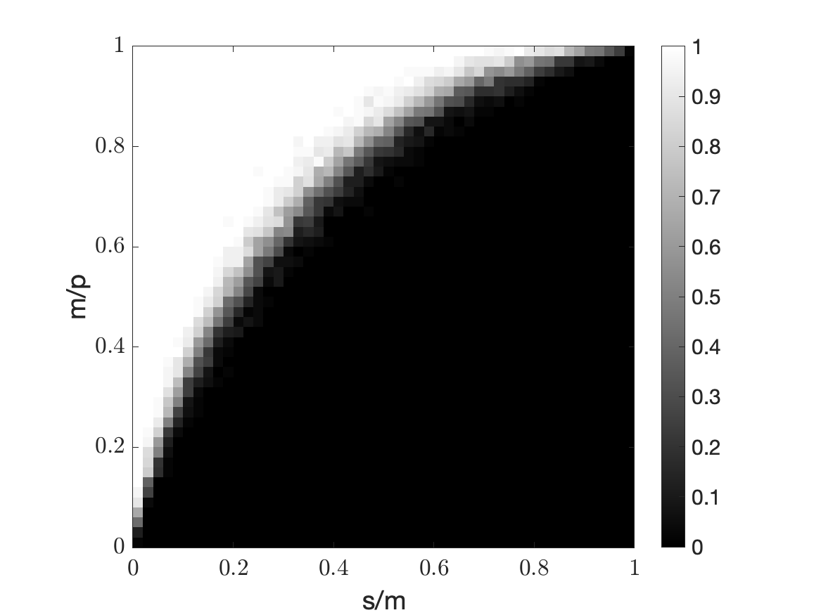
While there are obvious similarities between Johnson-Lindenstrauss projections and sensing matrices that satisfy the RIP, there are also important differences.9898 98 Interestingly, there are known relationships between the two objects [261]. We note that for JL dimension reduction to be applicable (an upper estimate of ) the number of vectors must be known a priori (and this number if finite). JL projection preserves (up to ) pairwise distances between these vectors, but the vectors do not have to be sparse. As a consequence, JL projections are, in general, a one-way street, as in general one cannot recover from . In contrast, a matrix that satisfies the RIP works for infinitely many vectors, however with the caveat that these vectors must be sparse. Moreover, one can recover such sparse vectors from (and can do so numerically efficiently).
As a consequence of these considerations, a matrix that satisfies the RIP does not necessarily have to satisfy the Johnson-Lindenstrauss Lemma. While a Gaussian random matrix does indeed satisfy both, RIP and the Johnson-Lindenstrauss Lemma, other matrices do not satisfy both simultaneously. For example, take a randomly subsampled Fourier matrix of dimensions . In the notation of the definition of the Fast Johnson-Lindenstrauss transform, this matrix would correspond to , but without the diagonal matrix that randomizes phases (or signs) of . This matrix will not meet the Johnson-Lindenstrauss properties of Theorem 7.1. But the absence of the phase randomization matrix is not a hurdle for to satisfy the RIP under appropriate conditions on the matrix dimensions.
Indeed, it is known [93] that if , then the partial Fourier matrix satisfies the RIP with high probability. The exact number of logarithmic factors needed is the object of much research with the best known upper bound due to Haviv and Regev [215], giving an upper bound of . On the side of lower bounds it is know that the asymptotics established for Gaussian matrices of are not achievable in general [39].
Checking whether a matrix satisfies the RIP or not is in general NP-hard [36, 419]. While Theorem 15.9 suggests that RIP matrices are abundant for , it appears to be very difficult to deterministically construct matrices that satisfy RIP for , known as the square bottleneck [411, 38, 37, 40, 78, 318]. The only known unconditional construction that is able to break this bottleneck is due to Bourgain et al. [78]; their construction achieves for a small, but positive, . There is also a conditional construction, based on the Paley Equiangular Tight Frame [38, 40].
In Section 66.1 we will consider more practical conditions for designing sensing matrices. These conditions, which are better suited for applications, are based on the concept of the coherence of a matrix. Interestingly, the phase randomization of that is notably absent in the partial Fourier matrix mentioned above, will reappear in this context in connection with nonuniform recovery guarantees.
Remark 15.2.
If one is interested in understanding the probability of exact recovery of a specific sparse vector, and not a uniform guarantee on all sparse vectors simultaneously, then it is possible to do a more refined version of the arguments above that are able to predict the exact asymptotics of the number of measurements required; see [109] for an approach based on Gaussian widths and [18] for an approach based on Integral Geometry.
65 Duality and exact recovery
In this section we describe yet another approach to show exact recovery of sparse vectors via (429). In this section we take an approach based on duality, the same strategy we took in Chapter 12 to show exact recovery in the Stochastic Block Model. The approach presented here is essentially the same as the one followed in [179] for the real case, and in [422] for the complex case.
In Chapter 8 we derived the dual of a Linear Program using the Lagrangian formulation (we recommend the reader to work out the alternative derivation using the game theoretic approach used in Chapter 12 (there it was used to derived the dual of a Semidefinite Program). The dual to the Linear Program (430) is given by:
| (445) |
Weak duality (the fact that ) is, as usual, easy to verify: If and are primal feasible and is dual feasible, then
| (446) | |||||
showing that . Furthermore, we know from Chapter 36 that strong duality holds, and it guarantees that the optimal values of the two programs actually match.
65.1 Finding a dual certificate
In order to show that is an optimal solution9999 99 For now we will focus on showing that it is an optimal solution, see Remark 15.3 for a brief discussion of how to strengthen the argument to show uniqueness. to (430), we will find a dual feasible point for which the dual matches the value of in the primal, is known as a dual certificate that we introduced in Chapter 36.3.
From (446) it is clear that must satisfy
the complementary slackness condition from Chapter 36.3. This means that we must take the entries of be or when is non-zero (and be when it is positive and when it is negative), in other words
where , and (in order to be dual feasible).
Remark 15.3.
It is not difficult to see that if we further ask , any optimal primal solution would have to have its support contained in the support of . Indeed, extending Theorem 8.16 to the case when the objective is not differentiable but has a subdifferential (as is the case for ), and then using the properties of the subdifferential for the -norm that we computed in Chapter 36.5, gives the following lemma.
Lemma 15.10.
Consider the problem of sparse recovery discussed above. Let , if is injective and there exists such that
and
then is the unique optimal solution to the -minimization problem (429).
Since we know that (and that is injective), we try to construct100100 100 Note how this differs from the situation in Chapter 12 where the linear inequalities were enough to determine a unique candidate for a dual certificate. by least squares and hope that it satisfies . More precisely, we take
where is the Moore-Penrose pseudo-inverse of . This gives the following corollary.
Corollary 15.11.
Consider the problem of sparse recovery. Let . If is injective and
then is the unique optimal solution to the -minimization problem (429).
Theorem 15.9 establishes that if , for a universal constant , and is drawn with i.i.d. Gaussian entries then101101 101 Note that the normalization here is taken slightly differently: entries are normalized by , rather than , but the difference is negligible for our purposes. it will, with high probability, satisfy the -RIP. Note that, if satisfies the -RIP then, for any one has and , where denotes the operator norm .
This means that if we take random with i.i.d. entries then, for any we have that
and because of the independency among the entries of , is independent of this vector and so for each we have
where is the -th column of .
An application of the union bound gives
which implies
which means that we expect to exactly recover via minimization when . While this can be asymptotically worse then the bound of , and this guarantee is not uniformly obtained for all sparse vectors, the technique in this section is generalizable to several circumstances and illustrates the flexibility of approaches based in construction of dual witnesses. We will discuss nonuniform guarantees in more detail in the next section.
66 From theory to practice
66.1 Sensing matrices and incoherence
In applications, we usually cannot completely freely choose the sensing matrix to our liking. This means that Gaussian random matrices play an important role as benchmark, but from a practical viewpoint they play a marginal role. Clearly, randomness in the sensing matrix seems to be very beneficial for compressive sensing. However, in practice, there are numerous design constraints on the sensing matrix , as in many applications one only has access to structured measurement systems. For example, we may still have the freedom to choose, say the positions of the antennas in radar systems that employ multiple antennas [403, 406], the position of sensors in MRI [298, 7, 72, 339], or the sampling locations in digital signal acquisition [317]. By choosing these randomly, we can still introduce randomness in our system. Or, we can transmit random waveforms in sonar and radar systems [217, 359]. Yet, in all these cases the overall structure of is still dictated by the physics of wave propagation. In other applications, it will be other physical constraints or design limitations that will dictate how much randomness we can introduce into the sensing matrix.
While establishing the RIP (with high probability) for Gaussian or Bernoulli random matrices is not too difficult, it is already significantly harder to do so for the partial Fourier matrix [93, 378, 215] and time-frequency matrices [156], and even harder for more specific sensing matrices.
A useful concept to overcome the practical limitations of the RIP is via the concept of the (in)coherence of a matrix. This concept has proven to be widely applicable in practice. While we want to avoid the constraints of the RIP, we nevertheless take it as our point of departure. Recall that the RIP (Definition 15.6) asks that any , satisfies:
for all . This is equivalent to
or equivalently
If the columns of are unit-norm vectors (in ), then the diagonal of is all-ones, this means that consists only of the non-diagonal elements of . If, moreover, for any two columns , , of we have for some then, Gershgorin’s circle theorem tells us that .
More precisely, given a symmetric matrix , the Gershgorin’s Circle Theorem [226] states that all of the eigenvalues of are contained in the so called Gershgorin discs (for each , the Gershgorin disc corresponds to
If has zero diagonal, then this reads: .
Given a set of unit-norm vectors we define its worst-case coherence as
| (447) |
Assume now the vectors have worst-case coherence . If we form a matrix with these vectors as columns, then it will satisfy the -RIP, implying that it will satisfy the - RIP for .
This motivates the problem of designing sets of vectors with smallest possible worst-case coherence. This is a central problem in Frame Theory [404, 121, 107, 452]. Recall that in finite dimensions, a set of vectors (where or ) is called a frame for if there exist constants (frame bounds) such that102102 102 Since here we are dealing with a finite dimensional Hilbert space, the upper frame bound is always trivially fulfilled, and the lower bound is equivalent to the the frame forming a spanning set.
| (448) |
for every . The associated frame operator is defined by
| (449) |
The frame definition (448) can be equivalently expressed as requiring that holds, where denotes the positive-semidefinite order. A frame is called tight if , in which case . If for all then is called a unit norm frame. We call a unit norm frame equiangular if
| (450) |
for some constant . Obviously, any orthonormal basis is equiangular.
We can now provide an elucidating answer to the question of a lower bound on the coherence of a set of vectors via the following theorem from frame theory.
Theorem 15.12 ([404]).
Let be a unit-norm frame for , where or Then
| (451) |
Equality holds in (451) if and only if is an equiangular tight frame.
Proof.
A simple calculation shows that
Let be the eigenvalues of . Let 1 denote the all-one vector. By the Cauchy-Schwarz inequality
which can be stated equivalently as
| (452) |
Equality holds in (452) if and only if , i.e., if and only if is a tight frame
We now consider
| (453) |
with equality if and only if is equiangular. By the bound (452) we have
| (454) |
with equality if and only if is a tight frame. Inequalities (453) and (454) together give (451) and the proof is complete.
∎
We note that if equality in (451) can only hold if , while if then equality in (451) can only hold if . This can be shown by a so-called tensoring trick (we invite the reader to try): by analyzing the gram matrix of the vectors (the and bounds then appear by the dimension of the subspace in which these vectors lie), see Table II of [138].
The coherence bound (451) of a set of unit-norm vectors in dimensions is also known as Welch bound [457]. Due to this limitation implied by Theorem 15.12, deterministic constructions based on coherence cannot yield matrices that satisfy the RIP for , known as the square-root bottleneck [38, 411, 78, 40].
However, as we will see in Section 66.2, if we are willing to accept slightly weaker recovery guarantees than provided by the RIP, matrices with low coherence do give rise to sensing matrices that come with appealing theoretical guarantees while also being useful in practice.
Theorem 15.12 suggests that in order to design sensing vectors of minimal coherence, we should look for equiangular tight frames (ETFs). The existence and construction of ETFs is a rather challenging problem that intersects with a wide range of areas such as harmonic analsyis, algebraic, combinatorics, finite geometry, group theory and representation theory, and coding theory [404, 452]. Applications include signal processing, wireless communications, numerical linear algebra, and quantum physics. Indeed, ETFs are deeply connected to Zauner’s conjecture, particularly through their role in quantum information theory and the concept of SIC-POVMs (Symmetric Informationally Complete Positive Operator-Valued Measures) [469, 384, 23].
Another interesting and very useful construction of sensing vectors with low coherence is given by so-called mutually unbiased bases [464, 162, 50, 89, 404]. These bases are widely used in quantum information theory as well as in radar and signal processing. Two orthonormal bases are called mutually unbiased if and only if
| (455) |
The classical example of an MUB consists of the identity matrix and the Discrete Fourier transform matrix concatenated into a matrix. But, perhaps surprisingly, for certain values of , there exist MUBs in consisting of orthonormal bases such that condition (455) is satisfied for any two orthonormal bases , see for example [464, 50, 89, 404, 12]. Thus, MUBs give rise to structured sensing matrices of dimension with coherence , which thus almost achieve the Welch bound. Here is a simple example for an MUB in : Let be a prime number and set for . Then the vectors defined via
| (456) |
satisfy for all , which follows from basic properties of quadratic Gauss sums (cf. Theorem 2 in [12]). We can add the identity matrix and end up with vectors (split into ONBs) in which form a MUB of maximal size. For other, nonequivalent constructions, of MUBs (which, however, still revolve around translations and modulations in form of the finite Heisenberg group) see [89]. Remarkably, for not a power of a prime number it is not known how many MUB exist; this is an open problem even for [48]. For the construction and existence of MUBs faces more constraints. Even the existence of two bases is equivalent to the existence of so-called Hadamard matrices ( matrices with orthogonal columns) for which the existence for dimensions that are a multiple of is still a (celebrated) open question (see, e.g. [48]).
66.2 Nonuniform recovery guarantees and coherence
As mentioned before, it follows from Theorem 15.12 that deterministic constructions based on coherence cannot yield matrices that satisfy the RIP for , known as the square-root bottleneck [38, 411]. To overcome this square root bottleneck it seems that something has to give. One fruitful direction is to sacrifice the uniform recovery granted by the RIP. Namely, once a matrix satisfies the RIP, it is guaranteed that the solution to the -optimization problem is identical to the solution to the -optimization problem (the sparsest solution) for all -sparse vectors. In contrast, we can consider scenarios in which -optimization and optimization having the same solution holds “only” for most -sparse vectors. This leads to nonuniform recovery results, which we will pursue below. The benefits however are often worth the sacrifice, since we end up with theoretical guarantees that are much more practical.
Recall that we consider a general linear system of equations , where , and . We introduce the following generic -sparse model:
- (i)
The support of the nonzero coefficients of is selected uniformly at random.
- (ii)
The non-zero entries of form a Steinhaus sequence, i.e., is a complex random variable that is uniformly distributed on the unit circle, and independent from each other (and from ).
As an example for a theoretical nonuniform guarantee using coherence-based sensing matrices we state (without proof) the following theorem, and refer to [174] for a proof.
Theorem 15.13 (Theorem 14.5 in [174]).
Let , be a matrix with -normalized columns and coherence . Let be a subset of selected at random according to the uniform model with . Let be a vector supported on for which is a Steinhaus sequence independent of . Assume that, for
| (457) | ||||
| (458) |
for an appropriate constant . Then, with probability at least, the vector is the unique minimizer of subject to .
A simple calculation shows that for a unit-norm tight frame the condition 457 is satisfied if
which is in the ballpark of condition (444) for Gaussian sensing matrices. Theorem 15.13 demonstrates that by allowing for nonuniform recovery guarantees one can successfully reconstruct sparse signals under much milder coherence conditions than imposed by the aforementioned square root bottleneck. That being said, establishing that the support set of real-world signals can be modeled as random is, in general, difficult to justify rigorously. For instance, the wavelet coefficients of natural images are typically concentrated along edges, giving rise to structured, tree-like patterns in the locations of significant coefficients. This insight is utilized in practical compressive sensing systems as, for example, in MRI [298, 7]. The fact that the support set of many natural signals does not conform to a uniform distribution highlights the relevance of the recovery results established in Sections 62–64, which hold for all sufficiently sparse signals. Furthermore, as pointed out in [174], the stability guarantees currently available for models based on random supports are notably weaker than those derived from the restricted isometry property.
66.3 Further practical considerations
When moving the ideas of compressive sensing to move from theory into practice we encounter some challenges: (i) the choice of the sensing matrix is often limited by practical considerations and physical constraints (both usually rule out a Gaussian sensing matrix); (ii) signals are often not sparse in the measurement domain, but only with respect to some properly chosen transform (and even then, signals are often only approximately sparse); (iii) for various reasons (speed being one of them) we may need alternative sparse solvers instead of vanilla -minimization. We already have discussed (i) earlier in this section and will discuss items (ii) and (iii) succinctly below. We recommend [7] for a detailed treatment of how to span the gap between theory and practice of compressive sensing.
As indicated above, signals are often not sparse in the canonical basis, but they are (approximately) sparse after a suitable transformation. For examples audio signals are sparse with respect to a localized Fourier transform such as a Gabor transform [135] or some other local trigonometric transform [303, 302]. JPEG exploits the sparsity of images in the discrete cosine basis or wavelet basis [302] while curvelet transforms are effective sparsifiers for images arising in astronomy [396]. Radar signal are sparse when (properly) transformed into the time-frequency domain [217]. Some signals may even require a redundant dictionary (perhaps consisting of a combination of a wavelet basis, a curvelet basis, and a Fourier basis), see e.g. [302, Chapter 12]. But how do such transform-sparse signals fit into our framework?
As before, let be the signal (or image) of interest and we observe , where is a sensing matrix, where . We assume that is sparse with respect to some basis or frame , where (and if we restrict to be a basis). Denote this sparse representation by , i.e., . We write and can now solve for via
| (459) |
Having solved this problem (assuming it does indeed yield ), we can recover from by simply computing .
Thus, we can (try to) apply the theoretical results developed in the previous sections to the matrix in place of . In a nutshell, the sensing matrix has to be incoherent with respect to the transform in which the signal is sparse. An important example arises in MRI. There, the wavelet transform is often chosen as sparsifying transform and the sensing matrix is derived from randomly subsampling the two-dimensional Discrete Fourier Transform or the Radon transform, see [298, 7]. In practice, it has been observed that even better results are obtained when the random subsampling of the Fourier coefficients is combined with a deterministic sampling of the Fourier coefficients corresponding the low frequencies, a strategy that has already been suggested in one of the original papers on compressive sensing [155]. We refer to [298, 7] for many more details and modifications.
Figure 73 shows an example of compressive sensing applied to MRI. The test image is the so-called GLPU phantom (introduced by Guerquin-Kern, Lejeune, Pruessmann and Unser in [203]). It is a continuous, piecewise constant MRI-type image with an analytic expression for its Fourier transform. The reconstruction of the discrete GLPU phantom from 30% randomly chosen discrete Fourier measurements. The wavelet transform with a Haar wavelet has been used as sparsifying transform . The image is recovered by first solving (459) for , followed by computing .

There are various other efficient and rigorous methods to recover sparse vectors from underdetermined systems besides -minimization and the lasso. For example, homotopy methods, greedy algorithms or methods based on approximate message passing. We refer to [174, 7] for a comprehensive discussion of these techniques. Furthermore, [7] contains a detailed discussion of some subtle potential numerical stability issues one should be aware of.
Exercises
Exercise 15.1 (Sparse vector approximation in ).
Let be integers and be a vector. Show that there exists an -sparse vector such that
Exercise 15.2 (-Minimization Recovery).
Let be a matrix. Suppose that every -sparse vector can be uniquely recovered by via minimization, i.e, we choose that minimizes subject to the constraint and is the unique minimum of this problem if has at most nonzero entries.
- 1.
Prove that every columns of are linearly independent.
- 2.
Prove that .
- 3.
Prove that if a matrix satisfies the condition that every columns are linearly independent, then every -sparse vector can be uniquely recovered by via minimization.
Exercise 15.3 (Stable nullspace property).
A fundamental fact in compressed sensing is that in order to recover an -sparse vector by minimizing the norm, the measurement matrix needs to satisfy the null space property. The goal of this exercise is to study the compressed sensing problem when is approximately sparse.
We say that a matrix satisfies the -stable null space property if for every non-zero vector and all sets such that , the following holds
Prove the following facts
- 1.
Given a set and vectors ,
- 2.
Prove that if satisfies the -stable nullspace property with , then the solution of the optimization program
satisfies
where is the -best term approximation error of , given by .
- 3.
Show that the stable nullspace property with is sufficient for exact recovery when the vector is -sparse.
Exercise 15.4.
Let and set
Using the null space property, show that -minimization will recover any 1-sparse vector , given .
Exercise 15.5.
On the connection between (in)coherence parameter and restricted isometry constant : Show that , and .
Exercise 15.6.
Let be a Gaussian random matrix. Give an estimate for the coherence of .
Exercise 15.7.
The proximal operator for the norm is defined as
Derive the closed-form solution (Soft-Thresholding) for .
Exercise 15.8.
Consider , where is a Gaussian random matrix and is an -sparse vector of length 400. The locations of the non-zero entries of are chosen uniformly at random and the non-zero coefficients of are normal-distributed. For solve
(e.g. using the Matlab toolbox cvx, see cvxr.com/cvx, or its Python version cvxopt or its R version cvxr.). For each fixed repeat the experiment 10 times. Create a graph plotting versus the relative reconstruction error (averaged over the ten experiments for each ). Starting with which value of (approximately) does -minimization fail to recover ?
Exercise 15.9.
Same setup as in the previous exercise, but now the non-zero entries of are non-negative. Taking this information into account, we now solve
(here, is meant entrywise, i.e., for each ). (The positivity constraint is easy to include in cvx). Repeat the simulations as described in the previous exercise. Compare your findings to the results from your experiments of the previous exercise and try to quantify the difference regarding the range for for which recovery is still possible in this case.
Exercise 15.10.
Let be a prime number and set
for . Define the vectors
Prove that these vectors plus the unit vectors together form a mutually unbiased basis (MUB) of vectors for .
Exercise 15.11.
This exercise is a bit more involved. It asks you to prove Zauner’s Conjecture, a
fascinating conjecture that pervades many areas of mathematics, including quantum information theory, harmonic analysis and frame theory, finite group theory and representation theory, algebraic number theory, algebraic geometry, discrete and combinatorial geometry, operator algebras, and matrix analysis.
(If you actually succeed in proving Zauner’s Conjecture, T.S. will send you one of the famous Zaunerstollen (different Zauner) as reward; and you may also become a serious contender for significant mathematical awards).
Zauner’s Conjecture: [469, 367] For every integer , there exists a unit vector (called a fiducial vector such that its orbit under the Weyl–Heisenberg group,
forms an equiangular tight frame of vectors in . Here is the cyclic translation operator defined by where and (thus the translation index is computed modulo ) and is the modulation operator defined by for .
Chapter 16 Low-Rank Matrix Recovery
Low-rank matrices arise throughout the sciences because many high-dimensional datasets are governed by a small number of latent factors, leading to strong correlations among variables [433]. Low-rank matrix recovery is a fundamental problem in mathematics and computer science that deals with recovering a matrix from incomplete measurements [465]. What does incomplete mean in this context? Consider for example a matrix . Then, is determined by parameters. Assume we are given measurements of this matrix with . Without any further assumptions, the problem of recovering from these measurements is ill-posed in this case, admitting infinitely many solutions. But what if is a low-rank matrix? Can we recover a low-rank matrix from fewer measurements, and if so, can we do it in a numerically robust and efficient manner? And what other conditions do the measurements have to satisfy to make such an endeavour possible? These are the questions we intend to answer in this chapter.
A prominent example of matrix completion and low-rank modeling is collaborative filtering, widely used in recommender systems [260, 8, 432]. Imagine a user-item rating matrix , where represents the rating given by user to item . Most entries in this matrix are typically missing, as users usually rate only a small fraction of the available items. The goal of collaborative filtering is to predict the missing ratings, allowing the system to recommend relevant items to users. By assuming that the rating matrix is approximately low-rank (reflecting latent factors like user preferences and item characteristics), we can use matrix completion techniques to infer the missing ratings and provide personalized recommendations. A famous example is the “Netflix Prize” competition conducted between 2006 and 2009, see [67] for details.
An important application of low-rank matrix recovery arises in quantum tomography [200]. In this context, the matrix represents the density matrix of a quantum system. Due to limitations in measurement devices, we often can only obtain incomplete information about the density matrix. The density matrix is a positive semi-definite matrix with trace 1, and often, it is low-rank, especially for systems in a mixed state or when only a limited number of degrees of freedom are accessible. Matrix completion techniques can be used to reconstruct the full density matrix from the incomplete measurements. This reconstruction is crucial for characterizing the state of the quantum system and performing quantum information processing tasks. The low-rank assumption is justified by the physical nature of many quantum states, and carefully exploiting it allows for efficient and robust state reconstruction.
Other applications of matrix recovery and low-rank modeling arise in link prediction in social networks [118, 310], Euclidean distance matrix embedding [237, 149], robust photometric stereo [465], phase retrieval [94], blind deconvolution [9], and self-calibration [287]. We will discuss some of these applications in more detail later in this chapter.
As the reader may suspect, there are strong connections between compressive sensing and low-rank matrix recovery. The connection lies in the fact that both rely on parsimonious structural assumptions (sparsity for compressive sensing and low-rank for matrix recovery) and can be tackled using convex relaxation. In both cases, the idea is to exploit these structures to recover the original data efficiently despite having far fewer observations than the ambient dimension of the signal of interest. Thus, it is not surprising that throughout this chapter we will see many parallels to compressive sensing. Nevertheless, matrix recovery poses some additional challenges, as the attentive reader will discover.
67 Rank minimization and the nuclear norm
We will refer to a matrix as low-rank if its rank is small compared to . The choice that is real-valued is just for convenience, but all results can easily be adapted to the complex-valued setting. A simple computation reveals that such an has degrees of freedom, which corresponds to the dimension of the tangent space to the manifold of rank- matrices.
We write for the Hilbert space of all Hermitian matrices equipped with the Hilbert-Schmidt inner product We will also deal with linear transformation which acts on the space , we will use calligraphic letters to denote these operators, as in .
Now, consider a matrix with rank . and assume we are given measurements of the form
| (460) |
where the are some matrices in . For notational convenience, we define the measurement operator
| (461) |
Thus, we can express the (possibly noisy) matrix measurement process in compact form via
where contains all measurement outcomes and denotes additive noise.
For reference, the adjoint operator maps real-valued inputs into Hermitian matrices, and is given by
Let us first consider the noiseless case. A natural approach to recovering is to solve the rank minimization problem
| (462) | ||||
This formulation directly encodes the assumption that the solution should have minimal rank among all matrices consistent with the measurements.
In a few cases, rank-minimization problems can be solved explicitly and efficiently. Consider for example the problem
| (463) | ||||
where is a given matrix. Let denote the SVD of . Utilizing our findings in Chapter 10.3, it is easy to see that the solution is given by a properly truncated SVD of , namely , where is the smallest number such that .
However, the rank function is non-convex, discontinuous, and combinatorial in nature. As a result, rank minimization problems are NP-hard in general, even in seemingly simple settings [439, 168]. One way to see this is by considering the special case where is a diagonal matrix. In that case we have and the rank minimization problem takes the form
| subject to |
which played a central role in Chapter 15, and we already know it to be NP-hard [330, 174].
This computational intractability motivates the search for tractable relaxations that retain the essential structure of the original problem.
A standard convex surrogate for the rank function is the nuclear norm, defined as
where are the singular values of . The nuclear norm is convex and can be viewed as the matrix analogue of the -norm for vectors, which is known to promote sparsity. In fact, the nuclear norm is the tightest convex lower bound of the rank function on the unit spectral-norm ball, see e.g. Theorem 1 in [167]. Compare also Figure 74 to Figure 71(a).

Replacing the rank objective in (462) by the nuclear norm yields the convex optimization problem [168, 97, 365]
| (464) | ||||
This problem can be cast as a semidefinite program (see Exercise 16.6). Consequently it can be solved efficiently using interior-point methods for moderate problem sizes or first-order methods for large-scale instances.103103 103 Generally, first-order methods have better time-complexity dependency on the problem size, but worse dependency on the desired distance to optimality.
In the presence of noise, i.e,, , where represents the noise term, one typically considers a relaxed formulation
| (465) | ||||
where is an upper bound on the error, that is .
Although nuclear norm minimization is only a relaxation of rank minimization, it has been shown to recover the true low-rank solution exactly under suitable conditions on the measurement operator . These conditions can be expressed in various ways, including restricted isometry properties, incoherence assumptions, or geometric criteria based on descent cones and Gaussian width.
The success of the convex relaxation is therefore not accidental: the nuclear norm captures the essential geometry of low-rank matrices in a way that allows both computational tractability and provable recovery guarantees, similarly to how the does for Sparsity (Chapter 15). As a result, nuclear norm minimization has become a cornerstone of modern low-rank matrix recovery theory. We will explore this topic in more detail in the next sections.
68 Recovery guarantees via descent cone analysis
A central challenge in low-rank matrix recovery is to determine when a convex optimization procedure---typically nuclear norm minimization---can exactly recover a matrix of low rank from a set of linear measurements. A powerful and general framework to analyze this question arises from descent cone104104 104 The descent cone is sometimes equated to the tangent cone from convex geometry, although technically they do not usually coincide. analysis and conic geometry, developed in [109, 18, 430] and refined in numerous followup papers, such as [266, 1, 180]. Our analysis will follow in part the perspicuous presentations in [430, 180].
Definition 16.1.
The descent cone of a proper convex function105105 105 A proper convex function is an extended real-valued convex function with a non-empty domain, that never takes on the value and also is not identically equal to . at a point is the conic hull of directions in which decreases near
The descent cone of a convex function is always a convex cone, but it may not be closed.
The descent cone analysis approach is widely applicable. In connection with low-rank matrix recovery, we are concerned with the case where .
Consider now the following two convex optimization problems:
| (466) | ||||
| (467) | ||||


We start with the noiseless case. If is the ground truth to , then any minimizer of (466) must satisfy and . This implies that can be decomposed into , where . If the intersection between the nullspace and the descent cone only contains the zero element, then must be the unique optimal solution to (466), as illustrated in Figure 75(a).
In the noisy case, we cannot ask for exact recovery. But in light of (467) we hope that the error between a solution and the ground truth is of the order of . Let be a feasible solution of (467) and note that the constraint implies . Thus, to bound the error , we need to focus our attention on the intersection of and . The smaller the size of the intersection, the smaller the error will be, cf. also Figure 75(b).
The size of can be controlled by a quantity called the smallest conic singular value106106 106 The terminology originates in the fact that coincides with the usual minimum singular value of . [430, 109, 180], which is defined by
| (468) |
The following proposition shows that when is large, the size of the intersection will be small, which in turn would yield a smaller error [430, 109, 180].
Proposition 16.2.
Let be a linear operator and assume that with . Then, any minimizer of the optimization problem (467) satisfies
| (469) |
Proof.
We have
| (470) |
for any feasible . Here, the first inequality in (470) follows from the definition of , the second inequality from the triangle inequality, and the third one from and the assumption . Rearranging the terms in (470) concludes the proof.
∎
As a consequence, if we can show that , then this would imply exact recovery in the noiseless scenario. However, Proposition 16.2 is deceptive in its simplicity. In general it is actually rather difficult to compute or bound the smallest conic singular value of a matrix. The situation becomes more promising once we introduce randomness in the measurement process, and thereby into . We will explore such a scenario next.
68.1 Low-rank matrix recovery from Gaussian measurements
We consider the case of low-rank matrix recovery with measurements of the form
where the are Gaussian matrices.
The proof strategy to bound for this Gaussian measurement operator is based on Gordon’s Theorem, the use of which was first proposed in the context of sparse recovery by Rudelson and Vershynin in [378, Section 4]. It revolves around the concept of Gaussian width, which we introduced in Definition 13.14.
Setting , our goal becomes to bound from below. Revisiting Gordon’s Theorem, an inspection of the proof of Theorem 13.16 (in particular (408)) yields the following tail bound107107 107 The observant reader might have noticed that in (471) we have replaced the minimum in (406) by the infimum. This switch (the verification of which is left to the reader) is due to the fact that the descent cone may not be closed.
| (471) |
with probability at least , where we have used the well known bound in (406) and to adapt the notation in Chapter 13 to the current setting ( denotes the number of measurements in this chapter). If does not exceed , then we can obtain probabilistic recovery guarantees via Proposition 16.2.
As pointed out in [180], Gordon’s Theorem—and therefore also the tail bound in (471)—only requires to be a subset of the Frobenius unit sphere108108 108 The Frobenius unit sphere is . . Therefore, one is not restricted to a specific descent cone but one can instead choose the union over all possible descent cones corresponding to rank- matrices in order to obtain uniform recovery guarantees:
Proposition 16.3 ([180], Corollary 2.1).
The Gaussian width of , the union over all possible descent cones with an anchor point of rank- can be bounded by
Furthermore, let be a Gaussian measurement operator. Then, is bounded away from zero for any rank- matrix X w.h.p. if
The proof of Proposition 16.3 makes use of the following result, which we state without proof.
Lemma 16.4 ([180], Lemma 2.2).
Suppose that is contained in the nuclear norm descent cone of a rank- matrix . Then,
of Proposition 16.3.
Using Hölder’s inequality and Lemma 16.4, the Gaussian width can be bounded in terms of the expected operator norm of a standard Gaussian matrix:
where in last inequality we have used the bound , which can be found in e.g. [445, Remark 4.4.4]. Using the tail bound (471) derived from Gordon’s Theorem, we obtain
with probability at least . Therefore, if
we can pick , such that is positive w.h.p. ∎
69 Low-rank matrix recovery and dual certificates
The descent cone approach, while geometrically appealing, faces arduous challenges109109 109 Some, but not all, of these challenges can be addressed by employing Mendelson’s small ball method, see [309, 258, 430, 180]. when we deal with problems where additional structure, such as incoherence of the unknown signals, is critical to exclude exceptional instances where the reconstruction must necessarily fail (see [180] for a more detailed discussion of the issues that arise). Thus, in applications like quantum state tomography, phase retrieval, and matrix completion, an approach based on dual certification introduced in Chapter 36, is often preferable.
The next lemma will pave the way to establishing tractable conditions that the nuclear norm relaxation (464) attains its optimal value at a specific point is through the provision of a dual certificate (sometimes also called dual witness).
Recall from our computation of the subdifferential of the nuclear norm in Chapter 36.5 the definition the tangent space at a rank matrix with SVD relative to the manifold of rank- matrices:
Lemma 16.5 (Dual certificate, [96]).
Let be such that . Assume that the following two conditions hold:
- 1.
There exists a vector such that satisfies
(472) - 2.
The linear operator is injective when restricted to the tangent space .
Then is the unique minimizer of (464).
Proof.
Suppose is feasible and has SVD with . Let and denote the orthogonal projections on and , respectively.
The Lagrangian is
The KKT conditions for optimality of are (note that we do not have inequality constraints): (i) Primal feasibility: . (ii) Dual feasibility: . (iii) Complementary slackness: these are trivially fulfilled here since all constraints are equalities. Thus, to certify optimality it suffices to construct a such that
We have seen in (273) that
So any matrix of the form
is a valid subgradient.
Suppose now there exists such that and . We will show that this implies .
Write
where . By assumption, and , thus all conditions in (273) are satisfied, and therefore . Since is feasible and , the KKT conditions hold, so is optimal.
If additionally
then one can show that for any feasible ,
hence is the unique minimizer. This follows from the subgradient inequality
with equality only if .
∎
The hard part is now to verify that a given measurement operator actually satisfies the conditions of Lemma 16.5, in particular condition (472). One of the most successful and widely applicable approaches for this relies on the so-called golfing scheme, introduced by David Gross [201]. In [201] Gross demonstrates that the conditions in Lemma 16.5 can be relaxed and that the existence of an approximate dual certificate suffices to establish uniqueness and this approximate dual certificate can be constructed via the golfing scheme in an iterative manner110110 110 In [180] it is shown that a minor modification of the golfing scheme gives an explicit randomized construction for an exact dual certificate, which does not use more measurements than the original argument..
The concept of an approximate dual certificate allows for small errors on the tangent space and a margin of safety on the orthogonal complement .
Definition 16.6.
A matrix is an -approximate dual certificate for if it satisfies the two conditions:
- 1.
Alignment on : , (473) - 2.
Constraint on : . (474)
The operator will play an important role in our subsequent analysis. It dictates how much of a signal can hide in the kernel of the operator relative to its projection onto the tangent space . The next lemma quantifies the “spectral-to-Frobenius” leakage. It ensures that any matrix in the kernel of the measurement operator cannot have its energy concentrated in the “signal” space without having significantly more energy in the “noise” space .
Lemma 16.7 (Leakage Lemma).
Let be a measurement operator. For any , the following inequality holds
where the leakage constant is defined as
and denotes the smallest eigenvalue of .
Proof.
Since , we have and . Lower Bound (RIP on ): Let . For any , we have . Applying this to gives
We have
Applying Cauchy-Schwarz and induced norms gives
Dividing both sides by establishes the desired bound. ∎
Theorem 16.8.
Let be a rank- matrix with tangent space . Suppose there exists an -approximate dual certificate . with leakage constant such that , then is the unique minimizer of the nuclear norm minimization problem (464).
Proof.
We must show that for any non-zero , .
By the definition of the nuclear norm subgradient at
Since and , we have . Thus
Substituting this identity into the subgradient inequality gives
By Hölder’s inequality,
Using Cauchy-Schwarz gives . We now apply the Leakage Lemma and obtain . Hence,
Since for any matrix we get
If , the term in the parentheses is strictly positive, which implies that . ∎
Remark 16.1.
The approach we have just outlined using the approximate dual certificate and the Leakage Lemma is essentially a dual-space perspective on the primal-space descent cone geometry that we described in Chapter 68. In the descent cone approach we ask how much the operator “shinks” vectors that are trying to decrease the nuclear norm. If the smallest conic singular value is large, the operator captures these directions, and they cannot be in the kernel. In the approximate dual certificate approach the leakage constant quantifies how much a kernel element can “hide” its energy in the tangent space. A large smallest conic singular value corresponds to a small leakage constant (but not in a way that allows us to easily convert one into the other).
The reader may wonder whether so far we just have been ‘kicking the can down the road’, since we moved from the primal problem to the dual certificate to the approximate dual certificate to the leakage constant. After all, while Theorem 16.8 proves that a certificate allows for recovery, it still does not tell us how to find one.
Fortunately111111 111 This is not a fortunate coincidence, but rather fortune that favors the prepared mathematician., there are now several techniques at our disposal to address this critical issue. One such technique is the aforementioned golfing scheme. It provides an ingenious algorithm to build by successively projecting the “residual error” from the tangent space back into the range of the measurement operator. The concrete application of Theorem 16.8 and the golfing scheme will depend on the specific nature and setting of the low-rank problem under consideration. In the following we will explore three compelling applications, matrix completion, quantum state tomography, and phase retrieval.
While the overall proof architecture via approximate dual certificate and golfing scheme is shared across all three applications, the specific mathematical properties of the measurements affects key steps in the proofs significantly. The difficulty in each proof lies in how the specific measurement operator interacts with the Tangent Space .
70 Matrix completion
Matrix completion is the problem of recovering an unknown matrix from a subset of its entries, under the assumption that the matrix has low rank [97, 104]. Cast in the form of (460), this means that the measurement matrices take the form , whence , i.e., the measurements reveal individual entries of the matrix. We define the sampling operator , where , where is some subset of the complete set of matrix entry indices . Thus, in the notation of (460), and .
Without further knowledge the problem of recovering from the entries is ill-posed and has infinitely many solutions—just fill in the missing entries with arbitrary values. But assuming that is a low-rank matrix, can we then fill in the missing entries of in a unique way and can we do so in a numerically feasible way? This problem arises for example in recommender systems, collaborative filtering (user–item ratings, preferences), crowdsourcing and survey data [260, 465, 8, 432].
By counting degrees of freedom of , it is apparent that for low-rank matrix completion we need at least many measurements. But this condition will in general not suffice. Take for example a rank-one matrix whose entries are all zeros, except for, say, its very first entry which we set equal to one. Since a priori we do not know the location of the non-zero entry, in the worst case we would need to take measurements (equal to the ambient dimension of the matrix) in order to successfully complete all missing matrix entries.
This should not come as a complete surprise, since we have encountered a similar situation in compressive sensing. There, we had to impose some notion of incoherence (e.g., via the RIP or directly via the concept of coherence) in order to develop a non-trivial, compelling theory (and numerics) of sparse recovery. We will need to do something similar for matrix completion. In Chapter 66.1 (see equation (447)) we introduced the concept of the (in)coherence of a set of vectors. For matrices we follow the notion of (in)coherence introduced in [97].
Definition 16.9.
Let be a rank- matrix with singular value decomposition , where , . We say that satisfies the incoherence condition with parameter if
Incoherence requires the energy of singular vectors to be spread across coordinates. This prevents “spiky” singular vectors, which would make recovery from few entries impossible. The smallest coherence is 1, achieved if and are spanned by vectors whose entries all have magnitude and , respectively. The largest possible value for is , which would correspond to any or that contains a standard basis element.
We will now apply Theorem 16.8 and the golfing scheme to solve the matrix completion problem, see also [97, 201]
Theorem 16.10.
Assume is a rank- matrix and let be -incoherent. Suppose we observe entries of with locations sampled uniformly with replacement. Then there exists a constant such that if
where , then is the unique minimizer of the nuclear norm minimization problem
with probability at least .
In the proof of Theorem 16.10 we will make use of the following notation. We denote the normalized sampling operator by , where , and the associated subspace projections by and . Note that acts as identity on .
We will employ the following two lemmata. The first one establishes injectivity of the sampling operator on m the second one provides a bound on the leakage constant.
Lemma 16.11.
Proof.
We define the centered random operator . This can be written as a sum of independent, zero-mean operators
We have
where we have used the incoherence assumption in the last step. For the variance we have .
The matrix Bernstein inequality of Theorem 12.5 reads in our setting
| (475) |
Substituting the computed bounds for (the in (475)) and into the exponent of the right-hand side of (475) gives for the exponent
To ensure the probability is less than a small failure tolerance (in this lemma we use ), we set
We take the logarithm, rearrange for , and get
If we treat as a fixed constant (such as e.g., ), the term becomes a constant . Since , we get (by absorbing both constants into )
| (476) |
∎
We point out that the particular choice of only affects the constant in (476).
Lemma 16.12.
Given the assumptions of Theorem 16.10, suppose the number of measurements satisfies . Then with probability at least for every
with leakage constant .
Proof.
Let . As meanwhile usual, we decompose into where . A simple calculation gives
| (477) |
Define the event . We aim to apply the matrix Bernstein inequality to the sum of operators . We compute . And . Hence, by matrix Bernstein, if , then . On , the minimum eigenvalue . Thus
We define the event . Consider the operator . This is a sum of independent operators , restricted to . Note that the induced norm of a rank-1 map is . Hence
For the variance of we compute
Since we get . Applying matrix Bernstein gives for , the probability .
∎
With these two lemmata in place, we are now ready to prove Theorem 16.8.
Proof of Theorem 16.10.
In the proof denotes a constant that may change throughout the derivations. By Theorem 16.8, is the unique minimizer if , and by Lemma 16.12 we have .
We will now construct an -approximate dual certificate iteratively via the golfing scheme. To that end we divide the sampling set into independent batches of about equal size . On the one hand, the size of the batches will have to be chosen large enough to allow for the application of the matrix-valued concentration of measure bounds tailored for independent random variables. On the other hand, the batch size cannot be too large, since the speed of convergence is exponential in . We will determine the proper value of later.
Let be the normalized sampling operator for batch . While taking as the dual certificate does not work since the dual certificate must live in the range of the sampling operator, it still serves as good first initial guess. The idea of the golfing scheme is to iteratively refine this initial guess until condition (473) is fulfilled. We proceed as follows:
- 1.
Initialization:
- 2.
Iteration: and , for
- 3.
Final approximate certificate:
By expanding the recursion, it is easy to see that satisfies
We want to show that is sufficiently close to , which is equivalent to showing that is sufficiently small. From Lemma 16.11, we know that for each batch
with high probability. Therefore,
Iterating this times gives
To make , we set and .
We must also ensure that the “leakage” of the approximate certificate into the orthogonal space remains small, i.e., we want . Expanding gives
Each term is a random matrix. By induced norms,
We can expand into a sum of independent random rank-1 operators and apply the (rectangular) matrix Bernstein inequality. A standard calculation, that is left to the reader, yields
where and . We solve for with and get
Summing the geometric series gives
with high probability. Since and using our bound we get
Choosing and using the incoherence assumption implies that , and also that . This means all conditions for the approximate dual certificate in Theorem 16.8 are met with high probability, and the nuclear norm minimizer is unique and equal to .
∎
The extra factor in the number of measurements (compared to the in standard concentration) arises from the number of iterations in the golfing scheme needed to make the error sufficiently small.
One can find many variations and refinements of Theorem 16.8 in the literature, see e.g. [102, 104, 247, 98, 180, 465, 183, 291] for a small sample. For instance, recent work [116] has shown that the joint coherence condition is not necessary, just the standard incoherence conditions (small row and column coherence) suffice. Moreover, is not difficult to extend Theorem 16.10 to the case of noisy measurements. The reader will find various such extensions in the aforementioned literature on matrix completion.
71 Quantum state tomography
In quantum mechanics, the state of a system is described by a density matrix , cf. [341]. Standard Quantum State Tomography (QST) aims to reconstruct this matrix by performing a series of measurements. However, as the number of qubits increases, the dimension of the Hilbert space grows exponentially, making traditional reconstruction methods computationally and physically prohibitive [346].
Low-rank matrix recovery offers a powerful solution to this “curse of dimensionality” when the underlying quantum state is pure or nearly pure [200].
A pure quantum state is represented by a unit vector . Its corresponding density matrix is112112 112 In Bra-ket notation we can write the density matrix as , which is standard in physics. Here, we stick with the linear algebra notation.
A state density matrix is Hermitian, positive-semidefinite, and has unit-trace. Pure states correspond to rank-one density matrices. In many practical settings—quantum optics, trapped ions, superconducting qubits—the prepared quantum state is either pure or nearly pure. Even in the presence of environmental noise or decoherence, many physical systems exist in “mixed states” that are dominated by a few principal components, making effectively low-rank. This observation places quantum state tomography squarely within the scope of low-rank matrix recovery.
This structural property allows us to apply the principles of compressive sensing: we can reconstruct using far fewer measurements than the required by classical linear inversion [200].
In QST, measurements are typically performed using an observable . The expectation value of the measurement is given by the Born rule
To recover the state, we collect a set of measurement results from different observables . This can be modeled as a linear operator . We thus formulate the QST reconstruction problem as a convex optimization problem
| (478) | ||||
Since , the nuclear norm is simply the trace . Given that the trace is fixed to 1 for any valid density matrix, the nuclear norm minimization problem (478) effectively collapses into a feasibility problem, namely the search for a PSD matrix that satisfies the measurement constraints. Surprisingly however, from a theoretical point of view, the feasibility problem is not easier to analyze than the nuclear norm minimization problem.
A standard choice for QST are Pauli measurements, which are not only theoretically appealing, but also provide a very practical way to extract information from a quantum processor because they align with how quantum hardware is physically built and controlled [16].
Pauli measurements: For a single qubit, define the Pauli matrices [341, 201]
For a -qubit system , the Pauli group
forms a basis of with cardinality (see Exercise 16.9). We define the normalized Pauli operators by
These operators satisfy
thus is an orthonormal basis for the Hilbert–Schmidt inner product (see Exercise 16.9). Therefore, any density matrix admits the expansion
In the noisefree case one measures expectation values of Pauli observables
where the are drawn uniformly at random from the Pauli group (and then normalized). Define the sampling operator
This defines a random linear measurement ensemble.
Theorem 16.13.
Let be a density operator of rank , where . Let be a measurement operator that samples Pauli observables uniformly at random from the complete Pauli basis (excluding the identity). If
then with high probability, is the unique minimizer of the nuclear norm minimization problem
Proof sketch. The proof follows overall the same architecture as the proof of Theorem 16.10. Therefore, instead of giving a detailed proof that would duplicate many derivations of the proof of Theorem 16.10, it is more instructive to give a proof sketch which highlights the key differences.
We start with a trivial, but still useful observation. For a rank- state with singular value decomposition , we have , since is Hermitian. Hence, the tangent space is defined by the span of matrices .
Because Pauli matrices are unitary and perfectly “spread out” in the Hilbert-Schmidt sense, the incoherence is effectively constant (). Specifically, for any Pauli matrix
This replaces the scaling in matrix completion with a much more favorable relative scaling.
We define the sampling operator as
Note the normalization factor arises because
Using the matrix Bernstein inequality as before, the variance is bounded by the incoherence. Since , we find that for
with high probability.
The most critical technical change appears in the derivation of the leakage constant . In matrix completion, grew as . In QST, the Pauli basis elements are unitaries. When we compute , we look at the variance
Since , and we have
Thus, . Plugging in , we find
The key difference is that unlike the entry-wise case in matrix completion, for Pauli measurements, the leakage constant is independent of the dimension (up to log-factors, which we did hide in the constant).
To construct via the golfing scheme, we initialize and iterate . The key properties of the approximate dual certificate we need to fulfill are:
- •
Alignment on (bound for ): After steps, .
- •
Constraint on (bound for ): We need . The term scales as . With , each batch gives , so .
Applying the same line of argument as in the matrix completion proof we conclude
Because is constant and , the positivity of dominates for any , which completes our proof sketch. ∎
Remark 16.2.
The semidefinite program in Theorem 16.13 differs from the semidefinite program in (478) insofar as it does not include the PSD and trace constraints. So, why did we not make use of them in Theorem 16.13? While including those constraints would make the optimization problem perhaps easier to solve numerically, it does not change the sample complexity required for unique recovery in the noiseless case. In a nutshell, the bottleneck for recovery is not the “shape” of the set (PSD vs. general), but the nullspace of the sampling operator .
72 Phase retrieval
Phase retrieval—the problem of recovering a function from the squared magnitude of its Fourier transform—arises in numerous applications such as X-ray crystallography [313, 210], diffraction imaging [188], optics [453], fiber optic communications [120], quantum mechanics [127], astronomy [133], and biomedical imaging [146]. This problem has confounded engineers, physicists, and mathematicians for over a century. Recently, phase retrieval has seen a resurgence in research activity, ignited by new imaging modalities [337, 110] and novel mathematical concepts [94, 166].
There are many ways in which one can pose the phase-retrieval problem, for instance depending upon whether one assumes a continuous or discrete-space model for the signal. Here, we consider finite length signals (one-dimensional or multi-dimensional) for simplicity, and because numerical algorithms ultimately operate with digital data. To fix ideas, suppose we have a 1D signal and write its Fourier transform as
| (479) |
Here, is a grid of sampled frequencies and an important special case is so that the mapping is the classical unitary discrete Fourier transform (DFT). The phase retrieval problem consists in finding from the intensity measurements , .
Without further information about the unknown signal , this problem is ill-posed since there are many different signals whose Fourier transforms have the same magnitude. Clearly, if is a solution to the phase retrieval problem, then (1) for any scalar obeying is also solution, (2) the “mirror function” or time-reversed signal where is also solution, and (3) the shifted signal is also a solution. From a physical viewpoint these “trivial associates” of are acceptable ambiguities. But in general infinitely many solutions can be obtained from beyond these trivial associates, making it a rather challenging ill-posed problem.
For mathematical purposes, it is convenient to formulate the phase retrieval problem in a more general way as follows: Given information about the squared modulus of the inner product between the signal and some vectors , namely,
| (480) |
we want to recover from . Here, successful recovery means that we find a solution which differs from only by a multiplicative constant of modulus 1, i.e., , where with .
The key observation is that quadratic measurements can be lifted up and interpreted as linear measurements about the rank-one matrix , see [31, 94]. Indeed,
| (481) |
where . Adopting the notational conventions from (460) and (461), one can express the data collection , as
| (482) |
Hence, the phase retrieval problem can be cast as low-rank matrix recovery problem [103, 94]
| (483) |
Indeed, we know that a rank-one solution exists so the optimal has rank one. We then factorize the solution as in order to obtain solutions to the phase-retrieval problem. This gives up to multiplication by a unit-normed scalar.
As the reader will expect at this point, the idea is now to solve (483) via a convex relaxation. Thus, we solve
| (484) |
The program (484) is a semidefinite program in standard form. If the solution has rank one, we factorize it as above to recover our signal (up to a global constant of magnitude 1). This method which lifts the problem of vector recovery from quadratic constraints up into that of recovering a rank-one matrix from affine constraints via semidefinite programming is known under the name PhaseLift [103, 94].
The phase retrieval problem, when rephrased as rank-one matrix recovery problem, bears many similarities with QST for pure states113113 113 There are of course important and fundamental limitations to this similarity. Phase retrieval is a signal reconstruction problem with algebraic ambiguity, whereas quantum state tomography is a physical inference problem constrained by quantum mechanics. Quantum tomography imposes physical admissibility constraints, involves structured and hardware-limited measurements, admits higher-rank states, and is governed by fundamentally different noise models. These differences necessitate distinct algorithmic and theoretical treatments despite the shared convex-analytic framework.. But there is a crucial difference, which prevents us to simply incorporate the theoretical treatment of phase retrieval in Theorem 16.13. Unlike Pauli measurements which are unitary, the measurement matrices are “spiky” in the spectral domain (their only eigenvalue is . This complicates matters in the theoretical analysis, as we will see below.
In it not difficult to see that we can recover from many measurements (for properly chosen ). Yet, this is neither interesting nor practical, since has only unknowns. It has been shown that for about measurements are necessary in general to recover [32, 45]. But this does not mean that this can be done in a numerically feasible way. In the next theorem will show that under mild conditions PhaseLift can recover exactly (up to a global phase factor) with high probability, provided that the number of measurements is on the order of .
Theorem 16.14.
[103] Consider an arbitrary signal in or . Let the measurement vectors be sampled independently and uniformly at random on the unit sphere, and suppose that the number of measurements obeys , where is a sufficiently large constant. Then with high probability the solution to the trace-minimization program is exact with high probability in the sense that (484) has a unique solution obeying
| (485) |
Before we proceed to the proof of this theorem, a few remarks are in order. At first glance, the phase retrieval problem with Gaussian measurement vectors appears strikingly similar to the generic low rank matrix recovery problem we studied in Chapter 68.1 successfully via descent cone analysis. However, there is a crucial difference. Here, each measurement matrix is a rank-one matrix, which is far from a generic random matrix (for example a matrix with standard normal entries is almost surely never rank-deficient). While a descent-cone based proof is still possible under appropriate assumptions [180], it is considerably more involved than the dual certificate approach.
The original proof of Theorem 16.14 in [103] constructs an approximate dual certificate in a clever way without resorting to the golfing scheme. However, this construction is rather technical and beyond the scope of our discussion here. We will instead pursue a proof that involves the by now familiar golfing scheme. In [101] the sampling complexity has been improved to the information-theoretic optimum (modulo the constant) .
Before proceeding to the proof of Theorem 16.14, we need some preparation. We will make use of the following approximate -isometry bound on the measurement operator .
Lemma 16.15 (Lemma 3.1 in [103]).
Fix any in and assume . Then for all unit vectors ,
| (486) |
on an event of probability at least , where . On the same event,
for all positive semidefinite matrices. The right inequality holds for all Hermitian matrices.
Proof.
Let be the matrix with the measurement vectors ’s as columns. Then
so that
The claim is a consequence of deviations bounds concerning the singular values of Gaussian random matrices which we explored in Chapter 14, namely,
The conclusion follows from taking and (and from for ). For the second part of the lemma, observe that with nonnegative eigenvalues so that
The claim follows from (486). The last claim is a consequence of together with . ∎
We will also need a bound on the leakage constant , which is provided by the following lemma.
Lemma 16.16.
Let be as defined in Theorem 16.14 and let be the tangent space at a rank-1 matrix . For , the leakage constant satisfies
with high probability.
Proof.
To bound the minimum eigenvalue, we use Jensen’s inequality (13),
Applying Lemma 16.15 gives
Since for any matrix, for a unit-Frobenius matrix (), we have
This establishes that the denominator is bounded below by a constant independent of .
The numerator requires bounding the Frobenius norm of for with . Let be an orthonormal basis for . We have:
Each term in this sum is . Since , the expectation is . The variance of is determined by the 4th moments of the Gaussian vectors. For rank-one measurements we have
| (487) |
For with , the Frobenius norm can be as large as .
Substituting and into (487) gives
Taking the square root and applying an -net argument, we get the numerator scaling
We combine the constant denominator and the numerator scaling and obtain . For the regime this yields
∎
Proof of Theorem 16.14.
Recall that to apply Theorem 16.8 we need to verify that . We already have seen that scales like . This means we need to make sufficiently small and carefully keep track of this goal when applying the golfing scheme.
We first partition measurements into independent batches of size . For each batch , we define the renormalized sampling operator given by
To recover from using the golfing scheme, we must handle the non-zero mean of the Gaussian measurements. To that end, we define the centered operator as the difference between the random sampling and its expectation
From the Gaussian moment property , we know
The centered operator for a single measurement is114114 114 Note that in (488) is the “operator-valued identity .
| (488) |
To use the matrix Bernstein inequality, we need the variance of the sum of independent centered operators: . Since the measurements are i.i.d., .
To find the variance, we must compute , which involves the eighth moments of . To see this, note that the term is a quadratic form in and the summand involves , which is a matrix where each entry involves raised to the fourth power. Multiplying two of these fourth-power terms together results in an expectation involving the eighth power of the Gaussian entries115115 115 If the eighth moment were infinite (as in some heavy-tailed distributions), the operator would not concentrate, and the golfing scheme would fail or one would have to choose the number of measurements much larger..
Since is a positive semi-definite matrix, subtracting it from only reduces the eigenvalues. Therefore
Therefore it suffices to bound the second moment of the uncentered operator .
But we can simplify things further. Due to the rotation invariance of the normal distribution, we can assume that is a diagonal rank-1 matrix with (so ) and let . In the next derivations, we denote the individual entries of by Hence, the expression under consideration simplifies to
We split the sum into two parts: the term where the index matches the -index () and the terms where it does not () and get
Using the fact that for complex Gaussians and the univariate moment formula from Lemma 13.3, we apply Wick’s formula (Lemma 13.5) and get:
- (i)
Term 1 (The case): This is the 8th moment of a single Gaussian.
There is one such term (and its value is independent of ).
- (ii)
Term 2 (The cases): Because and are independent for , the expectation factors as
where we have again applied the Gaussian moment formula. There are such terms in the sum.
Adding all terms together and normalizing by (from the definition of ) gives
hence .
We now apply the golfing scheme to construct iteratively. We initialize and then iterate , for to . The final approximate dual certificate is . By construction, the projection onto is a telescoping sum . Hence, if , then .
The golfing scheme relies on three critical parameters that govern convergence and certifiability, namely and .
Recall that the parameter tracks how far the certificate is from the ideal subgradient on the tangent space. Note that
We will now show that the operator satisfies
By Lemma 16.15 for any with we have
By Jensen’s Inequality, we have
This proves that the eigenvalues of are bounded away from zero by a constant .
The upper bound follows from standard sub-exponential concentration. Since are sub-exponential, the sum of their squares concentrates around the mean . For , we obtain
We thus have established that the eigenvalues of acting on satisfy
where . By taking (the size of a single batch) to be a sufficiently large multiple of , we can make , where is a desired constant. We set .
This gives us the recursive contraction
| (489) |
We know that (for rank-1). We need and thus . We can achieve this by setting
The parameter measures the contribution of the dual certificate in the orthogonal space. In the orthogonal complement , we have
For each batch , is a random operator. Since and we are projecting onto , the expectation is zero, i.e.,
To bound the deviation of the expectation from zero, we again use the matrix Bernstein inequality. For rank-one measurements, each batch must satisfy to ensure
Summing these deviations over batches gives
Because shrinks geometrically (see (489)), this sum is dominated by the first term. By choosing sufficiently large, we ensure is small enough (e.g., ) so that the total sum never exceeds .
The last step of the proof proceeds along a well-traveled path. We need to show that in order to apply Theorem 16.8. Plugging in our bounds for , and we see that this condition is indeed satisfied and the proof is complete.
∎
Remark 16.3.
Because in matrix completion we sample discrete entries, it suffers from the Coupon Collector problem116116 116 The coupon collector problem asks: If there are distinct coupon types and each draw independently yields a uniformly random coupon, how many draws are needed to collect all types? The answer is . Collecting the last few missing coupons dominates the total time; the process slows dramatically as the collection nears completion.. To ensure every row and column is sampled at least once, we need measurements. This is why the factors in matrix completion are structurally different from the “union bound” factors in phase retrieval. In phase retrieval, the Gaussians are delocalized by default. In matrix completion, we need to use the incoherence property to force the matrix to be delocalized so that random sampling actually works.
It is clear that the Gaussian sampling vectors in Theorem 16.14 are not useful in real-world applications. But this result can be extended to more practical setting. For example, [99] studies a physically realistic setup where one can modulate the signal of interest and then collect the intensity of its diffraction pattern, each modulation thereby producing a coded diffraction pattern or random mask, as suggested in [94]. In this setup, a measurement vector is the result of a pointwise multiplication followed by a Fourier transform.
To be more precise, let be a diagonal matrix representing the -th random mask (or code) . The entries of are usually random phases (e.g., where is chosen uniformly from ). A single measurement in the -th mask at frequency index is given by
When moving from Gaussian to coded diffraction Lemmata 16.15 and 16.16 still hold, but the constants change. The masks introduce a form of incoherence by ensuring that the signal is spread out in the Fourier domain. One typically needs or masks, leading to a total that still scales as , see e.g. [99, 199, 230].
Let us explore this phase retrieval framework in a numerical example. We apply PhaseLift to a stylized version of a setup one encounters in X-ray crystallography or diffraction imaging. The test image, shown in Figure 76(a) (magnitude), is a complex-valued image117117 117 Since the original image and the reconstruction are complex-valued, we only display the absolute value of each image. of size , whose pixel values correspond to the complex transmission coefficients of a collection of gold balls at nanoscale embedded in a medium (data courtesy of Stefano Marchesini from Lawrence Berkeley National Laboratory). We use four coded diffraction illuminations, where the entries of the diffraction matrices are either or with equal probability. We use the TFOCS based implementation of PhaseLift from [94] with reweighting.


73 First-order and non-convex methods for low-rank models
The impressive achievements of convex relaxation based methods has also inspired a significant body of research on non-convex algorithms for low-rank matrix recovery with rigorous performance guarantees. While SDP based methods provide strong theoretical guarantees, first-order and non-convex algorithms are often preferred in practice because they are more memory-efficient and faster for large-scale data.
The core idea behind most non-convex methods for low-rank recovery is to move from the space of full matrices to the space of low-rank factors. The Burer-Monteiro Factorization [84] is the most common foundation for non-convex methods in this case. Instead of optimizing over a large matrix , we represent it as the product of two much smaller, thin matrices where and . If the rank of is small, one only needs to store parameters instead of . However, this factorization comes with a significant trade-off: While the original problem in was convex, the product introduces non-convexity.
Alternating minimization is one of the standard techniques used in such a setting [235, 247]. Since the objective is non-convex in together but convex in each factor individually, the algorithm alternates between the two steps:
- 1.
Fix : Solve for (usually a standard least-squares problem).
- 2.
Fix : Solve for .
This method is appealingly simple (although developing rigorous recovery guarantees is far from simple) and was used in early implementations of the Netflix Prize recommendation engine [477].
Riemannian optimization on fixed-rank manifolds [441, 6] is another common technique. Here, instead of treating and as independent variables, we treat the set of all rank- matrices as a Riemannian manifold. We perform gradient descent, but after each step, “project” the result back onto the manifold of rank- matrices (often using a truncated SVD). The updates are restricted to the tangent space to ensure we stay close to the low-rank structure.
A related (but distinct) idea is Iterative Hard Thresholding (IHT) [365], which keeps the problem in the -space but enforces the rank constraint at every step. For example, the core steps of Iterative Hard Thresholding are
- 1.
Gradient step:
- 2.
Hard Thresholding: ,
where is the projection operator that keeps only the top singular values and sets the remaining singular values to zero.
While Iterative Hard Thresholding and Riemannian manifold-based algorithms share the same goal of maintaining a low-rank structure, they are fundamentally different in how they treat the geometry of the problem. Iterative Hard Thresholding takes a step in the “ambient” space (the space of all matrices, regardless of rank) and then pulls the result back to the low-rank set. It treats the rank- constraint as a set to project onto. In contrast, Riemannian algorithms never leave the manifold. The gradient itself is projected onto the tangent space first. The update moves along a “geodesic” that follows the curvature of the rank- surface.
Proximal methods like Iterative Soft-Thresholding Algorithm (ISTA, [85]) are also very effective for nuclear minimization problems, or more generally for non-smooth optimization where the objective can be split into a smooth part and a non-smooth part . For nuclear norm minimization the proximal method is applied to the objective ). Instead of taking a subgradient step on the whole function, we take a gradient step on the smooth part (i.e., ) and then apply a proximal operator to handle the non-smooth part (i.e., ). How does the proximal operator look like in this case? For a matrix and a parameter , the proximal operator of the nuclear norm is defined as the solution to
The closed-form solution is obtained by performing an SVD of and applying soft-thresholding to its singular values. If the SVD of is , then
where is a diagonal matrix whose entries are .
While a hard thresholding operator cuts singular values abruptly, a proximal operator shrinks singular values continuously (soft thresholding), see also Figure 77.

In both ISTA and IHT, the most computationally expensive step is the full SVD required to find the singular values and vectors. As the matrix dimensions grow, a full SVD becomes a massive bottleneck. For very large-scale matrices, the randomized SVD algorithm of Chapter 32 or Krylov subspace based methods [193] provide an effective way to overcome this bottleneck, especially when we know the target rank is much smaller than the matrix dimensions.
Spectral initialization [100, 234] has turned out to be an important ingredient in many non-convex iterative methods. To construct a good initializer, one sets
Under appropriate conditions (such as having a large enough number of random measurements) one can show that this initialization ensures
(for some appropriate constant ) with high probability. Once an approximation is within this -ball, the objective function behaves locally like a strongly convex function, allowing methods like gradient descent to converge at a linear rate to the global optimum.
A notable development in the last decade [71, 185, 465] was that for many low-rank problems (like matrix completion or phase retrieval), the non-convex landscape is “benign”, which means that under certain conditions (like RIP) there are no spurious local minima (every local minimum is also a global minimum) and all other critical points are “strict saddles,” meaning there is always a direction of descent to escape them.
We refer the reader to [465] for an in-depth analysis of convex and nonconvex methods and a detailed discussion of further interesting applications of low-rank matrix recovery.
Exercises
Exercise 16.1.
Let be a matrix with singular values . Prove that the nuclear norm is the convex envelope of on the set .
Exercise 16.2.
A linear map satisfies the matrix-RIP with constant if for all matrices of rank at most
If , prove that there is at most one matrix of rank that satisfies .
Exercise 16.3.
Let be a closed convex cone. The statistical dimension of , denoted , is defined as:
where is a standard Gaussian vector in and denotes the Euclidean projection of onto . Intuitively,
measures the “effective dimension” of in in a probabilistic sense, analogous to the dimension of a subspace.
(a) Prove that for a subspace of dimension , .
(b) Let denote the Gaussian width introduced in Definition 13.14. Prove that for a convex cone we have
So the statistical dimension is essentially the squared Gaussian width of the intersection of the cone with the unit sphere.
Exercise 16.4.
Let be two matrices, and
let be their concatenation. Show that
(a) .
(b) if .
Exercise 16.5.
Let and be matrices of the same dimensions. Prove the following: If and then .
Exercise 16.6.
Show that the nuclear norm minimization problem
can be rewritten as
which is a standard SDP in the variables .
(Note: At first glance, the objective does not seem to involve , but the Schur complement of
reveals that appears implicitly in the objective.)
Exercise 16.7.
(Schoenberg’s Theorem) Given points , the Euclidean distance matrix is defined by
(Note that the distances are squared in the definition of .)
(a) Show that is a Euclidean distance matrix if and only if and
, where is the centering matrix and
is the vector whose entries are all ones.
(b) Show that .
(This condition implies that is a low-rank matrix if ).
Exercise 16.8.
Let be a matrix where each row is an independent Gaussian random vector in dimensions. We consider points. The full squared Euclidean distance matrix is defined as
The squared distance matrix can be expressed as
where is a vector containing the squared norms of the rows of .
- (a)
Based on this decomposition, what is the exact rank of when and ?
- (b)
We randomly delete a total of 3000 entries of (note that entries should be deleted in a symmetric manner since if we do not know the distance from to , we also do not know the distance from to ). Use the convex solver of your choice to reconstruct the missing entries of .
- (c)
Once you completed the missing entries of the Euclidean distance matrix you recover the points via a method called multidimensional scaling which we sketch here: Form the Gram matrix , where is the centering matrix defined as , then do an eigenvalue decomposition on . Work out and implement the details of this procedure.
- (d)
This time we delete the 3000 largest entries of (again, in a symmetric manner). This models the case where a sensor can only measure local distances. Use again the solver you used in (b) to reconstruct the missing entries of .
- (e)
How many measurements can you delete on average in each case until the algorithm can no longer accurately (say, up to a relative error of reconstruct the missing entries)? Compare the performance of the solver in these two settings described in (b) and (d).
Exercise 16.9.
(a) Show that the Pauli group
forms a basis of with cardinality .
(b) Prove that the normalized Pauli operators satisfy
hence is an orthonormal basis for the Hilbert–Schmidt inner product.
Exercise 16.10.
Low-Rank Quantum State Tomography: Consider a 5-qubit system (). Assume the quantum system is prepared in a state that is pure. The density matrix is an complex matrix. You are given the expectation values of randomly sampled Pauli observables . In the noise-free case each measurement is given by
The observables are chosen from the set of 5-qubit Pauli strings . Since is known to be PSD and has a trace of 1, we use the following convex optimization problem to recover from the measurements :
| s.t. |
(Note that because is PSD, the nuclear norm is simply the trace: . Since we already constrain , the nuclear norm is constant. The “low-rank” promotion actually comes from the PSD constraint combined with the objective function.)
- (a)
Sample only random Pauli measurements (note that a full basis requires measurements) and use a Semidefinite Programming solver (like CVX or SCS) to recover .
- (b)
Calculate the quantum fidelity . How close is your recovery to the true state?
- (c)
Repeat the experiment with a reduced the number of measurements . How small can you make so that recovery of is numerically still possible in your simulations?
Exercise 16.11.
Consider the phase retrieval problem where we want to reconstruct a signal from intensity measurements of the form .
- (a)
Assume the measurement vectors form an equiangular tight frame for with . Let . Show that in this case the solution takes on the very simple form
(490) - (b)
In this reconstruction formula, how can we address the issue that we do not know ?
- (c)
How does the reconstruction formula (490) change if instead of an equiangular tight frame we use a mutually unbiased basis with a total of elements?
Index
Bibliography
- [1] (2019) Universality in learning from linear measurements. Advances in Neural Information Processing Systems 32. Cited by: §68.
- [2] (2016) Exact recovery in the stochastic block model. IEEE Transactions on Information Theory 62 (1), pp. 417–487. Cited by: §54.3, §54.8.
- [3] (2017) Entrywise eigenvector analysis of random matrices with low expected rank. Available online at arXiv:1709.09565. Cited by: §54.8.
- [4] (2015) Detection in the stochastic block model with multiple clusters: proof of the achievability conjectures, acyclic bp, and the information-computation gap. Available online at arXiv:1512.09080 [math.PR]. Cited by: Remark 12.3.
- [5] (2018) Community detection and stochastic block models. Foundations and Trends® in Communications and Information Theory 14 (1-2), pp. 1–162. External Links: Link, Document, ISSN 1567-2190 Cited by: §30.1, §54.2.
- [6] (2008) Optimization algorithms on matrix manifolds. Princeton University Press. Cited by: §73.
- [7] (2021) Compressive imaging: structure, sampling, learning. Cambridge University Press. Cited by: §66.1, §66.2, §66.2, §66.3, §66.3, §66.3.
- [8] (2016) Statistical methods for recommender systems. Cambridge University Press. Cited by: §70, Chapter 16.
- [9] (2013) Blind deconvolution using convex programming. IEEE Transactions on Information Theory 60 (3), pp. 1711–1732. Cited by: Chapter 16.
- [10] (2009) The fast Johnson-Lindenstrauss transform and approximate nearest neighbors. SIAM J. Comput, pp. 302–322. Cited by: §31.1.
- [11] (2025) Estimation of local geometric structure on manifolds from noisy data. Journal of Machine Learning Research 26 (64), pp. 1–89. Cited by: §24.2.
- [12] (1980) Complex sequences with low periodic correlations (Corresp.). IEEE Transactions on Information Theory 26 (3), pp. 350–354. Cited by: §66.1, §66.1.
- [13] (1985) Isoperimetric inequalities for graphs, and superconcentrators. Journal of Combinatorial Theory 38, pp. 73–88. Cited by: §23.
- [14] (1986) Eigenvalues and expanders. Combinatorica 6, pp. 83–96. Cited by: §23.
- [15] (2003) Problems and results in extremal combinatorics i. Discrete Mathematics 273 (1–3), pp. 31–53. Cited by: §31.1.
- [16] (2005) Photonic state tomography. Advances in atomic, molecular, and optical physics 52, pp. 105–159. Cited by: §71.
- [17] (2024) Acceleration by random stepsizes: hedging, equalization, and the arcsine stepsize schedule. arXiv preprint arXiv:2412.05790. Cited by: §37.4.
- [18] (2014) Living on the edge: phase transitions in convex programs with random data. Information and Inference: A Journal of the IMA 3 (3), pp. 224–294. Cited by: §64.1, §68, Remark 15.2.
- [19] (2015) Variational autoencoder based anomaly detection using reconstruction probability. Special lecture on IE 2 (1), pp. 1–18. Cited by: §48.5.1.
- [20] (2020) Spectral independence in high-dimensional expanders and applications to the hardcore model. In Proc. 61st IEEE Annual Symposium on Foundations of Computer Science (FOCS), pp. 1–12. Cited by: §30.1.
- [21] (2010) An introduction to random matrices. Cambridge studies in advanced mathematics, Cambridge University Press, Cambridge, New York, Melbourne. Cited by: §12, footnote 82.
- [22] (2024) The Claude 3 model family: Opus, Sonnet, Haiku. Anthropic. Note: https://www-cdn.anthropic.com/de8ba9b01c9ab7cbabf5c33b80b7bbc618857627/Model_Card_Claude_3.pdf Cited by: §48.4.3.
- [23] (2019) Tight frames, Hadamard matrices and Zauner’s conjecture. Journal of Physics A: Mathematical and Theoretical 52 (29), pp. 295301. Cited by: §66.1.
- [24] (1950) Theory of reproducing kernels. Transactions of the American mathematical society 68 (3), pp. 337–404. Cited by: §28.2.
- [25] (2015) Subexponential algorithms for unique games and related problems. Journal of the ACM (JACM) 62 (5), pp. 1–25. Cited by: §53.
- [26] (1987) Least-squares fitting of two 3-D point sets. IEEE Transactions on pattern analysis and machine intelligence 9 (5), pp. 698–700. Cited by: Exercise 3.4.
- [27] (1999) Methodologies in spectral analysis of large dimensional random matrices: a review. Statistics Sinica 9, pp. 611–677. Cited by: Remark 3.7.
- [28] (2010) Spectral analysis of large dimensional random matrices. Vol. 20, Springer. Cited by: §12.
- [29] (2005) Phase transition of the largest eigenvalue for nonnull complex sample covariance matrices. The Annals of Probability 33 (5), pp. 1643–1697. Cited by: §12.1.
- [30] (2006) Eigenvalues of large sample covariance matrices of spiked population models. Journal of Multivariate Analysis 97 (6), pp. 1382–1408. Cited by: §12.1.
- [31] (2009) Painless reconstruction from magnitudes of frame coefficients. Journal of Fourier Analysis and Applications 15 (4), pp. 488–501. Cited by: §72.
- [32] (2006) On signal reconstruction without phase. Applied and Computational Harmonic Analysis 20 (3), pp. 345–356. Cited by: §72.
- [33] (1989) Neural networks and principal component analysis: learning from examples without local minima. Neural networks 2 (1), pp. 53–58. Cited by: §48.5.
- [34] (2016) End-to-end optimized image compression. arXiv preprint arXiv:1611.01704. Cited by: §48.5.1.
- [35] (2023) Matrix concentration inequalities and free probability. Inventiones Mathematicae 234 (1), pp. 419–487. Cited by: §59.1, §61.1, §61, §61, §61, §61, Theorem 14.12, footnote 88.
- [36] (2013) Certifying the Restricted Isometry Property is hard. IEEE Trans. Inform. Theory 59 (6), pp. 3448–3450. Cited by: §64.1.
- [37] (2014) Derandomizing restricted isometries via the Legendre symbol. Available online at arXiv:1406.4089 [math.CO]. Cited by: §64.1.
- [38] (2013) The road to deterministic matrices with the restricted isometry property. Journal of Fourier Analysis and Applications 19 (6), pp. 1123–1149. Cited by: §64.1, §66.1, §66.2.
- [39] (2015) Discrete uncertainty principles and sparse signal processing. Available online at arXiv:1504.01014 [cs.IT]. Cited by: §64.1.
- [40] (2014) A conditional construction of restricted isometries. Available online at arXiv:1410.6457 [math.FA]. Cited by: §64.1, §66.1.
- [41] (2013) A Cheeger inequality for the graph connection Laplacian. SIAM J. Matrix Anal. Appl. 34 (4), pp. 1611–1630. Cited by: §52.2.
- [42] (2015) Sharp nonasymptotic bounds on the norm of random matrices with independent entries. Annals of Probability, to appear. Cited by: §54.8, §59.1, Theorem 14.4.
- [43] (2015) Random Laplacian matrices and convex relaxations. Available online at arXiv:1504.03987 [math.PR]. Cited by: §54.8, §54.8.
- [44] (2016) A note on probably certifiably correct algorithms. Comptes Rendus Mathematique, to appear. Cited by: §54.5, Remark 12.4.
- [45] (2014) Saving phase: injectivity and stability for phase retrieval. Applied and Computational Harmonic Analysis 37 (1), pp. 106–125. Cited by: §72.
- [46] (2025) Exercises in mathematics of data science. available at https://people.math.ethz.ch/~abandeira//MDS-Exercises-2025.pdf. Cited by: Chapter 1.
- [47] (2024) A geometric perspective on the injective norm of sums of random tensors. Available online at arXiv:2411.10633 [math.PR]. Cited by: Remark 14.2.
- [48] (2025) Randomstrasse101: open problems of 2024. Note: arXiv preprint arXiv:2504.20539 Cited by: §6, §66.1, footnote 1.
- [49] (2016) Ten lectures and forty-two open problems in the mathematics of data science. Note: Available online at: https://people.math.ethz.ch/~abandeira//TenLecturesFortyTwoProblems.pdf Cited by: §6, footnote 1.
- [50] (2002) A new proof for the existence of mutually unbiased bases. Algorithmica 34, pp. 512–528. Cited by: §66.1, §66.1.
- [51] (2014) Sum-of-squares proofs and the quest toward optimal algorithms. Survey, ICM 2014. Cited by: §53.1.
- [52] (2014) Sum of squares upper bounds, lower bounds, and open questions. Available online at http://www.boazbarak.org/sos/files/all-notes.pdf. Cited by: §53.1, §53.1.
- [53] (2002) Universal approximation bounds for superpositions of a sigmoidal function. IEEE Transactions on Information theory 39 (3), pp. 930–945. Cited by: §46.1, §46.
- [54] (2002) Rademacher and Gaussian complexities: risk bounds and structural results. Journal of machine learning research 3 (Nov), pp. 463–482. Cited by: §43.
- [55] (2011) Templates for convex cone problems with applications to sparse signal recovery. Mathematical programming computation 3 (3), pp. 165–218. Cited by: §72.
- [56] (2019) Reconciling modern machine-learning practice and the classical bias–variance trade-off. Proceedings of the National Academy of Sciences 116 (32), pp. 15849–15854. Cited by: §46.2.
- [57] (2001) Laplacian eigenmaps and spectral techniques for embedding and clustering. In NIPS, Vol. 14, pp. 585–591. Cited by: §24, §27.
- [58] (2003) Laplacian eigenmaps for dimensionality reduction and data representation. Neural computation 15 (6), pp. 1373–1396. Cited by: §24, §27.
- [59] (2005) Towards a theoretical foundation for Laplacian-based manifold methods. In International conference on computational learning theory, pp. 486–500. Cited by: §50.
- [60] (2006) Convergence of Laplacian eigenmaps. Advances in neural information processing systems 19. Cited by: §50.
- [61] (1957) Dynamic programming. Princeton University Press, Princeton. Cited by: §6.0.1.
- [62] (2003) Generalized inverses: theory and applications. Springer. Cited by: §10.6.
- [63] (2011) The eigenvalues and eigenvectors of finite, low rank perturbations of large random matrices. Advances in Mathematics. Cited by: §12.1.
- [64] (2012) The singular values and vectors of low rank perturbations of large rectangular random matrices. Journal of Multivariate Analysis. Cited by: §12.1.
- [65] (2013) Representation learning: a review and new perspectives. IEEE transactions on pattern analysis and machine intelligence 35 (8), pp. 1798–1828. Cited by: §48.5.
- [66] (1994) Learning long-term dependencies with gradient descent is difficult. IEEE transactions on neural networks 5 (2), pp. 157–166. Cited by: §45.3.
- [67] (2007) The Netflix Prize. Proceedings of KDD Cup and Workshop. Cited by: Chapter 16.
- [68] (1994) Embedding riemannian manifolds by their heat kernel. Geometric & Functional Analysis GAFA 4 (4), pp. 373–398. Cited by: §51.7.
- [69] (1944) Application of the logistic function to bio-assay. Journal of the American statistical association 39 (227), pp. 357–365. Cited by: §39.
- [70] (2016) Variable bandwidth diffusion kernels. Applied and Computational Harmonic Analysis 40 (1), pp. 68–96. Cited by: §50.7.
- [71] (2016) Global optimality of local search for low rank matrix recovery. Advances in Neural Information Processing Systems 29. Cited by: §73.
- [72] (2007) Undersampled radial MRI with multiple coils. iterative image reconstruction using a total variation constraint. Magnetic Resonance in Medicine: An Official Journal of the International Society for Magnetic Resonance in Medicine 57 (6), pp. 1086–1098. Cited by: §66.1.
- [73] (2007) The SURE-LET approach to image denoising. IEEE Transactions on Image Processing 16 (11), pp. 2778–2786. Cited by: §17.
- [74] (1932) Vorlesungen über Fouriersche Integrale. Akademische Verlagsgesellschaft. Cited by: §28.3.
- [75] (2021) A performance guarantee for spectral clustering. SIAM Journal on Mathematics of Data Science 3 (1), pp. 369–387. Cited by: Remark 12.4.
- [76] (2021) Molecular generative graph neural networks for drug discovery. Neurocomputing 450, pp. 242–252. Cited by: §48.2.
- [77] (1992) A training algorithm for optimal margin classifiers. In Proceedings of the fifth annual workshop on Computational learning theory, pp. 144–152. Cited by: §41.3.
- [78] (2011) Explicit constructions of RIP matrices and related problems. Duke Mathematical Journal 159 (1). Cited by: §64.1, §66.1.
- [79] (2024) Universality and sharp matrix concentration inequalities. Geometric and Functional Analysis 34 (6), pp. 1734–1838. Cited by: §59.1, §61, §61, Theorem 14.12.
- [80] (2001) Random forests. Machine learning 45 (1), pp. 5–32. Cited by: §44.
- [81] (2025) Multimodal deep learning for ARDS detection. Note: https://www.medrxiv.org/content/early/2025/08/12/2025.08.08.25333333 Cited by: §48.5.1.
- [82] (2006) The $25,000,000,000 eigenvector: the linear algebra behind Google. Siam Review, 48(3):569–581. Cited by: §19.
- [83] (2001) Operator khintchine inequality in non-commutative probability. Mathematische Annalen 319. Cited by: §61, Lemma 14.10.
- [84] (2003) A nonlinear programming algorithm for solving semidefinite programs via low-rank factorization. Mathematical programming 95 (2), pp. 329–357. Cited by: §73.
- [85] (2010) A singular value thresholding algorithm for matrix completion. SIAM Journal on optimization 20 (4), pp. 1956–1982. Cited by: §73.
- [86] (2022) Theoretical foundations of t-SNE for visualizing high-dimensional clustered data. Journal of Machine Learning Research 23 (301), pp. 1–54. Cited by: §27.1.
- [87] (2014) Optimization models. Cambridge University Press. Cited by: §36.4, Chapter 8.
- [88] (2022) Improved spectral convergence rates for graph Laplacians on -graphs and k-nn graphs. Applied and Computational Harmonic Analysis 60, pp. 123–175. Cited by: §50.
- [89] (1997) -Kerdock codes, orthogonal spreads, and extremal Euclidean line-sets. Proceedings of the London Mathematical Society 75 (2), pp. 436–480. Cited by: §66.1, §66.1, §66.1.
- [90] (2006) Robust uncertainty principles: exact signal reconstruction from highly incomplete frequency information. IEEE Trans. Inform. Theory 52, pp. 489–509. Cited by: §62.
- [91] (2006) Stable signal recovery from incomplete and inaccurate measurements. Comm. Pure Appl. Math. 59, pp. 1207–1223. Cited by: §62.
- [92] (2005) Decoding by linear programming. IEEE Trans. Inform. Theory 51, pp. 4203–4215. Cited by: §62.
- [93] (2006) Near optimal signal recovery from random projections: universal encoding strategies?. IEEE Trans. Inform. Theory 52, pp. 5406–5425. Cited by: §62, §64.1, §66.1.
- [94] (2013) Phase retrieval via matrix completion. SIAM J. Imag. Sci. 6 (1), pp. 199–225. Cited by: §72, §72, §72, §72, §72, §72, Chapter 16.
- [95] (2009) Near-ideal model selection by minimization. Annals of Statistics 37 (5A), pp. 2145–2177. Cited by: §64, §66.2.
- [96] (2009) Exact matrix completion via convex optimization. Foundations of Computational Mathematics 9 (6), pp. 717–772. Cited by: Lemma 16.5.
- [97] (2009) Exact matrix completion via convex optimization. Foundations of Computational Mathematics 9 (6), pp. 717–772. Cited by: §67, §70, §70, §70.
- [98] (2011) Robust principal component analysis?. Journal of the ACM (JACM) 58 (3), pp. 1–37. Cited by: §70.
- [99] (2015) Phase retrieval from coded diffraction patterns. Applied and Computational Harmonic Analysis 39 (2), pp. 277–299. Cited by: §72, §72.
- [100] (2015) Phase retrieval via wirtinger flow: theory and algorithms. IEEE Transactions on Information Theory 61 (4), pp. 1985–2007. Cited by: §73.
- [101] (2014) Solving quadratic equations via PhaseLift when there are about as many equations as unknowns. Foundations of Computational Mathematics 14 (5), pp. 1017–1026. Cited by: §72.
- [102] (2010) Matrix completion with noise. Proceedings of the IEEE 98 (6), pp. 925–936. Cited by: §70.
- [103] (2013) PhaseLift: exact and stable signal recovery from magnitude measurements via convex programming. Communications on Pure and Applied Mathematics 66 (8), pp. 1241–1274. Cited by: §72, §72, §72, Theorem 16.14, Lemma 16.15.
- [104] (2010) The power of convex relaxation: near-optimal matrix completion. IEEE transactions on information theory 56 (5), pp. 2053–2080. Cited by: §70, §70.
- [105] (2008) The restricted isometry property and its implications for compressed sensing. Comptes Rendus Mathematique 346 (9), pp. 589–592. Cited by: Theorem 15.7, Lemma 15.8.
- [106] (2009) Topology and data. Bulletin of the American Mathematical Society 46 (2), pp. 255–308. Cited by: §52.5.
- [107] (2012) Finite frames: theory and applications. Birkhaeuser. Cited by: §66.1.
- [108] (2024) Statistical inference. Chapman and Hall/CRC. Cited by: §39.
- [109] (2012) The convex geometry of linear inverse problems. Foundations of Computational mathematics 12 (6), pp. 805–849. Cited by: §68, §68, §68, Remark 15.2.
- [110] (2007) Femtosecond time-delay x-ray holography. Nature 448 (7154), pp. 676–679. Cited by: §72.
- [111] (2002) Finding frequent items in data streams. In International Colloquium on Automata, Languages, and Programming, pp. 693–703. Cited by: §33.
- [112] (1970) A lower bound for the smallest eigenvalue of the Laplacian. Problems in analysis (Papers dedicated to Salomon Bochner, 1969), pp. 195–199. Princeton Univ. Press. Cited by: §23.
- [113] (2018) Neural ordinary differential equations. Advances in neural information processing systems 31. Cited by: §46.3.
- [114] (2016) XGBoost: a scalable tree boosting system. In Proceedings of the 22nd ACM SIGKDD International Conference on Knowledge Discovery and Data Mining, pp. 785–794. Cited by: §44.
- [115] (2025) Localization schemes: a framework for proving mixing bounds for Markov chains. Duke Mathematical Journal 174 (8), pp. 1431–1510. External Links: Document Cited by: §30.1.
- [116] (2015) Incoherence-optimal matrix completion. IEEE Transactions on Information Theory 61 (5), pp. 2909–2923. Cited by: §70.
- [117] (2024) Bi-stochastically normalized graph Laplacian: convergence to manifold Laplacian and robustness to outlier noise. Information and Inference: A Journal of the IMA 13 (4), pp. iaae026. Cited by: §50.7.
- [118] (2014) Prediction and clustering in signed networks: a local to global perspective. The Journal of Machine Learning Research 15 (1), pp. 1177–1213. Cited by: Chapter 16.
- [119] (2014) Learning phrase representations using RNN encoder-decoder for statistical machine translation. arXiv preprint arXiv:1406.1078. Cited by: §48.3.
- [120] (2022) Phase retrieval-based coherent receivers: signal design and degrees of freedom. Journal of Lightwave Technology 40 (5), pp. 1296–1307. Cited by: §72.
- [121] (2003) An introduction to frames and riesz bases. Birkhäuser, Boston. Cited by: §66.1.
- [122] (1997) Spectral graph theory. AMS. Cited by: §23.0.1.
- [123] (2010) Four proofs for the cheeger inequality and graph partition algorithms. Fourth International Congress of Chinese Mathematicians, pp. 331–349. Cited by: §23.0.2.
- [124] (1955) Theory of ordinary differential equations. McGraw Hill. Cited by: Hint.
- [125] (2016) Optimal approximate matrix product in terms of stable rank. ICALP 2016, pp. 11:1–11:14. Cited by: §31.1, §33.1.
- [126] (2006) Diffusion maps. Applied and computational harmonic analysis 21 (1), pp. 5–30. Cited by: §24, §27.
- [127] (2006) The Pauli problem, state reconstruction and quantum-real numbers. Rep. Math. Phys. 57 (), pp. 53–68. Cited by: §72.
- [128] (1995) Support-vector networks. Machine learning 20 (3), pp. 273–297. Cited by: §41, item 2.
- [129] (1967) Nearest neighbor pattern classification. IEEE transactions on information theory 13 (1), pp. 21–27. Cited by: §44.
- [130] (1958) The regression analysis of binary sequences. Journal of the Royal Statistical Society Series B: Statistical Methodology 20 (2), pp. 215–232. Cited by: §39, item 1.
- [131] (2002) The origins of logistic regression. Technical report Tinbergen Institute discussion paper. Cited by: footnote 60.
- [132] (1989) Approximation by superpositions of a sigmoidal function. Mathematics of control, signals and systems 2 (4), pp. 303–314. Cited by: §46.1, §46.
- [133] (1987) Phase retrieval and image reconstruction for astronomy. In Image Recovery: Theory and Application, H. Stark (Ed.), Cited by: §72.
- [134] (2003) An elementary proof of the johnson-lindenstrauss lemma. Random Structures & Algorithms 22 (1), pp. 60–65. Cited by: §31, §9.4, Lemma 2.18.
- [135] (2006) Sparse adaptive representations for musical signals. In Signal processing methods for music transcription, pp. 65–98. Cited by: §66.3.
- [136] (2011) Asymptotic analysis of the stochastic block model for modular networks and its algorithmic applications. Phys. Rev. E 84. Cited by: §54.2, Remark 12.3.
- [137] (2016) Convolutional neural networks on graphs with fast localized spectral filtering. In Advances in Neural Information Processing Systems, pp. 3837–3845. Cited by: §48.2.
- [138] (1975) Bounds for systems of lines and Jacobi poynomials. Philips Res. Repts 30 (3), pp. –. Note: Issue in honour of C.J. Bouwkamp Cited by: §66.1.
- [139] (1988) The probability that a numerical analysis problem is difficult. Mathematics of Computation 50 (182), pp. 449–480. Cited by: §37.7.1.
- [140] (2020) Strong consistency, graph Laplacians, and the Stochastic Block Model. arXiv preprint arXiv:2004.09780. Cited by: §54.8.
- [141] (2021) Strong consistency, graph laplacians, and the stochastic block model. Journal of Machine Learning Research 22 (117), pp. 1–44. Cited by: Remark 12.4.
- [142] (2019) BERT: pre-training of deep bidirectional transformers for language understanding. In Proceedings of the 2019 Conference of the North American Chapter of the Association for Computational Linguistics: Human Language Technologies, volume 1 (long and short papers), pp. 4171–4186. Cited by: §48.4.3.
- [143] (1998) Nonlinear approximation. Acta numerica 7, pp. 51–150. Cited by: §46.1.
- [144] (1996) Logarithmic sobolev inequalities for finite markov chains. The Annals of Applied Probability 6 (3), pp. 695–750. Cited by: §30.
- [145] (2019) An introduction to variational autoencoders. Foundations and Trends® in Machine Learning 12 (4), pp. 307–392. Cited by: §48.5.1.
- [146] (2010) Ptychographic x-ray computed tomography at the nanoscale. Nature 467 (7314), pp. 436–439. Cited by: §72.
- [147] (2017) Permutation methods for factor analysis and PCA. arXiv preprint arXiv:1710.00479. Cited by: §12.3.
- [148] (2018) Deterministic parallel analysis: an improved method for selecting factors and principal components. Journal of the Royal Statistical Society: Series B (Statistical Methodology). Cited by: §12.3.
- [149] (2015) Euclidean distance matrices: essential theory, algorithms, and applications. IEEE Signal Processing Magazine 32 (6), pp. 12–30. Cited by: Chapter 16.
- [150] (2018) Optimal shrinkage of eigenvalues in the spiked covariance model. Annals of statistics 46 (4), pp. 1742. Cited by: §12.3.
- [151] (2003) Hessian eigenmaps: locally linear embedding techniques for high-dimensional data. Proceedings of the National Academy of Sciences 100 (10), pp. 5591–5596. Cited by: §27.
- [152] (1995) Adapting to unknown smoothness via wavelet shrinkage. Journal of the american statistical association 90 (432), pp. 1200–1224. Cited by: §17.
- [153] (2009) Observed universality of phase transitions in high-dimensional geometry, with implications for modern data analysis and signal processing. Philosophical Transactions of the Royal Society A: Mathematical, Physical and Engineering Sciences 367 (1906), pp. 4273–4293. Cited by: §64.1.
- [154] (2000) High-dimensional data analysis: the curses and blessings of dimensionality. Note: AMS Math Challenges Lecture Cited by: §9.
- [155] (2006) Compressed sensing. IEEE Trans. Inform. Theory 52, pp. 1289–1306. Cited by: §62, §66.3.
- [156] (2017) Refined analysis of sparse mimo radar. Journal of Fourier Analysis and Applications 23 (3), pp. 485–529. Cited by: §66.1.
- [157] (1984) Random walks and electric networks. Vol. 22, American Mathematical Soc.. Cited by: §26.
- [158] (2006) Fast Monte Carlo algorithms for matrices I: approximating matrix multiplication. SIAM Journal on Computing 36 (1), pp. 132–157. Cited by: §33.1.
- [159] (2006) Subspace sampling and relative-error matrix approximation: column-based methods. In International Workshop on Approximation Algorithms for Combinatorial Optimization, pp. 316–326. Cited by: §33.
- [160] (2011) Adaptive subgradient methods for online learning and stochastic optimization.. Journal of machine learning research 12 (7). Cited by: §37.5, §47.2.
- [161] (2019) Probability: theory and examples. Vol. 49, Cambridge University Press. Cited by: §8, §9.1.
- [162] (2010) On mutually unbiased bases. International journal of quantum information 8 (04), pp. 535–640. Cited by: §66.1.
- [163] (1994) An introduction to the bootstrap. Chapman and Hall/CRC. Cited by: §16.
- [164] (2023) Blog post: “note to self: norm of a gaussian random vector”. External Links: Link Cited by: footnote 83.
- [165] (1955) Some metric inequalities in the space of matrices. Proceedings of the American Mathematical Society 6 (1), pp. 111–116. Cited by: Exercise 3.4.
- [166] (2020) The numerics of phase retrieval. Acta Numerica 29, pp. 125–228. Cited by: §72.
- [167] (2001) A rank minimization heuristic with application to minimum order system approximation. In Proceedings of the 2001 American control conference.(Cat. No. 01CH37148), Vol. 6, pp. 4734–4739. Cited by: §67.
- [168] (2002) Matrix rank minimization with applications. Ph.D. Thesis, PhD thesis, Stanford University. Cited by: §67, §67.
- [169] (2025) Fitting a manifold of large reach to noisy data. Journal of Topology and Analysis 17 (02), pp. 315–396. Cited by: §24.2.
- [170] (2017) Compressed sensing for body MRI. Journal of Magnetic Resonance Imaging 45 (4), pp. 966–987. Cited by: §62.
- [171] (2006) The largest eigenvalue of rank one deformation of large wigner matrices. Communications in Mathematical Physics 272 (1), pp. 185–228. Cited by: §12.2.
- [172] (2020) TorchCAM: class activation explorer. GitHub. Note: https://github.com/frgfm/torch-cam Cited by: footnote 66.
- [173] (2019) Semialgebraic proofs and efficient algorithm design. Foundations and Trends in Theoretical Computer Science 14 (1-2), pp. 1–221. External Links: Link, Document, ISSN 1551-305X Cited by: §53.1.
- [174] (2013) A mathematical introduction to compressive sensing. Birkhauser. Cited by: §62.2, §62, §64, §66.2, §66.2, §66.2, §66.3, §67, Theorem 15.13.
- [175] (2017) Protein interface prediction using graph convolutional networks. Advances in neural information processing systems 30. Cited by: §48.2.
- [176] (1997) A decision-theoretic generalization of on-line learning and an application to boosting. Journal of computer and system sciences 55 (1), pp. 119–139. Cited by: §44.
- [177] (2001) Greedy function approximation: a gradient boosting machine. Annals of statistics, pp. 1189–1232. Cited by: §44.
- [178] (2004) Fast monte-carlo algorithms for finding low-rank approximations. Journal of the ACM (JACM) 51 (6), pp. 1025–1041. Cited by: §33.
- [179] (2004) On sparse representations in arbitrary redundant bases. Information Theory, IEEE Transactions on 50 (6), pp. 1341–1344. Cited by: §65.
- [180] (2022) Proof methods for robust low-rank matrix recovery. In Compressed sensing in information processing, pp. 37–75. Cited by: §68.1, §68, §68, §68, §69, §70, §72, Proposition 16.3, Lemma 16.4, footnote 109, footnote 110.
- [181] (1980) Neocognitron: a self-organizing neural network model for a mechanism of pattern recognition unaffected by shift in position. Biological cybernetics 36 (4), pp. 193–202. Cited by: §48.1.
- [182] (2010) Dirichlet forms and symmetric markov processes. De Gruyter, Berlin, New York. External Links: Link, Document, ISBN 9783110218091 Cited by: Remark 6.5.
- [183] (2011) Tensor completion and low-n-rank tensor recovery via convex optimization. Inverse problems 27 (2), pp. 025010. Cited by: §70.
- [184] (2020) Error estimates for spectral convergence of the graph Laplacian on random geometric graphs toward the Laplace–Beltrami operator. Foundations of Computational Mathematics 20 (4), pp. 827–887. Cited by: §50.
- [185] (2017) No spurious local minima in nonconvex low rank problems: a unified geometric analysis. In International conference on machine learning, pp. 1233–1242. Cited by: §73.
- [186] (1995) Bayesian data analysis. Chapman and Hall/CRC. Cited by: §30.1.
- [187] (2001) From few to many: illumination cone models for face recognition under variable lighting and pose. IEEE Transactions on Pattern Analysis and Machine Intelligence 23 (6), pp. 643–660. Cited by: §24.3.2.
- [188] (1972) A practical algorithm for the determination of phase from image and diffraction plane pictures. Optik 35 (), pp. 237–246. Cited by: §72.
- [189] (2015) Detectability thresholds and optimal algorithms for community structure in dynamic networks. Available online at arXiv:1506.06179 [stat.ML]. Cited by: Remark 12.3.
- [190] (2025) Cryo-EM heterogeneity analysis using regularized covariance estimation and kernel regression. Proceedings of the National Academy of Sciences 122 (9), pp. e2419140122. Cited by: §24.2, §28.5.
- [191] (2006) Empirical graph Laplacian approximation of Laplace-Beltrami operators: large sample results. Lecture Notes-Monograph Series, pp. 238–259. Cited by: §50.
- [192] (1995) Improved approximation algorithms for maximum cut and satisfiability problems using semidefine programming. Journal of the Association for Computing Machinery 42, pp. 1115–1145. Cited by: §53, §53.
- [193] (1996) Matrix computations. third edition, Johns Hopkins University Press. Cited by: §10, §11.0.3, §13, §14, §73, Remark 3.4, footnote 14, footnote 15, footnote 8.
- [194] (2018) Automatic chemical design using a data-driven continuous representation of molecules. ACS central science 4 (2), pp. 268–276. Cited by: §48.5.1.
- [195] (1985) Some inequalities for Gaussian processes and applications. Israel J. Math 50, pp. 109–110. Cited by: §57.
- [196] (2006) On milman’s inequality and random subspaces which escape through a mesh in . In Geometric Aspects of Functional Analysis: Israel Seminar (GAFA) 1986–87, pp. 84–106. Cited by: §57, §58.1, Theorem 13.12, Theorem 13.16, Theorem 13.18.
- [197] (2015) Randomized iterative methods for linear systems. SIAM Journal on Matrix Analysis and Applications 36 (4), pp. 1660–1690. Cited by: §37.7.1.
- [198] (2001) Foundations of time-frequency analysis. Birkhäuser, Boston. Cited by: §28.3.
- [199] (2015) A partial derandomization of phaselift using spherical designs. Journal of Fourier Analysis and Applications 21 (2), pp. 229–266. Cited by: §72.
- [200] (2010) Quantum state tomography via compressed sensing. Physical review letters 105 (15), pp. 150401. Cited by: §71, §71, Chapter 16.
- [201] (2011) Recovering low-rank matrices from few coefficients in any basis. IEEE Transactions on Information Theory 57 (3), pp. 1548–1566. Cited by: §69, §70, §71.
- [202] (2017) Improving efficiency by shrinkage: the James–Stein and Ridge regression estimators. Routledge. Cited by: §17.
- [203] (2011) Realistic analytical phantoms for parallel magnetic resonance imaging. IEEE Transactions on Medical Imaging 31 (3), pp. 626–636. Cited by: §66.3.
- [204] (2005) A new application of random matrices: is not a group. Annals of Mathematics 162 (2), pp. 711–775. External Links: Document Cited by: §61.1.
- [205] (2015) Diffusion maps for high-dimensional single-cell analysis of differentiation data. Bioinformatics 31 (18), pp. 2989–2998. Cited by: §27.1.
- [206] (2014) Achieving exact cluster recovery threshold via semidefinite programming. Available online at arXiv:1412.6156. Cited by: §54.8.
- [207] (2011) Finding structure with randomness: probabilistic algorithms for constructing approximate matrix decompositions. SIAM review 53 (2), pp. 217–288. Cited by: §11.0.3, §32.1, §32.1, §32, §32, §33.1, §33, Theorem 7.7.
- [208] (2017) Conjugate gradient type methods for ill-posed problems. Chapman and Hall/CRC. Cited by: footnote 15.
- [209] (2022) Patterns, predictions, and actions: foundations of machine learning. Princeton University Press. Cited by: footnote 9.
- [210] (1993) Phase problem in crystallography. J. Opt. Soc. Am. A 10 (5), pp. 1045–1055. Cited by: §72.
- [211] (2008) Sketching and streaming entropy via approximation theory. In 2008 49th Annual IEEE Symposium on Foundations of Computer Science, pp. 489–498. Cited by: §33.
- [212] (2001) Some optimal inapproximability results. Journal of the ACM 48 (4), pp. 798–859. Cited by: §53.
- [213] (2008) The Elements of Statistical Learning: Data Mining, Inference and Prediction. Springer, New York. Cited by: §13, §16, §16, §17, §17.
- [214] (1970) Monte Carlo sampling methods using Markov chains and their applications. Oxford University Press. Cited by: §30.1.
- [215] (2017) The restricted isometry property of subsampled Fourier matrices. Geometric aspects of functional analysis: israel seminar (gafa) 2014–2016, pp. 163–179. Cited by: §64.1, §66.1.
- [216] (2005) From graphs to manifolds–weak and strong pointwise consistency of graph Laplacians. In International Conference on Computational Learning Theory, pp. 470–485. Cited by: §50.
- [217] (2009) High-resolution radar via compressed sensing. IEEE Transactions on Signal Processing 57 (6), pp. 2275–2284. Cited by: §66.1, §66.3.
- [218] (2019) Deep learning: an introduction for applied mathematicians. Siam review 61 (4), pp. 860–891. Cited by: §37.7, Chapter 10.
- [219] (2002) Stochastic neighbor embedding. Advances in Neural Information Processing Systems 15. Cited by: §27.1.
- [220] (2006) Reducing the dimensionality of data with neural networks. science 313 (5786), pp. 504–507. Cited by: §48.5.
- [221] (2020) Denoising diffusion probabilistic models. Advances in neural information processing systems 33, pp. 6840–6851. Cited by: §48.5.1.
- [222] (1998) The random subspace method for constructing decision forests. IEEE Transactions on Pattern Analysis and Machine Intelligence 20 (8), pp. 832–844. Cited by: §44.
- [223] (1997) Long short-term memory. Neural Computation 9 (8), pp. 1735–1780. Cited by: §48.3.
- [224] (1991) Untersuchungen zu dynamischen neuronalen Netzen. Ph.D. Thesis, Diploma, Technische Universität München. Cited by: §45.3.
- [225] (1970) Ridge regression: biased estimation for nonorthogonal problems. Technometrics 12 (1), pp. 55–67. Cited by: §17.
- [226] (1990) Matrix analysis. Cambridge University Press, Cambridge. Note: Corrected reprint of the 1985 original External Links: ISBN 0-521-38632-2 Cited by: §10, §11.0.3, §19, §19, §66.1.
- [227] (1990) Universal approximation of an unknown mapping and its derivatives using multilayer feedforward networks. Neural networks 3 (5), pp. 551–560. Cited by: §46.1, §46.
- [228] (1991) Approximation capabilities of multilayer feedforward networks. Neural networks 4 (2), pp. 251–257. Cited by: §46.1, §46.
- [229] (2002) A comparison of methods for multiclass support vector machines. IEEE Transactions on Neural Networks 13 (2), pp. 415–425. Cited by: §42.2.
- [230] (2025) Recovery performance of PhaseLift for phase retrieval from coded diffraction patterns. arXiv preprint arXiv:2509.10300. Cited by: §72.
- [231] (1992) Robust estimation of a location parameter. In Breakthroughs in statistics: Methodology and distribution, pp. 492–518. Cited by: §17.
- [232] (2014) Remote sensing via -minimization. Foundations of Computational Mathematics 14 (1), pp. 115–150. Cited by: §66.2.
- [233] (1918) On a formula for the product-moment coefficient of any order of a normal frequency distribution in any number of variables. Biometrika 12 (1/2), pp. 134–139. Cited by: footnote 78.
- [234] (2013) Low-rank matrix completion using alternating minimization. In Proceedings of the Forty-fifth Annual ACM Symposium on Theory of Computing, STOC ’13, pp. 665–674. Cited by: §73.
- [235] (2013) Low-rank matrix completion using alternating minimization. In Proceedings of the forty-fifth annual ACM symposium on Theory of computing, pp. 665–674. Cited by: §73.
- [236] (1961) Estimation with quadratic loss. In Proceedings of the fourth Berkeley symposium on mathematical statistics and probability, Vol. 1, pp. 361–379. Cited by: §17.
- [237] (2013) Localization from incomplete noisy distance measurements. Foundations of Computational Mathematics 13 (3), pp. 297–345. Cited by: Chapter 16.
- [238] (1984) Extensions of Lipschitz mappings into a Hilbert space. In Conference in modern analysis and probability (New Haven, Conn., 1982), Contemporary Mathematics, Vol. 26, pp. 189–206. Cited by: §31, Theorem 7.1.
- [239] (2001) On the distribution of the largest eigenvalue in principal components analysis. The Annals of Statistics 29 (2), pp. 295–327. Cited by: §12.1.
- [240] (1966) Can one hear the shape of a drum?. The American Mathematical Monthly 73 (4P2), pp. 1–23. Cited by: §51.
- [241] (2000) Linear estimation. Prentice Hall. Cited by: §18.
- [242] (1937) Angenaherte Auflösung von Systemen linearer Gleichungen. Bull. Int. Acad. Pol. Sic. Let., Cl. Sci. Math. Nat., pp. 355–357. Cited by: §37.7.1.
- [243] (2016) Linear convergence of gradient and proximal-gradient methods under the Polyak-Łojasiewicz condition. In Joint European conference on machine learning and knowledge discovery in databases, pp. 795–811. Cited by: §37.3.
- [244] (2005) Recent results about the largest eigenvalue of random covariance matrices and statistical application. Acta Physica Polonica B 36 (9). Cited by: §12.1.
- [245] (2016) Molecular graph convolutions: moving beyond fingerprints. Journal of computer-aided molecular design 30 (8), pp. 595–608. Cited by: §48.2.
- [246] (1975) Closest unitary, orthogonal and hermitian operators to a given operator. Mathematics Magazine 48 (4), pp. 192–197. Cited by: Exercise 3.4.
- [247] (2010) Matrix completion from a few entries. IEEE transactions on information theory 56 (6), pp. 2980–2998. Cited by: §70, §73.
- [248] (2013) The unique games conjecture, integrality gap for cut problems and embeddability of negative type metrics into l1. Available online at arXiv:1305.4581 [cs.CC]. Cited by: Remark 12.2.
- [249] (2007) Optimal inapproximability results for max-cut and other 2-variable csps?. SIAM Journal on Computing 37 (1), pp. 319–357. Cited by: §53.
- [250] (2002) On the power of unique 2-prover 1-round games. Thiry-fourth annual ACM symposium on Theory of computing. Cited by: §53.
- [251] (2021) Manifold learning with arbitrary norms. Journal of Fourier Analysis and Applications 27 (5), pp. 82. Cited by: §50.7.
- [252] (2014) Auto-encoding Variational Bayes. International Conference on Learning Representations ICLR2014). Cited by: §48.5.1.
- [253] (2014) Adam: a method for stochastic optimization. arXiv preprint arXiv:1412.6980. Cited by: §37.5, §47.2.
- [254] (2018) Neural relational inference for interacting systems. In International conference on machine learning, pp. 2688–2697. Cited by: §48.2.
- [255] (2017) Semi-supervised classification with graph convolutional networks. In International Conference on Learning Representations (ICLR), External Links: 1609.02907 Cited by: §48.2, §48.2.
- [256] (2025) Average-case complexity in statistical inference: a puzzle-driven research seminar. Note: available at https://arxiv.org/abs/2506.22182 Cited by: §6.
- [257] (2024) Randomized matrix computations: themes and variations. arXiv preprint arXiv:2402.17873. Cited by: §31.1, §32.1, §32.
- [258] (2015) Bounding the smallest singular value of a random matrix without concentration. International Mathematics Research Notices 2015 (23), pp. 12991–13008. Cited by: footnote 109.
- [259] (2000) Rademacher processes and bounding the risk of function learning. In High dimensional probability II, pp. 443–457. Cited by: §43.
- [260] (2009) Matrix factorization techniques for recommender systems. Computer 42 (8), pp. 30–37. Cited by: §70, Chapter 16.
- [261] (2011) New and improved johnson–lindenstrauss embeddings via the restricted isometry property. SIAM Journal on Mathematical Analysis 43 (3), pp. 1269–1281. Cited by: footnote 98.
- [262] (2006) Statistical mechanics: algorithms and computations. Vol. 13, OUP Oxford. Cited by: §30.1.
- [263] (2008) Determining the number of components in a factor model from limited noisy data. Chemometrics and Intelligent Laboratory Systems 94 (1), pp. 19–32. Cited by: §12.3.
- [264] (2009) Non-parametric detection of the number of signals: hypothesis testing and random matrix theory. IEEE Transactions on Signal Processing 57 (10), pp. 3930–3941. Cited by: §12.3.
- [265] (2012) Imagenet classification with deep convolutional neural networks. Advances in Neural Information Processing Systems 25. Cited by: §48.1.
- [266] (2017) Low rank matrix recovery from rank one measurements. Applied and Computational Harmonic Analysis 42 (1), pp. 88–116. Cited by: §68.
- [267] (2022) Notes on computational hardness of hypothesis testing: predictions using the low-degree likelihood ratio. In Mathematical Analysis, its Applications and Computation: ISAAC 2019, Aveiro, Portugal, July 29–August 2, P. Cerejeiras and M. Reissig (Eds.), Springer Proceedings in Mathematics & Statistics, Vol. 385, pp. 1–50. External Links: Document, Link Cited by: footnote 85.
- [268] (2021) Doubly stochastic normalization of the gaussian kernel is robust to heteroskedastic noise. SIAM journal on mathematics of data science 3 (1), pp. 388–413. Cited by: §50.7.
- [269] (1895) Zur relativen Wertbemessung der Turnierresultate. Deutsches Wochenschach 11 (42), pp. 51–54. Cited by: §19.
- [270] (1914) Über Preisverteilung bei Spielturnieren. Zeitschrift für Mathematik und Physik 63, pp. 192–202. Note: Schlömilch’s Zeitschrift Cited by: §19.
- [271] (2016) Optimality of the johnson-lindenstrauss lemma. Available online at arXiv:1609.02094. Cited by: §31.1.
- [272] (2001) Global optimization with polynomials and the problem of moments. SIAM Journal on Optimization 11 (3), pp. 796–817. Cited by: §53.1, §53.1.
- [273] (2018) The dimension-free structure of nonhomogeneous random matrices. Inventiones mathematicae 214 (3), pp. 1031–1080. Cited by: footnote 88.
- [274] (2000) Adaptive estimation of a quadratic functional by model selection. Ann. Statist.. Cited by: §9.3, Theorem 2.16.
- [275] (2002) Gradient-based learning applied to document recognition. Proceedings of the IEEE 86 (11), pp. 2278–2324. Cited by: §48.1, §48.1.
- [276] (1998) The MNIST database of handwritten digits. http://yann. lecun. com/exdb/mnist/. Cited by: §11.0.4, §27.1.
- [277] (2018) Learning the geometry of common latent variables using alternating-diffusion. Applied and Computational Harmonic Analysis 44 (3), pp. 509–536. Cited by: §27.
- [278] (1991) Probability in Banach spaces. Ergebnisse der Mathematik und ihrer Grenzgebiete (3) [Results in Mathematics and Related Areas (3)], Vol. 23, Springer-Verlag, Berlin. External Links: ISBN 3-540-52013-9 Cited by: Theorem 9.7.
- [279] (2001) The concentration of measure phenomenon. American Mathematical Soc.. Cited by: §9.
- [280] (2012) Multi-way spectral partitioning and higher–order cheeger inequalities. STOC ’12 Proceedings of the forty-fourth annual ACM symposium on Theory of computing. Cited by: §23, Theorem 5.10.
- [281] (2004) Embedding the diamond graph in and dimension reduction in . Geometric & Functional Analysis GAFA 14 (4), pp. 745–747. Cited by: §31.
- [282] (2016) Gradient descent only converges to minimizers. In Conference on learning theory, pp. 1246–1257. Cited by: §37.4.
- [283] (2018) Optimal singular value shrinkage with noise homogenization. arXiv preprint arXiv:1811.02201. Cited by: §12.3.
- [284] (2017) Markov chains and mixing times. Second edition, American Mathematical Society, Providence, RI. Note: With contributions by Elizabeth L. Wilmer, With a chapter on “Coupling from the past” by James G. Propp and David B. Wilson External Links: ISBN 978-1-4704-2962-1, Document, Link, MathReview Entry Cited by: §30.1, §30, Theorem 6.13, footnote 37.
- [285] (2013) Simple and deterministic matrix sketching. In Proceedings of the 19th ACM SIGKDD international conference on Knowledge discovery and data mining, pp. 581–588. Cited by: §33.
- [286] (2019) Clustering with t-SNE, provably. SIAM journal on mathematics of data science 1 (2), pp. 313–332. Cited by: Figure 31, Figure 31, §27.1, §27.1.
- [287] (2015) Self-calibration and biconvex compressive sensing. Inverse Problems 31 (11), pp. 115002. Cited by: Chapter 16.
- [288] (2020) Certifying global optimality of graph cuts via semidefinite relaxation: a performance guarantee for spectral clustering. Foundations of Computational Mathematics 20 (3), pp. 367–421. Cited by: Remark 12.4.
- [289] (2010) Biharmonic distance. ACM Transactions on Graphics 29 (3). Cited by: Exercise 11.12.
- [290] (2009) Multiscale estimation of intrinsic dimensionality of data sets. Manifold Learning and its Applications. Cited by: §52.3.
- [291] (2012) Tensor completion for estimating missing values in visual data. IEEE transactions on pattern analysis and machine intelligence 35 (1), pp. 208–220. Cited by: §70.
- [292] (2018) PCA: high dimensional exponential family PCA. The Annals of Applied Statistics 12 (4), pp. 2121–2150. Cited by: §12.3.
- [293] (2024) KAN: Kolmogorov-Arnold Networks. arXiv preprint arXiv:2404.19756. Cited by: §45.3.
- [294] (1982) Least squares quantization in PCM. IEEE Trans. Inf. Theor. 28 (2), pp. 129–137. Cited by: §21.
- [295] (1963) A topological property of real analytic subsets. Coll. du CNRS, Les équations aux dérivées partielles 117 (87-89), pp. 2. Cited by: §37.3.
- [296] (2015) Fully convolutional networks for semantic segmentation. In Proceedings of the IEEE conference on computer vision and pattern recognition, pp. 3431–3440. Cited by: §48.1.
- [297] (1993) Random walks on graphs. Combinatorics, Paul erdos is eighty 2 (1-46), pp. 4. Cited by: §26.
- [298] (2007) Sparse MRI: the application of compressed sensing for rapid MR imaging. Magnetic Resonance in Medicine: An Official Journal of the International Society for Magnetic Resonance in Medicine 58 (6), pp. 1182–1195. Cited by: §62, §66.1, §66.2, §66.3.
- [299] (2008) Visualizing data using t-SNE. Journal of machine learning research 9 (Nov), pp. 2579–2605. Cited by: §27.1, §27.
- [300] (2009) CUR matrix decompositions for improved data analysis. Proceedings of the National Academy of Sciences 106 (3), pp. 697–702. Cited by: §33.
- [301] (2011) Randomized algorithms for matrices and data. Foundations and Trends® in Machine Learning 3 (2), pp. 123–224. Cited by: §33, §33.
- [302] (2009) A wavelet tour of signal processing: the sparse way, 3rd edition. Academic Press. Cited by: §66.3.
- [303] (1992) Signal processing with lapped transforms. Artech House, Inc.. Cited by: §66.3.
- [304] (1967) Distribution of eigenvalues in certain sets of random matrices. Mat. Sb. (N.S.) 72 (114), pp. 507–536. Cited by: §12.
- [305] (2000) About the constants in Talagrand’s concentration inequalities for empirical processes. The Annals of Probability 28 (2). Cited by: §56.1.
- [306] (2014) Community detection thresholds and the weak ramanujan property. In Proceedings of the 46th Annual ACM Symposium on Theory of Computing, STOC ’14, New York, NY, USA, pp. 694–703. External Links: ISBN 978-1-4503-2710-7, Link, Document Cited by: §54.2.
- [307] (1989) On the method of bounded differences. Surveys in combinatorics 141 (1), pp. 148–188. Cited by: §43.
- [308] (2018) Umap: uniform manifold approximation and projection for dimension reduction. arXiv preprint arXiv:1802.03426. Cited by: §27.1, §27.
- [309] (2015) Learning without concentration. Journal of the ACM (JACM) 62 (3), pp. 1–25. Cited by: footnote 109.
- [310] (2011) Link prediction via matrix factorization. In Joint european conference on machine learning and knowledge discovery in databases, pp. 437–452. Cited by: Chapter 16.
- [311] (1993) Approximation properties of a multilayered feedforward artificial neural network. Advances in Computational Mathematics 1 (1), pp. 61–80. Cited by: §46.1.
- [312] (2013) Efficient estimation of word representations in vector space. arXiv preprint arXiv:1301.3781. Cited by: §48.4.
- [313] (1990) Phase retrieval in crystallography and optics. J. Opt. Soc. Am. A. 7, pp. 394––411. Cited by: §72.
- [314] (1986) Asymptotic theory of finite-dimensional normed spaces, lecture notes in mathematics 1200. Springer-Verlag, Berlin. Cited by: §9.
- [315] (1960) Symmetric gauge functions and unitarily invariant norms. The quarterly journal of mathematics 11 (1), pp. 50–59. Cited by: §10.3.
- [316] (1975) A trace inequality of john von neumann. Monatshefte für mathematik 79 (4), pp. 303–306. Cited by: §10.3.
- [317] (2010) From theory to practice: sub-nyquist sampling of sparse wideband analog signals. IEEE Journal of selected topics in signal processing 4 (2), pp. 375–391. Cited by: §66.1.
- [318] (2014) Explicit matrices with the restricted isometry property: breaking the square-root bottleneck. available online at arXiv:1403.3427 [math.FA]. Cited by: §64.1.
- [319] (2014) Short, Fat matrices BLOG: Gordon’s escape through a mesh theorem. Cited by: §58.1.
- [320] (2019) Visualizing structure and transitions in high-dimensional biological data. Nature biotechnology 37 (12), pp. 1482–1492. Cited by: §27.1.
- [321] (2011) KY Fan inequalities. Available online at arXiv:1108.1467 [math.FA]. Cited by: §10.5.
- [322] (2014) A proof of the block model threshold conjecture. Available online at arXiv:1311.4115 [math.PR]. Cited by: §54.2.
- [323] (2014) Stochastic block models and reconstruction. Probability Theory and Related Fields (to appear). Cited by: §54.2.
- [324] (2009) Aspects of multivariate statistical theory. John Wiley & Sons. Cited by: §32.
- [325] (2015) Stronger and faster approximate singular value decomposition via the block lanczos method. Available at arXiv:1504.05477 [cs.DS]. Cited by: §11.0.3.
- [326] (2005) Data streams: algorithms and applications. Foundations and Trends in Theoretical Computer Science 1 (2), pp. 117–236. Cited by: §33.
- [327] (1964) On estimating regression. Theory of Probability & Its Applications 9 (1), pp. 141–142. Cited by: §28.5, §48.4.1.
- [328] (2006) Diffusion maps, spectral clustering and reaction coordinates of dynamical systems. Applied and Computational Harmonic Analysis 21 (1), pp. 113–127. Cited by: §50.3.
- [329] (2009) Semi-supervised learning with the graph Laplacian: the limit of infinite unlabelled data. Advances in neural information processing systems 22, pp. 1330–1338. Cited by: §29.0.1.
- [330] (1995) Sparse approximate solutions to linear systems. SIAM journal on computing 24 (2), pp. 227–234. Cited by: §62.2, §67.
- [331] (2014) Stochastic gradient descent, weighted sampling, and the randomized Kaczmarz algorithm. Advances in neural information processing systems 27. Cited by: §37.7.1, §37.7.1.
- [332] (2013) OSNAP: faster numerical linear algebra algorithms via sparser subspace embeddings. In 2013 IEEE 54th Annual Symposium on Foundations of Computer Science, pp. 117–126. Cited by: §33.
- [333] (2000) Squared functional systems and optimization problems. High performance optimization 13 (405-440). Cited by: §53.1.
- [334] (1983) A method for solving the convex programming problem with convergence rate . In Dokl akad nauk Sssr, Vol. 269, pp. 543. Cited by: §37.5.
- [335] (2013) Introductory lectures on convex optimization: a basic course. Vol. 87, Springer Science & Business Media. Cited by: Chapter 8.
- [336] (2018) Lectures on convex optimization. Vol. 137, Springer. Cited by: §37.3, §37.3.
- [337] (2000) Potential for biomolecular imaging with femtosecond X-ray pulses. Nature 406 (6797), pp. 752–757. Cited by: §72.
- [338] (1999) Monte carlo methods in statistical physics. Oxford University Press. External Links: ISBN 9780198517962, Document, Link Cited by: §30.1.
- [339] (2024) Auto-calibration and biconvex compressive sensing with applications to parallel MRI. arXiv preprint arXiv:2401.10400. Cited by: §66.1.
- [340] (2006) Lectures on the combinatorics of free probability. London Mathematical Society Lecture Note Series, Cambridge University Press 335. Cited by: §61.
- [341] (2010) Quantum computation and quantum information. Cambridge University Press. Cited by: §71, §71.
- [342] (2008) Finding the homology of submanifolds with high confidence from random samples. Discrete & Computational Geometry 39 (1), pp. 419–441. Cited by: §52.5.
- [343] (2006) Numerical optimization. Springer. Cited by: §47.2, Chapter 8.
- [344] (2009) Approximation of infinitely differentiable multivariate functions is intractable. Journal of Complexity 25 (4), pp. 398–404. Cited by: §46.1.
- [345] (2017) Gradient Descent Only Converges to Minimizers: Non-Isolated Critical Points and Invariant Regions. In 8th Innovations in Theoretical Computer Science Conference (ITCS 2017), C. H. Papadimitriou (Ed.), Leibniz International Proceedings in Informatics (LIPIcs), Vol. 67, Dagstuhl, Germany, pp. 2:1–2:12. External Links: ISBN 978-3-95977-029-3, ISSN 1868-8969 Cited by: §37.4.
- [346] (2004) Quantum state estimation. Vol. 649, Springer Science & Business Media. Cited by: §71.
- [347] (2000) Structured semidefinite programs and semialgebraic geometry methods in robustness and optimization. Ph.D. Thesis, California Institute of Technology. Cited by: §53.1, §53.1.
- [348] (1962) On estimation of a probability density function and mode. The annals of mathematical statistics 33 (3), pp. 1065–1076. Cited by: §49.1.
- [349] Asymptotics of the leading sample eigenvalues for a spiked covariance model. Note: http://anson.ucdavis.edu/~debashis/techrep/eigenlimit.pdf Cited by: §12.1, §12.1, footnote 11.
- [350] (2007) Asymptotics of sample eigenstructure for a large dimensional spiked covariance model. Statistics Sinica 17, pp. 1617–1642. Cited by: §12.1.
- [351] (1901) On lines and planes of closest fit to systems of points in space. Philosophical Magazine, Series 6 2 (11), pp. 559–572. Cited by: §11.
- [352] (2016) Optimality and sub-optimality of pca for spiked random matrices and synchronization. Available online at arXiv:1609.05573 [math.ST]. Cited by: §12.2.
- [353] (2024) Mathematical theory of deep learning. arXiv preprint arXiv:2407.18384. Cited by: §46.1, Chapter 10.
- [354] (1999) Approximation theory of the mlp model in neural networks. Acta numerica 8, pp. 143–195. Cited by: §46.1, §46.
- [355] (2003) Introduction to operator space theory. London Mathematical Society Lecture Note Series, Vol. 294, Cambridge University Press, Cambridge. External Links: ISBN 0-521-81165-1, Document, Link, MathReview (Marius Junge) Cited by: §59.
- [356] (2017) Why and when can deep-but not shallow-networks avoid the curse of dimensionality: a review. International Journal of Automation and Computing 14 (5), pp. 503–519. Cited by: §46.2.
- [357] (1963) Gradient methods for the minimisation of functionals. USSR Computational Mathematics and Mathematical Physics 3 (4), pp. 864–878. Cited by: §37.3.
- [358] (1964) Some methods of speeding up the convergence of iteration methods. USSR Computational Mathematics and Mathematical Physics 4 (5), pp. 1–17. Cited by: §37.5.
- [359] (2010) Sparsity and compressed sensing in radar imaging. Proceedings of the IEEE 98 (6), pp. 1006–1020. Cited by: §66.1.
- [360] (2022) Diffusion autoencoders: toward a meaningful and decodable representation. In Proceedings of the IEEE/CVF conference on computer vision and pattern recognition, pp. 10619–10629. Cited by: §48.5.1.
- [361] (2018) Improving language understanding by generative pre-training. Note: OpenAI Cited by: §48.4.3.
- [362] (2008) Optimal algorithms and inapproximability results for every CSP?. In Proceedings of the Fortieth Annual ACM Symposium on Theory of Computing, STOC ’08, pp. 245–254. Cited by: §53.
- [363] (2018) High-dimensional estimation from sum-of-squares proofs. ICM. Cited by: §53.1.
- [364] (2007) Random features for large-scale kernel machines. Advances in neural information processing systems 20. Cited by: §28.5, §28.5.
- [365] (2010) Guaranteed minimum-rank solutions of linear matrix equations via nuclear norm minimization. SIAM review 52 (3), pp. 471–501. Cited by: §67, §73.
- [366] (2016) You only look once: unified, real-time object detection. In Proceedings of the IEEE conference on computer vision and pattern recognition, pp. 779–788. Cited by: §48.1.
- [367] (2004) Symmetric informationally complete quantum measurements. Journal of Mathematical Physics 45 (6), pp. 2171–2180. Cited by: Exercise 15.11.
- [368] (1999) Monte Carlo statistical methods. Vol. 2, Springer. Cited by: §30.1.
- [369] (2015) Convex analysis. Princeton University Press. Cited by: §36.2.3.
- [370] (2009) A randomized algorithm for principal component analysis. Available at arXiv:0809.2274 [stat.CO]. Cited by: §11.0.3.
- [371] (2008) A fast randomized algorithm for overdetermined linear least-squares regression. Proceedings of the National Academy of Sciences 105 (36), pp. 13212–13217. Cited by: §32.1.
- [372] (2022) High-resolution image synthesis with latent diffusion models. In Proceedings of the IEEE/CVF conference on computer vision and pattern recognition, pp. 10684–10695. Cited by: §48.5.1.
- [373] (2015) U-net: convolutional networks for biomedical image segmentation. In International Conference on Medical image computing and computer-assisted intervention, pp. 234–241. Cited by: §48.1.
- [374] (1958) The perceptron: a probabilistic model for information storage and organization in the brain.. Psychological review 65 (6), pp. 386. Cited by: §45.1.
- [375] (2014) Introduction to probability models. Academic Press. Cited by: §8.
- [376] (2000) Nonlinear dimensionality reduction by locally linear embedding. science 290 (5500), pp. 2323–2326. Cited by: §27.
- [377] (2007) Sampling from large matrices: an approach through geometric functional analysis. Journal of the ACM (JACM) 54 (4), pp. 21–es. Cited by: §33.
- [378] (2008) On sparse reconstruction from Fourier and Gaussian measurements. Communications on Pure and Applied Mathematics 61 (8), pp. 1025–1045. Cited by: §66.1, §68.1.
- [379] (2008) The graph neural network model. IEEE transactions on neural networks 20 (1), pp. 61–80. Cited by: §48.2.
- [380] (2012) Around hilbert’s 17th problem. Documenta Mathematica - Extra Volume ISMP, pp. 433–438. Cited by: footnote 71.
- [381] (2002) Learning with kernels: support vector machines, regularization, optimization, and beyond. MIT Press. Cited by: §41.3.
- [382] (1998) Nonlinear component analysis as a kernel eigenvalue problem. Neural computation 10 (5), pp. 1299–1319. Cited by: §28.5.
- [383] (2003) Combinatorial optimization: polyhedra and efficiency. Springer. Cited by: Chapter 8.
- [384] (2010) SIC-povms: a new computer study. J. Math. Phys.. Cited by: §66.1.
- [385] (2003) Linear regression analysis. John Wiley & Sons. Cited by: §16.
- [386] (2014) Understanding machine learning: from theory to algorithms. Cambridge University Press. Cited by: §43.
- [387] (1987) An approach to obtaining global extremums in polynomial mathematical programming problems. Cybernetics and Systems Analysis 23 (5), pp. 695–700. Cited by: §53.1.
- [388] (2011) Orientability and diffusion maps. Appl. Comput. Harmon. Anal. 31 (1), pp. 44–58. Cited by: §52.5.
- [389] (2012) Vector diffusion maps and the connection Laplacian. Comm. Pure Appl. Math. 65 (8), pp. 1067–1144. Cited by: §27, §52.3, §52.4, §52.
- [390] (2008) Non-linear independent component analysis with diffusion maps. Applied and Computational Harmonic Analysis 25 (2), pp. 226–239. Cited by: §27, §50.7.
- [391] (2013) Two-dimensional tomography from noisy projections taken at unknown random directions. SIAM journal on imaging sciences 6 (1), pp. 136–175. Cited by: §24.2.
- [392] (2017) Spectral convergence of the connection Laplacian from random samples. Information and Inference: A Journal of the IMA 6 (1), pp. 58–123. Cited by: §50.
- [393] (2006) From graph to manifold Laplacian: the convergence rate. Applied and Computational Harmonic Analysis 21 (1), pp. 128–134. Cited by: §50.
- [394] (2022) Landau on chess tournaments and Google’s PageRank. arXiv preprint arXiv:2210.17300. Cited by: §19.
- [395] (2020) Score-based generative modeling through stochastic differential equations. arXiv preprint arXiv:2011.13456. Cited by: §48.5.1.
- [396] (2003) Astronomical image representation by the curvelet transform. Astronomy & Astrophysics 398 (2), pp. 785–800. Cited by: §66.3.
- [397] (1981) Estimation of the mean of a multivariate normal distribution. The annals of Statistics, pp. 1135–1151. Cited by: §17.
- [398] (1956) Inadmissibility of the usual estimator for the mean of a multivariate normal distribution. In Proceedings of the third Berkeley symposium on mathematical statistics and probability, volume 1: Contributions to the theory of statistics, Vol. 3, pp. 197–207. Cited by: §17.
- [399] (1974) A nullstellensatz and a positivstellensatz in semialgebraic geometry. Math. Ann. 207 207, pp. 87–97. Cited by: footnote 71.
- [400] (1981) Gauss and the invention of least squares. The Annals of Statistics, pp. 465–474. Cited by: footnote 13.
- [401] (1990) The history of statistics: the measurement of uncertainty before 1900. Harvard University Press. Cited by: footnote 13.
- [402] (1969) Gaussian elimination is not optimal. Numerische Mathematik 13 (4), pp. 354–356. Cited by: §33.1.
- [403] (2014) Analysis of sparse MIMO radar. Applied and Computational Harmonic Analysis 37 (3), pp. 361–388. Cited by: §66.1, §66.2.
- [404] (2003) Grassmannian frames with applications to coding and communications. Appl. Comput. Harmon. Anal. 14 (3), pp. 257–275. Cited by: §66.1, §66.1, §66.1, §66.1, Theorem 15.12.
- [405] (2009) A randomized Kaczmarz algorithm with exponential convergence. J. Four. Anal. Appl. 15 (4). Cited by: §37.7.1, §37.7.1.
- [406] (2013) Accurate imaging of moving targets via random sensor arrays and Kerdock codes. Inverse Problems 29 (8), pp. 085001. Cited by: §66.1.
- [407] (2018) A geometric analysis of phase retrieval. Foundations of Computational Mathematics 18 (5), pp. 1131–1198. Cited by: §37.4.
- [408] (1975) Orthogonal polynomials. 4th edition, American Mathematical Society Colloquium Publications, Vol. 23, American Mathematical Society, Providence, RI. Cited by: Remark 13.3.
- [409] (1995) Concentration of measure and isoperimetric inequalities in product spaces. Inst. Hautes Etudes Sci. Publ. Math. 81, pp. 73–205. Cited by: §56.1.
- [410] (2014) Upper and lower bounds for stochastic processes: modern methods and classical problems. Ergebnisse der Mathematik und ihrer Grenzgebiete. 3. Folge / A Series of Modern Surveys in Mathematics, Springer Berlin Heidelberg. External Links: ISBN 9783642540752, Link Cited by: Remark 14.2.
- [411] (2007) What’s new blog: open question: deterministic UUP matrices. Cited by: §64.1, §66.1, §66.2.
- [412] (2012) Topics in random matrix theory. Graduate studies in mathematics, American Mathematical Soc.. Cited by: §12, §56, Theorem 13.10.
- [413] (2023) Gemini: a family of highly capable multimodal models. arXiv preprint arXiv:2312.11805. Cited by: §48.4.3.
- [414] (2016) Benefits of depth in neural networks. In Conference on learning theory, pp. 1517–1539. Cited by: §46.2.
- [415] (2000) A global geometric framework for nonlinear dimensionality reduction. Science 290 (5500), pp. 2319–2323. Cited by: Figure 23, Figure 23, §26, §27.
- [416] (2012) Tabulation-based 5-independent hashing with applications to linear probing and second moment estimation. SIAM Journal on Computing 41 (2), pp. 293–331. Cited by: §33.
- [417] (1996) Regression shrinkage and selection via the lasso. J. Roy. Statist. Soc. Ser. B 58 (1), pp. 267–288. Cited by: §17.
- [418] (1963) On the solution of incorrectly formulated problems and the method of regularization. Doklady Akademii Nauk SSSR 151 (3), pp. 501–504. Cited by: §17.
- [419] (2014) The Computational Complexity of the Restricted Isometry Property, the Nullspace Property, and Related Concepts in Compressed Sensing. IEEE Trans. Inf. Theory. Cited by: §64.1.
- [420] (2011) In theory BLOG: CS369G Llecture 4: Spectral Partitionaing. Cited by: §23.0.2.
- [421] (2018) A variational approach to the consistency of spectral clustering. Applied and Computational Harmonic Analysis 45 (2), pp. 239–281. Cited by: §50.
- [422] (2005) Recovery of short, complex linear combinations via minimization. IEEE Transactions on Information Theory 4, pp. 1568–1570. Cited by: §65.
- [423] (2008) On the conditioning of random subdictionaries. Appl. Comput. Harmon. Anal. 25 (), pp. 1–24. Cited by: §66.2.
- [424] (2012) User-friendly tail bounds for sums of random matrices. Foundations of Computational Mathematics 12 (4), pp. 389–434. Cited by: §54.7, §54.7, §59, Theorem 12.5.
- [425] (2015) An introduction to matrix concentration inequalities. Foundations and Trends in Machine Learning. Cited by: Definition 14.2, footnote 86.
- [426] (2015) Second-order matrix concentration inequalities. In preparation. Cited by: §59.2, §61.
- [427] (2023) Randomized algorithms for low-rank matrix approximation: design, analysis, and applications. arXiv preprint arXiv:2306.12418. Cited by: §32.1.
- [428] (2017) Practical sketching algorithms for low-rank matrix approximation. SIAM Journal on Matrix Analysis and Applications 38 (4), pp. 1454–1485. Cited by: §33.
- [429] (2016) The expected norm of a sum of independent random matrices: an elementary approach. In High Dimensional Probability VII, C. Houdré, D. M. Mason, P. Reynaud-Bouret, and J. Rosiński (Eds.), Cham, pp. 173–202. Cited by: §59.2, §60, §60, §60, §60, Remark 14.3, Chapter 14.
- [430] (2015) Convex recovery of a structured signal from independent random linear measurements. Sampling theory, a renaissance, pp. 67–101. Cited by: §68, §68, §68, footnote 109.
- [431] (2023) An introduction to transformers. arXiv preprint arXiv:2304.10557. Cited by: §48.4.1, §48.4, §48.4.
- [432] (2016) Generalized low rank models. Foundations and Trends® in Machine Learning 9 (1), pp. 1–118. Cited by: §70, Chapter 16.
- [433] (2019) Why are big data matrices approximately low rank?. SIAM Journal on Mathematics of Data Science 1 (1), pp. 144–160. Cited by: Chapter 16.
- [434] (2000) Asymptotic statistics. Vol. 3, Cambridge University Press. Cited by: §15.
- [435] (2022) Nonasymptotic random matrix theory. St Flour Lecture Notes. Cited by: §59.2, Chapter 13, Chapter 14.
- [436] (2026) Extremal random matrices with independent entries and matrix superconcentration inequalities. Annals of Probability 54, pp. 669–704. Cited by: footnote 88.
- [437] (2004) The geometry of information retrieval. Cambridge University Press. Cited by: §40.
- [438] (2014) Probability in high dimensions. ORF 570 Lecture Notes, Princeton University. External Links: Link Cited by: §57, §57, §9.4, Remark 13.2, Chapter 13, Remark 6.5.
- [439] (1996) Semidefinite programming. SIAM Review 38, pp. 49–95. Cited by: §34.2, §53, §54.4, §54.5, §67.
- [440] (2004) Convex optimization. Cambridge University Press. Cited by: §13, §36.2.3, §36.2.3, Remark 15.1, Chapter 8.
- [441] (2013) Low-rank matrix completion by Riemannian optimization. SIAM Journal on Optimization 23 (2), pp. 1214–1236. Cited by: §73.
- [442] (2010) Improved pediatric MR imaging with compressed sensing. Radiology 256 (2), pp. 607–616. Cited by: §62.
- [443] (2017) Attention is all you need. Advances in neural information processing systems 30. Cited by: §48.4.3, §48.4.
- [444] (1844) Recherches mathématiques sur la loi d’accroissement de la population. Vol. 18, Académie Royale de Bruxelles. Cited by: §39.
- [445] (2010) Introduction to the non-asymptotic analysis of random matrices. arXiv preprint arXiv:1011.3027. Cited by: §68.1.
- [446] (2018) High-dimensional probability: an introduction with applications in data science. Vol. 47, Cambridge University Press. Cited by: §8.2, §9.1, §9.4, footnote 4.
- [447] (2010) Stacked denoising autoencoders: learning useful representations in a deep network with a local denoising criterion.. Journal of machine learning research 11 (12). Cited by: §48.5.1.
- [448] (1991) Limit laws for random matrices and free products. Inventiones mathematicae 104 (1), pp. 201–220. External Links: Document Cited by: §61.1.
- [449] (2014) Hitting and commute times in large random neighborhood graphs. The Journal of Machine Learning Research 15 (1), pp. 1751–1798. Cited by: §26.1.
- [450] (1937) Some matrix-inequalities and metrization of matrix-space. Tomsk Univ. Rev. 1, pp. 286–300. Cited by: §10.3.
- [451] (1949) Note on the consistency of the maximum likelihood estimate. The Annals of Mathematical Statistics 20 (4), pp. 595–601. Cited by: §15.
- [452] (2018) An introduction to finite tight frames. Springer. Cited by: §66.1, §66.1.
- [453] (1963) The question of phase retrieval in optics. Opt. Acta 10 (1963) 41–49. Cited by: §72.
- [454] (2020) Adagrad stepsizes: sharp convergence over nonconvex landscapes. Journal of Machine Learning Research 21 (219), pp. 1–30. Cited by: §47.2.
- [455] (1964) Smooth regression analysis. Sankhyā: The Indian Journal of Statistics, Series A, pp. 359–372. Cited by: §28.5, §48.4.1.
- [456] (2018) Extracting a biologically relevant latent space from cancer transcriptomes with variational autoencoders. In Pacific Symposium on Biocomputing 2018: Proceedings of the Pacific Symposium, pp. 80–91. Cited by: §48.5.1.
- [457] (2003) Lower bounds on the maximum cross correlation of signals (corresp.). IEEE Transactions on Information theory 20 (3), pp. 397–399. Cited by: §66.1.
- [458] (1950) The evaluation of the collision matrix. Physical review 80 (2), pp. 268. Cited by: footnote 78.
- [459] (1949) Extrapolation, interpolation, and smoothing of stationary time series: with engineering applications. The MIT Press. Cited by: §18.
- [460] (2017) The marginal value of adaptive gradient methods in machine learning. Advances in neural information processing systems 30. Cited by: §47.2.
- [461] (2018) SCANPY: large-scale single-cell gene expression data analysis. Genome biology 19 (1), pp. 15. Cited by: §27.1.
- [462] (1999) Integer and combinatorial optimization. John Wiley & Sons. Cited by: Chapter 8.
- [463] (2014) Sketching as a tool for numerical linear algebra. Foundations and Trends® in Theoretical Computer Science 10 (1–2), pp. 1–157. Cited by: §33, §33.
- [464] (1989) Optimal state-determination by mutually unbiased measurements. Annals of Physics 191 (2), pp. 363–381. Cited by: §66.1, §66.1.
- [465] (2022) High-dimensional data analysis with low-dimensional models: principles, computation, and applications. Cambridge University Press. Cited by: §70, §70, §73, §73, Chapter 16, Chapter 16.
- [466] (2026) Manifold learning in metric spaces. Applied and Computational Harmonic Analysis 80, pp. 101813. External Links: ISSN 1063-5203, Document, Link Cited by: §50.7.
- [467] (2017) Error bounds for approximations with deep relu networks. Neural networks 94, pp. 103–114. Cited by: §46.2.
- [468] (2019) Are transformers universal approximators of sequence-to-sequence functions?. arXiv preprint arXiv:1912.10077. Cited by: §48.4.3.
- [469] (1999) Quantendesigns: Grundzüge einer nichtcommutativen Designtheorie. Ph.D. Thesis, University of Vienna. Cited by: §66.1, Exercise 15.11.
- [470] (2004) Self-tuning spectral clustering. Advances in neural information processing systems 17. Cited by: §50.7.
- [471] (2016) Understanding deep learning requires rethinking generalization. arXiv preprint arXiv:1611.03530. Cited by: §46.2.
- [472] (2021) Understanding deep learning (still) requires rethinking generalization. Communications of the ACM 64 (3), pp. 107–115. Cited by: §46.2.
- [473] (2014) Phase transitions in semisupervised clustering of sparse networks. Phys. Rev. E 90. Cited by: Remark 12.3.
- [474] (2004) Principal manifolds and nonlinear dimensionality reduction via tangent space alignment. SIAM journal on scientific computing 26 (1), pp. 313–338. Cited by: §27.
- [475] (2016) Learning deep features for discriminative localization. In Proceedings of the IEEE conference on computer vision and pattern recognition, pp. 2921–2929. Cited by: §48.1.
- [476] (2020) Graph neural networks: a review of methods and applications. AI open 1, pp. 57–81. Cited by: §48.2.
- [477] (2008) Large-scale parallel collaborative filtering for the Netflix prize. In International conference on algorithmic applications in management, pp. 337–348. Cited by: §73.
- [478] (2003) Semi-supervised learning using Gaussian fields and harmonic functions. In Proceedings of the 20th International conference on Machine learning (ICML-03), pp. 912–919. Cited by: §29, Remark 6.4.
