1]Institute of Trustworthy Embodied AI, Fudan University, China 2]Shanghai Key Laboratory of Multimodal Embodied AI, China \contribution[†]Corresponding author
SegDiff: Segmented Trajectory Diffusion for Consistent and Adaptive Robot Manipulation
Abstract
Imitation learning enables robots to acquire manipulation skills from demonstrations by mapping observations to actions. Existing approaches predict either short-horizon continuous action sequences or discrete keyposes. However, continuous prediction methods suffer from compounding errors due to short prediction horizons and struggle with multi-modal action distributions, whereas keypose-based methods necessitate an external planner, constraining real-time applicability. To address these challenges, we introduce SegDiff, a closed-loop visuomotor policy that integrates the strengths of both paradigms. SegDiff decomposes demonstrations into motion segments between keyposes and learns to predict the continuous trajectory from the current state to the next keypose, enabling long-horizon prediction with real-time refinement. Furthermore, we leverage the capability of diffusion models and DDIM inversion to propose a Dynamic Temporal Ensembling mechanism, which allows the policy to efficiently respond to dynamic environments and mitigate discontinuities caused by inconsistent multi-modal sampling. SegDiff demonstrates significant performance gains over existing approaches across various simulated and real-world scenarios, indicating its strong ability to reason over extended temporal dependencies while maintaining real-time adaptability and control stability.
1 Introduction
Robotic manipulation is a critical skill for intelligent agents, yet developing robust policies remains challenging due to the complexity of the physical world. Imitation learning (IL) [32, 48, 35, 36, 2], which learns directly from expert demonstrations, has thus emerged as a powerful and pragmatic paradigm. Offline imitation learning (OIL) [27, 2, 7, 1] further improves data efficiency and safety by learning from fixed expert datasets without costly real-world interaction. Among OIL approaches, behavior cloning (BC) [2] remains the most fundamental and widely used paradigm. Traditional BC predicts the immediate action from the current observation, but even small deviations between the predicted and expert actions caused by perception noise or imperfect policy approximation can quickly accumulate and drive the robot into out-of-distribution (OOD) states.

Recent approaches [9, 54, 51, 4, 5, 42, 24, 49] extend the prediction horizon by predicting short action sequences as shown in Fig. 1(a), with some employing temporal ensembling [54, 5] between consecutive predictions to smooth motions. Although these methods improve short-term consistency, they still suffer from compounding errors over extended durations. Another major challenge arises from the multi-modal nature of the action distribution in robotic manipulation tasks. The same observation can correspond to multiple valid action modes such as grasping an object from different directions. Averaging across such modes can yield ambiguous actions and cause unsafe behaviors.
Keypose-based prediction methods [18, 39, 50, 14, 23, 13, 11] mitigate compounding errors by focusing on discrete salient points (i. e., keyposes) and applying an external planner to generate motions toward the next keypose in an open-loop manner, as shown in Fig. 1(b). However, this open-loop design limits the adaptability to dynamic environments and constrains real-time applicability. While there are approaches that attempt to combine continuous action prediction and keypose prediction [47, 43, 52], they often rely on complex multi-stage architectures that increase inference latency and suffer from error propagation between modules. Furthermore, they typically struggle to handle the multi-modal nature of robotic actions, making them susceptible to mode switching and limiting their responsiveness in dynamic scenarios.
To address these challenges, we propose SegDiff, a closed-loop robot manipulation policy that seamlessly integrates the strengths of continuous prediction and keypose prediction. The core idea is to leverage keyposes as prediction anchors and learn continuous motion to reach the next keypose. Specifically, we formulate the problem as predicting the complete trajectory from the current state to the next keypose, which we term Segmented Trajectory Modeling (as shown in Fig. 1(c)). This formulation directs learning toward task-critical states and alleviates the compounding errors common in continuous prediction.
During inference, SegDiff follows the Receding Horizon Control (RHC) [31] scheme, executing only the initial portion of each predicted trajectory and storing the remainder in an action buffer. Benefiting from Segmented Trajectory Modeling, the buffer and the newly predicted trajectory share the same initial state and both terminate at the next keypose. This inherent alignment improves the accuracy of next keypose prediction and enables detection of action mode deviations. Leveraging this, SegDiff employs a Dynamic Temporal Ensembling mechanism using DDIM inversion to validate and refine the action buffer. Outdated buffers are discarded and replaced by trajectories generated conditioned on the latest observation. Conversely, when the buffer remains valid, new trajectories are generated from the latest observation while preserving the original action mode, which facilitates more effective temporal ensembling with the existing buffer. This entire design enables SegDiff to adapt to dynamic environments while ensuring modal consistency across consecutive predictions. In summary, our contributions are as follows:
1) We propose SegDiff (Segmented Trajectory Diffusion), featuring a novel Segmented Trajectory Modeling approach that integrates keyposes as prediction anchors. This formulation not only serves as a training objective to guide the model toward task-critical states, but also acts as a crucial architectural enabler, laying the structural foundation for real-time action buffer refinement via DDIM inversion.
2) Building upon this structural design, we introduce a novel Dynamic Temporal Ensembling mechanism. By leveraging DDIM inversion, this mechanism enables the policy to seamlessly adapt to dynamic environments while strictly maintaining action mode consistency across consecutive predictions.
3) We demonstrate the superior and robust performance of SegDiff on two simulated benchmarks and five challenging real-world manipulation tasks, showing that SegDiff consistently outperforms existing advanced approaches.
2 Related Work
Keypose-Based Manipulation. Keypose-based policies reformulate the robotic manipulation task into predicting the next end-effector pose. Early methods [18, 20, 39] relied on pixel-level or voxel-level representations to locate the keypose, but incurred high computational cost and lacked real-time performance. Subsequent methods [6, 50, 12, 13, 11, 23] adopt representations such as neural fields or point clouds for improved spatial precision, yet still depend on external planners [21, 22, 26, 25] and struggle in dynamic environments. ChainedDiffuser [45] utilizes a diffusion model to generate intermediate trajectories, but its two-stage inference pipeline limits real-time adaptability. In contrast, our method predicts the complete trajectory from the current pose to the next keypose at every inference step, enabling real-time adaptation while preserving the keypose constraint.
Continuous Action Prediction. Continuous prediction methods [9, 54, 51, 4, 42, 24, 28, 33, 29, 46, 16] operate under a sliding-window paradigm, predicting short-horizon action sequences at each step while paying limited attention to task-critical states, which makes them prone to compounding errors. Waypoint-based and stage-conditioned methods [37, 41, 3, 43, 52, 47] partially address this issue, but require extra annotations or incur multi-stage inference overhead. In contrast, our approach segments demonstrations using keyposes and predicts continuous trajectories toward the next keypose within a single end-to-end model.
Action Consistency and Temporal Ensembling. Temporal ensembling improves the smoothness of continuous predictions by aggregating outputs over time; however, abrupt mode switches can still produce unsafe actions. Recent approaches address this issue by adjusting denoising schedules [17, 8, 10] or incorporating optimization for consistency [5]. However, these methods typically assume that previous predictions remain reliable, which may not hold in dynamic environments. SegDiff addresses this challenge with Dynamic Temporal Ensembling, which leverages DDIM inversion to explicitly validate and refine the action buffer in real time, improving both mode consistency and responsiveness.
3 Method
3.1 Preliminaries
Offline Imitation Learning. We focus on offline imitation learning (OIL), where the objective is to learn a visuomotor policy solely from expert demonstrations without interaction with the environment. In this setting, the demonstration dataset is denoted as , where represents the visual observation (e. g., RGB image) at time step , denotes the robot state (e. g., end-effector pose), and is the expert action. The policy is typically trained with the objective:
| (1) |
OIL methods can be broadly categorized into continuous prediction and keypose prediction. Continuous prediction methods replace the target with a future action sequence , improving long-horizon reasoning. During inference, they typically follow the Receding Horizon Control (RHC) scheme [31], executing part of the predicted sequence and re-planning with new observations. This setup naturally supports temporal ensembling [54], where the unexecuted portion of the previous sequence is blended with the latest prediction for more accurate and smoother actions. A representative approach is Diffusion Policy (DP) [9], which models the conditional distribution of continuous action sequences using a diffusion process [15]. Its training objective is formulated as:
| (2) |
where denotes the diffusion step, is the length of the predicted action sequence, and indicates the number of historical observations used.
Keypose prediction methods [18, 39, 50, 12, 13, 23], by contrast, replace with the next keypose (e. g., grasp pose), focusing on the most salient points within a trajectory while omitting intermediate motions.
DDIM Inversion. To enable prior-informed trajectory refinement within the diffusion policy framework, we employ DDIM [40], which provides a deterministic formulation of diffusion models that permits inversion of the sampling process. The deterministic form of DDIM [40] modifies the sampling process in DDPM [15] to:
|
|
(3) |
This deterministic process enables DDIM inversion, which maps a data point to its corresponding noise vector for prior-informed sampling and conditional generation.

3.2 Segmented Trajectory Modeling
As discussed in Sec. 3.1, continuous prediction models generate smooth actions but suffer from compounding errors inherent to their sliding-window paradigm. In contrast, keypose-based methods focus on the most important states in a demonstration (keyposes), making them particularly suitable for precise manipulation tasks; however, their open-loop nature requires external planners and prevents real-time adaptation. While approaches such as ChainedDiffuser [45] attempt to model intermediate paths, they remain limited in dynamic scenarios.
To bridge these paradigms, we introduce Segmented Trajectory Modeling (STM). By using keyposes as prediction anchors, SegDiff mitigates compounding errors (see the supplementary material for a formal derivation) while maintaining a closed-loop control paradigm. Specifically, instead of predicting isolated keyposes or fixed-horizon action sequences, the model is trained to predict a continuous trajectory that originates from an arbitrary timestep and terminates at the subsequent keypose. We follow PerAct [39] to extract keyposes from expert demonstrations in which a keypose is defined as where the gripper state changes (i. e., opening or closing) or the velocity of the end-effector approaches zero. We denote a specific human expert demonstration trajectory as , and extracted keyposes as . To ensure complete coverage of the entire trajectory, the last action is included in the keypose sequence , and we define . The trajectory can then be segmented into multiple sub-trajectories based on these keyposes. Each sample in the training dataset is therefore represented as:
| (4) |
where , and denotes the duration of the observation history. In this way, we obtain demonstration sub-segments starting from an arbitrary timestep and ending at the subsequent keypose . Utilizing these sub-segments as training samples ensures that our model focuses on the keyposes of the demonstrations while simultaneously retaining an understanding of the intermediate motion process to support continuous action prediction.
We use a diffusion model to learn the conditional distribution of these sub-segments. Because each sub-segment has a variable length , we interpolate all trajectories to a fixed length , using cubic spline interpolation for translation and spherical linear interpolation for rotation. The training objective for the diffusion policy then becomes:
| (5) |
where is the sub-segment of fixed length obtained by interpolating the ground-truth sub-segment , and denotes the diffusion timestep sampled uniformly from .
3.3 Dynamic Temporal Ensembling for Inference
During inference, SegDiff follows the RHC scheme (Sec. 3.1). At step , the policy predicts a trajectory , executing only the first actions while storing the remainder in an action buffer for temporal ensembling with later predictions. However, naive reuse of the action buffer introduces two challenges. First, due to the multi-modality in action distributions (Fig. 3(a)), newly predicted trajectories may belong to different modes, and directly switching between modes can lead to unsafe behavior (Fig. 4, left). Second, if environmental changes invalidate the action buffer, averaging the invalid buffer with the latest prediction may cause the robot to respond too slowly to environmental changes and even enter out-of-distribution states, potentially resulting in task failure.

To address these challenges, we propose Dynamic Temporal Ensembling (DTE), a mechanism that leverages DDIM inversion to validate and refine the action buffer in real time. Unlike standard temporal ensembling which operates on a sliding window with shifting horizons, SegDiff instead anchors trajectory prediction to the next keypose (Sec. 3.2). Consequently, the action buffer and the newly predicted trajectory share the same starting point and both terminate at the next keypose. This alignment facilitates more accurate keypose refinement as the keypose is repeatedly predicted before execution and provides the basis for using DDIM inversion to assess buffer consistency.
At each inference step , we generate two candidates: (1) a standard prediction sampled from Gaussian noise, representing the most responsive prediction; and (2) a prior-informed prediction , obtained by first performing DDIM inversion on the action buffer to acquire a noise vector , and then denoising from conditioned on the new observation. As illustrated in Fig. 3(a), if the action buffer is valid, denoising from the DDIM-inverted noise (red sampling path) under the current observation yields a trajectory that remains consistent with the action mode of the buffer. Conversely, if the action buffer is no longer feasible under the updated observation, sampling from the inverted noise produces a trajectory that deviates significantly from (Fig. 3(b)).
We quantify this mode-level consistency and feasibility using two RMSE-based metrics. The buffer validity is defined as , where a large indicates that the buffered actions are no longer feasible under the current observation. The mode discrepancy is defined as , where a large indicates that the standard prediction deviates from the buffered action mode. To determine whether these deviations are significant, we introduce a threshold . The threshold is determined in a data-driven manner by computing the DDIM inversion reconstruction error on the training set and selecting the maximum observed RMSE.
Formally, the Dynamic Temporal Ensembling (DTE) mechanism computes the final action sequence as:
| (6) |
Here, is an update factor that controls the blending ratio between the new prediction and the action buffer.

The rule in Eq. 6 operates as follows. When the buffer is valid () and the new prediction remains mode-consistent (), we prioritize due to its stronger conditioning on the latest observation while blending it with the buffer. If the buffer is valid but a mode switch is detected (), we suppress the switch by utilizing to preserve action-mode consistency. In contrast, when the buffer becomes invalid (), it is discarded entirely and is fully adopted to rapidly adapt to environmental changes.
The resulting is then used for execution and buffer update: the first actions are executed, and the remaining trajectory is interpolated to length to form . This cycle repeats until the end-effector reaches the target keypose within a predefined tolerance . Regarding computational efficiency, the DDIM inversion step count is decoupled from the sampling process, which enables flexible configurations that balance efficiency and precision. For example, lightweight inversion can be combined with multi-step sampling to maintain trajectory accuracy without significant computational overhead (analyzed in Sec. 5.4). In addition, the sampling of and can be performed in parallel, resulting in negligible additional latency.
| Task | ACT [54] | DP [9] | DP* [9] | CoA [52] | Octo [53] | SegDiff |
| Sweep Dust | 100.0 | 100.0 | 100.0 | 92.0 | 80.0 | 100.00.0 |
| Push Button | 8.0 | 12.0 | 24.0 | 76.0 | 76.0 | 90.72.3 |
| Stack Wine | 56.0 | 56.0 | 56.0 | 80.0 | 52.0 | 94.72.3 |
| Turn Tap | 36.0 | 32.0 | 32.0 | 56.0 | 28.0 | 74.78.3 |
| Open Drawer | 52.0 | 44.0 | 52.0 | 88.0 | 84.0 | 97.32.3 |
| Pick Up Cup | 20.0 | 0.0 | 76.0 | 80.0 | 44.0 | 90.72.3 |
| Take Lid | 40.0 | 60.0 | 84.0 | 80.0 | 76.0 | 90.72.3 |
| Press Switch | 52.0 | 56.0 | 28.0 | 44.0 | 44.0 | 68.04.0 |
| Reach Target | 88.0 | 8.0 | 72.0 | 84.0 | 60.0 | 97.32.3 |
| Open Box | 36.0 | 48.0 | 20.0 | 76.0 | 96.0 | 62.76.1 |
| Average | 48.8 | 41.6 | 54.4 | 75.6 | 64.4 | 86.71.4 |
4 Experiment
4.1 Simulation Experiments
Benchmarks. We evaluate SegDiff on two simulation benchmarks: RLBench [19] and RoboMimic [30]. RLBench is built atop CoppeliaSim [34], where a Franka Panda robot manipulates the scene. We follow the task setup of CoA [52] and evaluate on both 10 representative tasks and the full RLBench-60 benchmark. RLBench demonstrations are generated via scripted policies, providing precise and consistent supervision. Each task contains 100 training episodes and 25 evaluation episodes. RoboMimic is another widely used benchmark for evaluating visuomotor policies. We conduct experiments on three tasks using the PH dataset, which consists of human expert demonstrations collected via teleoperation. This allows us to evaluate SegDiff on datasets with different characteristics, ranging from scripted demonstrations to human-collected trajectories, highlighting its robustness across diverse data sources.
Baselines. On RLBench, we evaluate our method against four representative visuomotor policies: ACT [54], Diffusion Policy (DP) [9], Chain-of-Action (CoA) [52], and a fine-tuned Octo policy [53]. Among the baselines, ACT and DP are the most commonly used baselines in prior work. CoA and the fine-tuned Octo are among the strongest previously reported methods on this benchmark. On RoboMimic, we compare our method against DP and AWE [37], where AWE enhances DP by filtering demonstration trajectories to emphasize critical waypoints. This comparison highlights the effectiveness of Segmented Trajectory Modeling over existing continuous diffusion-based approaches.
Implementation Details. Following prior work [9], SegDiff utilizes a separate ResNet18 encoder (not pretrained) for each camera view to process historical visual observations. The BatchNorm layers in the original ResNet blocks are replaced by GroupNorm [44], and the final global average pooling is substituted with spatial softmax pooling [30] to better capture spatial information. On RLBench, visual observations are captured by four RGB cameras (front, left shoulder, right shoulder, and wrist) and the images are rendered at a resolution of . On RoboMimic, observations are captured by a third-person camera and a wrist camera with a resolution of . Additional details are provided in the supplementary material.
Quantitative Results. Tab. 1 demonstrates that SegDiff consistently outperforms all baselines across 10 RLBench tasks, achieving an 11.1% higher average success rate and the best performance on 9 tasks. Notably, SegDiff yields over 30% improvement in precision-sensitive tasks (e.g., Turn Tap) and outperforms Diffusion Policy (DP) by 30% on average, validating the efficacy of Segmented Trajectory Modeling for high-precision manipulation. Furthermore, as shown in Fig. 5, SegDiff excels on the full RLBench-60 benchmark, outperforming DP and CoA by 34% and 9% respectively, demonstrating improved robustness and generalization. On RoboMimic (Fig. 6), SegDiff exhibits better data efficiency in low-demo regimes by mitigating compounding errors through keypose-anchored trajectory modeling, while remaining highly competitive as demonstrations increase. Detailed training configurations, task descriptions, and exhaustive results are provided in the supplementary material.
4.2 Real-World Experiments

Real-World Benchmarks. To comprehensively evaluate SegDiff, we design five real-world manipulation tasks (Fig. 7):
1) Cube: Grasp and place a cube onto a plate. Demonstrations are collected in a fixed area to evaluate robustness to position generalization.
2) Flip Cup: Grasp, flip, and place an inverted cup. The randomized handle orientation tests complex 6-DoF manipulation.
3) Package: Place a cardboard into a box. Two distinct sets of demonstrations (grasping from left/right) were provided to evaluate the policy’s ability to handle multi-modal action distributions.
4) Banana: Pick up a banana. The pose of the banana is actively perturbed during execution to test real-time adaptation to dynamic scenarios.
5) Screw Cap: Grasp and screw a cap onto a bottle. The initial position of the cap is randomized to test proficiency in high-precision operations.
Details. Our robotic platform is an xArm7 manipulator equipped with a gripper. Visual inputs are captured by two Intel RealSense D435i cameras (third-person and wrist-mounted), with images collected via human teleoperation and resized to . We use the same model architecture as described in Sec. 4.1.
Quantitative Results and Analysis. Real-world comparative results are presented in Tab. 3, where each task is evaluated with 10 trials. We specifically include DP (w/ TE) and DP (w/o TE) to illustrate the effect of temporal ensembling (TE). Overall, SegDiff achieves performance superior or comparable to all baselines. Task-level analysis follows:
For Cube (position generalization), SegDiff achieves a performance comparable to existing approaches.
For Flip Cup (6-DoF), SegDiff achieves a higher success rate by accurately planning the motion to the precise grasp pose for the cup handle.
For Package (multi-modality), since DP (w/o TE) does not incorporate temporal ensembling, the robot may exhibit an initial period of dithering around the starting position; however, once the policy commits to a specific behavioral mode (i. e., move to the left side), it can typically continue execution until successful completion. DP (w/TE) and ACT often fail due to the oscillation between different action modalities, leading to OOD states. SegDiff with Dynamic Temporal Ensembling prevents modality switching, achieving a success rate of 100%.
For Banana (dynamic adaptation), DP (w/TE) and ACT are negatively influenced by the outdated action buffer. The short prediction horizon of DP (w/o TE) limits its ability to react promptly. SegDiff recovers faster and executes correct actions due to its long-horizon planning and its ability to promptly discard the unusable action buffer.
For Screw Cap (precise manipulation), SegDiff is the only method that achieves partial success, indicating its advantage in precise manipulation.
The real-world experiments confirm the effectiveness and manipulation capabilities of SegDiff in the physical world. Additional qualitative visualizations of full task executions are provided in the supplementary material.
| Task | DP (w/ TE) | DP (w/o TE) | ACT | SegDiff |
| Cube | 0.7 | 0.6 | 0.7 | 0.8 |
| Flip Cup | 0.2 | 0.6 | 0.3 | 0.9 |
| Package | 0.4 | 0.8 | 0.8 | 1.0 |
| Banana | 0.2 | 0.4 | 0.4 | 0.9 |
| Screw Cap | 0.0 | 0.0 | 0.0 | 0.6 |
| Task | RAND | INV | DTE |
| RLBench | 0.880 | 0.800 | 0.860 |
| Cube | 0.8 | 0.7 | 0.8 |
| Flip Cup | 0.9 | 0.7 | 0.9 |
| Package | 0.8 | 1.0 | 1.0 |
| Banana | 0.5 | 0.3 | 0.9 |
| Screw Cap | 0.3 | 0.5 | 0.6 |
5 Ablation Study and Discussion
5.1 Segmented Trajectory Modeling
A core component of SegDiff is Segmented Trajectory Modeling. We use Diffusion Policy (DP) as the baseline, which corresponds to a version without Segmented Trajectory Modeling. For fair comparison, both models employ only the basic temporal ensembling, with the Dynamic Temporal Ensembling mechanism disabled. Fig. 8 shows learning curves on four selected RLBench tasks, demonstrating that Segmented Trajectory Modeling accelerates convergence and achieves higher performance with fewer training steps.

5.2 Dynamic Temporal Ensembling
We conduct ablation experiments on the Dynamic Temporal Ensembling (DTE) mechanism by comparing three strategies:
1) RAND: Actions are sampled from random Gaussian noise and executed using vanilla temporal ensembling.
2) INV: Random sampling is used only when no action buffer is available (segment start); afterward, predictions are initialized from the inverted noise.
3) DTE: The complete DTE mechanism is applied.
We use the average success rate on 10 RLBench tasks as the primary metric for simulation. As shown in Tab. 3, the DTE mechanism yields no performance improvement in the simulation environment. This is expected, as simulation environments are generally perturbation-free and exhibit highly monomodal trajectories. In contrast, DTE demonstrates significant advantages in the real-world setting. Specifically, DTE substantially boosts the success rate in the dynamically perturbed Banana task. For the Package task, which features multi-modal trajectories, DDIM inversion allows both the DTE and INV modes to perform markedly better than RAND. The performance difference between DTE and RAND is marginal for the remaining tasks with relatively fixed trajectory patterns. Crucially, both simulation and real-world results indicate that, in simpler tasks with deterministic trajectories, the INV mode negatively impacts performance. This finding aligns with our theoretical analysis in Sec. 3.3, as the action sampled from inverted noise is potentially influenced by observation from earlier timesteps, consequently reducing the policy’s real-time adaptiveness.
5.3 Hyperparameter Sensitivity
We also conduct several additional experiments on RLBench to analyze the sensitivity of key hyperparameters. The results are computed using the average success rate across 10 RLBench tasks.
For the trajectory interpolation length () used in Segmented Trajectory Modeling, the left panel of Fig. 9 shows that the success rate peaks at . SegDiff consistently outperforms other methods across different values of , demonstrating the robustness of our proposed approach.
The update factor () is another significant parameter controlling the blending ratio between the action buffer and the new prediction. As shown in the right panel of Fig. 9, when , SegDiff executes the entire predicted trajectory from the current state to the keypose at once (i. e., no receding horizon update). Learning this highly constrained, long-horizon trajectory using a standard diffusion model proves challenging, leading to a noticeable drop in success rate. However, because the prediction still focuses on the critical keypose, its performance remains superior to that of the baseline DP. Conversely, corresponds to discarding the action buffer entirely and relying solely on the latest prediction for execution. This also results in degraded performance, as it loses the smoothing and consistency benefits of temporal ensembling. The performance degradation observed at both and further validates the necessity and efficacy of our Dynamic Temporal Ensembling mechanism.
We also evaluate the sensitivity of the Dynamic Temporal Ensembling (DTE) mechanism to the choice of threshold used for judging whether two trajectories belong to the same mode. Specifically, we compute using three different statistics over the training set: the maximum RMSE (max), the 99% percentile (p99), and the 95% percentile (p95) of the RMSEs of all training samples. The results, reported in Tab. 5, show that DTE is relatively robust to threshold selection.
| max | p99 | p95 | |
| Success Rate | 0.860 | 0.836 | 0.852 |
| SS=50/IS=50 | SS=50/IS=10 | SS=10/IS=10 | |
| SR | 0.860 | 0.860 | 0.808 |
| IT(ms) | 595.74 | 380.21 | 121.95 |
5.4 Efficiency Analysis
| Method | Interp. (ms) | Inversion (ms) | Sample (ms) | Control (ms) | Others (ms) | Total (ms) | Mem (GB) |
| DP | – | – | 121.74 | 407.98 | 92.45 | 622.17 | 1.07 |
| SegDiff | 0.52 | 21.98 | 125.92 | 408.83 | 98.57 | 655.83 | 1.07 |
As discussed in Sec. 3.3, the number of DDIM inversion steps in DTE is decoupled from the number of sampling steps. Tab. 5 reports the success rate and inference time under different inversion and sampling settings on a single RTX A6000 GPU, indicating that the inversion process is flexible and incurs only minor computational overhead.
Furthermore, we evaluate the runtime efficiency of SegDiff on a real robot system, utilizing 10 steps for DDIM inversion and 50 steps for sampling (Tab. 6). Compared to the standard Diffusion Policy (DP), SegDiff increases the total latency by approximately 33.7 ms (5.4%). Specifically, the trajectory interpolation and DDIM inversion together introduce an overhead of 22.5 ms per control cycle. The remaining latency arises from the data organization and processing required to sample and in parallel. These results demonstrate that SegDiff achieves significantly improved robustness with negligible computational cost, maintaining the real-time responsiveness necessary for high-frequency robot deployment.
6 Conclusion
In this paper, we presented SegDiff, a novel framework for robotic manipulation that bridges continuous action prediction and keypose-level constraints via Segmented Trajectory Modeling. By predicting trajectories anchored to the next keypose, SegDiff effectively guides learning toward task-critical regions and alleviates compounding errors. Furthermore, we introduced the Dynamic Temporal Ensembling mechanism, which leverages DDIM inversion to validate and refine the action buffer in real time, ensuring action mode consistency and enhancing responsiveness to dynamic environments. Extensive experiments across diverse manipulation tasks demonstrate the superior performance of SegDiff in both simulation and real-world scenarios. These results highlight the effectiveness of integrating keypose-aware trajectory modeling with dynamic temporal ensembling for generalizable and reliable robotic policy learning. The primary limitation stems from the dependency on pre-defined keyposes for segmenting demonstrations; incorporating automated or self-supervised keypose discovery would therefore be a promising direction for future research.
References
- [1] (2025) SAIL: faster-than-demonstration execution of imitation learning policies. In Conference on Robot Learning, pp. 721–749. Cited by: §1.
- [2] (1995) A framework for behavioural cloning.. In Machine intelligence 15, pp. 103–129. Cited by: §1.
- [3] (2023) Hydra: hybrid robot actions for imitation learning. In Conference on Robot Learning, pp. 2113–2133. Cited by: §2.
- [4] (2024) : a vision-language-action flow model for general robot control. arXiv preprint arXiv:2410.24164. Cited by: §1, §2.
- [5] (2025) Real-time execution of action chunking flow policies. arXiv preprint arXiv:2506.07339. Cited by: §1, §2.
- [6] (2023) PolarNet: 3d point clouds for language-guided robotic manipulation. In 7th Conference on Robot Learning (CoRL 2023), Cited by: §2.
- [7] (2020) Bail: best-action imitation learning for batch deep reinforcement learning. Advances in Neural Information Processing Systems 33, pp. 18353–18363. Cited by: §1.
- [8] (2025) Responsive noise-relaying diffusion policy: responsive and efficient visuomotor control. arXiv preprint arXiv:2502.12724. Cited by: §2.
- [9] (2025) Diffusion policy: visuomotor policy learning via action diffusion. The International Journal of Robotics Research 44 (10-11), pp. 1684–1704. Cited by: §1, §10, §2, §3.1, Table 1, Table 1, §4.1, §4.1.
- [10] (2025) Real-time iteration scheme for diffusion policy. arXiv preprint arXiv:2508.05396. Cited by: §2.
- [11] (2025) SAM2Act: integrating visual foundation model with a memory architecture for robotic manipulation. In International Conference on Machine Learning, pp. 15925–15942. Cited by: §1, §2.
- [12] (2023) Act3D: 3d feature field transformers for multi-task robotic manipulation. In Conference on Robot Learning, pp. 3949–3965. Cited by: §2, §3.1.
- [13] (2024) RVT2: learning precise manipulation from few demonstrations. RSS. Cited by: §1, §2, §3.1.
- [14] (2023) Rvt: robotic view transformer for 3d object manipulation. In Conference on Robot Learning, pp. 694–710. Cited by: §1.
- [15] (2020) Denoising diffusion probabilistic models. Advances in neural information processing systems 33, pp. 6840–6851. Cited by: §3.1, §3.1.
- [16] (2025) Video prediction policy: a generalist robot policy with predictive visual representations. In International Conference on Machine Learning, pp. 24328–24346. Cited by: §2.
- [17] (2024) Streaming diffusion policy: fast policy synthesis with variable noise diffusion models. arXiv preprint arXiv:2406.04806. Cited by: §2.
- [18] (2022) Q-attention: enabling efficient learning for vision-based robotic manipulation. IEEE Robotics and Automation Letters 7 (2), pp. 1612–1619. Cited by: §1, §2, §3.1.
- [19] (2020) Rlbench: the robot learning benchmark & learning environment. IEEE Robotics and Automation Letters 5 (2), pp. 3019–3026. Cited by: Table 1, Table 1, §4.1.
- [20] (2022) Coarse-to-fine q-attention: efficient learning for visual robotic manipulation via discretisation. In Proceedings of the IEEE/CVF Conference on Computer Vision and Pattern Recognition, pp. 13739–13748. Cited by: §2.
- [21] (2011) Sampling-based algorithms for optimal motion planning. The international journal of robotics research 30 (7), pp. 846–894. Cited by: §2.
- [22] (2011) Anytime motion planning using the rrt. In 2011 IEEE international conference on robotics and automation, pp. 1478–1483. Cited by: §2.
- [23] (2025) 3D diffuser actor: policy diffusion with 3d scene representations. In Conference on Robot Learning, pp. 1949–1974. Cited by: §1, §2, §3.1.
- [24] (2025) Fine-tuning vision-language-action models: optimizing speed and success. arXiv preprint arXiv:2502.19645. Cited by: §1, §2.
- [25] (2000) RRT-connect: an efficient approach to single-query path planning. In Proceedings 2000 ICRA. Millennium conference. IEEE international conference on robotics and automation. Symposia proceedings (Cat. No. 00CH37065), Vol. 2, pp. 995–1001. Cited by: §2.
- [26] (1998) Rapidly-exploring random trees: a new tool for path planning. Research Report 9811. Cited by: §2.
- [27] (2021) Curriculum offline imitating learning. Advances in Neural Information Processing Systems 34, pp. 6266–6277. Cited by: §1.
- [28] (2025) Rdt-1b: a diffusion foundation model for bimanual manipulation. In International Conference on Learning Representations, Vol. 2025, pp. 29982–30009. Cited by: §2.
- [29] (2024) Manicm: real-time 3d diffusion policy via consistency model for robotic manipulation. arXiv preprint arXiv:2406.01586. Cited by: §2.
- [30] (2022) What matters in learning from offline human demonstrations for robot manipulation. In Conference on Robot Learning, pp. 1678–1690. Cited by: §4.1, §4.1.
- [31] (1988) Receding horizon control of nonlinear systems. In Proceedings of the 27th IEEE Conference on Decision and Control, pp. 464–465. Cited by: §1, §3.1.
- [32] (2018) An algorithmic perspective on imitation learning. Foundations and Trends® in Robotics 7 (1-2), pp. 1–179. Cited by: §1.
- [33] (2024) Consistency policy: accelerated visuomotor policies via consistency distillation. arXiv preprint arXiv:2405.07503. Cited by: §2.
- [34] (2013) V-rep: a versatile and scalable robot simulation framework. In 2013 IEEE/RSJ international conference on intelligent robots and systems, pp. 1321–1326. Cited by: §4.1.
- [35] (1996) Learning from demonstration. Advances in neural information processing systems 9. Cited by: §1.
- [36] (1999) Is imitation learning the route to humanoid robots?. Trends in cognitive sciences 3 (6), pp. 233–242. Cited by: §1.
- [37] (2023) Waypoint-based imitation learning for robotic manipulation. In Conference on Robot Learning, pp. 2195–2209. Cited by: §2, §4.1.
- [38] (2025) Generative image as action models. In Conference on Robot Learning, pp. 2429–2455. Cited by: §10.
- [39] (2023) Perceiver-actor: a multi-task transformer for robotic manipulation. In Conference on Robot Learning, pp. 785–799. Cited by: §1, §2, §3.1, §3.2.
- [40] (2021) Denoising diffusion implicit models. In International Conference on Learning Representations, Cited by: Figure 2, Figure 2, §3.1.
- [41] (2025) What’s the move? hybrid imitation learning via salient points. In International Conference on Learning Representations, Vol. 2025, pp. 51806–51821. Cited by: §2.
- [42] (2024) Octo: an open-source generalist robot policy. arXiv preprint arXiv:2405.12213. Cited by: §1, §2.
- [43] (2025) Hierarchical diffusion policy: manipulation trajectory generation via contact guidance. IEEE Transactions on Robotics. Cited by: §1, §2.
- [44] (2018) Group normalization. In Proceedings of the European conference on computer vision (ECCV), pp. 3–19. Cited by: §4.1.
- [45] (2023) Chaineddiffuser: unifying trajectory diffusion and keypose prediction for robotic manipulation. In 7th Annual Conference on Robot Learning, Cited by: §2, §3.2.
- [46] (2026) Human2robot: learning robot actions from paired human-robot videos. In Proceedings of the AAAI Conference on Artificial Intelligence, Vol. 40, pp. 11078–11086. Cited by: §2.
- [47] (2024) Bikc: keypose-conditioned consistency policy for bimanual robotic manipulation. arXiv preprint arXiv:2406.10093. Cited by: §1, §2.
- [48] (2024) A survey of imitation learning: algorithms, recent developments, and challenges. IEEE Transactions on Cybernetics. Cited by: §1.
- [49] (2025) Generalizable humanoid manipulation with 3d diffusion policies. In 2025 IEEE/RSJ International Conference on Intelligent Robots and Systems (IROS), pp. 2873–2880. Cited by: §1.
- [50] (2023) Gnfactor: multi-task real robot learning with generalizable neural feature fields. In Conference on robot learning, pp. 284–301. Cited by: §1, §2, §3.1.
- [51] (2024) 3D diffusion policy: generalizable visuomotor policy learning via simple 3d representations. Robotics: Science and Systems XX. Cited by: §1, §2.
- [52] (2025) Chain-of-action: trajectory autoregressive modeling for robotic manipulation. arXiv preprint arXiv:2506.09990. Cited by: §1, §10, §2, Table 1, Table 1, Table 1, §4.1, §4.1.
- [53] (2025) Effective tuning strategies for generalist robot manipulation policies. In 2025 IEEE International Conference on Robotics and Automation (ICRA), pp. 7255–7262. Cited by: Table 1, Table 1, Table 1, §4.1.
- [54] (2023) Learning fine-grained bimanual manipulation with low-cost hardware. arXiv preprint arXiv:2304.13705. Cited by: §1, §2, §3.1, Table 1, §4.1.
7 Theoretical Analysis of Compounding Errors
As introduced in the method section of the main paper, Segmented Trajectory Modeling (STM) mitigates compounding errors that arise in continuous sliding-window prediction paradigms. In this appendix, we provide a theoretical analysis from the perspective of dynamical systems and imitation learning to support this claim.
Problem Setup. Consider a deterministic dynamical system governed by
| (7) |
where denotes the system state and denotes the control action. Let be the expert policy and be the learned policy. For simplicity, we analyze the expected policy output under the diffusion model as a deterministic policy. We assume the learned policy approximates the expert policy with a uniformly bounded error over the state space:
| (8) |
We further assume that the system dynamics are Lipschitz continuous with respect to both state and action:
| (9) |
Additionally, we assume the expert policy is Lipschitz continuous:
| (10) |
Let denote the expert state trajectory generated by and define the state deviation . Our goal is to analyze how this deviation evolves during closed-loop execution.
Error Accumulation in Sliding-Window Paradigms. In traditional sliding-window approaches (e.g., Diffusion Policy), the model repeatedly predicts short-horizon action sequences while the prediction window continuously shifts. Because the target trajectory is not anchored to any fixed goal state, small prediction errors can accumulate over time.
The state deviation at timestep satisfies
| (11) |
Using the triangle inequality:
| (12) |
The first term captures the policy prediction error. Using the Lipschitz property of the dynamics with respect to action:
| (13) |
The second term captures the propagation of state deviation through the dynamics. Using the Lipschitz property of and :
| (14) | ||||
Combining the two bounds gives
| (15) |
Define the closed-loop Lipschitz constant
| (16) |
The error recursion becomes
| (17) |
Solving this recurrence relation with yields
| (18) |
For , this geometric series evaluates to:
| (19) |
If , the state deviation grows exponentially with respect to time , making long-horizon open-loop predictions extremely brittle. Even in the marginally stable case (), which is a standard assumption in kinematic control analyses, the summation simplifies to a linear growth:
| (20) |
Under this assumption, the cumulative trajectory deviation over the entire execution horizon becomes:
| (21) |
This at least quadratic growth behavior (which becomes exponential if ) formally illustrates the well-known compounding error phenomenon in behavior cloning: small per-step prediction errors accumulate rapidly over long horizons, eventually driving the system into out-of-distribution (OOD) states.
Error Mitigation via Segmented Trajectory Modeling (STM). To address the compounding errors of sliding-window approaches, SegDiff decomposes the full trajectory of length into segments separated by keyposes , where and . Let the maximum length of any single segment be bounded by , such that .
Consider the system at timestep within the -th segment, i.e., . STM predicts the action sequence anchored at the next keypose . To formally derive the bound on the keypose prediction error , we trace the intermediate predicted states for starting from . The deviation satisfies the following inequality:
| (22) | ||||
Applying the inequality recursively from to yields, the keypose prediction error is bounded by
| (23) |
Note that within each segment, the error propagation is governed only by the open-loop dynamics constant , whereas in sliding-window paradigms it is governed by the closed-loop constant . Since , SegDiff inherently reduces the rate of error divergence.
Furthermore, keyposes in robotic manipulation often act as bottleneck states that physically absorb relative pose errors, effectively resetting the execution deviation at the beginning of each segment (). Under this assumption, the deviation within the segment satisfies
| (24) |
Substituting this bound into Eq. 23 yields
| (25) | ||||
The prediction error of the next keypose is strictly bounded by the local segment length . In the marginally stable case (), this simplifies to . Even in unstable regimes where , STM still provides a significantly tighter bound than sliding-window paradigms. Recall that sliding-window methods suffer from error growth governed by the closed-loop constant . Since , the exponential divergence in SegDiff is restricted to the open-loop dynamics within a short segment , avoiding the accelerated drift caused by the learned policy’s sensitivity over a long horizon.
Unlike sliding-window paradigms where errors propagate continuously and influence all future states, STM decomposes the trajectory into nearly independent segments through keypose anchoring. In manipulation tasks, the successful execution of each segment primarily depends on whether the robot reaches the target keypose that terminates the segment. Therefore, the execution quality within a segment can be characterized by the accuracy of the predicted next keypose.
During execution, the policy predicts the future trajectory toward the same keypose multiple times at different timesteps within the segment. SegDiff further aggregates these repeated predictions through the Dynamic Temporal Ensembling (DTE) mechanism, producing a temporally smoothed estimate of the next keypose. Since the final prediction is obtained by averaging multiple predictions generated within the same segment, its deviation is naturally bounded by the largest single prediction error among them. Consequently, the execution stability of a segment is determined by the worst-case keypose prediction error that occurs within that segment. From this perspective, the global execution error of the entire trajectory can be bounded by
| (26) |
In contrast to sliding-window paradigms where the cumulative deviation scales with the full execution horizon (i.e., under marginal stability), the error in STM is strictly capped by the local segment scale . Since in long-horizon manipulation tasks, SegDiff effectively transforms a long-term compounding error problem into a sequence of short-horizon, locally bounded regulation problems, thereby substantially improving robustness during long-horizon execution.
8 Additional Visualizations
8.1 Visualization of Dynamic Temporal Ensembling Mechanism
As discussed in the method section, the Dynamic Temporal Ensembling (DTE) mechanism is designed to address potential action mode conflicts and enhance adaptation to dynamic environments.


In tasks such as Package mentioned in the experiment section, the same observation may correspond to multiple feasible action modes—for example, placing the package from different approach directions. When trajectories are sampled purely from random Gaussian noise, the resulting action may follow a mode that differs from the one encoded in the current action buffer (as illustrated in Fig. 10(a)). Interpolating between two inconsistent modes can lead to undesirable behavior. To prevent this, DTE initializes the sampling process using the noise inverted from the buffered trajectory, ensuring that the newly generated trajectory remains consistent with the buffer, as long as the buffer is still valid under the latest observation.
The left panel of Fig. 10(b) shows the situation where the action buffer is valid, and the trajectory sampled from the inverted noise is aligned with the action mode of the existing buffer. In such cases, the action buffer is refined through temporal ensembling, resulting in smoother and more accurate action output. The right panel illustrates the situation when the environment is significantly altered (generated in the execution process of the Banana task). In such cases, the action buffer is discarded, allowing the policy to rely solely on predictions inferred from the latest observation.
8.2 Visualization of SegDiff Execution
As detailed in the method section, SegDiff utilizes Segmented Trajectory Modeling (STM), predicting the continuous trajectory from the current state to the next keypose. This approach allows the model to focus on critical points while simultaneously modeling the intermediate motion. The visualization of the SegDiff execution process, showing the predicted segmented trajectory and corresponding observation, is provided in Fig. 11.
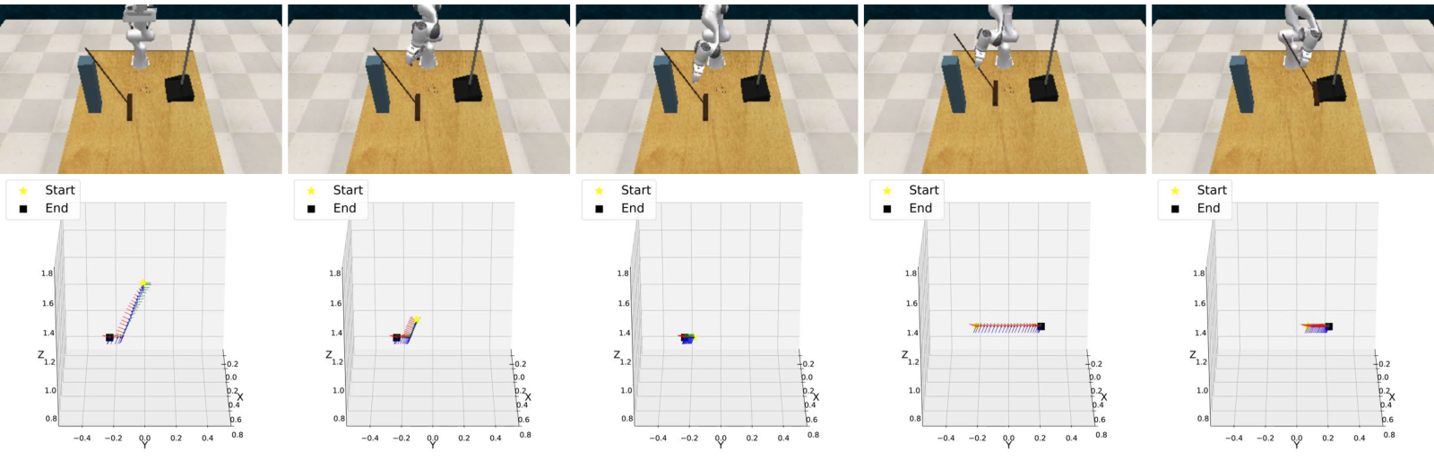
9 Task Details
9.1 RLBench Tasks
The full task names, descriptions, and number of corresponding keyposes of the selected 10 RLBench tasks are as follows:
(1) Sweep Dust (sweep to dustpan): use the broom to brush the dirt into the dustpan. This task involves 2 to 3 keyposes.
(2) Push Button (push button): press the button with the maroon base. This task involves 2 keyposes.
(3) Stack Wine (stack wine): slide the bottle onto the wine rack. This task involves 2 keyposes.
(4) Turn Tap (turn tap): grasp the tap and turn it. This task involves 2 keyposes.
(5) Open Drawer (open drawer): grip the bottom handle and pull the drawer open. This task involves 2 keyposes.
(6) Pick Up Cup (pick up cup): grasp the red cup and lift it. This task involves 2 keyposes.
(7) Take Lid (take lid off saucepan): using the handle, lift the lid off of the pan. This task involves 2 keyposes.
(8) Press Switch (press switch): turn the switch on or off. This task involves 2 keyposes.
(9) Reach Target (reach target): touch the red ball with the panda gripper. This task involves only 1 keypose.
(10) Open Box (open box): open the box lid. This task involves 2 keyposes.
9.2 RoboMimic Tasks
Descriptions and number of corresponding keyposes of three tasks from RoboMimic are as follows:
(1) Lift: grasp the cube from the table. This task involves 2 keyposes.
(2) Can: grasp the can and then place it in the designated place. This task involves 3 keyposes.
(3) Square: pick up the square and assemble it with the wooden peg. This task involves 3 keyposes.

9.3 Real-World Tasks
The visualization of the process of all real-world tasks can be found in Fig. 12, and the detailed descriptions are as follows:
(1) Cube: Grasping and placing a cube onto a plate. Demonstrations were collected in a specific area to test the ability to handle position changes in the workspace.
(2) Flip Cup: Grasping an inverted cup, flipping it mid-air, and placing it. The initial handle orientation was randomized to test complex 6-DoF manipulation.
(3) Package: Placing a cardboard into a box. Two distinct sets of demonstrations (10 samples each) were provided to evaluate the policy’s ability to handle multi-modality in action distributions.
(4) Banana: Picking up a banana. The pose of the banana is actively perturbed during execution to test real-time adaptation to dynamic scenarios.
(5) Screw Cap: Grasping a cap and screwing it onto a bottle. The initial position of the cap is randomized to test proficiency in high-precision operations.
10 Hyperparameters and Experiment Settings
RLBench We provide the training and evaluation hyperparameters for SegDiff and DP used on RLBench. The hyperparameters are aligned with previous works [52, 38, 9], allowing us to isolate and assess the impact of our proposed Segmented Trajectory Modeling. Specifically, SegDiff inherits most of its settings from DP. Additionally, we incorporate vanilla temporal ensembling into DP to ensure fair comparison.
RoboMimic We evaluate SegDiff against DP and AWE on the selected three RoboMimic tasks. The hyperparameters are shown in Tab. 8.
| Parameter | SegDiff | DP |
| Action dimension | 8 | 8 |
| Cameras | 4 | 4 |
| Image size | ||
| Observation horizon | 1 | 1 |
| Action sequence length | — | 20 |
| Interpolation length () | 25 | — |
| Batch size | 128 | 128 |
| Learning rate | ||
| Weight decay | ||
| Iteration | 100000 | 100000 |
| Hidden dim | 256 | 256 |
| Feedforward dim | 1024 | 1024 |
| Noise predictor | Transformer | Transformer |
| Scheduler | DDPM | DDPM |
| Train diffusion steps | 50 | 50 |
| Inference&Execution Parameters | ||
| Num. execution () | 1 | 1 |
| Update factor () | 0.25 | — |
| Threshold () | max | — |
| Sampling steps () | 50 | 50 |
| Inversion steps () | 10 | — |
| Parameter | SegDiff | DP | AWE |
| Action dimension | 8 | 8 | 8 |
| Cameras | 2 | 2 | 2 |
| Image size | |||
| Observation history | 2 | 2 | 2 |
| Horizon | — | 10 | 10 |
| Action sequence length | — | 8 | 8 |
| Interpolation length | 50 | — | — |
| Batch size | 64 | 64 | 64 |
| Learning rate | |||
| Weight decay | |||
| Epoch | 2000 | 2000 | 2000 |
| Hidden dim | 256 | 256 | 256 |
| Feedforward dim | 1024 | 1024 | 1024 |
| Noise predictor | Transformer | Transformer | Transformer |
| Noise scheduler | DDPM | DDPM | DDPM |
| Train diffusion steps | 100 | 100 | 100 |
| Inference & Execution Parameters | |||
| Num. execution () | 1 | — | — |
| Update factor () | 0.25 | — | — |
| Threshold () | max | — | — |
| Sampling steps () | 100 | 100 | 100 |
| Inversion steps () | 10 | — | — |
| Sweep Dust | Push Button | Stack Wine | Turn Tap | Open Drawer | Pick Up Cup | Take Lid | Press Switch | Reach Target | Open Box | |
| 0.025 | 0.109 | 0.099 | 0.125 | 0.121 | 0.036 | 0.063 | 0.148 | 0.034 | 0.024 | |
| 0.016 | 0.058 | 0.049 | 0.072 | 0.039 | 0.024 | 0.029 | 0.107 | 0.028 | 0.017 | |
| 0.012 | 0.037 | 0.028 | 0.048 | 0.024 | 0.017 | 0.015 | 0.085 | 0.023 | 0.014 |
11 Additional Experiment Results
11.1 DTE Threshold Analysis
A significant component of our Dynamic Temporal Ensembling (DTE) mechanism is the threshold , which is employed to determine whether two trajectories still belong to the same behavioral mode. This determination is crucial for assessing the validity of the actions within the buffer.
To estimate an effective value for , we operate on the fundamental assumption that all original trajectories in the training dataset represent correct behaviors conditioned on the given observation. Consequently, the reconstructed trajectory, obtained via DDIM inversion and subsequent sampling, should also belong to the same mode as the original. We statistically estimate the distribution of distances between these reconstructed and original trajectories to establish a quantitative baseline for "same-mode" proximity. While this estimation method based on reconstruction distance is inherently an approximation of the true mode distribution, it provides a measurable proxy.
The DTE mechanism exhibits robustness to the selection of the threshold ; detailed ablation results in Tab.10 confirm that the specific choice of does not significantly impact the final task success rate on RLBench.
The results calculated from the reconstruction distance distribution are shown in Tab.9 and the visualization of the reconstruction distance distribution is shown in Fig.13
| Method | Sweep Dust | Push Button | Stack Wine | Turn Tap | Open Drawer | Pick Up Cup | Take Lid | Press Switch | Reach Target | Open Box | Avg. |
| SegDiff | 0.96 | 0.76 | 0.88 | 0.72 | 1.00 | 0.96 | 0.80 | 0.80 | 1.00 | 0.72 | 0.860 |
| 1.00 | 0.92 | 0.96 | 0.84 | 1.00 | 0.92 | 0.92 | 0.72 | 0.96 | 0.56 | 0.880 | |
| 1.00 | 0.88 | 0.80 | 0.60 | 0.88 | 0.60 | 0.88 | 0.76 | 0.96 | 0.64 | 0.800 | |
| (w/o DTE) | 0.96 | 0.72 | 0.96 | 0.72 | 0.96 | 0.84 | 0.76 | 0.84 | 1.00 | 0.60 | 0.836 |
| (w/o DTE) | 1.00 | 0.88 | 0.92 | 0.72 | 0.92 | 0.88 | 0.88 | 0.76 | 0.96 | 0.84 | 0.876 |
| (w/o DTE) | 1.00 | 0.76 | 0.96 | 0.60 | 0.80 | 0.92 | 0.88 | 0.52 | 0.96 | 0.56 | 0.796 |
| 0.96 | 0.84 | 0.88 | 0.68 | 1.00 | 0.96 | 0.80 | 0.80 | 0.96 | 0.60 | 0.848 | |
| 0.92 | 0.76 | 0.88 | 0.72 | 0.96 | 0.84 | 0.80 | 0.72 | 1.00 | 0.76 | 0.836 | |
| 0.92 | 0.80 | 0.92 | 0.76 | 0.72 | 0.96 | 0.80 | 0.76 | 1.00 | 0.88 | 0.852 | |
| 0.96 | 0.76 | 0.88 | 0.64 | 1.00 | 0.96 | 0.84 | 0.84 | 1.00 | 0.72 | 0.860 | |
| 0.96 | 0.76 | 0.92 | 0.48 | 0.92 | 0.84 | 0.84 | 0.36 | 1.00 | 0.56 | 0.764 | |
| 0.28 | 0.84 | 0.76 | 0.56 | 0.64 | 0.84 | 0.68 | 0.72 | 1.00 | 0.48 | 0.680 | |
| 1.00 | 0.88 | 0.80 | 0.56 | 0.96 | 0.76 | 0.88 | 0.84 | 0.96 | 0.60 | 0.824 | |
| 0.84 | 0.76 | 0.76 | 0.60 | 1.00 | 0.76 | 0.84 | 0.88 | 0.96 | 0.60 | 0.800 | |
| 1.00 | 0.88 | 0.96 | 0.76 | 1.00 | 0.92 | 0.80 | 0.68 | 0.96 | 0.60 | 0.856 |
11.2 Detailed Ablation Results
We also study the effect of different interpolation methods. For rotation, we use spherical linear interpolation. For translation, we test both linear and cubic interpolation during training and evaluation. The results, together with those from ablation experiments on 10 RLBench tasks, are shown in Tab. 10. We test different Interpolation Lengths without Dynamic Temporal Ensembling (w/o DTE). and are defined in the experiment section to test the effect of introducing DDIM inversion. We also test the mode switch threshold , and the update factor used for blending trajectories. Additionally, we test the efficiency trade-off using different numbers of inversion steps () and sampling steps (). Finally, uses linear interpolation for translation compared to the default cubic interpolation.

12 Per-Task Results
For completeness, we report the detailed success rates for all RLBench-60 tasks in Tab. 11 and all RoboMimic settings in Tab. 12. These results correspond to the aggregated metrics presented in the main paper and provide a more fine-grained comparison across tasks.
| Simplified name | Full name | DP | CoA | SegDiff |
|---|---|---|---|---|
| lamp on | lamp_on | 0.00 | 0.48 | 0.80 |
| remove plate | take_plate_off_colored_dish_rack | 0.12 | 0.40 | 0.80 |
| pick up cup | pick_up_cup | 0.00 | 0.80 | 0.92 |
| reach target | reach_target | 0.08 | 0.84 | 0.96 |
| push button | push_button | 0.12 | 0.76 | 0.92 |
| open grill | open_grill | 0.00 | 0.24 | 0.56 |
| hang frame | hang_frame_on_hanger | 0.00 | 0.16 | 0.52 |
| lamp off | lamp_off | 0.20 | 0.68 | 0.88 |
| drag to target | reach_and_drag | 0.28 | 0.64 | 0.88 |
| turn tap | turn_tap | 0.32 | 0.56 | 0.84 |
| remove toilet roll | take_toilet_roll_off_stand | 0.08 | 0.56 | 0.72 |
| turn oven on | turn_oven_on | 0.28 | 0.36 | 0.72 |
| place plate | put_plate_in_colored_dish_rack | 0.04 | 0.32 | 0.56 |
| move hanger | move_hanger | 0.32 | 0.88 | 0.96 |
| open drawer | open_drawer | 0.44 | 0.88 | 1.00 |
| phone on base | phone_on_base | 0.04 | 0.80 | 0.76 |
| unplug charger | unplug_charger | 0.20 | 0.60 | 0.68 |
| take out shoes | take_shoes_out_of_box | 0.16 | 0.08 | 0.40 |
| remove frame | take_frame_off_hanger | 0.24 | 0.64 | 0.72 |
| stack wine | stack_wine | 0.56 | 0.80 | 0.96 |
| get ice | get_ice_from_fridge | 0.24 | 0.60 | 0.68 |
| place knife | place_knife_on_chopping_board | 0.00 | 0.04 | 0.28 |
| open wine | open_wine_bottle | 0.40 | 0.36 | 0.64 |
| slide block | slide_block_to_target | 0.00 | 0.52 | 0.52 |
| put bottle in fridge | put_bottle_in_fridge | 0.00 | 0.28 | 0.40 |
| close grill | close_grill | 0.68 | 0.56 | 0.88 |
| open box | open_box | 0.32 | 0.32 | 0.56 |
| hang hanger | place_hanger_on_rack | 0.00 | 0.32 | 0.40 |
| remove meat | meat_off_grill | 0.16 | 0.88 | 0.76 |
| open door | open_door | 0.60 | 0.92 | 1.00 |
| remove pan lid | take_lid_off_saucepan | 0.60 | 0.80 | 0.92 |
| remove umbrella | take_umbrella_out_of _umbrella_stand | 0.20 | 0.52 | 0.56 |
| put money in safe | put_money_in_safe | 0.24 | 0.80 | 0.72 |
| press switch | press_switch | 0.56 | 0.44 | 0.68 |
| water plants | water_plants | 0.00 | 0.48 | 0.40 |
| remove from scale | take_off_weighing_scales | 0.64 | 0.84 | 0.88 |
| play jenga | play_jenga | 0.72 | 1.00 | 1.00 |
| close box | close_box | 0.76 | 1.00 | 1.00 |
| screw nail | screw_nail | 0.00 | 0.08 | 0.16 |
| open microwave | open_microwave | 0.40 | 0.44 | 0.52 |
| set clock | change_clock | 0.20 | 0.40 | 0.40 |
| take out money | take_money_out_safe | 0.68 | 0.76 | 0.80 |
| hockey | hockey | 0.00 | 0.08 | 0.12 |
| close drawer | close_drawer | 0.76 | 1.00 | 0.96 |
| basketball | basketball_in_hoop | 0.72 | 0.76 | 0.80 |
| seat down | toilet_seat_down | 0.88 | 1.00 | 1.00 |
| put groceries on | put_groceries_in_cupboard | 0.00 | 0.08 | 0.08 |
| hit ball | hit_ball_with_cue | 0.00 | 0.08 | 0.08 |
| sweep dust | sweep_to_dustpan | 1.00 | 0.92 | 1.00 |
| buzz game | beat_the_buzz | 0.00 | 0.36 | 0.20 |
| change channel | change_channel | 0.00 | 0.12 | 0.08 |
| straighten rope | straighten_rope | 0.00 | 0.00 | 0.00 |
| close fridge | close_fridge | 0.76 | 0.92 | 0.84 |
| open washer | open_washing_machine | 0.60 | 0.76 | 0.64 |
| set checkers | setup_checkers | 0.04 | 0.04 | 0.00 |
| lift block | lift_numbered_block | 0.08 | 0.08 | 0.04 |
| remove USB | take_usb_out_of_computer | 0.72 | 0.60 | 0.60 |
| insert USB | insert_usb_in_computer | 0.88 | 0.92 | 0.84 |
| seat up | toilet_seat_up | 0.88 | 0.84 | 0.76 |
| Demos | Task | DP | AWE | SegDiff |
| Lift | 1.00 | 1.00 | 1.00 | |
| 30 | Can | 0.64 | 0.62 | 0.66 |
| Square | 0.42 | 0.36 | 0.44 | |
| Lift | 1.00 | 1.00 | 1.00 | |
| 50 | Can | 0.86 | 0.77 | 0.87 |
| Square | 0.52 | 0.49 | 0.55 | |
| Lift | 1.00 | 1.00 | 1.00 | |
| 100 | Can | 0.93 | 0.87 | 0.92 |
| Square | 0.78 | 0.77 | 0.78 | |
| Lift | 1.00 | 1.00 | 1.00 | |
| 200 | Can | 0.98 | 0.96 | 0.98 |
| Square | 0.94 | 0.88 | 0.92 |
