跳到论文正文
W Papers独立论文阅读器 arXiv:2607.08157 论文正文 计算阅读时间 · 0%
引用这篇论文根据当前论文元数据生成,正式投稿前建议核对。


License: arXiv.org perpetual non-exclusive license
arXiv:2607.08157v1 [math.ST] 09 Jul 2026

Parameter inference for
partially observed branching processes

Simone Baldassarri Gran Sasso Science Institute, Viale Francesco Crispi 7, 67100 L’Aquila, Italy. simone.baldassarri@gssi.it , Michel Mandjes Mathematical Institute, Leiden University, P.O. Box 9512, 2300 RA Leiden, The Netherlands. m.r.h.mandjes@math.leidenuniv.nl and Jiesen Wang Korteweg-de Vries Institute for Mathematics, University of Amsterdam, Science Park 105-107, 1098 XG Amsterdam, The Netherlands. jiesenwang@gmail.com
Abstract.

In this paper, we study an age-dependent branching process. In the simplest setting, the population is divided into two age groups, namely juveniles and adults. Our objective is to estimate the model parameters using observations of the total population size only (i.e., juveniles plus adults). Focusing on the ergodic regime of the model, we introduce a method-of-moments estimator and establish its asymptotic normality. Several extensions are discussed, including models with more than two age groups.

Keywords. Age-dependent branching process, partial information, parametric inference, method of moments.

Acknowledgments. This research was supported by the European Union’s Horizon 2020 research and innovation programme under the Marie Skłodowska-Curie grant agreement no. 945045, and by the NWO Gravitation project NETWORKS under grant agreement no. 024.002.003. SB was further supported through “Gruppo Nazionale per l’Analisi Matematica, la Probabilità e le loro Applicazioni” (GNAMPA-INdAM).

1. Introduction

In this paper we consider a branching process with two age groups [2], namely juveniles (Xn)n≥0(X_{n})_{n\geq 0} and adults (Yn)n≥0(Y_{n})_{n\geq 0}, where XnX_{n} and YnY_{n} denote the population sizes in this first and second age class at generation nn, respectively. The main objective of this paper is to estimate the underlying parameters of the process. In many practical situations, however, only the aggregate population size

Zn:=Xn+YnZ_{n}:=X_{n}+Y_{n}

is observed. This presents a non-standard scenario for modeling and inference, as the observed data is aggregated, and the age structure is hidden. Observe that the bivariate process (Xn,Yn)n≥0(X_{n},Y_{n})_{n\geq 0} is Markovian, but that the aggregated process (Zn)n≥0(Z_{n})_{n\geq 0} is not, which poses significant challenges for standard inference techniques.

The proposed estimation procedure is based on the method of moments [7, 19]. Specifically, we derive explicit expressions for moments of the observable sequence (Zn)n≥0(Z_{n})_{n\geq 0} as functions of the underlying (unknown) model parameters. These theoretical moments are then equated to their empirical counterparts computed from the data, and the resulting system of equations is solved to obtain estimators for the unknown parameters. For clarity of exposition, we first present the approach in the elementary setting with two age groups and immigration into one of them. We subsequently indicate how the methodology extends in a natural way to models with an arbitrary number of age groups, with immigration occurring in any subset of these groups, as well as to settings in which the reproduction mechanism is more general.

We now proceed by outlining the main results of the paper. Restricting attention to the ergodic regime, we first introduce our estimator and establish that the associated system of moment equations admits a unique solution, thereby ensuring well-definedness of the procedure. As a next step, we show that the empirical moment vector is asymptotically multivariate normal as the number of observations NN tends to infinity. Building on this result, we invoke the delta-method [24] to deduce that the proposed estimator itself is asymptotically multivariate normal. Finally, we derive explicit expressions for the entries of the corresponding covariance matrix, expressed directly in terms of the model primitives.

The proposed procedure is evaluated through a series of numerical experiments designed to assess its finite-sample performance. The results indicate that the estimator performs accurately across a range of parameter settings.

We also discuss several extensions of the basic framework. In particular, we consider observation schemes in which only one of the age groups is observed. Another extension concerns models with more than two age groups, where each adult group may reproduce and immigration may occur in any of the groups. We argue that the estimation methodology extends in a conceptually straightforward manner to this more general setting, although the resulting expressions and computations become substantially more involved.

Various techniques for handling unobserved or latent quantities have been developed in the mathematical statistics literature. In the present setting, however, their application is far from straightforward.

Likelihood-based methods are difficult to implement in this setting. Evaluating the likelihood would require either full observation of the age structure or an explicit characterization of the transition dynamics of the non-Markovian process (Zn)n≥0(Z_{n})_{n\geq 0}, which depend on the unobserved population composition. This naturally leads to formulations in terms of hidden or partially observed Markov processes [5], for which likelihood evaluation and optimization are often analytically intractable and computationally intensive, especially when the state space is large or the time series is short. Numerical implementations also typically rely on simulation-based procedures, which can be sensitive to tuning and initialization. By contrast, the method-of-moments approach adopted here avoids likelihood evaluation altogether. By exploiting explicit relationships between observable moments of (Zn)n≥0(Z_{n})_{n\geq 0} and the underlying parameters, it circumvents the need to reconstruct the latent age structure and yields estimators that are computationally transparent, scalable, and well suited to aggregated population data.

Expectation-Maximization (EM)-type algorithms might appear to offer a principled alternative [10, 19], given the latent structure of the model. However, their application here is also problematic. The E-step requires computing conditional expectations with respect to the smoothing distribution of the latent process (Xn,Yn)n≥0(X_{n},Y_{n})_{n\geq 0} given only observations of (Zn)n≥0(Z_{n})_{n\geq 0}. Because the observed process lacks the Markov property, this smoothing distribution does not admit a simple recursive representation. As a result, EM implementations would necessarily rely on numerical or simulation-based approximations, leading to high computational cost. Moreover, the aggregation inherent in (Zn)n≥0(Z_{n})_{n\geq 0} may induce weak identifiability, causing slow convergence or sensitivity to initialization.

Simulation-based approaches, such as particle filters or approximate Bayesian computation (ABC), face similar difficulties in this setting. These methods require repeated simulation of the latent age-structured process and careful tuning of algorithmic parameters, and their performance can degrade substantially when inference is based solely on aggregated observations. For a detailed discussion of particle filtering and sequential Monte Carlo methods, see e.g. [6, 11], and for ABC techniques, see e.g. [4, 23]. These references highlight both the computational cost and the sensitivity of such methods to tuning and initialization, illustrating why direct likelihood-free approaches, such as the method-of-moments, may be preferable when only aggregated data (Zn)n≥0(Z_{n})_{n\geq 0} are available.

By contrast, the method-of-moments approach developed here directly exploits explicit relationships between the observable moments of (Zn)n≥0(Z_{n})_{n\geq 0} and the underlying model parameters. This strategy avoids likelihood evaluation altogether and bypasses the need to reconstruct the hidden age structure. As a result, the proposed estimators are computationally simple, scalable, and robust to the non-Markovian nature of the observed process, making them particularly attractive in settings where only aggregate population data are available.

In the literature on structured population models it is often suggested that parameters governing stage- or age-structured population dynamics cannot be uniquely identified when only aggregate population counts are observed. The intuition behind this concern is that different combinations of reproduction, maturation, and immigration parameters may generate probabilistically identical trajectories for the total population size, making it difficult to disentangle the underlying mechanisms without observing the individual stages. In practice, statistical analyses of structured population models typically rely on stage-specific observations; see, for instance, the classical treatment in [8]. Related inference problems also arise in the study of branching processes, where the statistical analysis generally assumes that the different types or generations can be observed separately; see [14]. The results obtained in this paper show that, for the stochastic juvenile-adult branching model with immigration considered here, the key parameters can in fact be uniquely identified from the time series of the total population size alone. In particular, under the Poisson assumptions for immigration and reproduction, the parameters governing immigration, juvenile maturation, and adult reproduction can be consistently estimated from aggregate observations.

In a broader sense, the scope of this paper lies within what could be called the area of ‘statistics for stochastic processes’. Such problems can be viewed as instances of inverse problems, in which the objective is to infer underlying model parameters from limited, indirect, or aggregated data. In the statistics and applied probability literature, a wide range of inverse problems has been studied. A classical example is the estimation of the offspring distribution in a Galton-Watson branching process from longitudinal population data; see, for instance, the textbook [14]. In epidemiology, one seeks to estimate the parameters of a stochastic SIR model based on observed infection counts over time [9]. Related inverse problems arise in finance [1, 12] and in queueing theory [13, 16, 22]. More recently, attention has turned to the estimation of random graph dynamics from partial observations. For example, [20] considers a dynamic Erdős-Rényi graph in which edges randomly alternate between presence and absence, with inference based on observed subgraph counts, [15] extends the analysis to the dynamic Chung-Lu graph, and [3] addresses the problem for a voter model evolving on a dynamic Erdős-Rényi graph.

The remainder of the paper is organized as follows. In Section 2, we introduce the age-dependent branching model and present the proposed method-of-moments estimator. Section 3 is devoted to the proof of its asymptotic normality. In Section 4, we discuss two extensions of the basic framework, namely alternative observation schemes and models with more than two age groups. Finally, Section 5 concludes the paper with a brief discussion of the results and several directions for future research.

2. Model and estimator

In the first part of this paper, we consider a setting in which the population consists of two types, namely juveniles and adults. Although this simplified structure may not be entirely realistic, it provides a convenient and transparent framework for illustrating the construction of our estimator and for establishing its asymptotic normality. We emphasize, however, that this restriction is not essential: in Section 4 we show that the methodology developed here extends naturally to substantially more general and realistic age-dependent branching processes.

In the specific setting considered in this section and in Section 3, reproduction occurs only among adults. Each adult produces a random number of juveniles (often referred to as ‘offspring’). Juveniles require one time step to mature into adults, provided they survive; that is, offspring face a positive probability of dying before reaching adulthood. Adults live for exactly one time unit. In addition, at each generation there is an immigration component, introducing new juveniles into the population, thus helping to prevent extinction. The usual independence assumptions are imposed. Finally, we assume a condition ensuring that the population does not explode; this condition is identified below.

2.1. Model description, observation scheme

Let XnX_{n} denote the number of juveniles and YnY_{n} the number of adults in timeslot nn, respectively. The variable XnX_{n} is updated based on an exogenous input InI_{n} and a sum of random contributions from Yn−1Y_{n-1}, while YnY_{n} evolves via a binomial thinning of Xn−1X_{n-1}. This means that, formally, the dynamics are given by

Xn+1=In+∑i=1YnGn,i,Yn+1∼Bin​(Xn,p),X_{n+1}=I_{n}+\sum_{i=1}^{Y_{n}}G_{n,i},\qquad Y_{n+1}\sim\text{Bin}(X_{n},p), (2.1)

where {In}n≥0\{I_{n}\}_{n\geq 0} is a sequence of i.i.d. input variables that are distributed as the generic random variable I∈ℕ0I\in{\mathbb{N}}_{0}, and {Gn,i}n,i≥1\{G_{n,i}\}_{n,i\geq 1} are i.i.d. random variables distributed as the generic random variable G∈ℕ0G\in{\mathbb{N}}_{0}, independent of {In}n≥0\{I_{n}\}_{n\geq 0}. The model dynamics are illustrated in Figure 1.

The objective is to estimate pp and the parameters associated with II and GG from observations. If II and GG belong to one-parameter families with unknown parameters λ\lambda and ν\nu, respectively, and pp is an additional unknown parameter, then the parameter vector to be estimated is 𝜽≡(p,λ,ν){\boldsymbol{\theta}}\equiv(p,\lambda,\nu). The main complication is that we do not observe the individual components {Xn}n≥0\{X_{n}\}_{n\geq 0} and {Yn}n≥0\{Y_{n}\}_{n\geq 0}, but only the total population. That is, the observable process is {Zn}n≥0\{Z_{n}\}_{n\geq 0}, where

Zn:=Xn+Yn.Z_{n}:=X_{n}+Y_{n}.

Importantly, while the pair (Xn,Yn)(X_{n},Y_{n}) is Markovian, the process {Zn}n≥0\{Z_{n}\}_{n\geq 0} alone is not.

It is noted that, while in the next section we focus on constructing an estimator for 𝜽{\boldsymbol{\theta}} in the case where the total population is observed, the proposed methodology also applies (with a minor modification) when only the juvenile population {Xn}n≥0\{X_{n}\}_{n\geq 0} is observed; see the discussion in Section 4. Remarkably, in that same section we also argue that 𝜽{\boldsymbol{\theta}} cannot be estimated when only the adult population {Yn}n≥0\{Y_{n}\}_{n\geq 0} is observed.

Y1Y_{1}X2X_{2}Y3Y_{3}X4X_{4}X1X_{1}Y2Y_{2}X3X_{3}Y4Y_{4}†{\dagger}†{\dagger}†{\dagger}†{\dagger}†{\dagger}
Figure 1. Illustration of the evolution of the populations XnX_{n} and YnY_{n} for n=1,…,4n=1,\ldots,4. (a) Grey-shaded individuals represent immigrants in each generation, with counts I1=1I_{1}=1, I2=0I_{2}=0, I3=2I_{3}=2, and I4=1I_{4}=1. (b) In the boxes XnX_{n}, a dagger (†\dagger) next to an individual indicates that it ‘dies’, meaning it does not survive to become a member of Yn+1Y_{n+1}. In contrast, arrows connecting individuals in XnX_{n} to Yn+1Y_{n+1} represent juveniles that successfully mature into adults. (c) Arrows from YnY_{n} to Xn+1X_{n+1} depict the offspring produced by members of YnY_{n}. For example, G3,2=3G_{3,2}=3 indicates that the second member of Y3Y_{3} produces three offspring in X4X_{4}; in our sample path, we also have G1,1=1G_{1,1}=1, G1,2=2G_{1,2}=2, G2,1=0G_{2,1}=0, and G3,1=1G_{3,1}=1. Overall, the figure visualizes the generational dynamics, covering survival, reproduction, and immigration events.

The process {Xn,Yn}n≥0\{X_{n},Y_{n}\}_{n\geq 0} is clearly Markovian. As we will establish below, the process is ergodic under the stability condition

ϱ:=p​𝔼​[G]<1.\varrho:=p\,\mathbb{E}[G]<1. (S)

Throughout this paper, we specifically pay attention to the case that the random variables II and GG have Poisson distributions:

I∼Poisson​(λ),G∼Poisson​(ν).I\sim{\rm Poisson}(\lambda),\quad G\sim{\rm Poisson}(\nu). (P)

2.2. Estimator

We consider the convenient situation that the process {Xn,Yn}n≥0\{X_{n},Y_{n}\}_{n\geq 0} is ergodic, and that we start in stationarity. Suppose that the moments we target are

𝒎≡(m1,m2,m12):=(𝔼​[Zn],𝔼​[Zn2],𝔼​[Zn+1​Zn]),{\boldsymbol{m}}\equiv(m_{1},m_{2},m_{12}):=\bigl(\mathbb{E}[Z_{n}],\ \mathbb{E}[Z_{n}^{2}],\ \mathbb{E}[Z_{n+1}Z_{n}]\bigr),

which, by our assumptions, do not depend on nn. Given observations Z1,…,ZNZ_{1},\dots,Z_{N} for some N≥2N\geq 2, the corresponding empirical moments are 𝒎^N≡(m^1,N,m^2,N,m^12,N)\hat{\boldsymbol{m}}_{N}\equiv(\hat{m}_{1,N},\hat{m}_{2,N},\hat{m}_{12,N}), with

m^1,N=1N​∑n=1NZn,m^2,N=1N​∑n=1NZn2,m^12,N=1N−1​∑n=1N−1Zn+1​Zn,\hat{m}_{1,N}=\frac{1}{N}\sum_{n=1}^{N}Z_{n},\qquad\hat{m}_{2,N}=\frac{1}{N}\sum_{n=1}^{N}Z_{n}^{2},\qquad\hat{m}_{12,N}=\frac{1}{N-1}\sum_{n=1}^{N-1}Z_{n+1}Z_{n},

respectively. The method-of-moments estimators (p^N,λ^I,N,λ^G,N)(\hat{p}_{N},\hat{\lambda}_{I,N},\hat{\lambda}_{G,N}) are then obtained by solving the following three equations with three unknowns:

(𝔼​[Zn],𝔼​[Zn2],𝔼​[Zn+1​Zn])=(m^1,N,m^2,N,m^12,N),\bigl(\mathbb{E}[Z_{n}],\ \mathbb{E}[Z_{n}^{2}],\ \mathbb{E}[Z_{n+1}Z_{n}]\bigr)=\bigl(\hat{m}_{1,N},\ \hat{m}_{2,N},\ \hat{m}_{12,N}\bigr),

where it is observed that the left-hand side consists of functions of entries of 𝜽{\boldsymbol{\theta}}. Below we demonstrate this approach by detailing the three steps: (a) deriving expressions for the moments, (b) expressing the moments in terms of the unknown parameters 𝜽{\boldsymbol{\theta}}, (c) solving the moment equations, thus rendering our estimators. When setting up these estimators, we assume that II and GG have finite second moments.

  • (a)

    We derive expressions for 𝔼​[Zn]\mathbb{E}[Z_{n}], 𝔼​[Zn2]\mathbb{E}[Z_{n}^{2}], and 𝔼​[Zn+1​Zn]\mathbb{E}[Z_{n+1}Z_{n}]. Using the identity Zn=Xn+YnZ_{n}=X_{n}+Y_{n}, we obviously have, for any nn,

    𝔼​[Zn]\displaystyle\mathbb{E}[Z_{n}] =𝔼​[Xn]+𝔼​[Yn],\displaystyle=\mathbb{E}[X_{n}]+\mathbb{E}[Y_{n}], (2.2)
    𝔼​[Zn2]\displaystyle\mathbb{E}[Z_{n}^{2}] =𝔼​[Xn2]+2​𝔼​[Xn​Yn]+𝔼​[Yn2],\displaystyle=\mathbb{E}[X_{n}^{2}]+2\,\mathbb{E}[X_{n}Y_{n}]+\mathbb{E}[Y_{n}^{2}], (2.3)
    𝔼​[Zn+1​Zn]\displaystyle\mathbb{E}[Z_{n+1}Z_{n}] =𝔼​[Xn+1​Xn]+𝔼​[Xn+1​Yn]+𝔼​[Yn+1​Xn]+𝔼​[Yn+1​Yn].\displaystyle=\mathbb{E}[X_{n+1}X_{n}]+\mathbb{E}[X_{n+1}Y_{n}]+\mathbb{E}[Y_{n+1}X_{n}]+\mathbb{E}[Y_{n+1}Y_{n}]. (2.4)

    Using the model dynamics (2.1) and Wald’s equation, this last expression can be rewritten as

    𝔼​[Zn+1​Zn]\displaystyle\mathbb{E}[Z_{n+1}Z_{n}] =𝔼​[I]​𝔼​[Xn]+𝔼​[G]​𝔼​[Xn​Yn]+𝔼​[I]​𝔼​[Yn]+𝔼​[G]​𝔼​[Yn2]\displaystyle=\mathbb{E}[I]\,\mathbb{E}[X_{n}]+\mathbb{E}[G]\,\mathbb{E}[X_{n}Y_{n}]+\mathbb{E}[I]\,\mathbb{E}[Y_{n}]+\mathbb{E}[G]\,\mathbb{E}[Y_{n}^{2}]
    +p​𝔼​[Xn​Yn]+p​𝔼​[Xn2].\displaystyle\quad+p\,\mathbb{E}[X_{n}Y_{n}]+p\,\mathbb{E}[X_{n}^{2}]. (2.5)

    Consequently, it suffices to derive expressions for the five quantities

    𝔼​[Xn],𝔼​[Yn],𝔼​[Xn​Yn],𝔼​[Xn2],𝔼​[Yn2].\mathbb{E}[X_{n}],\quad\mathbb{E}[Y_{n}],\quad\mathbb{E}[X_{n}Y_{n}],\quad\mathbb{E}[X_{n}^{2}],\quad\mathbb{E}[Y_{n}^{2}].
  • (b)

    Observe that the only information about II and GG that we need in (2.5) is 𝔼​[I]\mathbb{E}[I] and 𝔼​[G]\mathbb{E}[G]. It is now straightforward to conclude that, again as an application of Wald’s equation, 𝔼​[Xn]=𝔼​[I]+𝔼​[G]​𝔼​[Yn−1]\mathbb{E}[X_{n}]=\mathbb{E}[I]+\mathbb{E}[G]\,\mathbb{E}[Y_{n-1}] and 𝔼​[Yn]=p​𝔼​[Xn−1]\mathbb{E}[Y_{n}]=p\,\mathbb{E}[X_{n-1}], confirming the stationarity condition ϱ:=p​𝔼​[G]<1\varrho:=p\,\mathbb{E}[G]<1 as given by (S). Thus, for any nn,

    𝔼​[Xn]\displaystyle\mathbb{E}[X_{n}] =𝔼​[I]1−p​𝔼​[G],𝔼​[Yn]=p​𝔼​[Xn]=p​𝔼​[I]1−p​𝔼​[G];\displaystyle=\frac{\mathbb{E}[I]}{1-p\,\mathbb{E}[G]},\qquad\mathbb{E}[Y_{n}]=p\,\mathbb{E}[X_{n}]=\frac{p\,\mathbb{E}[I]}{1-p\,\mathbb{E}[G]}; (2.6)

    these means (2.6) follow by using that in stationarity 𝔼​[Xn]=𝔼​[Xn+1]\mathbb{E}[X_{n}]=\mathbb{E}[X_{n+1}] and 𝔼​[Yn]=𝔼​[Yn+1]\mathbb{E}[Y_{n}]=\mathbb{E}[Y_{n+1}]. In addition, with 𝔽​[G,I]:=2​𝔼​[I]​𝔼​[G]+𝕍​ar​[G]{\mathbb{F}}[G,I]:=2\mathbb{E}[I]\,\mathbb{E}[G]+{\mathbb{V}}{\rm ar}[G], for any nn,

    𝔼​[Xn​Yn]\displaystyle\mathbb{E}[X_{n}Y_{n}] =p​𝔼​[I]​𝔼​[Xn]1−p​𝔼​[G]=p​𝔼​[I]2(1−p​𝔼​[G])2,\displaystyle=\frac{p\,\mathbb{E}[I]\,\mathbb{E}[X_{n}]}{1-p\,\mathbb{E}[G]}=\frac{p\,\mathbb{E}[I]^{2}}{(1-p\,\mathbb{E}[G])^{2}}, (2.7)
    (𝔼​[Xn2]𝔼​[Yn2])\displaystyle\left(\begin{array}[]{c}\mathbb{E}[X_{n}^{2}]\\ \mathbb{E}[Y_{n}^{2}]\end{array}\right) =(1−(𝔼​[G])2−p21)−1​(𝔽​[G,I]​𝔼​[Yn]+𝔼​[I2]p​(1−p)​𝔼​[Xn])\displaystyle=\left(\begin{array}[]{cc}1&-(\mathbb{E}[G])^{2}\\ -p^{2}&1\end{array}\right)^{-1}\left(\begin{array}[]{c}{\mathbb{F}}[G,I]\,\mathbb{E}[Y_{n}]+\mathbb{E}[I^{2}]\\ p(1-p)\,\mathbb{E}[X_{n}]\\ \end{array}\right) (2.14)
    =11−p2​𝔼​[G]2​(1𝔼​[G]2p21)​(𝔽​[G,I]​𝔼​[Yn]+𝔼​[I2]p​(1−p)​𝔼​[Xn]).\displaystyle=\dfrac{1}{1-p^{2}\mathbb{E}[G]^{2}}\left(\begin{array}[]{cc}1&\mathbb{E}[G]^{2}\\ p^{2}&1\end{array}\right)\left(\begin{array}[]{c}{\mathbb{F}}[G,I]\,\mathbb{E}[Y_{n}]+\mathbb{E}[I^{2}]\\ p(1-p)\,\mathbb{E}[X_{n}]\\ \end{array}\right). (2.19)

    The expression for 𝔼​[Xn​Yn]\mathbb{E}[X_{n}Y_{n}], as presented in (2.7), is found via a straightforward application of the tower property. Indeed, we observe

    𝔼​[Xn+1​Yn+1]\displaystyle\mathbb{E}[X_{n+1}Y_{n+1}] =𝔼​[𝔼​[(In+∑i=1YnGn,i)​Bin​(Xn,p)|Xn,Yn]]\displaystyle=\mathbb{E}\left[\mathbb{E}\left[\left(I_{n}+\sum_{i=1}^{Y_{n}}G_{n,i}\right){\rm Bin}(X_{n},p)\Big|X_{n},Y_{n}\right]\right]
    =𝔼​[(𝔼​[I]+Yn​𝔼​[G])​p​Xn]=p​𝔼​[I]​𝔼​[Xn]+p​𝔼​[G]​𝔼​[Xn​Yn].\displaystyle=\mathbb{E}\Big[\big(\mathbb{E}[I]+Y_{n}\,\mathbb{E}[G]\big)\,p\,X_{n}\Big]=p\,\mathbb{E}[I]\,\mathbb{E}[X_{n}]+p\,\mathbb{E}[G]\,\mathbb{E}[X_{n}Y_{n}].

    Then, using that in stationarity 𝔼​[Xn​Yn]=𝔼​[Xn+1​Yn+1]\mathbb{E}[X_{n}Y_{n}]=\mathbb{E}[X_{n+1}Y_{n+1}], and recalling the expression for 𝔼​[Xn]\mathbb{E}[X_{n}], the above expression for 𝔼​[Xn​Yn]\mathbb{E}[X_{n}Y_{n}] directly follows. (As an aside, we observe that our computation reveals that XnX_{n} and YnY_{n} are uncorrelated; via some additional computations we verified that they are actually not independent.) Along similar lines (2.19) was proven; the key intermediate step is to verify that

    (𝔼​[Xn+12]𝔼​[Yn+12])=((𝔼​[G])2​𝔼​[Yn2]p2​𝔼​[Xn2])+(𝔽​[G,I]​𝔼​[Yn]p​(1−p)​𝔼​[Xn])+(𝔼​[I2]0).\left(\begin{array}[]{c}\mathbb{E}[X_{n+1}^{2}]\\ \mathbb{E}[Y_{n+1}^{2}]\end{array}\right)=\left(\begin{array}[]{c}(\mathbb{E}[G])^{2}\,\mathbb{E}[Y_{n}^{2}]\\ p^{2}\mathbb{E}[X_{n}^{2}]\end{array}\right)+\left(\begin{array}[]{c}{\mathbb{F}}[G,I]\,\mathbb{E}[Y_{n}]\\ p(1-p)\,\mathbb{E}[X_{n}]\end{array}\right)+\left(\begin{array}[]{c}\mathbb{E}[I^{2}]\\ 0\end{array}\right).

    For the ‘Poisson case’, i.e., under (P), the above expressions can be evaluated somewhat more explicitly, using that λ=𝔼​[I]=𝕍​ar​[I]\lambda=\mathbb{E}[I]={\mathbb{V}}{\rm ar}[I] and ν=𝔼​[G]=𝕍​ar​[G]\nu=\mathbb{E}[G]={\mathbb{V}}{\rm ar}[G],

    𝔼​[Xn]\displaystyle\mathbb{E}[X_{n}] =λ1−p​ν,𝔼​[Yn]=λ​p1−p​ν,𝔼​[Xn​Yn]=λ2​p(1−p​ν)2,\displaystyle=\frac{\lambda}{1-p\,\nu},\qquad\mathbb{E}[Y_{n}]=\frac{\lambda p}{1-p\,\nu},\qquad\mathbb{E}[X_{n}Y_{n}]=\frac{\lambda^{2}p}{(1-p\,\nu)^{2}}, (2.20)
    𝔼​[Xn2]\displaystyle\mathbb{E}[X_{n}^{2}] =λ1−p​ν+λ2+λ​p​(ν2+2​λ​ν)/(1−p​ν)1−p2​ν2,\displaystyle=\frac{\lambda}{1-p\,\nu}+\frac{\lambda^{2}+\lambda p(\nu^{2}+2\lambda\nu)/(1-p\,\nu)}{1-p^{2}\,\nu^{2}}, (2.21)
    𝔼​[Yn2]\displaystyle\mathbb{E}[Y_{n}^{2}] =λ​p1−p​ν+p2​(λ2+λ​p​(ν2+2​λ​ν)/(1−p​ν))1−p2​ν2.\displaystyle=\frac{\lambda p}{1-p\,\nu}+\frac{p^{2}\bigl(\lambda^{2}+\lambda p(\nu^{2}+2\lambda\nu)/(1-p\,\nu)\bigr)}{1-p^{2}\,\nu^{2}}. (2.22)
  • (c)

    Combining these expressions with (2.2)–(2.5), we have succeeded in expressing the moment vector 𝒎≡(𝔼​[Zn],𝔼​[Zn2],𝔼​[Zn+1​Zn]){\boldsymbol{m}}\equiv(\mathbb{E}[Z_{n}],\mathbb{E}[Z_{n}^{2}],\mathbb{E}[Z_{n+1}Z_{n}]) in terms of the parameter 𝜽≡(p,λ,ν).{\boldsymbol{\theta}}\equiv(p,\lambda,\nu). We have thus identified a mapping F:ℝ3→ℝ3F:{\mathbb{R}}^{3}\to{\mathbb{R}}^{3} such that 𝒎=F​(𝜽){\boldsymbol{m}}=F({\boldsymbol{\theta}}). This leads to the estimator

    𝜽^N:=F−1​(𝒎^N).\hat{\boldsymbol{\theta}}_{N}:=F^{-1}(\hat{\boldsymbol{m}}_{N}).

We know discuss the well-definedness of the estimator 𝜽^N\hat{\boldsymbol{\theta}}_{N}. We consider the parameter space

Θ={(p,λ,ν):p∈(0,1),𝔼​[I]>0,𝔼​[G]>0,p​𝔼​[G]<1}.\Theta=\{(p,\lambda,\nu):p\in(0,1),\,\mathbb{E}[I]>0,\,\mathbb{E}[G]>0,\,p\,\mathbb{E}[G]<1\}.

To properly define 𝜽^N\hat{\boldsymbol{\theta}}_{N} as F−1​(𝒎^N)F^{-1}(\hat{\boldsymbol{m}}_{N}), we would like the following identifiability property to apply:

For any 𝒎∈ℝ+3{\boldsymbol{m}}\in{\mathbb{R}}_{+}^{3}, the equation 𝒎=F​(𝜽){\boldsymbol{m}}=F({\boldsymbol{\theta}}) has a unique solution in Θ\Theta. (U)

The following lemma shows that for Poissonian II and GG, under the stability condition ϱ=p​ν<1\varrho=p\,\nu<1, there is identifiability.

Lemma 2.1 (Identifiability).

Under assumptions (P) and (S), the identifiability condition (U) holds.

Proof. By direct computations, we can write

𝔼​[Zn2]−𝔼​[Zn]2\displaystyle\mathbb{E}[Z_{n}^{2}]-\mathbb{E}[Z_{n}]^{2} =λ​(1+p+p​(1−p)​ν2)(1−p​ν)2​(1+p​ν),\displaystyle=\dfrac{\lambda(1+p+p(1-p)\nu^{2})}{(1-p\nu)^{2}(1+p\nu)}, (2.23)
𝔼​[Zn+1​Zn]−𝔼​[Zn]2\displaystyle\mathbb{E}[Z_{n+1}Z_{n}]-\mathbb{E}[Z_{n}]^{2} =p​λ​(1+ν+p​(1−p)​ν2)(1−p​ν)2​(1+p​ν).\displaystyle=\dfrac{p\lambda(1+\nu+p(1-p)\nu^{2})}{(1-p\nu)^{2}(1+p\nu)}. (2.24)

Thus, by letting R:=(𝔼​[Zn+1​Zn]−𝔼​[Zn]2)/(𝔼​[Zn2]−𝔼​[Zn]2)R:=(\mathbb{E}[Z_{n+1}Z_{n}]-\mathbb{E}[Z_{n}]^{2})/(\mathbb{E}[Z_{n}^{2}]-\mathbb{E}[Z_{n}]^{2}),

𝔼​[Zn+1​Zn]−𝔼​[Zn]2𝔼​[Zn2]−𝔼​[Zn]2=p​(1+ν+p​(1−p)​ν2)1+p+p​(1−p)​ν2=:F(p,ν);\dfrac{\mathbb{E}[Z_{n+1}Z_{n}]-\mathbb{E}[Z_{n}]^{2}}{\mathbb{E}[Z_{n}^{2}]-\mathbb{E}[Z_{n}]^{2}}=\dfrac{p(1+\nu+p(1-p)\nu^{2})}{1+p+p(1-p)\nu^{2}}=:F(p,\nu);

observe that λ\lambda has canceled. Note that the function F​(p,ν)F(p,\nu) is strictly increasing in pp for any admissible ν>0\nu>0, namely, p​ν<1p\nu<1. Indeed, by a direct computation, ∂F/∂p\partial F/\partial p is positive if and only if

ν​[1+2​p​(1−p)​ν+p2​(p−1)2​ν3]+(1−p​ν)​(1+p​ν)>0,\nu[1+2p(1-p)\nu+p^{2}(p-1)^{2}\nu^{3}]+(1-p\nu)(1+p\nu)>0,

which is true for any θ∈Θ\theta\in\Theta. By arguing in a similar manner, we deduce that the function F​(p,ν)F(p,\nu) is strictly increasing in ν\nu for any admissible p∈(0,1)p\in(0,1). Thus, for any fixed pp, there exists a unique solution ν​(p)\nu(p) to the equation F​(p,ν​(p))=RF(p,\nu(p))=R, and from the implicit function theorem we have

d​ν​(p)d​p=−∂F/∂p∂F/∂ν<0.\dfrac{\mathrm{d}\nu(p)}{\mathrm{d}p}=-\dfrac{\partial F/\partial p}{\partial F/\partial\nu}<0.

This implies that the map p↦ν​(p)p\mapsto\nu(p) is monotonically decreasing.

Considering the ratio of 𝔼​[Zn2]−𝔼​[Zn]2\mathbb{E}[Z_{n}^{2}]-\mathbb{E}[Z_{n}]^{2} and 𝔼​[Zn]\mathbb{E}[Z_{n}], we observe that again λ\lambda cancels; from the equation

𝔼​[Zn2]−𝔼​[Zn]2𝔼​[Zn]=1+p+p​(1−p)​ν​(p)21−p2​ν​(p)2=:G(p,ν(p)),\dfrac{\mathbb{E}[Z_{n}^{2}]-\mathbb{E}[Z_{n}]^{2}}{\mathbb{E}[Z_{n}]}=\dfrac{1+p+p(1-p)\nu(p)^{2}}{1-p^{2}\nu(p)^{2}}=:G(p,\nu(p)),

which is strictly increasing in pp, we deduce that the intersection between the curve F​(p,ν​(p))=RF(p,\nu(p))=R and the function G​(p,ν​(p))G(p,\nu(p)) consists of a unique p∈(0,1)p\in(0,1). This in turn implies that ν\nu is uniquely identifiable. Finally, by using 𝔼​[Zn]=λ​(p+1)/(1−p​ν)\mathbb{E}[Z_{n}]=\lambda(p+1)/(1-p\nu) with pp and ν\nu being identified already, the parameter λ\lambda is also uniquely determined. □\Box

3. Asymptotic normality

The main goal of this section is to prove that the estimator 𝜽^N\hat{\boldsymbol{\theta}}_{N} is asymptotically normal. The approach is to first establish that the estimator 𝒎^N\hat{\boldsymbol{m}}_{N} is asymptotically normal, and to then apply the delta-method.

3.1. Main result

Based on the main result of this section (Theorem 3.1 below), we have that for large NN the estimator 𝜽^N\hat{\boldsymbol{\theta}}_{N} behaves as the unknown parameter 𝜽{\boldsymbol{\theta}}, perturbed by 𝒩/N{\mathscr{N}}/{\sqrt{N}}, where 𝒩{\mathscr{N}} is a trivariate centered normal random vector.

Theorem 3.1 (Asymptotic normality).

Assume that II and GG have finite fourth moments, and that the identifiability condition (U) and the stability condition (S) hold. Then the estimator 𝛉^N\hat{\boldsymbol{\theta}}_{N} is asymptotically normal as N→∞N\to\infty, that is,

N​(𝜽^N−𝜽)→𝒩\sqrt{N}\big(\hat{\boldsymbol{\theta}}_{N}-\boldsymbol{\theta}\big)\to{\mathscr{N}}

as N→∞N\to\infty, with 𝒩{\mathscr{N}} denoting a trivariate centered normal random vector with non-degenerate covariance matrix Σ\Sigma, which is given in (3.1) below.

The main goal of this subsection is to prove this theorem, conditional on the entries of Σ\Sigma being finite. In the next subsection we show that these entries are indeed finite if the stability condition is in place.

Proof. The proof starts by observing that, under our stability condition, (Xn,Yn,Xn+1,Yn+1)(X_{n},Y_{n},X_{n+1},Y_{n+1}) is a stationary Markov chain on the state space ℕ04{\mathbb{N}}_{0}^{4}. By virtue of the central limit for stationary processes [17], we have that, for a function f:ℕ04→ℝf:{\mathbb{N}}_{0}^{4}\to{\mathbb{R}},

N​(1N​∑n=1N−1f​(Xn,Yn,Xn+1,Yn+1)−𝔼​[f​(X0,Y0,X1,Y1)])\sqrt{N}\left(\frac{1}{N}\sum_{n=1}^{N-1}f(X_{n},Y_{n},X_{n+1},Y_{n+1})-\mathbb{E}[f(X_{0},Y_{0},X_{1},Y_{1})]\right)

converges to a zero-mean normally distributed random variable, with a variance σf2\sigma^{2}_{f} that is parameterized by the chosen function ff, under the condition that the candidate variance is finite. Then we pick, for α1,α2,α3∈ℝ{\alpha}_{1},\alpha_{2},\alpha_{3}\in{\mathbb{R}},

f​(x0,y0,x1,y1):=α1​ 1⊤​(x0y0)+α2​ 1⊤​(x022​x0​y0y02)+α3​ 1⊤​(x0​x1x0​y1y0​x1y0​y1).f(x_{0},y_{0},x_{1},y_{1}):={\alpha}_{1}\,{\boldsymbol{1}}^{\top}\left(\begin{array}[]{c}x_{0}\\ y_{0}\end{array}\right)+{\alpha}_{2}\,{\boldsymbol{1}}^{\top}\left(\begin{array}[]{c}x_{0}^{2}\\ 2x_{0}y_{0}\\ y_{0}^{2}\end{array}\right)+{\alpha}_{3}\,{\boldsymbol{1}}^{\top}\left(\begin{array}[]{c}x_{0}x_{1}\\ x_{0}y_{1}\\ y_{0}x_{1}\\ y_{0}y_{1}\end{array}\right).

Recalling (2.2)–(2.4), by applying the Cramér-Wold device [18] we have proven that

N​((m^1,Nm^2,Nm^12,N)−(𝔼​[Z0]𝔼​[Z02]𝔼​[Z0​Z1]))→𝒩ς\sqrt{N}\left(\left(\begin{array}[]{c}\hat{m}_{1,N}\\ \hat{m}_{2,N}\\ \hat{m}_{12,N}\end{array}\right)-\left(\begin{array}[]{c}\mathbb{E}[Z_{0}]\\ \mathbb{E}[Z_{0}^{2}]\\ \mathbb{E}[Z_{0}Z_{1}]\end{array}\right)\right)\to{\mathscr{N}}_{\varsigma}

as N→∞N\to\infty, with 𝒩ς{\mathscr{N}}_{\varsigma} denoting a trivariate centered normal random vector with covariance matrix Σς\Sigma_{\varsigma}, and where 𝔼​[Z0]\mathbb{E}[Z_{0}], 𝔼​[Z02]\mathbb{E}[Z_{0}^{2}] and 𝔼​[Z0​Z1]\mathbb{E}[Z_{0}Z_{1}] directly follow from (2.6)–(2.19). In the next subsection, we determine the entries of Σς\Sigma_{\varsigma}, in particular showing that they are finite under the condition we imposed, namely that II and GG have finite fourth moments. Then by the delta-method [24], recalling that 𝜽^N:=F−1​(𝒎^N)\smash{\hat{\boldsymbol{\theta}}_{N}:=F^{-1}(\hat{\boldsymbol{m}}_{N})}, the statement follows, with

Σ:=G​(𝜽)​Σς​G​(𝜽)⊤,\Sigma:=G(\boldsymbol{\theta})\,\Sigma_{\varsigma}\,G(\boldsymbol{\theta})^{\top}, (3.1)

where G​(𝜽):=∇F−1​(𝜽)G(\boldsymbol{\theta}):=\nabla F^{-1}(\boldsymbol{\theta}) is the Jacobian of F−1​(⋅)F^{-1}(\cdot). □\Box

3.2. Entries of covariance matrix

In this subsection, we determine the entries of Σς\Sigma_{\varsigma}, showing in the process that they are finite under the condition ϱ<1\varrho<1.

We first introduce some notation. For stochastic vectors 𝑨∈ℝm{\boldsymbol{A}}\in{\mathbb{R}}^{\rm m} and 𝑩∈ℝn{\boldsymbol{B}}\in{\mathbb{R}}^{n}, we define the objects

𝕊∘​[𝑨,𝑩]:=𝔼​[𝑨​𝑩⊤],𝕊​[𝑨,𝑩]:=𝔼​[𝑨​𝑩⊤]−𝔼​[𝑨]​𝔼​[𝑩⊤].{\mathbb{S}}^{\circ}[{\boldsymbol{A}},{\boldsymbol{B}}]:=\mathbb{E}[{\boldsymbol{A}}\,{\boldsymbol{B}}^{\top}],\quad{\mathbb{S}}[{\boldsymbol{A}},{\boldsymbol{B}}]:=\mathbb{E}[{\boldsymbol{A}}\,{\boldsymbol{B}}^{\top}]-\mathbb{E}[{\boldsymbol{A}}]\,\mathbb{E}[{\boldsymbol{B}}^{\top}].

Specifically, 𝕊​[𝑨,𝑩]{\mathbb{S}}[{\boldsymbol{A}},{\boldsymbol{B}}] is interpreted as the m×nm\times n covariance matrix pertaining to the vector 𝑨{\boldsymbol{A}} and 𝑩{\boldsymbol{B}}. With slight abuse of notation, we write

𝕊​[𝑨]:=𝕊​[𝑨,𝑨].{\mathbb{S}}[{\boldsymbol{A}}]:={\mathbb{S}}[{\boldsymbol{A}},{\boldsymbol{A}}].

The vector 𝟏{\boldsymbol{1}} is the all-ones vector (with a dimension that becomes clear from the context).

(A) We start by determining

ς(1,1):=limN→∞N​𝕍​ar​[m^1,N]=𝕍​ar​[Z0]+2​∑n=1∞ℂ​ov​(Z0,Zn).\varsigma^{(1,1)}:=\lim_{N\to\infty}N\,{\mathbb{V}}{\rm ar}[\hat{m}_{1,N}]={\mathbb{V}}{\rm ar}[Z_{0}]+2\sum_{n=1}^{\infty}{\mathbb{C}}{\rm ov}(Z_{0},Z_{n}).

As a first step, we provide an expression, with 𝑽n(1):=(Xn,Yn)⊤{\boldsymbol{V}}^{(1)}_{n}:=(X_{n},Y_{n})^{\top}, for the conditional mean

𝑴n(1):=𝔼​[𝑽n(1)|𝑽0(1)].{\boldsymbol{M}}_{n}^{(1)}:=\mathbb{E}\left[{\boldsymbol{V}}_{n}^{(1)}\,|\,{\boldsymbol{V}}_{0}^{(1)}\right].

Clearly,

𝑴n(1)=∑k,ℓ𝔼​[𝑽n(1)|Xn−1=k,Yn−1=ℓ]​ℙ​(Xn−1=k,Yn−1=ℓ|X0,Y0).{\boldsymbol{M}}^{(1)}_{n}=\sum_{k,\ell}\mathbb{E}[{\boldsymbol{V}}^{(1)}_{n}\,|\,X_{n-1}=k,Y_{n-1}=\ell]\,{\mathbb{P}}(X_{n-1}=k,Y_{n-1}=\ell\,|\,X_{0},Y_{0}).

From (2.1) we directly see that 𝔼​[𝑽n(1)|Xn−1=k,Yn−1=ℓ]=(𝔼​[I]+ℓ​𝔼​[G],k​p)⊤,\mathbb{E}[{\boldsymbol{V}}_{n}^{(1)}\,|\,X_{n-1}=k,Y_{n-1}=\ell]=(\mathbb{E}[I]+\ell\,\mathbb{E}[G],k\,p)^{\top}, thus obtaining the recursion

𝑴n(1)=(𝔼​[I]+𝔼​[Yn−1|X0,Y0]​𝔼​[G]𝔼​[Xn−1|X0,Y0]​p)=𝒂1+D1​𝑴n−1(1),{\boldsymbol{M}}_{n}^{(1)}=\left(\begin{array}[]{c}\mathbb{E}[I]+\mathbb{E}[Y_{n-1}\,|\,X_{0},Y_{0}]\,\mathbb{E}[G]\\ \mathbb{E}[X_{n-1}\,|\,X_{0},Y_{0}]\,p\end{array}\right)={\boldsymbol{a}}_{1}+D_{1}{\boldsymbol{M}}_{n-1}^{(1)},

where

𝒂1:=(𝔼​[I]0),D1:=(0𝔼​[G]p0).{\boldsymbol{a}}_{1}:=\left(\begin{array}[]{c}\mathbb{E}[I]\\ 0\end{array}\right),\quad D_{1}:=\left(\begin{array}[]{cc}0&\mathbb{E}[G]\\ p&0\end{array}\right).

This recursion can be solved by iterating nn times. We readily find, if the spectral radius ‖D1‖\|D_{1}\| of D1D_{1} is strictly smaller than 11, or equivalently ϱ<1\varrho<1,

𝑴n(1)=∑m=0n−1D1m​𝒂1+D1n​𝑴0(1)=(I−D1)−1​(I−D1n)​𝒂1+D1n​𝑴0(1),{\boldsymbol{M}}_{n}^{(1)}=\sum_{m=0}^{n-1}D_{1}^{m}{\boldsymbol{a}}_{1}+D_{1}^{n}{\boldsymbol{M}}_{0}^{(1)}=(I-D_{1})^{-1}(I-D_{1}^{n})\,{\boldsymbol{a}}_{1}+D_{1}^{n}{\boldsymbol{M}}_{0}^{(1)},

and hence

𝝁1:=𝔼​[𝑽0(1)]=(I−D1)−1​𝒂1,{\boldsymbol{\mu}}_{1}:=\mathbb{E}\left[{\boldsymbol{V}}_{0}^{(1)}\right]=(I-D_{1})^{-1}{\boldsymbol{a}}_{1},

which is in line with (2.6). It entails that we can alternatively write (recalling that (I−D1)−1(I-D_{1})^{-1} and (I−D1n)(I-D_{1}^{n}) commute)

𝑴n(1)=𝝁1+D1n​(𝑽0(1)−𝝁1),{\boldsymbol{M}}_{n}^{(1)}={\boldsymbol{\mu}}_{1}+D_{1}^{n}\left({\boldsymbol{V}}_{0}^{(1)}-{\boldsymbol{\mu}}_{1}\right), (3.2)

using the obvious fact that 𝑴0(1)=𝑽0(1){\boldsymbol{M}}_{0}^{(1)}={\boldsymbol{V}}_{0}^{(1)}. It now follows from (3.2) that

𝕊∘​[𝑽n(1),𝑽0(1)]\displaystyle{\mathbb{S}}^{\circ}[{\boldsymbol{V}}_{n}^{(1)},{\boldsymbol{V}}_{0}^{(1)}] =(I−D1n)​(I−D1)−1​𝒂1​𝝁1⊤+D1n​𝕊∘​[𝑽0(1)]=𝝁1​𝝁1⊤+D1n​(𝕊∘​[𝑽0(1)]−𝝁1​𝝁1⊤),\displaystyle=(I-D_{1}^{n})(I-D_{1})^{-1}\,{\boldsymbol{a}}_{1}{\boldsymbol{\mu}}_{1}^{\top}+D_{1}^{n}\,{\mathbb{S}}^{\circ}[{\boldsymbol{V}}_{0}^{(1)}]={\boldsymbol{\mu}}_{1}{\boldsymbol{\mu}}_{1}^{\top}+D_{1}^{n}({\mathbb{S}}^{\circ}[{\boldsymbol{V}}_{0}^{(1)}]-{\boldsymbol{\mu}}_{1}{\boldsymbol{\mu}}_{1}^{\top}),

from which we conclude that 𝕊​[𝑽n(1),𝑽0(1)]{\mathbb{S}}[{\boldsymbol{V}}_{n}^{(1)},{\boldsymbol{V}}_{0}^{(1)}] decays in a matrix-geometric way:

𝕊​[𝑽n(1),𝑽0(1)]=D1n​𝕊​[𝑽0(1)].{\mathbb{S}}[{\boldsymbol{V}}_{n}^{(1)},{\boldsymbol{V}}_{0}^{(1)}]=D_{1}^{n}\,{\mathbb{S}}[{\boldsymbol{V}}_{0}^{(1)}].

This means that

ℂ​ov​(Z0,Zn)=𝟏⊤​D1n​𝕊​[𝑽0(1)]​ 1,{\mathbb{C}}{\rm ov}(Z_{0},Z_{n})={\boldsymbol{1}}^{\top}D_{1}^{n}\,{\mathbb{S}}[{\boldsymbol{V}}_{0}^{(1)}]\,{\boldsymbol{1}},

so that

ς(1,1)\displaystyle\varsigma^{(1,1)} =𝟏⊤​𝕊​[𝑽n(1)]​ 1+2⋅𝟏⊤​D1​(I−D1)−1​𝕊​[𝑽0(1)]​ 1=𝟏⊤​(I+D1)​(I−D1)−1​𝕊​[𝑽0(1)]​ 1<∞,\displaystyle={\boldsymbol{1}}^{\top}\,{{\mathbb{S}}[{\boldsymbol{V}}_{n}^{(1)}]}\,{\boldsymbol{1}}+2\cdot{\boldsymbol{1}}^{\top}D_{1}(I-D_{1})^{-1}\,{\mathbb{S}}[{\boldsymbol{V}}_{0}^{(1)}]\,{\boldsymbol{1}}={\boldsymbol{1}}^{\top}(I+D_{1})(I-D_{1})^{-1}\,{\mathbb{S}}[{\boldsymbol{V}}_{0}^{(1)}]\,{\boldsymbol{1}}<\infty,

where it is observed that 𝕊​[𝑽0(1)]<∞{\mathbb{S}}[{\boldsymbol{V}}_{0}^{(1)}]<\infty (entrywise, that is) if II and GG have finite second moments (as a direct consequence of the Cauchy-Schwarz inequality).

(B) The next step is to study

ς(2,2):=limN→∞N​𝕍​ar​[m^2,N]=𝕍​ar​[Z02]+2​∑n=1∞ℂ​ov​(Z02,Zn2).\varsigma^{(2,2)}:=\lim_{N\to\infty}N\,{\mathbb{V}}{\rm ar}[\hat{m}_{2,N}]={\mathbb{V}}{\rm ar}[Z_{0}^{2}]+2\sum_{n=1}^{\infty}{\mathbb{C}}{\rm ov}(Z_{0}^{2},Z_{n}^{2}).

We follow the same approach as under (A). We start by defining the object

𝑴n(2):=𝔼​[𝑽n(2)|𝑽0(1)],{\boldsymbol{M}}_{n}^{(2)}:=\mathbb{E}\left[{\boldsymbol{V}}_{n}^{(2)}\,|\,{\boldsymbol{V}}_{0}^{(1)}\right],

with 𝑽n(2):=(Xn2,Xn​Yn,Yn2)⊤{\boldsymbol{V}}^{(2)}_{n}:=(X^{2}_{n},X_{n}Y_{n},Y_{n}^{2})^{\top}. Observe that, with as before 𝔽​[G,I]=2​𝔼​[I]​𝔼​[G]+𝕍​ar​[G]{\mathbb{F}}[G,I]=2\mathbb{E}[I]\,\mathbb{E}[G]+{\mathbb{V}}{\rm ar}[G], using (2.1) and elementary calculation rules,

𝔼​[𝑽n(2)|Xn−1=k,Yn−1=ℓ]\displaystyle\mathbb{E}\left[{\boldsymbol{V}}^{(2)}_{n}\,\Big|\,X_{n-1}=k,Y_{n-1}=\ell\right] =𝔼​[((In−1+∑i=1ℓGn−1,i)2(In−1+∑i=1ℓGn−1,i)​Bin​(k,p)Bin2​(k,p))]\displaystyle=\mathbb{E}\left[\left(\begin{array}[]{c}(I_{n-1}+\sum_{i=1}^{\ell}G_{n-1,i})^{2}\\ (I_{n-1}+\sum_{i=1}^{\ell}G_{n-1,i})\,{\rm Bin}(k,p)\\ {\rm Bin}^{2}(k,p)\end{array}\right)\right]
=(𝔼​[I2]+𝔽​[G,I]​ℓ+(𝔼​[G])2​ℓ2p​𝔼​[I]​k+p​𝔼​[G]​k​ℓp​(1−p)​k+p2​k2).\displaystyle=\left(\begin{array}[]{c}\mathbb{E}[I^{2}]+{\mathbb{F}}[G,I]\,\ell+(\mathbb{E}[G])^{2}\ell^{2}\\ p\,\mathbb{E}[I]\,k+p\,\mathbb{E}[G]\,k\ell\\ p(1-p)\,k+p^{2}\,k^{2}\end{array}\right).

This leads to the following recursion, with 𝑴n(1){\boldsymbol{M}}^{(1)}_{n} given in (3.2):

𝑴n(2)=𝒂2+D2​𝑴n−1(2)+D¯2​𝑴n−1(1),{\boldsymbol{M}}_{n}^{(2)}={\boldsymbol{a}}_{2}+D_{2}{\boldsymbol{M}}_{n-1}^{(2)}+\bar{D}_{2}{\boldsymbol{M}}_{n-1}^{(1)},

where

𝒂2:=(𝔼​[I2]00),D2:=(00(𝔼​[G])20p​𝔼​[G]0p200),D¯2:=(0𝔽​[G,I]p​𝔼​[I]0p​(1−p)0).{\boldsymbol{a}}_{2}:=\left(\begin{array}[]{c}\mathbb{E}[I^{2}]\\ 0\\ 0\end{array}\right),\>\>D_{2}:=\left(\begin{array}[]{ccc}0&0&(\mathbb{E}[G])^{2}\\ 0&p\,\mathbb{E}[G]&0\\ p^{2}&0&0\end{array}\right),\>\>\bar{D}_{2}:=\left(\begin{array}[]{cc}0&{\mathbb{F}}[G,I]\\ p\,\mathbb{E}[I]&0\\ p(1-p)&0\end{array}\right)\hskip-1.42262pt.

We find that

𝝁2:=𝔼​[𝑽0(2)]=(I−D2)−1​(𝒂2+D¯2​𝝁1),{\boldsymbol{\mu}}_{2}:=\mathbb{E}\left[{\boldsymbol{V}}_{0}^{(2)}\right]=(I-D_{2})^{-1}\big({\boldsymbol{a}}_{2}+\bar{D}_{2}{\boldsymbol{\mu}}_{1}\big),

which is in line with (2.7) and (2.19). Solving the recursion yields

𝑴n(2)=∑m=0n−1D2m​𝒇n−1−m+D2n​𝑴0(2),{\boldsymbol{M}}_{n}^{(2)}=\sum_{m=0}^{n-1}D_{2}^{\rm m}{\boldsymbol{f}}_{n-1-m}+D_{2}^{n}{\boldsymbol{M}}_{0}^{(2)},

where, relying on (3.2),

𝒇n:=𝒂2+D¯2​𝝁1+D¯2​D1n​(𝑴0(1)−𝝁1).{\boldsymbol{f}}_{n}:={\boldsymbol{a}}_{2}+\bar{D}_{2}{\boldsymbol{\mu}}_{1}+\bar{D}_{2}D^{n}_{1}\big({\boldsymbol{M}}_{0}^{(1)}-{\boldsymbol{\mu}}_{1}\big).

We conclude that, for any n∈ℕn\in{\mathbb{N}},

𝑴n(2)=\displaystyle{\boldsymbol{M}}_{n}^{(2)}=\> (I−D2)−1​(I−D2n)​(𝒂2+D¯2​𝝁1)+∑m=0n−1D2m​D¯2​D1n−1−m​(𝑴0(1)−𝝁1)+D2n​𝑴0(2)\displaystyle(I-D_{2})^{-1}(I-D_{2}^{n})\big({\boldsymbol{a}}_{2}+\bar{D}_{2}{\boldsymbol{\mu}}_{1}\big)+\sum_{m=0}^{n-1}D_{2}^{\rm m}\bar{D}_{2}D_{1}^{n-1-m}\big({\boldsymbol{M}}_{0}^{(1)}-{\boldsymbol{\mu}}_{1}\big)+D_{2}^{n}{\boldsymbol{M}}_{0}^{(2)}
=\displaystyle=\> 𝝁2+∑m=0n−1D2m​D¯2​D1n−1−m​(𝑽0(1)−𝝁1)+D2n​(𝑽0(2)−𝝁2).\displaystyle{\boldsymbol{\mu}}_{2}+\sum_{m=0}^{n-1}D_{2}^{\rm m}\bar{D}_{2}D_{1}^{n-1-m}\big({\boldsymbol{V}}_{0}^{(1)}-{\boldsymbol{\mu}}_{1}\big)+D_{2}^{n}\big({\boldsymbol{V}}_{0}^{(2)}-{\boldsymbol{\mu}}_{2}\big).

Then,

𝕊​[𝑽n(2),𝑽0(2)]\displaystyle{\mathbb{S}}[{\boldsymbol{V}}_{n}^{(2)},{\boldsymbol{V}}_{0}^{(2)}] =∑m=0n−1D2m​D¯2​D1n−1−m​𝕊​[𝑽0(1),𝑽0(2)]+D2n​𝕊​[𝑽0(2)].\displaystyle=\sum_{m=0}^{n-1}D_{2}^{\rm m}\bar{D}_{2}D_{1}^{n-1-m}\,{\mathbb{S}}[{\boldsymbol{V}}_{0}^{(1)},{\boldsymbol{V}}_{0}^{(2)}]+D_{2}^{n}\,{\mathbb{S}}[{\boldsymbol{V}}_{0}^{(2)}].

Observe that, by swapping the order of the sums,

∑n=1∞∑m=0n−1D2mD¯2D1n−1−m=(I−D2)−1D¯2(I−D1)−1=:D2+∈ℝ3×2,\sum_{n=1}^{\infty}\sum_{m=0}^{n-1}D_{2}^{m}\bar{D}_{2}D_{1}^{n-1-m}=(I-D_{2})^{-1}\bar{D}_{2}(I-D_{1})^{-1}=:D_{2}^{+}\in{\mathbb{R}}^{3\times 2},

where the series converges because ϱ<1\varrho<1 implies ‖D1‖<1\|D_{1}\|<1 and ‖D2‖<1\|D_{2}\|<1. Denoting 𝒆2:=(1,2,1)⊤{\boldsymbol{e}}_{2}:=(1,2,1)^{\top}, we thus obtain that

ς(2,2)=\displaystyle\varsigma^{(2,2)}=\> 𝒆2⊤​𝕊​[𝑽0(2)]​𝒆2+2⋅𝒆2⊤​D2+​𝕊​[𝑽0(1),𝑽0(2)]​𝒆2+2⋅𝒆2⊤​D2​(I−D2)−1​𝕊​[𝑽0(2)]​𝒆2\displaystyle{\boldsymbol{e}}_{2}^{\top}\,{{\mathbb{S}}[{\boldsymbol{V}}_{0}^{(2)}]}\,{\boldsymbol{e}}_{2}+2\cdot{\boldsymbol{e}}_{2}^{\top}D_{2}^{+}\,{\mathbb{S}}[{\boldsymbol{V}}_{0}^{(1)},{\boldsymbol{V}}_{0}^{(2)}]\,{\boldsymbol{e}}_{2}+2\,\cdot{\boldsymbol{e}}_{2}^{\top}D_{2}(I-D_{2})^{-1}\,{\mathbb{S}}[{\boldsymbol{V}}_{0}^{(2)}]\,{\boldsymbol{e}}_{2}
=\displaystyle=\> 2⋅𝒆2⊤​D2+​𝕊​[𝑽0(1),𝑽0(2)]​𝒆2+𝒆2⊤​(I+D2)​(I−D2)−1​𝕊​[𝑽0(2)]​𝒆2<∞,\displaystyle 2\cdot{\boldsymbol{e}}_{2}^{\top}D_{2}^{+}\,{\mathbb{S}}[{\boldsymbol{V}}_{0}^{(1)},{\boldsymbol{V}}_{0}^{(2)}]\,{\boldsymbol{e}}_{2}+{\boldsymbol{e}}_{2}^{\top}(I+D_{2})(I-D_{2})^{-1}\,{\mathbb{S}}[{\boldsymbol{V}}_{0}^{(2)}]\,{\boldsymbol{e}}_{2}<\infty,

where the finiteness follows from the fact that 𝕊​[𝑽0(1),𝑽0(2)]{\mathbb{S}}[{\boldsymbol{V}}_{0}^{(1)},{\boldsymbol{V}}_{0}^{(2)}] and 𝕊​[𝑽0(2)]{\mathbb{S}}[{\boldsymbol{V}}_{0}^{(2)}] are entrywise finite if II and GG have finite fourth moments.

(C) We proceed by computing

ς(2,1)≡ς(1,2)\displaystyle\varsigma^{(2,1)}\equiv\varsigma^{(1,2)} :=limN→∞N​ℂ​ov​(m^1,N,m^2,N)=∑n=−∞∞ℂ​ov​(Z0,Zn2)\displaystyle:=\lim_{N\to\infty}N\,{\mathbb{C}}{\rm ov}(\hat{m}_{1,N},\hat{m}_{2,N})=\sum_{n=-\infty}^{\infty}{\mathbb{C}}{\rm ov}(Z_{0},Z_{n}^{2})
=∑n=0∞ℂ​ov​(Z02,Zn)+∑n=1∞ℂ​ov​(Z0,Zn2)\displaystyle=\sum_{n=0}^{\infty}{\mathbb{C}}{\rm ov}(Z_{0}^{2},Z_{n})+\sum_{n=1}^{\infty}{\mathbb{C}}{\rm ov}(Z_{0},Z_{n}^{2})

This computation differs from those underlying (A) and (B), in that we can directly exploit our earlier computations. We are to evaluate

Σn,I(2,1)\displaystyle\Sigma_{n,{\rm I}}^{(2,1)} :=𝕊​[𝑽n(1),𝑽0(2)],Σn,II(2,1):=𝕊​[𝑽n(2),𝑽0(1)],\displaystyle:={\mathbb{S}}[{\boldsymbol{V}}_{n}^{(1)},{\boldsymbol{V}}_{0}^{(2)}],\quad\Sigma_{n,{\rm II}}^{(2,1)}:={\mathbb{S}}[{\boldsymbol{V}}_{n}^{(2)},{\boldsymbol{V}}_{0}^{(1)}],

which are matrices of dimension 2×32\times 3 and 3×23\times 2, respectively. Using the results from part (A), it follows directly that Σn,I(2,1)=D1n​Σ0,I(2,1).{\smash{\Sigma}_{n,{\rm I}}^{(2,1)}=D_{1}^{n}\Sigma_{0,{\rm I}}^{(2,1)}.} Analogously, using the results from part (B),

Σn,II(2,1)=∑m=0n−1D2m​D¯2​D1n−1−m​𝕊​[𝑽0(1)]+D2n​Σ0,II(2,1).\Sigma_{n,{\rm II}}^{(2,1)}=\sum_{m=0}^{n-1}D_{2}^{\rm m}\bar{D}_{2}D_{1}^{n-1-m}\,{\mathbb{S}}[{\boldsymbol{V}}_{0}^{(1)}]+D_{2}^{n}\Sigma_{0,{\rm II}}^{(2,1)}.

Upon combining the above,

ς(2,1)=\displaystyle\varsigma^{(2,1)}=  1⊤​∑n=0∞Σn,I(2,1)​𝒆2+𝒆2⊤​∑n=1∞Σn,II(2,1)​𝟏\displaystyle\>{\boldsymbol{1}}^{\top}\sum_{n=0}^{\infty}\Sigma_{n,{\rm I}}^{(2,1)}\,{\boldsymbol{e}}_{2}+{\boldsymbol{e}}_{2}^{\top}\sum_{n=1}^{\infty}\Sigma_{n,{\rm II}}^{(2,1)}{\boldsymbol{1}}
=\displaystyle=  1⊤​(I−D1)−1​𝕊​[𝑽0(1),𝑽0(2)]​𝒆2+𝒆2⊤​D2+​𝕊​[𝑽0(1)]​ 1+𝒆2⊤​D2​(I−D2)−1​𝕊​[𝑽0(2),𝑽0(1)]​ 1<∞;\displaystyle\>{\boldsymbol{1}}^{\top}(I-D_{1})^{-1}\,{\mathbb{S}}[{\boldsymbol{V}}_{0}^{(1)},{\boldsymbol{V}}_{0}^{(2)}]\,{\boldsymbol{e}}_{2}+{\boldsymbol{e}}_{2}^{\top}D_{2}^{+}\,{\mathbb{S}}[{\boldsymbol{V}}_{0}^{(1)}]\,{\boldsymbol{1}}+{\boldsymbol{e}}_{2}^{\top}D_{2}(I-D_{2})^{-1}{\mathbb{S}}[{\boldsymbol{V}}_{0}^{(2)},{\boldsymbol{V}}_{0}^{(1)}]\,{\boldsymbol{1}}<\infty;

here it has been used that 𝕊​[𝑽0(1),𝑽0(2)]\smash{{\mathbb{S}}[{\boldsymbol{V}}_{0}^{(1)},{\boldsymbol{V}}_{0}^{(2)}]}, 𝕊​[𝑽0(1)]\smash{{\mathbb{S}}[{\boldsymbol{V}}_{0}^{(1)}]} and 𝕊​[𝑽0(2),𝑽0(1)]\smash{{\mathbb{S}}[{\boldsymbol{V}}_{0}^{(2)},{\boldsymbol{V}}_{0}^{(1)}]} (which is the transpose of 𝕊​[𝑽0(1),𝑽0(2)]\smash{{\mathbb{S}}[{\boldsymbol{V}}_{0}^{(1)},{\boldsymbol{V}}_{0}^{(2)}]}) are entrywise finite if II and GG have finite third moments.

(D) We now determine

ς(12,12):=limN→∞N​𝕍​ar​[m^12,N]=𝕍​ar​[Z0​Z1]+2​∑n=1∞ℂ​ov​(Z0​Z1,Zn​Zn+1).\varsigma^{(12,12)}:=\lim_{N\to\infty}N\,{\mathbb{V}}{\rm ar}[\hat{m}_{12,N}]={\mathbb{V}}{\rm ar}[Z_{0}Z_{1}]+2\sum_{n=1}^{\infty}{\mathbb{C}}{\rm ov}(Z_{0}Z_{1},Z_{n}Z_{n+1}).

With with 𝑽n(12):=(Xn​Xn+1,Xn​Yn+1,Yn​Xn+1,Yn​Yn+1)⊤{\boldsymbol{V}}^{(12)}_{n}:=(X_{n}X_{n+1},X_{n}Y_{n+1},Y_{n}X_{n+1},Y_{n}Y_{n+1})^{\top}, we now work with the object

𝑴n,0(12):=𝔼​[𝑽n(12)|𝑽0(1)]𝑴n,1(12):=𝔼​[𝑽n(12)|𝑽1(1)].{\boldsymbol{M}}_{n,0}^{(12)}:=\mathbb{E}\left[{\boldsymbol{V}}_{n}^{(12)}\,|\,{\boldsymbol{V}}_{0}^{(1)}\right]\qquad\qquad{\boldsymbol{M}}_{n,1}^{(12)}:=\mathbb{E}\left[{\boldsymbol{V}}_{n}^{(12)}\,|\,{\boldsymbol{V}}_{1}^{(1)}\right].

By arguments analogous to those used above, we find that

𝔼​[𝑽n(12)|Xn=k,Yn=ℓ]\displaystyle\mathbb{E}\left[{\boldsymbol{V}}^{(12)}_{n}\,\Big|\,X_{n}=k,Y_{n}=\ell\right] =(𝔼​[I]​k+𝔼​[G]​k​ℓp​k2𝔼​[I]​ℓ+𝔼​[G]​ℓ2p​k​ℓ).\displaystyle=\left(\begin{array}[]{c}\mathbb{E}[I]\,k+\mathbb{E}[G]\,k\ell\\ p\,k^{2}\\ \mathbb{E}[I]\,\ell+\mathbb{E}[G]\,\ell^{2}\\ p\,k\ell\end{array}\right).

We thus find, with 𝑴n,1(1):=𝔼​[𝑽n(1)|𝑽1(1)]{\boldsymbol{M}}_{n,1}^{(1)}:=\mathbb{E}\left[{\boldsymbol{V}}_{n}^{(1)}\,|\,{\boldsymbol{V}}_{1}^{(1)}\right], and 𝑴n,1(2):=𝔼​[𝑽n(2)|𝑽1(1)]{\boldsymbol{M}}_{n,1}^{(2)}:=\mathbb{E}\left[{\boldsymbol{V}}_{n}^{(2)}\,|\,{\boldsymbol{V}}_{1}^{(1)}\right]

𝑴n,0(12)=D12​𝑴n(2)+D¯12​𝑴n(1)𝑴n,1(12)=D12​𝑴n,1(2)+D¯12​𝑴n,1(1),{\boldsymbol{M}}_{n,0}^{(12)}=D_{12}{\boldsymbol{M}}_{n}^{(2)}+\bar{D}_{12}{\boldsymbol{M}}_{n}^{(1)}\qquad\qquad{\boldsymbol{M}}_{n,1}^{(12)}=D_{12}{\boldsymbol{M}}_{n,1}^{(2)}+\bar{D}_{12}{\boldsymbol{M}}_{n,1}^{(1)},

where,

D12:=(0𝔼​[G]0p0000𝔼​[G]0p0),D¯12:=(𝔼​[I]0000𝔼​[I]00).\displaystyle D_{12}:=\left(\begin{array}[]{ccc}0&\mathbb{E}[G]&0\\ p&0&0\\ 0&0&\mathbb{E}[G]\\ 0&p&0\end{array}\right),\>\>\bar{D}_{12}:=\left(\begin{array}[]{cc}\mathbb{E}[I]&0\\ 0&0\\ 0&\mathbb{E}[I]\\ 0&0\end{array}\right)\hskip-1.42262pt.

From this relation, we conclude that

𝝁12:=𝔼​[𝑽0(12)]=𝔼​[𝑽1(12)]=D12​𝝁2+D¯12​𝝁1.{\boldsymbol{\mu}}_{12}:=\mathbb{E}\left[{\boldsymbol{V}}^{(12)}_{0}\right]=\mathbb{E}\left[{\boldsymbol{V}}^{(12)}_{1}\right]=D_{12}\,{\boldsymbol{\mu}}_{2}+\bar{D}_{12}\,{\boldsymbol{\mu}}_{1}.

For any n∈ℕn\in{\mathbb{N}}, following the convention that we define the empty sum to be 0, and suitably modifying and then substituting the expressions for 𝑴n(1){\boldsymbol{M}}_{n}^{(1)} and 𝑴n(2){\boldsymbol{M}}_{n}^{(2)} found in parts (A) and (B), respectively, we obtain, for n∈ℕn\in{\mathbb{N}},

𝑴n,1(12)=\displaystyle{\boldsymbol{M}}_{n,1}^{(12)}=\> 𝝁12+D12​∑m=0n−2D2m​D¯2​D1n−2−m​(𝑽1(1)−𝝁1)+\displaystyle{\boldsymbol{\mu}}_{12}+D_{12}\sum_{m=0}^{n-2}D_{2}^{\rm m}\bar{D}_{2}D_{1}^{n-2-m}\big({\boldsymbol{V}}_{1}^{(1)}-{\boldsymbol{\mu}}_{1}\big)\>+
D12​D2n−1​(𝑽1(2)−𝝁2)+D¯12​D1n−1​(𝑽1(1)−𝝁1)\displaystyle D_{12}D_{2}^{n-1}\big({\boldsymbol{V}}_{1}^{(2)}-{\boldsymbol{\mu}}_{2}\big)+\bar{D}_{12}D_{1}^{n-1}\left({\boldsymbol{V}}_{1}^{(1)}-{\boldsymbol{\mu}}_{1}\right)

The reason we need to condition on 𝑽1(1){\boldsymbol{V}}^{(1)}_{1}, rather than on 𝑽0(1){\boldsymbol{V}}^{(1)}_{0}, is that

𝕊​[𝑽n(12),𝑽0(12)]=𝔼​[𝑴n,1(12)​𝑽0(12)]−𝝁12​𝝁12⊤≠𝔼​[𝑴n,0(12)​𝑽0(12)]−𝝁12​𝝁12⊤.{\mathbb{S}}[{\boldsymbol{V}}_{n}^{(12)},{\boldsymbol{V}}_{0}^{(12)}]=\mathbb{E}\left[{\boldsymbol{M}}_{n,1}^{(12)}\,{\boldsymbol{V}}_{0}^{(12)}\right]-{\boldsymbol{\mu}}_{12}{\boldsymbol{\mu}}_{12}^{\top}\neq\mathbb{E}\left[{\boldsymbol{M}}_{n,0}^{(12)}\,{\boldsymbol{V}}_{0}^{(12)}\right]-{\boldsymbol{\mu}}_{12}{\boldsymbol{\mu}}_{12}^{\top}\,.

Hence, conditioning on 𝑽0(1){\boldsymbol{V}}^{(1)}_{0} would not yield the correct covariance expression. We can now evaluate

𝕊​[𝑽n(12),𝑽0(12)]=\displaystyle{\mathbb{S}}[{\boldsymbol{V}}_{n}^{(12)},{\boldsymbol{V}}_{0}^{(12)}]=\> D12​∑m=0n−2D2m​D¯2​D1n−2−m​𝕊​[𝑽1(1),𝑽0(12)]+\displaystyle D_{12}\sum_{m=0}^{n-2}D_{2}^{\rm m}\bar{D}_{2}D_{1}^{n-2-m}\,{\mathbb{S}}[{\boldsymbol{V}}_{1}^{(1)},{\boldsymbol{V}}_{0}^{(12)}]\>+
D12​D2n−1​𝕊​[𝑽1(2),𝑽0(12)]+D¯12​D1n−1​𝕊​[𝑽1(1),𝑽0(12)].\displaystyle D_{12}D_{2}^{n-1}\,{\mathbb{S}}[{\boldsymbol{V}}_{1}^{(2)},{\boldsymbol{V}}_{0}^{(12)}]+\bar{D}_{12}D_{1}^{n-1}\,{\mathbb{S}}[{\boldsymbol{V}}_{1}^{(1)},{\boldsymbol{V}}_{0}^{(12)}].

We conclude that

ς(12,12)=\displaystyle\varsigma^{(12,12)}=\> 𝟏⊤​𝕊​[𝑽0(12)]​ 1+2⋅𝟏⊤​D12​D2+​𝕊​[𝑽1(1),𝑽0(12)]​ 1+\displaystyle{\boldsymbol{1}}^{\top}{\mathbb{S}}[{\boldsymbol{V}}_{0}^{(12)}]\,{\boldsymbol{1}}+2\cdot{{\boldsymbol{1}}^{\top}D_{12}}D_{2}^{+}\,{\mathbb{S}}[{\boldsymbol{V}}_{1}^{(1)},{\boldsymbol{V}}_{0}^{(12)}]\,{\boldsymbol{1}}\>+
2⋅𝟏⊤​D12​(I−D2)−1​𝕊​[𝑽1(2),𝑽0(12)]​ 1+2⋅𝟏⊤​D¯12​(I−D1)−1​𝕊​[𝑽1(1),𝑽0(12)]​ 1<∞,\displaystyle 2\cdot{\boldsymbol{1}}^{\top}D_{12}(I-D_{2})^{-1}\,{\mathbb{S}}[{\boldsymbol{V}}_{1}^{(2)},{\boldsymbol{V}}_{0}^{(12)}]\,{\boldsymbol{1}}+2\cdot{\boldsymbol{1}}^{\top}\bar{D}_{12}(I-D_{1})^{-1}\,{\mathbb{S}}[{\boldsymbol{V}}_{1}^{(1)},{\boldsymbol{V}}_{0}^{(12)}]\,{\boldsymbol{1}}<\infty,

observing that the entries of 𝕊​[𝑽0(12)]{\mathbb{S}}[{\boldsymbol{V}}_{0}^{(12)}], 𝕊​[𝑽1(2),𝑽0(12)]{\mathbb{S}}[{\boldsymbol{V}}_{1}^{(2)},{\boldsymbol{V}}_{0}^{(12)}] and 𝕊​[𝑽1(1),𝑽0(12)]{\mathbb{S}}[{\boldsymbol{V}}_{1}^{(1)},{\boldsymbol{V}}_{0}^{(12)}] are finite if II and GG have finite fourth moments.

(E) We next compute

ς(1,12)\displaystyle\varsigma^{(1,12)} :=limN→∞N​ℂ​ov​(m^1,N,m^12,N)=∑n=−∞∞ℂ​ov​(Z0,Zn+1​Zn)\displaystyle:=\lim_{N\to\infty}N\,{\mathbb{C}}{\rm ov}(\hat{m}_{1,N},\hat{m}_{12,N})=\sum_{n=-\infty}^{\infty}{\mathbb{C}}{\rm ov}(Z_{0},Z_{n+1}Z_{n})
=∑n=1∞ℂ​ov​(Z1​Z0,Zn)+∑n=0∞ℂ​ov​(Z0,Zn+1​Zn).\displaystyle=\sum_{n=1}^{\infty}{\mathbb{C}}{\rm ov}(Z_{1}Z_{0},Z_{n})+\sum_{n=0}^{\infty}{\mathbb{C}}{\rm ov}(Z_{0},Z_{n+1}Z_{n})\,.

Following similar arguments, we obtain

𝑴n,1(1)=\displaystyle{\boldsymbol{M}}_{n,1}^{(1)}=\> 𝝁1+D1n−1​(𝑽1(1)−𝝁1)\displaystyle{\boldsymbol{\mu}}_{1}+D_{1}^{n-1}\left({\boldsymbol{V}}_{1}^{(1)}-{\boldsymbol{\mu}}_{1}\right)
𝑴n,0(12)=\displaystyle{\boldsymbol{M}}_{n,0}^{(12)}=\> 𝝁12+D12​∑m=0n−1D2m​D¯2​D1n−1−m​(𝑽0(1)−𝝁1)+\displaystyle{\boldsymbol{\mu}}_{12}+D_{12}\sum_{m=0}^{n-1}D_{2}^{\rm m}\bar{D}_{2}D_{1}^{n-1-m}\big({\boldsymbol{V}}_{0}^{(1)}-{\boldsymbol{\mu}}_{1}\big)\>+
D12​D2n​(𝑽0(2)−𝝁2)+D¯12​D1n​(𝑽0(1)−𝝁1),\displaystyle D_{12}D_{2}^{n}\big({\boldsymbol{V}}_{0}^{(2)}-{\boldsymbol{\mu}}_{2}\big)+\bar{D}_{12}D_{1}^{n}\left({\boldsymbol{V}}_{0}^{(1)}-{\boldsymbol{\mu}}_{1}\right),

Using these expressions for 𝑴n,1(1){\boldsymbol{M}}_{n,1}^{(1)} and 𝑴n,0(12){\boldsymbol{M}}_{n,0}^{(12)} together with the results established earlier, we derive

𝕊​[𝑽n(1),𝑽0(12)]=\displaystyle{\mathbb{S}}[{\boldsymbol{V}}_{n}^{(1)},{\boldsymbol{V}}_{0}^{(12)}]=\> D1n−1​𝕊​[𝑽1(1),𝑽0(12)].\displaystyle D_{1}^{n-1}\,{\mathbb{S}}[{\boldsymbol{V}}_{1}^{(1)},{\boldsymbol{V}}_{0}^{(12)}].
𝕊​[𝑽n(12),𝑽0(1)]=\displaystyle{\mathbb{S}}[{\boldsymbol{V}}_{n}^{(12)},{\boldsymbol{V}}_{0}^{(1)}]=\> D12​∑m=0n−1D2m​D¯2​D1n−1−m​𝕊​[𝑽0(1)]+D12​D2n​𝕊​[𝑽0(2),𝑽0(1)]+D¯12​D1n​𝕊​[𝑽0(1)].\displaystyle D_{12}\sum_{m=0}^{n-1}D_{2}^{\rm m}\bar{D}_{2}D_{1}^{n-1-m}\,{\mathbb{S}}[{\boldsymbol{V}}_{0}^{(1)}]+D_{12}D_{2}^{n}\,{\mathbb{S}}[{\boldsymbol{V}}_{0}^{(2)},{\boldsymbol{V}}_{0}^{(1)}]+\bar{D}_{12}D_{1}^{n}\,{\mathbb{S}}[{\boldsymbol{V}}_{0}^{(1)}].

Combining the above expressions yields

ς(1,12)=\displaystyle\varsigma^{(1,12)}=  1⊤​∑n=1∞𝕊​[𝑽n(1),𝑽0(12)]​ 1+𝟏⊤​∑n=0∞𝕊​[𝑽n(12),𝑽0(1)]​ 1\displaystyle\>{\boldsymbol{1}}^{\top}\sum_{n=1}^{\infty}{\mathbb{S}}[{\boldsymbol{V}}_{n}^{(1)},{\boldsymbol{V}}_{0}^{(12)}]\,{\boldsymbol{1}}+{\boldsymbol{1}}^{\top}\sum_{n=0}^{\infty}{\mathbb{S}}[{\boldsymbol{V}}_{n}^{(12)},{\boldsymbol{V}}_{0}^{(1)}]\,{\boldsymbol{1}}
=\displaystyle=  1⊤​(I−D1)−1​𝕊​[𝑽1(1),𝑽0(12)]​ 1+𝟏⊤​D12​D2+​𝕊​[𝑽0(1)]​ 1+\displaystyle\>{\boldsymbol{1}}^{\top}(I-D_{1})^{-1}\,{\mathbb{S}}[{\boldsymbol{V}}_{1}^{(1)},{\boldsymbol{V}}_{0}^{(12)}]\,{\boldsymbol{1}}+{\boldsymbol{1}}^{\top}D_{12}D_{2}^{+}\,{\mathbb{S}}[{\boldsymbol{V}}_{0}^{(1)}]\,{\boldsymbol{1}}\>+
 1⊤​D12​(I−D2)−1​𝕊​[𝑽0(2),𝑽0(1)]​ 1+𝟏⊤​D¯12​(I−D1)−1​𝕊​[𝑽0(1)]​ 1<∞,\displaystyle\>{\boldsymbol{1}}^{\top}D_{12}(I-D_{2})^{-1}\,{\mathbb{S}}[{\boldsymbol{V}}_{0}^{(2)},{\boldsymbol{V}}_{0}^{(1)}]\,{\boldsymbol{1}}+{\boldsymbol{1}}^{\top}\bar{D}_{12}(I-D_{1})^{-1}\,{\mathbb{S}}[{\boldsymbol{V}}_{0}^{(1)}]\,{\boldsymbol{1}}<\infty,

where finiteness follows from the fact that all entries of 𝕊​[𝑽0(1)]{\mathbb{S}}[{\boldsymbol{V}}_{0}^{(1)}], 𝕊​[𝑽1(1),𝑽0(12)]{\mathbb{S}}[{\boldsymbol{V}}_{1}^{(1)},{\boldsymbol{V}}_{0}^{(12)}], 𝕊​[𝑽0(2),𝑽0(1)]{\mathbb{S}}[{\boldsymbol{V}}_{0}^{(2)},{\boldsymbol{V}}_{0}^{(1)}] are finite whenever the random variables II and GG have finite third moments.

(F) We finally proceed by an analogous line of argument to evaluate

ς(2,12)\displaystyle\varsigma^{(2,12)} :=limN→∞N​ℂ​ov​(m^2,N,m^12,N)=∑n=−∞∞ℂ​ov​(Z02,Zn+1​Zn)\displaystyle:=\lim_{N\to\infty}N\,{\mathbb{C}}{\rm ov}(\hat{m}_{2,N},\hat{m}_{12,N})=\sum_{n=-\infty}^{\infty}{\mathbb{C}}{\rm ov}(Z_{0}^{2},Z_{n+1}Z_{n})
=∑n=1∞ℂ​ov​(Z1​Z0,Zn2)+∑n=0∞ℂ​ov​(Z02,Zn+1​Zn)\displaystyle=\sum_{n=1}^{\infty}{\mathbb{C}}{\rm ov}(Z_{1}Z_{0},Z_{n}^{2})+\sum_{n=0}^{\infty}{\mathbb{C}}{\rm ov}(Z_{0}^{2},Z_{n+1}Z_{n})

Using

𝑴n,1(2)=𝝁2+∑m=0n−2D2m​D¯2​D1n−2−m​(𝑽1(1)−𝝁1)+D2n−1​(𝑽1(2)−𝝁2){\boldsymbol{M}}_{n,1}^{(2)}=\>{\boldsymbol{\mu}}_{2}+\sum_{m=0}^{n-2}D_{2}^{\rm m}\bar{D}_{2}D_{1}^{n-2-m}\big({\boldsymbol{V}}_{1}^{(1)}-{\boldsymbol{\mu}}_{1}\big)+D_{2}^{n-1}\big({\boldsymbol{V}}_{1}^{(2)}-{\boldsymbol{\mu}}_{2}\big)

together with the representations of 𝑴n,0(12){\boldsymbol{M}}_{n,0}^{(12)}, one can derive the following covariance relations

𝕊​[𝑽n(2),𝑽0(12)]=\displaystyle{\mathbb{S}}[{\boldsymbol{V}}_{n}^{(2)},{\boldsymbol{V}}_{0}^{(12)}]=\> ∑m=0n−2D2m​D¯2​D1n−2−m​𝕊​[𝑽1(1),𝑽0(12)]+D2n−1​𝕊​[𝑽1(2),𝑽0(12)],\displaystyle\sum_{m=0}^{n-2}D_{2}^{\rm m}\bar{D}_{2}D_{1}^{n-2-m}\,{\mathbb{S}}[{\boldsymbol{V}}_{1}^{(1)},{\boldsymbol{V}}_{0}^{(12)}]+D_{2}^{n-1}\,{\mathbb{S}}[{\boldsymbol{V}}_{1}^{(2)},{\boldsymbol{V}}_{0}^{(12)}],
𝕊​[𝑽n(12),𝑽0(2)]=\displaystyle{\mathbb{S}}[{\boldsymbol{V}}_{n}^{(12)},{\boldsymbol{V}}_{0}^{(2)}]=\> D12​∑m=0n−1D2m​D¯2​D1n−1−m​𝕊​[𝑽0(1),𝑽0(2)]+\displaystyle D_{12}\sum_{m=0}^{n-1}D_{2}^{\rm m}\bar{D}_{2}D_{1}^{n-1-m}\,{\mathbb{S}}[{\boldsymbol{V}}_{0}^{(1)},{\boldsymbol{V}}_{0}^{(2)}]\>+
D12​D2n​𝕊​[𝑽0(2)]+D¯12​D1n​𝕊​[𝑽0(1),𝑽0(2)].\displaystyle D_{12}D_{2}^{n}\,{\mathbb{S}}[{\boldsymbol{V}}_{0}^{(2)}]+\bar{D}_{12}D_{1}^{n}\,{\mathbb{S}}[{\boldsymbol{V}}_{0}^{(1)},{\boldsymbol{V}}_{0}^{(2)}].

Putting these components together, we arrive at

ς(2,12)=\displaystyle\varsigma^{(2,12)}= 𝒆2⊤​∑n=1∞𝕊​[𝑽n(2),𝑽0(12)]​𝟏+𝟏⊤​∑n=0∞𝕊​[𝑽n(12),𝑽0(2)]​𝒆2\displaystyle\>{\boldsymbol{e}}_{2}^{\top}\sum_{n=1}^{\infty}{\mathbb{S}}[{\boldsymbol{V}}_{n}^{(2)},{\boldsymbol{V}}_{0}^{(12)}]{\boldsymbol{1}}+{\boldsymbol{1}}^{\top}\sum_{n=0}^{\infty}{\mathbb{S}}[{\boldsymbol{V}}_{n}^{(12)},{\boldsymbol{V}}_{0}^{(2)}]{\boldsymbol{e}}_{2}
=\displaystyle= 𝒆2⊤​D2+​𝕊​[𝑽1(1),𝑽0(12)]​𝟏+𝒆2⊤​(I−D2)−1​𝕊​[𝑽0(2),𝑽0(12)]​ 1+\displaystyle\>{\boldsymbol{e}}_{2}^{\top}D_{2}^{+}\,{\mathbb{S}}[{\boldsymbol{V}}_{1}^{(1)},{\boldsymbol{V}}_{0}^{(12)}]{\boldsymbol{1}}+{\boldsymbol{e}}_{2}^{\top}(I-D_{2})^{-1}\,{\mathbb{S}}[{\boldsymbol{V}}_{0}^{(2)},{\boldsymbol{V}}_{0}^{(12)}]\,{\boldsymbol{1}}\>+
 1⊤​D12​D2+​𝕊​[𝑽0(1),𝑽0(2)]​𝒆2+𝟏⊤​D12​(I−D2)−1​𝕊​[𝑽0(2)]​𝒆2+\displaystyle\>{\boldsymbol{1}}^{\top}D_{12}D_{2}^{+}\,{\mathbb{S}}[{\boldsymbol{V}}_{0}^{(1)},{\boldsymbol{V}}_{0}^{(2)}]\,{\boldsymbol{e}}_{2}+{\boldsymbol{1}}^{\top}D_{12}(I-D_{2})^{-1}\,{\mathbb{S}}[{\boldsymbol{V}}_{0}^{(2)}]\,{\boldsymbol{e}}_{2}\>+
 1⊤​D¯12​(I−D1)−1​𝕊​[𝑽0(1),𝑽0(2)]​𝒆2<∞;\displaystyle\>{\boldsymbol{1}}^{\top}\bar{D}_{12}(I-D_{1})^{-1}\,{\mathbb{S}}[{\boldsymbol{V}}_{0}^{(1)},{\boldsymbol{V}}_{0}^{(2)}]\,{\boldsymbol{e}}_{2}<\infty;

the finiteness is due to the fact that all entries of the matrices 𝕊​[𝑽1(1),𝑽0(12)]\smash{{\mathbb{S}}[{\boldsymbol{V}}_{1}^{(1)},{\boldsymbol{V}}_{0}^{(12)}]}, 𝕊​[𝑽0(2),𝑽0(12)]\smash{{\mathbb{S}}[{\boldsymbol{V}}_{0}^{(2)},{\boldsymbol{V}}_{0}^{(12)}]}, 𝕊​[𝑽0(1),𝑽0(2)]\smash{{\mathbb{S}}[{\boldsymbol{V}}_{0}^{(1)},{\boldsymbol{V}}_{0}^{(2)}]} and 𝕊​[𝑽0(2)]\smash{{\mathbb{S}}[{\boldsymbol{V}}_{0}^{(2)}]} are finite whenever the random variables II and GG have finite fourth moments.

3.3. Algorithm for determining stationary moments

The entries of the covariance matrix Σς\Sigma_{\varsigma}, as identified in Subsection 3.2, require access to the objects

𝕊​[𝑽0(1)],𝕊​[𝑽0(2)],𝕊​[𝑽0(12)],𝕊​[𝑽0(1),𝑽0(2)],𝕊​[𝑽0(1),𝑽0(12)],𝕊​[𝑽0(2),𝑽0(12)].\smash{{\mathbb{S}}[{\boldsymbol{V}}_{0}^{(1)}]},\quad\smash{{\mathbb{S}}[{\boldsymbol{V}}_{0}^{(2)}]},\quad\smash{{\mathbb{S}}[{\boldsymbol{V}}_{0}^{(12)}]},\quad\smash{{\mathbb{S}}[{\boldsymbol{V}}_{0}^{(1)},{\boldsymbol{V}}_{0}^{(2)}]},\quad\smash{{\mathbb{S}}[{\boldsymbol{V}}_{0}^{(1)},{\boldsymbol{V}}_{0}^{(12)}]},\quad\smash{{\mathbb{S}}[{\boldsymbol{V}}_{0}^{(2)},{\boldsymbol{V}}_{0}^{(12)}]}. (3.3)

The entries of these matrices can be evaluated once the moments

φk​ℓ:=𝔼​[Xk​Yℓ],\varphi_{k\ell}:=\mathbb{E}\left[X^{k}Y^{\ell}\right],

are available, where (X,Y)(X,Y) follows the limiting distribution of (Xn,Yn)n≥0(X_{n},Y_{n})_{n\geq 0} as n→∞n\to\infty, under the stability condition ϱ<1\varrho<1. For small values of kk and ℓ\ell, explicit expressions for φk​ℓ\varphi_{k\ell} can be derived in a straightforward manner. However, as kk and ℓ\ell increase, the resulting expressions quickly become cumbersome. In particular, our analysis requires moments satisfying k+ℓ=4k+\ell=4, which leads to lengthy and unwieldy formulas. To address this difficulty, we therefore propose a recursive algorithm that allows arbitrary moments φk​ℓ\varphi_{k\ell} to be computed efficiently.

The starting point of the algorithm is the obvious identity, that is a direct consequence of the tower property,

𝔼​[Xn+1k​Yn+1ℓ]=𝔼​[𝔼​[Xn+1k​Yn+1ℓ|Xn,Yn]]=𝔼​[𝔼​[Xn+1k|Yn]​𝔼​[Yn+1ℓ|Xn]];\mathbb{E}[X_{n+1}^{k}Y_{n+1}^{\ell}]=\mathbb{E}\left[\mathbb{E}[X_{n+1}^{k}Y_{n+1}^{\ell}\,|\,X_{n},Y_{n}]\right]=\mathbb{E}\left[\mathbb{E}[X_{n+1}^{k}\,|\,Y_{n}]\,\mathbb{E}[Y_{n+1}^{\ell}\,|\,X_{n}]\right]; (3.4)

here it is observed that, conditional on (Xn,Yn)(X_{n},Y_{n}), (a) the random variables Xn+1X_{n+1} and Yn+1Y_{n+1} are independent, and (b) Xn+1X_{n+1} depends only on YnY_{n}, while Yn+1Y_{n+1} depends only on XnX_{n}.

We proceed by evaluating 𝔼​[Xn+1k|Yn]\mathbb{E}[X_{n+1}^{k}\,|\,Y_{n}] and 𝔼​[Yn+1ℓ|Xn]\mathbb{E}[Y_{n+1}^{\ell}\,|\,X_{n}]. As a direct application of the binomial theorem, we obtain

𝔼​[Xn+1k|Yn]\displaystyle\mathbb{E}[X_{n+1}^{k}\,|\,Y_{n}] =𝔼​[∑m=0k(km)​Ik−m​(∑i=1YnGi)m|Yn]\displaystyle=\displaystyle\mathbb{E}\left[\sum_{m=0}^{k}\binom{k}{m}I^{k-m}\left(\sum_{i=1}^{Y_{n}}G_{i}\right)^{m}\,\Bigg|\,Y_{n}\right]
=∑m=0k(km)​𝔼​[Ik−m]​𝔼​[(∑i=1YnGi)m|Yn]\displaystyle=\displaystyle\sum_{m=0}^{k}\binom{k}{m}\mathbb{E}[I^{k-m}]\,\mathbb{E}\left[\left(\sum_{i=1}^{Y_{n}}G_{i}\right)^{m}\,\Bigg|\,Y_{n}\right]
=𝔼​[Ik]+∑m=1k(km)​𝔼​[Ik−m]​(∑j=1m(Yn)j​Bm,j​(𝔼​[G],𝔼​[G2],…,𝔼​[Gm−j+1])),\displaystyle=\mathbb{E}[I^{k}]+\displaystyle\sum_{m=1}^{k}\binom{k}{m}\mathbb{E}[I^{k-m}]\left(\sum_{j=1}^{m}(Y_{n})_{j}\,B_{m,j}\big(\mathbb{E}[G],\mathbb{E}[G^{2}],...,\mathbb{E}[G^{m-j+1}]\big)\right), (3.5)

where (Yn)j:=Yn​(Yn−1)​⋯​(Yn−j+1)(Y_{n})_{j}:=Y_{n}(Y_{n}-1)\cdots(Y_{n}-j+1) for j≥1j\geq 1, with (Yn)0:=1(Y_{n})_{0}:=1, denotes the falling factorial, and Bm,j:ℝm−j+1→ℝB_{m,j}:{\mathbb{R}}^{m-j+1}\to{\mathbb{R}} are the partial Bell polynomials [21]. Specifically, with gj:=𝔼​[Gj]g_{j}:=\mathbb{E}[G^{j}] and S:=∑i=1yGiS:=\sum_{i=1}^{y}G_{i} for some y∈ℕy\in{\mathbb{N}}, the cases relevant for us are, besides the obvious 𝔼​[S]=y​g1,\mathbb{E}[S]=y\,g_{1},

𝔼​[S2]=\displaystyle\mathbb{E}[S^{2}]=\> y​g2+y​(y−1)​g12,\displaystyle y\,g_{2}+y(y-1)\,g_{1}^{2},
𝔼​[S3]=\displaystyle\mathbb{E}[S^{3}]=\> y​g3+3​y​(y−1)​g2​g1+y​(y−1)​(y−2)​g13,\displaystyle y\,g_{3}+3\,y(y-1)\,g_{2}g_{1}+y(y-1)(y-2)\,g_{1}^{3},
𝔼​[S4]=\displaystyle\mathbb{E}[S^{4}]=\> y​g4+4​y​(y−1)​g3​g1+3​y​(y−1)​g22+\displaystyle y\,g_{4}+4\,y(y-1)\,g_{3}g_{1}+3\,y(y-1)\,g_{2}^{2}\>+
6​y​(y−1)​(y−2)​g2​g12+y​(y−1)​(y−2)​(y−3)​g14.\displaystyle 6\,y(y-1)(y-2)\,g_{2}g_{1}^{2}+y(y-1)(y-2)(y-3)\,g_{1}^{4}.

In general, the above reasoning reveals that, for suitably chosen coefficients βj​m∘\beta^{\circ}_{jm},

𝔼​[(∑i=1YnGi)m|Yn]=∑j=1mβj​m∘​Ynj.\mathbb{E}\left[\left(\sum_{i=1}^{Y_{n}}G_{i}\right)^{m}\,\Bigg|\,Y_{n}\right]=\sum_{j=1}^{m}\beta^{\circ}_{jm}\,Y_{n}^{j}.

This implies that, upon interchanging the order of summation, we can rewrite (3.5) as, with β0​k:=𝔼​[Ik]\beta_{0k}:=\mathbb{E}[I^{k}] and βj​k:=∑m=jk(km)​𝔼​[Ik−m]​βj​m∘\smash{\beta_{jk}:=\sum_{m=j}^{k}\binom{k}{m}\,\mathbb{E}[I^{k-m}]\,\beta^{\circ}_{jm}} for j∈{1,…,m}j\in\{1,\ldots,m\},

𝔼​[Xn+1k|Yn]=∑j=0kβj​k​Ynj.\mathbb{E}[X_{n+1}^{k}\,|\,Y_{n}]=\sum_{j=0}^{k}\beta_{jk}\,Y_{n}^{j}. (3.6)

We proceed by analyzing 𝔼​[Yn+1ℓ|Xn]\mathbb{E}[Y_{n+1}^{\ell}\,|\,X_{n}]. Recall that, conditional on XnX_{n}, we have that Yn+1Y_{n+1} is binomially distributed with parameters XnX_{n} and pp. Hence, with Sℓ,jS_{\ell,j} denoting the Stirling numbers of the second kind,

𝔼​[Yn+1ℓ|Xn]=∑j=0ℓSℓ,j​(Xn)j​pj.\mathbb{E}[Y_{n+1}^{\ell}\,|\,X_{n}]=\sum_{j=0}^{\ell}S_{\ell,j}\,(X_{n})_{j}\,p^{j}.

Specifically, if B∼Bin​(x,p)B\sim{\rm Bin}(x,p) for some x∈ℕx\in{\mathbb{N}}, the cases relevant for us are, besides the obvious 𝔼​[B]=x​p\mathbb{E}[B]=x\,p,

𝔼​[B2]\displaystyle\mathbb{E}[B^{2}] =x​p+x​(x−1)​p2,\displaystyle=x\,p+x(x-1)p^{2},
𝔼​[B3]\displaystyle\mathbb{E}[B^{3}] =x​p+3​x​(x−1)​p2+x​(x−1)​(x−2)​p3,\displaystyle=x\,p+3\,x(x-1)p^{2}+x(x-1)(x-2)p^{3},
𝔼​[B4]\displaystyle\mathbb{E}[B^{4}] =x​p+7​x​(x−1)​p2+6​x​(x−1)​(x−2)​p3+x​(x−1)​(x−2)​(x−3)​p4.\displaystyle=x\,p+7\,x(x-1)p^{2}+6\,x(x-1)(x-2)p^{3}+x(x-1)(x-2)(x-3)p^{4}.

In general, the above reasoning reveals that we can identify coefficients γi​ℓ\gamma_{i\ell} such that

𝔼​[Yn+1ℓ|Xn]=∑i=0ℓγi​ℓ​Xni.\mathbb{E}[Y_{n+1}^{\ell}\,|\,X_{n}]=\sum_{i=0}^{\ell}\gamma_{i\ell}\,X_{n}^{i}. (3.7)

Upon combining (3.4) with (3.6) and (3.7), the following lemma follows.

Lemma 3.2.

For any k,ℓ≥1k,\ell\geq 1,

φk​ℓ=∑j=0k∑i=0ℓβj​k​γi​ℓ​φi​j.\varphi_{k\ell}=\sum_{j=0}^{k}\sum_{i=0}^{\ell}\beta_{jk}\gamma_{i\ell}\,\varphi_{ij}.

Now define

ωk​ℓ:=(∑j=0k∑i=0ℓβj​k​γi​ℓ​φi​j)−βk​k​γℓ​ℓ​φℓ​k.\omega_{k\ell}:=\left(\sum_{j=0}^{k}\sum_{i=0}^{\ell}\beta_{jk}\gamma_{i\ell}\,\varphi_{ij}\right)-\beta_{kk}\gamma_{\ell\ell}\,\varphi_{\ell k}.

First fix a kk and ℓ\ell such that k≠ℓk\not=\ell. Suppose that we have computed φi​j\varphi_{ij} for all (i,j)≠(k,ℓ)(i,j)\not=(k,\ell) such that i≤ki\leq k and j≤ℓj\leq\ell, and for all (i,j)≠(ℓ,k)(i,j)\not=(\ell,k) such that i≤ℓi\leq\ell and j≤kj\leq k. This means that we know both ωk​ℓ\omega_{k\ell} and ωℓ​k.\omega_{\ell k}. Then

φk​ℓ=ωk​ℓ+βk​k​γℓ​ℓ​φℓ​k,φℓ​k=ωℓ​k+βℓ​ℓ​γk​k​φk​ℓ,\varphi_{k\ell}=\omega_{k\ell}+\beta_{kk}\gamma_{\ell\ell}\,\varphi_{\ell k},\quad\varphi_{\ell k}=\omega_{\ell k}+\beta_{\ell\ell}\gamma_{kk}\,\varphi_{k\ell},

so that

(φk​ℓφℓ​k)=(1−βk​k​γℓ​ℓ−βℓ​ℓ​γk​k1)−1​(ωk​ℓωℓ​k).\left(\begin{array}[]{c}\varphi_{k\ell}\\ \varphi_{\ell k}\end{array}\right)=\left(\begin{array}[]{cc}1&-\beta_{kk}\gamma_{\ell\ell}\\ -\beta_{\ell\ell}\gamma_{kk}&1\end{array}\right)^{-1}\left(\begin{array}[]{c}\omega_{k\ell}\\ \omega_{\ell k}\end{array}\right).

The case k=ℓk=\ell is simpler. Suppose that we have computed φi​j\varphi_{ij} for all (i,j)≠(k,k)(i,j)\not=(k,k) such that i≤ki\leq k and j≤kj\leq k. It leads to the equation φk​k=ωk​k+βk​k​γk​k​φk​k\varphi_{kk}=\omega_{kk}+\beta_{kk}\gamma_{kk}\,\varphi_{kk}, so that

φk​k=ωk​k1−βk​k​γk​k.\varphi_{kk}=\frac{\omega_{kk}}{1-\beta_{kk}\gamma_{kk}}.

We can now calculate all moments that we need in (3.3). For instance, an order that works is, in self-evident notation, 00↝(01,10)↝11↝(02,20)↝(12,21)↝22↝(03,30)↝(13,31)↝(04,40).00\rightsquigarrow(01,10)\rightsquigarrow 11\rightsquigarrow(02,20)\rightsquigarrow(12,21)\rightsquigarrow 22\rightsquigarrow(03,30)\rightsquigarrow(13,31)\rightsquigarrow(04,40).

3.4. Numerical study

We conduct a numerical study to assess the performance of the proposed method-of-moments estimators, under which the unknown parameters are λ\lambda, ν\nu, and pp. A total of 1,0001{,}000 independent simulation runs are performed, and in each run a sample path of length N=105N=10^{5} observation time points is generated, from which the corresponding method-of-moments estimates (λ^N,ν^N,p^N)(\hat{\lambda}_{N},\hat{\nu}_{N},\hat{p}_{N}) are computed.

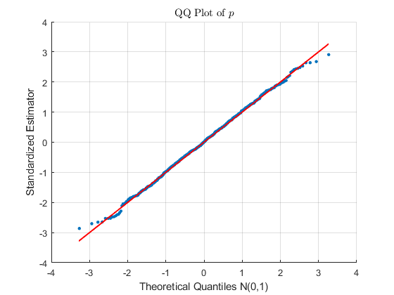
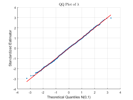
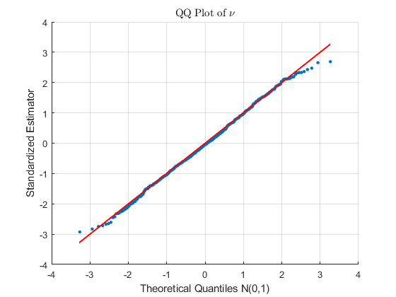
The collection of estimates over the 1,0001{,}000 runs yields an empirical distribution for each parameter. To assess the distributional behavior of the estimators, Q–Q plots of the standardized estimation errors are constructed, where each estimator is centered at its true value and scaled by its empirical standard deviation across runs. The resulting standardized samples are compared against the standard normal distribution. Figure 2 confirms that the proposed estimators are asymptotically normal.
Refer to caption
(a) λ=0.5\lambda=0.5
Refer to caption
(b) ν=2\nu=2
Refer to caption
(c) p=0.3p=0.3
Figure 2. Normal Q–Q plots of the standardized estimators for λ\lambda, μ\mu, and pp, where each estimator is centered at its true value (shown below each plot) and scaled by its empirical standard deviation computed from 1,000 independent replications.

4. Extensions

In this section, we discuss two types of extensions: (i) one concerning alternative observation schemes, and (ii) one allowing for more than two age groups.

4.1. Different observation schemes

In this subsection, we consider two observation schemes: one in which only the adults are observed, and one in which only the juveniles are observed. Remarkably, in the ‘Poisson setting’ (P), observing the juvenile time series (Xn)n≥0(X_{n})_{n\geq 0} allows us to identify all three model parameters, whereas observing the adult time series (Yn)n≥0(Y_{n})_{n\geq 0} leads to identifiability issues that prevent full parameter estimation.

4.1.1. Observing the adults

We first consider the situation in which the observed process is {Yn}n≥0\{Y_{n}\}_{n\geq 0}. We have that 𝔼​[Yn+1​Yn]=(𝔼​[Yn])2\mathbb{E}[Y_{n+1}Y_{n}]=(\mathbb{E}[Y_{n}])^{2}, as a consequence of the easily verifiable relation

𝔼​[Yn+1​Yn]=𝔼​[𝔼​[Bin​(Xn,p)​Yn|Xn]]=p​𝔼​[Xn​Yn]\mathbb{E}[Y_{n+1}Y_{n}]=\mathbb{E}\left[\mathbb{E}\big[{\rm Bin}(X_{n},p)Y_{n}\,|\,X_{n}\right]\big]=p\,\mathbb{E}[X_{n}Y_{n}]

and (2.20). As a consequence, we cannot base our estimator on (𝔼​[Yn],𝔼​[Yn2],𝔼​[Yn+1​Yn])(\mathbb{E}[Y_{n}],\mathbb{E}[Y_{n}^{2}],\mathbb{E}[Y_{n+1}Y_{n}]), since 𝔼​[Yn]\mathbb{E}[Y_{n}] and 𝔼​[Yn+1​Yn]\mathbb{E}[Y_{n+1}Y_{n}] provide essentially the same information. The following lemma shows that, in fact, the same identifiability issue arises if one replaces 𝔼​[Yn+1​Yn]\mathbb{E}[Y_{n+1}Y_{n}] by 𝔼​[Yn+k​Yn]\mathbb{E}[Y_{n+k}Y_{n}] for any k≥1k\geq 1. Define γ:=p​λ\gamma:=p\lambda and recall that ϱ=p​ν\varrho=p\nu.

Lemma 4.1.

Assume that (P) and (S) hold. Then the first and second moments of the observed adult population, namely 𝔼​[Yn]\mathbb{E}[Y_{n}] and 𝔼​[Yn2]\mathbb{E}[Y_{n}^{2}], as well as the cross-moments 𝔼​[Yn+k​Yn]\mathbb{E}[Y_{n+k}Y_{n}] for any k≥1k\geq 1, are functions of the parameters γ\gamma and ϱ\varrho only.

Proof.

By (2.20)–(2.22), we obtain that 𝔼​[Yn]\mathbb{E}[Y_{n}] and 𝔼​[Yn2]\mathbb{E}[Y_{n}^{2}] are functions of γ\gamma and ϱ\varrho:

𝔼​[Yn]=γ1−ϱ,𝔼​[Yn2]=γ1−ϱ+γ21−ϱ2+γ​ϱ​(ϱ+2​γ)(1−ϱ)​(1−ϱ2).\mathbb{E}[Y_{n}]=\dfrac{\gamma}{1-\varrho},\qquad\mathbb{E}[Y_{n}^{2}]=\dfrac{\gamma}{1-\varrho}+\dfrac{\gamma^{2}}{1-\varrho^{2}}+\dfrac{\gamma\varrho(\varrho+2\gamma)}{(1-\varrho)(1-\varrho^{2})}.

It remains to show that 𝔼​[Zn+k​Zn]\mathbb{E}[Z_{n+k}Z_{n}] depends solely on γ\gamma and ϱ\varrho. We do this by by induction over k≥1k\geq 1. For k=1k=1, we already saw that 𝔼​[Yn+1​Yn]=(𝔼​[Yn])2\mathbb{E}[Y_{n+1}Y_{n}]=(\mathbb{E}[Y_{n}])^{2}. Assume now that the claim holds for k≥1k\geq 1 and we prove it for k+1k+1. We find

𝔼​[Yn+k+1​Yn]\displaystyle\mathbb{E}[Y_{n+k+1}Y_{n}] =𝔼​[𝔼​[Bin​(Xn+k,p)​Yn|Xn+k]]=p​𝔼​[Xn+k​Yn]\displaystyle=\mathbb{E}\!\left[\mathbb{E}\!\left[{\rm Bin}(X_{n+k},p)\,Y_{n}\,\big|\,X_{n+k}\right]\right]=p\,\mathbb{E}[X_{n+k}Y_{n}]
=p​𝔼​[𝔼​[(In+k−1+∑i=1Yn+k−1Gn+k−1,i)​Yn|Yn+k−1]]=γ​𝔼​[Yn]+ϱ​𝔼​[Yn+k−1​Yn].\displaystyle=p\,\mathbb{E}\!\left[\mathbb{E}\!\left[\left(I_{n+k-1}+\sum_{i=1}^{Y_{n+k-1}}G_{n+k-1,i}\right)Y_{n}\,\Bigg|\,Y_{n+k-1}\right]\right]=\gamma\,\mathbb{E}[Y_{n}]+\varrho\,\mathbb{E}[Y_{n+k-1}Y_{n}].

If k≥2k\geq 2, then the claim follows by the induction hypothesis, otherwise it follows from the explicit expression of 𝔼​[Yn2]\mathbb{E}[Y_{n}^{2}]. This concludes the proof. ∎

A direct consequence of Lemma 4.1 is that, when using moments of the form 𝔼​[Yn]\mathbb{E}[Y_{n}], 𝔼​[Yn2]\mathbb{E}[Y_{n}^{2}], and 𝔼​[Yn+k​Yn]\mathbb{E}[Y_{n+k}Y_{n}], one can estimate only the combined quantities p​λp\lambda and p​νp\nu, but not the three parameters pp, λ\lambda, and ν\nu individually. Lemma 4.2 below further shows that considering higher-order moments 𝔼​[Ynk]\mathbb{E}[Y_{n}^{k}] alone does not resolve this issue, since the stationary distribution of YnY_{n} also depends solely on γ\gamma and ϱ\varrho. Define by ΨY​(⋅)\Psi_{Y}(\cdot) the probability generating function of YnY_{n} in stationarity. Let ϕϱ(j)​(⋅)\phi_{\varrho}^{(j)}(\cdot) denote the jj-th iterate of the map ϕϱ​(⋅)\phi_{\varrho}(\cdot) defined by x↦exp⁡(ϱ​(x−1))x\mapsto\exp(\varrho(x-1)).

Lemma 4.2.

Assume that (P) and (S) hold. Then,

ΨY​(s)=exp⁡(γ​∑j=0∞(ϕϱ(j)​(s)−1)).\Psi_{Y}(s)=\exp\Biggl(\gamma\sum_{j=0}^{\infty}\bigl(\phi_{\varrho}^{(j)}(s)-1\bigr)\Biggr).

In particular, the stationary distribution of YnY_{n} depends solely on γ\gamma and ϱ\varrho.

Proof.

By the Poisson thinning property, we know that if V∼Poisson​(λ)V\sim{\rm Poisson}(\lambda) and W|V∼Bin​(V,p)W\,|\,V\sim{\rm Bin}(V,p), then W∼Poisson​(p​λ)W\sim{\rm Poisson}(p\lambda). This implies that Yn+1∼Poisson​(γ+ϱ​Yn)Y_{n+1}\sim{\rm Poisson}(\gamma+\varrho Y_{n}). Let us denote by ΨYn​(⋅)\Psi_{Y_{n}}(\cdot) the probability generating function of YnY_{n}, i.e., ΨYn​(s)=𝔼​[sYn]\Psi_{Y_{n}}(s)=\mathbb{E}[s^{Y_{n}}], s∈[0,1]s\in[0,1]. Thus,

ΨYn+1​(s)=𝔼​[𝔼​[sYn+1|Yn]]=𝔼​[exp⁡(γ+ϱ​Yn)​(s−1)]=exp⁡(γ​(s−1))​ΨYn​(exp⁡(ϱ​(s−1))).\begin{array}[]{ll}\Psi_{Y_{n+1}}(s)&=\mathbb{E}\left[\mathbb{E}\left[s^{Y_{n+1}}|\,Y_{n}\right]\right]=\mathbb{E}\left[\exp(\gamma+\varrho Y_{n})(s-1)\right]\\ &=\exp(\gamma(s-1))\Psi_{Y_{n}}(\exp(\varrho(s-1))).\end{array}

In stationarity, we thus find

ΨY​(s)=eγ​(s−1)​ΨY​(eϱ​(s−1)).\Psi_{Y}(s)={\rm e}^{\gamma(s-1)}\Psi_{Y}\left({\rm e}^{\varrho(s-1)}\right). (4.1)

The goal is now to express ΨY​(s)\Psi_{Y}(s) in a form that depends only on γ\gamma and ϱ\varrho, thereby showing that the stationary distribution of the process {Yn}n≥0\{Y_{n}\}_{n\geq 0} also depends only on these quantities. To this end, consider the function ϕϱ​(s):=exp⁡(ϱ​(s−1))\phi_{\varrho}(s):=\exp\bigl(\varrho(s-1)\bigr), which maps the interval [0,1][0,1] into itself. It is straightforward to verify that s∗=1s^{*}=1 is a fixed point of the equation ϕϱ​(s)=s\phi_{\varrho}(s)=s, i.e., ϕϱ​(s∗)=s∗\phi_{\varrho}(s^{*})=s^{*}. By the Banach fixed point theorem, this fixed point is unique. Indeed, ϕϱ\phi_{\varrho} is a contraction, as ϕϱ′​(s)=ϱ​exp⁡(ϱ​(s−1))≤ϱ<1\phi_{\varrho}^{\prime}(s)=\varrho\exp(\varrho(s-1))\leq\varrho<1; here we have used that we imposed the stationary condition ϱ<1\varrho<1. Moreover, the theorem guarantees that the sequence defined recursively by sk+1=ϕϱ​(sk)s_{k+1}=\phi_{\varrho}(s_{k}), for k≥0k\geq 0 and any initial s0∈[0,1]s_{0}\in[0,1], converges to the fixed point:

limk→∞sk=limk→∞ϕϱ(k)​(s0)=1,\lim_{k\to\infty}s_{k}=\lim_{k\to\infty}\phi_{\varrho}^{(k)}(s_{0})=1,

where ϕϱ(k)\phi_{\varrho}^{(k)} denotes the kk-th iterate of ϕϱ\phi_{\varrho}. By iterating (4.1) kk times, we find

ΨY​(s)=exp⁡(γ​∑j=0k−1(ϕϱ(j)​(s)−1))​ΨY​(ϕϱ(k)​(s)).\Psi_{Y}(s)=\exp\left(\gamma\displaystyle\sum_{j=0}^{k-1}\left(\phi_{\varrho}^{(j)}(s)-1\right)\right)\Psi_{Y}\left(\phi_{\varrho}^{(k)}(s)\right).

Since ΨY​(s)\Psi_{Y}(s) is continuous at s=1s=1 and ΨY​(1)=1\Psi_{Y}(1)=1, we conclude

ΨY​(s)=limk→∞exp⁡(γ​∑j=0k−1(ϕϱ(j)​(s)−1))​ΨY​(ϕϱ(k)​(s))=exp⁡(γ​∑j=0∞(ϕϱ(j)​(s)−1)).\begin{array}[]{ll}\Psi_{Y}(s)&=\displaystyle\lim_{k\to\infty}\exp\left(\gamma\displaystyle\sum_{j=0}^{k-1}\left(\phi_{\varrho}^{(j)}(s)-1\right)\right)\Psi_{Y}\left(\phi_{\varrho}^{(k)}(s)\right)=\exp\left(\gamma\displaystyle\sum_{j=0}^{\infty}\left(\phi_{\varrho}^{(j)}(s)-1\right)\right).\end{array}

Observing that the function ϕϱ​(⋅)\phi_{\varrho}(\cdot) depends only on ϱ\varrho, this concludes the proof. ∎

4.1.2. Observing the juveniles

We proceed by considering the case that we observe (Xn)n≥0(X_{n})_{n\geq 0}. Similar to what we found for the case of observing (Yn)n≥0(Y_{n})_{n\geq 0}, we find that

𝔼​[Xn+1​Xn]=λ​𝔼​[Xn]+ν​𝔼​[Xn​Yn]=λ21−p​ν+p​ν​λ2(1−p​ν)2=λ2(1−p​ν)2=(𝔼​[Xn])2,\mathbb{E}[X_{n+1}X_{n}]=\lambda\mathbb{E}[X_{n}]+\nu\mathbb{E}[X_{n}Y_{n}]=\frac{\lambda^{2}}{1-p\nu}+\frac{p\nu\lambda^{2}}{(1-p\nu)^{2}}=\frac{\lambda^{2}}{(1-p\nu)^{2}}=(\mathbb{E}[X_{n}])^{2},

so that the moment equations based on 𝔼​[Xn]\mathbb{E}[X_{n}] and 𝔼​[Xn+1​Xn]\mathbb{E}[X_{n+1}X_{n}] effectively provide the same information. Unlike in the case of observing (Yn)n≥0(Y_{n})_{n\geq 0}, this complication can be remedied by working with the moments (𝔼​[Xn],𝔼​[Xn2],𝔼​[Xn+2​Xn])(\mathbb{E}[X_{n}],\mathbb{E}[X_{n}^{2}],\mathbb{E}[X_{n+2}X_{n}]), where we use the (readily verified) relation

𝔼​[Xn+2​Xn]=λ​𝔼​[Xn]+p​ν+𝔼​[Xn2].\mathbb{E}[X_{n+2}X_{n}]=\lambda\mathbb{E}[X_{n}]+p\nu+\mathbb{E}[X_{n}^{2}].

In particular, recalling the relations (2.20)–(2.22), it follows that 𝔼​[Xn+2​Xn]\mathbb{E}[X_{n+2}X_{n}] cannot be expressed in terms of γ\gamma and ϱ\varrho only. The next lemma shows that, more generally, the stationary distribution of XnX_{n} does not depend only on γ\gamma and ϱ\varrho. Define by ΨX​(⋅)\Psi_{X}(\cdot) the probability generating function of XnX_{n} in stationarity. Recall that ϕϱ(j)​(⋅)\phi_{\varrho}^{(j)}(\cdot) denotes the jj-th iterate of the map ϕϱ​(⋅)\phi_{\varrho}(\cdot) defined by x↦exp⁡(ϱ​(x−1))x\mapsto\exp(\varrho(x-1)).

Lemma 4.3.

Assume that (P) and (S) hold. Then,

ΨX​(s)=exp⁡(λ​(s−1))​exp⁡(γ​∑j=0∞(ϕϱ(j)​(exp⁡(ν​(s−1)))−1)).\Psi_{X}(s)=\exp\left(\lambda(s-1)\right)\exp\left(\gamma\displaystyle\sum_{j=0}^{\infty}\left(\phi_{\varrho}^{(j)}\left(\exp\left(\nu(s-1)\right)\right)-1\right)\right).

In particular, the stationary distribution of YnY_{n} does not depend solely on γ\gamma and ϱ\varrho.

Proof.

By noting that Xn+1∼Poisson​(λ+ν​Yn)X_{n+1}\sim{\rm Poisson}(\lambda+\nu Y_{n}), the probability generating function ΨXn+1​(⋅)\Psi_{X_{n+1}}(\cdot) of Xn+1X_{n+1} can be written as

ΨXn+1​(s)=𝔼​[𝔼​[sXn+1|Yn]]=exp⁡(λ​(s−1))​𝔼​[exp⁡(ν​(s−1)​Yn)]=exp⁡(λ​(s−1))​ΨYn​(exp⁡(ν​(s−1))).\begin{array}[]{ll}\Psi_{X_{n+1}}(s)&=\mathbb{E}\left[\mathbb{E}\left[s^{X_{n+1}}\,|\,Y_{n}\right]\right]=\exp(\lambda(s-1))\mathbb{E}[\exp(\nu(s-1)Y_{n})]\\ &=\exp(\lambda(s-1))\Psi_{Y_{n}}(\exp(\nu(s-1))).\end{array}

As a consequence, in stationarity,

ΨX​(s)=exp⁡(λ​(s−1))​ΨY​(exp⁡(ν​(s−1)))=exp⁡(λ​(s−1))​exp⁡(γ​∑j=0∞(ϕϱ(j)​(exp⁡(ν​(s−1)))−1)).\begin{array}[]{ll}\Psi_{X}(s)&=\exp(\lambda(s-1))\Psi_{Y}(\exp(\nu(s-1)))\\ &=\exp\left(\lambda(s-1)\right)\exp\left(\gamma\displaystyle\sum_{j=0}^{\infty}\left(\phi_{\varrho}^{(j)}\left(\exp\left(\nu(s-1)\right)\right)-1\right)\right).\end{array}

Since the prefactor depends explicitly on λ\lambda, and the argument of the iterates ϕϱ(j)\phi_{\varrho}^{(j)}, with j≥0j\geq 0, depends explicitly on ν\nu, the stationary distribution of XnX_{n} does not depend only on γ\gamma and ϱ\varrho. ∎

Remark 4.4.

The asymmetry in the limiting distributions of YnY_{n} and XnX_{n}, as observed above, stems from the fundamentally different roles played by thinning and Poisson summation in their recursive definitions. At each step, YnY_{n} is thinned by pp, and therefore the thinning factor pp appears linearly in the stationary probability generating function. This makes the stationary distribution depend only on γ\gamma and ϱ\varrho. On the other hand, XnX_{n} is the sum of Yn−1+1Y_{n-1}+1 Poisson random variables, so the parameters λ\lambda and ν\nu enter directly. This means that the stationary distribution of XnX_{n} cannot be expressed in terms of γ\gamma and ϱ\varrho alone. ♠\spadesuit

4.2. More age groups

In the model considered so far, we distinguished between juveniles and a single adult group. The adult population was assumed to be homogeneous with respect to fertility, and immigration was allowed only into the juvenile class. In this section, we show that this framework can be generalized in several natural and important directions.

First, instead of working with only two age classes, we may consider KK age groups for any K∈ℕK\in\mathbb{N}, and allow immigration to occur in any of these groups. Second, each age group may contribute to the production of juveniles through its own offspring distribution.

The purpose of this section is to demonstrate that the analysis developed in Sections 2–3 extends to this considerably more general setting. We emphasize, however, that this extension comes at the cost of substantially more involved computations, which we have chosen not to present in detail, as they offer limited additional insight. For example, in the discussion of asymptotic normality in Section 3, the associated covariance matrix contains 12​(K+1)​(K+2)\tfrac{1}{2}(K+1)(K+2) distinct elements, each of which must be computed explicitly. It is worth noting, however, that from a conceptual point of view, these calculations closely mirror those developed in Section 3.

In this general setup, the branching process under study has KK types: the juveniles that are recorded via the process {Xn}n≥0{\smash{\{}X_{n}\}_{n\geq 0}}, and the kk-group of adults by {Yn(k)}n≥0{\smash{\{}Y^{(k)}_{n}\}_{n\geq 0}}, for k=1,…,Kk=1,\ldots,K. Then the dynamics are governed by the following (K+1)(K+1)-dimensional stochastic recursion:

Xn+1\displaystyle X_{n+1} =In(0)+∑k=1K∑i=1Yn(k)Gn,i(k),\displaystyle=I_{n}^{(0)}+\sum_{k=1}^{K}\sum_{i=1}^{Y_{n}^{(k)}}G^{(k)}_{n,i}, Yn+1(1)∼In(1)+Bin​(Xn,p1),Yn+1(2)∼In(2)+Bin​(Yn(1),p2),⋮Yn+1(K)∼In(K)+Bin​(Yn(K−1),pK),\displaystyle\hskip 36.98866pt\begin{aligned} Y_{n+1}^{(1)}&\sim I_{n}^{(1)}+\mathrm{Bin}(X_{n},p_{1}),\\ Y_{n+1}^{(2)}&\sim I_{n}^{(2)}+\mathrm{Bin}(Y_{n}^{(1)},p_{2}),\\ &\ \vdots\\ Y_{n+1}^{(K)}&\sim I_{n}^{(K)}+\mathrm{Bin}(Y_{n}^{(K-1)},p_{K}),\end{aligned}

where the random sequences involved in the model are such that

In(k)\displaystyle I_{n}^{(k)} ∼i.i.d.  as ​I(k)∈ℕ0,\displaystyle\sim\text{i.i.d.\ \,as }I^{(k)}\in{\mathbb{N}}_{0}, n≥0,\displaystyle n\geq 0,\quad k=0,…,K,\displaystyle k=0,\dots,K,
Gn,i(k)\displaystyle G_{n,i}^{(k)} ∼i.i.d.  as ​G(k)∈ℕ0,\displaystyle\sim\text{i.i.d.\ \,as }G^{(k)}\in{\mathbb{N}}_{0}, n,i≥1,\displaystyle n,i\geq 1,\quad k=1,…,K,\displaystyle k=1,\dots,K,

with all sequences {In(k)}n≥0\{I_{n}^{(k)}\}_{n\geq 0} and {Gn,i(k)}n≥0\{G_{n,i}^{(k)}\}_{n\geq 0} being mutually independent.

We now explain how to compute the stationary mean of the process, using a calculation that simultaneously reveals the model’s stability condition. It is readily checked that in stationarity one has, with 𝑰≡(I(0),…,I(K))⊤{\boldsymbol{I}}\equiv(I^{(0)},\ldots,I^{(K)})^{\top} and 𝑾n≡(Xn,Yn(1),…,Yn(K)){\boldsymbol{W}}_{n}\equiv(X_{n},Y_{n}^{(1)},\ldots,Y_{n}^{(K)}),

𝔼​[𝑾n+1]=𝔼​[𝑰]+D(K)​𝔼​[𝑾n],\mathbb{E}[{\boldsymbol{W}}_{n+1}]=\mathbb{E}[{\boldsymbol{I}}]+D^{(K)}\,\mathbb{E}[{\boldsymbol{W}}_{n}],

where

D(K):=(0𝔼​[G(1)]𝔼​[G(2)]⋯𝔼​[G(K−1)]𝔼​[G(K)]p100⋯000p20⋯00⋮⋮⋮⋱⋮⋮000⋯pK0).D^{(K)}:=\left(\begin{array}[]{cccccc}0&\mathbb{E}[G^{(1)}]&\mathbb{E}[G^{(2)}]&\cdots&\mathbb{E}[G^{(K-1)}]&\mathbb{E}[G^{(K)}]\\ p_{1}&0&0&\cdots&0&0\\ 0&p_{2}&0&\cdots&0&0\\ \vdots&\vdots&\vdots&\ddots&\vdots&\vdots\\ 0&0&0&\cdots&p_{K}&0\end{array}\right).

It follows that the stationary mean is, provided that spectral radius of D(K)D^{(K)} is strictly smaller than 11,

𝔼​[𝑾n]=(I−D(K))−1​𝔼​[𝑰].\mathbb{E}[{\boldsymbol{W}}_{n}]=\left(I-D^{(K)}\right)^{-1}\mathbb{E}[{\boldsymbol{I}}].

Appendix B presents a worked example for K=2K=2, including detailed computations of the underlying moment expressions.

5. Discussion and concluding remarks

In this paper, we developed a method-of-moments approach for estimating the parameters of an age-dependent branching process from observations of the total population size alone. In the ergodic regime, we established the asymptotic normality of the resulting estimator and illustrated that the approach extends naturally to several more general settings, including models with multiple age groups. We hope that these results provide a useful basis for statistical inference in age-structured branching models and may serve as a starting point for further developments in more general observation schemes or model classes.

Several directions for future research appear promising. A natural extension is the statistical analysis of sex-structured age-dependent branching processes, where the interaction between age and sex raises new modeling and identifiability challenges. Another interesting direction is to study estimation under more general observation schemes, such as irregular or noisy observations, or in the presence of missing data. It would also be worthwhile to investigate inference beyond the ergodic regime, where the long-term behavior of the process is fundamentally different, and to develop likelihood-based or Bayesian estimation procedures that can be compared, both theoretically and numerically, with the method-of-moments approach considered here.

Appendix A Explicit expressions for stationary moments

We now illustrate how to compute 𝕊​[𝑽0(1)]\smash{{\mathbb{S}}[{\boldsymbol{V}}_{0}^{(1)}]}, 𝕊​[𝑽0(2)]\smash{{\mathbb{S}}[{\boldsymbol{V}}_{0}^{(2)}]}, 𝕊​[𝑽0(12)]\smash{{\mathbb{S}}[{\boldsymbol{V}}_{0}^{(12)}]}, 𝕊​[𝑽0(1),𝑽0(2)]\smash{{\mathbb{S}}[{\boldsymbol{V}}_{0}^{(1)},{\boldsymbol{V}}_{0}^{(2)}]}, 𝕊​[𝑽0(1),𝑽0(12)]\smash{{\mathbb{S}}[{\boldsymbol{V}}_{0}^{(1)},{\boldsymbol{V}}_{0}^{(12)}]}, 𝕊​[𝑽0(2),𝑽0(12)]\smash{{\mathbb{S}}[{\boldsymbol{V}}_{0}^{(2)},{\boldsymbol{V}}_{0}^{(12)}]}. To derive these quantities, we first define the following auxiliary variables:

𝑵n(1):=(Xn,Yn)⊤\displaystyle{\boldsymbol{N}}_{n}^{(1)}:=(X_{n},Y_{n})^{\top}
𝑵n(2):=(Xn2,Xn​Yn,Yn2)⊤\displaystyle{\boldsymbol{N}}_{n}^{(2)}:=(X_{n}^{2},X_{n}Y_{n},Y_{n}^{2})^{\top}
𝑵n(3):=(Xn3,Xn2​Yn,Xn​Yn2,Yn3)⊤\displaystyle{\boldsymbol{N}}_{n}^{(3)}:=(X_{n}^{3},X_{n}^{2}Y_{n},X_{n}Y_{n}^{2},Y_{n}^{3})^{\top}
𝑵n(4):=(Xn4,Xn3​Yn,Xn2​Yn2,Xn​Yn3,Yn4)⊤.\displaystyle{\boldsymbol{N}}_{n}^{(4)}:=(X_{n}^{4},X_{n}^{3}Y_{n},X_{n}^{2}Y_{n}^{2},X_{n}Y_{n}^{3},Y_{n}^{4})^{\top}\,.

Equation (2.6) provides the expression for 𝔼​𝑵n(1)\mathbb{E}{\boldsymbol{N}}_{n}^{(1)}. We now show how 𝔼​𝑵n(2)\mathbb{E}{\boldsymbol{N}}_{n}^{(2)} can be computed based on 𝔼​𝑵n(1)\mathbb{E}{\boldsymbol{N}}_{n}^{(1)}.

(I) We observe that 𝑵n(2)=𝑽n(2){\boldsymbol{N}}_{n}^{(2)}={\boldsymbol{V}}^{(2)}_{n}. As established earlier in part (B), we have

𝔼​[𝑽n(2)|Xn−1=k,Yn−1=ℓ]\displaystyle\mathbb{E}\left[{\boldsymbol{V}}^{(2)}_{n}\,\Big|\,X_{n-1}=k,Y_{n-1}=\ell\right] =(𝔼​[I2]+𝔽​[G,I]​ℓ+(𝔼​[G])2​ℓ2p​𝔼​[I]​k+p​𝔼​[G]​k​ℓp​(1−p)​k+p2​k2)\displaystyle=\left(\begin{array}[]{c}\mathbb{E}[I^{2}]+{\mathbb{F}}[G,I]\,\ell+(\mathbb{E}[G])^{2}\ell^{2}\\ p\,\mathbb{E}[I]\,k+p\,\mathbb{E}[G]\,k\ell\\ p(1-p)\,k+p^{2}\,k^{2}\end{array}\right)
=𝒃2+C2,1​(kℓ)+C2,2​(k2k​ℓℓ2).\displaystyle={\boldsymbol{b}}_{2}+C_{2,1}\left(\begin{array}[]{c}k\\ \ell\end{array}\right)+C_{2,2}\left(\begin{array}[]{c}k^{2}\\ k\ell\\ \ell^{2}\end{array}\right).

where

𝒃2=(𝔼​[I2]00)C2,1=(0𝔽​[G,I]p​𝔼​[I]0p​(1−p)0)C2,2=(00(𝔼​[G])20p​𝔼​[G]0p200).{\boldsymbol{b}}_{2}=\left(\begin{array}[]{c}\mathbb{E}[I^{2}]\\ 0\\ 0\end{array}\right)\qquad C_{2,1}=\left(\begin{array}[]{cc}0&{\mathbb{F}}[G,I]\\ p\,\mathbb{E}[I]&0\\ p(1-p)&0\end{array}\right)\qquad C_{2,2}=\left(\begin{array}[]{ccc}0&0&({\mathbb{E}}[G])^{2}\\ 0&p\,\mathbb{E}[G]&0\\ p^{2}&0&0\end{array}\right)\,.

Thus, as n→∞n\rightarrow\infty, in stationarity,

𝔼​𝑵n(2)=𝒃2+C2,1​𝔼​𝑵n(1)+C2,2​𝔼​𝑵n(2)\mathbb{E}{\boldsymbol{N}}_{n}^{(2)}={\boldsymbol{b}}_{2}+C_{2,1}\mathbb{E}{\boldsymbol{N}}_{n}^{(1)}+C_{2,2}\mathbb{E}{\boldsymbol{N}}_{n}^{(2)}

Rearranging terms yields

𝔼​𝑵n(2)=(I−C2,2)−1​(𝒃2+C2,1​𝔼​𝑵n(1)).\mathbb{E}{\boldsymbol{N}}_{n}^{(2)}=(I-C_{2,2})^{-1}\,({\boldsymbol{b}}_{2}+C_{2,1}\mathbb{E}{\boldsymbol{N}}_{n}^{(1)})\,.

(II) Similarly, we can write

𝔼​[𝑵n(3)|Xn−1=k,Yn−1=ℓ]=𝒃3+C3,1​(kℓ)+C3,2​(kℓ)+C2,2​(k2k​ℓℓ2)+C3,3​(k3k2​ℓk​ℓ2ℓ3),\mathbb{E}\left[{\boldsymbol{N}}^{(3)}_{n}\,\Big|\,X_{n-1}=k,Y_{n-1}=\ell\right]={\boldsymbol{b}}_{3}+C_{3,1}\left(\begin{array}[]{c}k\\ \ell\end{array}\right)+C_{3,2}\left(\begin{array}[]{c}k\\ \ell\end{array}\right)+C_{2,2}\left(\begin{array}[]{c}k^{2}\\ k\ell\\ \ell^{2}\end{array}\right)+C_{3,3}\left(\begin{array}[]{c}k^{3}\\ k^{2}\ell\\ k\ell^{2}\\ \ell^{3}\end{array}\right)\,,

where

C3,1=(03​𝔼​[I2]​𝔼​[G]+3​𝔼​[I]​𝕍​ar​[G]+𝔼​[G3]−3​𝔼​[G]​𝔼​[G2]+2​(𝔼​[G])3p​𝔼​[I2]0p​(1−p)​𝔼​[I]p​(1−p)​𝔼​[G]p​(1−p)​(1−2​p)0),\displaystyle C_{3,1}=\left(\begin{array}[]{cc}0&3\,\mathbb{E}[I^{2}]\,\mathbb{E}[G]+3\,\mathbb{E}[I]\,{\mathbb{V}}{\rm ar}[G]+\mathbb{E}[G^{3}]-3\,\mathbb{E}[G]\,\mathbb{E}[G^{2}]+2(\mathbb{E}[G])^{3}\\ p\,\mathbb{E}[I^{2}]&0\\ p(1-p)\,\mathbb{E}[I]&p(1-p)\,\mathbb{E}[G]\\ p(1-p)(1-2p)&0\end{array}\right),
C3,2=(003​𝔼​[I]​(𝔼​[G])2+3​𝔼​[G]​𝕍​ar​[G]0p​(2​𝔼​[I]​𝔼​[G]+𝔼​[G2])p​(𝔼​[G])2p2​𝔼​[I]003​p2​(1−p)00),\displaystyle C_{3,2}=\left(\begin{array}[]{ccc}0&0&3\,\mathbb{E}[I](\mathbb{E}[G])^{2}+3\,\mathbb{E}[G]\,{\mathbb{V}}{\rm ar}[G]\\ 0&p\bigl(2\,\mathbb{E}[I]\,\mathbb{E}[G]+\mathbb{E}[G^{2}]\bigr)&p(\mathbb{E}[G])^{2}\\ p^{2}\,\mathbb{E}[I]&0&0\\ 3p^{2}(1-p)&0&0\end{array}\right),
C3,3=(000(𝔼​[G])300000000p3000),𝒃3=(𝔼​[I3]000).\displaystyle C_{3,3}=\left(\begin{array}[]{cccc}0&0&0&(\mathbb{E}[G])^{3}\\ 0&0&0&0\\ 0&0&0&0\\ p^{3}&0&0&0\end{array}\right),\qquad\qquad{\boldsymbol{b}}_{3}=\left(\begin{array}[]{c}\mathbb{E}[I^{3}]\\ 0\\ 0\\ 0\end{array}\right)\,.

Then, in stationarity, we have

𝔼​𝑵n(3)=(I−C3,3)−1​(𝒃3+C3,1​𝔼​𝑵n(1)+C3,2​𝔼​𝑵n(2)).\mathbb{E}{\boldsymbol{N}}_{n}^{(3)}=(I-C_{3,3})^{-1}\,({\boldsymbol{b}}_{3}+C_{3,1}\mathbb{E}{\boldsymbol{N}}_{n}^{(1)}+C_{3,2}\mathbb{E}{\boldsymbol{N}}_{n}^{(2)})\,.

Appendix B Branching process with three age groups

In this appendix we determine stationary moments for a branching process with three age groups, with arguments similar to those that have been used for two age groups. Consider the branching process

Xn+1=In(0)+∑k=12∑i=1Yn(k)Gk,i,Yn+1(1)∣Xn∼In(1)+Bin​(Xn,p1),Yn+1(2)∣Yn(1)∼In(2)+Bin​(Yn(1),p2).X_{n+1}=I_{n}^{(0)}+\sum_{k=1}^{2}\sum_{i=1}^{Y_{n}^{(k)}}G_{k,i},\quad Y_{n+1}^{(1)}\mid X_{n}\sim I_{n}^{(1)}+\mathrm{Bin}(X_{n},p_{1}),\quad Y_{n+1}^{(2)}\mid Y_{n}^{(1)}\sim I_{n}^{(2)}+\mathrm{Bin}(Y_{n}^{(1)},p_{2}).

where In(k)∼Poisson​(λk)I_{n}^{(k)}\sim\mathrm{Poisson}(\lambda_{k}) for k=0,1,2,k=0,1,2, and Gk,i∼Poisson​(ν),G_{k,i}\sim\mathrm{Poisson}(\nu), and all random variables are mutually independent. Write g1:=𝔼​[G]=νg_{1}:=\mathbb{E}[G]=\nu and g2:=𝔼​[G2]=ν+ν2,g_{2}:=\mathbb{E}[G^{2}]=\nu+\nu^{2}, and define Zn:=Xn+Yn(1)+Yn(2).Z_{n}:=X_{n}+Y_{n}^{(1)}+Y_{n}^{(2)}. Taking expectations and solving the stationary balance equations yields

μ:=𝔼​[Xn]=λ0+g1​[λ1​(1+p2)+λ2]1−g1​p1​(1+p2),\mu:=\mathbb{E}[X_{n}]=\frac{\lambda_{0}+g_{1}[\lambda_{1}(1+p_{2})+\lambda_{2}]}{1-g_{1}p_{1}(1+p_{2})},

together with α:=𝔼​[Yn(1)]=λ1+p1​μ\alpha:=\mathbb{E}[Y_{n}^{(1)}]=\lambda_{1}+p_{1}\mu and β:=𝔼​[Yn(2)]=λ2+p2​α,\beta:=\mathbb{E}[Y_{n}^{(2)}]=\lambda_{2}+p_{2}\alpha, so that

𝔼​[Zn]=μ+α+β=[λ0+g1​(λ1​(1+p2)+λ2)]​(1+p1+p1​p2)1−g1​p1​(1+p2)+λ1​(1+p2)+λ2.\mathbb{E}[Z_{n}]=\mu+\alpha+\beta=\frac{\bigl[\lambda_{0}+g_{1}(\lambda_{1}(1+p_{2})+\lambda_{2})\bigr](1+p_{1}+p_{1}p_{2})}{1-g_{1}p_{1}(1+p_{2})}+\lambda_{1}(1+p_{2})+\lambda_{2}.

Next, let

𝒗:=(𝔼​[Xn2],𝔼​[(Yn(1))2],𝔼​[(Yn(2))2],𝔼​[Xn​Yn(1)],𝔼​[Xn​Yn(2)],𝔼​[Yn(1)​Yn(2)])⊤.\boldsymbol{v}:=\bigl(\mathbb{E}[X_{n}^{2}],\ \mathbb{E}[(Y_{n}^{(1)})^{2}],\ \mathbb{E}[(Y_{n}^{(2)})^{2}],\ \mathbb{E}[X_{n}Y_{n}^{(1)}],\ \mathbb{E}[X_{n}Y_{n}^{(2)}],\ \mathbb{E}[Y_{n}^{(1)}Y_{n}^{(2)}]\bigr)^{\top}.

Standard conditional moment calculations show that 𝒗=C+A​𝒗,\boldsymbol{v}={C}+{A}\boldsymbol{v}, where

C=(λ0+λ02+(2​λ0​g1+g2−g12)​(α+β)λ1+λ12+2​p1​λ1​μ+p1​(1−p1)​μλ2+λ22+2​p2​λ2​α+p2​(1−p2)​αλ0​λ1+λ0​p1​μ+g1​λ1​(α+β)λ0​λ2+λ0​p2​α+g1​λ2​(α+β)λ1​λ2+p2​λ1​α+p1​λ2​μ),A=(0g12g12002​g12p12000000p220000000g1​p1g1​p100g1​p2000g1​p2000p1​p200),{C}=\begin{pmatrix}\lambda_{0}+\lambda_{0}^{2}+(2\lambda_{0}g_{1}+g_{2}-g_{1}^{2})(\alpha+\beta)\\[5.0pt] \lambda_{1}+\lambda_{1}^{2}+2p_{1}\lambda_{1}\mu+p_{1}(1-p_{1})\mu\\[5.0pt] \lambda_{2}+\lambda_{2}^{2}+2p_{2}\lambda_{2}\alpha+p_{2}(1-p_{2})\alpha\\[5.0pt] \lambda_{0}\lambda_{1}+\lambda_{0}p_{1}\mu+g_{1}\lambda_{1}(\alpha+\beta)\\[5.0pt] \lambda_{0}\lambda_{2}+\lambda_{0}p_{2}\alpha+g_{1}\lambda_{2}(\alpha+\beta)\\[5.0pt] \lambda_{1}\lambda_{2}+p_{2}\lambda_{1}\alpha+p_{1}\lambda_{2}\mu\end{pmatrix},\qquad{A}=\begin{pmatrix}0&g_{1}^{2}&g_{1}^{2}&0&0&2g_{1}^{2}\\ p_{1}^{2}&0&0&0&0&0\\ 0&p_{2}^{2}&0&0&0&0\\ 0&0&0&g_{1}p_{1}&g_{1}p_{1}&0\\ 0&g_{1}p_{2}&0&0&0&g_{1}p_{2}\\ 0&0&0&p_{1}p_{2}&0&0\end{pmatrix},

so that 𝒗=(I−A)−1​C.\boldsymbol{v}=({I}-{A})^{-1}{C}.

The second moment and lag-one cross moment of ZnZ_{n} are linear functions of 𝒗\boldsymbol{v}. Indeed,

𝔼​[Zn2]=v1+v2+v3+2​v4+2​v5+2​v6.\mathbb{E}[Z_{n}^{2}]=v_{1}+v_{2}+v_{3}+2v_{4}+2v_{5}+2v_{6}.

Moreover, using conditional expectations,

𝔼​[Xn​Xn+1]\displaystyle\mathbb{E}[X_{n}X_{n+1}] =λ0​μ+g1​(v4+v5),\displaystyle=\lambda_{0}\mu+g_{1}(v_{4}+v_{5}), 𝔼​[Xn​Yn+1(1)]\displaystyle\mathbb{E}[X_{n}Y_{n+1}^{(1)}] =λ1​μ+p1​v1,\displaystyle=\lambda_{1}\mu+p_{1}v_{1},
𝔼​[Xn​Yn+1(2)]\displaystyle\mathbb{E}[X_{n}Y_{n+1}^{(2)}] =λ2​μ+p2​v4,\displaystyle=\lambda_{2}\mu+p_{2}v_{4}, 𝔼​[Yn(1)​Xn+1]\displaystyle\mathbb{E}[Y_{n}^{(1)}X_{n+1}] =λ0​α+g1​(v2+v6),\displaystyle=\lambda_{0}\alpha+g_{1}(v_{2}+v_{6}),
𝔼​[Yn(1)​Yn+1(1)]\displaystyle\mathbb{E}[Y_{n}^{(1)}Y_{n+1}^{(1)}] =λ1​α+p1​v4,\displaystyle=\lambda_{1}\alpha+p_{1}v_{4}, 𝔼​[Yn(1)​Yn+1(2)]\displaystyle\mathbb{E}[Y_{n}^{(1)}Y_{n+1}^{(2)}] =λ2​α+p2​v2,\displaystyle=\lambda_{2}\alpha+p_{2}v_{2},
𝔼​[Yn(2)​Xn+1]\displaystyle\mathbb{E}[Y_{n}^{(2)}X_{n+1}] =λ0​β+g1​(v3+v6),\displaystyle=\lambda_{0}\beta+g_{1}(v_{3}+v_{6}), 𝔼​[Yn(2)​Yn+1(1)]\displaystyle\mathbb{E}[Y_{n}^{(2)}Y_{n+1}^{(1)}] =λ1​β+p1​v5,\displaystyle=\lambda_{1}\beta+p_{1}v_{5},
𝔼​[Yn(2)​Yn+1(2)]\displaystyle\mathbb{E}[Y_{n}^{(2)}Y_{n+1}^{(2)}] =λ2​β+p2​v6.\displaystyle=\lambda_{2}\beta+p_{2}v_{6}.

Summing these terms gives

𝔼​[Zn​Zn+1]=(λ0+λ1+λ2)​(μ+α+β)+g1​(v2+v3+v4+v5+2​v6)+p1​(v1+v4+v5)+p2​(v2+v4+v6).\mathbb{E}[Z_{n}Z_{n+1}]=(\lambda_{0}+\lambda_{1}+\lambda_{2})(\mu+\alpha+\beta)+g_{1}(v_{2}+v_{3}+v_{4}+v_{5}+2v_{6})+p_{1}(v_{1}+v_{4}+v_{5})+p_{2}(v_{2}+v_{4}+v_{6}).

We evaluate the performance of the proposed estimation procedure through a simulation study. The true parameter values are set to

λ0=0.7,λ1=0.2,λ2=0.1,ν=0.8,p1=p2=p=0.4.\lambda_{0}=0.7,\quad\lambda_{1}=0.2,\quad\lambda_{2}=0.1,\quad\nu=0.8,\quad p_{1}=p_{2}=p=0.4.

We assume that λ1\lambda_{1} and λ2\lambda_{2} are known, and estimate the remaining parameters λ0\lambda_{0}, ν\nu, and pp. The simulation study consists of 1,0001{,}000 independent replications. In each replication, the system is observed over a time horizon N=105N=10^{5}, based on which the parameters λ0\lambda_{0}, ν\nu, and pp are estimated. Each replication yields one independent realization of the estimator for each parameter.

The Q–Q plots are then constructed using the 1,0001{,}000 resulting independent estimates for each parameter across replications. To assess the finite-sample distribution of the estimators, Figure 3 present normal Q–Q plots of the standardized estimators for λ0\lambda_{0}, ν\nu, and pp, respectively. In all three cases, the sample quantiles closely track the theoretical normal quantiles, indicating that the empirical distributions of the estimators are well approximated by Gaussian distributions. Of course, alternative specifications are also possible; in particular, we considered the case in which p1p_{1}, p2p_{2}, and ν\nu are unknown and found comparable estimation performance.
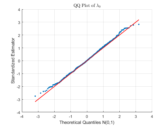
Refer to caption
(a) λ0\lambda_{0}
Refer to caption
(b) ν\nu
Refer to caption
(c) pp
Figure 3. Normal Q–Q plots of the standardized estimators for λ0\lambda_{0}, μ\mu, and pp. Each estimator is standardized by subtracting its true value and dividing by its empirical standard deviation obtained from 1,000 independent replications.

References

  • [1] Aït-Sahalia, Y., Cacho-Diaz, J., and Laeven, R. (2015). Modeling financial contagion using mutually exciting jump processes. Journal of Financial Economics, 117, pp. 585–606.
  • [2] Athreya, K. and Ney, P. (1972). Branching Processes. Springer, Berlin.
  • [3] Baldassarri, S. and Wang, J. (2025). Parameter estimation in interacting particle systems on dynamic random networks. Physical Review E, 112, 054301.
  • [4] Beaumont, M., Zhang, W., and Balding, D. (2002). Approximate Bayesian computation in population genetics. Genetics, 162, pp. 2025–2035.
  • [5] Cappé, O., Moulines, E., and Rydén, T. (2005). Inference in Hidden Markov Models. Springer, New York, NY.
  • [6] Cappé, O., Gordon, N., and Rydén, T. (2007). An overview of existing methods and recent advances in sequential Monte Carlo. Proceedings of the IEEE, 95(5), pp. 899–924.
  • [7] Casella, G. and Berger, R. (2002). Statistical Inference, 2nd ed. Duxbury Press, Belmont, CA.
  • [8] Caswell, H. (2001). Matrix Population Models: Construction, Analysis, and Interpretation, 2nd ed. Sinauer Associates, Sunderland, MA.
  • [9] Cauchemez, S. and Ferguson, N. (2008). Likelihood-based estimation of continuous-time epidemic models from time-series data: application to measles transmission in London. Journal of the Royal Society Interface, 5, pp. 885–897.
  • [10] Dempster, A., Laird, N., and Rubin, D. (1977). Maximum likelihood from incomplete data via the EM algorithm. Journal of the Royal Statistical Society, Series B, 39(1), pp. 1–22.
  • [11] Doucet, A., de Freitas, N., and Gordon, N. (eds.) (2001). Sequential Monte Carlo Methods in Practice. Springer, New York, NY.
  • [12] Duffie, D. and Glynn, P. (2004). Estimation of continuous-time Markov processes sampled at random time intervals. Econometrica, 72, pp. 1773–1808.
  • [13] Gupta, H., Mandjes, M., Ravner, L., and Wang, J. (2025). Uncovering the topology of an infinite-server queueing network from population data. arXiv:2506.07057, https://doi.org/10.48550/arXiv.2506.07057.
  • [14] Guttorp, P. (1991). Statistical Inference for Branching Processes. Wiley, Chichester, UK.
  • [15] Hazra, R.S., Mandjes, M., and Wang, J (2025). Parameter estimation in a dynamic Chung-Lu random graph. Physical Review E, 112, 014315.
  • [16] Hansen, M. and Pitts, S. (2006). Nonparametric inference from the M/G/1 workload. Bernoulli, 12, pp. 737–759.
  • [17] Ibragimov, I. (1962). Some limit theorems for stationary processes. Theory of Probability and Its Applications, 7(4), pp. 349–382.
  • [18] Kallenberg, O. (2002). Foundations of Modern Probability, 2nd ed. Springer, New York, NY.
  • [19] Lehmann, E. and Casella, G. (1998). Theory of Point Estimation, 2nd ed. Springer, New York, NY.
  • [20] Mandjes, M. and Wang, J. (2026). Estimation of on- and off-time distributions in a dynamic Erdős-Rényi random graph. Advances in Applied Probability, to appear. arXiv:2401.14531, https://arxiv.org/abs/2401.14531
  • [21] Peccati, G. and Taqqu, M. (2011). Wiener Chaos: Moments, Cumulants and Diagrams: A Survey with Computer Implementation. Springer, New York, NY.
  • [22] Ravner, L., Boxma, O., and Mandjes, M. (2019). Estimating the input of a Lévy-driven queue by Poisson sampling of the workload process. Bernoulli, 25, pp. 3734–3769.
  • [23] Sisson, S., Fan, Y., and Tanaka, M. (2018). Handbook of Approximate Bayesian Computation. CRC Press, Boca Raton, FL.
  • [24] van der Vaart, A. (1998). Asymptotic Statistics. Cambridge University Press, Cambridge.