A Transport Theory of Turbulent Coronal Heating in General GeometryPreprint: APS/123-QED

The expansion procedure yields equations describing how turbulence in any local patch depends on gradients of the slowly varying background. We thus introduce the following compact notation to capture the (inverse) scale length of a background $\mathcal{O}(\epsilon^{0})$ quantity $G$:

The perpendicular gradient operator $\nabla_{\perp}$ is defined by $\nabla_{\perp}G\equiv\nabla G-\hat{\bm{b}}\,\hat{\bm{b}}\cdot\!\nabla G$ (note that $\hat{\bm{b}}$ is the direction of the background field $\bm{B}=\langle\bm{B}^{(0)}\rangle$, and does not include contributions from perturbations). The ordering parameter is then the usual anisotropic RMHD ordering parameter, with $\epsilon\ll 1$ and

where $\mathcal{K}_{G}^{\perp}=|\bm{\mathcal{K}}_{G}^{\perp}|$ and $\bm{\kappa}\equiv\hat{\bm{b}}\cdot\nabla\hat{\bm{b}}$ denotes the field-line curvature with $\kappa=|\bm{\kappa}|$. Under these assumptions, the parallel wavelength of fluctuations can be comparable to background variation of any quantity ($\mathcal{K}\sim\kappa\sim k_{\|}$); but — in line with the scale separation assumptions discussed above — fluctuations have smaller scales perpendicular to the magnetic field and small amplitude. The equations we derive are thus reasonable for outer-scale fluctuations lower in the corona inside the Alfvén point (Cranmer et al. 2017), becoming at best qualitatively valid at larger radii where $|\delta\bm{B}|\sim B$.

The relations (9) are supplemented with the ordering $U\sim v_{\rm A}\sim c_{s}$ (respectively, the mean flow, Alfvén speed, and thermal sound speed), and the assumption that, to lowest order, the mean plasma flow aligns with the magnetic field $\bm{U}=U\hat{\bm{b}}$. The present theory could be generalized to non-field-aligned flows without field-aligned gradients (as for toroidal rotation in the fusion context), but given our intended application to the sub-Alfvén-radius corona, this is not our priority here. The rotation rate $\Omega$ is ordered comparable to the (inverse) transport timescale, $\Omega\sim\epsilon^{3}k_{\perp}v_{\rm A}$, in keeping with the idea that the rotation and field-reorganization times are similar in the solar context.

At $\mathcal{O}(\epsilon)$ the average of the MHD system yields the following equilibrium relations:

Using $\nabla\cdot\hat{\bm{b}}=-B^{-1}\hat{\bm{b}}\cdot\!\nabla{B}=-\mathcal{K}_{B}^{\|}$, which comes from $\nabla\cdot(B\hat{\bm{b}})=0$, the continuity equation yields the standard mass and flux conservation relation, $\hat{\bm{b}}\cdot\!\nabla(\rho U/B)=0$, or

Projection of the momentum equation perpendicular and parallel to $\hat{\bm{b}}$ yields

and

respectively. We have written the right-hand sides in terms of the “effective gravitational acceleration,” whose perpendicular and parallel components are $\bm{g}^{\perp}_{\rm eff}$ and ${g}^{\|}_{\rm eff}$. In the perpendicular direction, $\bm{g}^{\perp}_{\rm eff}$ includes the local centrifugal acceleration due to the plasma’s flow $\bm{U}=U\hat{\bm{b}}$ along curved magnetic-field lines; in the parallel direction, ${g}^{\|}_{\rm eff}$ captures the plasma’s linear acceleration as well as the true gravity.

The mean entropy equation is

showing how $\mathcal{K}_{s}^{\|}=\mathcal{K}_{p}^{\|}-\gamma\mathcal{K}_{\rho}^{\|}$ quantifies the deviation from adiabatic evolution due to nonideal effects and sources (a mean heat flux $\bm{q}$ is included because it is more often relevant to the low-order equilibrium than viscous or resistive stresses).

All vector perturbations are decomposed into perpendicular and parallel components, which are treated separately:

(where $\mathsf{I}$ is the identity) and similarly for $\bm{B}$. Terms containing $\hat{\bm{b}}\cdot\nabla$ or $\nabla\cdot\hat{\bm{b}}$ acquire an extra $\epsilon$ relative to perpendicular derivatives; for instance, the latter two terms on the right-hand side of the equation

are one order in $\epsilon$ smaller than the first term. Consequently, at $\mathcal{O}(\epsilon)$, the fluctuating parts of the continuity equation and $\nabla\cdot\bm{B}=0$ yield $\nabla\cdot\delta\bm{u}_{\perp}=0$ and $\nabla\cdot\delta\bm{B}_{\perp}=0$. This implies the equations can be written in potential form with

a clearly superior choice for numerical simulations, but one which hides the system’s physical content. The fluctuating part of the momentum equation at $\mathcal{O}(\epsilon)$ yields perpendicular pressure balance

representing the slow-mode balance imposed by the time-scale ordering.

An average of the equations expanded to $O(\epsilon^{2})$ shows that all first-order mean fields are homogeneous and can be consistently absorbed into the lowest-order background. In the continuity, momentum, induction, and entropy equations, every quadratic fluctuation contribution at $O(\epsilon^{2})$ appears only as a total perpendicular divergence or curl, which becomes $O(\epsilon^{3})$ once the turbulent average is taken because large-scale gradients are $O(\epsilon)$. As a result, the $O(\epsilon^{2})$ averaged system contains no fluctuation-driven sources for $\langle\rho^{(1)}\rangle$, $\langle\bm{u}^{(1)}\rangle$, $\langle\bm{B}^{(1)}\rangle$, or $\langle s^{(1)}\rangle$. Choosing these first-order means to vanish is therefore a consistent initialization: they remain zero on transport timescales, and the first nontrivial influence of the turbulence on the mean fields enters only at $O(\epsilon^{3})$.

As in standard RMHD Schekochihin et al. 2009, dynamical equations for the perpendicular (Alfvénic) fluctuations are obtained by expanding the fluctuating part of the momentum and induction equations to $O(\epsilon^{2})$, then applying the perpendicular projection operator. Written in terms of the Elsässer fields, $\bm{z}^{\pm}\equiv\delta\bm{u}_{\perp}\mp\delta\bm{B}_{\perp}/\sqrt{4\pi\rho}$, which are defined here so that $\bm{z}^{+}$ propagates in the $+\hat{\bm{b}}$ direction, we find,

where $\bm{\mathcal{{D}}}^{\perp}_{\pm}$ represents the small-scale dissipative effects that act on $\bm{z}^{\pm}$. The left-hand side comprises linear propagation effects at speed $U\pm v_{\rm A}$; the term $\hat{\bm{b}}\,\bm{\kappa}\cdot\bm{z}^{\pm}$ is a geometric projection that enforces $\bm{z}^{\pm}\cdot\hat{\bm{b}}=0$ along curved field lines, which can be seen by dotting (18) with $\hat{\bm{b}}$, moving the $\hat{\bm{b}}$ through the $\hat{\bm{b}}\cdot\nabla$ operator (likewise, this term vanishes in the potential formulation; see eq. 147). The first terms on the right-hand side, which take the same form regardless of geometry, are the familiar nonlinear advection and pressure, with $\tilde{p}$ chosen to enforce $\nabla\cdot\bm{z}^{\pm}=0$. The second line contains WKB growth and a generalized reflection term, which is discussed below (§II.2.6). The curvature- and gravity-driven couplings in the third line are novel to the present generalization — they act as mutual sources/sinks between Alfvénic and compressive modes and vanish for a straight, homogeneous background for which $\bm{\kappa}=\bm{\mathcal{K}}_{G}^{\perp}=0$ for all background quantities $G$.

Unlike the straight-field-line system (19), Eqs. (18) are not closed. We therefore need equations for the compressive fluctuations, $\delta{u}_{\|}$, $\delta{B}_{\|}$, and $\delta s$. These are obtained from the momentum, induction, continuity, and entropy equations at $O(\epsilon^{2})$. For physical clarity in identifying slow-mode dynamics, we recast the compressive sector in the variables $\delta{u}_{\|}$ and

where $v_{S}=v_{\rm A}/\sqrt{1+v_{\rm A}^{2}/c_{s}^{2}}$ is the slow-magnetosonic speed. These combine into the slow-mode eigenfields $z_{\|}^{\pm}\equiv\delta{u}_{\|}\mp\delta{\tilde{V}}_{\|}$, which diagonalize the homogeneous linear dynamics and propagate along $\hat{\bm{b}}$ at $v_{S}$. The relation

and perpendicular pressure balance (17) close the system, allowing for equivalent formulations in terms of any two of the five variables $\delta s$, $\delta\rho$, $\delta p$, $\delta{B}_{\|}$, or $\delta{\tilde{V}}_{\|}$. A version that clearly highlights the mode structure is

where

are the convective derivative and the parallel derivative along the total (equilibrium plus perturbed) field line, respectively, and $\mathcal{M}_{\rm A}\equiv U/v_{\rm A}$ is the Alfvénic Mach number. The $\sum_{\pm}$ indicates the sum over $+$ and $-$ variables, and (as above) the $\mathcal{D}$ represent small-scale dissipative processes. Equivalent formulations in terms of $\delta{B}_{\|}/B$, $\delta\rho/\rho$, and $z_{\|}^{\pm}$ are given in App. A.4.3.

The left-hand sides of eqs. 22 and 23 describe slow-wave propagation at $U\pm v_{S}$. When these equations are combined into the slow-mode eigenfields $z_{\|}^{\pm}$ (eq. 157), their parallel-gradient terms encode the WKB amplification and reflection of slow waves, in close analogy with the $\mathcal{K}^{\|}$ terms in the Alfvénic sector. The terms proportional to $\bm{z}^{\pm}$ in each equation encode the generation of compressive fluctuations from transverse Alfvénic motions, a process related to resonant absorption Lee and Roberts 1986; Morton et al. 2023 or “uniturbulence” Magyar et al. 2019b; Magyar et al. 2019a. We also see that parallel gravitational forces ($g_{\rm eff}^{\|}$) drive $\delta{u}_{\|}$, and thus slow waves, from entropy fluctuations (via $\delta\rho$), while slow waves likewise drive entropy fluctuations by tapping into parallel background entropy gradients. This implies that, except in specific circumstances (e.g., without additional heating/heat fluxes so that $\mathcal{K}_{s}^{\|}=0$), slow and entropy modes become linearly coupled even in the absence of $\bm{z}^{\pm}$.

Before developing and applying a turbulent-heating phenomenology, it is helpful to interpret the physical roles of the $\nabla\hat{\bm{b}}$, curvature, and gradient terms, comparing couplings with their homogeneous counterparts and relating our system to the standard flux-tube form (19).

The generalized RMHD system preserves the familiar terms from homogeneous RMHD, with slow waves and entropy modes nonlinearly advected only by Alfvénic fluctuations with no nonlinear feedback on the Alfvénic fluctuations Lithwick and Goldreich 2001; Schekochihin et al. 2009. However, background field geometry and stratification introduce new linear couplings. The system’s key ingredients can be summarised as:

Wave propagation

each field is advected along $\hat{\bm{b}}$ at its characteristic speed: $(U\!\pm\!v_{\rm A})$ for Alfvén modes, $(U\!\pm\!v_{S})$ for slow modes, and $U$ for entropy modes.

Parallel–gradient couplings

factors such as $\mathcal{K}_{B}^{\|}$, $\mathcal{K}_{U}^{\|}$, and $\mathcal{K}_{\rho}^{\|}$ multiply the same-sign field (e.g., $\bm{z}^{\pm}$ in $\partial\bm{z}^{\pm}/\partial t$) to yield WKB growth/decay, and the opposite-sign field (e.g., $\bm{z}^{\mp}$ in $\partial\bm{z}^{\pm}/\partial t$) to induce non-WKB reflection. The latter converts outward- to inward-propagating energy. If desired, the WKB term can be eliminated by absorbing it into the field itself via an integrating factor, yielding the wave-action form Heinemann and Olbert 1980; Chandran and Hollweg 2009 (see section III.2). (Eqs. (22)–(23) are expressed in $\delta{u}_{\|}$ and $\delta{\tilde{V}}_{\|}$, hiding the separation of WKB-amplification and reflection terms; alternative forms isolating these terms are given in eqs. 157 and 158 and yield the same effects for slow modes).

Perpendicular/curvature couplings

terms involving $\bm{z}^{\pm}\cdot\bm{\mathcal{K}}^{\perp}$ or $\bm{z}^{\pm}\cdot\bm{\kappa}$ let transverse Alfvénic motions generate parallel slow- or entropy-mode fluctuations. The reverse transfer — compressive feedback onto $\bm{z}^{\pm}$ — does not occur via perpendicular gradients alone but is enabled in curved fields through $2\bm{\kappa}(U\delta{u}_{\|}-B\delta{B}_{\|}/4\pi\rho)$.

Buoyancy from stratification

if field lines include a component perpendicular to gravity, or if $U^{2}\bm{\kappa}\neq 0$, $\bm{g}^{\perp}_{\rm eff}$ will be nonzero, and density perturbations generate Alfvénic $\bm{z}^{\pm}$ fluctuations. This is effectively a buoyancy feedback, the generalization of standard hydrodynamic gravity waves.

The physical reasons for these differing forms of feedback — e.g., the importance of $\bm{\kappa}$ and $\bm{g}^{\perp}_{\rm eff}$ specifically for driving $\bm{z}^{\pm}$ — can be understood via geometrical arguments. These are illustrated graphically in fig. 3.

As expected, for some parameter combinations, these additional couplings yield linear instabilities. We show in App. D how this recovers well-known MHD instabilities, as well as various generalizations, with little algebraic effort.

Note that our equations do not contain standard parametric decay, whereby a large-amplitude outwards propagating wave $\bm{z}^{+}$ grows a linear instability that drives compressive fluctuations and a backwards propagating $\bm{z}^{-}$. This coupling is related to the $\mathcal{K}_{\rho}^{\|}$- and $\mathcal{K}_{B}^{\|}$-dependent reflection terms in eq. 18 — parallel variation of compressive quantities couples forward and backwards waves — but the true instability would require higher-order terms in the expansion. Similarly, the phenomenological model of van Ballegooijen and Asgari-Targhi 2016, where smaller-scale parallel variations from density fluctuations enhance reflection, could be included via $\mathcal{K}_{\rho}^{\|}$; in the present model, true reflection of $\bm{z}^{+}$ into $\bm{z}^{-}$ via $\delta\rho$ is formally $\mathcal{O}(\epsilon^{3})$.

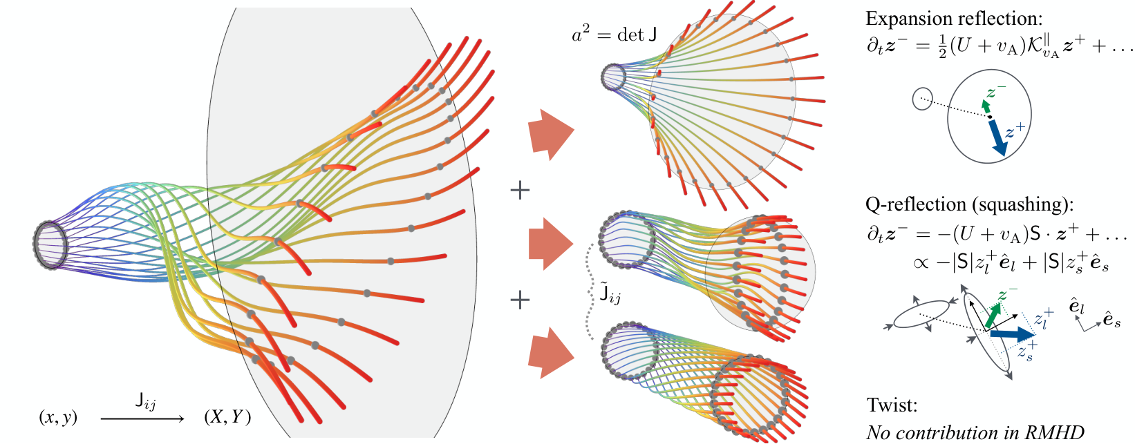
The term $\bm{z}^{\mp}\!\cdot\!\nabla\hat{\bm{b}}$ in (18) embodies the most general form of Alfvénic reflection. While this term has been written similarly in many previous works Zhou and Matthaeus 1990; Velli 1993, as far as we are aware its effects have only been considered for a flux tube that possesses axisymmetry about $\hat{\bm{b}}$, when it reduces to a “standard” reflection form $\bm{z}^{\mp}\nabla\cdot\hat{\bm{b}}/2$ (see below). Here, we detail its more general effects, which have interesting implications for coronal heating.

Because $\bm{z}^{\pm}\cdot\hat{\bm{b}}=0$, only the perpendicular part of the matrix $\nabla\hat{\bm{b}}$ enters (likewise, since $\nabla\hat{\bm{b}}\cdot\hat{\bm{b}}=0$, $\bm{z}^{\mp}\!\cdot\!\nabla\hat{\bm{b}}$ contributes only to the Alfvénic sector). We then define a locally field-aligned orthonormal basis $(\hat{\bm{e}}_{1},\hat{\bm{e}}_{2},\hat{\bm{b}})$ and write, without loss of generality,

where $\mathsf{I}_{\perp}$ is the $2\times 2$ identity in the perpendicular subspace, the traceless symmetric matrix $\mathsf{S}$ describes squashing of the flux tube into an ellipse, and the (traceless) antisymmetric matrix $\mathsf{A}=\hat{\bm{b}}\!\cdot\!\nabla\times\hat{\bm{b}}\;(\hat{\bm{e}}_{1}\hat{\bm{e}}_{2}-\hat{\bm{e}}_{2}\hat{\bm{e}}_{1})/2,$ encodes the twist of the field line. Their effects are illustrated graphically in fig. 4 and can be understood as follows:

1. (i)

   The isotropic piece, $(\nabla\!\cdot\!\hat{\bm{b}})\mathsf{I}_{\perp}/2$, reproduces the familiar “magnetic-expansion” reflection: using $\nabla\cdot\hat{\bm{b}}=-\mathcal{K}_{B}^{\|}$ this term combines with $\bm{z}^{\mp}\mathcal{K}_{\rho}^{\|}/4$ in eq. 18 to yield the reflection term $-(U\mp v_{\rm A})\mathcal{K}_{v_{\rm A}}^{\|}\bm{z}^{\mp}/2$. This matches the standard form (19), as appropriate under the assumption of a cylindrically symmetric flux tube with $\mathsf{S}=\mathsf{A}=0$.

2. (ii)

   The antisymmetric “twist” part does not contribute at RMHD order. This can be proven by taking its curl, which shows that $\bm{z}^{\mp}\!\cdot\!\mathsf{A}$ is a gradient of a scalar potential ¹¹ 1 The proof is straightforward using the potential form for $\bm{z}^{\pm}$. Compute $\nabla\times(\bm{z}^{+}\cdot\mathsf{A})=\nabla\times(\hat{\bm{b}}\times\nabla\zeta^{+}\cdot\mathsf{A})$, which gives $-\hat{\bm{b}}\,\mathsf{A}:\nabla\nabla\zeta^{+}$ to lowest order. The $\nabla\nabla$ operator is symmetric, showing that $\mathsf{A}:\nabla\nabla\zeta^{+}=0$, and thus that $\bm{z}^{+}\cdot\mathcal{A}$ is a purely compressive perpendicular forcing on $\bm{z}^{-}$. . Any such gradient contribution is automatically cancelled by the perpendicular pressure force that enforces $\nabla\cdot\bm{z}^{\pm}=0$ and so cannot drive significant reflection (equivalently, the term will not appear in the potential form of the equations (147)).

3. (iii)

   The symmetric‐traceless tensor $\mathsf{S}$ survives and represents reflection caused by area-preserving elliptical deformations of the flux surface. By rotating into its local eigenbasis, $\hat{\bm{e}}_{l}$ and $\hat{\bm{e}}_{s}$, which are mutually perpendicular directions lying along the long and short axis of the ellipse, respectively, $\mathsf{S}$ becomes $\mathsf{S}=\mathrm{diag}(|\mathsf{S}|,-|\mathsf{S}|)$, where $|\mathsf{S}|=({\mathsf{S}_{ij}\mathsf{S}_{ij}}/2)^{1/2}$ is the rate at which the long axis becomes longer (i.e., $\pm|\mathsf{S}|$ are the eigenvalues of $\mathsf{S}$). Then $\bm{z}^{\mp}\cdot\mathsf{S}=|\mathsf{S}|z^{\mp}_{l}\,\hat{\bm{e}}_{l}-|\mathsf{S}|z^{\mp}_{s}\,\hat{\bm{e}}_{s}$, i.e., the long-axis component of $\bm{z}^{\pm}$ reflects with the opposite sign to the short-axis component. Although this will change the correlation of the forced $\bm{z}^{-}$ with the driving $\bm{z}^{+}$ compared to conventional RDT Perez et al. 2021; Meyrand et al. 2025; Bowen et al. 2025, it is still expected to inject energy into $\bm{z}^{\mp}$ at a rate comparable to the isotropic expansion term if $|\mathsf{S}|$ and $\nabla\cdot\hat{\bm{b}}$ are comparable.

Collecting the non-vanishing pieces, the net Alfvénic reflection forcing reads

which will generally act as the primary driver of $\bm{z}^{-}$ in the solar context (see section III). The first term is standard non-WKB reflection, while the second represents reflection by flux-surface squashing — absent in straight-tube models but potentially dominant in regions where field lines become tangled. A quantitative estimate of its contribution to heating, in particular the relation to the measured “squashing factor” $\mathcal{Q}$ from PFSS models, is deferred to section III.

Dotting Eqs. (18), (22), (23), and (24) with $\bm{z}^{\pm}$, $\delta{u}_{\|}$, $\delta{\tilde{V}}_{\|}$, and $\delta s$, respectively, then taking the turbulent average, one finds the the generalized RMHD quadratic free-energy invariant. This is most naturally written in terms of the Alfvénic, slow-mode, and entropy-mode energies:

respectively. Their sum

is the fluctuation’s contribution to the second-order perturbation of the total MHD energy density,

where $E_{\rm th}={p}/(\gamma-1)$. The compressive pieces combine so that $W^{\|}_{+}+W^{\|}_{-}+W_{s}$ contains both the quadratic correction to $E_{\rm th}$ and the kinetic and magnetic energies of slow-mode fluctuations.

The evolution of $W^{\rm tot}$ obeys a conservation law,

where $v_{\rm wave}=\{\pm v_{\rm A},\pm v_{S},0\}$ for $W_{\rm wave}=\{W^{\pm}_{\perp},W^{\pm}_{\|},W_{s}\}$, and $D^{\rm tot}$ is the positive-definite function encoding the fluctuation’s dissipation (164). Note that the (fast) time derivative has disappeared from (31) due to the application of the intermediate-time average as part of the turbulent average, encoding physically the idea that fluctuations sit in quasi-steady balance between propagation, forcing, and dissipation.

The perpendicular source $\mathcal{Y}^{\perp}$ can be written as a sum of five contributions,

where $\bm{U}_{\perp 2}$ is a second-order perpendicular mean flow, which is set up by the fluctuations in order to maintain perpendicular force balance (its properties are discussed in App. A.5.9, but it does not feature heavily in the core theory). The individual sources are

where

(defining $\bm{V}_{\!p}$ for later use), and

The quantities $\bm{V}_{\!U}$, $\widetilde{\bm{V}}_{\!\psi}$, $\widetilde{\bm{V}}_{\!\rho}$, and $\widetilde{\bm{V}}_{\!p}$ will soon be identified as the turbulent transport velocities of $\bm{U}$, $\bm{B}$, $\rho$, and $p$, respectively. Note that adding the contributions in $\mathcal{Y}^{\perp}$ cancels $\bm{U}_{\perp 2}$ via the equilibrium condition (12), explaining its lack of appearance in the fluctuation equations (this organization of terms will be clarified below).

The terms $\mathcal{Y}^{\perp}_{U}$, $\mathcal{Y}^{\perp}_{B}$, and $\mathcal{Y}^{\perp}_{g}$ describe exchange between the fluctuations and the free energy stored in, respectively, background kinetic energy, magnetic energy, and effective gravitational potential energy, while $\mathcal{Y}^{\perp}_{\rm th}$ describes exchange with background density and temperature gradients (equivalently, pressure and entropy gradients). The parallel contribution $\mathcal{Y}^{\|}$ encodes the wave-mean energy exchange, via pressure work and Reynolds–Maxwell stresses, as the waves propagate along an inhomogeneous background. It is given explicitly in eqs. 166 and 167 (split into its Alfvénic $\mathcal{Y}^{\|}_{\rm A}$ and compressive $\mathcal{Y}^{\|}_{C}$ contributions), generalizing well-known wave “work” terms Chandran et al. 2015; Perez et al. 2021 to compressive fluctuations and a general background.

In the homogeneous RMHD limit Schekochihin et al. 2009, all background gradients and curvature vanish, so $\mathcal{Y}^{\perp}=\mathcal{Y}^{\|}=0$ and each of the five energies $W^{\pm}_{\perp}$, $W^{\pm}_{\|}$, and $W_{s}$ are individually conserved, simply moving along $\hat{\bm{b}}$ at speed $U+v_{\rm wave}$.

References

- Velli et al. (1989) M. Velli, R. Grappin, and A. Mangeney, Phys. Rev. Lett. 63, 1807 (1989).
- Spitkovsky (2006) A. Spitkovsky, Astrophys. J. Lett. 648, L51 (2006), arXiv:astro-ph/0603147 [astro-ph] .
- Parker (1966) E. N. Parker, Astrophys. J. 145, 811 (1966).
- Shu (1974) F. H. Shu, Astron. Astro. 33, 55 (1974).
- Weber and Davis (1967) E. J. Weber and J. Davis, Leverett, Astrophys. J. 148, 217 (1967).
- Mestel (1968) L. Mestel, Mon. Not. R. Astron. Soc. 140, 177 (1968).
- Parker (1958) E. N. Parker, Astrophys. J. 128, 664 (1958).
- Cranmer and Winebarger (2019) S. R. Cranmer and A. R. Winebarger, Ann. Rev. Astron. Astrophys. 57, 157 (2019), arXiv:1811.00461 [astro-ph.SR] .
- Viall and Borovsky (2020) N. M. Viall and J. E. Borovsky, J. Geophys. Res. Space Phys. 125, e26005 (2020).
- Klimchuk (2015) J. A. Klimchuk, Proc. R. Soc. A 373, 20140256 (2015).
- De Moortel and Browning (2015) I. De Moortel and P. Browning, Proc. R. Soc. A 373, 20140269 (2015).
- Reale (2014) F. Reale, Living Rev. Solar Phys. 11, 4 (2014).
- Cranmer et al. (2009) S. R. Cranmer, W. H. Matthaeus, B. A. Breech, and J. C. Kasper, Astrophys. J. 702, 1604 (2009), arXiv:0907.2650 [astro-ph.SR] .
- Parker (1988) E. N. Parker, Astrophys. J. 330, 474 (1988).
- DeForest (2007) C. E. DeForest, Astrophys. J. 661, 532 (2007), arXiv:astro-ph/0610178 [astro-ph] .
- Tomczyk et al. (2007) S. Tomczyk, S. W. McIntosh, S. L. Keil, P. G. Judge, T. Schad, D. H. Seeley, and J. Edmondson, Science 317, 1192 (2007).
- Chitta et al. (2020) L. P. Chitta, H. Peter, E. R. Priest, and S. K. Solanki, Astron. Astro. 644, A130 (2020), arXiv:2010.12560 [astro-ph.SR] .
- Chen et al. (2016) C. H. K. Chen, L. Matteini, A. A. Schekochihin, M. L. Stevens, C. S. Salem, B. A. Maruca, M. W. Kunz, and S. D. Bale, Astrophys. J. 825, 1 (2016).
- McComas et al. (2000) D. J. McComas, B. L. Barraclough, H. O. Funsten, J. T. Gosling, E. Santiago-Muñoz, R. M. Skoug, B. E. Goldstein, M. Neugebauer, P. Riley, and A. Balogh, J. Geophys. Res. 105, 10419 (2000).
- Cranmer et al. (2007) S. R. Cranmer, A. A. van Ballegooijen, and R. J. Edgar, Astrophys. J. Supp. 171, 520 (2007), arXiv:astro-ph/0703333 [astro-ph] .
- Hollweg (1986) J. V. Hollweg, J. Geophys. Res. 91, 4111 (1986).
- Matthaeus et al. (1999) W. H. Matthaeus, G. P. Zank, S. Oughton, D. J. Mullan, and P. Dmitruk, Astrophys. J. Lett. 523, L93 (1999).
- Verdini et al. (2009) A. Verdini, M. Velli, and E. Buchlin, Astrophys. J. Lett. 700, L39 (2009), arXiv:0905.2618 [astro-ph.SR] .
- van Ballegooijen and Asgari-Targhi (2016) A. A. van Ballegooijen and M. Asgari-Targhi, Astrophys. J. 821, 106 (2016), arXiv:1602.06883 [astro-ph.SR] .
- Shoda et al. (2019) M. Shoda, T. K. Suzuki, M. Asgari-Targhi, and T. Yokoyama, Astrophys. J. Lett. 880, L2 (2019), arXiv:1905.11685 [astro-ph.SR] .
- Chandran and Perez (2019) B. D. G. Chandran and J. C. Perez, J. Plasma Phys. 85, 905850409 (2019), arXiv:1908.00880 [physics.space-ph] .
- Sioulas et al. (2025) N. Sioulas, M. Velli, C. Shi, T. A. Bowen, A. Mallet, A. Verdini, B. D. G. Chandran, A. Tenerani, J.-B. Dakeyo, S. D. Bale, D. Larson, J. S. Halekas, L. Matteini, V. Réville, C. H. K. Chen, O. M. Romeo, M. Liu, R. Livi, A. Rahmati, and P. L. Whittlesey, arXiv e-prints , arXiv:2510.10106 (2025), arXiv:2510.10106 [astro-ph.SR] .
- Wang and Sheeley (1990) Y. M. Wang and J. Sheeley, N. R., Astrophys. J. 355, 726 (1990).
- Arge and Pizzo (2000) C. N. Arge and V. J. Pizzo, J. Geophys. Res. 105, 10465 (2000).
- MacNeice et al. (2018) P. MacNeice, L. K. Jian, S. K. Antiochos, C. N. Arge, C. D. Bussy-Virat, M. L. DeRosa, B. V. Jackson, J. A. Linker, Z. Mikic, M. J. Owens, A. J. Ridley, P. Riley, N. Savani, and I. Sokolov, Space Weather 16, 1644 (2018).
- Elliott et al. (2022) H. A. Elliott, C. N. Arge, C. J. Henney, M. A. Dayeh, G. Livadiotis, J.-M. Jahn, and C. E. DeForest, Space Weather 20, e2021SW002868 (2022).
- Downs et al. (2016) C. Downs, R. Lionello, Z. Mikić, J. A. Linker, and M. Velli, Astrophys. J. 832, 180 (2016), arXiv:1610.02113 [astro-ph.SR] .
- Morton et al. (2023) R. J. Morton, R. Sharma, E. Tajfirouze, and H. Miriyala, Rev. Modern Plasma Phys. 7, 17 (2023), arXiv:2208.05222 [astro-ph.SR] .
- Lee and Roberts (1986) M. A. Lee and B. Roberts, Astrophys. J. 301, 430 (1986).
- Davila (1987) J. M. Davila, Astrophys. J. 317, 514 (1987).
- Magyar et al. (2019a) N. Magyar, T. Van Doorsselaere, and M. Goossens, Astrophys. J. 882, 50 (2019a), arXiv:1907.10408 [astro-ph.SR] .
- Southwood and Saunders (1985) D. J. Southwood and M. A. Saunders, Planet. Space Sci. 33, 127 (1985).
- Similon and Sudan (1989) P. L. Similon and R. N. Sudan, Astrophys. J. 336, 442 (1989).
- Heyvaerts and Priest (1983) J. Heyvaerts and E. R. Priest, Astron. Astro. 117, 220 (1983).
- Van Doorsselaere et al. (2020) T. Van Doorsselaere, A. K. Srivastava, P. Antolin, N. Magyar, S. Vasheghani Farahani, H. Tian, D. Kolotkov, L. Ofman, M. Guo, I. Arregui, I. De Moortel, and D. Pascoe, Space Sci. Rev. 216, 140 (2020), arXiv:2012.01371 [astro-ph.SR] .
- Callen et al. (2010) J. D. Callen, C. C. Hegna, and A. J. Cole, Phys. Plasmas 17, 056113 (2010).
- Barnes et al. (2010) M. Barnes, I. G. Abel, W. Dorland, T. Görler, G. W. Hammett, and F. Jenko, Physics of Plasmas 17, 056109 (2010), arXiv:0912.1974 [physics.plasm-ph] .
- Abel et al. (2013) I. G. Abel, G. G. Plunk, E. Wang, M. Barnes, S. C. Cowley, W. Dorland, and A. A. Schekochihin, Reports on Progress in Physics 76, 116201 (2013), arXiv:1209.4782 [physics.plasm-ph] .
- Jenko et al. (2000) F. Jenko, W. Dorland, M. Kotschenreuther, and B. N. Rogers, Phys. Plasmas 7, 1904 (2000).
- Candy et al. (2009) J. Candy, C. Holland, R. E. Waltz, M. R. Fahey, and E. Belli, Phys. Plasmas 16, 060704 (2009).
- Citrin et al. (2017) J. Citrin, C. Bourdelle, F. J. Casson, C. Angioni, N. Bonanomi, Y. Camenen, X. Garbet, L. Garzotti, T. Görler, O. Gürcan, F. Koechl, F. Imbeaux, O. Linder, K. van de Plassche, P. Strand, G. Szepesi, and J. Contributors, Plasma Phys. Control. Fusion 59, 124005 (2017), arXiv:1708.01224 [physics.plasm-ph] .
- Titov et al. (2002) V. S. Titov, G. Hornig, and P. Démoulin, J. Geophys. Res. Space Phys. 107, 1164 (2002).
- Antiochos et al. (2011) S. K. Antiochos, Z. Mikić, V. S. Titov, R. Lionello, and J. A. Linker, Astrophys. J. 731, 112 (2011), arXiv:1102.3704 [astro-ph.SR] .
- Zank et al. (1996) G. P. Zank, W. H. Matthaeus, and C. W. Smith, J. Geophys. Res. 101, 17093 (1996).
- Oughton et al. (2011) S. Oughton, W. H. Matthaeus, C. W. Smith, B. Breech, and P. A. Isenberg, J. Geophys. Res. Space Phys. 116, A08105 (2011).
- Breech et al. (2008) B. Breech, W. H. Matthaeus, J. Minnie, J. W. Bieber, S. Oughton, C. W. Smith, and P. A. Isenberg, J. Geophys. Res. Space Phys. 113, A08105 (2008).
- Usmanov et al. (2018) A. V. Usmanov, W. H. Matthaeus, M. L. Goldstein, and R. Chhiber, Astrophys. J. 865, 25 (2018).
- Zank et al. (2017) G. P. Zank, L. Adhikari, P. Hunana, D. Shiota, R. Bruno, and D. Telloni, Astrophys. J. 835, 147 (2017).
- Leer and Holzer (1980) E. Leer and T. E. Holzer, J. Geophys. Res. 85, 4681 (1980).
- Hansteen and Leer (1995) V. H. Hansteen and E. Leer, J. Geophys. Res. 100, 21577 (1995).
- Chandran (2021) B. D. G. Chandran, J. Plasma Phys. 87, 905870304 (2021), arXiv:2101.04156 [astro-ph.SR] .
- van der Holst et al. (2014) B. van der Holst, I. V. Sokolov, X. Meng, M. Jin, W. B. Manchester, IV, G. Tóth, and T. I. Gombosi, Astrophys. J. 782, 81 (2014), arXiv:1311.4093 [astro-ph.SR] .
- Mikić et al. (2018) Z. Mikić, C. Downs, J. A. Linker, R. M. Caplan, D. H. Mackay, L. A. Upton, P. Riley, R. Lionello, T. Török, V. S. Titov, J. Wijaya, M. Druckmüller, J. M. Pasachoff, and W. Carlos, Nature Astron. 2, 913 (2018).
- Owens et al. (2005) M. J. Owens, C. N. Arge, H. E. Spence, and A. Pembroke, J. Geophys. Res. Space Phys. 110, A12105 (2005).
- Sokolov et al. (2021) I. V. Sokolov, B. v. d. Holst, W. B. Manchester, D. C. Su Ozturk, J. Szente, A. Taktakishvili, G. Tóth, M. Jin, and T. I. Gombosi, Astrophys. J. 908, 172 (2021), arXiv:1609.04379 [astro-ph.SR] .
- Parenti et al. (2022) S. Parenti, V. Réville, A. S. Brun, R. F. Pinto, F. Auchère, E. Buchlin, B. Perri, and A. Strugarek, Astrophys. J. 929, 75 (2022), arXiv:2203.10876 [astro-ph.SR] .
- Réville et al. (2022) V. Réville, N. Fargette, A. P. Rouillard, B. Lavraud, M. Velli, A. Strugarek, S. Parenti, A. S. Brun, C. Shi, A. Kouloumvakos, N. Poirier, R. F. Pinto, P. Louarn, A. Fedorov, C. J. Owen, V. Génot, T. S. Horbury, R. Laker, H. O’Brien, V. Angelini, E. Fauchon-Jones, and J. C. Kasper, Astron. Astro. 659, A110 (2022), arXiv:2112.07445 [astro-ph.SR] .
- Chhiber et al. (2021) R. Chhiber, A. V. Usmanov, W. H. Matthaeus, and M. L. Goldstein, Astrophys. J. 923, 89 (2021), arXiv:2107.11657 [physics.space-ph] .
- Citrin et al. (2022) J. Citrin, S. Maeyama, C. Angioni, N. Bonanomi, C. Bourdelle, F. J. Casson, E. Fable, T. Görler, P. Mantica, A. Mariani, M. Sertoli, G. Staebler, T. Watanabe, and JET Contributors, Nuclear Fusion 62, 086025 (2022), arXiv:2209.09683 [physics.plasm-ph] .
- Kawazura et al. (2022) Y. Kawazura, A. A. Schekochihin, M. Barnes, W. Dorland, and S. A. Balbus, J. Plasma Phys. 88, 905880311 (2022), arXiv:2110.12434 [astro-ph.HE] .
- Dmitruk et al. (2002) P. Dmitruk, W. H. Matthaeus, L. J. Milano, S. Oughton, G. P. Zank, and D. J. Mullan, Astrophys. J. 575, 571 (2002), arXiv:astro-ph/0204347 [astro-ph] .
- Banaszkiewicz et al. (1998) M. Banaszkiewicz, W. I. Axford, and J. F. McKenzie, Astron. Astro. 337, 940 (1998).
- Frieman and Chen (1982) E. A. Frieman and L. Chen, Phys. Fluids 25, 502 (1982).
- Schekochihin et al. (2009) A. A. Schekochihin, S. C. Cowley, W. Dorland, G. W. Hammett, G. G. Howes, E. Quataert, and T. Tatsuno, Astrophys. J. Supp. 182, 310 (2009).
- Chandran and Hollweg (2009) B. D. G. Chandran and J. V. Hollweg, Astrophys. J. 707, 1659 (2009), arXiv:0911.1068 [astro-ph.SR] .
- Wang et al. (2022) B.-B. Wang, G. P. Zank, L. Adhikari, and L.-L. Zhao, Astrophys. J. 928, 176 (2022), arXiv:2111.11096 [physics.plasm-ph] .
- Jacques (1978) S. A. Jacques, Astrophys. J. 226, 632 (1978).
- Cranmer et al. (2017) S. R. Cranmer, S. E. Gibson, and P. Riley, Space Sci. Rev. 212, 1345 (2017), arXiv:1708.07169 [astro-ph.SR] .
- Barnes and Hollweg (1974) A. Barnes and J. V. Hollweg, J. Geophys. Res. 79, 2302 (1974).
- Hollweg (1974) J. V. Hollweg, J. Geophys. Res. 79, 1539 (1974).
- Whang (1980) Y. C. Whang, J. Geophys. Res. 85, 2285 (1980).
- Zhou and Matthaeus (1990) Y. Zhou and W. H. Matthaeus, J. Geophys. Res. 95, 10291 (1990).
- Velli (1993) M. Velli, Astron. Astro. 270, 304 (1993).
- Cranmer (2005) S. R. Cranmer, in Solar Wind 11/SOHO 16, Connecting Sun and Heliosphere, ESA Special Publication, Vol. 592, edited by B. Fleck, T. H. Zurbuchen, and H. Lacoste (2005) p. 159, arXiv:astro-ph/0506508 [astro-ph] .
- David et al. (2025) V. David, B. D. G. Chandran, R. Meyrand, J. Squire, and E. L. Yerger, J. Plasma Phys. 91, E68 (2025), arXiv:2501.17702 [physics.plasm-ph] .
- Magyar et al. (2019b) N. Magyar, T. Van Doorsselaere, and M. Goossens, Astrophys. J. 873, 56 (2019b), arXiv:1902.01619 [astro-ph.SR] .
- Lithwick and Goldreich (2001) Y. Lithwick and P. Goldreich, Astrophys. J. 562, 279 (2001).
- Heinemann and Olbert (1980) M. Heinemann and S. Olbert, J. Geophys. Res. 85, 1311 (1980).
- (84) The proof is straightforward using the potential form for . Compute , which gives to lowest order. The operator is symmetric, showing that , and thus that is a purely compressive perpendicular forcing on .
- Perez et al. (2021) J. C. Perez, B. D. G. Chandran, K. G. Klein, and M. M. Martinović, J. Plasma Phys. 87, 905870218 (2021), arXiv:2103.09365 [astro-ph.SR] .
- Meyrand et al. (2025) R. Meyrand, J. Squire, A. Mallet, and B. D. G. Chandran, J. Plasma Phys. 91, E29 (2025), arXiv:2308.10389 [astro-ph.SR] .
- Bowen et al. (2025) T. A. Bowen, C. I. Dunn, A. Mallet, J. Squire, S. T. Badman, S. D. Bale, T. Dudok de Wit, T. S. Horbury, K. G. Klein, D. Larson, L. Matteini, M. D. McManus, and N. Sioulas, Astrophys. J. 985, 49 (2025), arXiv:2110.11454 [physics.plasm-ph] .
- Chandran et al. (2015) B. D. G. Chandran, J. C. Perez, D. Verscharen, K. G. Klein, and A. Mallet, Astrophys. J. 811, 50 (2015), arXiv:1509.01135 [astro-ph.SR] .
- Chew et al. (1956) C. F. Chew, M. L. Goldberger, and F. E. Low, Proc. R. Soc. London A 236, 112 (1956).
- Kulsrud (1983) R. M. Kulsrud, in Handbook of Plasma Physics, edited by R. N. Sagdeev and M. N. Rosenbluth (Princeton University Press, 1983).
- Foote and Kulsrud (1979) E. A. Foote and R. M. Kulsrud, Astrophys. J. 233, 302 (1979).
- Kunz et al. (2015) M. W. Kunz, A. A. Schekochihin, C. H. K. Chen, I. G. Abel, and S. C. Cowley, J. Plasma Phys. 81, 325810501 (2015).
- Snyder et al. (1997) P. B. Snyder, G. W. Hammett, and W. Dorland, Phys. Plasmas 4, 3974 (1997).
- Schekochihin et al. (2016) A. A. Schekochihin, J. T. Parker, E. G. Highcock, P. J. Dellar, W. Dorland, and G. W. Hammett, J. Plasma Phys. 82, 905820212 (2016), arXiv:1508.05988 [physics.plasm-ph] .
- Meyrand et al. (2019) R. Meyrand, A. Kanekar, W. Dorland, and A. A. Schekochihin, Proc. Nat. Acad. Sci. 116, 1185 (2019), arXiv:1808.04284 [physics.plasm-ph] .
- Kunz et al. (2014) M. W. Kunz, A. A. Schekochihin, and J. M. Stone, Phys. Rev. Lett. 112, 205003 (2014).
- Verscharen et al. (2017) D. Verscharen, C. H. K. Chen, and R. T. Wicks, Astrophys. J. 840, 106 (2017), arXiv:1703.03040 [physics.space-ph] .
- Squire et al. (2019) J. Squire, A. A. Schekochihin, E. Quataert, and M. W. Kunz, J. Plasma Phys. 85, 905850114 (2019).
- Squire et al. (2023a) J. Squire, M. W. Kunz, L. Arzamasskiy, Z. Johnston, E. Quataert, and A. A. Schekochihin, J. Plasma Phys. 89, 905890417 (2023a), arXiv:2303.00468 [astro-ph.HE] .
- Majeski et al. (2024) S. Majeski, M. W. Kunz, and J. Squire, J. Plasma Phys. 90, 535900601 (2024), arXiv:2405.02418 [astro-ph.HE] .
- Bale et al. (2019) S. D. Bale, S. T. Badman, J. W. Bonnell, T. A. Bowen, D. Burgess, A. W. Case, C. A. Cattell, B. D. G. Chandran, C. C. Chaston, C. H. K. Chen, J. F. Drake, T. D. de Wit, et al., Nature 576, 237 (2019).
- Squire et al. (2020) J. Squire, B. D. G. Chandran, and R. Meyrand, Astrophys. J. Lett. 891, L2 (2020), arXiv:2001.08422 [physics.space-ph] .
- Dmitruk et al. (2005) P. Dmitruk, W. H. Matthaeus, and S. Oughton, Phys. Plasmas 12, 112304 (2005).
- Abbas and Squire (2026) K. Abbas and J. Squire, J. Plasma Phys. 92, E55 (2026).
- Mallet et al. (2021) A. Mallet, J. Squire, B. D. G. Chandran, T. Bowen, and S. D. Bale, Astrophys. J. 918, 62 (2021).
- Johnston et al. (2022) Z. Johnston, J. Squire, A. Mallet, and R. Meyrand, Phys. Plasmas 29, 072902 (2022), arXiv:2205.09446 [astro-ph.SR] .
- Kiyani et al. (2015) K. H. Kiyani, K. T. Osman, and S. C. Chapman, Phil. Trans. Roy. Soc. A 373, 20140155 (2015).
- Meyrand et al. (2021) R. Meyrand, J. Squire, A. A. Schekochihin, and W. Dorland, J. Plasma Phys. 87, 535870301 (2021), arXiv:2009.02828 [physics.space-ph] .
- Squire et al. (2022) J. Squire, R. Meyrand, M. W. Kunz, L. Arzamasskiy, A. A. Schekochihin, and E. Quataert, Nature Astron. 6, 715 (2022), arXiv:2109.03255 [astro-ph.SR] .
- Squire et al. (2023b) J. Squire, R. Meyrand, and M. W. Kunz, Astrophys. J. Lett. 957, L30 (2023b), arXiv:2308.13048 [astro-ph.SR] .
- Adkins et al. (2025) T. Adkins, R. Meyrand, and J. Squire, Astrophys. J. 990, 138 (2025), arXiv:2504.16177 [physics.plasm-ph] .
- Johnston et al. (2025) Z. Johnston, J. Squire, and R. Meyrand, Phys. Rev. Lett. 135, 095201 (2025), arXiv:2409.07015 [astro-ph.SR] .
- Zhang et al. (2025) M. F. Zhang, M. W. Kunz, J. Squire, and K. G. Klein, Astrophys. J. 979, 121 (2025), arXiv:2408.04703 [astro-ph.SR] .
- Zocco and Schekochihin (2011) A. Zocco and A. A. Schekochihin, Phys. Plasmas 18, 102309 (2011), arXiv:1104.4622 [physics.plasm-ph] .
- Schekochihin et al. (2019) A. A. Schekochihin, Y. Kawazura, and M. A. Barnes, J. Plasma Phys. 85, 905850303 (2019), arXiv:1812.09792 [physics.plasm-ph] .
- Adkins et al. (2024) T. Adkins, R. Meyrand, and J. Squire, J. Plasma Phys. 90, 905900403 (2024), arXiv:2404.09380 [physics.plasm-ph] .
- van Ballegooijen et al. (2011) A. A. van Ballegooijen, M. Asgari-Targhi, S. R. Cranmer, and E. E. DeLuca, Astrophys. J. 736, 3 (2011), arXiv:1105.0402 [astro-ph.SR] .
- Perez and Chandran (2013) J. C. Perez and B. D. G. Chandran, Astrophys. J. 776, 124 (2013).
- van Ballegooijen et al. (2017) A. A. van Ballegooijen, M. Asgari-Targhi, and A. Voss, Astrophys. J. 849, 46 (2017), arXiv:1710.05074 [astro-ph.SR] .
- Sachdeva et al. (2019) N. Sachdeva, B. van der Holst, W. B. Manchester, G. Tóth, Y. Chen, D. G. Lloveras, A. M. Vásquez, P. Lamy, J. Wojak, B. V. Jackson, H.-S. Yu, and C. J. Henney, Astrophys. J. 887, 83 (2019), arXiv:1910.08110 [astro-ph.SR] .
- Ionson (1978) J. A. Ionson, Astrophys. J. 226, 650 (1978).
- Wicks et al. (2013) R. T. Wicks, A. Mallet, T. S. Horbury, C. H. K. Chen, A. A. Schekochihin, and J. J. Mitchell, Phys. Rev. Lett. 110, 025003 (2013), arXiv:1209.5362 [physics.space-ph] .
- Schekochihin (2022) A. A. Schekochihin, J. Plasma Phys. 88, 155880501 (2022), arXiv:2010.00699 [physics.plasm-ph] .
- Barnes et al. (2011) M. Barnes, F. I. Parra, and A. A. Schekochihin, Phys. Rev. Lett. 107, 115003 (2011), arXiv:1104.4514 [physics.plasm-ph] .
- Adkins et al. (2022) T. Adkins, A. A. Schekochihin, P. G. Ivanov, and C. M. Roach, J. Plasma Phys. 88, 905880410 (2022), arXiv:2201.05670 [physics.plasm-ph] .
- Adkins et al. (2026) T. Adkins, I. G. Abel, M. Barnes, S. Buller, W. Dorland, P. G. Ivanov, R. Meyrand, F. I. Parra, A. A. Schekochihin, and J. Squire, arXiv e-prints , arXiv:2601.15391 (2026), arXiv:2601.15391 [physics.plasm-ph] .
- (127) Advection by the magnetic field in the compressive equations accounts for propagation of fluctuations along the true (wandering) field lines caused by fluctuations. Field-line tangling will generate small perpendicular scales and thus act as an effective cascade in both and (the latter via reconnection of field lines enabled by dissipation Meyrand et al. 2019). If such terms dominate, then the interpretation of Eqs. (45) must be modified, with, for example, becoming more relevant to , and vice versa. In the slow-mode equations, the ratio of this advection to that from is for , or for , and since at , the effect should be subdominant in the corona for at least one of and . Since we generally care about whichever of and is larger, this justifies its neglect. In the equation, perpendicular advection yields a turbulent balance for rather than , with the interpretation that parallel compressions locally balance forcing, meaning (47) remains an appropriate estimate for .
- Verdini and Velli (2007) A. Verdini and M. Velli, Astrophys. J. 662, 669 (2007), arXiv:astro-ph/0702205 [astro-ph] .
- Goldreich and Sridhar (1995) P. Goldreich and S. Sridhar, Astrophys. J. 438, 763 (1995).
- Usmanov et al. (2014) A. V. Usmanov, M. L. Goldstein, and W. H. Matthaeus, Astrophys. J. 788, 43 (2014).
- Réville et al. (2020) V. Réville, M. Velli, O. Panasenco, A. Tenerani, C. Shi, S. T. Badman, S. D. Bale, J. C. Kasper, M. L. Stevens, K. E. Korreck, J. W. Bonnell, A. W. Case, T. D. de Wit, K. Goetz, P. R. Harvey, D. E. Larson, R. Livi, D. M. Malaspina, R. J. MacDowall, M. Pulupa, and P. L. Whittlesey, Astrophys. J. Supp. 246, 24 (2020).
- Bruno and Carbone (2013) R. Bruno and V. Carbone, Living Rev. Solar Phys. 10, 2 (2013).
- Jenko and Dorland (2002) F. Jenko and W. Dorland, Phys. Rev. Lett. 89, 225001 (2002).
- Garbet et al. (2010) X. Garbet, Y. Idomura, L. Villard, and T. H. Watanabe, Nuclear Fusion 50, 043002 (2010).
- Boxer et al. (2010) A. C. Boxer, R. Bergmann, J. L. Ellsworth, D. T. Garnier, J. Kesner, M. E. Mauel, and P. Woskov, Nature Phys. 6, 207 (2010).
- Hasegawa (1987) A. Hasegawa, Comments Plasma Phys. Controlled Fusion 11, 147 (1987).
- Kouznetsov et al. (2007) A. Kouznetsov, J. P. Freidberg, and J. Kesner, Phys. Plasmas 14, 102502 (2007).
- Kobayashi et al. (2010) S. Kobayashi, B. N. Rogers, and W. Dorland, Phys. Rev. Lett. 105, 235004 (2010).
- Bale et al. (2021) S. D. Bale, T. S. Horbury, M. Velli, M. I. Desai, J. S. Halekas, M. D. McManus, O. Panasenco, S. T. Badman, T. A. Bowen, B. D. G. Chandran, J. F. Drake, J. C. Kasper, R. Laker, A. Mallet, L. Matteini, T. D. Phan, N. E. Raouafi, J. Squire, L. D. Woodham, and T. Woolley, Astrophys. J. 923, 174 (2021), arXiv:2109.01069 [astro-ph.SR] .
- Nies et al. (2026) R. Nies, F. Parra, M. Barnes, N. Mandell, and W. Dorland, Phys. Rev. Research 8, 013295 (2026), arXiv:2409.02283 [physics.plasm-ph] .
- Lionello et al. (2014) R. Lionello, M. Velli, C. Downs, J. A. Linker, and Z. Mikić, Astrophys. J. 796, 111 (2014).
- Raymond et al. (2014) J. C. Raymond, P. I. McCauley, S. R. Cranmer, and C. Downs, Astrophys. J. 788, 152 (2014), arXiv:1405.1639 [astro-ph.SR] .
- Lionello et al. (2009) R. Lionello, J. A. Linker, and Z. Mikić, Astrophys. J. 690, 902 (2009).
- Vásquez et al. (2003) A. M. Vásquez, A. A. van Ballegooijen, and J. C. Raymond, Astrophys. J. 598, 1361 (2003), arXiv:astro-ph/0310846 [astro-ph] .
- Gary (2001) G. A. Gary, Solar Phys 203, 71 (2001).
- Mancuso et al. (2003) S. Mancuso, J. C. Raymond, J. Kohl, Y.-K. Ko, M. Uzzo, and R. Wu, Astron. Astro. 400, 347 (2003).
- Barkhudarov (1991) M. R. Barkhudarov, Solar Phys. 135, 131 (1991).
- Huang et al. (2023) Z. Huang, N. Sioulas, C. Shi, M. Velli, T. Bowen, N. Davis, B. D. G. Chandran, L. Matteini, N. Kang, X. Shi, J. Huang, S. D. Bale, J. C. Kasper, D. E. Larson, R. Livi, P. L. Whittlesey, A. Rahmati, K. Paulson, M. Stevens, A. W. Case, T. D. de Wit, D. M. Malaspina, J. W. Bonnell, K. Goetz, P. R. Harvey, and R. J. MacDowall, Astrophys. J. Lett. 950, L8 (2023), arXiv:2303.00843 [astro-ph.SR] .
- Klimchuk (2006) J. A. Klimchuk, Solar Phys. 234, 41 (2006), arXiv:astro-ph/0511841 [astro-ph] .
- Evans et al. (2012) R. M. Evans, M. Opher, R. Oran, B. van der Holst, I. V. Sokolov, R. Frazin, T. I. Gombosi, and A. Vásquez, Astrophys. J. 756, 155 (2012).
- Abbo et al. (2016) L. Abbo, L. Ofman, S. K. Antiochos, V. H. Hansteen, L. Harra, Y. K. Ko, G. Lapenta, B. Li, P. Riley, L. Strachan, R. von Steiger, and Y. M. Wang, Space Sci. Rev. 201, 55 (2016).
- Fargette et al. (2021) N. Fargette, B. Lavraud, A. P. Rouillard, V. Réville, T. Dudok De Wit, C. Froment, J. S. Halekas, T. D. Phan, D. M. Malaspina, S. D. Bale, J. C. Kasper, P. Louarn, A. W. Case, K. E. Korreck, D. E. Larson, M. Pulupa, M. L. Stevens, P. L. Whittlesey, and M. Berthomier, Astrophys. J. 919, 96 (2021), arXiv:2109.01519 [astro-ph.SR] .
- Horbury et al. (2023) T. S. Horbury, S. D. Bale, M. D. McManus, D. Larson, J. C. Kasper, R. Laker, L. Matteini, N. E. Raouafi, M. Velli, L. D. Woodham, T. Woolley, A. Fedorov, P. Louarn, R. Kieokaew, T. Durovcova, B. Chandran, and C. J. Owen, Phys. Plasmas 30, 082905 (2023).
- Roberts et al. (1987) D. A. Roberts, M. L. Goldstein, L. W. Klein, and W. H. Matthaeus, J. Geophys. Res. 92, 12023 (1987).
- Roberts et al. (1992) D. A. Roberts, M. L. Goldstein, W. H. Matthaeus, and S. Ghosh, J. Geophys. Res. 97, 17115 (1992).
- Chandrasekhar (1961) S. Chandrasekhar, Hydrodynamic and hydromagnetic stability (Dover, 1961).
- Miura and Pritchett (1982) A. Miura and P. L. Pritchett, J. Geophys. Res. 87, 7431 (1982).
- McIntosh et al. (2011) S. W. McIntosh, B. de Pontieu, M. Carlsson, V. Hansteen, P. Boerner, and M. Goossens, Nature 475, 477 (2011).
- Geiss et al. (1995) J. Geiss, G. Gloeckler, and R. von Steiger, Space Sci. Rev. 72, 49 (1995).
- Verscharen et al. (2019) D. Verscharen, K. G. Klein, and B. A. Maruca, Living Rev. Solar Phys. 16, 5 (2019), arXiv:1902.03448 [physics.space-ph] .
- Aschwanden and Nightingale (2005) M. J. Aschwanden and R. W. Nightingale, Astrophys. J. 633, 499 (2005).
- Morton and Cunningham (2023) R. J. Morton and R. Cunningham, Astrophys. J. 954, 90 (2023), arXiv:2501.03656 [astro-ph.SR] .
- Ichimoto et al. (1996) K. Ichimoto, K. Kumagai, I. Sano, T. Kobiki, T. Sakurai, and A. Muñoz, Pub. Aston. Soc. Japan 48, 545 (1996).
- Roberg-Clark et al. (2023) G. T. Roberg-Clark, G. G. Plunk, P. Xanthopoulos, C. Nührenberg, S. A. Henneberg, and H. M. Smith, Phys. Rev. Research 5, L032030 (2023), arXiv:2301.06773 [physics.plasm-ph] .
- Rodriguez-Fernandez et al. (2024) P. Rodriguez-Fernandez, N. T. Howard, A. Saltzman, S. Kantamneni, J. Candy, C. Holland, M. Balandat, S. Ament, and A. E. White, Nuclear Fusion 64, 076034 (2024), arXiv:2312.12610 [physics.plasm-ph] .
- Di Siena et al. (2026) A. Di Siena, C. Bourdelle, A. Bañón Navarro, G. Merlo, T. Görler, E. Fransson, A. Polevoi, S. H. Kim, F. Koechl, A. Loarte, E. Fable, C. Angioni, P. Mantica, and F. Jenko, Nuclear Fusion 66, 046001 (2026), arXiv:2511.03336 [physics.plasm-ph] .
- Goossens et al. (2011) M. Goossens, R. Erdélyi, and M. S. Ruderman, Space Sci. Rev. 158, 289 (2011).
- Rincon (2019) F. Rincon, J. Plasma Phys. 85, 205850401 (2019), arXiv:1903.07829 [physics.plasm-ph] .
- Eyink et al. (2011) G. L. Eyink, A. Lazarian, and E. T. Vishniac, Astrophys. J. 743, 51 (2011), arXiv:1103.1882 [astro-ph.GA] .
- Lazarian et al. (2020) A. Lazarian, G. L. Eyink, A. Jafari, G. Kowal, H. Li, S. Xu, and E. T. Vishniac, Phys. Plasmas 27, 012305 (2020), arXiv:2001.00868 [astro-ph.HE] .
- Withbroe (1988) G. L. Withbroe, Astrophys. J. 325, 442 (1988).
- Shoda et al. (2018) M. Shoda, T. Yokoyama, and T. K. Suzuki, Astrophys. J. 860, 17 (2018), arXiv:1803.02606 [astro-ph.SR] .
- Bora et al. (2025) K. Bora, L. P. Chitta, Y. Chen, D. Przybylski, D. I. Pontin, and N. Panyam, Astrophys. J. Lett. 994, L56 (2025), arXiv:2511.12557 [astro-ph.SR] .
- Sheeley et al. (1997) N. R. Sheeley, Y.-M. Wang, S. H. Hawley, G. E. Brueckner, K. P. Dere, R. A. Howard, M. J. Koomen, C. M. Korendyke, D. J. Michels, S. E. Paswaters, D. G. Socker, O. C. St. Cyr, D. Wang, P. L. Lamy, A. Llebaria, R. Schwenn, G. M. Simnett, S. Plunkett, and D. A. Biesecker, Astrophys. J. 484, 472 (1997).
- Fisk (2003) L. A. Fisk, J. Geophys. Res. Space Phys. 108, 1157 (2003).
- Odstrcil (2003) D. Odstrcil, Adv. Space Res. 32, 497 (2003).
- Pomoell and Poedts (2018) J. Pomoell and S. Poedts, Journal of Space Weather and Space Climate 8, A35 (2018).
- Arge et al. (2004) C. N. Arge, J. G. Luhmann, D. Odstrcil, C. J. Schrijver, and Y. Li, J. Atmos. Sol.-Terr. Phys. 66, 1295 (2004).
- Dakeyo et al. (2024) J.-B. Dakeyo, A. P. Rouillard, V. Réville, P. Démoulin, M. Maksimovic, A. Chapiron, R. F. Pinto, and P. Louarn, Astron. Astro. 691, A77 (2024), arXiv:2408.06155 [astro-ph.SR] .
- Riley et al. (2015) P. Riley, J. A. Linker, and C. N. Arge, Space Weather 13, 154 (2015).
- D’Amicis et al. (2021) R. D’Amicis, K. Alielden, D. Perrone, R. Bruno, D. Telloni, J. M. Raines, S. T. Lepri, and L. Zhao, Astron. Astro. 654, A111 (2021).
- Rivera et al. (2025) Y. J. Rivera, S. T. Badman, J. L. Verniero, T. Varesano, M. L. Stevens, J. E. Stawarz, K. K. Reeves, J. M. Raines, J. C. Raymond, C. J. Owen, S. A. Livi, S. T. Lepri, E. Landi, J. S. Halekas, T. Ervin, R. M. Dewey, R. De Marco, R. D’Amicis, J.-B. Dakeyo, S. D. Bale, and B. L. Alterman, Astrophys. J. 980, 70 (2025), arXiv:2501.02163 [astro-ph.SR] .
- D’Amicis et al. (2025) R. D’Amicis, M. Velli, O. Panasenco, L. Sorriso-Valvo, D. Perrone, S. Benella, R. De Marco, R. Bruno, Y.-M. Wang, V. Réville, D. Baker, L. Matteini, S. Yardley, A. Settino, N. Sioulas, B. Alterman, A. Tenerani, J. Raines, J. Holmes, E. Buchlin, A. Verdini, P. Demoulin, L. van Driel-Gesztelyi, D. Telloni, G. Consolini, M. F. Marcucci, M. Stangalini, R. Marino, V. Fortunato, G. Mele, F. Monti, C. J. Owen, P. Louarn, and S. Livi, Astron. Astro. 693, A243 (2025).
- Gombosi et al. (2018) T. I. Gombosi, B. van der Holst, W. B. Manchester, and I. V. Sokolov, Living Rev. Solar Phys. 15, 4 (2018).
- Howes and Quataert (2010) G. G. Howes and E. Quataert, Astrophys. J. Lett. 709, L49 (2010), arXiv:0910.5023 [astro-ph.EP] .
- Kawazura et al. (2020) Y. Kawazura, A. A. Schekochihin, M. Barnes, J. M. TenBarge, Y. Tong, K. G. Klein, and W. Dorland, Phys. Rev. X 10, 041050 (2020), arXiv:2004.04922 [physics.plasm-ph] .
- Howes (2024) G. G. Howes, J. Plasma Phys. 90, 905900504 (2024), arXiv:2402.12829 [astro-ph.SR] .
- Kawazura and Kimura (2024) Y. Kawazura and S. S. Kimura, Science Advances 10, eadp4965 (2024).
- Talon and Charbonnel (2008) S. Talon and C. Charbonnel, Astron. Astro. 482, 597 (2008), arXiv:0801.4643 [astro-ph] .
- Aerts et al. (2019) C. Aerts, S. Mathis, and T. M. Rogers, Ann. Rev. Astron. Astrophys. 57, 35 (2019), arXiv:1809.07779 [astro-ph.SR] .
- Fuller et al. (2019) J. Fuller, A. L. Piro, and A. S. Jermyn, Mon. Not. R. Astron. Soc. 485, 3661 (2019), arXiv:1902.08227 [astro-ph.SR] .
- Strauss (1976) H. R. Strauss, Phys. Fluids 19, 134 (1976).
- Kotschenreuther et al. (1995) M. Kotschenreuther, W. Dorland, M. A. Beer, and G. W. Hammett, Phys. Plasmas 2, 2381 (1995).
- Candy et al. (2016) J. Candy, E. A. Belli, and R. V. Bravenec, J. Comp. Phys. 324, 73 (2016).
- Barnes et al. (2019) M. Barnes, F. I. Parra, and M. Landreman, J. Comp. Phys. 391, 365 (2019), arXiv:1806.02162 [physics.plasm-ph] .
- Mandell et al. (2024) N. R. Mandell, W. Dorland, I. Abel, R. Gaur, P. Kim, M. Martin, and T. Qian, J. Plasma Phys. 90, 905900402 (2024), arXiv:2209.06731 [physics.plasm-ph] .
- Andrews and McIntyre (1978) D. G. Andrews and M. E. McIntyre, J. Fluid Mech. 89, 609 (1978).
- Bühler (2009) O. Bühler, Waves and Mean Flows (Cambridge University Press, 2009).
- Myers (1991) M. K. Myers, J. Fluid Mech. 226, 383 (1991).
- Parra and Calvo (2011) F. Parra and I. Calvo, Plasma Phys. Control. Fusion (2011).
- Calvo and Parra (2012) I. Calvo and F. I. Parra, Plasma Phys. Control. Fusion 54, 115007 (2012), arXiv:1204.1509 [physics.plasm-ph] .
- Chandran et al. (2011) B. D. G. Chandran, T. J. Dennis, E. Quataert, and S. D. Bale, Astrophys. J. 743, 197 (2011), arXiv:1110.3029 [astro-ph.SR] .
- Chandran et al. (2025) B. D. G. Chandran, T. Adkins, S. D. Bale, V. David, J. Halekas, K. Klein, R. Meyrand, J. C. Perez, M. Shoda, J. Squire, and E. L. Yerger, J. Plasma Phys. 91, E125 (2025).
- (204) A reader may reasonably ask why we should preference the parallel equilibrium equation in this way, as opposed to the perpendicular one. The answer is that one could, if desired, also sum the perpendicular force balance at and . The result is simply eq. 209, which captures both the mean perpendicular forces and mean turbulent stresses (Reynolds/Maxwell stresses and turbulent pressure) — if this were solved as a single equation, rather than separately enforced at first and third orders, the equilibrium would also include such turbulent stresses. However, such corrections, unlike the parallel ones, are likely not of significant importance, and care would be needed to ensure energy conservation and that ensure fast timescales are not inadvertently introduced into the system.
- Chen et al. (1994) L.-Y. Chen, N. Goldenfeld, and Y. Oono, Phys. Rev. Lett. 73, 1311 (1994), arXiv:cond-mat/9407024 [cond-mat] .
- Veysey and Goldenfeld (2007) J. Veysey and N. Goldenfeld, Rev. Mod. Phys. 79, 883 (2007).
- Connor et al. (1978) J. W. Connor, R. J. Hastie, and J. B. Taylor, Phys. Rev. Lett. 40, 396 (1978).
- Freidberg (2014) J. P. Freidberg, Ideal MHD (Cambridge University Press, 2014).
- Furth et al. (1963) H. P. Furth, J. Killeen, and M. N. Rosenbluth, Phys. Fluids 6, 459 (1963).
- Turner (1974) J. S. Turner, Ann. Rev. Fluid Mech. 6, 37 (1974).
- Hughes and Weiss (1995) D. W. Hughes and N. O. Weiss, J. Fluid Mech. 301, 383 (1995).
- Goedbloed and Poedts (2004) J. P. H. Goedbloed and S. Poedts, Principles of Magnetohydrodynamics: With Applications to Laboratory and Astrophysical Plasmas (Cambridge University Press, 2004).
- Newcomb (1961) W. A. Newcomb, Phys. Fluids 4, 391 (1961).
- Acheson (1979) D. J. Acheson, Solar Phys. 62, 23 (1979).
- Kadomtsev (1966) B. B. Kadomtsev, Rev. Plasma Phys. 2, 153 (1966).
- Pitts and Tayler (1985) E. Pitts and R. J. Tayler, Mon. Not. R. Astron. Soc. 216, 139 (1985).
- Spruit (1999) H. C. Spruit, Astron. Astro. 349, 189 (1999), arXiv:astro-ph/9907138 [astro-ph] .
- Kirillov et al. (2014) O. N. Kirillov, F. Stefani, and Y. Fukumoto, J. Fluid Mech. 760, 591 (2014), arXiv:1401.8276 [physics.flu-dyn] .
- Balbus and Hawley (1991) S. A. Balbus and J. F. Hawley, Astrophys. J. 376, 214 (1991).
- Balbus and Hawley (1998) S. A. Balbus and J. F. Hawley, Rev. Mod. Phys. 70, 1 (1998).
- Pessah et al. (2006) M. E. Pessah, C.-k. Chan, and D. Psaltis, Phys. Rev. Lett. 97, 221103 (2006).
- Das et al. (2018) U. Das, M. C. Begelman, and G. Lesur, Mon. Not. R. Astron. Soc. 473, 2791 (2018), arXiv:1709.09173 [astro-ph.HE] .
- Begelman and Armitage (2023) M. C. Begelman and P. J. Armitage, Mon. Not. R. Astron. Soc. 521, 5952 (2023), arXiv:2211.09261 [astro-ph.HE] .
- Johansen and Levin (2008) A. Johansen and Y. Levin, Astron. Astro. 490, 501 (2008), arXiv:0808.3579 [astro-ph] .
- Squire et al. (2025) J. Squire, E. Quataert, and P. F. Hopkins, Open J. Astrophys. 8, 39 (2025), arXiv:2409.05467 [astro-ph.HE] .
- Sugama and Horton (1998) H. Sugama and W. Horton, Phys. Plasmas 5, 2560 (1998).
- Howes et al. (2008) G. G. Howes, S. C. Cowley, W. Dorland, G. W. Hammett, E. Quataert, and A. A. Schekochihin, J. Geophys. Res. Space Phys. 113, A05103 (2008).
- Abramowitz and Stegun (1970) M. Abramowitz and I. A. Stegun, Handbook of mathematical functions : with formulas, graphs, and mathematical tables (Dover, 1970).
- Hinton and Hazeltine (1976) F. L. Hinton and R. D. Hazeltine, Rev. Mod. Phys. 48, 239 (1976).
- D’haeseleer et al. (1991) W. D. D’haeseleer, W. N. G. Hitchon, J. D. Callen, and J. L. Shohet, Flux Coordinates and Magnetic Field Structure: A Guide to a Fundamental Tool of Plasma Theory (Springer, 1991).