Gravitational perturbations of a regular T-dulatiy inspired black hole: Quasinormal modes, excitation factors, and time-domain evolution

The ringdown of a black hole is governed by its quasinormal spectrum, a set of damped oscillations fixed by the spacetime geometry and by the type of perturbation under consideration. These modes provide one of the cleanest links between the theoretical structure of a compact object and the signal measured after a dynamical disturbance. Their interpretation, accuracy and limitations have been developed in a large body of work Berti et al. (2009); Konoplya and Zhidenko (2011); Nollert (1999); Kokkotas and Schmidt (1999); Bolokhov and Skvortsova (2025c). In particular, different parts of the spectrum probe different geometric regions: the near-horizon geometry can affect the first overtones Konoplya and Zhidenko (2024d), while the eikonal modes are controlled by the properties of unstable null orbits Cardoso et al. (2009). For this reason, quasinormal modes are a sensitive diagnostic of regular, quantum-corrected or otherwise modified black-hole backgrounds.

Regular black holes are especially useful for this purpose because they keep the exterior causal structure of a black hole while replacing the central singularity with a finite core. Such geometries arise in several effective settings, including nonlinear electrodynamics, asymptotic-safety inspired models, noncommutative constructions, vacuum polarization effects and phenomenological regularizations of the gravitational source Ayon-Beato and Garcia (1998); Bronnikov (2001); Bonanno and Reuter (2000); Konoplya and Zhidenko (2024c); Hayward (2006); Dymnikova (1992); Nicolini et al. (2006); Bronnikov (2024); Konoplya and Zhidenko (2026); Spina (2025); Bonanno et al. (2025); Bolokhov et al. (2024). Their spectra, scattering properties and evaporation channels show that even when the horizon remains close to the Schwarzschild one, the deformation of the effective potential outside the horizon can leave a noticeable imprint on the ringing frequencies, damping rates and transmission probabilities Macedo et al. (2016); Mahdavian Yekta et al. (2021); Konoplya et al. (2023); Guo et al. (2024); Li et al. (2015); Skvortsova (2024a); Pedraza et al. (2022); Bolokhov (2026d, 2024c); Skvortsova (2026b); Pedrotti and Vagnozzi (2024); Vagnozzi and others (2023); Calzà et al. (2025); Konoplya (2023); Flachi and Lemos (2013); Arbey et al. (2021a); Bolokhov (2026c); Held et al. (2019); Gingrich (2024); Panotopoulos and Rincón (2019); Dubinsky (2026d); Skvortsova (2026a); Huang et al. (2024); Yang et al. (2021); Arbey et al. (2021b); Lin et al. (2013); López and Ramírez (2023); Arbey et al. (2026).

The background studied here is the neutral regular black hole proposed by Jusufi and Singleton Jusufi and Singleton (2026). Its regularization is produced by the source endowed with a zero-point length $l_{0}$ motivated by a non-local, T-duality-inspired description, and the same scale regularizes the gravitational self-energy of the configuration. The resulting self-energy contribution modifies the effective mass profile. This makes the solution an interesting laboratory for black-hole spectroscopy, because the parameter $l_{0}$ simultaneously controls the size of the nonsingular core and the departure of the exterior potential from its Schwarzschild form. Grey-body factors and Hawking evaporation for this spacetime were considered in Ref. Lütfüoğlu et al. , while quasinormal modes and excitation factors of test scalar, electromagnetic and massless Dirac test fields were analyzed in Skvortsova (2026e).

The aim of the present paper is to complete this picture by studying gravitational perturbations of the same self-energy regular black hole. This step is necessary because gravitational modes describe oscillations of the geometry itself, rather than the response of external test fields, and are therefore the sector most directly related to black-hole ringdown observations. We compute the quasinormal frequencies for several multipoles and overtones using high-order WKB expansions with Padé resummation, and we also evaluate the corresponding excitation factors. The latter are the source-independent residues of the frequency-domain Green function at the quasinormal poles, and therefore provide information complementary to the frequencies: they quantify the intrinsic strength of each mode in a fixed scattering normalization. By comparing these data with the test-field results, one can separate features that are generic consequences of the self-energy deformation from those that are specific to the gravitational sector.

The paper is organized as follows. In Sec. II, we review the self-energy regular black-hole geometry, its ADM mass, and the axial gravitational effective potential. Section III summarizes the WKB–Padé and time-domain methods used to extract the spectra. In Sec. IV we present the fundamental and overtone quasinormal modes, discuss their dependence on $l_{0}/M_{\rm ADM}$, and compare the WKB results with the time-domain evolution and late-time tail. Section V is devoted to the excitation factors and to the near-Schwarzschild check of the fundamental residues and frequencies. Finally, Sec. VI summarizes the main results and outlines possible observational and scattering extensions.

The spacetime studied below is the neutral asymptotically flat regular black hole constructed by Jusufi and Singleton from a regularized gravitational self-energy Jusufi and Singleton (2026). The starting point is a non-local, T-duality-inspired description in which the usual point source is replaced by an effective distribution with a zero-point length $l_{0}$. At the Newtonian level, this prescription replaces the singular potential by

$$\Phi(r)=-\frac{M}{\sqrt{r^{2}+l_{0}^{2}}},$$

(1)

The origin of this replacement can be seen from the proper-time duality used to implement a minimum length. The corresponding momentum-space propagator is modified to

$$\widetilde{G}(k)=-\frac{l_{0}}{\sqrt{k^{2}+m_{0}^{2}}}K_{1}\!\left(l_{0}\sqrt{k^{2}+m_{0}^{2}}\right),$$

(2)

where $K_{1}$ is a modified Bessel function. For a massless mediator, Eq. (2) approaches the ordinary $-1/k^{2}$ propagator at small momentum, whereas its large-momentum behavior is exponentially suppressed. Its static Fourier transform therefore replaces the point-source potential $-M/r$ by the finite expression above. This is the sense in which the zero-point length produces a spatially smeared, non-local source rather than an additional material charge Padmanabhan (1997); Nicolini (2022); Nicolini et al. (2019); Gaete et al. (2022); Jusufi and Nicolini (2025); Jusufi (2022, 2023). So that Poisson’s equation gives the regular bare density

	$\displaystyle\rho_{\rm bare}(r)$	$\displaystyle=$	$\displaystyle\frac{3Ml_{0}^{2}}{4\pi\left(r^{2}+l_{0}^{2}\right)^{5/2}},$
	$\displaystyle 4\pi\int_{0}^{\infty}\rho_{\rm bare}(r)r^{2}dr$	$\displaystyle=$	$\displaystyle M.$		(3)

Explicitly, $\rho_{\rm bare}=(4\pi r^{2})^{-1}d[r^{2}\Phi^{\prime}(r)]/dr$; hence the first density profile is fixed directly by the regularized potential, while the second line verifies that its integrated bare mass is $M$.

The underlying non-local model can be summarized by an Einstein-Hilbert term coupled to a bare matter Lagrangian and to an additional gravitational-self-energy contribution,

$$S=S_{\rm EH}+S_{\rm bare}+S_{\rm GSE},\qquad S_{\rm EH}=\frac{1}{16\pi}\int d^{4}x\sqrt{-g}\,R.$$

(4)

More explicitly, the self-energy sector is represented schematically by

	$\displaystyle S_{\rm GSE}$	$\displaystyle=$	$\displaystyle\frac{1}{16\pi}\int d^{4}x\sqrt{-g(x)}\,\mathcal{L}_{\rm GSE}(x),$
	$\displaystyle\mathcal{L}_{\rm GSE}(x)$	$\displaystyle=$	$\displaystyle\int d^{4}y\sqrt{-g(y)}\,\mathcal{K}(x-y)\mathcal{L}_{\rm bare}(y),$
	$\displaystyle\mathcal{K}(x-y)$	$\displaystyle=$	$\displaystyle\delta(x^{0}-y^{0})\,\mathcal{R}(\boldsymbol{z}),\qquad\boldsymbol{z}=\boldsymbol{x}-\boldsymbol{y},$
	$\displaystyle\mathcal{R}(\boldsymbol{z})$	$\displaystyle\propto$	$\displaystyle\frac{1}{\sqrt{|\boldsymbol{z}|^{2}+l_{0}^{2}}}.$		(5)

Thus the kernel is local in time for the static problem but non-local in space: the source at $\boldsymbol{y}$ contributes to the effective density at $\boldsymbol{x}$ over a region controlled by $l_{0}$. This construction follows the general idea that non-local gravity can represent gravitational-field contributions through an integral transform of the matter source Hehl and Mashhoon (2009); Jusufi et al. (2026). In the present model the explicit self-energy density is obtained in the Newtonian limit and is then used as an effective source in the strong-field geometry; a first-principles strong-field non-local Lagrangian is not assumed Jusufi and Singleton (2026).

In the static spherical limit, the regularized gravitational field has magnitude $|\boldsymbol{g}|=|\Phi^{\prime}(r)|=Mr/(r^{2}+l_{0}^{2})^{3/2}$. Identifying the effective field-energy density with the finite scalar $|\boldsymbol{g}|^{2}/(8\pi)$ gives

$$\rho_{\rm GSE}(r)=\frac{M^{2}r^{2}}{8\pi\left(r^{2}+l_{0}^{2}\right)^{3}}.$$

(6)

This explains why the two profiles have different origins: $\rho_{\rm bare}$ follows from Poisson’s equation for the smeared material source, whereas $\rho_{\rm GSE}$ represents the regularized energy stored in its gravitational field Jusufi and Singleton (2026); Nicolini et al. (2019). Thus, the effective source entering Einstein’s equations is an anisotropic fluid,

$$T^{\mu}_{\ \nu}={\rm diag}[-\rho,p_{r},p_{t},p_{t}],\qquad\rho=\rho_{\rm bare}+\rho_{\rm GSE},$$

(7)

with radial equation of state $p_{r}=-\rho$ and tangential pressure fixed by stress-energy conservation,

$$p_{t}=-\rho-\frac{r}{2}\frac{d\rho}{dr}.$$

(8)

These pressure relations are fixed by the geometry rather than chosen independently. For the Schwarzschild-like gauge $g_{tt}=-1/g_{rr}=-f(r)$, the Einstein tensor obeys $G^{t}_{\ t}=G^{r}_{\ r}$, which implies $T^{t}_{\ t}=T^{r}_{\ r}$ and hence $p_{r}=-\rho$. The remaining conservation equation $\nabla_{\mu}T^{\mu}_{\ r}=0$ then yields the stated expression for $p_{t}$. The radial dependence of $p_{t}$ is therefore the effective anisotropic response required to support the two regular density profiles. The density is positive and finite, while the anisotropic pressures encode the effective non-local gravitational contribution; as in regular black-hole models, the standard pointwise energy conditions can be violated in the inner core.

The line element can be written in Schwarzschild-like coordinates as

	$\displaystyle ds^{2}$	$\displaystyle=$	$\displaystyle-f(r)dt^{2}+\frac{dr^{2}}{f(r)}+r^{2}(d\theta^{2}+\sin^{2}\theta d\phi^{2}),$
	$\displaystyle f(r)$	$\displaystyle=$	$\displaystyle 1-\frac{2m(r)}{r}.$		(9)

The mass function is obtained by integrating the total density, because the $t$–$t$ Einstein equation reduces to $m^{\prime}(r)=4\pi r^{2}\rho(r)$. Regularity fixes $m(0)=0$, so integrating $\rho_{\rm bare}+\rho_{\rm GSE}$ gives

$$m(r)=4\pi\int_{0}^{r}\rho(x)x^{2}dx=\frac{Mr^{3}}{\left(r^{2}+l_{0}^{2}\right)^{3/2}}+\frac{3M^{2}}{16l_{0}}\tan^{-1}\left(\frac{r}{l_{0}}\right)-\frac{3M^{2}l_{0}^{2}r}{16\left(r^{2}+l_{0}^{2}\right)^{2}}-\frac{5M^{2}r^{3}}{16\left(r^{2}+l_{0}^{2}\right)^{2}}.$$

(10)

Consequently, the metric function used in the numerical analysis is

$\displaystyle f(r)$

$\displaystyle=$

$\displaystyle 1-\frac{2Mr^{2}}{\left(l_{0}^{2}+r^{2}\right)^{3/2}}-\frac{3M^{2}}{8l_{0}r}\tan^{-1}\left(\frac{r}{l_{0}}\right)+\frac{3l_{0}^{2}M^{2}}{8\left(l_{0}^{2}+r^{2}\right)^{2}}+\frac{5M^{2}r^{2}}{8\left(l_{0}^{2}+r^{2}\right)^{2}}.$

(11)

Here $M$ is the bare mass scale and $l_{0}$ is the zero-point length. The ADM mass is the asymptotic value of Eq. (10),

$$M_{\rm ADM}=M+\frac{3\pi M^{2}}{32l_{0}},$$

(12)

and the large-distance expansion is

$$f(r)=1-\frac{2M_{\rm ADM}}{r}+\frac{M^{2}}{r^{2}}+\frac{3Ml_{0}^{2}}{r^{3}}-\frac{M^{2}l_{0}^{2}}{r^{4}}+{\cal O}\left(r^{-5}\right).$$

(13)

Near the origin, the metric is regular and has a de-Sitter-type core,

$$f(r)=1-\frac{2M}{l_{0}^{3}}r^{2}+\left(\frac{3M}{l_{0}^{5}}-\frac{M^{2}}{5l_{0}^{6}}\right)r^{4}+{\cal O}\left(r^{6}\right),$$

(14)

so the curvature invariants remain finite at $r=0$. Horizons are located at the positive roots of $f(r)=0$. For $M=1$, the two horizons merge at the extremal value $l_{0}\simeq 0.8581$; all values of $l_{0}$ used below are below this value and therefore describe black holes with a regular event horizon.

Figure 1 displays the resulting metric function in ADM-scaled coordinates for representative values used in our analysis, together with the extremal curve at $l_{0}=0.8580937$. The four subextremal curves cross zero twice, corresponding to the inner and outer horizons. The extremal curve instead touches zero at $r_{\rm ext}=1.3148661$, or $r_{\rm ext}/M_{\rm ADM}=0.9788831$, where the two roots form a double horizon.

The axial gravitational perturbations considered in this work reduce to a Regge-Wheeler-type equation. We use the Regge–Wheeler gauge Regge and Wheeler (1957) and separate the time and angular dependence as $e^{-i\omega t}$ and axial vector spherical harmonics. Because the background is spherically symmetric, it is sufficient to display the axisymmetric representative, for which

$$\begin{split}\delta g_{t\phi}=\delta g_{\phi t}&=h_{0}(r)e^{-i\omega t}X_{\ell}(\theta),\\ \delta g_{r\phi}=\delta g_{\phi r}&=h_{1}(r)e^{-i\omega t}X_{\ell}(\theta),\\ X_{\ell}(\theta)&=\sin\theta\,\frac{dP_{\ell}(\cos\theta)}{d\theta},\end{split}$$

(15)

For arbitrary azimuthal number, $X_{\ell}$ is replaced by the corresponding axial vector harmonic, without changing the radial equations.

The quantum-corrected background is represented by the effective anisotropic tensor $T_{\mu\nu}=(\rho+p_{t})u_{\mu}u_{\nu}+p_{t}g_{\mu\nu}+(p_{r}-p_{t})s_{\mu}s_{\nu}$, with $u^{\mu}=(f^{-1/2},0,0,0)$ and $s^{\mu}=(0,f^{1/2},0,0)$ Ashtekar et al. (2018a, b). Since $\rho$, $p_{r}$, and $p_{t}$ are rotational scalars, their odd-parity perturbations vanish. The possible axial vector perturbations can be separated as Bouhmadi-López et al. (2020); Konoplya and Stashko (2025a)

	$\displaystyle\delta u_{\phi}$	$\displaystyle=$	$\displaystyle-i\omega U(r)e^{-i\omega t}X_{\ell}(\theta),$
	$\displaystyle\delta s_{\phi}$	$\displaystyle=$	$\displaystyle-S(r)e^{-i\omega t}X_{\ell}(\theta).$		(16)

The approximation used here is precisely $\delta s^{\mu}=0$, or $S(r)=0$. With this closure, the linearized conservation equation $\delta(\nabla_{\mu}T^{\mu\nu})=0$ sets the remaining axial velocity amplitude to $U(r)=0$. Thus the odd-parity matter variables do not supply an independent dynamical degree of freedom, and the $t\phi$ and $r\phi$ components of the linearized Einstein equations form the closed radial system

	$\displaystyle 0$	$\displaystyle=$	$\displaystyle\left[r^{2}\omega^{2}-(\ell-1)(\ell+2)f(r)\right]h_{1}(r)$
			$\displaystyle-ir^{2}\omega h_{0}^{\prime}(r)+2ir\omega h_{0}(r),$
	$\displaystyle 0$	$\displaystyle=$	$\displaystyle f^{\prime}(r)h_{1}(r)+2f(r)h_{1}^{\prime}(r)+\frac{2i\omega}{f(r)}h_{0}(r).$		(17)

Eliminating $h_{0}$ and defining

$$h_{1}(r)=\frac{r}{f(r)}\Psi(r),\qquad\frac{dr_{*}}{dr}=\frac{1}{f(r)},$$

(18)

reduces Eq. (II) to

$$\frac{d^{2}\Psi}{dr_{*}^{2}}+\left[\omega^{2}-V_{\ell}(r)\right]\Psi=0.$$

(19)

For the effective anisotropic source, the axial potential can be written as (see the derivations Bouhmadi-López et al. (2020); Konoplya and Stashko (2025b, a); Bolokhov and Skvortsova (2026))

	$\displaystyle V_{\ell}(r)$	$\displaystyle=$	$\displaystyle f(r)\left[\frac{\ell(\ell+1)}{r^{2}}-\frac{6m(r)}{r^{3}}+4\pi\left(\rho-p_{r}\right)\right]$		(20)
		$\displaystyle=$	$\displaystyle\frac{f(r)}{r^{2}}\left[\ell(\ell+1)-2+2f(r)-rf^{\prime}(r)\right].$

This derivation is the direct specialization of Refs. Bouhmadi-López et al. (2020); Konoplya and Stashko (2025a) to $g_{tt}=-1/g_{rr}=-f(r)$; analogous axial decouplings appear in Refs. Bronnikov et al. (2012); Chen and Chen (2019); Chakraborty et al. (2025); Bolokhov and Skvortsova (2025b); Lütfüoğlu et al. (2026c, b). Its limitation is also explicit: setting $S=U=0$ selects the metric-led axial branch. If the effective anisotropic medium has independent axial dynamics, $S$ and $U$ must be retained and supplemented by constitutive equations, leading to a coupled matter–gravity eigenvalue problem rather than the single potential in Eq. (20) Zhao and Pani (2026). In the limit $l_{0}\to 0$ with the ADM mass kept fixed, this potential reduces to the standard Schwarzschild Regge-Wheeler potential. Throughout the numerical calculations of quasinormal modes, all dimensional quantities were measured in units of $M$, that is, supposing $M=1$. However, the rescaling to units of ADM mass is done afterwards.

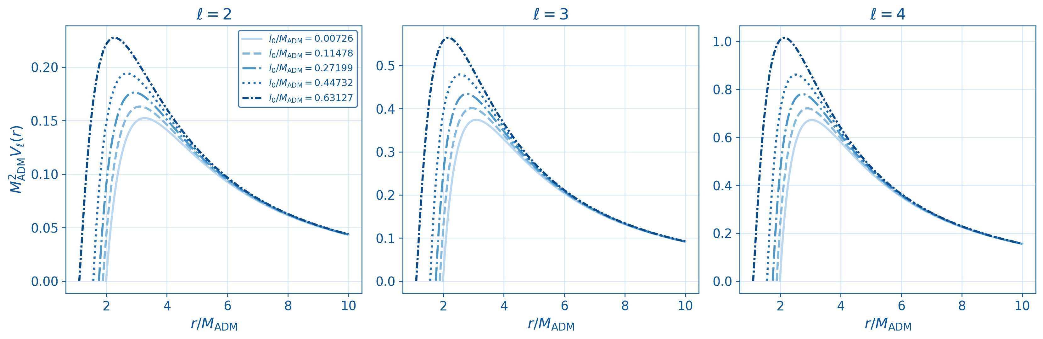
The dependence of the axial barrier on the zero-point length and on the multipole number is illustrated in Fig. 2. The potentials are plotted in ADM-scaled variables, $M_{\rm ADM}^{2}V_{\ell}$ versus $r/M_{\rm ADM}$, for representative values of $l_{0}$ used in the frequency tables. For fixed $\ell$, increasing $l_{0}/M_{\rm ADM}$ raises the height of the barrier and shifts its maximum toward smaller $r/M_{\rm ADM}$. At fixed $l_{0}/M_{\rm ADM}$, larger multipoles produce the expected higher and narrower Regge–Wheeler barrier. The largest displayed value is the near-extremal case $l_{0}=0.85$, corresponding to $l_{0}/M_{\rm ADM}=0.63127$ for $M=1$.

The numerical analysis combines a frequency-domain calculation with a direct evolution of the master equation. The tabulated spectra are obtained from a high-order WKB expansion improved by Padé resummation. This approach is particularly efficient for the axial gravitational potential considered here, because the potential has the usual single-barrier shape illustrated in Fig. 2. The time-domain calculation is used as a separate diagnostic: it evolves the same wave equation without expanding around the potential maximum and then extracts the dominant ringing frequency from the waveform.

The tables in this section list the WKB–Padé frequencies in units of the parameter $M$, which was set equal to unity in the numerical integration. Since the physical asymptotic mass of the self-energy geometry is instead $M_{\rm ADM}=1+3\pi/(32l_{0})$, it is also useful to present the same spectra in ADM units. In Figs. 3 and 4 we therefore plot $M_{\rm ADM}\omega$ as a function of the dimensionless ratio $l_{0}/M_{\rm ADM}$. This rescaling removes the large change of the total mass at small $l_{0}$ and makes the deformation of the spectrum by the zero-point length more transparent.

For the fundamental modes shown in Fig. 3, the oscillation frequency grows monotonically with $l_{0}/M_{\rm ADM}$ for all three multipoles up to the near-extremal point $l_{0}=0.85$. The damping rate $-\mathrm{Im}(M_{\rm ADM}\omega)$ behaves differently: it has a shallow maximum near $l_{0}=0.35$ and then decreases increasingly rapidly toward the near-extremal endpoint. Thus, in ADM units, the self-energy correction makes the fundamental gravitational modes oscillate faster, while the damping is reduced in the region closest to extremality. The hierarchy with respect to $\ell$ remains the expected one: larger $\ell$ gives a larger real part and a slightly larger damping rate.

This trend is consistent with the potential profiles in Fig. 2: in the WKB picture, the real part of the QNM frequency is controlled mainly by the barrier height $V_{0}$, so the higher barriers produced by larger $l_{0}/M_{\rm ADM}$ naturally lead to larger oscillation frequencies.

The damping rate is controlled by a different combination of barrier properties. At leading WKB order,

$$-{\rm Im}(\omega)\simeq\left(n+\frac{1}{2}\right)\frac{\sqrt{-2V_{0}^{(2)}}}{2\sqrt{V_{0}}},$$

(27)

where $V_{0}^{(2)}$ is the second derivative with respect to $r_{*}$ at the maximum. Although $V_{0}$ grows monotonically with $l_{0}/M_{\rm ADM}$, the curvature-to-height ratio in this expression first increases slightly and then decreases. As the two horizons approach degeneracy, the surface gravity decreases and the barrier becomes broader in the tortoise coordinate, reducing its normalized curvature. The competition between the increasing height and the subsequent broadening therefore explains why the fundamental oscillation frequency remains monotonic while its damping rate develops a maximum and then decreases.

The overtone data for $\ell=2$ are summarized in Fig. 4. After ADM rescaling, the real parts of the $n=1$ and $n=2$ modes increase monotonically up to $l_{0}=0.85$, whereas the $n=3$ real part reaches its largest tabulated value at $l_{0}=0.80$ and turns over at $l_{0}=0.85$. The damping rates remain ordered by overtone number; they reach shallow maxima at small or intermediate $l_{0}/M_{\rm ADM}$ and then decrease toward the near-extremal endpoint. The close agreement between the 16th- and 14th-order Padé values in the tables indicates that these trends are not artifacts of the WKB order.

The turnover of the $n=3$ real part is likewise associated with the near-extremal change in the barrier shape rather than with its height alone. Higher overtones depend more strongly on the higher derivatives entering the WKB corrections and probe a wider portion of the potential, including the increasingly stretched near-horizon region. Near $l_{0}=0.85$, these shape corrections become large enough to overcome the upward shift produced by the increasing peak height. The effect is unlikely to be a WKB truncation artifact: the ADM-scaled $n=3$ real part decreases by about $2.5\%$ between $l_{0}=0.80$ and $0.85$, whereas the difference between the two Padé orders at $l_{0}=0.85$ is about $0.16\%$. The potential remains a smooth single barrier and all imaginary parts remain negative, so this behavior does not indicate an instability; nevertheless, an independent continued-fraction calculation would be a useful quantitative check.

For completeness, the numerical values used to construct these plots are displayed in Tables I and II in the original $M=1$ normalization. The last column gives the relative difference between the two Padé-resummed WKB orders and provides a compact estimate of the numerical stability.

The time-domain signals in Figs. 5 and 6 provide independent checks of both the ringdown frequencies and the asymptotic decay. For $\ell=2$ and $l_{0}=0.65$, the WKB–Padé value is $\omega_{\rm WKB}=0.294347-0.060148i$, while the Prony extraction gives $\omega_{\rm TD}=0.29435-0.06015i$. For $\ell=3$ and $l_{0}=0.8$, the corresponding values are $\omega_{\rm WKB}=0.529374-0.061803i$ and $\omega_{\rm TD}=0.5294-0.0618i$. Using the complex relative difference

$$\Delta_{\rm TD/WKB}=\frac{|\omega_{\rm TD}-\omega_{\rm WKB}|}{|\omega_{\rm WKB}|}\times 100\%,$$

(28)

one obtains $\Delta_{\rm TD/WKB}=1.20\times 10^{-3}\%$ for the $\ell=2$ profile and $4.91\times 10^{-3}\%$ for the $\ell=3$ profile. The corresponding relative differences between the damping rates are $3.33\times 10^{-3}\%$ and $4.85\times 10^{-3}\%$, respectively. This agreement is consistent with the expected accuracy of the comparison: the WKB–Padé values are very stable for the fundamental modes, whereas the time-domain estimates are limited mainly by the choice of the Prony fitting window, residual contamination from the prompt response, and the onset of the late-time tail.

At later times, the logarithmic plot in Fig. 5 (b) displays a straight asymptotic segment proportional to $t^{-7}$. This is exactly the Price-law exponent $t^{-(2\ell+3)}$ for a massless perturbation with compact initial data at fixed radius when $\ell=2$ Price (1972). A similar result for $\ell=3$ and $l_{0}=0.8$ is shown in Fig. 6. The result is physically expected in the present geometry because the spacetime is asymptotically flat and the axial gravitational potential has the same leading centrifugal term and the same long-range $1/r^{3}$ structure that controls the Schwarzschild tail, while the zero-point-length corrections enter only through subleading inverse powers of $r$. Therefore, the numerical evolution confirms that the self-energy regularization changes the quasinormal ringing frequencies but does not alter the leading quadrupole Price-law tail in the asymptotic regime shown here.