Power Convexity of Solutions to the Complex Monge-Ampère Equation $\det(u_{{i\overline{j}}})=1$ in Complex Dimension Two

Hongyu Chen Jingchen Hu Li Sheng

Abstract

In this paper, we establish the power convexity of solutions to the complex Monge-Ampère equation $\det(u_{{i\overline{j}}})=1$ in a convex set in the complex 2 dimensional Euclidean space. Even the convexity result is only for 2 dimension, our approach is applicable to all dimensions.

1 Introduction

Convexity properties of solutions are a classical and fundamental theme in elliptic partial differential equations. It is interesting to investigate if the solution $u$ of a partial differential equation is convex, and, if not, can you find a suitable monotone function $g(t)$ so that $g(u)$ is convex.

This line of inquiry was profoundly advanced by the pivotal work of [CF85], who established the strict power convexity of solutions for a class of semilinear elliptic equations in real dimension two

\begin{cases}\Delta u=f(u)&\text{ in }\Omega,\\ u=M&\text{ on }\partial\Omega,\end{cases}

(1.1)

where $\Omega$ is a bounded convex domain in $\mathbb{R}^{2}$ and $M$ is a real constant. Since then, this technique has been extensively studied and generalized by many authors, such as [MX08], [BG09], [BGMX11], [GX13], [SW16], and [CJX25].

Also, very recently, works of Chen-Ma-Li-Salani established the power convexity of solutions to real $\sigma_{2}$ Hessian equation [LMS26] and the logarithmic convexity of solutions to complex $\sigma_{2}$ Hessian eigenvalue problem [CLM26].

In this paper, we investigate the power convexity of solutions to the Dirichlet problem for the complex Monge-Ampère equation. Specifically, let $\Omega$ be a strictly convex bounded domain in $\mathbb{C}^{n}$ , and let $u:\overline{\Omega}\rightarrow\mathbb{R}$ be the solution of the following Dirichelt problem:

Problem 1.

\begin{cases}\det\left(u_{i\bar{j}}\right)=1&\text{in\ }\Omega,\\ u=0&\text{on }\partial\Omega.\end{cases}

(1.2)

It is known that the solution $u$ itself is in general not convex in $\Omega$ . This leads naturally to the question of whether, for a given exponent $0<\alpha<1$ , the power function $-(-u)^{\alpha}$ is convex in $\Omega$ . In this paper, we establish the convexity of $-\sqrt{-u}$ in the case of complex dimension $2$ .

Theorem 1.1.

Let $\Omega$ be a strictly convex bounded domain in $\mathbb{C}^{2}$ with smooth boundary and $u\in C^{4}(\Omega)\cap C^{2}(\overline{\Omega})$ be the classical solution of (1.2). Then $-\sqrt{-u}$ is strictly convex in $\Omega$ .

This result is also proved by a very recent paper of Zhang-Zhou [ZZ26], using a different method.

In this paper, we employ a method developed in [H25], [H24B], [H24A] and [HS26], which could be used to study the real convexity(positivity of the real Hessian) of a solution using complex derivatives. Specifically, in this paper, we introduce a real-valued auxiliary function $\sigma$ ( involving only complex derivatives $u_{{i\overline{j}}},\ u_{ij},u_{i}$ , where $i,j$ are indices for complex coordinates) quantifying the convexity of $-\sqrt{-u}$ , so that proving the strict convexity of $-\sqrt{-u}$ is reduced to proving the positivity of $\sigma$ . The advantage is that for an equation involving only complex derivatives $u_{{i\overline{j}}}$ , using complex derivatives of $u$ is much easier than using real derivatives of $u$ .

The paper is organized as follows. In Section 2, we derive differential equations for the second derivatives of the solution $u$ and $-\sqrt{-u}$ . In Section 3, we estimate the minimal eigenvalue of $\mathcal{M}\mathcal{A}^{-1}$ . Section 3.1 and 3.2 treat the case where the minimal eigenvalue of $\mathcal{M}\mathcal{A}^{-1}$ is strictly smaller than the second minimal eigenvalue of $\mathcal{M}\mathcal{A}^{-1}$ , while Section 3.3 addresses the general case via approximation.

2 Differential Equations for Second Derivatives and Their Modifications

Suppose that $u$ is a solution to equation (1.2). In this section, we derive the important equations satisfied by the second derivatives of $u$ and $v:=-\sqrt{-u}$ .

2.1 Equations for Second Derivatives of $u$

We apply $\partial_{i}$ to the equation of $u$ :

\log\left[\det(u_{p\bar{q}})\right]=\text{constant },

and get

u^{\bar{q}p}u_{p\bar{q}i}=0.

(2.1)

Remark 1.

Throughout this paper, we adopt the convention that the first index of a matrix entry is the row index and the second index is the column index. For instance, we write the inverse of invertible $A$ as

A^{-1}=(A^{\bar{j}i}),

(2.2)

meaning that $j$ is the row index and $i$ is the column index (equivalently, $A_{k\bar{j}}\,A^{\bar{j}i}=\delta_{k}^{\,i}$ ). For the inverse of the complex conjugate matrix $\overline{A}$ , we write

\overline{A}^{-1}=(A^{j\bar{i}}),

(2.3)

where $j$ is the row index and $i$ is the column index; in particular, $A^{j\bar{i}}=\overline{A^{\bar{j}i}}$ . Moreover, if $A$ is Hermitian, then its inverse is also Hermitian. In particular, at the level of entries we have $A^{\bar{j}i}=A^{i\bar{j}}$

Then we apply $\partial_{\bar{j}}$ to equation (2.1) and get

u^{\bar{q}p}u_{p\bar{q}i\bar{j}}-u^{\bar{q}s}u_{s\bar{t}\bar{j}}u^{\bar{t}p}u_{p\bar{q}i}=0.

(2.4)

We switch indices $p$ and $s$ in the second term of equation (2.4) and get

u^{\bar{q}p}u_{p\bar{q}i\bar{j}}-u^{\bar{q}p}u_{p\bar{t}\bar{j}}u^{\bar{t}s}u_{s\bar{q}i}=0.

(2.5)

We switch indices $t$ and $q$ in the second term of equation (2.4) and get

u^{\bar{q}p}u_{p\bar{q}i\bar{j}}-u^{\bar{t}s}u_{s\bar{q}\bar{j}}u^{\bar{q}p}u_{p\bar{t}i}=0.

(2.6)

Let

A=(A_{i\bar{j}})=(u_{i\bar{j}}),\quad B=(B_{ij})=(u_{ij}),

where $i$ is the row index and $j$ is the column index.

Since $u$ is strictly plurisubharmonic, the Hermitian matrix $A$ is positive definite. It is convenient to write equations (2.5) and (2.6) as equations for matrices. Here, let $i$ be the row index and $j$ be the column index in equations (2.5) and (2.6). Then equation (2.5) becomes

u^{\bar{q}p}\partial_{p\bar{q}}A=u^{\bar{q}p}\partial_{\bar{q}}B\overline{A}^{-1}\partial_{p}\overline{B},

(2.7)

and equation (2.6) becomes

u^{\bar{q}p}\partial_{p\bar{q}}A=u^{\bar{q}p}\partial_{p}AA^{-1}\partial_{\bar{q}}A.

(2.8)

Similarly, we apply $\partial_{j}$ to equation (2.1) and get

u^{\bar{q}p}u_{p\bar{q}ij}-u^{\bar{q}s}u_{s\bar{t}j}u^{\bar{t}p}u_{p\bar{q}i}=0.

(2.9)

We switch indices $p$ and $s$ in the second term of equation (2.9) and get

u^{\bar{q}p}u_{p\bar{q}ij}-u^{\bar{q}p}u_{p\bar{t}j}u^{\bar{t}s}u_{s\bar{q}i}=0.

(2.10)

We switch indices $q$ and $t$ in the second term of equation (2.9) and get

u^{\bar{q}p}u_{p\bar{q}ij}-u^{\bar{t}s}u_{s\bar{q}j}u^{\bar{q}p}u_{p\bar{t}i}=0.

(2.11)

We express equations (2.10) and (2.11) as matrices, where $i$ and $j$ denote the row and column indices, respectively. Then equation (2.10) becomes

u^{\bar{q}p}\partial_{p\bar{q}}B=u^{\bar{q}p}\partial_{\bar{q}}B\overline{A}^{-1}\partial_{p}\overline{A},

(2.12)

and equation (2.11) becomes

u^{\bar{q}p}\partial_{p\bar{q}}B=u^{\bar{q}p}\partial_{p}AA^{-1}\partial_{\bar{q}}B.

(2.13)

Notice that equations (2.8), (2.7), (2.12) and (2.13) are analogs of equations (2.2) (2.3) of [H25]. The following equations are equivalent to equations (2.12) and (2.13), and they are very useful for subsequent computations. Equation

u^{\bar{q}p}\partial_{p}\left(\partial_{\bar{q}}B\overline{A}^{-1}\right)=0

(2.14)

is equivalent to equation (2.12). Equation

u^{\bar{q}p}\partial_{\bar{q}}\left(\overline{A}^{-1}\partial_{p}\overline{B}\right)=0

(2.15)

is equivalent to the conjugate of equation (2.12). Then we apply $u^{\bar{q}p}\partial_{p\bar{q}}$ to the matrix

M=A-B\overline{A}^{-1}\overline{B}

(2.16)

and get

u^{\bar{q}p}\partial_{p\bar{q}}M=u^{\bar{q}p}\partial_{\bar{q}}\left(\partial_{p}A-\mathbb{B}^{(p)}\overline{A}^{-1}\overline{B}-B\overline{A}^{-1}\partial_{p}\overline{B}\right).

(2.17)

In the above, for the sake of simplifying the following computation, we introduce a new matrix

\mathbb{B}^{(p)}=\partial_{p}B-B\overline{A}^{-1}\partial_{p}\overline{A},

(2.18)

such that

\mathbb{B}^{(p)}\overline{A}^{-1}=\partial_{p}\left(B\overline{A}^{-1}\right).

(2.19)

Taking the conjugate transpose of equation (2.19) yields

\overline{A}^{-1}\left(\mathbb{B}^{(q)}\right)^{*}=\partial_{\bar{q}}\left(\overline{A}^{-1}\overline{B}\right).

(2.20)

Then

	$\displaystyle u^{\bar{q}p}\partial_{p\bar{q}}M$	$\displaystyle=u^{\bar{q}p}\left(\partial_{p\bar{q}}A-\partial_{\bar{q}}B\overline{A}^{-1}\partial_{p}\overline{B}\right)-u^{\bar{q}p}B\partial_{\bar{q}}\left(\overline{A}^{-1}\partial_{p}\overline{B}\right)$
		$\displaystyle\hskip 8.61108pt+u^{\bar{q}p}\left[-\partial_{\bar{q}}\mathbb{B}^{(p)}\overline{A}^{-1}\overline{B}-\mathbb{B}^{(p)}\overline{A}^{-1}\left(\mathbb{B}^{(q)}\right)^{*}\right]$		(2.21)

Using (2.7) and (2.15), the equation above can be simplified:

\displaystyle u^{\bar{q}p}\partial_{p\bar{q}}M=-u^{\bar{q}p}\partial_{\bar{q}}\mathbb{B}^{(p)}\overline{A}^{-1}\overline{B}-u^{\bar{q}p}\mathbb{B}^{(p)}\overline{A}^{-1}\left(\mathbb{B}^{(q)}\right)^{*}.

(2.22)

We need to compute $u^{\bar{q}p}\partial_{\bar{q}}\mathbb{B}^{(p)}$ in (2.22). Applying $u^{\bar{q}p}\partial_{\bar{q}}$ directly to equation (2.18) yields

	$\displaystyle u^{\bar{q}p}\partial_{\bar{q}}\mathbb{B}^{(p)}$	$\displaystyle=u^{\bar{q}p}\left(\partial_{p\bar{q}}B-\partial_{\bar{q}}B\overline{A}^{-1}\partial_{p}\overline{A}+B\overline{A}^{-1}\partial_{\bar{q}}\overline{A}\overline{A}^{-1}\partial_{p}\overline{A}-B\overline{A}^{-1}\partial_{p\bar{q}}\overline{A}\right)$
		$\displaystyle=u^{\bar{q}p}\left[\left(\partial_{p\bar{q}}B-\partial_{\bar{q}}B\overline{A}^{-1}\partial_{p}\overline{A}\right)-B\overline{A}^{-1}\left(\partial_{\bar{q}}\overline{A}\overline{A}^{-1}\partial_{p}\overline{A}-\partial_{p\bar{q}}\overline{A}\right)\right].$

Using equations (2.12) and (2.8), we obtain $u^{\bar{q}p}\partial_{\bar{q}}\mathbb{B}^{(p)}=0$ . So we find

u^{\bar{q}p}\partial_{p\bar{q}}M=-u^{\bar{q}p}\mathbb{B}^{(p)}\overline{A}^{-1}\left(\mathbb{B}^{(q)}\right)^{*}\leq 0.

(2.23)

Here, for an $n\times n$ matrix $M$ , we write

M<C\quad(\text{ or }\,M>C),

(2.24)

if all eigenvalues of $M$ are real and $<C$ ( or $>C$ ); similarly we denote $M\leq C$ or $M\geq C$ when equalities are included.

This inequality (2.23) implies if $M\geq 0$ (positive definite) on $\partial\Omega$ , then $M>0$ in $\Omega$ . By Lemma A.6 of [H25] or Lemma A.1 of this paper, the strict convexity of $u$ is equivalent to the conditions $A>0$ and $M>0$ . So the inequality (2.23) implies that if u is strictly convex on $\partial\Omega$ , then it is strictly convex in $\Omega$ .

However, there are many examples showing $u$ may not be convex on $\partial\Omega$ , even $\Omega$ is a strictly convex domain. So we turn to prove the convexity of a funtion of $u$ , in particular, we study the convexity of $v:=-\sqrt{-u}$ .

2.2 Differential Equations of Second Derivatives of $v$

By the maximum principle and the boundary condition $u(x)=0$ for $x\in\partial\Omega$ , we conclude that $-u>0$ in $\Omega$ . The Hessian matrices of $v:=-\sqrt{-u}$ are given by

\displaystyle v_{i\bar{j}}=\frac{1}{2(-u)^{\frac{1}{2}}}\left[u_{i\bar{j}}+\frac{u_{i}u_{\bar{j}}}{-2u}\right],\ v_{ij}=\frac{1}{2(-u)^{\frac{1}{2}}}\left[u_{ij}+\frac{u_{i}u_{j}}{-2u}\right].

(2.25)

Let

\mathcal{A}=(\mathcal{A}_{i\bar{j}})=\left(u_{i\bar{j}}+\frac{u_{i}u_{\bar{j}}}{-2u}\right),\quad\mathcal{B}=(\mathcal{B}_{ij})=\left(u_{ij}+\frac{u_{i}u_{j}}{-2u}\right),

(2.26)

where $i$ is the row index and $j$ is the column index. Then the matrix $\mathcal{A}$ is positive definite. Let

\mathcal{M}=\mathcal{A}-\mathcal{B}\overline{\mathcal{A}}^{-1}\overline{\mathcal{B}}.

(2.27)

By Lemma A.6 of [H25] or Lemma A.1 of this paper, the convexity of $v$ is equivalent to the positive definiteness of both $\mathcal{A}$ and $\mathcal{M}$ .

Let

\Omega_{\delta}=\{x\in\Omega\;|\;\text{dist}(x,\partial\Omega)>\delta\}.

(2.28)

According to the $C^{2}$ estimate for Problem 1, the minimum eigenvalue of $(u_{{i\overline{j}}})$ has a positive lower bound estimate in $\Omega$ , depending on the convexity and regularity of $\Omega$ . Since $\mathcal{A}>A=(u_{{i\overline{j}}})$ , the minimum eigenvalue of $\mathcal{A}$ also has a positive lower bound in $\Omega$ . If $\Omega$ is smooth and strictly convex, then it’s well known that $v$ is strictly convex in $\Omega_{\delta}\setminus\Omega_{2\delta}$ when $\delta$ is small enough. Hence, $\mathcal{M}>0$ in $\Omega_{\delta}\setminus\Omega_{2\delta}$ . We need to show that this is also true in $\Omega_{2\delta}$ . To do this, let

\displaystyle\mathcal{K}=\mathcal{M}\mathcal{A}^{-1},

(2.29)

and we aim to prove that the minimum eigenvalue of $\mathcal{K}>0$ . We compute and find

\displaystyle u^{\bar{q}p}(\lambda_{\min}\mathcal{K})_{p\bar{q}}\leq C(\lambda_{\min}\mathcal{K}+|\nabla\lambda_{\min}\mathcal{K}|),

(2.30)

when the minimum eigenvalue of $\mathcal{K}$ is different from the second minimal eigenvalue of $\mathcal{K}$ in section 3 in the case of complex dimension 2. Then we can use this to derive a positive lower bound for the minimum eigenvalue of $\mathcal{K}$ .

In this section, we derive the differential relations for $\mathcal{A}$ and $\mathcal{B}$ , analogous to the relations (2.7), (2.8), (2.13) and (2.12).

In the computation for $u^{\bar{q}p}\partial_{p\bar{q}}M\leq 0$ , we used the following relations

•

$u^{\bar{q}p}\left(\partial_{p\bar{q}}A-\partial_{\bar{q}}B\overline{A}^{-1}\partial_{p}\overline{B}\right)=0$ ,
•

$u^{\bar{q}p}\left(\partial_{p\bar{q}}\overline{A}-\partial_{\bar{q}}\overline{A}\overline{A}^{-1}\partial_{p}\overline{A}\right)=0$ ,
•

$u^{\bar{q}p}\left(\partial_{p\bar{q}}B-\partial_{\bar{q}}B\overline{A}^{-1}\partial_{p}\overline{A}\right)=0$ ,
•

$u^{\bar{q}p}\left(\partial_{p\bar{q}}\overline{B}-\partial_{\bar{q}}\overline{A}\overline{A}^{-1}\partial_{p}\overline{B}\right)=0$ .

When we compute $u^{\bar{q}p}(\lambda_{\min}\mathcal{K})$ , we find it’s deeply related to computing

\displaystyle u^{\bar{q}p}\partial_{p\bar{q}}\mathcal{M}.

(2.31)

In the computation of $u^{\bar{q}p}\partial_{p\bar{q}}\mathcal{M}$ , the four relations above still appear but with some modifications. To simplify the computation, we introduce

\mathscr{B}^{(p)}=\partial_{p}\mathcal{B}-\mathcal{B}\overline{\mathcal{A}}^{-1}\partial_{p}\overline{\mathcal{A}}.

(2.32)

With this notation, we have

\mathscr{B}^{(p)}\overline{\mathcal{A}}^{-1}=\partial_{p}\left(\mathcal{B}\overline{\mathcal{A}}^{-1}\right).

(2.33)

Taking the conjugate transpose of equation (2.33) yields

\overline{\mathcal{A}}^{-1}(\mathscr{B}^{(q)})^{*}=\partial_{\bar{q}}(\overline{\mathcal{A}}^{-1}\overline{\mathcal{B}}).

(2.34)

First we compute $\partial_{p}\mathcal{M}$ :

\displaystyle\partial_{p}\mathcal{M}=\partial_{p}\mathcal{A}-\mathscr{B}^{(p)}{\overline{\mathcal{A}}}^{-1}\overline{\mathcal{B}}-\mathcal{B}{\overline{\mathcal{A}}}^{-1}\partial_{p}{\overline{\mathcal{B}}}.

(2.35)

Then we apply $\partial_{\overline{q}}$ to the equation above. Simply using Leibniz rule, we get

		$\displaystyle u^{\bar{q}p}\partial_{p\bar{q}}\mathcal{M}=u^{\bar{q}p}\left(\partial_{p\bar{q}}\mathcal{A}-\partial_{\bar{q}}\mathcal{B}\overline{\mathcal{A}}^{-1}\partial_{p}\overline{\mathcal{B}}\right)-u^{\bar{q}p}\mathcal{B}\partial_{\bar{q}}\left(\overline{\mathcal{A}}^{-1}\partial_{p}\overline{\mathcal{B}}\right)$
		$\displaystyle\hskip 8.61108pt+u^{\bar{q}p}\left[-\partial_{\bar{q}}\mathscr{B}^{(p)}\overline{\mathcal{A}}^{-1}\overline{\mathcal{B}}-\mathscr{B}^{(p)}\overline{\mathcal{A}}^{-1}\left(\partial_{q}\mathscr{B}\right)^{*}\right],$		(2.36)

which is very similar to (2.21). In above

\displaystyle\partial_{\overline{q}}\left(\overline{\mathcal{A}}^{-1}\partial_{p}\overline{\mathcal{B}}\right)=-{\overline{\mathcal{A}}}^{-1}\left(\partial_{{\overline{q}}}{\overline{\mathcal{A}}}{\overline{\mathcal{A}}}^{-1}\partial_{p}\overline{\mathcal{B}}-\partial_{{p\overline{q}}}{\overline{\mathcal{B}}}\right)

(2.37)

and

	$\displaystyle\partial_{\bar{q}}\mathscr{B}^{(p)}$	$\displaystyle=\partial_{{\overline{q}}}\left(\partial_{p}\mathcal{B}-\mathcal{B}{\overline{\mathcal{A}}}^{-1}\partial_{p}{\overline{\mathcal{A}}}\right)$
	$\displaystyle=$	$\displaystyle\left(\partial_{p\overline{q}}\mathcal{B}-\partial_{\overline{q}}\mathcal{B}{\overline{\mathcal{A}}}^{-1}\partial_{p}{\overline{\mathcal{A}}}^{-1}\right)-\mathcal{B}{\overline{\mathcal{A}}}^{-1}\left(\partial_{p\bar{q}}\overline{\mathcal{A}}-\partial_{\bar{q}}\overline{\mathcal{A}}\overline{\mathcal{A}}^{-1}\partial_{p}\overline{\mathcal{A}}\right).$		(2.38)

Plugging (2.37) and (2.2) into (2.36), we get

		$\displaystyle\ \ u^{\bar{q}p}\partial_{p\bar{q}}\mathcal{M}$
		$\displaystyle=u^{\bar{q}p}\left(\partial_{p\bar{q}}\mathcal{A}-\partial_{\bar{q}}\mathcal{B}\overline{\mathcal{A}}^{-1}\partial_{p}\overline{\mathcal{B}}\right)+\mathcal{B}\overline{\mathcal{A}}^{-1}u^{\bar{q}p}\left(\partial_{p\bar{q}}\overline{\mathcal{A}}-\partial_{\bar{q}}\overline{\mathcal{A}}\overline{\mathcal{A}}^{-1}\partial_{p}\overline{\mathcal{A}}\right)\overline{\mathcal{A}}^{-1}\overline{\mathcal{B}}$
		$\displaystyle\hskip 8.61108pt-u^{\bar{q}p}\left(\partial_{p\bar{q}}\mathcal{B}-\partial_{\bar{q}}\mathcal{B}\overline{\mathcal{A}}^{-1}\partial_{p}\overline{\mathcal{A}}\right)\overline{\mathcal{A}}^{-1}\overline{\mathcal{B}}-\mathcal{B}\overline{\mathcal{A}}^{-1}u^{\bar{q}p}\left(\partial_{p\bar{q}}\overline{\mathcal{B}}-\partial_{\bar{q}}\overline{\mathcal{A}}\overline{\mathcal{A}}^{-1}\partial_{p}\overline{\mathcal{B}}\right)$
		$\displaystyle\hskip 8.61108pt-u^{\bar{q}p}\mathscr{B}^{(p)}\overline{\mathcal{A}}^{-1}\left(\mathscr{B}^{(q)}\right)^{*}.$		(2.39)

Similar to the computation for $u^{\bar{q}p}\partial_{p\bar{q}}M$ , evaluating (2.39) requires to compute the following relations:

•

$u^{\bar{q}p}\left(\partial_{p\bar{q}}\mathcal{A}-\partial_{\bar{q}}\mathcal{B}\overline{\mathcal{A}}^{-1}\partial_{p}\overline{\mathcal{B}}\right)$ ,
•

$u^{\bar{q}p}\left(\partial_{p\bar{q}}\overline{\mathcal{A}}-\partial_{\overline{q}}\overline{\mathcal{A}}\overline{\mathcal{A}}^{-1}\partial_{p}\overline{\mathcal{A}}\right)$ ,
•

$u^{\bar{q}p}\left(\partial_{p\bar{q}}\mathcal{B}-\partial_{\bar{q}}\mathcal{B}\overline{\mathcal{A}}^{-1}\partial_{p}\overline{\mathcal{A}}\right)$ ,
•

$u^{\bar{q}p}\left(\partial_{p\bar{q}}\overline{\mathcal{B}}-\partial_{\bar{q}}\overline{\mathcal{A}}\overline{\mathcal{A}}^{-1}\partial_{p}\overline{\mathcal{B}}\right)$ .

We first compute the derivatives of $\mathcal{A}$ and $\mathcal{B}$ . It is convenient to define $h(u)=\frac{1}{-2u}$ , whose derivative is $h^{\prime}=2h^{2}$ . By direct computation, we get

	$\displaystyle\partial_{p}\mathcal{A}_{i\bar{j}}$	$\displaystyle=\partial_{p}A_{i\bar{j}}+u_{ip}u_{\bar{j}}h+u_{i}u_{p\bar{j}}h+u_{i}u_{\bar{j}}u_{p}h^{\prime}$
		$\displaystyle=\partial_{p}A_{i\bar{j}}+hu_{\bar{j}}\mathcal{B}_{ip}+hu_{i}\mathcal{A}_{p\bar{j}}.$		(2.40)

Similarly, we have

$\displaystyle\partial_{\bar{q}}\mathcal{A}_{i\bar{j}}$	$\displaystyle=\partial_{\bar{q}}A_{i\bar{j}}+hu_{\bar{j}}\mathcal{A}_{i\bar{q}}+hu_{i}\overline{\mathcal{B}_{qj}},$	(2.41)
$\displaystyle\partial_{p}\mathcal{B}_{ij}$	$\displaystyle=\partial_{p}B_{ij}+hu_{j}\mathcal{B}_{ip}+hu_{i}\mathcal{B}_{pj},$	(2.42)
$\displaystyle\partial_{\bar{q}}\mathcal{B}_{ij}$	$\displaystyle=\partial_{\bar{q}}B_{ij}+hu_{j}\mathcal{A}_{i\bar{q}}+hu_{i}\mathcal{A}_{j\bar{q}},$	(2.43)
$\displaystyle\partial_{p}\mathcal{B}_{\bar{i}\bar{j}}$	$\displaystyle=\partial_{p}B_{\bar{i}\bar{j}}+hu_{\bar{j}}\mathcal{A}_{p\bar{i}}+hu_{\bar{i}}\mathcal{A}_{p\bar{j}}.$	(2.44)

We plug these into

\partial_{p}\mathcal{M}=\partial_{p}\mathcal{A}-\mathscr{B}^{(p)}\overline{\mathcal{A}}^{-1}\overline{\mathcal{B}}-\mathcal{B}\overline{\mathcal{A}}^{-1}\partial_{p}\overline{\mathcal{B}}.

(2.45)

In the case that $\mathcal{A}=I$ and $\mathcal{B}=\mathrm{diag}(b_{1},\cdots,b_{n})$ , for $b_{k}\in\mathbb{R}^{\geq 0}$ , we get

		$\displaystyle\hskip 8.61108pt\partial_{p}\mathcal{M}_{i\bar{j}}$
		$\displaystyle=u_{i\bar{j}p}+hu_{\bar{j}}\mathcal{B}_{ip}+hu_{i}\mathcal{A}_{p\bar{j}}-b_{j}\mathscr{B}^{(p)}_{i{j}}-b_{i}u_{\bar{i}\bar{j}p}-hb_{i}u_{\bar{j}}\mathcal{A}_{p\bar{i}}-hb_{i}u_{\bar{i}}\mathcal{A}_{p\bar{j}}$
		$\displaystyle=u_{i\bar{j}p}-b_{i}u_{\bar{i}\bar{j}p}+hu_{i}\delta_{jp}-hb_{i}u_{\bar{i}}\delta_{jp}-b_{j}\mathscr{B}^{(p)}_{i{j}}.$		(2.46)

When $i=j=1$ , we get

\partial_{p}\mathcal{M}_{1\bar{1}}=u_{1\bar{1}p}-b_{1}u_{\bar{1}\bar{1}p}+hu_{1}\delta_{1p}-hb_{1}u_{\bar{1}}\delta_{1p}-b_{1}\mathscr{B}^{(p)}_{11}.

(2.47)

Then we compute the second derivatives of $\mathcal{A}_{i\bar{j}}$

	$\displaystyle\partial_{p\bar{q}}\mathcal{A}_{i\bar{j}}$	$\displaystyle=\partial_{p\bar{q}}A_{i\bar{j}}+h^{\prime}u_{\bar{q}}u_{\bar{j}}\mathcal{B}_{ip}+hu_{\bar{j}\bar{q}}\mathcal{B}_{ip}+hu_{\bar{j}}\partial_{\bar{q}}\mathcal{B}_{ip}$
		$\displaystyle\hskip 8.61108pt+h^{\prime}u_{\bar{q}}u_{i}\mathcal{A}_{p\bar{j}}+hu_{i\bar{q}}\mathcal{A}_{p\bar{j}}+hu_{i}\partial_{\bar{q}}\mathcal{A}_{p\bar{j}}.$		(2.48)

We use $h^{\prime}=2h^{2}$ , $u_{\bar{j}\bar{q}}+hu_{\bar{j}}u_{\bar{q}}=\overline{\mathcal{B}_{jq}}$ and $u_{i\bar{q}}+hu_{i}u_{\bar{q}}=\mathcal{A}_{i\bar{q}}$ , and get

		$\displaystyle\partial_{p\bar{q}}\mathcal{A}_{i\bar{j}}=\partial_{p\bar{q}}A_{i\bar{j}}+hu_{\bar{j}}\partial_{\bar{q}}B_{ip}+hu_{i}\partial_{\bar{q}}A_{p\bar{j}}+h\mathcal{B}_{ip}\overline{\mathcal{B}_{jq}}+h\mathcal{A}_{i\bar{q}}\mathcal{A}_{p\bar{j}}$
		$\displaystyle+h^{2}u_{p}u_{\bar{j}}\mathcal{A}_{i\bar{q}}+2h^{2}u_{i}u_{\bar{j}}\mathcal{A}_{p\bar{q}}+h^{2}u_{i}u_{p}\overline{\mathcal{B}_{qj}}+h^{2}u_{\bar{j}}u_{\bar{q}}\mathcal{B}_{ip}+h^{2}u_{i}u_{\bar{q}}\mathcal{A}_{p\bar{j}}.$		(2.49)

As an analog of (2.7), we need to compute

u^{\bar{q}p}\partial_{p\bar{q}}\mathcal{A}-u^{\bar{q}p}\partial_{\bar{q}}\mathcal{B}\overline{\mathcal{A}}^{-1}\partial_{p}\overline{\mathcal{B}}

(2.50)

since it appears in (2.39). When computing $u^{\bar{q}p}\partial_{p\bar{q}}\mathcal{A}$ , we notice that on the right-hand side of (2.49)

\displaystyle u^{{p\overline{q}}}(hu_{\bar{j}}\partial_{\bar{q}}B_{ip}+hu_{i}\partial_{\bar{q}}A_{p\bar{j}})=0

(2.51)

since $u^{{p\overline{q}}}\partial_{\bar{q}}B_{ip}=u^{{p\overline{q}}}\partial_{\bar{q}}A_{p\bar{j}}=0$ . Then combining (2.49) and (2.43) yields

		$\displaystyle\left(u^{\bar{q}p}\partial_{p\bar{q}}\mathcal{A}-u^{\bar{q}p}\partial_{\bar{q}}\mathcal{B}\overline{\mathcal{A}}^{-1}\partial_{p}\overline{\mathcal{B}}\right)_{i\bar{j}}$
		$\displaystyle=u^{\bar{q}p}\partial_{p\bar{q}}\mathcal{A}_{i\bar{j}}-u^{\bar{q}p}(\partial_{\bar{q}}\mathcal{B})_{is}\mathcal{A}^{s\bar{t}}(\partial_{p}\overline{\mathcal{B}})_{\bar{t}\bar{j}}$
		$\displaystyle=u^{\bar{q}p}u_{is\bar{q}}(A^{s\bar{t}}-\mathcal{A}^{s\bar{t}})u_{\bar{j}\bar{t}p}+hu^{\bar{q}p}(\mathcal{B}_{ip}\mathcal{B}_{\bar{j}\bar{q}}+\mathcal{A}_{i\bar{q}}\mathcal{A}_{p\bar{j}})$
		$\displaystyle\hskip 8.61108pt-hu^{\bar{q}p}\mathcal{A}^{s\bar{t}}(u_{\bar{t}}u_{is\bar{q}}\mathcal{A}_{p\bar{j}}+u_{s}u_{\bar{j}\bar{t}p}\mathcal{A}_{i\bar{q}})$
		$\displaystyle\hskip 8.61108pt+h^{2}u^{\bar{q}p}(u_{i}u_{\bar{j}}\mathcal{A}_{p\bar{q}}+u_{i}u_{p}\mathcal{B}_{\bar{j}\bar{q}}+u_{\bar{j}}u_{\bar{q}}\mathcal{B}_{ip}-u_{s}u_{\bar{t}}\mathcal{A}^{s\bar{t}}\mathcal{A}_{i\bar{q}}\mathcal{A}_{p\bar{j}}).$		(2.52)

Similar to (2.8), we want to compute

u^{\bar{q}p}\partial_{p\bar{q}}\overline{\mathcal{A}}-u^{\bar{q}p}\partial_{\overline{q}}\overline{\mathcal{A}}\overline{\mathcal{A}}^{-1}\partial_{p}\overline{\mathcal{A}}.

(2.53)

Combining (2.49), (2.40) and (2.41) yields

		$\displaystyle\left(u^{\bar{q}p}\partial_{p\bar{q}}\overline{\mathcal{A}}-u^{\bar{q}p}\partial_{\overline{q}}\overline{\mathcal{A}}\overline{\mathcal{A}}^{-1}\partial_{p}\overline{\mathcal{A}}\right)_{\bar{i}j}$
		$\displaystyle=u^{\bar{q}p}\partial_{p\bar{q}}\overline{\mathcal{A}}_{\bar{i}j}-u^{\bar{q}p}(\partial_{\overline{q}}\overline{\mathcal{A}})_{\bar{i}s}\mathcal{A}^{s\bar{t}}(\partial_{p}\overline{\mathcal{A}})_{\bar{t}j}$
		$\displaystyle=u^{\bar{q}p}u_{s\bar{i}\bar{q}}(A^{s\bar{t}}-\mathcal{A}^{s\bar{t}})u_{j\bar{t}p}+hu^{\bar{q}p}(\mathcal{B}_{jp}\mathcal{B}_{\bar{i}\bar{q}}+\mathcal{A}_{j\bar{q}}\mathcal{A}_{p\bar{i}})$
		$\displaystyle\hskip 8.61108pt-hu^{\bar{q}p}\mathcal{A}^{s\bar{t}}(u_{\bar{t}}u_{s\bar{i}\bar{q}}\mathcal{B}_{jp}+u_{s}u_{j\bar{t}p}\mathcal{B}_{\bar{i}\bar{q}})$
		$\displaystyle\hskip 8.61108pt+h^{2}u^{\bar{q}p}(u_{j}u_{\bar{i}}\mathcal{A}_{p\bar{q}}+u_{p}u_{\bar{i}}\mathcal{A}_{j\bar{q}}+u_{j}u_{\bar{q}}\mathcal{A}_{p\bar{i}}-u_{s}u_{\bar{t}}\mathcal{A}^{s\bar{t}}\mathcal{B}_{jp}\mathcal{B}_{\bar{i}\bar{q}}).$		(2.54)

Also, we need to compute

u^{\bar{q}p}\partial_{p\bar{q}}\mathcal{B}-u^{\bar{q}p}\partial_{\bar{q}}\mathcal{B}\overline{\mathcal{A}}^{-1}\partial_{p}\overline{\mathcal{A}}.

(2.55)

Then, we compute the second derivatives of $\mathcal{B}_{ij}$

		$\displaystyle\partial_{p\bar{q}}\mathcal{B}_{ij}=\partial_{p}\left(\partial_{\bar{q}}B_{ij}+hu_{j}\mathcal{A}_{i\bar{q}}+hu_{i}\mathcal{A}_{j\bar{q}}\right)$
		$\displaystyle=\partial_{p\bar{q}}B_{ij}+hu_{j}\partial_{p}A_{i\bar{q}}+hu_{i}\partial_{p}A_{j\bar{q}}+h\mathcal{A}_{i\bar{q}}\mathcal{B}_{jp}+h\mathcal{A}_{j\bar{q}}\mathcal{B}_{ip}$
		$\displaystyle+h^{2}u_{p}u_{j}\mathcal{A}_{i\bar{q}}+h^{2}u_{i}u_{p}\mathcal{A}_{j\bar{q}}+2h^{2}u_{i}u_{j}\mathcal{A}_{p\bar{q}}+h^{2}u_{j}u_{\bar{q}}\mathcal{B}_{ip}+h^{2}u_{i}u_{\bar{q}}\mathcal{B}_{jp}.$		(2.56)

It follows that

		$\displaystyle\left(u^{\bar{q}p}\partial_{p\bar{q}}\mathcal{B}-u^{\bar{q}p}\partial_{\bar{q}}\mathcal{B}\overline{\mathcal{A}}^{-1}\partial_{p}\overline{\mathcal{A}}\right)_{ij}$
		$\displaystyle=u^{\bar{q}p}\partial_{p\bar{q}}\mathcal{B}_{ij}-u^{\bar{q}p}(\partial_{\bar{q}}\mathcal{B})_{is}\mathcal{A}^{s\bar{t}}(\partial_{p}\overline{\mathcal{A}})_{\bar{t}j}$
		$\displaystyle=u^{\bar{q}p}u_{is\bar{q}}(A^{s\bar{t}}-\mathcal{A}^{s\bar{t}})u_{j\bar{t}p}+hu^{\bar{q}p}(\mathcal{A}_{i\bar{q}}\mathcal{B}_{jp}+\mathcal{A}_{j\bar{q}}\mathcal{B}_{ip})$
		$\displaystyle\hskip 8.61108pt-hu^{\bar{q}p}\mathcal{A}^{s\bar{t}}(u_{\bar{t}}u_{is\bar{q}}\mathcal{B}_{pj}+u_{s}u_{j\bar{t}p}\mathcal{A}_{i\bar{q}})$
		$\displaystyle\hskip 8.61108pt+h^{2}u^{\bar{q}p}(u_{i}u_{j}\mathcal{A}_{p\bar{q}}+u_{i}u_{p}\mathcal{A}_{j\bar{q}}+u_{j}u_{\bar{q}}\mathcal{B}_{ip}-u_{s}u_{\bar{t}}\mathcal{A}^{s\bar{t}}\mathcal{A}_{i\bar{q}}\mathcal{B}_{jp}).$		(2.57)

It remains to compute the last term,

\partial_{p\bar{q}}\overline{\mathcal{B}}-\partial_{\bar{q}}\overline{\mathcal{A}}\overline{\mathcal{A}}^{-1}\partial_{p}\overline{\mathcal{B}}.

(2.58)

Then, we compute the second derivatives of $\mathcal{B}_{\bar{i}\bar{j}}$

		$\displaystyle\partial_{p\bar{q}}\mathcal{B}_{\bar{i}\bar{j}}=\partial_{p}(\partial_{\bar{q}}B_{\bar{i}\bar{j}}+hu_{\bar{i}}\mathcal{B}_{\bar{q}\bar{j}}+hu_{\bar{j}}\mathcal{B}_{\bar{q}\bar{i}})$
		$\displaystyle=\partial_{p\bar{q}}B_{\bar{i}\bar{j}}+hu_{\bar{i}}\partial_{p}B_{\bar{j}\bar{q}}+hu_{\bar{j}}\partial_{p}B_{\bar{i}\bar{q}}+h\mathcal{A}_{p\bar{i}}\mathcal{B}_{\bar{j}\bar{q}}+h\mathcal{A}_{p\bar{j}}\mathcal{B}_{\bar{q}\bar{i}}$
		$\displaystyle+h^{2}u_{p}u_{\bar{i}}\mathcal{B}_{\bar{j}\bar{q}}+h^{2}u_{p}u_{\bar{j}}\mathcal{B}_{\bar{i}\bar{q}}+2h^{2}u_{\bar{i}}u_{\bar{j}}\mathcal{A}_{p\bar{q}}+h^{2}u_{\bar{j}}u_{\bar{q}}\mathcal{A}_{p\bar{i}}+h^{2}u_{\bar{i}}u_{\bar{q}}\mathcal{A}_{p\bar{j}}.$		(2.59)

It follows that

		$\displaystyle\left(u^{\bar{q}p}\partial_{p\bar{q}}\overline{\mathcal{B}}-u^{\bar{q}p}\partial_{\bar{q}}\overline{\mathcal{A}}\overline{\mathcal{A}}^{-1}\partial_{p}\overline{\mathcal{B}}\right)_{\bar{i}\bar{j}}$
		$\displaystyle=u^{\bar{q}p}\partial_{p\bar{q}}\mathcal{B}_{\bar{i}\bar{j}}-u^{\bar{q}p}(\partial_{\bar{q}}\overline{\mathcal{A}})_{\bar{i}s}\mathcal{A}^{s\bar{t}}(\partial_{p}\overline{\mathcal{B}})_{\bar{t}\bar{j}}$
		$\displaystyle=u^{\bar{q}p}u_{\bar{i}s\bar{q}}(A^{s\bar{t}}-\mathcal{A}^{s\bar{t}})u_{\bar{j}\bar{t}p}+hu^{\bar{q}p}(\mathcal{A}_{p\bar{i}}\mathcal{B}_{\bar{j}\bar{q}}+\mathcal{A}_{p\bar{j}}\mathcal{B}_{\bar{q}\bar{i}})$
		$\displaystyle\hskip 8.61108pt-hu^{\bar{q}p}\mathcal{A}^{s\bar{t}}(u_{\bar{t}}u_{\bar{i}s\bar{q}}\mathcal{A}_{p\bar{j}}+u_{s}u_{\bar{j}\bar{t}p}\mathcal{B}_{\bar{i}\bar{q}})$
		$\displaystyle\hskip 8.61108pt+h^{2}u^{\bar{q}p}(u_{\bar{i}}u_{\bar{j}}\mathcal{A}_{p\bar{q}}+u_{p}u_{\bar{i}}\mathcal{B}_{\bar{j}\bar{q}}+u_{\bar{q}}u_{\bar{j}}\mathcal{A}_{p\bar{i}}-u_{s}u_{\bar{t}}\mathcal{A}^{s\bar{t}}\mathcal{B}_{\bar{i}\bar{q}}\mathcal{A}_{p\bar{j}}).$		(2.60)

3 Estimate for Minimal Eigenvalue of $\mathcal{M}\mathcal{A}^{-1}$

Denote

\displaystyle\mathcal{K}=\mathcal{M}\mathcal{A}^{-1}

(3.1)

and denote the minimum eigenvalue of the matrix $\mathcal{M}\mathcal{A}^{-1}$ by $\sigma$ . We will find a lower bound estimate for $\sigma$ in this section.

In subsection 3.1, we compute $u^{{p\overline{q}}}\sigma_{{p\overline{q}}}$ when the minimum eigenvalue of $\mathcal{K}$ is different from the second minimum eigenvalue of $\mathcal{K}$ . We reduce the result to a quadratic form.

In subsection 3.2, we prove the non-positivity of the quadratic form above in the case of complex dimension 2; also we show that the sign could be negative in dimension 3. This is the only place where we require that the dimension is 2. This implies that $\sigma$ satisfies the following equation:

\displaystyle u^{{p\overline{q}}}\sigma_{{p\overline{q}}}\leq C(\sigma+|\nabla\sigma|)

(3.2)

for a constant $C$ depending on the solution $u$ when the minimum eigenvalue of $\mathcal{K}$ is different from the second minimum eigenvalue of $\mathcal{K}$ .

But the computation above is only available when the minimum eigenvalue of $\mathcal{K}$ is different from the second minimum eigenvalue of $\mathcal{K}$ . In subsection 3.3, using a perturbation method, we prove the general situation.

3.1 Computation When the Minimal Eigenvalue of $\mathcal{M}\mathcal{A}^{-1}$ is Strictly Smaller Than the Second Minimal Eigenvalue of $\mathcal{M}\mathcal{A}^{-1}$

In this section, we assume that the minimal eigenvalue of $\mathcal{M}\mathcal{A}^{-1}$ is strictly smaller than the second minimal eigenvalue. In this setting, the minimal eigenvalue $\sigma$ is a smooth function. We need to utilize the formula derived in Section 2 and Lemma B.1.

We assume that, at the point ${\bf{z}}$ where the computation is carried out,

\mathcal{A}=I,\text{ and }\mathcal{B}=\mathrm{diag}(b_{1},\cdots,b_{n}),\text{ with }b_{i}\in\mathbb{R}^{\geq 0}.

(3.3)

This is always possible: we first choose local coordinates so that $\mathcal{A}=I$ , and then diagonalize $\mathcal{B}$ by a unitary change of coordinates (see Lemma A.3 in [H25] or Corollary 4.4.4(c) in [HJ13]). With this coordinate, we get

\mathcal{M}=I-\mathcal{B}\mathcal{B}^{*}=\mathrm{diag}\left(1-b_{1}^{2},\cdots,1-b_{n}^{2}\right)=\mathrm{diag}\left(\mu_{1},\cdots,\mu_{n}\right),

(3.4)

where we set $\mu_{i}=1-b_{i}^{2}$ . We assume $b_{1}$ is the maximum eigenvalue of $\mathcal{B}$ . Then the minimal eigenvalue of $\mathcal{M}$ at ${\bf{z}}$ is

\mu_{1}=(1-b_{1}^{2}).

(3.5)

Also, we assume $\mu_{1}\geq 0$ . In this section, we show, with a constant $C$ ,

u^{\bar{q}p}\partial_{p\bar{q}}\sigma\leq C(\sigma+|\nabla\sigma|).

(3.6)

Following the notation in [CF85], which is also adopted by [CGM07] and [BGMX11], for two functions $f$ , $h$ , defined in an open set $S\subset\mathbb{C}^{n}$ , and a point $y\in S$ , we say

•

$(f-h)(y)\lesssim 0$ , if $(f-h)(y)\leq C\cdot\left[\sigma(y)+|\nabla\sigma(y)|\right]$ .
•

$(f-h)(y)\sim 0$ or $f(y)\sim h(y)$ , if $(f-h)(y)\lesssim 0$ and $(h-f)(y)\lesssim 0$ .
•

$f-h\lesssim 0$ , if $(f-h)(y)\lesssim 0$ for all $y\in S$ .
•

$(f-h)\sim 0$ or $f\sim h$ , if $(f-h)(y)\sim 0$ for all $y\in S$ .

In this section, we aim to prove that

u^{\bar{q}p}\partial_{p\bar{q}}\sigma\lesssim 0.

(3.7)

In what follows, all computations are carried out at the point ${\bf{z}}$ . To simplify notation, whenever there is no ambiguity we omit the explicit dependence on ${\bf{z}}$ : we write $(f-h)(z)\lesssim 0$ in place of $(f-h)\lesssim 0$ , and $(f-h)(z)\sim 0$ in place of $(f-h)\sim 0$ . Using Lemma B, we get

\partial_{p\bar{q}}\sigma=\partial_{p\bar{q}}(\mathcal{M}\mathcal{A}^{-1})_{1}^{1}-\sum_{s\neq 1}\frac{\partial_{p}(\mathcal{M}\mathcal{A}^{-1})_{1}^{s}\partial_{\bar{q}}(\mathcal{M}\mathcal{A}^{-1})_{s}^{1}}{\mu_{s}-\mu_{1}}-\sum_{s\neq 1}\frac{\partial_{\bar{q}}(\mathcal{M}\mathcal{A}^{-1})_{1}^{s}\partial_{p}(\mathcal{M}\mathcal{A}^{-1})_{s}^{1}}{\mu_{s}-\mu_{1}}.

(3.8)

We first compute $\partial_{p}(\mathcal{M}\mathcal{A}^{-1})_{1}^{s}$ for $s\neq 1$ in the equation above,

\partial_{p}(\mathcal{M}\mathcal{A}^{-1})_{1}^{s}=\left[(\partial_{p}\mathcal{M})\mathcal{A}^{-1}-\mathcal{M}\mathcal{A}^{-1}\partial_{p}\mathcal{A}\mathcal{A}^{-1}\right]_{1}^{s}.

(3.9)

Using the assumption that $\mathcal{M}$ is diagonal and $\mathcal{A}=I$ , the above expression can be simplified as

\partial_{p}(\mathcal{M}\mathcal{A}^{-1})_{1}^{s}({{\bf{z}}})=\partial_{p}\mathcal{M}_{1\bar{s}}-\mu_{1}\partial_{p}\mathcal{A}_{1\bar{s}}.

(3.10)

Since $\sigma({\bf{z}})=\mu_{1}$ , we have $\mu_{1}\sim 0$ . Therefore, we get

\partial_{p}(\mathcal{M}\mathcal{A}^{-1})_{1}^{s}\sim\partial_{p}\mathcal{M}_{{1\bar{s}}}.

(3.11)

Similarly, for $s\neq 1$ , we get

\partial_{\bar{q}}(\mathcal{M}\mathcal{A}^{-1})_{s}^{1}({\bf{z}})=\partial_{\bar{q}}\mathcal{M}_{s\bar{1}}-\mu_{s}\partial_{\bar{q}}\mathcal{A}_{s\bar{1}}.

(3.12)

We plug (3.11) and (3.12) into the third term of (3.8) to simplify it and get

\frac{\partial_{p}(\mathcal{M}\mathcal{A}^{-1})_{1}^{s}\partial_{\bar{q}}(\mathcal{M}\mathcal{A}^{-1})_{s}^{1}}{\mu_{s}-\mu_{1}}\sim\frac{\partial_{p}\mathcal{M}_{{1\bar{s}}}\left(\partial_{\bar{q}}\mathcal{M}_{s\bar{1}}-\mu_{s}\partial_{\bar{q}}\mathcal{A}_{s\bar{1}}\right)}{\mu_{s}-\mu_{1}}.

(3.13)

Since $\mu_{s}>\mu_{1}\geq 0$ , we get $\frac{1}{\mu_{s}-\mu_{1}}\sim\frac{1}{\mu_{s}}$ . Then

\frac{\partial_{p}(\mathcal{M}\mathcal{A}^{-1})_{1}^{s}\partial_{\bar{q}}(\mathcal{M}\mathcal{A}^{-1})_{s}^{1}}{\mu_{s}-\mu_{1}}\sim\left(\frac{\partial_{p}\mathcal{M}_{{1\bar{s}}}\partial_{\bar{q}}\mathcal{M}_{s\bar{1}}}{\mu_{s}}-\partial_{p}\mathcal{M}_{{1\bar{s}}}\partial_{\bar{q}}\mathcal{A}_{s\bar{1}}\right).

(3.14)

To simplify the last term of (3.8), for $s\neq 1$ , we have

$\displaystyle\partial_{\bar{q}}(\mathcal{M}\mathcal{A}^{-1})_{1}^{s}$	$\displaystyle=\left[(\partial_{\bar{q}}\mathcal{M})\mathcal{A}^{-1}-\mathcal{M}\mathcal{A}^{-1}\partial_{\bar{q}}\mathcal{A}\mathcal{A}^{-1}\right]_{1}^{s}$	(3.15)
	$\displaystyle=\left(\partial_{\bar{q}}\mathcal{M}_{1\bar{s}}-\mu_{1}\partial_{p}\mathcal{A}_{1\bar{s}}\right)\sim\partial_{\bar{q}}\mathcal{M}_{1\bar{s}},$	(3.16)
$\displaystyle\text{ and }\quad\partial_{p}(\mathcal{M}\mathcal{A}^{-1})_{s}^{1}$	$\displaystyle=\left[(\partial_{p}\mathcal{M})\mathcal{A}^{-1}-\mathcal{M}\mathcal{A}^{-1}\partial_{p}\mathcal{A}\mathcal{A}^{-1}\right]_{s}^{1}$	(3.17)
	$\displaystyle=\partial_{p}\mathcal{M}_{s\bar{1}}-\mu_{s}\partial_{p}\mathcal{A}_{s\bar{1}}.$	(3.18)

Similarly, it follows that

\frac{\partial_{\bar{q}}(\mathcal{M}\mathcal{A}^{-1})_{1}^{s}\partial_{p}(\mathcal{M}\mathcal{A}^{-1})_{s}^{1}}{\mu_{s}-\mu_{1}}\sim\left(\frac{\partial_{\bar{q}}\mathcal{M}_{{1\bar{s}}}\partial_{p}\mathcal{M}_{s\bar{1}}}{\mu_{s}}-\partial_{\bar{q}}\mathcal{M}_{{1\bar{s}}}\partial_{p}\mathcal{A}_{s\bar{1}}\right).

(3.19)

Then we compute the second term in (3.8),

		$\displaystyle\partial_{p\bar{q}}(\mathcal{M}\mathcal{A}^{-1})_{1}^{1}=\partial_{\bar{q}}\left[(\partial_{p}\mathcal{M})\mathcal{A}^{-1}-\mathcal{M}\mathcal{A}^{-1}\partial_{p}\mathcal{A}\mathcal{A}^{-1}\right]_{1}^{1}$
		$\displaystyle\sim(\partial_{p\bar{q}}\mathcal{M})_{1\bar{1}}-\sum_{s\neq 1}(\partial_{p}\mathcal{M})_{1\bar{s}}(\partial_{\bar{q}}\mathcal{A})_{s\bar{1}}-\sum_{s\neq 1}(\partial_{\bar{q}}\mathcal{M})_{1\bar{s}}(\partial_{p}\mathcal{A})_{s\bar{1}}.$		(3.20)

Substituting (3.14), (3.19), and (3.20) into (3.8), we see that the last term in (3.20) cancels with the last term in (3.19), and the last term in (3.14) cancels with the second-to-last term in (3.20). Then (3.8) becomes

\partial_{p\bar{q}}\sigma\sim(\partial_{p\bar{q}}\mathcal{M})_{1\bar{1}}-\sum_{s\neq 1}\frac{\partial_{p}\mathcal{M}_{{1\bar{s}}}\partial_{\bar{q}}\mathcal{M}_{s\bar{1}}}{\mu_{s}}-\sum_{s\neq 1}\frac{\partial_{\bar{q}}\mathcal{M}_{{1\bar{s}}}\partial_{p}\mathcal{M}_{s\bar{1}}}{\mu_{s}}.

(3.21)

Then we use the result of Section 2 to compute $(\partial_{p\bar{q}}\mathcal{M})_{1\bar{1}}$ ,

		$\displaystyle(\partial_{p\bar{q}}\mathcal{M})_{1\bar{1}}=\left[\partial_{p\bar{q}}\left(\mathcal{A}-\mathcal{B}\overline{\mathcal{A}}^{-1}\overline{\mathcal{B}}\right)\right]_{1\bar{1}}$
		$\displaystyle=\left(\partial_{p\bar{q}}\mathcal{A}-\partial_{\bar{q}}\mathcal{B}\overline{\mathcal{A}}^{-1}\partial_{p}\overline{\mathcal{B}}\right)_{1\bar{1}}+\left[\mathcal{B}\overline{\mathcal{A}}^{-1}\left(\partial_{p\bar{q}}\overline{\mathcal{A}}-\partial_{\bar{q}}\overline{\mathcal{A}}\overline{\mathcal{A}}^{-1}\partial_{p}\overline{\mathcal{A}}\right)\overline{\mathcal{A}}^{-1}\overline{\mathcal{B}}\right]_{1\bar{1}}$
		$\displaystyle-\left[\left(\partial_{p\bar{q}}\mathcal{B}-\partial_{\bar{q}}\mathcal{B}\overline{\mathcal{A}}^{-1}\partial_{p}\overline{\mathcal{A}}\right)\overline{\mathcal{A}}^{-1}\overline{\mathcal{B}}\right]_{1\bar{1}}-\left[\mathcal{B}\overline{\mathcal{A}}^{-1}\left(\partial_{p\bar{q}}\overline{\mathcal{B}}-\partial_{\bar{q}}\overline{\mathcal{A}}\overline{\mathcal{A}}^{-1}\partial_{p}\overline{\mathcal{B}}\right)\right]_{1\bar{1}}$
		$\displaystyle-\left[\mathscr{B}^{(p)}\overline{\mathcal{A}}^{-1}\left(\mathscr{B}^{(q)}\right)^{*}\right]_{1\bar{1}}.$

Using the assumption that $\mathcal{A}=I$ and $\mathcal{B}=\mathrm{diag}(b_{1},\cdots,b_{n})$ , and $b_{1}\sim 1$ , we find

$\displaystyle u^{\bar{q}p}\sigma_{p\bar{q}}$	$\displaystyle\sim u^{\bar{q}p}\left(\partial_{p\bar{q}}\mathcal{A}-\partial_{\bar{q}}\mathcal{B}\overline{\mathcal{A}}^{-1}\partial_{p}\overline{\mathcal{B}}\right)_{1\bar{1}}+u^{\bar{q}p}\left(\partial_{p\bar{q}}\overline{\mathcal{A}}-\partial_{\bar{q}}\overline{\mathcal{A}}\overline{\mathcal{A}}^{-1}\partial_{p}\overline{\mathcal{A}}\right)_{1\bar{1}}$	(3.22)
	$\displaystyle\hskip 4.30554pt-u^{\bar{q}p}\left(\partial_{p\bar{q}}\mathcal{B}-\partial_{\bar{q}}\mathcal{B}\overline{\mathcal{A}}^{-1}\partial_{p}\overline{\mathcal{A}}\right)_{1\bar{1}}-u^{\bar{q}p}\left(\partial_{p\bar{q}}\overline{\mathcal{B}}-\partial_{\bar{q}}\overline{\mathcal{A}}\overline{\mathcal{A}}^{-1}\partial_{p}\overline{\mathcal{B}}\right)_{1\bar{1}}$	(3.23)
	$\displaystyle\hskip 4.30554pt-u^{\bar{q}p}\left[\mathscr{B}^{(p)}\overline{\mathcal{A}}^{-1}\left(\mathscr{B}^{(q)}\right)^{*}\right]_{1\bar{1}}$	(3.24)
	$\displaystyle\hskip 4.30554pt-\sum_{s\neq 1}\frac{u^{\bar{q}p}}{\mu_{s}}\partial_{p}\mathcal{M}_{{1\bar{s}}}\partial_{\bar{q}}\mathcal{M}_{s\bar{1}}-\sum_{s\neq 1}\frac{u^{\bar{q}p}}{\mu_{s}}\partial_{\bar{q}}\mathcal{M}_{{1\bar{s}}}\partial_{p}\mathcal{M}_{s\bar{1}}.$	(3.25)

First, we simplify (3.22) and (3.23). To facilitate readability, in Table 1 we put the components of (3.22) and (3.23) into four types. Specifying the indices $i=j=1$ for $\mathcal{A}$ and $\mathcal{B}$ in Section 2, we get

		$\displaystyle u^{\bar{q}p}\left(\partial_{p\bar{q}}\mathcal{A}-\partial_{\bar{q}}\mathcal{B}\overline{\mathcal{A}}^{-1}\partial_{p}\overline{\mathcal{B}}\right)_{1\bar{1}}=\underbrace{u^{\bar{q}p}u_{1s\bar{q}}(A^{s\bar{t}}-\mathcal{A}^{s\bar{t}})u_{\bar{1}\bar{t}p}}_{\text{Type I}}$		(3.26)
		$\displaystyle\underbrace{+hu^{\bar{q}p}(\mathcal{B}_{1p}\mathcal{B}_{\bar{1}\bar{q}}+\mathcal{A}_{1\bar{q}}\mathcal{A}_{p\bar{1}})}_{TypeII}\underbrace{-hu^{\bar{q}p}(u_{\bar{t}}u_{1s\bar{q}}\mathcal{A}_{p\bar{1}}+u_{s}u_{\bar{1}\bar{t}p}\mathcal{A}_{1\bar{q}})\mathcal{A}^{s\bar{t}}}_{TypeIII}$		(3.27)
		$\displaystyle\underbrace{+h^{2}u^{\bar{q}p}(u_{1}u_{\bar{1}}\mathcal{A}_{p\bar{q}}+u_{1}u_{p}\mathcal{B}_{\bar{1}\bar{q}}+u_{\bar{1}}u_{\bar{q}}\mathcal{B}_{1p}-u_{s}u_{\bar{t}}\mathcal{A}^{s\bar{t}}\mathcal{A}_{1\bar{q}}\mathcal{A}_{p\bar{1}})}_{TypeIV}.$		(3.28)

We put these terms into the first row of the Table 1. Then we have

		$\displaystyle u^{\bar{q}p}\left(\partial_{p\bar{q}}\overline{\mathcal{A}}-\partial_{\bar{q}}\overline{\mathcal{A}}\overline{\mathcal{A}}^{-1}\partial_{p}\overline{\mathcal{A}}\right)_{\bar{1}1}=\underbrace{u^{\bar{q}p}u_{s\bar{1}\bar{q}}(A^{s\bar{t}}-\mathcal{A}^{s\bar{t}})u_{1\bar{t}p}}_{\text{Type I}}$		(3.29)
		$\displaystyle\underbrace{+hu^{\bar{q}p}(\mathcal{B}_{1p}\mathcal{B}_{\bar{1}\bar{q}}+\mathcal{A}_{1\bar{q}}\mathcal{A}_{p\bar{1}})}_{TypeII}\underbrace{-hu^{\bar{q}p}(u_{\bar{t}}u_{s\bar{1}\bar{q}}\mathcal{B}_{1p}+u_{s}u_{1\bar{t}p}\mathcal{B}_{\bar{1}\bar{q}})\mathcal{A}^{s\bar{t}}}_{TypeIII}$		(3.30)
		$\displaystyle\underbrace{+h^{2}u^{\bar{q}p}(u_{1}u_{\bar{1}}\mathcal{A}_{p\bar{q}}+u_{p}u_{\bar{1}}\mathcal{A}_{1\bar{q}}+u_{1}u_{\bar{q}}\mathcal{A}_{p\bar{1}}-u_{s}u_{\bar{t}}\mathcal{A}^{s\bar{t}}\mathcal{B}_{1p}\mathcal{B}_{\bar{1}\bar{q}})}_{TypeIV}.$		(3.31)

We put these terms into the second row of the Table 1. Similarly, we get

		$\displaystyle-u^{\bar{q}p}\left(\partial_{p\bar{q}}\mathcal{B}-\partial_{\bar{q}}\mathcal{B}\overline{\mathcal{A}}^{-1}\partial_{p}\overline{\mathcal{A}}\right)_{11}=\underbrace{-u^{\bar{q}p}u_{1s\bar{q}}(A^{s\bar{t}}-\mathcal{A}^{s\bar{t}})u_{1\bar{t}p}}_{TypeI}$		(3.32)
		$\displaystyle\underbrace{-hu^{\bar{q}p}(\mathcal{A}_{1\bar{q}}\mathcal{B}_{1p}+\mathcal{A}_{1\bar{q}}\mathcal{B}_{1p})}_{TypeII}\underbrace{+hu^{\bar{q}p}(u_{\bar{t}}u_{1s\bar{q}}\mathcal{B}_{p1}+u_{s}u_{1\bar{t}p}\mathcal{A}_{1\bar{q}})\mathcal{A}^{s\bar{t}}}_{TypeIII}$		(3.33)
		$\displaystyle\underbrace{-h^{2}u^{\bar{q}p}(u_{1}u_{1}\mathcal{A}_{p\bar{q}}+u_{1}u_{p}\mathcal{A}_{1\bar{q}}+u_{1}u_{\bar{q}}\mathcal{B}_{1p}-u_{s}u_{\bar{t}}\mathcal{A}^{s\bar{t}}\mathcal{A}_{1\bar{q}}\mathcal{B}_{1p})}_{TypeIV}.$		(3.34)

We put these terms into the third row of Table 1. We also get

		$\displaystyle-u^{\bar{q}p}\left(\partial_{p\bar{q}}\overline{\mathcal{B}}-\partial_{\bar{q}}\overline{\mathcal{A}}\overline{\mathcal{A}}^{-1}\partial_{p}\overline{\mathcal{B}}\right)_{\bar{1}\bar{1}}=\underbrace{-u^{\bar{q}p}u_{\bar{1}s\bar{q}}(A^{s\bar{t}}-\mathcal{A}^{s\bar{t}})u_{\bar{1}\bar{t}p}}_{TypeI}$		(3.35)
		$\displaystyle\underbrace{-hu^{\bar{q}p}(\mathcal{A}_{p\bar{1}}\mathcal{B}_{\bar{1}\bar{q}}+\mathcal{A}_{p\bar{1}}\mathcal{B}_{\bar{q}\bar{1}})}_{TypeII}\underbrace{+hu^{\bar{q}p}(u_{\bar{t}}u_{\bar{1}s\bar{q}}\mathcal{A}_{p\bar{1}}+u_{s}u_{\bar{1}\bar{t}p}\mathcal{B}_{\bar{1}\bar{q}})\mathcal{A}^{s\bar{t}}}_{TypeIII}$		(3.36)
		$\displaystyle\underbrace{-h^{2}u^{\bar{q}p}(u_{\bar{1}}u_{\bar{1}}\mathcal{A}_{p\bar{q}}+u_{p}u_{\bar{1}}\mathcal{B}_{\bar{1}\bar{q}}+u_{\bar{q}}u_{\bar{1}}\mathcal{A}_{p\bar{1}}-u_{s}u_{\bar{t}}\mathcal{A}^{s\bar{t}}\mathcal{B}_{\bar{1}\bar{q}}\mathcal{A}_{p\bar{1}})}_{TypeIV}.$		(3.37)

We put these terms into the fourth row of Table 1. We then sum these components of $u^{\bar{q}p}\sigma_{p\bar{q}}$ , place the sum in the last row of Table 1. By direct computation, the sum of the Type II contributions among the four terms in (3.22) and (3.23) is

\sim 2hu^{\bar{1}1}+2hu^{\bar{1}1}-2hu^{\bar{1}1}-2hu^{\bar{1}1}\sim 0,

(3.38)

as clearly displayed in Table 1. Similarly, the sum of the Type III contributions among the four terms in (3.22) and (3.23) is

\sim\left\{\begin{aligned} &-h\sum_{t}(u_{\bar{t}}u_{1t\bar{q}}u^{\bar{q}1}+u_{t}u_{\bar{1}\bar{t}p}u^{\bar{1}p})-h\sum_{t}(u_{\bar{t}}u_{t\bar{1}\bar{q}}u^{\bar{q}1}+u_{t}u_{1\bar{t}p}u^{\bar{1}p})\\ &+h\sum_{t}(u_{\bar{t}}u_{1t\bar{q}}u^{\bar{q}1}+u_{t}u_{1\bar{t}p}u^{\bar{1}p})+h\sum_{t}(u_{\bar{t}}u_{\bar{1}t\bar{q}}u^{\bar{q}1}+u_{t}u_{\bar{1}\bar{t}p}u^{\bar{1}p})\\ \end{aligned}\right\}\sim 0.

The terms of Type I and Type IV should be treated together with other parts of $L^{{p\overline{q}}}\sigma_{{p\overline{q}}}$ .

We then simplify the sum of the Type I terms, which is

u^{\bar{q}p}(u_{1s\bar{q}}-u_{\bar{1}s\bar{q}})(A^{s\bar{t}}-\mathcal{A}^{s\bar{t}})(u_{\bar{1}\bar{t}p}-u_{1\bar{t}p}).

(3.39)

Denote

W_{s\bar{q}}=u_{1s\bar{q}}-u_{\bar{1}s\bar{q}}.

(3.40)

Then $W_{s\bar{q}}$ is a skew-Hermitian matrix, i.e., $W_{s\bar{q}}=-\overline{W_{q\bar{s}}}$ . With this notation, (3.39) becomes

u^{\bar{q}p}W_{s\bar{q}}(A^{s\bar{t}}-\mathcal{A}^{s\bar{t}})\overline{W_{t\bar{p}}}.

(3.41)

Table 1: 4 types of components of

u^{\bar{q}p}\sigma_{p\bar{q}}

and their summation.

Components of $u^{\bar{q}p}\sigma_{p\bar{q}}$ Type I Type II Type III Type IV $u^{\bar{q}p}\left(\partial_{p\bar{q}}\mathcal{A}-\partial_{\bar{q}}\mathcal{B}\overline{\mathcal{A}}^{-1}\partial_{p}\overline{\mathcal{B}}\right)_{1\bar{1}}$ $u^{\bar{q}p}u_{1s\bar{q}}(A^{s\bar{t}}-\mathcal{A}^{s\bar{t}})u_{\bar{1}\bar{t}p}$ $\sim 2hu^{\bar{1}1}$ $\sim-h\sum_{t}(u_{\bar{t}}u_{1t\bar{q}}u^{\bar{q}1}+u_{t}u_{\bar{1}\bar{t}p}u^{\bar{1}p})$ $\sim h^{2}\sum_{t}(u^{\bar{t}t}u_{1}u_{\bar{1}}+u^{\bar{1}t}u_{1}u_{t}$ $\hskip 18.49988pt\hskip 18.49988pt+u^{\bar{t}1}u_{\bar{1}}u_{\bar{t}}-u^{\bar{1}1}u_{t}u_{\bar{t}})$ $u^{\bar{q}p}\left(\partial_{p\bar{q}}\overline{\mathcal{A}}-\partial_{\bar{q}}\overline{\mathcal{A}}\overline{\mathcal{A}}^{-1}\partial_{p}\overline{\mathcal{A}}\right)_{\bar{1}1}$ $u^{\bar{q}p}u_{s\bar{1}\bar{q}}(A^{s\bar{t}}-\mathcal{A}^{s\bar{t}})u_{1\bar{t}p}$ $\sim 2hu^{\bar{1}1}$ $\sim-h\sum_{t}(u_{\bar{t}}u_{t\bar{1}\bar{q}}u^{\bar{q}1}+u_{t}u_{1\bar{t}p}u^{\bar{1}p})$ $\sim h^{2}\sum_{t}(u^{\bar{t}t}u_{1}u_{\bar{1}}+u^{\bar{1}t}u_{t}u_{\bar{1}}$ $\hskip 18.49988pt\hskip 18.49988pt+u^{\bar{t}1}u_{1}u_{\bar{t}}-u^{\bar{1}1}u_{t}u_{\bar{t}})$ $-u^{\bar{q}p}\left(\partial_{p\bar{q}}\mathcal{B}-\partial_{\bar{q}}\mathcal{B}\overline{\mathcal{A}}^{-1}\partial_{p}\overline{\mathcal{A}}\right)_{11}$ $-u^{\bar{q}p}u_{1s\bar{q}}(A^{s\bar{t}}-\mathcal{A}^{s\bar{t}})u_{1\bar{t}p}$ $\sim-2hu^{\bar{1}1}$ $\sim h\sum_{t}(u_{\bar{t}}u_{1t\bar{q}}u^{\bar{q}1}+u_{t}u_{1\bar{t}p}u^{\bar{1}p})$ $\sim-h^{2}\sum_{t}(u^{\bar{t}t}u_{1}u_{1}+u^{\bar{1}t}u_{1}u_{t}$ $\hskip 18.49988pt\hskip 18.49988pt+u^{\bar{t}1}u_{1}u_{\bar{t}}-u^{\bar{1}1}u_{t}u_{\bar{t}})$ $-u^{\bar{q}p}\left(\partial_{p\bar{q}}\overline{\mathcal{B}}-\partial_{\bar{q}}\overline{\mathcal{A}}\overline{\mathcal{A}}^{-1}\partial_{p}\overline{\mathcal{B}}\right)_{\bar{1}\bar{1}}$ $-u^{\bar{q}p}u_{\bar{1}s\bar{q}}(A^{s\bar{t}}-\mathcal{A}^{s\bar{t}})u_{\bar{1}\bar{t}p}$ $\sim-2hu^{\bar{1}1}$ $\sim h\sum_{t}(u_{\bar{t}}u_{\bar{1}t\bar{q}}u^{\bar{q}1}+u_{t}u_{\bar{1}\bar{t}p}u^{\bar{1}p})$ $\sim-h^{2}\sum_{t}(u^{\bar{t}t}u_{\bar{1}}u_{\bar{1}}+u^{\bar{1}t}u_{t}u_{\bar{1}}$ $\hskip 18.49988pt\hskip 18.49988pt+u^{\bar{t}1}u_{\bar{t}}u_{\bar{1}}-u^{\bar{1}1}u_{t}u_{\bar{t}})$ Sum of the above $u^{\bar{q}p}W_{s\bar{q}}(A^{s\bar{t}}-\mathcal{A}^{s\bar{t}})\overline{W_{t\bar{p}}}$ $\sim 0$ $\sim 0$ $\sim h^{2}|u_{1}-u_{\bar{1}}|^{2}\sum_{t}u^{\bar{t}t}$

To prove $u^{\bar{q}p}\partial_{p\bar{q}}\sigma\lesssim 0$ , it remains to show that

		$\displaystyle u^{\bar{q}p}W_{s\bar{q}}(A^{s\bar{t}}-\mathcal{A}^{s\bar{t}})\overline{W_{t\bar{p}}}+h^{2}\|u_{1}-{u_{\overline{1}}}\|^{2}\sum_{s}u^{s{\overline{s}}}-\sum_{s\neq 1}\frac{u^{\bar{q}p}}{\mu_{s}}\partial_{p}\mathcal{M}_{{1\bar{s}}}\partial_{\bar{q}}\mathcal{M}_{s\bar{1}}$
		$\displaystyle-u^{\bar{q}p}\left[\mathscr{B}^{(p)}\overline{\mathcal{A}}^{-1}\left(\mathscr{B}^{(q)}\right)^{*}\right]_{1\bar{1}}-\sum_{s\neq 1}\frac{u^{\bar{q}p}}{\mu_{s}}\partial_{\bar{q}}\mathcal{M}_{{1\bar{s}}}\partial_{p}\mathcal{M}_{s\bar{1}}\lesssim 0.$		(3.42)

In (2.46) we let $i=1$ and $j=s$ and get

\displaystyle\partial\mathcal{M}_{1{\overline{s}}}=W_{p{\overline{s}}}+h(u_{1}-u_{\overline{1}})\delta_{ps}-b_{s}\mathscr{B}^{(p)}_{1s},

(3.43)

which is a combination of $h(u_{1}-u_{\overline{1}})$ and entries of $W$ and $\mathscr{B}^{(p)}$ . It turns out that $\partial_{p}\mathcal{M}_{s{\overline{1}}}$ is also a linear combinations of these terms. In (2.46) if we directly replace $j$ by 1 and $i$ by $s$ , we get

\displaystyle\partial_{p}\mathcal{M}_{s{\overline{1}}}=u_{sp{\overline{1}}}-b_{s}u_{{\overline{s}}{\overline{1}}p}+hu_{s}\delta_{1p}-hb_{s}u_{{\overline{s}}}\delta_{1p}-\mathscr{B}^{(p)}_{s1}.

(3.44)

It’s not obvious that the above expression is a combination of $h(u_{1}-u_{\overline{1}})$ and entries of $W$ and $\mathscr{B}^{(p)}$ but it’s true if we switch from $\mathscr{B}^{(p)}_{s1}$ to $\mathscr{B}^{(p)}_{1s}$ . First, directly differentiating $\mathcal{M}=\mathcal{A}-\mathcal{B}\overline{\mathcal{A}^{-1}}\ \overline{\mathcal{B}}$ gives

\displaystyle\partial_{p}\mathcal{M}_{s{\overline{1}}}=\partial_{p}\mathcal{A}_{s{\overline{1}}}-\mathscr{B}^{(p)}_{s1}-b_{s}\partial_{p}\overline{\mathcal{B}_{s1}}.

(3.45)

We specify indices in (2.32) and get

	$\displaystyle\mathscr{B}^{(p)}_{s1}$	$\displaystyle=\partial_{p}\mathcal{B}_{s1}-b_{s}\partial_{p}\mathcal{A}_{1{\overline{s}}},$		(3.46)
	$\displaystyle\mathscr{B}^{(p)}_{1s}$	$\displaystyle=\partial_{p}\mathcal{B}_{1s}-\partial_{p}\mathcal{A}_{s{\overline{1}}}.$		(3.47)

We notice that $\partial_{p}\mathcal{B}_{s1}=\partial_{p}\mathcal{B}_{1s}$ , so

\displaystyle\mathscr{B}^{(p)}_{s1}=\mathscr{B}^{(p)}_{1s}+\partial_{p}\mathcal{A}_{s{\overline{1}}}-b_{s}\partial_{p}\mathcal{A}_{1{\overline{s}}}.

(3.48)

Plugging this into (3.45), we get

	$\displaystyle\partial_{p}\mathcal{M}_{s{\overline{1}}}=$	$\displaystyle-\mathscr{B}^{(p)}_{1s}+b_{s}\left(\partial_{p}\mathcal{A}_{1{\overline{s}}}-\partial_{p}\overline{\mathcal{B}_{s1}}\right)$		(3.49)
	$\displaystyle=$	$\displaystyle-\mathscr{B}^{(p)}_{1s}+b_{s}W_{p{\overline{s}}}+b_{s}\delta_{ps}h(u_{1}-u_{\overline{1}}).$		(3.50)

Now see the left-hand side of the inequality (3.42) is a quadratic form of $W_{{p\overline{q}}}$ , $\mathscr{B}^{(p)}_{1s}$ and $h(u_{1}-{u_{\overline{1}}})$ . In the remaining part of this subsection, we reorganize it and in next subsection, we prove it’s non-positive as a quadratic form only in the case of complex dimension 2. Denote

$\displaystyle Q_{1}$	$\displaystyle=u^{\bar{q}p}W_{s\bar{q}}(A^{s\bar{t}}-\mathcal{A}^{s\bar{t}})\overline{W_{t\bar{p}}},$	(3.51)
$\displaystyle Q_{2}$	$\displaystyle=h^{2}\|u_{1}-{u_{\overline{1}}}\|^{2}\sum_{t}u^{\bar{t}t},$	(3.52)
$\displaystyle Q_{3}$	$\displaystyle=-\sum_{s\neq 1}\frac{u^{\bar{q}p}}{\mu_{s}}\partial_{p}\mathcal{M}_{{1\bar{s}}}\partial_{\bar{q}}\mathcal{M}_{s\bar{1}},$	(3.53)
$\displaystyle Q_{4}$	$\displaystyle=-u^{\bar{q}p}\left[\mathscr{B}^{(p)}\overline{\mathcal{A}}^{-1}\left(\mathscr{B}^{(q)}\right)^{*}\right]_{1\bar{1}},$	(3.54)

and let $Q=Q_{1}+Q_{2}+Q_{3}+Q_{4}$ . Then

\displaystyle u^{\bar{q}p}\sigma_{p\bar{q}}\sim Q-\sum_{s\neq 1}\frac{u^{\bar{q}p}}{\mu_{s}}\partial_{\bar{q}}\mathcal{M}_{{1\bar{s}}}\partial_{p}\mathcal{M}_{s\bar{1}}.

(3.55)

In the following, we will work on each $Q_{i}$ , making them easier to use. Then in section 3.2 we prove that $Q\lesssim 0$ in the case of complex dimension 2. We demonstrate the process using Figure 1. The final result is in the dashed square.

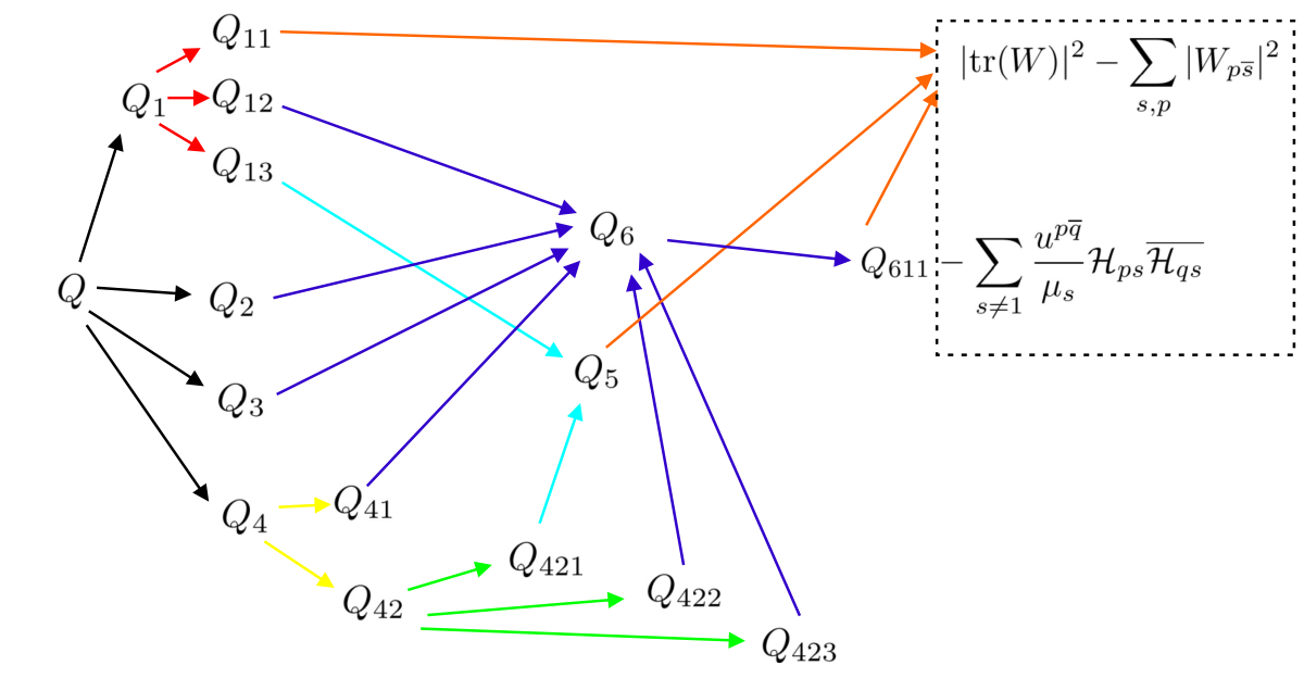
Refer to caption — Figure 1: Transformation of $Q$

(Step 1. Red Arrows in Figure 1) To simplify $Q_{1}$ , we need to use the relation between $A$ and $\mathcal{A}$ . Since

A=\mathcal{A}-h(u_{i}u_{\bar{j}}),\text{ and }\mathcal{A}=I,

(3.56)

it follows that

\displaystyle A^{-1}=I+\frac{h(u_{i}u_{\bar{j}})}{1-h\sum_{k}u_{k}u_{\bar{k}}}\overset{\triangle}{=}I+(r_{i}r_{\bar{j}}),

(3.57)

where $r_{i}=\sqrt{\frac{h}{1-h\sum_{k}u_{k}u_{\bar{k}}}}u_{i}$ and $r_{\bar{j}}=\overline{r_{j}}$ . With this structure, we get

u^{\bar{q}p}=\delta^{pq}+r_{p}r_{\bar{q}}\;\text{ and }\;A^{s\bar{t}}-\mathcal{A}^{s\bar{t}}=r_{s}r_{\bar{t}}.

(3.58)

Then

	$\displaystyle Q_{1}$	$\displaystyle=\sum_{p,q,s,t}(\delta^{pq}+r_{p}r_{\bar{q}})W_{s\bar{q}}(r_{s}r_{\bar{t}})\overline{W_{t\bar{p}}}$		(3.59)
		$\displaystyle=\sum_{p,q,s,t}\delta^{pq}W_{s\bar{q}}(r_{s}r_{\bar{t}})\overline{W_{t\bar{p}}}+\sum_{p,q,s,t}r_{p}r_{\bar{q}}W_{s\bar{q}}(r_{s}r_{\bar{t}})\overline{W_{t\bar{p}}}.$		(3.60)

Using $W_{p\bar{s}}u^{\bar{s}p}=0$ , we can simplify the second term in the above identity,

$\displaystyle\sum_{p,q,s,t}r_{p}r_{\bar{q}}W_{s\bar{q}}(r_{s}r_{\bar{t}})\overline{W_{t\bar{p}}}$	$\displaystyle=\sum_{p,q,s,t}r_{s}r_{\bar{q}}W_{s\bar{q}}(r_{p}r_{\bar{t}})\overline{W_{t\bar{p}}}$	(3.61)
	$\displaystyle=\sum_{p,q,s,t}-(u^{\bar{q}s}-\delta^{qs})W_{s\bar{q}}(u^{\bar{t}p}-\delta^{tp})W_{p\bar{t}}$	(3.62)
	$\displaystyle=-\delta^{qs}W_{s\bar{q}}\delta^{tp}W_{p\bar{t}}$	(3.63)
	$\displaystyle=\delta^{qs}W_{s\bar{q}}\delta^{tp}\overline{W_{t\bar{p}}}=\bigl\|\mathrm{tr}\bigl(W_{t\bar{q}}\bigr)\bigr\|^{2}\triangleq Q_{11}.$	(3.64)

Relabeling the summation indices in the first term of (3.60) yields

\sum_{s,t,p,q}\delta^{pq}W_{s\bar{q}}(r_{s}r_{\bar{t}})\overline{W_{t\bar{p}}}=\sum_{t\neq 1,p,q}r_{p}r_{\bar{q}}W_{p\bar{t}}\overline{W_{q\bar{t}}}+\sum_{p,q}r_{p}r_{\bar{q}}W_{p\bar{1}}\overline{W_{q\bar{1}}}.

(3.65)

We denote the two terms on the right-hand side of the above equation by $Q_{12}$ and $Q_{13}$ respectively. We lable them differently since $Q_{13}$ cancels with other terms.

(Step 2. Yellow Arrows in Figure 1) In $Q_{4}$ , terms with $s\neq 1$ should be treated differently from those with $s=1$ .

	$\displaystyle Q_{4}$	$\displaystyle=-\sum_{p,q,s}u^{{p\overline{q}}}\mathscr{B}^{(p)}_{1s}\overline{\mathscr{B}^{(q)}_{1s}}$		(3.66)
		$\displaystyle=-\sum_{s\neq 1,p,q}u^{{p\overline{q}}}\mathscr{B}^{(p)}_{1s}\overline{\mathscr{B}^{(q)}_{1s}}-\sum_{p,q}u^{{p\overline{q}}}\mathscr{B}^{(p)}_{11}\overline{\mathscr{B}^{(q)}_{11}}.$		(3.67)

Denote the last two terms by $Q_{41}$ and $Q_{42}$ respectively.

(Step 3. Green Arrows in Figure 1) Term $Q_{42}$ can be further simplified. Since $\partial_{p}\sigma\sim 0$ and at the point of computation we assume $\mathcal{K}^{1}_{1}=\mathcal{M}_{1{\overline{q}}}\mathcal{A}^{1{\overline{q}}}$ , we have

\displaystyle\partial_{p}\mathcal{M}_{1{\overline{1}}}\sim 0.

(3.68)

More explicitely, this is

\displaystyle W_{p{\overline{1}}}+h(u_{1}-u_{{\overline{1}}})\delta_{p1}-\mathscr{B}^{(p)}_{11}\sim 0.

(3.69)

This provides a relation between $W_{p{\overline{1}}}+h(u_{1}-u_{{\overline{1}}})\delta_{p1}$ and $\mathscr{B}^{(p)}_{11}$ . Plugging this into $Q_{42}$ , we get

$\displaystyle Q_{42}$	$\displaystyle\sim-u^{{p\overline{q}}}(W_{p{\overline{1}}}+h(u_{1}-u_{\overline{1}})\delta_{p1})\overline{(W_{q{\overline{1}}}+h(u_{1}-u_{\overline{1}})\delta_{q1})}$	(3.70)
	$\displaystyle=-u^{{p\overline{q}}}W_{p{\overline{1}}}\overline{W_{q{\overline{1}}}}-u^{1{\overline{q}}}h(u_{1}-u_{\overline{1}})\overline{W_{q{\overline{1}}}}-u^{p{\overline{1}}}W_{p{\overline{1}}}\overline{h(u_{1}-u_{{\overline{1}}})}$
	$\displaystyle\ \ \ \ \ \ \ \ \ \ \ \ \ \ \ \ \ \ \ \ \ \ \ \ \ \ \ \ \ \ \ \ \ \ \ \ \ \ \ \ \ \ \ \ \ \ \ \ \ \ \ \ \ \ \ \ \ \ \ \ -u^{1{\overline{1}}}\|h(u_{1}-u_{\overline{1}})\|^{2}$	(3.71)
	$\displaystyle\triangleq Q_{421}+Q_{422}+Q_{423},$	(3.72)

where

$\displaystyle Q_{421}$	$\displaystyle=-u^{{p\overline{q}}}W_{p{\overline{1}}}\overline{W_{q{\overline{1}}}},$	(3.73)
$\displaystyle Q_{422}$	$\displaystyle=-u^{1{\overline{q}}}h(u_{1}-u_{\overline{1}})\overline{W_{q{\overline{1}}}}-u^{p{\overline{1}}}W_{p{\overline{1}}}\overline{h(u_{1}-u_{{\overline{1}}})},$	(3.74)
$\displaystyle Q_{423}$	$\displaystyle=-u^{1{\overline{1}}}\|h(u_{1}-u_{\overline{1}})\|^{2}.$	(3.75)

We need to transform $Q_{422}$ using the relation $u^{{p\overline{q}}}W_{{p\overline{q}}}=0$ , which says

\displaystyle\sum_{s\neq 1}u^{p{\overline{s}}}W_{p{\overline{s}}}\sim-u^{p{\overline{1}}}W_{p{\overline{1}}}.

(3.76)

Plugging this into (3.74), we get

\displaystyle Q_{422}=\sum_{s\neq 1}u^{s{\overline{q}}}h(u_{1}-u_{\overline{1}})\overline{W_{q{\overline{s}}}}+\sum_{s\neq 1}u^{p{\overline{s}}}W_{p{\overline{s}}}\overline{h(u_{1}-u_{{\overline{1}}})}.

(3.77)

(Step 4. Blue Arrows in Figure 1) By putting $Q_{13}$ and $Q_{421}$ together we can make them simplier:

\displaystyle Q_{13}+Q_{421}=r^{p}\overline{r^{q}}W_{p{\overline{1}}}\overline{W_{q{\overline{1}}}}-u^{{p\overline{q}}}W_{p{\overline{1}}}\overline{W_{q{\overline{1}}}}=-\sum_{p}|W_{p{\overline{1}}}|^{2}.

(3.78)

(Step 5. Purple Arrows in Figure 1)

Denote that

\displaystyle Q_{6}=Q_{12}+Q_{2}+Q_{3}+Q_{41}+Q_{422}+Q_{423}.

(3.79)

In the summands on the right-hand side of (3.79), we collect all the terms which are quadratic forms of $W$ and denote their summation by $Q_{61}$ :

\displaystyle Q_{61}=\sum_{s\neq 1}W_{p{\overline{s}}}\overline{W_{q{\overline{s}}}}\left(r^{p}\overline{r^{q}}-\frac{u^{{p\overline{q}}}}{\mu_{s}}\right).

(3.80)

Using $\mu_{s}=1-b_{s}^{2}$ , the above expression can be simplified

r_{p}r_{\bar{q}}-\frac{u^{\bar{q}p}}{\mu_{s}}=r_{p}r_{\bar{q}}-u^{\bar{q}p}-\frac{u^{\bar{q}p}b_{s}^{2}}{\mu_{s}}=-\delta^{pq}-\frac{u^{\bar{q}p}b_{s}^{2}}{\mu_{s}}.

(3.81)

Then we denote $Q_{61}=Q_{611}+Q_{612}.$ Where

	$\displaystyle Q_{611}$	$\displaystyle=-\sum_{s\neq 1,p}W_{p{\overline{s}}}\overline{W_{p{\overline{s}}}},$		(3.82)
	$\displaystyle Q_{612}$	$\displaystyle=-\sum_{s\neq 1,p,q}\frac{u^{p{\overline{q}}}b_{s}^{2}}{\mu_{s}}W_{p{\overline{s}}}\overline{W_{q{\overline{s}}}}.$		(3.83)

In (3.79), we put the terms containing both $W$ and $\mathscr{B}^{(p)}$ together and denote their sum by $Q_{62}$ :

\displaystyle Q_{62}=\sum_{s\neq 1,p,q}W_{p{\overline{s}}}\overline{\mathscr{B}^{(q)}_{1s}}b_{s}\frac{u^{{p\overline{q}}}}{\mu_{s}}+\overline{W_{q{\overline{s}}}}{\mathscr{B}^{(p)}_{1s}}b_{s}\frac{u^{{p\overline{q}}}}{\mu_{s}}

(3.84)

In (3.79), we put the terms which are quadratic forms of $\mathscr{B}^{(p)}$ together and denote their summation by $Q_{63}$ :

\displaystyle Q_{63}=-\sum_{s\neq 1,p,q}u^{{p\overline{q}}}\mathscr{B}^{(p)}_{1s}\overline{\mathscr{B}^{(q)}_{1s}}-\sum_{s\neq 1,p,q}u^{{p\overline{q}}}\frac{b_{s}^{2}}{\mu_{s}}\mathscr{B}^{(p)}_{1s}\overline{\mathscr{B}^{(q)}_{1s}}.

(3.85)

On the right-hand side of the equation above, two summands are contributed by $Q_{41}$ and $Q_{3}$ respectively. Using $\mu_{s}=1-b_{s}^{2}$ , $Q_{63}$ can be simplified:

\displaystyle Q_{63}=-\sum_{s\neq 1,p,q}\frac{u^{{p\overline{q}}}}{\mu_{s}}\mathscr{B}^{(p)}_{1s}\overline{\mathscr{B}^{(q)}_{1s}}.

(3.86)

In (3.79), we put the terms which contain both $h(u_{1}-u_{\overline{1}})$ and $W$ together and denote their summation by $Q_{64}$ :

	$\displaystyle Q_{64}=$	$\displaystyle\left(\sum_{s\neq 1,q}u^{s{\overline{q}}}\overline{W_{q{\overline{s}}}}{h(u_{1}-u_{\overline{1}})}+\sum_{s\neq 1,q}u^{p{\overline{s}}}{W_{p{\overline{s}}}}\overline{h(u_{1}-u_{{\overline{1}}})}\right)$
		$\displaystyle\ -\left(\sum_{s\neq 1,q}\frac{u^{s{\overline{q}}}}{\mu_{s}}\overline{W_{q{\overline{s}}}}{h(u_{1}-u_{\overline{1}})}+\sum_{s\neq 1,q}\frac{u^{p{\overline{s}}}}{\mu_{s}}{W_{p{\overline{s}}}}\overline{h(u_{1}-u_{{\overline{1}}})}\right).$		(3.87)

Terms in the two brackets in the equation above are contributed by $Q_{422}$ and $Q_{3}$ respectively. Using $\mu_{s}=1-b_{s}^{2}$ , $Q_{64}$ can be simplified:

\displaystyle Q_{64}=-\left(\sum_{s\neq 1,q}\frac{u^{s{\overline{q}}}b_{s}^{2}}{\mu_{s}}\overline{W_{q{\overline{s}}}}{h(u_{1}-u_{\overline{1}})}+\sum_{s\neq 1,q}\frac{u^{p{\overline{s}}}b_{s}^{2}}{\mu_{s}}{W_{p{\overline{s}}}}\overline{h(u_{1}-u_{{\overline{1}}})}\right).

(3.88)

In (3.79), we put the terms which contain both $h(u_{1}-u_{\overline{1}})$ and $\mathscr{B}^{(p)}$ together and denote their summation by $Q_{65}$ :

\displaystyle Q_{65}=-\left(\sum_{s\neq 1,q}\frac{u^{s{\overline{q}}}b_{s}}{\mu_{s}}\overline{\mathscr{B}^{(q)}_{1s}}{h(u_{1}-u_{\overline{1}})}+\sum_{s\neq 1,q}\frac{u^{p{\overline{s}}}b_{s}}{\mu_{s}}{\mathscr{B}^{(p)}_{1s}}\overline{h(u_{1}-u_{{\overline{1}}})}\right).

(3.89)

In (3.79), we put the terms which contain only $h(u_{1}-u_{\overline{1}})$ together and denote their summation by $Q_{66}$ :

\displaystyle Q_{66}=|h(u_{1}-u_{\overline{1}})|^{2}\sum_{s}u^{s{\overline{s}}}-|h(u_{1}-u_{\overline{1}})|^{2}\sum_{s\neq 1}\frac{u^{s{\overline{s}}}}{\mu_{s}}-|h(u_{1}-u_{\overline{1}})|^{2}u^{1{\overline{1}}}.

(3.90)

Three terms on the right-hand side of (3.90) are contributed by $Q_{2},Q_{3},Q_{23}$ respectively. After cancellation and simplification, we get

\displaystyle Q_{66}=-|h(u_{1}-u_{\overline{1}})|^{2}\sum_{s\neq 1}\frac{u^{s{\overline{s}}}b_{s}^{2}}{\mu_{s}}.

(3.91)

By choosing

\displaystyle H_{ps}=W_{p{\overline{s}}}b_{s}-\mathscr{B}^{(p)}_{1s}+h(u_{1}-u_{\overline{1}})\delta_{sp}b_{s},

(3.92)

we find $Q_{6}-Q_{611}$ can be largely simplifed as

\displaystyle Q_{6}-Q_{611}=-\sum_{s\neq 1,p,q}\frac{u^{p{\overline{q}}}}{\mu_{s}}H_{ps}\overline{H_{qs}}.

(3.93)

Comparing (3.50) and (3.92), we find $H_{ps}$ is exactly $\partial_{p}{\mathcal{M}_{s{\overline{1}}}}$ .

(Step 6. Orange Arrows in Figure 1)

	$\displaystyle Q_{11}+Q_{5}+Q_{611}$	$\displaystyle=\|{\text{tr}}(W)\|^{2}-\sum_{p}\|W_{p{\overline{1}}}\|^{2}-\sum_{s\neq 1,p}\|W_{p\overline{s}}\|^{2}$		(3.94)
		$\displaystyle=\|{\text{tr}}(W)\|^{2}-\sum_{s,p}\|W_{p\overline{s}}\|^{2}.$		(3.95)

Finally, we get

\displaystyle Q

\displaystyle\sim\bigl|\mathrm{tr}\bigl(W\bigr)\bigr|^{2}-\sum_{p,s}|W_{p\bar{s}}|^{2}-\sum_{s\neq 1,q,p}\frac{u^{\bar{q}p}}{\mu_{s}}H_{ps}\overline{H_{qs}},

(3.96)

which is in the dashed square in Figure 1. In addition, we have

\displaystyle u^{p{\overline{q}}}\partial_{{p\overline{q}}}\sigma\sim\bigl|\mathrm{tr}\bigl(W\bigr)\bigr|^{2}-\sum_{p,s}|W_{p\bar{s}}|^{2}-2\sum_{s\neq 1,q,p}\frac{u^{\bar{q}p}}{\mu_{s}}H_{ps}\overline{H_{qs}}.

(3.97)

3.2 Proving Non-Positivity in the Case of Complex Dimension 2

So we want to prove that for any anti-Hermitian matrix $(W_{p\bar{s}})$ ,

\displaystyle\sum_{p,s}W_{p\bar{s}}\overline{W_{p\bar{s}}}-\bigl|\mathrm{tr}\bigl(W_{p\bar{s}}\bigr)\bigr|^{2}\geq 0,

(3.98)

with the restriction

\displaystyle\sum_{p,q}W_{p\bar{q}}u^{\bar{q}p}=\sum_{p,q}W_{p\bar{q}}(\delta^{\bar{q}p}+r_{p}r_{\bar{q}})=0.

(3.99)

It turns out that this is valid only in complex dimension two. When the complex dimension is greater than two, the quadratic form (modulo (3.99)) may not be positive definite. In the following, we prove this in the case of complex dimension two. Denote

(W_{p\bar{s}})=\begin{pmatrix}\sqrt{-1}a&\sqrt{-1}b+d\\ \sqrt{-1}b-d&\sqrt{-1}c\end{pmatrix},

(3.100)

where $a,b,c,d$ are real numbers. Let $r_{1}=w_{1}+\sqrt{-1}v_{1}$ and $r_{2}=w_{2}+\sqrt{-1}v_{2}$ . Then

		$\displaystyle(u^{\bar{q}p})=\begin{pmatrix}1+r_{1}\overline{r_{1}}&r_{1}\overline{r_{2}}\\ \overline{r_{2}}r_{1}&1+r_{2}\overline{r_{2}}\end{pmatrix}$
		$\displaystyle=\begin{pmatrix}1+w_{1}^{2}+v_{1}^{2}&w_{1}w_{2}+v_{1}v_{2}+\sqrt{-1}(v_{1}w_{2}-w_{1}v_{2})\\ w_{1}w_{2}+v_{1}v_{2}-\sqrt{-1}(v_{1}w_{2}-w_{1}v_{2})&1+w_{2}^{2}+v_{2}^{2}\end{pmatrix}.$

Relation (3.98) is equivalent to

a^{2}+c^{2}+2b^{2}+2d^{2}\geq(a+c)^{2}.

(3.101)

Expanding the right-hand side and cancelling $a^{2}$ and $c^{2}$ , we obtain

b^{2}+d^{2}\geq ac.

(3.102)

Relation (3.99) is equivalent to

a(1+w_{1}^{2}+v_{1}^{2})+c(1+w_{2}^{2}+v_{2}^{2})+2b(w_{1}w_{2}+v_{1}v_{2})-2d(v_{1}w_{2}-w_{1}v_{2})=0.

(3.103)

Using this relation in (3.102), we replace $a$ by a combination of $b,c,d$ , and transform (3.102) into

(b^{2}+d^{2})(1+w_{1}^{2}+v_{1}^{2})\geq-c^{2}(1+w_{2}^{2}+v_{2}^{2})-2bc(w_{1}w_{2}+v_{1}v_{2})+2dc(v_{1}w_{2}-w_{1}v_{2}).

It is equivalent to the positive semi-definiteness of the following matrix

\begin{pmatrix}1+w_{2}^{2}+v_{2}^{2}&w_{1}w_{2}+v_{1}v_{2}&w_{1}v_{2}-v_{1}w_{2}\\ w_{1}w_{2}+v_{1}v_{2}&1+w_{1}^{2}+v_{1}^{2}&0\\ w_{1}v_{2}-v_{1}w_{2}&0&1+w_{1}^{2}+v_{1}^{2}\end{pmatrix}.

(3.104)

According to Lemma A.2, it suffices to show that the following quantity is nonnegative:

(1+w_{1}^{2}+v_{1}^{2})(1+w_{2}^{2}+v_{2}^{2})-(w_{1}w_{2}+v_{1}v_{2})^{2}-(v_{1}w_{2}-w_{1}v_{2})^{2}\geq 0.

(3.105)

With basic computation, the above inequality equals to

1+w_{1}^{2}+v_{1}^{2}+w_{2}^{2}+v_{2}^{2}>0.

(3.106)

So the matrix in (3.104) is positive definite and we have proved that (3.98) is nonnegative.

Remark 2.

The condition (3.98) may not be valid in general dimension. For example, in the case of dimension n, let

W_{p\bar{s}}=\begin{cases}\sqrt{-1}\delta_{ps},&p>1,\\ -(n-1)\frac{\sqrt{-1}}{C^{2}+1}\delta_{ps},&p=1.\end{cases}

(3.107)

Let $r_{1}=C$ , $r_{k}=0$ for $k>1$ , where $C$ is a real constant. Then $(W_{p\bar{s}})$ is skew-Hermitian and the condition (3.99) is satisfied. Under this setting, we obtain

\mathrm{tr}(W_{p\bar{s}})=(n-1)\sqrt{-1}(1-\frac{1}{C^{2}+1}).

(3.108)

So the condition (3.98) becomes

(n-1)+\frac{(n-1)^{2}}{(C^{2}+1)^{2}}-\left[(n-1)\left(1-\frac{1}{C^{2}+1}\right)\right]^{2}\geq 0.

(3.109)

This is equivalent to

n-1-(n-1)^{2}+\frac{2(n-1)^{2}}{C^{2}+1}=n-1+(n-1)^{2}\left(\frac{2}{C^{2}+1}-1\right)\geq 0.

(3.110)

It is only valid for $n=1$ and $n=2$ . When $n>1$ , the inequality (3.110) is equivalent to

1\geq(n-1)\left(1-\frac{2}{C^{2}+1}\right).

(3.111)

For any fixed $n>2$ , we can choose $C$ large enough, such that

1<(n-1)\left(1-\frac{2}{C^{2}+1}\right).

(3.112)

Remark 3.

After showing that $|{\text{tr}}(W)|^{2}-\sum_{p,s}W_{p\bar{s}}\overline{W_{p\bar{s}}}$ may not be non-positive in general dimesion, the readers may still wander if this is true for $u^{p\overline{q}}\sigma_{p\bar{q}}$ . Since

\displaystyle u^{p\overline{q}}\sigma_{p\bar{q}}\sim|{\text{tr}}(W)|^{2}-\sum_{p,s}W_{p\bar{s}}\overline{W_{p\bar{s}}}-2\sum_{s\neq 1,q,p}\frac{u^{\bar{q}p}}{\mu_{s}}H_{ps}\overline{H_{qs}},

(3.113)

it’s reasonable to ask if the subtraction of $-2\sum_{s\neq 1,q,p}\frac{u^{\bar{q}p}}{\mu_{s}}H_{ps}\overline{H_{qs}}$ makes a difference. The answer is negative. In the following situation the contribution of $-2\sum_{s\neq 1,q,p}\frac{u^{\bar{q}p}}{\mu_{s}}H_{ps}\overline{H_{qs}}$ is zero.

Let $b_{s}=0$ for $s\neq 1$ , which is a possible situation. In this situation

\displaystyle u^{p\overline{q}}\sigma_{p\bar{q}}\sim|{\text{tr}}(W)|^{2}-\sum_{p,s}W_{p\bar{s}}\overline{W_{p\bar{s}}}-2\sum_{s\neq 1,q,p}\frac{u^{\bar{q}p}}{\mu_{s}}\mathscr{B}^{(p)}_{1s}\overline{\mathscr{B}^{(q)}_{1s}}.

(3.114)

$W$ is the same as that of the previous remark. We notice that $W$ is diagonal. The only relation between $\mathscr{B}^{(p)}$ and $W$ is (3.69), which put a restriction on $W_{p{\overline{1}}}$ and $\mathscr{B}^{(p)}_{11}$ . Also we notice that $\mathscr{B}^{(p)}_{1s}=\mathscr{B}^{(s)}_{1p}$ , so

\displaystyle-2\sum_{s\neq 1,q,p}\frac{u^{\bar{q}p}}{\mu_{s}}\mathscr{B}^{(p)}_{1s}\overline{\mathscr{B}^{(q)}_{1s}}=-2\sum_{s\neq 1,q,p}\frac{u^{\bar{q}p}}{\mu_{s}}\mathscr{B}^{(s)}_{1p}\overline{\mathscr{B}^{(s)}_{1q}},

(3.115)

and terms related to $W$ are

\displaystyle-2\sum_{s\neq 1}\frac{u^{\bar{1}1}}{\mu_{s}}\mathscr{B}^{(s)}_{11}\overline{\mathscr{B}^{(s)}_{11}}=-2\sum_{s\neq 1}|W_{1s}|^{2}.

(3.116)

By our choice, all the off-diagonal elements of $W$ are $0$ , so the contribution above is $0$ .

So, we get at the place where the minimum eigenvalue of $\mathcal{K}<$ the second minimum eigenvalue of $\mathcal{K}$

\displaystyle u^{{i\overline{j}}}\partial_{{i\overline{j}}}\sigma\leq C_{0}(\sigma+|\nabla\sigma|).

(3.117)

This result implies the following proposition, which is crucial in the lower bound estimate for $\sigma$ :

Proposition 1.

At the place where the minimum eigenvalue of $\mathcal{K}<$ the second minimum eigenvalue of $\mathcal{K}$ , $\sigma$ cannot achieve a $0$ local minimum, unless $\sigma\equiv 0$ .

Proof.

When the minimum eigenvalue of $\mathcal{K}<$ the second minimum eigenvalue of $\mathcal{K}$ , $\sigma$ is a smooth function and it satisfies (3.117). The result follows from Harnak inequality. ∎

3.3 The General Case via Approximation

Proposition 1 in the previous section cannot directly provide a lower bound estimate for $\sigma$ . As a function defined in $\Omega$ , $\sigma$ is in general only $C^{0}$ and at the place where $\sigma$ achieves a local minimum, the minimum eigenvalue of $\mathcal{K}$ may equal to the second minimum eigenvalue of $\mathcal{K}$ . In this section, we perturb $\sigma$ by quadratic polynomials and get $\sigma^{\epsilon}$ . We will show that when $\sigma^{\epsilon}$ achieves a local minimum at a point $z_{0}$ , we do have that the minimum eigenvalue of $\mathcal{K}^{q}(z_{0})<$ the second minimum eigenvalue of $\mathcal{K}^{q}(z_{0})$ , where $\mathcal{K}^{q}$ is computed using $u+q$ (parallel to that $\mathcal{K}$ is computed using $u$ ) where $q$ is a pluriharmonic quadratic polynomial with $L^{2}$ norm restriction.

Since $\Omega$ is a strictly convex domain with smooth boundary and $u$ is $C^{2}$ continuous with nonvanishing gradient near $\partial\Omega$ , $u$ has strictly convex level sets near $\partial\Omega$ . So for a small enough $\varepsilon$ , with

\displaystyle\Omega^{\varepsilon}=\left\{z\in\Omega|\ \text{dist}(z,\partial\Omega)>\varepsilon\right\}

(3.118)

$-\sqrt{-u}$ is strictly convex on $\partial\Omega^{\varepsilon}$ . In the following, we show that $-\sqrt{-u}$ is stricly convex in $\Omega^{\varepsilon}$ , and we need to first derive an apriori estimate.

Let

\displaystyle\mathscr{Q}^{\epsilon}=\left\{q\left|\ \text{quadratic polynomial, }q_{{i\overline{j}}}=0,\ \int_{B_{1}({\bf{a}})}q^{2}\leq\right.\epsilon\right\}.

(3.119)

In above, $B_{1}({\bf{a}})$ is a ball of radius $1$ with respect to the standard metric on $\mathbb{C}^{n}$ , with center ${\bf{a}}\in\Omega$ ; the integration also uses the standard measure on $\mathbb{C}^{n}$ .

Proposition 2.

Suppose that $u<0$ and $-\sqrt{-u}$ is strictly convex in $\overline{\Omega^{\varepsilon}}$ . $\epsilon$ is small enough so that for any $q\in\mathscr{Q}^{\epsilon}$ ,

		$\displaystyle\ \ \ \ \ \ u+q<0,$	$\displaystyle\text{ \ \ \ \ \ in \ }\overline{\Omega^{\varepsilon}},$		(3.120)
		$\displaystyle u+q\text{ is strictly pluri-subharmonic},$	$\displaystyle\text{ \ \ \ \ \ in \ }\overline{\Omega^{\varepsilon}},$		(3.121)

and

\displaystyle-\sqrt{-u-q}\text{ is strictly convex on }\partial{\Omega^{\varepsilon}}.

(3.122)

Then for any $q\in\mathscr{Q}^{\epsilon}$

\displaystyle-\sqrt{-u-q}\text{ is strictly convex in }{\Omega^{\varepsilon}}.

(3.123)

In addition, we can find a constant $C$ depending on $\epsilon$ , $\min_{\overline{\Omega^{\varepsilon}}}u$ , $\max_{\overline{\Omega^{\varepsilon}}}u$ and the diameter of $\Omega$ , so that

\displaystyle\text{the real Hessian of }-\sqrt{-u}>CI_{2n}.

(3.124)

Proof of the Proposition 2.

Given $q\in\mathscr{Q}^{\epsilon}$ , let

	$\displaystyle\mathcal{A}^{q}=\left[(u+q)_{i\overline{j}}+\frac{(u+q)_{i}(u+q)_{\overline{j}}}{2(-u-q)}\right];$		(3.125)
	$\displaystyle\mathcal{B}^{q}=\left[(u+q)_{ij}+\frac{(u+q)_{i}(u+q)_{j}}{2(-u-q)}\right],$		(3.126)

and $\mathcal{M}^{q}=\mathcal{A}^{q}-\mathcal{B}^{q}(\overline{\mathcal{A}^{q}})^{-1}\overline{\mathcal{B}^{q}},\ \mathcal{K}^{q}=\mathcal{M}^{q}(\mathcal{A}^{q})^{-1}.$ In above that $\mathcal{A}^{q}$ is invertible is guaranteed by the assumption (3.121). Denote

$\displaystyle{\lambda_{1}}(\mathcal{K}^{q})(z_{0})$	$\displaystyle=\text{ the minimum eigenvalue of }\mathcal{K}^{q}(z_{0}),$	(3.127)
$\displaystyle{\lambda_{2}}(\mathcal{K}^{q})(z_{0})$	$\displaystyle=\text{ the second minimum eigenvalue of }\mathcal{K}^{q}(z_{0}),$	(3.128)
$\displaystyle\sigma^{\epsilon}(z_{0})$	$\displaystyle=\min_{q\in\mathscr{Q}^{\epsilon}}{\lambda_{1}}(\mathcal{K}^{q}(z_{0})).$	(3.129)

Since $\mathscr{Q}^{\delta_{1}}\subset\mathscr{Q}^{\delta_{2}}$ when ${\delta_{1}}\leq{\delta_{2}}$ , $\sigma^{\delta_{1}}\geq\sigma^{\delta_{2}}$ . So $\sigma^{s}$ depends on $s$ monotonically. Since ${\lambda_{1}}(\mathcal{K}^{q})$ depends on $q$ algebraically and $\mathcal{A}^{q}$ is invertible for $q\in\mathscr{Q}^{\epsilon}$ , we have that at any fixed point $z_{0}$ , $\sigma^{s}(z_{0})$ is a continuous function of $s$ for $s\leq\epsilon$ .

At any point $z_{0}\in\overline{\Omega^{\varepsilon}}$ , since $\mathscr{Q}^{\epsilon}$ is closed and of finite dimension, we can find $r\in\mathscr{Q}^{\epsilon}$ so that

\displaystyle\lambda_{1}(\mathcal{K}^{r})(z_{0})=\sigma^{\epsilon}(z_{0}),

(3.130)

and for $z\neq z_{0}$

\displaystyle\lambda_{1}(\mathcal{K}^{r})(z)\geq\sigma^{\epsilon}(z).

(3.131)

This means the graph of $\lambda_{1}(\mathcal{K}^{r})$ contacts with the graph of $\sigma^{\epsilon}$ from above. In addition, Lemma A.3 implies

\displaystyle\lambda_{1}(\mathcal{K}^{r})(z_{0})<\lambda_{2}(\mathcal{K}^{r})(z_{0}).

(3.132)

So $\lambda_{1}(\mathcal{K}^{r})$ is a smooth function around $z_{0}$ . Also since $u+r$ is still a solution to the Monge-Ampère equation, $\det\left((u+r)_{{p\overline{q}}}\right)=1$ , ${\lambda_{1}}(\mathcal{K}^{r})$ also satisfy (3.117) with $C_{0}$ depending on $u+r$ .

Remark 4.

The graph of $\sigma^{\epsilon}$ is the lower envelop of a family of locally defined smooth functions ( ${\lambda_{1}}(\mathcal{K}^{r})$ defined around $z_{0}$ ) satisfying (3.117) with $C_{0}$ depending on $u+r$ . But we cannot say that $\sigma^{\epsilon}$ satisfies

\displaystyle u^{{i\overline{j}}}\partial_{{i\overline{j}}}\sigma^{\epsilon}\leq C_{1}(\sigma^{\epsilon}+|\nabla\sigma^{\epsilon}|)

(3.133)

in the sense of viscosity because it’s not obvious why we can find a uniform $C_{1}$ depending on $u$ and $\epsilon$ .

The assumption (3.122) implies that $\sigma^{\epsilon}>0$ on $\partial\Omega^{\varepsilon}$ . If $\sigma^{\epsilon}$ is not positive in $\Omega^{\varepsilon}$ , then for a $\delta\leq\epsilon$ , $\sigma^{\delta}$ achieves a $0$ local minimum at a point $z_{1}\in\Omega^{\varepsilon}$ . Then for a $q\in\mathscr{Q}^{\delta}$ , $\lambda_{1}(\mathcal{K}^{q})$ achieves a $0$ local minimum at $z_{1}$ . Since $\lambda_{1}(\mathcal{K}^{q})$ cannot achieve $0$ interior local minimum according to Proposition 1, we get a contradiction. So we proved that $\sigma^{\epsilon}>0$ in $\Omega^{\varepsilon}$ . It follows that for any $q\in\mathscr{Q}^{\epsilon}$ , ${\lambda_{1}}(\mathcal{K}^{q})>0$ and $-\sqrt{-u-q}$ is strictly convex. Using Lemma A.4, we have a convexity estimate for $-\sqrt{-u}$ . This proves the proposition. ∎

For a smooth and strictly convex domain $\Omega$ , we connect it with a ball. Let

\displaystyle\Omega_{t}=t\Omega+(1-t)B,

(3.134)

where $B$ is a ball of radius 1. Let $u_{t}$ be the solution to the following Dirichlet problem:

\displaystyle u_{t}=0,\ \ \ \ \ \text{on }\partial\Omega_{t},

(3.135)

and

\displaystyle det(\partial_{{i\overline{j}}}u_{t})=1,\text{\ \ \ \ \ \ in }\Omega_{t}.

(3.136)

In particular, we have $u_{0}=|z|^{2}-1$ and $u_{1}=u$ . We can find a small $\varepsilon>0$ , so that $-\sqrt{-u_{t}}$ is strictly convex on $\partial\Omega^{\varepsilon}_{t}$ for all $t\in[0,1]$ . For each $t$ , we can compute $\sigma^{\epsilon}_{t}$ using $u_{t}$ , parallel to the previous computation, replacing $u$ by $u_{t}$ . Then for a fixed $\epsilon$ small enough $\sigma^{\epsilon}_{t}>0$ on $\partial\Omega^{\varepsilon}_{t}$ and $u_{t}+q$ is strictly plurisubharmonic for $q\in\mathscr{Q}^{\epsilon}$ and for all $t\in[0,1]$ .

Let $m(t)=\text{min}_{\overline{\Omega^{\varepsilon}_{t}}}\sigma^{\epsilon}_{t}$ . Then $m(t)$ is a continuous function of $t$ , with $m(0)>0$ . If $m(1)>0$ , $-\sqrt{-u}$ is strictly convex and the result is proved. Otherwize, let $s_{0}=\min\left\{s|m(s)=0\right\}.$ For $s<s_{0}$ , $\sigma_{s}^{\epsilon}>0$ . So for $q\in\mathscr{Q}^{\epsilon}$ , $u_{s}+q$ is strictly convex. Lemma A.4 implies a convexity estimate for $-\sqrt{-u_{s}}$ , with $s<s_{0}$ , depending on $\epsilon$ and the diameter of $\Omega$ . Taking limit, we know $-\sqrt{-u_{s_{0}}}$ is strictly convex. This allow us to apply Proposition 2 to $u_{s_{0}}$ . So $\sigma_{s_{0}}^{\epsilon}>0$ in $\Omega^{\varepsilon}_{s_{0}}$ , which is a contradiction.

Therefore $m(1)>0$ , $-\sqrt{-u}$ is strictly convex and the convexity estimate follows from Lemma A.4.

Appendix A Algebra Lemmas

Lemma A.1.

Suppose that $u$ is a quadratic polynomial on $\mathbb{C}^{n}$ . Let $A=(u_{i\bar{j}})$ and $B=(u_{ij})$ . Here $u_{i\bar{j}}$ and $u_{ij}$ are derivatives with respect to the complex coordinates $z^{i}$ . Let $D$ be the real Hessian matrix of $u$ :

\begin{pmatrix}D_{2i-1,2j-1}&D_{2i-1,2j}\\ D_{2i,2j-1}&D_{2i,2j}\end{pmatrix}=\begin{pmatrix}\partial_{x^{i}}\partial_{x^{j}}u&\partial_{x^{i}}\partial_{y^{j}}u\\ \partial_{y^{i}}\partial_{x^{j}}u&\partial_{y^{i}}\partial_{y^{j}}u\end{pmatrix},

(A.1)

where $x^{i}+\sqrt{-1}y^{i}=z^{i}$ . Then

\det\left(I-B\overline{A}^{-1}\overline{B}A^{-1}\right)=\frac{\det D}{4^{n}\left(\det A\right)^{2}}.

(A.2)

Proof.

Firstly, we show that the identity above is invariant under a linear change of coordinates. Then we choose complex coordinates so that $A=I$ and $B=\mathrm{diag}(b_{1},b_{2},\cdots,b_{n})$ , with $b_{k}\in\mathbb{R}$ , and we prove the identity (A.2) in this case.

Let $\{\widetilde{z^{i}}=z^{j}K^{i}_{j}\}$ be another set of coordinates. Then $\widetilde{A}=(\partial_{\widetilde{z^{i}}}\overline{\partial_{\widetilde{z^{j}}}}u)$ , $\widetilde{B}=(\partial_{\widetilde{z^{i}}}\partial_{\widetilde{z^{j}}}u)$ , and $\widetilde{D}$ be the real Hessian matrix of $u$ with coordinates $(\widetilde{x^{i}},\widetilde{y^{i}})$ with $\widetilde{x^{i}}+\sqrt{-1}\widetilde{y^{i}}=\widetilde{z^{i}}$ . We have $A=K\widetilde{A}K^{*}$ and $B=K\widetilde{B}K^{T}$ . Then

B\overline{A}^{-1}\overline{B}A^{-1}=K\left(\widetilde{B}\overline{\widetilde{A}}^{-1}\overline{\widetilde{B}}\widetilde{A}\right)K^{-1}.

(A.3)

When the coordinates are changed, the matrix $B\overline{A}^{-1}\overline{B}A^{-1}$ transforms by a similarity transformation. Consequently, the matrices $B\overline{A}^{-1}\overline{B}A^{-1}$ and $\widetilde{B}\overline{\widetilde{A}}^{-1}\overline{\widetilde{B}}\widetilde{A}$ have the same eigenvalues. Therefore, the left-hand side of (A.2) is invariant under a linear change of coordinates.

Set $K=P+\sqrt{-1}Q$ . Under this notation, the matrices $D$ and $\widetilde{D}$ satisfy the following relation:

D=R\widetilde{D}R^{T},

(A.4)

with

\begin{pmatrix}R^{2i-1,2j-1}&R^{2i-1,2j}\\ R^{2i,2j-1}&R^{2i,2j}\end{pmatrix}=\begin{pmatrix}P^{i}_{j}&-Q^{i}_{j}\\ Q^{i}_{j}&P^{i}_{j}\end{pmatrix}.

(A.5)

With the new coordinate $\widetilde{z^{i}}=\widetilde{x^{i}}+\sqrt{-1}\widetilde{y^{i}}$ , the right-hand side of (A.2) becomes

\frac{\det\widetilde{D}}{4^{n}(\det\widetilde{A})^{2}}=\frac{\det D|\det K|^{4}}{4^{n}(\det A)^{2}(\det R)^{2}}.

(A.6)

We need to show $|\det K|^{4}=(\det R)^{2}$ . This is a basic linear algebraic fact and its proof can be found in [HJ13], 1.3, p21 (d). Therefore, the right-hand side of (A.2) is invariant under a linear change of coordinate.

We first choose a coordinate such that $A=I$ . Then we choose a unitary coordinate transformation so that $B=\mathrm{diag}(b_{1},b_{2},\cdots,b_{n})$ , with $b_{k}\in\mathbb{R}$ . This is possible according to Autonne-Takagi Factorization ( Lemma A.3 of [H25]) or Corollary 4.4.4(c) of [HJ13].

In this case, we have

I-B\overline{A}^{-1}\overline{B}A^{-1}=\mathrm{diag}(1-b_{1}^{2},1-b_{2}^{2},\cdots,1-b_{n}^{2}),

(A.7)

and

D=\mathrm{diag}\left(2(1+b_{1}),2(1-b_{1}),\cdots,2(1+b_{n}),2(1-b_{n})\right).

(A.8)

It follows that

\det(I-B\overline{A}^{-1}\overline{B}A^{-1})=\Pi_{k=1}^{n}(1-b_{k}^{2})=\frac{\det D}{4^{n}}=\frac{\det D}{4^{n}(\det A)^{2}}.

(A.9)

This proves (A.2). ∎

Lemma A.2.

Let constants $B,C>0$ and $A,\beta,\gamma\in\mathbb{R}$ . The matrix

M=\begin{pmatrix}A&\beta&\gamma\\ \beta&B&0\\ \gamma&0&C\end{pmatrix}

(A.10)

is positive semi-definite if and only if

A-\frac{\beta^{2}}{B}-\frac{\gamma^{2}}{C}\geq 0.

(A.11)

Proof.

Let the matrix

P=\begin{pmatrix}1&0&0\\ -\frac{\beta}{B}&1&0\\ -\frac{\gamma}{C}&0&1\end{pmatrix},

(A.12)

which is invertible. It follows that

P^{T}MP=\begin{pmatrix}A-\frac{\beta^{2}}{B}-\frac{\gamma^{2}}{C}&0&0\\ 0&B&0\\ 0&0&C\end{pmatrix}.

(A.13)

Since congruence by an invertible matrix preserves positive semi-definiteness, we obtain

M\geq 0,\quad\text{ if and only if }\quad P^{T}MP\geq 0.

(A.14)

Moreover, since $B,C>0$ , the matrix $P^{T}MP\geq 0$ is equivalent to

A-\frac{\beta^{2}}{B}-\frac{\gamma^{2}}{C}\geq 0.

(A.15)

∎

The following lemma is used when doing the perturbation in section 3.3. It says the perturbation which minimizes the minimal eigenvalue of $\mathcal{K}^{q}$ must make the minimal eigenvalue of $\mathcal{K}^{q}$ strictly smaller than then second minimal eigenvalue of $\mathcal{K}^{q}$ .

Lemma A.3.

$u$ is a $C^{2}$ , negative function with $-\sqrt{-u}$ being strictly convex, defined in a neighborhood of $z_{0}\in\mathbb{C}^{n}$ . $\mathscr{Q}^{\epsilon}$ is a set of pluriharmonic quadratic polynomials on $\mathbb{C}^{n}$ with $L^{2}$ norm restriction:

\displaystyle\mathscr{Q}^{\epsilon}=\left\{q\big|\text{real-valued quadratic polynomial, }q_{{i\overline{j}}}=0,\ \int_{{\bf K}}q^{2}\leq\epsilon\right\}.

(A.16)

In above ${\bf K}$ is a bounded and closed set in $\mathbb{C}^{n}$ with smooth boundary; the integration uses a measure that is equivalent to the standard metric on $\mathbb{C}^{n}$ . Let

	$\displaystyle\mathcal{A}^{q}=\left[(u+q)_{i\overline{j}}+\frac{(u+q)_{i}(u+q)_{\overline{j}}}{2(-u-q)}\right](z_{0});$		(A.17)
	$\displaystyle\mathcal{B}^{q}=\left[(u+q)_{ij}+\frac{(u+q)_{i}(u+q)_{j}}{2(-u-q)}\right](z_{0}).$		(A.18)

Then we combine them to get $\mathcal{M}^{q}$ and $\mathcal{K}^{q}$ :

	$\displaystyle\mathcal{M}^{q}$	$\displaystyle=\mathcal{A}^{q}-\mathcal{B}^{q}(\overline{\mathcal{A}^{q}})^{-1}\overline{\mathcal{B}^{q}};$		(A.19)
	$\displaystyle\mathcal{K}^{q}$	$\displaystyle=\mathcal{M}^{q}(\mathcal{A}^{q})^{-1}.$		(A.20)

If $\epsilon$ is small enough so that for any $q\in\mathscr{Q}^{\epsilon}$

\displaystyle u+q<0,\ \ \ \text{\ \ at }z_{0}

(A.21)

and

\displaystyle-\sqrt{-u-q}\text{ is convex and strictly pluri-subharmonic at $z_{0}$},

(A.22)

then the $q\in\mathscr{Q}^{\epsilon}$ which minimizes the minimal eigenvalue of $\mathcal{K}^{q}$ makes

\displaystyle\text{Minimal Eigenvalue}(\mathcal{K}^{q})<\text{Second Minimal Eigenvalue}(\mathcal{K}^{q}).

(A.23)

Proof.

In the proof of this lemma, we denote the minimum eigenvalue and the second minimal eigenvalue of a matrix $H$ by ${\lambda_{1}}(H)$ and ${\lambda_{2}}(H)$ respectively. Also, in the integration, we ignore the region ${\bf K}$ since we only do integration in this region.

We prove this lemma by contradiction. Suppose that $q\in\mathscr{Q}^{\epsilon}$ minimizes ${\lambda_{1}}(\mathcal{K}^{q})$ , i.e.

\displaystyle{\lambda_{1}}(\mathcal{K}^{q})=\min_{r\in\mathscr{Q}^{\epsilon}}{\lambda_{1}}(\mathcal{K}^{r}),

(A.24)

and

\displaystyle{\lambda_{1}}(\mathcal{K}^{q})={\lambda_{2}}(\mathcal{K}^{q}).

(A.25)

Then we derive a contradiction. Note that for each fixed $\epsilon$ , $\mathscr{Q}^{\epsilon}$ is a closed set of finite dimension and $\lambda_{1}(\mathcal{K}^{q})$ is a continuous function of $q$ so a $q$ satisfying (A.24) exists.

To simplify the computation, we change coordinate on $\mathbb{C}^{n}$ linearly so that

	$\displaystyle\mathcal{A}^{q}$	$\displaystyle=I_{n};$		(A.26)
	$\displaystyle\mathcal{B}^{q}$	$\displaystyle=\text{diag}(b_{1},b_{2},\ ...\ ,b_{n}),$		(A.27)

where $1\geq b_{1}\geq b_{2}\geq\ ...\ \geq b_{n}\geq 0$ . This is possible because as we change coordinate linearly on $\mathbb{C}^{n}$ , matrices $\mathcal{A}^{q}$ and $\mathcal{B}^{q}$ change in the following way:

\mathcal{A}^{q}\rightarrow P\mathcal{A}^{q}P^{\ast},\ \ \ \mathcal{B}^{q}\rightarrow P\mathcal{B}^{q}P^{T},

where $P$ is the coordinate transition matrix. Then using Autonne-Takagi factorization, we can diagonalize $\mathcal{A}^{q}$ and $\mathcal{B}^{q}$ simultaneously, where $\mathcal{B}^{q}$ becomes diagonal with non-negative diagonal elements (see Lemma A.3 in [H25] or Corollary 4.4.4(c) in [HJ13]). Then

\displaystyle\mathcal{K}^{q}=\text{diag}(1-b_{1}^{2},\ 1-b_{2}^{2},\ ...\ ,1-b_{n}^{2}).

(A.28)

Using Lemma A.1, we know that the assumption (A.22) implies $1-b_{i}^{2}\geq 0$ . So all $b_{i}$ ’s are $\leq 1$ . Because of the assumption (A.25), we have $b_{1}=b_{2}$ .

Choose quadratic polynomials $h,g$ , so that

	$\displaystyle h_{{i\overline{j}}}=0,\ \ (h_{ij})=\text{diag}(1,-1,0,\ ...\ ,0),\ \ h(z_{0})=0,\ \ \nabla h(z_{0})=0;$		(A.29)
	$\displaystyle g_{{i\overline{j}}}=0,\ \ \ \ (g_{ij})=\text{diag}(1,0,\ ...\ ,0),\ \ \ \ \ g(z_{0})=0,\ \ \nabla g(z_{0})=0.$		(A.30)

The following are the only four cases:

•

Case 1, $b_{1}=0$ . Let $w(t)=tg$ .
•

Case 2, $b_{1}>0$ , $\int qh\neq 0$ . Let $w(t)=q+th$ .
•

Case 3, $b_{1}>0$ , $\int qh=0$ , $q\not\equiv 0$ .
Let $w(t)=(1-\gamma t^{2})q+th$ , for large enough $\gamma$ .
•

Case 4, $b_{1}>0$ , $q\equiv 0$ . Let $w(t)=tg.$

In each case, we can always find a $t_{0}$ small enough so that $\mathcal{K}^{w(t_{0})}$ has a smaller minimum eigenvalue,

\displaystyle{\lambda_{1}}(\mathcal{K}^{w(t_{0})})<{\lambda_{1}}(\mathcal{K}^{q}),

(A.31)

and $w(t_{0})\in\mathscr{Q}^{\epsilon}$ .

(Case 1, $b_{1}=0$ ) Since $b_{1}=b_{2}\geq\ ...\ b_{n}\geq 0$ , we have $b_{i}=0$ for all $i=1,\ ...\ ,n$ . Then by the construction of $\mathcal{K}^{q}$ , all eigenvalues of $\mathcal{K}^{q}$ are $1$ . $q$ is chosen to make

\displaystyle{\lambda_{1}}(\mathcal{K}^{q})=\min_{r\in\mathscr{Q}^{\epsilon}}{\lambda_{1}}(\mathcal{K}^{r})

(A.32)

\displaystyle{\lambda_{1}}(\mathcal{K}^{q})\leq{\lambda_{1}}(\mathcal{K}^{0}).

(A.33)

Therefore all eigenvalue of $\mathcal{K}^{0}$ must be $1$ and naturally $\mathcal{K}^{0}=I_{n}$ . Since

\displaystyle\mathcal{K}^{0}=I_{n}-\mathcal{B}^{0}(\overline{\mathcal{A}^{0}})^{-1}\overline{\mathcal{B}^{0}}({\mathcal{A}^{0}})^{-1},

(A.34)

we have $\mathcal{B}^{0}=0$ . So

\displaystyle\mathcal{B}^{tg}=\text{diag}(t,\ 0,\ ...\ ,0)\neq 0.

(A.35)

Then $\mathcal{K}^{tg}\neq I_{n}$ . Since $\mathcal{K}^{tg}\leq I_{n}$ , we have

\displaystyle{\lambda_{1}}(\mathcal{K}^{tg})<1.

(A.36)

When $t$ is very small $tg\in\mathscr{Q}^{\epsilon}$ , so we find an element $tg$ in $\mathscr{Q}^{\epsilon}$ which makes $\mathcal{K}^{tg}<\mathcal{K}^{q}$ . This contradicts with the assumption (A.24).

(Case 2, $b_{1}>0$ , $\int qh\neq 0$ ) Let $w(t)=q+th$ . We will show that for some $t>0$ , $w(t)\in\mathscr{Q}^{\epsilon}$ and ${\lambda_{1}}(\mathcal{K}^{w(t)})<{\lambda_{1}}(\mathcal{K}^{q})$ , which is a contradiction.

Since $\nabla h(z_{0})=0$ and $h(z_{0})=0$ , $\mathcal{A}^{w(t)}$ and $\mathcal{B}^{w(t)}$ have very simple expressions:

	$\displaystyle\mathcal{A}^{w(t)}$	$\displaystyle=\mathcal{A}^{q}=I_{n}\ \ \ \ \ \ (\text{since }h_{{i\overline{j}}}=0);$		(A.37)
	$\displaystyle\mathcal{B}^{w(t)}$	$\displaystyle=\mathcal{B}^{q}+t\text{diag}(1,-1,0,\ ...\ ,0)=\text{diag}(b_{1}+t,b_{2}-t,b_{3},\ ...\ ,b_{n}).$		(A.38)

\displaystyle\mathcal{K}^{w(t)}

\displaystyle=\text{diag}(1-b_{1}^{2}-2b_{1}t-t^{2},1-b_{2}^{2}+2b_{2}t-t^{2},1-b_{3}^{2},\ ...\ ,1-b_{n}^{2}).

(A.39)

Because $b_{1}=b_{2}\geq b_{3}\geq\ ...\ \geq b_{n}\geq 0$ , when $t$ is very small,

\displaystyle{\lambda_{1}}(\mathcal{K}^{w(t)})=\left\{\begin{array}[]{cc}1-b_{1}^{2}-2b_{1}t-t^{2}<1-b_{1}^{2}={\lambda_{1}}(\mathcal{K}^{q})&\text{if \ \ \ }t>0;\\ 1-b_{1}^{2}+2b_{1}t-t^{2}<1-b_{1}^{2}={\lambda_{1}}(\mathcal{K}^{q})&\text{if \ \ \ }t<0.\end{array}\right.

So when $t$ is small enough and $t\neq 0$

\displaystyle{\lambda_{1}}(\mathcal{K}^{w(t)})<{\lambda_{1}}(\mathcal{K}^{q}).

(A.42)

We also need to show that $w(t)$ stays in $\mathscr{Q}^{\epsilon}$ , which only requires that

\displaystyle\int w(t)^{2}\leq\epsilon,

(A.43)

because $h,\ q$ are both pluriharmonic quadratic polynomials. Direct computation gives

\displaystyle\int w(t)^{2}=\int(q+th)^{2}=\int q^{2}+2t\int hq+t^{2}\int h^{2}.

(A.44)

Case 2 requires that $\int hq\neq 0$ so

\displaystyle\left.\frac{d}{dt}\right|_{t=0}\int w(t)^{2}=2\int hq\neq 0.

(A.45)

Therefore, for a very small $t$ ( $t>0$ , if $\int hq<0$ ; $t<0$ , if $\int hq>0$ )

\displaystyle\int w(t)^{2}<\int w(0)^{2}=\int q^{2}\leq\epsilon.

(A.46)

(Case 3, $b_{1}>0,\ \int qh=0,\ q\not\equiv 0$ ) Let $w(t)=(1-\gamma t^{2})q+th$ . We will show that for a very large $\gamma$ , and for $t$ small enough (depending on $\gamma$ ),

	$\displaystyle\mathcal{K}^{w(t)}$	$\displaystyle<\mathcal{K}^{q},\ \ \ {t\neq 0},$		(A.47)
	$\displaystyle w(t)$	$\displaystyle\in\mathscr{Q}^{\epsilon},$		(A.48)

which is a contradiction.

$\mathcal{A}^{q+th}$ and $\mathcal{B}^{q+th}$ are the same as those of Case 2:

	$\displaystyle\mathcal{A}^{q+th}$	$\displaystyle=I_{n};$		(A.49)
	$\displaystyle\mathcal{B}^{q+th}$	$\displaystyle=\text{diag}(b_{1}+t,b_{2}-t,b_{3},\ ...\ ,b_{n}).$		(A.50)

Adding $-\gamma t^{2}q$ to $q+th$ introduces a perturbation of order $t^{2}$ to the above matrices, so

	$\displaystyle\mathcal{A}^{w(t)}$	$\displaystyle=I_{n}+O(t^{2});$		(A.51)
	$\displaystyle\mathcal{B}^{w(t)}$	$\displaystyle=\text{diag}(b_{1}+t,b_{2}-t,b_{3},\ ...\ ,b_{n})+O(t^{2}).$		(A.52)

In above $O(t^{2})$ are matrices depending on $\gamma$ , which is to be determined. Then

\displaystyle\mathcal{K}^{w(t)}=\text{diag}(1-b_{1}^{2}-2b_{1}t,1-b_{1}^{2}+2b_{1}t,1-b_{3}^{2},\ ...\ ,1-b_{n}^{2})+O(t^{2}).

(A.53)

So when $t$ is small enough

\displaystyle{\lambda_{1}}(\mathcal{K}^{w(t)})=\left\{\begin{array}[]{cc}1-b_{1}^{2}-2b_{1}t+O(t^{2})<1-b_{1}^{2}={\lambda_{1}}(\mathcal{K}^{q})&\text{if \ }t>0;\\ 1-b_{1}^{2}+2b_{1}t+O(t^{2})<1-b_{1}^{2}={\lambda_{1}}(\mathcal{K}^{q})&\text{if \ }t<0.\end{array}\right.

(A.47) is verified. Then we need to show $w(t)\in\mathscr{Q}^{\epsilon}$ , which requires $\int w(t)^{2}\leq\epsilon$ . Direct algebraic computation gives

\displaystyle\int w(t)^{2}=\int q^{2}+2t\int hq+t^{2}\int(h^{2}-2\gamma q^{2})+O(t^{3}).

(A.56)

Case 3 requires that $\int hq=0$ , so

\displaystyle\int w(t)^{2}=\int q^{2}+t^{2}\int(h^{2}-2\gamma q^{2})+O(t^{3}).

(A.57)

As a function of $t$ , it achieves a local maximum at $t=0$ providing that $\gamma$ is large enough so that $\int h^{2}-2\gamma q^{2}<0$ . (A.48) is verified.

(Case 4, $b_{1}>0$ , $q\equiv 0$ ) Let $w(t)=tg.$ Since $q=0$ and $g$ is pluri-harmonic with $g(z_{0})=0$ , $\nabla g(z_{0})=0$ , we have

	$\displaystyle\mathcal{A}^{w(t)}$	$\displaystyle=I_{n};$		(A.58)
	$\displaystyle\mathcal{B}^{w(t)}$	$\displaystyle=\text{diag}(b_{1}+t,b_{2},\ ...\ ,b_{n}).$		(A.59)

Then

\displaystyle\mathcal{K}^{w(t)}=\text{diag}(1-b_{1}^{2}-2b_{1}t-t^{2},1-b_{2}^{2},\ ...\ ,1-b_{n}^{2}).

(A.60)

We choose $t$ small enough and $t>0$ , then

\displaystyle{\lambda_{1}}(\mathcal{K}^{w(t)})=1-b_{1}^{2}-2b_{1}t-t^{2}<1-b_{1}^{2}={\lambda_{1}}(\mathcal{K}^{q}).

(A.61)

When $t$ is small enough, it’s obvious that $\int(tg)^{2}\leq\epsilon$ , so $w(t)=tg\in\mathscr{Q}^{\epsilon}$ .

∎

The following lemma says that if under the perturbation of many $q$ , $-\sqrt{-u-q}$ are all convex, then the real Hessian of $-\sqrt{-u}$ has a positive lower bound. This is an analog of Lemma A.8 of [H25] and Lemma A.6 of [H24B].

Lemma A.4.

Suppose that $u$ is defined in a neighborhood of $p_{0}\in\mathbb{C}^{n}$ . Let

\displaystyle\mathscr{Q}^{\epsilon}=\left\{q\left|\text{ real-valued quadratic polynomial, }q_{{i\overline{j}}}=0,\ \int_{{\bf K}}q^{2}\leq\epsilon\right.\right\}.

(A.62)

In above ${\bf K}$ is a bounded and closed set in $\mathbb{C}^{n}$ containing $0$ with smooth boundary; the integration uses a measure that is equivalent to the standard metric on $\mathbb{C}^{n}$ . If for any $q\in\mathscr{Q}^{\epsilon}$ , $u+q<0$ and $-\sqrt{-u-q}$ is striclty convex at $z_{0}$ , then there is a constant $C>0$ depending on $u(z_{0}),\epsilon$ , $|z_{0}|$ , ${\bf K}$ and the measure used in the integration so that

\displaystyle\text{the real Hessian of }-\sqrt{-u}\text{ at }z_{0}\geq CI_{2n}.

(A.63)

Proof.

In the following, we only do estimate at $z_{0}$ so when there is no ambiguity, we omit $z_{0}$ . Let

	$\displaystyle\mathcal{A}^{q}=\left[(u+q)_{i\overline{j}}+\frac{(u+q)_{i}(u+q)_{\overline{j}}}{2(-u-q)}\right](z_{0});$		(A.64)
	$\displaystyle\mathcal{B}^{q}=\left[(u+q)_{ij}+\frac{(u+q)_{i}(u+q)_{j}}{2(-u-q)}\right](z_{0}).$		(A.65)

Denote $\mathcal{A}=\mathcal{A}^{0}$ and $\mathcal{B}=\mathcal{B}^{0}$ . Then

	$\displaystyle\left(\partial_{{i\overline{j}}}(-\sqrt{-u})\right)(z_{0})=\frac{\mathcal{A}}{2\sqrt{-u}(z_{0})},$		(A.66)
	$\displaystyle\left(\partial_{ij}(-\sqrt{-u})\right)(z_{0})=\frac{\mathcal{B}}{2\sqrt{-u}(z_{0})}.$		(A.67)

If we can find a constant $C_{1}$ , so that

		$\displaystyle\ \ \ \ \ \ \ \mathcal{A}>C_{1}I_{n};$		(A.68)
		$\displaystyle\mathcal{B}\overline{(\mathcal{A}-C_{1}I_{n})^{-1}}\ \overline{\mathcal{B}}(\mathcal{A}-C_{1}I_{n})^{-1}<1,$		(A.69)

using Lemma A.6 of [H25], we can prove that

\displaystyle-\sqrt{-u}-\frac{C_{1}}{2\sqrt{-u(z_{0})}}|z|^{2}\text{ is strictly convex at $z_{0}$},

(A.70)

providing a desired estimate. In the following we derive (A.68) and (A.69) using Lemma A.8 of [H25].

When $C_{2}$ is large enough, depending on $|z_{0}|$ , let $\delta=\frac{\epsilon}{C_{2}}$ , then $\mathscr{Q}^{\epsilon}$ contains a subset $\mathscr{R}^{\delta}$ :

\displaystyle\mathscr{R}^{\delta}=\left\{\text{Re}(B_{ij}(z-z_{0})_{i}(z-z_{0})_{j})\left|B\text{ symmetric,}\ B\overline{B}<\delta\right.\right\}.

(A.71)

For $q\in\mathscr{R}^{\delta}$ ,

	$\displaystyle\mathcal{A}^{q}$	$\displaystyle=\mathcal{A};$		(A.72)
	$\displaystyle\mathcal{B}^{q}$	$\displaystyle=\mathcal{B}+(q_{ij}).$		(A.73)

Since $-\sqrt{-u-q}$ is strictly convex, for $q\in\mathscr{R}^{\delta}$ , we have $\mathcal{A}^{q}>0$ and

\displaystyle\mathcal{B}^{q}\overline{(\mathcal{A}^{q})^{-1}}\ \overline{\mathcal{B}^{q}}(\mathcal{A}^{q})^{-1}<1.

(A.74)

This says for any symmetric complex matrix $B$ with $B\overline{B}<\delta$ ,

\displaystyle(\mathcal{B}+B)\overline{\mathcal{A}^{-1}}\ \overline{(\mathcal{B}+B)}\mathcal{A}^{-1}<1.

(A.75)

Then the estimate (A.68) and (A.69) follows from Lemma A.8 of [H25]. ∎

Appendix B Derivatives of the Minimal and Maximal Eigenvalues of a Matrix Valued Function

Let $K=K^{i}_{j}$ be a smooth section of $T_{1,0}\otimes T^{*}_{1,0}$ defined in a neighborhood of a point ${\bf{z}}\in\mathbb{C}^{n}$ . Let $X$ , $Y$ be two constant vector fields on $\mathbb{C}^{n}$ . For the first and second derivatives of the minimum and the maximum eigenvalues of $K$ , we have the following theorem:

Lemma B.1.

Let $\lambda_{max}(K)$ (resp. $\lambda_{min}(K)$ ) be the maximal (resp. minimal) eigenvalue of $K$ . Suppose that at ${{\bf{z}}}$ , $K=\mathrm{diag}(k_{1},k_{2},\cdots,k_{n})$ . If $k_{1}>k_{2}\geq\cdots\geq k_{n}$ , then at ${\bf{z}}$ ,

	$\displaystyle\partial_{X}\lambda_{max}(K)$	$\displaystyle=\partial_{X}K_{1}^{1},$		(B.1)
	$\displaystyle\partial_{X}\partial_{Y}\lambda_{max}(K)$	$\displaystyle=\partial_{XY}K^{1}_{1}+\sum_{\theta\neq 1}\frac{\partial_{X}K_{1}^{\theta}\partial_{Y}K_{\theta}^{1}}{k_{1}-k_{\theta}}+\sum_{\theta\neq 1}\frac{\partial_{Y}K_{1}^{\theta}\partial_{X}K_{\theta}^{1}}{k_{1}-k_{\theta}}.$		(B.2)

If $k_{1}<k_{2}\leq\cdots\leq k_{n}$ , then at ${\bf{z}}$ ,

	$\displaystyle\partial_{X}\lambda_{min}(K)$	$\displaystyle=\partial_{X}K_{1}^{1},$		(B.3)
	$\displaystyle\partial_{X}\partial_{Y}\lambda_{min}(K)$	$\displaystyle=\partial_{XY}K^{1}_{1}+\sum_{\theta\neq 1}\frac{\partial_{X}K_{1}^{\theta}\partial_{Y}K_{\theta}^{1}}{k_{1}-k_{\theta}}+\sum_{\theta\neq 1}\frac{\partial_{Y}K_{1}^{\theta}\partial_{X}K_{\theta}^{1}}{k_{1}-k_{\theta}}.$		(B.4)

Proof.

First, we note that we only need to prove the theorem in the case that all the eigenvalues of $K$ are positive. Let $\widetilde{K}=K+v\cdot Id$ , where $v$ is a constant. Then the eigenvalues of $\widetilde{K}$ and $K$ differ only by the constant $v$ , so their derivatives are the same. When $v$ is large enough, all eigenvalues of $\widetilde{K}$ are positive. We prove (B.1) and (B.2) using an approximation method. Then using the relation

\text{ Minimal Eigenvalue of $K$}=\frac{1}{\text{Maximal Eigenvalue of $K^{-1}$}},

(B.5)

we can prove (B.3) and (B.4).

We use

\displaystyle H^{(p)}=(\mathrm{tr}K^{p})^{\frac{1}{p}},\quad p\in\mathbb{Z}^{+},

(B.6)

to approximate the maximal eigenvalue of $K$ . It’s a basic calculus fact that

\displaystyle\lim_{p\rightarrow\infty}\left(\sum_{j=1}^{N}a_{j}^{p}\right)^{\frac{1}{p}}=\max\{a_{1},\cdots,a_{N}\},

(B.7)

with $a_{i}>0$ . So

\lim_{p\rightarrow\infty}H^{(p)}=\lambda_{max}(K).

(B.8)

We will show

		$\displaystyle(1)\lim_{p\rightarrow\infty}\partial_{X}H^{(p)}=\partial_{X}(K^{1}_{1}),$		(B.9)
		$\displaystyle(2)\lim_{p\rightarrow\infty}\partial_{XY}H^{(p)}=\partial_{XY}K^{1}_{1}+\sum_{\theta\neq 1}\frac{\partial_{X}K_{1}^{\theta}\partial_{Y}K_{\theta}^{1}}{k_{1}-k_{\theta}}+\sum_{\theta\neq 1}\frac{\partial_{Y}K_{1}^{\theta}\partial_{X}K_{\theta}^{1}}{k_{1}-k_{\theta}},$		(B.10)
		$\displaystyle(3)\text{The right-hand side of (\ref{B3-2}) is $\partial_{X}\partial_{Y}\lambda_{max}(K)$}.$		(B.11)

Then (B.1) and (B.2) are proved.

At ${\bf{z}}$ , combining the matrix $K=\mathrm{diag}(k_{1},k_{2},\cdots,k_{n})$ and $k_{1}>k_{2}\geq\cdots\geq k_{n}$ yields

\displaystyle\lim_{p\rightarrow\infty}

\displaystyle\frac{K^{p-1}}{\left(\mathrm{tr}K^{p}\right)^{\frac{p-1}{p}}}=\lim_{p\rightarrow\infty}\frac{1}{k_{1}^{p-1}}\mathrm{diag}(k_{1}^{p-1},k_{2}^{p-1},\cdots,k_{n}^{p-1})=\mathrm{diag}(1,0,\cdots,0).

It follows that

(1)\,\lim_{p\rightarrow\infty}\partial_{X}H^{(p)}=\lim_{p\rightarrow\infty}\frac{\mathrm{tr}\left(K^{p-1}\partial_{X}K\right)}{\left(\mathrm{tr}K^{p}\right)^{\frac{p-1}{p}}}=\partial_{X}(K^{1}_{1}).

(B.12)

So, (B.9) is proved.

Next, we compute the second derivative of $H^{(p)}$ ,

	$\displaystyle(2)\partial_{XY}H^{(p)}$	$\displaystyle=\frac{\mathrm{tr}\left(K^{p-1}\partial_{XY}K\right)}{\left(\mathrm{tr}K^{p}\right)^{\frac{p-1}{p}}}+\sum_{j=0}^{p-2}\frac{\mathrm{tr}\left(K^{j}\partial_{Y}KK^{p-2-j}\partial_{X}K\right)}{\left(\mathrm{tr}K^{p}\right)^{\frac{p-1}{p}}}$
		$\displaystyle\hskip 8.61108pt-(p-1)\frac{\mathrm{tr}\left(K^{p-1}\partial_{X}K\right)\cdot\mathrm{tr}\left(K^{p-1}\partial_{Y}K\right)}{\left(\mathrm{tr}K^{p}\right)^{\frac{2p-1}{p}}}.$		(B.13)

Using that $K$ is diagonal at ${\bf{z}}$ , we simplify the summation in (B.13) as follows:

\displaystyle\sum_{j=0}^{p-2}\mathrm{tr}\left(K^{j}\partial_{Y}KK^{p-2-j}\partial_{X}K\right)=\sum_{j=0}^{p-2}\sum_{l,m}k_{l}^{j}\partial_{Y}K_{l}^{m}k_{m}^{p-2-j}\partial_{X}K_{m}^{l}.

(B.14)

Notice that on the right-hand side of the above equality $k_{l}^{j}k_{m}^{p-2-j}$ is a geometric series. So the summation can be easily computed. Denote

\sum_{j=0}^{p-2}k_{l}^{j}k_{m}^{p-2-j}=S_{l,m}.

(B.15)

Then we get

S_{l,m}=\begin{cases}\frac{k_{l}^{p-1}-k_{m}^{p-1}}{k_{l}-k_{m}}&\text{if }k_{l}\neq k_{m},\\ (p-1)\cdot k_{l}^{p-2}&\text{if }k_{l}=k_{m}.\end{cases}

(B.16)

Therefore, we obtain

\frac{\sum_{j=0}^{p-2}k_{l}^{j}k_{m}^{p-2-j}}{\left(\mathrm{tr}K^{p}\right)^{\frac{p-1}{p}}}=\begin{cases}\frac{p-1}{k_{1}W_{p}}&\text{if }k_{l}=k_{m}=k_{1},\\ \frac{(p-1)k_{m}^{p-2}}{k_{1}^{p-1}W_{p}}&\text{if }k_{l}=k_{m}\neq k_{1},\\ \frac{k_{l}^{p-1}-k_{m}^{p-1}}{(k_{l}-k_{m})k_{1}^{p-1}W_{p}}&\text{if }k_{l}\neq k_{m}.\end{cases}

(B.17)

In the above, we denote

W_{p}=\left[1+\left(\frac{k_{2}}{k_{1}}\right)^{p}+\cdots+\left(\frac{k_{n}}{k_{1}}\right)^{p}\right]^{\frac{p-1}{p}}.

(B.18)

The assumption that $k_{1}>k_{j}$ , for $j\geq 2$ , implies that as $p\rightarrow\infty$ , $W_{p}\rightarrow 1$ . When $k_{l}=k_{m}\neq k_{1}$ , as $p\rightarrow\infty$ , we get

\frac{(p-1)k_{m}^{p-2}}{k_{1}^{p-1}W_{p}}\rightarrow 0.

(B.19)

When $k_{l}\neq k_{1}$ , $k_{m}\neq k_{1}$ , as $p\rightarrow\infty$ , we get

\frac{k_{l}^{p-1}-k_{m}^{p-1}}{(k_{l}-k_{m})k_{1}^{p-1}W_{p}}=\frac{\left(\frac{k_{l}}{k_{1}}\right)^{p-1}-\left(\frac{k_{m}}{k_{1}}\right)^{p-1}}{(k_{l}-k_{m})k_{1}W_{p}}\rightarrow 0.

(B.20)

When $k_{l}=k_{1}$ and $k_{l}\neq k_{m}$ , as $p\rightarrow\infty$ , we get

\frac{k_{l}^{p-1}-k_{m}^{p-1}}{(k_{l}-k_{m})k_{1}^{p-1}W_{p}}=\frac{1-\left(\frac{k_{m}}{k_{1}}\right)^{p-1}}{(k_{1}-k_{m})W_{p}}\rightarrow\frac{1}{k_{1}-k_{m}}.

(B.21)

When $k_{m}=k_{1}$ and $k_{l}\neq k_{m}$ , as $p\rightarrow\infty$ , we get

\frac{k_{l}^{p-1}-k_{m}^{p-1}}{(k_{l}-k_{m})k_{1}^{p-1}W_{p}}=\frac{\left(\frac{k_{l}}{k_{1}}\right)^{p-1}-1}{(k_{l}-k_{1})W_{p}}\rightarrow\frac{1}{k_{1}-k_{l}}.

(B.22)

In the summation (B.14), the only possible term that goes to infinity as $p\rightarrow\infty$ is the one corresponding to $m=l=1$ , but this term cancels with the last term of (B.13). Then we get

		$\displaystyle\frac{\sum_{j=0}^{p-2}k_{1}^{j}\partial_{Y}K_{1}^{1}k_{1}^{p-2-j}\partial_{X}K_{1}^{1}}{\left(\mathrm{tr}K^{p}\right)^{\frac{p-1}{p}}}-(p-1)\frac{\mathrm{tr}\left(K^{p-1}\partial_{X}K\right)\cdot\mathrm{tr}\left(K^{p-1}\partial_{Y}K\right)}{\left(\mathrm{tr}K^{p}\right)^{\frac{2p-1}{p}}}.$		(B.23)
		$\displaystyle=(p-1)\left[\frac{\partial_{X}K_{1}^{1}\partial_{Y}K_{1}^{1}}{k_{1}W_{p}}-\frac{\mathrm{tr}\left(K^{p-1}\partial_{X}K\right)\cdot\mathrm{tr}\left(K^{p-1}\partial_{Y}K\right)}{\left(\mathrm{tr}K^{p}\right)^{\frac{2p-1}{p}}}\right].$		(B.24)

We denote the last term in the above equality by $(p-1)(E_{p}-F_{p})$ . Employing the notation $W_{p}$ , we get

\displaystyle F_{p}=\frac{1}{k_{1}(W_{p})^{\frac{2p-1}{p}}}\left[\partial_{X}K_{1}^{1}+\sum_{j>1}\partial_{X}K_{j}^{j}\left(\frac{k_{j}}{k_{1}}\right)^{p-1}\right]\left[\partial_{Y}K_{1}^{1}+\sum_{j>1}\partial_{Y}K_{j}^{j}\left(\frac{k_{j}}{k_{1}}\right)^{p-1}\right].

So $E_{p}$ and $F_{p}$ both converge to $\frac{\partial_{X}K_{1}^{1}\partial_{Y}K_{1}^{1}}{k_{1}}$ exponentially as $p\rightarrow\infty$ . As a result, $(p-1)(E_{p}-F_{p})\rightarrow 0$ . Consequently, we get

\lim_{p\rightarrow\infty}\partial_{XY}H^{(p)}=\partial_{XY}K^{1}_{1}+\sum_{l\neq 1}\frac{\partial_{X}K_{1}^{l}\partial_{Y}K_{l}^{1}}{k_{1}-k_{l}}+\sum_{l\neq 1}\frac{\partial_{Y}K_{1}^{l}\partial_{X}K_{l}^{1}}{k_{1}-k_{l}}.

(B.25)

So, (B.10) is proved.

To prove (B.11), we notice that the convergence in (B.10) is exponential, i.e., at ${\bf{z}}$ ,

\left|\partial_{XY}H^{(p)}-\left(\partial_{XY}K^{1}_{1}+\sum_{\theta\neq 1}\frac{\partial_{X}K_{1}^{\theta}\partial_{Y}K_{\theta}^{1}}{k_{1}-k_{\theta}}+\sum_{\theta\neq 1}\frac{\partial_{Y}K_{1}^{\theta}\partial_{X}K_{\theta}^{1}}{k_{1}-k_{\theta}}\right)\right|\leq C_{1}\mathrm{e}^{-C_{2}p}.

(B.26)

With $C_{1}$ , $C_{2}$ depending on $\max\left(\left|K_{i}^{j}\right|+\left|\nabla K_{i}^{j}\right|\right)$ and $(k_{1}-k_{\theta})$ . So the convergence in (B.10) is uniform in a small neighborhood of ${\bf{z}}$ . This then implies the right-hand side of (B.10) is indeed $\partial_{XY}\lambda_{max}(K)$ .

Now we prove the equations regarding minimal eigenvalues. Let $S=K^{-1}$ . Since $K$ is diagonal at the point ${\bf{z}}$ ,

S=\mathrm{diag}\left(\frac{1}{k_{1}},\frac{1}{k_{2}},\cdots,\frac{1}{k_{n}}\right)\overset{\triangle}{=}\mathrm{diag}\left(s_{1},s_{2},\cdots,s_{n}\right).

(B.27)

We assume $k_{1}<k_{2}\leq\cdots\leq k_{n}$ , so $s_{1}>s_{2}\geq\cdots\geq s_{n}$ . Denote the maximal eigenvalue of $S$ by $g$ and the minimal eigenvalue of $K$ by $f$ , then $f=\frac{1}{g}$ ,

	$\displaystyle\partial_{p}f$	$\displaystyle=-\frac{1}{g^{2}}\partial_{p}g,$		(B.28)
	$\displaystyle\partial_{p\bar{q}}f$	$\displaystyle=-\frac{1}{g^{2}}\partial_{p\bar{q}}g+2\frac{1}{g^{3}}\partial_{p}g\partial_{\bar{q}}g.$		(B.29)

In (B.28), at the point ${\bf{z}}$ , computing $\partial_{p}g$ using (B.1) yields

\displaystyle\partial_{p}g=\partial_{p}S_{1}^{1}=-\left(K^{-1}\partial_{p}KK^{-1}\right)^{1}_{1}=-\frac{\partial_{p}K_{1}^{1}}{(k_{1})^{2}}.

(B.30)

Then, at the point ${\bf{z}}$ , we get

\partial_{p}f=-\frac{1}{g^{2}}\partial_{p}g=\partial_{p}K^{1}_{1}.

(B.31)

It follows that

\displaystyle 2\frac{1}{g^{3}}\partial_{p}g\partial_{\bar{q}}g=2(k_{1})^{3}\frac{1}{(k_{1})^{2}}\partial_{p}K^{1}_{1}\cdot\frac{1}{(k_{1})^{2}}\partial_{\bar{q}}K_{1}^{1}=\frac{2}{k_{1}}\partial_{p}K^{1}_{1}\partial_{\bar{q}}K_{1}^{1}.

(B.32)

Then we use (B.2) to compute

\displaystyle\partial_{p\bar{q}}g=\left(\partial_{p\bar{q}}S\right)^{1}_{1}+\sum_{j>1}\frac{\left(\partial_{p}S\right)^{j}_{1}\left(\partial_{\bar{q}}S\right)^{1}_{j}}{s_{1}-s_{j}}+\sum_{j>1}\frac{\left(\partial_{\bar{q}}S\right)^{j}_{1}\left(\partial_{p}S\right)^{1}_{j}}{s_{1}-s_{j}}.

(B.33)

Replacing $S$ by $K^{-1}$ , we get $\partial_{p}S=-K^{-1}\partial_{p}KK^{-1}$ . Hence,

	$\displaystyle\left(\partial_{p}S\right)^{j}_{1}$	$\displaystyle=-\frac{\left(\partial_{p}K\right)^{j}_{1}}{k_{1}k_{j}},$		(B.34)
	$\displaystyle\partial_{p\bar{q}}S$	$\displaystyle=K^{-1}\left(-\partial_{p\bar{q}}K+\partial_{p}KK^{-1}\partial_{\bar{q}}K+\partial_{\bar{q}}KK^{-1}\partial_{p}K\right)K^{-1}.$		(B.35)

Since $K$ is diagonal, we obtain

		$\displaystyle-\frac{1}{g^{2}}\left(\partial_{p\bar{q}}S\right)_{1}^{1}$		(B.36)
		$\displaystyle=\partial_{p\bar{q}}K^{1}_{1}-\sum_{j>1}\frac{(\partial_{p}K_{1}^{j})(\partial_{\bar{q}}K_{j}^{1})}{k_{j}}-\sum_{j>1}\frac{(\partial_{\bar{q}}K_{1}^{j})(\partial_{p}K_{j}^{1})}{k_{j}}-\frac{2(\partial_{\bar{q}}K_{1}^{1})(\partial_{p}K_{1}^{1})}{k_{1}}.$		(B.37)

The last term in the above equality cancels with (B.32). Recalling (B.29), we get

		$\displaystyle\partial_{p\bar{q}}f=-\frac{1}{g^{2}}\partial_{p\bar{q}}g+2\frac{1}{g^{3}}\partial_{p}g\partial_{\bar{q}}g$
		$\displaystyle=\left(\partial_{p\bar{q}}K\right)_{1}^{1}-\sum_{j>1}\left[(\partial_{p}K_{1}^{j})(\partial_{\bar{q}}K_{j}^{1})+(\partial_{\bar{q}}K_{1}^{j})(\partial_{p}K_{j}^{1})\right]\left[\frac{1}{k_{j}}+\frac{\frac{1}{{(k_{1})^{2}(k_{j})^{2}}}}{\frac{1}{k_{1}}-\frac{1}{k_{j}}}\cdot k_{1}^{2}\right].$

The coefficient of $\left[(\partial_{p}K_{1}^{j})(\partial_{\bar{q}}K_{j}^{1})+(\partial_{\bar{q}}K_{1}^{j})(\partial_{p}K_{j}^{1})\right]$ can be simplified as follows

\displaystyle\frac{1}{k_{j}}+\frac{\frac{1}{{(k_{1})^{2}(k_{j})^{2}}}}{\frac{1}{k_{1}}-\frac{1}{k_{j}}}\cdot k_{1}^{2}=\frac{1}{k_{j}-k_{1}}.

(B.38)

So, (B.4) is proved. ∎

Appendix C Power convexity of solutions to complex Monge-Ampère equation in complex dimension one

In this appendix, we prove our main theorem in the case of complex dimension one. Although the argument is essentially one-dimensional, it captures the main ideas of the general case. In particular, the construction and computations presented here closely parallel those in higher dimensions, while remaining simpler and more transparent.

Theorem C.1.

Let $\Omega$ be a strictly convex bounded domain in $\mathbb{C}$ with smooth boundary and $u$ be the classical solution of Problem 1. Then $-\sqrt{-u}$ is strictly convex in $\Omega$ .

Proof.

We only need to prove an apriori estimate that if $-\sqrt{-u}$ is convex then it’s strictly convex. Then the result follows from a deformation argument.

For dimension one, the complex Monge-Ampère equation is

u_{z\bar{z}}=1.

(C.1)

By the maximum principle and the boundary condition $u|_{\partial\Omega=0}$ , we get $-u>0$ in $\Omega$ . Let $v:=-\sqrt{-u}$ . Then Hessian matrices of $v$ are the functions

\displaystyle v_{z\bar{z}}=\frac{1}{2\sqrt{-u}}\left[u_{z\bar{z}}+\frac{u_{z}u_{\bar{z}}}{-2u}\right],\quad\text{ and }\quad v_{zz}=\frac{1}{2\sqrt{-u}}\left[u_{zz}+\frac{u_{z}u_{z}}{-2u}\right].

(C.2)

Let $h(u)=\frac{1}{-2u}$ . We set the functions

\displaystyle\alpha=u_{z\bar{z}}+hu_{z}u_{\bar{z}},\text{ and }\beta=u_{zz}+hu_{z}u_{z}.

(C.3)

Let

\sigma=1-\frac{|\beta|^{2}}{\alpha^{2}}.

(C.4)

By Lemma A.6 of [H25] or Lemma A.1 of this paper, the function $v$ is convex if and only if $\alpha>0$ and $\sigma>0$ . Since the function $\alpha$ is positive in $\Omega$ , we only need to prove the function $\sigma>0$ in $\Omega$ . We want to show that

\partial_{z\bar{z}}\sigma\leq C\cdot(\sigma+|\nabla\sigma|),

(C.5)

which is, using the notation of this paper,

\partial_{z\bar{z}}\sigma\lesssim 0.

(C.6)

Since $\sigma$ is invariant under complex linear change of coordinates, we may arrange that, at the point of computation,

\alpha=1,\quad\beta\in\mathbb{R},\quad 0<\beta<1

(C.7)

In what follows, all computations are carried out at this fixed point. In particular, at the point of computation we have

\alpha=1,\quad\beta\sim 1.

(C.8)

Before computing $\partial_{z\bar{z}}\sigma$ , we derive some differential relations for $\alpha$ and $\beta$ . Since $u_{z\bar{z}}=1$ , we get $u_{z\bar{z}z}=0$ . Using (C.3) and $h^{\prime}=2h^{2}$ , we apply $\partial_{z}$ to the function $\alpha$ and get

$\displaystyle\partial_{z}\alpha$	$\displaystyle=u_{z\bar{z}z}+2h^{2}u_{z}^{2}u_{\bar{z}}+hu_{zz}u_{\bar{z}}+hu_{z}u_{z\bar{z}}$	(C.9)
	$\displaystyle=0+h(hu_{z}^{2}+u_{zz})u_{\bar{z}}+h(hu_{z}u_{\bar{z}}+u_{z\bar{z}})u_{z}$	(C.10)
	$\displaystyle=h\beta u_{\bar{z}}+h\alpha u_{z}$	(C.11)
	$\displaystyle\sim hu_{\bar{z}}+hu_{z}.$	(C.12)

Similarly, we have

\displaystyle\partial_{\bar{z}}\beta=2h\alpha u_{z}\sim 2hu_{z}.

(C.13)

Then we apply $\partial_{\bar{z}}$ to the function $\partial_{z}\alpha$ in (C.11) and get

$\displaystyle\partial_{z\bar{z}}\alpha$	$\displaystyle=h^{\prime}u_{\bar{z}}\beta u_{\bar{z}}+h\partial_{\bar{z}}\beta u_{\bar{z}}+h\beta u_{\bar{z}\bar{z}}+h^{\prime}u_{\bar{z}}\alpha u_{z}+h\partial_{\bar{z}}\alpha u_{z}+h\alpha u_{z\bar{z}}$	(C.14)
	$\displaystyle=2h^{2}\beta u_{\bar{z}}^{2}+2h^{2}\alpha\|u_{z}\|^{2}+h\beta(\overline{\beta}-hu_{\bar{z}}^{2})$	(C.15)
	$\displaystyle\hskip 8.61108pt+2h^{2}\alpha\|u_{z}\|^{2}+h^{2}\overline{\beta}u_{z}^{2}+h^{2}\alpha\|u_{z}\|^{2}+h\alpha(\alpha-h\|u_{z}\|^{2})$	(C.16)
	$\displaystyle=h(\alpha^{2}+\|\beta\|^{2})+4h^{2}\alpha\|u_{z}\|^{2}+h^{2}\beta u_{\bar{z}}^{2}+h^{2}\overline{\beta}u_{z}^{2}.$	(C.17)
	$\displaystyle\sim 2h+4h^{2}\|u_{z}\|^{2}+h^{2}u_{\bar{z}}^{2}+h^{2}u_{z}^{2}.$	(C.18)

Similarly, we have

\displaystyle\partial_{z\bar{z}}\beta

\displaystyle=2h\alpha\beta+4h^{2}\alpha u_{z}^{2}+2h^{2}\beta|u_{z}|^{2}\sim 2h+4h^{2}u_{z}^{2}+2h^{2}|u_{z}|^{2}.

(C.19)

Using the first derivatives of $\alpha$ and $\beta$ , we get the following relations

$\displaystyle\partial_{z\bar{z}}\alpha-\partial_{z}\alpha\partial_{\bar{z}}\alpha$	$\displaystyle\sim 2h+2h^{2}\|u_{z}\|^{2},$	(C.20)
$\displaystyle\partial_{z\bar{z}}\alpha-\partial_{\bar{z}}\beta\partial_{z}\overline{\beta}$	$\displaystyle\sim 2h+h^{2}(u_{z}^{2}+u_{\bar{z}})^{2},$	(C.21)
$\displaystyle\partial_{z\bar{z}}\beta-\partial_{z}\alpha\partial_{\bar{z}}\beta$	$\displaystyle\sim 2h+2h^{2}u_{z}^{2}.$	(C.22)

For convenience, we set

\mathscr{B}=\partial_{z}\beta-\frac{\beta\partial_{z}\alpha}{\alpha}.

(C.23)

Then we have

\displaystyle\frac{\mathscr{B}}{\alpha}=\partial_{z}\left(\frac{\beta}{\alpha}\right).

(C.24)

Let $\mu=\alpha-\frac{|\beta|^{2}}{\alpha}$ , then we get

\partial_{z}\mu=\partial_{z}\alpha-\frac{\mathscr{B}\overline{\beta}}{\alpha}-\frac{\beta\partial_{z}\overline{\beta}}{\alpha}.

(C.25)

Recalling the definition of $\sigma$ , we get

\partial_{z}\sigma=\partial_{z}\left(\frac{\mu}{\alpha}\right)=\frac{\partial_{z}\mu}{\alpha}-\frac{\mu\partial_{z}\alpha}{\alpha^{2}}\sim 0.

(C.26)

Combining (C.26) and $\mu\sim 0$ yields $\partial_{z}\mu\sim 0$ . Then from (C.25), we find

\partial_{z}\alpha-\partial_{z}\overline{\beta}\sim\mathscr{B}.

(C.27)

Subtracting the complex conjugate of (C.13) from (C.12), we get

h(u_{\bar{z}}-u_{z})\sim\mathscr{B}.

(C.28)

We apply $\partial_{\bar{z}}$ to the function $\mu_{z}$ in (C.25) and get

$\displaystyle\partial_{z\bar{z}}\mu$	$\displaystyle=\partial_{z\bar{z}}\alpha-\partial_{\bar{z}}\mathscr{B}\frac{\overline{\beta}}{\alpha}-\mathscr{B}\partial_{\bar{z}}\left(\frac{\overline{\beta}}{\alpha}\right)-\frac{\partial_{\bar{z}}\beta\partial_{z}\overline{\beta}}{\alpha}-\beta\partial_{\bar{z}}\left(\frac{\partial_{z}\overline{\beta}}{\alpha}\right)$	(C.29)
	$\displaystyle\sim(\partial_{z\bar{z}}\alpha-\partial_{z}\alpha\partial_{\bar{z}}\alpha)+(\partial_{z\bar{z}}\alpha-\partial_{\bar{z}}\beta\partial_{z}\overline{\beta})-(\partial_{z\bar{z}}\beta-\partial_{z}\alpha\partial_{\bar{z}}\beta)$	(C.30)
	$\displaystyle\hskip 12.91663pt-\overline{(\partial_{z\bar{z}}\beta-\partial_{z}\alpha\partial_{\bar{z}}\beta)}-\|\mathscr{B}\|^{2}.$	(C.31)

We plug in (C.20), (C.21) and (C.22), and get

\partial_{z\bar{z}}\mu\sim h^{2}|u_{z}-u_{\bar{z}}|^{2}-|\mathscr{B}|^{2}.

(C.32)

Then using (C.28), we have

\partial_{z\bar{z}}\mu\sim 0.

(C.33)

Combining $\mu\sim 0$ , $\partial_{z}\mu\sim 0$ and $\partial_{z\bar{z}}\mu\sim 0$ yields

\partial_{z\bar{z}}\sigma=\partial_{z\bar{z}}\left(\frac{\mu}{\alpha}\right)=\partial_{z\bar{z}}\mu\frac{1}{\alpha}+\partial_{z}\mu\partial_{\bar{z}}\left(\frac{1}{\alpha}\right)+\partial_{\bar{z}}\mu\partial_{z}\left(\frac{1}{\alpha}\right)+\mu\partial_{z\bar{z}}\left(\frac{1}{\alpha}\right)\sim 0.

∎

References

[BG09] B. Bian, P. Guan, A microscopic convexity principle for nonlinear partial differential equations, Invent. math. 177, 307–335 (2009).
[BGMX11] B. Bian, P. Guan, X. Ma, L. Xu, A constant rank theorem for quasiconcave solutions of fully nonlinear partial differential equations, Indiana University Mathematics Journal, Vol. 60, No. 1 (2011), pp. 101-119.
[CGM07] L. Caffarelli, P. Guan, X. Ma, A constant rank theorem for solutions of fully nonlinear elliptic equations, Communications on Pure and Applied Mathematics 60(12):1769 - 1791.
[CF85] L. Caffarelli, A. Friedman, Convexity of Solutions of Semilinear Elliptic Equations, Duke Math. J. 52(2): 431-456 (June 1985).
[CJX25] C, Chen, H, Jia, J, Xiong, Strict Power Convexity of Solutions to Fully Nonlinear Elliptic Partial Differential Equations in Two Dimensional Convex Domains. J. Differential Equations (2025) 419:505–517.
[CLM26] C. Chen, J. Li, X. Ma, Brunn–Minkowski Inequality for the First Complex -Hessian Eigenvalue, arXiv:2606.25678.
[GX13] P.Guan, L. Xu, Convexity estimates for level sets of quasiconcave solutions to fully nonlinear elliptic equations, J. Reine Angew. Math.vol. 2013, no. 680, 2013, pp. 41-67.
[HJ13] R. Horn, C. Johnson, Matrix Analysis, Cambridge Univ. Press, Cambridge, Second Edition 2013.
[H21] J. Hu, An Obstacle for Higher Regularity of Geodesics in the Space of Kähler Potentials. International Mathematics Research Notices, Volume 2021, Issue 15, August 2021, Pages 11493–11513.
[H24A] J. Hu, A Metric Lower Bound Estimate for Geodesics in the Space of Kähler Potentials. The Journal of Geometric Analysis (2024) 34:225.
[H24B] J. Hu, A Maximum Rank Theorem for Solutions to the Homogenous Complex Monge–Ampère Equation in a $\mathbb{C}$ -Convex Ring. Calc.Var.(2024) 63:166.
[H25] J. Hu, The Preservation of Convexity by Geodesics in the Space of Kähler Potentials on Complex Affine Manifolds. Math. Annalen (2025) 393:1635–1681.
[HS26] J. Hu, L. Sheng, Convexity of the Potential Function of the Einstein-Kähler Metric on a Convex Domain, arXiv:2603.10530.
[LMS26] J. Li, X. Ma, P. Salani, A Brunn–Minkowski inequality for the Hessian eigenvalue in convex domain, arXiv:2606.22847.
[MX08] X. N. Ma and L. Xu. The convexity of solution of a class Hessian equation in bounded convex domain in R3. J. Funct. Anal., 255(7):1713–1723, 2008.
[SW16] G. Székelyhidi, B. Weinkove, On a constant rank theorem for nonlinear elliptic PDEs, Discrete Contin. Dyn. Syst. 2016, Volume 36, Issue 11: 6523-6532.
[ZZ26] W. Zhang, Q. Zhou, Power convexity of solutions to complex Monge-Ampère equation in $\mathbb{C}^{2}$ . arXiv:2505.11002v3.

Power Convexity of Solutions to the Complex Monge-Ampère Equation det(ui​j¯)=1\det(u_{{i\overline{j}}})=1 in Complex Dimension Two

Abstract

1 Introduction

Problem 1.

Theorem 1.1.

2 Differential Equations for Second Derivatives and Their Modifications

2.1 Equations for Second Derivatives of uu

Remark 1.

2.2 Differential Equations of Second Derivatives of vv

3 Estimate for Minimal Eigenvalue of ℳ​𝒜−1\mathcal{M}\mathcal{A}^{-1}

3.1 Computation When the Minimal Eigenvalue of ℳ​𝒜−1\mathcal{M}\mathcal{A}^{-1} is Strictly Smaller Than the Second Minimal Eigenvalue of ℳ​𝒜−1\mathcal{M}\mathcal{A}^{-1}

3.2 Proving Non-Positivity in the Case of Complex Dimension 2

Remark 2.

Remark 3.

Proposition 1.

Proof.

3.3 The General Case via Approximation

Proposition 2.

Proof of the Proposition 2.

Remark 4.

Appendix A Algebra Lemmas

Lemma A.1.

Proof.

Lemma A.2.

Proof.

Lemma A.3.

Proof.

Lemma A.4.

Proof.

Appendix B Derivatives of the Minimal and Maximal Eigenvalues of a Matrix Valued Function

Lemma B.1.

Proof.

Appendix C Power convexity of solutions to complex Monge-Ampère equation in complex dimension one

Theorem C.1.

Proof.

References

Power Convexity of Solutions to the Complex Monge-Ampère Equation $\det(u_{{i\overline{j}}})=1$ in Complex Dimension Two

2.1 Equations for Second Derivatives of $u$

2.2 Differential Equations of Second Derivatives of $v$

3 Estimate for Minimal Eigenvalue of $\mathcal{M}\mathcal{A}^{-1}$

3.1 Computation When the Minimal Eigenvalue of $\mathcal{M}\mathcal{A}^{-1}$ is Strictly Smaller Than the Second Minimal Eigenvalue of $\mathcal{M}\mathcal{A}^{-1}$