Non-Asymptotic Error Bounds for SMC with Biased Proposals: Application to Conditional Diffusion Sampling

Stanislas Strasman Gabriel Victorino Cardoso Affiliation: Center for Statistics and Images, Mines Paris, PSL University, Fontainebleau, France Sylvain Le Corff Vincent Lemaire Antonio Ocello Affiliation: CREST, ENSAE Paris, Institut Polytechnique de Paris, Palaiseau, France [0.75em] Sorbonne Université Université Paris Cité CNRS LPSM F-75005 Paris France

Abstract

Sequential Monte Carlo (SMC) methods are a natural tool for post-hoc conditioning of pretrained generative models, but in many applications the mutation kernels used by the particle system are biased approximations of an ideal Feynman–Kac flow. This paper develops a non-asymptotic error analysis for such SMC samplers. Under forward-smoothing forgetting conditions, we decompose the total error into a kernel bias, measuring the effect of replacing the ideal transition kernels by approximate ones, and a finite-particle Monte Carlo error. Our approach relies on extending local Doeblin-type conditions and Lyapunov drift arguments for Markov kernels to conditional distributions, thereby enabling a principled control of the bias. We then instantiate this general framework for conditional sampling with score-based diffusion models, and derive the first non-asymptotic error bound that jointly controls initialization error, time discretization, and score approximation in the reverse diffusion dynamics as well as finite-particle Monte Carlo error.

1 Introduction

Sequential Monte Carlo (SMC), also known as particle filters, provide a general framework for approximating a sequence of probability distributions through interacting particles (Del Moral, 2004; Douc et al., 2014; Chopin and Papaspiliopoulos, 2020, see, e.g.,). At each step of the sequential algorithm, a population of particles is reweighted according to a potential function (selection) and then propagated through a Markov kernel (mutation). This selection-mutation mechanism makes SMC particularly well suited to conditional sampling: the potentials encode the information imposed by observations or constraints, while the mutation kernels describe how particles explore the underlying state space.

Most classical analyses of SMC assume that the mutation kernels are exactly available. However, in many modern applications, these kernels are themselves approximations of an ideal dynamics. This is typically the case when the Markov transition kernel is governed by a stochastic differential equation. For instance, Gloaguen et al., 2022 analyzes SMC smoothing beyond the ideal case of known transition kernels and highlights that when the unnormalised transition densities are intractable but estimable, possibly with bias, pseudo-marginal techniques can be combined to obtain an online smoother with linear cost and constant memory. This creates two sources of error: a deterministic bias, as, even in the infinite limit, the particles target the approximate rather than the ideal sequence of distributions; and a finite-particle Monte Carlo error. A central question is therefore to establish under which assumptions a SMC sampler remains stable when its mutation kernels are approximations of an ideal flow.

This question is particularly relevant for conditional sampling with Score-based Generative Models (SGMs). Indeed, SGMs provide powerful unconditional generative priors (Sohl-Dickstein et al., 2015; Song and Ermon, 2019; Ho et al., 2020; Song et al., 2021), but many scientific and inverse-problem applications require sampling from conditional distributions. For example, such conditional sampling scenarios arise in Bayesian inverse problems, missing data imputation, or conditional generation subject to partial observations. To perform conditional sampling, existing strategies for SGMs can be broadly grouped into two categories.

•

Training conditioning: where the conditions are integrated directly into the model’s architecture or training objective (Ho and Salimans, 2021; Rombach et al., 2022; Saharia et al., 2022);
•

Post-hoc conditioning: where an unconditional model is adapted at sampling time using external guidance or constraints.

Among the latter class of techniques, particle-based approaches address conditional sampling through Sequential Monte Carlo (SMC) techniques (Wu et al., 2023; Cardoso et al., 2024; Nazemi et al., 2024). Instead of generating a single conditional trajectory, these methods maintain multiple concurrent samples (particles) that evolve simultaneously and interpret conditional sampling as a filtering problem within the diffusion’s state space. Despite its practical appeal, this post-hoc conditioning approach lacks a non-asymptotic theory that jointly accounts for model approximation, discretization, initialization, and finite-particle error.

Our main contributions can be summarized as follows.

•

We propose a general perturbation theory for Feynman–Kac particle systems with biased mutation kernels. Our result decomposes the sampling error into two distinct contributions: a deterministic bias induced by the approximate kernels, and a finite-particle Monte Carlo error. Both terms are controlled through local one-step errors propagated by forward-smoothing forgetting estimates.
•

We develop this perturbation framework for conditional sampling with score-based diffusion models. In this setting, the biased mutation kernels arise from time-discretized reverse diffusion dynamics driven by an approximate learned score. The resulting theory provides explicit non-asymptotic error bounds that account for initialization, time discretization, score approximation, and particle approximation.
•

Building on recent stability and forgetting results for unconditional score-based generative models, we provide verifiable conditions under which the required drift and local Doeblin assumptions hold for the learned time-discretized proposal kernels. In particular, under dissipativity and growth assumptions on the learned score, these stability properties can be established directly for the approximate (proposal) kernels, rather than being imposed only on the ideal dynamics associated with the true score function (Strasman et al., 2026).

2 Conditional sampling with particle filters

2.1 Notations

Let $\mathcal{M}_{+}\left(\mathbb{R}^{d}\right)$ (resp. $\mathcal{M}_{1}\left(\mathbb{R}^{d}\right)$ ) denote the set of finite (positive) measures (resp. probability measures) on the measurable space $(\mathbb{R}^{d},\mathcal{B}(\mathbb{R}^{d}))$ . We define $\mathcal{F}(\mathbb{R}^{d})$ as the set of Borel measurable functions from $\mathbb{R}^{d}\rightarrow\mathbb{R}$ . For every $(\mu,h)\in\mathcal{M}_{+}\left(\mathbb{R}^{d}\right)\times\mathcal{F}(\mathbb{R}^{d})$ , we define $\mu[h]:=\int h(x)\mu(\mathrm{d}x)\in\mathbb{R}$ . We also define, for a set of particles $\xi_{0:M-1}\in\mathbb{R}^{Md}$ , the occupation (or empirical) measure supported on these particles as

\displaystyle\mu_{\left(\xi_{0:M-1}\right)}\left(\mathrm{d}\mathbf{x}\right):=M^{-1}\sum_{i=0}^{M-1}\delta_{\xi_{i}}\left(\mathrm{d}\mathbf{x}\right)\,,

where, for $\mathbf{x}\in\mathbb{R}^{d}$ ,

\delta_{\mathbf{x}}:\mathcal{B}(\mathbb{R}^{d})\ni\mathrm{A}\rightarrow\begin{cases}1&\mathbf{x}\in\mathrm{A}\,,\\ 0&\mathbf{x}\notin\mathrm{A}\,.\end{cases}

We call a function $\mathsf{K}:\mathbb{R}^{d}\times\mathcal{B}(\mathbb{R}^{d})\to\mathbb{R}_{+}$ a finite kernel if, for each $\mathbf{x}\in\mathbb{R}^{d}$ , the map $\mathrm{A}\mapsto\mathsf{K}(\mathbf{x},\mathrm{A})$ is a measure on $\mathcal{B}(\mathbb{R}^{d})$ , and for each $\mathrm{A}\in\mathcal{B}(\mathbb{R}^{d})$ , the map $\mathbf{x}\mapsto\mathsf{K}(\mathbf{x},\mathrm{A})$ is a Borel measurable function from $\mathbb{R}^{d}$ to $[0,\infty)$ . Such kernels induce an operator on real-valued measurable functions defined as:

\displaystyle\mathsf{K}h:\mathbb{R}^{d}\ni\mathbf{x}\mapsto\int h(y)\mathsf{K}(\mathbf{x},\mathrm{d}y)\,,

and an operator on measures $\mu\in\mathcal{M}_{+}\left(\mathbb{R}^{d}\right)$ :

\displaystyle\mu\mathsf{K}:\mathcal{B}(\mathbb{R}^{d})\ni\mathrm{A}\mapsto\int\mu(\mathrm{d}\mathbf{x})\mathsf{K}(\mathbf{x},\mathrm{A})\,.

A positive function $h\in\mathcal{F}(\mathbb{R}^{d})$ may also act on kernels $\mathsf{K}$ by defining a $h$ -weighted kernels

\displaystyle h\mathsf{K}:\mathbb{R}^{d}\times\mathcal{B}(\mathbb{R}^{d})\ni(\mathbf{x},\mathrm{A})\rightarrow h(\mathbf{x})\mathsf{K}(\mathbf{x},\mathrm{A})\in\mathbb{R}_{+}\,.

Denote also by $\mathds{1}$ the constant function on $\mathbb{R}^{d}$ , which is equal to one. For any positive measurable function $g$ and any probability measure $\nu$ such that $0<\nu[g]<\infty$ , we define, the tilting map by

\tau_{g}(\nu)[\psi]:=\tfrac{\nu[g\psi]}{\nu[g]}\,,

for every measurable test function $\psi$ such that $\nu[|g\psi|]<\infty$ . We also say that a function $\mu:\mathcal{B}(\mathbb{R}^{d})\rightarrow\mathbb{R}$ is a signed-measure if there exists $\mu_{1}$ , $\mu_{2}$ in $\mathcal{M}_{+}\left(\mathbb{R}^{d}\right)$ such that $\mu=\mu_{1}-\mu_{2}$ . We define the set of signed measures as $\mathcal{M}_{s}\left(\mathbb{R}^{d}\right)$ . For every $\mu\in\mathcal{M}_{s}\left(\mathbb{R}^{d}\right)$ we define the total variation measure $|\mu|$ as the smallest positive measure $\lambda$ satisfying $\lambda(\mathrm{A})\geq|\mu(\mathrm{A})|$ for all $\mathrm{A}\in\mathcal{B}(\mathbb{R}^{d})$ . We do not prove the existence of such a measure and refer the reader to (Rudin, 1987, Chapter 6) for the proof. For any Borel measurable $V:\mathbb{R}^{d}\rightarrow[0,\infty)$ , we define

\left\|\right\|_{V}:\mathcal{M}_{s}\left(\mathbb{R}^{d}\right)\ni\mu\rightarrow|\mu|(1+V)=\int_{\mathbb{R}^{d}}(1+V(\mathbf{x}))\,|\mu|(\mathrm{d}\mathbf{x})\in[0,\infty]\,.

(1)

If we define the set $\mathcal{M}_{V}\left(\mathbb{R}^{d}\right):=\{\mu\in\mathcal{M}_{s}\left(\mathbb{R}^{d}\right)|\left\|\mu\right\|<\infty\}$ , it is possible to show (Douc et al., 2018, Proposition D.3.3) that $(\mathcal{M}_{V}\left(\mathbb{R}^{d}\right),\left\|\right\|_{V})$ is a Banach space.

2.2 Sequential Monte Carlo with biased Feynman–Kac kernels

We start by describing the Feynman–Kac framework underlying our analysis, and later introduce its specialization to conditional sampling with diffusion models.

Idealized Feynman–Kac model.

Let $\mathbb{R}^{d}$ be the state space. We consider a sequence of positive potentials $(g_{k})_{0\leq k\leq N-1}$ and Markov kernels $(\mathsf{Q}_{k})_{1\leq k\leq N}$ . A pair $(g_{k-1},\mathsf{Q}_{k})$ induces the following unnormalized predictive kernels

\displaystyle\mathsf{K}_{k}:=g_{k-1}\mathsf{Q}_{k},\qquad\mathsf{K}_{k}\psi(\mathbf{x})=g_{k-1}(\mathbf{x})\mathsf{Q}_{k}\psi(\mathbf{x})\,.

(2)

The corresponding normalized Feynman–Kac transformation is the nonlinear map

\mathbb{F}_{k}:\mathcal{M}_{+}\left(\mathbb{R}^{d}\right)\to\mathcal{M}_{1}\left(\mathbb{R}^{d}\right),\qquad\mathbb{F}_{k}(\nu):=\frac{\nu\mathsf{K}_{k}}{\nu\mathsf{K}_{k}\mathds{1}},

(3)

whenever $0<\nu\mathsf{K}_{k}\mathds{1}<\infty$ . Equivalently, for every bounded measurable test function $\psi$ ,

\mathbb{F}_{k}(\nu)\left[\psi\right]=\frac{\nu[g_{k-1}\mathsf{Q}_{k}\psi]}{\nu[g_{k-1}]}=\left(\tau_{g_{k-1}}(\nu)\mathsf{Q}_{k}\right)\left[\psi\right].

With this map, we define the selection-before-propagation Feynman–Kac flow by the recursion

\phi_{k}=\mathbb{F}_{k}(\phi_{k-1}),\qquad k=1,\dots,N\,.

Intuitively, this dynamical system proceeds by first biasing the state at time $k-1$ toward higher-potential regions via $g_{k-1}$ , and then propagating the resulting distribution to time $k$ through $\mathsf{Q}_{k}$ . Equivalently, if $\mathbf{X}_{0}\sim\phi_{0}$ and the distribution of $\mathbf{X}_{k}$ given $\mathbf{X}_{k-1}$ is $\mathsf{Q}_{k}(\mathbf{X}_{k-1},\mathrm{d}\mathbf{x})$ , the Feynman–Kac model is the path law obtained by tilting the Markov chain $(\mathbf{X}_{k})_{0\leq k\leq N}$ by the accumulated potential $\prod_{i=0}^{N-1}g_{i}(\mathbf{X}_{i})$ .

Approximate Feynman–Kac model.

As in many applications the ideal kernels $(\mathsf{Q}_{k})_{1\leq k\leq N}$ cannot be simulated exactly, we have access to an approximation $(\mathsf{Q}_{k}^{\theta})_{1\leq k\leq N}$ . These Markov kernels induce the approximate Feynman–Kac flow $\phi_{k}^{\theta}=\mathbb{F}_{k}^{\theta}(\phi_{k-1}^{\theta})$ , where $\mathbb{F}_{k}^{\theta}$ is the approximate counterpart of (3), obtained with $\mathsf{K}_{k}^{\theta}:=g_{k-1}\mathsf{Q}_{k}^{\theta}$ . Equivalently, it defines an approximate Markov chain starting from $\mathbf{X}_{0}^{\theta}\sim\phi_{0}^{\theta}$ , and such that the distribution of $\mathbf{X}_{k}^{\theta}$ given $\mathbf{X}_{k-1}^{\theta}$ is $\mathsf{Q}_{k}^{\theta}(\mathbf{X}_{k-1}^{\theta},\mathrm{d}\mathbf{x})$ , tilted with the same accumulated potentials as in the idealized model.

Particle-based approximation.

Although the approximate flow $(\phi_{k}^{\theta})_{0\leq k\leq N}$ is well defined recursively, it is generally not available in closed form. SMC approximates it by empirical measures carried by $M$ particles. Suppose that, at time $k$ , we have particles $\mathbf{X}_{k}^{\theta,(1)},\ldots,\mathbf{X}_{k}^{\theta,(M)}$ and the empirical measure $\phi_{k}^{\theta,M}:=\frac{1}{M}\sum_{i=1}^{M}\delta_{\mathbf{X}_{k}^{\theta,(i)}}$ . Applying the approximate Feynman–Kac transformation $\mathbb{F}_{k+1}^{\theta}$ to $\phi_{k}^{\theta,M}$ gives the finite mixture

\mathbb{F}_{k+1}^{\theta}(\phi_{k}^{\theta,M})(\mathrm{d}\mathbf{x})=\sum_{i=1}^{M}w_{k}^{(i)}\mathsf{Q}_{k+1}^{\theta}(\mathbf{X}_{k}^{\theta,(i)},\mathrm{d}\mathbf{x})\,,\qquad w_{k}^{(i)}:=\frac{g_{k}(\mathbf{X}_{k}^{\theta,(i)})}{\sum_{j=1}^{M}g_{k}(\mathbf{X}_{k}^{\theta,(j)})}\,.

Equivalently, particles are first selected according to the weighted empirical measure $\tau_{g_{k}}(\phi_{k}^{\theta,M})=\sum_{i=1}^{M}w_{k}^{(i)}\delta_{\mathbf{X}_{k}^{\theta,(i)}}$ , and then propagated independently with the approximate kernel $\mathsf{Q}_{k+1}^{\theta}$ . Sampling $M$ particles from this mixture produces $\frac{1}{M}\sum_{i=1}^{M}\delta_{\mathbf{X}_{k+1}^{\theta,(i)}}$ . One implementation of this selection–mutation step is given in Algorithm 1. The selection step concentrates particles in regions favored by the potential $g_{k}$ , while the mutation step explores the dynamics prescribed by the approximate kernel $\mathsf{Q}_{k+1}^{\theta}$ . Thus, the particle system provides a tractable simulation-based approximation of the biased Feynman–Kac flow $(\phi_{k}^{\theta})_{0\leq k\leq N}$ .

Algorithm 1 SMC approximation for conditional / guided sampling

1: Input: Number of particles

M

, horizon

N

, initial law

\phi_{0}^{\theta}

, proposal kernels

(\mathsf{Q}_{k}^{\theta})_{k=1}^{N}

2: Input: potentials

(g_{k})_{k=0}^{N-1}

3: Initialization:

4: for

j=1,\dots,M

5: Sample

\mathbf{X}^{\theta,(j)}_{0}\sim\phi_{0}^{\theta}

6: end for

7: Set

\phi_{0}^{\theta,M}:=\frac{1}{M}\sum_{j=1}^{M}\delta_{\mathbf{X}_{0}^{\theta,(j)}}\,.

8: for

k=0,\dots,N-1

9: Define the normalized weights

w_{k}^{(j)}:=\frac{g_{k}(\mathbf{X}_{k}^{\theta,(j)})}{\sum_{m=1}^{M}g_{k}(\mathbf{X}_{k}^{\theta,(m)})}\,,\qquad j=1,\dots,M\,.

10: Selection: Conditionally on

\mathcal{F}_{k}^{\theta}:=\sigma\left(\mathbf{X}_{\ell}^{\theta,(j)}:\,1\leq j\leq M,\ 0\leq\ell\leq k\right)\,,

sample independently

\widetilde{\mathbf{X}}_{k}^{\theta,(1)},\ldots,\widetilde{\mathbf{X}}_{k}^{\theta,(M)}\sim\sum_{j=1}^{M}w_{k}^{(j)}\delta_{\mathbf{X}_{k}^{\theta,(j)}}\,.

11: Mutation:

12: for

j=1,\dots,M

13: Sample

\mathbf{X}_{k+1}^{\theta,(j)}\sim\mathsf{Q}_{k+1}^{\theta}(\widetilde{\mathbf{X}}_{k}^{\theta,(j)},\mathrm{d}\mathbf{x})\,.

14: end for

15: Set

\phi_{k+1}^{\theta,M}:=\frac{1}{M}\sum_{j=1}^{M}\delta_{\mathbf{X}_{k+1}^{\theta,(j)}}\,.

16: end for

17: Output: Empirical measure

\phi_{N}^{\theta,M}

, or particles

(\mathbf{X}_{N}^{\theta,(j)})_{j=1}^{M}

Target, approximation, and error decomposition.

The distribution of interest is the ideal Feynman–Kac flow $(\phi_{k})_{0\leq k\leq N}$ , obtained from the ideal mutation kernels $(\mathsf{Q}_{k})_{1\leq k\leq N}$ and the potentials $(g_{k})_{0\leq k\leq N-1}$ . In practice, the ideal mutation kernels are not available exactly. The particle system is therefore run with the approximate kernels $(\mathsf{Q}_{k}^{\theta})_{1\leq k\leq N}$ , and targets the corresponding approximate Feynman–Kac flow $(\phi_{k}^{\theta})_{0\leq k\leq N}$ . Thus, the error with respect to the ideal target naturally splits as

\phi_{N}^{\theta,M}\!\left[\psi\right]-\phi_{N}\!\left[\psi\right]=\left(\phi_{N}^{\theta,M}\!\left[\psi\right]-\phi_{N}^{\theta}\!\left[\psi\right]\right)+\left(\phi_{N}^{\theta}\!\left[\psi\right]-\phi_{N}\!\left[\psi\right]\right)\,.

The first term is the finite-particle Monte Carlo error: it measures how well the particle system approximates the approximate flow. The second term is the kernel bias: it measures the deterministic discrepancy between the approximate flow and the ideal flow, caused by replacing the ideal kernels $\mathsf{Q}_{k}$ by $\mathsf{Q}_{k}^{\theta}$ , and by any mismatch between the initial laws $\phi_{0}$ and $\phi_{0}^{\theta}$ .

2.3 Diffusion-based SMC

Forward-backward Diffusion processes.

We now instantiate the abstract Feynman–Kac framework in the setting of conditional sampling with SGMs. Following the approach of Strasman et al., 2026, let $\pi_{\mathrm{data}}\in\mathcal{M}_{1}\left(\mathbb{R}^{d}\right)$ . The forward diffusion process is defined for $t\in[0,T]$ as

\displaystyle\mathrm{d}\overrightarrow{\mathbf{X}}_{t}=-\alpha\beta(t)\overrightarrow{\mathbf{X}}_{t}\mathrm{d}t+\sqrt{2\beta(t)}\mathrm{d}B_{t}\,,\qquad\overrightarrow{\mathbf{X}}_{0}\sim\pi_{\mathrm{data}}\,,

(4)

where $(B_{t})_{t\in[0,T]}$ is a $d$ -dimensional Brownian motion. Specific choices of $(\alpha,\beta)$ recover either the Variance Exploding (VE) (Song and Ermon, 2019) model, for $\alpha=0$ , $\beta_{t}=\sigma_{0|t}\dot{\sigma_{0|t}}$ , and $\sigma^{2}_{0|t}=2\int_{0}^{t}\beta_{s}\mathrm{d}s$ , or the Variance Preserving (VP) (Sohl-Dickstein et al., 2015; Ho et al., 2020), for $\alpha=1$ . Writing $p_{t}$ for the probability density function of $\overrightarrow{\mathbf{X}}_{t}$ (and identify with abuse of notation as its distribution), the time-reversed process, also known as backward process (Haussmann and Pardoux, 1986) is given by

\displaystyle\mathrm{d}\overleftarrow{\mathbf{X}}_{t}=\left(\alpha\bar{\beta}_{t}\overleftarrow{\mathbf{X}}_{t}+2\bar{\beta}_{t}\nabla\log p_{T-t}(\overleftarrow{\mathbf{X}}_{t})\right)\mathrm{d}t+\sqrt{2\bar{\beta}_{t}}\,\mathrm{d}B_{t}\,,\qquad\overleftarrow{\mathbf{X}}_{0}\sim p_{T}\,,

(5)

with $\bar{\beta}_{t}:=\beta(T-t)$ . To sample (5) sequentially, first, fix a time discretization $0=t_{0}<t_{1}<\cdots<t_{N}=T$ . For $k=0,\dots,N-1$ , we denote the exact reverse transition kernel $\mathsf{Q}_{k+1}$ from time $t_{k}$ to time $t_{k+1}$ as $\mathsf{Q}_{k+1}(\mathbf{x},\mathrm{A}):=\mathbb{P}\left(\overleftarrow{\mathbf{X}}_{t_{k+1}}\in\mathrm{A}\middle|\overleftarrow{\mathbf{X}}_{t_{k}}=\mathbf{x}\right)$ , for $\mathrm{A}\in\mathcal{B}(\mathbb{R}^{d})$ . Thus, in the absence of conditioning potentials (that is, when $g_{k}=1$ for $k=0,\cdots,N$ ), $p_{T}\mathsf{Q}_{1}\cdots\mathsf{Q}_{N}=\pi_{\mathrm{data}}$ . These kernels play the role of the ideal mutation kernels in the idealized Feynman–Kac model.

Score-based generative models.

In practice, the reverse dynamics (5) cannot be simulated exactly. Instead, in the SGMs formalism, we replace the ideal reverse process by a tractable approximation, introducing three sources of error.

1.

Initialization. As the law $p_{T}$ , Gaussian convolution with $\pi_{\mathrm{data}}$ , is generally not available in closed form, it is replaced by a tractable reference distribution $\pi_{\infty}$ . In the VE case, we have $\pi_{\infty}=\mathcal{N}\left(0,\sigma^{2}_{T|0}\mathbf{I}_{d}\right)$ , while in the VP case we consider the stationary distribution of (4), i.e., $\pi_{\infty}=\mathcal{N}\left(0,\alpha^{-1}\mathbf{I}_{d}\right)$ .
2.

Score approximation. The reverse drift depends on the unknown score function $(t,x)\mapsto\nabla\log p_{T-t}(x)$ . It is thus replaced by a function $\operatorname{s}_{\theta}:\,(0,T]\times\mathbb{R}^{d}\to\mathbb{R}^{d}$ parameterized in $\theta$ , usually of the form of a Neural Network. Training this architecture by denoising score matching (Vincent, 2011), one aims to learn $\operatorname{s}_{\theta}\left(\mathbf{x},t\right)\approx\nabla\log p_{t}(\mathbf{x})$ .
3.

Time discretization. As the transition kernels of (5) are not available exactly, they are replaced by a time-discretized approximation. Given the grid $0=t_{0}<\cdots<t_{N}=T$ , we use the time-changed Euler–Maruyama scheme with step sizes $\Delta_{k}:=\int_{t_{k}}^{t_{k+1}}\bar{\beta}_{u}\,\mathrm{d}u$ to discretize the continuous-time dynamics.

Together, these approximations yield the simulable reverse Markov Chain

\bar{\mathbf{X}}_{t_{k+1}}^{\theta}=\bar{\mathbf{X}}_{t_{k}}^{\theta}+\Delta_{k}\left(\alpha\bar{\mathbf{X}}_{t_{k}}^{\theta}+2\operatorname{s}_{\theta}\left(\bar{\mathbf{X}}_{t_{k}}^{\theta},T-t_{k}\right)\right)+\sqrt{2\Delta_{k}}\,\xi_{k},\qquad\text{ with }\quad\xi_{k}\sim\mathcal{N}\left(0,\mathbf{I}_{d}\right)\,,

initialized from $\bar{\mathbf{X}}_{t_{0}}^{\theta}\sim\pi_{\infty}$ . We denote by $\mathsf{Q}_{k+1}^{\theta}:=\mathrm{Q}^{\theta}_{t_{k+1}|t_{k}}$ the Markov kernel induced by this update. Thus $\mathsf{Q}_{k+1}^{\theta}$ is the biased, but simulable, counterpart of the ideal reverse kernel $\mathsf{Q}_{k+1}$ . These kernels play the role of the approximate mutation kernels in the approximate Feynman–Kac model.

3 Stability of particle filters with biased proposals

This section develops our stability results for particle filters driven by biased or approximate proposal kernels. We introduce Harris-type stability assumptions for the approximate proposal kernels and detail how drift and minorization conditions imply exponential forgetting in weighted total variation norms. We then extend these ideas from Markov chains to Feynman–Kac models through the introduction of forward smoothing kernels, which encode the combined effect of mutation and reweighting. We show that the drift structure of the proposal kernels transfers to the forward smoothing kernels. This yields a contraction property for the associated Feynman–Kac semigroups, providing exponential forgetting of initial conditions for the approximate filtering dynamics. Building on this stability framework, we then quantify the effect of the kernel approximation bias and analyze the propagation of Monte Carlo errors in the particle system. Combining these two contributions leads to a non-asymptotic decomposition of the total filtering error into (i) a stochastic term due to particle approximation and (ii) a deterministic bias term induced by the approximate proposal dynamics extending exponential forgetting of unconditional samplers to conditional sampling procedures.

In Gloaguen et al., 2022, the authors study online smoothing for Feynman–Kac models with intractable transition densities replaced by possibly biased estimators and show that a local bias of size $\varepsilon$ in these estimators induces an asymptotic bias of order $\mathcal{O}(n\varepsilon)$ over a path of length $n$ . Even when the local approximation error is controlled uniformly, its global effect is expected to accumulate at most linearly in time under suitable forgetting conditions. Our analysis focuses on biased mutation kernels arising from learned and time-discretized reverse diffusion proposals, and gives a non-asymptotic decomposition separating kernel approximation error from finite-particle Monte Carlo error.

Forgetting of Markov Chains in unbounded state space.

A central tool for establishing time-uniform stability of SMC algorithms is Harris theory, which provides quantitative exponential forgetting of initial conditions for Markov chains (Douc et al., 2004; Meyn and Tweedie, 2009; Hairer and Mattingly, 2008). Let $(\mathsf{Q}_{k}^{\theta})_{1\leq k\leq N}$ be a sequence of Markov kernels on $\mathbb{R}^{d}$ , and $V:\mathbb{R}^{d}\to[0,\infty)$ a Lyapunov function. Forgetting is naturally expressed in the weighted total variation distance associated with $V$ and defined as

\displaystyle\left\|\mu_{1}-\mu_{2}\right\|_{V}:=\int_{\mathbb{R}^{d}}\left(1+\operatorname{V}(\mathbf{x})\right)|\mu_{1}-\mu_{2}|(\mathrm{d}\mathbf{x})\,,\qquad\mu_{1},\mu_{2}\in\mathcal{P}(\mathbb{R}^{d})\,.

(6)

A sufficient condition for uniform contraction in $\left\|\cdot-\cdot\right\|_{V}$ is the combination of a Lyapunov drift condition and a minorization condition (Hairer and Mattingly, 2008).

Assumption 3.1.

The approximate proposal kernels $(\mathsf{Q}_{k}^{\theta})_{1\leq k\leq N}$ satisfy the following conditions:

(I)

Drift. There exists a measurable function $V:\mathbb{R}^{d}\to[0,\infty)$ such that, for every $1\leq k\leq N$ , there exist constants $\lambda_{k}^{Q}\in(0,1)$ and $K_{k}^{Q}<\infty$ satisfying, for any $\mathbf{x}\in\mathbb{R}^{d}$ ,

$\mathsf{Q}_{k}^{\theta}V(\mathbf{x})\leq\lambda_{k}^{Q}V(\mathbf{x})+K_{k}^{Q}\,.$ (7)
(II)

Minorization. For every $R>0$ and every $1\leq k\leq N$ , there exist $\varepsilon_{k}^{Q}(R)>0$ and a probability measure $\nu_{k,R}^{Q}$ such that, for every $\mathbf{x}\in C_{R}:=\{\mathbf{x}\in\mathbb{R}^{d}:V(\mathbf{x})\leq R\}$ , and every $A\in\mathcal{B}(\mathbb{R}^{d})$ ,

$\mathsf{Q}_{k}^{\theta}(\mathbf{x},A)\geq\varepsilon_{k}^{Q}(R)\nu_{k,R}^{Q}(A)\,.$ (8)

The drift condition controls excursions to infinity, while the minorization condition provides uniform mixing once the chain returns to the sublevel set $C_{R}$ . Together, these two properties replace the global mixing assumptions that are typically unavailable on unbounded state spaces (Meyn and Tweedie, 2009). Standard Harris theory then implies contraction in a suitably weighted total variation distance; see, for instance, Hairer and Mattingly, 2008. More precisely, for each $k$ , one can choose a weight parameter $b>0$ and obtain a constant $\rho_{k}\in(0,1)$ such that

\left\|\mu_{1}\mathsf{Q}_{k}^{\theta}-\mu_{2}\mathsf{Q}_{k}^{\theta}\right\|_{bV}\leq\rho_{k}\left\|\mu_{1}-\mu_{2}\right\|_{bV}\,,\qquad\mu_{1},\mu_{2}\in\mathcal{M}_{1}\left(\mathbb{R}^{d}\right)\,,

where the metric $\left\|\cdot-\cdot\right\|_{bV}$ is built from the Lyapunov function $V$ . We refer to this contraction property as forgetting for the proposal kernel $\mathsf{Q}_{k}^{\theta}$ .

Forgetting in Feynman–Kac models.

Moving from stability results for Markov chains to Feynman–Kac models requires accounting for the successive reweighting induced by the potentials. Indeed, the evolution is not driven only by the mutation kernels, but by the selection–mutation mechanism. Forward-smoothing kernels encode this combined effect: they describe how a perturbation introduced at an intermediate time is transported to the terminal time under the tilted Feynman–Kac dynamics. Such backward–forward representations are standard tools in the analysis of Feynman–Kac models and particle smoothing (Del Moral, 2004; Del Moral et al., 2010; Dubarry and Le Corff, 2013; Cardoso et al., 2023). We impose the following standard conditions on the potentials to prevent weights from vanishing.

Assumption 3.2.

The potentials are strictly positive and bounded above. For $0\leq k\leq N-1$ , define

\tilde{g}_{k}:=\frac{g_{k}}{\left\|g_{k}\right\|_{\infty}}\,.

The following normalized continuation function records the remaining Feynman–Kac weight from time $k$ to $\ell$ . For $0\leq k\leq\ell\leq N$ , define

\widetilde{\beta}_{k|\ell}^{\theta}\!\left(\mathbf{x}\right):=\mathbb{E}_{k,\mathbf{x}}^{\theta}\left[\prod_{i=k}^{\ell-1}\tilde{g}_{i}(X_{i}^{\theta})\right]\,,\qquad\widetilde{\beta}_{\ell|\ell}^{\theta}:=\mathds{1}\,.

(9)

Here $\mathbb{E}_{k,\mathbf{x}}^{\theta}$ denotes expectation for the approximate Markov chain propagated with $\mathsf{Q}_{k+1}^{\theta},\cdots\mathsf{Q}_{\ell}^{\theta}$ and started from $\delta_{\mathbf{x}}$ at time $k$ . An immediate consequence of 3.2 is that, $0<\widetilde{\beta}_{k|\ell}^{\theta}\leq 1,$ for all $0\leq k\leq\ell\leq N$ . We can now define forward smoothing kernels, obtained by tilting the proposal kernel with the future continuation weight. For $1\leq k\leq\ell\leq N$ , define

\mathsf{G}_{k|\ell}^{\theta}(\mathbf{x}_{k-1},\mathrm{d}\mathbf{x}_{k}):=\frac{\mathsf{Q}_{k}^{\theta}(\mathbf{x}_{k-1},\mathrm{d}\mathbf{x}_{k})\,\widetilde{\beta}_{k|\ell}^{\theta}\!\left(\mathbf{x}_{k}\right)}{\mathsf{Q}_{k}^{\theta}\widetilde{\beta}_{k|\ell}^{\theta}(\mathbf{x}_{k-1})}\,.

(10)

Forward smoothing kernels describe how a perturbation introduced at time $k$ is transported to a later time $\ell\geq k$ under the tilted dynamics. We write $\mathsf{G}_{k:\ell}^{\theta}:=\mathsf{G}_{k+1|\ell}^{\theta}\cdots\mathsf{G}_{\ell|\ell}^{\theta}$ and $\mathsf{G}_{\ell:\ell}^{\theta}:=\operatorname{Id}$ . Moreover, following Whiteley, 2012, to transfer the proposal minorization to the tilted kernels, we need the minorization measure of the proposal to assign positive mass to the future continuation weights.

Assumption 3.3.

For every $R>0$ and every $1\leq k\leq N$ , assume that

c_{k,R}^{Q}:=\nu_{k,R}^{Q}\left[\widetilde{\beta}_{k|N}^{\theta}\right]>0\,.

(11)

The next lemma shows that the drift and minorization conditions on the proposal kernels transfer to the forward-smoothing kernels. The price to pay is that the natural Lyapunov function becomes time-inhomogeneous.

Lemma 3.4.

Suppose that Assumptions 3.1, 3.2, and 3.3 hold. Define

V_{k|N}^{\theta}\!\left(\mathbf{x}\right):=\frac{V(\mathbf{x})}{\widetilde{\beta}_{k|N}^{\theta}\!\left(\mathbf{x}\right)}\,,\qquad 0\leq k\leq N\,.

Then, for every $R>0$ , every $1\leq k\leq N$ , every $\mathbf{x}_{k-1}\in C_{R}$ , and every $A\in\mathcal{B}(\mathbb{R}^{d})$ , there exists a probability measure $\nu_{k,R}^{\mathsf{G}}$ such that

\mathsf{G}_{k|N}^{\theta}(\mathbf{x}_{k-1},A)\geq\varepsilon_{k}^{Q}(R)c_{k,R}^{Q}\,\nu_{k,R}^{\mathsf{G}}\!\left(A\right)\,.

Moreover, for every $1\leq k\leq N$ and $R_{k}>K_{k}^{Q}/(1-\lambda_{k}^{Q})$ , there exist $\lambda_{k}^{\mathsf{G}}\in(0,1)$ and $K_{k}^{\mathsf{G}}<\infty$ , such that for every $\mathbf{x}_{k-1}\in\mathbb{R}^{d}$ ,

\mathsf{G}_{k|N}^{\theta}V_{k|N}^{\theta}(\mathbf{x}_{k-1})\leq\lambda_{k}^{\mathsf{G}}V_{k-1|N}^{\theta}(\mathbf{x}_{k-1})+K_{k}^{\mathsf{G}}\mathds{1}_{C_{R_{k}}}(\mathbf{x}_{k-1})\,,

where

C_{R_{k}}:=\left\{\mathbf{x}\in\mathbb{R}^{d}:V(\mathbf{x})\leq R_{k}\right\}.

For proof and precise statement of all the constants see Lemma A.3. The previous lemma transfers the proposal drift and minorization conditions to the forward-smoothing kernels. We now use these transferred conditions to state a finite-horizon stability estimate for the forward-smoothing flow for the weighted norm associated with $V$ .

Proposition 3.5.

Suppose that Assumptions 3.1, 3.2, and 3.3 hold. Then, for every $0\leq\ell\leq N$ , there exists an explicit finite constant $\Gamma_{\ell,N}$ , such that for all probability measures $\mu_{1},\mu_{2}$ satisfying $\mu_{1}\left[1+V_{\ell|N}^{\theta}\right]+\mu_{2}\left[1+V_{\ell|N}^{\theta}\right]<\infty$ , we have

\left\|\mu_{1}\mathsf{G}_{\ell:N}^{\theta}-\mu_{2}\mathsf{G}_{\ell:N}^{\theta}\right\|_{V}\leq\Gamma_{\ell,N}\left\{\mu_{1}\left[1+V_{\ell|N}^{\theta}\right]+\mu_{2}\left[1+V_{\ell|N}^{\theta}\right]\right\}\,.

The proof is postponed to Appendix A in Proposition A.4 and Corollary A.5. The finite-horizon coefficient $\Gamma_{\ell,N}$ is always finite for fixed $N$ . To obtain a geometric rate with constants independent of the terminal horizon, we need to impose a uniform nondegeneracy condition at the level of the proposal kernels and continuation masses.

Assumption 3.6.

There exist constants $\lambda_{Q}\in(0,1)$ , $K_{Q}<\infty$ , and $R_{\star}>K_{Q}/(1-\lambda_{Q})$ , independent of $N$ , such that, for every $N\geq 1$ and every $1\leq k\leq N$ ,

\lambda_{k}^{Q}\leq\lambda_{Q}\,,\qquad K_{k}^{Q}\leq K_{Q}\,.

Moreover, assume that

\eta_{R_{\star}}:=\inf_{N\geq 1}\inf_{1\leq k\leq N}\varepsilon_{k}^{Q}(R_{\star})c_{k,R_{\star}}^{Q}>0\,,\qquad\text{and}\qquad\eta_{L_{\star}}:=\inf_{N\geq 1}\inf_{1\leq k\leq N}\varepsilon_{k}^{Q}(L_{\star})c_{k,L_{\star}}^{Q}>0\,,

with $L_{\star}:=3+4K_{Q}/(\eta_{R_{\star}}(1-\lambda_{Q}-(K_{Q}/R_{\star})))$ .

Corollary 3.7 (Geometric forward-smoothing stability).

Suppose that Assumptions 3.1, 3.2, 3.3, and 3.6 hold. Then, Proposition 3.5 holds with $M_{\mathsf{G}}<\infty$ and $\rho_{\mathsf{G}}\in(0,1)$ , independent of $N$ and $\ell$ , such that, for every $0\leq\ell\leq N$ ,

\Gamma_{\ell,N}\leq M_{\mathsf{G}}\rho_{\mathsf{G}}^{N-\ell}\,.

Exact values for $M_{\mathsf{G}}$ and $\rho_{\mathsf{G}}$ and proofs are given in Corollary A.6 and Lemma A.7 in the appendix.

Kernel bias assumptions.

To control the deterministic bias induced by replacing the ideal kernels $(\mathsf{Q}_{k})_{1\leq k\leq N}$ by the approximate kernels $(\mathsf{Q}_{k}^{\theta})_{1\leq k\leq N}$ we will use the forward smoothing kernel. The key point is that a local discrepancy at time $k$ is not propagated by the raw proposal kernels, but by the forward smoothing flow from $k$ to the terminal time $N$ . To get a quantified control on the kernel bias we make the following assumption.

Assumption 3.8.

There exist $\mathcal{B}_{0}^{\rm bias}\geq 0$ , $h\geq 0$ , and measurable functions $\mathcal{E}_{k}^{\rm bias}:\mathbb{R}^{d}\to[0,\infty)$ , $1\leq k\leq N$ , such that the following conditions hold.

(I)

Initial moment and initial error: $\phi_{0}^{\theta}\!\left[V\right]<\infty$ and $\left\|\phi_{0}-\phi_{0}^{\theta}\right\|_{V}\leq\mathcal{B}_{0}^{\rm bias}$ .

(II)

Local kernel errors and integrability: for all $1\leq k\leq N$ and all $\mathbf{x}\in\mathbb{R}^{d}$ ,

\left\|\delta_{\mathbf{x}}\mathsf{Q}_{k}-\delta_{\mathbf{x}}\mathsf{Q}_{k}^{\theta}\right\|_{V}\leq h\mathcal{E}_{k}^{\rm bias}(\mathbf{x})\,,\quad\text{and}\quad\mathcal{B}_{k}^{\rm bias}:=\tau_{g_{k-1}}(\phi_{k-1})[\mathcal{E}_{k}^{\rm bias}]<\infty\,.

3.8 separates the initial mismatch from the local one-step kernel errors. The parameter $h$ should be interpreted as the accuracy scale of the approximation, for instance a time-discretization step size of some numerical integrator in Section 4. Regarding the integrability conditions, under Assumptions 3.1, 3.2, and 3.8, both flows have finite $V$ -moments: $\phi_{k}\!\left[V\right]+\phi_{k}^{\theta}\!\left[V\right]<\infty$ for $0\leq k\leq N$ . An upper bound to the kernel bias is given in Lemma B.3.

Finite-Particle Approximation.

To control the finite-particle approximation error in $L_{q}$ norm. We need the following local moment condition ensuring that the selection and mutation empirical averages have finite $L_{q}$ fluctuations.

Assumption 3.9.

Let $q\geq 2$ and assume that, for every $1\leq k\leq N$ ,

\phi_{0}^{\theta}\!\left[(1+V)^{q}\right]<\infty\,,\qquad\sup_{M\geq 1}\mathbb{E}\left[\tau_{g_{k-1}}(\phi_{k-1}^{\theta,M})\left[\mathsf{Q}_{k}^{\theta}(1+V)^{q}\right]\right]<\infty\,.

Under this assumption, the local Monte Carlo error is of order $M^{-1/2}$ . The proof is the standard conditional Marcinkiewicz–Zygmund argument applied separately to the selection and mutation errors (see Lemma C.1). Moreover, the propagation of local empirical errors through the normalized Feynman–Kac flow introduces random normalization terms. For $0\leq\ell\leq N$ , we define

\eta_{\ell}^{M,\theta}:=\begin{cases}\phi_{0}^{\theta},&\ell=0,\\ \mathbb{F}_{\ell}^{\theta}(\phi_{\ell-1}^{\theta,M}),&1\leq\ell\leq N\,.\end{cases}

Assumption 3.10.

Let $p\geq 1$ . For every $0\leq\ell\leq N$ , assume that

\mathcal{A}_{\ell,N}:=\sup_{M\geq 1}\left\|\frac{1}{\phi_{\ell}^{\theta,M}\!\left[\widetilde{\beta}_{\ell|N}^{\theta}\right]}\left(1+\frac{\eta_{\ell}^{M,\theta}[\widetilde{\beta}_{\ell|N}^{\theta}+V]}{\eta_{\ell}^{M,\theta}[\widetilde{\beta}_{\ell|N}^{\theta}]}\right)\right\|_{L_{2p}}<\infty\,.

An upper bound to the finite-particle approximation is given in Lemma C.2

Main result.

Combining the Monte Carlo estimate with the deterministic kernel-bias bound gives the following total error estimate. The first term is the finite-particle error for the approximate Feynman–Kac flow, while the second term is the accumulated bias due to the approximate proposal kernels. For notational compactness, define the effective local bias terms

\overline{\mathcal{B}}_{0}^{\rm bias}:=\mathcal{B}_{0}^{\rm bias}\,,\qquad\overline{\mathcal{B}}_{\ell}^{\rm bias}:=h\mathcal{B}_{\ell}^{\rm bias}\,,\qquad 1\leq\ell\leq N\,.

Theorem 3.11.

Let $p\geq 1$ . Suppose that Assumptions 3.1, 3.2, 3.3, 3.8, 3.9 with $q=2p$ , and 3.10 hold. Then, for every measurable $\psi:\mathbb{R}^{d}\to\mathbb{R}$ such that $\|\psi\|_{V,\infty}<\infty$ ,

\displaystyle\left\|\phi_{N}^{\theta,M}\!\left[\psi\right]-\phi_{N}\!\left[\psi\right]\right\|_{L_{p}}

\displaystyle\leq\|\psi\|_{V,\infty}\left[\frac{1}{\sqrt{M}}\sum_{\ell=0}^{N}C_{\ell}^{\rm MC}\mathcal{A}_{\ell,N}\Gamma_{\ell,N}+\sum_{\ell=0}^{N}\Gamma_{\ell,N}\Lambda_{\ell,N}\overline{\mathcal{B}}_{\ell}^{\rm bias}\right]\,.

If moreover 3.6 holds, then

\displaystyle\left\|\phi_{N}^{\theta,M}\!\left[\psi\right]-\phi_{N}\!\left[\psi\right]\right\|_{L_{p}}

\displaystyle\leq\|\psi\|_{V,\infty}M_{\mathsf{G}}\left[\frac{1}{\sqrt{M}}\sum_{\ell=0}^{N}C_{\ell}^{\rm MC}\mathcal{A}_{\ell,N}\rho_{\mathsf{G}}^{N-\ell}+\sum_{\ell=0}^{N}\Lambda_{\ell,N}\overline{\mathcal{B}}_{\ell}^{\rm bias}\rho_{\mathsf{G}}^{N-\ell}\right]\,.

where $C_{0}^{\rm MC}:=C_{0}^{(2p)}$ and $C_{\ell}^{\rm MC}:=C_{\ell}^{S,(2p)}+C_{\ell}^{M,(2p)}$ are the constants of Lemma C.1 applied with exponent $2p$ and $\Lambda_{\ell,N}$ is defined in Lemma B.3.

Remark 3.12.

Under 3.6, the propagation coefficients satisfy $\Gamma_{\ell,N}\leq M_{\mathsf{G}}\rho_{\mathsf{G}}^{N-\ell}$ . Thus both the Monte Carlo local errors and the kernel-bias local errors are discounted geometrically according to their distance from the terminal time. Obtaining a bound uniformly bounded in $N$ for the full error additionally requires uniform control in $N$ of the multiplicative factors $C_{\ell}^{\rm MC}\mathcal{A}_{\ell,N}$ and $\Lambda_{\ell,N}\overline{\mathcal{B}}_{\ell}^{\rm bias}$ .

Proof.

By Minkowski’s inequality,

\left\|\phi_{N}^{\theta,M}\!\left[\psi\right]-\phi_{N}\!\left[\psi\right]\right\|_{L_{p}}\leq\left\|\phi_{N}^{\theta,M}\!\left[\psi\right]-\phi_{N}^{\theta}\!\left[\psi\right]\right\|_{L_{p}}+\left|\phi_{N}^{\theta}\!\left[\psi\right]-\phi_{N}\!\left[\psi\right]\right|.

The first term is controlled by Lemma C.2. For the second term, using the duality representation of the $V$ norm, we get

\left|\phi_{N}^{\theta}\!\left[\psi\right]-\phi_{N}\!\left[\psi\right]\right|\leq\|\psi\|_{V,\infty}\left\|\phi_{N}^{\theta}-\phi_{N}\right\|_{V}\,.

Using Lemma B.3 to bound the right-hand side finishes the proof. ∎

4 Application to diffusion-based SMC

We now explain how the theory developed in the last section can be instantiated when an unconditional SGM model is used as a proposal kernel, that is for $(\mathsf{Q}_{k}^{\theta})_{1\leq k\leq N}$ . Throughout this section, we take $V(\mathbf{x}):=\|\mathbf{x}\|^{2}$ . Recall from Section 2.3 that the implementable reverse proposal is defined, for $k=0,\ldots,N-1$ , by the discrete Markov Chain

\bar{\mathbf{X}}_{t_{k+1}}^{\theta}=\bar{\mathbf{X}}_{t_{k}}^{\theta}+\Delta_{k}b_{k}^{\theta}(\bar{\mathbf{X}}_{t_{k}}^{\theta})+\sqrt{2\Delta_{k}}\xi_{k}\,,\qquad b_{k}^{\theta}(\mathbf{x}):=\alpha\mathbf{x}+2\operatorname{s}_{\theta}\left(\mathbf{x},T-t_{k}\right)\,,\qquad\xi_{k}\stackrel{{\scriptstyle i.i.d}}{{\sim}}\mathcal{N}\left(0,\mathbf{I}_{d}\right)\,.

Lyapunov drift condition and minorization of the SGM kernel.

The following conditions are imposed directly on the learned score. This is important because the particle system is propagated with the implementable proposal kernels $(\mathsf{Q}_{k}^{\theta})_{1\leq k\leq N}$ , not with the ideal reverse diffusion kernels.

Assumption 4.1.

There exist constants $\gamma_{k}>\alpha/2$ , $\kappa_{k}\geq 0$ , and $L_{k}\geq 0$ such that, for every $k=0,\ldots,N-1$ and every $\mathbf{x}\in\mathbb{R}^{d}$ ,

\left<\mathbf{x},\operatorname{s}_{\theta}\left(\mathbf{x},T-t_{k}\right)\right>\leq-\gamma_{k}\left\|\mathbf{x}\right\|^{2}+\kappa_{k}\,,\qquad\left\|\operatorname{s}_{\theta}\left(\mathbf{x},T-t_{k}\right)\right\|^{2}\leq L_{k}(1+\left\|\mathbf{x}\right\|^{2})\,,

4.1 is the proposal-level counterpart of the conditions used in Strasman et al., 2026 to obtain forgetting for the SGM reverse flow. In that work, dissipativity and growth assumptions on the score are shown to be natural sufficient conditions for establishing Harris-type stability. They are therefore natural in the present conditional SMC setting as well. The only difference is that we impose them directly on the learned score $\operatorname{s}_{\theta}\left(\cdot,\cdot\right)$ , since the particle system is propagated with the implementable Euler proposal $\mathsf{Q}_{k}^{\theta}$ , rather than with the ideal reverse kernel $\mathsf{Q}_{k}$ .

The first inequality is a dissipativity condition: it requires the learned score to point sufficiently inward in the tails. The second inequality is a linear-growth condition, ensuring that the proposal drift has enough Lyapunov moments. This condition is mild in practice and is implied, for instance, by a globally Lipschitz networks.

Under 4.1 and the step-size condition stated in Proposition D.1, the learned Euler kernels satisfy a Lyapunov drift condition and a local minorization on every sublevel set $\{V\leq R\}$ . Hence 3.1 holds for the approximate proposal kernels $(\mathsf{Q}_{k}^{\theta})_{1\leq k\leq N}$ .

Remark 4.2 (Unconditional case).

If $g_{k}:=\mathds{1}$ , then $\widetilde{\beta}_{k|N}^{\theta}:=\mathds{1}$ and $\mathsf{G}_{k|N}^{\theta}=\mathsf{Q}_{k}^{\theta}$ . Hence the forward-smoothing stability reduces to the usual forgetting of the learned reverse Markov chain. This shows that 4.1 is a direct proposal-level route to the unconditional stability studied in Strasman et al., 2026.

Conditioning potentials and particle moment assumptions.

In diffusion-based conditional samplers, the potentials are usually constructed from the observation likelihood. A common choice is to introduce likelihood functions $p(y\mid\overrightarrow{\mathbf{X}}_{T-t_{k}}=\mathbf{x})$ , or tractable approximations thereof. In the linear-Gaussian inverse problem setting, this leads to Gaussian likelihood factors of the form

g_{k}(\mathbf{x})=\exp\left(-\frac{1}{2}\|H_{k}\mathbf{x}-y\|_{R_{k}^{-1}}^{2}\right)\,,

up to a multiplicative normalizing constant, for some problem dependent $R_{k}$ and $H_{k}$ ; see, for instance, Cardoso et al., 2024. Such potentials are strictly positive and bounded above, and therefore satisfy 3.2. Similarly, the continuation functions $\widetilde{\beta}_{k|N}^{\theta}$ are strictly positive as well. Thus, at any fixed horizon $N$ , the minorization masses $\nu_{k,R}^{Q}[\widetilde{\beta}_{k|N}^{\theta}]$ are positive, and 3.3 holds. A similar lower-bound condition appears in the Monte Carlo analysis. For example, in $\phi_{\ell}^{\theta,M}\!\left[\widetilde{\beta}_{\ell|N}^{\theta}\right]$ , for which 3.10 controls their inverse moments. Gaussian likelihood potentials are not uniformly bounded away from zero on $\mathbb{R}^{d}$ . Therefore the empirical normalizers are not deterministically bounded from below, and the inverse-moment condition should be kept as a separate assumption. Finally, 3.9, the moment condition for the particle approximation, requires that the particles retain enough Lyapunov moments to apply the local $L_{q}$ empirical error bound. For $V(x)=\|x\|^{2}$ , a standard sufficient route is a $q$ -th order moment bound for the Euler proposal $\mathsf{Q}_{k}^{\theta}$ , which can be derived from 4.1 by techniques similar to Proposition 3.2 in Strasman et al., 2026, together with suitable control of the selection normalizers.

Initialization and local kernel bias.

It remains to identify the two terms appearing in 3.8. In the diffusion setting, the ideal initial law is the terminal forward law $p_{T}$ of (4), whereas the implementable sampler is usually initialized from the Gaussian reference $\pi_{\infty}$ . The initialization term is therefore $\mathcal{B}_{0}^{\rm bias}=\left\|p_{T}-\pi_{\infty}\right\|_{V}$ . This is precisely the initialization discrepancy controlled in Strasman et al., 2026 with $b=1$ . This gives an estimate for $\mathcal{B}_{0}^{\rm bias}$ . For the local kernel bias, under the corresponding regularity assumptions on the true score Strasman et al., 2026 gives a one-step comparison between the exact reverse kernel and the SGM kernel in weighted total variation. In our notation, this yields measurable functions $C_{k}^{\rm discr}$ and $C_{k}^{\rm net}$ such that

\left\|\delta_{\mathbf{x}}\mathsf{Q}_{k}-\delta_{\mathbf{x}}\mathsf{Q}_{k}^{\theta}\right\|_{V}\leq\Delta_{k-1}C_{k}^{\rm discr}(\mathbf{x})+\sqrt{\Delta_{k-1}}C_{k}^{\rm net}(\mathbf{x})\,,\qquad 1\leq k\leq N\,.

Here $C_{k}^{\rm discr}$ collects the constants associated with the time-discretization error of the reverse drift, whereas $C_{k}^{\rm net}$ contains the score approximation terms, namely the discrepancy between the true score $\nabla\log p_{T-t_{k-1}}(\cdot)$ and the learned score $\operatorname{s}_{\theta}\left(\cdot,T-t_{k-1}\right)$ . Hence 3.8 holds with

h_{\Delta}:=\max_{0\leq m\leq N-1}\sqrt{\Delta_{m}}\,,\qquad\mathcal{E}_{k}^{\rm bias}=h_{\Delta}C_{k}^{\rm discr}(\mathbf{x})+C_{k}^{\rm net}(\mathbf{x})\,,

provided that $\tau_{g_{k-1}}(\phi_{k-1})[\mathcal{E}_{k}^{\rm bias}]<\infty$ .

Combining the previous verifications, Theorem 3.11 yields a non-asymptotic error bound for conditional SGM samplers based on SMC. The bound separates the finite-particle error from the bias due to initialization, time discretization, and score approximation. It applies to the common structure underlying practical post-hoc SMC conditioning methods such as Wu et al., 2023; Cardoso et al., 2024; Nazemi et al., 2024.

5 Numerical illustration

We illustrate the error decomposition of Theorem 3.11 on a two-dimensional Gaussian-mixture benchmark in the diffusion setting described in Section 4. A higher-dimensional Gaussian-mixture benchmark, where the sampler evolves in dimension $50$ and the diagnostic is based on a projected modal region, is reported in Section E.4. The data distribution is a four-component anisotropic Gaussian mixture on $\mathbb{R}^{2}$ , conditioned through the scalar observation model

Y=H\overrightarrow{\mathbf{X}}_{0}+\varepsilon,\qquad H=(1,0)\,,\qquad\varepsilon\sim\mathcal{N}\left(0,0.16\right).

The benchmark is chosen so that the exact forward marginals, scores, reverse kernels, and conditional posterior are available in closed form; full details are given in Appendix E. This allows us to compare three mutation mechanisms: the exact reverse kernels $\{\mathsf{Q}_{k+1}\}_{k=0}^{N-1}$ , defined in (41); the oracle Euler kernels $\{\overline{\mathsf{Q}}_{k+1}\}_{k=0}^{N-1}$ , driven by the exact score, defined in (42); and the perturbed-score Euler kernels $\{\overline{\mathsf{Q}}_{k+1}^{\theta}\}_{k=0}^{N-1}$ , defined in (43). The first sampler gives the ideal Feynman–Kac reference, the second isolates the time-discretization bias, and the third adds a controlled score-approximation bias.

The test function is the indicator of a rectangular region $\mathcal{R}$ around one posterior mode, $\psi_{\mathcal{R}}(\mathbf{x})=\mathrm{1}_{\mathcal{R}}(\mathbf{x})$ . Thus $\phi_{N}\!\left[\psi_{\mathcal{R}}\right]$ is the posterior probability of this region conditional on the observation $Y=y$ . Figure 1 shows the original mixture, the conditional posterior, and the selected event $\{\psi_{\mathcal{R}}=1\}$ . The exact value $\phi_{N}\!\left[\psi_{\mathcal{R}}\right]$ is computed from the closed-form posterior GMM via numerical methods.

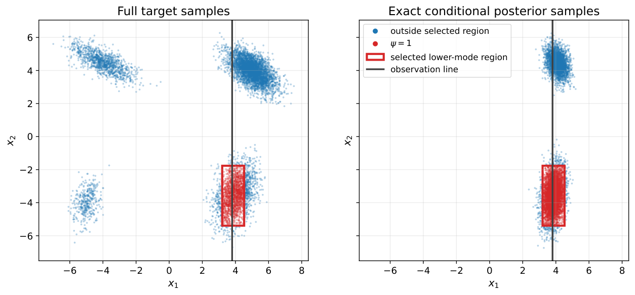
Refer to caption — Figure 1: Two-dimensional Gaussian-mixture benchmark. The red rectangle defines the event $\{\psi_{\mathcal{R}}=1\}$ used to evaluate the samplers. Left: samples from the original Gaussian mixture. Right: samples from the exact conditional posterior. Blue dots correspond to points outside the selected region, while red dots correspond to points inside it. The black vertical line indicates the observed value $y=3.8$ .

Figure 2 displays the two effects predicted by Theorem 3.11. In the left panel, for each method and particle count, we report the empirical $L_{2}$ error of between the method used and the oracle $\phi_{N}\!\left[\psi_{\mathcal{R}}\right]$ over independent SMC repetitions. The SMC sampler based on the exact reverse kernels has no proposal bias, and its empirical error decreases with a rate compatible with the Monte Carlo scale $M^{-1/2}$ . The oracle Euler kernels isolate the deterministic time-discretization bias, while the perturbed-score Euler kernels add a score-approximation bias. Accordingly, the corresponding curves initially decrease with $M$ , but eventually reach a non-vanishing large-particle plateau when the deterministic bias dominates the finite-particle error.

In the right panel, we isolate the propagation of a single local kernel perturbation. To make the effect visible, we use a larger particle count than in the particle-count experiment, so that the remaining Monte Carlo variability is small compared with the induced local-kernel bias. For each $\ell\in\{1,\ldots,N\}$ , we consider a hybrid sampler in which all mutation kernels are exact except the $\ell$ -th one:

Q_{m}^{(\ell)}:=\begin{cases}\overline{\mathsf{Q}}_{\ell}^{\theta},&m=\ell\,,\\ \mathsf{Q}_{m},&m\neq\ell\,.\end{cases}

Thus the local perturbation replaces the exact reverse kernel $\mathsf{Q}_{\ell}$ by an Euler kernel driven by a perturbed score. This single replacement contains both a time-discretization error and a local score-approximation error. We denote by $\phi_{N}^{(\ell)}$ the corresponding terminal distribution and estimate

\left|\phi_{N}^{(\ell)}[\psi_{\mathcal{R}}]-\phi_{N}\!\left[\psi_{\mathcal{R}}\right]\right|

as a function of the number of remaining steps $N-\ell$ . Perturbations introduced early in the sampling are attenuated strongly, consistently with the forward-smoothing forgetting factors $\rho_{\mathsf{G}}^{N-\ell}$ appearing in Theorem 3.11.

Figure 2: Illustration of the two terms in Theorem 3.11. Left: empirical

L_{2}

error as a function of the number of particles

M

, showing Monte Carlo decay and deterministic bias plateaus for approximate mutation kernels. Right: propagated effect of a single local kernel perturbation as a function of the number of remaining bridge steps, illustrating forward-smoothing forgetting. On the right panel, the left side corresponds to perturbations close to the data distribution

p_{0}

, while the right side corresponds to perturbations closer to the initial noised distribution

p_{T}

. Error bars show empirical standard errors across independent repetitions.

6 Discussion

This work provides a first perturbation analysis of Feynman–Kac particle systems with biased mutation kernels and specializes it to conditional sampling with score-based diffusion models. Although our bounds are explicit and non-asymptotic, the constants are not optimized. Deriving sharper constants would be important both theoretically and practically. In particular, more precise estimates of the forgetting constants would make it possible to adapt the training effort and the number of Monte Carlo particles to the stability properties of the underlying conditional sampler.

References

Cardoso et al., (2023) Cardoso, G., El Idrissi, Y. J., Le Corff, S., Moulines, E., and Olsson, J. (2023). State and parameter learning with paris particle gibbs. In International Conference on Machine Learning, pages 3625–3675. PMLR.
Cardoso et al., (2024) Cardoso, G., Janati El Idrissi, Y., Le Corff, S., and Moulines, E. (2024). Monte carlo guided denoising diffusion models for bayesian linear inverse problems. In International Conference on Learning Representations.
Chopin and Papaspiliopoulos, (2020) Chopin, N. and Papaspiliopoulos, O. (2020). An Introduction to Sequential Monte Carlo. Springer Series in Statistics. Springer.
Del Moral, (2004) Del Moral, P. (2004). Feynman-Kac Formulae: Genealogical and Interacting Particle Systems with Applications. Probability and Its Applications. Springer.
Del Moral et al., (2010) Del Moral, P., Doucet, A., and Singh, S. S. (2010). A backward particle interpretation of feynman-kac formulae. ESAIM: Mathematical Modelling and Numerical Analysis, 44(5):947–975.
Douc et al., (2018) Douc, R., Moulines, E., Priouret, P., and Soulier, P. (2018). Markov Chains. Springer Series in Operations Research and Financial Engineering. Springer, Cham.
Douc et al., (2004) Douc, R., Moulines, E., and Rosenthal, J. S. (2004). Quantitative bounds on convergence of time-inhomogeneous markov chains. Annals of Applied Probability, pages 1643–1665.
Douc et al., (2014) Douc, R., Moulines, E., and Stoffer, D. S. (2014). Nonlinear Time Series: Theory, Methods and Applications with R Examples. Chapman & Hall/CRC Texts in Statistical Science. CRC Press.
Dubarry and Le Corff, (2013) Dubarry, C. and Le Corff, S. (2013). Non-asymptotic deviation inequalities for smoothed additive functionals in nonlinear state-space models. Bernoulli, 19(5B):2222 – 2249.
Gloaguen et al., (2022) Gloaguen, P., Le Corff, S., and Olsson, J. (2022). A pseudo-marginal sequential monte carlo online smoothing algorithm. Bernoulli, 28(4):2606–2633.
Hairer and Mattingly, (2008) Hairer, M. and Mattingly, J. C. (2008). Yet another look at harris’ ergodic theorem for markov chains. arXiv preprint arXiv:0810.2777.
Haussmann and Pardoux, (1986) Haussmann, U. G. and Pardoux, E. (1986). Time reversal of diffusions. The Annals of Probability, 14(4):1188–1205.
Ho et al., (2020) Ho, J., Jain, A., and Abbeel, P. (2020). Denoising diffusion probabilistic models. In Advances in Neural Information Processing Systems (NeurIPS), pages 6840–6851.
Ho and Salimans, (2021) Ho, J. and Salimans, T. (2021). Classifier-free diffusion guidance. In NeurIPS 2021 Workshop on Deep Generative Models and Downstream Applications.
Meyn and Tweedie, (2009) Meyn, S. P. and Tweedie, R. L. (2009). Markov Chains and Stochastic Stability. Cambridge University Press, Cambridge, 2 edition.
Nazemi et al., (2024) Nazemi, A., Sepanj, M. H., Pellegrino, N., Czarnecki, C., and Fieguth, P. (2024). Particle-filtering-based latent diffusion for inverse problems.
Rombach et al., (2022) Rombach, R., Blattmann, A., Lorenz, D., Esser, P., and Ommer, B. (2022). High-resolution image synthesis with latent diffusion models. In Proceedings of the IEEE/CVF Conference on Computer Vision and Pattern Recognition (CVPR), pages 10684–10695.
Rudin, (1987) Rudin, W. (1987). Real and Complex Analysis. McGraw-Hill, Singapore.
Saharia et al., (2022) Saharia, C., Chan, W., Chang, H., Lee, C. A., Ho, J., Salimans, T., Fleet, D. J., and Norouzi, M. (2022). Palette: Image-to-image diffusion models. In ACM SIGGRAPH 2022 Conference Proceedings, New York, NY, USA. Association for Computing Machinery.
Sohl-Dickstein et al., (2015) Sohl-Dickstein, J., Weiss, E., Maheswaranathan, N., and Ganguli, S. (2015). Deep unsupervised learning using nonequilibrium thermodynamics. In Bach, F. and Blei, D., editors, Proceedings of the 32nd International Conference on Machine Learning, volume 37 of Proceedings of Machine Learning Research, pages 2256–2265, Lille, France. PMLR.
Song and Ermon, (2019) Song, Y. and Ermon, S. (2019). Generative modeling by estimating gradients of the data distribution. In Advances in Neural Information Processing Systems (NeurIPS), pages 11918–11930.
Song et al., (2021) Song, Y. W., Sohl-Dickstein, J., Kingma, D. P., Kumar, A., Ermon, S., and Poole, B. (2021). Score-based generative modeling through stochastic differential equations. In International Conference on Learning Representations.
Strasman et al., (2026) Strasman, S., Cardoso, G., Le Corff, S., Lemaire, V., and Ocello, A. (2026). On forgetting and stability of score-based generative models. arXiv preprint arXiv:2601.21868.
Vincent, (2011) Vincent, P. (2011). A connection between score matching and denoising autoencoders. Neural Computation, 23(7):1661–1674.
Whiteley, (2012) Whiteley, N. (2012). Sequential monte carlo samplers: error bounds and insensitivity to initial conditions. Stochastic Analysis and Applications, 30(5):774–798.
Wu et al., (2023) Wu, L., Trippe, B. L., Naesseth, C. A., Blei, D. M., and Cunningham, J. P. (2023). Practical and asymptotically exact conditional sampling in diffusion models. In Advances in Neural Information Processing Systems.

Notation	Meaning
$\{t_{k}\}_{k=0}^{N}$	Time grid
$\Delta_{k}$	Time step or integrated noise step between $t_{k}$ and $t_{k+1}$
$\mathsf{Q}_{k}$	Ideal mutation kernel from time $t_{k-1}$ to time $t_{k}$
$\mathsf{Q}_{k}^{\theta}$	Approximate mutation kernel from time $t_{k-1}$ to time $t_{k}$
$g_{k}$	Potential function at time $t_{k}$
$\tilde{g}_{k}$	Normalized potential, $\tilde{g}_{k}=g_{k}/\\|g_{k}\\|_{\infty}$
$\tau_{g}$	Tilting map by $g$ , $\tau_{g}(\nu)[\psi]=\nu[g\psi]/\nu[g]$
$\mathsf{K}_{k}$	Ideal unnormalized selection–mutation kernel, $\mathsf{K}_{k}=g_{k-1}\mathsf{Q}_{k}$
$\mathsf{K}_{k}^{\theta}$	Approximate unnormalized selection–mutation kernel, $\mathsf{K}_{k}^{\theta}=g_{k-1}\mathsf{Q}_{k}^{\theta}$
$\mathbb{F}_{k}$	Ideal normalized Feynman–Kac transform, $\mathbb{F}_{k}(\nu)=\nu\mathsf{K}_{k}/(\nu\mathsf{K}_{k}\mathds{1})$
$\mathbb{F}_{k}^{\theta}$	Approximate normalized Feynman–Kac transform, $\mathbb{F}_{k}^{\theta}(\nu)=\nu\mathsf{K}_{k}^{\theta}/(\nu\mathsf{K}_{k}^{\theta}\mathds{1})$
$\phi_{k}$	Ideal Feynman–Kac flow at time $t_{k}$
$\phi_{k}^{\theta}$	Approximate Feynman–Kac flow at time $t_{k}$
$\phi_{k}^{\theta,M}$	Empirical particle approximation of $\phi_{k}^{\theta}$
$\widetilde{\phi}_{k}^{\theta,M}$	Selected empirical measure after reweighting/resampling at time $t_{k}$
$\widetilde{\beta}_{k\|\ell}^{\theta}$	Normalized continuation function from time $k$ to terminal time $\ell$
$\mathsf{G}_{k\|\ell}^{\theta}$	Forward-smoothing kernel from time $k-1$ to time $k$ , associated with terminal time $\ell$
$\mathsf{G}_{k:\ell}^{\theta}$	Product of forward-smoothing kernels from time $k$ to time $\ell$
$V_{k\|N}^{\theta}$	Twisted Lyapunov function, $V/\widetilde{\beta}_{k\|N}^{\theta}$
$\Gamma_{\ell,N}$	Forward-smoothing stability coefficient from time $\ell$ to terminal time $N$
$\Lambda_{\ell,N}$	Normalization factor appearing in the deterministic kernel-bias bound
$\mathcal{E}_{k}^{\rm bias}$	Local one-step kernel-bias function at time $k$
$\mathcal{B}_{k}^{\rm bias}$	Integrated local bias under the selected exact filter
$\overline{\mathcal{B}}_{k}^{\rm bias}$	Effective local bias term used in the final total error bound
$\eta_{\ell}^{M,\theta}$	One-step predictive law before sampling at time $\ell$ in the particle system
$\mathcal{A}_{\ell,N}^{(p)}$	Monte Carlo normalization moment coefficient
$C_{\ell}^{\rm MC}$	Local Monte Carlo fluctuation constant
$w_{k}^{(i)}$	Normalized particle weight at time $t_{k}$
$\mathbf{X}_{k}^{\theta,(i)}$	Particle $i$ at time $t_{k}$
$\widetilde{\mathbf{X}}_{k}^{\theta,(i)}$	Selected particle $i$ after resampling at time $t_{k}$
$\mathcal{F}_{k}^{\theta}$	Particle filtration up to time $t_{k}$
$\widetilde{\mathcal{F}}_{k}^{\theta}$	Filtration after selection/resampling at time $t_{k}$

Table 1: Summary of the main notation.

Appendix A Forward smoothing kernel: properties and forgetting.

Proposition A.1 (Approximate tail factorization).

Let $0\leq k\leq m\leq N$ . For every probability measure $\nu\in\mathcal{P}(\mathbb{R}^{d})$ such that $0<\nu(\widetilde{\beta}_{k|m}^{\theta})<\infty$ , with $\widetilde{\beta}_{k|m}^{\theta}$ defined as in (9), we have

\displaystyle\left(\mathbb{F}_{m}^{\theta}\circ\cdots\circ\mathbb{F}_{k+1}^{\theta}\right)\left(\nu\right)

\displaystyle=\nu_{k|m}^{\theta}\mathsf{G}_{k+1|m}^{\theta}\cdots\mathsf{G}_{m|m}^{\theta}\,,\qquad\text{ with }\nu_{k|m}^{\theta}:=\frac{\widetilde{\beta}_{k|m}^{\theta}\nu}{\nu[\widetilde{\beta}_{k|m}^{\theta}]}\,.

(12)

Proof.

For $0\leq k<m\leq N$ , set

C_{k:m}:=\prod_{i=k}^{m-1}\left\|g_{i}\right\|_{\infty}\,.

Recall that

\displaystyle\left(\mathbb{F}_{m}^{\theta}\circ\cdots\circ\mathbb{F}_{k+1}^{\theta}\right)\left(\nu\right)=\frac{\nu\mathsf{K}_{k+1}^{\theta}\cdots\mathsf{K}_{m}^{\theta}}{\nu\mathsf{K}_{k+1}^{\theta}\cdots\mathsf{K}_{m}^{\theta}\mathds{1}}\,,

with the unnormalized kernels $\mathsf{K}_{\ell}^{\theta}$ , for $k+1\leq\ell\leq m$ , as in (2). We first show by induction on $m-k$ that, for every bounded measurable test function $\psi$ ,

\displaystyle\mathsf{K}_{k+1}^{\theta}\cdots\mathsf{K}_{m}^{\theta}\psi=C_{k:m}\widetilde{\beta}_{k|m}^{\theta}\mathsf{G}_{k+1|m}^{\theta}\cdots\mathsf{G}_{m|m}^{\theta}\psi\,.

(13)

First note that when $m=k+1$ ,

\displaystyle\widetilde{\beta}_{k|k+1}^{\theta}(\mathbf{x}_{k})=\tilde{g}_{k}(\mathbf{x}_{k})\,,\qquad\mathsf{G}_{k+1|k+1}^{\theta}=\mathsf{Q}_{k+1}^{\theta}\,,

and therefore,

\displaystyle\mathsf{K}_{k+1}^{\theta}\psi(\mathbf{x}_{k})=g_{k}(\mathbf{x}_{k})\mathsf{Q}_{k+1}^{\theta}\psi(\mathbf{x}_{k})=\left\|g_{k}\right\|_{\infty}\widetilde{\beta}_{k|k+1}^{\theta}(\mathbf{x}_{k})\mathsf{G}_{k+1|k+1}^{\theta}\psi(\mathbf{x}_{k})\,.

Then, assume that (13) holds for the pair $(k+1,m)$ , with $k+1<m$ , namely

\mathsf{K}_{k+2}^{\theta}\cdots\mathsf{K}_{m}^{\theta}\psi=C_{k+1:m}\widetilde{\beta}_{k+1|m}^{\theta}\mathsf{G}_{k+2|m}^{\theta}\cdots\mathsf{G}_{m|m}^{\theta}\psi\,.

Then, for any bounded measurable $\psi$ ,

	$\displaystyle\mathsf{K}_{k+1}^{\theta}\mathsf{K}_{k+2}^{\theta}\cdots\mathsf{K}_{m}^{\theta}\psi(\mathbf{x}_{k})$	$\displaystyle\quad=C_{k+1:m}\,g_{k}(\mathbf{x}_{k})\mathsf{Q}_{k+1}^{\theta}\left(\widetilde{\beta}_{k+1\|m}^{\theta}\mathsf{G}_{k+2\|m}^{\theta}\cdots\mathsf{G}_{m\|m}^{\theta}\psi\right)(\mathbf{x}_{k})$
		$\displaystyle\quad=C_{k:m}\,\tilde{g}_{k}(\mathbf{x}_{k})\mathsf{Q}_{k+1}^{\theta}\left(\widetilde{\beta}_{k+1\|m}^{\theta}\mathsf{G}_{k+2\|m}^{\theta}\cdots\mathsf{G}_{m\|m}^{\theta}\psi\right)(\mathbf{x}_{k})\,.$

By definition, the normalized continuation functions satisfy the recursion

\widetilde{\beta}_{k|m}^{\theta}(\mathbf{x}_{k})=\tilde{g}_{k}(\mathbf{x}_{k})\mathsf{Q}_{k+1}^{\theta}\widetilde{\beta}_{k+1|m}^{\theta}(\mathbf{x}_{k})\,,

so we obtain

\displaystyle\mathsf{K}_{k+1}^{\theta}\cdots\mathsf{K}_{m}^{\theta}\psi(\mathbf{x}_{k})

\displaystyle=C_{k:m}\widetilde{\beta}_{k|m}^{\theta}(\mathbf{x}_{k})\frac{\mathsf{Q}_{k+1}^{\theta}\left(\widetilde{\beta}_{k+1|m}^{\theta}\mathsf{G}_{k+2|m}^{\theta}\cdots\mathsf{G}_{m|m}^{\theta}\psi\right)(\mathbf{x}_{k})}{\mathsf{Q}_{k+1}^{\theta}\widetilde{\beta}_{k+1|m}^{\theta}(\mathbf{x}_{k})}\,.

By definition of the forward smoothing kernel (10),

		$\displaystyle\frac{\mathsf{Q}_{k+1}^{\theta}\left(\widetilde{\beta}_{k+1\|m}^{\theta}\mathsf{G}_{k+2\|m}^{\theta}\cdots\mathsf{G}_{m\|m}^{\theta}\psi\right)(\mathbf{x}_{k})}{\mathsf{Q}_{k+1}^{\theta}\widetilde{\beta}_{k+1\|m}^{\theta}(\mathbf{x}_{k})}$
		$\displaystyle=\frac{\int\widetilde{\beta}_{k+1\|m}^{\theta}(\mathbf{x}_{k+1})\left(\mathsf{G}_{k+2\|m}^{\theta}\cdots\mathsf{G}_{m\|m}^{\theta}\psi\right)(\mathbf{x}_{k+1})\mathsf{Q}_{k+1}^{\theta}(\mathbf{x}_{k},\mathrm{d}\mathbf{x}_{k+1})}{\mathsf{Q}_{k+1}^{\theta}\widetilde{\beta}_{k+1\|m}^{\theta}(\mathbf{x}_{k})}$
		$\displaystyle=\int\left(\mathsf{G}_{k+2\|m}^{\theta}\cdots\mathsf{G}_{m\|m}^{\theta}\psi\right)(\mathbf{x}_{k+1})\mathsf{G}_{k+1\|m}^{\theta}(\mathbf{x}_{k},\mathrm{d}\mathbf{x}_{k+1})$
		$\displaystyle=\mathsf{G}_{k+1\|m}^{\theta}\mathsf{G}_{k+2\|m}^{\theta}\cdots\mathsf{G}_{m\|m}^{\theta}\psi(\mathbf{x}_{k})\,.$

Therefore,

\displaystyle\mathsf{K}_{k+1}^{\theta}\cdots\mathsf{K}_{m}^{\theta}\psi(\mathbf{x}_{k})=C_{k:m}\widetilde{\beta}_{k|m}^{\theta}(\mathbf{x}_{k})\mathsf{G}_{k+1|m}^{\theta}\cdots\mathsf{G}_{m|m}^{\theta}\psi(\mathbf{x}_{k})\,,

which proves (13). Finally, applying (13) with $\psi$ and with $\mathds{1}$ , and using that each $\mathsf{G}_{\ell|m}^{\theta}$ is a Markov kernel, for $k+1\leq\ell\leq m$ , so that

\displaystyle\mathsf{G}_{k+1|m}^{\theta}\cdots\mathsf{G}_{m|m}^{\theta}\mathds{1}=\mathds{1}\,,

we get

	$\displaystyle\left(\mathbb{F}_{m}^{\theta}\circ\cdots\circ\mathbb{F}_{k+1}^{\theta}\right)(\nu)[\psi]$	$\displaystyle=\frac{\nu\mathsf{K}_{k+1}^{\theta}\cdots\mathsf{K}_{m}^{\theta}\psi}{\nu\mathsf{K}_{k+1}^{\theta}\cdots\mathsf{K}_{m}^{\theta}\mathds{1}}$
		$\displaystyle=\frac{C_{k:m}\nu\left[\widetilde{\beta}_{k\|m}^{\theta}\mathsf{G}_{k+1\|m}^{\theta}\cdots\mathsf{G}_{m\|m}^{\theta}\psi\right]}{C_{k:m}\nu\left[\widetilde{\beta}_{k\|m}^{\theta}\right]}$
		$\displaystyle=\frac{\nu\left[\widetilde{\beta}_{k\|m}^{\theta}\,\mathsf{G}_{k+1\|m}^{\theta}\cdots\mathsf{G}_{m\|m}^{\theta}\psi\right]}{\nu\left[\widetilde{\beta}_{k\|m}^{\theta}\right]}$
		$\displaystyle=\left(\nu_{k\|m}^{\theta}\mathsf{G}_{k+1\|m}^{\theta}\cdots\mathsf{G}_{m\|m}^{\theta}\right)\left[\psi\right]\,.$

which holds for every bounded measurable $\psi$ , and therefore proves (12). ∎

Remark A.2.

This factorization is purely algebraic and is not specific to the approximate Feynman–Kac model. It holds for any sequence of Markov kernels and their associated continuation functions and forward-smoothing kernels.

We now give conditions under which the forward smoothing kernels appearing in the factorization are themselves forgetting kernels, starting with a drift transfer condition.

Lemma A.3 (Forgetting transfer conditions).

Suppose that Assumptions 3.1-3.3 hold and define

V_{k|N}^{\theta}(\mathbf{x}):=\frac{V(\mathbf{x})}{\widetilde{\beta}_{k|N}^{\theta}(\mathbf{x})}\,,\qquad 0\leq k\leq N\,.

Then, for every $R>0$ , every $1\leq k\leq N$ , every $\mathbf{x}_{k-1}\in C_{R}$ , and every $A\in\mathcal{B}(\mathbb{R}^{d})$ ,

\mathsf{G}_{k|N}^{\theta}(\mathbf{x}_{k-1},A)\geq\varepsilon_{k}^{Q}(R)c_{k,R}^{Q}\nu_{k,R}^{\mathsf{G}}(A)\,,

(14)

where

\nu_{k,R}^{\mathsf{G}}(A):=\frac{\nu_{k,R}^{Q}\left[\widetilde{\beta}_{k|N}^{\theta}\mathds{1}_{A}\right]}{\nu_{k,R}^{Q}\left[\widetilde{\beta}_{k|N}^{\theta}\right]}\,.

Here the dependence of $\nu_{k,R}^{\mathsf{G}}$ on $N$ and $\theta$ is dropped. Moreover, for every $1\leq k\leq N$ , choose $R_{k}>0$ such that

R_{k}>\frac{K_{k}^{Q}}{1-\lambda_{k}^{Q}},

and define

\lambda_{k}^{\mathsf{G}}:=\lambda_{k}^{Q}+\frac{K_{k}^{Q}}{R_{k}}\in(0,1)\,,\qquad K_{k}^{\mathsf{G}}:=\frac{K_{k}^{Q}}{\varepsilon_{k}^{Q}(R_{k})c_{k,R_{k}}^{Q}}\,.

Then, for every $1\leq k\leq N$ and every $\mathbf{x}_{k-1}\in\mathbb{R}^{d}$ ,

\mathsf{G}_{k|N}^{\theta}V_{k|N}^{\theta}(\mathbf{x}_{k-1})\leq\lambda_{k}^{\mathsf{G}}V_{k-1|N}^{\theta}(\mathbf{x}_{k-1})+K_{k}^{\mathsf{G}}\mathds{1}_{C_{R_{k}}}(\mathbf{x}_{k-1})\,,

(15)

where $C_{R_{k}}=\{\mathbf{x}\in\mathbb{R}^{d}:V(\mathbf{x})\leq R_{k}\}$ .

Proof.

Since $0<\tilde{g}_{\ell}\leq 1$ for $0\leq\ell\leq N-1$ , we have

0<\widetilde{\beta}_{k|N}^{\theta}\leq 1\,,\qquad 0\leq k\leq N\,.

Therefore,

\mathsf{Q}_{k}^{\theta}\widetilde{\beta}_{k|N}^{\theta}(\mathbf{x}_{k-1})\leq 1\,.

Let $R>0$ , $\mathbf{x}_{k-1}\in C_{R}$ , and $A\in\mathcal{B}(\mathbb{R}^{d})$ . By the definition of $\mathsf{G}_{k|N}^{\theta}$ and the minorization condition,

	$\displaystyle\mathsf{G}_{k\|N}^{\theta}(\mathbf{x}_{k-1},A)$	$\displaystyle=\frac{\mathsf{Q}_{k}^{\theta}\left(\widetilde{\beta}_{k\|N}^{\theta}\mathds{1}_{A}\right)(\mathbf{x}_{k-1})}{\mathsf{Q}_{k}^{\theta}\widetilde{\beta}_{k\|N}^{\theta}(\mathbf{x}_{k-1})}$
		$\displaystyle\geq\mathsf{Q}_{k}^{\theta}\left(\widetilde{\beta}_{k\|N}^{\theta}\mathds{1}_{A}\right)(\mathbf{x}_{k-1})$
		$\displaystyle\geq\varepsilon_{k}^{Q}(R)\nu_{k,R}^{Q}\left[\widetilde{\beta}_{k\|N}^{\theta}\mathds{1}_{A}\right]\,.$

Moreover, using (11)

\nu_{k,R}^{Q}\left[\widetilde{\beta}_{k|N}^{\theta}\mathds{1}_{A}\right]=\nu_{k,R}^{Q}\left[\widetilde{\beta}_{k|N}^{\theta}\right]\nu_{k,R}^{\mathsf{G}}(A)=c_{k,R}^{Q}\nu_{k,R}^{\mathsf{G}}(A)\,.

Thus

\mathsf{G}_{k|N}^{\theta}(\mathbf{x}_{k-1},A)\geq\varepsilon^{Q}_{k}(R)c_{k,R}^{Q}\nu_{k,R}^{\mathsf{G}}(A)\,,

which proves (14).

For the drift condition, note that

\widetilde{\beta}_{k-1|N}^{\theta}=\tilde{g}_{k-1}\mathsf{Q}_{k}^{\theta}\widetilde{\beta}_{k|N}^{\theta}\leq\mathsf{Q}_{k}^{\theta}\widetilde{\beta}_{k|N}^{\theta}\,.

(16)

Hence,

\frac{V(\mathbf{x}_{k-1})}{\mathsf{Q}_{k}^{\theta}\widetilde{\beta}_{k|N}^{\theta}(\mathbf{x}_{k-1})}\leq\frac{V(\mathbf{x}_{k-1})}{\widetilde{\beta}_{k-1|N}^{\theta}(\mathbf{x}_{k-1})}=V_{k-1|N}^{\theta}(\mathbf{x}_{k-1})\,.

Using the drift condition in 3.1, we obtain

	$\displaystyle\mathsf{G}_{k\|N}^{\theta}V_{k\|N}^{\theta}(\mathbf{x}_{k-1})$	$\displaystyle=\int\frac{V(\mathbf{x}_{k})}{\widetilde{\beta}_{k\|N}^{\theta}(\mathbf{x}_{k})}\frac{\widetilde{\beta}_{k\|N}^{\theta}(\mathbf{x}_{k})\mathsf{Q}_{k}^{\theta}(\mathbf{x}_{k-1},\mathrm{d}\mathbf{x}_{k})}{\mathsf{Q}_{k}^{\theta}\widetilde{\beta}_{k\|N}^{\theta}(\mathbf{x}_{k-1})}$
		$\displaystyle=\frac{\mathsf{Q}_{k}^{\theta}V(\mathbf{x}_{k-1})}{\mathsf{Q}_{k}^{\theta}\widetilde{\beta}_{k\|N}^{\theta}(\mathbf{x}_{k-1})}$
		$\displaystyle\leq\lambda_{k}^{Q}V_{k-1\|N}^{\theta}(\mathbf{x}_{k-1})+\frac{K_{k}^{Q}}{\mathsf{Q}_{k}^{\theta}\widetilde{\beta}_{k\|N}^{\theta}(\mathbf{x}_{k-1})}\,.$

It remains to control the offset term. Fix $R_{k}>K_{k}^{Q}/(1-\lambda_{k}^{Q})$ . If $\mathbf{x}_{k-1}\notin C_{R_{k}}$ , then $V(\mathbf{x}_{k-1})>R_{k}$ , and

\frac{K_{k}^{Q}}{\mathsf{Q}_{k}^{\theta}\widetilde{\beta}_{k|N}^{\theta}(\mathbf{x}_{k-1})}=\frac{K_{k}^{Q}}{V(\mathbf{x}_{k-1})}\frac{V(\mathbf{x}_{k-1})}{\mathsf{Q}_{k}^{\theta}\widetilde{\beta}_{k|N}^{\theta}(\mathbf{x}_{k-1})}\leq\frac{K_{k}^{Q}}{R_{k}}V_{k-1|N}^{\theta}(\mathbf{x}_{k-1})\,,

where we used (16) in the last inequality. If $\mathbf{x}_{k-1}\in C_{R_{k}}$ , then the minorization condition (8) gives

\mathsf{Q}_{k}^{\theta}\widetilde{\beta}_{k|N}^{\theta}(\mathbf{x}_{k-1})\geq\varepsilon^{Q}_{k}(R_{k})\nu_{k,R_{k}}^{Q}\left[\widetilde{\beta}_{k|N}^{\theta}\right]=\varepsilon^{Q}_{k}(R_{k})c_{k,R_{k}}^{Q}\,.

Therefore,

\frac{K_{k}^{Q}}{\mathsf{Q}_{k}^{\theta}\widetilde{\beta}_{k|N}^{\theta}(\mathbf{x}_{k-1})}\leq\frac{K_{k}^{Q}}{\varepsilon^{Q}_{k}(R_{k})c_{k,R_{k}}^{Q}}\mathds{1}_{C_{R_{k}}}(\mathbf{x}_{k-1})+\frac{K_{k}^{Q}}{R_{k}}V_{k-1|N}^{\theta}(\mathbf{x}_{k-1})\,.

Combining this with the previous drift bound yields

\mathsf{G}_{k|N}^{\theta}V_{k|N}^{\theta}(\mathbf{x}_{k-1})\leq\left(\lambda_{k}^{Q}+\frac{K_{k}^{Q}}{R_{k}}\right)V_{k-1|N}^{\theta}(\mathbf{x}_{k-1})+\frac{K_{k}^{Q}}{\varepsilon^{Q}_{k}(R_{k})c_{k,R_{k}}^{Q}}\mathds{1}_{C_{R_{k}}}(\mathbf{x}_{k-1})\,.

By definition,

\lambda_{k}^{\mathsf{G}}=\lambda_{k}^{Q}+\frac{K_{k}^{Q}}{R_{k}}\,,\qquad K_{k}^{\mathsf{G}}=\frac{K_{k}^{Q}}{\varepsilon^{Q}_{k}(R_{k})c_{k,R_{k}}^{Q}}\,.

Since $R_{k}>K_{k}^{Q}/(1-\lambda_{k}^{Q})$ , we have $\lambda_{k}^{\mathsf{G}}\in(0,1)$ . This proves (15). ∎

Proposition A.4 (Bivariate conditions for the forward-smoothing kernels).

Suppose that Assumptions 3.1-3.3 hold and therefore that the conclusions of Lemma A.3 hold. For $0\leq k\leq N$ , define

F_{k|N}(\mathbf{x}):=1+\left(V_{k|N}^{\theta}(\mathbf{x})\right)\,,

and, for $(\mathbf{x},\mathbf{x}^{\prime})\in\mathbb{R}^{d}\times\mathbb{R}^{d}$ ,

\overline{F}_{k|N}(\mathbf{x},\mathbf{x}^{\prime}):=\frac{1}{2}\left[F_{k|N}(\mathbf{x})+F_{k|N}(\mathbf{x}^{\prime})\right]\,.

For $1\leq k\leq N$ , let $\lambda_{k}^{\mathsf{G}}\in(0,1)$ , $K_{k}^{\mathsf{G}}<\infty$ be the constants of Lemma A.3, choose

d_{k}>\frac{1-\lambda_{k}^{\mathsf{G}}+K_{k}^{\mathsf{G}}}{1-\lambda_{k}^{\mathsf{G}}}\,,

(17)

and define

\overline{C}_{k}:=\left\{(\mathbf{x},\mathbf{x}^{\prime}):\overline{F}_{k-1|N}(\mathbf{x},\mathbf{x}^{\prime})\leq d_{k}\right\}\,.

Let

L_{k}:=2d_{k}-1\,.

Define

\overline{\varepsilon}_{k}:=\frac{\varepsilon^{Q}_{k}(L_{k})c_{k,L_{k}}^{Q}}{2}\,,

(18)

\overline{\lambda}_{k}:=\lambda_{k}^{\mathsf{G}}+\frac{1-\lambda_{k}^{\mathsf{G}}+K_{k}^{\mathsf{G}}}{d_{k}}\in(0,1)\,,

(19)

and

\overline{b}_{k}:=\frac{\lambda_{k}^{\mathsf{G}}d_{k}+1-\lambda_{k}^{\mathsf{G}}+K_{k}^{\mathsf{G}}}{1-\overline{\varepsilon}_{k}}\,.

(20)

Then the kernels $(\mathsf{G}_{k|N}^{\theta})_{1\leq k\leq N}$ satisfy the time-inhomogeneous conditions NS1 and NS2 of Douc et al., 2004. More precisely,

\mathsf{G}_{k|N}^{\theta}(\mathbf{x},\cdot)\wedge\mathsf{G}_{k|N}^{\theta}(\mathbf{x}^{\prime},\cdot)\geq\overline{\varepsilon}_{k}\nu_{k,L_{k}}^{\mathsf{G}}(\cdot),\qquad(\mathbf{x},\mathbf{x}^{\prime})\in\overline{C}_{k}\,.

and there exists a bivariate kernel $\mathsf{G}_{k|N}^{\theta,*}$ such that

\mathsf{G}_{k|N}^{\theta,*}\overline{F}_{k|N}(\mathbf{x},\mathbf{x}^{\prime})\leq\overline{\lambda}_{k}\overline{F}_{k-1|N}(\mathbf{x},\mathbf{x}^{\prime})+\overline{b}_{k}\mathds{1}_{\overline{C}_{k}}(\mathbf{x},\mathbf{x}^{\prime})\,.

(21)

Proof.

We first prove NS1. By the minorization bound obtained in Lemma A.3, for every $R>0$ , every $\mathbf{x}\in C_{R}$ , and every $A\in\mathcal{B}(\mathbb{R}^{d})$ ,

\mathsf{G}_{k|N}^{\theta}(\mathbf{x},A)\geq\varepsilon^{Q}_{k}(R)c_{k,R}^{Q}\nu_{k,R}^{\mathsf{G}}(A)\,.

Let $(\mathbf{x},\mathbf{x}^{\prime})\in\overline{C}_{k}$ . By definition of $\overline{C}_{k}$ ,

\overline{F}_{k-1|N}(\mathbf{x},\mathbf{x}^{\prime})=\frac{1}{2}\left[F_{k-1|N}(\mathbf{x})+F_{k-1|N}(\mathbf{x}^{\prime})\right]\leq d_{k}\,.

Since both terms are nonnegative, this implies

F_{k-1|N}(\mathbf{x})\leq 2d_{k}\,,\qquad F_{k-1|N}(\mathbf{x}^{\prime})\leq 2d_{k}\,.

Therefore,

V_{k-1|N}^{\theta}(\mathbf{x})\leq 2d_{k}-1=L_{k}\,,\qquad V_{k-1|N}^{\theta}(\mathbf{x}^{\prime})\leq L_{k}\,.

Moreover, since $0<\widetilde{\beta}_{k-1|N}^{\theta}\leq 1$ ,

V(\mathbf{x})\leq L_{k}\,,\qquad V(\mathbf{x}^{\prime})\leq L_{k}\,,

that is $\mathbf{x},\mathbf{x}^{\prime}\in C_{L_{k}}$ with

C_{L_{k}}=\left\{\mathbf{z}\in\mathbb{R}^{d}:V(\mathbf{z})\leq L_{k}\right\}\,.

Applying the one-step minorization (14) with $R=L_{k}$ , we obtain

\mathsf{G}_{k|N}^{\theta}(\mathbf{x},\cdot)\geq\varepsilon^{Q}_{k}(L_{k})c_{k,L_{k}}^{Q}\nu_{k,L_{k}}^{\mathsf{G}}(\cdot)\,,

and

\mathsf{G}_{k|N}^{\theta}(\mathbf{x}^{\prime},\cdot)\geq\varepsilon^{Q}_{k}(L_{k})c_{k,L_{k}}^{Q}\nu_{k,L_{k}}^{\mathsf{G}}(\cdot)\,.

Hence,

\mathsf{G}_{k|N}^{\theta}(\mathbf{x},\cdot)\wedge\mathsf{G}_{k|N}^{\theta}(\mathbf{x}^{\prime},\cdot)\geq\overline{\varepsilon}_{k}\nu_{k,L_{k}}^{\mathsf{G}}(\cdot),

where $\overline{\varepsilon}_{k}=\tfrac{1}{2}\varepsilon^{Q}_{k}(L_{k})c_{k,L_{k}}^{Q}$ . This proves NS1.

We now prove NS2. Using the one-step drift bound (15),

\mathsf{G}_{k|N}^{\theta}V_{k|N}^{\theta}(\mathbf{x})\leq\lambda_{k}^{\mathsf{G}}V_{k-1|N}^{\theta}(\mathbf{x})+K_{k}^{\mathsf{G}}\mathds{1}_{C_{R_{k}}}(\mathbf{x})\,.

Therefore,

\mathsf{G}_{k|N}^{\theta}\left(V_{k|N}^{\theta}\right)(\mathbf{x})\leq\lambda_{k}^{\mathsf{G}}\left(V_{k-1|N}^{\theta}(\mathbf{x})\right)+K_{k}^{\mathsf{G}}\mathds{1}_{C_{R_{k}}}(\mathbf{x})\,.

We get,

	$\displaystyle\mathsf{G}_{k\|N}^{\theta}F_{k\|N}(\mathbf{x})$	$\displaystyle=1+\mathsf{G}_{k\|N}^{\theta}\left(V_{k\|N}^{\theta}\right)(\mathbf{x})$
		$\displaystyle\leq 1+\lambda_{k}^{\mathsf{G}}\left(V_{k-1\|N}^{\theta}(\mathbf{x})\right)+K_{k}^{\mathsf{G}}$
		$\displaystyle=\lambda_{k}^{\mathsf{G}}F_{k-1\|N}(\mathbf{x})+1-\lambda_{k}^{\mathsf{G}}+K_{k}^{\mathsf{G}}\,.$

Define the bivariate kernel $\mathsf{G}_{k|N}^{\theta,*}$ on $\mathbb{R}^{d}\times\mathbb{R}^{d}$ by

		$\displaystyle\mathsf{G}_{k\|N}^{\theta,*}((\mathbf{x},\mathbf{x}^{\prime}),\mathrm{d}\mathbf{z},\mathrm{d}\mathbf{z}^{\prime}):=$
		$\displaystyle\begin{cases}\displaystyle\mathsf{G}_{k\|N}^{\theta}(\mathbf{x},\mathrm{d}\mathbf{z})\mathsf{G}_{k\|N}^{\theta}(\mathbf{x}^{\prime},\mathrm{d}\mathbf{z}^{\prime}),&(\mathbf{x},\mathbf{x}^{\prime})\notin\overline{C}_{k}\,,\\[9.47217pt] \displaystyle\frac{\left(\mathsf{G}_{k\|N}^{\theta}(\mathbf{x},\mathrm{d}\mathbf{z})-\overline{\varepsilon}_{k}\nu_{k,L_{k}}^{\mathsf{G}}(\mathrm{d}\mathbf{z})\right)\left(\mathsf{G}_{k\|N}^{\theta}(\mathbf{x}^{\prime},\mathrm{d}\mathbf{z}^{\prime})-\overline{\varepsilon}_{k}\nu_{k,L_{k}}^{\mathsf{G}}(\mathrm{d}\mathbf{z}^{\prime})\right)}{(1-\overline{\varepsilon}_{k})^{2}}&(\mathbf{x},\mathbf{x}^{\prime})\in\overline{C}_{k}\,.\\[9.47217pt] \end{cases}$

If $(\mathbf{x},\mathbf{x}^{\prime})\notin\overline{C}_{k}$ , then by definition of $\mathsf{G}_{k|N}^{\theta,*}$ ,

	$\displaystyle\mathsf{G}_{k\|N}^{\theta,*}\overline{F}_{k\|N}(\mathbf{x},\mathbf{x}^{\prime})$	$\displaystyle=\frac{1}{2}\mathsf{G}_{k\|N}^{\theta}F_{k\|N}(\mathbf{x})+\frac{1}{2}\mathsf{G}_{k\|N}^{\theta}F_{k\|N}(\mathbf{x}^{\prime})$
		$\displaystyle\leq\lambda_{k}^{\mathsf{G}}\overline{F}_{k-1\|N}(\mathbf{x},\mathbf{x}^{\prime})+1-\lambda_{k}^{\mathsf{G}}+K_{k}^{\mathsf{G}}\,.$

Since $(\mathbf{x},\mathbf{x}^{\prime})\notin\overline{C}_{k}$ , we have $\overline{F}_{k-1|N}(\mathbf{x},\mathbf{x}^{\prime})>d_{k}$ , and therefore,

1-\lambda_{k}^{\mathsf{G}}+K_{k}^{\mathsf{G}}\leq\frac{1-\lambda_{k}^{\mathsf{G}}+K_{k}^{\mathsf{G}}}{d_{k}}\overline{F}_{k-1|N}(\mathbf{x},\mathbf{x}^{\prime})\,.

Hence,

\mathsf{G}_{k|N}^{\theta,*}\overline{F}_{k|N}(\mathbf{x},\mathbf{x}^{\prime})\leq\overline{\lambda}_{k}\overline{F}_{k-1|N}(\mathbf{x},\mathbf{x}^{\prime})\,,

where $\overline{\lambda}_{k}\in(0,1)$ is defined in (19).

If $(\mathbf{x},\mathbf{x}^{\prime})\in\overline{C}_{k}$ , as $0<\overline{\varepsilon}_{k}<1$ , and by definition of $\mathsf{G}_{k|N}^{\theta,*}$ ,

	$\displaystyle\mathsf{G}_{k\|N}^{\theta,*}\overline{F}_{k\|N}(\mathbf{x},\mathbf{x}^{\prime})$	$\displaystyle=\frac{\mathsf{G}_{k\|N}^{\theta}F_{k\|N}(\mathbf{x})+\mathsf{G}_{k\|N}^{\theta}F_{k\|N}(\mathbf{x}^{\prime})-2\overline{\varepsilon}_{k}\nu_{k,L_{k}}^{\mathsf{G}}[F_{k\|N}]}{2(1-\overline{\varepsilon}_{k})}$
		$\displaystyle\leq\frac{\mathsf{G}_{k\|N}^{\theta}F_{k\|N}(\mathbf{x})+\mathsf{G}_{k\|N}^{\theta}F_{k\|N}(\mathbf{x}^{\prime})}{2(1-\overline{\varepsilon}_{k})}$
		$\displaystyle\leq\frac{\lambda_{k}^{\mathsf{G}}\overline{F}_{k-1\|N}(\mathbf{x},\mathbf{x}^{\prime})+1-\lambda_{k}^{\mathsf{G}}+K_{k}^{\mathsf{G}}}{1-\overline{\varepsilon}_{k}}\,.$

Since $(\mathbf{x},\mathbf{x}^{\prime})\in\overline{C}_{k}$ , we have $\overline{F}_{k-1|N}(\mathbf{x},\mathbf{x}^{\prime})\leq d_{k}$ . Thus

\mathsf{G}_{k|N}^{\theta,*}\overline{F}_{k|N}(\mathbf{x},\mathbf{x}^{\prime})\leq\frac{\lambda_{k}^{\mathsf{G}}d_{k}+1-\lambda_{k}^{\mathsf{G}}+K_{k}^{\mathsf{G}}}{1-\overline{\varepsilon}_{k}}=\overline{b}_{k}\,,

(22)

where we used (20). Combining the two cases, we obtain (21). This proves NS2. ∎

Corollary A.5.

Suppose that Assumptions 3.1-3.3 hold and that the conditions of Proposition A.4 hold. Then, for every $0\leq\ell\leq N$ , there exists a finite constant $\Gamma_{\ell,N}<\infty$ , depending only on

(\overline{\varepsilon}_{k},\overline{\lambda}_{k},\overline{b}_{k})_{\ell+1\leq k\leq N}\,,

such that, for all probability measures $\mu_{1},\mu_{2}$ satisfying

\mu_{1}\left[1+V_{\ell|N}^{\theta}\right]+\mu_{2}\left[1+V_{\ell|N}^{\theta}\right]<\infty\,,

we have

\left\|\mu_{1}\mathsf{G}_{\ell:N}^{\theta}-\mu_{2}\mathsf{G}_{\ell:N}^{\theta}\right\|_{V}\leq\Gamma_{\ell,N}\left\{\mu_{1}\left[1+V_{\ell|N}^{\theta}\right]+\mu_{2}\left[1+V_{\ell|N}^{\theta}\right]\right\}\,,

where $\Gamma_{\ell,N}$ is defined in (25). Moreover, for every finite signed measure $\eta$ such that

\eta(\mathbb{R}^{d})=0\,,\qquad|\eta|\left[1+V_{\ell|N}^{\theta}\right]<\infty\,,

we have

\left\|\eta\mathsf{G}_{\ell:N}^{\theta}\right\|_{V}\leq\Gamma_{\ell,N}|\eta|\left[1+V_{\ell|N}^{\theta}\right]=\Gamma_{\ell,N}\left\|\eta\right\|_{V_{\ell|N}^{\theta}}\,.

(23)

Proof.

We have,

\left\|\mu_{1}\mathsf{G}_{\ell:N}^{\theta}-\mu_{2}\mathsf{G}_{\ell:N}^{\theta}\right\|_{V}=\left\|\mu_{1}\mathsf{G}_{\ell+1|N}^{\theta}\cdots\mathsf{G}_{N|N}^{\theta}-\mu_{2}\mathsf{G}_{\ell+1|N}^{\theta}\cdots\mathsf{G}_{N|N}^{\theta}\right\|_{V}

The case $\ell=N$ follows from

\mathsf{G}_{N:N}^{\theta}=\operatorname{Id}\,,\qquad V_{N|N}^{\theta}=V\,.

Recall that, for $0\leq k\leq N$ ,

F_{k|N}(\mathbf{x}):=1+\left(V_{k|N}^{\theta}(\mathbf{x})\right)\,.

Now, let $0\leq\ell<N$ , in the notation of Douc et al., 2004, we use the correspondence

\lambda_{i-1}=\overline{\lambda}_{\ell+i}\,,\qquad b_{i-1}=\overline{b}_{\ell+i}\,,\qquad\overline{V}_{0}=\overline{F}_{\ell|N},\qquad 1\leq i\leq N-\ell\,.

For $j\in\{1,\cdots,N-\ell\}$ , define

(1-\overline{\varepsilon})_{j,\ell:N}:=\max_{\ell+1\leq r_{1}<\cdots<r_{j}\leq N}\prod_{q=1}^{j}\left(1-\overline{\varepsilon}_{r_{q}}\right)\,,\qquad\overline{B}_{j,\ell:N}:=\max_{\ell+1\leq r_{1}<\cdots<r_{j}\leq N}\prod_{q=1}^{j}\overline{B}_{r_{q}}\,,

with $\overline{B}_{0,\ell:N}:=1$ and

\overline{B}_{r}:=1\vee\frac{(1-\overline{\varepsilon}_{r})\overline{b}_{r}}{\overline{\lambda}_{r}}\,.

(24)

Note that $\overline{B}_{r}$ is an upper bound to equation (26) in Douc et al., 2004 given by (22). Applying Douc et al., 2004, for every $1\leq j\leq N-\ell+1$ ,

		$\displaystyle\left\\|\mu_{1}\mathsf{G}_{\ell+1\|N}^{\theta}\cdots\mathsf{G}_{N\|N}^{\theta}-\mu_{2}\mathsf{G}_{\ell+1\|N}^{\theta}\cdots\mathsf{G}_{N\|N}^{\theta}\right\\|_{V}$
		$\displaystyle\quad\leq 2(1-\overline{\varepsilon})_{j,\ell:N}D_{\ell,N}(\mu_{1},\mu_{2})\mathds{1}_{\{j\leq N-\ell\}}+2\left(\prod_{r=\ell+1}^{N}\overline{\lambda}_{r}\right)\overline{B}_{j-1,\ell:N}(\mu_{1}\otimes\mu_{2})[\overline{F}_{\ell\|N}]\,.$

where

D_{\ell,N}(\mu_{1},\mu_{2}):=\left(\prod_{r=\ell+1}^{N}\overline{\lambda}_{r}\right)(\mu_{1}\otimes\mu_{2})\left[\overline{F}_{\ell|N}\right]+\sum_{s=\ell+1}^{N}\left(\prod_{r=s+1}^{N}\overline{\lambda}_{r}\right)\overline{b}_{s}\,.

Since

(\mu_{1}\otimes\mu_{2})[\overline{F}_{\ell|N}]=\frac{1}{2}\left\{\mu_{1}[F_{\ell|N}]+\mu_{2}[F_{\ell|N}]\right\}\,,

and since $F_{\ell|N}\geq 1$ , we have

\mu_{1}[F_{\ell|N}]+\mu_{2}[F_{\ell|N}]\geq 2\,.

Therefore,

	$\displaystyle 2D_{\ell,N}(\mu_{1},\mu_{2})$	$\displaystyle=\left(\prod_{r=\ell+1}^{N}\overline{\lambda}_{r}\right)\left\{\mu_{1}[F_{\ell\|N}]+\mu_{2}[F_{\ell\|N}]\right\}+2\sum_{s=\ell+1}^{N}\left(\prod_{r=s+1}^{N}\overline{\lambda}_{r}\right)\overline{b}_{s}$
		$\displaystyle\leq\left[\left(\prod_{r=\ell+1}^{N}\overline{\lambda}_{r}\right)+\sum_{s=\ell+1}^{N}\left(\prod_{r=s+1}^{N}\overline{\lambda}_{r}\right)\overline{b}_{s}\right]\left\{\mu_{1}[F_{\ell\|N}]+\mu_{2}[F_{\ell\|N}]\right\}\,.$

Thus, for probability measures $\mu_{1},\mu_{2}$ and for every $1\leq j\leq N-\ell+1$ ,

		$\displaystyle\left\\|\mu_{1}\mathsf{G}_{\ell:N}^{\theta}-\mu_{2}\mathsf{G}_{\ell:N}^{\theta}\right\\|_{V}\leq\Bigg[(1-\overline{\varepsilon})_{j,\ell:N}\left\{\left(\prod_{r=\ell+1}^{N}\overline{\lambda}_{r}\right)+\sum_{s=\ell+1}^{N}\left(\prod_{r=s+1}^{N}\overline{\lambda}_{r}\right)\overline{b}_{s}\right\}\mathds{1}_{\{j\leq N-\ell\}}$
		$\displaystyle\qquad\qquad\qquad\qquad\qquad\qquad\qquad\qquad+\left(\prod_{r=\ell+1}^{N}\overline{\lambda}_{r}\right)\overline{B}_{j-1,\ell:N}\Bigg]\left\{\mu_{1}[F_{\ell\|N}]+\mu_{2}[F_{\ell\|N}]\right\}\,.$

Taking the infimum over $1\leq j\leq N-\ell+1$ , we obtain

\left\|\mu_{1}\mathsf{G}_{\ell:N}^{\theta}-\mu_{2}\mathsf{G}_{\ell:N}^{\theta}\right\|_{V}\leq\Gamma_{\ell,N}\left\{\mu_{1}[F_{\ell|N}]+\mu_{2}[F_{\ell|N}]\right\}\,,

where

\Gamma_{\ell,N}:=\inf_{1\leq j\leq N-\ell+1}\Bigg[(1-\overline{\varepsilon})_{j,\ell:N}\left\{\left(\prod_{r=\ell+1}^{N}\overline{\lambda}_{r}\right)+\sum_{s=\ell+1}^{N}\left(\prod_{r=s+1}^{N}\overline{\lambda}_{r}\right)\overline{b}_{s}\right\}\mathds{1}_{\{j\leq N-\ell\}}\\ +\left(\prod_{r=\ell+1}^{N}\overline{\lambda}_{r}\right)\overline{B}_{j-1,\ell:N}\Bigg]\,,

(25)

with the convention that $\Gamma_{N,N}:=1$ .

It remains to prove the signed-measure extension. Let $\eta$ be a finite signed measure such that $\eta(\mathbb{R}^{d})=0$ , and let

\eta=\eta^{+}-\eta^{-}

be its Jordan decomposition. If $\eta=0$ , the result is immediate. Otherwise, since $\eta(\mathbb{R}^{d})=0$ , we have

s:=\eta^{+}(\mathbb{R}^{d})=\eta^{-}(\mathbb{R}^{d})>0\,.

Define the probability measures

\pi^{+}:=\frac{\eta^{+}}{s}\,,\qquad\pi^{-}:=\frac{\eta^{-}}{s}\,.

Then $\eta=s(\pi^{+}-\pi^{-})$ . Applying the first part of the corollary to $\pi^{+}$ and $\pi^{-}$ , we obtain

	$\displaystyle\left\\|\eta\mathsf{G}_{\ell:N}^{\theta}\right\\|_{V}$	$\displaystyle=s\left\\|\pi^{+}\mathsf{G}_{\ell:N}^{\theta}-\pi^{-}\mathsf{G}_{\ell:N}^{\theta}\right\\|_{V}$
		$\displaystyle\leq s\Gamma_{\ell,N}\left\{\pi^{+}[1+V_{\ell\|N}^{\theta}]+\pi^{-}[1+V_{\ell\|N}^{\theta}]\right\}$
		$\displaystyle=\Gamma_{\ell,N}\|\eta\|\left[1+V_{\ell\|N}^{\theta}\right]\,.$

which proves (23). ∎

Corollary A.6 (Geometric forgetting under uniform constants).

Suppose that Assumptions 3.1-3.3 hold, so that the conclusions of Proposition A.4 hold. Suppose moreover that there exist constants

\varepsilon_{\star}>0\,,\qquad\lambda_{\star}\in(0,1)\,,\qquad b_{\star}<\infty\,,\qquad B_{\star}\in[1,\infty)\,,

such that, for every $1\leq k\leq N$ ,

\overline{\varepsilon}_{k}\geq\varepsilon_{\star}\,,\qquad\overline{\lambda}_{k}\leq\lambda_{\star}\,,\qquad\overline{b}_{k}\leq b_{\star}\,,\qquad\overline{B}_{k}\leq B_{\star}\,.

Then there exist constants $M_{\mathsf{G}}<\infty$ and $\rho_{\mathsf{G}}\in(0,1)$ , independent of $N$ and $\ell$ , such that for every $N\geq 1$ and $0\leq\ell\leq N$ ,

\Gamma_{\ell,N}\leq M_{\mathsf{G}}\rho_{\mathsf{G}}^{N-\ell}\,,

where

\rho_{\mathsf{G}}:=\max\left\{(1-\varepsilon_{\star})^{\delta},\lambda_{\star}B_{\star}^{\delta}\right\}\,.

and

M_{\mathsf{G}}:=2+\frac{b_{\star}}{1-\lambda_{\star}}\,.

Proof.

The case $\ell=N$ is immediate. Indeed, by convention,

\mathsf{G}_{N:N}^{\theta}=\operatorname{Id}

and therefore,

\left\|\mu_{1}\mathsf{G}_{N:N}^{\theta}-\mu_{2}\mathsf{G}_{N:N}^{\theta}\right\|_{V}=\left\|\mu_{1}-\mu_{2}\right\|_{V}\,.

Suppose, now that, $N-\ell\geq 1$ , using the uniform bounds,

\prod_{r=\ell+1}^{N}\overline{\lambda}_{r}\leq\lambda_{\star}^{N-\ell}\,,\qquad\sum_{s=\ell+1}^{N}\left(\prod_{r=s+1}^{N}\overline{\lambda}_{r}\right)\overline{b}_{s}\leq b_{\star}\sum_{q=0}^{N-\ell-1}\lambda_{\star}^{q}\leq\frac{b_{\star}}{1-\lambda_{\star}}\,.

Moreover,

(1-\overline{\varepsilon})_{j,\ell:N}\leq(1-\varepsilon_{\star})^{j}\,,\qquad\overline{B}_{j-1,\ell:N}\leq B_{\star}^{j-1}\,.

Hence, we have

\Gamma_{\ell,N}\leq\inf_{1\leq j\leq N-\ell+1}\left\{\left(\lambda_{\star}^{N-\ell}+\frac{b_{\star}}{1-\lambda_{\star}}\right)(1-\varepsilon_{\star})^{j}\mathds{1}_{\{j\leq N-\ell\}}+\lambda_{\star}^{N-\ell}B_{\star}^{j-1}\right\}\,.

We want to find a choice of $j$ that would yield a geometric decay of length $N-\ell$ . Since $B_{\star}\in[1,\infty)$ and $\lambda_{\star}\in(0,1)$ , choose $\delta\in(0,1)$ such that

\lambda_{\star}B_{\star}^{\delta}<1.

Since $N-\ell\geq 1$ and $\delta\in(0,1)$ , let $j_{\delta}:=\left\lceil\delta(N-\ell)\right\rceil$ and we have

1\leq j_{\delta}<N-\ell+1\,.

Thus,

\Gamma_{\ell,N}\leq\left(\lambda_{\star}^{N-\ell}+\frac{b_{\star}}{1-\lambda_{\star}}\right)(1-\varepsilon_{\star})^{j_{\delta}}+\lambda_{\star}^{N-\ell}B_{\star}^{j_{\delta}-1}\,.

Because $j_{\delta}\geq\delta(N-\ell)$ ,

(1-\varepsilon_{\star})^{j_{\delta}}\leq\left((1-\varepsilon_{\star})^{\delta}\right)^{N-\ell}\,.

Because $j_{\delta}-1\leq\delta(N-\ell)$ and $B_{\star}\geq 1$ ,

\lambda_{\star}^{N-\ell}B_{\star}^{j_{\delta}-1}\leq\left(\lambda_{\star}B_{\star}^{\delta}\right)^{N-\ell}\,.

Therefore,

\Gamma_{\ell,N}\leq\left(\lambda_{\star}^{N-\ell}+\frac{b_{\star}}{1-\lambda_{\star}}\right)\left((1-\varepsilon_{\star})^{\delta}\right)^{N-\ell}+\left(\lambda_{\star}B_{\star}^{\delta}\right)^{N-\ell}\,.

By construction, $\rho_{\mathsf{G}}\in(0,1)$ , and therefore,

\Gamma_{\ell,N}\leq\left(\lambda_{\star}^{N-\ell}+\frac{b_{\star}}{1-\lambda_{\star}}+1\right)\rho_{\mathsf{G}}^{N-\ell}=M_{\mathsf{G}}\rho_{\mathsf{G}}^{N-\ell}\,,

which concludes the proof. ∎

Lemma A.7 (Sufficient condition for uniform time control).

Suppose 3.6 holds. Then there exist constants

\varepsilon_{\star}>0\,,\qquad\lambda_{\star}\in(0,1)\,,\qquad b_{\star}<\infty\,,\qquad B_{\star}\in[1,\infty)\,,

independent of $N$ , such that, for every $N\geq 1$ and every $1\leq k\leq N$ ,

\overline{\varepsilon}_{k}\geq\varepsilon_{\star}\,,\qquad\overline{\lambda}_{k}\leq\lambda_{\star}\,,\qquad\overline{b}_{k}\leq b_{\star}\,,\qquad\overline{B}_{k}\leq B_{\star}\,,

where $\overline{\varepsilon}_{k}$ , $\overline{\lambda}_{k}$ , $\overline{b}_{k}$ and $\overline{B}_{k}$ are defined in Proposition A.4.

Proof.

Let $N\geq 1$ and $1\leq k\leq N$ . All constants constructed below are independent of $N$ and $k$ . In Lemma A.3, take $R_{k}=R_{\star}$ . Then, the transferred drift constants satisfy

\lambda_{k}^{\mathsf{G}}=\lambda_{k}^{Q}+\frac{K_{k}^{Q}}{R_{\star}}\leq\lambda_{Q}+\frac{K_{Q}}{R_{\star}}\eqqcolon\lambda_{\mathsf{G},\star}<1\,.

Moreover, by 3.6,

K_{k}^{\mathsf{G}}=\frac{K_{k}^{Q}}{\varepsilon_{k}^{Q}(R_{\star})c_{k,R_{\star}}^{Q}}\leq\frac{K_{Q}}{\eta_{R_{\star}}}\eqqcolon K_{\mathsf{G},\star}<\infty\,.

Choose

d_{k}:=2\frac{1-\lambda_{k}^{\mathsf{G}}+K_{k}^{\mathsf{G}}}{1-\lambda_{k}^{\mathsf{G}}}\,,

(26)

and note that such choice satisfies (17). It follows that,

d_{k}=2+\frac{2K_{k}^{\mathsf{G}}}{1-\lambda_{k}^{\mathsf{G}}}\leq 2+\frac{2K_{\mathsf{G},\star}}{1-\lambda_{\mathsf{G},\star}}\eqqcolon d_{\star}<\infty.

Since $L_{k}=2d_{k}-1$ , we obtain

L_{k}\leq 2d_{\star}-1=3+\frac{4K_{\mathsf{G},\star}}{1-\lambda_{\mathsf{G},\star}}=L_{\star}\,.

Hence $C_{L_{k}}\subseteq C_{L_{\star}}$ . Therefore, in the minorization step of Proposition A.4, we may use the radius $L_{\star}$ uniformly in $k$ and set

\overline{\varepsilon}_{k}:=\frac{1}{2}\varepsilon_{k}^{Q}(L_{\star})c_{k,L_{\star}}^{Q}.

By 3.6,

\overline{\varepsilon}_{k}\geq\frac{\eta_{L_{\star}}}{2}\eqqcolon\varepsilon_{\star}>0\,.

Furthermore, using (19) and (26)

\overline{\lambda}_{k}=\frac{1+\lambda_{k}^{\mathsf{G}}}{2}\leq\frac{1+\lambda_{\mathsf{G},\star}}{2}\eqqcolon\lambda_{\star}<1\,,

and using (20)

\overline{b}_{k}=\frac{\lambda_{k}^{\mathsf{G}}d_{k}+1-\lambda_{k}^{\mathsf{G}}+K_{k}^{\mathsf{G}}}{1-\overline{\varepsilon}_{k}}\leq 2\left(\lambda_{\mathsf{G},\star}d_{\star}+1+K_{\mathsf{G},\star}\right)\,,

where we used to bound the denominator that since $\varepsilon_{k}^{Q}(L_{\star})\leq 1$ and $0<c_{k,L_{\star}}^{Q}\leq 1$ ,

\overline{\varepsilon}_{k}=\frac{1}{2}\varepsilon_{k}^{Q}(L_{\star})c_{k,L_{\star}}^{Q}\leq\frac{1}{2}\,.

Finally, using (24) and since $\overline{\lambda}_{k}=\frac{1+\lambda_{k}^{\mathsf{G}}}{2}\geq 1/2$ ,

\overline{B}_{k}=1\vee\frac{(1-\overline{\varepsilon}_{k})\overline{b}_{k}}{\overline{\lambda}_{k}}\leq 1\vee 2\overline{b}_{k}\leq 1\vee 2b_{\star}\eqqcolon B_{\star}<\infty\,,

which concludes the proof. ∎

Appendix B Kernel bias: proofs

Proposition B.1 (Kernel bias error decomposition).

For every $N\geq 2$ ,

	$\displaystyle\phi_{N}-\phi_{N}^{\theta}$	$\displaystyle=\left(\mu_{0\|N}-\mu_{0\|N}^{\theta}\right)\mathsf{G}_{1\|N}^{\theta}\cdots\mathsf{G}_{N\|N}^{\theta}$
		$\displaystyle+\sum_{\ell=1}^{N-1}\left(\mu_{\ell\|N}-\mu_{\ell\|N}^{\theta}\right)\mathsf{G}_{\ell+1\|N}^{\theta}\cdots\mathsf{G}_{N\|N}^{\theta}+\left(\mathbb{F}_{N}(\phi_{N-1})-\mathbb{F}_{N}^{\theta}(\phi_{N-1})\right)\,,$

where for $1\leq\ell\leq N-1$ ,

\mu_{\ell|N}:=\frac{\widetilde{\beta}_{\ell|N}^{\theta}\mathbb{F}_{\ell}(\phi_{\ell-1})}{\mathbb{F}_{\ell}(\phi_{\ell-1})[\widetilde{\beta}_{\ell|N}^{\theta}]}\,,\qquad\mu_{\ell|N}^{\theta}:=\frac{\widetilde{\beta}_{\ell|N}^{\theta}\mathbb{F}_{\ell}^{\theta}(\phi_{\ell-1})}{\mathbb{F}_{\ell}^{\theta}(\phi_{\ell-1})[\widetilde{\beta}_{\ell|N}^{\theta}]}\,,

and

\mu_{0|N}:=\frac{\widetilde{\beta}_{0|N}^{\theta}\phi_{0}}{\phi_{0}\!\left[\widetilde{\beta}_{0|N}^{\theta}\right]}\,,\qquad\mu_{0|N}^{\theta}:=\frac{\widetilde{\beta}_{0|N}^{\theta}\phi_{0}^{\theta}}{\phi_{0}^{\theta}\!\left[\widetilde{\beta}_{0|N}^{\theta}\right]}\,.

Equivalently,

\displaystyle\phi_{N}-\phi_{N}^{\theta}=\sum_{\ell=0}^{N}\left(\mu_{\ell|N}-\mu_{\ell|N}^{\theta}\right)\mathsf{G}_{\ell:N}^{\theta}\,,

(27)

where $\mathsf{G}_{N:N}^{\theta}=\operatorname{Id}$ , and

\mu_{N|N}:=\mathbb{F}_{N}(\phi_{N-1})\,,\qquad\mu_{N|N}^{\theta}:=\mathbb{F}_{N}^{\theta}(\phi_{N-1})\,.

Proof.

We write

\phi_{N}=\left(\mathbb{F}_{N}\circ\cdots\circ\mathbb{F}_{1}\right)(\phi_{0}),\qquad\phi_{N}^{\theta}=\left(\mathbb{F}_{N}^{\theta}\circ\cdots\circ\mathbb{F}_{1}^{\theta}\right)(\phi_{0}^{\theta})\,.

A standard telescoping argument yields for any $N\geq 2$ ,

	$\displaystyle\phi_{N}-\phi_{N}^{\theta}$	$\displaystyle=\left(\mathbb{F}_{N}^{\theta}\circ\cdots\circ\mathbb{F}_{1}^{\theta}\right)(\phi_{0})-\left(\mathbb{F}_{N}^{\theta}\circ\cdots\circ\mathbb{F}_{1}^{\theta}\right)(\phi_{0}^{\theta})$
		$\displaystyle\qquad+\sum_{\ell=1}^{N-1}\Bigg\{\left(\mathbb{F}_{N}^{\theta}\circ\cdots\circ\mathbb{F}_{\ell+1}^{\theta}\right)\left(\phi_{\ell}\right)-\left(\mathbb{F}_{N}^{\theta}\circ\cdots\circ\mathbb{F}_{\ell+1}^{\theta}\right)\left(\mathbb{F}_{\ell}^{\theta}\left(\phi_{\ell-1}\right)\right)\Bigg\}$
		$\displaystyle\qquad+\mathbb{F}_{N}(\phi_{N-1})-\mathbb{F}_{N}^{\theta}(\phi_{N-1})\,.$

Then, applying Proposition A.1 finishes the proof. ∎

Lemma B.2.

Suppose that Assumptions 3.1, 3.2, 3.8 hold. Then, for every $1\leq k\leq N$ ,

\phi_{k}\!\left[V\right]<\infty\,,\qquad\mathbb{F}_{k}(\phi_{k-1})[V]<\infty\,,\qquad\mathbb{F}_{k}^{\theta}(\phi_{k-1})[V]<\infty\,.

Proof.

We prove the moment bounds by induction. The base case $\phi_{0}\!\left[V\right]<\infty$ is part of 3.8. Assume that $\phi_{k-1}\!\left[V\right]<\infty$ . Since $g_{k-1}$ is positive and bounded above by 3.2,

\tau_{g_{k-1}}(\phi_{k-1})[V]=\frac{\phi_{k-1}\!\left[g_{k-1}V\right]}{\phi_{k-1}\!\left[g_{k-1}\right]}<\infty\,.

Using 3.1,

\mathbb{F}_{k}^{\theta}(\phi_{k-1})[V]\leq\lambda_{k}^{Q}\tau_{g_{k-1}}(\phi_{k-1})[V]+K_{k}^{Q}<\infty\,.

Moreover, since $V\leq 1+V$ , and using 3.8

\mathsf{Q}_{k}V(\mathbf{x})\leq\mathsf{Q}_{k}^{\theta}V(\mathbf{x})+h\mathcal{E}_{k}^{\rm bias}(\mathbf{x})\,.

Therefore, using 3.8 again

	$\displaystyle\mathbb{F}_{k}(\phi_{k-1})[V]$	$\displaystyle=\tau_{g_{k-1}}(\phi_{k-1})\mathsf{Q}_{k}V$
		$\displaystyle\leq\tau_{g_{k-1}}(\phi_{k-1})\mathsf{Q}_{k}^{\theta}V+h\tau_{g_{k-1}}(\phi_{k-1})[\mathcal{E}_{k}^{\rm bias}]$
		$\displaystyle<\infty\,,$

where the last term is finite by 3.8. Since $\phi_{k}=\mathbb{F}_{k}(\phi_{k-1})$ , this proves the induction. ∎

Lemma B.3 (Kernel bias bound under forward-smoothing forgetting).

Suppose that Assumptions 3.1, 3.2, 3.3, and 3.8 hold. Define, for $1\leq\ell\leq N-1$

\Lambda_{\ell,N}:=\frac{1+\mu_{\ell|N}^{\theta}\!\left[F_{\ell|N}^{\theta}\right]}{\mathbb{F}_{\ell}(\phi_{\ell-1})\left[\widetilde{\beta}_{\ell|N}^{\theta}\right]}\,,

and

\Lambda_{0,N}:=\frac{1+\mu_{0|N}^{\theta}\!\left[F_{0|N}^{\theta}\right]}{\phi_{0}\left[\widetilde{\beta}_{0|N}^{\theta}\right]}\,,\qquad\Lambda_{N,N}:=1\,.

Then, for every $N\geq 2$ ,

	$\displaystyle\left\\|\phi_{N}-\phi_{N}^{\theta}\right\\|_{V}$	$\displaystyle\leq\Gamma_{0,N}\Lambda_{0,N}\left\\|\phi_{0}-\phi_{0}^{\theta}\right\\|_{V}+\sum_{\ell=1}^{N}\Gamma_{\ell,N}\Lambda_{\ell,N}\left\\|\mathbb{F}_{\ell}(\phi_{\ell-1})-\mathbb{F}_{\ell}^{\theta}(\phi_{\ell-1})\right\\|_{V}$
		$\displaystyle\leq\Gamma_{0,N}\Lambda_{0,N}\mathcal{B}_{0}^{\rm bias}+h\sum_{\ell=1}^{N}\Gamma_{\ell,N}\Lambda_{\ell,N}\mathcal{B}_{\ell}^{\rm bias}\,,$		(28)

with for $0\leq\ell\leq N$ , $\Gamma_{\ell,N}$ defined as in Corollary A.5 and $\Lambda_{\ell,N}<\infty$ .

Proof.

By Proposition B.1,

\phi_{N}-\phi_{N}^{\theta}=\sum_{\ell=0}^{N}\left(\mu_{\ell|N}-\mu_{\ell|N}^{\theta}\right)\mathsf{G}_{\ell:N}^{\theta}\,.

Using the triangle inequality and Corollary A.5, we get

\left\|\phi_{N}-\phi_{N}^{\theta}\right\|_{V}\leq\sum_{\ell=0}^{N}\Gamma_{\ell,N}\left\|\mu_{\ell|N}-\mu_{\ell|N}^{\theta}\right\|_{V_{\ell|N}^{\theta}}\,.

Recall that for $\mathbf{x}\in\mathbb{R}^{d}$ ,

F_{\ell|N}^{\theta}(\mathbf{x})=1+V_{\ell|N}^{\theta}(\mathbf{x})=1+\frac{V(\mathbf{x})}{\widetilde{\beta}_{\ell|N}^{\theta}(\mathbf{x})}\,,\qquad 0\leq\ell\leq N\,.

For $0\leq\ell\leq N-1$ , we use the following estimate. Let $\mu,\nu$ be probability measures such that $\mu[\widetilde{\beta}_{\ell|N}^{\theta}]>0$ and $\nu[\widetilde{\beta}_{\ell|N}^{\theta}]>0$ . Then

\displaystyle\left\|\frac{\widetilde{\beta}_{\ell|N}^{\theta}\mu}{\mu[\widetilde{\beta}_{\ell|N}^{\theta}]}-\frac{\widetilde{\beta}_{\ell|N}^{\theta}\nu}{\nu[\widetilde{\beta}_{\ell|N}^{\theta}]}\right\|_{V_{\ell|N}^{\theta}}\leq\frac{1+\left(\frac{\widetilde{\beta}_{\ell|N}^{\theta}\nu}{\nu[\widetilde{\beta}_{\ell|N}^{\theta}]}\right)[F_{\ell|N}^{\theta}]}{\mu[\widetilde{\beta}_{\ell|N}^{\theta}]}\left\|\mu-\nu\right\|_{V}\,.

(29)

Indeed, for every measurable $\psi$ such that $|\psi|\leq F_{\ell|N}^{\theta}$ ,

	$\displaystyle\left\|\frac{\mu[\widetilde{\beta}_{\ell\|N}^{\theta}\psi]}{\mu[\widetilde{\beta}_{\ell\|N}^{\theta}]}-\frac{\nu[\widetilde{\beta}_{\ell\|N}^{\theta}\psi]}{\nu[\widetilde{\beta}_{\ell\|N}^{\theta}]}\right\|$	$\displaystyle\leq\frac{\|\mu-\nu\|[\widetilde{\beta}_{\ell\|N}^{\theta}F_{\ell\|N}^{\theta}]}{\mu[\widetilde{\beta}_{\ell\|N}^{\theta}]}+\frac{\nu[\widetilde{\beta}_{\ell\|N}^{\theta}F_{\ell\|N}^{\theta}]}{\nu[\widetilde{\beta}_{\ell\|N}^{\theta}]}\frac{\|\mu-\nu\|[\widetilde{\beta}_{\ell\|N}^{\theta}]}{\mu[\widetilde{\beta}_{\ell\|N}^{\theta}]}$
		$\displaystyle\leq\frac{1+\left(\frac{\widetilde{\beta}_{\ell\|N}^{\theta}\nu}{\nu[\widetilde{\beta}_{\ell\|N}^{\theta}]}\right)\left[F_{\ell\|N}^{\theta}\right]}{\mu[\widetilde{\beta}_{\ell\|N}^{\theta}]}\|\mu-\nu\|[\widetilde{\beta}_{\ell\|N}^{\theta}F_{\ell\|N}^{\theta}]\,,$

where we used in the last inequality that $F_{\ell|N}^{\theta}\geq\mathds{1}$ , and therefore $|\mu-\nu|[\widetilde{\beta}_{\ell|N}^{\theta}]\leq|\mu-\nu|[\widetilde{\beta}_{\ell|N}^{\theta}F_{\ell|N}^{\theta}]$ . Also, since

\widetilde{\beta}_{\ell|N}^{\theta}F_{\ell|N}^{\theta}=\widetilde{\beta}_{\ell|N}^{\theta}+V\leq 1+V\,,

we obtain (29). Applying (29) with

\mu=\phi_{0}\,,\qquad\nu=\phi_{0}^{\theta}\,,

gives

\left\|\mu_{0|N}-\mu_{0|N}^{\theta}\right\|_{V_{0|N}^{\theta}}\leq\Lambda_{0,N}\left\|\phi_{0}-\phi_{0}^{\theta}\right\|_{V}\,,

It remains to use 3.8. The initial term satisfies

\left\|\phi_{0}-\phi_{0}^{\theta}\right\|_{V}\leq\mathcal{B}_{0}^{\rm bias}\,.

Similarly, for $1\leq\ell\leq N-1$ , applying (29) with

\mu=\mathbb{F}_{\ell}(\phi_{\ell-1})\,,\qquad\nu=\mathbb{F}_{\ell}^{\theta}(\phi_{\ell-1})\,,

gives

\left\|\mu_{\ell|N}-\mu_{\ell|N}^{\theta}\right\|_{V_{\ell|N}^{\theta}}\leq\Lambda_{\ell,N}\left\|\mathbb{F}_{\ell}(\phi_{\ell-1})-\mathbb{F}_{\ell}^{\theta}(\phi_{\ell-1})\right\|_{V}\,.

Moreover, recall that

\mathbb{F}_{k}(\phi_{k-1})=\tau_{g_{k-1}}(\phi_{k-1})\mathsf{Q}_{k}\,,\qquad\mathbb{F}_{k}^{\theta}(\phi_{k-1})=\tau_{g_{k-1}}(\phi_{k-1})\mathsf{Q}_{k}^{\theta}\,.

Hence, for every measurable $\psi$ such that $|\psi|\leq 1+V$ ,

	$\displaystyle\left\|\mathbb{F}_{k}(\phi_{k-1})[\psi]-\mathbb{F}_{k}^{\theta}(\phi_{k-1})[\psi]\right\|$	$\displaystyle=\left\|\int\left(\mathsf{Q}_{k}\psi(\mathbf{x})-\mathsf{Q}_{k}^{\theta}\psi(\mathbf{x})\right)\tau_{g_{k-1}}(\phi_{k-1})(\mathrm{d}\mathbf{x})\right\|$
		$\displaystyle\leq\int\left\\|\delta_{\mathbf{x}}\mathsf{Q}_{k}-\delta_{\mathbf{x}}\mathsf{Q}_{k}^{\theta}\right\\|_{V}\tau_{g_{k-1}}(\phi_{k-1})(\mathrm{d}\mathbf{x})$
		$\displaystyle\leq h\int\mathcal{E}_{k}^{\rm bias}(\mathbf{x})\tau_{g_{k-1}}(\phi_{k-1})(\mathrm{d}\mathbf{x})$
		$\displaystyle=h\tau_{g_{k-1}}(\phi_{k-1})[\mathcal{E}_{k}^{\rm bias}]\,.$

Taking the supremum over all $\psi$ such that $|\psi|\leq 1+V$ yields

\left\|\mathbb{F}_{k}(\phi_{k-1})-\mathbb{F}_{k}^{\theta}(\phi_{k-1})\right\|_{V}\leq h\left(\tau_{g_{k-1}}(\phi_{k-1})[\mathcal{E}_{k}^{\rm bias}]\right)\,.

Finally, for $\ell=N$ ,

\widetilde{\beta}_{N|N}^{\theta}=\mathds{1}\,,\qquad\mathsf{G}_{N:N}^{\theta}=\operatorname{Id}\,,\qquad\Lambda_{N,N}:=1\,,

and therefore

\left\|\mu_{N|N}-\mu_{N|N}^{\theta}\right\|_{V}=\left\|\mathbb{F}_{N}(\phi_{N-1})-\mathbb{F}_{N}^{\theta}(\phi_{N-1})\right\|_{V}\,.

It remains to prove the finiteness of $\Lambda_{\ell,N}$ . Since $0<\widetilde{\beta}_{\ell|N}^{\theta}\leq 1$ , for any probability measure $\mu$

0<\mu[\widetilde{\beta}_{\ell|N}^{\theta}]\leq 1\,,

and

\widetilde{\beta}_{\ell|N}^{\theta}F_{\ell|N}^{\theta}=\widetilde{\beta}_{\ell|N}^{\theta}+V\leq 1+V\,.

Hence, for $\ell=0$ , using 3.2 and 3.8,

\mu_{0|N}^{\theta}[F_{0|N}^{\theta}]=\frac{\phi_{0}^{\theta}\!\left[\widetilde{\beta}_{0|N}^{\theta}F_{0|N}^{\theta}\right]}{\phi_{0}^{\theta}\!\left[\widetilde{\beta}_{0|N}^{\theta}\right]}\leq\frac{1+\phi_{0}^{\theta}\!\left[V\right]}{\phi_{0}^{\theta}\!\left[\widetilde{\beta}_{0|N}^{\theta}\right]}<\infty\,.

For $1\leq\ell\leq N-1$ , the same argument holds with Lemma B.2,

\mu_{\ell|N}^{\theta}[F_{\ell|N}^{\theta}]=\frac{\mathbb{F}_{\ell}^{\theta}(\phi_{\ell-1})[\widetilde{\beta}_{\ell|N}^{\theta}F_{\ell|N}^{\theta}]}{\mathbb{F}_{\ell}^{\theta}(\phi_{\ell-1})[\widetilde{\beta}_{\ell|N}^{\theta}]}\leq\frac{1+\mathbb{F}_{\ell}^{\theta}(\phi_{\ell-1})[V]}{\mathbb{F}_{\ell}^{\theta}(\phi_{\ell-1})[\widetilde{\beta}_{\ell|N}^{\theta}]}<\infty\,.

Finally, $\Lambda_{N,N}=1$ , which concludes the proof. ∎

Appendix C Monte Carlo error: proofs

The proof follows the standard local-error propagation strategy for Feynman–Kac particle systems; see, for example, Del Moral, 2004 and Whiteley, 2012.

For $0\leq\ell\leq N$ , define the future normalized approximate Feynman–Kac map

\mathbb{F}_{\ell:N}^{\theta}:=\mathbb{F}_{N}^{\theta}\circ\cdots\circ\mathbb{F}_{\ell+1}^{\theta}\,,\qquad\mathbb{F}_{N:N}^{\theta}:=\operatorname{Id}\,.

Thus, for every probability measure $\nu$ ,

\mathbb{F}_{\ell:N}^{\theta}(\nu)=\left(\mathbb{F}_{N}^{\theta}\circ\cdots\circ\mathbb{F}_{\ell+1}^{\theta}\right)(\nu)\,.

Selected and propagated empirical measures.

At time $k-1$ , considering $M$ particles, let

\mathcal{F}_{k-1}^{\theta}:=\sigma\left(\mathbf{X}_{\ell}^{\theta,(i)},\,1\leq i\leq M,\,0\leq\ell\leq k-1\right)\,.

Given $\phi_{k-1}^{\theta,M}$ , the selection step draws

\widetilde{\mathbf{X}}_{k-1}^{\theta,(1)},\ldots,\widetilde{\mathbf{X}}_{k-1}^{\theta,(M)}\mid\mathcal{F}_{k-1}^{\theta}\overset{\mathrm{i.i.d.}}{\sim}\tau_{g_{k-1}}(\phi_{k-1}^{\theta,M})\,.

We define

\widetilde{\phi}_{k-1}^{\theta,M}:=\frac{1}{M}\sum_{i=1}^{M}\delta_{\widetilde{\mathbf{X}}_{k-1}^{\theta,(i)}}\,.

Let

\widetilde{\mathcal{F}}_{k-1}^{\theta}:=\sigma\left(\mathcal{F}_{k-1}^{\theta},\widetilde{\mathbf{X}}_{k-1}^{\theta,(1)},\ldots,\widetilde{\mathbf{X}}_{k-1}^{\theta,(M)}\right)\,.

The mutation step draws, conditionally independently given $\widetilde{\mathcal{F}}_{k-1}^{\theta}$ ,

\mathbf{X}_{k}^{\theta,(i)}\mid\widetilde{\mathcal{F}}_{k-1}^{\theta}\sim\mathsf{Q}_{k}^{\theta}(\widetilde{\mathbf{X}}_{k-1}^{\theta,(i)},\mathrm{d}\mathbf{x})\,,\qquad i=1,\ldots,M\,.

We define

\phi_{k}^{\theta,M}:=\frac{1}{M}\sum_{i=1}^{M}\delta_{\mathbf{X}_{k}^{\theta,(i)}}\,.

Consequently, for every bounded measurable function $\psi$ ,

\mathbb{E}\left[\phi_{k}^{\theta,M}\!\left[\psi\right]\middle|\mathcal{F}_{k-1}^{\theta}\right]=\tau_{g_{k-1}}(\phi_{k-1}^{\theta,M})\mathsf{Q}_{k}^{\theta}\left[\psi\right]=\mathbb{F}_{k}^{\theta}(\phi_{k-1}^{\theta,M})[\psi].

Local selection and mutation errors.

For every bounded measurable test function $\psi$ , define

\phi_{k}^{\theta,M}\!\left[\psi\right]-\mathbb{F}_{k}^{\theta}(\phi_{k-1}^{\theta,M})[\psi]=M_{k}^{M}\!\left[\psi\right]+S_{k}^{M}\!\left[\psi\right]\,,

where

M_{k}^{M}\!\left[\psi\right]:=\phi_{k}^{\theta,M}\!\left[\psi\right]-\frac{1}{M}\sum_{i=1}^{M}\mathsf{Q}_{k}^{\theta}\psi(\widetilde{\mathbf{X}}_{k-1}^{\theta,(i)})\,,

is the mutation error and

S_{k}^{M}\!\left[\psi\right]:=\frac{1}{M}\sum_{i=1}^{M}\mathsf{Q}_{k}^{\theta}\psi(\widetilde{\mathbf{X}}_{k-1}^{\theta,(i)})-\left(\tau_{g_{k-1}}(\phi_{k-1}^{\theta,M})\mathsf{Q}_{k}^{\theta}\right)[\psi]\,,

is the selection error. Then

\mathbb{E}[M_{k}^{M}\!\left[\psi\right]\mid\widetilde{\mathcal{F}}_{k-1}]=0\,,\qquad\mathbb{E}[S_{k}^{M}\!\left[\psi\right]\mid\mathcal{F}_{k-1}]=0\,.

Local $L_{p}$ control.

We now quantify the size of the local empirical errors introduced at each selection and mutation step. Since the final estimates are stated in a $V$ -weighted norm, we use the corresponding dual weighted supremum norm. For a measurable function $\psi:\mathbb{R}^{d}\to\mathbb{R}$ , define

\|\psi\|_{V,\infty}:=\sup_{\mathbf{x}\in\mathbb{R}^{d}}\frac{|\psi(\mathbf{x})|}{1+V(\mathbf{x})}\,.

Lemma C.1.

Let $q\geq 2$ and suppose that 3.9 holds. Then there exists a constant $B_{q}<\infty$ , depending only on $q$ , such that for every measurable $\psi:\mathbb{R}^{d}\to\mathbb{R}$ with $\|\psi\|_{V,\infty}<\infty$ ,

\left\|(\phi_{0}^{\theta,M}-\phi_{0}^{\theta})[\psi]\right\|_{L_{q}}\leq\frac{C_{0}^{(q)}}{\sqrt{M}}\|\psi\|_{V,\infty}\,,

(30)

and, for every $1\leq k\leq N$ ,

\left\|\phi_{k}^{\theta,M}\!\left[\psi\right]-\left(\mathbb{F}_{k}^{\theta}(\phi_{k-1}^{\theta,M})\right)[\psi]\right\|_{L_{q}}\leq\frac{C_{k}^{S,(q)}+C_{k}^{M,(q)}}{\sqrt{M}}\|\psi\|_{V,\infty}\,,

(31)

where

C_{0}^{(q)}:=2B_{q}\phi_{0}^{\theta}\!\left[(1+V)^{q}\right]^{1/q}\,,

C_{k}^{S,(q)}:=2B_{q}\left(\sup_{M\geq 1}\mathbb{E}\left[\tau_{g_{k-1}}(\phi_{k-1}^{\theta,M})[\mathsf{Q}_{k}^{\theta}(1+V)^{q}]\right]\right)^{1/q}\,,

and

C_{k}^{M,(q)}:=2B_{q}\left(\sup_{M\geq 1}\mathbb{E}\left[\widetilde{\phi}_{k-1}^{\theta,M}\!\left[\mathsf{Q}_{k}^{\theta}(1+V)^{q}\right]\right]\right)^{1/q}\,.

Proof.

The proof is an application of Lemma 7.7.3 (Chapter 7.3: Inequalities for independent Random Variables) in Del Moral, 2004.

Initial empirical error. By construction, the initial particles $\mathbf{X}_{0}^{\theta,(1)},\ldots,\mathbf{X}_{0}^{\theta,(M)}$ are i.i.d. with common law $\phi_{0}^{\theta}$ . Define

U_{i}:=\psi(\mathbf{X}_{0}^{\theta,(i)})-\phi_{0}^{\theta}\!\left[\psi\right],\qquad i=1,\ldots,M\,.

Then the variables $U_{1},\ldots,U_{M}$ are i.i.d. and centered, and

(\phi_{0}^{\theta,M}-\phi_{0}^{\theta})[\psi]=\frac{1}{M}\sum_{i=1}^{M}U_{i}\,.

Therefore, by Marcinkiewicz–Zygmund inequality,

\left\|(\phi_{0}^{\theta,M}-\phi_{0}^{\theta})[\psi]\right\|_{L_{q}}\leq\frac{B_{q}}{M}\left\|\left(\sum_{i=1}^{M}|U_{i}|^{2}\right)^{1/2}\right\|_{L_{q}}\,.

Since $q/2\geq 1$ , Jensen’s inequality yields

\left(\sum_{i=1}^{M}|U_{i}|^{2}\right)^{q/2}\leq M^{\frac{q}{2}-1}\sum_{i=1}^{M}|U_{i}|^{q}\,.

Hence

\left\|(\phi_{0}^{\theta,M}-\phi_{0}^{\theta})[\psi]\right\|_{L_{q}}\leq\frac{B_{q}}{\sqrt{M}}\left(\frac{1}{M}\sum_{i=1}^{M}\mathbb{E}[|U_{i}|^{q}]\right)^{1/q}\,.

Using $|a-b|^{q}\leq 2^{q-1}(|a|^{q}+|b|^{q})$ and Jensen’s inequality,

\displaystyle\mathbb{E}[|U_{i}|^{q}]

\displaystyle\leq 2^{q-1}\left(\mathbb{E}[|\psi(\mathbf{X}_{0}^{\theta,(i)})|^{q}]+|\phi_{0}^{\theta}\!\left[\psi\right]|^{q}\right)\leq 2^{q}\phi_{0}^{\theta}\!\left[|\psi|^{q}\right]\,.

Since $|\psi(\mathbf{x})|\leq\left\|\psi\right\|_{V,\infty}(1+V(\mathbf{x}))$ , we get

\phi_{0}^{\theta}\!\left[|\psi|^{q}\right]\leq\left\|\psi\right\|_{V,\infty}^{q}\phi_{0}^{\theta}\left[(1+V)^{q}\right]\,.

Combining the last displays proves (30).

Local selection error. By definition,

S_{k}^{M}\!\left[\psi\right]=\frac{1}{M}\sum_{i=1}^{M}\mathsf{Q}_{k}^{\theta}\psi(\widetilde{\mathbf{X}}^{\theta,(i)}_{k-1})-\tau_{g_{k-1}}(\phi_{k-1}^{\theta,M})\mathsf{Q}_{k}^{\theta}{\psi}\,.

Conditionally on $\mathcal{F}^{\theta}_{k-1}$ , the selected particles $\widetilde{\mathbf{X}}^{\theta,(1)}_{k-1},\ldots,\widetilde{\mathbf{X}}^{\theta,(M)}_{k-1}$ are i.i.d. with common law $\tau_{g_{k-1}}(\phi_{k-1}^{\theta,M})$ . Hence the variables

Y_{i}:=\mathsf{Q}_{k}^{\theta}\psi(\widetilde{\mathbf{X}}^{\theta,(i)}_{k-1})-\tau_{g_{k-1}}(\phi_{k-1}^{\theta,M})\mathsf{Q}_{k}^{\theta}{\psi}\,,\qquad i=1,\ldots,M\,,

are conditionally i.i.d. and centered. Therefore, by Marcinkiewicz-Zygmund inequality, there exists $B_{q}$ depending only on $q$ such that,

\displaystyle\left\|S_{k}^{M}\!\left[\psi\right]\right\|_{L_{q}(.|\mathcal{F}^{\theta}_{k-1})}

\displaystyle=\frac{1}{M}\left\|\sum_{i=1}^{M}Y_{i}\right\|_{L_{q}(.|\mathcal{F}_{k-1}^{\theta})}\leq\frac{B_{q}}{M}\left\|\left(\sum_{i=1}^{M}|Y_{i}|^{2}\right)^{1/2}\right\|_{L_{q}(.|\mathcal{F}^{\theta}_{k-1})}

where $L_{q}(.|\mathcal{F}^{\theta}_{k-1})$ means the $L_{q}$ norms is taken conditional on $\mathcal{F}^{\theta}_{k-1}$ . Since $q/2\geq 1$ , the map $x\mapsto x^{q/2}$ is convex. Hence, by Jensen,

\left(\sum_{i=1}^{M}|Y_{i}|^{2}\right)^{q/2}\leq M^{\frac{q}{2}-1}\sum_{i=1}^{M}|Y_{i}|^{q}\,,

Hence

\left\|S_{k}^{M}\!\left[\psi\right]\right\|_{L_{q}(.|\mathcal{F}^{\theta}_{k-1})}\leq\frac{B_{q}}{\sqrt{M}}\left(\frac{1}{M}\sum_{i=1}^{M}\mathbb{E}\left[|Y_{i}|^{q}\middle|\mathcal{F}^{\theta}_{k-1}\right]\right)^{1/q}\,.

Using $|a-b|^{q}\leq 2^{q-1}(|a|^{q}+|b|^{q})$ and Jensen’s inequality with $q\geq 2$

	$\displaystyle\mathbb{E}\left[\|Y_{i}\|^{q}\middle\|\mathcal{F}^{\theta}_{k-1}\right]$	$\displaystyle\leq 2^{q-1}\left(\mathbb{E}\left[\|\mathsf{Q}_{k}^{\theta}\psi(\widetilde{\mathbf{X}}^{\theta,(i)}_{k-1})\|^{q}\middle\|\mathcal{F}^{\theta}_{k-1}\right]+\left\|\tau_{g_{k-1}}(\phi_{k-1}^{\theta,M})\mathsf{Q}_{k}^{\theta}{\psi}\right\|^{q}\right)$
		$\displaystyle\leq 2^{q}\tau_{g_{k-1}}(\phi_{k-1}^{\theta,M})\left[\|\mathsf{Q}_{k}^{\theta}\psi\|^{q}\right]\,.$

Since $|\psi(\mathbf{x})|\leq\left\|\psi\right\|_{V,\infty}(1+\operatorname{V}(\mathbf{x}))$ and using Jensen’s inequality again

|\mathsf{Q}_{k}^{\theta}\psi(\mathbf{x})|^{q}\leq\mathsf{Q}_{k}^{\theta}|\psi|^{q}(\mathbf{x})\leq\|\psi\|_{V,\infty}^{q}\mathsf{Q}_{k}^{\theta}(1+V)^{q}(\mathbf{x})\,.

Therefore,

\left\|S_{k}^{M}\!\left[\psi\right]\right\|_{L_{q}(.|\mathcal{F}^{\theta}_{k-1})}\leq\frac{2B_{q}}{\sqrt{M}}\left\|\psi\right\|_{V,\infty}\left(\tau_{g_{k-1}}(\phi_{k-1}^{\theta,M})[\mathsf{Q}_{k}^{\theta}(1+V)^{q}]\right)^{1/q}\,.

Taking expectations and using the definition of $C_{k}^{S,(q)}$ yields

\left\|S_{k}^{M}\!\left[\psi\right]\right\|_{L_{q}}\leq\frac{C_{k}^{S,(q)}}{\sqrt{M}}\left\|\psi\right\|_{V,\infty}\,,

(32)

the claimed bound for the selection error.

Local mutation error. By definition,

M_{k}^{M}\!\left[\psi\right]=\phi_{k}^{\theta,M}\!\left[\psi\right]-\frac{1}{M}\sum_{i=1}^{M}\mathsf{Q}_{k}^{\theta}\psi(\widetilde{\mathbf{X}}^{\theta,(i)}_{k-1}):=\frac{1}{M}\sum_{i=1}^{M}Z_{i}\,,

where

Z_{i}:=\psi(\mathbf{X}^{\theta,(i)}_{k})-\mathsf{Q}_{k}^{\theta}\psi(\widetilde{\mathbf{X}}^{\theta,(i)}_{k-1})\,,\qquad i=1,\ldots,M\,.

Conditionally on $\widetilde{\mathcal{F}}^{\theta}_{k-1}$ , the propagated particles $\mathbf{X}^{\theta,(1)}_{k},\ldots,\mathbf{X}^{\theta,(M)}_{k}$ are independent and satisfy

\mathbf{X}^{\theta,(i)}_{k}\mid\widetilde{\mathcal{F}}^{\theta}_{k-1}\sim\mathsf{Q}_{k}^{\theta}(\widetilde{\mathbf{X}}^{\theta,(i)}_{k-1},\mathrm{d}\mathbf{x})\,.

Thus the variables $Z_{1},\ldots,Z_{M}$ are conditionally independent and centered. Applying again the conditional Marcinkiewicz–Zygmund inequality conditional on $\widetilde{\mathcal{F}}^{\theta}_{k-1}$ this time and then following the same steps as for the selection error yields

\left\|M_{k}^{M}\!\left[\psi\right]\right\|_{L_{q}(.\mid\widetilde{\mathcal{F}}^{\theta}_{k-1})}\leq\frac{2B_{q}}{\sqrt{M}}\left\|\psi\right\|_{V,\infty}\left(\widetilde{\phi}_{k-1}^{\theta,M}\!\left[\mathsf{Q}_{k}^{\theta}(1+V)^{q}\right]\right)^{1/q}\,.

Taking expectations and using the definition of $C_{k}^{M,(q)}$ yields

\left\|M_{k}^{M}\!\left[\psi\right]\right\|_{L_{q}}\leq\frac{C_{k}^{M,(q)}}{\sqrt{M}}\left\|\psi\right\|_{V,\infty}\,,

(33)

Finally, (31) follows from

\phi_{k}^{\theta,M}\!\left[\psi\right]-\mathbb{F}_{k}^{\theta}(\phi_{k-1}^{\theta,M})[\psi]=M_{k}^{M}\!\left[\psi\right]+S_{k}^{M}\!\left[\psi\right]

and Minkowski’s inequality, together with the upper bound given (32) for the selection error and with upper bound (33) for the mutation error.

Integrability conditions. Finally, it follows from 3.9 that the constants $C_{0}^{(q)}$ and $C_{k}^{S,(q)}$ are finite. For $C_{k}^{M,(q)}$ , as

\sup_{M\geq 1}\mathbb{E}\left[\tau_{g_{k-1}}(\phi_{k-1}^{\theta,M})[\mathsf{Q}_{k}^{\theta}(1+V)^{q}]\right]<\infty\,,

by construction of the selected empirical measure,

\mathbb{E}\left[\widetilde{\phi}_{k-1}^{\theta,M}\!\left[\mathsf{Q}_{k}^{\theta}(1+V)^{q}\right]\middle|\mathcal{F}_{k-1}^{\theta}\right]=\tau_{g_{k-1}}(\phi_{k-1}^{\theta,M})[\mathsf{Q}_{k}^{\theta}(1+V)^{q}]\,.

Hence,

\sup_{M\geq 1}\mathbb{E}\left[\widetilde{\phi}_{k-1}^{\theta,M}\!\left[\mathsf{Q}_{k}^{\theta}(1+V)^{q}\right]\right]=\sup_{M\geq 1}\mathbb{E}\left[\tau_{g_{k-1}}(\phi_{k-1}^{\theta,M})[\mathsf{Q}_{k}^{\theta}(1+V)^{q}]\right]<\infty\,.

∎

Lemma C.2 (Monte Carlo error under forward-smoothing forgetting).

Let $p\geq 1$ . Suppose that Assumptions 3.1, 3.2, 3.3, 3.9 with $q=2p$ and 3.10 hold. Assume also that the finite-horizon forward-smoothing stability estimate of Corollary A.5 holds. Then, for every measurable $\psi:\mathbb{R}^{d}\to\mathbb{R}$ such that $\|\psi\|_{V,\infty}<\infty$ ,

\left\|\phi_{N}^{\theta,M}\!\left[\psi\right]-\phi_{N}^{\theta}\!\left[\psi\right]\right\|_{L_{p}}\leq\frac{\|\psi\|_{V,\infty}}{\sqrt{M}}\sum_{\ell=0}^{N}C_{\ell}^{\rm MC}\mathcal{A}_{\ell,N}\Gamma_{\ell,N}\,,

where $C_{0}^{\rm MC}$ and $C_{\ell}^{\rm MC}$ are the constants of Lemma C.1 applied with exponent $2p$ , namely

C_{0}^{\rm MC}:=C_{0}^{(2p)}\,,\qquad C_{\ell}^{\rm MC}:=C_{\ell}^{S,(2p)}+C_{\ell}^{M,(2p)}\,,\qquad 1\leq\ell\leq N\,.

Proof.

The proof follows the standard local-error propagation argument for Feynman–Kac particle systems; see, for instance, Del Moral, 2004 and Whiteley, 2012. By a telescoping sum argument,

\phi_{N}^{\theta,M}\!\left[\psi\right]-\phi_{N}^{\theta}\!\left[\psi\right]=\sum_{\ell=0}^{N}\left\{\mathbb{F}_{\ell:N}^{\theta}(\phi_{\ell}^{\theta,M})[\psi]-\mathbb{F}_{\ell:N}^{\theta}(\eta_{\ell}^{M,\theta})[\psi]\right\}\,,

(34)

where $\eta_{\ell}^{M,\theta}$ is defined in 3.10. Fix $0\leq\ell\leq N$ . By Proposition A.1,

\mathbb{F}_{\ell:N}^{\theta}(\phi_{\ell}^{\theta,M})[\psi]=\frac{\phi_{\ell}^{\theta,M}\left[\widetilde{\beta}_{\ell|N}^{\theta}\mathsf{G}_{\ell:N}^{\theta}\psi\right]}{\phi_{\ell}^{\theta,M}\left[\widetilde{\beta}_{\ell|N}^{\theta}\right]}\,.

Hence,

\displaystyle\mathbb{F}_{\ell:N}^{\theta}(\phi_{\ell}^{\theta,M})[\psi]-\mathbb{F}_{\ell:N}^{\theta}(\eta_{\ell}^{M,\theta})[\psi]=\frac{\phi_{\ell}^{\theta,M}\left[\widetilde{\beta}_{\ell|N}^{\theta}\left(\mathsf{G}_{\ell:N}^{\theta}\psi-\mathbb{F}_{\ell:N}^{\theta}(\eta_{\ell}^{M,\theta})[\psi]\right)\right]}{\phi_{\ell}^{\theta,M}\left[\widetilde{\beta}_{\ell|N}^{\theta}\right]}\,.

(35)

Define the centered test function

\varphi_{\ell,N}:=\frac{\widetilde{\beta}_{\ell|N}^{\theta}\left(\mathsf{G}_{\ell:N}^{\theta}\psi-\mathbb{F}_{\ell:N}^{\theta}(\eta_{\ell}^{M,\theta})[\psi]\right)}{\eta_{\ell}^{M,\theta}\left[\widetilde{\beta}_{\ell|N}^{\theta}\right]}\,.

By Proposition A.1,

\mathbb{F}_{\ell:N}^{\theta}(\eta_{\ell}^{M,\theta})[\psi]=\frac{\eta_{\ell}^{M,\theta}\left[\widetilde{\beta}_{\ell|N}^{\theta}\mathsf{G}_{\ell:N}^{\theta}\psi\right]}{\eta_{\ell}^{M,\theta}\left[\widetilde{\beta}_{\ell|N}^{\theta}\right]}\,,

and therefore,

\displaystyle\eta_{\ell}^{M,\theta}[\varphi_{\ell,N}]=\frac{\eta_{\ell}^{M,\theta}\left[\widetilde{\beta}_{\ell|N}^{\theta}\mathsf{G}_{\ell:N}^{\theta}\psi\right]-\mathbb{F}_{\ell:N}^{\theta}(\eta_{\ell}^{M,\theta})[\psi]\eta_{\ell}^{M,\theta}\left[\widetilde{\beta}_{\ell|N}^{\theta}\right]}{\eta_{\ell}^{M,\theta}\left[\widetilde{\beta}_{\ell|N}^{\theta}\right]}=0\,.

Hence combining the above with (35) yields

\displaystyle\mathbb{F}_{\ell:N}^{\theta}(\phi_{\ell}^{\theta,M})[\psi]-\mathbb{F}_{\ell:N}^{\theta}(\eta_{\ell}^{M,\theta})[\psi]=\frac{\eta_{\ell}^{M,\theta}[\widetilde{\beta}_{\ell|N}^{\theta}]}{\phi_{\ell}^{\theta,M}\!\left[\widetilde{\beta}_{\ell|N}^{\theta}\right]}\left(\phi_{\ell}^{\theta,M}-\eta_{\ell}^{M,\theta}\right)[\varphi_{\ell,N}]\,.

(36)

Applying Corollary A.5 to

\delta_{\mathbf{x}}-\frac{\widetilde{\beta}_{\ell|N}^{\theta}\eta_{\ell}^{M,\theta}}{\eta_{\ell}^{M,\theta}[\widetilde{\beta}_{\ell|N}^{\theta}]}\,,

we obtain

	$\displaystyle\left\|\mathsf{G}_{\ell:N}^{\theta}\psi(\mathbf{x})-\mathbb{F}_{\ell:N}^{\theta}(\eta_{\ell}^{M,\theta})[\psi]\right\|$	$\displaystyle\leq\\|\psi\\|_{V,\infty}\left\\|\delta_{\mathbf{x}}\mathsf{G}_{\ell:N}^{\theta}-\mathbb{F}_{\ell:N}^{\theta}(\eta_{\ell}^{M,\theta})\right\\|_{V}$
		$\displaystyle\leq\\|\psi\\|_{V,\infty}\Gamma_{\ell,N}\left\{1+\frac{V(\mathbf{x})}{\widetilde{\beta}_{\ell\|N}^{\theta}(\mathbf{x})}+\frac{\eta_{\ell}^{M,\theta}[\widetilde{\beta}_{\ell\|N}^{\theta}+V]}{\eta_{\ell}^{M,\theta}[\widetilde{\beta}_{\ell\|N}^{\theta}]}\right\}\,.$

Since $0<\widetilde{\beta}_{\ell|N}^{\theta}\leq 1$ , the previous bound implies

	$\displaystyle\frac{\|\varphi_{\ell,N}(\mathbf{x})\|}{1+V(\mathbf{x})}$	$\displaystyle\leq\\|\psi\\|_{V,\infty}\frac{\Gamma_{\ell,N}}{\eta_{\ell}^{M,\theta}[\widetilde{\beta}_{\ell\|N}^{\theta}]}\frac{\widetilde{\beta}_{\ell\|N}^{\theta}(\mathbf{x})}{1+V(\mathbf{x})}\left\{1+\frac{V(\mathbf{x})}{\widetilde{\beta}_{\ell\|N}^{\theta}(\mathbf{x})}+\frac{\eta_{\ell}^{M,\theta}[\widetilde{\beta}_{\ell\|N}^{\theta}+V]}{\eta_{\ell}^{M,\theta}[\widetilde{\beta}_{\ell\|N}^{\theta}]}\right\}$
		$\displaystyle=\\|\psi\\|_{V,\infty}\frac{\Gamma_{\ell,N}}{\eta_{\ell}^{M,\theta}[\widetilde{\beta}_{\ell\|N}^{\theta}]}\left\{\frac{\widetilde{\beta}_{\ell\|N}^{\theta}(\mathbf{x})+V(\mathbf{x})}{1+V(\mathbf{x})}+\frac{\eta_{\ell}^{M,\theta}[\widetilde{\beta}_{\ell\|N}^{\theta}+V]}{\eta_{\ell}^{M,\theta}[\widetilde{\beta}_{\ell\|N}^{\theta}]}\frac{\widetilde{\beta}_{\ell\|N}^{\theta}(\mathbf{x})}{1+V(\mathbf{x})}\right\}$
		$\displaystyle\leq\\|\psi\\|_{V,\infty}\frac{\Gamma_{\ell,N}}{\eta_{\ell}^{M,\theta}[\widetilde{\beta}_{\ell\|N}^{\theta}]}\left\{1+\frac{\eta_{\ell}^{M,\theta}[\widetilde{\beta}_{\ell\|N}^{\theta}+V]}{\eta_{\ell}^{M,\theta}[\widetilde{\beta}_{\ell\|N}^{\theta}]}\right\}\,,$

Taking the supremum over $\mathbf{x}\in\mathbb{R}^{d}$ , we obtain

\|\varphi_{\ell,N}\|_{V,\infty}\leq\|\psi\|_{V,\infty}\frac{\Gamma_{\ell,N}}{\eta_{\ell}^{M,\theta}[\widetilde{\beta}_{\ell|N}^{\theta}]}\left\{1+\frac{\eta_{\ell}^{M,\theta}[\widetilde{\beta}_{\ell|N}^{\theta}+V]}{\eta_{\ell}^{M,\theta}[\widetilde{\beta}_{\ell|N}^{\theta}]}\right\}\,.

(37)

Using (36) and Hölder’s inequality we get

		$\displaystyle\left\\|\mathbb{F}_{\ell:N}^{\theta}(\phi_{\ell}^{\theta,M})[\psi]-\mathbb{F}_{\ell:N}^{\theta}(\eta_{\ell}^{M,\theta})[\psi]\right\\|_{L_{p}}$
		$\displaystyle\leq\left\\|\frac{\eta_{\ell}^{M,\theta}[\widetilde{\beta}_{\ell\|N}^{\theta}]}{\phi_{\ell}^{\theta,M}\!\left[\widetilde{\beta}_{\ell\|N}^{\theta}\right]}\\|\varphi_{\ell,N}\\|_{V,\infty}\left\|\left(\phi_{\ell}^{\theta,M}-\eta_{\ell}^{M,\theta}\right)\left[\frac{\varphi_{\ell,N}}{\\|\varphi_{\ell,N}\\|_{V,\infty}}\right]\right\|\right\\|_{L_{p}}$
		$\displaystyle\leq\left\\|\frac{\eta_{\ell}^{M,\theta}[\widetilde{\beta}_{\ell\|N}^{\theta}]}{\phi_{\ell}^{\theta,M}\!\left[\widetilde{\beta}_{\ell\|N}^{\theta}\right]}\\|\varphi_{\ell,N}\\|_{V,\infty}\right\\|_{L_{2p}}\left\\|\left\|\left(\phi_{\ell}^{\theta,M}-\eta_{\ell}^{M,\theta}\right)\left[\frac{\varphi_{\ell,N}}{\\|\varphi_{\ell,N}\\|_{V,\infty}}\right]\right\|\right\\|_{L_{2p}}$

Using Lemma C.1,

\displaystyle\left\|\mathbb{F}_{\ell:N}^{\theta}(\phi_{\ell}^{\theta,M})[\psi]-\mathbb{F}_{\ell:N}^{\theta}(\eta_{\ell}^{M,\theta})[\psi]\right\|_{L_{p}}\leq\left\|\frac{\eta_{\ell}^{M,\theta}[\widetilde{\beta}_{\ell|N}^{\theta}]}{\phi_{\ell}^{\theta,M}\!\left[\widetilde{\beta}_{\ell|N}^{\theta}\right]}\|\varphi_{\ell,N}\|_{V,\infty}\right\|_{L_{2p}}\frac{C_{\ell}^{\rm MC}}{\sqrt{M}}\,,

Hence, it follows from (37) and 3.10 that

	$\displaystyle\left\\|\frac{\eta_{\ell}^{M,\theta}[\widetilde{\beta}_{\ell\|N}^{\theta}]}{\phi_{\ell}^{\theta,M}\!\left[\widetilde{\beta}_{\ell\|N}^{\theta}\right]}\\|\varphi_{\ell,N}\\|_{V,\infty}\right\\|_{L_{2p}}$	$\displaystyle\leq\Gamma_{\ell,N}\\|\psi\\|_{V,\infty}\left\\|\frac{1}{\phi_{\ell}^{\theta,M}\!\left[\widetilde{\beta}_{\ell\|N}^{\theta}\right]}\left(1+\frac{\eta_{\ell}^{M,\theta}[\widetilde{\beta}_{\ell\|N}^{\theta}+V]}{\eta_{\ell}^{M,\theta}[\widetilde{\beta}_{\ell\|N}^{\theta}]}\right)\right\\|_{L_{2p}}$
		$\displaystyle\leq\Gamma_{\ell,N}\\|\psi\\|_{V,\infty}\mathcal{A}_{\ell,N}\,.$

Therefore,

\left\|\mathbb{F}_{\ell:N}^{\theta}(\phi_{\ell}^{\theta,M})[\psi]-\mathbb{F}_{\ell:N}^{\theta}(\eta_{\ell}^{M,\theta})[\psi]\right\|_{L_{p}}\leq\frac{C_{\ell}^{\rm MC}\mathcal{A}_{\ell,N}\Gamma_{\ell,N}}{\sqrt{M}}\|\psi\|_{V,\infty}\,.

Using (34) together with Minkowski’s inequality yields

\left\|\phi_{N}^{\theta,M}\!\left[\psi\right]-\phi_{N}^{\theta}\!\left[\psi\right]\right\|_{L_{p}}\leq\frac{\|\psi\|_{V,\infty}}{\sqrt{M}}\sum_{\ell=0}^{N}C_{\ell}^{\rm MC}\mathcal{A}_{\ell,N}\Gamma_{\ell,N}\,,

which finishes the proof. ∎

Appendix D Specialization to conditional diffusion sampling

Let $\operatorname{V}(\mathbf{x}):=\left\|\mathbf{x}\right\|^{2}$ and for $k=0,\dots,N-1$ , define $b_{k}^{\theta}(\mathbf{x}):=\alpha\mathbf{x}+2\operatorname{s}_{\theta}\left(\mathbf{x},T-t_{k}\right)\,.$

Proposition D.1 (Drift and minorization for the approximate proposal kernels).

Suppose 4.1 holds. For $k=0,\ldots,N-1$ , define

D_{k}:=\alpha^{2}-4\alpha\gamma_{k}+4L_{k}

If $D_{k}>0$ , it is enough to assume

\Delta_{k}<\frac{4\gamma_{k}-2\alpha}{D_{k}}\,,

whereas if $D_{k}\leq 0$ , no upper step-size restriction is needed for the drift coefficient to be strictly smaller than one. $\lambda_{\theta}^{k}\in(0,1)$ and $K_{\theta}^{k}<\infty$ such that

\mathsf{Q}_{k+1}^{\theta}V(\mathbf{x})\leq\lambda_{\theta}^{k}V(\mathbf{x})+K_{\theta}^{k}\,,\qquad\mathbf{x}\in\mathbb{R}^{d}\,.

Moreover, for every $R>0$ , every $r>0$ , and every $k=0,\ldots,N-1$ , there exist $\varepsilon_{k,R,r}^{\theta}>0$ and a probability measure $\nu_{R,r}$ such that, for all $\mathbf{x}\in C_{R}:=\{\mathbf{x}:V(\mathbf{x})\leq R\}$ and all $A\in\mathcal{B}(\mathbb{R}^{d})$ ,

\mathsf{Q}_{k+1}^{\theta}(\mathbf{x},A)\geq\varepsilon_{k,R,r}^{\theta}\nu_{R,r}(A).

Consequently, 3.1 holds for the approximate proposal kernels.

Proof.

Drift condition.
Fix $k\in\{0,\dots,N-1\}$ and let $\xi\sim\mathcal{N}(0,\mathbf{I}_{d})$ ,

	$\displaystyle\mathsf{Q}_{k+1}^{\theta}\operatorname{V}(\mathbf{x})$	$\displaystyle=\mathbb{E}\left[\left\\|\mathbf{x}+\Delta_{k}b_{k}^{\theta}(\mathbf{x})+\sqrt{2\Delta_{k}}\xi\right\\|^{2}\right]$
		$\displaystyle=\left\\|\mathbf{x}\right\\|^{2}+2\Delta_{k}\left<\mathbf{x},\alpha\mathbf{x}+2\operatorname{s}_{\theta}\left(\mathbf{x},T-t_{k}\right)\right>+\Delta^{2}_{k}\left\\|\alpha\mathbf{x}+2\operatorname{s}_{\theta}\left(\mathbf{x},T-t_{k}\right)\right\\|^{2}+2\Delta_{k}d\,.$

Note also that,

\left<\mathbf{x},\alpha\mathbf{x}+2\operatorname{s}_{\theta}\left(\mathbf{x},T-t_{k}\right)\right>=\alpha\left\|\mathbf{x}\right\|^{2}+2\left<\mathbf{x},\operatorname{s}_{\theta}\left(\mathbf{x},T-t_{k}\right)\right>\leq(\alpha-2\gamma_{k})\left\|\mathbf{x}\right\|^{2}+2\kappa_{k}\,,

and

\displaystyle\left\|\alpha\mathbf{x}+2\operatorname{s}_{\theta}\left(\mathbf{x},T-t_{k}\right)\right\|^{2}

\displaystyle\leq(\alpha^{2}-4\alpha\gamma_{k}+4L_{k})\left\|\mathbf{x}\right\|^{2}+4\alpha\kappa_{k}+4L_{k}\,.

Hence,

	$\displaystyle\mathsf{Q}_{k+1}^{\theta}\operatorname{V}(\mathbf{x})$	$\displaystyle\leq\left[1+\Delta_{k}(2\alpha-4\gamma_{k})+\Delta^{2}_{k}(\alpha^{2}-4\alpha\gamma_{k}+4L_{k})\right]\operatorname{V}(\mathbf{x})$
		$\displaystyle\qquad+(4\kappa_{k}+2d)\Delta_{k}+(4\alpha\kappa_{k}+4L_{k})\Delta_{k}^{2}\,.$

Hence, there exists $\lambda_{\theta}^{k}$ and $K^{k}_{\theta}<\infty$ such that

\mathsf{Q}_{k+1}^{\theta}\operatorname{V}(\mathbf{x})\leq\lambda^{k}_{\theta}\operatorname{V}(\mathbf{x})+K^{k}_{\theta}\,,

Since $\gamma_{k}>\alpha/2$ , the linear coefficient $2\alpha-4\gamma_{k}$ is strictly negative. Hence $\lambda^{k}_{\theta}<1$ whenever

\displaystyle\Delta_{k}<\frac{4\gamma_{k}-2\alpha}{\alpha^{2}-4\alpha\gamma_{k}+4L_{k}}\,,\qquad

This proves the drift part.

Minorization. Fix $k\in\{0,\ldots,N-1\}$ , $R>0$ , $r>0$ , and $\mathbf{x}\in C_{R}$ , so that $V(\mathbf{x})=\left\|\mathbf{x}\right\|^{2}\leq R$ . By 4.1,

\left\|\operatorname{s}_{\theta}\left(\mathbf{x},T-t_{k}\right)\right\|\leq\sqrt{L_{k}(1+\left\|\mathbf{x}\right\|^{2})}\leq\sqrt{L_{k}(1+R)}\,.

Therefore, on $C_{R}$ ,

\left\|\mathbf{x}+\Delta_{k}b_{k}^{\theta}(\mathbf{x})\right\|\leq(1+\alpha\Delta_{k})\sqrt{R}+2\Delta_{k}\sqrt{L_{k}(1+R)}:=M_{k,R}\,.

The kernel $\mathsf{Q}_{k+1}^{\theta}$ admits a Gaussian transition density

q_{k+1}^{\theta}(y\mid\mathbf{x})=(4\pi\Delta_{k})^{-d/2}\exp\left(-\frac{\left\|y-(\mathbf{x}+\Delta_{k}b_{k}^{\theta}(\mathbf{x}))\right\|^{2}}{4\Delta_{k}}\right)\,.

For every $y\in\operatorname{B}_{r}(0)$ , we have

\left\|y-(\mathbf{x}+\Delta_{k}b_{k}^{\theta}(\mathbf{x}))\right\|\leq r+M_{k,R}\,.

Thus

q_{k+1}^{\theta}(y\mid\mathbf{x})\geq(4\pi\Delta_{k})^{-d/2}\exp\left(-\frac{(r+M_{k,R})^{2}}{4\Delta_{k}}\right):=\underline{q}_{k,R,r}

for all $\mathbf{x}\in C_{R}$ and all $y\in\operatorname{B}_{r}(0)$ . Let $\nu_{R,r}$ be the uniform probability measure on $\operatorname{B}_{r}(0)$ , namely

\nu_{R,r}(A):=\frac{\operatorname{Leb}(A\cap\operatorname{B}_{r}(0))}{\operatorname{Leb}(\operatorname{B}_{r}(0))}\,.

Then, for every $A\in\mathcal{B}(\mathbb{R}^{d})$ ,

	$\displaystyle\mathsf{Q}_{k+1}^{\theta}(\mathbf{x},A)$	$\displaystyle=\int_{A}q_{k+1}^{\theta}(y\mid\mathbf{x})\mathrm{d}y$
		$\displaystyle\geq\int_{A\cap\operatorname{B}_{r}(0)}q_{k+1}^{\theta}(y\mid\mathbf{x})\mathrm{d}y$
		$\displaystyle\geq\underline{q}_{k,R,r}\operatorname{Leb}(A\cap\operatorname{B}_{r}(0))$
		$\displaystyle=\varepsilon_{k,R,r}^{\theta}\nu_{R,r}(A)\,,$

where

\varepsilon_{k,R,r}^{\theta}:=\underline{q}_{k,R,r}\operatorname{Leb}(\operatorname{B}_{r}(0))>0\,.

This proves the local minorization. ∎

Appendix E Numerical illustration

E.1 Gaussian-mixture target and closed form diffusion model

We consider a synthetic benchmark for which all ideal quantities are available in closed form. This allows us to measure separately the finite-particle error and the deterministic proposal bias appearing in Theorem 3.11.

Data distribution.

Let $\pi_{\mathrm{data}}$ be a Gaussian mixture on $\mathbb{R}^{d}$ ,

\pi_{\mathrm{data}}(\mathrm{d}\mathbf{x})=\sum_{j=1}^{K}w_{j}\mathcal{N}\left(\mathbf{x};\mu_{j},\Sigma_{j}\right)\mathrm{d}\mathbf{x}\,,\qquad w_{j}>0\,,\qquad\sum_{j=1}^{K}w_{j}=1\,.

(38)

Forward diffusion.

We use the variance-preserving Ornstein–Uhlenbeck forward diffusion

\mathrm{d}\overrightarrow{\mathbf{X}}_{t}=-\beta\overrightarrow{\mathbf{X}}_{t}\,\mathrm{d}t+\sqrt{2\beta}\mathrm{d}B_{t}\,,\qquad\overrightarrow{\mathbf{X}}_{0}\sim\pi_{\mathrm{data}}\,,

with constant $\beta>0$ . This corresponds to the setting $\alpha=1$ and $\beta_{t}=\beta$ in (4). For $0\leq s\leq t\leq T$ , write

m_{s,t}:=\mathrm{e}^{-\beta(t-s)}\,,\qquad\sigma_{s,t}^{2}:=1-m_{s,t}^{2}\,.

Hence

\overrightarrow{\mathbf{X}}_{t}=m_{s,t}\overrightarrow{\mathbf{X}}_{s}+\sigma_{s,t}Z\,,\qquad Z\sim\mathcal{N}\left(0,\mathbf{I}_{d}\right)\,,\qquad Z\perp\overrightarrow{\mathbf{X}}_{s}\,.

(39)

In particular, under mixture component $j$ , that is conditionally on $J=j$ ,

\overrightarrow{\mathbf{X}}_{t}\mid J=j\sim\mathcal{N}\left(\mu_{j,t},\Sigma_{j,t}\right)\,,

(40)

where

\mu_{j,t}:=m_{0,t}\mu_{j}\,,\qquad\Sigma_{j,t}:=m_{0,t}^{2}\Sigma_{j}+\sigma^{2}_{0,t}\mathbf{I}_{d}\,.

Therefore the forward marginal is again a Gaussian mixture:

p_{t}(\mathbf{x})=\sum_{j=1}^{K}w_{j}\mathcal{N}\left(\mathbf{x};\mu_{j,t},\Sigma_{j,t}\right)\,.

Exact score.

The exact score of the noised GMM is available analytically as

\nabla\log p_{t}(\mathbf{x})=\sum_{j=1}^{K}r_{j}(t,\mathbf{x})\left[-\Sigma_{j,t}^{-1}(\mathbf{x}-\mu_{j,t})\right]\,,

with

r_{j}(t,\mathbf{x}):=\frac{w_{j}\mathcal{N}\left(\mathbf{x};\mu_{j,t},\Sigma_{j,t}\right)}{\sum_{\ell=1}^{K}w_{\ell}\mathcal{N}\left(\mathbf{x};\mu_{\ell,t},\Sigma_{\ell,t}\right)}\,.

Exact reverse transition kernels.

Let $0=t_{0}<t_{1}<\cdots<t_{N}=T$ be the reverse-time grid. The reverse process $\overleftarrow{\mathbf{X}}_{t_{k}}$ has the same distribution as $\overrightarrow{\mathbf{X}}_{T-t_{k}}$ and therefore,

\mathsf{Q}_{k+1}(\mathbf{x},\mathrm{d}\mathbf{z})=\mathcal{L}\left(\overleftarrow{\mathbf{X}}_{t_{k+1}}\in\mathrm{d}\mathbf{z}\middle|\overleftarrow{\mathbf{X}}_{t_{k}}=\mathbf{x}\right)=\mathcal{L}\left(\overrightarrow{\mathbf{X}}_{T-t_{k+1}}\in\mathrm{d}\mathbf{z}\middle|\overrightarrow{\mathbf{X}}_{T-t_{k}}=\mathbf{x}\right)\,.

Set $u_{k}:=T-t_{k}$ , $u_{k+1}:=T-t_{k+1}$ , so that $u_{k+1}<u_{k}$ and

\mathsf{Q}_{k+1}(\mathbf{x},\mathrm{d}\mathbf{z})=\mathcal{L}\left(\overrightarrow{\mathbf{X}}_{u_{k+1}}\in\mathrm{d}\mathbf{z}\middle|\overrightarrow{\mathbf{X}}_{u_{k}}=\mathbf{x}\right)\,.

The pair $\left(\overrightarrow{\mathbf{X}}_{u_{k+1}},\overrightarrow{\mathbf{X}}_{u_{k}}\right)|J=j$ is jointly Gaussian with mean

\begin{pmatrix}\mu_{j,u_{k+1}}\\ \mu_{j,u_{k}}\end{pmatrix}\,,

and covariance matrix using (39)

\begin{pmatrix}\Sigma_{j,u_{k+1}}&m_{u_{k+1},u_{k}}\Sigma_{j,u_{k+1}}\\ m_{u_{k+1},u_{k}}\Sigma_{j,u_{k+1}}&\Sigma_{j,u_{k}}\end{pmatrix}\,.

By the Gaussian conditioning formula, for every $\mathbf{x}\in\mathbb{R}^{d}$ ,

\overrightarrow{\mathbf{X}}_{u_{k+1}}\mid\left\{\overrightarrow{\mathbf{X}}_{u_{k}}=\mathbf{x},\ J=j\right\}\sim\mathcal{N}\left(\mu_{j,u_{k+1}|u_{k}}(\mathbf{x}),\Sigma_{j,u_{k+1}|u_{k}}\right)\,,

where

	$\displaystyle\mu_{j,u_{k+1}\|u_{k}}(\mathbf{x})$	$\displaystyle:=\mu_{j,u_{k+1}}+m_{u_{k+1},u_{k}}\Sigma_{j,u_{k+1}}\Sigma_{j,u_{k}}^{-1}(\mathbf{x}-\mu_{j,u_{k}})\,,$
	$\displaystyle\Sigma_{j,u_{k+1}\|u_{k}}$	$\displaystyle:=\Sigma_{j,u_{k+1}}-m_{u_{k+1},u_{k}}^{2}\Sigma_{j,u_{k+1}}\Sigma_{j,u_{k}}^{-1}\Sigma_{j,u_{k+1}}\,.$

By Bayes’ formula, the probability that $J=j$ given $\overrightarrow{\mathbf{X}}_{u_{k}}=\mathbf{x}$ is

r_{j}(u_{k},\mathbf{x})=\frac{w_{j}\mathcal{N}\left(\mathbf{x};\mu_{j,u_{k}},\Sigma_{j,u_{k}}\right)}{\sum_{\ell=1}^{K}w_{\ell}\mathcal{N}\left(\mathbf{x};\mu_{\ell,u_{k}},\Sigma_{\ell,u_{k}}\right)}\,.

As a consequence

\mathsf{Q}_{k+1}(\mathbf{x},\mathrm{d}\mathbf{z})=\sum_{j=1}^{K}r_{j}(u_{k},\mathbf{x})\mathcal{N}\left(\mathbf{z};\mu_{j,u_{k+1}|u_{k}}(\mathbf{x}),\Sigma_{j,u_{k+1}|u_{k}}\right)\mathrm{d}\mathbf{z}\,.

(41)

Sampling with these exact kernels introduces no time-discretization error. In the unconditional case, initializing from $p_{T}$ and applying $\mathsf{Q}_{1}\cdots\mathsf{Q}_{N}$ recovers $\pi_{\mathrm{data}}$ up to Monte Carlo error, consistently with the ideal diffusion construction in Section 2.3.

Approximate proposals: separating discretization and score errors.

The closed-form kernel $\mathsf{Q}_{k+1}$ in (41) will be used as the ideal reverse kernel. In order to disentangle time-discretization error from score approximation error, we introduce two time-changed Euler–Maruyama proposal kernels. First, define the oracle Euler proposal $\overline{\mathsf{Q}}_{k+1}$ , obtained by applying one Euler step to the reverse SDE using the exact GMM score:

\overline{\mathsf{Q}}_{k+1}(\mathbf{x},\mathrm{d}\mathbf{z})=\mathcal{N}\left(\mathbf{z};\mathbf{x}+\Delta_{k}\left[\alpha\mathbf{x}+2\nabla\log p_{u_{k}}(\mathbf{x})\right],2\Delta_{k}\mathbf{I}_{d}\right)\mathrm{d}\mathbf{z}\,,\qquad\Delta_{k}:=\beta(t_{k+1}-t_{k})\,.

(42)

This kernel is biased only because it discretizes the reverse dynamics. Second, define the perturbed-score Euler proposal $\overline{\mathsf{Q}}_{k+1}^{\theta}$ by replacing the exact score with

\operatorname{s}_{\theta}\left(\mathbf{x},u_{k}\right)=\nabla\log p_{u_{k}}(\mathbf{x})+\varepsilon_{\rm net}\lambda(\mathbf{x})\,,

where $\lambda:\mathbb{R}^{d}\to\mathbb{R}^{d}$ is a fixed bounded vector field, while $\varepsilon_{\rm net}$ controls the bias magnitude. This perturbation is used as a controlled proxy for a learned-score error. The corresponding proposal is

\overline{\mathsf{Q}}_{k+1}^{\theta}(\mathbf{x},\mathrm{d}\mathbf{z})=\mathcal{N}\left(\mathbf{z};\mathbf{x}+\Delta_{k}\left[\alpha\mathbf{x}+2\operatorname{s}_{\theta}\left(\mathbf{x},u_{k}\right)\right],2\Delta_{k}\mathbf{I}_{d}\right)\mathrm{d}\mathbf{z}\,.

(43)

The difference between $\mathsf{Q}_{k+1}$ and $\overline{\mathsf{Q}}_{k+1}$ isolates the time-discretization bias, whereas the difference between $\overline{\mathsf{Q}}_{k+1}$ and $\overline{\mathsf{Q}}_{k+1}^{\theta}$ isolates the score approximation bias. In the experiments, the approximate mutation kernel used by SMC is $\overline{\mathsf{Q}}_{k+1}^{\theta}$ .

In the reported experiments in Section E.3 we use bounded $\tanh$ perturbations. In the two-dimensional experiment, the globally biased Euler curve uses

\lambda_{\rm bias}(\mathbf{x})=(0,\tanh(x_{2}))\,,

whereas the one-step forgetting diagnostic uses

\lambda_{\rm loc}(\mathbf{x})=(\tanh(x_{1}),\tanh(x_{2}))\,.

In the 50-dimensional experiment in Section E.4, the same perturbations are applied only in the visible coordinates:

\lambda_{\rm bias}(\mathbf{x})=(0,\tanh(x_{2}),0,\ldots,0)\,,\qquad\lambda_{\rm loc}(\mathbf{x})=(\tanh(x_{1}),\tanh(x_{2}),0,\ldots,0)\,.

E.2 Conditional sampling model

Observation model.

Let $d_{\mathrm{y}}\geq 1$ be the observation dimension. We consider a linear Gaussian observation of the clean variable,

Y=H\overrightarrow{\mathbf{X}}_{0}+\varepsilon\,,\qquad H\in\mathbb{R}^{d_{\mathrm{y}}\times d}\,,\qquad\varepsilon\sim\mathcal{N}\left(0,R\right)\,,\qquad\varepsilon\perp\overrightarrow{\mathbf{X}}_{0}\,,

(44)

where $R$ is symmetric positive definite with compatible dimensions. We condition on the observed value $Y=y\in\mathbb{R}^{d_{\mathrm{y}}}$ . The target distribution is

\phi_{N}(\mathrm{d}\mathbf{x})=\mathcal{L}(\overrightarrow{\mathbf{X}}_{0}\in\mathrm{d}\mathbf{x}\mid Y=y)\,.

Since the prior is a Gaussian mixture and the likelihood is linear Gaussian, this target is again a Gaussian mixture and is available in closed form.

Lemma E.1 (Closed-form posterior for a GMM under linear Gaussian observation).

Let $\pi_{\rm data}$ be defined as in (38) and $Y$ as in (44). Then, for every observation $y\in\mathbb{R}^{d_{\mathrm{y}}}$ , the conditional law $\mathcal{L}(\overrightarrow{\mathbf{X}}_{0}\in\mathrm{d}\mathbf{x}\mid Y=y)$ is the Gaussian mixture

\phi_{N}(\mathrm{d}\mathbf{x})=\sum_{j=1}^{K}\widetilde{w}_{j}\mathcal{N}\left(\mathbf{x};\widetilde{\mu}_{j},\widetilde{\Sigma}_{j}\right)\mathrm{d}\mathbf{x}\,,

(45)

where $\widetilde{\mu}_{j}$ , $\widetilde{\Sigma}_{j}$ and $\widetilde{w}_{j}$ are defined in the proof.

Proof.

Conditionally on $J=j$ , the observation model $Y=H\overrightarrow{\mathbf{X}}_{0}+\varepsilon$ is linear. Hence the joint density of $(\overrightarrow{\mathbf{X}}_{0},Y,J)$ satisfies

p(\mathbf{x},y,J=j)=w_{j}\mathcal{N}\left(\mathbf{x};\mu_{j},\Sigma_{j}\right)\mathcal{N}\left(y;H\mathbf{x},R\right)\,.

(46)

For each $j$ , completing the square in $\mathbf{x}$ yields

\mathcal{N}\left(\mathbf{x};\mu_{j},\Sigma_{j}\right)\mathcal{N}\left(y;H\mathbf{x},R\right)\propto_{\mathbf{x}}\mathcal{N}\left(\mathbf{x};\widetilde{\mu}_{j},\widetilde{\Sigma}_{j}\right)\,,

(47)

with

\widetilde{\mu}_{j}=\widetilde{\Sigma}_{j}\left(\Sigma_{j}^{-1}\mu_{j}+H^{\top}R^{-1}y\right)\,,\qquad\widetilde{\Sigma}_{j}=\left(\Sigma_{j}^{-1}+H^{\top}R^{-1}H\right)^{-1}\,.

So we get

\mathcal{L}(\overrightarrow{\mathbf{X}}_{0}\in\mathrm{d}\mathbf{x}\mid Y=y,J=j)=\mathcal{N}\left(\mathbf{x};\widetilde{\mu}_{j},\widetilde{\Sigma}_{j}\right)\mathrm{d}\mathbf{x}\,.

Moreover, since

Y\mid J=j\sim\mathcal{N}\left(H\mu_{j},S_{j}\right),\qquad S_{j}:=H\Sigma_{j}H^{\top}+R\,,

(48)

we obtain

\mathcal{N}\left(\mathbf{x};\mu_{j},\Sigma_{j}\right)\mathcal{N}\left(y;H\mathbf{x},R\right)=\mathcal{N}\left(y;H\mu_{j},S_{j}\right)\mathcal{N}\left(\mathbf{x};\widetilde{\mu}_{j},\widetilde{\Sigma}_{j}\right)\,.

(49)

Integrating (46) with respect to $\mathbf{x}$ , we get

p(y,J=j)=w_{j}\mathcal{N}\left(y;H\mu_{j},S_{j}\right)\,.

Consequently, $p(y)=\sum_{\ell=1}^{K}w_{\ell}\mathcal{N}\left(y;H\mu_{\ell},S_{\ell}\right)$ . By Bayes’ formula,

\widetilde{w}_{j}:=\mathbb{P}(J=j\mid Y=y)=\frac{w_{j}\mathcal{N}\left(y;H\mu_{j},S_{j}\right)}{\sum_{\ell=1}^{K}w_{\ell}\mathcal{N}\left(y;H\mu_{\ell},S_{\ell}\right)}\,.

Hence, we obtain

\mathcal{L}(\overrightarrow{\mathbf{X}}_{0}\in\mathrm{d}\mathbf{x}\mid Y=y)=\sum_{j=1}^{K}\widetilde{w}_{j}\mathcal{N}\left(\mathbf{x};\widetilde{\mu}_{j},\widetilde{\Sigma}_{j}\right)\mathrm{d}\mathbf{x}\,.

∎

Bridge likelihoods.

For $0\leq k\leq N$ , define the likelihood of the observation given the current reverse-time state by

h_{k}(\mathbf{x}):=p(y\mid\overleftarrow{\mathbf{X}}_{t_{k}}=\mathbf{x})=p(y\mid\overrightarrow{\mathbf{X}}_{T-t_{k}}=\mathbf{x}).

(50)

Set $u_{k}:=T-t_{k}$ , conditionally on $J=j$ , the pair $\left(Y,\overrightarrow{\mathbf{X}}_{u_{k}}\right)$ is jointly Gaussian, using (40) and (48), we have

Y\mid J=j\sim\mathcal{N}\left(H\mu_{j},S_{j}\right)\,,\qquad S_{j}:=H\Sigma_{j}H^{\top}+R\,,

and

\overrightarrow{\mathbf{X}}_{u_{k}}\mid J=j\sim\mathcal{N}\left(\mu_{j,u_{k}},\Sigma_{j,u_{k}}\right)\,,\qquad\mu_{j,u_{k}}=m_{0,u_{k}}\mu_{j}\,,\qquad\Sigma_{j,u_{k}}=m_{0,u_{k}}^{2}\Sigma_{j}+\sigma^{2}_{0,u_{k}}\mathbf{I}_{d}\,.

Hence,

\operatorname{Cov}\left(Y,\overrightarrow{\mathbf{X}}_{u_{k}}\middle|J=j\right)=m_{0,u_{k}}H\Sigma_{j}\,.

Therefore, by the Gaussian conditioning formula,

Y\mid\left\{\overrightarrow{\mathbf{X}}_{u_{k}}=\mathbf{x},\ J=j\right\}\sim\mathcal{N}\left(\mu^{y}_{j,k}(\mathbf{x}),S^{y}_{j,k}\right),

with

	$\displaystyle\mu^{y}_{j,k}(\mathbf{x})$	$\displaystyle:=H\mu_{j}+m_{0,u_{k}}H\Sigma_{j}\Sigma_{j,u_{k}}^{-1}(\mathbf{x}-\mu_{j,u_{k}})\,,$
	$\displaystyle S^{y}_{j,k}$	$\displaystyle:=S_{j}-m_{0,u_{k}}^{2}H\Sigma_{j}\Sigma_{j,u_{k}}^{-1}\Sigma_{j}H^{\top}\,.$

The posterior probability of component $j$ given the current state $\overrightarrow{\mathbf{X}}_{u_{k}}=\mathbf{x}$ is

r_{j}(u_{k},\mathbf{x})=\frac{w_{j}\mathcal{N}\left(\mathbf{x};\mu_{j,u_{k}},\Sigma_{j,u_{k}}\right)}{\sum_{\ell=1}^{K}w_{\ell}\mathcal{N}\left(\mathbf{x};\mu_{\ell,u_{k}},\Sigma_{\ell,u_{k}}\right)}\,.

Hence,

h_{k}(\mathbf{x})=\sum_{j=1}^{K}r_{j}(u_{k},\mathbf{x})\mathcal{N}\left(y;\mu^{y}_{j,k}(\mathbf{x}),S^{y}_{j,k}\right)\,.

(51)

At the terminal reverse time $k=N$ , we have $u_{N}=0$ . Hence

\mu_{j,u_{N}}=\mu_{j}\,,\qquad\Sigma_{j,u_{N}}=\Sigma_{j}\,,

and the conditional observation law reduces to

Y\mid\{\overrightarrow{\mathbf{X}}_{0}=\mathbf{x},J=j\}\sim\mathcal{N}\left(H\mathbf{x},R\right)\,.

Bridge weights and numerical implementation.

The abstract Feynman–Kac model in Section 2.2 is written in selection-before-propagation form: at time $k$ , particles are first selected according to a state potential $g_{k}(\mathbf{x})$ , and are then propagated with the mutation kernel $\mathsf{Q}_{k+1}$ . In this controlled numerical conditional-sampling experiment, the observation is more naturally introduced through a bridge weight depending on two consecutive states. We introduce,

g_{k}^{\rm br}(\mathbf{x},\mathbf{z}):=\frac{h_{k+1}(\mathbf{z})}{h_{k}(\mathbf{x})}\,,\qquad k=0,\ldots,N-1\,,

(52)

The reason for using the ratio (52) is the telescoping identity

h_{0}(\overleftarrow{\mathbf{X}}_{t_{0}})\prod_{k=0}^{N-1}g_{k}^{\rm br}(\overleftarrow{\mathbf{X}}_{t_{k}},\overleftarrow{\mathbf{X}}_{t_{k+1}})=h_{N}(\overleftarrow{\mathbf{X}}_{t_{N}})\,.

Hence, for every bounded measurable test function $\psi$ ,

\frac{\mathbb{E}\left[\psi(\overleftarrow{\mathbf{X}}_{t_{N}})h_{0}(\overleftarrow{\mathbf{X}}_{t_{0}})\prod_{k=0}^{N-1}g_{k}^{\rm br}(\overleftarrow{\mathbf{X}}_{t_{k}},\overleftarrow{\mathbf{X}}_{t_{k+1}})\right]}{\mathbb{E}\left[h_{0}(\overleftarrow{\mathbf{X}}_{t_{0}})\prod_{k=0}^{N-1}g_{k}^{\rm br}(\overleftarrow{\mathbf{X}}_{t_{k}},\overleftarrow{\mathbf{X}}_{t_{k+1}})\right]}=\frac{\mathbb{E}\left[\psi(\overleftarrow{\mathbf{X}}_{t_{N}})h_{N}(\overleftarrow{\mathbf{X}}_{t_{N}})\right]}{\mathbb{E}\left[h_{N}(\overleftarrow{\mathbf{X}}_{t_{N}})\right]}\,.

The right-hand side is precisely

\mathbb{E}[\psi(\overleftarrow{\mathbf{X}}_{t_{N}})\mid Y=y]\,.

Strictly speaking, (52) depends on both endpoints of the transition, whereas the abstract presentation uses state potentials $g_{k}(\mathbf{x})$ . This is only a notational issue: the bridge formulation can be written as a standard Feynman–Kac model on the augmented state $(\overleftarrow{\mathbf{X}}_{t_{k}},\overleftarrow{\mathbf{X}}_{t_{k+1}})$ as we will show in the next paragraph.

Relation with the selection-before-propagation form.

For some generic proposal kernel $Q_{k+1}$ , define

g_{k}^{\star}(\mathbf{x}):=\int Q_{k+1}(\mathbf{x},\mathrm{d}\mathbf{z})g_{k}^{\rm br}(\mathbf{x},\mathbf{z})=\frac{Q_{k+1}h_{k+1}(\mathbf{x})}{h_{k}(\mathbf{x})}\,,

and, whenever $g_{k}^{\star}(\mathbf{x})>0$ ,

Q_{k+1}^{\star}(\mathbf{x},\mathrm{d}\mathbf{z}):=\frac{Q_{k+1}(\mathbf{x},\mathrm{d}\mathbf{z})g_{k}^{\rm br}(\mathbf{x},\mathbf{z})}{g_{k}^{\star}(\mathbf{x})}\,.

Then $Q^{\star}_{k+1}$ is a Markov kernel and

Q_{k+1}(\mathbf{x},\mathrm{d}\mathbf{z})g_{k}^{\rm br}(\mathbf{x},\mathbf{z})=g^{\star}(\mathbf{x})Q_{k+1}^{\star}(\mathbf{x},\mathrm{d}\mathbf{z})\,.

Hence the transition-potential update defined by (52) can be written in the same selection-before-propagation form as Section 2.2: first select with the state potential $\bar{g}_{k}^{Q}(\mathbf{x})$ , then propagate with the twisted Markov kernel $\bar{Q}_{k+1}$ .

E.3 Two-dimensional Gaussian mixture

The prior target is the Gaussian mixture

p_{0}(\mathbf{x})=\sum_{j=1}^{4}w_{j}\mathcal{N}\left(\mathbf{x};\mu_{j},\Sigma_{j}\right),\qquad\mathbf{x}\in\mathbb{R}^{2},

with weights $(w_{1},w_{2},w_{3},w_{4})=(0.05,0.15,0.30,0.50)$ , means

\mu_{1}=(-5,-4)^{\top}\,,\qquad\mu_{2}=(-4,4.5)^{\top}\,,\qquad\mu_{3}=(4,-3.5)^{\top}\,,\qquad\mu_{4}=(5,4)^{\top}\,,

and covariance matrices

		$\displaystyle\Sigma_{1}=\begin{pmatrix}0.20&0.12\\ 0.12&0.50\end{pmatrix}\,,\qquad\Sigma_{2}=\begin{pmatrix}0.80&-0.35\\ -0.35&0.30\end{pmatrix}\,,$
		$\displaystyle\Sigma_{3}=\begin{pmatrix}0.35&0.20\\ 0.20&0.90\end{pmatrix}\,,\qquad\Sigma_{4}=\begin{pmatrix}0.50&-0.25\\ -0.25&0.40\end{pmatrix}\,.$

The components are deliberately separated and anisotropic, so that conditioning on a one-dimensional observation produces a posterior with two visible modes. The observation model is scalar and acts only on the first coordinate:

Y=H\overrightarrow{\mathbf{X}}_{0}+\varepsilon\,,\qquad H=(1,0)\,,\qquad\varepsilon\sim\mathcal{N}\left(0,R\right)\,,\qquad R=0.16\,.

In the reported experiment we condition on the realization $y=3.8$ . This observation is chosen so that the two left components receive negligible posterior mass, while the two right components remain visible with unequal weights.

We test different SMC sampling methods to approximate the posterior distribution. To make the comparison quantitative, we choose a visible region, the red rectangle, around one posterior mode. For each method, we estimate the posterior probability of this region by the weighted fraction of final particles falling inside it, and compare this estimate with the exact posterior probability, which is accurately estimated by standard numerical routines for the Gaussian CDF, as

\phi_{N}\!\left[\psi_{R}\right]=\sum_{j=1}^{4}\widetilde{w}_{j}\mathbb{P}\left(Z_{j}\in\mathcal{R}\right)\,,\qquad Z_{j}\sim\mathcal{N}\left(\widetilde{\mu}_{j},\widetilde{\Sigma}_{j}\right)\,.

(53)

The selected rectangle $\mathcal{R}$ is the red rectangle in Figure 1. The left panel shows samples from the original GMM and the right panel shows samples from the exact conditional posterior. Points are colored according to whether $\psi_{R}(\mathbf{x})=1$ . Moreover, we show a representative conditional particle cloud for the three mutation mechanisms used in the experiment. The first panel in Figure 3 shows independent samples from the exact posterior GMM. The remaining panels show the final SMC particles obtained when the mutation kernels are, respectively, the exact reverse kernels $\{\mathsf{Q}_{k+1}\}_{k=0}^{N-1}$ in (41), the oracle Euler proposals $\{\overline{\mathsf{Q}}_{k+1}\}_{k=0}^{N-1}$ in (42), and the perturbed-score Euler proposals $\{\overline{\mathsf{Q}}_{k+1}^{\theta}\}_{k=0}^{N-1}$ in (43). This plot is meant as a qualitative diagnostic: it shows whether the particle system places mass in the correct posterior regions and around the selected event $\{\psi_{R}=1\}$ .

Figure 3: Conditional samples in the two-dimensional benchmark. The first panel shows samples from the exact posterior GMM. The other panels show final SMC particle clouds obtained with the exact reverse kernels

\mathsf{Q}_{k+1}

, the oracle Euler kernels

\overline{\mathsf{Q}}_{k+1}

, and the perturbed-score Euler kernels

\overline{\mathsf{Q}}_{k+1}^{\theta}

. The red rectangle is the modal region defining

\psi_{R}

Illustration of Theorem 3.11

We next quantify the two effects predicted by Theorem 3.11: the finite-particle Monte Carlo error and the deterministic bias induced by approximate mutation kernels.

For each particle count $M$ , we run independent SMC repetitions and report the empirical $L_{2}$ error with respect to the exact posterior value $\phi_{N}\!\left[\psi_{\mathcal{R}}\right]$ given in (53). The three curves in Figure 2 (Left) and in Figure 4 (same plot in log scale) correspond to SMC with the exact reverse kernels $\mathsf{Q}_{k+1}$ , the Euler kernels with true score function $\overline{\mathsf{Q}}_{k+1}$ , and the Euler kernels with perturbed-score $\overline{\mathsf{Q}}_{k+1}^{\theta}$ . The exact reverse kernels introduce no time-discretization error and therefore exhibit the expected Monte Carlo decay. The Euler kernels with true score function isolate the effect of time discretization, while the perturbed-score Euler kernels exhibit an additional non-vanishing bias plateau.

Figure 4: Log-scale version of the particle error and kernel bias plot for the two-dimensional GMM. The empirical

L_{2}

error is plotted as a function of the number of particles

M

, using the same repetitions and methods as in Figure 2. The log scale makes the initial Monte Carlo decay and the subsequent bias plateaus easier to distinguish.

We then isolate the forgetting of a local kernel perturbation, which includes both discretization and score-approximation effects. In this experiment all mutation kernels are exact, except at one selected reverse step where $\mathsf{Q}_{k+1}$ is replaced by a perturbed-score Euler kernel $\overline{\mathsf{Q}}_{k+1}^{\theta}$ . We vary the location of this single perturbation and measure the resulting absolute bias in the final estimate of $\phi_{N}\!\left[\psi_{\mathcal{R}}\right]$ . The horizontal axis in Figure 2 (Right) is the number of remaining reverse steps after the perturbation. Moving to the right therefore corresponds to placing the local perturbation earlier in the reverse samlping process, closer to the initial distribution $p_{T}$ and farther from the data distribution $p_{0}$ , leaving more subsequent kernels through which its effect can be forgotten.

As an additional diagnostic, Figure 5 varies the number of reverse steps $N$ while keeping the particle count fixed. This plot checks that the discrepancy of the oracle Euler kernel is indeed tied to the time discretization of the reverse dynamics. Increasing $N$ refines the reverse-time grid, and therefore reduces the discretization component of the error, up to the remaining finite-particle variability and score perturbation bias.

Figure 5: Discretization diagnostic for the two-dimensional GMM. The empirical

L_{2}

error is plotted as a function of the number of reverse steps

N

, with the particle count kept fixed. This separates the effect of refining the Euler time discretization from the particle-count experiment in Figure 2.

E.4 A 25-component Gaussian mixture in dimension 50

We next consider a higher-dimensional benchmark. The data distribution is a Gaussian mixture on $\mathbb{R}^{50}$ with $K=25$ components,

p_{0}(\mathbf{x})=\sum_{j=1}^{25}w_{j}\mathcal{N}\left(\mathbf{x};\mu_{j},\Sigma_{j}\right)\,,\qquad\mathbf{x}\in\mathbb{R}^{50}\,.

The component means are arranged on a $5\times 5$ grid in the first two coordinates and are zero in the remaining coordinates. More precisely, if $(a_{j},b_{j})_{j=1}^{25}$ denotes the grid $\{-10,-5,0,5,10\}^{2}$ , then

\mu_{j}=(a_{j},b_{j},0,\ldots,0)^{\top}\in\mathbb{R}^{50}.

The weights are generated once from independent chi-square random variables with three degrees of freedom and then normalized. The covariance matrices are full and anisotropic: for each component,

\Sigma_{j}=U_{j}\operatorname{diag}(1,2^{-1},\ldots,50^{-1})U_{j}^{\top}\,,

where $U_{j}$ is an orthogonal matrix obtained from a random Gaussian matrix. All random quantities defining the mixture are fixed using the same seed in all runs.

As in the two-dimensional experiment, we use a scalar observation acting only on the first coordinate,

Y=H\overrightarrow{\mathbf{X}}_{0}+\varepsilon\,,\qquad H=(1,0,\ldots,0)\,,\qquad\varepsilon\sim\mathcal{N}\left(0,R\right)\,,\qquad R=1\,.

In the reported experiment we condition on the fixed realization $y=5.0$ . The observation is not resampled across repetitions: all methods are compared on the same conditional target $\mathcal{L}(\overrightarrow{\mathbf{X}}_{0}\mid Y=y)$ .

Although the sampler evolves in the full ambient space $\mathbb{R}^{50}$ , the test function is defined through the first two coordinates. Let $\Pi_{1:2}\mathbf{x}=(x_{1},x_{2})$ and let $\mathcal{R}\subset\mathbb{R}^{2}$ be an axis-aligned rectangle centered at the dominant posterior mode in the projected $(x_{1},x_{2})$ plane. We define, $\psi_{\mathcal{R}}(\mathbf{x}):=\mathrm{1}_{\mathcal{R}}\left(\Pi_{1:2}\mathbf{x}\right)$ . Thus $\psi_{\mathcal{R}}$ measures the posterior probability assigned to one projected modal region, while still testing an SMC sampler operating in dimension $50$ .

The exact posterior value is again computed deterministically from the closed-form posterior GMM. If $\widetilde{\mu}_{j,1:2}$ and $\widetilde{\Sigma}_{j,1:2}$ denote the first two coordinates and the corresponding $2\times 2$ marginal covariance of posterior component $j$ , then

\phi_{N}\!\left[\psi_{\mathcal{R}}\right]=\sum_{j=1}^{25}\widetilde{w}_{j}\mathbb{P}(Z_{j}\in\mathcal{R})\,,\qquad Z_{j}\sim\mathcal{N}\left(\widetilde{\mu}_{j,1:2},\widetilde{\Sigma}_{j,1:2}\right)\,.

Figure 6 displays the projected geometry of the test function. The figure is only a two-dimensional visualization of a 50-dimensional experiment: the SMC sampler, the weights, and the proposal kernels all act in the full ambient space.

We also show representative projected conditional particle clouds in Figure 7. The first panel shows independentssamples from the exact posterior GMM, while the remaining panels show the final SMC particles obtained with the exact reverse kernels $\mathsf{Q}_{k+1}$ , the oracle Euler kernels $\overline{\mathsf{Q}}_{k+1}$ , and the perturbed-score Euler kernels $\overline{\mathsf{Q}}_{k+1}^{\theta}$ . The projection makes it possible to inspect whether the particle system places mass in the correct visible posterior regions.

Figure 7: Conditional samples in the 50-dimensional benchmark, projected onto the first two coordinates. The first panel shows samples from the exact posterior GMM. The other panels show final SMC particle clouds obtained with the exact reverse kernels

\mathsf{Q}_{k+1}

, the oracle Euler kernels

\overline{\mathsf{Q}}_{k+1}

, and the perturbed-score Euler kernels

\overline{\mathsf{Q}}_{k+1}^{\theta}

. The red rectangle is the projected modal region defining

\psi_{\mathcal{R}}

Illustration of Theorem 3.11

We repeat the same particle-error experiment as in the two-dimensional benchmark. For each particle count $M$ , we run independent SMC repetitions and report the empirical $L_{2}$ error with respect to the exact posterior value $\phi_{N}\!\left[\psi_{\mathcal{R}}\right]$ . The three curves in Figure 8 correspond to the exact reverse kernels, the oracle Euler kernels, and the perturbed-score Euler kernels. This experiment checks whether the same Monte Carlo decay and deterministic bias plateau remain visible in a substantially higher-dimensional ambient space.

Figure 8: Particle error and kernel bias for the 50-dimensional benchmark. The empirical

L_{2}

error is plotted as a function of the number of particles

M

, using

30

independent SMC repetitions for each value of

M

and each method. The horizontal dashed lines show large-particle estimates of the Euler bias plateaus, computed with

M_{\rm ref}=40\,000

particles and

4

independent reference runs. Error bars show empirical standard errors across repetitions.

We finally report the local-perturbation diagnostic in the 50-dimensional setting. As before, all mutation kernels are exact except at one selected reverse step, where the exact kernel is replaced by a perturbed-score Euler kernel. This diagnostic is more demanding than in the two-dimensional example: the sampler evolves in the full 50-dimensional space, while the test function is a discontinuous indicator depending only on a projected modal region. As a result, the attenuation pattern is less smooth, but the experiment still illustrates how the effect of a local kernel perturbation depends on the number of subsequent remaining steps.

Figure 9: Kernel bias and forgetting for the 50-dimensional benchmark. A single reverse transition is replaced by the perturbed-score Euler kernel

\overline{\mathsf{Q}}_{k+1}^{\theta}

. Error bars show empirical standard errors across independent repetitions.

		$\displaystyle\frac{\mathsf{Q}_{k+1}^{\theta}\left(\widetilde{\beta}_{k+1\|m}^{\theta}\mathsf{G}_{k+2\|m}^{\theta}\cdots\mathsf{G}_{m\|m}^{\theta}\psi\right)(\mathbf{x}_{k})}{\mathsf{Q}_{k+1}^{\theta}\widetilde{\beta}_{k+1\|m}^{\theta}(\mathbf{x}_{k})}$
		$\displaystyle=\frac{\int\widetilde{\beta}_{k+1\|m}^{\theta}(\mathbf{x}_{k+1})\left(\mathsf{G}_{k+2\|m}^{\theta}\cdots\mathsf{G}_{m\|m}^{\theta}\psi\right)(\mathbf{x}_{k+1})\mathsf{Q}_{k+1}^{\theta}(\mathbf{x}_{k},\mathrm{d}\mathbf{x}_{k+1})}{\mathsf{Q}_{k+1}^{\theta}\widetilde{\beta}_{k+1\|m}^{\theta}(\mathbf{x}_{k})}$
		$\displaystyle=\int\left(\mathsf{G}_{k+2\|m}^{\theta}\cdots\mathsf{G}_{m\|m}^{\theta}\psi\right)(\mathbf{x}_{k+1})\mathsf{G}_{k+1\|m}^{\theta}(\mathbf{x}_{k},\mathrm{d}\mathbf{x}_{k+1})$
		$\displaystyle=\mathsf{G}_{k+1\|m}^{\theta}\mathsf{G}_{k+2\|m}^{\theta}\cdots\mathsf{G}_{m\|m}^{\theta}\psi(\mathbf{x}_{k})\,.$

	$\displaystyle\left(\mathbb{F}_{m}^{\theta}\circ\cdots\circ\mathbb{F}_{k+1}^{\theta}\right)(\nu)[\psi]$	$\displaystyle=\frac{\nu\mathsf{K}_{k+1}^{\theta}\cdots\mathsf{K}_{m}^{\theta}\psi}{\nu\mathsf{K}_{k+1}^{\theta}\cdots\mathsf{K}_{m}^{\theta}\mathds{1}}$
		$\displaystyle=\frac{C_{k:m}\nu\left[\widetilde{\beta}_{k\|m}^{\theta}\mathsf{G}_{k+1\|m}^{\theta}\cdots\mathsf{G}_{m\|m}^{\theta}\psi\right]}{C_{k:m}\nu\left[\widetilde{\beta}_{k\|m}^{\theta}\right]}$
		$\displaystyle=\frac{\nu\left[\widetilde{\beta}_{k\|m}^{\theta}\,\mathsf{G}_{k+1\|m}^{\theta}\cdots\mathsf{G}_{m\|m}^{\theta}\psi\right]}{\nu\left[\widetilde{\beta}_{k\|m}^{\theta}\right]}$
		$\displaystyle=\left(\nu_{k\|m}^{\theta}\mathsf{G}_{k+1\|m}^{\theta}\cdots\mathsf{G}_{m\|m}^{\theta}\right)\left[\psi\right]\,.$

	$\displaystyle\mathsf{G}_{k\|N}^{\theta}(\mathbf{x}_{k-1},A)$	$\displaystyle=\frac{\mathsf{Q}_{k}^{\theta}\left(\widetilde{\beta}_{k\|N}^{\theta}\mathds{1}_{A}\right)(\mathbf{x}_{k-1})}{\mathsf{Q}_{k}^{\theta}\widetilde{\beta}_{k\|N}^{\theta}(\mathbf{x}_{k-1})}$
		$\displaystyle\geq\mathsf{Q}_{k}^{\theta}\left(\widetilde{\beta}_{k\|N}^{\theta}\mathds{1}_{A}\right)(\mathbf{x}_{k-1})$
		$\displaystyle\geq\varepsilon_{k}^{Q}(R)\nu_{k,R}^{Q}\left[\widetilde{\beta}_{k\|N}^{\theta}\mathds{1}_{A}\right]\,.$

	$\displaystyle\mathsf{G}_{k\|N}^{\theta}V_{k\|N}^{\theta}(\mathbf{x}_{k-1})$	$\displaystyle=\int\frac{V(\mathbf{x}_{k})}{\widetilde{\beta}_{k\|N}^{\theta}(\mathbf{x}_{k})}\frac{\widetilde{\beta}_{k\|N}^{\theta}(\mathbf{x}_{k})\mathsf{Q}_{k}^{\theta}(\mathbf{x}_{k-1},\mathrm{d}\mathbf{x}_{k})}{\mathsf{Q}_{k}^{\theta}\widetilde{\beta}_{k\|N}^{\theta}(\mathbf{x}_{k-1})}$
		$\displaystyle=\frac{\mathsf{Q}_{k}^{\theta}V(\mathbf{x}_{k-1})}{\mathsf{Q}_{k}^{\theta}\widetilde{\beta}_{k\|N}^{\theta}(\mathbf{x}_{k-1})}$
		$\displaystyle\leq\lambda_{k}^{Q}V_{k-1\|N}^{\theta}(\mathbf{x}_{k-1})+\frac{K_{k}^{Q}}{\mathsf{Q}_{k}^{\theta}\widetilde{\beta}_{k\|N}^{\theta}(\mathbf{x}_{k-1})}\,.$

	$\displaystyle\mathsf{G}_{k\|N}^{\theta}F_{k\|N}(\mathbf{x})$	$\displaystyle=1+\mathsf{G}_{k\|N}^{\theta}\left(V_{k\|N}^{\theta}\right)(\mathbf{x})$
		$\displaystyle\leq 1+\lambda_{k}^{\mathsf{G}}\left(V_{k-1\|N}^{\theta}(\mathbf{x})\right)+K_{k}^{\mathsf{G}}$
		$\displaystyle=\lambda_{k}^{\mathsf{G}}F_{k-1\|N}(\mathbf{x})+1-\lambda_{k}^{\mathsf{G}}+K_{k}^{\mathsf{G}}\,.$

Non-Asymptotic Error Bounds for SMC with Biased Proposals: Application to Conditional Diffusion Sampling

Abstract

1 Introduction

2 Conditional sampling with particle filters

2.1 Notations

2.2 Sequential Monte Carlo with biased Feynman–Kac kernels

Idealized Feynman–Kac model.

Approximate Feynman–Kac model.

Particle-based approximation.

Target, approximation, and error decomposition.

2.3 Diffusion-based SMC

Forward-backward Diffusion processes.

Score-based generative models.

3 Stability of particle filters with biased proposals

Forgetting of Markov Chains in unbounded state space.

Assumption 3.1.

Forgetting in Feynman–Kac models.

Assumption 3.2.

Assumption 3.3.

Lemma 3.4.

Proposition 3.5.

Assumption 3.6.

Corollary 3.7 (Geometric forward-smoothing stability).

Kernel bias assumptions.

Assumption 3.8.

Finite-Particle Approximation.

Assumption 3.9.

Assumption 3.10.

Main result.

Theorem 3.11.

Remark 3.12.

Proof.

4 Application to diffusion-based SMC

Lyapunov drift condition and minorization of the SGM kernel.

Assumption 4.1.

Remark 4.2 (Unconditional case).

Conditioning potentials and particle moment assumptions.

Initialization and local kernel bias.

5 Numerical illustration

6 Discussion

References

Appendix A Forward smoothing kernel: properties and forgetting.

Proposition A.1 (Approximate tail factorization).

Proof.

Remark A.2.

Lemma A.3 (Forgetting transfer conditions).

Proof.

Proposition A.4 (Bivariate conditions for the forward-smoothing kernels).

Proof.

Corollary A.5.

Proof.

Corollary A.6 (Geometric forgetting under uniform constants).

Proof.

Lemma A.7 (Sufficient condition for uniform time control).

Proof.

Appendix B Kernel bias: proofs

Proposition B.1 (Kernel bias error decomposition).

Proof.

Lemma B.2.

Proof.

Lemma B.3 (Kernel bias bound under forward-smoothing forgetting).

Proof.

Appendix C Monte Carlo error: proofs

Selected and propagated empirical measures.

Local selection and mutation errors.

Local LpL_{p} control.

Lemma C.1.

Proof.

Lemma C.2 (Monte Carlo error under forward-smoothing forgetting).

Proof.

Appendix D Specialization to conditional diffusion sampling

Proposition D.1 (Drift and minorization for the approximate proposal kernels).

Proof.

Appendix E Numerical illustration

E.1 Gaussian-mixture target and closed form diffusion model

Data distribution.

Forward diffusion.

Exact score.

Exact reverse transition kernels.

Approximate proposals: separating discretization and score errors.

Local $L_{p}$ control.