Capstone Project: Exploring Convolutional Neural Processes for Weather Downscaling
Student Name: Francisco Passos
Student ID/LEGI: 24-952-418
Course: DAS in Data Science
Institution: ETH Zürich
Submission Date: February 13, 2026
Abstract
Global reanalysis products such as ERA5-Land provide spatially complete weather fields but at resolutions too coarse for local applications, particularly in mountainous regions where temperature can vary by several degrees over short distances. This project investigates Convolutional Conditional Neural Processes (ConvCNPs) for statistical downscaling of daily maximum temperature from the 11 km ERA5-Land grid to 1 km resolution over Switzerland, building upon the architecture of Vaughan et al. (2022) and adapting it to the topographically complex Swiss domain with high-resolution elevation features from the swisstopo DHM25. The best model, trained on ten years of data (2014–2023) with five-fold temporal cross-validation, achieves a mean absolute error of 1.31 °C and a CRPS-based skill score of 0.524 relative to bilinear interpolation, reducing the expected prediction error by more than half. An ablation study reveals that the elevation MLP is the indispensable component—without it, the model diverges entirely—while explicit seasonal features and Topographic Position Index provide secondary benefits. Under sparse on-grid input the model degrades gracefully, maintaining positive skill down to approximately 10% of the input grid; however, zero-shot deployment on off-grid station observations does not achieve positive skill at any density tested. All configurations exhibit severely overconfident uncertainty estimates, a structural limitation of the Gaussian likelihood training objective. These results demonstrate that ConvCNPs are a viable and effective approach to climate downscaling in complex terrain, and identify uncertainty calibration and native support for non-gridded input as the key challenges for operational deployment.
Acknowledgements
I wish to express my sincere gratitude to my supervisor Dr. Christian Donner, for his invaluable expert guidance and kind support throughout the duration of this project, and to the Swiss Data Science Center, for the opportunity, support and resources to conduct this project. I am also grateful to Ann-Kristin Grimm, Vit Hornacek, Dmitry Fedoruk and Brad Kratochvil, for the support and flexibility to balance my professional responsibilities with my studies. Finally, my deepest thanks go to my wife and son, Isabel and André, for the motivation to pursue this adventure, for their continuous encouragement, and for their patience throughout the demanding periods of my Diploma in Advanced Studies.
List of Acronyms
- ANP
-
Attentive Neural Process
- CNN
-
Convolutional Neural Network
- CNP
-
Conditional Neural Process
- ConvCNP/CCNP
-
Convolutional Conditional Neural Process
- ConvNP
-
Convolutional Neural Process
- CRPS
-
Continuous Ranked Probability Score (Probabilistic skill score)
- DEM
-
Digital Elevation Model
- DHM25
-
Digital Height Model 25 m (swisstopo)
- ECMWF
-
European Centre for Medium-Range Weather Forecasts
- ERA5-Land
-
ECMWF Reanalysis v5 Land (High-resolution terrestrial dataset)
- GP
-
Gaussian Process
- MAE
-
Mean Absolute Error
- MLP
-
Multi-Layer Perceptron
- NP
-
Neural Process
- NWP
-
Numerical Weather Prediction
- RMSE
-
Root Mean Square Error
- TPI
-
Topographic Position Index
Chapter 1 Introduction
1.1 Project Motivation
Global numerical weather prediction (NWP) models and reanalysis products such as ERA5-Land provide spatially complete representations of atmospheric variables on regular grids. However, their spatial resolution—typically on the order of 9 km for ERA5-Land—is too coarse for many local applications. Agriculture, infrastructure planning, energy systems, and natural hazard management all require temperature estimates at specific locations, where the local topography, land cover, and altitude can cause conditions to differ substantially from the surrounding grid cell average. In mountainous regions such as Switzerland, where elevation can change by hundreds of meters over short horizontal distances, this mismatch is particularly pronounced.
The traditional approach to bridging this resolution gap is known as statistical downscaling: learning a mapping from coarse-resolution gridded fields to fine-resolution local observations. Classical methods range from simple interpolation schemes (e.g. bilinear or nearest-neighbor) to more sophisticated geostatistical techniques such as kriging. While effective in some settings, these approaches often struggle to capture the complex, nonlinear relationships between large-scale atmospheric patterns and local surface conditions, particularly when auxiliary information such as high-resolution topography must be incorporated.
Recent advances in deep learning have opened new avenues for statistical downscaling. Among the most promising are Neural Processes (NPs; Garnelo et al., 2018a), a family of models that combine the flexibility of neural networks with principled uncertainty quantification. In particular, Convolutional Conditional Neural Processes (ConvCNPs; Gordon et al., 2020) are designed to operate on spatial data: they accept an arbitrary set of context observations on a grid, learn translation-equivariant representations through convolutional architectures, and produce predictions—with calibrated uncertainty estimates—at any requested target location. Vaughan et al. (2022) demonstrated the viability of ConvCNPs for climate downscaling over the United Kingdom, showing competitive performance against established baselines.
This project, defined by Dr. Christian Donner at ETH Zürich, sets out to explore the applicability of ConvCNPs for downscaling 2-meter temperature over Switzerland. By building upon the codebase and methodology of Vaughan et al. (2022), the goal is to assess how well these models perform in a new geographic and topographic context, to understand the contribution of individual input features, and to evaluate the robustness of the approach when context data is sparse—a scenario that is common in operational settings where station networks are thin or data is partially missing.
1.2 Problem Definition and Goal
The core data science problem addressed in this project is spatial interpolation with uncertainty: given a set of coarse-resolution gridded weather fields (context points) and auxiliary topographic information, predict the 2-meter air temperature at specific ground-truth station locations (target points), together with a well-calibrated measure of predictive uncertainty.
Formally, let
denote the context set, where are spatial coordinates and are observed values from the ERA5-Land reanalysis grid and associated features (elevation, Topographic Position Index, seasonal encodings). Let
denote the target set, corresponding to MeteoSwiss ground-truth weather stations. The model learns a mapping that, conditioned on , predicts the distribution
at each target location. Crucially, this is a meta-learning formulation: rather than fitting a single regression function, the model is trained across many tasks—each task being a different day’s weather pattern with its own context and target sets—so that at inference time it can rapidly condition on a novel context set and generalize to unseen configurations without retraining. The ConvCNP achieves this in three stages:
-
1.
Encode: the context set is mapped onto a discretized grid via a set convolution;
-
2.
Process: the gridded representation is refined through a convolutional neural network (CNN);
-
3.
Decode: at each target location, a multi-layer perceptron (MLP) maps the learned representation—together with location-specific features such as station elevation—to the parameters of a predictive distribution (e.g. the mean and variance of a Gaussian), thereby providing both a point estimate and a calibrated measure of uncertainty.
This project investigates the following research questions:
-
1.
Model viability: Can a ConvCNP, originally demonstrated for the UK in Vaughan et al. (2022), produce accurate and well-calibrated temperature predictions for the topographically complex terrain of Switzerland?
-
2.
Feature importance: What is the relative contribution of auxiliary input features—specifically seasonal encodings, elevation, and Topographic Position Index—to prediction accuracy? An ablation study systematically removes these features to quantify their impact.
-
3.
Robustness to sparse input: How does model performance degrade as the number of available context points is progressively reduced? This question directly addresses the practical scenario of deploying such a model in regions with limited observational coverage.
-
4.
Skill over interpolation: Does the ConvCNP provide measurable improvement (skill) over direct bilinear interpolation of the ERA5-Land grid to station locations?
1.3 Reader guide
The remainder of this report is structured as follows. Chapter 2 provides the theoretical background on Neural Processes and related work. Chapter 3 details the data sources, preprocessing pipeline, and model implementation. Chapter 4 presents experimental results including global performance metrics, ablation analyses, and sparse-input experiments. Chapter 5 concludes with a discussion of limitations and directions for future work.
For readers primarily interested in practical outcomes and reproducibility, the following entry points may be useful:
- •
- •
-
•
Repository layout and code structure: Appendix A.1.
-
•
How to train and evaluate a model: Appendix A.4, which covers configuration, running the notebooks, and interpreting outputs.
-
•
Extending the model with new features: Appendix A.5 documents the three extension points (CNN channels, per-location MLP features, per-timestep MLP features) with code examples.
Chapter 2 Background
2.1 Theoretical Foundations
This section introduces the Neural Process family of models, building from the foundational ideas to the specific architecture used in this project.
2.1.1 From Gaussian Processes to Neural Processes
Gaussian Processes (GPs) are a classical tool for spatial interpolation. A GP defines a distribution over functions: given a set of observed input–output pairs, it produces a predictive distribution at new locations that is analytically tractable and naturally uncertainty-aware. However, GPs scale poorly with the number of observations—exact inference is in the number of context points—and encoding complex, nonlinear relationships requires careful kernel engineering.
Neural Processes (NPs), introduced by Garnelo et al. (2018a), were designed to combine the strengths of GPs and neural networks. Like a GP, an NP defines a conditional distribution over functions given a context set. Like a neural network, it learns flexible representations from data and scales efficiently at inference time. The key idea is meta-learning: the model is trained on many tasks (each a different context–target split drawn from a data-generating process), so that it learns to map any context set to a predictive distribution over target values in a single forward pass, without the costly matrix inversions of GPs.
2.1.2 Conditional Neural Processes
The Conditional Neural Process (CNP), also introduced by Garnelo et al. (2018b), is the simplest member of the NP family. Given a context set , a CNP:
-
1.
Encodes each context pair independently through a shared encoder network , producing a representation ;
-
2.
Aggregates the individual representations into a single, fixed-size summary via a permutation-invariant operation (mean pooling);
-
3.
Decodes at each target location by passing through a decoder network that outputs the parameters of a predictive distribution.
The CNP is trained by maximizing the log-likelihood of the target observations under the predicted distributions, across many tasks. Because each task presents a different context set, the model learns to condition on arbitrary observation configurations—the hallmark of meta-learning.
A limitation of the CNP is that the global aggregation step compresses all spatial information into a single vector , which can be a bottleneck when the underlying function has rich spatial structure. The Attentive Neural Process (ANP), proposed by Kim et al. (2019), addresses this by using attention mechanisms to produce target-specific representations, but at increased computational cost.
2.1.3 Convolutional Conditional Neural Processes
The Convolutional Conditional Neural Process (ConvCNP), introduced by Gordon et al. (2020), takes a different approach to preserving spatial structure. Instead of aggregating context into a global vector, the ConvCNP places the context observations onto a discretized grid using a set convolution—a continuous convolution that smoothly maps irregularly spaced observations to a regular lattice. This gridded representation is then processed by a standard convolutional neural network (CNN), which is naturally suited to extracting spatial features at multiple scales.
The architecture consists of three stages:
-
1.
Set convolution (Encoder): Each context observation contributes to the grid through a kernel centered at . A parallel density channel tracks the observation density at each grid cell, providing the model with information about where context data is available and where it is absent. The result is a multi-channel gridded input to the CNN.
-
2.
CNN (Processor): A deep convolutional network—typically a ResNet with skip connections—processes the gridded representation. Because convolutions are translation-equivariant, the CNN treats all spatial locations consistently: a weather pattern produces the same learned features regardless of where it occurs in the domain.
-
3.
Decoder: At each target location, the CNN output is interpolated and passed through a decoder that outputs the parameters of the predictive distribution. In the variant used in this project, the decoder is a multi-layer perceptron (MLP) that also accepts location-specific auxiliary features (e.g. elevation), enabling the model to correct for local effects that the coarse CNN representation cannot capture.
The ConvCNP’s translation equivariance is a key inductive bias for spatial problems: it encodes the prior knowledge that physical laws do not depend on absolute position. Combined with the set convolution’s ability to handle arbitrary and variable-size context sets, this makes the ConvCNP well suited to weather downscaling, where the context may be a regular reanalysis grid, a sparse station network, or anything in between.
2.2 Related Work
2.2.1 Vaughan et al. (2022): ConvCNPs for Climate Downscaling
Vaughan et al. (2022) were the first to apply ConvCNPs to the problem of climate downscaling, demonstrating the approach for temperature and precipitation over the United Kingdom. Their work used ERA5 reanalysis data (at approximately 27 km resolution) as context, with ground-truth observations from the VALUE station network as targets. The model included multiple ERA5 channels—temperature, pressure, humidity, wind components, and geopotential—providing a rich atmospheric context.
Their results showed that ConvCNPs could match or exceed the performance of established statistical and dynamical downscaling baselines, while providing well-calibrated uncertainty estimates and requiring no hand-crafted feature engineering beyond the choice of input channels. The accompanying open-source codebase provided implementations of the encoder, CNN, MLP decoder, training loop, and evaluation metrics.
2.2.2 How this project extends Vaughan et al. (2022)
This project builds directly on the Vaughan et al. (2022) codebase and methodology, adapting and extending it for a new geographic domain and research focus. The key differences are summarized below.
Geographic domain.
The study area shifts from the relatively flat UK mainland (elevation range 0–1000 m) to Alpine Switzerland (elevation range approximately 180–4675 m). The extreme topographic complexity of the Swiss Alps—where elevation can change by over 1000 m within a few kilometers—presents a substantially harder downscaling challenge and makes elevation-aware modeling essential.
Input data: ERA5-Land.
Where Vaughan et al. (2022) used ERA5 at 27 km resolution, this project uses ERA5-Land at 0.1° (11 km) resolution. ERA5-Land is the ECMWF’s high-resolution land-surface reanalysis, providing finer spatial detail over terrestrial areas. To keep the exploration focused and due to the limited duration of the capstone project, a reduced set of input channels is used: normalized 2-meter maximum temperature, latitude, longitude, and cyclical day-of-year encodings (cosine and sine), for a total of five CNN input channels.
Target data: MeteoSwiss observational grid.
Rather than predicting at scattered station locations, this project targets the MeteoSwiss gridded observational product (TmaxD v2.0), which provides daily maximum temperature on a regular 240370 grid in the Swiss LV95 coordinate system. This dense target grid enables spatially comprehensive evaluation but requires coordinate transformations between the WGS84 system of ERA5-Land and the Swiss LV95 projection.
Elevation handling and the missing geopotential channel.
Vaughan et al. (2022) included geopotential—directly related to altitude—as one of the CNN input channels, meaning their convolutional backbone was not elevation-agnostic (despite the paper mentioning it is, likely a description that stayed from an earlier version of the model). This was not initially recognized during the development of the present project, and as a result geopotential was not included as a CNN channel. Had this been noticed earlier, it would have been included to achieve parity. This omission is acknowledged as a regression: the CNN in this project lacks direct elevation awareness at the grid level, placing a greater burden on the downstream MLP to compensate.
That said, the project does provide elevation information to the model through a dedicated MLP pathway. The MLP receives the CNN’s base prediction together with three high-resolution topographic features computed at each target location:
-
•
True elevation: interpolated from a 25 m-resolution digital elevation model (DEM);
-
•
Elevation difference: the difference between the true elevation and the ERA5-Land grid cell elevation, capturing the local altitude mismatch that the coarse grid cannot resolve;
-
•
Topographic Position Index (TPI): a measure of relative elevation compared to the surrounding terrain at a 500 m scale, indicating whether a location sits on a ridge, in a valley, or on a slope.
While this MLP-based correction allows the model to account for local topographic effects at high resolution, it cannot fully replace the spatial elevation context that a CNN channel would provide. Including geopotential as a CNN channel remains a clear avenue for improvement (see Chapter 5).
Explicit seasonal encoding.
In addition to the cyclical day-of-year features in the CNN input channels, the same seasonal features are optionally passed directly to the elevation MLP. This enables the MLP to learn season-dependent lapse rates—for instance, steeper temperature gradients with altitude in summer versus temperature inversions in winter valleys—without relying solely on the CNN to propagate this information.
Focus on operationalization.
Beyond model accuracy, this project investigates practical deployment considerations: how the model performs with progressively sparser context data, the relative importance of individual input features (via ablation studies), and the skill gained over simple ERA5-Land interpolation. These questions are directly relevant to assessing whether ConvCNPs can be operationalized for routine downscaling in data-sparse regions.
Chapter 3 Methodology
3.1 Data Acquisition and Description
Three primary data sources are used in this project, summarized in Table 3.1.
| Dataset | Role | Format |
| ERA5-Land | Context input | NetCDF |
| MeteoSwiss TmaxD | Ground truth | NetCDF |
| swisstopo DHM25 | Elevation features | Zarr |
3.1.1 ERA5-Land (Context)
ERA5-Land (Muñoz Sabater, 2019) is the high-resolution land-surface component of the ECMWF ERA5 reanalysis, providing hourly fields on a regular 0.1° latitude–longitude grid from 1950 to the present. Data is downloaded from the Copernicus Climate Data Store as yearly NetCDF files.
-
•
Variables: daily maximum 2-meter air temperature (t2m_max) and the static geopotential field (z).
-
•
Grid: 29 latitude 61 longitude points over Switzerland (1 769 cells, 11 km spacing).
-
•
Temporal ranges: a single year (2023, 365 days) for rapid iteration, and a ten-year window (2014–2023, 3 650 days) for the primary experiments.
The geopotential field is converted to altitude via , where m/s2. This provides the coarse grid-cell elevation used to compute the elevation difference feature (see Section 3.2).
3.1.2 MeteoSwiss TmaxD v2.0 (Ground Truth)
The target observations come from the MeteoSwiss gridded temperature product TmaxD v2.0 (MeteoSwiss, ), derived from station observations using spatial interpolation.
-
•
Variable: daily maximum temperature.
-
•
Grid: 240370 points in the Swiss LV95 coordinate system (EPSG:2056), 1 km spacing.
-
•
Units: degrees Celsius, converted to Kelvin to match the ERA5-Land reference frame before normalization.
-
•
Coverage: after flattening, 88 800 points total, of which a subset are valid (non-NaN) on any given day—points outside the Swiss border are masked.
3.1.3 swisstopo DHM25 high-Resolution Topography
Elevation and terrain features are derived from the swisstopo DHM25 (Federal Office of Topography, ) (Digital Height Model), stored locally in Zarr format on a 25 m Swiss LV95 grid (12 80014 200 pixels). The dataset includes pre-computed terrain derivatives.
-
•
DEM: surface elevation in meters.
-
•
TPI_500M: Topographic Position Index at a 500 m radius, quantifying relative elevation compared to the surrounding terrain.
These fields are interpolated to target point locations using bilinear interpolation, after converting target coordinates from WGS84 to the LV95 projection.
3.2 Data Preprocessing and Exploration
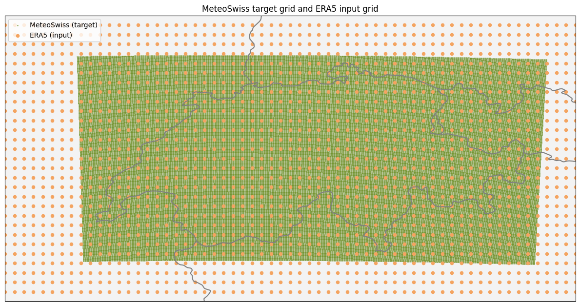
The preprocessing pipeline transforms the three raw datasets into the tensor representations consumed by the ConvCNP. Because the context input (ERA5-Land) and the target observations (MeteoSwiss) live on different grids, in different coordinate systems, and in different units, the main challenges are coordinate alignment, consistent normalization, and the construction of auxiliary features that help the model account for topographic effects. Figure 3.1 illustrates the spatial relationship between the two grids.
3.2.1 Data Quality and Cleaning
ERA5-Land is a reanalysis product: it is generated by assimilating historical observations into a numerical weather model under rigorous quality control by ECMWF. As a result, the data is spatially and temporally complete—there are no missing values, no gaps in the time series, and no outliers arising from instrument failures. Similarly, the MeteoSwiss TmaxD product is a quality-controlled gridded interpolation of station observations, and the swisstopo DHM25 is a professionally produced digital elevation model. Consequently, no ad-hoc cleaning, gap-filling, or outlier removal was required. The only data filtering applied was temporal subsetting: selecting either a single year (2023, 365 days) for rapid prototyping or a ten-year window (2014–2023, 3 650 days) for the primary experiments.
3.2.2 Coordinate Alignment and Regridding
The three datasets use two different coordinate reference systems. ERA5-Land uses a regular latitude–longitude grid in WGS84 (EPSG:4326), while both the MeteoSwiss observations and the swisstopo DEM use the Swiss LV95 projected coordinate system (EPSG:2056), whose axes are expressed in meters. Aligning these required two types of coordinate transformations, both performed using pyproj:
-
1.
MeteoSwiss ERA5 frame. The MeteoSwiss dataset provides latitude and longitude fields in WGS84 degrees alongside its native LV95 grid indices. These WGS84 coordinates are normalized to using the ERA5-Land bounding box, so that target locations are expressed in the same reference frame as the context grid.
-
2.
WGS84 LV95 for DEM lookup. To extract high-resolution elevation at each MeteoSwiss target point, the WGS84 target coordinates are transformed to LV95 meters, then used to query the swisstopo DEM and TPI fields via bilinear interpolation (xarray.DataArray.interp).
The ERA5-Land grid-cell elevation (derived from the geopotential field, see below) is similarly interpolated to target locations, but this interpolation uses the native WGS84 coordinates of the ERA5 grid since both the geopotential and the target latitude/longitude are in the same coordinate system.
3.2.3 Feature Engineering
Temperature Normalization
Both the ERA5-Land context temperatures and the MeteoSwiss target temperatures are normalized using a global Z-score computed from the ERA5-Land training data:
| (3.1) |
where and are the mean and standard deviation of the ERA5-Land t2m_max field over the entire training period. Using the same normalization for both context and target ensures that the model operates in a consistent scale. The MeteoSwiss data, originally in degrees Celsius, is first converted to Kelvin before applying the normalization.
Coordinate Normalization
Latitude and longitude are min–max normalized to using the ERA5-Land bounding box:
| (3.2) |
These normalized coordinates serve two roles: they form two of the five CNN input channels (enabling the model to learn position-dependent patterns), and they define the target locations passed to the decoder.
Cyclical Seasonal Encoding
The day of year is encoded as a pair of cyclical features:
| (3.3) |
This representation avoids the discontinuity that a raw day-of-year integer would introduce at the year boundary (day 365 day 1). These two channels are broadcast to the full spatial grid and appended to the ERA5-Land input tensor as channels 4 and 5. Additionally, the same seasonal features are optionally fed directly to the elevation MLP, allowing it to learn season-dependent lapse rate corrections (e.g. steeper gradients in summer versus temperature inversions in winter valleys).
Altitude from Geopotential
The ERA5-Land geopotential field (in m2 s-2) is converted to grid-cell altitude via:
| (3.4) |
This provides a coarse (11 km) estimate of the terrain height at each ERA5-Land grid cell. Since the geopotential is static, only the first time step is used. The resulting altitude field is interpolated to target locations via bilinear interpolation and used to compute the elevation difference feature described below.
High-Resolution Topographic Features
Three elevation-related features are computed at each MeteoSwiss target point and passed to the elevation MLP:
-
1.
True elevation (): bilinearly interpolated from the 25 m swisstopo DEM at the target’s LV95 coordinates.
-
2.
Elevation difference (): the difference between the true elevation and the ERA5-Land grid-cell elevation interpolated to the same point. This captures the local altitude mismatch that the coarse grid cannot resolve—for instance, a mountain peak that lies within a grid cell whose mean elevation is hundreds of meters lower.
-
3.
Topographic Position Index (TPI500): interpolated from the swisstopo TPI at a 500 m radius, quantifying whether a target point sits on a ridge (positive TPI), in a valley (negative TPI), or on an open slope (near-zero TPI). This encodes local terrain shape beyond what a single elevation value conveys.
These three features are stacked into a per-point elevation tensor of shape (n_points, 3), which the MLP uses to adjust the CNN’s base prediction for local topographic effects.
3.2.4 Context Tensor Assembly
The final ERA5-Land context tensor has shape (time, 5, 29, 61), where the five channels are:
-
1.
Normalized daily maximum temperature
-
2.
Normalized latitude
-
3.
Normalized longitude
-
4.
Cosine seasonal encoding
-
5.
Sine seasonal encoding
A pre-computed distance tensor of shape (n_target_points, 29, 61) stores the squared Euclidean distance from each target location to every ERA5-Land grid cell. This tensor is used by the set convolution encoder to weight context observations according to their proximity to each target.
3.2.5 Metadata Preservation for Reproducibility
All normalization statistics—the global mean and standard deviation of the ERA5-Land temperature field, the latitude and longitude bounding box, and the original coordinate arrays—are encapsulated in an Era5Metadata dataclass and serialized to JSON alongside each trained model. Similarly, the full training configuration (hyperparameters, ablation switches, data paths, and random seeds) is captured in a Params dataclass and persisted in the same manner. This ensures that any trained model can be loaded and used for inference with the exact normalization and configuration parameters that were used during training, without relying on the original data files being accessible. Both dataclasses support round-trip JSON serialization, including special handling for NumPy arrays in the metadata.
3.3 Model Selection and Implementation
3.3.1 Why a Convolutional Conditional Neural Process?
The downscaling task can be approached with methods ranging from bilinear interpolation to geostatistical kriging to fully convolutional super-resolution networks. The ConvCNP was selected for four reasons:
-
1.
Probabilistic output. The model predicts the parameters of a Gaussian distribution per target point, providing calibrated uncertainty estimates alongside point predictions.
-
2.
Translation equivariance. The convolutional architecture encodes the prior that spatial relationships are position-invariant—a sound inductive bias for meteorological fields.
-
3.
Flexible context conditioning. The set convolution encoder accepts variable numbers of context observations at arbitrary locations, making the model robust to missing data.
-
4.
End-to-end learning. All components are jointly trained by maximizing the log-likelihood of target observations, learning optimal internal representations directly from data.
3.3.2 Leveraging Vaughan et al. (2022)
This project builds on the open-source ConvCNP implementation of Vaughan et al. (2022) (Vaughan, 2022), which provided the encoder, ResNet decoder, MLP, training loop, loss functions, and evaluation metrics. Several elements had been adapted from Dubois’ Neural Process repository (Dubois, 2020).
Starting from this base, very few modifications were made to the code from Vaughan et al. (2022); a detailed list is included in the Appendix. Those python modules were used to build a separate set of libraries and tooling to adapt the model to the Swiss domain:
-
•
WGS84/LV95 coordinate handling;
-
•
using high-resolution topographic features;
-
•
using cyclical seasonal encodings.
3.3.3 Architecture Overview
The temperature downscaling model (TmaxBiasConvCNPElev, from Vaughan et al. (2022)) consists of four sequential stages:
-
1.
Encoder (set convolution). Maps the context tensor and a binary mask onto a representation per grid cell using convolutions (kernel size 5).
-
2.
CNN decoder (ResNet). Residual blocks with convolutions process the encoded grid, compressing the representation.
-
3.
Grid-to-point interpolation. An MLP maps the CNN output to at each grid cell. These are interpolated to the target points via an RBF kernel with learnable length scale , using a pre-computed distance tensor. The standard deviation is constrained to be strictly positive.
-
4.
Elevation MLP. The interpolated are concatenated with five auxiliary features—true elevation, elevation difference, TPI, and two seasonal encodings—and passed through an MLP that outputs topography- and season-corrected predictions.
3.3.4 Loss Function
The model is trained by maximizing the Gaussian log-likelihood:
| (3.5) |
where is the observed normalized temperature and are the predicted distribution parameters. NaN targets (points outside the Swiss border) are excluded. If we look at the following expansion:
| (3.6) |
we realize that this objective incentivizes both accurate means and well-calibrated uncertainty: overconfident predictions are penalized by the term, while underconfident predictions are penalized by the squared-error term.
3.3.5 Experimental Setup
Temporal -Fold Cross-Validation
The dataset is split temporally: a 5-fold scheme divides the time series into contiguous blocks, holding out one block for validation per fold (73 days each for the single-year dataset). For each fold, training days are shuffled and batched, the held-out fold is evaluated after every epoch (NLL, MAE, Pearson and Spearman correlations), the best checkpoint is saved by validation NLL, and early stopping halts training after 10 epochs without improvement.
Hyperparameters
| Category | Parameter | Value |
| Architecture | CNN channels† | 128 |
| ResConvBlocks† | 6 | |
| Kernel size† | 5 | |
| RBF length scale† | 0.1 | |
| MLP | Hidden layers† | 4 |
| Units per layer† | 64 | |
| Training | Learning rate† | |
| Optimizer | Adam | |
| Batch size | 16 (local) / 8 (Renku) | |
| Max epochs | 10 / 30 (default) / 100 | |
| Early stopping patience | 10 | |
| Validation | Folds | 5 |
| Split strategy | Temporal (contiguous) | |
| Reproducibility | Seed | 42 |
Individual models may have been trained with different hyperparameters.
For each model, all hyperparameters were stored in a file named
trained_models/<model_name>/metadata.json.
3.3.6 Ablation Experiments
To isolate the contribution of individual components, ablation experiments toggle feature flags in the configuration while keeping all other hyperparameters and cross-validation splits identical:
-
•
No MTPI (USE_MTPI=False): MTPI is excluded from the elevation MLP.
-
•
No elevation (USE_ELEVATION=False): the elevation MLP receives only the CNN’s base prediction, isolating the CNN’s downscaling skill fully from all topographic correction.
-
•
No seasonal in MLP (SEASONAL_FEATURES_IN_MLP=False): seasonal features remain in the CNN input but are withheld from the elevation MLP.
-
•
No seasonal (SEASONAL_FEATURES=False): cyclical day-of-year channels are removed entirely, forcing the model to make its predictions without knowing which time in the year it is. Weather behaviour at altitude varies greatly depending on the seasons.
3.4 Models Trained and Metrics Captured
All trained models reside under trained_models/, with each directory name encoding the key experimental variables following the convention:
final-YYYY-Ne-Kf [-ablation-component]
where YYYY is the first year of training data (all datasets end in 2023), N is the maximum number of training epochs, K is the number of cross-validation folds, and the optional -ablation-component suffix identifies the disabled feature. For example, final-2014-30e-5f denotes a model trained on 2014–2023 data for up to 30 epochs with 5-fold temporal cross-validation and all features enabled.
Nine model configurations were trained in total, organized into two groups: primary models that vary data volume and training duration with all features enabled, and ablation models that each disable one component to isolate its contribution. All models share the architecture and hyperparameters listed in Table 3.2 (Section 3.3.5), differing only in the parameters described below.
3.4.1 Primary Models
The primary experiments study two axes: the effect of training duration (10, 30, and 100 epochs on a single year of data) and the effect of data volume (1 year versus 10 years at a fixed epoch budget). Table 3.3 summarizes the four completed configurations.
| Model name | Data range | Days | Epochs | Batch size |
| final-2023-10e-5f | 2023 only | 365 | 10 | 8 |
| final-2023-30e-5f | 2023 only | 365 | 30 | 8 |
| final-2023-100e-5f | 2023 only | 365 | 100 | 8 |
| final-2014-30e-5f | 2014–2023 | 3 652 | 30 | 8 |
A fifth configuration, final-2004-30e-5f, attempted to extend the training window to twenty years (2004–2023). The larger dataset required reducing the batch size from 8 to 4 to fit within GPU memory. Only one of five cross-validation folds completed before the computational budget was exhausted; this model was not carried forward to evaluation and is excluded from subsequent results.
3.4.2 Ablation Models
To isolate the contribution of individual model components, four ablation experiments were conducted on the ten-year dataset (2014–2023, 30 epochs, 5 folds). Each ablation disables exactly one feature relative to the fully-featured baseline (final-2014-30e-5f). Table 3.4 lists the configurations and indicates which features are enabled (✓) or disabled (–) in each variant.
| Ablation suffix | Elev. | TPI | Season. (CNN) | Season. (MLP) |
| (none—baseline) | ✓ | ✓ | ✓ | ✓ |
| -ablation-elevation | – | – | ✓ | ✓ |
| -ablation-mtpi | ✓ | – | ✓ | ✓ |
| -ablation-seasonal-all | ✓ | ✓ | – | – |
| -ablation-seasonal-in-mlp | ✓ | ✓ | ✓ | – |
Disabling elevation (USE_ELEVATION=False) also disables TPI, since TPI is an input to the elevation MLP (Section 3.3.3). This variant therefore removes the entire topographic correction stage, and the model’s output relies solely on the CNN decoder’s grid-to-point interpolation.
3.4.3 Metrics Captured
Each evaluation run—covering all five cross-validation folds—produces a JSON file following the naming convention metrics-INPUT-SPARSITY-value.json (see Appendix for the full specification). The recorded metrics fall into four groups:
- Point accuracy.
-
Mean Absolute Error (MAE), Root Mean Squared Error (RMSE), and mean bias, all in °C.
- Probabilistic skill.
-
The Continuous Ranked Probability Score (CRPS) and a skill score relative to deterministic ERA5-Land bilinear interpolation:
(3.7) where the reference CRPS equals the MAE of the bilinear baseline (since the CRPS of a deterministic forecast reduces to its mean absolute error). A skill score of 0 indicates parity with the baseline; positive values indicate improvement.
- Correlations.
-
Pearson correlations between predicted uncertainty () and absolute error, between altitude and error, between mTPI and error, and between day-of-year and error.
- Calibration.
-
Probability Integral Transform (PIT) mean and standard deviation, observed coverage at the 50%, 90%, and 95% nominal levels, the Kolmogorov–Smirnov -value, and the Mean Absolute Calibration Error (MACE), to track the reliability of the uncertainty estimates.
3.4.4 Predictions on sparse gridded input
For gridded input, a sparse grid of ERA5-Land was offered the model as input to predict the full target grid. Different sparsity levels were captured.
3.4.5 Predictions on sparse out-of-grid input
For out-of-grid input (sampled from the MeteoSwiss target dataset), the points are regridded onto the training grid (ERA5-Land) and then fed to the model for full target grid prediction. Given the rugged Swiss topography, this approach is expected to cause a massive reduction in model performance.
Please see section A.6 in the Appendix for considerations on how to better handle out-of-grid inputs.
3.4.6 Technology Stack
The project is implemented in Python on the following stack:
-
•
PyTorch for model definition, training, and GPU inference.
-
•
xarray and Dask for lazy-loading and processing of NetCDF/Zarr datasets.
-
•
pyproj for WGS84 / LV95 coordinate transformations.
-
•
scipy and scikit-learn for evaluation metrics and preprocessing.
-
•
Renku (Swiss Data Science Center, ) (SDSC) for reproducible environments, GPU cloud sessions (NVIDIA MIG partitions), and version control.
Reproducibility is enforced by seeding all random number generators (Python, NumPy, PyTorch, CUDA) with a fixed seed and setting cudnn.deterministic=True.
Chapter 4 Results and Evaluation
4.1 Experimental Results
This section demonstrates that the ConvCNP training procedure converges reliably and that the resulting model produces physically plausible downscaled predictions. Detailed quantitative evaluation follows in subsequent sections.
4.1.1 Training Convergence

Figure 4.1 shows the training curves for the primary ten-year model
(final-2014-30e-5f), averaged across all five cross-validation folds. The left panel tracks Pearson and Spearman correlation on a logarithmic residual scale (); the right panel shows the validation MAE (in normalized units) alongside the training and validation negative log-likelihood (NLL).
Three convergence trends are evident:
-
1.
Error reduction. The validation MAE drops steeply during the first five epochs—from to in normalized units—and continues to decrease more gradually thereafter, reaching by epoch 30. All five folds exhibit the same pattern with tight variance: the best per-fold MAE values cluster around , indicating consistent convergence.
-
2.
Correlation improvement. Both Pearson and Spearman correlations start high—above 0.967 already at epoch 0, reflecting the strong spatial structure in the temperature field—and improve to by the end of training.
-
3.
Loss decrease. The training and validation NLL both decrease from positive values () to negative values (), indicating that the model learns to assign increasingly high likelihood to the observed targets. The two curves track each other closely throughout, with no divergence between them—a sign that overfitting is not occurring. No fold triggered early stopping; all five ran for the full 30 epochs, and the best checkpoints were selected between epochs 18 and 29, suggesting that marginal gains were still accumulating toward the end of training. This is further confirmed by the experiment running for up to 100 epochs (see below).
4.1.2 Sample Prediction

Figure 4.2 illustrates a single-day prediction from the fifth cross-validation fold.
The input panel shows the smooth, coarse-resolution temperature field from ERA5-Land, in which topographic detail is largely absent. The ground-truth panel reveals the fine-grained spatial structure that the model must recover: sharp temperature gradients along the Alpine ridge, cold mountain peaks, and warmer valleys—features well below the resolution of the input grid.
The prediction panel demonstrates that the model successfully reconstructs much of this detail. The overall spatial pattern closely follows the ground truth, with the major valleys, plateaus, and high-altitude regions clearly resolved. The bias panel confirms that residual errors are small across most of the domain (near-white shading), with the largest deviations concentrated in high-mountain areas where the elevation gradient is steepest.
4.2 Performance
4.2.1 Global metrics
Here are visualizations of the errors, error bias, CRPS and skill for the baseline model (10 years of data, 30 epochs, 5 folds, no ablation, aggregate results over the folds).

 |
 |
| Model | MAE | RMSE | Bias | CRPS | Skill |
| (°C) | (°C) | (°C) | (°C) | ||
| Primary models | |||||
| 2023-10e-5f | 2.09 | 2.67 | 0.66 | 1.90 | 0.245 |
| 2023-30e-5f | 1.64 | 2.08 | 0.24 | 1.49 | 0.410 |
| 2023-100e-5f | 1.62 | 2.05 | 0.25 | 1.48 | 0.415 |
| 2014-30e-5f (base model) | 1.31 | 1.71 | 0.05 | 1.21 | 0.524 |
Table 4.1 summarises the headline accuracy and skill metrics for all evaluated models on the full ERA5-Land grid (1 769 context points). Each row reports the mean absolute error (MAE), root-mean-square error (RMSE), and mean bias of the point prediction in degrees Celsius, together with the Continuous Ranked Probability Score (CRPS) and a skill score defined as , where the reference is the deterministic bilinear interpolation of ERA5-Land to the target grid (for a deterministic forecast, ). A skill of 0 indicates no improvement over the interpolation baseline; a skill of 1 would indicate a perfect forecast.
Effect of training duration.
The three single-year models (trained on 2023 data, evaluated on 365 holdout days) isolate the effect of longer optimisation. Increasing from 10 to 30 epochs cuts the MAE from 2.09 to 1.64 °C (a 22% reduction) and nearly doubles the skill score from 0.245 to 0.410. Extending training further to 100 epochs yields only a marginal additional gain (MAE 1.62 °C, Skill 0.415), suggesting that most of the representational capacity available to the single-year model is utilised within the first 30 epochs. Even though the slowdown was found, up to 100 epochs convergence continues without signs of overfitting.
Effect of training data volume.
Moving from one year to ten years of training data (both at 30 epochs) produces the largest single improvement: the MAE drops from 1.64 to 1.31 °C, the RMSE from 2.08 to 1.71 °C, and the skill score rises from 0.410 to 0.524. The mean bias also shrinks to near zero (0.05 °C). These gains indicate that additional climatological diversity—exposing the model to a wider range of synoptic situations and seasonal extremes—is more beneficial than additional gradient steps on a limited sample.
Skill relative to ERA5-Land interpolation.
All primary models improve upon the bilinear-interpolation baseline. The ten-year model achieves a CRPS-based skill of 0.524, meaning its probabilistic predictions reduce the expected error by more than half compared to simply interpolating the coarse reanalysis field. Even the weakest model (10 epochs, single year) attains a skill of 0.245, confirming that the ConvCNP learns meaningful fine-scale structure beyond what spatial interpolation alone can provide.
Uncertainty calibration.
 |
 |
 |
 |
Figure 4.5 shows Q–Q plots of the Probability Integral Transform (PIT) for each primary model. A perfectly calibrated model would produce PIT values uniformly distributed on , yielding points along the diagonal. All four models exhibit a pronounced S-shaped departure: the empirical quantiles rise steeply, the standardised residual standard deviation (-std) is approximately 8.7 (ideal: 1.0), confirming that the model is overconfident by roughly an order of magnitude.
This miscalibration is consistent across all configurations and may arise from the Gaussian likelihood training objective, which optimises overall fit rather than interval coverage.
4.2.2 Correlations

Despite the overconfidence mentioned above, the model’s predicted uncertainties remain informative: the correlation between predicted and absolute error is 0.74 for the ten-year model, meaning that the uncertainty estimates reliably rank predictions by quality even though their absolute magnitudes are too small.

It is known that weather prediction at altitude is a tough problem. The correlation between altitude and error exists, but is significantly lower than the one observed between predicted uncertainty and error.

We can observe the colder months (November–March) observe a higher incidence of outliers in mean absolute error.
4.3 Ablation Analysis
| Model | MAE | RMSE | Bias | CRPS | Skill |
| (°C) | (°C) | (°C) | (°C) | ||
| Primary model (2014–2023) | |||||
| 2014-30e-5f (base model) | 1.31 | 1.71 | 0.05 | 1.21 | 0.524 |
| Ablation models (2014–2023) | |||||
| -ablation-elevation | — model diverged; see text — | ||||
| -ablation-mtpi | 1.33 | 1.74 | 0.13 | 1.23 | 0.517 |
| -ablation-seasonal-all | 1.38 | 1.80 | 0.12 | 1.27 | 0.50 |
| -ablation-seasonal-in-mlp | 1.29 | 1.69 | 0.08 | 1.19 | 0.532 |
Without the elevation MLP, the model produced errors orders of magnitude above physical plausibility (MAE 802 °C), indicating that the topographic correction stage is essential for meaningful predictions. (This is unexpected, we would expect some degree of interpolation to still take place.)
All ablation models use the same ten-year dataset (2014–2023), 30 training epochs, five-fold cross-validation, and identical splits as the base model. Each experiment disables a single feature group while keeping everything else unchanged, so that differences in the metrics can be attributed to that component alone.
Elevation features.
Removing the three topographic inputs—true elevation, elevation difference, and TPI—from the elevation MLP (USE_ELEVATION=False) caused the model to diverge catastrophically. The resulting MAE of °C and a negative skill score of indicate that the predictions are off-scale by orders of magnitude. Notably, the altitude–error correlation jumps from 0.19 in the base model to 0.78 in this ablation, confirming that the errors are overwhelmingly concentrated at locations where the true elevation differs most from the coarse ERA5-Land grid-cell elevation. Without topographic correction, the elevation MLP receives only the CNN’s interpolated and zero-valued placeholders; it has no mechanism to compensate for the fact that a 3 000 m peak and a 400 m valley within the same 11 km grid cell receive nearly identical CNN predictions. The MLP, trained on these uninformative inputs, learns weight configurations that produce numerically unstable outputs at evaluation time—when all 46 000+ target points are predicted simultaneously—resulting in the observed divergence. This outcome confirms that the elevation MLP is not merely a refinement stage but the essential component that bridges the resolution gap between the coarse reanalysis grid and the fine-scale target field. The author must also consider that there may have been some misconfiguration or bug which could cause this, but one was not identified.
Topographic Position Index.
Removing only the TPI channel
(USE_MTPI=False) while retaining true elevation and elevation difference has a marginal effect: the MAE increases from 1.31 to 1.33 °C and the skill score decreases from 0.524 to 0.517. The bias shifts from to °C, a small systematic cold bias. This suggests that TPI—which encodes whether a target lies on a ridge, in a valley, or on an open slope—provides a secondary, but not essential, correction on top of the elevation difference. The elevation difference alone captures most of the sub-grid topographic variance.
Seasonal features.
Two ablations target the cyclical day-of-year encoding (/ channels). The first (-ablation-seasonal-all) removes them everywhere: both from the CNN input channels and from the elevation MLP. We can see fully ablating time-of-year encoding (both in the spatially-aware CNN and the MLP) has a significant impact on model performance.
Seasonal feature ablation from the MLP outperforms the base model.
Counter-intuitively, this ablation achieve slightly better metrics than the base model (MAE 1.29 vs. 1.31 °C; Skill 0.532 vs. 0.524). The improvement is small but consistent across all metrics. This likely reflects a mild regularisation effect: the base model’s elevation MLP has 7 inputs (including /), while the seasonal ablations have only 5, reducing the MLP’s capacity to overfit to spurious correlations between the seasonal encoding and the residual error. Alternatively, feeding redundant features to the MLP may slightly impede optimisation by diluting the gradient signal from the more informative elevation inputs. In either case, the practical difference is modest, and the result suggests that removing the explicit seasonal features is, if anything, slightly beneficial. This also suggests the MLP might be constrained and might capture more differentiable signal from the training data if we increase its size.
4.4 Performance on sparse input, on- and off-grid
A key question for real-world deployment is how the model behaves when the full ERA5-Land grid is unavailable and only a sparse set of observations is provided as context. We evaluate two scenarios: (i) on-grid sparsity, where a random subset of ERA5-Land grid cells is retained, and (ii) off-grid sparsity, where the context consists of MeteoSwiss ground-station observations placed onto the nearest ERA5 grid cell. In both cases the model weights are frozen—no retraining is performed—so the results measure zero-shot robustness to reduced input.
4.4.1 On-grid sparsity (ERA5-Land)
| Input | Points | MAE | RMSE | Bias | CRPS | Skill | –err |
| (°C) | (°C) | (°C) | (°C) | corr | |||
| 20 pts | 20 | 4.93 | 6.09 | 1.81 | 4.83 | 0.903 | 0.111 |
| 50 pts | 50 | 3.73 | 4.66 | 1.73 | 3.63 | 0.430 | 0.012 |
| 80 pts | 80 | 3.20 | 4.02 | 1.69 | 3.10 | 0.223 | 0.023 |
| 100 pts | 100 | 2.99 | 3.75 | 1.59 | 2.89 | 0.140 | 0.026 |
| 120 pts | 120 | 2.77 | 3.48 | 1.43 | 2.67 | 0.052 | 0.010 |
| 10% (177) | 177 | 2.27 | 2.86 | 1.01 | 2.17 | 0.144 | 0.002 |
| 25% (442) | 442 | 1.51 | 1.93 | 0.20 | 1.41 | 0.446 | 0.272 |
| 50% (885) | 885 | 1.36 | 1.77 | 0.01 | 1.26 | 0.505 | 0.668 |
| 90% (1 592) | 1 592 | 1.31 | 1.72 | 0.04 | 1.21 | 0.522 | 0.736 |
| 100% (1 769) | 1 769 | 1.31 | 1.71 | 0.05 | 1.21 | 0.524 | 0.740 |
Table 4.3 summarises the model’s performance as the fraction of retained ERA5-Land grid cells decreases from 100% to as few as 20 points.
Graceful degradation at moderate sparsity.
Halving the input grid to 50% (885 points) increases the MAE by only 3.8%, from 1.31 to 1.36 °C, and the skill score drops marginally from 0.524 to 0.505. At 25% of the grid (442 points), the MAE rises to 1.51 °C (+15%) but the skill remains strongly positive at 0.446, meaning the model still substantially outperforms bilinear interpolation. These results demonstrate that the ConvCNP’s convolutional encoder can extract useful spatial structure even from heavily subsampled gridded input.
Transition to negative skill.
At 10% of the grid (177 points), the MAE increases to 2.27 °C (+74%) and the skill drops to 0.144—still positive, but the model’s advantage over the interpolation baseline is diminishing rapidly. Below 177 points, the skill turns negative: at 120 points it is 0.052 and at 20 points it reaches 0.903, indicating that the model performs worse than simple bilinear interpolation. The crossover occurs between approximately 120 and 177 ERA5 grid points.
Uncertainty estimates collapse.
At the full grid, the correlation between predicted and absolute error is 0.74, indicating highly informative uncertainty estimates. This correlation degrades smoothly—0.67 at 50%, 0.27 at 25%—and effectively vanishes below 10% (0.002 at 177 points). For the absolute-count configurations (20–120 points), the –error correlation hovers near zero, meaning the model’s uncertainty estimates are no longer informative. This is consistent with the CNN receiving too little spatial context to distinguish uncertain from confident predictions.
Systematic warm bias.
At full coverage the model exhibits near-zero bias (0.05 °C). As context is removed, a systematic warm bias emerges: 0.20 °C at 25%, 1.01 °C at 10%, and 1.81 °C at 20 points. When the CNN receives too few observations to reconstruct the spatial temperature pattern, the elevation MLP’s residual correction—trained to compensate for the difference between the coarse ERA5 grid-cell temperature and the fine-scale target—reverts toward a warm-biased default.

Figure 4.9 shows the degradation curves for both input types. The ERA5 on-grid curve exhibits a clear elbow around 25–50% of the grid: above this range the model is near-optimal; below it, performance degrades rapidly.
4.4.2 Off-grid sparsity (MeteoSwiss target set)
| Input | Points | MAE | RMSE | Bias | CRPS | Skill | –err |
| (°C) | (°C) | (°C) | (°C) | corr | |||
| 20 pts | 20 | 4.77 | 5.78 | 2.05 | 4.67 | 0.840 | 0.047 |
| 50 pts | 50 | 3.54 | 4.24 | 2.26 | 3.44 | 0.356 | 0.178 |
| 80 pts | 80 | 2.99 | 3.56 | 1.98 | 2.89 | 0.137 | 0.135 |
| 100 pts | 100 | 2.84 | 3.38 | 1.86 | 2.74 | 0.079 | 0.125 |
| 120 pts | 120 | 2.79 | 3.31 | 1.92 | 2.69 | 0.060 | 0.128 |
| 176 pts | 176 | 2.68 | 3.16 | 2.07 | 2.58 | 0.018 | 0.124 |
Table 4.4 presents results when the ERA5-Land grid is replaced entirely by MeteoSwiss metrics mapped onto the nearest ERA5 grid cell. This tests whether the model can operate from sparse, irregularly placed, off-grid measurements—a scenario closer to real-world station-based downscaling.
Negative skill at all densities.
Even with all 176 available MeteoSwiss stations, the model achieves a skill of only 0.018—marginally worse than bilinear interpolation of the ERA5 field. At 20 stations the skill drops to 0.840. The model never outperforms the interpolation baseline in this configuration. Though this comparison is somewhat unfair: there is no real-time feed of a complete ERA5-Land grid; it only becomes available later after systemic and painstaking reanalysis.
Persistent warm bias.
All MeteoSwiss configurations exhibit a large, stable warm bias between 1.86 and 2.26 °C. Unlike the ERA5 on-grid case where the bias grows with sparsity, here the bias is approximately constant across all point counts. This suggests a systematic offset: MeteoSwiss stations, which are predominantly located in valleys and at lower elevations, provide a biased sample of the temperature field. The model, trained on full ERA5 grids, has no mechanism to correct for this sampling bias at inference time.
Uninformative uncertainty.
The –error correlation is negative across all MeteoSwiss configurations (0.05 to 0.18), meaning the model’s predicted uncertainty is slightly anti-correlated with the actual error. The model’s uncertainty machinery, trained on dense gridded input, produces meaningless confidence estimates when the input distribution shifts to sparse off-grid points.
4.4.3 On-grid vs. off-grid at comparable point counts

At matched point counts (20, 50, 80, 100, 120), the ERA5 on-grid and MeteoSwiss off-grid configurations yield surprisingly similar MAE values—within 0.02–0.22 °C of each other. At very low counts (20–80 points), MeteoSwiss actually achieves slightly lower MAE than ERA5 on-grid (e.g. 4.77 vs. 4.93 °C at 20 points), likely a bias introduced because MeteoSwiss points are actually used as ground truth. However, this MAE advantage does not translate to positive skill, because the MeteoSwiss configurations suffer from a much larger systematic bias (2 °C vs. 1.4–1.8 °C for ERA5 at the same counts).

Figure 4.11 confirms that the model’s overconfidence, already identified at full coverage (-std 8.7), worsens dramatically as input density decreases: -std reaches 35 at 20 ERA5 points and 34 at 20 MeteoSwiss stations. The 90% prediction interval coverage, already far below the nominal 90% at full coverage (16.5%), drops to 4.3% at 20 ERA5 points. This reinforces that the Gaussian likelihood training objective does not produce well-calibrated uncertainties, and the miscalibration is amplified when the model operates outside its training distribution.
Representative single-day prediction maps for all sparsity configurations—showing the progressive visual degradation of the input field, the model prediction, and the residual bias—are collected in Appendix A.7.
4.5 Discussion of Results
This section revisits the four research questions posed in the introduction in light of the experimental evidence presented above.
Model viability.
The ConvCNP, adapted from the UK-focused implementation of Vaughan et al. (2022) and equipped with high-resolution Swiss topographic features, produces accurate downscaled temperature fields over Switzerland. The best model achieves an MAE of 1.31 °C and an RMSE of 1.71 °C across roughly 3 650 holdout days, with near-zero mean bias (0.05 °C). The spatial structure of the predictions closely matches the MeteoSwiss ground truth, resolving Alpine valleys, ridges, and plateaus that are invisible at the ERA5-Land resolution. These results confirm that the architecture transfers successfully to the topographically complex Swiss domain.
Skill over interpolation.
All primary models outperform bilinear interpolation of the ERA5-Land grid. Even the weakest configuration (single year, 10 epochs) achieves a CRPS-based skill of 0.245, while the ten-year model reaches 0.524—reducing the expected probabilistic error by more than half relative to the interpolation baseline. This demonstrates that the ConvCNP learns meaningful fine-scale structure that pure spatial interpolation cannot capture.
Feature importance.
The ablation study reveals a clear hierarchy of feature contributions. The elevation MLP and its topographic inputs are indispensable: removing them causes the model to diverge catastrophically (MAE 802 °C), confirming that the MLP is not a refinement but the essential component bridging the coarse-to-fine resolution gap. The Topographic Position Index provides a small but measurable benefit (MAE increases by 0.02 °C without it), consistent with its role as a secondary terrain descriptor. The seasonal features present a more nuanced picture: removing them from the MLP slightly improves performance (MAE 1.29 vs. 1.31 °C), suggesting a mild regularisation benefit from reducing the MLP’s input dimensionality. Furthermore, the two seasonal ablations—removing seasonal features everywhere versus only from the MLP—produce bit-identical results, indicating that the CNN entirely ignores the explicit seasonal channels in its input. The temperature field itself evidently carries sufficient seasonal signal for the CNN, while the MLP benefits from a leaner feature set.
Scaling behaviour.
Two scaling axes were investigated: training duration and data volume. Increasing epochs from 10 to 30 yields a 22% MAE reduction (2.09 to 1.64 °C), but extending to 100 epochs provides only marginal further gains (1.62 °C), indicating that the single-year model saturates its representational capacity within roughly 30 epochs. Importantly, no overfitting is observed even at 100 epochs. In contrast, moving from one year to ten years of training data at the same epoch count produces the largest single improvement (MAE from 1.64 to 1.31 °C; Skill from 0.410 to 0.524), demonstrating that climatological diversity—exposure to varied synoptic situations and seasonal extremes—is more valuable than additional gradient steps on limited data. This suggests that further performance gains may be achievable by training on the full ERA5-Land archive (1950–present).
Robustness to sparse input.
The model degrades gracefully when the ERA5-Land input grid is subsampled: at 50% density the MAE increases by only 3.8%, and positive skill is maintained down to approximately 10% of the grid (177 points). Below this threshold, skill turns negative and the model performs worse than bilinear interpolation. Replacing the ERA5 grid entirely with MeteoSwiss station observations (off-grid, snapped to the nearest grid cell) yields negative skill at all tested densities, accompanied by a persistent warm bias of 2 °C. This reflects both the distribution shift (the model was trained on dense gridded input) and the valley-biased sampling of the Swiss station network. The uncertainty estimates, which are highly informative at full coverage (–error correlation of 0.74), collapse to near-zero correlation below 10% density and become anti-correlated for off-grid input.
Uncertainty calibration.
Despite the model’s strong point-prediction performance, its uncertainty estimates are severely overconfident across all configurations: the predicted underestimates the true error magnitude by roughly an order of magnitude (-std 8.7 at full coverage). The 90% prediction interval covers only 16.5% of observations. This miscalibration, consistent across training configurations and worsening with sparser input, is a known limitation of the Gaussian likelihood objective, which optimises overall fit rather than interval coverage. Nonetheless, the ranking of uncertainties remains informative: the model reliably assigns higher to locations where it makes larger errors, even though the absolute magnitudes are too small.
Chapter 5 Conclusion and Future Work
5.1 Conclusion
This project set out to assess whether Convolutional Conditional Neural Processes—originally demonstrated for UK climate downscaling by Vaughan et al. (2022)—can produce accurate, uncertainty-aware temperature predictions over the topographically complex terrain of Switzerland. The answer is affirmative: the ConvCNP, equipped with a high-resolution elevation MLP, achieves an MAE of 1.31 °C and a CRPS-based skill of 0.524, reducing the expected prediction error by more than half compared to bilinear interpolation of the ERA5-Land grid. The model resolves fine-scale spatial structure—Alpine valleys, ridges, and plateaus—that is invisible at the 11 km input resolution.
Scaling experiments reveal that training data volume is the dominant lever for improvement: moving from one to ten years of data yields a larger gain than tripling the number of training epochs, and no overfitting is observed even at 100 epochs. The ablation study confirms that the elevation MLP is the essential architectural component—without it, the model diverges entirely—while TPI provides a small secondary benefit and explicit seasonal features in the MLP are slightly detrimental, suggesting a regularisation advantage from a leaner feature set.
The model degrades gracefully under sparse on-grid input, maintaining positive skill down to approximately 10% of the ERA5-Land grid. However, zero-shot deployment on off-grid MeteoSwiss station observations does not achieve positive skill at any tested density, highlighting the distribution shift between the dense gridded training regime and sparse irregular inference. Uncertainty calibration remains an open challenge: all configurations are severely overconfident, though the ranking of predicted uncertainties is informative.
5.2 Limitations
-
1.
Data breadth. Compared to Vaughan et al. (2022), this project uses fewer input channels: only temperature, coordinates, and seasonal encodings for the CNN, plus topographic features for the MLP. The original study additionally included geopotential height, wind fields, and humidity as CNN input channels. The narrower feature set likely limits the model’s ability to capture atmosphere-driven local effects such as Föhn winds.
-
2.
Uncertainty calibration. The model’s predicted uncertainties are overconfident by roughly an order of magnitude (-std 8.7; 90% interval coverage of only 16.5%). This is a known limitation (Guo et al. (2017)) of the Gaussian log-likelihood training objective, which concentrates gradient signal around the mean rather than penalising miscalibrated quantiles uniformly. Increasing training data volume from one to ten years did not resolve this issue, suggesting it is structural rather than data-limited.
-
3.
Evaluation against a gridded product. The MeteoSwiss ground truth is itself an interpolated product, not raw station measurements, and it does not align to the training grid. Errors in the ground-truth interpolation propagate into the evaluation metrics. And the bias of using a portion of the ground-truth to predict all the ground truth also seeps in.
-
4.
Elevation-agnostic CNN. As mentioned in the background section, in this project all topographic information is supplied exclusively through the elevation MLP, not the CNN itself. elevation-agnostic. This architectural difference may partly explain why the elevation MLP is so critical in our configuration: it bears the full burden of topographic correction, with no elevation-aware spatial context from the CNN to build upon.
-
5.
Single variable. Only daily maximum temperature was downscaled. For scoping reasons, minimum and average were not explored. The architecture supports precipitation via a Bernoulli–Gamma output layer, but this path was not exercised and may require additional work to wire correctly.
5.3 Future Work
The findings and limitations of this project suggest several directions for further development.
Geopotential as a CNN channel.
The most immediate architectural change would be to include the ERA5-Land geopotential field directly as a CNN input channel, following Vaughan et al. (2022). This would give the convolutional encoder access to coarse elevation context during spatial processing, potentially reducing the burden on the elevation MLP and improving predictions in areas where the coarse grid poorly represents the terrain.
Improved uncertainty calibration.
Replacing the Gaussian log-likelihood with a CRPS-based loss function could address the overconfidence at its root: CRPS penalises miscalibrated quantiles more evenly across the distribution, tending to produce wider, better-calibrated prediction intervals.
Additional input channels.
The model currently lacks atmospheric context beyond temperature. Integrating wind fields, humidity, and surface pressure as CNN channels—as well as terrain-derived features such as aspect and land cover—would provide the model with physically relevant information about local meteorological processes. These additions follow the extension points documented in Appendix A.5.
Multi-scale topographic features.
Currently only TPI at 500 m radius is used. Including TPI at additional scales (e.g. 2 000 m, also provided in swisstopo DHM25) would encode both local and wider topographic context, allowing the model to distinguish situations such as a hill within a deep valley from a hill on open plains—a distinction relevant for phenomena like cold-air pooling and valley inversions.
Larger elevation MLP.
The observation that removing seasonal features from the MLP slightly improves performance suggests the MLP may be capacity-constrained. Increasing its width or depth could allow it to capture more complex nonlinear interactions between elevation, terrain shape, and atmospheric conditions, and might also improve uncertainty calibration by giving the network more expressive power for the output.
Temporal context windows.
The current model processes each day independently. Providing a temporal window of consecutive grids as input would allow the CNN to track the movement and evolution of weather systems—e.g. the progression of cold fronts across the Alps—potentially improving predictions during rapidly changing conditions.
Climate-aware temporal encoding.
Including a year embedding alongside the seasonal encoding would allow the model, when trained over multi-decadal archives, to account for long-term climate trends such as rising temperatures and glacier retreat—effects that are relevant over the full ERA5-Land record (1960–present) but invisible to a purely seasonal encoding.
Hourly resolution and diurnal cycles.
Switching from daily to hourly datasets and including time-of-day embeddings would be necessary if this technology is to support real-time prediction from live station feeds—a direction of potential interest to SDSC and operational meteorological services.
Precipitation downscaling.
The ConvCNP architecture supports precipitation via a Bernoulli–Gamma output layer, as demonstrated by Vaughan et al. (2022). Extending the pipeline to precipitation downscaling is a natural next step, though it introduces additional complexity from the mixed discrete-continuous nature of rainfall.
Native off-grid support.
Deploying the model operationally on sparse station data requires moving beyond the current snap-to-grid approach. Architectural options—including a true set convolution encoder, attention-based mechanisms, and dual-stream architectures—are discussed in detail in Appendix A.6.
Training infrastructure.
Renku GPU sessions are occasionally interrupted during multi-day training runs for inscrutable reasons. Implementing checkpoint-based fold resumption—allowing training to restart from the middle of a fold rather than from the beginning—would improve robustness and reduce wasted compute.
References
- Vaughan et al. (2022) Anna Vaughan, Will Tebbutt, J. Scott Hosking, and Richard E. Turner. Convolutional conditional neural processes for local climate downscaling. Geoscientific Model Development, 15:251–268, 2022. doi: 10.5194/gmd-15-251-2022.
- Garnelo et al. (2018a) Marta Garnelo, Jonathan Schwarz, Dan Rosenbaum, Fabio Viola, Danilo J. Rezende, S. M. Ali Eslami, and Yee Whye Teh. Neural processes. arXiv preprint arXiv:1807.01622, 2018a. URL https://arxiv.org/abs/1807.01622.
- Gordon et al. (2020) Jonathan Gordon, Wessel P. Bruinsma, Andrew Y. K. Foong, James Requeima, Yann Dubois, and Richard E. Turner. Convolutional conditional neural processes. arXiv preprint arXiv:1910.13556, 2020. URL https://arxiv.org/abs/1910.13556.
- Garnelo et al. (2018b) Marta Garnelo, Dan Rosenbaum, Christopher Maddison, Tiago Ramalho, David Saxton, Murray Shanahan, Yee Whye Teh, Danilo J. Rezende, and S. M. Ali Eslami. Conditional neural processes. arXiv preprint arXiv:1807.01613, 2018b. URL https://arxiv.org/abs/1807.01613.
- Kim et al. (2019) Hyunjik Kim, Andriy Mnih, Jonathan Schwarz, Marta Garnelo, Ali Eslami, Dan Rosenbaum, Oriol Vinyals, and Yee Whye Teh. Attentive neural processes. arXiv preprint arXiv:1901.05761, 2019. URL https://arxiv.org/abs/1901.05761.
- Muñoz Sabater (2019) Joaquín Muñoz Sabater. ERA5-Land hourly data from 1950 to present. Copernicus Climate Change Service (C3S) Climate Data Store (CDS), 2019. URL https://cds.climate.copernicus.eu/datasets/reanalysis-era5-land.
- (7) MeteoSwiss. Daily mean, minimum and maximum temperature: TabsD, TminD, TmaxD. MeteoSwiss Grid-Data Products, Federal Office of Meteorology and Climatology, Switzerland. URL https://www.meteoswiss.admin.ch/dam/jcr:818a4d17-cb0c-4e8b-92c6-1a1bdf5348b7/ProdDoc_TabsD.pdf.
- (8) Federal Office of Topography. DHM25: Digital height model of Switzerland (25 m resolution). swisstopo. URL https://www.swisstopo.admin.ch/en/height-model-dhm25.
- Vaughan (2022) Anna Vaughan. convCNPClimate: Implementation of convolutional conditional neural processes for statistical downscaling (source code), 2022. URL https://github.com/anna-184702/convCNPClimate.
- Dubois (2020) Yann Dubois. Neural process family, 2020. URL https://yanndubs.github.io/Neural-Process-Family/.
- (11) Swiss Data Science Center. Renku: a platform for reproducible and collaborative data science. URL https://renkulab.io.
- Guo et al. (2017) Chuan Guo, Geoff Pleiss, Yu Sun, and Kilian Q. Weinberger. On calibration of modern neural networks. arXiv preprint arXiv:1706.04599, 2017. URL https://arxiv.org/abs/1706.04599.
Appendix A Appendix
A.1 Code Structure and Responsibilities
All the code produced, models trained, configurations used, plots and statistics generated can be found at https://github.com/franciscopassos/convNPClimate/.
A.1.1 Repository Layout
The repository is organized as follows:
convNPClimate/
convCNP/........................................................................................Original Vaughan et al. model code
models/........................................................................................Neural network architectures
training/........................................................................................Training and loss functions
validation/........................................................................................Fold splitting and distance utilities
params.py........................................................................................Configuration and hyperparameters
datasets.py........................................................................................Data loading and preprocessing
model_factory.py........................................................................................Model construction
inference.py........................................................................................Prediction utilities
metrics.py........................................................................................Evaluation metrics (CRPS, skill)
visualization.py........................................................................................Plotting and calibration diagrams
cloud_sync.py........................................................................................Renku cloud storage sync
json_utils.py........................................................................................Dataclass serialization
training_notebook.ipynb........................................................................................Training pipeline
predictions.ipynb........................................................................................Inference and evaluation
trained_models/........................................................................................Saved checkpoints
datasets/........................................................................................ERA5, MeteoSwiss, topography data
report-src/........................................................................................This report
A.1.2 Original Vaughan Code (convCNP/)
The convCNP/ directory contains the core ConvCNP implementation from Vaughan et al. (2022), with minimal modifications on our part (highlighted below, and all diffs in repo at https://github.com/franciscopassos/convNPClimate/blob/master/convcnp-diffs.txt). Its internal structure is as follows:
- models/encoder.py
-
The set convolution encoder. Maps context observations onto a regular grid and produces a density channel indicating where data is present.
- models/cnn.py
-
The convolutional decoder: a residual CNN that transforms the gridded encoder output into a spatial feature map.
- models/mlp.py
-
A multi-layer perceptron block used as an intermediate mapping between the CNN output and the final distribution layer.
- models/final_layers.py
-
Distribution-specific output layers. GaussianFinalLayer outputs mean and standard deviation for temperature predictions;
GammaFinalLayer outputs the parameters of a Bernoulli–Gamma mixture for precipitation. Both use an RBF kernel interpolation (ParamLayer) to map from the regular grid back to arbitrary target point locations. - models/models.py
-
The base ConvCNP model classes: TmaxBiasConvCNP for temperature (Gaussian output) and GammaBiasConvCNP for precipitation (Bernoulli–Gamma output). Each composes the encoder, CNN decoder, MLP, and final layer into a full forward pass.
- models/elev_models.py
-
Elevation-enhanced variants: TmaxBiasConvCNPElev and GammaBiasConvCNPElev. These append an elevation MLP that refines the base model’s predictions using topographic features (true elevation, elevation difference from ERA5, mTPI) and, optionally, seasonal features ( and of day-of-year).
-
Changes introduced in this project:
-
–
Wired new hyperparameters for ablation: use_seasonal_in_mlp
-
–
-
- training/training_elev.py
-
The main training loop supporting -fold cross-validation with early stopping. Computes per-fold evaluation metrics (MAE, Pearson and Spearman correlation, NLL) and saves the best checkpoint per fold.
-
Changes introduced in this project:
-
–
Wired previously ignored hyperparameters: device, batch_size and patience.
-
–
Wired hyperparameter for ablation: device, batch_size and patience.
-
–
Wired seasonal features in for training.
-
–
Replaced hardcoded fold indices with a calculation based on fold and n_folds.
-
–
Return more metrics (correlation scores).
-
–
Append statistics to a CSV file once per epoch.
-
–
Extracted logic into get_fold_holdout_indices() and select_holdout_day() functions for reuse during prediction.
-
–
Bug fix: replaced use of np.float() (deprecated) with .float().
-
–
Bug fix: suppressed warnings on empty slices.
-
–
-
- training/loss_functions.py
-
Negative log-likelihood losses: Gaussian (gll) for temperature and Bernoulli–Gamma (gamma_ll) for precipitation. Both handle missing target values (NaN masking).
- models/utils.py
-
Utility functions shared across model components: context mask generation, squared-distance computation between target points and grid cells, and a numerically stable softplus (force_positive) used to enforce positive distribution parameters.
-
Changes introduced in this project:
-
–
Bug fix: hardcoded cuda() calls. Now using a hyperparameter.
-
–
-
- training/utils.py
-
Data preparation helpers for the training loop: epoch-level shuffling, fold splitting into train/held-out batches, value extraction functions (get_value_tmax, get_sigma_tmax), and the precipitation rain mask (make_r_mask).
-
Changes introduced in this project:
-
–
Wired previously ignored hyperparameters: batch_size, device.
-
–
Wired hyperparameter: seasonal.
-
–
Bug fix: coercing a type to int, to prevent accidentally generating float indices which would cause a crash.
-
–
Exposed uncertainty via a function get_sigma_tmax().
-
–
-
- validation/utils.py
-
Model loading and inference helpers for validation: reconstructs a model from a checkpoint, generates predictions on held-out data, and computes target-to-grid distances.
-
Changes introduced in this project:
-
–
Wired previously ignored hyperparameters: in_channels, n_blocks, kernel_size and length_scale (these were hardcoded).
-
–
-
A.1.3 Python Modules Added by This Project
The following modules, located at the repository root, were developed as part of this capstone project to provide the scaffolding needed for systematic experimentation, evaluation, and reproducibility.
- params.py
-
Defines the Params dataclass, which centralizes all configurable hyperparameters and paths: model architecture settings (channels, blocks, kernel size), training settings (epochs, batch size, learning rate, patience, folds), ablation flags for seasonal features, elevation and mTPI, and output paths. It also provides environment-detection utilities (is_renku(), configure_renku_cuda(), select_device()) and a reproducibility helper (set_seed()). Params instances are serializable to JSON via save_json() and load_json(), ensuring that every trained model has a complete record of its configuration.
- datasets.py
-
This module is responsible for all data ingestion and preprocessing. Key capabilities include:
-
•
Loading ERA5-Land NetCDF files into normalized context tensors, with configurable auxiliary channels (latitude, longitude, seasonal encodings);
-
•
Coordinate conversion between WGS84 and Swiss LV95 projections;
-
•
Loading high-resolution topography (DEM and mTPI) from Zarr format;
-
•
Preparing MeteoSwiss ground truth as target tensors, including interpolation of high-resolution elevation features to target locations;
-
•
Building sparse context representations for limited input experiments;
-
•
Computing bilinear ERA5 interpolations to station locations as a deterministic baseline.
-
•
- model_factory.py
-
A factory function build_model() that constructs the full model stack from a Params object. It returns a (model, loss_fn, get_value_fn) tuple, abstracting the differences between temperature and precipitation model variants. Also provides load_model_checkpoint() for restoring trained models. This module allows consistent use across training and prediction. At training time we persist the metadata.json hyperparameters, and at inference time we use it to recreate and load the model.
- inference.py
-
Provides predict_single_day() for generating and denormalizing predictions for a single day and predict_holdout_fold() for doing the same across all holdout days in a cross-validation fold.
- metrics.py
-
Computes per-pixel evaluation grids: MAE, RMSE, bias, CRPS , and a skill score relative to the deterministic ERA5 baseline. Results are collected in a PerPixelMetrics dataclass.
- visualization.py
-
A comprehensive plotting library (1 100 lines) covering:
-
•
Single-day prediction comparisons (ERA5 input, ground truth, model output, residuals);
-
•
Per-pixel error maps (MAE, RMSE, bias) with spatial rendering;
-
•
Uncertainty analysis (predicted vs. observed error);
-
•
Probabilistic calibration: Q–Q plots using the Probability Integral Transform (PIT) and reliability diagrams with MACE and RMSCE metrics;
-
•
CRPS and skill-score maps;
-
•
Training-curve visualization across folds.
-
•
- cloud_sync.py
-
Handles synchronization of datasets and trained models between local storage and the Renku network mount, enabling seamless transitions between local development and cloud training. (Note: using the remote mount directly from Polybox was timing out.)
- json_utils.py
-
Serialization helpers for dataclasses containing NumPy arrays and PyTorch device objects, used to persist Params and Era5Metadata as JSON.
A.1.4 Main Notebooks
The two primary notebooks serve as the entry points for training and evaluation, respectively.
Training (training_notebook.ipynb)
This notebook orchestrates the end-to-end training pipeline:
-
1.
Configuration. A Params object is instantiated with the desired hyperparameters and ablation flags. The notebook auto-detects the execution environment (local vs. Renku) and selects the appropriate compute device.
-
2.
Data loading. ERA5-Land temperature and geopotential fields are loaded and normalized. Seasonal features (cosine and sine of day-of-year) are optionally appended as additional input channels. High-resolution DEM and mTPI grids are loaded from Zarr. MeteoSwiss station observations are prepared as target tensors with associated elevation features.
-
3.
Training loop. For each of the cross-validation folds, a fresh model is built via model_factory, random seeds are reset for reproducibility, and train_elev() is called. Per-fold statistics (loss, MAE, correlations) are logged to CSV and, on Renku, checkpoints are synced to cloud storage after each fold completes.
-
4.
Summary. Per-fold statistics are merged into a single CSV and training curves are visualized.
The notebook saves all outputs—checkpoints, params.json, metadata.json, and statistics—to a timestamped directory under trained_models/, ensuring full reproducibility of every experiment.
Prediction and Evaluation (predictions.ipynb)
This notebook loads a trained model and performs comprehensive evaluation:
-
1.
Configuration. The user specifies a trained model by name and selects the input mode: ERA5_GRID (full ERA5 context, optionally sparsified) or METEOSWISS (station-only context placed onto an otherwise empty grid).
-
2.
Data reconstruction. The training configuration (Params and Era5Metadata) is loaded from the saved JSON files to ensure identical preprocessing. All datasets are reloaded accordingly.
-
3.
Per-fold inference. For each cross-validation fold, the best checkpoint is loaded and predictions are generated for all holdout days. A representative day is selected for single-day visualizations (ERA5 input, ground truth, prediction, residuals).
-
4.
Combined evaluation. Predictions from all folds are aggregated to compute per-pixel metrics: MAE, RMSE, bias, CRPS, and skill score relative to the ERA5 baseline. Correlations with altitude and mTPI are analysed.
-
5.
Calibration analysis. Uncertainty calibration is assessed via Q–Q plots (based on the PIT) and reliability diagrams that compare predicted confidence levels against observed coverage.
-
6.
Export. All metrics are saved to a JSON file for downstream comparison across experiments. All plots are saved to a plots subfolder in the trained_models/<model_name> directory.
A.2 Dataset Expectations
The pipeline expects three dataset families stored under a datasets/ directory. All gridded files are NetCDF; topography is stored as Zarr.
datasets/
ERA5_Land/
temperature/ (unused)........................................................................................t2m-{1960..2023}.nc
max_temperature/........................................................................................t2m_max-{1960..2023}.nc
min_temperature/ (unused)........................................................................................t2m_min-{1960..2023}.nc
precipitation/ (unused)........................................................................................tp-{1960..2023}.nc
geopotential/........................................................................................era5_land_geopotential.nc
MeteoSwiss/
TabsD_v2.0_swiss.lv95/ (unused)........................................................................................Daily mean temperature
TmaxD_v2.0_swiss.lv95/........................................................................................Daily max temperature
TminD_v2.0_swiss.lv95/ (unused)........................................................................................Daily min temperature
RhiresD_v2.0_swiss.lv95/ (unused)........................................................................................Daily precipitation
topo_subset.zarr/........................................................................................swisstopo DHM25 derivatives
The folders marked unused were not used in the course of this specific project. All temperature ones can be easily switched in. The precipitation one was not used and because it exposes two distribution parameters, might require additional work to make sure it all is wired through correctly.
- ERA5-Land
-
Reanalysis fields from ECMWF, one NetCDF file per year. The temperature and geopotential files are required; the others are optional depending on the variable being downscaled. Source: https://confluence.ecmwf.int/display/CKB/ERA5-Land:+data+documentation.
- MeteoSwiss
-
Gridded ground-truth products on the Swiss LV95 coordinate system, one file per year. Each subfolder contains daily grids at 1 km resolution. Source: https://www.meteoswiss.admin.ch.
- Topography (topo_subset.zarr)
-
A Zarr store derived from the swisstopo DHM25 digital elevation model. Contains the DEM, coordinates, Topographic Position Index at 500 m and 2000 m scales (TPI_500M, TPI_2000M), slope derivatives, and valley-norm features.
Loading is handled by the datasets.py module (Section A.1), which normalizes the ERA5 fields, converts coordinates between WGS84 and LV95, and interpolates topographic features to station locations. The raw files can also be opened directly with xarray (disrecommended):
import xarray as xr
era5 = xr.open_dataset("datasets/ERA5_Land/temperature/t2m-1960.nc")
mch  = xr.open_dataset("datasets/MeteoSwiss/TabsD_v2.0_swiss.lv95/"
         "TabsD_ch01r.swiss.lv95_196101010000_196112310000.nc")
topo = xr.open_zarr("datasets/topo_subset.zarr")
A.3 Running on Renku
The training pipeline can run on the Renku cloud platform to take advantage of GPU resources. Two setup steps are required: mounting external storage and configuring CUDA.
A.3.1 Mounting Datasets and Model Storage via Polybox
Renku sessions have limited local disk space, so datasets and trained models are stored on ETH Polybox and mounted into the session.
- Datasets (read-only).
-
Place all dataset files (Section A.2) in a Polybox folder and mount it into the Renku session at a mount-point called datasets-mount, using your ETH credentials. On first use, the training notebook calls
sync_from_cloud_if_needed(), which copies the data from the network mount to the local datasets/ directory. Subsequent runs skip files that are already present locally. This local-copy step was necessary because reading NetCDF files directly from the remote mount caused frequent I/O timeouts. - Trained models (read-write).
-
Create a second, initially empty Polybox folder and mount it read-write at trained-models-mount. After each cross-validation fold completes, the training notebook calls sync_to_cloud_if_needed(), which copies checkpoints, parameters, and statistics to the remote mount. This ensures that results are persisted even if the Renku session is terminated.
When the Params.RUN_TYPE is set to ’cloud’ (detected automatically via is_renku()), the sync functions are activated; when set to ’local’, they are no-ops.
A.3.2 CUDA Configuration for MIG GPUs
Renku GPU sessions use NVIDIA Multi-Instance GPU (MIG) partitions. PyTorch’s CUDA caching allocator has an “expandable segments” feature that relies on NVML calls which fail on MIG devices, causing crashes at the first tensor allocation.
To work around this, configure_renku_cuda() must be called before import torch. It sets the environment variable:
PYTORCH_CUDA_ALLOC_CONF=expandable_segments:False,max_split_size_mb:512
This disables the incompatible allocator feature and caps the maximum split size to avoid memory fragmentation. Both training and prediction notebooks call this function in their first cell, before any other PyTorch import.
A.4 Training and Predicting
A.4.1 Training
Configuration
All training parameters are set in the second cell of training_notebook.ipynb by instantiating a Params object. The key fields are:
-
•
VARIABLE — the target variable (’tmax’ or ’precip’).
-
•
DATA_YEAR_START — first year of training data (None for the full archive, e.g. 2023 for a single-year run).
-
•
TRIAL_NAME — a human-readable name that becomes the output subdirectory.
-
•
N_EPOCHS, BATCH_SIZE, LR, PATIENCE, N_FOLDS — standard training hyperparameters.
-
•
Ablation flags: SEASONAL_FEATURES, SEASONAL_FEATURES_IN_MLP, USE_ELEVATION, USE_MTPI.
RUN_TYPE and DEVICE are auto-detected and should not normally be changed. After data loading, the notebook calls PARAMS.with_in_channels() to set the number of CNN input channels automatically.
Running
Execute all cells in order. The notebook loads the datasets, builds a fresh model per fold via model_factory.build_model(), and calls train_elev() for each fold. On Renku, checkpoints are synced to the remote mount after every fold (see Section A.3).
Training Outputs
All outputs are written to trained_models/<TRIAL_NAME>/:
- params.json
-
The full Params object, including data paths. Reloaded by the prediction notebook to ensure identical configuration.
- metadata.json
-
ERA5 normalization statistics (global mean and standard deviation, latitude/longitude bounds, coordinate arrays). Required to denormalize predictions back to physical units.
- model_fold_{0..N-1}
-
PyTorch checkpoint for the best epoch of each fold (selected by validation NLL). Contains model_state_dict, optimizer state, and epoch number.
- stats_fold{0..N-1}.csv
-
Per-epoch training statistics for each fold: MAE, Pearson and Spearman correlations, training and validation NLL.
- stats.csv
-
All per-fold CSVs concatenated into a single file for convenience.
- trainingstats_*.png
-
Training curve plots (per fold and combined average).
A.4.2 Prediction and Evaluation
Configuration
The prediction notebook (predictions.ipynb) has three configuration variables set near the top:
-
•
MODEL_NAME — must match a directory under trained_models/.
-
•
INPUT_DATA — either ’ERA5_GRID’ (full or sparsified ERA5 context) or ’METEOSWISS’ (station observations placed onto the ERA5 grid, with the rest set to NaN).
-
•
SPARSITY_TYPE and its value — controls how much context data is retained: ’PERCENT’ with a fraction (e.g. 0.5 keeps 50% of grid cells) or ’ABSOLUTE’ with a fixed count (e.g. 100 keeps 100 cells). Setting SPARSITY_PERCENT=1.0 uses the full grid.
All other settings (Params, normalization statistics, architecture) are loaded from the model’s saved params.json and metadata.json.
Running
Execute all cells in order. The notebook reloads the datasets using the saved configuration, builds the context tensor according to the chosen input mode and sparsity, and then for each fold:
-
1.
Loads the best checkpoint for that fold.
-
2.
Generates predictions for all holdout days.
-
3.
Plots a single representative holdout day (ERA5 input, ground truth, prediction, residuals).
After all folds, holdout predictions are concatenated (the folds cover non-overlapping time periods) and the combined evaluation is computed: error maps, uncertainty calibration, CRPS, skill scores, and correlation analyses.
Prediction Outputs
Outputs are written to trained_models/<MODEL_NAME>/:
- plots/
-
All visualization PNGs, named with a prefix encoding the input configuration. The prefix follows the pattern {INPUT_DATA}_{SPARSITY_TYPE}_{value}_, e.g. ERA5_GRID_PERCENT_1.0_error_maps.png. This allows multiple prediction runs (different sparsity levels) to coexist in the same directory.
The plots include:
-
•
Per-fold single-day predictions (fold{N}_prediction.png);
-
•
Error maps: MAE, RMSE, bias (error_maps.png);
-
•
Uncertainty vs. error scatter (uncertainty_vs_error.png);
-
•
Altitude and mTPI correlation plots
(altitude_vs_error.png, mtpi_vs_error.png); -
•
Temporal error analysis (doy_vs_error.png);
-
•
CRPS map (crps_map.png);
-
•
Skill score map (skill_map.png);
-
•
Q–Q calibration plot (qq_calibration.png);
-
•
Reliability diagram (reliability_diagram.png).
-
•
- metrics-{INPUT}-{SPARSITY}-{value}.json
-
A JSON file summarizing all scalar metrics: overall MAE, RMSE, bias, CRPS, skill score, correlation coefficients (uncertainty–error, altitude–error, mTPI–error, day-of-year–error), and calibration statistics (PIT mean/std, coverage at 50%/90%/95%, MACE). One file is produced per prediction run, enabling programmatic comparison across experiments and sparsity levels.
A.5 How to Add New Features to the Model
The model has three distinct extension points for new input features, each with a different data shape and code path. This section walks through each one, using the seasonal and topographic features already in the codebase as concrete examples.
A.5.1 Extension Point 1: CNN Input Channels
CNN channels are gridded, per-timestep features that share the ERA5 spatial grid (2961). They flow through the set convolution encoder and the ResNet decoder, giving the CNN spatial context about each feature. The seasonal cosine and sine encodings were added this way.
What to change.
-
1.
datasets.py, load_era5_data(). Compute the new feature as a tensor of shape (time, lat, lon) and append it to channel_list before the final concatenation. For seasonal features, this is where and are broadcast to the full grid and appended as channels 4 and 5:
# datasets.py, inside load_era5_data() cos_time = np.cos(time_rads) sin_time = np.sin(time_rads) cos_channel, sin_channel, _ = xr.broadcast( cos_time, sin_time, norm_data) channel_list = [norm_data, lat_channel, lon_channel] if include_seasonal_embeddings: channel_list.extend([cos_channel, sin_channel]) tensor_Z = xr.concat(channel_list, dim="channel") -
2.
Everything else adapts automatically. The training notebook calls PARAMS.with_in_channels(tensor.shape[1]) after loading, so IN_CHANNELS updates to reflect the new channel count. model_factory passes it to the model constructor, and the encoder’s linear layer (nn.Linear(in_channels*2, 128)) adapts to the new width at initialization.
No changes are needed in params.py, model_factory.py, encoder.py, or elev_models.py—the encoder is parameterized by in_channels and adjusts automatically.
A.5.2 Extension Point 2: Elevation MLP Features (Per-Location)
Per-location features are static vectors attached to each target point, such as the true elevation, the elevation difference from the ERA5 grid cell, and the Topographic Position Index. They are concatenated with the CNN’s base prediction (, ) and passed through the elevation MLP. Because they are per-point rather than gridded, they can use data at much higher resolution than the ERA5 grid.
What to change (using mTPI as the example).
-
1.
datasets.py, load_high_res_topography(). Load the new raster (e.g. slope or aspect) from the Zarr store and return it alongside the DEM and TPI. (If this is an entirely separate feature, load if from the appropriate store separately.)
-
2.
datasets.py, prepare_meteoswiss_targets(). Interpolate the new raster to each target point’s LV95 coordinates (bilinear), then append it to the feature stack. Currently the stack is [true_elev, elev_diff, mTPI], giving a tensor of shape (n_points, 3). Adding a fourth feature changes this to (n_points, 4). Here is how mTPI was added:
# datasets.py, inside prepare_meteoswiss_targets() if hi_res_tpi is not None: tpi = hi_res_tpi.interp( x=xr.DataArray(target_x_lv95, dims=’point’), y=xr.DataArray(target_y_lv95, dims=’point’), method=’linear’) else: tpi = xr.zeros_like(true_elev) tensor_e = xr.concat( [true_elev, elev_diff, tpi], dim="feature") -
3.
convCNP/models/elev_models.py. Update the MLP input width. The elevation MLP input size is currently computed as:
Adding one elevation feature changes the 3 to a 4, so the MLP input width becomes 8 (or 6 without seasonal).
This is set in the __init__ of TmaxBiasConvCNPElev (and GammaBiasConvCNPElev for precipitation):
  # convCNP/models/elev_models.py, TmaxBiasConvCNPElev.__init__()
  # 2 (mu, sigma) + 3 (elev features) + 2 (seasonal) = 7
  elev_mlp_in_channels = 7 if use_seasonal_in_mlp else 5
  self.elev_mlp = MLP(elev_mlp_in_channels, 2,
      hidden_channels=64, hidden_layers=4)
No changes are needed in the forward() method—the concatenation already uses the full elevation tensor regardless of its width.
-
4.
params.py. Optionally add an ablation flag (e.g. USE_SLOPE if you were adding slope derivative) so the feature can be toggled on and off for experiments. Pass it through to
prepare_meteoswiss_targets() and elev_models.py.
A.5.3 Extension Point 3: Elevation MLP Features (Per-Timestep)
Per-timestep features are scalars that vary by day but are the same for all target points, such as the seasonal cosine and sine encodings. At inference time they are broadcast (expanded) to every target point before concatenation with the base prediction and elevation features.
What to change (using seasonal features as the example).
-
1.
datasets.py, compute_seasonal_features(). Compute the new feature as a tensor of shape (n_times, n_features). For seasonal features (day of year, doy) this is (n_times, 2) containing :
  # datasets.py, compute_seasonal_features()
  times_pd = pd.to_datetime(time_coords)
  day_of_year = times_pd.dayofyear.values
  time_rads = (day_of_year - 1) / 365.0 * 2 * np.pi

  cos_doy = np.cos(time_rads)
  sin_doy = np.sin(time_rads)

  seasonal = np.stack([cos_doy, sin_doy], axis=1)  # (n_times, 2)
  return torch.tensor(seasonal, dtype=torch.float32, device=device)
-
2.
Training notebook. Compute the feature after loading time coordinates and pass it as the seasonal argument to train_elev(). If the feature should coexist with seasonal features, concatenate them into a single tensor before passing.
# training_notebook.ipynb, after loading ERA5 data if PARAMS.SEASONAL_FEATURES_IN_MLP: seasonal_features = ds.compute_seasonal_features( time_coords, device=device) else: seasonal_features = None # Later, in the training loop: train_elev(..., seasonal=seasonal_features, ...) -
3.
convCNP/training/utils.py, get_fold_data(). Already handles splitting, shuffling, and batching the seasonal tensor by fold. No changes needed unless a separate parameter is introduced.
-
4.
convCNP/models/elev_models.py. In forward(), per-timestep features are expanded from (batch, n_features) to (batch, n_points, n_features) and concatenated along the feature dimension. Update the MLP input width as described above (the seasonal contribution changes from 2 to 2 + ). Here is how the broadcast and concatenation work in forward():
  # convCNP/models/elev_models.py, TmaxBiasConvCNPElev.forward()
  elev_expanded = elev.repeat(batch_size, 1, 1)  # (batch, n_points, 3)

  if self.use_seasonal_in_mlp and seasonal is not None:
      # seasonal: (batch, 2) -> (batch, n_points, 2)
      seasonal_expanded = seasonal.unsqueeze(1).expand(
          -1, n_points, -1)
      out = torch.cat(
          [out, elev_expanded, seasonal_expanded], dim=2)
  else:
      out = torch.cat([out, elev_expanded], dim=2)

  out = self.elev_mlp(out)
A.5.4 Summary
Table A.1 summarizes the three extension points and the files that require modification.
| Extension point | Shape | Example | Files to modify |
| CNN channel | (time, lat, lon) | cos/sin of doy | datasets.py only |
| MLP per-location | (n_points, ) | elevation, mTPI | datasets.py, elev_models.py |
| MLP per-timestep | (n_times, ) | seasonal encoding | datasets.py, elev_models.py |
A.6 Considerations on supporting non-gridded station input
A.6.1 The Architectural Constraint
The model’s data flow is:
Gridded context (batch, channels, lat, lon)
  -> Encoder (Conv2d)            <- gridded assumption
  -> CNN decoder (Conv2d)        <- gridded assumption
  -> MLP (per grid-cell)
  -> RBF kernel (grid -> points) <- targets already off-grid
  -> Elevation MLP
  -> Point predictions
The gridded assumption lives in the encoder and CNN decoder, which use Conv2d. The output side already handles off-the-grid targets via the RBF kernel. The ConvCNP paper (Vaughan et al., 2022) uses ERA5 gridded reanalysis as context, which is naturally gridded data. The architecture handles off-the-grid targets natively, but the context (input) side is where the constraint lies.
The question is therefore how to get non-gridded station data into the CNN pipeline.
A.6.2 Current State: Snap-to-Grid for Prediction
For prediction only (not training), a snap-to-grid approach is already implemented. The inference path works as follows:
-
1.
find_nearest_era5_indices maps station coordinates to their nearest ERA5 grid cells.
-
2.
build_sparse_context places station values at those grid cells and fills unobserved cells with NaN.
-
3.
predict_single_day derives a binary mask from the NaN pattern (non-NaN observed, NaN unobserved) and runs the forward pass.
This means a model trained on full ERA5 grids can be used at inference time with a sparse station-derived context, without any model changes.
Limitations of snap-to-grid.
-
•
Loses sub-grid station positioning (stations are rounded to the nearest cell). In Switzerland, a single kilometre can correspond to a very high change in elevation, making this a severe limitation.
-
•
Multiple stations falling in the same cell are averaged.
-
•
With very sparse station networks, the encoder kernel may not propagate information far enough (only grid cells of reach).
-
•
The model has only been trained on dense grids, so prediction quality with very sparse context suffers significantly.
A.6.3 Options to Replace Snap-to-Grid
The following options would require additional implementation work, either to improve input quality without model changes or to modify the model architecture itself.
Option 1: True Set Convolution Encoder (ConvCNP-Native)
The original ConvCNP formalism (Gordon et al., 2020) maps scattered points to a grid representation using a set convolution—essentially the reverse of what the final layer already does. This produces a gridded representation that the existing CNN decoder can consume without modification.
The current encoder does something conceptually similar (depthwise convolution with density normalization), but using Conv2d, which requires the input to already be on the grid. Replacing it with a kernel-based set convolution that takes station locations and values directly would architecturally clean. This would require rewriting the encoder.
Pros.
-
•
Stays within the ConvCNP framework.
-
•
Preserves exact station locations and handles arbitrary station counts.
-
•
The rest of the pipeline (CNN, final layer, elevation MLP) remains unchanged.
-
•
Translation equivariance is preserved.
Cons.
-
•
Set convolution is per forward pass rather than the efficient Conv2d.
Option 2: Attention-Based Encoder or Graph Neural Network
Use AttentiveCNP or a graph neural network (GNN) where stations are nodes and edges connect nearby stations. This is a significant architectural change.
Pros.
-
•
Natively handles irregular inputs.
-
•
Attention can focus on the most relevant stations for each prediction.
Cons.
-
•
Loses translation equivariance, a key property of the ConvCNP framework.
-
•
Attention is in the number of stations—this will not scale if using massive grids as training input and may require smart approaches (e.g. subsampling).
Option 3: Pre-Interpolate to a full higher-resolution grid
Use an external spatial interpolation method (kriging, optimal interpolation, inverse distance weighting, thin-plate splines) to produce a complete gridded field from station data, then feed it into the model unchanged.
Pros.
-
•
No model changes required.
-
•
Produces a dense grid the CNN works with natively.
-
•
Well-understood classical methods are available.
Cons.
-
•
Interpolation error propagates into the model with no way to account for it.
-
•
Uncertainty about data-sparse regions is lost.
Option 4: Dual-Stream Architecture
If some gridded auxiliary predictors are available (e.g. ERA5-Land, etc) alongside station observations, keep the existing CNN path for the gridded data but add a parallel point-data encoder (set convolution or attention-based) for the station values. Fuse the two representations on the grid before the decoder.
Pros.
-
•
Leverages gridded reanalysis where available.
-
•
Does not discard information from either source.
Cons.
-
•
More complex architecture.
-
•
Need to design the fusion strategy.
-
•
Two encoder branches to train.
A.7 Sparse Input Prediction Samples
The following figures show representative single-day predictions (fold 5) at selected sparsity levels, as evaluated in Section 4.4. Each row shows, from left to right: the (sparse) input field, the MeteoSwiss ground truth, the model prediction, and the residual bias.


A.8 Glossary of Terms
- Context set
-
The collection of input observations (locations and their associated values) provided to a Neural Process at inference time. In this project, the context set consists of ERA5-Land grid points with their temperature values and auxiliary features.
- Density channel
-
An auxiliary channel in the ConvCNP’s set convolution output that records the observation density at each grid cell. It informs the CNN about where context data is present and where it is absent, allowing the model to increase uncertainty in data-sparse regions.
- Downscaling (statistical)
-
The process of deriving high-resolution local predictions from coarse-resolution gridded data by learning statistical relationships between large-scale fields and local observations, as opposed to dynamical downscaling which runs a high-resolution physics-based model.
- Gaussian Process (GP)
-
A stochastic process in which any finite collection of random variables follows a multivariate Gaussian distribution, fully specified by a mean function and a covariance (kernel) function. GPs provide analytically tractable uncertainty estimates but scale as with the number of observations, which limits their applicability to large spatial datasets.
- Lapse rate
-
The rate at which air temperature decreases with increasing altitude. The standard environmental lapse rate is approximately 6.5 °C per 1000 m, but actual lapse rates vary with season, weather conditions, and local topography (e.g. temperature inversions in winter valleys).
- Meta-learning
-
A learning paradigm in which a model is trained across a distribution of tasks so that it learns not a single fixed function, but a family of functions—captured as a predictive distribution conditioned on context. Each task corresponds to a different context–target split (e.g. a different day’s weather). At inference time, the model conditions on a novel context set and produces a full predictive distribution over target values, without requiring retraining. Exposing the uncertainty allows the model training to minimize calibration error. See Uncertainty calibration below.
- Neural Process (NP)
-
A family of neural network models that define distributions over functions. Given a context set of observed input–output pairs, an NP predicts the output distribution at arbitrary target locations, combining the flexibility of neural networks with the uncertainty-aware predictions of Gaussian Processes.
- Convolutional Conditional Neural Process (ConvCNP)
-
A member of the Neural Process family that uses a set convolution to map irregularly spaced context observations onto a regular grid, followed by a convolutional neural network to produce translation-equivariant representations. It outputs predictive distributions at arbitrary target locations.
- Reanalysis
-
A systematic approach to producing consistent, gridded datasets of atmospheric variables by combining historical observations with a numerical weather model through data assimilation. ERA5-Land is the high-resolution land component of the ERA5 reanalysis produced by ECMWF.
- Set convolution
-
An operation that maps a set of irregularly placed observations onto a regular grid by convolving each observation with a kernel function centered at its location. This is the mechanism by which ConvCNPs handle arbitrary input configurations.
- Spatial interpolation
-
The estimation of a variable’s value at unobserved locations based on observed values at nearby locations. Methods range from simple nearest-neighbor or bilinear schemes to geostatistical approaches such as kriging and machine learning models.
- Target set
-
The collection of locations at which predictions are requested. In this project, target locations correspond to MeteoSwiss ground-truth weather stations.
- Topographic Position Index (TPI)
-
A measure of the relative elevation of a point compared to its surrounding terrain. Positive values indicate ridges or hilltops; negative values indicate valleys. TPI helps characterize the local topographic context that influences temperature.
- Translation equivariance
-
A property whereby shifting the input spatially produces a correspondingly shifted output. In ConvCNPs, this is enforced by the convolutional architecture and ensures that the model treats all spatial locations consistently.
- Uncertainty calibration
-
The degree to which a model’s predicted confidence intervals match the observed frequency of outcomes. A well-calibrated model that predicts 90% confidence intervals should contain the true value approximately 90% of the time.