Exclusive production of P-wave charmonia through two virtual photons in $e^{-}+e^{+}$ annihilation

Exclusive double-charmonium production in $e^{-}e^{+}$ annihilation at B-factories remains a lively testing ground for our understanding of heavy-quark dynamics, relativistic bound-state effects, and the interplay of QED and QCD mechanisms at intermediate energies. Early Belle and BABAR measurements of channels such as $e^{-}e^{+}\rightarrow\gamma^{*}\rightarrow J/\Psi+\eta_{c}$ and $e^{-}e^{+}\rightarrow\gamma^{*}\rightarrow J/\Psi+\chi_{cJ}$ [1, 2, 3] showed large discrepancies with leading-order NRQCD predictions[4, 5]. Subsequent studies demonstrated that a consistent description requires the simultaneous inclusion of higher-order QCD corrections, relativistic effects, and contributions beyond the simplest nonrelativistic approximations [6, 7, 8, 9, 10, 11]. This included processes with final states forbidden through a single virtual photon, but allowed through two-photon exchange, such as $e^{-}e^{+}\rightarrow\gamma^{*}\gamma^{*}\rightarrow J/\Psi+J/\Psi$, and $e^{-}e^{+}\rightarrow\gamma^{*}\gamma^{*}\rightarrow\eta_{c}+\eta_{c}$, which proceed at order in $\alpha^{4}$. This is allowed only for final states with identical charge conjugation parity. Thus $J/\Psi+J/\Psi$ [6, 12, 13]and $\eta_{c}+\eta_{c}$[6] production through two virtual photons is suppressed by additional powers of $\alpha_{em}$ relative to single–photon channels. This suppression of $\eta_{c}+\eta_{c}$ cross section through two intermediate photons was also noticed in our recent calculation of this process in framework of Bethe-Salpeter equation[14].

However enhancements from photon-fragmentation kinematics (in case of $J/\Psi+J/\Psi$), collinear logarithms, and quark-rearrangement diagrams can render their cross sections phenomenologically relevant at B-factory energies. This competition between suppression due to QED coupling, and kinematic enhancement has been extensively studied within NRQCD[4], light-cone approaches[15], vector-dominance model[10], and other frameworks. In our recent work, we investigated the above two processes[14] at $\sqrt{s}$=10.6 GeV within the fully relativistic $4\times 4$ Bethe–Salpeter equation (BSE) framework under the covariant instantaneous ansatz. We had also previously evaluated the production processes, $e^{-}e^{+}\rightarrow\gamma^{*}\rightarrow\gamma+\chi_{cJ}$, and $e^{+}\rightarrow\gamma^{*}\rightarrow\gamma+\eta_{c}$[16]; $e^{-}e^{+}\rightarrow\gamma^{*}\rightarrow h_{c}+\chi_{c1}$, and $e^{-}e^{+}\rightarrow\gamma^{*}\rightarrow h_{c}+\eta_{c}$[17], as well as $e^{-}e^{+}\rightarrow\gamma^{*}\rightarrow\gamma+J/\Psi$[18]. These studies in the $4\times 4$ Bethe–Salpeter framework under the Covariant Instantaneous Ansatz (CIA) have shown that BSE’s relativistic vertex structure and its consistent linkage between spectroscopy and transition amplitudes (without introducing additional parameters) can produce sizable leading-order contributions for several exclusive production channels at $\sqrt{s}$=10.6 GeV that compare favourably with experimental upper limits where available.

In the present work, we extend our systematic investigation of double charmonium production through two virtual photons to the processes: $e^{-}e^{+}\rightarrow\gamma^{*}\gamma^{*}\rightarrow\chi_{c1}+\eta_{c}$, and $e^{-}e^{+}\rightarrow\gamma^{*}\gamma^{*}\rightarrow h_{c}+h_{c}$ at $\sqrt{s}$=10.6 GeV within the same $4\times 4$ BSE framework. The process $e^{-}e^{+}\rightarrow\gamma^{*}\gamma^{*}\rightarrow\chi_{c1}+\eta_{c}$ involves production of two charmonia with opposite spin configurations but identical charge parity ($C=+1$), while $e^{-}e^{+}\rightarrow\gamma^{*}\gamma^{*}\rightarrow h_{c}+h_{c}$ corresponds to the production of two axial–vector spin-singlet P-wave states. Thus, these channels probe C-even charmonium production through $\gamma^{*}\gamma^{*}$ complementary to: single-photon NRQCD-dominated processes, and gluon-rich hadroproduction. $h_{c}h_{c}$ production is a clean test of spin-singlet P-wave dynamics that is rarely accessible experimentally, while $\chi_{c1}\eta_{c}$ test axial–pseudoscalar correlations that are absent in $J/\Psi J/\Psi$ productions. Although these channels have not yet been observed, future Belle II searches can set stringent upper limits on their production rates. Such limits would provide valuable constraints on relativistic quark models and Bethe Salpeter equation–based descriptions of P-wave charmonium production.

Now the photon fragmentation mechanism is forbidden in these channels by C-parity and spin–parity constraints, leading to qualitatively different dynamical behavior and suppression of the kinematical enhancements characteristic of vector–vector final states. Both reactions thus provide a clean probe of quark rearrangement dynamics in two-photon processes that are free from fragmentation contributions (as in case of $J/\Psi+J/\Psi$[6, 12, 13]). As such, they offer a complementary perspective to previously studied double vector or double pseudoscalar channels and serve as sensitive tests of relativistic bound-state effects built in into the Bethe–Salpeter amplitudes.

The BSE–CIA framework is especially suitable for such processes because: (i) it yields relativistic 4D hadron–quark vertices with full Dirac structure, (ii) these hadron-quark vertices are directly connected to mass spectral equations (through the 3D Salpeter equations), thereby ensuring consistency between low-energy spectroscopy and high-energy production, and (iii) the 3D reduction of amplitudes still retains Lorentz covariance due to their dependence on the internal momentum variable $\hat{q}^{2}$, which is a Lorentz-invariant variable, allowing transition amplitudes to be calculated over the entire time-like domain. This approach has successfully described both low-energy observables— mass spectra, leptonic decay widths, radiative $M1/E1$ transitions [19, 21, 22, 24, 23, 20]—and high-energy exclusive cross sections [17, 16, 14, 18], without changing the common set of input parameters, that were fixed through mass spectrum of ground and excited states of charmonia of various $J^{PC}$.

In this work, we calculate the leading-order amplitudes and total cross sections for these processes $(O(\alpha^{4}))$ within the BSE framework, employing the interaction kernel, model parameters, and relativistic wave functions that were fixed from spectroscopy and successfully applied in our earlier studies [16, 14]. Since the relevant energy scale is large, contributions from higher-order QCD and pure electromagnetic corrections are expected to be subleading and are beyond the scope of the present leading order study in this paper. Our results thus provide predictions for these C-conserving double charmonium channels without introducing additional parameters beyond those fixed from spectroscopy, which may be relevant for future experimental investigations at B-factories and next-generation $e^{-}e^{+}$ colliders. And since no experimental data are currently available, our results constitute baseline theoretical predictions for these channels.

Unlike previously studied double-vector or double-pseudoscalar channels, the present processes are free from photon-fragmentation enhancements and therefore expose the underlying quark-rearrangement dynamics more directly. In particular, the identical double P-wave channel $h_{c}+h_{c}$ provides a rare opportunity to study symmetry-driven interference effects and the sensitivity of production amplitudes to the momentum-space structure of P-wave Bethe–Salpeter wavefunctions. These features make the present channels qualitatively different from commonly studied double-charmonium processes and offer new insight into relativistic quarkonium production mechanisms.

The paper is organized as follows. In Section 2, we summarize the BSE framework for $Q\bar{Q}$ system. Section 3 provides the details of the amplitude and cross section calculation for $e^{-}e^{+}\rightarrow\gamma^{*}\gamma^{*}\rightarrow\chi_{c1}+\eta_{c}$. Section 4 presents calculation of the process, $e^{-}e^{+}\rightarrow\gamma^{*}\gamma^{*}\rightarrow h_{c}+h_{c}$. In Section 4.1, we study the sensitivity of our predicted cross sections of both $\chi_{c1}+\eta_{c}$ and $h_{c}+h_{c}$ channels to input parameters of the framework. Finally, Section 5 is relegated to Discussions.

We employ a relativistic Bethe–Salpeter equation (BSE) framework to describe $Q\bar{Q}$ quarkonium bound states. The 4D BSE for a meson with total momentum $P$ and internal relative momentum $q$ is given by

$$\Psi(P,q)=S_{F}(p_{1})\,i\!\int\!\frac{d^{4}q^{\prime}}{(2\pi)^{4}}\,K(q,q^{\prime})\,\Psi(P,q^{\prime})\,S_{F}(p_{2}),$$

(1)

where $S_{F}(\pm p_{1,2})$ are the quark and antiquark propagators and $K(q,q^{\prime})$ is the interaction kernel.

The equation is reduced to a covariant 3D form using the Covariant Instantaneous Ansatz (CIA), wherein the kernel depends only on the transverse component $\hat{q}_{\mu}=q_{\mu}-(q\!\cdot\!P/P^{2})P_{\mu}$[25, 26, 27, 28, 29], satisfying $\hat{q}\!\cdot\!P=0$. The 4D BS wave function can then be written as

$$\Psi(P,q)=S_{1}(p_{1})\,\Gamma(\hat{q})\,S_{2}(-p_{2}),$$

(2)

where $\Gamma(\hat{q})$ is the hadron–quark vertex function, obtained from the 3D BS wave function $\psi(\hat{q})$,

$$\Gamma(\hat{q})=\int\!\frac{d^{3}\hat{q}^{\prime}}{(2\pi)^{3}}\,K(\hat{q},\hat{q}^{\prime})\,\psi(\hat{q}^{\prime}).$$

(3)

Following a sequence of steps we arrive at the 3D Salpeter equations that lead to the mass spectral equations, whose solutions not only lead to the N-dependent mass spectum, but also the 3D radial wave functions for ground and excited states of various $J^{PC}$(for details, see [19, 22, 21, 16, 14]). Both the vertex function and 3D radial Salpeter wave functions depend on the Lorentz-invariant variable $\hat{q}^{2}=q^{2}-(q\!\cdot\!P)^{2}/P^{2}$[25, 21, 24, 23, 16], ensuring covariance beyond the hadron rest frame. These 3D radial wave functions of quarkonia are subsequently used in various transition amplitude calculations. Thus, this framework has been successfully applied to spectroscopy and decay processes (leptonic[21, 30, 22], radiative[24, 23, 20], and two-photon decays[19]), as well as to exclusive quarkonium production[16, 17, 14, 18] in $e^{-}e^{+}$ annihilation at $\sqrt{s}=10.6$ GeV, with results in good agreement with experiment and other models. The present work extends these applications to $\chi_{c1}+\eta_{c}$ and $h_{c}+h_{c}$ production within the same unified framework, without introducing new parameters.

However in our quark propagators in BSE, we use constituent quark mass, though in principle, the dressed quark propagators arise as the solution of the gap equation [31, 32, 33, 34, 35], which is characterized by a momentum-dependent mass function, $m(p)$. It has been shown that constituent quark masses in the propagators of heavy (c,b) quarks is a good approximation [36, 37], and provides a rationale for constituent quark masses employed for heavy quarks in potential models, and the constituent quarks masses in the propagators for heavy (c,b) quarks have also been employed in recent BSE calculations in [36, 38, 37, 29, 23, 26, 28, 16, 14]. Thus in the present work, we will use constituent quark masses for c,b quarks in propagators, though for future work, we do intend to use dressed quark propagators, for which the model will have to be modified.

As regards the interaction kernel $K(\hat{q},\hat{q}^{\prime})$, it is one-gluon-exchange like as regards the colour and spin dependence, and thus has a general structure [21, 16],

	$\displaystyle K(\hat{q},\hat{q}^{\prime})=(\frac{1}{2}\lambda_{1}.\frac{1}{2}\lambda_{2})\gamma_{\mu}\times\gamma_{\mu}V(\hat{q},\hat{q}^{\prime})$
	$\displaystyle V(\hat{q},\hat{q}^{\prime})=\frac{4\pi\alpha_{s}(M^{2})}{(\hat{q}-\hat{q}^{\prime})^{2}}+\frac{3}{4}\omega^{2}_{q\bar{q}}\int d^{3}r\bigg(\kappa r^{2}-\frac{C_{0}}{\omega_{0}^{2}}\bigg)e^{i(\hat{q}-\hat{q}^{\prime}).\vec{r}}\equiv V_{OGE}(\hat{q},\hat{q}^{\prime})+V_{conf.}(\hat{q},\hat{q}^{\prime}),$
	$\displaystyle\omega_{q\bar{q}}^{2}=2m\omega_{0}^{2}\alpha_{s}(M^{2}),$
	$\displaystyle\alpha_{s}(M^{2})=\frac{12\pi}{(33-2f)}[Log(M^{2}/\Lambda^{2})]^{-1},$		(4)

where the input parameters are: the flavour independent spring constant, $\omega_{0}=0.22$ GeV, charmed quark mass, $m=1.490$GeV, QCD length scale, $\Lambda=0.250$ GeV, and dimensionless constants, $C_{0}=0.69$, $A_{0}=0.01$[21, 16]. The input values used here are fixed earlier by fitting the mass spectra of $0^{++},\,1^{--},\,0^{-+},\,1^{+-}$, and $1^{++}$ quarkonium states[21, 22]. Here, $\omega_{q\bar{q}}^{2}$ represents the flavor-dependent spring constant of the confining part of the BSE kernel. While not identical to the QCD confinement scale $\Lambda$, it effectively controls the strength of confinement in the model and determines the spatial scale of the bound-state wave functions.

The process $e^{-}e^{+}\rightarrow\gamma^{\ast}\gamma^{\ast}\rightarrow\chi_{c1}+\eta_{c}$ proceeds exclusively through quark–rearrangement (non–fragmentation) diagrams shown in Fig.1, where $H,H^{\prime}=\chi_{c1},\eta_{c}$ respectively. This restriction arises from the $C$-parity properties of the final states: while $\eta_{c}$ has C = +1, the axial–vector meson $\chi_{c1}(1^{++})$ also carries $C=+1$. Since a single virtual photon has $C=-1$, a photon–fragmentation topology, in which each meson is produced independently from a single photon, is forbidden by C-parity conservation. Consequently, only the double–virtual–photon rearrangement diagrams contribute to this process.

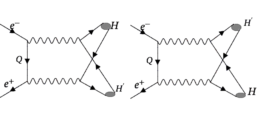
We take $P,q,\epsilon$ as the external momentum, internal momentum and the polarization vector of the outgoing axial meson $\chi_{c1}$, and $P^{\prime},q^{\prime}$ as the external and internal momenta of pseudoscalar meson, $\eta_{c}$, while $k$ and $k^{\prime}$ as the momenta of the two virtual photons involved in the process. For the two quark–rearrangement diagrams, we adopt the heavy–quark approximation used in previous charmonium studies[14], where internal relative-momentum effects are suppressed by $\sim O(v^{2})$, implying $\hat{q}^{2}/m^{2}<<1$. In this limit, the photon momenta are effectively insensitive to the internal quark motion, and the photon virtualities satisfy $k^{2}\approx k^{\prime 2}\approx s/4$. The product of the photon propagators then satisfies, $1/(k^{2}k^{\prime 2})\approx 16/s^{2}$. This is further justified since the photon virtualities are dominated by the external kinematics at $\sqrt{s}>>mv$. With this, the amplitudes for the two diagrams (Direct and Exchange) of the process $e^{-}e^{+}\rightarrow\chi_{c1}+\eta_{c}$ can be written as:

$$M_{fi}|_{D}=\frac{16e^{2}e_{Q}^{2}}{s^{2}}\left[\bar{v}_{2}\gamma_{\nu}\left(\frac{-i\not{Q}+m_{e}}{Q^{2}+m_{e}^{2}}\right)\gamma_{\mu}u_{1}\right]\int\frac{d^{4}q}{(2\pi)^{4}}\int\frac{d^{4}q^{\prime}}{(2\pi)^{4}}\text{Tr}[\gamma_{\mu}\bar{\psi}_{A}(P,q)\gamma_{\nu}\bar{\psi}_{P}(P^{\prime},q^{\prime})]$$

(5)

and

$$M_{fi}|_{X}=\frac{16e^{2}e_{Q}^{2}}{s^{2}}\left[\bar{v}_{2}\gamma_{\nu}\left(\frac{-i\not{Q}+m_{e}}{Q^{2}+m_{e}^{2}}\right)\gamma_{\mu}u_{1}\right]\int\frac{d^{4}q}{(2\pi)^{3}}\int\frac{d^{4}q^{\prime}}{(2\pi)^{4}}\text{Tr}\left[\gamma_{\mu}\bar{\psi}_{P}(P^{\prime},q^{\prime})\gamma_{\nu}\bar{\psi}_{A}(P,q)\right],\\$$

(6)

where the amplitude for the rearrangement diagram that involves the exchange of the final state mesons in the process $e^{-}e^{+}\rightarrow\chi_{c1}+\eta_{c}$ can again be obtained from the above amplitude through the exchange of Lorentz indices as ${M}^{(X)}_{fi}={M}^{(D)}_{fi}|_{\mu\leftrightarrow\nu}$. To reduce the above amplitudes to their 3D forms, we make use of the Covariant Instantaneous Ansatz (CIA), under which the 4D volume elements of the internal momenta of the two produced hadrons can be written as $d^{4}q=d^{3}\hat{q}Md\sigma$ and $d^{4}q^{\prime}=d^{3}\hat{q}^{\prime}M^{\prime}d\sigma^{\prime}$. We then integrate over the longitudinal components $Md\sigma$ and $M^{\prime}d\sigma^{\prime}$ of the internal momenta $q$ and $q^{\prime}$ of the two hadrons to obtain $\frac{1}{2\pi i}\int Md\sigma\Psi(P,q)=\bar{\Psi}(\hat{q})$ and $\frac{1}{2\pi i}\int M^{\prime}d\sigma^{\prime}\Psi(P^{\prime},q^{\prime})=\bar{\Psi}(\hat{q}^{\prime})$, which are the corresponding 3D Bethe–Salpeter wave functions used to express the full amplitudes for the process $e^{-}e^{+}\rightarrow\chi_{c1}+\eta_{c}$ in a manifestly 3D form.

Thus, for the direct amplitude of photon fragmentation diagrams, we reduce the amplitude to its 3D form as

$$M_{fi}|_{D}=\frac{16e^{2}e_{Q}^{2}}{s^{2}}\left[\bar{v}_{2}\gamma_{\nu}\left(\frac{-i\not{Q}+m_{e}}{Q^{2}+m_{e}^{2}}\right)\gamma_{\mu}u_{1}\right]\int\frac{d^{3}\hat{q}}{(2\pi)^{3}}\int\frac{d^{3}\hat{q^{\prime}}}{(2\pi)^{3}}\text{Tr}[\gamma_{\mu}\bar{\psi}_{A}(\hat{q})\gamma_{\nu}\bar{\psi}_{P}(\hat{q^{\prime}})]$$

(7)

The amplitude for the exchange process can be similarly written as:

$$M_{fi}|_{X}=\frac{16e^{2}e_{Q}^{2}}{s^{2}}\left[\bar{v}_{2}\gamma_{\nu}\left(\frac{-i\not{Q}+m_{e}}{Q^{2}+m_{e}^{2}}\right)\gamma_{\mu}u_{1}\right]\int\frac{d^{3}\hat{q}}{(2\pi)^{3}}\int\frac{d^{3}\hat{q^{\prime}}}{(2\pi)^{3}}\text{Tr}[\gamma_{\mu}\bar{\psi}_{P}(\hat{q}^{\prime})\gamma_{\nu}\bar{\psi}_{A}(\hat{q})],$$

(8)

and the 3D forms of adjoint Bethe-Salpeter wave functions of Dimensions $M$ for $\chi_{c1}$ and $\eta_{c}$ obtained by 3D reduction of the full 4D BS wave functions[39, 40] with all the Dirac structures are expressed as [21, 17]:

	$\displaystyle\bar{\psi}_{A}(\hat{q})=N_{A}\left[iM\not{\epsilon}+\not{P}\not{\epsilon}+\frac{2i\not{\hat{q}}\not{P}\not{\epsilon}}{M}\right]\gamma_{5}\phi_{A}(\hat{q}),$
	$\displaystyle\bar{\psi}_{P}(\hat{q}^{\prime})=N_{P}\gamma_{5}\left[M^{\prime}-i\not{P}^{\prime}+\frac{2\not{\hat{q}^{\prime}}\not{P}^{\prime}}{M^{\prime}}\right]\phi_{P}(\hat{q}^{\prime}).$		(9)

where the radial wave functions for $\chi_{c1}(nP)$[22] obtained through solutions of its mass spectral equation are:

	$\displaystyle\phi_{A}(\hat{q},1P)=\sqrt{\frac{2}{3}}\frac{1}{\pi^{\frac{3}{4}}\beta_{A}^{\frac{5}{2}}}\hat{q}e^{-\frac{\hat{q}^{2}}{2\beta_{A}^{2}}}$
	$\displaystyle\phi_{A}(2P,\hat{q})=\sqrt{\frac{5}{3}}\frac{1}{\pi^{\frac{3}{4}}\beta_{A}^{\frac{5}{2}}}\hat{q}(1-\frac{2}{5\beta_{A}^{2}}\hat{q}^{2})e^{-\frac{\hat{q}^{2}}{2\beta_{A}^{2}}},$		(10)

where its inverse range parameter $\beta_{A}=(\frac{2}{3}M\omega_{q\bar{q}}^{2})^{1/4}$ [17] is derived from the mass spectral equation for $\chi_{c1}(nP)$, with $\omega_{q\bar{q}}^{2}=M\omega_{0}^{2}\alpha_{s}(M^{2})$[21, 14] being the flavour dependent spring constant. The corresponding radial wave functions for $\eta_{c}(nS)$[21] are:

	$\displaystyle\phi_{P}(\hat{q},1S)=\frac{1}{\pi^{\frac{3}{4}}\beta_{P}^{\frac{3}{2}}}e^{-\frac{\hat{q}^{2}}{2\beta_{P}^{2}}}$
	$\displaystyle\phi_{P}(\hat{q},2S)=\sqrt{\frac{3}{2}}\frac{1}{\pi^{\frac{3}{4}}\beta_{P}^{\frac{3}{2}}}(1-\frac{2}{3\beta_{P}^{2}}\hat{q}^{2})e^{-\frac{\hat{q}^{2}}{2\beta_{P}^{2}}}.$		(11)

where its inverse range parameter is: $\beta_{P}=(M\omega_{q\bar{q}}^{2})^{1/4}$[17, 21]. And $N_{A}$, and $N_{P}$ are the 4D BS normalizers that are obtained through the current conservation condition,

$$2iP_{\mu}=\int\frac{d^{4}q}{(2\pi)^{4}}\mbox{Tr}\left\{\overline{\Psi}(P,q)\left[\frac{\partial}{\partial P_{\mu}}S_{F}^{-1}(p_{1})\right]\Psi(P,q)S_{F}^{-1}(-p_{2})\right\}+(1\rightleftharpoons 2),$$

(12)

where, $\Psi(P,q)$ is the 4D BS wave function, while $\overline{\Psi}(P,q)=\gamma_{4}\Psi(P,q)^{{\dagger}}\gamma_{4}$ is the adjoint BS wave function. The above equation is reduced to 3D form by integrating the RHS over the longitudinal component $Md\sigma$, which reduces $\Psi_{A}(P,q)$ (and $\bar{\Psi}_{P}(P,q)$) to their 3D forms $\psi_{A}(\hat{q})$ (and $\bar{\psi}_{P}(P,q)$), whose algebraic forms are in Eqs.(9). Evaluating the trace over the gamma matrices, and multiplying both sides by $P_{\mu}/(-M^{2})$, we then extract the BS normalizers:

	$\displaystyle N_{A}^{-2}=\frac{4M^{2}}{m}\int\frac{d^{3}\hat{q}}{(2\pi)^{3}}\phi_{A}^{2}(\hat{q}),$
	$\displaystyle N_{P}^{-2}=\frac{16M}{m}\int\frac{d^{3}\hat{q}}{(2\pi)^{3}}\frac{\hat{q}^{2}}{\omega}\phi_{P}^{2}(\hat{q}).$		(13)

whose numerical values for $N_{A}$ and $N_{P}$ for the process studied are listed in table 2. The total amplitude $M_{fi}$ after trace evaluation over the gamma matrices, and making use of the fact that $P^{\prime}.\epsilon=0$ in the center of mass frame, can be written as:

	$\displaystyle M_{fi}|_{D}=N_{P}N_{A}\frac{16e^{2}e_{Q}^{2}}{s^{2}}\int\frac{d^{3}\hat{q}}{(2\pi)^{3}}\phi_{A}(\hat{q})\int\frac{d^{3}\hat{q}^{\prime}}{(2\pi)^{3}}\phi_{P}(\hat{q^{\prime}})\Big\{4M^{\prime}\Big[\bar{v}_{2}\not{\epsilon}\Big(\frac{-i\not{Q}+m_{e}}{Q^{2}+m_{e}^{2}}\Big)\not{P}u_{1}\Big]$
	$\displaystyle\qquad-4M^{\prime}\Big[\bar{v}_{2}\not{P}\Big(\frac{-i\not{Q}+m_{e}}{Q^{2}+m_{e}^{2}}\Big)\not{\epsilon}u_{1}\Big]+4M\Big[\bar{v}_{2}\not{P^{\prime}}\Big(\frac{-i\not{Q}+m_{e}}{Q^{2}+m_{e}^{2}}\Big)\not{\epsilon}u_{1}\Big]+4M\Big[\bar{v}_{2}\not{\epsilon}\Big(\frac{-i\not{Q}+m_{e}}{Q^{2}+m_{e}^{2}}\Big)\not{P^{\prime}}u_{1}\Big]\Big\}$

The above expression can be further compactified by introducing $G_{1}$ (for axial vector meson $\chi_{c1}$), and $G_{2}$ (for pseudoscalar meson $\eta_{c}$) as 3D integrals involving the two outgoing mesons, defined as:

	$\displaystyle G_{1}=\int\frac{d^{3}\hat{q}}{(2\pi)^{3}}\phi_{A}(\hat{q})$
	$\displaystyle G_{2}=\int\frac{d^{3}\hat{q}^{\prime}}{(2\pi)^{3}}\phi_{P}(\hat{q}^{\prime}),$		(15)

where in the above integrals, the unnormalized forms of the 3D radial wave functions $\phi_{A}(\hat{q})$ and $\phi_{P}(\hat{q})$ are taken from Eqs. (10-11), since to calculate the transition amplitude, $M_{fi}$, we use the 4D BS normalizers $N_{A}$ and $N_{P}$ that are obtained through the covariant current condition Eq.(12). The 4D BS normalizer already encodes the full normalization of the bound-state wave function. Imposing an additional 3D normalization on $\phi_{A}$ and $\phi_{P}$ would therefore constitute a double-counting of the wave function normalization. This is consistent with the normalization convention adopted throughout the present work and in our earlier studies [24, 23, 16, 17, 14, 18].

Further here, we have made use of the fact that $\hat{q}$ is an effective 3D variable and is a directional vector, due to which all terms in Trace with $\hat{q}$ become zero after the 3D integration over $d^{3}\hat{q}$. Further the terms involving $P^{\prime}.\epsilon$ vanish. This is due to the fact that $P.\epsilon=\overrightarrow{P}.\overrightarrow{\epsilon}=0$, since momentum, $P=(\overrightarrow{P},iE)$ of axial meson is always orthogonal to its polarization vector, $\epsilon=(\overrightarrow{\epsilon},i0)$. And in center of mass frame, $\overrightarrow{P}^{\prime}=-\overrightarrow{P}$, which implies that $\overrightarrow{P}^{\prime}.\overrightarrow{\epsilon}=P^{\prime}.\epsilon=0$.

The first and second term contributes equally in the $|M_{fi}|^{2}$ and the same is true as regards the third term and fourth term in Eq.(14). The Direct amplitude can then be written as:

	$\displaystyle M_{fi}|_{D}=N_{P}N_{A}\frac{16e^{2}e_{Q}^{2}}{s^{2}}G_{1}G_{2}\Big\{4M^{\prime}\Big[\bar{v}_{2}\not{\epsilon}\Big(\frac{-i\not{Q}+m_{e}}{Q^{2}+m_{e}^{2}}\Big)\not{P}u_{1}\Big]-4M^{\prime}\Big[\bar{v}_{2}\not{P}\Big(\frac{-i\not{Q}+m_{e}}{Q^{2}+m_{e}^{2}}\Big)\not{\epsilon}u_{1}\Big]$
	$\displaystyle~~~~~~~~~~~~~~~~~~~~~~~~~~~~~~~~~~~~~~~~~~~~~+4M\Big[\bar{v}_{2}\not{P^{\prime}}\Big(\frac{-i\not{Q}+m_{e}}{Q^{2}+m_{e}^{2}}\Big)\not{\epsilon}u_{1}\Big]+4M\Big[\bar{v}_{2}\not{\epsilon}\Big(\frac{-i\not{Q}+m_{e}}{Q^{2}+m_{e}^{2}}\Big)\not{P^{\prime}}u_{1}\Big]\Big\},$		(16)

while the exchange amplitude with the final states interchanged is:

	$\displaystyle M_{fi}|_{X}=N_{P}N_{A}\frac{16e^{2}e_{Q}^{2}}{s^{2}}G_{1}G_{2}\Big\{-4M^{\prime}\Big[\bar{v}_{2}\not{\epsilon}\Big(\frac{-i\not{Q}+m_{e}}{Q^{2}+m_{e}^{2}}\Big)\not{P}u_{1}\Big]+4M^{\prime}\Big[\bar{v}_{2}\not{P}\Big(\frac{-i\not{Q}+m_{e}}{Q^{2}+m_{e}^{2}}\Big)\not{\epsilon}u_{1}\Big]$
	$\displaystyle~~~~~~~~~~~~~~~~~~~~~~~~~~~~~~~~~~~~~~~~~~~~~+4M\Big[\bar{v}_{2}\not{P^{\prime}}\Big(\frac{-i\not{Q}+m_{e}}{Q^{2}+m_{e}^{2}}\Big)\not{\epsilon}u_{1}\Big]+4M\Big[\bar{v}_{2}\not{\epsilon}\Big(\frac{-i\not{Q}+m_{e}}{Q^{2}+m_{e}^{2}}\Big)\not{P^{\prime}}u_{1}\Big]\Big\}.$		(17)

The total amplitude would then be: $M_{fi}=M_{fi}|_{D}+M_{fi}|_{X}$ is written as:

$$M_{fi}=N_{P}N_{A}\frac{16e^{2}e_{Q}^{2}}{s^{2}}G_{1}G_{2}\Bigg(8M\Big[\bar{v}_{2}\not{P^{\prime}}\Big(\frac{-i\not{Q}+m_{e}}{Q^{2}+m_{e}^{2}}\Big)\not{\epsilon}u_{1}\Big]+8M\Big[\bar{v}_{2}\not{\epsilon}\Big(\frac{-i\not{Q}+m_{e}}{Q^{2}+m_{e}^{2}}\Big)\not{P^{\prime}}u_{1}\Big]\Bigg).$$

(18)

We now evaluate the spin averaged invariant amplitude modulus squared, $|\bar{M}_{fi}|^{2}=\frac{1}{4}\sum_{s1,s2,\lambda}{M^{\dagger}}_{fi}M_{fi}$, for which we must now average over the initial spin states of $e^{-}$ and $e^{+}$ and sum over the polarisation states of the final axial vector meson $\chi_{c1}$. We make use of the normalization relation, $\Sigma_{\lambda}\epsilon_{\mu}^{\lambda}\epsilon_{\nu}^{\lambda}=\frac{1}{3}(\delta_{\mu\nu}+\frac{P_{\mu}P_{\nu}}{M^{2}})$ ¹¹1We have made use of the ”Euclidean” notation-treating time part as the fourth component of a four-vector, where our metric is $\delta_{\mu\nu}$ for the polarisation vector of the axial meson.

As regards the kinematics of the process is concerned, one can note that $\overline{p}_{1}+\overline{p}_{2}=k+k^{\prime}=P+P^{\prime}$. Also, since $k=\overline{p}_{1}-Q$, and $k^{\prime}=Q+\overline{p}_{2}$, we can obtain the momentum relation, $\bar{p}_{1}-\bar{p}_{2}=2Q+k-k^{\prime}\approx 2Q$. And in center of mass frame, where $\bar{p}_{1}=(\overrightarrow{p},iE)$, and $\bar{p}_{2}=(-\overrightarrow{p},iE)$, we can write, $Q=(\overrightarrow{p},i0)$. Thus we can obtain,

$$Q^{2}=-{m_{e}}^{2}+\frac{s}{4}.$$

(19)

Taking $\theta$ to be the angle between the incident beam direction and $\chi_{c1}$ (or $h_{c}$ in Section 4), the dot products of various momenta in the center of mass frame can be expressed as:  $\bar{p_{1}}.\bar{p_{2}}=-\frac{s}{2}$,  $\bar{p}_{1}.P=-\frac{s}{4}(1+Cos\theta)=\bar{p}_{2}.P^{\prime}$,   $\bar{p}_{1}.P^{\prime}=\frac{s}{4}(-1+Cos\theta)=\bar{p}_{2}.P$,  $Q.P=\frac{s}{4}Cos\theta$,    $Q.P^{\prime}=-\frac{s}{4}Cos\theta$. Similarly, $\bar{p_{1}}.Q=-\bar{p_{2}}.Q\sim\frac{s}{4}$,   $P.P^{\prime}=-\frac{s}{2}+M^{2}$,   $P.I=0$,   $P^{\prime}.I=0$. And $P.\epsilon=P^{\prime}.\epsilon^{\prime}=0$,    $P.\epsilon^{\prime}=P^{\prime}.\epsilon=0$. Similarly, the dot products: $p_{1}.I=p_{2}.I^{\prime}=\frac{\sqrt{s}}{2}Sin\theta$,   $p_{1}.I^{\prime}=p_{2}.I=-\frac{\sqrt{s}}{2}Sin\theta$,    $I.Q=\frac{\sqrt{s}}{2}Sin\theta$, and $I^{\prime}.Q=-\frac{\sqrt{s}}{2}Sin\theta$. Here $I=\frac{\hat{q}}{|\hat{q}|}$, and $I^{\prime}=\frac{\hat{q}^{\prime}}{|\hat{q}^{\prime}|}$ are unit vectors along the direction of $\hat{q}$ and $\hat{q}^{\prime}$ respectively, while $|\hat{q}|=\sqrt{q^{2}-\frac{(q.P)^{2}}{P^{2}}}$ and $|\hat{q}^{\prime}|=\sqrt{{q^{\prime}}^{2}-\frac{(q^{\prime}.P^{\prime})^{2}}{P^{\prime 2}}}$ are Lorentz-invariant variables. Also, $(\bar{p_{1}}+\bar{p_{2}})^{2}=-s$. These kinematical relations are valid for the quark rearrangement diagrams applicable for these transitions. We obtain

	$\displaystyle\left|\mathcal{M}_{fi}\right|^{2}$	$\displaystyle=$	$\displaystyle\frac{e^{4}\,e_{Q}^{4}\cdot 16^{2}\,G_{1}^{2}\,G_{1}^{\prime\,2}}{24\,s^{4}\left(Q^{2}+m_{e}^{2}\right)^{2}}\Bigg[-\cos^{4}\theta\left(s_{1}^{2}-4M^{2}\right)^{2}\left(s_{1}^{2}-4m_{e}^{2}\right)^{2}$		(20)
			$\displaystyle+\;\cos^{2}\theta\;s_{1}^{2}\left(s_{1}^{2}-2M_{p}^{2}\right)\left(s_{1}^{2}-4M^{2}\right)\left(s_{1}^{2}-4m_{e}^{2}\right)$
			$\displaystyle+\;M^{2}\Bigg(-\cos^{3}\theta\left(s_{1}^{2}-4M^{2}\right)^{3/2}\left(s_{1}^{2}-4m_{e}^{2}\right)^{3/2}$
			$\displaystyle\hskip 18.49988pt+\;2\cos^{2}\theta\;s_{1}^{2}\sqrt{s_{1}^{2}-4M^{2}}\left(s_{1}^{2}-4m_{e}^{2}\right)\sqrt{s_{1}^{2}-4M_{p}^{2}}$
			$\displaystyle\hskip 18.49988pt+\;12\,m_{e}^{2}\cos^{2}\theta\left(s_{1}^{2}-4M^{2}\right)\left(s_{1}^{2}-4m_{e}^{2}\right)$
			$\displaystyle\hskip 18.49988pt-\;2\cos\theta\;s_{1}^{2}\left(s_{1}^{2}-2m_{e}^{2}\right)\sqrt{\left(s_{1}^{2}-4M^{2}\right)\left(s_{1}^{2}-4m_{e}^{2}\right)}$
			$\displaystyle\hskip 18.49988pt+\;s_{1}^{2}\left(s_{1}^{2}-4m_{e}^{2}\right)\left(s_{1}^{2}-4M_{p}^{2}\right)\Bigg)\Bigg]$

Here $\alpha=\frac{e^{2}}{4\pi}$ is the QED coupling constant, while, $N_{A}$ and $N_{P}$ are the BS normalizers of axial and pseudoscalar mesons and are evaluated through the current conservation condition, Eq.(12). The total cross section for the process is given as,

$$\sigma=\frac{1}{32\pi^{2}s^{3/2}}|\vec{P^{\prime}}|\int d\Omega^{\prime}|\bar{M}_{fi}|^{2},$$

(21)

with $|\vec{P^{\prime}}|=\sqrt{\frac{1}{s}[s-(M+M^{\prime})^{2}][s-(M-M^{\prime})^{2}]}$ being the momenta of either of the final particles. It is observed that the dimensions of the following quantities are as follows: $G_{1}\sim M^{4}$, $G_{2}\sim M^{3}$, $N_{A}\sim M^{-3}$, $N_{P}\sim M^{-2}$, $|\bar{M}_{fi}|^{2}\sim M^{0}$, due to which the cross section, $\sigma\sim M^{-2}$. The numerical values of cross sections for $e^{-}e^{+}\rightarrow\chi_{c1}(nP)+\eta_{c}(nS)$ (with n=1,2) in our work at $\sqrt{s}$=10.6 GeV along with the results of NRQCD[4] are given in Table 1.

References

- [1] K. Abe et al.(Belle), Phys. Rev. Lett. 89, 142001 (2002);[hep-ex/0205104].
- [2] K. Abe et al.(Belle), Phys. Rev. D 70, 071102 (2004); [hep-ex/0407009].
- [3] B. Aubert et al.(BABAR),Phys. Rev. D 72, 031101(2005); [hep-ex/0506062].
- [4] G. T. Bodwin, J. Lee, and E. Braaten, Phys. Rev. D 67, 054023(2003), [hep-ph/0212352].[Erratum: Phys.Rev.D 72, 099904 (2005)].
- [5] G.T. Bodwin, E. Braaten, G.P. Lepage, Phys. Rev. D 51 (1995) 1125, Phys. Rev. D 55 (1997) 5853.
- [6] G. T. Bodwin, J. Lee, and E. Braaten, Phys. Rev. Lett.90. 162001(2003), [hep-ph/0212181].
- [7] G. T. Bodwin, E. Braaten, J. Lee, and C. Yu, Phys. Rev. D 74, 074014(2006), [hep-ph/0608200].
- [8] B. Gong and J.-X. Wang, Phys. Rev. Lett. 100, 181803(2008), [arXiv:0801.0648].
- [9] X-D Huang, B. Gong, R-C Niu, H-M Yu, J-X Wang, JHEP 02, 055 (2024); arxiv: 2311.04751[hep-ph].
- [10] Y.Fan, J.Lee, C.Yu, Phys. Rev. D 87, 094032 (2013); arxiv:1211.4111[hep-ph].
- [11] E.Braaten, J. Lee, Phys. Rev. D67, 054007,(2003).
- [12] A.V.Luchinsky,Phys. Atom. Nucl. 67, 1338 (2004); hep-ph/0301190.
- [13] M. Davier, M. E. Peskin, and A. Snyder, hep-ph/0606155.
- [14] S.Bhatnagar, H.Negash, Nucl. Phys. A1053, 122969 (2025).
- [15] V.V.Braguta, Phys. Rev. D78, 054025 (2008); arxiv:0712.1475[hep-ph].
- [16] S.Bhatnagar, V.Guleria, Nucl. Phys. A1041, 122783(2024).
- [17] M.Narang, S.Bhatnagar, Few-Body Systs. 64, 82(2023).
- [18] S.Bhatnagar, Phys. Rev. D112, 054011 (2025).
- [19] S.Bhatnagar, L.Alemu, Phys. Rev. D97, 034021 (2018).
- [20] V.Guleria, E.Gebrehana, S.Bhatnagar, Pramana J. Physics 99, 169 (2025).
- [21] E.Gebrehana, S.Bhatnagar, H.Negash, Phys. Rev. D100, 054034 (2019).
- [22] V.Guleria, S.Bhatnagar, Intl. J. Theor. Phys. 60, 3143 (2021).
- [23] V.Guleria, E.Gebrehana, S.Bhatnagar, Phys. Rev. D104, 094045 (2021).
- [24] S.Bhatnagar, E.Gebrehana, Phys. Rev. D102, 094024 (2020).
- [25] A.N.Mitra, S.Bhatnagar, Intl. J. Mod. Phys. A07, 121 (1992).
- [26] T. Wang, Y. Jiang, W.L. Ju, H. Yuan, G.L. Wang, J. High Energy Phys. 03, 209 (2016).
- [27] J.K. He, Eur. Phys. J. C 79, 393 (2019)
- [28] J.K. He, C.J. Fan, Phys. Rev. D 103, 114006 (2021).
- [29] Z.H.Wang, G.L.Wang, Phys. Rev. D106, 054037 (2022).
- [30] H.Negash, S.Bhatnagar, Intl. J. Mod. Phys. E25, 1650059 (2016).
- [31] M.S. Bhagwat, A. Krassnigg, P. Maris, C.D. Roberts, arXiv :nucl -th /0612027.
- [32] A. Bender, C.D. Roberts, L.V. Smekal, Phys. Lett. B 380 (1996) 7
- [33] P. Maris, A. Raya, C.D. Roberts, S.M. Schmidt, Eur. Phys. J. A 18 (2003) 231;
- [34] P. Maris, C.D. Roberts, Int. J. Mod. Phys. E 12 (2003) 297.
- [35] B. El-Bennich, M.A. Ivanov, C.D. Roberts, Phys. Rev. C 83 (2011) 025205.
- [36] C.H. Chang, J.X. Wang, X.G. Wu, Sci. China, Phys. Mech. Astron. 53 (2010) 2031, arXiv :1005 .4723 [hep -ph].
- [37] Z.G. Wang, W.M. Yang, S.L. Wan, Phys. Lett. B 615 (2005) 75, arXiv :hep -ph /0411142.
- [38] J. Yi, S-Y. Li, Y-R. Liu, Z-X. Meng, Z-G. Si, T. Yao, Phys. Rev. C 102 (2020) 015201.
- [39] C.H.L.Smith, Ann. Phys. (N.Y.) 53, 521 (1969).
- [40] R. Alkofer and L. V. Smekel, Phys. Rep. 353, 281 (2002).
- [41] Q-L.Liao, Y. Yu, Eur. Phys. J. C84, 1000 (2024).
- [42] Q.L. Liao, J. Jiang, Y.H. Zhao, Eur. Phys. J. C83, 22 (2022).