The disjoint separators problem in graphs

Consider a red-blue coloring of the non-terminal vertices in $G$. Since $(G_{0},S_{r},T_{r},S_{b},T_{b})$ is a NO-instance, the subgraph induced by $G_{0}$ contains a red path between $S_{r}$ and $T_{r}$ or a blue path between $S_{b}$ and $T_{b}$. Hence, $G$ also contains such a path. ∎

Assume that $\textup{dist}_{G}(S_{r},S_{b})\geq 3$ (the other cases are analogous). Then, we color the non-terminal vertices that are neighbors of a red source in blue, and the other non-terminal vertices in red. In this way, all neighbors of red sources are colored in blue, and, since $\textup{dist}_{G}(S_{r},S_{b})\geq 3$, all neighbors of blue sources are colored in red. This clearly ensures that there is no monochromatic path between a source and a target of the same color. ∎

Let $(G,S_{r},T_{r},S_{b},T_{b})$ be an instance of GeneralDisjointSeparators. Let $G_{0}$ be the graph obtained from $G$ by adding four new vertices $s_{r},t_{r},s_{b},t_{b}$ and adding: all edges between $\{s_{r}\}$ and $S_{r}\cup S_{b}\cup T_{b}$, all edges between $\{t_{r}\}$ and $T_{r}\cup S_{b}\cup T_{b}$, all edges between $\{s_{b}\}$ and $S_{b}\cup S_{r}\cup T_{r}$, and all edges between $\{t_{b}\}$ and $T_{b}\cup S_{r}\cup T_{r}$. We claim that the instances $(G_{0},s_{r},t_{r},s_{b},t_{b})$ and $(G,S_{r},T_{r},S_{b},T_{b})$ are equivalent. Indeed, in the former instance, every vertex $u\in S_{r}\cup T_{r}$ must be colored in red because of the path $s_{b}ut_{b}$, and every vertex $v\in S_{b}\cup T_{b}$ must be colored in blue because of the path $s_{r}vt_{r}$. From there, the existence of a red path between $s_{r}$ and $t_{r}$ (resp. between $s_{b}$ and $t_{b}$) is equivalent to the existence of a red path between $S_{r}$ and $T_{r}$ (resp. between $S_{b}$ and $T_{b}$). ∎

Note that the non-terminal vertices are the same for both instances. Given a red-blue coloring of the non-terminal vertices, we clearly have a red path between $w$ and some vertex in $T_{r}$ in the second instance if and only if we have a red path between $u$ or $v$ and some vertex in $T_{r}$ in the first instance. ∎

Consider an instance $(G,s_{r},t_{r},s_{b},t_{b})$. Recall that, by 1.1, $s_{r}$ and $t_{r}$ are not adjacent, and neither are $s_{b}$ and $t_{b}$.

Let us note that, if $s_{r}$, $t_{r}$, $s_{b}$ and $t_{b}$ do not all belong to the same connected component of $G$, then we have a YES-instance: indeed, for each connected component $C$, simply give all the non-terminal vertices of $C$ the same color, blue if $\{s_{r},t_{r}\}\subseteq C$ or red otherwise.

Therefore, we may assume that $G$ is connected, by only considering the connected component containing $s_{r}$, $t_{r}$, $s_{b}$ and $t_{b}$. We now explain how to eliminate each cut vertex in linear time, so that we get a 2-connected graph in quadratic time. Let $v$ be a cut vertex of $G$, and note that finding $v$ and computing the connected components of $G-v$ can easily be done in linear time.

First, suppose that $v\in\{s_{r},t_{r},s_{b},t_{b}\}$. Without loss of generality, assume $v=s_{r}$. Let $C$ be the connected component of $G-s_{r}$ that contains $t_{r}$. If $\{s_{b},t_{b}\}\subseteq C$, then $(G[C\cup\{s_{r}\}],s_{r},t_{r},s_{b},t_{b})$ is an equivalent instance. If $\{s_{b},t_{b}\}\not\subseteq C$, then we have a YES-instance: simply color the non-terminal vertices of $C$ in blue and the other non-terminal vertices in red.

We now suppose that $v\not\in\{s_{r},t_{r},s_{b},t_{b}\}$. For $x\in\{s_{r},t_{r},s_{b},t_{b}\}$, let $C(x)$ be the connected component of $G-v$ that contains $x$. Using the symmetries, we only need to consider the following four cases, with Figure 2 providing some illustrations.

1. 1)

   First case: $C(s_{r})=C(t_{r})=C(s_{b})=C(t_{b})$.

   Clearly, $(G[C(s_{r})\cup\{v\}],s_{r},t_{r},s_{b},t_{b})$ is an equivalent instance. Note that we are always in this case if $s_{r}s_{b}t_{r}t_{b}$ is a cycle, so we do keep the same four terminals in that case as required by the statement of this proposition.

2. 2)

   Second case: $C(s_{r})\neq C(t_{r})$, and $C(s_{b})\neq C(t_{b})$.

   If $s_{r}$, $t_{r}$, $s_{b}$ and $t_{b}$ are all neighbors of $v$ in $G$, then we obviously have a NO-instance since there will be either a red path $s_{r}vt_{r}$ or a blue path $s_{b}vt_{b}$. Otherwise, we have a YES-instance: indeed, if $s_{r}$ or $t_{r}$ (resp. $s_{b}$ or $t_{b}$) is not a neighbor of $v$, simply color $v$ in red (resp. blue) and the other non-terminal vertices in blue (resp. red).

3. 3)

   Third case: $C(s_{r})=C(t_{r})$, $C(s_{b})\neq C(s_{r})$, and $C(t_{b})\neq C(s_{r})$.

   Again, we assume that $s_{r}$, $t_{r}$, $s_{b}$ and $t_{b}$ are not all neighbors of $v$ in $G$. We then have a YES-instance. Indeed, if $s_{r}$ or $t_{r}$ is not a neighbor of $v$, then color all the non-terminal vertices of $C(s_{r})$ in blue and the other non-terminal vertices (this includes $v$) in red. Otherwise, if $s_{b}$ (resp. $t_{b}$) is not a neighbor of $v$, then color all the non-terminal vertices of $C(s_{b})$ (resp. $C(t_{b})$) in red and the other non-terminal vertices (this includes $v$) in blue.

4. 4)

   Fourth case: $C(s_{r})=C(t_{r})=C(t_{b})$, and $C(s_{b})\neq C(t_{b})$.

   Again, we assume that $s_{r}$, $t_{r}$, $s_{b}$ and $t_{b}$ are not all neighbors of $v$ in $G$.

   1. a)

      If either $s_{r}$ or $t_{r}$ is not a neighbor of $v$, then we have a YES-instance: simply color $v$ in red and the other non-terminal vertices in blue.

   2. b)

      If $s_{b}$ is not a neighbor of $v$, then we also have a YES-instance: color all non-terminal vertices of $C(s_{b})$ in red and the other non-terminal vertices (this includes $v$) in blue.

   3. c)

      Finally, suppose that $s_{r}$, $t_{r}$ and $s_{b}$ are neighbors of $v$, but $t_{b}$ is not. Since $s_{r}$ and $t_{r}$ are neighbors of $v$, coloring $v$ in blue is forced. Since $s_{b}$ is a neighbor of $v$, for any coloring in which $v$ is blue, there is a blue $s_{b}t_{b}$-path in $G$ if and only if there is a blue $vt_{b}$-path in $G[C(t_{b})\cup\{v\}]$. Therefore, $(G[C(t_{b})\cup\{v\}],s_{r},t_{r},v,t_{b})$ is an equivalent instance. ∎

We assume that $C$ is the outer face and that all inner faces are triangles. Indeed, by our assumption on $G$, we could reduce to that case by removing all vertices strictly outside $C$ and all vertices strictly inside remaining triangles, and then conclude using 2.1.

Fix a red-blue coloring of the non-terminal vertices. We want to show that there exists a red $s_{r}t_{r}$-path or a blue $s_{b}t_{b}$-path. For this, we use Gale’s algorithm [5], which builds a walk in the dual graph of $G$ (Figure 10 provides an illustration, on the instance from Figure 9(a) where we have removed the two vertices that were strictly inside a triangle). An edge of $G$ is called mixed if its endpoints have different colors. We define two finite sequences $(r_{i})_{i}$ and $(b_{i})_{i}$ of red and blue vertices respectively, as follows. We set $r_{0}=s_{r}$ and $b_{0}=s_{b}$. We start on the outer face, and we “enter” the graph through the mixed edge $s_{r}s_{b}=r_{0}b_{0}$. From there, any time we enter an inner face $r_{i}b_{i}v$ through the mixed edge $r_{i}b_{i}$, we exit it through its only other mixed edge. If that edge is $r_{i}v$, i.e., $v$ is blue, then we define $r_{i+1}=r_{i}$ and $b_{i+1}=v$. Otherwise, we define $r_{i+1}=v$ and $b_{i+1}=b_{i}$. An inner face that has been visited once will never be visited again, since both its mixed edges have been used. Therefore, at some point, we enter the outer face again through some mixed edge $r_{k}b_{k}$: when this happens, the algorithm stops.

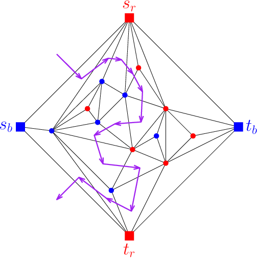
We know that $(r_{k},b_{k})\in\{(s_{r},t_{b}),(t_{r},s_{b}),(t_{r},t_{b})\}$. As a side note, it is actually impossible that $(r_{k},b_{k})=(t_{r},t_{b})$, since we always go through a mixed edge with its red vertex to our left and its blue vertex to our right. In all cases, we have $r_{k}=t_{r}$ or $b_{k}=t_{b}$. If $r_{k}=t_{r}$ then, since $r_{i+1}$ either equals $r_{i}$ or is a neighbor of $r_{i}$ by construction, the sequence $(s_{r}=r_{0},r_{1}\ldots,r_{k}=t_{r})$ contains a red $s_{r}t_{r}$-path. If $b_{k}=t_{b}$ then, similarly, the sequence $(s_{b}=b_{0},b_{1}\ldots,b_{k}=t_{b})$ contains a blue $s_{b}t_{b}$-path. ∎

The 3-connectivity of $G^{\phi}$ is straightforward, since it clearly contains a triangulation of $G$ as a spanning subgraph, and all triangulations are 3-connected [3, 7]. However, the second part of the lemma cannot be obtained as easily, as triangulating $G$ may create a triangle $(s,t)$-separator, preventing us from using the aforementioned 4-connectivity result for triangulations (actually, it can be easily seen that the equivalence would be false if $G^{\phi}$ was replaced by a triangulation of $G$).

Let $s,t\in V$ be distinct. It is clear that $(iii)$$\implies$$(ii)$. Moreover, we also have $(i)$$\implies$$(iii)$: indeed, a triangle $(s,t)$-separator in $G$ would also be an $(s,t)$-separator in $G^{\phi}$, so by Menger’s theorem it would imply that there do not exist four pairwise internally-vertex-disjoint $st$-paths in $G^{\phi}$. Therefore, it only remains to show that $(ii)$$\implies$$(i)$.

Suppose that there is no triangle $T$ in $G$ such that, for $\phi$, one of $s$ or $t$ is strictly inside $T$ and the other is strictly outside $T$. We proceed by contradiction and assume that there do not exist four pairwise internally-vertex-disjoint $st$-paths in $G^{\phi}$. By Menger’s theorem, this means there exists an $(s,t)$-separator $\{x_{1},x_{2},x_{3}\}$ in $G^{\phi}$. Also by Menger’s theorem, since $G$ is 2-connected, there exist two internally-vertex-disjoint $st$-paths $P_{1}=u_{0}u_{1}\ldots u_{k}$ and $P_{2}=v_{0}v_{1}\ldots v_{\ell}$ in $G$, where $u_{0}=v_{0}=s$ and $u_{k}=v_{\ell}=t$. If $P_{1}$ or $P_{2}$ contains neither $x_{1}$, $x_{2}$ nor $x_{3}$, then that path is an $st$-path in $G$ (and in $G^{\phi}$) that avoids the separator $\{x_{1},x_{2},x_{3}\}$, so we already have our contradiction. Therefore, up to some re-indexing, assume that $P_{1}$ contains $x_{1}$ but not $x_{2}$ nor $x_{3}$, and that $P_{2}$ contains at least one of $x_{2}$ or $x_{3}$. Define $i\in\{1,\ldots,k-1\}$ as the unique index such that $x_{1}=u_{i}$.

The key observation is that, for every $x\in V$, $G^{\phi}[N_{G}[x]]$ contains a spanning wheel centered at $x$ (see $x_{1}$ in Figure 12 for example). Indeed, if $y_{0},\ldots,y_{|N_{G}(x)|-1}$ is a clockwise list of the neighbors of $x$ in $G$, then $y_{j}$ and $y_{j+1}$ (where the indices are taken modulo $|N_{G}(x)|$) sit on a common face of $G$, so they are adjacent in $G^{\phi}$. This wheel can then be used to get around $x$ if we want to build a path that avoids $x$. We will use this method to build an $st$-path in $G^{\phi}$ that avoids $x_{1}$, $x_{2}$ and $x_{3}$, hence the contradiction.

Let $C$ be the cycle formed by the paths $P_{1}$ and $P_{2}$. Let $w_{0},w_{1},\ldots,w_{p}$ be the neighbors of $x_{1}=u_{i}$ in $G$ whose incident edges to $x_{1}$ lie inside $C$, listed in the order encountered along $\phi$ from $w_{0}=u_{i-1}$ to $w_{p}=u_{i+1}$. Similarly, let $w^{\prime}_{0},w^{\prime}_{1},\ldots,w^{\prime}_{p^{\prime}}$ be the neighbors of $x_{1}=u_{i}$ in $G$ whose incident edges to $x_{1}$ lie outside $C$, listed in the order encountered along $\phi$ from $w^{\prime}_{0}=u_{i-1}$ to $w^{\prime}_{p^{\prime}}=u_{i+1}$. See Figure 12.

We already know that $\{u_{0},\ldots,u_{i-1},u_{i+1},\ldots,u_{k}\}\cap\{x_{2},x_{3}\}=\varnothing$. If $\{w_{1},\ldots,w_{p-1}\}\cap\{x_{2},x_{3}\}=\varnothing$, then the sequence $(u_{0},u_{1},\ldots,u_{i-1},w_{1},\ldots,w_{p-1},u_{i+1},\ldots,u_{k})$, which is an $st$-walk in $G^{\phi}$, avoids $x_{1}$, $x_{2}$ and $x_{3}$: this is a contradiction. Similarly, if $\{w^{\prime}_{1},\ldots,w^{\prime}_{p^{\prime}-1}\}\cap\{x_{2},x_{3}\}=\varnothing$, then the $st$-walk $(u_{0},u_{1},\ldots,u_{i-1},w^{\prime}_{1},\ldots,w^{\prime}_{p^{\prime}-1},u_{i+1},\ldots,u_{k})$ avoids $x_{1}$, $x_{2}$ and $x_{3}$: since this $st$-walk contains an $st$-path, we get a a contradiction.

References

- [1] (1985) A linear algorithm for embedding planar graphs using pq-trees. Journal of Computer and System Sciences 30 (1), pp. 54–76. External Links: Document Cited by: §4.2.
- [2] (1985) Arboricity and subgraph listing algorithms. SIAM Journal on Computing 14 (1), pp. 210–223. External Links: Document Cited by: §4.2.
- [3] (2017) Graph theory. Fifth edition, Graduate Texts in Mathematics, Vol. 173, Springer, Berlin. External Links: ISBN 978-3-662-53621-6, Document, Link, MathReview Entry Cited by: §4.1, §4.1.
- [4] (1976) A combinatorial problem which is complete in polynomial space. Journal of the ACM 23 (4), pp. 710–719. External Links: Document Cited by: §1.1.
- [5] (1979) The game of Hex and the Brouwer fixed-point theorem. American Mathematical Monthly 86 (10), pp. 818–827. External Links: ISSN 0002-9890,1930-0972, Document, Link, MathReview (Aviezri S. Fraenkel) Cited by: §4.1, §4.1.
- [6] (2025) A unified convention for achievement positional games (extended abstract). EuroComb’25: 13th European Conference on Combinatorics, Graph Theory and Applications, 25-29 August 2025, Budapest, Hungary. Note: Cited by: §1.1.
- [7] (1978) On the connectivity of maximal planar graphs. Journal of Graph Theory 2 (4), pp. 307–314. External Links: ISSN 0364-9024,1097-0118, Document, Link, MathReview (D. J. Kleitman) Cited by: §4.1, §4.1.
- [8] (2014) Positional Games. Vol. 44, Springer. External Links: Document Cited by: §1.1.
- [9] (26 December 1942) Vil de laere Polygon? (in Danish). Politiken. Note: JP/Politikens Hus A/S, Copenhagen, Denmark Cited by: §1.1.
- [10] (1930) Sur le problème des courbes gauches en topologie (in French). Fundamenta Mathematicae 15 (1), pp. 271–283 (fre). External Links: Link, Document Cited by: §4.2.
- [11] (1982) Planar formulae and their uses. SIAM Journal on Computing 11 (2), pp. 329–343. External Links: ISSN 0097-5397, Document, Link, MathReview (Walter Stromquist) Cited by: §3.
- [12] (1927) Zur allgemeinen Kurventheorie (in German). Fundamenta Mathematicae 10 (1), pp. 96–115. External Links: Document Cited by: Theorem 1.
- [13] (1952) Some games and machines for playing them. RAND Corporation, Santa Monica, CA. External Links: Document Cited by: §1.1.
- [14] (1995) Graph minors .XIII. The disjoint paths problem. Journal of Combinatorial Theory, Series B 63 (1), pp. 65–110. External Links: Document Cited by: §1.1.
- [15] (2019) The game of Hex: a study in graph theory and algebraic topology. External Links: Link Cited by: §4.1.
- [16] (1980) Disjoint paths in graphs. Discrete Mathematics 29 (3), pp. 293–309. External Links: ISSN 0012-365X, Document Cited by: §1.1.
- [17] (1980) A polynomial solution to the undirected two paths problem. Journal of the ACM 27 (3), pp. 445–456. External Links: Document Cited by: §1.1.