跳到论文正文
W Papers独立论文阅读器 arXiv:2607.02457 论文正文 计算阅读时间 · 0%
引用这篇论文根据当前论文元数据生成,正式投稿前建议核对。


License: arXiv.org perpetual non-exclusive license
arXiv:2607.02457v2 [econ.TH] 11 Jul 2026

Endogenous shareholding auctions

Andrew Mackenzie and Christian Trudeau Department of Economics, Rutgers University, New Brunswick, NJ, United States of America. Email: andrew.k.mackenzie@rutgers.eduDepartment of Economics, University of Windsor 401 Sunset Avenue, Windsor, Ontario, Canada. Email: trudeauc@uwindsor.caChristian Trudeau acknowledges financial support by the Social Sciences and Humanities Research Council of Canada, grant number 435-2019-0141. We thank seminar participants at University of Liverpool and Georgetown University.
(First draft: July 2, 2026
This draft: )
Abstract

We introduce endogenous shareholding auctions for production economies where a monopolist must elicit consumer demand in order to determine price and quantity. Each of these auctions has the property that the auction’s profit is distributed across the monopolist and the consumers in accordance with ownership shares that are determined over the course of the auction. We characterize this class, and a larger class, on the basis of standard axioms. Finally, we investigate optimal auctions according to both prior-free domination and subjective expected welfare.

1 Overview

It is an ancient insight that monopolies are lucrative,111In Politics, Aristotle reports that Thales of Miletus, one of the Seven Sages, used astronomy to create a lucrative monopoly on olive presses during an unusually fruitful winter. and legal arguments in favor of their regulation can be traced to the late sixteenth century, if not earlier.222In 1599, Coke argued successfully in Davenant v. Hurdis that monopolies are against the public good, and his opponent conceded this point. Over two hundred years earlier, during the reign of Edward III, Parliament convicted one John Pecche for excessively exploiting his patent to exclusively sell sweet wines in London, referring in his sentencing to his “extortionate prices.” See Letwin (1954). Modern rationales for monopoly regulation include efficiency, fairness, and consumer surplus (Mas-Colell, Whinston, and Green, 1995). Of course, a regulator with limited information must design policies carefully, as regulations based on incorrect assumptions may be counterproductive, and this point has received considerable attention: beginning with Baron and Myerson (1982), there is now a substantial literature dedicated to regulatory design when the monopolist knows both the supply curve and the demand curve while the regulator knows less.333See for example Lewis and Sappington (1988a), Lewis and Sappington (1988b), Armstrong (1999), Guo and Shmaya (2023), and Mishra and Patil (2025). In this article, we consider an alternative problem for a regulator with limited information: regulatory design when the monopolist knows only the supply curve while the regulator has the same information.

Though the assumption that the regulator has the same technological information as the monopolist has been criticized since Weitzman (1978), it is reasonable when (i) the regulator and the monopolist are in fact one and the same, as in the case of a state-owned enterprise, or (ii) the vast majority of the costs are estimated in external engineering reports to which the monopolist and regulator both have access, and which both have the manpower to analyze. Because there is no asymmetric information between the regulator and the monopolist, and because neither party knows the demand curve, our regulator’s problem is not one of contract design but of auction design.

In the absence of regulation, the monopolist may find it optimal to design an auction that is inefficient and involves price discrimination—in the sense that the winner need not have the highest valuation—even when selling a single object at no cost (Myerson, 1981). We suppose that the regulator rejects this format on the basis of two hard constraints that we fix throughout our analysis: ex-post, the auction’s outcome must be both efficient and fair, where we articulate the latter as no envy among the consumers (Tinbergen, 1930; Foley, 1967).444Often attributed to Tinbergen via Tinbergen (1946); see Heilmann and Wintein (2021). We also fix a third constraint throughout our analysis: the auction must be strategy-proof, in the sense that truthful bidding is a dominant strategy for each consumer. The first two constraints represent standard regulatory objectives to prevent inefficiency and to provide equal opportunities, while the third has been emphasized in the market design literature as an important practical requirement that protects participants who lack the resources to develop sophisticated strategies.555In their recommendation for a new school choice mechanism, the Boston Public Schools Strategic Planning Team stated, “A strategy-proof algorithm ‘levels the playing field’ by diminishing the harm done to parents who do not strategize or do not strategize well.” See Pathak and Sönmez (2008).

First, we characterize the mechanisms that are efficient, strategy-proof, and envy-free as the endogenous subsidy auctions, which include the VCG mechanisms (Vickrey, 1961; Clarke, 1971; Groves, 1973) and always select competitive equilibria, but which unlike the VCG mechanisms may assign subsidies to losers (Theorem 1 and Theorem 2). Equivalently, these are the envy-free Groves mechanisms (Holmström, 1979). This is a rich class of mechanisms with considerable structure that is revealed through analysis of option sets in the context of our particular model,666For a given agent and a given profile of preference reports of the others, the option set is the set of outcomes that the agent can obtain by varying his own report. The analysis of option sets has proven useful for the study of strategy-proofness across a variety of models (Sprumont, 1995; Barbera, 2011). and thus this result is not a simple corollary of Holmström’s theorem. Our result differs from previous results about envy-free Groves mechanisms (Pápai, 2003; Ohseto, 2006; Yengin, 2012; Yengin, 2017) in that it concerns a model that may have production, and in fact our class only includes interesting alternatives to the VCG mechanisms when there is production. Notably, our characterization shows that for Groves mechanisms, no-envy implies anonymity; the converse is not true, as demonstrated by the Bailey-Cavallo mechanism (Bailey, 1997; Cavallo, 2006).777For the sale of one object to nn bidders, the Bailey-Cavallo mechanism is such that (i) the highest bidder wins and pays the second-highest bid, (ii) each of the two highest bidders receives as subsidy 1n\frac{1}{n} times the third-highest bid, and (iii) every other bidder receives as subsidy 1n\frac{1}{n} times the second-highest bid. In this case, the second-highest bidder may envy the third-highest bidder, which Varian (1974) argues may cause resentment on the basis of perceived institutional injustice in the sense of Rawls (1971). We consider a regulator who rejects this by requiring the auction to provide equal opportunities not only at the onset, but also as output, and observe that this constraint is costly for a variety of objectives. We describe the endogenous subsidy auctions in Section 2, and we provide a proof sketch for the key lemma that drives this result in Section 6.

Second, we characterize the endogenous subsidy auctions that are voluntary, or ex-post individually rational for all parties, as the endogenous shareholding auctions (Theorem 3). As their name suggests, these auctions select competitive equilibria that only involve redistribution of the firm’s ownership shares, with the common shareholding of each consumer determined endogenously by the preference reports. These competitive equilibria are evocative of competitive equilibria from equal incomes (CEEI), a classic notion from general equilibrium theory (Foley, 1967; Kolm, 1971; Schmeidler and Vind, 1972; Varian, 1974) that has been widely celebrated (see Budish, 2011); the difference is that our competitive equilibria need only provide equal income to the consumers. We also describe these auctions in Section 2.

Third, we investigate the endogenous shareholding auctions that are optimal in a prior-free sense, both from the perspective of the producer and from the perspective of the consumers. For the former, reinforcing earlier findings for models without production,888In particular, (i) when selling identical objects to buyers with downward sloping demand curves, the Vickrey auction maximizes the expected revenue among all efficient and individually rational auctions that are Bayesian incentive compatible (Krishna and Perry, 2000), and (ii) when selling distinct objects to buyers with unit demand and non-quasilinear preferences, the minimum price Walrasian mechanisms are ex-post revenue maximizing among mechanisms that satisfy strategy-proofness, individual rationality, no subsidy, and weak versions of efficiency and fairness (Kazumura, Mishra, and Serizawa, 2020; Sakai and Serizawa, 2023). we find that the VCG mechanisms are optimal for the producer (Theorem 4). This result is robust in the sense that it does not depend at all on the monopolist’s beliefs, which is notable because when the monopolist is not constrained by the regulator, his favorite auction does generally depend on his beliefs (Myerson, 1981). By contrast, the class of consumer-optimal999As worst-case performance (Moulin, 2009; Guo and Conitzer, 2009; Carroll, 2015; Guo and Shmaya, 2023) does not allow us to distinguish between endogenous shareholding auctions, we instead describe the undominated members of this class. This approach has also been used to compare anonymous Groves mechanisms for selling identical objects (Guo, Markakis, Apt, and Conitzer, 2013), Groves mechanisms for making public decisions (Athanasiou and Valletta, 2021), ‘canonical’ mechanisms for selling one object (Börgers, Li, and Wang, 2025), and regulatory mechanisms when the monopolist is privately informed about marginal costs (Mishra and Patil, 2025). endogenous shareholding auctions is the novel class of valvular auctions (Theorem 5), whose name suggests a valve-based water system that can be run alongside a clock auction in order to determine the ownership shares. In Section 2, we provide a concrete example of a valvular auction (Figure 1) and an illustration of the valve-based water system (Figure 2).

Finally, we investigate the endogenous shareholding auctions that are optimal for a rational regulator who maximizes subjective expected welfare. Rather than focus on a particular social welfare function, we prove a general result: for any subjective prior with compact support and any continuous social welfare function, there is a mechanism that is optimal in the sense that it maximizes expected welfare (Theorem 6). For emphasis, the social welfare function need not be linear. At a high level, the proof involves exploiting the rich mathematical structure of the endogenous shareholding auctions to establish the required compactness and continuity; see Section 6 for a proof sketch.

2 Description of endogenous shareholding auctions

In this section, we describe the class of endogenous shareholding auctions, as well as the larger class of endogenous subsidy auctions and the smaller class of valvular auctions. Some light notation will facilitate the discussion: (i) let nn denote the number of consumers, each of whom has unit demand and quasi-linear preferences, and (ii) for each quantity q∈{1,2,…,n}q\in\{1,2,...,n\}, let 𝖲​(q)\mathsf{S}(q) denote the associated marginal cost specified by the supply curve. We assume that costs are convex, so that 𝖲​(1)≤𝖲​(2)≤…≤𝖲​(n)\mathsf{S}(1)\leq\mathsf{S}(2)\leq...\leq\mathsf{S}(n).

The myopic subsidy curve. The formal definition of endogenous shareholding auction involves a funded subsidy curve: a function mapping certain prices to subsidies that satisfies several conditions. Rather than describe the conditions in detail at this point, we instead begin with a concrete example that satisfies all of the conditions. We refer to this example as the myopic subsidy curve.

To avoid distractions, let us suppose for the moment that all marginal costs are finite; then the myopic subsidy curve is drawn as follows.

  • •

    First, draw the average profit curve over [𝖲​(1),𝖲​(n)][\mathsf{S}(1),\mathsf{S}(n)]: (i) at 𝖲​(1)\mathsf{S}(1), the average profit is zero, and (ii) for each q∈{1,2,…,n−1}q\in\{1,2,...,n-1\}, on the subinterval [𝖲​(q),𝖲​(q+1)][\mathsf{S}(q),\mathsf{S}(q+1)], the average profit increases with slope qn\frac{q}{n}. Intuitively, when a price-taking firm faces price pp and maximizes profit with the understanding that it will sell everything it produces, the average profit at pp is the maximum subsidy that could be distributed to each consumer from this profit.

  • •

    Second, draw the myopic subsidy curve: (i) at 𝖲​(1)\mathsf{S}(1), the subsidy is zero, and (ii) for each q∈{1,2,…,n−1}q\in\{1,2,...,n-1\}, on the subinterval [𝖲​(q),𝖲​(q+1)][\mathsf{S}(q),\mathsf{S}(q+1)], the subsidy increases with slope 11 until it reaches the average profit curve (which may or may not occur), after which it has slope 0.

The myopic subsidy curve satisfies all of the requirements to be a funded subsidy curve, and therefore its associated auctions are endogenous shareholding auctions. In fact, the myopic subsidy curve satisfies additional requirements that guarantee its associated auctions are consumer-optimal among the endogenous shareholding auctions.

We illustrate the myopic subsidy curve for a concrete supply curve in Figure 1. In this figure, we also show an example reported demand curve, for which the auction’s outcome is that (i) each winner pays the minimum competitive price and receives the subsidy associated with that price, (ii) each loser refuses the maximum competitive price and receives the subsidy associated with that price, and (iii) the monopolist receives as revenue the negative of the transfer to the consumers and then pays the associated production costs. Equivalently, this same outcome is a competitive equilibrium with redistribution where (i) each consumer receives the subsidy at the maximum competitive price, (ii) this total is taken from the monopolist, and (iii) the market price is the minimum competitive price plus the difference between the subsidy at the maximum competitive price and the subsidy at the minimum competitive price. With suitable qualifications to cover competitive prices outside the interval [𝖲​(1),𝖲​(n)][\mathsf{S}(1),\mathsf{S}(n)], this description is true of every outcome of every endogenous shareholding auction; see Theorem 1.

Refer to caption
Figure 1: Myopic subsidy curve. In this example, there are four consumers. Using the quantity and price axes: (i) the known supply curve is such that 𝖲​(1)=1\mathsf{S}(1)=1, 𝖲​(2)=9\mathsf{S}(2)=9, 𝖲​(3)=17\mathsf{S}(3)=17, and 𝖲​(4)=29\mathsf{S}(4)=29, (ii) the demand curve according to the reported valuation profile vv is such that 𝖣v​(1)=30\mathsf{D}_{v}(1)=30, 𝖣v​(2)=27\mathsf{D}_{v}(2)=27, 𝖣v​(3)=22\mathsf{D}_{v}(3)=22, and 𝖣v​(4)=5\mathsf{D}_{v}(4)=5, and (iii) it follows that the minimum competitive price is 1717 and the maximum competitive price is 2222. Using the price and subsidy axes: (i) the average profit curve is drawn using the known supply curve but without using the reported demand curve, and (ii) the myopic subsidy curve iteratively increases with slope one until it hits the average profit curve and then is flat with slope zero until it reaches a new marginal cost. Each valvular auction associated with this subsidy curve is such that at any valuation profile, (i) each winner pays the minimum competitive price and receives the subsidy associated with that price, (ii) each loser refuses the maximum competitive price and receives the subsidy associated with that price, and (iii) the monopolist receives as revenue the negative of the transfer to the consumers and then pays the associated production costs. For the reported demand curve, (i) each consumer with one of the three highest valuations wins an object, receives a subsidy of 44, and pays 1717, altogether consuming transfer −13-13, (ii) the consumer with the lowest valuation loses and receives a subsidy of 99, and (iii) the monopolist receives as revenue 30=−(−13⋅3+9)30=-(-13\cdot 3+9) and pays as cost 27=1+9+1727=1+9+17, altogether consuming a profit of 33. This is a competitive equilibrium with redistribution where (i) each consumer receives the subsidy at the maximum competitive price, 99, (ii) this total 4⋅9=364\cdot 9=36 is taken from the monopolist, and (iii) the market price is the minimum competitive price plus the difference between the subsidy at the maximum competitive price and the subsidy at the minimum competitive price, 17+(9−4)=2217+(9-4)=22.

Clock auctions. Though we do not formally state any results about clock auctions, they are useful for an informal discussion about incentive compatibility. In particular, in order to focus on the intuition for this discussion, we ignore all details about tie-breaking, extreme valuations, and whether time is continuous or discrete.

To begin, let us say an ordinary clock auction is an extensive form mechanism and associated intended strategy profile with the following features.

  • •

    There is a public clock price that begins at 𝖲​(1)\mathsf{S}(1), and that steadily increases toward a price ceiling of 𝖲​(n)\mathsf{S}(n) over the course of the auction.

  • •

    At each clock price, each active consumer can either (i) stay and remain tentatively attached to the winning bundle, which is paying the clock price to receive an object, or (ii) exit and become permanently attached to the losing bundle, which is paying nothing and receiving no object. For each consumer, the intended strategy is that he stays if and only if the clock price is below his private valuation. Exits are not observed by other consumers.

  • •

    If the clock price is below the price ceiling, then it increases so long as the number of consumers who have not yet exited is greater than the number of marginal costs at or below the clock price. In other words, the clock price increases so long as demand exceeds supply. Whenever the clock price stops, each active consumer receives the associated winning bundle, and each consumer who has exited receives the associated losing bundle.

Following the logic in Mishra and Talman (2010), an ordinary clock auction terminates at the minimum competitive price.101010To be precise, this is true so long as valuations are not extreme in the sense that they fall between 𝖲​(1)\mathsf{S}(1) and 𝖲​(n)\mathsf{S}(n). In general, an ordinary clock auction terminates at the rounded minimum competitive price, or the minimum competitive price rounded up to 𝖲​(1)\mathsf{S}(1) if necessary, which provides intuition for why the latter appears in the statement of Theorem 1. Moreover, the intended strategies are dominant for three reasons: (i) because the winning bundle never gets better, there is no benefit to staying late and winning, (ii) because the losing bundle never gets worse, there is no benefit to exiting early, and (iii) because the losing bundle never changes, there is no benefit to exiting late.

Consider now an extended clock auction, which differs in that (i) the clock price continues to increase even if demand does not exceed supply, so long as demand is at least supply, and (ii) as soon as supply is at least demand, the set of winners and the winning bundle both freeze, though the losing bundle continues to move along with the clock price. Following the logic in Mishra and Talman (2010), an extended clock auction terminates at the maximum competitive price.111111A remark analogous to that in the previous footnote applies for the rounded maximum competitive price, or the maximum competitive price rounded down to 𝖲​(n)\mathsf{S}(n) if necessary. Moreover, the natural extensions of the previous intended strategies remain dominant, and for all the same reasons.

Finally, consider a modified extended clock auction for an associated subsidy curve. The subsidy curve must be chosen such that as the price increases, the subsidy never falls, and though it may increase, it never increases more rapidly than the price. The extended clock auction is modified as follows: (i) until the winning bundle is frozen, the winning bundle has the subsidy associated with the clock price added to it, and (ii) throughout the auction, the losing bundle has the subsidy associated with the clock price added to it. For the same reasons as before, there is no benefit to staying late and winning, and there is no benefit to exiting early. Moreover, because the losing bundle is never changed if a loser exits earlier, there is no benefit to exiting late. Indeed, the losing bundle is determined by the terminal price at which demand falls below supply, and if the terminal price changes to pp when ii exits earlier, then demand must be at least supply at pp when ii exits later, so that ii is a winner when he exits later.

This informal discussion of clock auctions provides some rough intuition for why the endogenous shareholding auctions—and more generally the endogenous subsidy auctions, which differ only in that they need not be voluntary—have dominant strategies.

Allocation versus production. The problem of allocating one object is modeled by setting 𝖲​(1)=0\mathsf{S}(1)=0 and 𝖲​(2)=∞\mathsf{S}(2)=\infty. In this case, the only endogenous shareholding auctions are the VCG mechanisms, also known for this problem as the Vickrey auctions. To avoid distractions, let us again set aside extreme valuations for this discussion by assuming all valuations are non-negative; then in a Vickrey auction, one consumer whose bid is highest wins and pays the second-highest bid, and the other consumers lose and pay nothing. We highlight four observations about VCG mechanisms for this problem.

First, the VCG mechanisms select minimum competitive price equilibria (Demange, 1982; Leonard, 1983). Indeed, the set of competitive prices is the interval between the second-highest valuation and the highest valuation, and thus the minimum competitive price is accepted by the winner and refused by the losers. For this reason, the VCG mechanisms are efficient, envy-free, and voluntary.

Second, recall that for each consumer ii and each valuation profile reported by his peers v−iv_{-i}, the associated option set is the set of feasible consumption bundles that ii can obtain by varying his own report viv_{i}. In VCG mechanisms, each option set is simply a budget set with no subsidy from which ii selects optimally by reporting his true valuation. In particular, (i) the winner faces the second-highest valuation, or the minimum competitive price, and (ii) each loser faces the highest valuation, or the maximum competitive price. For this reason, the VCG mechanisms are strategy-proof.

Third, the outcome of a VCG mechanism is determined by a surplus-maximizing group of winners and the minimum competitive price, which informally are outputs of an ordinary clock auction.

Finally, all option sets for VCG mechanisms are determined by the minimum competitive price and the maximum competitive price, which informally are outputs of an extended clock auction.

These four observations generalize to the problem of allocating qq identical objects without production. As in the one object case, each VCG mechanism selects minimum competitive price equilibria, delivers each winner’s option set as the budget set given by no subsidy and the minimum competitive price, and delivers each loser’s option set as the budget set given by no subsidy and the maximum competitive price. Moreover, each VCG mechanism has outcomes determined by ordinary clock auctions and option sets determined by extended clock auctions. Finally, it remains the case that these are the only endogenous shareholding auctions.

For the general problem in which identical objects can be produced, all four of our observations about VCG mechanisms remain valid,121212See the Price Lemma and the VCG Lemma. but the VCG mechanisms are no longer the only endogenous shareholding auctions. Endogenous shareholding auctions differ from VCG mechanisms in a variety of ways: (i) while they select competitive equilibria, these equilibria may involve redistribution and they need not be associated with the minimum competitive price, (ii) while they deliver option sets as budget sets whose prices always match those of VCG mechanisms, the subsidies of these budget sets may be positive, and (iii) their outcomes need not be determined by ordinary clock auctions, because the outcome can depend on both the minimum competitive price and the maximum competitive price. That said, the fourth observation remains intact: as suggested by our earlier clock auction discussion, outcomes and option sets are determined by extended clock auctions (along with the associated subsidy curve).

Valvular auctions. We conclude this discussion with a description of the valvular auctions, which are consumer-optimal among the endogenous shareholding auctions in a suitable sense (Theorem 5). The auctions associated with the myopic subsidy curve are valvular, and more generally, all valvular auctions have subsidy curves that are piecewise linear with each segment having either slope one or slope zero.

The term valvular is intended to suggest a water system that is run alongside an extended clock auction, where the water represents the auction’s profit. In this water system, (i) all water is initially in the profit reservoir, (ii) there are n−1n-1 upper pipes from the profit reservoir to the producer tank, and (iii) there are nn lower pipes from the producer tank to the consumer tank. Each upper pipe has its own profit valve that is initially closed, and profit valve qq is opened when the clock price reaches the marginal cost 𝖲​(q)\mathsf{S}(q). The nn lower pipes are jointly controlled by the regulator’s valve, which is closed while the subsidy curve is flat with slope zero and open while the subsidy curve climbs with slope one. All 2​n−12n-1 pipes have the same size. The process ends when all valves are closed, which occurs either (i) at the end of the extended clock auction, at the rounded maximum competitive price, or (ii) before the end of the extended clock auction, at the first price after the rounded minimum competitive price where the regulator’s valve is closed. At this point, the auction’s profit is distributed across the sides of the market in proportion to the water in their tanks, with the consumer portion divided evenly across the consumers. In this way, the ownership of the auction’s profit is determined endogenously. We illustrate the process with an example in Figure 2.

The myopic subsidy curve corresponds to using the regulator’s valve as follows: (i) at each marginal cost, the valve is opened, and (ii) whenever the producer tank is empty, the valve is closed. At the start of the auction, the valve is opened and then immediately closed before any water reaches the consumer tank, so water only begins flowing into the consumer tank at the second distinct marginal cost. In order for any water to actually reach the consumer tank, then, there must be at least three distinct marginal costs. When there is no production, the only distinct marginal costs are zero and infinity, so the myopic subsidy curve is the zero subsidy curve for the VCG mechanisms, the regulator’s valve is never opened, and the process ends at the rounded minimum competitive price.
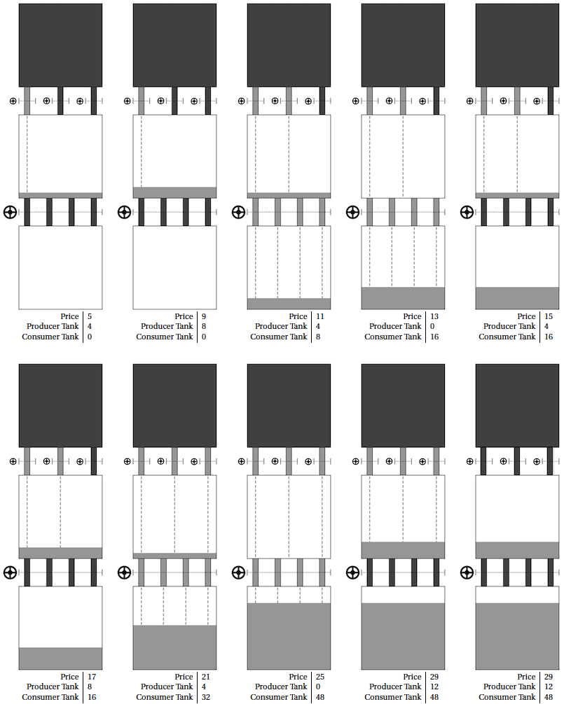
Refer to caption
Figure 2: Valvular auctions and water systems. The top tank is the profit reservoir (drawn as opaque), there are n−1n-1 upper pipes from the profit reservoir to the producer tank, and there are nn lower pipes from the producer tank to the consumer tank. Each upper pipe has its own profit valve and the nn lower pipes are jointly controlled by the regulator’s valve. We illustrate the full process for (i) the example subsidy curve from Figure 1, and (ii) any demand curve where all four agents have valuations above 𝖲​(n)\mathsf{S}(n). For the demand curve in Figure 1, this process simply terminates earlier, at Price 2222, Producer Tank 33, Consumer Tank 3636.

3 Model

3.1 Monopolist environments

We consider a monopolist who can produce identical indivisible objects at a monetary cost. The cost function is weakly convex, and therefore specified by a non-decreasing sequence of marginal costs that (in a slight abuse of terminology131313In standard terminology, supply curves map prices to quantities and inverse supply curves map quantities to prices, but for brevity we use the former term for the latter concept.) we refer to as the supply curve. We allow for both negative marginal costs to allow for objects whose consumption benefits the monopolist and infinite marginal costs to capture infeasible production, and in order to simplify certain edge case arguments, we adopt the convention that the marginal cost at zero is negative infinity.

Definition: The set of (object) quantities is Q≡{0,1,…}Q\equiv\{0,1,...\}. We say that a function 𝖲:Q→ℝ∪{−∞,∞}\mathsf{S}:Q\to\mathbb{R}\cup\{-\infty,\infty\} is a supply curve if (i) 𝖲​(0)=−∞\mathsf{S}(0)=-\infty, (ii) for each q∈{1,2,…}q\in\{1,2,...\} we have 𝖲​(q)∈ℝ∪{∞}\mathsf{S}(q)\in\mathbb{R}\cup\{\infty\}, and (iii) for each q∈Qq\in Q we have 𝖲​(q)≤𝖲​(q+1)\mathsf{S}(q)\leq\mathsf{S}(q+1). For each supply curve 𝖲\mathsf{S}, the associated cost function is the function 𝖢:Q→ℝ∪{∞}\mathsf{C}:Q\to\mathbb{R}\cup\{\infty\} such that for each q∈Qq\in Q, we have

𝖢​(q)≡{∑q′∈⟦1,q⟧𝖲​(q′),𝖲​(q)<∞,∞,𝖲​(q)=∞,\displaystyle\mathsf{C}(q)\equiv\left\{\begin{array}[]{lr}\sum_{q^{\prime}\in\llbracket 1,q\rrbracket}\mathsf{S}(q^{\prime}),&\mathsf{S}(q)<\infty,\\ \infty,&\mathsf{S}(q)=\infty,\end{array}\right.

using the convention that 𝖢​(0)=0\mathsf{C}(0)=0.

The monopolist cannot consume objects, but there are also consumers who can each consume at most one object, and everybody can consume money. We assume the supply curve and the finite set of consumers are common knowledge, while each consumer’s willingness to pay for an object is his private information.

Definition: A (monopolist) environment is a pair (𝖲,N)(\mathsf{S},N) defined as follows.

  • •

    𝖲\mathsf{S} is the supply curve and 𝖢\mathsf{C} is the associated cost function.

  • •

    NN is the finite and nonempty set of consumers. We define n≡|N|n\equiv|N|. There is one producer, the monopolist, denoted by i0∉Ni_{0}\not\in N. Each i∈N∪{i0}i\in N\cup\{i_{0}\} is an agent.

  • •

    For each i∈Ni\in N, the set of (consumption) bundles for ii, denoted XiX_{i}, is a personal copy of ℝ×{0,1}\mathbb{R}\times\{0,1\} for ii,151515Formally, whenever we say that AiA_{i} is a personal copy of space BB for agent ii, we mean that Ai={i}×BA_{i}=\{i\}\times B, so that the space’s owner ii is not only suggested by our usual notation but moreover determined by the space. We then suppress ii in an abuse of notation: for each (i,b)∈{i}×B=Ai(i,b)\in\{i\}\times B=A_{i}, we write b∈Aib\in A_{i}. where each bundle xi=(ti,ai)x_{i}=(t_{i},a_{i}) specifies (monetary) transfer tit_{i} and (object) assignment aia_{i}. We refer to a consumer who receives an object as a winner and a consumer who does not as a loser. As the monopolist cannot consume objects, the set of consumption bundles for i0i_{0}, denoted Xi0X_{i_{0}}, is a personal copy of ℝ×{0}\mathbb{R}\times\{0\} for i0i_{0}.

  • •

    Each i∈Ni\in N has a valuation vi∈ℝv_{i}\in\mathbb{R}, which represents the quasi-linear preference relation ≿i|vi\succsim_{i|v_{i}} over bundles such that for each pair (ti,ai),(ti′,ai′)∈Xi(t_{i},a_{i}),(t_{i}^{\prime},a_{i}^{\prime})\in X_{i},

    (ti,ai)≿i|vi(ti′,ai′)​ if and only if ​vi⋅ai+ti≥vi⋅ai′+ti′.\displaystyle(t_{i},a_{i})\mathrel{\succsim_{i|v_{i}}}(t_{i}^{\prime},a_{i}^{\prime})\text{ if and only if }v_{i}\cdot a_{i}+t_{i}\geq v_{i}\cdot a_{i}^{\prime}+t_{i}^{\prime}.

    This is private information, and the set of possible valuations for ii, denoted ViV_{i}, is a personal copy of ℝ\mathbb{R} for ii. It is common knowledge that the monopolist’s preference relation over Xi0X_{i_{0}}, ≿i0\succsim_{i_{0}}, is the strictly monotonic one. Altogether, the set of possible valuation profiles is V≡×i∈NViV\equiv\times_{i\in N}V_{i}, and to unify notation across consumers and the monopolist, we sometimes write (≿i|v)i∈N∪{i0}(\succsim_{i|v})_{i\in N\cup\{i_{0}\}} for the preference profile determined by vv. As usual, we use ≻\succ instead of ≿\succsim to denote strict preference.

  • •

    We define the production capacity 𝗊cap≡max⁡{q∈⟦0,n⟧|𝖢​(q)<∞}\mathsf{q}^{\text{cap}}\equiv\max\{q\in\llbracket 0,n\rrbracket|\mathsf{C}(q)<\infty\} to be the maximum quantity that can feasibly be produced and consumed. The collection of feasible winner sets is 𝕎≡{W⊆N||W|≤𝗊cap}\mathbb{W}\equiv\{W\subseteq N||W|\leq\mathsf{q}^{\text{cap}}\}, and an outcome is a pair (t,W)∈ℝN×𝕎(t,W)\in\mathbb{R}^{N}\times\mathbb{W}. We let XX denote the set of outcomes, and we associate each (t,W)∈X(t,W)\in X with the allocation in ×i∈N∪{i0}Xi\times_{i\in N\cup\{i_{0}\}}X_{i} such that (i) each consumer ii receives transfer tit_{i}, (ii) WW is the set of winners, and (iii) the monopolist receives the net payment from the consumers and then pays the production costs. Formally, (i) for each i∈Ni\in N, xi​(t,W)≡(ti,|W∩{i}|)x_{i}(t,W)\equiv(t_{i},|W\cap\{i\}|), and (ii) xi0​(t,W)≡([−∑i∈Nti]−𝖢​(|W|),0)x_{i_{0}}(t,W)\equiv([-\sum_{i\in N}t_{i}]-\mathsf{C}(|W|),0).

Whenever we refer to an arbitrary environment, we implicitly assume all of this notation.

3.2 Surplus and efficiency

If the valuation profile were known, then the regulator would be able to evaluate each outcome on the basis of its consumer surplus, producer surplus, and total surplus.

Definition: Fix an environment. For each v∈Vv\in V, each t∈ℝNt\in\mathbb{R}^{N}, and each W∈𝕎W\in\mathbb{W}, we define the associated consumer surplus 𝖢𝖲v​(t,W)\mathsf{CS}_{v}(t,W), producer surplus 𝖯𝖲​(t,W)\mathsf{PS}(t,W), and total surplus 𝖳𝖲v​(W)\mathsf{TS}_{v}(W) by:

𝖢𝖲v​(t,W)\displaystyle\mathsf{CS}_{v}(t,W) ≡∑i∈Wvi+∑i∈Nti,\displaystyle\equiv\sum_{i\in W}v_{i}+\sum_{i\in N}t_{i},
𝖯𝖲​(t,W)\displaystyle\mathsf{PS}(t,W) ≡[−∑i∈Nti]−𝖢​(|W|), and\displaystyle\equiv[-\sum_{i\in N}t_{i}]-\mathsf{C}(|W|),\text{ and}
𝖳𝖲v​(W)\displaystyle\mathsf{TS}_{v}(W) ≡∑i∈Wvi−𝖢​(|W|).\displaystyle\equiv\sum_{i\in W}v_{i}-\mathsf{C}(|W|).

Moreover, for each W∈2N\𝕎W\in 2^{N}\backslash\mathbb{W}, we define 𝖳𝖲v​(W)≡−∞\mathsf{TS}_{v}(W)\equiv-\infty. Observe that because there are no fixed costs, producer surplus is equal to profit: this is precisely the monetary transfer consumed by the monopolist.

Because of our assumption that preferences are quasi-linear, an outcome maximizes total surplus if and only if it is (Pareto) efficient.

Definition: Fix an environment. For each v∈Vv\in V and each (t,W)∈X(t,W)\in X, we say that (t,W)(t,W) is vv-efficient if and only if for each W′∈𝕎W^{\prime}\in\mathbb{W}, 𝖳𝖲v​(W)≥𝖳𝖲v​(W′)\mathsf{TS}_{v}(W)\geq\mathsf{TS}_{v}(W^{\prime}). Equivalently,161616We omit the simple proof; see Chapter 10.E of Mas-Colell, Whinston, and Green (1995). (t,W)(t,W) is vv-efficient if and only if there is no (t′,W′)∈X(t^{\prime},W^{\prime})\in X such that (i) for each i∈N∪{i0}i\in N\cup\{i_{0}\}, xi​(t′,W′)≿i|vxi​(t,W)x_{i}(t^{\prime},W^{\prime})\mathrel{\succsim_{i|v}}x_{i}(t,W), and (ii) for some i∈N∪{i0}i\in N\cup\{i_{0}\}, xi​(t′,W′)≻i|vxi​(t,W)x_{i}(t^{\prime},W^{\prime})\mathrel{\succ_{i|v}}x_{i}(t,W).

3.3 Mechanisms and axioms

The monopolist uses a mechanism to elicit consumer demand and then determine the outcome, and we assume that the regulator is able to constrain which mechanisms are available to the monopolist. As we focus on dominant strategy implementation, we can safely restrict attention to (direct) mechanisms where the consumers simultaneously report their valuations by the classic revelation principle (Gibbard, 1973; Myerson, 1981):

Definition: Fix an environment. A transfer policy is a mapping τ:V→ℝN\tau:V\to\mathbb{R}^{N}, and an assignment policy is a mapping α:V→𝕎\alpha:V\to\mathbb{W}. For each assignment policy α\alpha and each i∈Ni\in N, we let αi\alpha_{i} denote the associated policy for determining whether or not ii is a winner; this is the mapping αi:V→{0,1}\alpha_{i}:V\to\{0,1\} such that for each v∈Vv\in V, αi​(v)=|α​(v)∩{i}|\alpha_{i}(v)=|\alpha(v)\cap\{i\}|. A mechanism (τ,α)(\tau,\alpha) consists of a transfer policy τ\tau and an assignment policy α\alpha.

The regulator may require the mechanism to satisfy certain properties that we refer to as axioms, and our analysis involves the following ones.

Definition: Fix an environment. A mechanism (τ,α)(\tau,\alpha) satisfies

  • •

    efficiency if for each v∈Vv\in V, (τ​(v),α​(v))(\tau(v),\alpha(v)) is vv-efficient;

  • •

    strategy-proofness if for each i∈Ni\in N, each v−i∈V−iv_{-i}\in V_{-i}, and each pair vi,vi′∈Viv_{i},v_{i}^{\prime}\in V_{i}, we have vi⋅αi​(v)+τi​(v)≥vi⋅αi​(vi′,v−i)+τi​(vi′,v−i)v_{i}\cdot\alpha_{i}(v)+\tau_{i}(v)\geq v_{i}\cdot\alpha_{i}(v_{i}^{\prime},v_{-i})+\tau_{i}(v_{i}^{\prime},v_{-i});

  • •

    no-envy if for each v∈Vv\in V and each pair i,j∈Ni,j\in N, vi⋅αi​(v)+τi​(v)≥vi⋅αj​(v)+τj​(v)v_{i}\cdot\alpha_{i}(v)+\tau_{i}(v)\geq v_{i}\cdot\alpha_{j}(v)+\tau_{j}(v);

  • •

    consumer voluntary participation if for each v∈Vv\in V and each i∈Ni\in N, we have vi⋅αi​(v)+τi​(v)≥0v_{i}\cdot\alpha_{i}(v)+\tau_{i}(v)\geq 0;

  • •

    producer voluntary participation if for each v∈Vv\in V, [−∑i∈Nτi​(v)]−𝖢​(|α​(v)|)≥0[-\sum_{i\in N}\tau_{i}(v)]-\mathsf{C}(|\alpha(v)|)\geq 0; and

  • •

    voluntary participation if it satisfies both consumer voluntary participation and producer voluntary participation.

We say that an assignment policy α\alpha is surplus-maximizing if and only if for each v∈Vv\in V and each W∈𝕎W\in\mathbb{W}, 𝖳𝖲v​(α​(v))≥𝖳𝖲v​(W)\mathsf{TS}_{v}(\alpha(v))\geq\mathsf{TS}_{v}(W). Equivalently, α\alpha is surplus-maximizing if and only if for each transfer policy τ\tau, the mechanism (τ,α)(\tau,\alpha) satisfies efficiency.

The first three axioms represent constraints imposed by the regulator that we fix throughout our analysis. The first implies that the monopolist cannot reduce production from the efficient level in order to increase the price, the second requires that it is always a dominant strategy for each customer to honestly reveal his valuation, and the third captures the idea that the auction should output equal opportunities. The remaining axioms are ex-post voluntary participation constraints that prevent arbitrary transfers from one side of the market to the other; these are also known as individual rationality constraints in the literature.

4 Preliminary lemmas

We study a particularly simple auction model: there is unit demand, objects are identical, and preferences are quasi-linear. As a result, many known results apply to our model as a special case, and our main results involve many familiar ideas. The purpose of this section is to gather the familiar ideas that are necessary for stating our main results and discussing the underlying intuition. For the proofs of all lemmas in this section, see Appendix A.

4.1 Complete information

When we pair an environment with a valuation profile, we have a complete information economy that is ripe for classic supply-demand analysis. We begin by introducing the reported demand curve and using it to provide explicit formulas for the endpoints of the interval of efficient quantities. Moreover, in anticipation of their later usefulness, we also introduce these ideas for economies with a single consumer removed.

Definition: Fix an environment. For each v∈Vv\in V, we define (i) the demand curve given vv, 𝖣v:Q→ℝ∪{−∞,∞}\mathsf{D}_{v}:Q\to\mathbb{R}\cup\{-\infty,\infty\}, (ii) the minimum efficient quantity given vv, 𝗊vmin∈Q\mathsf{q}^{\min}_{v}\in Q, and (iii) the maximum efficient quantity given vv, 𝗊vmax∈Q\mathsf{q}^{\max}_{v}\in Q, as follows.

  • •

    𝖣v​(0)≡∞\mathsf{D}_{v}(0)\equiv\infty, (𝖣v​(q))q∈⟦1,n⟧(\mathsf{D}_{v}(q))_{q\in\llbracket 1,n\rrbracket} re-orders (vj)j∈N(v_{j})_{j\in N} such that 𝖣v​(1)≥𝖣v​(2)≥…≥𝖣v​(n)\mathsf{D}_{v}(1)\geq\mathsf{D}_{v}(2)\geq...\geq\mathsf{D}_{v}(n), and q>nq>n implies 𝖣v​(q)≡−∞\mathsf{D}_{v}(q)\equiv-\infty;

  • •

    𝗊vmin≡max⁡{q∈Q​|𝖣v​(q)>​𝖲​(q)}\mathsf{q}^{\min}_{v}\equiv\max\{q\in Q|\mathsf{D}_{v}(q)>\mathsf{S}(q)\} and 𝗊vmax≡max⁡{q∈Q|𝖣v​(q)≥𝖲​(q)}\mathsf{q}^{\max}_{v}\equiv\max\{q\in Q|\mathsf{D}_{v}(q)\geq\mathsf{S}(q)\}.

Similarly, for each i∈Ni\in N and each v−i∈V−iv_{-i}\in V_{-i}, we define 𝖣v−i:Q→ℝ∪{−∞,∞}\mathsf{D}_{v_{-i}}:Q\to\mathbb{R}\cup\{-\infty,\infty\}, 𝗊v−imin∈Q\mathsf{q}^{\min}_{v_{-i}}\in Q, and 𝗊v−imax∈Q\mathsf{q}^{\max}_{v_{-i}}\in Q as follows.

  • •

    𝖣v−i​(0)≡∞\mathsf{D}_{v_{-i}}(0)\equiv\infty, (𝖣v−i​(q))q∈⟦1,n−1⟧(\mathsf{D}_{v_{-i}}(q))_{q\in\llbracket 1,n-1\rrbracket} re-orders (vj)j∈N\{i}(v_{j})_{j\in N\backslash\{i\}} such that 𝖣v−i​(1)≥𝖣v−i​(2)≥…≥𝖣v−i​(n−1)\mathsf{D}_{v_{-i}}(1)\geq\mathsf{D}_{v_{-i}}(2)\geq...\geq\mathsf{D}_{v_{-i}}(n-1), and q>n−1q>n-1 implies 𝖣v−i​(q)≡−∞\mathsf{D}_{v_{-i}}(q)\equiv-\infty;

  • •

    𝗊v−imin≡max⁡{q∈Q​|𝖣v−i​(q)>​𝖲​(q)}\mathsf{q}^{\min}_{v_{-i}}\equiv\max\{q\in Q|\mathsf{D}_{v_{-i}}(q)>\mathsf{S}(q)\} and 𝗊v−imax≡max⁡{q∈Q|𝖣v−i​(q)≥𝖲​(q)}\mathsf{q}^{\max}_{v_{-i}}\equiv\max\{q\in Q|\mathsf{D}_{v_{-i}}(q)\geq\mathsf{S}(q)\}.

Our terminology for these quantities is justified by the following lemma.

Quantity Lemma: Fix an environment and let v∈Vv\in V. For each (t,W)∈X(t,W)\in X, (t,W)(t,W) is vv-efficient if and only if (i) |W|∈⟦𝗊vmin,𝗊vmax⟧|W|\in\llbracket\mathsf{q}^{\min}_{v},\mathsf{q}^{\max}_{v}\rrbracket, and (ii) there is no loser with a higher valuation than a winner: for each i∈Wi\in W and each j∈N\Wj\in N\backslash W, we have vi≥vjv_{i}\geq v_{j}.

Similarly, we can use the reported demand curve and the known supply curve to determine an interval on the price axis. In particular, recall that in the sense of the second welfare theorem, a competitive equilibrium is an efficient outcome supported by some redistribution and market prices. In general, redistribution might involve a combination of commodities and ownership shares, but in partial equilibrium models such as this one, redistribution of the numeraire suffices to support all efficient outcomes; see Chapter 10.D of Mas-Colell, Whinston, and Green (1995). We therefore consider competitive equilibria that are supported by (i) a profile of subsidies, or monetary transfers, with a negative subsidy understood as a tax, and (ii) a single market price for objects. To define them, we first introduce the relevant budget sets and demand sets for consumers.

Definition: Fix an environment. For each i∈Ni\in N, each subsidy si∈ℝs_{i}\in\mathbb{R}, each price p∈ℝ∪{∞}p\in\mathbb{R}\cup\{\infty\}, and each valuation vi∈Viv_{i}\in V_{i}, the associated budget set boundary Bi​(si,p)⊆XiB_{i}(s_{i},p)\subseteq X_{i} and demand set Biδ​(si,p|vi)⊆Bi​(si,p)B^{\delta}_{i}(s_{i},p|v_{i})\subseteq B_{i}(s_{i},p) are

Bi​(si,p)\displaystyle B_{i}(s_{i},p) ≡{{(si,0),(si−p,1)},p∈ℝ,{(si,0)},p=∞; and\displaystyle\equiv\left\{\begin{array}[]{lr}\{(s_{i},0),(s_{i}-p,1)\},&p\in\mathbb{R},\\ \{(s_{i},0)\},&p=\infty;\text{ and}\end{array}\right.
Biδ​(si,p|vi)\displaystyle B^{\delta}_{i}(s_{i},p|v_{i}) ≡arg​max(ti,ai)∈Bi​(si,p)⁡[vi⋅ai+ti].\displaystyle\equiv\operatorname*{arg\,max}_{(t_{i},a_{i})\in B_{i}(s_{i},p)}[v_{i}\cdot a_{i}+t_{i}].

In our setting, a simple interpretation of competitive equilibrium is that only the numeraire is redistributed and then “the market works,” with the monopolist behaving as a price taker. That said, certain subsidy profiles allow for the interpretation that only ownership shares are redistributed, from the monopolist to the consumers, with all consumers receiving the same shareholding.

Definition: Fix an environment, let v∈Vv\in V, let (t∗,W∗)∈X(t^{*},W^{*})\in X, let (ai∗)i∈N∈{0,1}N(a^{*}_{i})_{i\in N}\in\{0,1\}^{N} denote the associated assignment profile, and define q∗≡|W∗|q^{*}\equiv|W^{*}|. For each subsidy profile s∈ℝNs\in\mathbb{R}^{N} and each price p∈ℝ∪{∞}p\in\mathbb{R}\cup\{\infty\}, we say that (t∗,W∗)(t^{*},W^{*}) is a competitive equilibrium supported by (s,p)(s,p) if and only if

  • •

    for each i∈Ni\in N, we have (ti∗,ai∗)∈Biδ​(si,p|vi)(t^{*}_{i},a^{*}_{i})\in B^{\delta}_{i}(s_{i},p|v_{i}), and

  • •

    the monopolist selects q∗q^{*} to maximize profit in response to pp, or equivalently,

    (i) p∈ℝp\in\mathbb{R} implies q∗∈arg​maxq∈{q′∈Q|𝖢​(q′)<∞}⁡[p⋅q−𝖢​(q)]q^{*}\in\operatorname*{arg\,max}_{q\in\{q^{\prime}\in Q|\mathsf{C}(q^{\prime})<\infty\}}[p\cdot q-\mathsf{C}(q)], and

    (ii) p=∞p=\infty implies q∗=max⁡{q′∈Q|𝖢​(q′)<∞}q^{*}=\max\{q^{\prime}\in Q|\mathsf{C}(q^{\prime})<\infty\}.

If moreover there is a consumer subsidy sN∈ℝs_{N}\in\mathbb{R} such that for each i∈Ni\in N we have si=sNs_{i}=s_{N}, then we say that (t∗,W∗)(t^{*},W^{*}) is an equal subsidy equilibrium supported by (sN,p)(s_{N},p). Finally, if moreover there is a consumer shareholding \textfraks:N∈[0,1n]\textfrak{s:}_{N}\in[0,\frac{1}{n}] such that either (i) |W∗|=0|W^{*}|=0 and sN=0s_{N}=0, or (ii) |W∗|>0|W^{*}|>0 and sN=\textfraks:N⋅(p⋅|W∗|−𝖢(|W∗|))s_{N}=\textfrak{s:}_{N}\cdot(p\cdot|W^{*}|-\mathsf{C}(|W^{*}|)), so that the consumer subsidy is the associated dividend of the profit, then we say that (t∗,W∗)(t^{*},W^{*}) is an equal shareholding equilibrium supported by (\textfraks:N,p)(\textfrak{s:}_{N},p). We emphasize that if an equal shareholding equilibrium has zero profit, which includes the case of an infinite price with no production, then the equilibrium can be supported by any consumer shareholding.

We can establish the existence of competitive equilibria in our setting by appealing to known results about the assignment game, in which unit demand buyers match with unit supply sellers and money can be transferred. Indeed, we can analyze each environment and valuation profile using an associated assignment game with nn buyers and 𝗊cap\mathsf{q}^{\text{cap}} sellers whose valuations are respectively summarized by 𝖣v\mathsf{D}_{v} and 𝖲\mathsf{S}, as the competitive equilibria for the two economies coincide. In the assignment game, the set of competitive prices is nonempty (Koopmans and Beckmann, 1957) and moreover a lattice (Shapley and Shubik, 1972), and because we consider the special case where the objects are identical (Böhm-Bawerk, 1888), this lattice is simply an interval.

As with the interval of efficient quantities, we can provide explicit formulas for the endpoints of the interval of competitive prices. In general, a competitive price may lie outside the interval of relevant marginal costs, but these extreme prices are never necessary: (i) p<𝖲​(1)p<\mathsf{S}(1) implies no production, which can also be supported with p′=𝖲​(1)p^{\prime}=\mathsf{S}(1), and (ii) p>𝖲​(n)p>\mathsf{S}(n) implies full production, which can also be supported with p′=𝖲​(n)p^{\prime}=\mathsf{S}(n). We therefore also introduce rounded competitive prices for situations where it is useful to avoid these unnecessary extreme prices.

Definition: Fix an environment. For each v∈Vv\in V, we define (i) the minimum competitive price given vv, 𝗉vmin∈ℝ\mathsf{p}^{\min}_{v}\in\mathbb{R}, (ii) the maximum competitive price given vv, 𝗉vmax∈ℝ∪{∞}\mathsf{p}^{\max}_{v}\in\mathbb{R}\cup\{\infty\}, (iii) the rounded minimum competitive price given vv, 𝗉vmin↑∈ℝ∪{∞}\mathsf{p}^{\min\uparrow}_{v}\in\mathbb{R}\cup\{\infty\}, and (iv) the rounded maximum competitive price given vv, 𝗉vmax↓∈ℝ∪{∞}\mathsf{p}^{\max\downarrow}_{v}\in\mathbb{R}\cup\{\infty\}, as follows.

  • •

    𝗉vmin≡max⁡{𝖣v​(𝗊vmax+1),𝖲​(𝗊vmax)}\mathsf{p}^{\min}_{v}\equiv\max\{\mathsf{D}_{v}(\mathsf{q}^{\max}_{v}+1),\mathsf{S}(\mathsf{q}^{\max}_{v})\} and 𝗉vmax≡min⁡{𝖣v​(𝗊vmax),𝖲​(𝗊vmax+1)}\mathsf{p}^{\max}_{v}\equiv\min\{\mathsf{D}_{v}(\mathsf{q}^{\max}_{v}),\mathsf{S}(\mathsf{q}^{\max}_{v}+1)\}; and

  • •

    𝗉vmin↑≡max⁡{𝗉vmin,𝖲​(1)}\mathsf{p}^{\min\uparrow}_{v}\equiv\max\{\mathsf{p}^{\min}_{v},\mathsf{S}(1)\} and 𝗉vmax↓≡min⁡{𝗉vmax,𝖲​(n)}\mathsf{p}^{\max\downarrow}_{v}\equiv\min\{\mathsf{p}^{\max}_{v},\mathsf{S}(n)\}.

Our terminology for these competitive prices will be justified by our next lemma, which also relates them to the following individualized prices.

Definition: Fix an environment. For each i∈Ni\in N and each v−i∈V−iv_{-i}\in V_{-i}, we define the Groves price given v−iv_{-i}, 𝗉v−iγ∈ℝ∪{∞}\mathsf{p}^{\gamma}_{v_{-i}}\in\mathbb{R}\cup\{\infty\}, by

𝗉v−iγ≡min⁡{𝖣v−i​(𝗊v−imax),𝖲​(𝗊v−imax+1)}.\displaystyle\mathsf{p}^{\gamma}_{v_{-i}}\equiv\min\{\mathsf{D}_{v_{-i}}(\mathsf{q}^{\max}_{v_{-i}}),\mathsf{S}(\mathsf{q}^{\max}_{v_{-i}}+1)\}.

When the Groves price 𝗉v−iγ\mathsf{p}^{\gamma}_{v_{-i}} is finite, it has the property that vi−𝗉v−iγv_{i}-\mathsf{p}^{\gamma}_{v_{-i}} is the marginal contribution of ii to total surplus: it is the difference between the optimal total surplus of a group that includes ii and the optimal total surplus of a group that excludes ii. Intuitively, it has this particular structure in our model because we can always optimally exclude ii by selecting the 𝗊v−imax\mathsf{q}^{\max}_{v_{-i}} highest-valuation peers of ii, but sometimes it is optimal for ii to replace one of these peers and other times it is optimal for ii to join them. In the general context of Groves mechanisms, which are characterized by efficiency and strategy-proofness (Holmström, 1979), 𝗉v−iγ\mathsf{p}^{\gamma}_{v_{-i}} is sometimes described as the externality that ii imposes on his peers, or the VCG payment, and our terminology reflects its central role in the full class of Groves mechanisms. That said, we emphasize that our next lemma involves only efficiency.

In the specific context of auctions with unit demand and quasi-linear preferences, it is well-known that a VCG mechanism is a minimum competitive price mechanism (Demange, 1982; Leonard, 1983), in which winners pay and the losers refuse the minimum competitive prices. For example, in an auction for one object, the winner pays the second-highest valuation, the losers refuse the second-highest valuation, and a price is competitive if and only if it is between the second-highest valuation and the highest valuation. Rarely emphasized, but important to our analysis, is the observation that the losers also refuse the maximum competitive prices. For example, in an auction for one object, each loser refuses the highest valuation. In the following lemma, we gather this observation and other useful relationships between competitive prices, rounded competitive prices, and Groves prices.

Price Lemma: Fix an environment and let v∈Vv\in V. First, for each p∈ℝ∪{∞}p\in\mathbb{R}\cup\{\infty\}, there are a subsidy profile s∈ℝNs\in\mathbb{R}^{N} and a competitive equilibrium supported by (s,p)(s,p) if and only if p∈[𝗉vmin,𝗉vmax]p\in[\mathsf{p}^{\min}_{v},\mathsf{p}^{\max}_{v}]. Second, for each i∈Ni\in N, we have either

  • •

    vi≥𝖣v​(𝗊vmax)≥𝗉vmax≥𝗉vmax↓≥𝗉vmin↑=𝗉vmin=𝗉v−iγ≥𝖣v​(𝗊vmax+1)v_{i}\geq\mathsf{D}_{v}(\mathsf{q}^{\max}_{v})\geq\mathsf{p}^{\max}_{v}\geq\mathsf{p}^{\max\downarrow}_{v}\geq\mathsf{p}^{\min\uparrow}_{v}=\mathsf{p}^{\min}_{v}=\mathsf{p}^{\gamma}_{v_{-i}}\geq\mathsf{D}_{v}(\mathsf{q}^{\max}_{v}+1), or

  • •

    𝖣v​(𝗊vmax)≥𝗉v−iγ=𝗉vmax=𝗉vmax↓≥𝗉vmin↑≥𝗉vmin≥𝖣v​(𝗊vmax+1)≥vi\mathsf{D}_{v}(\mathsf{q}^{\max}_{v})\geq\mathsf{p}^{\gamma}_{v_{-i}}=\mathsf{p}^{\max}_{v}=\mathsf{p}^{\max\downarrow}_{v}\geq\mathsf{p}^{\min\uparrow}_{v}\geq\mathsf{p}^{\min}_{v}\geq\mathsf{D}_{v}(\mathsf{q}^{\max}_{v}+1)\geq v_{i}.

Third, for each (t,W)∈X(t,W)\in X that is vv-efficient and each i∈Ni\in N, vi>𝗉v−iγv_{i}>\mathsf{p}^{\gamma}_{v_{-i}} implies i∈Wi\in W and 𝗉v−iγ>vi\mathsf{p}^{\gamma}_{v_{-i}}>v_{i} implies i∉Wi\not\in W. Finally, if 𝖲​(1)≠∞\mathsf{S}(1)\neq\infty, then for each i∈Ni\in N,

𝗉v−iγ=vi−[maxW∈𝕎,i∈W⁡𝖳𝖲v​(W)−maxW′∈𝕎,i∉W′⁡𝖳𝖲v​(W′)].\displaystyle\mathsf{p}^{\gamma}_{v_{-i}}=v_{i}-[\max_{W\in\mathbb{W},i\in W}\mathsf{TS}_{v}(W)-\max_{W^{\prime}\in\mathbb{W},i\not\in W^{\prime}}\mathsf{TS}_{v}(W^{\prime})].

Our Price Lemma reinforces insights from a link between extreme competitive prices and VCG payments in the context of two-sided environments with single-object traders (Delacrétaz, Loertscher, and Mezzetti, 2022): “[ …]the–extremal–Walrasian prices provide the traders with precisely the right incentives to reveal their valuations. The subtle but important twist is that incentive compatible information revelation requires the use of two different Walrasian prices for every object that is traded [ …]”

Finally, it will prove useful to distinguish the interval of Groves prices from the interval of competitive prices, to divide the former into subintervals using the marginal costs, and to observe that whenever a possible Groves price is the common valuation of all consumers, it is also the common Groves price of all consumers.

Definition: Fix an environment. We define the Groves price interval, ℙ⊆ℝ∪{∞}\mathbb{P}\subseteq\mathbb{R}\cup\{\infty\}, by

ℙ\displaystyle\mathbb{P} ={[𝖲​(1),𝖲​(n)]\{∞},𝖲​(1)≠∞,{∞},𝖲​(1)=∞.\displaystyle=\left\{\begin{array}[]{lr}[\mathsf{S}(1),\mathsf{S}(n)]\backslash\{\infty\},&\mathsf{S}(1)\neq\infty,\\ \{\infty\},&\mathsf{S}(1)=\infty.\end{array}\right.

We define the set of Groves price subintervals, {ℙq}q∈⟦1,𝗊cap⟧\{\mathbb{P}_{q}\}_{q\in\llbracket 1,\mathsf{q}^{\text{cap}}\rrbracket}, as follows: (i) for each q∈⟦1,𝗊cap−1⟧q\in\llbracket 1,\mathsf{q}^{\text{cap}}-1\rrbracket, ℙq≡[𝖲​(q),𝖲​(q+1)]\mathbb{P}_{q}\equiv[\mathsf{S}(q),\mathsf{S}(q+1)], (ii) if 𝗊cap=n\mathsf{q}^{\text{cap}}=n, then ℙ𝗊cap={𝖲​(𝗊cap)}\mathbb{P}_{\mathsf{q}^{\text{cap}}}=\{\mathsf{S}(\mathsf{q}^{\text{cap}})\}, and (ii) if 𝗊cap<n\mathsf{q}^{\text{cap}}<n, then ℙ𝗊cap≡[𝖲​(𝗊cap),∞)\mathbb{P}_{\mathsf{q}^{\text{cap}}}\equiv[\mathsf{S}(\mathsf{q}^{\text{cap}}),\infty). Observe that if 𝖲​(1)=∞\mathsf{S}(1)=\infty, then there are no Groves price subintervals.

Interval Lemma: Fix an environment. First, for each p∈ℙp\in\mathbb{P}, if v∈Vv\in V is such that each consumer has valuation pp, then for each i∈Ni\in N we have 𝗉v−iγ=p\mathsf{p}^{\gamma}_{v_{-i}}=p. Second, for each i∈Ni\in N, ℙ={𝗉v−iγ|v−i∈V−i}\mathbb{P}=\{\mathsf{p}^{\gamma}_{v_{-i}}|v_{-i}\in V_{-i}\}. Finally, 𝖲​(1)≠∞\mathsf{S}(1)\neq\infty implies ℙ=∪q∈⟦1,𝗊cap⟧ℙq\mathbb{P}=\cup_{q\in\llbracket 1,\mathsf{q}^{\text{cap}}\rrbracket}\mathbb{P}_{q}.

4.2 Incomplete information

We now turn to our preliminary lemmas about mechanisms, and begin by observing that efficiency, strategy-proofness, and no-envy are all closely related to budget sets. First, by the second welfare theorem, efficiency is equivalent to the requirement that at each valuation profile, the consumers select from personalized budget sets that share a market price, and moreover the monopolist selects a quantity to maximize profit given this market price. Second, strategy-proofness is equivalent to the requirement that at each valuation profile, each consumer selects from a personalized budget set determined by his peers. Finally, no-envy is equivalent to the requirement that at each valuation profile, the consumers select from a common consumer budget set.

Budget Set Lemma: Fix an environment. A mechanism (τ,α)(\tau,\alpha) satisfies

  • (i)

    efficiency if and only if for each v∈Vv\in V, there is personalized subsidy profile (si​(v))i∈N∈ℝN(s_{i}(v))_{i\in N}\in\mathbb{R}^{N} and market price pN0​(v)∈[𝗉vmin,𝗉vmax]p_{N_{0}}(v)\in[\mathsf{p}^{\min}_{v},\mathsf{p}^{\max}_{v}] such that (τ​(v),α​(v))(\tau(v),\alpha(v)) is a competitive equilibrium supported by ((si​(v))i∈N,pN0​(v))((s_{i}(v))_{i\in N},p_{N_{0}}(v));

  • (ii)

    strategy-proofness if and only if for each i∈Ni\in N and each v−i∈V−iv_{-i}\in V_{-i}, either

    • ∙\bullet

      there is personalized bundle xi​(v−i)∈Xix_{i}(v_{-i})\in X_{i} such that for each vi∈Viv_{i}\in V_{i}, we have (τi​(v),αi​(v))=xi​(v−i)(\tau_{i}(v),\alpha_{i}(v))=x_{i}(v_{-i}), or

    • ∙\bullet

      there are personalized subsidy si​(v−i)∈ℝs_{i}(v_{-i})\in\mathbb{R} and personalized price pi​(v−i)∈ℝp_{i}(v_{-i})\in\mathbb{R} such that for each vi∈Viv_{i}\in V_{i}, we have (τi​(v),αi​(v))∈Biδ​(si​(v−i),pi​(v−i)|vi)(\tau_{i}(v),\alpha_{i}(v))\in B^{\delta}_{i}(s_{i}(v_{-i}),p_{i}(v_{-i})|v_{i}); and

  • (iii)

    no-envy if and only if for each v∈Vv\in V, there are consumer subsidy sN​(v)∈ℝs_{N}(v)\in\mathbb{R} and consumer price pN​(v)∈ℝp_{N}(v)\in\mathbb{R} such that for each i∈Ni\in N, we have (τi​(v),αi​(v))∈Biδ​(sN​(v),pN​(v)|vi)(\tau_{i}(v),\alpha_{i}(v))\in B^{\delta}_{i}(s_{N}(v),p_{N}(v)|v_{i}).

Though it is not obvious from inspection that any mechanism simultaneously satisfies all three requirements, it is well-known that in fact the VCG mechanisms do, and that they moreover satisfy voluntary participation. Our primary contribution is to show that they are not alone.

The VCG mechanisms are certainly not alone if we drop no-envy: by a superficial modification of Holmström (1979) to allow for cost functions, the class of mechanisms satisfying efficiency and strategy-proofness is precisely the class of Groves mechanisms. In the usual definition, each consumer’s transfer is the sum of (i) the reported peer surplus at the selected decision, and (ii) a bonus determined entirely by his peers. For our purposes, it is useful to work with an equivalent definition: each consumer selects his favorite bundle from his option set, or collection of attainable bundles given his peers’ reports, and this is a budget set whose subsidy is determined entirely by his peers and whose price is the Groves price.

Definition: Fix an environment. A mechanism (τ,α)(\tau,\alpha) is a Groves mechanism if and only if (i) α\alpha is surplus-maximizing, and (ii) for each i∈Ni\in N, there is (peer) bonus function βi:V−i→ℝ\beta_{i}:V_{-i}\to\mathbb{R} such that for each v∈Vv\in V, we have

τi​(v)=([maxW⊆N⁡𝖳𝖲v​(W)]−αi​(v)​vi)+βi​(v−i).\displaystyle\tau_{i}(v)=\big([\max_{W\subseteq N}\mathsf{TS}_{v}(W)]-\alpha_{i}(v)v_{i}\big)+\beta_{i}(v_{-i}).

Groves Lemma: Fix an environment and let (τ,α)(\tau,\alpha) be an efficient mechanism. The following are equivalent:

  • (i)

    (τ,α)(\tau,\alpha) is strategy-proof;

  • (ii)

    (τ,α)(\tau,\alpha) is a Groves mechanism; and

  • (iii)

    for each i∈Ni\in N, there is a subsidy function σi:V−i→ℝ\sigma_{i}:V_{-i}\to\mathbb{R} such that for each v∈Vv\in V, we have (τi​(v),αi​(v))∈Biδ​(σi​(v−i),𝗉v−iγ|vi)(\tau_{i}(v),\alpha_{i}(v))\in B^{\delta}_{i}(\sigma_{i}(v_{-i}),\mathsf{p}^{\gamma}_{v_{-i}}|v_{i}).

We define the VCG mechanisms as Groves mechanisms for which each consumer’s transfer is precisely the difference between (i) the reported peer surplus at the selected decision, and (ii) the optimal reported peer surplus provided that ii must be excluded. This exclusion provision is a twist on the usual definition that protects a loser from paying when there are negative costs, but has no bite in the usual scenario where costs are non-negative; see the comparison of standard pivot mechanisms and exclusion pivot mechanisms in Mackenzie and Trudeau (2023). Again, there is a useful equivalent definition involving option sets: the VCG mechanisms are the Groves mechanisms for which each option set is a budget whose subsidy is zero and whose price is the Groves price. Finally, there is a third equivalent definition: a VCG mechanism is a minimum competitive price mechanism (Demange, 1982; Leonard, 1983).

Definition: Fix an environment. A Groves mechanism (τ,α)(\tau,\alpha) is moreover a VCG mechanism if and only if for each i∈Ni\in N and each v∈Vv\in V, we have

τi​(v)=([maxW⊆N⁡𝖳𝖲v​(W)]−αi​(v)​vi)−[maxW⊆N\{i}⁡𝖳𝖲(0,v−i)​(W)].\displaystyle\tau_{i}(v)=\big([\max_{W\subseteq N}\mathsf{TS}_{v}(W)]-\alpha_{i}(v)v_{i}\big)-[\max_{W\subseteq N\backslash\{i\}}\mathsf{TS}_{(0,v_{-i})}(W)].

VCG Lemma: Fix an environment and let (τ,α)(\tau,\alpha) be a Groves mechanism. The following are equivalent:

  • (i)

    (τ,α)(\tau,\alpha) is a VCG mechanism;

  • (ii)

    for each i∈Ni\in N and each v∈Vv\in V, (τi​(v),αi​(v))∈Biδ​(0,𝗉v−iγ|vi)(\tau_{i}(v),\alpha_{i}(v))\in B^{\delta}_{i}(0,\mathsf{p}^{\gamma}_{v_{-i}}|v_{i}); and

  • (iii)

    for each i∈Ni\in N and each v∈Vv\in V, (τi​(v),αi​(v))∈Biδ​(0,𝗉vmin|vi)(\tau_{i}(v),\alpha_{i}(v))\in B^{\delta}_{i}(0,\mathsf{p}^{\min}_{v}|v_{i}).

5 Main results

Before we proceed, we remark that the proofs of results in Section 5.1, Section 5.2, Section 5.3, and Section 5.4 can be found, respectively, in Appendix B, Appendix C, Appendix D, and Appendix E.

5.1 Endogenous subsidy auctions

It is easy to see that the VCG mechanisms are not the only envy-free Groves mechanisms. Indeed, we can modify any VCG mechanism by always transferring an exogenous subsidy to each consumer from the monopolist, and the quasilinearity of preferences ensures that all axioms are preserved. This is not particularly appealing, however, because the only exogenous subsidy that guarantees ex-post voluntary participation for all parties is zero.

A more appealing direction would be to design subsidies that preserve all axioms and yet vary with the auction’s outcome, and the simplest approach would be to assign an exogenous share of the auction’s profit to each consumer. Unfortunately, however, this simple approach does not preserve strategy-proofness. For example, in an auction for one object, if we modify the Vickrey auction by assigning a positive share of the profit to each consumer, then the profit is the second highest bid; thus for any consumer who is convinced that the highest bid will be above his own valuation, there is an incentive to misreport.

That said, it turns out that it is possible to design an endogenous subsidy that preserves all axioms. The construction is rather delicate: the subsidy to each consumer must be determined by his peers, it must moreover vary only with the Groves price, and it must moreover vary continuously with the Groves price in a particular way. All of this structure is driven by our key lemma.

Invariance Lemma: Fix an environment. If a mechanism (τ,α)(\tau,\alpha) satisfies efficiency, strategy-proofness, and no-envy, then for each i∈Ni\in N, there is a subsidy function σi:V−i→ℝ\sigma_{i}:V_{-i}\to\mathbb{R} such that

(i) for each v∈Vv\in V, (τi​(v),αi​(v))∈Biδ​(σi​(v−i),𝗉v−iγ|vi)(\tau_{i}(v),\alpha_{i}(v))\in B^{\delta}_{i}(\sigma_{i}(v_{-i}),\mathsf{p}^{\gamma}_{v_{-i}}|v_{i}), and

(ii) for each pair v−i,v−i′∈V−iv_{-i},v_{-i}^{\prime}\in V_{-i}, 𝗉v−iγ=𝗉v−i′γ\mathsf{p}^{\gamma}_{v_{-i}}=\mathsf{p}^{\gamma}_{v_{-i}^{\prime}} implies σi​(v−i)=σi​(v−i′)\sigma_{i}(v_{-i})=\sigma_{i}(v_{-i}^{\prime}).

For this particular proof, we provide a proof sketch in Section 6. As a result of our key lemma, under these three axioms, the subsidy function of a consumer ii, σi:V−i→ℝ\sigma_{i}:V_{-i}\to\mathbb{R}, is determined entirely by an associated function that maps Groves prices to subsidies. In fact, there is one such function shared by all consumers, and it has some structure.

Definition: Fix an environment. A subsidy curve is a function ς:ℙ→ℝ\varsigma:\mathbb{P}\to\mathbb{R} such that for each pair p,p′∈ℙp,p^{\prime}\in\mathbb{P} such that p′>pp^{\prime}>p, we have ς​(p′)−ς​(p)p′−p∈[0,1]\frac{\varsigma(p^{\prime})-\varsigma(p)}{p^{\prime}-p}\in[0,1]. The associated extended subsidy curve, ς↔\varsigma^{\leftrightarrow}, is defined in two cases.

  • •

    If 𝖲​(1)≠∞\mathsf{S}(1)\neq\infty, then ς↔:ℝ→ℝ\varsigma^{\leftrightarrow}:\mathbb{R}\to\mathbb{R} is the function such that for each p∈ℝp\in\mathbb{R}, (i) p<𝖲​(1)p<\mathsf{S}(1) implies ς↔​(p)=ς​(𝖲​(1))\varsigma^{\leftrightarrow}(p)=\varsigma(\mathsf{S}(1)), (ii) p>𝖲​(n)p>\mathsf{S}(n) implies ς↔​(p)=ς​(𝖲​(n))\varsigma^{\leftrightarrow}(p)=\varsigma(\mathsf{S}(n)), and (iii) otherwise ς↔​(p)=ς​(p)\varsigma^{\leftrightarrow}(p)=\varsigma(p). In this case, ς↔\varsigma^{\leftrightarrow} extends ς\varsigma from ℙ⊆ℝ\mathbb{P}\subseteq\mathbb{R} to ℝ\mathbb{R}.

  • •

    If 𝖲​(1)=∞\mathsf{S}(1)=\infty, then ς↔:ℝ∪{∞}→ℝ\varsigma^{\leftrightarrow}:\mathbb{R}\cup\{\infty\}\to\mathbb{R} is the function such that for each p∈ℝ∪{∞}p\in\mathbb{R}\cup\{\infty\}, ς↔​(p)=ς​(∞)\varsigma^{\leftrightarrow}(p)=\varsigma(\infty). In this case, ς↔\varsigma^{\leftrightarrow} extends ς\varsigma from ℙ={∞}\mathbb{P}=\{\infty\} to ℝ∪{∞}\mathbb{R}\cup\{\infty\}.

In an endogenous subsidy auction, a single subsidy curve is used to determine the subsidies for all consumers. More precisely, for each surplus-maximizing assignment policy α\alpha and each subsidy curve ς\varsigma, the associated endogenous subsidy auction can be described as follows: (i) take the outcome of the VCG mechanism associated with α\alpha, and then (ii) transfer to each consumer the subsidy that ς\varsigma assigns to his personal Groves price. In the special case that the subsidy curve is flat at zero, this is simply a VCG mechanism.

Definition: Fix an environment. A mechanism (τ,α)(\tau,\alpha) is an endogenous subsidy auction if and only if (i) α\alpha is surplus-maximizing, and (ii) there is a subsidy curve ς\varsigma such that for each i∈Ni\in N and each v∈Vv\in V,

τi​(v)=([maxW⊆N⁡𝖳𝖲v​(W)]−αi​(v)​vi)−[maxW⊆N\{i}⁡𝖳𝖲(0,v−i)​(W)]+ς​(𝗉v−iγ).\displaystyle\tau_{i}(v)=\big([\max_{W\subseteq N}\mathsf{TS}_{v}(W)]-\alpha_{i}(v)v_{i}\big)-[\max_{W\subseteq N\backslash\{i\}}\mathsf{TS}_{(0,v_{-i})}(W)]+\varsigma(\mathsf{p}^{\gamma}_{v_{-i}}).

In this case, we also say that (τ,α)(\tau,\alpha) is supported by ς\varsigma.

Endogenous subsidy auctions, just like VCG mechanisms, have two alternative definitions. First, each endogenous subsidy auction has the property that each consumer ii always selects from the personalized budget set whose subsidy is ς​(𝗉v−iγ)\varsigma(\mathsf{p}^{\gamma}_{v_{-i}}) and whose price is 𝗉v−iγ\mathsf{p}^{\gamma}_{v_{-i}}. Second, each endogenous subsidy auction has the property that each consumer always selects from the common budget set whose subsidy is ς​(𝗉vmax↓)\varsigma(\mathsf{p}^{\max\downarrow}_{v}) and whose price is 𝗉vmin+[ς​(𝗉vmax↓)−ς​(𝗉vmin↑)]\mathsf{p}^{\min}_{v}+[\varsigma(\mathsf{p}^{\max\downarrow}_{v})-\varsigma(\mathsf{p}^{\min\uparrow}_{v})], which can alternatively be written without the rounded prices by using the extended subsidy curve. In the special case that the subsidy curve is flat at zero, this is simply the VCG Lemma.

Theorem 1: Fix an environment, let (τ,α)(\tau,\alpha) be a Groves mechanism, and let ς\varsigma be a subsidy curve. The following are equivalent:

  • (i)

    (τ,α)(\tau,\alpha) is an endogenous subsidy auction supported by ς\varsigma;

  • (ii)

    for each i∈Ni\in N and each v∈Vv\in V, (τi​(v),αi​(v))∈Biδ​(ς​(𝗉v−iγ),𝗉v−iγ|vi)(\tau_{i}(v),\alpha_{i}(v))\in B^{\delta}_{i}(\varsigma(\mathsf{p}^{\gamma}_{v_{-i}}),\mathsf{p}^{\gamma}_{v_{-i}}|v_{i}); and

  • (iii)

    for each i∈Ni\in N and each v∈Vv\in V,

    (τi​(v),αi​(v))\displaystyle(\tau_{i}(v),\alpha_{i}(v)) ∈Biδ​(ς​(𝗉vmax↓),𝗉vmin+[ς​(𝗉vmax↓)−ς​(𝗉vmin↑)]|vi)\displaystyle\in B^{\delta}_{i}(\varsigma(\mathsf{p}^{\max\downarrow}_{v}),\mathsf{p}^{\min}_{v}+[\varsigma(\mathsf{p}^{\max\downarrow}_{v})-\varsigma(\mathsf{p}^{\min\uparrow}_{v})]|v_{i})
    =Biδ​(ς↔​(𝗉vmax),𝗉vmin+[ς↔​(𝗉vmax)−ς↔​(𝗉vmin)]|vi).\displaystyle=B^{\delta}_{i}(\varsigma^{\leftrightarrow}(\mathsf{p}^{\max}_{v}),\mathsf{p}^{\min}_{v}+[\varsigma^{\leftrightarrow}(\mathsf{p}^{\max}_{v})-\varsigma^{\leftrightarrow}(\mathsf{p}^{\min}_{v})]|v_{i}).

It is clear from the third definition that endogenous subsidy auctions are envy-free. In fact, these are the only envy-free Groves mechanisms, and moreover the price of the common budget set for the consumers can also serve as a market price for the monopolist.

Theorem 2: Fix an environment. A mechanism satisfies efficiency, strategy-proofness, and no-envy if and only if it is an endogenous subsidy auction. In this case, the outcome selected at each valuation profile is an equal subsidy equilibrium.

We remark that in the more general model of costly inclusion, which allows for any cost function 𝖢:2N→ℝ∪{∞}\mathsf{C}:2^{N}\to\mathbb{R}\cup\{\infty\} with 𝖢​(∅)=0\mathsf{C}(\emptyset)=0 and therefore does not require cost to only depend on the number of winners, it was previously shown that the three axioms in Theorem 2 are compatible if and only if the cost function is symmetric and convex, which is this paper’s model (Mackenzie and Trudeau, 2023). By combining these results, we therefore have a complete characterization of the envy-free Groves mechanisms in the more general model.

5.2 Endogenous shareholding auctions

In general, an endogenous subsidy auction need not be voluntary: negative subsidies tax consumers, while excessively large subsidies tax the monopolist. In order to be voluntary, an endogenous subsidy auction must only select equal subsidy equilibria that are moreover equal shareholding equilibria: the consumer subsidies must be individually non-negative and collectively funded out of the auction’s profit. This is guaranteed when the subsidy curve satisfies some additional conditions involving the average profit curve.

Definition: Fix an environment. The average profit curve is the mapping πavg:ℙ→ℝ\pi^{\text{avg}}:\mathbb{P}\to\mathbb{R} such that for each p∈ℙp\in\mathbb{P},

πavg​(p)\displaystyle\pi^{\text{avg}}(p) ≡{1n⋅maxq∈{q′∈Q|𝖢​(q′)<∞}⁡[q⋅p−𝖢​(q)],𝖲​(1)≠∞​ and ​p∈ℝ,0,𝖲​(1)=∞​ and ​p=∞.\displaystyle\equiv\left\{\begin{array}[]{lr}\tfrac{1}{n}\cdot\max_{q\in\{q^{\prime}\in Q|\mathsf{C}(q^{\prime})<\infty\}}[q\cdot p-\mathsf{C}(q)],&\mathsf{S}(1)\neq\infty\text{ and }p\in\mathbb{R},\\ 0,&\mathsf{S}(1)=\infty\text{ and }p=\infty.\end{array}\right.

By definition of ℙ\mathbb{P}, the two cases above are exhaustive. Equivalently,171717We omit the simple proof, which is straightforward using the monotonicity of 𝖲\mathsf{S}. (i) 𝖲​(1)≠∞\mathsf{S}(1)\neq\infty implies for each q∈⟦1,𝗊cap⟧q\in\llbracket 1,\mathsf{q}^{\text{cap}}\rrbracket and each p∈ℙqp\in\mathbb{P}_{q}, we have πavg​(p)=q⋅p−𝖢​(q)n\pi^{\text{avg}}(p)=\frac{q\cdot p-\mathsf{C}(q)}{n}, and (ii) 𝖲​(1)=∞\mathsf{S}(1)=\infty implies πavg\pi^{\text{avg}} only assigns zero.

When a price-taking firm faces price pp and maximizes profit with the understanding that it will sell everything it produces, πavg​(p)\pi^{\text{avg}}(p) specifies the maximum subsidy that could be distributed to each consumer without leaving the firm worse off than shutting down.

In order for an endogenous subsidy auction to be voluntary, it is necessary for the subsidy curve to always fall between the horizontal axis and the average profit curve. This is not sufficient, however, because an outcome may involve both a small Groves price for winners and a high Groves price—and thus a high subsidy—for losers. To illustrate this point, suppose there are two consumers, suppose the supply curve is given by (𝖲​(1),𝖲​(2))=(1,2)(\mathsf{S}(1),\mathsf{S}(2))=(1,2), and consider an endogenous subsidy auction whose supporting subsidy curve is the average profit curve itself. At the profile (v1,v2)=(3,0)(v_{1},v_{2})=(3,0), the first consumer wins with Groves price 11 and thus receives transfer −1-1, the second consumer loses with Groves price 22 and thus receives transfer 12\frac{1}{2}, and thus the net payment from the consumers to the monopolist is 12\frac{1}{2}, but the monopolist is responsible for paying the production cost of 11, so we have a violation of producer voluntary participation.

It is easy to see that the only constraint for consumer voluntary participation is that the subsidy curve is never negative, and as the previous example suggests, the tightest constraints for producer voluntary participation concern price pairs with a large gap that can simultaneously occur as the winner Groves price and loser Groves price.

Definition: Fix an environment. A subsidy curve ς\varsigma is funded if and only if

  • [​ℱ1​]\text{[}\mathcal{F}_{1}\text{]}

    ς​(𝖲​(1))=0\varsigma(\mathsf{S}(1))=0;

  • [​ℱ2​]\text{[}\mathcal{F}_{2}\text{]}

    for each q∈⟦1,𝗊cap−1⟧q\in\llbracket 1,\mathsf{q}^{\text{cap}}-1\rrbracket,

    [qn]⋅ς​(𝖲​(q))+[1−qn]⋅ς​(𝖲​(q+1))≤πavg​(𝖲​(q)); and\displaystyle\big[\tfrac{q}{n}\big]\cdot\varsigma(\mathsf{S}(q))+\big[1-\tfrac{q}{n}\big]\cdot\varsigma(\mathsf{S}(q+1))\leq\pi^{\text{avg}}(\mathsf{S}(q));\text{ and}
  • [​ℱ3​]\text{[}\mathcal{F}_{3}\text{]}

    if 𝗊cap∈⟦1,n−1⟧\mathsf{q}^{\text{cap}}\in\llbracket 1,n-1\rrbracket, then for each p∈(𝖲​(𝗊cap),∞)p\in(\mathsf{S}(\mathsf{q}^{\text{cap}}),\infty),

    [𝗊capn]⋅ς​(𝖲​(𝗊cap))+[1−𝗊capn]⋅ς​(p)≤πavg​(𝖲​(𝗊cap)).\displaystyle\big[\tfrac{\mathsf{q}^{\text{cap}}}{n}\big]\cdot\varsigma(\mathsf{S}(\mathsf{q}^{\text{cap}}))+\big[1-\tfrac{\mathsf{q}^{\text{cap}}}{n}\big]\cdot\varsigma(p)\leq\pi^{\text{avg}}(\mathsf{S}(\mathsf{q}^{\text{cap}})).

For each subsidy curve ς\varsigma, we say that an endogenous subsidy auction supported by ς\varsigma is moreover an endogenous shareholding auction if and only if ς\varsigma is funded.

Clearly, a funded subsidy curve never falls below the horizontal axis. By the following lemma, a funded subsidy curve never falls above the average profit curve, and therefore satisfies the necessary condition from our discussion.

Ceiling Lemma: Fix an environment. If ς\varsigma is a funded subsidy curve, then for each p∈ℙp\in\mathbb{P} we have ς​(p)≤πavg​(p)\varsigma(p)\leq\pi^{\text{avg}}(p).

By the following theorem, the funded subsidy curve conditions are stronger than the necessary condition from our discussion: they are both necessary and sufficient for voluntary participation. In this case, the auction selects equal shareholding equilibria, and thus it endogenously determines ownership shares for its own profit.

Theorem 3: Fix an environment. A mechanism satisfies efficiency, strategy-proofness, no-envy, and voluntary participation if and only if it is an endogenous shareholding auction. In this case, the outcome selected at each valuation profile is an equal shareholding equilibrium.

Many characterizations of the VCG mechanisms are available as corollaries, for example on the basis of strategic simplicity, privacy, and preserving all properties on larger preference domains; we omit the details. Instead, the rest of our results concern endogenous shareholding auctions that are in some sense optimal. From this perspective, we do provide one characterization of the VCG mechanisms: they are unambiguously the monopolist’s favorites. For this reason, a monopolist has good reason to advocate for the importance of strategic simplicity, privacy, and preserving all properties on larger preference domains.

5.3 Prior-free optimization

There are many endogenous shareholding auctions, and there are a variety of regulatory objectives that might guide the selection of an auction from this class. In this section, we take a prior-free approach to describe those that are unambiguously the most producer-friendly and the most consumer-friendly.

To begin, as discussed in the introduction, the literature has shown that the VCG mechanisms—or more generally when preferences need not be quasi-linear, the minimum price Walrasian mechanisms—are optimal for the seller in other settings (Krishna and Perry, 2000; Kazumura, Mishra, and Serizawa, 2020; Sakai and Serizawa, 2023). The following result reinforces this message.

Definition:181818The meanings of weak dominance, dominance, and strict dominance are not consistent across the literature. In this article, whenever we compare functions ff and gg on some basis, ff weakly dominates gg if ff is always at least as good as gg, ff dominates gg if ff weakly dominates gg and moreover ff is sometimes better than gg, and we require no terminology for when ff is always better than gg. Fix an environment. Let (τ∗,α∗)(\tau^{*},\alpha^{*}) and (τ,α)(\tau,\alpha) be mechanisms. We say that (τ∗,α∗)(\tau^{*},\alpha^{*}) weakly producer-dominates (τ,α)(\tau,\alpha) if and only if for each v∈Vv\in V, 𝖯𝖲​(τ∗​(v),α∗​(v))≥𝖯𝖲​(τ​(v),α​(v))\mathsf{PS}(\tau^{*}(v),\alpha^{*}(v))\geq\mathsf{PS}(\tau(v),\alpha(v)). We say that an endogenous shareholding auction is weakly producer-dominant if and only if it weakly producer-dominates all endogenous shareholding auctions.

Theorem 4: Fix an environment. An endogenous shareholding auction is weakly producer-dominant if and only if it is a VCG mechanism.

The intuition is simple: within the class of endogenous shareholding auctions, the consumer shareholding is always non-negative, and thus the VCG mechanisms are optimal for the monopolist because they always set the consumer shareholding to zero. By contrast, in general no endogenous shareholding auction is dominant for consumers, so we instead describe those that are undominated for consumers. In doing so, we follow several previous contributions (Guo, Markakis, Apt, and Conitzer, 2013; Athanasiou and Valletta, 2021; Börgers, Li, and Wang, 2025; Mishra and Patil, 2025); see Footnote 9 for details.

Definition: Fix an environment. Let (τ∗,α∗)(\tau^{*},\alpha^{*}) and (τ,α)(\tau,\alpha) be mechanisms. We say that (τ∗,α∗)(\tau^{*},\alpha^{*}) consumer-dominates (τ,α)(\tau,\alpha) if and only if

  • •

    for each v∈Vv\in V and each i∈Ni\in N, vi⋅αi∗​(v)+τi∗​(v)≥vi⋅αi​(v)+τi​(v)v_{i}\cdot\alpha^{*}_{i}(v)+\tau^{*}_{i}(v)\geq v_{i}\cdot\alpha_{i}(v)+\tau_{i}(v), and

  • •

    there are v∈Vv\in V and i∈Ni\in N such that vi⋅αi∗​(v)+τi∗​(v)>vi⋅αi​(v)+τi​(v)v_{i}\cdot\alpha^{*}_{i}(v)+\tau^{*}_{i}(v)>v_{i}\cdot\alpha_{i}(v)+\tau_{i}(v).

We say that an endogenous shareholding auction is consumer-optimal if and only if it is not consumer-dominated by another endogenous shareholding auction.

The description of the consumer-optimal mechanisms is greatly facilitated by the simple observation that comparing two endogenous subsidy auctions is equivalent to comparing their subsidy curves.

Definition: Fix an environment. Let ς∗:ℙ→ℝ\varsigma^{*}:\mathbb{P}\to\mathbb{R} and ς:ℙ→ℝ\varsigma:\mathbb{P}\to\mathbb{R} be subsidy curves. We say that ς∗\varsigma^{*} dominates ς\varsigma if and only if (i) for each p∈ℙp\in\mathbb{P}, ς∗​(p)≥ς​(p)\varsigma^{*}(p)\geq\varsigma(p), and (ii) there is p∈ℙp\in\mathbb{P} such that ς∗​(p)>ς​(p)\varsigma^{*}(p)>\varsigma(p).

Domination Lemma: Fix an environment. If ς∗\varsigma^{*} and ς\varsigma are subsidy curves, then for each pair of endogenous subsidy auctions (τ∗,α∗)(\tau^{*},\alpha^{*}) and (τ,α)(\tau,\alpha) such that (τ∗,α∗)(\tau^{*},\alpha^{*}) is supported by ς∗\varsigma^{*} and (τ,α)(\tau,\alpha) is supported by ς\varsigma, we have that (τ∗,α∗)(\tau^{*},\alpha^{*}) consumer-dominates (τ,α)(\tau,\alpha) if and only if ς∗\varsigma^{*} dominates ς\varsigma.

The consumer-optimal endogenous shareholding auctions satisfy four constraints. The first three require that we draw the graph of the subsidy curve by (i) starting with zero subsidy at the first marginal cost, (ii) within each Groves sub-interval, increasing with slope one until a cutoff price and then remaining flat thereafter, and (iii) never crossing above the average profit curve. The final constraint states that an unnecessarily early cutoff in one Groves subinterval can only be justified by hitting the ceiling of the average profit curve in a future Groves subinterval, with the subsidy curve flat until that future Groves subinterval.

Definition: Fix an environment. A subsidy curve ς\varsigma is valvular if and only if there is a vector of cutoff prices (κq)q∈⟦1,𝗊cap⟧(\kappa_{q})_{q\in\llbracket 1,\mathsf{q}^{\text{cap}}\rrbracket} such that

  • [​𝒱1​]\text{[}\mathcal{V}_{1}\text{]}

    ς​(𝖲​(1))=0\varsigma(\mathsf{S}(1))=0;

  • [​𝒱2​]\text{[}\mathcal{V}_{2}\text{]}

    for each q∈⟦1,𝗊cap⟧q\in\llbracket 1,\mathsf{q}^{\text{cap}}\rrbracket, we have κq∈ℙq\kappa_{q}\in\mathbb{P}_{q}, and for each p∈ℙqp\in\mathbb{P}_{q},

    (i) p≤κqp\leq\kappa_{q} implies ς​(p)=ς​(𝖲​(q))+(p−𝖲​(q))\varsigma(p)=\varsigma(\mathsf{S}(q))+(p-\mathsf{S}(q)), and

    (ii) p≥κqp\geq\kappa_{q} implies ς​(p)=ς​(κq)\varsigma(p)=\varsigma(\kappa_{q});

  • [​𝒱3​]\text{[}\mathcal{V}_{3}\text{]}

    for each q∈⟦1,𝗊cap⟧q\in\llbracket 1,\mathsf{q}^{\text{cap}}\rrbracket, ς​(κq)≤πavg​(κq)\varsigma(\kappa_{q})\leq\pi^{\text{avg}}(\kappa_{q}); and

  • [​𝒱4​]\text{[}\mathcal{V}_{4}\text{]}

    for each q∈⟦1,𝗊cap⟧q\in\llbracket 1,\mathsf{q}^{\text{cap}}\rrbracket such that κq<supℙq\kappa_{q}<\sup\mathbb{P}_{q} and ς​(κq)<πavg​(κq)\varsigma(\kappa_{q})<\pi^{\text{avg}}(\kappa_{q}), there is q∗∈⟦1,𝗊cap⟧q^{*}\in\llbracket 1,\mathsf{q}^{\text{cap}}\rrbracket such that (i) q∗>qq^{*}>q, (ii) ς​(κq∗)=πavg​(κq∗)\varsigma(\kappa_{q^{*}})=\pi^{\text{avg}}(\kappa_{q^{*}}), and (iii) ς​(𝖲​(q∗))=ς​(κq)\varsigma(\mathsf{S}(q^{*}))=\varsigma(\kappa_{q}).

For each subsidy curve ς\varsigma, we say that an endogenous subsidy auction supported by ς\varsigma is moreover a valvular auction if and only if ς\varsigma is valvular.

The term valvular auction is meant to suggest a valve-based water system whose water represents the auction’s profit, as discussed in Section 2. The next theorem states that the valvular auctions are precisely the consumer-optimal endogenous shareholding auctions.

Theorem 5: Fix an environment. An endogenous shareholding auction is consumer-optimal if and only if it is a valvular auction.

It follows that when all marginal costs are finite, all endogenous shareholding auctions supported by the myopic subsidy curve, described in Section 2 and illustrated in Figure 1, are consumer-optimal. It is straightforward to extend that section’s description to the case that some marginal costs are infinite so that the preceding statements still holds; we omit the details.

5.4 Subjective expected welfare

We conclude by modeling a regulator selecting an endogenous shareholding auction as an agent facing a decision under uncertainty who is rational in the sense of Savage (1954). In this model, (i) there is a set of uncertain states with an associated σ\sigma-algebra of events, (ii) there is a set of consequences with an associated σ\sigma-algebra, and (iii) the agent ranks acts, or actions with uncertain consequences, modeled as measurable functions from states to consequences. For the first piece, we declare the set of uncertain states to be VV and declare the associated σ\sigma-algebra to be the usual Borel σ\sigma-algebra.

Definition: Fix an environment. Let ℬ​(V)⊆2V\mathcal{B}(V)\subseteq 2^{V} denote the usual Borel σ\sigma-algebra of V=ℝNV=\mathbb{R}^{N}. A prior is a countably additive probability measure μ:ℬ​(V)→[0,1]\mu:\mathcal{B}(V)\to[0,1]. We say that μ\mu has compact support if when VV is endowed with its Euclidean topology, there is compact V𝖼⊆VV^{\mathsf{c}}\subseteq V such that μ​(V\V𝖼)=0\mu(V\backslash V^{\mathsf{c}})=0.

For the second piece, observe that an outcome in XX may be efficient, envy-free, and voluntary at one valuation profile, and yet none of these at another valuation profile. For example, consider the problem of selling one object to two consumers, and consider the outcome where consumer 11 wins and pays 1010 while consumer 22 loses and pays nothing: this satisfies all desiderata at (v1,v2)=(20,5)(v_{1},v_{2})=(20,5), but satisfies none at (v1′,v2′)=(5,20)(v^{\prime}_{1},v^{\prime}_{2})=(5,20).

For this reason, it is tempting to declare the set of consequences to be V×XV\times X, then associate each mechanism with the act v↦(v,(τ(v),α(v))v\mapsto(v,(\tau(v),\alpha(v)). Unfortunately, with this specification, mechanisms need not be associated with measurable functions, because tie-breaking may be done arbitrarily. Fortunately, however, due to the rich mathematical structure of the endogenous shareholding auctions, we are able to avoid this technical issue by asserting that the regulator is welfarist, in the sense that the set of consequences is the set of utility profiles with its Borel σ\sigma-algebra.

Definition: Fix an environment. The set of utility profiles is 𝕌≡ℝN∪{i0}\mathbb{U}\equiv\mathbb{R}^{N\cup\{i_{0}\}}. A social welfare function is a function 𝒲:𝕌→ℝ\mathcal{W}:\mathbb{U}\to\mathbb{R}, and is continuous if it is a continuous function when both 𝕌\mathbb{U} and ℝ\mathbb{R} are endowed with their Euclidean topologies.

If the regulator ranks all acts including those that are not associated with feasible mechanisms, and if this ranking satisfies suitable variants of the axioms of Savage (1954), then the regulator’s preferences over acts can be represented by subjective expected welfare with respect to (i) a (countably additive) prior with compact support representing the regulator’s subjective beliefs about consumer preferences, and (ii) a continuous social welfare function.191919In particular, we differ from Savage in five ways: (i) we do not require the σ\sigma-algebra of events to be a power set, (ii) we require the prior to be countably additive, (iii) we do not require the social welfare function to be bounded, (iv) we require the prior to have compact support, and (v) we require the social welfare function to be continuous. For an appropriate variant of Savage’s theorem that addresses the first three differences, see Theorem 2.17 and Proposition 4.4 of Wakker (1993). The last two differences are easily translated into additional assumptions about preferences. Here, the social welfare function, defined on the set of utility profiles, plays the role of the utility function in subjective expected utility; we use the term subjective expected welfare instead of subjective expected utility to avoid confusion.

Definition: Fix an environment. Let 𝔸⊆(ℝN)V×𝕎V\mathbb{A}\subseteq(\mathbb{R}^{N})^{V}\times\mathbb{W}^{V} denote the set of endogenous shareholding auctions. We define the auction-profile summary, 𝒰𝔸×V:𝔸×V→𝕌\mathcal{U}^{\mathbb{A}\times V}:\mathbb{A}\times V\to\mathbb{U}, to be the function such that for each ((τ,α),v)∈𝔸×V((\tau,\alpha),v)\in\mathbb{A}\times V,

  • •

    i∈Ni\in N implies [𝒰𝔸×V​((τ,α),v)]i=vi⋅αi​(v)+τi​(v)[\mathcal{U}^{\mathbb{A}\times V}((\tau,\alpha),v)]_{i}=v_{i}\cdot\alpha_{i}(v)+\tau_{i}(v), and

  • •

    [𝒰𝔸×V​((τ,α),v)]i0=[−∑i∈Nτi​(v)]−C​(|α​(v)|)[\mathcal{U}^{\mathbb{A}\times V}((\tau,\alpha),v)]_{i_{0}}=[-\sum_{i\in N}\tau_{i}(v)]-C(|\alpha(v)|).

For each prior μ\mu and each continuous social welfare function 𝒲\mathcal{W}, we define the μ\mu-expected 𝒲\mathcal{W}-welfare functional, 𝔼μ​𝒲:𝔸→ℝ∪{−∞,∞}\mathbb{E}_{\mu}\mathcal{W}:\mathbb{A}\to\mathbb{R}\cup\{-\infty,\infty\}, using the Lebesgue integral as follows: for each (τ,α)∈𝔸(\tau,\alpha)\in\mathbb{A},

𝔼μ​𝒲​(τ,α)≡∫v∈V𝒲∘𝒰𝔸×V​((τ,α),v)​𝑑μ.\displaystyle\mathbb{E}_{\mu}\mathcal{W}(\tau,\alpha)\equiv\int_{v\in V}\mathcal{W}\circ\mathcal{U}^{\mathbb{A}\times V}((\tau,\alpha),v)d\mu.

We say that (τ,α)(\tau,\alpha) is (μ,𝒲)(\mu,\mathcal{W})-optimal if maximizes 𝔼μ​𝒲\mathbb{E}_{\mu}\mathcal{W} across 𝔸\mathbb{A}.

It turns out that the tie-breaking details do not matter: all of the relevant welfare information of an endogenous shareholding auction is contained in its funded subsidy curve.

Definition: Fix an environment. Let 𝕊\mathbb{S} denote the collection of funded subsidy curves. If 𝖲​(1)≠∞\mathsf{S}(1)\neq\infty, then we define the curve-profile summary, 𝒰𝕊×V:𝕊×V→𝕌\mathcal{U}^{\mathbb{S}\times V}:\mathbb{S}\times V\to\mathbb{U}, to be the function such that for each (ς,v)∈𝕊×V(\varsigma,v)\in\mathbb{S}\times V,

  • •

    i∈Ni\in N implies [𝒰𝕊×V​(ς,v)]i=max⁡{vi−𝗉v−iγ,0}+ς​(𝗉v−iγ)[\mathcal{U}^{\mathbb{S}\times V}(\varsigma,v)]_{i}=\max\{v_{i}-\mathsf{p}^{\gamma}_{v_{-i}},0\}+\varsigma(\mathsf{p}^{\gamma}_{v_{-i}}), and

  • •

    [𝒰𝕊×V​(ς,v)]i0=maxW⊆N⁡[∑i∈Wvi−C​(|W|)]−∑i∈N[max⁡{vi−𝗉v−iγ,0}+ς​(𝗉v−iγ)][\mathcal{U}^{\mathbb{S}\times V}(\varsigma,v)]_{i_{0}}=\max_{W\subseteq N}[\sum_{i\in W}v_{i}-C(|W|)]-\sum_{i\in N}[\max\{v_{i}-\mathsf{p}^{\gamma}_{v_{-i}},0\}+\varsigma(\mathsf{p}^{\gamma}_{v_{-i}})].

By the Summary Lemma below, 𝒰𝕊×V​(ς,v)\mathcal{U}^{\mathbb{S}\times V}(\varsigma,v) is the realized utility profile at vv for any endogenous shareholding auction supported by ς\varsigma.

This is convenient, because the collection of funded subsidy curves has an associated topology that makes it both metrizable and compact.

Compactness Lemma: Fix an environment. When 𝕊\mathbb{S} is endowed with the topology of compact convergence, it is both metrizable and compact.

Moreover, with this same topology, the function that maps funded subsidy curves and valuation profiles to utility summaries is a continuous function.

Summary Lemma: Fix an environment such that 𝖲​(1)≠∞\mathsf{S}(1)\neq\infty. For each ς∈𝕊\varsigma\in\mathbb{S}, each (τ,α)∈𝔸(\tau,\alpha)\in\mathbb{A} that is supported by ς\varsigma, and each v∈Vv\in V, 𝒰𝔸×V​((τ,α),v)=𝒰𝕊×V​(ς,v)\mathcal{U}^{\mathbb{A}\times V}((\tau,\alpha),v)=\mathcal{U}^{\mathbb{S}\times V}(\varsigma,v). Moreover, the function 𝒰𝕊×V:𝕊×V→𝕌\mathcal{U}^{\mathbb{S}\times V}:\mathbb{S}\times V\to\mathbb{U} is continuous when (i) 𝕊\mathbb{S} is endowed with its compact convergence topology, (ii) VV is endowed with its Euclidean topology, (iii) 𝕊×V\mathbb{S}\times V is endowed with the associated product topology, and (iv) 𝕌\mathbb{U} is endowed with its Euclidean topology.

These lemmas can be used to establish that there is an optimal endogenous shareholding auction for the regulator according to subjective expected welfare.

Theorem 6: Fix an environment. For each compact support prior μ\mu and each continuous social welfare function 𝒲\mathcal{W}, the functional 𝔼μ​𝒲\mathbb{E}_{\mu}\mathcal{W} maps each endogenous shareholding auction to a well-defined finite value. Moreover, there is an endogenous shareholding auction that is (μ,𝒲)(\mu,\mathcal{W})-optimal.

For this particular proof, we provide a proof sketch in Section 6. Two examples of continuous social welfare functions are producer surplus, u↦ui0u\mapsto u_{i_{0}}, and consumer surplus, u↦∑i∈Nuiu\mapsto\sum_{i\in N}u_{i}. It is not difficult to use Theorem 4 and Theorem 5 to show that for each compact support prior, (i) each VCG mechanism maximizes expected producer surplus, and (ii) there is a valvular auction that maximizes expected consumer surplus; we omit the details.

6 Proof sketches

In this section, we sketch our two most difficult proofs: the proof of the Invariance Lemma and the proof of Theorem 6.

Proof sketch for the Invariance Lemma. The Invariance Lemma states that if a Groves mechanism satisfies no-envy, then a consumer’s subsidy cannot vary arbitrarily with his peers’ bids: it is invariant to any change of the peer valuation profile that preserves his Groves price. In the proof, we let i∈Ni\in N and v−i∗,v−i∗∗∈V−iv^{*}_{-i},v^{**}_{-i}\in V_{-i} be such that 𝗉v−i∗γ=𝗉v−i∗∗γ\mathsf{p}^{\gamma}_{v^{*}_{-i}}=\mathsf{p}^{\gamma}_{v^{**}_{-i}}, we let p∈ℙp\in\mathbb{P} denote the common Groves price of v−i∗v^{*}_{-i} and v−i∗∗v^{**}_{-i}, and we argue that ii is assigned the same subsidy at both v−i∗v^{*}_{-i} and v−i∗∗v^{**}_{-i} in two cases: when pp is one of the marginal costs in {𝖲​(1),𝖲​(2),…,𝖲​(n)}\{\mathsf{S}(1),\mathsf{S}(2),...,\mathsf{S}(n)\} and when it is not. Though we are ultimately concerned with only v−i∗v^{*}_{-i} and v−i∗∗v^{**}_{-i}, our arguments involve the entire set of peer profiles at which ii is assigned Groves price pp, which we denote by V−ipV^{p}_{-i}.

We first consider the case that pp is not one of the marginal costs. To begin, we take an arbitrary peer profile v−i∈V−ipv_{-i}\in V^{p}_{-i} and complete the profile by having ii report pp. Since pp is not one of the marginal costs, it follows that at least one consumer with valuation pp wins and at least one consumer with valuation pp loses; this allows us to adapt a similar argument from Ohseto (2006), who characterizes the envy-free Groves mechanisms in a model with mandatory consumption and no production. Indeed, at this initial profile, no-envy implies that there are a winning transfer and a losing transfer that differ by pp, and moreover we have that each consumer faces Groves price pp. If a peer whose valuation is not pp changes his valuation to pp, then by the Groves Lemma, this peer receives the same bundle, or leaves his previous bundle by paying pp to win, or leaves his previous bundle by receiving pp to lose; because the resulting profile also has at least one winner with valuation pp and at least one loser with valuation pp, it follows that the new profile has the same winning transfer and losing transfer as the initial profile. Moreover, at the new profile each consumer again has Groves price pp, which allows us to repeat the argument; it follows that ii is assigned the same subsidy at v−iv_{-i} and at the peer profile where all of his peers report pp. Since v−i∈V−ipv_{-i}\in V^{p}_{-i} was arbitrary, this argument applies to both v−i∗v^{*}_{-i} and v−i∗∗v^{**}_{-i}, so we are done.

Unfortunately, the above argument does not work when pp is one of the marginal costs, which is best illustrated in the extreme case of constant marginal costs 𝖲​(1)=𝖲​(2)=…=𝖲​(n)\mathsf{S}(1)=\mathsf{S}(2)=...=\mathsf{S}(n). In this case, any consumer with valuation pp might either win or lose, so we cannot directly conclude that the initial profile has a winning transfer and a losing transfer that differ by pp. Instead, we use a completely separate argument with eight claims illustrated by Figure 3. The idea is that we partition V−iV_{-i} into classes V−i​(n>,n=)V_{-i}(n^{>},n^{=}) based on (i) the number n>n^{>} of consumers with valuations greater than pp, and (ii) the number n=n^{=} of consumers with valuations equal to pp. First, we argue that a particular collection of these classes partitions V−ipV^{p}_{-i}. This implies that there is at least one nonempty class V−i​(n>,0)⊆V−ipV_{-i}(n^{>},0)\subseteq V^{p}_{-i}, and we further argue that the subsidy function σi\sigma_{i} is constant across any such class. Next, we argue that if V−i​(n>,n=)⊆V−ipV_{-i}(n^{>},n^{=})\subseteq V^{p}_{-i} and V−i​(n>,n=+1)⊆V−ipV_{-i}(n^{>},n^{=}+1)\subseteq V^{p}_{-i} are both nonempty, and if σi\sigma_{i} is constant across the former class, then σi\sigma_{i} is constant across the union of these classes. Finally, we argue that the previous sentence is true if we replace V−i​(n>,n=+1)V_{-i}(n^{>},n^{=}+1) with V−i​(n>−1,n=+1)V_{-i}(n^{>}-1,n^{=}+1). Altogether, this allows us to conclude that σi\sigma_{i} is constant across V−ipV^{p}_{-i}; since v−i∗v^{*}_{-i} and v−i∗∗v^{**}_{-i} both belong to V−ipV^{p}_{-i}, we are done. Notice that this argument does not work if pp is not a marginal cost, because in that case there is no nonempty class V−i​(n>,0)⊆V−ipV_{-i}(n^{>},0)\subseteq V^{p}_{-i}; thus we use separate arguments for the two cases.

Refer to caption
Figure 3: Proving the Invariance Lemma. In this example, there are five consumers, the supply curve is such that 𝖲​(5)>𝖲​(4)=𝖲​(3)>𝖲​(2)>𝖲​(1)\mathsf{S}(5)>\mathsf{S}(4)=\mathsf{S}(3)>\mathsf{S}(2)>\mathsf{S}(1), and p=𝖲​(4)=𝖲​(3)p=\mathsf{S}(4)=\mathsf{S}(3). We want to show that the subsidy function σi\sigma_{i} is constant across V−ip⊆V−iV^{p}_{-i}\subseteq V_{-i}: the collection of peer profiles that offer ii Groves price pp. The horizontal axis measures the number of peers who report more than pp, the vertical axis measures the number of peers who report exactly pp, and each box in the grid represents the corresponding set of peer profiles V−i​(n>,n=)V_{-i}(n^{>},n^{=}); those crossed out are empty as ii only has four peers. By Claim 1 and Claim 2, V−ipV^{p}_{-i} is the union of the white boxes. Claim 3 is simply used to prove other claims. By Claim 4, Claim 5, and Claim 6, σi\sigma_{i} is constant over each white box in the bottom row. By Claim 7, if σi\sigma_{i} is constant over one white box with a second white box above it, then σi\sigma_{i} is constant over both. By Claim 8, if σi\sigma_{i} is constant over one white box with a second white box directly to its upper-left, then σi\sigma_{i} is constant over both. These observations together imply that σi\sigma_{i} is constant over the union of the white boxes V−ipV^{p}_{-i}.

Proof sketch for Theorem 6. The difficult part of Theorem 6 is the claim that for each prior with compact support and each social welfare function that is continuous, there is an endogenous shareholding auction that is optimal in the sense that it maximizes expected welfare. This claim is trivial when 𝖲​(1)=∞\mathsf{S}(1)=\infty, as in this case there is only one endogenous shareholding auction; thus let us assume 𝖲​(1)≠∞\mathsf{S}(1)\neq\infty, in which case ℙ⊆ℝ\mathbb{P}\subseteq\mathbb{R}. Let 𝕊\mathbb{S} denote the collection of funded subsidy curves.

At a high level, since expected welfare is a functional that maps endogenous shareholding auctions to expected welfare assessments, it would be sufficient to prove that there is a topology on its domain that makes the domain compact and the functional continuous. That said, by the Summary Lemma, the expected welfare of an endogenous shareholding auction is determined by its funded subsidy curve, so there is a well-defined functional 𝒲:𝕊→ℝ∪{−∞,∞}\mathscr{W}:\mathbb{S}\to\mathbb{R}\cup\{-\infty,\infty\} that maps subsidy curves to expected welfare assessments, and it would also be sufficient to prove that there is a topology on 𝕊\mathbb{S} that makes 𝕊\mathbb{S} compact and makes 𝒲\mathscr{W} continuous. Because 𝕊\mathbb{S} is a collection of continuous functions from ℙ⊆ℝ\mathbb{P}\subseteq\mathbb{R} to ℝ\mathbb{R}, it has many well-known topologies, and because ℙ\mathbb{P} need not be compact, it turns out that the most convenient topology to work with is the topology of compact convergence. Crucially, this topology is metrizable.

The Compactness Lemma establishes that 𝕊\mathbb{S} is compact, and the proof involves exploiting the rich mathematical structure of funded subsidy curves. In particular, the proof (i) uses a version of the Arzelà-Ascoli theorem to establish that 𝕊\mathbb{S} is contained in a compact subspace of the associated metrizable space of continuous functions from ℙ\mathbb{P} to ℝ\mathbb{R}, and this theorem can be applied because each funded subsidy curve has Lipschitz constant one and because each price has a bounded interval into which each funded subsidy curve sends it, and (ii) argues that the funded subsidy curves are moreover closed because containing all limits of convergent sequences is sufficient for closure in a metrizable space, and because no convergent sequence of funded subsidy curves has a limit that violates any of the requirements for a funded subsidy curve.

Establishing the continuity of 𝒲\mathscr{W} is made simpler by the fact that the chosen topology is metrizable. Indeed, for this reason it is sufficient to establish sequential continuity, and there are powerful theorems that help establish this for functionals that involve integration. At a high level, the idea is to start with the lim\lim symbol inside the argument, then move it across a series of equalities all the way to the left, and the most difficult step is the final move under the integral symbol. For this step, we use the dominated convergence theorem, a corollary of Lebesgue’s dominated convergence theorem, and most of the work involves establishing the hypotheses of the dominated convergence theorem. It is here that we use our assumption that the prior has compact support.

Appendix A: Proofs for Section 4

In this appendix, we prove the Quantity Lemma, the Price Lemma, the Interval Lemma, the Budget Set Lemma, the Groves Lemma, and the VCG Lemma. We begin with the Quantity Lemma.

Proof of Quantity Lemma: Let v∈Vv\in V. We prove the implications in sequence.

[⇒\Rightarrow] Let (t,W)∈X(t,W)\in X be vv-efficient and define q≡|W|q\equiv|W|. Since W∈𝕎W\in\mathbb{W}, thus 𝖢​(q)=∑q′∈⟦1,q⟧𝖲​(q′)\mathsf{C}(q)=\sum_{q^{\prime}\in\llbracket 1,q\rrbracket}\mathsf{S}(q^{\prime}).

First, we claim that for each i∈Wi\in W and each j∈N\Wj\in N\backslash W, we have vi≥vjv_{i}\geq v_{j}. Indeed, we cannot have i∈Wi\in W and j∈N\Wj\in N\backslash W such that vj>viv_{j}>v_{i}, as otherwise 𝖳𝖲v​((W\{i})∪{j})>𝖳𝖲v​(W)\mathsf{TS}_{v}((W\backslash\{i\})\cup\{j\})>\mathsf{TS}_{v}(W), contradicting that (t,W)(t,W) is vv-efficient.

Second, we claim that q≤𝗊vmaxq\leq\mathsf{q}^{\max}_{v}. Indeed, assume by way of contradiction that q>𝗊vmax=max⁡{q′∈Q|𝖣v​(q′)≥𝖲​(q′)}q>\mathsf{q}^{\max}_{v}=\max\{q^{\prime}\in Q|\mathsf{D}_{v}(q^{\prime})\geq\mathsf{S}(q^{\prime})\}. Then 𝖲​(q)>𝖣v​(q)\mathsf{S}(q)>\mathsf{D}_{v}(q), and by the first claim there is i∈Wi\in W such that vi=𝖣v​(q)v_{i}=\mathsf{D}_{v}(q). But then 𝖳𝖲v​(W\{i})>𝖳𝖲v​(W)\mathsf{TS}_{v}(W\backslash\{i\})>\mathsf{TS}_{v}(W), contradicting that (t,W)(t,W) is vv-efficient.

To conclude, we claim that q≥𝗊vminq\geq\mathsf{q}^{\min}_{v}. Indeed, assume by way of contradiction that q<𝗊vmin=max⁡{q′∈Q​|𝖣v​(q′)>​𝖲​(q′)}q<\mathsf{q}^{\min}_{v}=\max\{q^{\prime}\in Q|\mathsf{D}_{v}(q^{\prime})>\mathsf{S}(q^{\prime})\}. Then q+1≤𝗊vminq+1\leq\mathsf{q}^{\min}_{v}, so by monotonicity of both 𝖣v\mathsf{D}_{v} and 𝖲\mathsf{S}, we have 𝖣v​(q+1)≥𝖣v​(𝗊vmin)>𝖲​(𝗊vmin)≥𝖲​(q+1)\mathsf{D}_{v}(q+1)\geq\mathsf{D}_{v}(\mathsf{q}^{\min}_{v})>\mathsf{S}(\mathsf{q}^{\min}_{v})\geq\mathsf{S}(q+1), and by the first claim there is i∈N\Wi\in N\backslash W such that vi=𝖣v​(q+1)v_{i}=\mathsf{D}_{v}(q+1). Moreover, since 𝖣v​(q+1)>𝖲​(q+1)\mathsf{D}_{v}(q+1)>\mathsf{S}(q+1), thus W∪{i}∈𝕎W\cup\{i\}\in\mathbb{W}, so 𝖳𝖲v​(W∪{i})\mathsf{TS}_{v}(W\cup\{i\}) is well-defined. But then 𝖳𝖲v​(W∪{i})>𝖳𝖲v​(W)\mathsf{TS}_{v}(W\cup\{i\})>\mathsf{TS}_{v}(W), contradicting that (t,W)(t,W) is vv-efficient.

[⇐\Leftarrow] Let (t,W)∈X(t,W)\in X satisfy the hypotheses. For each q∈⟦0,𝗊cap⟧q\in\llbracket 0,\mathsf{q}^{\text{cap}}\rrbracket, let 𝖳𝖲v∗​(q)≡∑q′∈⟦1,q⟧(𝖣v​(q′)−𝖲​(q′))\mathsf{TS}^{*}_{v}(q)\equiv\sum_{q^{\prime}\in\llbracket 1,q\rrbracket}(\mathsf{D}_{v}(q^{\prime})-\mathsf{S}(q^{\prime})) denote the total surplus when the winners are qq highest-valuation consumers.

By monotonicity of both 𝖣v\mathsf{D}_{v} and 𝖲\mathsf{S}, the expression (𝖣v​(q′)−𝖲​(q′))(\mathsf{D}_{v}(q^{\prime})-\mathsf{S}(q^{\prime})) is non-increasing in q′q^{\prime}; thus 𝖳𝖲v∗\mathsf{TS}^{*}_{v} is maximized at qq if and only if 𝖳𝖲v∗​(q)\mathsf{TS}^{*}_{v}(q) sums across all positive terms and no negative terms, or equivalently if and only if q∈⟦𝗊vmin,𝗊vmax⟧q\in\llbracket\mathsf{q}^{\min}_{v},\mathsf{q}^{\max}_{v}\rrbracket. Since |W|∈⟦𝗊vmin,𝗊vmax⟧|W|\in\llbracket\mathsf{q}^{\min}_{v},\mathsf{q}^{\max}_{v}\rrbracket, we have that 𝖳𝖲v∗\mathsf{TS}^{*}_{v} is maximized at |W||W|, so since (t,W)(t,W) has no loser with a higher valuation than a winner, we have that for each W′∈𝕎W^{\prime}\in\mathbb{W}, 𝖳𝖲v​(W)=𝖳𝖲v∗​(|W|)≥𝖳𝖲v∗​(|W′|)≥𝖳𝖲v​(W′)\mathsf{TS}_{v}(W)=\mathsf{TS}^{*}_{v}(|W|)\geq\mathsf{TS}^{*}_{v}(|W^{\prime}|)\geq\mathsf{TS}_{v}(W^{\prime}). ■\blacksquare

Second, we prove the Price Lemma.

Proof of Price Lemma: Let v∈Vv\in V. We prove the statements in sequence.

Step 1: Establish the first result stated by the lemma.

[⇒\Rightarrow] Let p∈ℝ∪{∞}p\in\mathbb{R}\cup\{\infty\}, let s∈ℝNs\in\mathbb{R}^{N}, let (t,W)∈X(t,W)\in X be a competitive equilibrium supported by (s,p)(s,p), and define q≡|W|q\equiv|W|. Then 𝖣v​(q)≥p≥𝖲​(q)\mathsf{D}_{v}(q)\geq p\geq\mathsf{S}(q) and 𝖲​(q+1)≥p≥𝖣v​(q+1)\mathsf{S}(q+1)\geq p\geq\mathsf{D}_{v}(q+1), so by monotonicity of 𝖣v\mathsf{D}_{v} and 𝖲\mathsf{S} we have q∈⟦𝗊vmin,𝗊vmax⟧q\in\llbracket\mathsf{q}^{\min}_{v},\mathsf{q}^{\max}_{v}\rrbracket.

First, we claim p≥𝗉vminp\geq\mathsf{p}^{\min}_{v}. Indeed, if p<𝗉vmin=max⁡{𝖣v​(𝗊vmax+1),𝖲​(𝗊vmax)}p<\mathsf{p}^{\min}_{v}=\max\{\mathsf{D}_{v}(\mathsf{q}^{\max}_{v}+1),\mathsf{S}(\mathsf{q}^{\max}_{v})\}, then either (i) 𝗉vmin=𝖲​(𝗊vmax)\mathsf{p}^{\min}_{v}=\mathsf{S}(\mathsf{q}^{\max}_{v}), in which case 𝖣v​(𝗊vmax)≥𝖲​(𝗊vmax)=𝗉vmin>p\mathsf{D}_{v}(\mathsf{q}^{\max}_{v})\geq\mathsf{S}(\mathsf{q}^{\max}_{v})=\mathsf{p}^{\min}_{v}>p and thus at least 𝗊vmax\mathsf{q}^{\max}_{v} consumers demand an object while the monopolist supplies less than 𝗊vmax\mathsf{q}^{\max}_{v}, contradicting that supply equals demand, or (ii) 𝗉vmin=𝖣v​(𝗊vmax+1)\mathsf{p}^{\min}_{v}=\mathsf{D}_{v}(\mathsf{q}^{\max}_{v}+1), in which case more than 𝗊vmax\mathsf{q}^{\max}_{v} consumers demand an object, contradicting q≤𝗊vmaxq\leq\mathsf{q}^{\max}_{v}.

Second, we claim p≤𝗉vmaxp\leq\mathsf{p}^{\max}_{v}. Indeed, if p>𝗉vmax=min⁡{𝖣v​(𝗊vmax),𝖲​(𝗊vmax+1)}p>\mathsf{p}^{\max}_{v}=\min\{\mathsf{D}_{v}(\mathsf{q}^{\max}_{v}),\mathsf{S}(\mathsf{q}^{\max}_{v}+1)\}, then either (i) 𝗉vmax=𝖣v​(𝗊vmax)\mathsf{p}^{\max}_{v}=\mathsf{D}_{v}(\mathsf{q}^{\max}_{v}), in which case p>𝗉vmax=𝖣v​(𝗊vmax)≥𝖲​(𝗊vmax)p>\mathsf{p}^{\max}_{v}=\mathsf{D}_{v}(\mathsf{q}^{\max}_{v})\geq\mathsf{S}(\mathsf{q}^{\max}_{v}) and thus fewer than 𝗊vmax\mathsf{q}^{\max}_{v} consumers demand an object while the monopolist supplies at least 𝗊vmax\mathsf{q}^{\max}_{v}, contradicting that supply equals demand, or (ii) 𝗉vmax=𝖲​(𝗊vmax+1)\mathsf{p}^{\max}_{v}=\mathsf{S}(\mathsf{q}^{\max}_{v}+1), in which case the monopolist supplies more than 𝗊vmax\mathsf{q}^{\max}_{v}, contradicting q≤𝗊vmaxq\leq\mathsf{q}^{\max}_{v}.

[⇐\Leftarrow] Let p∈[𝗉vmin,𝗉vmax]p\in[\mathsf{p}^{\min}_{v},\mathsf{p}^{\max}_{v}]. We construct s∈ℝNs\in\mathbb{R}^{N} and (t,W)∈X(t,W)\in X such that (t,W)(t,W) is a competitive equilibrium supported by (s,p)(s,p) as follows. First, for each i∈Ni\in N, define si≡0s_{i}\equiv 0. Second, let W⊆NW\subseteq N be any set of 𝗊vmax\mathsf{q}^{\max}_{v} consumers such that for each i∈Wi\in W and each j∈N\Wj\in N\backslash W, we have vi≥vjv_{i}\geq v_{j}. Finally, let t∈ℝNt\in\mathbb{R}^{N} be such that (i) for each i∈Wi\in W, we have ti=−pt_{i}=-p, and (ii) for each i∈N\Wi\in N\backslash W, we have ti=0t_{i}=0. Since p∈[𝗉vmin,𝗉vmax]p\in[\mathsf{p}^{\min}_{v},\mathsf{p}^{\max}_{v}], thus p∈[𝖣v​(𝗊vmax+1),𝖣v​(𝗊vmax)]p\in[\mathsf{D}_{v}(\mathsf{q}^{\max}_{v}+1),\mathsf{D}_{v}(\mathsf{q}^{\max}_{v})] and p∈[𝖲​(𝗊vmax),𝖲​(𝗊vmax+1)]p\in[\mathsf{S}(\mathsf{q}^{\max}_{v}),\mathsf{S}(\mathsf{q}^{\max}_{v}+1)], so (t,W)(t,W) is a competitive equilibrium supported by (s,p)(s,p), as desired.

Step 2: Establish the second result stated by the lemma.

Let i∈Ni\in N. The proof consists of five sub-steps.

Step 2.1: 𝖣v​(𝗊vmax)≥𝗉vmax≥𝗉vmax↓≥𝗉vmin↑≥𝗉vmin≥𝖣v​(𝗊vmax+1)\mathsf{D}_{v}(\mathsf{q}^{\max}_{v})\geq\mathsf{p}^{\max}_{v}\geq\mathsf{p}^{\max\downarrow}_{v}\geq\mathsf{p}^{\min\uparrow}_{v}\geq\mathsf{p}^{\min}_{v}\geq\mathsf{D}_{v}(\mathsf{q}^{\max}_{v}+1).

First, we claim 𝗉vmax=min⁡{𝖣v​(𝗊vmax),𝖲​(𝗊vmax+1)}≥max⁡{𝖣v​(𝗊vmax+1),𝖲​(𝗊vmax)}=𝗉vmin\mathsf{p}^{\max}_{v}=\min\{\mathsf{D}_{v}(\mathsf{q}^{\max}_{v}),\mathsf{S}(\mathsf{q}^{\max}_{v}+1)\}\geq\max\{\mathsf{D}_{v}(\mathsf{q}^{\max}_{v}+1),\mathsf{S}(\mathsf{q}^{\max}_{v})\}=\mathsf{p}^{\min}_{v}. Indeed, the equalities hold by definition, and the inequality is due to four inequalities: (i) by monotonicity of 𝖣v\mathsf{D}_{v}, 𝖣v​(𝗊vmax)≥𝖣v​(𝗊vmax+1)\mathsf{D}_{v}(\mathsf{q}^{\max}_{v})\geq\mathsf{D}_{v}(\mathsf{q}^{\max}_{v}+1), (ii) by definition of 𝗊vmax\mathsf{q}^{\max}_{v}, 𝖣v​(𝗊vmax)≥𝖲​(𝗊vmax)\mathsf{D}_{v}(\mathsf{q}^{\max}_{v})\geq\mathsf{S}(\mathsf{q}^{\max}_{v}), (iii) by definition of 𝗊vmax\mathsf{q}^{\max}_{v}, 𝖲​(𝗊vmax+1)>𝖣v​(𝗊vmax+1)\mathsf{S}(\mathsf{q}^{\max}_{v}+1)>\mathsf{D}_{v}(\mathsf{q}^{\max}_{v}+1), and (iv) by monotonicity of 𝖲\mathsf{S}, 𝖲​(𝗊vmax+1)≥𝖲​(𝗊vmax)\mathsf{S}(\mathsf{q}^{\max}_{v}+1)\geq\mathsf{S}(\mathsf{q}^{\max}_{v}).

Second, we claim 𝗉vmax↓=min⁡{𝗉vmax,𝖲​(n)}≥max⁡{𝗉vmin,𝖲​(1)}=𝗉vmin↑\mathsf{p}^{\max\downarrow}_{v}=\min\{\mathsf{p}^{\max}_{v},\mathsf{S}(n)\}\geq\max\{\mathsf{p}^{\min}_{v},\mathsf{S}(1)\}=\mathsf{p}^{\min\uparrow}_{v}. Indeed, the equalities hold by definition, and the inequality is due to four inequalities: (i) by the previous claim, 𝗉vmax≥𝗉vmin\mathsf{p}^{\max}_{v}\geq\mathsf{p}^{\min}_{v}, (ii) by the definitions of 𝗉vmax\mathsf{p}^{\max}_{v} and 𝗊vmax\mathsf{q}^{\max}_{v}, and by monotonicity of 𝖲\mathsf{S}, 𝗊vmax≥1\mathsf{q}^{\max}_{v}\geq 1 implies 𝗉vmax=min⁡{𝖣v​(𝗊vmax),𝖲​(𝗊vmax+1)}≥min⁡{𝖣v​(𝗊vmax),𝖲​(𝗊vmax)}=𝖲​(𝗊vmax)≥𝖲​(1)\mathsf{p}^{\max}_{v}=\min\{\mathsf{D}_{v}(\mathsf{q}^{\max}_{v}),\mathsf{S}(\mathsf{q}^{\max}_{v}+1)\}\geq\min\{\mathsf{D}_{v}(\mathsf{q}^{\max}_{v}),\mathsf{S}(\mathsf{q}^{\max}_{v})\}=\mathsf{S}(\mathsf{q}^{\max}_{v})\geq\mathsf{S}(1) and 𝗊vmax=0\mathsf{q}^{\max}_{v}=0 implies 𝗉vmax=min⁡{𝖣v​(𝗊vmax),𝖲​(𝗊vmax+1)}=min⁡{∞,𝖲​(1)}=𝖲​(1)\mathsf{p}^{\max}_{v}=\min\{\mathsf{D}_{v}(\mathsf{q}^{\max}_{v}),\mathsf{S}(\mathsf{q}^{\max}_{v}+1)\}=\min\{\infty,\mathsf{S}(1)\}=\mathsf{S}(1), so in both cases 𝗉vmax≥𝖲​(1)\mathsf{p}^{\max}_{v}\geq\mathsf{S}(1), (iii) by monotonicity of 𝖲\mathsf{S}, and by the definitions of 𝗊vmax\mathsf{q}^{\max}_{v} and 𝗉vmin\mathsf{p}^{\min}_{v}, 𝗊vmax≤n−1\mathsf{q}^{\max}_{v}\leq n-1 implies 𝖲​(n)≥𝖲​(𝗊vmax+1)=max⁡{𝖣v​(𝗊vmax+1),𝖲​(𝗊vmax+1)}≥max⁡{𝖣v​(𝗊vmax+1),𝖲​(𝗊vmax)}=𝗉vmin\mathsf{S}(n)\geq\mathsf{S}(\mathsf{q}^{\max}_{v}+1)=\max\{\mathsf{D}_{v}(\mathsf{q}^{\max}_{v}+1),\mathsf{S}(\mathsf{q}^{\max}_{v}+1)\}\geq\max\{\mathsf{D}_{v}(\mathsf{q}^{\max}_{v}+1),\mathsf{S}(\mathsf{q}^{\max}_{v})\}=\mathsf{p}^{\min}_{v} and 𝗊vmax=n\mathsf{q}^{\max}_{v}=n implies 𝖲​(n)=max⁡{−∞,𝖲​(n)}=max⁡{𝖣v​(𝗊vmax+1),𝖲​(𝗊vmax)}=𝗉vmin\mathsf{S}(n)=\max\{-\infty,\mathsf{S}(n)\}=\max\{\mathsf{D}_{v}(\mathsf{q}^{\max}_{v}+1),\mathsf{S}(\mathsf{q}^{\max}_{v})\}=\mathsf{p}^{\min}_{v}, so in both cases 𝖲​(n)≥𝗉vmin\mathsf{S}(n)\geq\mathsf{p}^{\min}_{v}, and (iv) by monotonicity of 𝖲\mathsf{S}, 𝖲​(n)≥𝖲​(1)\mathsf{S}(n)\geq\mathsf{S}(1).

To conclude, by the second claim and the definitions of the four prices, we have 𝖣v​(𝗊vmax)≥min⁡{𝖣v​(𝗊vmax),𝖲​(𝗊vmax+1)}=𝗉vmax≥min⁡{𝗉vmax,𝖲​(n)}=𝗉vmax↓≥𝗉vmin↑=max⁡{𝗉vmin,𝖲​(1)}≥𝗉vmin=max⁡{𝖣v​(𝗊vmax+1),𝖲​(𝗊vmax)}≥𝖣v​(𝗊vmax+1)\mathsf{D}_{v}(\mathsf{q}^{\max}_{v})\geq\min\{\mathsf{D}_{v}(\mathsf{q}^{\max}_{v}),\mathsf{S}(\mathsf{q}^{\max}_{v}+1)\}=\mathsf{p}^{\max}_{v}\geq\min\{\mathsf{p}^{\max}_{v},\mathsf{S}(n)\}=\mathsf{p}^{\max\downarrow}_{v}\geq\mathsf{p}^{\min\uparrow}_{v}=\max\{\mathsf{p}^{\min}_{v},\mathsf{S}(1)\}\geq\mathsf{p}^{\min}_{v}=\max\{\mathsf{D}_{v}(\mathsf{q}^{\max}_{v}+1),\mathsf{S}(\mathsf{q}^{\max}_{v})\}\geq\mathsf{D}_{v}(\mathsf{q}^{\max}_{v}+1), as desired.

Step 2.2: vi≥𝖣v​(𝗊vmax)v_{i}\geq\mathsf{D}_{v}(\mathsf{q}^{\max}_{v}) implies 𝗉vmin↑=𝗉vmin\mathsf{p}^{\min\uparrow}_{v}=\mathsf{p}^{\min}_{v} and vi≤𝖣v​(𝗊vmax+1)v_{i}\leq\mathsf{D}_{v}(\mathsf{q}^{\max}_{v}+1) implies 𝗉vmax=𝗉vmax↓\mathsf{p}^{\max}_{v}=\mathsf{p}^{\max\downarrow}_{v}.

If vi≥𝖣v​(𝗊vmax)v_{i}\geq\mathsf{D}_{v}(\mathsf{q}^{\max}_{v}), then 𝗊vmax≥1\mathsf{q}^{\max}_{v}\geq 1, so by monotonicity of 𝖲\mathsf{S} we have that 𝗉vmin=max⁡{𝖣v​(𝗊vmax+1),𝖲​(𝗊vmax)}≥𝖲​(𝗊vmax)≥𝖲​(1)\mathsf{p}^{\min}_{v}=\max\{\mathsf{D}_{v}(\mathsf{q}^{\max}_{v}+1),\mathsf{S}(\mathsf{q}^{\max}_{v})\}\geq\mathsf{S}(\mathsf{q}^{\max}_{v})\geq\mathsf{S}(1), so 𝗉vmin=max⁡{𝗉vmin,𝖲​(1)}=𝗉vmin↑\mathsf{p}^{\min}_{v}=\max\{\mathsf{p}^{\min}_{v},\mathsf{S}(1)\}=\mathsf{p}^{\min\uparrow}_{v}, as desired.

If vi≤𝖣v​(𝗊vmax+1)v_{i}\leq\mathsf{D}_{v}(\mathsf{q}^{\max}_{v}+1), then 𝗊vmax≤n−1\mathsf{q}^{\max}_{v}\leq n-1, so by monotonicity of 𝖲\mathsf{S} we have that 𝗉vmax=min⁡{𝖣v​(𝗊vmax),𝖲​(𝗊vmax+1)}≤𝖲​(𝗊vmax+1)≤𝖲​(n)\mathsf{p}^{\max}_{v}=\min\{\mathsf{D}_{v}(\mathsf{q}^{\max}_{v}),\mathsf{S}(\mathsf{q}^{\max}_{v}+1)\}\leq\mathsf{S}(\mathsf{q}^{\max}_{v}+1)\leq\mathsf{S}(n), so 𝗉vmax=min⁡{𝗉vmax,𝖲​(n)}=𝗉vmax↓\mathsf{p}^{\max}_{v}=\min\{\mathsf{p}^{\max}_{v},\mathsf{S}(n)\}=\mathsf{p}^{\max\downarrow}_{v}, as desired.

Step 2.3: If vi≥𝖣v​(𝗊vmax)v_{i}\geq\mathsf{D}_{v}(\mathsf{q}^{\max}_{v}), then 𝗉v−iγ=𝗉vmin\mathsf{p}^{\gamma}_{v_{-i}}=\mathsf{p}^{\min}_{v}.

Assume the hypothesis. In this case, it is straightforward to show that (i) 𝗊vmax≥1\mathsf{q}^{\max}_{v}\geq 1, (ii) for each q∈⟦1,𝗊vmax−1⟧q\in\llbracket 1,\mathsf{q}^{\max}_{v}-1\rrbracket, 𝖣v−i​(q)≥𝖣v​(q+1)≥𝖣v​(𝗊vmax)≥𝖲​(𝗊vmax)≥𝖲​(q)\mathsf{D}_{v_{-i}}(q)\geq\mathsf{D}_{v}(q+1)\geq\mathsf{D}_{v}(\mathsf{q}^{\max}_{v})\geq\mathsf{S}(\mathsf{q}^{\max}_{v})\geq\mathsf{S}(q), (iii) 𝖣v−i​(𝗊vmax)=𝖣v​(𝗊vmax+1)\mathsf{D}_{v_{-i}}(\mathsf{q}^{\max}_{v})=\mathsf{D}_{v}(\mathsf{q}^{\max}_{v}+1), and (iv) for each q∈⟦𝗊vmax+1,n−1⟧q\in\llbracket\mathsf{q}^{\max}_{v}+1,n-1\rrbracket, 𝖣v−i​(q)≤𝖣v​(q)≤𝖣v​(𝗊vmax+1)<𝖲​(𝗊vmax+1)≤𝖲​(q)\mathsf{D}_{v_{-i}}(q)\leq\mathsf{D}_{v}(q)\leq\mathsf{D}_{v}(\mathsf{q}^{\max}_{v}+1)<\mathsf{S}(\mathsf{q}^{\max}_{v}+1)\leq\mathsf{S}(q). From here, we consider two cases whose arguments are similar but not identical; we verbally highlight where each uses an argument that the other does not.

If 𝖣v​(𝗊vmax+1)≥𝖲​(𝗊vmax)\mathsf{D}_{v}(\mathsf{q}^{\max}_{v}+1)\geq\mathsf{S}(\mathsf{q}^{\max}_{v}), then 𝖣v−i​(𝗊vmax)=𝖣v​(𝗊vmax+1)≥𝖲​(𝗊vmax)\mathsf{D}_{v_{-i}}(\mathsf{q}^{\max}_{v})=\mathsf{D}_{v}(\mathsf{q}^{\max}_{v}+1)\geq\mathsf{S}(\mathsf{q}^{\max}_{v}), so in this case 𝗊v−imax=𝗊vmax\mathsf{q}^{\max}_{v_{-i}}=\mathsf{q}^{\max}_{v}. Altogether, then, using 𝖣v−i​(𝗊vmax)=𝖣v​(𝗊vmax+1)\mathsf{D}_{v_{-i}}(\mathsf{q}^{\max}_{v})=\mathsf{D}_{v}(\mathsf{q}^{\max}_{v}+1) from the previous sentence, we have 𝗉v−iγ=min⁡{𝖣v−i​(𝗊v−imax),𝖲​(𝗊v−imax+1)}=min⁡{𝖣v−i​(𝗊vmax),𝖲​(𝗊vmax+1)}=min⁡{𝖣v​(𝗊vmax+1),𝖲​(𝗊vmax+1)}=𝖣v​(𝗊vmax+1)=max⁡{𝖣v​(𝗊vmax+1),𝖲​(𝗊vmax)}=𝗉vmin\mathsf{p}^{\gamma}_{v_{-i}}=\min\{\mathsf{D}_{v_{-i}}(\mathsf{q}^{\max}_{v_{-i}}),\mathsf{S}(\mathsf{q}^{\max}_{v_{-i}}+1)\}=\min\{\mathsf{D}_{v_{-i}}(\mathsf{q}^{\max}_{v}),\mathsf{S}(\mathsf{q}^{\max}_{v}+1)\}=\min\{\mathsf{D}_{v}(\mathsf{q}^{\max}_{v}+1),\mathsf{S}(\mathsf{q}^{\max}_{v}+1)\}=\mathsf{D}_{v}(\mathsf{q}^{\max}_{v}+1)=\max\{\mathsf{D}_{v}(\mathsf{q}^{\max}_{v}+1),\mathsf{S}(\mathsf{q}^{\max}_{v})\}=\mathsf{p}^{\min}_{v}.

If 𝖣v​(𝗊vmax+1)<𝖲​(𝗊vmax)\mathsf{D}_{v}(\mathsf{q}^{\max}_{v}+1)<\mathsf{S}(\mathsf{q}^{\max}_{v}), then 𝖣v−i​(𝗊vmax)=𝖣v​(𝗊vmax+1)<𝖲​(𝗊vmax)\mathsf{D}_{v_{-i}}(\mathsf{q}^{\max}_{v})=\mathsf{D}_{v}(\mathsf{q}^{\max}_{v}+1)<\mathsf{S}(\mathsf{q}^{\max}_{v}), so in this case 𝗊v−imax=𝗊vmax−1\mathsf{q}^{\max}_{v_{-i}}=\mathsf{q}^{\max}_{v}-1. Altogether, then, using 𝖣v−i​(𝗊vmax−1)≥𝖲​(𝗊vmax)\mathsf{D}_{v_{-i}}(\mathsf{q}^{\max}_{v}-1)\geq\mathsf{S}(\mathsf{q}^{\max}_{v}) from the second inequality of this step (for q=𝗊vmax−1q=\mathsf{q}^{\max}_{v}-1), we have 𝗉v−iγ=min⁡{𝖣v−i​(𝗊v−imax),𝖲​(𝗊v−imax+1)}=min⁡{𝖣v−i​(𝗊vmax−1),𝖲​(𝗊vmax)}=𝖲​(𝗊vmax)=max⁡{𝖣v​(𝗊vmax+1),𝖲​(𝗊vmax)}=𝗉vmin\mathsf{p}^{\gamma}_{v_{-i}}=\min\{\mathsf{D}_{v_{-i}}(\mathsf{q}^{\max}_{v_{-i}}),\mathsf{S}(\mathsf{q}^{\max}_{v_{-i}}+1)\}=\min\{\mathsf{D}_{v_{-i}}(\mathsf{q}^{\max}_{v}-1),\mathsf{S}(\mathsf{q}^{\max}_{v})\}=\mathsf{S}(\mathsf{q}^{\max}_{v})=\max\{\mathsf{D}_{v}(\mathsf{q}^{\max}_{v}+1),\mathsf{S}(\mathsf{q}^{\max}_{v})\}=\mathsf{p}^{\min}_{v}.

Step 2.4: If vi≤𝖣v​(𝗊vmax+1)v_{i}\leq\mathsf{D}_{v}(\mathsf{q}^{\max}_{v}+1), then 𝗉v−iγ=𝗉vmax\mathsf{p}^{\gamma}_{v_{-i}}=\mathsf{p}^{\max}_{v}.

Assume the hypothesis. In this case, it is straightforward to show that (i) 𝗊vmax≤n−1\mathsf{q}^{\max}_{v}\leq n-1, (ii) for each q∈⟦1,𝗊vmax⟧q\in\llbracket 1,\mathsf{q}^{\max}_{v}\rrbracket, 𝖣v−i​(q)=𝖣v​(q)≥𝖣v​(𝗊vmax)≥𝖲​(𝗊vmax)≥𝖲​(q)\mathsf{D}_{v_{-i}}(q)=\mathsf{D}_{v}(q)\geq\mathsf{D}_{v}(\mathsf{q}^{\max}_{v})\geq\mathsf{S}(\mathsf{q}^{\max}_{v})\geq\mathsf{S}(q), and (iii) for each q∈⟦𝗊vmax+1,n−1⟧q\in\llbracket\mathsf{q}^{\max}_{v}+1,n-1\rrbracket, 𝖣v−i​(q)≤𝖣v​(q)≤𝖣v​(𝗊vmax+1)<𝖲​(𝗊vmax+1)≤𝖲​(q)\mathsf{D}_{v_{-i}}(q)\leq\mathsf{D}_{v}(q)\leq\mathsf{D}_{v}(\mathsf{q}^{\max}_{v}+1)<\mathsf{S}(\mathsf{q}^{\max}_{v}+1)\leq\mathsf{S}(q). Altogether, then, 𝗊v−imax=𝗊vmax\mathsf{q}^{\max}_{v_{-i}}=\mathsf{q}^{\max}_{v}.

To conclude, 𝗉v−iγ=min⁡{𝖣v−i​(𝗊v−imax),𝖲​(𝗊v−imax+1)}=min⁡{𝖣v−i​(𝗊vmax),𝖲​(𝗊vmax+1)}=min⁡{𝖣v​(𝗊vmax),𝖲​(𝗊vmax+1)}=𝗉vmax\mathsf{p}^{\gamma}_{v_{-i}}=\min\{\mathsf{D}_{v_{-i}}(\mathsf{q}^{\max}_{v_{-i}}),\mathsf{S}(\mathsf{q}^{\max}_{v_{-i}}+1)\}=\min\{\mathsf{D}_{v_{-i}}(\mathsf{q}^{\max}_{v}),\mathsf{S}(\mathsf{q}^{\max}_{v}+1)\}=\min\{\mathsf{D}_{v}(\mathsf{q}^{\max}_{v}),\mathsf{S}(\mathsf{q}^{\max}_{v}+1)\}=\mathsf{p}^{\max}_{v}, as desired.

Step 2.5: Conclude.

If vi≥𝖣v​(𝗊vmax)v_{i}\geq\mathsf{D}_{v}(\mathsf{q}^{\max}_{v}), then by Step 2.1, Step 2.2, and Step 2.3, we have vi≥𝖣v​(𝗊vmax)≥𝗉vmax≥𝗉vmax↓≥𝗉vmin↑=𝗉vmin=𝗉v−iγ=𝗉vmin≥𝖣v​(𝗊vmax+1)v_{i}\geq\mathsf{D}_{v}(\mathsf{q}^{\max}_{v})\geq\mathsf{p}^{\max}_{v}\geq\mathsf{p}^{\max\downarrow}_{v}\geq\mathsf{p}^{\min\uparrow}_{v}=\mathsf{p}^{\min}_{v}=\mathsf{p}^{\gamma}_{v_{-i}}=\mathsf{p}^{\min}_{v}\geq\mathsf{D}_{v}(\mathsf{q}^{\max}_{v}+1). If vi≤𝖣v​(𝗊vmax+1)v_{i}\leq\mathsf{D}_{v}(\mathsf{q}^{\max}_{v}+1), then by Step 2.1, Step 2.2, and Step 2.4, we have 𝖣v​(𝗊vmax)≥𝗉vmax=𝗉v−iγ=𝗉vmax=𝗉vmax↓≥𝗉vmin↑≥𝗉vmin≥𝖣v​(𝗊vmax+1)≥vi\mathsf{D}_{v}(\mathsf{q}^{\max}_{v})\geq\mathsf{p}^{\max}_{v}=\mathsf{p}^{\gamma}_{v_{-i}}=\mathsf{p}^{\max}_{v}=\mathsf{p}^{\max\downarrow}_{v}\geq\mathsf{p}^{\min\uparrow}_{v}\geq\mathsf{p}^{\min}_{v}\geq\mathsf{D}_{v}(\mathsf{q}^{\max}_{v}+1)\geq v_{i}. Since either vi≥𝖣v​(𝗊vmax)v_{i}\geq\mathsf{D}_{v}(\mathsf{q}^{\max}_{v}) or vi≤𝖣v​(𝗊vmax+1)v_{i}\leq\mathsf{D}_{v}(\mathsf{q}^{\max}_{v}+1), we are done.

Step 3: Establish the last two results stated by the lemma.

Let (t,W)∈X(t,W)\in X be vv-efficient and let i∈Ni\in N. If 𝖲​(1)=∞\mathsf{S}(1)=\infty, then 𝗊vmax=0\mathsf{q}^{\max}_{v}=0 and 𝗊v−imax=0\mathsf{q}^{\max}_{v_{-i}}=0, so (i) by the Quantity Lemma, we have |W|=0|W|=0 and thus i∉Wi\not\in W, and (ii) 𝗉v−iγ=∞>vi\mathsf{p}^{\gamma}_{v_{-i}}=\infty>v_{i}; thus we have the desired conclusion. Let us assume then that 𝖲​(1)≠∞\mathsf{S}(1)\neq\infty.

Define 𝕎−i≡{W′∈𝕎|i∉W′}\mathbb{W}_{-i}\equiv\{W^{\prime}\in\mathbb{W}|i\not\in W^{\prime}\} and 𝕎i≡{W′∈𝕎|i∈W′}\mathbb{W}_{i}\equiv\{W^{\prime}\in\mathbb{W}|i\in W^{\prime}\}. Moreover, define the supply curve 𝖲←\mathsf{S}_{\leftarrow} by (i) 𝖲←​(0)=−∞\mathsf{S}_{\leftarrow}(0)=-\infty, and (ii) for each q∈{1,2,…}q\in\{1,2,...\}, we have 𝖲←​(q)=𝖲​(q+1)\mathsf{S}_{\leftarrow}(q)=\mathsf{S}(q+1). Intuitively, the plan is to (i) apply the Quantity Lemma to the environment (N\{i},𝖲)(N\backslash\{i\},\mathsf{S}) to obtain W−i⊆N\{i}W_{-i}\subseteq N\backslash\{i\} that maximizes total surplus across 𝕎−i\mathbb{W}_{-i}, (ii) apply the Quantity Lemma to the environment (N\{i},𝖲←)(N\backslash\{i\},\mathsf{S}_{\leftarrow}) to obtain Wi⊆N\{i}W_{i}\subseteq N\backslash\{i\} such that Wi∪{i}W_{i}\cup\{i\} maximizes total surplus across 𝕎i\mathbb{W}_{i}, and (iii) use W−iW_{-i} and Wi∪{i}W_{i}\cup\{i\} to show that the difference in total surplus between an optimizer in 𝕎i\mathbb{W}_{i} and an optimizer in 𝕎−i\mathbb{W}_{-i} is precisely vi−𝗉v−iγv_{i}-\mathsf{p}^{\gamma}_{v_{-i}}.

First, let W−i⊆N\{i}W_{-i}\subseteq N\backslash\{i\} be a set of 𝗊v−imax\mathsf{q}^{\max}_{v_{-i}} peers of ii whose valuations are highest: for each j∈W−ij\in W_{-i} and each k∈(N\{i})\W−ik\in(N\backslash\{i\})\backslash W_{-i}, vj≥vkv_{j}\geq v_{k}. By applying the Quantity Lemma to (𝖲,N\{i})(\mathsf{S},N\backslash\{i\}), we have that W−i∈arg​maxW′∈𝕎−i⁡𝖳𝖲v​(W′)W_{-i}\in\operatorname*{arg\,max}_{W^{\prime}\in\mathbb{W}_{-i}}\mathsf{TS}_{v}(W^{\prime}).

Second, define 𝕎−i|i∗⊆𝕎−i\mathbb{W}^{*}_{-i|i}\subseteq\mathbb{W}_{-i} by 𝕎−i|i∗≡arg​maxW′∈𝕎−i⁡[∑j∈W′vj−∑q∈⟦1,|W′|⟧𝖲←​(q)]\mathbb{W}^{*}_{-i|i}\equiv\operatorname*{arg\,max}_{W^{\prime}\in\mathbb{W}_{-i}}[\sum_{j\in W^{\prime}}v_{j}-\sum_{q\in\llbracket 1,|W^{\prime}|\rrbracket}\mathsf{S}_{\leftarrow}(q)]. Intuitively, this gathers groups of peers of ii that maximize surplus subject to the constraint that ii join the group. Indeed, 𝕎−i|i∗=arg​maxW′⊆N\{i}⁡𝖳𝖲v​(W′∪{i})\mathbb{W}^{*}_{-i|i}=\operatorname*{arg\,max}_{W^{\prime}\subseteq N\backslash\{i\}}\mathsf{TS}_{v}(W^{\prime}\cup\{i\}), because

𝕎−i|i∗\displaystyle\mathbb{W}^{*}_{-i|i} =arg​maxW′∈𝕎−i⁡[∑j∈W′vj−∑q∈⟦1,|W′|⟧𝖲←​(q)]\displaystyle=\operatorname*{arg\,max}_{W^{\prime}\in\mathbb{W}_{-i}}\Big[\sum_{j\in W^{\prime}}v_{j}-\sum_{q\in\llbracket 1,|W^{\prime}|\rrbracket}\mathsf{S}_{\leftarrow}(q)\Big]
=arg​maxW′∈𝕎−i⁡[∑j∈W′vj−∑q∈⟦1,|W′|⟧𝖲​(q+1)]\displaystyle=\operatorname*{arg\,max}_{W^{\prime}\in\mathbb{W}_{-i}}\Big[\sum_{j\in W^{\prime}}v_{j}-\sum_{q\in\llbracket 1,|W^{\prime}|\rrbracket}\mathsf{S}(q+1)\Big]
=arg​maxW′∈𝕎−i⁡[∑j∈W′vj−∑q∈⟦1,|W′|⟧𝖲​(q+1)+(vi−𝖲​(1))]\displaystyle=\operatorname*{arg\,max}_{W^{\prime}\in\mathbb{W}_{-i}}\Big[\sum_{j\in W^{\prime}}v_{j}-\sum_{q\in\llbracket 1,|W^{\prime}|\rrbracket}\mathsf{S}(q+1)+(v_{i}-\mathsf{S}(1))\Big]
=arg​maxW′⊆N\{i}⁡𝖳𝖲v​(W′∪{i}).\displaystyle=\operatorname*{arg\,max}_{W^{\prime}\subseteq N\backslash\{i\}}\mathsf{TS}_{v}(W^{\prime}\cup\{i\}).

Thus total surplus is maximized across 𝕎i\mathbb{W}_{i} by the union of {i}\{i\} with a member of 𝕎−i|i∗\mathbb{W}^{*}_{-i|i}. From here, we consider two cases. In the first case, replacing a member of W−iW_{-i} is either impossible or at least as costly as joining W−iW_{-i}, and W−i∈𝕎−i|i∗W_{-i}\in\mathbb{W}^{*}_{-i|i}. In the second case, joining W−iW_{-i} is more costly than replacing some j∗∈W−ij^{*}\in W_{-i}, and W−i\{j∗}∈𝕎−i|i∗W_{-i}\backslash\{j^{*}\}\in\mathbb{W}^{*}_{-i|i}.

Case 1: 𝖣v−i​(𝗊v−imax)≥𝖲​(𝗊v−imax+1)=𝗉v−iγ\mathsf{D}_{v_{-i}}(\mathsf{q}^{\max}_{v_{-i}})\geq\mathsf{S}(\mathsf{q}^{\max}_{v_{-i}}+1)=\mathsf{p}^{\gamma}_{v_{-i}}. In this case, we have 𝖣v−i​(𝗊v−imax)≥𝖲​(𝗊v−imax+1)=𝖲←​(𝗊v−imax)\mathsf{D}_{v_{-i}}(\mathsf{q}^{\max}_{v_{-i}})\geq\mathsf{S}(\mathsf{q}^{\max}_{v_{-i}}+1)=\mathsf{S}_{\leftarrow}(\mathsf{q}^{\max}_{v_{-i}}) and 𝖣v−i​(𝗊v−imax+1)<𝖲​(𝗊v−imax+1)≤𝖲​(𝗊v−imax+2)=𝖲←​(𝗊v−imax+1)\mathsf{D}_{v_{-i}}(\mathsf{q}^{\max}_{v_{-i}}+1)<\mathsf{S}(\mathsf{q}^{\max}_{v_{-i}}+1)\leq\mathsf{S}(\mathsf{q}^{\max}_{v_{-i}}+2)=\mathsf{S}_{\leftarrow}(\mathsf{q}^{\max}_{v_{-i}}+1), so by applying the Quantity Lemma to (𝖲←,N\{i})(\mathsf{S}_{\leftarrow},N\backslash\{i\}) we have W−i∈𝕎−i|i∗W_{-i}\in\mathbb{W}^{*}_{-i|i}. Thus

maxW′∈𝕎i⁡𝖳𝖲v​(W′)−maxW′′∈𝕎−i⁡𝖳𝖲v​(W′′)\displaystyle\max_{W^{\prime}\in\mathbb{W}_{i}}\mathsf{TS}_{v}(W^{\prime})-\max_{W^{\prime\prime}\in\mathbb{W}_{-i}}\mathsf{TS}_{v}(W^{\prime\prime}) =𝖳𝖲v​(W−i∪{i})−𝖳𝖲v​(W−i)\displaystyle=\mathsf{TS}_{v}(W_{-i}\cup\{i\})-\mathsf{TS}_{v}(W_{-i})
=vi−𝖲​(𝗊v−imax+1)\displaystyle=v_{i}-\mathsf{S}(\mathsf{q}^{\max}_{v_{-i}}+1)
=vi−𝗉v−iγ.\displaystyle=v_{i}-\mathsf{p}^{\gamma}_{v_{-i}}.

From here, the desired conclusions follow directly from vv-efficiency.

Case 2: 𝖲​(𝗊v−imax+1)>𝖣v−i​(𝗊v−imax)=𝗉v−iγ\mathsf{S}(\mathsf{q}^{\max}_{v_{-i}}+1)>\mathsf{D}_{v_{-i}}(\mathsf{q}^{\max}_{v_{-i}})=\mathsf{p}^{\gamma}_{v_{-i}}. In this case, we have 𝗊v−imax≥1\mathsf{q}^{\max}_{v_{-i}}\geq 1, so by construction of W−iW_{-i} there is j∈W−ij\in W_{-i} such that vj=𝖣v−i​(𝗊v−imax)v_{j}=\mathsf{D}_{v_{-i}}(\mathsf{q}^{\max}_{v_{-i}}); let j∗j^{*} be any such consumer. Moreover, (i) 𝖣v−i​(𝗊v−imax)<𝖲​(𝗊v−imax+1)=𝖲←​(𝗊v−imax)\mathsf{D}_{v_{-i}}(\mathsf{q}^{\max}_{v_{-i}})<\mathsf{S}(\mathsf{q}^{\max}_{v_{-i}}+1)=\mathsf{S}_{\leftarrow}(\mathsf{q}^{\max}_{v_{-i}}), (ii) 𝗊v−imax=1\mathsf{q}^{\max}_{v_{-i}}=1 implies 𝖣v−i​(𝗊v−imax−1)≥𝖲←​(𝗊v−imax−1)\mathsf{D}_{v_{-i}}(\mathsf{q}^{\max}_{v_{-i}}-1)\geq\mathsf{S}_{\leftarrow}(\mathsf{q}^{\max}_{v_{-i}}-1), and (iii) 𝗊v−imax>1\mathsf{q}^{\max}_{v_{-i}}>1 implies 𝖣v−i​(𝗊v−imax−1)≥𝖣v−i​(𝗊v−imax)≥𝖲​(𝗊v−imax)=𝖲←​(𝗊v−imax−1)\mathsf{D}_{v_{-i}}(\mathsf{q}^{\max}_{v_{-i}}-1)\geq\mathsf{D}_{v_{-i}}(\mathsf{q}^{\max}_{v_{-i}})\geq\mathsf{S}(\mathsf{q}^{\max}_{v_{-i}})=\mathsf{S}_{\leftarrow}(\mathsf{q}^{\max}_{v_{-i}}-1), so by applying the Quantity Lemma to (𝖲←,N\{i})(\mathsf{S}_{\leftarrow},N\backslash\{i\}) we have W−i\{j∗}∈𝕎−i|i∗W_{-i}\backslash\{j^{*}\}\in\mathbb{W}^{*}_{-i|i}. Thus

maxW′∈𝕎i⁡𝖳𝖲v​(W′)−maxW′′∈𝕎−i⁡𝖳𝖲v​(W′′)\displaystyle\max_{W^{\prime}\in\mathbb{W}_{i}}\mathsf{TS}_{v}(W^{\prime})-\max_{W^{\prime\prime}\in\mathbb{W}_{-i}}\mathsf{TS}_{v}(W^{\prime\prime}) =𝖳𝖲v​((W−i\{j∗})∪{i})−𝖳𝖲v​(W−i)\displaystyle=\mathsf{TS}_{v}((W_{-i}\backslash\{j^{*}\})\cup\{i\})-\mathsf{TS}_{v}(W_{-i})
=vi−𝖣v−i​(𝗊v−imax)\displaystyle=v_{i}-\mathsf{D}_{v_{-i}}(\mathsf{q}^{\max}_{v_{-i}})
=vi−𝗉v−iγ.\displaystyle=v_{i}-\mathsf{p}^{\gamma}_{v_{-i}}.

From here, the desired conclusions follow directly from vv-efficiency. ■\blacksquare

Third, we prove the Interval Lemma.

Proof of Interval Lemma: First, let p∈ℙp\in\mathbb{P} and let v∈Vv\in V be such that each consumer has valuation pp. Then ℙ≠{∞}\mathbb{P}\neq\{\infty\}, so 𝖲​(1)≠∞\mathsf{S}(1)\neq\infty and ℙ=[𝖲​(1),𝖲​(n)]\{∞}\mathbb{P}=[\mathsf{S}(1),\mathsf{S}(n)]\backslash\{\infty\}. We claim that 𝗉vmin=𝗉vmax=p\mathsf{p}^{\min}_{v}=\mathsf{p}^{\max}_{v}=p. Indeed, 𝖲​(n)≥p≥𝖲​(1)\mathsf{S}(n)\geq p\geq\mathsf{S}(1), 𝗊vmax≥1\mathsf{q}^{\max}_{v}\geq 1, and 𝖣v​(1)=𝖣v​(𝗊vmax)=𝖣v​(n)=p\mathsf{D}_{v}(1)=\mathsf{D}_{v}(\mathsf{q}^{\max}_{v})=\mathsf{D}_{v}(n)=p, so

  • •

    if 𝖣v​(𝗊vmax+1)≥𝖲​(𝗊vmax)\mathsf{D}_{v}(\mathsf{q}^{\max}_{v}+1)\geq\mathsf{S}(\mathsf{q}^{\max}_{v}), then 𝗊vmax<n\mathsf{q}^{\max}_{v}<n, so 𝗉vmin=𝖣v​(𝗊vmax+1)=p\mathsf{p}^{\min}_{v}=\mathsf{D}_{v}(\mathsf{q}^{\max}_{v}+1)=p;

  • •

    if 𝖲​(𝗊vmax)>𝖣v​(𝗊vmax+1)\mathsf{S}(\mathsf{q}^{\max}_{v})>\mathsf{D}_{v}(\mathsf{q}^{\max}_{v}+1), then p=𝖣v​(𝗊vmax)≥𝖲​(𝗊vmax)>𝖣v​(𝗊vmax+1)p=\mathsf{D}_{v}(\mathsf{q}^{\max}_{v})\geq\mathsf{S}(\mathsf{q}^{\max}_{v})>\mathsf{D}_{v}(\mathsf{q}^{\max}_{v}+1), so 𝗊vmax=n\mathsf{q}^{\max}_{v}=n, so 𝖲​(n)≥p≥𝖲​(𝗊vmax)=𝖲​(n)\mathsf{S}(n)\geq p\geq\mathsf{S}(\mathsf{q}^{\max}_{v})=\mathsf{S}(n), so 𝗉vmin=𝖲​(𝗊vmax)=p\mathsf{p}^{\min}_{v}=\mathsf{S}(\mathsf{q}^{\max}_{v})=p;

  • •

    if 𝖲​(𝗊vmax+1)≥𝖣v​(𝗊vmax)\mathsf{S}(\mathsf{q}^{\max}_{v}+1)\geq\mathsf{D}_{v}(\mathsf{q}^{\max}_{v}), then 𝗉vmax=𝖣v​(𝗊vmax)=p\mathsf{p}^{\max}_{v}=\mathsf{D}_{v}(\mathsf{q}^{\max}_{v})=p; and

  • •

    we cannot have 𝖣v​(𝗊vmax)>𝖲​(𝗊vmax+1)\mathsf{D}_{v}(\mathsf{q}^{\max}_{v})>\mathsf{S}(\mathsf{q}^{\max}_{v}+1), as otherwise 𝖣v​(n)=p=𝖣v​(𝗊vmax)>𝖲​(𝗊vmax+1)>𝖣v​(𝗊vmax+1)\mathsf{D}_{v}(n)=p=\mathsf{D}_{v}(\mathsf{q}^{\max}_{v})>\mathsf{S}(\mathsf{q}^{\max}_{v}+1)>\mathsf{D}_{v}(\mathsf{q}^{\max}_{v}+1), so 𝗊vmax=n\mathsf{q}^{\max}_{v}=n, so 𝖲​(𝗊vmax+1)≥𝖲​(n)≥p>𝖲​(𝗊vmax+1)\mathsf{S}(\mathsf{q}^{\max}_{v}+1)\geq\mathsf{S}(n)\geq p>\mathsf{S}(\mathsf{q}^{\max}_{v}+1), contradicting 𝖲​(𝗊vmax+1)=𝖲​(𝗊vmax+1)\mathsf{S}(\mathsf{q}^{\max}_{v}+1)=\mathsf{S}(\mathsf{q}^{\max}_{v}+1).

Altogether, then, 𝗉vmin=𝗉vmax=p\mathsf{p}^{\min}_{v}=\mathsf{p}^{\max}_{v}=p. Thus by the Price Lemma, for each i∈Ni\in N we have 𝗉v−iγ=p\mathsf{p}^{\gamma}_{v_{-i}}=p, as desired.

Second, let i∈Ni\in N. If 𝖲​(1)=∞\mathsf{S}(1)=\infty, then (i) ℙ={∞}\mathbb{P}=\{\infty\}, and (ii) for each v−i∈V−iv_{-i}\in V_{-i} we have 𝗊v−imax=0\mathsf{q}^{\max}_{v_{-i}}=0 and thus 𝗉v−iγ=∞\mathsf{p}^{\gamma}_{v_{-i}}=\infty, so altogether ℙ={∞}={𝗉v−iγ|v−i∈V−i}\mathbb{P}=\{\infty\}=\{\mathsf{p}^{\gamma}_{v_{-i}}|v_{-i}\in V_{-i}\}, as desired; thus let us assume 𝖲​(1)≠∞\mathsf{S}(1)\neq\infty. Then ℙ=[𝖲​(1),𝖲​(n)]\{∞}\mathbb{P}=[\mathsf{S}(1),\mathsf{S}(n)]\backslash\{\infty\}. By the first result stated by the lemma, established in the previous paragraph, we have ℙ⊆{𝗉v−iγ|v−i∈V−i}\mathbb{P}\subseteq\{\mathsf{p}^{\gamma}_{v_{-i}}|v_{-i}\in V_{-i}\}. Moreover, for each v−i∈V−iv_{-i}\in V_{-i}, (i) 𝗉v−iγ≤𝖲​(𝗊v−imax+1)≤𝖲​(n)\mathsf{p}^{\gamma}_{v_{-i}}\leq\mathsf{S}(\mathsf{q}^{\max}_{v_{-i}}+1)\leq\mathsf{S}(n), (ii) 𝗊v−imax=0\mathsf{q}^{\max}_{v_{-i}}=0 implies 𝗉v−iγ=𝖲​(1)\mathsf{p}^{\gamma}_{v_{-i}}=\mathsf{S}(1), (iii) 𝗊v−imax>0\mathsf{q}^{\max}_{v_{-i}}>0 implies 𝖣v−i​(𝗊v−imax)≥𝖲​(𝗊v−imax)≥𝖲​(1)\mathsf{D}_{v_{-i}}(\mathsf{q}^{\max}_{v_{-i}})\geq\mathsf{S}(\mathsf{q}^{\max}_{v_{-i}})\geq\mathsf{S}(1) and 𝖲​(𝗊v−imax+1)≥𝖲​(1)\mathsf{S}(\mathsf{q}^{\max}_{v_{-i}}+1)\geq\mathsf{S}(1), and thus 𝗉v−iγ=min⁡{𝖣v−i​(𝗊v−imax),𝖲​(𝗊v−imax+1)}≥𝖲​(1)\mathsf{p}^{\gamma}_{v_{-i}}=\min\{\mathsf{D}_{v_{-i}}(\mathsf{q}^{\max}_{v_{-i}}),\mathsf{S}(\mathsf{q}^{\max}_{v_{-i}}+1)\}\geq\mathsf{S}(1), and (iv) 𝗊v−imax>0\mathsf{q}^{\max}_{v_{-i}}>0 implies 𝗉v−iγ≤𝖣v−i​(𝗊v−imax)<∞\mathsf{p}^{\gamma}_{v_{-i}}\leq\mathsf{D}_{v_{-i}}(\mathsf{q}^{\max}_{v_{-i}})<\infty; thus altogether we have 𝗉v−iγ∈[𝖲​(1),𝖲​(n)]\{∞}\mathsf{p}^{\gamma}_{v_{-i}}\in[\mathsf{S}(1),\mathsf{S}(n)]\backslash\{\infty\}. Since v−i∈V−iv_{-i}\in V_{-i} was arbitrary, thus {𝗉v−iγ|v−i∈V−i}⊆[𝖲​(1),𝖲​(n)]\{∞}=ℙ\{\mathsf{p}^{\gamma}_{v_{-i}}|v_{-i}\in V_{-i}\}\subseteq[\mathsf{S}(1),\mathsf{S}(n)]\backslash\{\infty\}=\mathbb{P}. Altogether, then, ℙ={𝗉v−iγ|v−i∈V−i}\mathbb{P}=\{\mathsf{p}^{\gamma}_{v_{-i}}|v_{-i}\in V_{-i}\}, as desired.

Finally, assume 𝖲​(1)≠∞\mathsf{S}(1)\neq\infty. Then ℙ=[𝖲​(1),𝖲​(n)]\{∞}\mathbb{P}=[\mathsf{S}(1),\mathsf{S}(n)]\backslash\{\infty\}. If 𝗊cap=n\mathsf{q}^{\text{cap}}=n, then ∪q∈⟦1,𝗊cap⟧ℙq=[𝖲​(1),𝖲​(𝗊cap)]=[𝖲​(1),𝖲​(n)]\{∞}=ℙ\cup_{q\in\llbracket 1,\mathsf{q}^{\text{cap}}\rrbracket}\mathbb{P}_{q}=[\mathsf{S}(1),\mathsf{S}(\mathsf{q}^{\text{cap}})]=[\mathsf{S}(1),\mathsf{S}(n)]\backslash\{\infty\}=\mathbb{P}, as desired. If 𝗊cap<n\mathsf{q}^{\text{cap}}<n, then ∪q∈⟦1,𝗊cap⟧ℙq=[𝖲​(1),∞)=[𝖲​(1),𝖲​(n)]\{∞}=ℙ\cup_{q\in\llbracket 1,\mathsf{q}^{\text{cap}}\rrbracket}\mathbb{P}_{q}=[\mathsf{S}(1),\infty)=[\mathsf{S}(1),\mathsf{S}(n)]\backslash\{\infty\}=\mathbb{P}, as desired. ■\blacksquare

Fourth, we prove the Budget Set Lemma.

Proof of Budget Set Lemma: We prove the three items in sequence, and for each item we prove the implications in sequence.

[(i)⇒\Rightarrow] Let v∈Vv\in V and define q≡|α​(v)|q\equiv|\alpha(v)|. By the Quantity Lemma, q∈⟦𝗊vmin,𝗊vmax⟧q\in\llbracket\mathsf{q}^{\min}_{v},\mathsf{q}^{\max}_{v}\rrbracket, and moreover for each i∈α​(v)i\in\alpha(v) and each j∈N\α​(v)j\in N\backslash\alpha(v) we have vi≥vjv_{i}\geq v_{j}.

Define pN0​(v)≡min⁡{𝖣v​(q),𝖲​(q+1)}p_{N_{0}}(v)\equiv\min\{\mathsf{D}_{v}(q),\mathsf{S}(q+1)\}. First, 𝖣v​(q)≥𝖣v​(q+1)\mathsf{D}_{v}(q)\geq\mathsf{D}_{v}(q+1) and 𝖲​(q+1)≥𝖲​(q)\mathsf{S}(q+1)\geq\mathsf{S}(q). Second, since q∈⟦𝗊vmin,𝗊vmax⟧q\in\llbracket\mathsf{q}^{\min}_{v},\mathsf{q}^{\max}_{v}\rrbracket, thus by monotonicity of 𝖣v\mathsf{D}_{v} and 𝖲\mathsf{S} we have 𝖣v​(q)≥𝖲​(q)\mathsf{D}_{v}(q)\geq\mathsf{S}(q) and 𝖲​(q+1)≥𝖣v​(q+1)\mathsf{S}(q+1)\geq\mathsf{D}_{v}(q+1). It follows that whether pN0​(v)=𝖣v​(q)p_{N_{0}}(v)=\mathsf{D}_{v}(q) or pN0​(v)=𝖲​(q+1)p_{N_{0}}(v)=\mathsf{S}(q+1), we have pN0​(v)∈[𝖣v​(q+1),𝖣v​(q)]p_{N_{0}}(v)\in[\mathsf{D}_{v}(q+1),\mathsf{D}_{v}(q)] and pN0​(v)∈[𝖲​(q),𝖲​(q+1)]p_{N_{0}}(v)\in[\mathsf{S}(q),\mathsf{S}(q+1)], so pN0​(v)∈[𝗉vmin,𝗉vmax]p_{N_{0}}(v)\in[\mathsf{p}^{\min}_{v},\mathsf{p}^{\max}_{v}]. For each i∈α​(v)i\in\alpha(v), define si​(v)≡τi​(v)+pN0​(v)s_{i}(v)\equiv\tau_{i}(v)+p_{N_{0}}(v), and for each i∈N\α​(v)i\in N\backslash\alpha(v), define si​(v)≡τi​(v)s_{i}(v)\equiv\tau_{i}(v); it is easy to verify that (τ​(v),α​(v))(\tau(v),\alpha(v)) is a competitive equilibrium supported by ((si​(v))i∈N,pN0​(v))((s_{i}(v))_{i\in N},p_{N_{0}}(v)).

[(i)⇐\Leftarrow] Let v∈Vv\in V. By hypothesis, there are (si​(v))i∈N∈ℝN(s_{i}(v))_{i\in N}\in\mathbb{R}^{N} and pN0​(v)∈[𝗉vmin,𝗉vmax]p_{N_{0}}(v)\in[\mathsf{p}^{\min}_{v},\mathsf{p}^{\max}_{v}] such that (τ​(v),α​(v))(\tau(v),\alpha(v)) is a competitive equilibrium supported by ((si​(v))i∈N,pN0​(v))((s_{i}(v))_{i\in N},p_{N_{0}}(v)). Define q≡|α​(v)|q\equiv|\alpha(v)|. We have 𝖣v​(q)≥pN0​(v)≥𝖲​(q)\mathsf{D}_{v}(q)\geq p_{N_{0}}(v)\geq\mathsf{S}(q) and 𝖲​(q+1)≥pN0​(v)≥𝖣v​(q+1)\mathsf{S}(q+1)\geq p_{N_{0}}(v)\geq\mathsf{D}_{v}(q+1), so by monotonicity of 𝖣v\mathsf{D}_{v} and 𝖲\mathsf{S} we have q∈⟦𝗊vmin,𝗊vmax⟧q\in\llbracket\mathsf{q}^{\min}_{v},\mathsf{q}^{\max}_{v}\rrbracket. Moreover, for each i∈α​(v)i\in\alpha(v) and each j∈N\α​(v)j\in N\backslash\alpha(v), we have vi≥pN0​(v)≥vjv_{i}\geq p_{N_{0}}(v)\geq v_{j}. Altogether, then, by the Quantity Lemma we have that (τ​(v),α​(v))(\tau(v),\alpha(v)) is vv-efficient. Since v∈Vv\in V was arbitrary, we are done.

[(ii)⇒\Rightarrow] Let i∈Ni\in N and let v−i∈V−iv_{-i}\in V_{-i}. There cannot be vi+,vi−∈Viv^{+}_{i},v^{-}_{i}\in V_{i} such that αi​(vi+,v−i)=αi​(vi−,v−i)\alpha_{i}(v^{+}_{i},v_{-i})=\alpha_{i}(v^{-}_{i},v_{-i}) and τi​(vi+,v−i)>τi​(vi−,v−i)\tau_{i}(v^{+}_{i},v_{-i})>\tau_{i}(v^{-}_{i},v_{-i}), as otherwise ii benefits by misreporting vi+v^{+}_{i} when his true valuation is vi−v^{-}_{i}, contradicting strategy-proofness. Thus there are at most two bundles that ii can achieve when his peers report v−iv_{-i}. If there is only one such bundle, then we are in the personalized bundle case and we are done; thus let us assume that there is one such winning bundle and one such losing bundle. Let si​(v−i)s_{i}(v_{-i}) be the transfer associated with the losing bundle and let pi​(v−i)p_{i}(v_{-i}) be such that si​(v−i)−pi​(v−i)s_{i}(v_{-i})-p_{i}(v_{-i}) is the transfer associated with the winning bundle. It follows directly from the definition of strategy-proofness that we are in the personalized subsidy and personalized price case.

[(ii)⇐\Leftarrow] This follows directly from the definition of strategy-proofness.

[(iii)⇒\Rightarrow] Let v∈Vv\in V. We consider three cases.

First, if α​(v)=∅\alpha(v)=\emptyset, then by no-envy there is t0∈ℝt_{0}\in\mathbb{R} such that for each i∈Ni\in N we have τi​(v)=t0\tau_{i}(v)=t_{0}. Define pN​(v)≡maxi∈N⁡vip_{N}(v)\equiv\max_{i\in N}v_{i} and define sN​(v)≡t0s_{N}(v)\equiv t_{0}. It is easy to verify that we have the desired conclusion.

Second, if α​(v)=N\alpha(v)=N, then by no-envy there is t0∈ℝt_{0}\in\mathbb{R} such that for each i∈Ni\in N we have τi​(v)=t0\tau_{i}(v)=t_{0}. Define pN​(v)≡mini∈N⁡vip_{N}(v)\equiv\min_{i\in N}v_{i} and define sN​(v)≡t0+pN​(v)s_{N}(v)\equiv t_{0}+p_{N}(v). It is easy to verify that we have the desired conclusion.

Finally, if α​(v)∉{∅,N}\alpha(v)\not\in\{\emptyset,N\}, then by no-envy there are tW,tL∈ℝt_{\text{W}},t_{\text{L}}\in\mathbb{R} such that for each i∈Ni\in N, i∈α​(v)i\in\alpha(v) implies τi​(v)=tW\tau_{i}(v)=t_{\text{W}} and i∉α​(v)i\not\in\alpha(v) implies τi​(v)=tL\tau_{i}(v)=t_{\text{L}}. Define pN​(v)≡tL−tWp_{N}(v)\equiv t_{\text{L}}-t_{\text{W}} and define sN​(v)≡tLs_{N}(v)\equiv t_{\text{L}}. By no-envy, we have the desired conclusion.

[(iii)⇐\Leftarrow] This follows directly from the definition of no-envy. ■\blacksquare

Fifth, we prove the Groves Lemma.

Proof of Groves Lemma: By a superficial modification of Holmström (1979) to allow for cost functions, we have (i) if and only if (ii). Moreover, it follows directly from the definition of strategy-proofness that (iii) implies (i). To complete the proof, we show that (i) implies (iii). Let (τ,α)(\tau,\alpha) be a mechanism satisfying efficiency and strategy-proofness.

Case 1: 𝖲​(1)=∞\mathsf{S}(1)=\infty. Let i∈Ni\in N and let v−i∈V−iv_{-i}\in V_{-i}. In this case, 𝗉v−iγ=∞\mathsf{p}^{\gamma}_{v_{-i}}=\infty. Moreover, for each vi∈Viv_{i}\in V_{i}, we have 𝗊vmax=0\mathsf{q}^{\max}_{v}=0, so by the Quantity Lemma we have α​(v)=∅\alpha(v)=\emptyset; thus by the Budget Set Lemma, there is xi​(v−i)∈Xix_{i}(v_{-i})\in X_{i} such that for each vi∈Viv_{i}\in V_{i}, we have (τi​(v),αi​(v))=xi​(v−i)(\tau_{i}(v),\alpha_{i}(v))=x_{i}(v_{-i}). Define σi​(v−i)\sigma_{i}(v_{-i}) to be the transfer at xi​(v−i)x_{i}(v_{-i}). Since v−i∈V−iv_{-i}\in V_{-i} was arbitrary, we have defined σi\sigma_{i}. Since i∈Ni\in N was arbitrary, we have defined (σi)i∈N(\sigma_{i})_{i\in N}. It is straightforward to verify that we have the desired conclusion.

Case 2: 𝖲​(1)∈ℝ\mathsf{S}(1)\in\mathbb{R}. Let i∈Ni\in N and let v−i∈V−iv_{-i}\in V_{-i}. In this case, 𝗉v−iγ∈ℝ\mathsf{p}^{\gamma}_{v_{-i}}\in\mathbb{R}, so by the Price Lemma, we have αi​(𝗉v−iγ+1,v−i)=1\alpha_{i}(\mathsf{p}^{\gamma}_{v_{-i}}+1,v_{-i})=1 and αi​(𝗉v−iγ−1,v−i)=0\alpha_{i}(\mathsf{p}^{\gamma}_{v_{-i}}-1,v_{-i})=0; thus by the Budget Set Lemma, there are si​(v−i)∈ℝs_{i}(v_{-i})\in\mathbb{R} and pi​(v−i)∈ℝp_{i}(v_{-i})\in\mathbb{R} such that for each vi∈Viv_{i}\in V_{i}, we have (τi​(v),αi​(v))∈Biδ​(si​(v−i),pi​(v−i)|vi)(\tau_{i}(v),\alpha_{i}(v))\in B^{\delta}_{i}(s_{i}(v_{-i}),p_{i}(v_{-i})|v_{i}).

We claim pi​(v−i)=𝗉v−iγp_{i}(v_{-i})=\mathsf{p}^{\gamma}_{v_{-i}}. Indeed, let ε>0\varepsilon>0. By the Price Lemma, αi​(𝗉v−iγ+ε,v−i)=1\alpha_{i}(\mathsf{p}^{\gamma}_{v_{-i}}+\varepsilon,v_{-i})=1 and αi​(𝗉v−iγ−ε,v−i)=0\alpha_{i}(\mathsf{p}^{\gamma}_{v_{-i}}-\varepsilon,v_{-i})=0, so by the requirement on si​(v−i)s_{i}(v_{-i}) and pi​(v−i)p_{i}(v_{-i}),

[𝗉v−iγ+ε]+[si​(v−i)−pi​(v−i)]\displaystyle[\mathsf{p}^{\gamma}_{v_{-i}}+\varepsilon]+[s_{i}(v_{-i})-p_{i}(v_{-i})] ≥si​(v−i), and\displaystyle\geq s_{i}(v_{-i}),\text{ and}
si​(v−i)\displaystyle s_{i}(v_{-i}) ≥[𝗉v−iγ−ε]+[si​(v−i)−pi​(v−i)];\displaystyle\geq[\mathsf{p}^{\gamma}_{v_{-i}}-\varepsilon]+[s_{i}(v_{-i})-p_{i}(v_{-i})];

thus pi​(v−i)∈[𝗉v−iγ−ε,𝗉v−iγ+ε]p_{i}(v_{-i})\in[\mathsf{p}^{\gamma}_{v_{-i}}-\varepsilon,\mathsf{p}^{\gamma}_{v_{-i}}+\varepsilon]. Since ε>0\varepsilon>0 was arbitrary, thus pi​(v−i)=𝗉v−iγp_{i}(v_{-i})=\mathsf{p}^{\gamma}_{v_{-i}}, as desired.

Define σi​(v−i)≡si​(v−i)\sigma_{i}(v_{-i})\equiv s_{i}(v_{-i}). Since v−i∈V−iv_{-i}\in V_{-i} was arbitrary, we have defined σi\sigma_{i}. Since i∈Ni\in N was arbitrary, we have defined (σi)i∈N(\sigma_{i})_{i\in N}. It is straightforward to verify that we have the desired conclusion. ■\blacksquare

To conclude this appendix, we prove the VCG Lemma.

Proof of VCG Lemma: Since (τ,α)(\tau,\alpha) is a Groves mechanism, thus by the Groves Lemma we have that for each i∈Ni\in N, there is a subsidy function σi:V−i→ℝ\sigma_{i}:V_{-i}\to\mathbb{R} such that for each v∈Vv\in V, we have (τi​(v),αi​(v))∈Biδ​(σi​(v−i),𝗉v−iγ|vi)(\tau_{i}(v),\alpha_{i}(v))\in B^{\delta}_{i}(\sigma_{i}(v_{-i}),\mathsf{p}^{\gamma}_{v_{-i}}|v_{i}). We prove (i) implies (ii), (ii) implies (i), and (ii) is equivalent to (iii).

[(i)⇒\Rightarrow(ii)] Let i∈Ni\in N, let v∈Vv\in V, and let vi−∈Viv^{-}_{i}\in V_{i} be such that vi−<𝖲​(1)v^{-}_{i}<\mathsf{S}(1). Then by efficiency we have i∉α​(vi−,v−i)i\not\in\alpha(v^{-}_{i},v_{-i}), so τi​(vi−,v−i)=σi​(v−i)\tau_{i}(v^{-}_{i},v_{-i})=\sigma_{i}(v_{-i}), and moreover we have maxW⊆N⁡𝖳𝖲(vi−,v−i)​(W)=maxW⊆N\{i}⁡𝖳𝖲(0,v−i)​(W)\max_{W\subseteq N}\mathsf{TS}_{(v^{-}_{i},v_{-i})}(W)=\max_{W\subseteq N\backslash\{i\}}\mathsf{TS}_{(0,v_{-i})}(W), so by hypothesis τi​(vi−,v−i)=0\tau_{i}(v^{-}_{i},v_{-i})=0. Altogether, then, σi​(v−i)=0\sigma_{i}(v_{-i})=0, so (τi​(v),αi​(v))∈Biδ​(0,𝗉v−iγ|vi)(\tau_{i}(v),\alpha_{i}(v))\in B^{\delta}_{i}(0,\mathsf{p}^{\gamma}_{v_{-i}}|v_{i}), as desired.

[(ii)⇒\Rightarrow(i)] Let i∈Ni\in N. Since (τ,α)(\tau,\alpha) is a Groves mechanism, thus there is βi:V−i→ℝ\beta_{i}:V_{-i}\to\mathbb{R} such that for each v∈Vv\in V, we have

τi​(v)=([maxW⊆N⁡𝖳𝖲v​(W)]−αi​(v)​vi)+βi​(v−i).\displaystyle\tau_{i}(v)=\big([\max_{W\subseteq N}\mathsf{TS}_{v}(W)]-\alpha_{i}(v)v_{i}\big)+\beta_{i}(v_{-i}).

Let v−i∈V−iv_{-i}\in V_{-i} and let vi−∈Viv^{-}_{i}\in V_{i} be such that vi−<𝖲​(1)v^{-}_{i}<\mathsf{S}(1). Then vi−<𝗉v−iγv^{-}_{i}<\mathsf{p}^{\gamma}_{v_{-i}}, so by hypothesis τi​(vi−,v−i)=0\tau_{i}(v^{-}_{i},v_{-i})=0 and αi​(vi−,v−i)=0\alpha_{i}(v^{-}_{i},v_{-i})=0, and moreover we have maxW⊆N⁡𝖳𝖲(vi−,v−i)​(W)=maxW⊆N\{i}⁡𝖳𝖲(0,v−i)​(W)\max_{W\subseteq N}\mathsf{TS}_{(v^{-}_{i},v_{-i})}(W)=\max_{W\subseteq N\backslash\{i\}}\mathsf{TS}_{(0,v_{-i})}(W). Altogether, then, βi​(v−i)=−[maxW⊆N\{i}⁡𝖳𝖲(0,v−i)​(W)]\beta_{i}(v_{-i})=-[\max_{W\subseteq N\backslash\{i\}}\mathsf{TS}_{(0,v_{-i})}(W)], as desired.

[(ii)⇔\Leftrightarrow(iii)] Let i∈Ni\in N and let v∈Vv\in V. If vi≥𝗉v−iγv_{i}\geq\mathsf{p}^{\gamma}_{v_{-i}}, then by the Price Lemma we have 𝗉v−iγ=𝗉vmin\mathsf{p}^{\gamma}_{v_{-i}}=\mathsf{p}^{\min}_{v}, from which the desired conclusion follows. If 𝗉v−iγ>vi\mathsf{p}^{\gamma}_{v_{-i}}>v_{i}, then by the Price Lemma we have 𝗉v−iγ≥𝗉vmin≥vi\mathsf{p}^{\gamma}_{v_{-i}}\geq\mathsf{p}^{\min}_{v}\geq v_{i} and i∉α​(v)i\not\in\alpha(v), from which the desired conclusion follows. ■\blacksquare

Appendix B: Proofs for Section 5.1

In this appendix, we prove the Invariance Lemma, Theorem 1, and Theorem 2. To follow the order in which these results are presented, we begin with the Invariance Lemma, though we note that we do not use this lemma to prove Theorem 1. Note that Section 6 contains a proof sketch for the Invariance Lemma.

Proof of Invariance Lemma: Let (τ,α)(\tau,\alpha) satisfy efficiency, strategy-proofness, and no-envy, and let i∈Ni\in N. By the Groves Lemma, there is a subsidy function σi:V−i→ℝ\sigma_{i}:V_{-i}\to\mathbb{R} that satisfies the first desired condition. Let v−i∗,v−i∗∗∈V−iv^{*}_{-i},v^{**}_{-i}\in V_{-i} such that 𝗉v−i∗γ=𝗉v−i∗∗γ\mathsf{p}^{\gamma}_{v^{*}_{-i}}=\mathsf{p}^{\gamma}_{v^{**}_{-i}}; it remains to show that σi​(v−i∗)=σi​(v−i∗∗)\sigma_{i}(v^{*}_{-i})=\sigma_{i}(v^{**}_{-i}). Define p≡𝗉v−i∗γ=𝗉v−i∗∗γp\equiv\mathsf{p}^{\gamma}_{v^{*}_{-i}}=\mathsf{p}^{\gamma}_{v^{**}_{-i}} and define V−ip⊆V−iV^{p}_{-i}\subseteq V_{-i} by

V−ip≡{v−i∈V−i|𝗉v−iγ=p}.\displaystyle V^{p}_{-i}\equiv\{v_{-i}\in V_{-i}|\mathsf{p}^{\gamma}_{v_{-i}}=p\}.

By the Interval Lemma, p∈ℙp\in\mathbb{P}. We consider two cases, and remark that our arguments involve members of V−ipV^{p}_{-i} that need not be either v−i∗v^{*}_{-i} and v−i∗∗v^{**}_{-i}; in both cases we refer to v−i∗v^{*}_{-i} and v−i∗∗v^{**}_{-i} only to conclude.

Case 1: p∈ℙ\{𝖲​(1),𝖲​(2),…,𝖲​(n)}p\in\mathbb{P}\backslash\{\mathsf{S}(1),\mathsf{S}(2),...,\mathsf{S}(n)\}.

Let v−i∈V−ipv_{-i}\in V^{p}_{-i}, define qi≡𝗊v−imaxq_{i}\equiv\mathsf{q}^{\max}_{v_{-i}}, and let vp∈Vv^{p}\in V be the profile where each consumer reports pp. By definition of qiq_{i}, we have 𝖣v−i​(qi)≥𝖲​(qi)\mathsf{D}_{v_{-i}}(q_{i})\geq\mathsf{S}(q_{i}). Since p=min⁡{𝖣v−i​(qi),𝖲​(qi+1)}p=\min\{\mathsf{D}_{v_{-i}}(q_{i}),\mathsf{S}(q_{i}+1)\} and p≠𝖲​(qi+1)p\neq\mathsf{S}(q_{i}+1), thus 𝖲​(qi+1)>p=𝖣v−i​(qi)≥𝖲​(qi)\mathsf{S}(q_{i}+1)>p=\mathsf{D}_{v_{-i}}(q_{i})\geq\mathsf{S}(q_{i}), so (i) p≠∞p\neq\infty, (ii) qi>0q_{i}>0, and (iii) since p≠𝖲​(qi)p\neq\mathsf{S}(q_{i}) we have p∈(𝖲​(qi),𝖲​(qi+1))p\in(\mathsf{S}(q_{i}),\mathsf{S}(q_{i}+1)).

Let (it)t∈⟦1,n−1⟧(i_{t})_{t\in\llbracket 1,n-1\rrbracket} index the peers of ii; thus we have {it}t∈⟦1,n−1⟧=N\{i}\{i_{t}\}_{t\in\llbracket 1,n-1\rrbracket}=N\backslash\{i\}. Define v0≡(p,v−i)v^{0}\equiv(p,v_{-i}), and for each t∈⟦1,n−1⟧t\in\llbracket 1,n-1\rrbracket define vt∈Vv^{t}\in V by vt≡(p,v−itt−1)v^{t}\equiv(p,v^{t-1}_{-i_{t}}); observe that vn−1=vpv^{n-1}=v^{p}. Finally, by no-envy, (i) for each v′∈Vv^{\prime}\in V such that α​(v′)≠∅\alpha(v^{\prime})\neq\emptyset, there is a winning transfer τW​(v′)∈ℝ\tau_{\text{W}}(v^{\prime})\in\mathbb{R} such that for each j∈α​(v′)j\in\alpha(v^{\prime}), we have τj​(v′)=τW​(v′)\tau_{j}(v^{\prime})=\tau_{\text{W}}(v^{\prime}); and (ii) for each v′∈Vv^{\prime}\in V such that α​(v′)≠N\alpha(v^{\prime})\neq N, there is a losing transfer τL​(v′)∈ℝ\tau_{\text{L}}(v^{\prime})\in\mathbb{R} such that for each j∈N\α​(v′)j\in N\backslash\alpha(v^{\prime}), we have τj​(v′)=τL​(v′)\tau_{j}(v^{\prime})=\tau_{\text{L}}(v^{\prime}). From here, we make five observations, then make two claims, then conclude.

We begin by making five observations that hold for each profile in {vt}t∈⟦0,n−1⟧\{v^{t}\}_{t\in\llbracket 0,n-1\rrbracket}. Indeed, let t∈⟦0,n−1⟧t\in\llbracket 0,n-1\rrbracket. For brevity, we use earlier observations to establish later ones without reference. First, since (i) 𝖣v−i​(qi)=p\mathsf{D}_{v_{-i}}(q_{i})=p, (ii) at vtv^{t} each peer of ii either reports as at v−iv_{-i} or reports pp, and (iii) vit=pv^{t}_{i}=p, thus at vtv^{t} we have that more than qiq_{i} consumers report at least pp and less than qiq_{i} consumers report more than pp. Second, since p∈(𝖲​(qi),𝖲​(qi+1))p\in(\mathsf{S}(q_{i}),\mathsf{S}(q_{i}+1)), thus 𝗊vtmin=𝗊vtmax=qi\mathsf{q}^{\min}_{v^{t}}=\mathsf{q}^{\max}_{v^{t}}=q_{i}, so by the Quantity Lemma we have |α​(vt)|=qi|\alpha(v^{t})|=q_{i}. Third, since qi∈⟦1,n−1⟧q_{i}\in\llbracket 1,n-1\rrbracket, thus α​(vt)≠∅\alpha(v^{t})\neq\emptyset and α​(vt)≠N\alpha(v^{t})\neq N, so τW​(vt)\tau_{\text{W}}(v^{t}) and τL​(vt)\tau_{\text{L}}(v^{t}) are well-defined. Fourth, by the Quantity Lemma, there are j∈α​(vt)j\in\alpha(v^{t}) and j′∈N\α​(vt)j^{\prime}\in N\backslash\alpha(v^{t}) such that vjt=vj′t=pv^{t}_{j}=v^{t}_{j^{\prime}}=p, so by two applications of no-envy for jj and j′j^{\prime} we have p+τW​(vt)=τL​(vt)p+\tau_{\text{W}}(v^{t})=\tau_{\text{L}}(v^{t}). Finally, for each j∈Nj\in N, at v−jtv^{t}_{-j} we have that at least qiq_{i} consumers report at least pp and less than qiq_{i} consumers report more than pp, so since p∈(𝖲​(qi),𝖲​(qi+1))p\in(\mathsf{S}(q_{i}),\mathsf{S}(q_{i}+1)) we have 𝗊v−jtmax=qi\mathsf{q}^{\max}_{v^{t}_{-j}}=q_{i} and thus 𝗉v−jtγ=min⁡{𝖣v−jt​(qi),𝖲​(qi+1)}=p\mathsf{p}^{\gamma}_{v^{t}_{-j}}=\min\{\mathsf{D}_{v^{t}_{-j}}(q_{i}),\mathsf{S}(q_{i}+1)\}=p.

Our first claim is that for each t∈⟦0,n−2⟧t\in\llbracket 0,n-2\rrbracket, we have τW​(vt)=τW​(vt+1)\tau_{\text{W}}(v^{t})=\tau_{\text{W}}(v^{t+1}). Indeed, let t∈⟦0,n−2⟧t\in\llbracket 0,n-2\rrbracket and define j≡it+1j\equiv i_{t+1}. By construction we have v−jt=v−jt+1v^{t}_{-j}=v^{t+1}_{-j}, and by the fifth observation we have 𝗉v−jtγ=p\mathsf{p}^{\gamma}_{v^{t}_{-j}}=p. We consider four cases. First, if j∈α​(vt+1)j\in\alpha(v^{t+1}) and j∈α​(vt)j\in\alpha(v^{t}), then by strategy-proofness we have τW​(vt+1)=τW​(vt)\tau_{\text{W}}(v^{t+1})=\tau_{\text{W}}(v^{t}), as desired. Second, if j∈α​(vt+1)j\in\alpha(v^{t+1}) and j∉α​(vt)j\not\in\alpha(v^{t}), then by the Groves Lemma both (τW​(vt+1),1)(\tau_{\text{W}}(v^{t+1}),1) and (τL​(vt),0)(\tau_{\text{L}}(v^{t}),0) belong to a budget set with price 𝗉v−jt+1γ=𝗉v−jtγ=p\mathsf{p}^{\gamma}_{v^{t+1}_{-j}}=\mathsf{p}^{\gamma}_{v^{t}_{-j}}=p, so τW​(vt+1)=τL​(vt)−p\tau_{\text{W}}(v^{t+1})=\tau_{\text{L}}(v^{t})-p, so by the fourth observation we have τW​(vt+1)=τW​(vt)\tau_{\text{W}}(v^{t+1})=\tau_{\text{W}}(v^{t}), as desired. Third, if j∉α​(vt+1)j\not\in\alpha(v^{t+1}) and j∈α​(vt)j\in\alpha(v^{t}), then by the Groves Lemma both (τL​(vt+1),0)(\tau_{\text{L}}(v^{t+1}),0) and (τW​(vt),1)(\tau_{\text{W}}(v^{t}),1) belong to a budget set with price 𝗉v−jt+1γ=𝗉v−jtγ=p\mathsf{p}^{\gamma}_{v^{t+1}_{-j}}=\mathsf{p}^{\gamma}_{v^{t}_{-j}}=p, so we have τL​(vt+1)=τW​(vt)+p\tau_{\text{L}}(v^{t+1})=\tau_{\text{W}}(v^{t})+p, so by the fourth observation we have τW​(vt+1)=τW​(vt)\tau_{\text{W}}(v^{t+1})=\tau_{\text{W}}(v^{t}), as desired. Finally, if j∉α​(vt+1)j\not\in\alpha(v^{t+1}) and j∉α​(vt)j\not\in\alpha(v^{t}), then by strategy-proofness we have τL​(vt+1)=τL​(vt)\tau_{\text{L}}(v^{t+1})=\tau_{\text{L}}(v^{t}), so by the fourth observation we have τW​(vt+1)=τW​(vt)\tau_{\text{W}}(v^{t+1})=\tau_{\text{W}}(v^{t}), as desired.

Define vi+≡𝖣v−i​(1)+1v^{+}_{i}\equiv\mathsf{D}_{v_{-i}}(1)+1. Our second claim is that for each t∈⟦0,n−1⟧t\in\llbracket 0,n-1\rrbracket, we have i∈α​(vi+,v−it)i\in\alpha(v^{+}_{i},v^{t}_{-i}) and τi​(vi+,v−it)=τW​(vt)\tau_{i}(v^{+}_{i},v^{t}_{-i})=\tau_{\text{W}}(v^{t}). Indeed, since qi>0q_{i}>0 and 𝖣v−i​(qi)=p\mathsf{D}_{v_{-i}}(q_{i})=p, thus by the fifth observation we have vi+>𝖣v−i​(1)≥𝖣v−i​(qi)=p=𝗉v−itγv^{+}_{i}>\mathsf{D}_{v_{-i}}(1)\geq\mathsf{D}_{v_{-i}}(q_{i})=p=\mathsf{p}^{\gamma}_{v^{t}_{-i}}, so by the Price Lemma we have i∈α​(vi+,v−it)i\in\alpha(v^{+}_{i},v^{t}_{-i}). Moreover, (i) by the fourth observation, either i∈α​(vt)i\in\alpha(v^{t}) and τi​(vt)=τW​(vt)\tau_{i}(v^{t})=\tau_{\text{W}}(v^{t}) or i∉α​(vt)i\not\in\alpha(v^{t}) and τi​(vt)=τW​(vt)+p\tau_{i}(v^{t})=\tau_{\text{W}}(v^{t})+p, and (ii) by the Groves Lemma, both (τi​(vi+,v−it),αi​(vi+,v−it))(\tau_{i}(v^{+}_{i},v^{t}_{-i}),\alpha_{i}(v^{+}_{i},v^{t}_{-i})) and (τi​(vt),αi​(vt))(\tau_{i}(v^{t}),\alpha_{i}(v^{t})) belong to a budget set with price 𝗉v−itγ=p\mathsf{p}^{\gamma}_{v^{t}_{-i}}=p; thus in either case we have τi​(vi+,v−it)=τW​(vt)\tau_{i}(v^{+}_{i},v^{t}_{-i})=\tau_{\text{W}}(v^{t}), as desired.

To conclude, by the two claims we have (i) τi​(vi+,v−i)=τi​(vi+,v−i0)=τW​(v0)=τW​(vn−1)=τi​(vi+,v−in−1)=τi​(vi+,v−ip)\tau_{i}(v^{+}_{i},v_{-i})=\tau_{i}(v^{+}_{i},v^{0}_{-i})=\tau_{\text{W}}(v^{0})=\tau_{\text{W}}(v^{n-1})=\tau_{i}(v^{+}_{i},v^{n-1}_{-i})=\tau_{i}(v^{+}_{i},v^{p}_{-i}), (ii) i∈α​(vi+,v−i)i\in\alpha(v^{+}_{i},v_{-i}), and (iii) i∈α​(vi+,v−ip)i\in\alpha(v^{+}_{i},v^{p}_{-i}). Moreover, by the fifth observation we have 𝗉v−iγ=𝗉v−i0γ=p=𝗉v−in−1γ=𝗉v−ipγ\mathsf{p}^{\gamma}_{v_{-i}}=\mathsf{p}^{\gamma}_{v^{0}_{-i}}=p=\mathsf{p}^{\gamma}_{v^{n-1}_{-i}}=\mathsf{p}^{\gamma}_{v^{p}_{-i}}. Altogether, then, by construction of σi\sigma_{i} we have σi​(v−i)−p=σi​(v−i)−𝗉v−iγ=τi​(vi+,v−i)=τi​(vi+,v−ip)=σi​(v−ip)−𝗉v−ipγ=σi​(v−ip)−p\sigma_{i}(v_{-i})-p=\sigma_{i}(v_{-i})-\mathsf{p}^{\gamma}_{v_{-i}}=\tau_{i}(v^{+}_{i},v_{-i})=\tau_{i}(v^{+}_{i},v^{p}_{-i})=\sigma_{i}(v^{p}_{-i})-\mathsf{p}^{\gamma}_{v^{p}_{-i}}=\sigma_{i}(v^{p}_{-i})-p, so σi​(v−i)=σi​(v−ip)\sigma_{i}(v_{-i})=\sigma_{i}(v^{p}_{-i}). Since v−i∈V−ipv_{-i}\in V^{p}_{-i} was arbitrary, thus σi​(v−i∗)=σi​(v−ip)=σi​(v−i∗∗)\sigma_{i}(v^{*}_{-i})=\sigma_{i}(v^{p}_{-i})=\sigma_{i}(v^{**}_{-i}), as desired.

Case 2: p∈{𝖲​(1),𝖲​(2),…,𝖲​(n)}p\in\{\mathsf{S}(1),\mathsf{S}(2),...,\mathsf{S}(n)\}.

In this case, we begin by partitioning V−iV_{-i} into subsets that we refer to as classes based on (i) the number n>n^{>} of peers with valuations higher than pp, and (ii) the number n=n^{=} of peers with valuations equal to pp. First, for each v−i∈V−iv_{-i}\in V_{-i}, define

𝗇>​(v−i)\displaystyle\mathsf{n}^{>}(v_{-i}) ≡|{j∈N\{i}|vj>p}|, and\displaystyle\equiv|\{j\in N\backslash\{i\}|v_{j}>p\}|,\text{ and}
𝗇=​(v−i)\displaystyle\mathsf{n}^{=}(v_{-i}) ≡|{j∈N\{i}|vj=p}|.\displaystyle\equiv|\{j\in N\backslash\{i\}|v_{j}=p\}|.

Second, for each (n>,n=)∈⟦0,n−1⟧2(n^{>},n^{=})\in\llbracket 0,n-1\rrbracket^{2}, define the class V−i​(n>,n=)⊆V−iV_{-i}(n^{>},n^{=})\subseteq V_{-i} by

V−i​(n>,n=)≡{v−i∈V−i|𝗇>​(v−i)=n>​ and ​𝗇=​(v−i)=n=}.\displaystyle V_{-i}(n^{>},n^{=})\equiv\{v_{-i}\in V_{-i}|\mathsf{n}^{>}(v_{-i})=n^{>}\text{ and }\mathsf{n}^{=}(v_{-i})=n^{=}\}.

Clearly, the nonempty classes partition V−iV_{-i}.

Next, we gather the nonempty classes over which the Groves price is constantly pp. Formally, let 𝒱⊆{V−i​(n>,n=)|(n>,n=)∈⟦0,n−1⟧2}\mathcal{V}\subseteq\{V_{-i}(n^{>},n^{=})|(n^{>},n^{=})\in\llbracket 0,n-1\rrbracket^{2}\} be defined as follows: for each (n>,n=)∈⟦0,n−1⟧2(n^{>},n^{=})\in\llbracket 0,n-1\rrbracket^{2}, V−i​(n>,n=)∈𝒱V_{-i}(n^{>},n^{=})\in\mathcal{V} if and only if V−i​(n>,n=)V_{-i}(n^{>},n^{=}) is a nonempty subset of V−ipV^{p}_{-i}. To complete the proof for this case, we state and prove eight claims, after which we conclude that σi\sigma_{i} is constant over ⋃𝒱\bigcup\mathcal{V} and moreover that ⋃𝒱=V−ip\bigcup\mathcal{V}=V^{p}_{-i}, with our first two claims providing conditions on n>n^{>} and n=n^{=} that guarantee V−i​(n>,n=)⊆V−ipV_{-i}(n^{>},n^{=})\subseteq V^{p}_{-i}.

Before proceeding, we introduce some useful notation: since pp may be the marginal cost for several different quantities, let us define 𝗊𝖲=pmin≡min⁡{q∈⟦1,n⟧|𝖲​(q)=p}\mathsf{q}^{\min}_{\mathsf{S}=p}\equiv\min\{q\in\llbracket 1,n\rrbracket|\mathsf{S}(q)=p\} and 𝗊𝖲=pmax≡max⁡{q∈⟦1,n⟧|𝖲​(q)=p}\mathsf{q}^{\max}_{\mathsf{S}=p}\equiv\max\{q\in\llbracket 1,n\rrbracket|\mathsf{S}(q)=p\}.

Claim 1: For each v−i∈V−iv_{-i}\in V_{-i}, 𝗉v−iγ>p\mathsf{p}^{\gamma}_{v_{-i}}>p if and only if 𝗇>​(v−i)≥𝗊𝖲=pmax\mathsf{n}^{>}(v_{-i})\geq\mathsf{q}^{\max}_{\mathsf{S}=p}.

Let v−i∈V−iv_{-i}\in V_{-i} and define qi≡𝗊v−imaxq_{i}\equiv\mathsf{q}^{\max}_{v_{-i}}. We prove the two implications in sequence.

[⇒\Rightarrow] We prove the contrapositive. Indeed, assume 𝗇>​(v−i)<𝗊𝖲=pmax\mathsf{n}^{>}(v_{-i})<\mathsf{q}^{\max}_{\mathsf{S}=p}. If 𝗊𝖲=pmax=n\mathsf{q}^{\max}_{\mathsf{S}=p}=n, then p=𝖲​(n)≥𝗉v−iγp=\mathsf{S}(n)\geq\mathsf{p}^{\gamma}_{v_{-i}} as desired, so assume 𝗊𝖲=pmax∈⟦1,n−1⟧\mathsf{q}^{\max}_{\mathsf{S}=p}\in\llbracket 1,n-1\rrbracket. Since 𝗇>​(v−i)<𝗊𝖲=pmax\mathsf{n}^{>}(v_{-i})<\mathsf{q}^{\max}_{\mathsf{S}=p}, thus we have p≥𝖣v−i​(𝗊𝖲=pmax)p\geq\mathsf{D}_{v_{-i}}(\mathsf{q}^{\max}_{\mathsf{S}=p}), so 𝖲​(𝗊𝖲=pmax+1)>p≥𝖣v−i​(𝗊𝖲=pmax)≥𝖣v−i​(𝗊𝖲=pmax+1)\mathsf{S}(\mathsf{q}^{\max}_{\mathsf{S}=p}+1)>p\geq\mathsf{D}_{v_{-i}}(\mathsf{q}^{\max}_{\mathsf{S}=p})\geq\mathsf{D}_{v_{-i}}(\mathsf{q}^{\max}_{\mathsf{S}=p}+1), so 𝗊𝖲=pmax+1>qi\mathsf{q}^{\max}_{\mathsf{S}=p}+1>q_{i} and thus 𝗊𝖲=pmax≥qi\mathsf{q}^{\max}_{\mathsf{S}=p}\geq q_{i}. If 𝗊𝖲=pmax>qi\mathsf{q}^{\max}_{\mathsf{S}=p}>q_{i}, then 𝗊𝖲=pmax≥qi+1\mathsf{q}^{\max}_{\mathsf{S}=p}\geq q_{i}+1, so p=𝖲​(𝗊𝖲=pmax)≥𝖲​(qi+1)≥𝗉v−iγp=\mathsf{S}(\mathsf{q}^{\max}_{\mathsf{S}=p})\geq\mathsf{S}(q_{i}+1)\geq\mathsf{p}^{\gamma}_{v_{-i}}; if 𝗊𝖲=pmax=qi\mathsf{q}^{\max}_{\mathsf{S}=p}=q_{i}, then p≥𝖣v−i​(𝗊𝖲=pmax)=𝖣v−i​(qi)≥𝗉v−iγp\geq\mathsf{D}_{v_{-i}}(\mathsf{q}^{\max}_{\mathsf{S}=p})=\mathsf{D}_{v_{-i}}(q_{i})\geq\mathsf{p}^{\gamma}_{v_{-i}}; thus in both cases we have p≥𝗉v−iγp\geq\mathsf{p}^{\gamma}_{v_{-i}}, as desired.

[⇐\Leftarrow] Assume 𝗇>​(v−i)≥𝗊𝖲=pmax\mathsf{n}^{>}(v_{-i})\geq\mathsf{q}^{\max}_{\mathsf{S}=p}. Then (i) since n>𝗇>​(v−i)n>\mathsf{n}^{>}(v_{-i}) we have n>𝗊𝖲=pmaxn>\mathsf{q}^{\max}_{\mathsf{S}=p}, and (ii) 𝖣v−i​(𝗊𝖲=pmax)>p=𝖲​(𝗊𝖲=pmax)\mathsf{D}_{v_{-i}}(\mathsf{q}^{\max}_{\mathsf{S}=p})>p=\mathsf{S}(\mathsf{q}^{\max}_{\mathsf{S}=p}) and thus qi≥𝗊𝖲=pmaxq_{i}\geq\mathsf{q}^{\max}_{\mathsf{S}=p}. If 𝗉v−iγ=𝖣v−i​(qi)\mathsf{p}^{\gamma}_{v_{-i}}=\mathsf{D}_{v_{-i}}(q_{i}) and qi>𝗊𝖲=pmaxq_{i}>\mathsf{q}^{\max}_{\mathsf{S}=p}, then qi≥𝗊𝖲=pmax+1q_{i}\geq\mathsf{q}^{\max}_{\mathsf{S}=p}+1, so 𝗉v−iγ=𝖣v−i​(qi)≥𝖲​(qi)≥𝖲​(𝗊𝖲=pmax+1)>p\mathsf{p}^{\gamma}_{v_{-i}}=\mathsf{D}_{v_{-i}}(q_{i})\geq\mathsf{S}(q_{i})\geq\mathsf{S}(\mathsf{q}^{\max}_{\mathsf{S}=p}+1)>p; if 𝗉v−iγ=𝖣v−i​(qi)\mathsf{p}^{\gamma}_{v_{-i}}=\mathsf{D}_{v_{-i}}(q_{i}) and qi=𝗊𝖲=pmaxq_{i}=\mathsf{q}^{\max}_{\mathsf{S}=p}, then 𝗉v−iγ=𝖣v−i​(qi)=𝖣v−i​(𝗊𝖲=pmax)>p\mathsf{p}^{\gamma}_{v_{-i}}=\mathsf{D}_{v_{-i}}(q_{i})=\mathsf{D}_{v_{-i}}(\mathsf{q}^{\max}_{\mathsf{S}=p})>p; if 𝗉v−iγ=𝖲​(qi+1)\mathsf{p}^{\gamma}_{v_{-i}}=\mathsf{S}(q_{i}+1), then 𝗉v−iγ=𝖲​(qi+1)≥𝖲​(𝗊𝖲=pmax+1)>p\mathsf{p}^{\gamma}_{v_{-i}}=\mathsf{S}(q_{i}+1)\geq\mathsf{S}(\mathsf{q}^{\max}_{\mathsf{S}=p}+1)>p; thus in all cases, 𝗉v−iγ>p\mathsf{p}^{\gamma}_{v_{-i}}>p, as desired.

Claim 2: For each v−i∈V−iv_{-i}\in V_{-i}, 𝗉v−iγ<p\mathsf{p}^{\gamma}_{v_{-i}}<p if and only if 𝗇>​(v−i)+𝗇=​(v−i)<𝗊𝖲=pmin−1\mathsf{n}^{>}(v_{-i})+\mathsf{n}^{=}(v_{-i})<\mathsf{q}^{\min}_{\mathsf{S}=p}-1.

Let v−i∈V−iv_{-i}\in V_{-i}, define qi≡𝗊v−imaxq_{i}\equiv\mathsf{q}^{\max}_{v_{-i}}, and define 𝗇≥​(v−i)≡𝗇>​(v−i)+𝗇=​(v−i)\mathsf{n}^{\geq}(v_{-i})\equiv\mathsf{n}^{>}(v_{-i})+\mathsf{n}^{=}(v_{-i}). We prove the two implications in sequence.

[⇒\Rightarrow] We prove the contrapositive. Assume 𝗇≥​(v−i)≥𝗊𝖲=pmin−1\mathsf{n}^{\geq}(v_{-i})\geq\mathsf{q}^{\min}_{\mathsf{S}=p}-1. If 𝗊𝖲=pmin=1\mathsf{q}^{\min}_{\mathsf{S}=p}=1, then 𝗉v−iγ≥𝖲​(1)=p\mathsf{p}^{\gamma}_{v_{-i}}\geq\mathsf{S}(1)=p as desired, so assume 𝗊𝖲=pmin∈⟦2,n⟧\mathsf{q}^{\min}_{\mathsf{S}=p}\in\llbracket 2,n\rrbracket. Since 𝗇≥​(v−i)≥𝗊𝖲=pmin−1\mathsf{n}^{\geq}(v_{-i})\geq\mathsf{q}^{\min}_{\mathsf{S}=p}-1, thus we have 𝖣v−i​(𝗊𝖲=pmin−1)≥p\mathsf{D}_{v_{-i}}(\mathsf{q}^{\min}_{\mathsf{S}=p}-1)\geq p, so 𝖣v−i​(𝗊𝖲=pmin−1)≥p=𝖲​(𝗊𝖲=pmin)>𝖲​(𝗊𝖲=pmin−1)\mathsf{D}_{v_{-i}}(\mathsf{q}^{\min}_{\mathsf{S}=p}-1)\geq p=\mathsf{S}(\mathsf{q}^{\min}_{\mathsf{S}=p})>\mathsf{S}(\mathsf{q}^{\min}_{\mathsf{S}=p}-1), so qi≥𝗊𝖲=pmin−1q_{i}\geq\mathsf{q}^{\min}_{\mathsf{S}=p}-1. If 𝗉v−iγ=𝖣v−i​(qi)\mathsf{p}^{\gamma}_{v_{-i}}=\mathsf{D}_{v_{-i}}(q_{i}) and qi>𝗊𝖲=pmin−1q_{i}>\mathsf{q}^{\min}_{\mathsf{S}=p}-1, then qi≥𝗊𝖲=pminq_{i}\geq\mathsf{q}^{\min}_{\mathsf{S}=p}, so 𝗉v−iγ=𝖣v−i​(qi)≥𝖲​(qi)≥𝖲​(𝗊𝖲=pmin)=p\mathsf{p}^{\gamma}_{v_{-i}}=\mathsf{D}_{v_{-i}}(q_{i})\geq\mathsf{S}(q_{i})\geq\mathsf{S}(\mathsf{q}^{\min}_{\mathsf{S}=p})=p; if 𝗉v−iγ=𝖣v−i​(qi)\mathsf{p}^{\gamma}_{v_{-i}}=\mathsf{D}_{v_{-i}}(q_{i}) and qi=𝗊𝖲=pmin−1q_{i}=\mathsf{q}^{\min}_{\mathsf{S}=p}-1, then 𝗉v−iγ=𝖣v−i​(qi)=𝖣v−i​(𝗊𝖲=pmin−1)≥p\mathsf{p}^{\gamma}_{v_{-i}}=\mathsf{D}_{v_{-i}}(q_{i})=\mathsf{D}_{v_{-i}}(\mathsf{q}^{\min}_{\mathsf{S}=p}-1)\geq p; if 𝗉v−iγ=𝖲​(qi+1)\mathsf{p}^{\gamma}_{v_{-i}}=\mathsf{S}(q_{i}+1), then 𝗉v−iγ=𝖲​(qi+1)≥𝖲​(𝗊𝖲=pmin)=p\mathsf{p}^{\gamma}_{v_{-i}}=\mathsf{S}(q_{i}+1)\geq\mathsf{S}(\mathsf{q}^{\min}_{\mathsf{S}=p})=p; thus in all cases, 𝗉v−iγ≥p\mathsf{p}^{\gamma}_{v_{-i}}\geq p, as desired.

[⇐\Leftarrow] Assume 𝗇≥​(v−i)<𝗊𝖲=pmin−1\mathsf{n}^{\geq}(v_{-i})<\mathsf{q}^{\min}_{\mathsf{S}=p}-1. Then (i) since 𝗇≥​(v−i)≥0\mathsf{n}^{\geq}(v_{-i})\geq 0 we have 𝗊𝖲=pmin−1≥1\mathsf{q}^{\min}_{\mathsf{S}=p}-1\geq 1, and (ii) 𝖲​(𝗊𝖲=pmin)=p>𝖣v−i​(𝗊𝖲=pmin−1)≥𝖣v−i​(𝗊𝖲=pmin)\mathsf{S}(\mathsf{q}^{\min}_{\mathsf{S}=p})=p>\mathsf{D}_{v_{-i}}(\mathsf{q}^{\min}_{\mathsf{S}=p}-1)\geq\mathsf{D}_{v_{-i}}(\mathsf{q}^{\min}_{\mathsf{S}=p}) and thus 𝗊𝖲=pmin−1≥qi\mathsf{q}^{\min}_{\mathsf{S}=p}-1\geq q_{i}. If 𝗊𝖲=pmin−1>qi\mathsf{q}^{\min}_{\mathsf{S}=p}-1>q_{i}, then 𝗊𝖲=pmin−1≥qi+1\mathsf{q}^{\min}_{\mathsf{S}=p}-1\geq q_{i}+1, so p=𝖲​(𝗊𝖲=pmin)>𝖲​(𝗊𝖲=pmin−1)≥𝖲​(qi+1)≥𝗉v−iγp=\mathsf{S}(\mathsf{q}^{\min}_{\mathsf{S}=p})>\mathsf{S}(\mathsf{q}^{\min}_{\mathsf{S}=p}-1)\geq\mathsf{S}(q_{i}+1)\geq\mathsf{p}^{\gamma}_{v_{-i}}; if 𝗊𝖲=pmin−1=qi\mathsf{q}^{\min}_{\mathsf{S}=p}-1=q_{i}, then p=𝖲​(𝗊𝖲=pmin)>𝖣v−i​(𝗊𝖲=pmin−1)=𝖣v−i​(qi)≥𝗉v−iγp=\mathsf{S}(\mathsf{q}^{\min}_{\mathsf{S}=p})>\mathsf{D}_{v_{-i}}(\mathsf{q}^{\min}_{\mathsf{S}=p}-1)=\mathsf{D}_{v_{-i}}(q_{i})\geq\mathsf{p}^{\gamma}_{v_{-i}}; thus in both cases we have p>𝗉v−iγp>\mathsf{p}^{\gamma}_{v_{-i}}, as desired.

Claim 3: For each n>∈⟦0,n−1⟧n^{>}\in\llbracket 0,n-1\rrbracket such that V−i​(n>,0)∈𝒱V_{-i}(n^{>},0)\in\mathcal{V} and each v−i∈V−i​(n>,0)v_{-i}\in V_{-i}(n^{>},0), we have 𝗊v−imax=n>\mathsf{q}^{\max}_{v_{-i}}=n^{>} and p=𝖲​(n>+1)p=\mathsf{S}(n^{>}+1).

Let n>∈⟦0,n−1⟧n^{>}\in\llbracket 0,n-1\rrbracket such that V−i​(n>,0)∈𝒱V_{-i}(n^{>},0)\in\mathcal{V}, let v−i∈V−i​(n>,0)v_{-i}\in V_{-i}(n^{>},0), and define qi≡𝗊v−imaxq_{i}\equiv\mathsf{q}^{\max}_{v_{-i}}. Since V−i​(n>,0)∈𝒱V_{-i}(n^{>},0)\in\mathcal{V}, thus 𝗉v−iγ=p\mathsf{p}^{\gamma}_{v_{-i}}=p. If 𝖲​(1)=∞\mathsf{S}(1)=\infty, then p=𝗉v−iγ=∞p=\mathsf{p}^{\gamma}_{v_{-i}}=\infty, so we have qi=0=n>q_{i}=0=n^{>} and p=∞=𝖲​(1)=𝖲​(n>+1)p=\infty=\mathsf{S}(1)=\mathsf{S}(n^{>}+1) as desired; thus let us assume 𝖲​(1)≠∞\mathsf{S}(1)\neq\infty. If qi=0q_{i}=0, then 𝖣v−i​(qi)=∞≠𝗉v−iγ=p\mathsf{D}_{v_{-i}}(q_{i})=\infty\neq\mathsf{p}^{\gamma}_{v_{-i}}=p; if qi∈⟦1,n−1⟧q_{i}\in\llbracket 1,n-1\rrbracket, then since 𝗇=​(v−i)=0\mathsf{n}^{=}(v_{-i})=0 we have 𝖣v−i​(qi)≠p\mathsf{D}_{v_{-i}}(q_{i})\neq p; thus in both cases we have 𝖣v−i​(qi)≠p\mathsf{D}_{v_{-i}}(q_{i})\neq p. Then 𝖣v−i​(qi)>𝗉v−iγ=p=𝖲​(qi+1)>𝖣v−i​(qi+1)\mathsf{D}_{v_{-i}}(q_{i})>\mathsf{p}^{\gamma}_{v_{-i}}=p=\mathsf{S}(q_{i}+1)>\mathsf{D}_{v_{-i}}(q_{i}+1), so qi=n>q_{i}=n^{>} and p=𝖲​(n>+1)p=\mathsf{S}(n^{>}+1), as desired.

Claim 4: If V−i​(0,0)∈𝒱V_{-i}(0,0)\in\mathcal{V}, then σi\sigma_{i} is constant on V−i​(0,0)V_{-i}(0,0).

Assume that V−i​(0,0)∈𝒱V_{-i}(0,0)\in\mathcal{V} and let v−i,v−i′∈V−i​(0,0)v_{-i},v_{-i}^{\prime}\in V_{-i}(0,0). Let (it)t∈⟦1,n−1⟧(i_{t})_{t\in\llbracket 1,n-1\rrbracket} index the peers of ii; thus we have {it}t∈⟦1,n−1⟧=N\{i}\{i_{t}\}_{t\in\llbracket 1,n-1\rrbracket}=N\backslash\{i\}. Let vi−∈Viv^{-}_{i}\in V_{i} such that vi−<𝖲​(1)v^{-}_{i}<\mathsf{S}(1), define v0≡(vi−,v−i)v^{0}\equiv(v^{-}_{i},v_{-i}), and for each t∈⟦1,n−1⟧t\in\llbracket 1,n-1\rrbracket define vt∈Vv^{t}\in V by vt≡(vit′,v−itt−1)v^{t}\equiv(v^{\prime}_{i_{t}},v^{t-1}_{-i_{t}}); observe that vn−1=(vi−,v−i′)v^{n-1}=(v^{-}_{i},v^{\prime}_{-i}).

Since V−i​(0,0)∈𝒱V_{-i}(0,0)\in\mathcal{V} and v−i,v−i′∈V−i​(0,0)v_{-i},v^{\prime}_{-i}\in V_{-i}(0,0), thus by Claim 3 we have 𝗊v−imax=𝗊v−i′max=0\mathsf{q}^{\max}_{v_{-i}}=\mathsf{q}^{\max}_{v^{\prime}_{-i}}=0 and p=𝖲​(1)p=\mathsf{S}(1), so for each j∈N\{i}j\in N\backslash\{i\} we have vj<𝖲​(1)v_{j}<\mathsf{S}(1) and vj′<𝖲​(1)v^{\prime}_{j}<\mathsf{S}(1). Moreover, we have vi−<𝖲​(1)v^{-}_{i}<\mathsf{S}(1). Then for each t∈⟦0,n⟧t\in\llbracket 0,n\rrbracket, at vtv^{t} we have that all consumers report less than 𝖲​(1)\mathsf{S}(1), and thus by efficiency and no-envy that all consumers lose and receive a common losing transfer. By strategy-proofness, for each t∈⟦1,n−1⟧t\in\llbracket 1,n-1\rrbracket we have τit​(vt)=τit​(vt−1)\tau_{i_{t}}(v^{t})=\tau_{i_{t}}(v^{t-1}). Altogether, then, τi​(vi−,v−i)=τi​(v0)=τi​(vn−1)=τi​(vi−,v−i′)\tau_{i}(v^{-}_{i},v_{-i})=\tau_{i}(v^{0})=\tau_{i}(v^{n-1})=\tau_{i}(v^{-}_{i},v^{\prime}_{-i}) and αi​(vi−,v−i)=0=αi​(vi−,v−i′)\alpha_{i}(v^{-}_{i},v_{-i})=0=\alpha_{i}(v^{-}_{i},v^{\prime}_{-i}), so by construction of σi\sigma_{i} we have σi​(v−i)=σi​(v−i′)\sigma_{i}(v_{-i})=\sigma_{i}(v_{-i}^{\prime}), as desired.

Claim 5: If V−i​(n−1,0)∈𝒱V_{-i}(n-1,0)\in\mathcal{V}, then σi\sigma_{i} is constant on V−i​(n−1,0)V_{-i}(n-1,0).

Assume that V−i​(n−1,0)∈𝒱V_{-i}(n-1,0)\in\mathcal{V}. If n=1n=1, then we are done by Claim 4; thus let us assume n>1n>1. By Claim 3, p=𝖲​(n)p=\mathsf{S}(n), so there is a profile in V−i​(n−1,0)V_{-i}(n-1,0), so it is possible for a peer of ii to have a valuation greater than p=𝖲​(n)p=\mathsf{S}(n); thus 𝖲​(n)≠∞\mathsf{S}(n)\neq\infty. Let v−i,v−i′∈V−i​(n−1,0)v_{-i},v_{-i}^{\prime}\in V_{-i}(n-1,0).

Let (it)t∈⟦1,n−1⟧(i_{t})_{t\in\llbracket 1,n-1\rrbracket} index the peers of ii; thus we have {it}t∈⟦1,n−1⟧=N\{i}\{i_{t}\}_{t\in\llbracket 1,n-1\rrbracket}=N\backslash\{i\}. Let vi+∈Viv^{+}_{i}\in V_{i} such that vi+>𝖲​(n)v^{+}_{i}>\mathsf{S}(n), define v0≡(vi+,v−i)v^{0}\equiv(v^{+}_{i},v_{-i}), and for each t∈⟦1,n−1⟧t\in\llbracket 1,n-1\rrbracket define vt∈Vv^{t}\in V by vt≡(vit′,v−itt−1)v^{t}\equiv(v^{\prime}_{i_{t}},v^{t-1}_{-i_{t}}); observe that vn−1=(vi+,v−i′)v^{n-1}=(v^{+}_{i},v^{\prime}_{-i}).

Since V−i​(n−1,0)∈𝒱V_{-i}(n-1,0)\in\mathcal{V} and v−i,v−i′∈V−i​(n−1,0)v_{-i},v^{\prime}_{-i}\in V_{-i}(n-1,0), thus by Claim 3 we have 𝗊v−imax=𝗊v−i′max=n−1\mathsf{q}^{\max}_{v_{-i}}=\mathsf{q}^{\max}_{v^{\prime}_{-i}}=n-1 and p=𝖲​(n)p=\mathsf{S}(n), so for each j∈N\{i}j\in N\backslash\{i\} we have vj>𝖲​(n)v_{j}>\mathsf{S}(n) and vj′>𝖲​(n)v^{\prime}_{j}>\mathsf{S}(n). Moreover, we have vi+>𝖲​(n)v^{+}_{i}>\mathsf{S}(n). Then for each t∈⟦0,n⟧t\in\llbracket 0,n\rrbracket, at vtv^{t} we have that all consumers report more than 𝖲​(n)\mathsf{S}(n), and thus by efficiency and no-envy that all consumers win and receive a common winning transfer. By strategy-proofness, for each t∈⟦1,n−1⟧t\in\llbracket 1,n-1\rrbracket we have τit​(vt)=τit​(vt−1)\tau_{i_{t}}(v^{t})=\tau_{i_{t}}(v^{t-1}). Altogether, then, τi​(vi+,v−i)=τi​(v0)=τi​(vn−1)=τi​(vi+,v−i′)\tau_{i}(v^{+}_{i},v_{-i})=\tau_{i}(v^{0})=\tau_{i}(v^{n-1})=\tau_{i}(v^{+}_{i},v^{\prime}_{-i}), αi​(vi+,v−i)=1=αi​(vi+,v−i′)\alpha_{i}(v^{+}_{i},v_{-i})=1=\alpha_{i}(v^{+}_{i},v^{\prime}_{-i}), and 𝗉v−iγ=p=𝗉v−i′γ\mathsf{p}^{\gamma}_{v_{-i}}=p=\mathsf{p}^{\gamma}_{v^{\prime}_{-i}}, so by construction of σi\sigma_{i} we have σi​(v−i)=σi​(v−i′)\sigma_{i}(v_{-i})=\sigma_{i}(v_{-i}^{\prime}), as desired.

Claim 6: For each n>∈⟦1,n−2⟧n^{>}\in\llbracket 1,n-2\rrbracket such that V−i​(n>,0)∈𝒱V_{-i}(n^{>},0)\in\mathcal{V}, σi\sigma_{i} is constant on V−i​(n>,0)V_{-i}(n^{>},0).

Let n>∈⟦1,n−2⟧n^{>}\in\llbracket 1,n-2\rrbracket be such that V−i​(n>,0)∈𝒱V_{-i}(n^{>},0)\in\mathcal{V}. The proof of this claim involves two subclaims.

The first subclaim is that for each v−i∈V−i​(n>,0)v_{-i}\in V_{-i}(n^{>},0), each vi∈Viv_{i}\in V_{i} such that vi<pv_{i}<p, and each j∈N\{i}j\in N\backslash\{i\} such that vj<pv_{j}<p, we have 𝗉v−jγ=p\mathsf{p}^{\gamma}_{v_{-j}}=p. Indeed, let v−i∈V−i​(n>,0)v_{-i}\in V_{-i}(n^{>},0), vi∈Viv_{i}\in V_{i}, and j∈N\{i}j\in N\backslash\{i\} satisfy the hypotheses. By Claim 3, we have p=𝖲​(n>+1)p=\mathsf{S}(n^{>}+1); thus at vv, there are n>n^{>} consumers with bids over p=𝖲​(n>+1)p=\mathsf{S}(n^{>}+1) and the others (including ii and jj) have bids under p=𝖲​(n>+1)p=\mathsf{S}(n^{>}+1). It follows that 𝗊v−jmax=n>\mathsf{q}^{\max}_{v_{-j}}=n^{>}, and moreover that 𝖣v−j​(𝗊v−jmax)=𝖣v−j​(n>)>p=𝖲​(n>+1)=𝖲​(𝗊v−jmax+1)\mathsf{D}_{v_{-j}}(\mathsf{q}^{\max}_{v_{-j}})=\mathsf{D}_{v_{-j}}(n^{>})>p=\mathsf{S}(n^{>}+1)=\mathsf{S}(\mathsf{q}^{\max}_{v_{-j}}+1), so 𝗉v−jγ=min⁡{𝖣v−j​(𝗊v−jmax),𝖲​(𝗊v−jmax+1)}=p\mathsf{p}^{\gamma}_{v_{-j}}=\min\{\mathsf{D}_{v_{-j}}(\mathsf{q}^{\max}_{v_{-j}}),\mathsf{S}(\mathsf{q}^{\max}_{v_{-j}}+1)\}=p, as desired.

To state our second subclaim, we first introduce a definition. In particular, for each pair v−i,v−i′′∈V−i​(n>,0)v_{-i},v_{-i}^{\prime\prime}\in V_{-i}(n^{>},0), we say that v−i′′v_{-i}^{\prime\prime} is a swap of v−iv_{-i} if and only if there are j,k∈N\{i}j,k\in N\backslash\{i\} such that (i) vk>p>vjv_{k}>p>v_{j}, (ii) vj′′>p>vk′′v_{j}^{\prime\prime}>p>v_{k}^{\prime\prime}, and (iii) for each i′∈N\{i,j,k}i^{\prime}\in N\backslash\{i,j,k\}, we have vi′=vi′′′v_{i^{\prime}}=v^{\prime\prime}_{i^{\prime}}. Observe that if v−i′′v_{-i}^{\prime\prime} is a swap of v−iv_{-i}, then v−iv_{-i} is a swap of v−i′′v_{-i}^{\prime\prime}.

The second subclaim is that for each pair v−i,v−i′′∈V−i​(n>,0)v_{-i},v_{-i}^{\prime\prime}\in V_{-i}(n^{>},0) such that v−i′′v_{-i}^{\prime\prime} is a swap of v−iv_{-i}, we have σi​(v−i)=σi​(v−i′′)\sigma_{i}(v_{-i})=\sigma_{i}(v_{-i}^{\prime\prime}). Indeed, let v−i,v−i′′∈V−i​(n>,0)v_{-i},v_{-i}^{\prime\prime}\in V_{-i}(n^{>},0) satisfy the hypothesis; then there are j,k∈N\{i}j,k\in N\backslash\{i\} such that (i) vk>p>vjv_{k}>p>v_{j}, (ii) vj′′>p>vk′′v_{j}^{\prime\prime}>p>v_{k}^{\prime\prime}, and (iii) for each i′∈N\{i,j,k}i^{\prime}\in N\backslash\{i,j,k\}, we have vi′=vi′′′v_{i^{\prime}}=v^{\prime\prime}_{i^{\prime}}. Let vi−∈Viv^{-}_{i}\in V_{i} such that vi−<𝖲​(1)v^{-}_{i}<\mathsf{S}(1), and define v,v′,v′′∈Vv,v^{\prime},v^{\prime\prime}\in V by (i) v≡(vi−,v−i)v\equiv(v^{-}_{i},v_{-i}), (ii) v′′≡(vi−,v−i′′)v^{\prime\prime}\equiv(v^{-}_{i},v_{-i}^{\prime\prime}), and (iii) v′≡(vj′′,v−j)=(vk,v−k′′)v^{\prime}\equiv(v^{\prime\prime}_{j},v_{-j})=(v_{k},v^{\prime\prime}_{-k}). Since V−i​(n>,0)∈𝒱V_{-i}(n^{>},0)\in\mathcal{V} we have 𝗉v−iγ=p=𝗉v−i′′γ\mathsf{p}^{\gamma}_{v_{-i}}=p=\mathsf{p}^{\gamma}_{v^{\prime\prime}_{-i}}, and by the first subclaim we have 𝗉v−j′γ=𝗉v−jγ=p=𝗉v−k′′γ=𝗉v−k′γ\mathsf{p}^{\gamma}_{v^{\prime}_{-j}}=\mathsf{p}^{\gamma}_{v_{-j}}=p=\mathsf{p}^{\gamma}_{v^{\prime\prime}_{-k}}=\mathsf{p}^{\gamma}_{v^{\prime}_{-k}}. Then (i) 𝗉v−iγ=p>vi\mathsf{p}^{\gamma}_{v_{-i}}=p>v_{i} and 𝗉v−jγ=p>vj\mathsf{p}^{\gamma}_{v_{-j}}=p>v_{j}, (ii) vj′>p=𝗉v−j′γv^{\prime}_{j}>p=\mathsf{p}^{\gamma}_{v^{\prime}_{-j}} and vk′>p=𝗉v−k′γv^{\prime}_{k}>p=\mathsf{p}^{\gamma}_{v^{\prime}_{-k}}, and (iii) 𝗉v−i′′γ=p>vi′′\mathsf{p}^{\gamma}_{v^{\prime\prime}_{-i}}=p>v^{\prime\prime}_{i} and 𝗉v−k′′γ=p>vk′′\mathsf{p}^{\gamma}_{v^{\prime\prime}_{-k}}=p>v^{\prime\prime}_{k}, so by the Groves Lemma, (i) at vv both ii and jj lose, (ii) at v′v^{\prime} both jj and kk win, and (iii) at v′′v^{\prime\prime} both ii and kk lose. Then by (i) no-envy at vv, (ii) the Groves Lemma and 𝗉v−jγ=𝗉v−j′γ=p\mathsf{p}^{\gamma}_{v_{-j}}=\mathsf{p}^{\gamma}_{v^{\prime}_{-j}}=p, (iii) no-envy at v′v^{\prime}, (iv) the Groves Lemma and 𝗉v−k′γ=𝗉v−k′′γ=p\mathsf{p}^{\gamma}_{v^{\prime}_{-k}}=\mathsf{p}^{\gamma}_{v^{\prime\prime}_{-k}}=p, and (v) no-envy at v′′v^{\prime\prime}, we have τi​(v)=τj​(v)=τj​(v′)+p=τk​(v′)+p=τk​(v′′)=τi​(v′′)\tau_{i}(v)=\tau_{j}(v)=\tau_{j}(v^{\prime})+p=\tau_{k}(v^{\prime})+p=\tau_{k}(v^{\prime\prime})=\tau_{i}(v^{\prime\prime}). Since αi​(v)=0=αi​(v′′)\alpha_{i}(v)=0=\alpha_{i}(v^{\prime\prime}), thus by construction of σi\sigma_{i} we have σi​(v−i)=σi​(v−i′′)\sigma_{i}(v_{-i})=\sigma_{i}(v_{-i}^{\prime\prime}), as desired.

To conclude, let v−i,v−i′∈V−i​(n>,0)v_{-i},v_{-i}^{\prime}\in V_{-i}(n^{>},0). Since n>∈⟦1,n−2⟧n^{>}\in\llbracket 1,n-2\rrbracket, each peer profile in V−i​(n>,0)V_{-i}(n^{>},0) has at least one peer who reports more than pp and at least one peer who reports less than pp. Let (it)t∈⟦1,n−1⟧(i_{t})_{t\in\llbracket 1,n-1\rrbracket} index the peers of ii in order of their bids at v−i′v^{\prime}_{-i}; thus we have {it}t∈⟦1,n−1⟧=N\{i}\{i_{t}\}_{t\in\llbracket 1,n-1\rrbracket}=N\backslash\{i\} and vi1′≥vi2′≥…≥vin−1′v^{\prime}_{i_{1}}\geq v^{\prime}_{i_{2}}\geq...\geq v^{\prime}_{i_{n-1}}. Clearly, there is v−i1∈V−i​(n>,0)v^{1}_{-i}\in V_{-i}(n^{>},0) such that (i) at v−i1v^{1}_{-i}, i1i_{1} reports as at v−i′v^{\prime}_{-i}, and (ii) v−i1v^{1}_{-i} is either a swap of v−iv_{-i} (if vi1<pv_{i_{1}}<p) or a swap of a swap of v−iv_{-i} (if vi1>pv_{i_{1}}>p), so by the second subclaim we have σi​(v−i)=σi​(v−i1)\sigma_{i}(v_{-i})=\sigma_{i}(v^{1}_{-i}). Similarly, if n>≥2n^{>}\geq 2, then there is v−i2∈V−i​(n>,0)v^{2}_{-i}\in V_{-i}(n^{>},0) such that (i) at v−i2v^{2}_{-i}, both i1i_{1} and i2i_{2} report as at v−i′v^{\prime}_{-i}, and (ii) v−i2v^{2}_{-i} is either a swap of v−i1v^{1}_{-i} or a swap of a swap of v−i1v^{1}_{-i}, so by the second subclaim we have σi​(v−i)=σi​(v−i1)=σi​(v−i2)\sigma_{i}(v_{-i})=\sigma_{i}(v^{1}_{-i})=\sigma_{i}(v^{2}_{-i}). Proceeding in this fashion, there is v−in>∈V−i​(n>,0)v^{n^{>}}_{-i}\in V_{-i}(n^{>},0) such that (i) at v−in>v^{n^{>}}_{-i}, all consumers in {i1,i2,…,in>}\{i_{1},i_{2},...,i_{n^{>}}\} report as at v−i′v^{\prime}_{-i}, and (ii) σi​(v−i)=σi​(v−in>)\sigma_{i}(v_{-i})=\sigma_{i}(v^{n^{>}}_{-i}). From here, let vi−∈Viv^{-}_{i}\in V_{i} such that vi−<𝖲​(1)v^{-}_{i}<\mathsf{S}(1), define vn>≡(vi−,v−in>)v^{n^{>}}\equiv(v^{-}_{i},v^{n^{>}}_{-i}), and for each t∈⟦n>+1,n−1⟧t\in\llbracket n^{>}+1,n-1\rrbracket define vt≡(vit′,v−itt−1)v^{t}\equiv(v^{\prime}_{i_{t}},v^{t-1}_{-i_{t}}); observe that vn−1=(vi−,v−i′)v^{n-1}=(v^{-}_{i},v^{\prime}_{-i}). For each t∈⟦n>,n−1⟧t\in\llbracket n^{>},n-1\rrbracket, (i) since v−i′v^{\prime}_{-i} and v−in>v^{n^{>}}_{-i} both belong to V−i​(n>,0)V_{-i}(n^{>},0), thus by construction we have that v−it∈V−i​(n>,0)v^{t}_{-i}\in V_{-i}(n^{>},0) and each consumer in {i}∪{in>+1,in>+2,…,in−1}\{i\}\cup\{i_{n^{>}+1},i_{n^{>}+2},...,i_{n-1}\} reports less than pp at vtv^{t}, so (ii) using V−i​(n>,0)∈𝒱V_{-i}(n^{>},0)\in\mathcal{V} for ii and using the first subclaim for the consumers in {in>+1,in>+2,…,in−1}\{i_{n^{>}+1},i_{n^{>}+2},...,i_{n-1}\} we have that each consumer in {i}∪{in>+1,in>+2,…,in−1}\{i\}\cup\{i_{n^{>}+1},i_{n^{>}+2},...,i_{n-1}\} faces Groves price pp at vtv^{t}; thus by the Groves Lemma, we have that each consumer in {i}∪{in>+1,in>+2,…,in−1}\{i\}\cup\{i_{n^{>}+1},i_{n^{>}+2},...,i_{n-1}\} loses at vtv^{t}. Since t∈⟦n>,n−1⟧t\in\llbracket n^{>},n-1\rrbracket was arbitrary, it follows from iterative applications of no-envy and strategy-proofness that τi​(vn>)=τi​(vn−1)\tau_{i}(v^{n^{>}})=\tau_{i}(v^{n-1}). Since moreover we have αi​(vn>)=0=αi​(vn−1)\alpha_{i}(v^{n^{>}})=0=\alpha_{i}(v^{n-1}) and v−in−1=v−i′v^{n-1}_{-i}=v^{\prime}_{-i}, altogether by construction of σi\sigma_{i} we have σi​(v−i)=σi​(v−in>)=σi​(v−in−1)=σi​(v−i′)\sigma_{i}(v_{-i})=\sigma_{i}(v^{n^{>}}_{-i})=\sigma_{i}(v^{n-1}_{-i})=\sigma_{i}(v^{\prime}_{-i}), as desired.

Claim 7: For each pair n>,n=∈⟦0,n−1⟧n^{>},n^{=}\in\llbracket 0,n-1\rrbracket, if both V−i​(n>,n=)V_{-i}(n^{>},n^{=}) and V−i​(n>,n=+1)V_{-i}(n^{>},n^{=}+1) belong to 𝒱\mathcal{V}, and if σi\sigma_{i} is constant on V−i​(n>,n=)V_{-i}(n^{>},n^{=}), then σi\sigma_{i} is constant on the union V−i​(n>,n=+1)∪V−i​(n>,n=)V_{-i}(n^{>},n^{=}+1)\cup V_{-i}(n^{>},n^{=}).

Let n>,n=∈⟦0,n−1⟧n^{>},n^{=}\in\llbracket 0,n-1\rrbracket satisfy the hypotheses. Then there is s∈ℝs\in\mathbb{R} such that for each v−i∈V−i​(n>,n=)v_{-i}\in V_{-i}(n^{>},n^{=}), σi​(v−i)=s\sigma_{i}(v_{-i})=s.

Let v−i∈V−i​(n>,n=+1)v_{-i}\in V_{-i}(n^{>},n^{=}+1). Since V−i​(n>,n=+1)∈𝒱V_{-i}(n^{>},n^{=}+1)\in\mathcal{V}, thus 𝗉v−iγ=p\mathsf{p}^{\gamma}_{v_{-i}}=p. Define v∈Vv\in V by v≡(p,v−i)v\equiv(p,v_{-i}). Since v−i∈V−i​(n>,n=+1)v_{-i}\in V_{-i}(n^{>},n^{=}+1), thus there is j∈N\{i}j\in N\backslash\{i\} such that vj=pv_{j}=p. By the Groves Lemma, there is σj​(v−j)∈ℝ\sigma_{j}(v_{-j})\in\mathbb{R} such that for each vj′∈Vjv^{\prime}_{j}\in V_{j}, we have (τj​(vj′,v−j),αj​(vj′,v−j))∈Bjδ​(σj​(v−j),𝗉v−jγ|vj′)(\tau_{j}(v^{\prime}_{j},v_{-j}),\alpha_{j}(v^{\prime}_{j},v_{-j}))\in B^{\delta}_{j}(\sigma_{j}(v_{-j}),\mathsf{p}^{\gamma}_{v_{-j}}|v^{\prime}_{j}), and since vi=vjv_{i}=v_{j} we have 𝗉v−jγ=𝗉v−iγ=p\mathsf{p}^{\gamma}_{v_{-j}}=\mathsf{p}^{\gamma}_{v_{-i}}=p. Thus by no-envy at vv, regardless of whether both ii and jj win, or both lose, or one wins and the other loses, we have σi​(v−i)=σj​(v−j)\sigma_{i}(v_{-i})=\sigma_{j}(v_{-j}).

Let ε>0\varepsilon>0 and define vε∈Vv^{\varepsilon}\in V by vε≡(p−ε,v−j)v^{\varepsilon}\equiv(p-\varepsilon,v_{-j}); thus we modify vv by having jj report less than pp, so v−iε∈V−i​(n>,n=)v^{\varepsilon}_{-i}\in V_{-i}(n^{>},n^{=}). Since V−i​(n>,n=)∈𝒱V_{-i}(n^{>},n^{=})\in\mathcal{V}, thus 𝗉v−iεγ=p\mathsf{p}^{\gamma}_{v^{\varepsilon}_{-i}}=p, so by the Groves Lemma, at vεv^{\varepsilon} either ii wins and receives s−ps-p or ii loses and receives ss. Moreover, v−jε=v−jv^{\varepsilon}_{-j}=v_{-j}, so (τj​(vε),αj​(vε))∈Bjδ​(σj​(v−j),p|p−ε)(\tau_{j}(v^{\varepsilon}),\alpha_{j}(v^{\varepsilon}))\in B^{\delta}_{j}(\sigma_{j}(v_{-j}),p|p-\varepsilon), so at vεv^{\varepsilon} we have that jj loses and receives σj​(v−j)\sigma_{j}(v_{-j}). If ii wins at vεv^{\varepsilon}, then by no-envy, σj​(v−j)≥(p−ε)+(s−p)\sigma_{j}(v_{-j})\geq(p-\varepsilon)+(s-p) and p+(s−p)≥σj​(v−j)p+(s-p)\geq\sigma_{j}(v_{-j}). If ii loses at vεv^{\varepsilon}, then by no-envy, σj​(v−j)=s\sigma_{j}(v_{-j})=s. Thus in both cases, σj​(v−j)∈[s−ε,s]\sigma_{j}(v_{-j})\in[s-\varepsilon,s].

Since ε>0\varepsilon>0 was arbitrary, thus σj​(v−j)=s\sigma_{j}(v_{-j})=s, so σi​(v−i)=s\sigma_{i}(v_{-i})=s. Since v−iv_{-i} was an arbitrary member of V−i​(n>,n=+1)V_{-i}(n^{>},n^{=}+1), thus σi\sigma_{i} is constant on V−i​(n>,n=+1)∪V−i​(n>,n=)V_{-i}(n^{>},n^{=}+1)\cup V_{-i}(n^{>},n^{=}), as desired.

Claim 8: For each pair n>,n=∈⟦0,n−1⟧n^{>},n^{=}\in\llbracket 0,n-1\rrbracket, if both V−i​(n>,n=)V_{-i}(n^{>},n^{=}) and V−i​(n>−1,n=+1)V_{-i}(n^{>}-1,n^{=}+1) belong to 𝒱\mathcal{V}, and if σi\sigma_{i} is constant on V−i​(n>,n=)V_{-i}(n^{>},n^{=}), then σi\sigma_{i} is constant on the union V−i​(n>−1,n=+1)∪V−i​(n>,n=)V_{-i}(n^{>}-1,n^{=}+1)\cup V_{-i}(n^{>},n^{=}).

Let n>,n=∈⟦0,n−1⟧n^{>},n^{=}\in\llbracket 0,n-1\rrbracket satisfy the hypotheses. Then there is s∈ℝs\in\mathbb{R} such that for each v−i∈V−i​(n>,n=)v_{-i}\in V_{-i}(n^{>},n^{=}), σi​(v−i)=s\sigma_{i}(v_{-i})=s.

Let v−i∈V−i​(n>−1,n=+1)v_{-i}\in V_{-i}(n^{>}-1,n^{=}+1). Since V−i​(n>−1,n=+1)∈𝒱V_{-i}(n^{>}-1,n^{=}+1)\in\mathcal{V}, thus 𝗉v−iγ=p\mathsf{p}^{\gamma}_{v_{-i}}=p. Define v∈Vv\in V by v≡(p,v−i)v\equiv(p,v_{-i}). Since v−i∈V−i​(n>−1,n=+1)v_{-i}\in V_{-i}(n^{>}-1,n^{=}+1), thus there is j∈N\{i}j\in N\backslash\{i\} such that vj=pv_{j}=p. By the Groves Lemma, there is σj​(v−j)∈ℝ\sigma_{j}(v_{-j})\in\mathbb{R} such that for each vj′∈Vjv^{\prime}_{j}\in V_{j}, we have (τj​(vj′,v−j),αj​(vj′,v−j))∈Bjδ​(σj​(v−j),𝗉v−jγ|vj′)(\tau_{j}(v^{\prime}_{j},v_{-j}),\alpha_{j}(v^{\prime}_{j},v_{-j}))\in B^{\delta}_{j}(\sigma_{j}(v_{-j}),\mathsf{p}^{\gamma}_{v_{-j}}|v^{\prime}_{j}), and since vi=vjv_{i}=v_{j} we have 𝗉v−jγ=𝗉v−iγ=p\mathsf{p}^{\gamma}_{v_{-j}}=\mathsf{p}^{\gamma}_{v_{-i}}=p. Thus by no-envy at vv, regardless of whether both ii and jj win, or both lose, or one wins and the other loses, we have σi​(v−i)=σj​(v−j)\sigma_{i}(v_{-i})=\sigma_{j}(v_{-j}).

Let ε>0\varepsilon>0 and define vε∈Vv^{\varepsilon}\in V by vε≡(p+ε,v−j)v^{\varepsilon}\equiv(p+\varepsilon,v_{-j}); thus we modify vv by having jj report more than pp, so v−iε∈V−i​(n>,n=)v^{\varepsilon}_{-i}\in V_{-i}(n^{>},n^{=}). Since V−i​(n>,n=)∈𝒱V_{-i}(n^{>},n^{=})\in\mathcal{V}, thus 𝗉v−iεγ=p\mathsf{p}^{\gamma}_{v^{\varepsilon}_{-i}}=p, so by the Groves Lemma, at vεv^{\varepsilon} either ii wins and receives s−ps-p or ii loses and receives ss. Moreover, v−jε=v−jv^{\varepsilon}_{-j}=v_{-j}, so (τj​(vε),αj​(vε))∈Bjδ​(σj​(v−j),p|p+ε)(\tau_{j}(v^{\varepsilon}),\alpha_{j}(v^{\varepsilon}))\in B^{\delta}_{j}(\sigma_{j}(v_{-j}),p|p+\varepsilon), so at vεv^{\varepsilon} we have that jj wins and receives σj​(v−j)−p\sigma_{j}(v_{-j})-p. If ii wins at vεv^{\varepsilon}, then by no-envy, σj​(v−j)=s\sigma_{j}(v_{-j})=s. If ii loses at vεv^{\varepsilon}, then by no-envy, (p+ε)+(σj​(v−j)−p)≥s(p+\varepsilon)+(\sigma_{j}(v_{-j})-p)\geq s and s≥p+(σj​(v−j)−p)s\geq p+(\sigma_{j}(v_{-j})-p). Thus in both cases, σj​(v−j)∈[s−ε,s]\sigma_{j}(v_{-j})\in[s-\varepsilon,s].

Since ε>0\varepsilon>0 was arbitrary, thus σj​(v−j)=s\sigma_{j}(v_{-j})=s, so σi​(v−i)=s\sigma_{i}(v_{-i})=s. Since v−iv_{-i} was an arbitrary member of V−i​(n>−1,n=+1)V_{-i}(n^{>}-1,n^{=}+1), thus σi\sigma_{i} is constant on V−i​(n>−1,n=+1)∪V−i​(n>,n=)V_{-i}(n^{>}-1,n^{=}+1)\cup V_{-i}(n^{>},n^{=}), as desired.

This completes the proof of the eight claims. To conclude, by Claim 1 and Claim 2, we have that V−ip=⋃𝒱V^{p}_{-i}=\bigcup\mathcal{V}, and moreover that 𝒱\mathcal{V} is the collection of nonempty classes V−i​(n>,n=)V_{-i}(n^{>},n^{=}) such that (i) n>≤𝗊𝖲=pmax−1n^{>}\leq\mathsf{q}^{\max}_{\mathsf{S}=p}-1, (ii) n>+n=≥𝗊𝖲=pmin−1n^{>}+n^{=}\geq\mathsf{q}^{\min}_{\mathsf{S}=p}-1, and (iii) n>+n=≤n−1n^{>}+n^{=}\leq n-1. From here, we argue that σi\sigma_{i} is constant on ⋃𝒱\bigcup\mathcal{V}. Indeed, if 𝖲​(1)=∞\mathsf{S}(1)=\infty, then p=∞p=\infty, so the only member of 𝒱\mathcal{V} is V−i​(0,0)V_{-i}(0,0), so by Claim 4 we have that σi\sigma_{i} is constant on ⋃𝒱\bigcup\mathcal{V}, as desired. Thus let us assume 𝖲​(1)≠∞\mathsf{S}(1)\neq\infty. In this case we have p≠∞p\neq\infty, so each V−i​(n>,n=)V_{-i}(n^{>},n^{=}) satisfying the above constraints is nonempty. Then V−i​(𝗊𝖲=pmin−1,0)∈𝒱V_{-i}(\mathsf{q}^{\min}_{\mathsf{S}=p}-1,0)\in\mathcal{V}; thus by Claim 4, Claim 5, or Claim 6, we have that σi\sigma_{i} is constant on V−i​(𝗊𝖲=pmin−1,0)V_{-i}(\mathsf{q}^{\min}_{\mathsf{S}=p}-1,0), so by Claim 7, σi\sigma_{i} is constant on

⋃{V−i​(n>,n=)∈𝒱|n>=𝗊𝖲=pmin−1},\displaystyle\bigcup\{V_{-i}(n^{>},n^{=})\in\mathcal{V}|n^{>}=\mathsf{q}^{\min}_{\mathsf{S}=p}-1\},

so by Claim 8, σi\sigma_{i} is constant on

⋃{V−i​(n>,n=)∈𝒱|n>≤𝗊𝖲=pmin−1}.\displaystyle\bigcup\{V_{-i}(n^{>},n^{=})\in\mathcal{V}|n^{>}\leq\mathsf{q}^{\min}_{\mathsf{S}=p}-1\}.

Suppose there are n>,n=∈⟦0,n−1⟧n^{>},n^{=}\in\llbracket 0,n-1\rrbracket such that V−i​(n>,n=)∈𝒱V_{-i}(n^{>},n^{=})\in\mathcal{V} and n>>𝗊𝖲=pmin−1n^{>}>\mathsf{q}^{\min}_{\mathsf{S}=p}-1. Then V−i​(n>,0)∈𝒱V_{-i}(n^{>},0)\in\mathcal{V}; thus by Claim 4, Claim 5, or Claim 6, σi\sigma_{i} is constant on V−i​(n>,0)V_{-i}(n^{>},0), so (i) by Claim 7, σi\sigma_{i} is constant on V−i​(n>,0)∪V−i​(n>,n=)V_{-i}(n^{>},0)\cup V_{-i}(n^{>},n^{=}), and (ii) by Claim 8, σi\sigma_{i} is constant on V−i​(n>,0)∪V−i​(𝗊𝖲=pmin−1,n>−(𝗊𝖲=pmin−1))V_{-i}(n^{>},0)\cup V_{-i}(\mathsf{q}^{\min}_{\mathsf{S}=p}-1,n^{>}-(\mathsf{q}^{\min}_{\mathsf{S}=p}-1)). Altogether, then, σi\sigma_{i} is constant on V−i​(𝗊𝖲=pmin−1,0)∪V−i​(n>,n=)V_{-i}(\mathsf{q}^{\min}_{\mathsf{S}=p}-1,0)\cup V_{-i}(n^{>},n^{=}). Since n>,n=∈⟦0,n−1⟧n^{>},n^{=}\in\llbracket 0,n-1\rrbracket were an arbitrary pair such that V−i​(n>,n=)∈𝒱V_{-i}(n^{>},n^{=})\in\mathcal{V} and n>>𝗊𝖲=pmin−1n^{>}>\mathsf{q}^{\min}_{\mathsf{S}=p}-1, thus σi\sigma_{i} is constant on ⋃𝒱\bigcup\mathcal{V}, as desired.

Since v−i∗,v−i∗∗∈V−ipv^{*}_{-i},v^{**}_{-i}\in V^{p}_{-i}, since V−ip=⋃𝒱V^{p}_{-i}=\bigcup\mathcal{V}, and since σi\sigma_{i} is constant on ⋃𝒱\bigcup\mathcal{V}, thus we have σi​(v−i∗)=σi​(v−i∗∗)\sigma_{i}(v^{*}_{-i})=\sigma_{i}(v^{**}_{-i}), as desired. ■\blacksquare

Second, we prove Theorem 1.

Proof of Theorem 1: Since (τ,α)(\tau,\alpha) is a Groves mechanism, thus by the Groves Lemma we have that for each i∈Ni\in N, there is a subsidy function σi:V−i→ℝ\sigma_{i}:V_{-i}\to\mathbb{R} such that for each v∈Vv\in V, we have (τi​(v),αi​(v))∈Biδ​(σi​(v−i),𝗉v−iγ|vi)(\tau_{i}(v),\alpha_{i}(v))\in B^{\delta}_{i}(\sigma_{i}(v_{-i}),\mathsf{p}^{\gamma}_{v_{-i}}|v_{i}). We prove (i) implies (ii), (ii) implies (i), and (ii) is equivalent to (iii).

[(i)⇒\Rightarrow(ii)] Let i∈Ni\in N, let v∈Vv\in V, and let vi−∈Viv^{-}_{i}\in V_{i} be such that vi−<𝖲​(1)v^{-}_{i}<\mathsf{S}(1). Then by efficiency we have i∉α​(vi−,v−i)i\not\in\alpha(v^{-}_{i},v_{-i}), so τi​(vi−,v−i)=σi​(v−i)\tau_{i}(v^{-}_{i},v_{-i})=\sigma_{i}(v_{-i}), and moreover we have maxW⊆N⁡𝖳𝖲(vi−,v−i)​(W)=maxW⊆N\{i}⁡𝖳𝖲(0,v−i)​(W)\max_{W\subseteq N}\mathsf{TS}_{(v^{-}_{i},v_{-i})}(W)=\max_{W\subseteq N\backslash\{i\}}\mathsf{TS}_{(0,v_{-i})}(W), so by hypothesis τi​(vi−,v−i)=ς​(𝗉v−iγ)\tau_{i}(v^{-}_{i},v_{-i})=\varsigma(\mathsf{p}^{\gamma}_{v_{-i}}). Altogether, then, σi​(v−i)=ς​(𝗉v−iγ)\sigma_{i}(v_{-i})=\varsigma(\mathsf{p}^{\gamma}_{v_{-i}}), so (τi​(v),αi​(v))∈Biδ​(ς​(𝗉v−iγ),𝗉v−iγ|vi)(\tau_{i}(v),\alpha_{i}(v))\in B^{\delta}_{i}(\varsigma(\mathsf{p}^{\gamma}_{v_{-i}}),\mathsf{p}^{\gamma}_{v_{-i}}|v_{i}), as desired.

[(ii)⇒\Rightarrow(i)] Let i∈Ni\in N. Since (τ,α)(\tau,\alpha) is a Groves mechanism, thus there is βi:V−i→ℝ\beta_{i}:V_{-i}\to\mathbb{R} such that for each v∈Vv\in V, we have

τi​(v)=([maxW⊆N⁡𝖳𝖲v​(W)]−αi​(v)​vi)+βi​(v−i).\displaystyle\tau_{i}(v)=\big([\max_{W\subseteq N}\mathsf{TS}_{v}(W)]-\alpha_{i}(v)v_{i}\big)+\beta_{i}(v_{-i}).

Let v−i∈V−iv_{-i}\in V_{-i} and let vi−∈Viv^{-}_{i}\in V_{i} be such that vi−<𝖲​(1)v^{-}_{i}<\mathsf{S}(1). Then vi−<𝗉v−iγv^{-}_{i}<\mathsf{p}^{\gamma}_{v_{-i}}, so by hypothesis τi​(vi−,v−i)=ς​(𝗉v−iγ)\tau_{i}(v^{-}_{i},v_{-i})=\varsigma(\mathsf{p}^{\gamma}_{v_{-i}}) and αi​(vi−,v−i)=0\alpha_{i}(v^{-}_{i},v_{-i})=0, and moreover we have maxW⊆N⁡𝖳𝖲(vi−,v−i)​(W)=maxW⊆N\{i}⁡𝖳𝖲(0,v−i)​(W)\max_{W\subseteq N}\mathsf{TS}_{(v^{-}_{i},v_{-i})}(W)=\max_{W\subseteq N\backslash\{i\}}\mathsf{TS}_{(0,v_{-i})}(W). Altogether, then,

βi​(v−i)=−[maxW⊆N\{i}⁡𝖳𝖲(0,v−i)​(W)]+[ς​(𝗉v−iγ)].\displaystyle\beta_{i}(v_{-i})=-[\max_{W\subseteq N\backslash\{i\}}\mathsf{TS}_{(0,v_{-i})}(W)]+[\varsigma(\mathsf{p}^{\gamma}_{v_{-i}})].

Since i∈Ni\in N and v−i∈V−iv_{-i}\in V_{-i} were arbitrary, thus (τ,α)(\tau,\alpha) is an equal subsidy auction supported by ς\varsigma, as desired.

[(ii)⇔\Leftrightarrow(iii)] Let i∈Ni\in N and let v∈Vv\in V. Observe that ς↔​(𝗉vmin)=ς​(𝗉vmin↑)\varsigma^{\leftrightarrow}(\mathsf{p}^{\min}_{v})=\varsigma(\mathsf{p}^{\min\uparrow}_{v}) and ς↔​(𝗉vmax)=ς​(𝗉vmax↓)\varsigma^{\leftrightarrow}(\mathsf{p}^{\max}_{v})=\varsigma(\mathsf{p}^{\max\downarrow}_{v}); thus it suffices to prove the two statements are equivalent while ignoring the equality in statement (iii). We do so in each of three cases.

First, suppose vi≥𝗉vmax≥𝗉vmax↓≥𝗉vmin↑=𝗉vmin=𝗉v−iγv_{i}\geq\mathsf{p}^{\max}_{v}\geq\mathsf{p}^{\max\downarrow}_{v}\geq\mathsf{p}^{\min\uparrow}_{v}=\mathsf{p}^{\min}_{v}=\mathsf{p}^{\gamma}_{v_{-i}} and i∈α​(v)i\in\alpha(v). Since ς\varsigma is a subsidy curve, thus either 𝗉vmax↓=𝗉vmin↑\mathsf{p}^{\max\downarrow}_{v}=\mathsf{p}^{\min\uparrow}_{v} or 1≥ς​(𝗉vmax↓)−ς​(𝗉vmin↑)𝗉vmax↓−𝗉vmin↑1\geq\frac{\varsigma(\mathsf{p}^{\max\downarrow}_{v})-\varsigma(\mathsf{p}^{\min\uparrow}_{v})}{\mathsf{p}^{\max\downarrow}_{v}-\mathsf{p}^{\min\uparrow}_{v}}, so in either case vi≥𝗉vmax↓=𝗉vmin+[𝗉vmax↓−𝗉vmin]≥𝗉vmin+[𝗉vmax↓−𝗉vmin↑]≥𝗉vmin+[ς​(𝗉vmax↓)−ς​(𝗉vmin↑)]v_{i}\geq\mathsf{p}^{\max\downarrow}_{v}=\mathsf{p}^{\min}_{v}+[\mathsf{p}^{\max\downarrow}_{v}-\mathsf{p}^{\min}_{v}]\geq\mathsf{p}^{\min}_{v}+[\mathsf{p}^{\max\downarrow}_{v}-\mathsf{p}^{\min\uparrow}_{v}]\geq\mathsf{p}^{\min}_{v}+[\varsigma(\mathsf{p}^{\max\downarrow}_{v})-\varsigma(\mathsf{p}^{\min\uparrow}_{v})]. Moreover,

ς​(𝗉v−iγ)−𝗉v−iγ\displaystyle\varsigma(\mathsf{p}^{\gamma}_{v_{-i}})-\mathsf{p}^{\gamma}_{v_{-i}} =ς​(𝗉vmin↑)−𝗉vmin\displaystyle=\varsigma(\mathsf{p}^{\min\uparrow}_{v})-\mathsf{p}^{\min}_{v}
=ς​(𝗉vmax↓)−(𝗉vmin+[ς​(𝗉vmax↓)−ς​(𝗉vmin↑)]).\displaystyle=\varsigma(\mathsf{p}^{\max\downarrow}_{v})-\Big(\mathsf{p}^{\min}_{v}+[\varsigma(\mathsf{p}^{\max\downarrow}_{v})-\varsigma(\mathsf{p}^{\min\uparrow}_{v})]\Big).

The desired equivalence follows immediately.

Second, suppose 𝗉v−iγ=𝗉vmax=𝗉vmax↓≥𝗉vmin↑≥𝗉vmin≥vi\mathsf{p}^{\gamma}_{v_{-i}}=\mathsf{p}^{\max}_{v}=\mathsf{p}^{\max\downarrow}_{v}\geq\mathsf{p}^{\min\uparrow}_{v}\geq\mathsf{p}^{\min}_{v}\geq v_{i} and i∉α​(v)i\not\in\alpha(v). Since ς\varsigma is a subsidy curve, thus either 𝗉vmax↓=𝗉vmin↑\mathsf{p}^{\max\downarrow}_{v}=\mathsf{p}^{\min\uparrow}_{v} or ς​(𝗉vmax↓)−ς​(𝗉vmin↑)𝗉vmax↓−𝗉vmin↑≥0\frac{\varsigma(\mathsf{p}^{\max\downarrow}_{v})-\varsigma(\mathsf{p}^{\min\uparrow}_{v})}{\mathsf{p}^{\max\downarrow}_{v}-\mathsf{p}^{\min\uparrow}_{v}}\geq 0, so in either case 𝗉vmin+[ς​(𝗉vmax↓)−ς​(𝗉vmin↑)]≥𝗉vmin≥vi\mathsf{p}^{\min}_{v}+[\varsigma(\mathsf{p}^{\max\downarrow}_{v})-\varsigma(\mathsf{p}^{\min\uparrow}_{v})]\geq\mathsf{p}^{\min}_{v}\geq v_{i}. Moreover, ς​(𝗉v−iγ)=ς​(𝗉vmax↓)\varsigma(\mathsf{p}^{\gamma}_{v_{-i}})=\varsigma(\mathsf{p}^{\max\downarrow}_{v}). The desired equivalence follows immediately.

Third, suppose we are in neither of the previous two cases. By the Price Lemma, we cannot have vi>𝗉v−iγv_{i}>\mathsf{p}^{\gamma}_{v_{-i}} (else we would be in the first case) or vi<𝗉v−iγv_{i}<\mathsf{p}^{\gamma}_{v_{-i}} (else we would be in the second case), so again using the Price Lemma, we have 𝗉vmax=𝗉vmax↓=𝗉vmin↑=𝗉vmin=𝗉v−iγ\mathsf{p}^{\max}_{v}=\mathsf{p}^{\max\downarrow}_{v}=\mathsf{p}^{\min\uparrow}_{v}=\mathsf{p}^{\min}_{v}=\mathsf{p}^{\gamma}_{v_{-i}}. Then (i) ς​(𝗉v−iγ)=ς​(𝗉vmax↓)\varsigma(\mathsf{p}^{\gamma}_{v_{-i}})=\varsigma(\mathsf{p}^{\max\downarrow}_{v}), (ii) 𝗉v−iγ=𝗉vmin\mathsf{p}^{\gamma}_{v_{-i}}=\mathsf{p}^{\min}_{v}, and (iii) [ς​(𝗉vmax↓)−ς​(𝗉vmin↑)]=0[\varsigma(\mathsf{p}^{\max\downarrow}_{v})-\varsigma(\mathsf{p}^{\min\uparrow}_{v})]=0; thus the two budget sets are the same, and the desired conclusion follows immediately. ■\blacksquare

To conclude this appendix, we prove Theorem 2.

Proof of Theorem 2: We first establish the two implications for the first statement, then conclude by establishing the second statement.

[⇒\Rightarrow] Let (τ,α)(\tau,\alpha) satisfy the axioms. By the Invariance Lemma, for each i∈Ni\in N, there is ςi:ℙ→ℝ\varsigma_{i}:\mathbb{P}\to\mathbb{R} such that for each v∈Vv\in V, (τi​(v),αi​(v))∈Biδ​(ςi​(𝗉v−iγ),𝗉v−iγ|vi)(\tau_{i}(v),\alpha_{i}(v))\in B^{\delta}_{i}(\varsigma_{i}(\mathsf{p}^{\gamma}_{v_{-i}}),\mathsf{p}^{\gamma}_{v_{-i}}|v_{i}). We first claim that for each pair i,j∈Ni,j\in N we have ςi=ςj\varsigma_{i}=\varsigma_{j}, which we prove in two cases.

First, if 𝖲​(1)=∞\mathsf{S}(1)=\infty, then let v∈Vv\in V. For each i∈Ni\in N, 𝗉v−iγ=∞\mathsf{p}^{\gamma}_{v_{-i}}=\infty, so τi​(v)=ςi​(∞)\tau_{i}(v)=\varsigma_{i}(\infty) and αi​(v)=0\alpha_{i}(v)=0; thus by no-envy, for each pair i,j∈Ni,j\in N we have ςi​(∞)=ςj​(∞)\varsigma_{i}(\infty)=\varsigma_{j}(\infty), and thus as ℙ={∞}\mathbb{P}=\{\infty\} we have ςi=ςj\varsigma_{i}=\varsigma_{j}, as desired.

Second, if 𝖲​(1)<∞\mathsf{S}(1)<\infty, then ℙ=[𝖲​(1),𝖲​(n)]\{∞}\mathbb{P}=[\mathsf{S}(1),\mathsf{S}(n)]\backslash\{\infty\}. Let p∈ℙp\in\mathbb{P} and let v∈Vv\in V be the profile where each consumer has valuation pp. By the Interval Lemma, for each i∈Ni\in N we have 𝗉v−iγ=p\mathsf{p}^{\gamma}_{v_{-i}}=p. Then at vv, each winner ii receives transfer ςi​(p)−p\varsigma_{i}(p)-p and each loser jj receives transfer ςj​(p)\varsigma_{j}(p); thus by no-envy, for each pair i,j∈Ni,j\in N we have ςi​(p)=ςj​(p)\varsigma_{i}(p)=\varsigma_{j}(p). Since pp was arbitrary, thus for each pair i,j∈Ni,j\in N we have ςi=ςj\varsigma_{i}=\varsigma_{j}, as desired.

By the claim, there is ς:ℙ→ℝ\varsigma:\mathbb{P}\to\mathbb{R} such that for each i∈Ni\in N we have ςi=ς\varsigma_{i}=\varsigma. To conclude, we claim that ς\varsigma is a subsidy curve. If ℙ\mathbb{P} is a singleton then we are done; thus let us assume ℙ\mathbb{P} is not a singleton. Let q∈⟦1,n−1⟧q\in\llbracket 1,n-1\rrbracket be such that 𝖲​(q+1)>𝖲​(q)\mathsf{S}(q+1)>\mathsf{S}(q), let p,p′∈[𝖲​(q),𝖲​(q+1)]p,p^{\prime}\in[\mathsf{S}(q),\mathsf{S}(q+1)] be such that p′>pp^{\prime}>p, let vv be a profile where qq consumers have valuation p′p^{\prime} and the others have valuation pp, let i∈Ni\in N be such that vi=p′v_{i}=p^{\prime}, and let j∈Nj\in N be such that vj=pv_{j}=p. Then 𝗉v−iγ=p\mathsf{p}^{\gamma}_{v_{-i}}=p and 𝗉v−jγ=p′\mathsf{p}^{\gamma}_{v_{-j}}=p^{\prime}, so by the Price Lemma, ii wins and receives ς​(p)−p\varsigma(p)-p and jj loses and receives ς​(p′)\varsigma(p^{\prime}). By no-envy, p′+(ς​(p)−p)≥ς​(p′)p^{\prime}+(\varsigma(p)-p)\geq\varsigma(p^{\prime}) and ς​(p′)≥p+(ς​(p)−p)\varsigma(p^{\prime})\geq p+(\varsigma(p)-p), so ς​(p′)−ς​(p)p′−p∈[0,1]\frac{\varsigma(p^{\prime})-\varsigma(p)}{p^{\prime}-p}\in[0,1]. Since p,p′∈[𝖲​(q),𝖲​(q+1)]p,p^{\prime}\in[\mathsf{S}(q),\mathsf{S}(q+1)] were arbitrary, thus ς\varsigma has the desired restriction for each price pair in [𝖲​(q),𝖲​(q+1)][\mathsf{S}(q),\mathsf{S}(q+1)]. Since q∈⟦1,n−1⟧q\in\llbracket 1,n-1\rrbracket such that 𝖲​(q+1)>𝖲​(q)\mathsf{S}(q+1)>\mathsf{S}(q) was arbitrary, thus ς\varsigma has the desired restriction for each price pair in a non-degenerate sub-interval of ℙ\mathbb{P} bounded by consecutive marginal costs, and it is straightforward to show that this implies the desired restriction holds for each price pair in ℙ\mathbb{P}; we omit the details. Altogether, then, ς\varsigma is a subsidy curve, so by Theorem 1 we have that (τ,α)(\tau,\alpha) is an endogenous subsidy auction, as desired.

[⇐\Leftarrow] Suppose (τ,α)(\tau,\alpha) is an endogenous subsidy auction. Then (τ,α)(\tau,\alpha) is a Groves mechanism, so it satisfies efficiency and strategy-proofness. Moreover, for each v∈Vv\in V, by Theorem 1 we have that each consumer receives his most preferred bundle from a common budget set, so (τ,α)(\tau,\alpha) is envy-free.

Conclusion. Let ς\varsigma denote the subsidy curve and let v∈Vv\in V. To conclude, we argue that the allocation selected at vv is an equal subsidy equilibrium in two cases.

First, suppose 𝖲​(1)=∞\mathsf{S}(1)=\infty. Then by the Quantity Lemma, we have α​(v)=∅\alpha(v)=\emptyset. Define sN≡ς​(∞)s_{N}\equiv\varsigma(\infty) and p=∞p=\infty; it is easy to verify that (τ​(v),α​(v))(\tau(v),\alpha(v)) is an equal subsidy equilibrium supported by (sN,p)(s_{N},p).

Second, suppose 𝖲​(1)<∞\mathsf{S}(1)<\infty. Then by the Quantity Lemma, we have |α​(v)|∈⟦𝗊vmin,𝗊vmax⟧|\alpha(v)|\in\llbracket\mathsf{q}^{\min}_{v},\mathsf{q}^{\max}_{v}\rrbracket, and by Theorem 1, we have that each consumer receives his most preferred bundle from the common budget set with subsidy sN=ς​(𝗉vmax↓)s_{N}=\varsigma(\mathsf{p}^{\max\downarrow}_{v}) and price p=𝗉vmin+[ς​(𝗉vmax↓)−ς​(𝗉vmin↑)]p=\mathsf{p}^{\min}_{v}+[\varsigma(\mathsf{p}^{\max\downarrow}_{v})-\varsigma(\mathsf{p}^{\min\uparrow}_{v})]. We claim that p∈[𝗉vmin,𝗉vmax]p\in[\mathsf{p}^{\min}_{v},\mathsf{p}^{\max}_{v}]. Indeed, (i) if 𝗉vmax↓=𝗉vmin↑\mathsf{p}^{\max\downarrow}_{v}=\mathsf{p}^{\min\uparrow}_{v}, then p=𝗉vminp=\mathsf{p}^{\min}_{v}, and (ii) if 𝗉vmax↓≠𝗉vmin↑\mathsf{p}^{\max\downarrow}_{v}\neq\mathsf{p}^{\min\uparrow}_{v}, then by the Price Lemma we have 𝗉vmax≥𝗉vmax↓>𝗉vmin↑≥𝗉vmin\mathsf{p}^{\max}_{v}\geq\mathsf{p}^{\max\downarrow}_{v}>\mathsf{p}^{\min\uparrow}_{v}\geq\mathsf{p}^{\min}_{v}, so since ς\varsigma is a subsidy curve we have 𝗉vmax−𝗉vmin≥𝗉vmax↓−𝗉vmin↑≥ς​(𝗉vmax↓)−ς​(𝗉vmin↑)≥0\mathsf{p}^{\max}_{v}-\mathsf{p}^{\min}_{v}\geq\mathsf{p}^{\max\downarrow}_{v}-\mathsf{p}^{\min\uparrow}_{v}\geq\varsigma(\mathsf{p}^{\max\downarrow}_{v})-\varsigma(\mathsf{p}^{\min\uparrow}_{v})\geq 0, so p∈[𝗉vmin,𝗉vmax]p\in[\mathsf{p}^{\min}_{v},\mathsf{p}^{\max}_{v}]; thus in both cases we have p∈[𝗉vmin,𝗉vmax]p\in[\mathsf{p}^{\min}_{v},\mathsf{p}^{\max}_{v}], as desired. Then 𝖲​(𝗊vmax+1)≥𝗉vmax≥p≥𝗉vmin≥𝖲​(𝗊vmax)\mathsf{S}(\mathsf{q}^{\max}_{v}+1)\geq\mathsf{p}^{\max}_{v}\geq p\geq\mathsf{p}^{\min}_{v}\geq\mathsf{S}(\mathsf{q}^{\max}_{v}), so 𝗊vmax\mathsf{q}^{\max}_{v} is a profit-maximizing response to price pp. Moreover, if 𝗊vmax>𝗊vmin\mathsf{q}^{\max}_{v}>\mathsf{q}^{\min}_{v}, then for each q∈⟦𝗊vmin+1,𝗊vmax⟧q\in\llbracket\mathsf{q}^{\min}_{v}+1,\mathsf{q}^{\max}_{v}\rrbracket we have 𝖣v​(q)=𝖲​(q)=𝖣v​(𝗊vmax)=𝖲​(𝗊vmax)\mathsf{D}_{v}(q)=\mathsf{S}(q)=\mathsf{D}_{v}(\mathsf{q}^{\max}_{v})=\mathsf{S}(\mathsf{q}^{\max}_{v}), so 𝗉vmin≥𝖲​(𝗊vmax)=𝖣v​(𝗊vmax)≥𝗉vmax\mathsf{p}^{\min}_{v}\geq\mathsf{S}(\mathsf{q}^{\max}_{v})=\mathsf{D}_{v}(\mathsf{q}^{\max}_{v})\geq\mathsf{p}^{\max}_{v}, so by the Price Lemma 𝗉vmax=𝗉vmin=𝖲​(𝗊vmax)\mathsf{p}^{\max}_{v}=\mathsf{p}^{\min}_{v}=\mathsf{S}(\mathsf{q}^{\max}_{v}), so since p∈[𝗉vmin,𝗉vmax]p\in[\mathsf{p}^{\min}_{v},\mathsf{p}^{\max}_{v}] we have p=𝖲​(𝗊vmax)=𝖲​(q)p=\mathsf{S}(\mathsf{q}^{\max}_{v})=\mathsf{S}(q). Altogether, then, any quantity in ⟦𝗊vmin,𝗊vmax⟧\llbracket\mathsf{q}^{\min}_{v},\mathsf{q}^{\max}_{v}\rrbracket is profit-maximizing in response to price pp, so |α​(v)||\alpha(v)| is profit-maximizing in response to price pp, so (τ​(v),α​(v))(\tau(v),\alpha(v)) is an equal subsidy equilibrium supported by (sN,p)(s_{N},p), as desired. ■\blacksquare

Appendix C: Proofs for Section 5.2

In this appendix, we prove the Ceiling Lemma and Theorem 3. We begin with the Ceiling Lemma.

Proof of Ceiling Lemma: Let ς\varsigma be a funded subsidy curve and let p∈ℙp\in\mathbb{P}. If 𝖲​(1)=∞\mathsf{S}(1)=\infty, then p=∞p=\infty and πavg​(p)=0\pi^{\text{avg}}(p)=0, so by [ℱ1][\mathcal{F}_{1}] we are done; thus let us assume 𝖲​(1)≠∞\mathsf{S}(1)\neq\infty. Then 𝗊cap≥1\mathsf{q}^{\text{cap}}\geq 1, and by the Interval Lemma there is q∈⟦1,𝗊cap⟧q\in\llbracket 1,\mathsf{q}^{\text{cap}}\rrbracket such that p∈ℙqp\in\mathbb{P}_{q}.

We first claim that πavg​(𝖲​(q))+qn⋅[p−𝖲​(q)]≤πavg​(p)\pi^{\text{avg}}(\mathsf{S}(q))+\tfrac{q}{n}\cdot[p-\mathsf{S}(q)]\leq\pi^{\text{avg}}(p). Indeed,

πavg​(𝖲​(q))+qn⋅[p−𝖲​(q)]\displaystyle\pi^{\text{avg}}(\mathsf{S}(q))+\tfrac{q}{n}\cdot[p-\mathsf{S}(q)] =[1n]⋅[q​𝖲​(q)−𝖢​(q)]+qn⋅[p−𝖲​(q)]\displaystyle=[\tfrac{1}{n}]\cdot[q\mathsf{S}(q)-\mathsf{C}(q)]+\tfrac{q}{n}\cdot[p-\mathsf{S}(q)]
=[1n]⋅[q​p−𝖢​(q)]\displaystyle=[\tfrac{1}{n}]\cdot[qp-\mathsf{C}(q)]
≤πavg​(p),\displaystyle\leq\pi^{\text{avg}}(p),

as desired. From here, we consider three cases.

First, if q∈⟦1,𝗊cap−1⟧q\in\llbracket 1,\mathsf{q}^{\text{cap}}-1\rrbracket, then p∈ℙq=[𝖲​(q),𝖲​(q+1)]p\in\mathbb{P}_{q}=[\mathsf{S}(q),\mathsf{S}(q+1)]. Then by the fact that ς\varsigma is a subsidy curve, [ℱ2][\mathcal{F}_{2}], and the claim,

ς​(p)\displaystyle\varsigma(p) =[qn]⋅ς​(p)+[1−qn]​ς​(p)\displaystyle=[\tfrac{q}{n}]\cdot\varsigma(p)+[1-\tfrac{q}{n}]\varsigma(p)
≤[qn]⋅[ς​(𝖲​(q))+p−𝖲​(q)]+[1−qn]⋅ς​(𝖲​(q+1))\displaystyle\leq[\tfrac{q}{n}]\cdot[\varsigma(\mathsf{S}(q))+p-\mathsf{S}(q)]+[1-\tfrac{q}{n}]\cdot\varsigma(\mathsf{S}(q+1))
=[qn]⋅ς​(𝖲​(q))+[1−qn]⋅ς​(𝖲​(q+1))+[qn]⋅[p−𝖲​(q)]\displaystyle=[\tfrac{q}{n}]\cdot\varsigma(\mathsf{S}(q))+[1-\tfrac{q}{n}]\cdot\varsigma(\mathsf{S}(q+1))+[\tfrac{q}{n}]\cdot[p-\mathsf{S}(q)]
≤πavg​(𝖲​(q))+qn⋅[p−𝖲​(q)]\displaystyle\leq\pi^{\text{avg}}(\mathsf{S}(q))+\tfrac{q}{n}\cdot[p-\mathsf{S}(q)]
≤πavg​(p),\displaystyle\leq\pi^{\text{avg}}(p),

as desired.

Second, if q=𝗊cap=nq=\mathsf{q}^{\text{cap}}=n, then p∈ℙq={𝖲​(𝗊cap)}p\in\mathbb{P}_{q}=\{\mathsf{S}(\mathsf{q}^{\text{cap}})\}, so p=𝖲​(n)p=\mathsf{S}(n). If n=1n=1, then πavg​(p)=0\pi^{\text{avg}}(p)=0, so we are done by [ℱ1][\mathcal{F}_{1}]. If n>1n>1, then n−1∈⟦1,𝗊cap−1⟧n-1\in\llbracket 1,\mathsf{q}^{\text{cap}}-1\rrbracket and p∈ℙn−1p\in\mathbb{P}_{n-1}, so we are done by the previous case.

Third, if q=𝗊cap∈⟦1,n−1⟧q=\mathsf{q}^{\text{cap}}\in\llbracket 1,n-1\rrbracket, then p∈ℙq=[𝖲​(𝗊cap),∞)p\in\mathbb{P}_{q}=[\mathsf{S}(\mathsf{q}^{\text{cap}}),\infty). If p=𝖲​(𝗊cap)p=\mathsf{S}(\mathsf{q}^{\text{cap}}), then (i) 𝗊cap=1\mathsf{q}^{\text{cap}}=1 implies that by [ℱ1][\mathcal{F}_{1}] we have ς​(p)=0=πavg​(p)\varsigma(p)=0=\pi^{\text{avg}}(p) as desired, and (ii) 𝗊cap>1\mathsf{q}^{\text{cap}}>1 implies that p∈ℙ𝗊cap−1p\in\mathbb{P}_{\mathsf{q}^{\text{cap}}-1} and therefore we are done by the first case; thus let us assume p∈(𝖲​(𝗊cap),∞)p\in(\mathsf{S}(\mathsf{q}^{\text{cap}}),\infty). Then by the fact that ς\varsigma is a subsidy curve, [ℱ3][\mathcal{F}_{3}], and the claim,

ς​(p)\displaystyle\varsigma(p) =[qn]⋅ς​(p)+[1−qn]​ς​(p)\displaystyle=[\tfrac{q}{n}]\cdot\varsigma(p)+[1-\tfrac{q}{n}]\varsigma(p)
≤[qn]⋅[ς​(𝖲​(q))+p−𝖲​(q)]+[1−qn]⋅ς​(p)\displaystyle\leq[\tfrac{q}{n}]\cdot[\varsigma(\mathsf{S}(q))+p-\mathsf{S}(q)]+[1-\tfrac{q}{n}]\cdot\varsigma(p)
=[qn]⋅ς​(𝖲​(q))+[1−qn]⋅ς​(p)+[qn]⋅[p−𝖲​(q)]\displaystyle=[\tfrac{q}{n}]\cdot\varsigma(\mathsf{S}(q))+[1-\tfrac{q}{n}]\cdot\varsigma(p)+[\tfrac{q}{n}]\cdot[p-\mathsf{S}(q)]
≤πavg​(𝖲​(q))+qn⋅[p−𝖲​(q)]\displaystyle\leq\pi^{\text{avg}}(\mathsf{S}(q))+\tfrac{q}{n}\cdot[p-\mathsf{S}(q)]
≤πavg​(p),\displaystyle\leq\pi^{\text{avg}}(p),

as desired. ■\blacksquare

To conclude this appendix, we prove Theorem 3.

Proof of Theorem 3: We first establish the two implications for the first statement, then conclude by establishing the second statement.

[⇒\Rightarrow] Let (τ,α)(\tau,\alpha) satisfy the axioms. By Theorem 2, (τ,α)(\tau,\alpha) is an endogenous subsidy auction; let ς\varsigma be its subsidy curve. It remains to show that ς\varsigma is funded, or that it satisfies properties [ℱ1][\mathcal{F}_{1}], [ℱ2][\mathcal{F}_{2}], and [ℱ3][\mathcal{F}_{3}]. We prove that each of these properties holds in sequence.

[ℱ1][\mathcal{F}_{1}] Let v∈Vv\in V be defined in two cases: (i) if 𝖲​(1)≠∞\mathsf{S}(1)\neq\infty, then each agent has valuation 𝖲​(1)−1\mathsf{S}(1)-1, and (ii) if 𝖲​(1)=∞\mathsf{S}(1)=\infty, then each agent has valuation 0. By the Quantity Lemma, α​(v)=∅\alpha(v)=\emptyset. Moreover, for each i∈Ni\in N, 𝗊v−imax=0\mathsf{q}^{\max}_{v_{-i}}=0, so 𝗉v−iγ=𝖲​(1)\mathsf{p}^{\gamma}_{v_{-i}}=\mathsf{S}(1). Thus (i) by consumer voluntary participation, for each i∈Ni\in N we have ς​(𝖲​(1))=τi​(v)≥0\varsigma(\mathsf{S}(1))=\tau_{i}(v)\geq 0, and (ii) by producer voluntary participation we have 0=−𝖢​(|α​(v)|)≥∑τi​(v)=n⋅ς​(𝖲​(1))0=-\mathsf{C}(|\alpha(v)|)\geq\sum\tau_{i}(v)=n\cdot\varsigma(\mathsf{S}(1)), so altogether we have ς​(𝖲​(1))=0\varsigma(\mathsf{S}(1))=0, as desired.

[ℱ2][\mathcal{F}_{2}] Let q∈⟦1,𝗊cap−1⟧q\in\llbracket 1,\mathsf{q}^{\text{cap}}-1\rrbracket. Let v∈Vv\in V be such that qq consumers have valuation 𝖲​(q+1)+1\mathsf{S}(q+1)+1 and the others have valuation 𝖲​(1)−1\mathsf{S}(1)-1. By the Quantity Lemma, |α​(v)|=q|\alpha(v)|=q. Moreover, 𝗊vmax=q\mathsf{q}^{\max}_{v}=q, 𝗉vmin=𝖲​(q)\mathsf{p}^{\min}_{v}=\mathsf{S}(q), and 𝗉vmax=𝖲​(q+1)\mathsf{p}^{\max}_{v}=\mathsf{S}(q+1). By the Price Lemma, (i) for each i∈α​(v)i\in\alpha(v) we have 𝗉v−iγ=𝖲​(q)\mathsf{p}^{\gamma}_{v_{-i}}=\mathsf{S}(q), and (ii) for each i∈N\α​(v)i\in N\backslash\alpha(v) we have 𝗉v−iγ=𝖲​(q+1)\mathsf{p}^{\gamma}_{v_{-i}}=\mathsf{S}(q+1). Altogether, then, by producer voluntary participation we have −𝖢​(q)=−𝖢​(|α​(v)|)≥∑τi​(v)=q⋅(ς​(𝖲​(q))−𝖲​(q))+(n−q)⋅ς​(𝖲​(q+1))-\mathsf{C}(q)=-\mathsf{C}(|\alpha(v)|)\geq\sum\tau_{i}(v)=q\cdot(\varsigma(\mathsf{S}(q))-\mathsf{S}(q))+(n-q)\cdot\varsigma(\mathsf{S}(q+1)), from which the desired inequality follows: simply add q⋅𝖲​(q)q\cdot\mathsf{S}(q) to both sides and then divide both sides by nn.

[ℱ3][\mathcal{F}_{3}] If 𝗊cap∈⟦1,n−1⟧\mathsf{q}^{\text{cap}}\in\llbracket 1,n-1\rrbracket and thus 𝖲​(1)≠∞\mathsf{S}(1)\neq\infty, then let p∈(𝖲​(𝗊cap),∞)p\in(\mathsf{S}(\mathsf{q}^{\text{cap}}),\infty) and let v∈Vv\in V be such that 𝗊cap\mathsf{q}^{\text{cap}} consumers have valuation pp and the others have valuation 𝖲​(1)−1\mathsf{S}(1)-1. By the Quantity Lemma, |α​(v)|=𝗊cap|\alpha(v)|=\mathsf{q}^{\text{cap}}. Moreoever, 𝗊vmax=𝗊cap\mathsf{q}^{\max}_{v}=\mathsf{q}^{\text{cap}}, 𝗉vmin=𝖲​(𝗊cap)\mathsf{p}^{\min}_{v}=\mathsf{S}(\mathsf{q}^{\text{cap}}), and 𝗉vmax=p\mathsf{p}^{\max}_{v}=p. By the Price Lemma, (i) for each i∈α​(v)i\in\alpha(v) we have 𝗉v−iγ=𝖲​(𝗊cap)\mathsf{p}^{\gamma}_{v_{-i}}=\mathsf{S}(\mathsf{q}^{\text{cap}}), and (ii) for each i∈N\α​(v)i\in N\backslash\alpha(v) we have 𝗉v−iγ=p\mathsf{p}^{\gamma}_{v_{-i}}=p. Altogether, then, by producer voluntary participation we have −𝖢​(𝗊cap)=−𝖢​(|α​(v)|)≥∑τi​(v)=𝗊cap⋅(ς​(𝖲​(𝗊cap))−𝖲​(𝗊cap))+(n−𝗊cap)⋅ς​(p)-\mathsf{C}(\mathsf{q}^{\text{cap}})=-\mathsf{C}(|\alpha(v)|)\geq\sum\tau_{i}(v)=\mathsf{q}^{\text{cap}}\cdot(\varsigma(\mathsf{S}(\mathsf{q}^{\text{cap}}))-\mathsf{S}(\mathsf{q}^{\text{cap}}))+(n-\mathsf{q}^{\text{cap}})\cdot\varsigma(p), from which the desired inequality follows: simply add 𝗊cap⋅𝖲​(𝗊cap)\mathsf{q}^{\text{cap}}\cdot\mathsf{S}(\mathsf{q}^{\text{cap}}) to both sides and then divide both sides by nn.

[⇐\Leftarrow] Let (τ,α)(\tau,\alpha) be an endogenous shareholding auction and let ς\varsigma be its funded subsidy curve. By Theorem 2, (τ,α)(\tau,\alpha) satisfies production efficiency, strategy-proofness, and no-envy. For each i∈Ni\in N and each v∈Vv\in V, ς​(𝗉v−iγ)≥ς​(𝖲​(1))=0\varsigma(\mathsf{p}^{\gamma}_{v_{-i}})\geq\varsigma(\mathsf{S}(1))=0; it follows immediately from Theorem 1 that (τ,α)(\tau,\alpha) satisfies consumer voluntary participation.

It remains to show that (τ,α)(\tau,\alpha) satisfies producer voluntary participation. Let v∈Vv\in V and define q≡|α​(v)|q\equiv|\alpha(v)|. By Theorem 1 and the Price Lemma, (i) for each i∈α​(v)i\in\alpha(v) we have τi​(v)=ς​(𝗉vmin)−𝗉vmin\tau_{i}(v)=\varsigma(\mathsf{p}^{\min}_{v})-\mathsf{p}^{\min}_{v}, and (ii) for each i∈N\α​(v)i\in N\backslash\alpha(v) we have τi​(v)=ς​(𝗉vmax)\tau_{i}(v)=\varsigma(\mathsf{p}^{\max}_{v}). By efficiency, q∈⟦0,𝗊cap⟧q\in\llbracket 0,\mathsf{q}^{\text{cap}}\rrbracket. We consider four cases.

Case 1: q=0q=0. Then by the Quantity Lemma, 𝖲​(1)≥𝖣v​(1)\mathsf{S}(1)\geq\mathsf{D}_{v}(1). If 𝗊vmax=0\mathsf{q}^{\max}_{v}=0, then 𝗉vmax=𝖲​(1)\mathsf{p}^{\max}_{v}=\mathsf{S}(1). If 𝗊vmax>0\mathsf{q}^{\max}_{v}>0, then by the Price Lemma, 𝖲​(1)≥𝖣v​(1)≥𝖣v​(𝗊vmax)≥𝗉vmax≥𝗉vmin≥𝖲​(𝗊vmax)≥𝖲​(1)\mathsf{S}(1)\geq\mathsf{D}_{v}(1)\geq\mathsf{D}_{v}(\mathsf{q}^{\max}_{v})\geq\mathsf{p}^{\max}_{v}\geq\mathsf{p}^{\min}_{v}\geq\mathsf{S}(\mathsf{q}^{\max}_{v})\geq\mathsf{S}(1), so 𝗉vmax=𝖲​(1)\mathsf{p}^{\max}_{v}=\mathsf{S}(1). Thus in both cases, 𝗉vmax=𝖲​(1)\mathsf{p}^{\max}_{v}=\mathsf{S}(1), so by [ℱ1][\mathcal{F}_{1}] we have

∑τi​(v)\displaystyle\sum\tau_{i}(v) =n⋅ς​(𝖲​(1))\displaystyle=n\cdot\varsigma(\mathsf{S}(1))
=0\displaystyle=0
=−𝖢​(|α​(v)|),\displaystyle=-\mathsf{C}(|\alpha(v)|),

as desired.

Case 2: q∈⟦1,𝗊cap−1⟧q\in\llbracket 1,\mathsf{q}^{\text{cap}}-1\rrbracket. By the Quantity Lemma, q≤𝗊vmaxq\leq\mathsf{q}^{\max}_{v}. We make two claims, then conclude.

First, we claim ς​(𝗉vmin)−𝗉vmin≤ς​(𝖲​(q))−𝖲​(q)\varsigma(\mathsf{p}^{\min}_{v})-\mathsf{p}^{\min}_{v}\leq\varsigma(\mathsf{S}(q))-\mathsf{S}(q). Indeed, 𝖲​(q)≤𝖲​(𝗊vmax)≤𝗉vmin\mathsf{S}(q)\leq\mathsf{S}(\mathsf{q}^{\max}_{v})\leq\mathsf{p}^{\min}_{v}, and if 𝖲​(q)=𝗉vmin\mathsf{S}(q)=\mathsf{p}^{\min}_{v} then we are done, so assume 𝖲​(q)<𝗉vmin\mathsf{S}(q)<\mathsf{p}^{\min}_{v}. Then since ς\varsigma is a subsidy curve, thus ς​(𝗉vmin)−ς​(𝖲​(q))𝗉vmin−𝖲​(q)≤1\frac{\varsigma(\mathsf{p}^{\min}_{v})-\varsigma(\mathsf{S}(q))}{\mathsf{p}^{\min}_{v}-\mathsf{S}(q)}\leq 1, so ς​(𝗉vmin)−𝗉vmin≤ς​(𝖲​(q))−𝖲​(q)\varsigma(\mathsf{p}^{\min}_{v})-\mathsf{p}^{\min}_{v}\leq\varsigma(\mathsf{S}(q))-\mathsf{S}(q), as desired.

Second, we claim ς​(𝗉vmax)≤ς​(𝖲​(q+1))\varsigma(\mathsf{p}^{\max}_{v})\leq\varsigma(\mathsf{S}(q+1)). Indeed, if q=𝗊vmaxq=\mathsf{q}^{\max}_{v}, then 𝗉vmax≤𝖲​(𝗊vmax+1)=𝖲​(q+1)\mathsf{p}^{\max}_{v}\leq\mathsf{S}(\mathsf{q}^{\max}_{v}+1)=\mathsf{S}(q+1), so since ς\varsigma is a subsidy curve we are done. If instead q<𝗊vmaxq<\mathsf{q}^{\max}_{v}, then by the Quantity Lemma and the Price Lemma, 𝖲​(q+1)≥𝖣v​(q+1)≥𝖣v​(𝗊vmax)≥𝗉vmax≥𝗉vmin≥𝖲​(𝗊vmax)≥𝖲​(q+1)\mathsf{S}(q+1)\geq\mathsf{D}_{v}(q+1)\geq\mathsf{D}_{v}(\mathsf{q}^{\max}_{v})\geq\mathsf{p}^{\max}_{v}\geq\mathsf{p}^{\min}_{v}\geq\mathsf{S}(\mathsf{q}^{\max}_{v})\geq\mathsf{S}(q+1), so 𝗉vmax=𝖲​(q+1)\mathsf{p}^{\max}_{v}=\mathsf{S}(q+1) and we are done. Thus in both cases we have the desired inequality.

To conclude, by the two claims and [ℱ2][\mathcal{F}_{2}], we have

∑τi​(v)\displaystyle\sum\tau_{i}(v) =q⋅[ς​(𝗉vmin)−𝗉vmin]+(n−q)⋅ς​(𝗉vmax)\displaystyle=q\cdot[\varsigma(\mathsf{p}^{\min}_{v})-\mathsf{p}^{\min}_{v}]+(n-q)\cdot\varsigma(\mathsf{p}^{\max}_{v})
≤q⋅[ς​(𝖲​(q))−𝖲​(q)]+(n−q)⋅ς​(𝖲​(q+1))\displaystyle\leq q\cdot[\varsigma(\mathsf{S}(q))-\mathsf{S}(q)]+(n-q)\cdot\varsigma(\mathsf{S}(q+1))
=n⋅([qn]⋅ς​(𝖲​(q))+[1−qn]⋅ς​(𝖲​(q+1)))−q⋅𝖲​(q)\displaystyle=n\cdot\Big([\tfrac{q}{n}]\cdot\varsigma(\mathsf{S}(q))+[1-\tfrac{q}{n}]\cdot\varsigma(\mathsf{S}(q+1))\Big)-q\cdot\mathsf{S}(q)
≤n⋅πavg​(𝖲​(q))−q⋅𝖲​(q)\displaystyle\leq n\cdot\pi^{\text{avg}}(\mathsf{S}(q))-q\cdot\mathsf{S}(q)
=n⋅1n⋅[q⋅𝖲​(q)−𝖢​(q)]−q⋅𝖲​(q)\displaystyle=n\cdot\tfrac{1}{n}\cdot[q\cdot\mathsf{S}(q)-\mathsf{C}(q)]-q\cdot\mathsf{S}(q)
=−𝖢​(q)\displaystyle=-\mathsf{C}(q)
=−𝖢​(|α​(v)|),\displaystyle=-\mathsf{C}(|\alpha(v)|),

as desired.

Case 3: q=𝗊capq=\mathsf{q}^{\text{cap}} and q∉{0,n}q\not\in\{0,n\}. In this case, 𝖲​(1)≠∞\mathsf{S}(1)\neq\infty and 𝖲​(n)=∞\mathsf{S}(n)=\infty, so (i) ℙ=[𝖲​(1),∞)\mathbb{P}=[\mathsf{S}(1),\infty) and thus 𝗉vmax+1∈ℙ\mathsf{p}^{\max}_{v}+1\in\mathbb{P}, and (ii) 𝗊cap=q≤𝗊vmax≤𝗊cap\mathsf{q}^{\text{cap}}=q\leq\mathsf{q}^{\max}_{v}\leq\mathsf{q}^{\text{cap}} and thus 𝗊cap=𝗊vmax\mathsf{q}^{\text{cap}}=\mathsf{q}^{\max}_{v}. Then by the Price Lemma we have 𝖲​(𝗊cap)=𝖲​(𝗊vmax)≤𝗉vmin≤𝗉vmax<𝗉vmax+1\mathsf{S}(\mathsf{q}^{\text{cap}})=\mathsf{S}(\mathsf{q}^{\max}_{v})\leq\mathsf{p}^{\min}_{v}\leq\mathsf{p}^{\max}_{v}<\mathsf{p}^{\max}_{v}+1. From here, we make two claims similar to those in the previous case, then conclude.

First, we claim ς​(𝗉vmin)−𝗉vmin≤ς​(𝖲​(𝗊cap))−𝖲​(𝗊cap)\varsigma(\mathsf{p}^{\min}_{v})-\mathsf{p}^{\min}_{v}\leq\varsigma(\mathsf{S}(\mathsf{q}^{\text{cap}}))-\mathsf{S}(\mathsf{q}^{\text{cap}}). Indeed, 𝖲​(𝗊cap)≤𝗉vmin\mathsf{S}(\mathsf{q}^{\text{cap}})\leq\mathsf{p}^{\min}_{v}, and if 𝖲​(𝗊cap)=𝗉vmin\mathsf{S}(\mathsf{q}^{\text{cap}})=\mathsf{p}^{\min}_{v} then we are done, so assume 𝖲​(𝗊cap)<𝗉vmin\mathsf{S}(\mathsf{q}^{\text{cap}})<\mathsf{p}^{\min}_{v}. Then since ς\varsigma is a subsidy curve, thus ς​(𝗉vmin)−ς​(𝖲​(𝗊cap))𝗉vmin−𝖲​(𝗊cap)≤1\frac{\varsigma(\mathsf{p}^{\min}_{v})-\varsigma(\mathsf{S}(\mathsf{q}^{\text{cap}}))}{\mathsf{p}^{\min}_{v}-\mathsf{S}(\mathsf{q}^{\text{cap}})}\leq 1, so ς​(𝗉vmin)−𝗉vmin≤ς​(𝖲​(𝗊cap))−𝖲​(𝗊cap)\varsigma(\mathsf{p}^{\min}_{v})-\mathsf{p}^{\min}_{v}\leq\varsigma(\mathsf{S}(\mathsf{q}^{\text{cap}}))-\mathsf{S}(\mathsf{q}^{\text{cap}}), as desired.

Second, we claim ς​(𝗉vmax)≤ς​(𝗉vmax+1)\varsigma(\mathsf{p}^{\max}_{v})\leq\varsigma(\mathsf{p}^{\max}_{v}+1). Indeed, since ς\varsigma is a subsidy curve we are done.

To conclude, by the two claims and [ℱ3][\mathcal{F}_{3}], we have

∑τi​(v)\displaystyle\sum\tau_{i}(v) =𝗊cap⋅[ς​(𝗉vmin)−𝗉vmin]+(n−𝗊cap)⋅ς​(𝗉vmax)\displaystyle=\mathsf{q}^{\text{cap}}\cdot[\varsigma(\mathsf{p}^{\min}_{v})-\mathsf{p}^{\min}_{v}]+(n-\mathsf{q}^{\text{cap}})\cdot\varsigma(\mathsf{p}^{\max}_{v})
≤𝗊cap⋅[ς(𝖲(𝗊cap)]−𝖲(𝗊cap)]+(n−𝗊cap)⋅ς(𝗉vmax+1)\displaystyle\leq\mathsf{q}^{\text{cap}}\cdot[\varsigma(\mathsf{S}(\mathsf{q}^{\text{cap}})]-\mathsf{S}(\mathsf{q}^{\text{cap}})]+(n-\mathsf{q}^{\text{cap}})\cdot\varsigma(\mathsf{p}^{\max}_{v}+1)
=n⋅([𝗊capn]⋅ς​(𝖲​(𝗊cap))+[1−𝗊capn]⋅ς​(𝗉vmax+1))−𝗊cap⋅𝖲​(𝗊cap)\displaystyle=n\cdot\Big([\tfrac{\mathsf{q}^{\text{cap}}}{n}]\cdot\varsigma(\mathsf{S}(\mathsf{q}^{\text{cap}}))+[1-\tfrac{\mathsf{q}^{\text{cap}}}{n}]\cdot\varsigma(\mathsf{p}^{\max}_{v}+1)\Big)-\mathsf{q}^{\text{cap}}\cdot\mathsf{S}(\mathsf{q}^{\text{cap}})
≤n⋅πavg​(𝖲​(𝗊cap))−𝗊cap⋅𝖲​(𝗊cap)\displaystyle\leq n\cdot\pi^{\text{avg}}(\mathsf{S}(\mathsf{q}^{\text{cap}}))-\mathsf{q}^{\text{cap}}\cdot\mathsf{S}(\mathsf{q}^{\text{cap}})
=n⋅1n⋅[𝗊cap⋅𝖲​(𝗊cap)−𝖢​(𝗊cap)]−𝗊cap⋅𝖲​(𝗊cap)\displaystyle=n\cdot\tfrac{1}{n}\cdot[\mathsf{q}^{\text{cap}}\cdot\mathsf{S}(\mathsf{q}^{\text{cap}})-\mathsf{C}(\mathsf{q}^{\text{cap}})]-\mathsf{q}^{\text{cap}}\cdot\mathsf{S}(\mathsf{q}^{\text{cap}})
=−𝖢​(𝗊cap)\displaystyle=-\mathsf{C}(\mathsf{q}^{\text{cap}})
=−𝖢​(|α​(v)|),\displaystyle=-\mathsf{C}(|\alpha(v)|),

as desired.

Case 4: q=𝗊cap=nq=\mathsf{q}^{\text{cap}}=n. Then by the Quantity Lemma, 𝖣v​(n)≥𝖲​(n)\mathsf{D}_{v}(n)\geq\mathsf{S}(n), so 𝗊vmax=n\mathsf{q}^{\max}_{v}=n, so 𝗉vmin=𝖲​(n)\mathsf{p}^{\min}_{v}=\mathsf{S}(n). By the Ceiling Lemma, ς​(𝖲​(n))≤πavg​(𝖲​(n))\varsigma(\mathsf{S}(n))\leq\pi^{\text{avg}}(\mathsf{S}(n)), so n⋅ς​(𝖲​(n))≤n⋅𝖲​(n)−𝖢​(n)n\cdot\varsigma(\mathsf{S}(n))\leq n\cdot\mathsf{S}(n)-\mathsf{C}(n), so

∑τi​(v)\displaystyle\sum\tau_{i}(v) =n⋅[ς​(𝗉vmin)−𝗉vmin]\displaystyle=n\cdot[\varsigma(\mathsf{p}^{\min}_{v})-\mathsf{p}^{\min}_{v}]
=n⋅[ς​(𝖲​(n))−𝖲​(n)]\displaystyle=n\cdot[\varsigma(\mathsf{S}(n))-\mathsf{S}(n)]
≤−𝖢​(n)\displaystyle\leq-\mathsf{C}(n)
=−𝖢​(|α​(v)|),\displaystyle=-\mathsf{C}(|\alpha(v)|),

as desired.

Conclusion. Let v∈Vv\in V. To conclude, we argue that the allocation selected at vv is an equal shareholding equilibrium. We consider two cases.

First, suppose 𝖲​(1)=∞\mathsf{S}(1)=\infty. As argued in the conclusion of the proof of Theorem 2, we have that (τ​(v),α​(v))(\tau(v),\alpha(v)) is an equal subsidy equilibrium supported by (ς​(∞),∞)(\varsigma(\infty),\infty). Then |α​(v)|=0|\alpha(v)|=0, and moreover by [ℱ1][\mathcal{F}_{1}] we have ς​(∞)=ς​(𝖲​(1))=0\varsigma(\infty)=\varsigma(\mathsf{S}(1))=0. Thus for each \textfraks:N∈[0,1n]\textfrak{s:}_{N}\in[0,\frac{1}{n}], (τ​(v),α​(v))(\tau(v),\alpha(v)) is an equal shareholding equilibrium supported by (\textfraks:N,∞)(\textfrak{s:}_{N},\infty).

Second, suppose 𝖲​(1)<∞\mathsf{S}(1)<\infty. Define s0≡ς​(𝗉vmax↓)s_{0}\equiv\varsigma(\mathsf{p}^{\max\downarrow}_{v}) and p≡𝗉vmin+[ς​(𝗉vmax↓)−ς​(𝗉vmin↑)]p\equiv\mathsf{p}^{\min}_{v}+[\varsigma(\mathsf{p}^{\max\downarrow}_{v})-\varsigma(\mathsf{p}^{\min\uparrow}_{v})]. As argued in the conclusion of the proof of Theorem 2, we have that (τ​(v),α​(v))(\tau(v),\alpha(v)) is an equal subsidy equilibrium supported by (s0,p)(s_{0},p). Since ς\varsigma is a funded subsidy curve, thus s0=ς​(𝗉vmax↓)≥ς​(𝖲​(1))=0s_{0}=\varsigma(\mathsf{p}^{\max\downarrow}_{v})\geq\varsigma(\mathsf{S}(1))=0. Moreover, by producer voluntary participation, we have that n⋅s0−|α​(v)|⋅p=∑τi​(v)≤−𝖢​(|α​(v)|)n\cdot s_{0}-|\alpha(v)|\cdot p=\sum\tau_{i}(v)\leq-\mathsf{C}(|\alpha(v)|), so s0≤1n⋅(p⋅|α​(v)|−𝖢​(|α​(v)|))s_{0}\leq\frac{1}{n}\cdot(p\cdot|\alpha(v)|-\mathsf{C}(|\alpha(v)|)). If the profit p⋅|α​(v)|−𝖢​(|α​(v)|)p\cdot|\alpha(v)|-\mathsf{C}(|\alpha(v)|) is zero, then s0=0s_{0}=0, so for each \textfraks:N∈[0,1n]\textfrak{s:}_{N}\in[0,\frac{1}{n}] we have that (τ​(v),α​(v))(\tau(v),\alpha(v)) is an equal shareholding equilibrium supported by (\textfraks:N,p)(\textfrak{s:}_{N},p), as desired. If the profit is positive, then define \textfraks:N≡s0p⋅|α​(v)|−𝖢​(|α​(v)|)\textfrak{s:}_{N}\equiv\frac{s_{0}}{p\cdot|\alpha(v)|-\mathsf{C}(|\alpha(v)|)}; then \textfraks:N∈[0,1n]\textfrak{s:}_{N}\in[0,\frac{1}{n}] and (τ​(v),α​(v))(\tau(v),\alpha(v)) is an equal shareholding equilibrium supported by (\textfraks:N,p)(\textfrak{s:}_{N},p), as desired. ■\blacksquare

Appendix D: Proofs for Section 5.3

In this appendix, we prove Theorem 4, the Domination Lemma, and Theorem 5. We begin with Theorem 4.

Proof of Theorem 4: We prove both implications in sequence.

[⇒\Rightarrow] If 𝖲​(1)=∞\mathsf{S}(1)=\infty, then each endogenous shareholding auction is a VCG mechanism, so we are done; thus let us assume 𝖲​(1)<∞\mathsf{S}(1)<\infty. Let (τ∗,α∗)(\tau^{*},\alpha^{*}) be a weakly producer-dominant endogenous shareholding auction, let (τ,α)(\tau,\alpha) be a VCG mechanism, let ς∗\varsigma^{*} denote the funded subsidy curve of (τ∗,α∗)(\tau^{*},\alpha^{*}), let p∈ℙp\in\mathbb{P}, and let v∈Vv\in V be such that each consumer has valuation pp.

Since (τ∗,α∗)(\tau^{*},\alpha^{*}) weakly producer-dominates (τ,α)(\tau,\alpha), thus

𝖳𝖲v​(α∗​(v))−𝖢𝖲v​(τ∗​(v),α∗​(v))\displaystyle\mathsf{TS}_{v}(\alpha^{*}(v))-\mathsf{CS}_{v}(\tau^{*}(v),\alpha^{*}(v)) =𝖯𝖲​(τ∗​(v),α∗​(v))\displaystyle=\mathsf{PS}(\tau^{*}(v),\alpha^{*}(v))
≥𝖯𝖲​(τ​(v),α​(v))\displaystyle\geq\mathsf{PS}(\tau(v),\alpha(v))
=𝖳𝖲v​(α​(v))−𝖢𝖲v​(τ​(v),α​(v)).\displaystyle=\mathsf{TS}_{v}(\alpha(v))-\mathsf{CS}_{v}(\tau(v),\alpha(v)).

Moreover, since both (τ∗,α∗)(\tau^{*},\alpha^{*}) and (τ,α)(\tau,\alpha) are endogenous shareholding auctions, thus we have 𝖳𝖲v​(α∗​(v))=𝖳𝖲v​(α​(v))\mathsf{TS}_{v}(\alpha^{*}(v))=\mathsf{TS}_{v}(\alpha(v)), so by Theorem 1 and the Interval Lemma,

0\displaystyle 0 =∑i∈α​(v)[vi−p]\displaystyle=\sum_{i\in\alpha(v)}[v_{i}-p]
=∑i∈N[vi⋅αi​(v)+τi​(v)]\displaystyle=\sum_{i\in N}[v_{i}\cdot\alpha_{i}(v)+\tau_{i}(v)]
=𝖢𝖲v​(τ​(v),α​(v))\displaystyle=\mathsf{CS}_{v}(\tau(v),\alpha(v))
≥𝖢𝖲v​(τ∗​(v),α∗​(v))\displaystyle\geq\mathsf{CS}_{v}(\tau^{*}(v),\alpha^{*}(v))
=∑i∈N[vi⋅αi∗​(v)+τi∗​(v)]\displaystyle=\sum_{i\in N}[v_{i}\cdot\alpha^{*}_{i}(v)+\tau^{*}_{i}(v)]
=∑i∈α∗​(v)[vi−p]+n⋅ς∗​(p)\displaystyle=\sum_{i\in\alpha^{*}(v)}[v_{i}-p]+n\cdot\varsigma^{*}(p)
=n⋅ς∗​(p).\displaystyle=n\cdot\varsigma^{*}(p).

Thus ς∗​(p)≤0\varsigma^{*}(p)\leq 0, and since ς∗\varsigma^{*} is a funded subsidy curve we have ς∗​(p)≥0\varsigma^{*}(p)\geq 0, so altogether we have ς∗​(p)=0\varsigma^{*}(p)=0. Since p∈ℙp\in\mathbb{P} was arbitrary, thus ς∗\varsigma^{*} assigns zero to each price in ℙ\mathbb{P}, so by the VCG Lemma we have that (τ∗,α∗)(\tau^{*},\alpha^{*}) is a VCG mechanism, as desired.

[⇐\Leftarrow] If 𝖲​(1)=∞\mathsf{S}(1)=\infty, then each endogenous shareholding auction is a VCG mechanism. Moreover, it is straightforward to show that in this case, each endogenous shareholding auction always selects no winners and assigns no transfers, and thus always selects an allocation with zero producer surplus, so we are done. Thus let us assume 𝖲​(1)<∞\mathsf{S}(1)<\infty.

Let (τ∗,α∗)(\tau^{*},\alpha^{*}) be a VCG mechanism and assume, by way of contradiction, that (τ∗,α∗)(\tau^{*},\alpha^{*}) is not producer-optimal. Then there are endogenous shareholding auction (τ,α)(\tau,\alpha) and v∈Vv\in V such that

𝖳𝖲v​(α​(v))−𝖢𝖲v​(τ​(v),α​(v))\displaystyle\mathsf{TS}_{v}(\alpha(v))-\mathsf{CS}_{v}(\tau(v),\alpha(v)) =𝖯𝖲​(τ​(v),α​(v))\displaystyle=\mathsf{PS}(\tau(v),\alpha(v))
>𝖯𝖲​(τ∗​(v),α∗​(v))\displaystyle>\mathsf{PS}(\tau^{*}(v),\alpha^{*}(v))
=𝖳𝖲v​(α∗​(v))−𝖢𝖲v​(τ∗​(v),α∗​(v)).\displaystyle=\mathsf{TS}_{v}(\alpha^{*}(v))-\mathsf{CS}_{v}(\tau^{*}(v),\alpha^{*}(v)).

Define q≡|α​(v)|q\equiv|\alpha(v)|. Since both (τ∗,α∗)(\tau^{*},\alpha^{*}) and (τ,α)(\tau,\alpha) are endogenous shareholding auctions, thus we have 𝖳𝖲v​(α∗​(v))=𝖳𝖲v​(α​(v))\mathsf{TS}_{v}(\alpha^{*}(v))=\mathsf{TS}_{v}(\alpha(v)), so by the VCG Lemma, Theorem 1, and the Price Lemma,

∑i∈α∗​(v)[vi−𝗉vmin]\displaystyle\sum_{i\in\alpha^{*}(v)}[v_{i}-\mathsf{p}^{\min}_{v}] =∑i∈N[vi⋅αi∗​(v)+τi∗​(v)]\displaystyle=\sum_{i\in N}[v_{i}\cdot\alpha^{*}_{i}(v)+\tau^{*}_{i}(v)]
=𝖢𝖲v​(τ∗​(v),α∗​(v))\displaystyle=\mathsf{CS}_{v}(\tau^{*}(v),\alpha^{*}(v))
>𝖢𝖲v​(τ​(v),α​(v))\displaystyle>\mathsf{CS}_{v}(\tau(v),\alpha(v))
=∑i∈N[vi⋅αi​(v)+τi​(v)]\displaystyle=\sum_{i\in N}[v_{i}\cdot\alpha_{i}(v)+\tau_{i}(v)]
=∑i∈α​(v)[vi+ς​(𝗉vmin↑)−𝗉vmin]+(n−q)⋅ς​(𝗉vmax↓)\displaystyle=\sum_{i\in\alpha(v)}[v_{i}+\varsigma(\mathsf{p}^{\min\uparrow}_{v})-\mathsf{p}^{\min}_{v}]+(n-q)\cdot\varsigma(\mathsf{p}^{\max\downarrow}_{v})
=∑i∈α​(v)[vi−𝗉vmin]+q⋅ς​(𝗉vmin↑)+(n−q)⋅ς​(𝗉vmax↓).\displaystyle=\sum_{i\in\alpha(v)}[v_{i}-\mathsf{p}^{\min}_{v}]+q\cdot\varsigma(\mathsf{p}^{\min\uparrow}_{v})+(n-q)\cdot\varsigma(\mathsf{p}^{\max\downarrow}_{v}).

Since (τ∗,α∗)(\tau^{*},\alpha^{*}) and (τ,α)(\tau,\alpha) are efficient, thus by the Price Lemma, for each i∈Ni\in N we have that (i) vi>𝗉vminv_{i}>\mathsf{p}^{\min}_{v} implies i∈α​(v)i\in\alpha(v) and i∈α∗​(v)i\in\alpha^{*}(v), and (ii) 𝗉vmin>vi\mathsf{p}^{\min}_{v}>v_{i} implies i∉α​(v)i\not\in\alpha(v) and i∉α∗​(v)i\not\in\alpha^{*}(v); thus ∑i∈α∗​(v)[vi−𝗉vmin]=∑i∈α​(v)[vi−𝗉vmin]\sum_{i\in\alpha^{*}(v)}[v_{i}-\mathsf{p}^{\min}_{v}]=\sum_{i\in\alpha(v)}[v_{i}-\mathsf{p}^{\min}_{v}]. But then we have q⋅ς​(𝗉vmin↑)+(n−q)⋅ς​(𝗉vmax↓)<0q\cdot\varsigma(\mathsf{p}^{\min\uparrow}_{v})+(n-q)\cdot\varsigma(\mathsf{p}^{\max\downarrow}_{v})<0, so either ς​(𝗉vmin↑)<0\varsigma(\mathsf{p}^{\min\uparrow}_{v})<0 or ς​(𝗉vmax↓)<0\varsigma(\mathsf{p}^{\max\downarrow}_{v})<0, contradicting that ς\varsigma is a funded subsidy curve. ■\blacksquare

Second, we prove the Domination Lemma.

Proof of Domination Lemma: We prove both implications in sequence.

[⇒\Rightarrow] If 𝖲​(1)=∞\mathsf{S}(1)=\infty, then both α∗\alpha^{*} and α\alpha always select the empty set, so there are v∈Vv\in V and i∈Ni\in N such that ς∗​(∞)=τi∗​(v)>τi​(v)=ς​(∞)\varsigma^{*}(\infty)=\tau^{*}_{i}(v)>\tau_{i}(v)=\varsigma(\infty), so as ℙ={∞}\mathbb{P}=\{\infty\} we are done; thus let us assume 𝖲​(1)<∞\mathsf{S}(1)<\infty. First, let p∈ℙp\in\mathbb{P} and let v∈Vv\in V be such that each consumer has valuation pp. By the Interval Lemma and Theorem 1, for each i∈Ni\in N, ς∗​(p)=vi⋅αi∗​(v)+τi∗​(v)≥vi⋅αi​(v)+τi​(v)=ς​(p)\varsigma^{*}(p)=v_{i}\cdot\alpha^{*}_{i}(v)+\tau^{*}_{i}(v)\geq v_{i}\cdot\alpha_{i}(v)+\tau_{i}(v)=\varsigma(p), as desired. Second, by Theorem 1, there are v∈Vv\in V and i∈Ni\in N such that ς∗​(𝗉v−iγ)+max⁡{vi−𝗉v−iγ,0}=vi⋅αi∗​(v)+τi∗​(v)>vi⋅αi​(v)+τi​(v)=ς​(𝗉v−iγ)+max⁡{vi−𝗉v−iγ,0}\varsigma^{*}(\mathsf{p}^{\gamma}_{v_{-i}})+\max\{v_{i}-\mathsf{p}^{\gamma}_{v_{-i}},0\}=v_{i}\cdot\alpha^{*}_{i}(v)+\tau^{*}_{i}(v)>v_{i}\cdot\alpha_{i}(v)+\tau_{i}(v)=\varsigma(\mathsf{p}^{\gamma}_{v_{-i}})+\max\{v_{i}-\mathsf{p}^{\gamma}_{v_{-i}},0\}, so ς∗​(𝗉v−iγ)>ς​(𝗉v−iγ)\varsigma^{*}(\mathsf{p}^{\gamma}_{v_{-i}})>\varsigma(\mathsf{p}^{\gamma}_{v_{-i}}), as desired.

[⇐\Leftarrow] If 𝖲​(1)=∞\mathsf{S}(1)=\infty, then both α∗\alpha^{*} and α\alpha always select the empty set, so for each v∈Vv\in V and each i∈Ni\in N we have τi∗​(v)=ς∗​(∞)>ς​(∞)=τi​(v)\tau^{*}_{i}(v)=\varsigma^{*}(\infty)>\varsigma(\infty)=\tau_{i}(v) and we are done; thus let us assume 𝖲​(1)<∞\mathsf{S}(1)<\infty. First, by Theorem 1, for each v∈Vv\in V and each i∈Ni\in N we have vi⋅αi∗​(v)+τi∗​(v)=ς∗​(𝗉v−iγ)+max⁡{vi−𝗉v−iγ,0}≥ς​(𝗉v−iγ)+max⁡{vi−𝗉v−iγ,0}=vi⋅αi​(v)+τi​(v)v_{i}\cdot\alpha^{*}_{i}(v)+\tau^{*}_{i}(v)=\varsigma^{*}(\mathsf{p}^{\gamma}_{v_{-i}})+\max\{v_{i}-\mathsf{p}^{\gamma}_{v_{-i}},0\}\geq\varsigma(\mathsf{p}^{\gamma}_{v_{-i}})+\max\{v_{i}-\mathsf{p}^{\gamma}_{v_{-i}},0\}=v_{i}\cdot\alpha_{i}(v)+\tau_{i}(v), as desired. Second, there is p∈ℙp\in\mathbb{P} such that ς∗​(p)>ς​(p)\varsigma^{*}(p)>\varsigma(p), so by the Interval Lemma and Theorem 1, for each i∈Ni\in N and for the v∈Vv\in V such that each consumer has valuation pp, we have vi⋅αi∗​(v)+τi∗​(v)=ς∗​(p)>ς​(p)=vi⋅αi​(v)+τi​(v)v_{i}\cdot\alpha^{*}_{i}(v)+\tau^{*}_{i}(v)=\varsigma^{*}(p)>\varsigma(p)=v_{i}\cdot\alpha_{i}(v)+\tau_{i}(v), as desired. ■\blacksquare

To conclude this appendix, we prove Theorem 5.

Proof of Theorem 5: Let us say that a subsidy curve ς\varsigma is on-off if there is a vector of cutoff prices κ∈ℙ𝗊cap\kappa\in\mathbb{P}^{\mathsf{q}^{\text{cap}}} such that (ς,κ)(\varsigma,\kappa) satisfies [𝒱1][\mathcal{V}_{1}] and [𝒱2][\mathcal{V}_{2}], and pre-valvular if there is a vector of cutoff prices κ∈ℙ𝗊cap\kappa\in\mathbb{P}^{\mathsf{q}^{\text{cap}}} such that (ς,κ)(\varsigma,\kappa) satisfies [𝒱1][\mathcal{V}_{1}], [𝒱2][\mathcal{V}_{2}] and [𝒱3][\mathcal{V}_{3}]. The proof consists of three steps.

Step 1: If a funded subsidy curve is not on-off, then it is dominated by a pre-valvular subsidy curve.

Let ς\varsigma be a funded subsidy curve that is not on-off. Then 𝖲​(1)<∞\mathsf{S}(1)<\infty, so 𝗊cap≥1\mathsf{q}^{\text{cap}}\geq 1. In the next three paragraphs, we define a vector of cutoff prices κ∈ℙ𝗊cap\kappa\in\mathbb{P}^{\mathsf{q}^{\text{cap}}} such that for each q∈⟦1,𝗊cap⟧q\in\llbracket 1,\mathsf{q}^{\text{cap}}\rrbracket, κq∈ℙq\kappa_{q}\in\mathbb{P}_{q}.

First, for each q∈⟦1,𝗊cap−1⟧q\in\llbracket 1,\mathsf{q}^{\text{cap}}-1\rrbracket, define κq≡𝖲​(q)+[ς​(𝖲​(q+1))−ς​(𝖲​(q))]\kappa_{q}\equiv\mathsf{S}(q)+[\varsigma(\mathsf{S}(q+1))-\varsigma(\mathsf{S}(q))]. Since ς\varsigma is a subsidy curve, thus for each q∈⟦1,𝗊cap−1⟧q\in\llbracket 1,\mathsf{q}^{\text{cap}}-1\rrbracket we have κq∈[𝖲​(q),𝖲​(q+1)]=ℙq\kappa_{q}\in[\mathsf{S}(q),\mathsf{S}(q+1)]=\mathbb{P}_{q}, as desired.

Second, if 𝗊cap=n\mathsf{q}^{\text{cap}}=n, then define κ𝗊cap=𝖲​(𝗊cap)\kappa_{\mathsf{q}^{\text{cap}}}=\mathsf{S}(\mathsf{q}^{\text{cap}}). In this case, we have κ𝗊cap∈{𝖲​(𝗊cap)}=ℙ𝗊cap\kappa_{\mathsf{q}^{\text{cap}}}\in\{\mathsf{S}(\mathsf{q}^{\text{cap}})\}=\mathbb{P}_{\mathsf{q}^{\text{cap}}}, as desired.

Third, if 𝗊cap<n\mathsf{q}^{\text{cap}}<n, then by the Ceiling Lemma we have ς​(𝖲​(𝗊cap))≤πavg​(𝖲​(𝗊cap))\varsigma(\mathsf{S}(\mathsf{q}^{\text{cap}}))\leq\pi^{\text{avg}}(\mathsf{S}(\mathsf{q}^{\text{cap}})). Moreover, on ℙ𝗊cap=[𝖲​(𝗊cap),∞)\mathbb{P}_{\mathsf{q}^{\text{cap}}}=[\mathsf{S}(\mathsf{q}^{\text{cap}}),\infty), the function p↦ς​(𝖲​(𝗊cap))+(p−𝖲​(𝗊cap))−πavg​(p)p\mapsto\varsigma(\mathsf{S}(\mathsf{q}^{\text{cap}}))+(p-\mathsf{S}(\mathsf{q}^{\text{cap}}))-\pi^{\text{avg}}(p) has a derivative with respect to pp of 1−𝗊capn>01-\frac{\mathsf{q}^{\text{cap}}}{n}>0; thus this is a line with positive slope that is non-positive at 𝖲​(𝗊cap)\mathsf{S}(\mathsf{q}^{\text{cap}}), so

κ𝗊cap≡max⁡{p∈[𝖲​(𝗊cap),∞)|ς​(𝖲​(𝗊cap))+(p−𝖲​(𝗊cap))≤πavg​(p)}\displaystyle\kappa_{\mathsf{q}^{\text{cap}}}\equiv\max\{p\in[\mathsf{S}(\mathsf{q}^{\text{cap}}),\infty)|\varsigma(\mathsf{S}(\mathsf{q}^{\text{cap}}))+(p-\mathsf{S}(\mathsf{q}^{\text{cap}}))\leq\pi^{\text{avg}}(p)\}

is well-defined. By construction, κ𝗊cap∈[𝖲​(𝗊cap),∞)=ℙ𝗊cap\kappa_{\mathsf{q}^{\text{cap}}}\in[\mathsf{S}(\mathsf{q}^{\text{cap}}),\infty)=\mathbb{P}_{\mathsf{q}^{\text{cap}}}, as desired. Moreover, observe that by construction we have ς​(𝖲​(𝗊cap))+(κ𝗊cap−𝖲​(𝗊cap))=πavg​(κ𝗊cap)\varsigma(\mathsf{S}(\mathsf{q}^{\text{cap}}))+(\kappa_{\mathsf{q}^{\text{cap}}}-\mathsf{S}(\mathsf{q}^{\text{cap}}))=\pi^{\text{avg}}(\kappa_{\mathsf{q}^{\text{cap}}}).

Define ς∗:ℙ→ℝ\varsigma^{*}:\mathbb{P}\to\mathbb{R} to be the function such that (ς∗,κ)(\varsigma^{*},\kappa) satisfies [𝒱1][\mathcal{V}_{1}] and [𝒱2][\mathcal{V}_{2}]. It is straightforward to show that ς∗\varsigma^{*} is a subsidy curve. Moreover, (i) ς∗​(𝖲​(1))=0=ς​(𝖲​(1))\varsigma^{*}(\mathsf{S}(1))=0=\varsigma(\mathsf{S}(1)), and (ii) for each q∈⟦1,𝗊cap−1⟧q\in\llbracket 1,\mathsf{q}^{\text{cap}}-1\rrbracket such that ς∗​(𝖲​(q))=ς​(𝖲​(q))\varsigma^{*}(\mathsf{S}(q))=\varsigma(\mathsf{S}(q)), we have

ς∗​(𝖲​(q+1))\displaystyle\varsigma^{*}(\mathsf{S}(q+1)) =ς∗​(𝖲​(q))+(κq−𝖲​(q))\displaystyle=\varsigma^{*}(\mathsf{S}(q))+(\kappa_{q}-\mathsf{S}(q))
=ς∗​(𝖲​(q))+(𝖲​(q)+[ς​(𝖲​(q+1))−ς​(𝖲​(q))]−𝖲​(q))\displaystyle=\varsigma^{*}(\mathsf{S}(q))+(\mathsf{S}(q)+[\varsigma(\mathsf{S}(q+1))-\varsigma(\mathsf{S}(q))]-\mathsf{S}(q))
=ς∗​(𝖲​(q))+(𝖲​(q)+[ς​(𝖲​(q+1))−ς∗​(𝖲​(q))]−𝖲​(q))\displaystyle=\varsigma^{*}(\mathsf{S}(q))+(\mathsf{S}(q)+[\varsigma(\mathsf{S}(q+1))-\varsigma^{*}(\mathsf{S}(q))]-\mathsf{S}(q))
=ς​(𝖲​(q+1));\displaystyle=\varsigma(\mathsf{S}(q+1));

thus by induction, ς∗\varsigma^{*} and ς\varsigma agree at all finite marginal costs.

We claim that ς∗\varsigma^{*} dominates ς\varsigma. Indeed, since ς∗\varsigma^{*} and ς\varsigma are both subsidy curves, since ς\varsigma is funded, and since ς∗\varsigma^{*} is on-off while ς\varsigma is not, it is straightforward to show that for each p∈[𝖲​(1),κ𝗊cap]p\in[\mathsf{S}(1),\kappa_{\mathsf{q}^{\text{cap}}}], we have ς∗​(p)≥ς​(p)\varsigma^{*}(p)\geq\varsigma(p); we omit the details. To complete the proof that ς∗\varsigma^{*} dominates ς\varsigma, suppose there is p∈ℙp\in\mathbb{P} such that p>κ𝗊capp>\kappa_{\mathsf{q}^{\text{cap}}}. Then 𝗊cap∈⟦1,n−1⟧\mathsf{q}^{\text{cap}}\in\llbracket 1,n-1\rrbracket, so it follows from [ℱ3][\mathcal{F}_{3}] that

πavg​(𝖲​(𝗊cap))−ς​(𝖲​(𝗊cap))\displaystyle\pi^{\text{avg}}(\mathsf{S}(\mathsf{q}^{\text{cap}}))-\varsigma(\mathsf{S}(\mathsf{q}^{\text{cap}})) ≥[𝗊capn−1]⋅ς​(𝖲​(𝗊cap))+[1−𝗊capn]⋅ς​(p)\displaystyle\geq\big[\tfrac{\mathsf{q}^{\text{cap}}}{n}-1\big]\cdot\varsigma(\mathsf{S}(\mathsf{q}^{\text{cap}}))+\big[1-\tfrac{\mathsf{q}^{\text{cap}}}{n}\big]\cdot\varsigma(p)
=[1−𝗊capn]⋅[ς​(p)−ς​(𝖲​(𝗊cap))].\displaystyle=\big[1-\tfrac{\mathsf{q}^{\text{cap}}}{n}\big]\cdot[\varsigma(p)-\varsigma(\mathsf{S}(\mathsf{q}^{\text{cap}}))].

By construction, ς​(𝖲​(𝗊cap))+(κ𝗊cap−𝖲​(𝗊cap))=πavg​(κ𝗊cap)\varsigma(\mathsf{S}(\mathsf{q}^{\text{cap}}))+(\kappa_{\mathsf{q}^{\text{cap}}}-\mathsf{S}(\mathsf{q}^{\text{cap}}))=\pi^{\text{avg}}(\kappa_{\mathsf{q}^{\text{cap}}}), and by definition of πavg\pi^{\text{avg}} we have πavg​(κ𝗊cap)=πavg​(𝖲​(𝗊cap))+𝗊capn​[κ𝗊cap−𝖲​(𝗊cap)]\pi^{\text{avg}}(\kappa_{\mathsf{q}^{\text{cap}}})=\pi^{\text{avg}}(\mathsf{S}(\mathsf{q}^{\text{cap}}))+\tfrac{\mathsf{q}^{\text{cap}}}{n}[\kappa_{\mathsf{q}^{\text{cap}}}-\mathsf{S}(\mathsf{q}^{\text{cap}})], so

[1−𝗊capn]⋅[κ𝗊cap−𝖲​(𝗊cap)]=πavg​(𝖲​(𝗊cap))−ς​(𝖲​(𝗊cap)).\displaystyle\big[1-\tfrac{\mathsf{q}^{\text{cap}}}{n}\big]\cdot[\kappa_{\mathsf{q}^{\text{cap}}}-\mathsf{S}(\mathsf{q}^{\text{cap}})]=\pi^{\text{avg}}(\mathsf{S}(\mathsf{q}^{\text{cap}}))-\varsigma(\mathsf{S}(\mathsf{q}^{\text{cap}})).

Altogether, then, we have

[1−𝗊capn]⋅[ς∗​(p)−ς∗​(𝖲​(𝗊cap))]\displaystyle\big[1-\tfrac{\mathsf{q}^{\text{cap}}}{n}\big]\cdot[\varsigma^{*}(p)-\varsigma^{*}(\mathsf{S}(\mathsf{q}^{\text{cap}}))] =[1−𝗊capn]⋅[ς∗​(κ𝗊cap)−ς∗​(𝖲​(𝗊cap))]\displaystyle=\big[1-\tfrac{\mathsf{q}^{\text{cap}}}{n}\big]\cdot[\varsigma^{*}(\kappa_{\mathsf{q}^{\text{cap}}})-\varsigma^{*}(\mathsf{S}(\mathsf{q}^{\text{cap}}))]
=[1−𝗊capn]⋅[κ𝗊cap−𝖲​(𝗊cap)]\displaystyle=\big[1-\tfrac{\mathsf{q}^{\text{cap}}}{n}\big]\cdot[\kappa_{\mathsf{q}^{\text{cap}}}-\mathsf{S}(\mathsf{q}^{\text{cap}})]
=πavg​(𝖲​(𝗊cap))−ς​(𝖲​(𝗊cap))\displaystyle=\pi^{\text{avg}}(\mathsf{S}(\mathsf{q}^{\text{cap}}))-\varsigma(\mathsf{S}(\mathsf{q}^{\text{cap}}))
≥[1−𝗊capn]⋅[ς​(p)−ς​(𝖲​(𝗊cap))]\displaystyle\geq\big[1-\tfrac{\mathsf{q}^{\text{cap}}}{n}\big]\cdot[\varsigma(p)-\varsigma(\mathsf{S}(\mathsf{q}^{\text{cap}}))]
=[1−𝗊capn]⋅[ς​(p)−ς∗​(𝖲​(𝗊cap))],\displaystyle=\big[1-\tfrac{\mathsf{q}^{\text{cap}}}{n}\big]\cdot[\varsigma(p)-\varsigma^{*}(\mathsf{S}(\mathsf{q}^{\text{cap}}))],

so ς∗​(p)≥ς​(p)\varsigma^{*}(p)\geq\varsigma(p), as desired.

To conclude, we claim that (ς∗,κ)(\varsigma^{*},\kappa) satisfies [𝒱3][\mathcal{V}_{3}]. First, for each q∈⟦1,𝗊cap−1⟧q\in\llbracket 1,\mathsf{q}^{\text{cap}}-1\rrbracket,

ς∗​(κq)\displaystyle\varsigma^{*}(\kappa_{q}) =[qn]⋅ς∗​(κq)+[1−qn]⋅ς∗​(κq)\displaystyle=[\tfrac{q}{n}]\cdot\varsigma^{*}(\kappa_{q})+[1-\tfrac{q}{n}]\cdot\varsigma^{*}(\kappa_{q})
=[qn]⋅[ς∗​(𝖲​(q))+κq−𝖲​(q)]+[1−qn]⋅ς∗​(𝖲​(q+1))\displaystyle=[\tfrac{q}{n}]\cdot[\varsigma^{*}(\mathsf{S}(q))+\kappa_{q}-\mathsf{S}(q)]+[1-\tfrac{q}{n}]\cdot\varsigma^{*}(\mathsf{S}(q+1))
=[qn]⋅[ς​(𝖲​(q))+κq−𝖲​(q)]+[1−qn]⋅ς​(𝖲​(q+1))\displaystyle=[\tfrac{q}{n}]\cdot[\varsigma(\mathsf{S}(q))+\kappa_{q}-\mathsf{S}(q)]+[1-\tfrac{q}{n}]\cdot\varsigma(\mathsf{S}(q+1))
=[qn]⋅ς​(𝖲​(q))+[1−qn]⋅ς​(𝖲​(q+1))+[qn]⋅[κq−𝖲​(q)]\displaystyle=[\tfrac{q}{n}]\cdot\varsigma(\mathsf{S}(q))+[1-\tfrac{q}{n}]\cdot\varsigma(\mathsf{S}(q+1))+[\tfrac{q}{n}]\cdot[\kappa_{q}-\mathsf{S}(q)]
≤πavg​(𝖲​(q))+[qn]⋅[κq−𝖲​(q)]\displaystyle\leq\pi^{\text{avg}}(\mathsf{S}(q))+[\tfrac{q}{n}]\cdot[\kappa_{q}-\mathsf{S}(q)]
=[qn⋅𝖲​(q)−1n​𝖢​(q)]+[qn]⋅[κq−𝖲​(q)]\displaystyle=[\tfrac{q}{n}\cdot\mathsf{S}(q)-\tfrac{1}{n}\mathsf{C}(q)]+[\tfrac{q}{n}]\cdot[\kappa_{q}-\mathsf{S}(q)]
=[qn⋅κq−1n​𝖢​(q)]\displaystyle=[\tfrac{q}{n}\cdot\kappa_{q}-\tfrac{1}{n}\mathsf{C}(q)]
=πavg​(κq).\displaystyle=\pi^{\text{avg}}(\kappa_{q}).

Second, if 𝗊cap=n\mathsf{q}^{\text{cap}}=n, then κ𝗊cap=𝖲​(𝗊cap)\kappa_{\mathsf{q}^{\text{cap}}}=\mathsf{S}(\mathsf{q}^{\text{cap}}), so by the Ceiling Lemma,

ς∗​(κ𝗊cap)\displaystyle\varsigma^{*}(\kappa_{\mathsf{q}^{\text{cap}}}) =ς∗​(𝖲​(𝗊cap))\displaystyle=\varsigma^{*}(\mathsf{S}(\mathsf{q}^{\text{cap}}))
=ς​(𝖲​(𝗊cap))\displaystyle=\varsigma(\mathsf{S}(\mathsf{q}^{\text{cap}}))
≤πavg​(𝖲​(𝗊cap))\displaystyle\leq\pi^{\text{avg}}(\mathsf{S}(\mathsf{q}^{\text{cap}}))
=πavg​(κ𝗊cap).\displaystyle=\pi^{\text{avg}}(\kappa_{\mathsf{q}^{\text{cap}}}).

Finally, if 𝗊cap<n\mathsf{q}^{\text{cap}}<n, then by construction κ𝗊cap≤πavg​(κ𝗊cap)+𝖲​(𝗊cap)−ς​(𝖲​(𝗊cap))\kappa_{\mathsf{q}^{\text{cap}}}\leq\pi^{\text{avg}}(\kappa_{\mathsf{q}^{\text{cap}}})+\mathsf{S}(\mathsf{q}^{\text{cap}})-\varsigma(\mathsf{S}(\mathsf{q}^{\text{cap}})), so

ς∗​(κ𝗊cap)\displaystyle\varsigma^{*}(\kappa_{\mathsf{q}^{\text{cap}}}) =ς∗​(𝖲​(𝗊cap))+κ𝗊cap−𝖲​(𝗊cap)\displaystyle=\varsigma^{*}(\mathsf{S}(\mathsf{q}^{\text{cap}}))+\kappa_{\mathsf{q}^{\text{cap}}}-\mathsf{S}(\mathsf{q}^{\text{cap}})
≤ς​(𝖲​(𝗊cap))+[πavg​(κ𝗊cap)+𝖲​(𝗊cap)−ς​(𝖲​(𝗊cap))]−𝖲​(𝗊cap)\displaystyle\leq\varsigma(\mathsf{S}(\mathsf{q}^{\text{cap}}))+[\pi^{\text{avg}}(\kappa_{\mathsf{q}^{\text{cap}}})+\mathsf{S}(\mathsf{q}^{\text{cap}})-\varsigma(\mathsf{S}(\mathsf{q}^{\text{cap}}))]-\mathsf{S}(\mathsf{q}^{\text{cap}})
=πavg​(κ𝗊cap),\displaystyle=\pi^{\text{avg}}(\kappa_{\mathsf{q}^{\text{cap}}}),

as desired.

Step 2: If a subsidy curve is on-off, then it is pre-valvular if and only if it is funded.

[⇒\Rightarrow] Let ς\varsigma be a pre-valvular subsidy curve and let κ∈ℙ𝗊cap\kappa\in\mathbb{P}^{\mathsf{q}^{\text{cap}}} be the associated vector of cutoff prices. Then (ς,κ)(\varsigma,\kappa) satisfies [𝒱1][\mathcal{V}_{1}], or equivalently ς\varsigma satisfies [ℱ1][\mathcal{F}_{1}]; thus it remains to show that ς\varsigma satisfies [ℱ2][\mathcal{F}_{2}] and [ℱ3][\mathcal{F}_{3}]. In what follows, we freely use [𝒱2][\mathcal{V}_{2}] and [𝒱3][\mathcal{V}_{3}].

First, let q∈⟦1,𝗊cap−1⟧q\in\llbracket 1,\mathsf{q}^{\text{cap}}-1\rrbracket. Then

[qn]⋅ς​(𝖲​(q))+[1−qn]⋅ς​(𝖲​(q+1))\displaystyle[\tfrac{q}{n}]\cdot\varsigma(\mathsf{S}(q))+[1-\tfrac{q}{n}]\cdot\varsigma(\mathsf{S}(q+1)) =[qn]⋅[ς​(κq)−(κq−𝖲​(q))]+[1−qn]⋅ς​(κq)\displaystyle=[\tfrac{q}{n}]\cdot[\varsigma(\kappa_{q})-(\kappa_{q}-\mathsf{S}(q))]+[1-\tfrac{q}{n}]\cdot\varsigma(\kappa_{q})
=ς​(κq)−[qn]⋅(κq−𝖲​(q))\displaystyle=\varsigma(\kappa_{q})-[\tfrac{q}{n}]\cdot(\kappa_{q}-\mathsf{S}(q))
≤πavg​(κq)−[qn]⋅(κq−𝖲​(q))\displaystyle\leq\pi^{\text{avg}}(\kappa_{q})-[\tfrac{q}{n}]\cdot(\kappa_{q}-\mathsf{S}(q))
=[1n]⋅[(q⋅κq−𝖢​(q))−q⋅(κq−𝖲​(q))]\displaystyle=[\tfrac{1}{n}]\cdot[(q\cdot\kappa_{q}-\mathsf{C}(q))-q\cdot(\kappa_{q}-\mathsf{S}(q))]
=πavg​(𝖲​(q)).\displaystyle=\pi^{\text{avg}}(\mathsf{S}(q)).

Since q∈⟦1,𝗊cap−1⟧q\in\llbracket 1,\mathsf{q}^{\text{cap}}-1\rrbracket was arbitrary, thus ς\varsigma satisfies [ℱ2][\mathcal{F}_{2}], as desired.

Second, assume that 𝗊cap∈⟦1,n−1⟧\mathsf{q}^{\text{cap}}\in\llbracket 1,n-1\rrbracket and let p∈(𝖲​(𝗊cap),∞)p\in(\mathsf{S}(\mathsf{q}^{\text{cap}}),\infty). If p≥κ𝗊capp\geq\kappa_{\mathsf{q}^{\text{cap}}}, then

[𝗊capn]⋅ς​(𝖲​(𝗊cap))+[1−𝗊capn]⋅ς​(p)=[𝗊capn]⋅[ς​(κ𝗊cap)−(κ𝗊cap−𝖲​(𝗊cap))]+[1−𝗊capn]⋅ς​(κ𝗊cap)\displaystyle\begin{split}[\tfrac{\mathsf{q}^{\text{cap}}}{n}]\cdot\varsigma(\mathsf{S}(\mathsf{q}^{\text{cap}}))+[1-\tfrac{\mathsf{q}^{\text{cap}}}{n}]\cdot\varsigma(p)={}&[\tfrac{\mathsf{q}^{\text{cap}}}{n}]\cdot[\varsigma(\kappa_{\mathsf{q}^{\text{cap}}})-(\kappa_{\mathsf{q}^{\text{cap}}}-\mathsf{S}(\mathsf{q}^{\text{cap}}))]\\ {}&+[1-\tfrac{\mathsf{q}^{\text{cap}}}{n}]\cdot\varsigma(\kappa_{\mathsf{q}^{\text{cap}}})\end{split}
=\displaystyle={} ς​(κ𝗊cap)−[𝗊capn]⋅(κ𝗊cap−𝖲​(𝗊cap))\displaystyle\varsigma(\kappa_{\mathsf{q}^{\text{cap}}})-[\tfrac{\mathsf{q}^{\text{cap}}}{n}]\cdot(\kappa_{\mathsf{q}^{\text{cap}}}-\mathsf{S}(\mathsf{q}^{\text{cap}}))
≤\displaystyle\leq{} πavg​(κ𝗊cap)−[𝗊capn]⋅(κ𝗊cap−𝖲​(𝗊cap))\displaystyle\pi^{\text{avg}}(\kappa_{\mathsf{q}^{\text{cap}}})-[\tfrac{\mathsf{q}^{\text{cap}}}{n}]\cdot(\kappa_{\mathsf{q}^{\text{cap}}}-\mathsf{S}(\mathsf{q}^{\text{cap}}))
=\displaystyle={} [1n]⋅[(𝗊cap⋅κ𝗊cap−𝖢​(𝗊cap))−𝗊cap⋅(κ𝗊cap−𝖲​(𝗊cap))]\displaystyle[\tfrac{1}{n}]\cdot[(\mathsf{q}^{\text{cap}}\cdot\kappa_{\mathsf{q}^{\text{cap}}}-\mathsf{C}(\mathsf{q}^{\text{cap}}))-\mathsf{q}^{\text{cap}}\cdot(\kappa_{\mathsf{q}^{\text{cap}}}-\mathsf{S}(\mathsf{q}^{\text{cap}}))]
=\displaystyle={} πavg​(𝖲​(𝗊cap)).\displaystyle\pi^{\text{avg}}(\mathsf{S}(\mathsf{q}^{\text{cap}})).

If p<κ𝗊capp<\kappa_{\mathsf{q}^{\text{cap}}}, then by the previous sentence, we have

[𝗊capn]⋅ς​(𝖲​(𝗊cap))+[1−𝗊capn]⋅ς​(p)\displaystyle[\tfrac{\mathsf{q}^{\text{cap}}}{n}]\cdot\varsigma(\mathsf{S}(\mathsf{q}^{\text{cap}}))+[1-\tfrac{\mathsf{q}^{\text{cap}}}{n}]\cdot\varsigma(p) ≤[𝗊capn]⋅ς​(𝖲​(𝗊cap))+[1−𝗊capn]⋅ς​(κ𝗊cap)\displaystyle\leq[\tfrac{\mathsf{q}^{\text{cap}}}{n}]\cdot\varsigma(\mathsf{S}(\mathsf{q}^{\text{cap}}))+[1-\tfrac{\mathsf{q}^{\text{cap}}}{n}]\cdot\varsigma(\kappa_{\mathsf{q}^{\text{cap}}})
≤πavg​(𝖲​(𝗊cap)).\displaystyle\leq\pi^{\text{avg}}(\mathsf{S}(\mathsf{q}^{\text{cap}})).

Thus in both cases we have the desired inequality. Since p∈(𝖲​(𝗊cap),∞)p\in(\mathsf{S}(\mathsf{q}^{\text{cap}}),\infty) was arbitrary, thus ς\varsigma satisfies [ℱ3][\mathcal{F}_{3}], as desired.

[⇐\Leftarrow] Let ς\varsigma be an on-off curve that is funded. Then there is κ∈ℙ𝗊cap\kappa\in\mathbb{P}^{\mathsf{q}^{\text{cap}}} such that (ς,κ)(\varsigma,\kappa) satisfies [𝒱1][\mathcal{V}_{1}] and [𝒱2][\mathcal{V}_{2}], and by the Ceiling Lemma we have that (ς,κ)(\varsigma,\kappa) satisfies [𝒱3][\mathcal{V}_{3}]; thus ς\varsigma is pre-valvular, as desired.

Step 3: Prove the two implications in sequence.

[⇒\Rightarrow] Let (τ,α)(\tau,\alpha) be a consumer-optimal endogenous shareholding auction and let ς\varsigma be its funded subsidy curve. Then ς\varsigma is on-off; else (i) by Step 1, ς\varsigma is dominated by a pre-valvular subsidy curve ς∗\varsigma^{*}, and (ii) by Step 2, ς∗\varsigma^{*} is funded, so by the Domination Lemma, if (τ∗,α)(\tau^{*},\alpha) is the endogenous subsidy auction that is supported by ς∗\varsigma^{*}, then (τ∗,α)(\tau^{*},\alpha) is an endogenous shareholding auction that consumer-dominates (τ,α)(\tau,\alpha), contradicting that (τ,α)(\tau,\alpha) is consumer-optimal. Then ς\varsigma is on-off and funded, so by Step 2 it is pre-valvular. Let κ∈ℙ𝗊cap\kappa\in\mathbb{P}^{\mathsf{q}^{\text{cap}}} be the associated vector of cutoff prices.

Assume for contradiction that (ς,κ)(\varsigma,\kappa) violates [𝒱4][\mathcal{V}_{4}]. Then there is q∈⟦1,𝗊cap⟧q\in\llbracket 1,\mathsf{q}^{\text{cap}}\rrbracket such that (i) κq<supℙq\kappa_{q}<\sup\mathbb{P}_{q}, (ii) ς​(κq)<πavg​(κq)\varsigma(\kappa_{q})<\pi^{\text{avg}}(\kappa_{q}), and (iii) for each q∗∈⟦1,𝗊cap⟧q^{*}\in\llbracket 1,\mathsf{q}^{\text{cap}}\rrbracket such that q∗>qq^{*}>q and ς​(κq∗)=πavg​(κq∗)\varsigma(\kappa_{q^{*}})=\pi^{\text{avg}}(\kappa_{q^{*}}), we have ς​(𝖲​(q∗))>ς​(κq)\varsigma(\mathsf{S}(q^{*}))>\varsigma(\kappa_{q}). Let q0q_{0} be the maximum q∈⟦1,𝗊cap⟧q\in\llbracket 1,\mathsf{q}^{\text{cap}}\rrbracket satisfying these three conditions. We consider two cases. First, if there is no q∗∈⟦1,𝗊cap⟧q^{*}\in\llbracket 1,\mathsf{q}^{\text{cap}}\rrbracket such that q∗>q0q^{*}>q_{0} and ς​(κq∗)=πavg​(κq∗)\varsigma(\kappa_{q^{*}})=\pi^{\text{avg}}(\kappa_{q^{*}}), then it is straightforward to verify that ς\varsigma is dominated by another valvular subsidy curve that has a greater cutoff price in ℙq0\mathbb{P}_{q_{0}}, so by the Domination Lemma (τ,α)(\tau,\alpha) is consumer dominated by another endogenous shareholding auction, contradicting that (τ,α)(\tau,\alpha) is consumer-optimal. Second, if there is q∗∈⟦1,𝗊cap⟧q^{*}\in\llbracket 1,\mathsf{q}^{\text{cap}}\rrbracket such that q∗>q0q^{*}>q_{0} and ς​(κq∗)=πavg​(κq∗)\varsigma(\kappa_{q^{*}})=\pi^{\text{avg}}(\kappa_{q^{*}}), then let q1q_{1} be the minimum q∗∈⟦q0+1,𝗊cap⟧q^{*}\in\llbracket q_{0}+1,\mathsf{q}^{\text{cap}}\rrbracket satisfying these conditions. Then (i) ς​(𝖲​(q1))>ς​(κq0)\varsigma(\mathsf{S}(q_{1}))>\varsigma(\kappa_{q_{0}}), and (ii) by definition of q1q_{1} and the Ceiling Lemma, for each q′∈⟦q0+1,q1−1⟧q^{\prime}\in\llbracket q_{0}+1,q_{1}-1\rrbracket, ς​(κq′)<πavg​(κq′)\varsigma(\kappa_{q^{\prime}})<\pi^{\text{avg}}(\kappa_{q^{\prime}}), so it is straightforward to verify that ς\varsigma is dominated by another valvular subsidy curve that has a greater cutoff in ℙq0\mathbb{P}_{q_{0}}, so by the Domination Lemma (τ,α)(\tau,\alpha) is consumer dominated by another endogenous shareholding auction, contradicting that (τ,α)(\tau,\alpha) is consumer-optimal. Thus (ς,κ)(\varsigma,\kappa) satisfies [𝒱4][\mathcal{V}_{4}], so ς\varsigma is valvular, so (τ,α)(\tau,\alpha) is a valvular auction, as desired.

[⇐\Leftarrow] Let (τ,α)(\tau,\alpha) be an endogenous subsidy auction, let ς\varsigma be its subsidy curve, assume that ς\varsigma is valvular, and let κ∈ℙ𝗊cap\kappa\in\mathbb{P}^{\mathsf{q}^{\text{cap}}} be the associated vector of cutoff prices. By Step 2, ς\varsigma is funded, so (τ,α)(\tau,\alpha) is an endogenous shareholding auction. If 𝖲​(1)=∞\mathsf{S}(1)=\infty, then we are done; thus let us assume 𝖲​(1)<∞\mathsf{S}(1)<\infty.

Assume, by way of contradiction, that (τ,α)(\tau,\alpha) is not consumer-optimal. By the Domination Lemma, ς\varsigma is dominated by a funded subsidy curve ς′′\varsigma^{\prime\prime}. Moreover, (i) if ς′′\varsigma^{\prime\prime} is on-off, then by Step 2 it is pre-valvular, and (ii) if ς′′\varsigma^{\prime\prime} is not on-off, then by Step 1, ς′′\varsigma^{\prime\prime} is dominated by a pre-valvular subsidy curve; thus in both cases ς\varsigma is dominated by a pre-valvular subsidy curve ς′\varsigma^{\prime} with associated vector of cutoff prices κ′∈ℙ𝗊cap\kappa^{\prime}\in\mathbb{P}^{\mathsf{q}^{\text{cap}}}, and by Step 2, ς′\varsigma^{\prime} is funded. Since ς′\varsigma^{\prime} dominates ς\varsigma, thus there is q∈⟦1,𝗊cap⟧q\in\llbracket 1,\mathsf{q}^{\text{cap}}\rrbracket such that κq′>κq\kappa^{\prime}_{q}>\kappa_{q}. Then κq<supℙq\kappa_{q}<\sup\mathbb{P}_{q} and ς​(κq)<πavg​(κq)\varsigma(\kappa_{q})<\pi^{\text{avg}}(\kappa_{q}), so since (ς,κ)(\varsigma,\kappa) satisfies [𝒱4][\mathcal{V}_{4}], thus there is q∗∈⟦1,𝗊cap⟧q^{*}\in\llbracket 1,\mathsf{q}^{\text{cap}}\rrbracket such that (i) q∗>qq^{*}>q, (ii) ς​(κq∗)=πavg​(κq∗)\varsigma(\kappa_{q^{*}})=\pi^{\text{avg}}(\kappa_{q^{*}}), and (iii) ς​(𝖲​(q∗))=ς​(κq)\varsigma(\mathsf{S}(q^{*}))=\varsigma(\kappa_{q}). Then by the Ceiling Lemma, πavg​(𝖲​(q∗))≥πavg​(κq)>ς​(κq)=ς​(𝖲​(q∗))\pi^{\text{avg}}(\mathsf{S}(q^{*}))\geq\pi^{\text{avg}}(\kappa_{q})>\varsigma(\kappa_{q})=\varsigma(\mathsf{S}(q^{*})), so since πavg​(κq∗)=ς​(κq∗)\pi^{\text{avg}}(\kappa_{q^{*}})=\varsigma(\kappa_{q^{*}}) we have κq∗>𝖲​(q∗)\kappa_{q^{*}}>\mathsf{S}(q^{*}). Moreover, since ς′\varsigma^{\prime} dominates ς\varsigma, thus πavg​(κq∗)≥ς′​(κq∗)≥ς​(κq∗)=πavg​(κq∗)\pi^{\text{avg}}(\kappa_{q^{*}})\geq\varsigma^{\prime}(\kappa_{q^{*}})\geq\varsigma(\kappa_{q^{*}})=\pi^{\text{avg}}(\kappa_{q^{*}}). Altogether, then, since ς′\varsigma^{\prime} dominates ς\varsigma, thus by the Ceiling Lemma, both ς′\varsigma^{\prime} and ς\varsigma must increase with slope 11 on the non-degenerate interval [𝖲​(q∗),κq∗][\mathsf{S}(q^{*}),\kappa_{q^{*}}] to reach the subsidy πavg​(κq∗)\pi^{\text{avg}}(\kappa_{q^{*}}). But then ς′​(𝖲​(q∗))=ς​(𝖲​(q∗))=ς​(κq)<ς′​(κq′)\varsigma^{\prime}(\mathsf{S}(q^{*}))=\varsigma(\mathsf{S}(q^{*}))=\varsigma(\kappa_{q})<\varsigma^{\prime}(\kappa^{\prime}_{q}), contradicting that ς′\varsigma^{\prime} is non-decreasing. ■\blacksquare

Appendix E: Proofs for Section 5.4

In this appendix, we prove the Compactness Lemma, the Summary Lemma, and Theorem 6. We begin with the Compactness Lemma. Note that Section 6 contains a proof sketch for Theorem 6.

Proof of Compactness Lemma: If 𝖲​(1)=∞\mathsf{S}(1)=\infty then the result is trivial; thus let us assume 𝖲​(1)≠∞\mathsf{S}(1)\neq\infty, so ℙ⊆ℝ\mathbb{P}\subseteq\mathbb{R}. Let dd denote the usual Euclidean metric on ℝ\mathbb{R}. Throughout this proof, it should be understood that (i) ℙ\mathbb{P} is endowed with its Euclidean topology, (ii) ℝ\mathbb{R} is endowed with its Euclidean topology and the metric dd, and (iii) each subset of the function space ℝℙ\mathbb{R}^{\mathbb{P}} is endowed with its topology of compact convergence; we suppress these details in our notation. The proof consists of four steps.

Step 1: Both ℝℙ\mathbb{R}^{\mathbb{P}} and 𝕊\mathbb{S} are metrizable.

By Exercise 10 in §​46\S 46 of Munkres (2000), (i) since ℙ\mathbb{P} is locally compact and second-countable, we have that it is σ\sigma-compact, and thus (ii) since ℙ\mathbb{P} is σ\sigma-compact and ℝ\mathbb{R} is a metric space, we have that ℝℙ\mathbb{R}^{\mathbb{P}} is metrizable. Then 𝕊\mathbb{S} is a subspace of a metrizable space, so 𝕊\mathbb{S} is metrizable, as desired.

Step 2: 𝕊\mathbb{S} is contained in a compact subspace of 𝒞​(ℙ,ℝ)\mathscr{C}(\mathbb{P},\mathbb{R}).

First, we claim that 𝕊\mathbb{S} is equicontinuous under dd. Indeed, this is a direct consequence of the fact that each subsidy curve has Lipschitz constant 11. Formally, we say 𝕊\mathbb{S} is equicontinuous under dd if for each p∈ℙp\in\mathbb{P} and each ε>0\varepsilon>0, there is a neighborhood ℙ′\mathbb{P}^{\prime} of pp such that for each p′∈ℙ′p^{\prime}\in\mathbb{P}^{\prime} and each ς∈𝕊\varsigma\in\mathbb{S}, d​(ς​(p),ς​(p′))<εd(\varsigma(p),\varsigma(p^{\prime}))<\varepsilon. This is indeed the case: for each p∈ℙp\in\mathbb{P} and each ε>0\varepsilon>0, simply take ℙ′\mathbb{P}^{\prime} to be (p−ε2,p+ε2)∩ℙ(p-\frac{\varepsilon}{2},p+\frac{\varepsilon}{2})\cap\mathbb{P}.

Second, we claim that for each p∈ℙp\in\mathbb{P}, {ς​(p)|ς∈𝕊}\{\varsigma(p)|\varsigma\in\mathbb{S}\} has compact closure. Indeed, for each p∈ℙp\in\mathbb{P}, by the Ceiling Lemma we have ς∈𝕊\varsigma\in\mathbb{S} implies ς​(p)∈[0,πavg​(p)]\varsigma(p)\in[0,\pi^{\text{avg}}(p)], so the closure of {ς​(p)|ς∈𝕊}\{\varsigma(p)|\varsigma\in\mathbb{S}\} is closed and bounded; thus by the Heine-Borel theorem, the closure of {ς​(p)|ς∈𝕊}\{\varsigma(p)|\varsigma\in\mathbb{S}\} is compact, as desired.

To conclude, we claim 𝕊\mathbb{S} is contained in a compact subspace of 𝒞​(ℙ,ℝ)\mathscr{C}(\mathbb{P},\mathbb{R}). Indeed, since (i) ℙ\mathbb{P} is a topological space, (ii) ℝ\mathbb{R} is a metric space with metric dd, (iii) 𝕊⊆𝒞​(ℙ,ℝ)\mathbb{S}\subseteq\mathscr{C}(\mathbb{P},\mathbb{R}), (iv) 𝕊\mathbb{S} is equicontinuous under dd, and (v) for each p∈ℙp\in\mathbb{P}, {ς​(p)|ς∈𝕊}\{\varsigma(p)|\varsigma\in\mathbb{S}\} has compact closure, thus by Theorem 47.1 of Munkres (2000),202020Munkres calls this Ascoli’s theorem. It is one of several versions of the Arzelà-Ascoli theorem. we have the desired conclusion.

Step 3: 𝕊\mathbb{S} is closed in ℝℙ\mathbb{R}^{\mathbb{P}}.

Since ℝℙ\mathbb{R}^{\mathbb{P}} is metrizable, it is well-known that it suffices to show that 𝕊\mathbb{S} contains the limits of its convergent sequences; for example, this is an easy corollary of Lemma 21.1 in Munkres (2000). Thus let (ςt)∈𝕊ℕ(\varsigma_{t})\in\mathbb{S}^{\mathbb{N}} be convergent in ℝℙ\mathbb{R}^{\mathbb{P}}. Since ℝℙ\mathbb{R}^{\mathbb{P}} is metrizable, thus (ςt)(\varsigma_{t}) has a unique limit; denote it by ς∞∈ℝℙ\varsigma_{\infty}\in\mathbb{R}^{\mathbb{P}}. We must show ς∞∈𝕊\varsigma_{\infty}\in\mathbb{S}.

By Theorem 46.7 of Munkres (2000), the topology of compact convergence is finer than the topology of pointwise convergence, so (ςt)(\varsigma_{t}) converges to ς∞\varsigma_{\infty} pointwise: for each p∈ℙp\in\mathbb{P}, limςt​(p)=ς∞​(p)\lim\varsigma_{t}(p)=\varsigma_{\infty}(p). From here, it is straightforward to verify that ς∞\varsigma_{\infty} satisfies each requirement for a funded subsidy curve by exploiting basic properties of limits. We demonstrate this with the argument that ς∞\varsigma_{\infty} is a subsidy curve: for each pair p,p′∈ℙp,p^{\prime}\in\mathbb{P} such that p′>pp^{\prime}>p, we have

ς∞​(p)−ς∞​(p′)p−p′\displaystyle\frac{\varsigma_{\infty}(p)-\varsigma_{\infty}(p^{\prime})}{p-p^{\prime}} =limςt​(p)−limςt​(p′)p−p′\displaystyle=\frac{\lim\varsigma_{t}(p)-\lim\varsigma_{t}(p^{\prime})}{p-p^{\prime}}
=lim[ςt​(p)−ςt​(p′)p−p′]\displaystyle=\lim\Big[\frac{\varsigma_{t}(p)-\varsigma_{t}(p^{\prime})}{p-p^{\prime}}\Big]
∈[0,1],\displaystyle\in[0,1],

as desired. By similar arguments, ς∞\varsigma_{\infty} satisfies [ℱ1][\mathcal{F}_{1}], [ℱ2][\mathcal{F}_{2}], and [ℱ3][\mathcal{F}_{3}]; we omit the details.

Step 4: Conclude.

By Step 1, 𝕊\mathbb{S} is metrizable. By Step 2 and Step 3, 𝕊\mathbb{S} is a closed subspace of a compact space, so by Theorem 26.2 of Munkres (2000), it is compact. ■\blacksquare

Second, we prove the Summary Lemma.

Proof of Summary Lemma: Assume 𝖲​(1)≠∞\mathsf{S}(1)\neq\infty. Throughout this proof, unless explicitly noted otherwise, it should be understood that (i) 𝕊\mathbb{S} is endowed with its topology of compact convergence, (ii) VV, 𝕌\mathbb{U}, and ℙ\mathbb{P} are endowed with their Euclidean topologies, (iii) ℝ\mathbb{R} is endowed with its Euclidean topology and its Euclidean metric, and (iv) any product of these sets is endowed with its associated product topology. We refer to these as the implicit topologies. In Step 3, we briefly consider explicit alternative topologies for 𝕊\mathbb{S} and 𝕊×ℙ\mathbb{S}\times\mathbb{P}.

For each i∈Ni\in N, define 𝕎i≡{W∈𝕎|i∈W}\mathbb{W}_{i}\equiv\{W\in\mathbb{W}|i\in W\} and 𝕎−i≡{W∈𝕎|i∉W}\mathbb{W}_{-i}\equiv\{W\in\mathbb{W}|i\not\in W\}. The continuity argument involves the following functions:

  • •

    For each 𝕎′⊆𝕎\mathbb{W}^{\prime}\subseteq\mathbb{W}, define the associated optimal total surplus function, 𝖮𝖳𝖲𝕎′:V→ℝ\mathsf{OTS}_{\mathbb{W}^{\prime}}:V\to\mathbb{R}, to be the function v↦maxW∈𝕎′⁡𝖳𝖲v​(W)v\mapsto\max_{W\in\mathbb{W}^{\prime}}\mathsf{TS}_{v}(W).

  • •

    For each i∈Ni\in N, define the associated Groves price function, 𝗉iγ:V→ℝ\mathsf{p}^{\gamma}_{i}:V\to\mathbb{R}, to be the function v↦𝗉v−iγv\mapsto\mathsf{p}^{\gamma}_{v_{-i}}.

  • •

    Define the evaluation map, 𝖾𝗏:𝕊×ℙ→ℝ\mathsf{ev}:\mathbb{S}\times\mathbb{P}\to\mathbb{R}, to be the function (ς,p)↦ς​(p)(\varsigma,p)\mapsto\varsigma(p).

The proof consists of two steps.

Step 1: For each ς∈𝕊\varsigma\in\mathbb{S}, each (τ,α)∈𝔸(\tau,\alpha)\in\mathbb{A} that is supported by ς\varsigma, and each v∈Vv\in V, 𝒰𝔸×V​((τ,α),v)=𝒰𝕊×V​(ς,v)\mathcal{U}^{\mathbb{A}\times V}((\tau,\alpha),v)=\mathcal{U}^{\mathbb{S}\times V}(\varsigma,v).

Let ς\varsigma, (τ,α)(\tau,\alpha), and vv satisfy the hypotheses. By Theorem 1, for each i∈Ni\in N we have (τi​(v),αi​(v))∈Biδ​(ς​(𝗉v−iγ),𝗉v−iγ|vi)(\tau_{i}(v),\alpha_{i}(v))\in B^{\delta}_{i}(\varsigma(\mathsf{p}^{\gamma}_{v_{-i}}),\mathsf{p}^{\gamma}_{v_{-i}}|v_{i}) and thus

[𝒰𝔸×V​((τ,α),v)]i\displaystyle[\mathcal{U}^{\mathbb{A}\times V}((\tau,\alpha),v)]_{i} =vi⋅αi​(v)+τi​(v)\displaystyle=v_{i}\cdot\alpha_{i}(v)+\tau_{i}(v)
=max⁡{vi−𝗉v−iγ,0}+ς​(𝗉v−iγ)\displaystyle=\max\{v_{i}-\mathsf{p}^{\gamma}_{v_{-i}},0\}+\varsigma(\mathsf{p}^{\gamma}_{v_{-i}})
=[𝒰𝕊×V​(ς,v)]i.\displaystyle=[\mathcal{U}^{\mathbb{S}\times V}(\varsigma,v)]_{i}.

Moreover, by efficiency of (τ,α)(\tau,\alpha) and by part of the above equality,

[𝒰𝔸×V​((τ,α),v)]i0\displaystyle[\mathcal{U}^{\mathbb{A}\times V}((\tau,\alpha),v)]_{i_{0}} =[−∑i∈Nτi​(v)]−𝖢​(|α​(v)|)\displaystyle=[-\sum_{i\in N}\tau_{i}(v)]-\mathsf{C}(|\alpha(v)|)
=[∑i∈Nvi⋅αi​(v)−𝖢​(|α​(v)|)]−∑i∈N[vi⋅αi​(v)+τi​(v)]\displaystyle=[\sum_{i\in N}v_{i}\cdot\alpha_{i}(v)-\mathsf{C}(|\alpha(v)|)]-\sum_{i\in N}[v_{i}\cdot\alpha_{i}(v)+\tau_{i}(v)]
=maxW⊆N⁡[∑i∈Wvi−𝖢​(|W|)]−∑i∈N[max⁡{vi−𝗉v−iγ,0}+ς​(𝗉v−iγ)]\displaystyle=\max_{W\subseteq N}[\sum_{i\in W}v_{i}-\mathsf{C}(|W|)]-\sum_{i\in N}[\max\{v_{i}-\mathsf{p}^{\gamma}_{v_{-i}},0\}+\varsigma(\mathsf{p}^{\gamma}_{v_{-i}})]
=[𝒰𝕊×V​(ς,v)]i0.\displaystyle=[\mathcal{U}^{\mathbb{S}\times V}(\varsigma,v)]_{i_{0}}.

Altogether, then, 𝒰𝔸×V​((τ,α),v)=𝒰𝕊×V​(ς,v)\mathcal{U}^{\mathbb{A}\times V}((\tau,\alpha),v)=\mathcal{U}^{\mathbb{S}\times V}(\varsigma,v), as desired.

Step 2: 𝒰𝕊×V\mathcal{U}^{\mathbb{S}\times V} is continuous.

First, we claim that for each 𝕎′⊆𝕎\mathbb{W}^{\prime}\subseteq\mathbb{W}, 𝖮𝖳𝖲𝕎′\mathsf{OTS}_{\mathbb{W^{\prime}}} is continuous. Indeed, let 𝕎′⊆𝕎\mathbb{W}^{\prime}\subseteq\mathbb{W}. For each W∈𝕎′W\in\mathbb{W}^{\prime}, the function v→𝖳𝖲v​(W)=∑i∈Wvi−𝖢​(|W|)v\to\mathsf{TS}_{v}(W)=\sum_{i\in W}v_{i}-\mathsf{C}(|W|) is continuous; thus 𝖮𝖳𝖲𝕎′\mathsf{OTS}_{\mathbb{W}^{\prime}} is continuous as a pointwise maximum (or “upper envelope”) of a finite family of continuous functions.

Second, we claim that for each i∈Ni\in N, 𝗉iγ\mathsf{p}^{\gamma}_{i} is continuous. Indeed, let i∈Ni\in N. Since 𝖲​(1)≠∞\mathsf{S}(1)\neq\infty, thus by the Price Lemma, 𝗉iγ\mathsf{p}^{\gamma}_{i} is the function v→vi−[𝖮𝖳𝖲𝕎i​(v)−𝖮𝖳𝖲𝕎−i​(v)]v\to v_{i}-[\mathsf{OTS}_{\mathbb{W}_{i}}(v)-\mathsf{OTS}_{\mathbb{W}_{-i}}(v)], so by the previous paragraph 𝗉iγ\mathsf{p}^{\gamma}_{i} is continuous.

Third, we claim that 𝖾𝗏\mathsf{ev} is continuous when 𝕊×ℙ\mathbb{S}\times\mathbb{P} and ℝ\mathbb{R} are endowed with their implicit topologies. Indeed, define the extended evaluation map 𝖾𝗏∗:𝒞​(ℙ,ℝ)×ℙ→ℝ\mathsf{ev}^{*}:\mathscr{C}(\mathbb{P},\mathbb{R})\times\mathbb{P}\to\mathbb{R} to be the function (f,p)↦f​(p)(f,p)\mapsto f(p). For 𝒞​(ℙ,ℝ)×ℙ\mathscr{C}(\mathbb{P},\mathbb{R})\times\mathbb{P}, let 𝒯𝖼𝗈\mathcal{T}^{\mathsf{co}} denote the product topology when 𝒞​(ℙ,ℝ)\mathscr{C}(\mathbb{P},\mathbb{R}) is endowed with the compact-open topology, and let 𝒯𝖼𝖼\mathcal{T}^{\mathsf{cc}} denote the product topology when 𝒞​(ℙ,ℝ)\mathscr{C}(\mathbb{P},\mathbb{R}) is endowed with the topology of compact convergence. First, since ℙ\mathbb{P} is locally compact and Hausdorff, thus by Theorem 46.10 of Munkres (2000), 𝖾𝗏∗\mathsf{ev}^{*} is continuous when the domain and its topology are (𝒞​(ℙ,ℝ)×ℙ,𝒯𝖼𝗈)(\mathscr{C}(\mathbb{P},\mathbb{R})\times\mathbb{P},\mathcal{T}^{\mathsf{co}}). Second, since ℙ\mathbb{P} is a topological space and ℝ\mathbb{R} is a metric space, thus by Theorem 46.8 of Munkres (2000), (𝒞​(ℙ,ℝ)×ℙ,𝒯𝖼𝗈)=(𝒞​(ℙ,ℝ)×ℙ,𝒯𝖼𝖼)(\mathscr{C}(\mathbb{P},\mathbb{R})\times\mathbb{P},\mathcal{T}^{\mathsf{co}})=(\mathscr{C}(\mathbb{P},\mathbb{R})\times\mathbb{P},\mathcal{T}^{\mathsf{cc}}). Third, since by definition 𝕊\mathbb{S} with its implicit topology is a subspace of 𝒞​(ℙ,ℝ)\mathscr{C}(\mathbb{P},\mathbb{R}) with its topology of compact convergence, thus by Theorem 16.3 of Munkres (2000), 𝕊×ℙ\mathbb{S}\times\mathbb{P} with its implicit topology is a subspace of (𝒞​(ℙ,ℝ)×ℙ,𝒯𝖼𝖼)(\mathscr{C}(\mathbb{P},\mathbb{R})\times\mathbb{P},\mathcal{T}^{\mathsf{cc}}). Altogether, then, since 𝖾𝗏\mathsf{ev} is the restriction of 𝖾𝗏∗\mathsf{ev}^{*} to 𝕊×ℙ\mathbb{S}\times\mathbb{P}, and since the restriction of a continuous function to a subset is continuous when the subset is endowed with the subspace topology, thus 𝖾𝗏\mathsf{ev} is continuous when 𝕊×ℙ\mathbb{S}\times\mathbb{P} and ℝ\mathbb{R} are endowed with their implicit topologies, as desired.

Fourth, we claim that for each i∈Ni\in N, the component function 𝕊×V→ℝ\mathbb{S}\times V\to\mathbb{R}, (ς,v)↦[𝒰𝕊×V​(ς,v)]i(\varsigma,v)\mapsto[\mathcal{U}^{\mathbb{S}\times V}(\varsigma,v)]_{i} is continuous. Indeed, let i∈Ni\in N. Then

[𝒰𝕊×V​(ς,v)]i\displaystyle[\mathcal{U}^{\mathbb{S}\times V}(\varsigma,v)]_{i} =max⁡{vi−𝗉v−iγ,0}+ς​(𝗉v−iγ)\displaystyle=\max\{v_{i}-\mathsf{p}^{\gamma}_{v_{-i}},0\}+\varsigma(\mathsf{p}^{\gamma}_{v_{-i}})
=max⁡{vi−𝗉iγ​(v),0}+𝖾𝗏​(ς,𝗉iγ​(v)).\displaystyle=\max\{v_{i}-\mathsf{p}^{\gamma}_{i}(v),0\}+\mathsf{ev}(\varsigma,\mathsf{p}^{\gamma}_{i}(v)).

By the second claim and third claim, 𝗉iγ\mathsf{p}^{\gamma}_{i} and 𝖾𝗏\mathsf{ev} are continuous. It then follows from well-known properties of continuous functions212121Most notably, (i) since 𝗉iγ:V→ℝ\mathsf{p}^{\gamma}_{i}:V\to\mathbb{R} is continuous, thus 𝕊×V→𝕊×ℙ\mathbb{S}\times V\to\mathbb{S}\times\mathbb{P}, (ς,v)↦(ς,𝗉iγ​(v))(\varsigma,v)\mapsto(\varsigma,\mathsf{p}^{\gamma}_{i}(v)) is continuous, and (ii) the projection 𝕊×V→V\mathbb{S}\times V\to V, (ς,v)↦v(\varsigma,v)\mapsto v is continuous. that the given component function is continuous, as desired.

Fifth, we claim that the component function 𝕊×V→ℝ\mathbb{S}\times V\to\mathbb{R}, (ς,v)↦[𝒰𝕊×V​(ς,v)]i0(\varsigma,v)\mapsto[\mathcal{U}^{\mathbb{S}\times V}(\varsigma,v)]_{i_{0}} is continuous. Indeed,

[𝒰𝕊×V​(ς,v)]i0\displaystyle[\mathcal{U}^{\mathbb{S}\times V}(\varsigma,v)]_{i_{0}} =maxW⊆N⁡[∑i∈Wvi−C​(|W|)]−∑i∈N[max⁡{vi−𝗉v−iγ,0}+ς​(𝗉v−iγ)]\displaystyle=\max_{W\subseteq N}[\sum_{i\in W}v_{i}-C(|W|)]-\sum_{i\in N}[\max\{v_{i}-\mathsf{p}^{\gamma}_{v_{-i}},0\}+\varsigma(\mathsf{p}^{\gamma}_{v_{-i}})]
=𝖮𝖳𝖲𝕎​(v)−∑i∈N[max⁡{vi−𝗉iγ​(v),0}+𝖾𝗏​(ς,𝗉iγ​(v))].\displaystyle=\mathsf{OTS}_{\mathbb{W}}(v)-\sum_{i\in N}[\max\{v_{i}-\mathsf{p}^{\gamma}_{i}(v),0\}+\mathsf{ev}(\varsigma,\mathsf{p}^{\gamma}_{i}(v))].

By the first three claims, each function in {𝖮𝖳𝖲𝕎}∪{𝗉iγ}i∈N∪{𝖾𝗏}\{\mathsf{OTS}_{\mathbb{W}}\}\cup\{\mathsf{p}^{\gamma}_{i}\}_{i\in N}\cup\{\mathsf{ev}\} is continuous. It then follows from well-known properties of continuous functions that the given component function is continuous, as desired.

To conclude, by the fourth and fifth claim, each component function for 𝒰𝕊×V\mathcal{U}^{\mathbb{S}\times V} is continuous, so 𝒰𝕊×V\mathcal{U}^{\mathbb{S}\times V} is continuous, as desired. ■\blacksquare

To conclude this appendix, we prove Theorem 6.

Proof of Theorem 6: Let μ\mu and 𝒲\mathcal{W} satisfy the hypotheses. Then there is V𝖼V^{\mathsf{c}} such that μ​(V\V𝖼)=0\mu(V\backslash V^{\mathsf{c}})=0. Throughout this proof, it should be understood that (i) 𝕊\mathbb{S} is endowed with its topology of compact convergence, (ii) VV and 𝕌\mathbb{U} are endowed with their Euclidean topologies, (iii) any product of these sets is endowed with its associated product topology, and (iv) any subset of these sets is endowed with its subspace topology. If 𝖲​(1)=∞\mathsf{S}(1)=\infty then the result is trivial; thus let us assume 𝖲​(1)≠∞\mathsf{S}(1)\neq\infty.

For each ς∈𝕊\varsigma\in\mathbb{S}, define the profile summary given ς\varsigma, 𝒰V|ς:V→𝕌\mathcal{U}^{V|\varsigma}:V\to\mathbb{U}, to be the function v↦𝒰𝕊×V​(ς,v)v\mapsto\mathcal{U}^{\mathbb{S}\times V}(\varsigma,v). Define the functional 𝒲:𝕊→ℝ∪{−∞,∞}\mathscr{W}:\mathbb{S}\to\mathbb{R}\cup\{-\infty,\infty\} using the Lebesgue integral as follows: for each ς∈𝕊\varsigma\in\mathbb{S},

𝒲​(ς)≡∫v∈V𝒲∘𝒰V|ς​(v)​𝑑μ.\displaystyle\mathscr{W}(\varsigma)\equiv\int_{v\in V}\mathcal{W}\circ\mathcal{U}^{V|\varsigma}(v)d\mu.

The proof consists of five steps.

Step 1: For each ς∈𝕊\varsigma\in\mathbb{S}, the function 𝒲∘𝒰V|ς:V→ℝ\mathcal{W}\circ\mathcal{U}^{V|\varsigma}:V\to\mathbb{R} is continuous. Moreover, for each ς∈𝕊\varsigma\in\mathbb{S}, 𝒲​(ς)\mathscr{W}(\varsigma) is a well-defined finite value.

Let ς∈𝕊\varsigma\in\mathbb{S}. We first claim that 𝒲∘𝒰V|ς\mathcal{W}\circ\mathcal{U}^{V|\varsigma} is sequentially continuous. Indeed, let (vt)∈(V)ℕ(v_{t})\in(V)^{\mathbb{N}} be convergent. Since VV is metrizable, thus (vt)(v_{t}) has a unique limit v∞∈Vv_{\infty}\in V. By the Summary Lemma and hypothesis, both 𝒰𝕊×V\mathcal{U}^{\mathbb{S}\times V} and 𝒲\mathcal{W} are continuous; thus

𝒲∘𝒰V|ς​(v∞)\displaystyle\mathcal{W}\circ\mathcal{U}^{V|\varsigma}(v_{\infty}) =𝒲∘𝒰V|ς​(limvt)\displaystyle=\mathcal{W}\circ\mathcal{U}^{V|\varsigma}(\lim v_{t})
=𝒲∘𝒰𝕊×V​(ς,limvt)\displaystyle=\mathcal{W}\circ\mathcal{U}^{\mathbb{S}\times V}(\varsigma,\lim v_{t})
=𝒲∘lim𝒰𝕊×V​(ς,vt)\displaystyle=\mathcal{W}\circ\lim\mathcal{U}^{\mathbb{S}\times V}(\varsigma,v_{t})
=lim𝒲∘𝒰𝕊×V​(ς,vt)\displaystyle=\lim\mathcal{W}\circ\mathcal{U}^{\mathbb{S}\times V}(\varsigma,v_{t})
=lim𝒲∘𝒰V|ς​(vt),\displaystyle=\lim\mathcal{W}\circ\mathcal{U}^{V|\varsigma}(v_{t}),

as desired. Since VV is metrizable and 𝒲∘𝒰V|ς:V→𝕌\mathcal{W}\circ\mathcal{U}^{V|\varsigma}:V\to\mathbb{U} is sequentially continuous, thus by Theorem 21.3 of Munkres (2000), 𝒲∘𝒰V|ς\mathcal{W}\circ\mathcal{U}^{V|\varsigma} is continuous, as desired.

To conclude, let ς∈𝕊\varsigma\in\mathbb{S}, let ℬ​(V𝖼)\mathcal{B}(V^{\mathsf{c}}) denote the Borel σ\sigma-algebra of V𝖼V^{\mathsf{c}}, and let μ𝖼\mu^{\mathsf{c}} denote the restriction of μ\mu to V𝖼V^{\mathsf{c}}. Since (i) V𝖼V^{\mathsf{c}} is compact, (ii) ℬ​(V𝖼)\mathcal{B}(V^{\mathsf{c}}) contains the topology on V𝖼V^{\mathsf{c}}, (iii) 𝒲∘𝒰V|ς\mathcal{W}\circ\mathcal{U}^{V|\varsigma} is continuous (as is its restriction to V𝖼V^{\mathsf{c}}), (iv) (V𝖼,ℬ​(V𝖼),μ𝖼)(V^{\mathsf{c}},\mathcal{B}(V^{\mathsf{c}}),\mu^{\mathsf{c}}) is a finite measure space, and (v) 𝒲​(ς)=∫v∈V𝒲∘𝒰V|ς​(v)​𝑑μ=∫v∈V𝖼𝒲∘𝒰V|ς​(v)​𝑑μ𝖼\mathscr{W}(\varsigma)=\int_{v\in V}\mathcal{W}\circ\mathcal{U}^{V|\varsigma}(v)d\mu=\int_{v\in V^{\mathsf{c}}}\mathcal{W}\circ\mathcal{U}^{V|\varsigma}(v)d\mu^{\mathsf{c}}, thus by Corollary 16 in Chapter 18.3 of (Royden and Fitzpatrick, 2010), 𝒲​(ς)\mathscr{W}(\varsigma) is a well-defined finite value.

Step 2: The family {𝒲∘𝒰V|ς|ς∈𝕊}\{\mathcal{W}\circ\mathcal{U}^{V|\varsigma}|\varsigma\in\mathbb{S}\} is uniformly pointwise bounded on V𝖼V^{\mathsf{c}}.

By the Compactness Lemma and construction, both 𝕊\mathbb{S} and V𝖼V^{\mathsf{c}} are compact, so by Tychonoff’s theorem, 𝕊×V𝖼\mathbb{S}\times V^{\mathsf{c}} is compact. Then by the Summary Lemma and hypothesis, both 𝒰𝕊×V\mathcal{U}^{\mathbb{S}\times V} and 𝒲\mathcal{W} are continuous, so the image 𝒲∘𝒰𝕊×V​(𝕊×V𝖼)\mathcal{W}\circ\mathcal{U}^{\mathbb{S}\times V}(\mathbb{S}\times V^{\mathsf{c}}) is compact, so by the Heine-Borel theorem we have that 𝒲∘𝒰𝕊×V​(𝕊×V𝖼)\mathcal{W}\circ\mathcal{U}^{\mathbb{S}\times V}(\mathbb{S}\times V^{\mathsf{c}}) is bounded. Thus there is M≥0M\geq 0 such that for each ς∈𝕊\varsigma\in\mathbb{S} and each v∈V𝖼v\in V^{\mathsf{c}}, |𝒲∘𝒰V|ς​(v)|=|𝒲∘𝒰𝕊×V​(ς,v)|≤M|\mathcal{W}\circ\mathcal{U}^{V|\varsigma}(v)|=|\mathcal{W}\circ\mathcal{U}^{\mathbb{S}\times V}(\varsigma,v)|\leq M, so the family {𝒲∘𝒰V|ς|ς∈𝕊}\{\mathcal{W}\circ\mathcal{U}^{V|\varsigma}|\varsigma\in\mathbb{S}\} is uniformly pointwise bounded on V𝖼V^{\mathsf{c}}, as desired.

Step 3: If (ςt)∈𝕊ℕ(\varsigma_{t})\in\mathbb{S}^{\mathbb{N}} is convergent, then it has a unique limit ς∞∈𝕊\varsigma_{\infty}\in\mathbb{S}, and (𝒲∘𝒰V|ςt)(\mathcal{W}\circ\mathcal{U}^{V|\varsigma_{t}}) converges to 𝒲∘𝒰V|ς∞\mathcal{W}\circ\mathcal{U}^{V|\varsigma_{\infty}} pointwise.

Let (ςt)∈𝕊ℕ(\varsigma_{t})\in\mathbb{S}^{\mathbb{N}} be convergent. By the Compactness Lemma, 𝕊\mathbb{S} is metrizable, so (ςt)(\varsigma_{t}) has a unique limit ς∞∈𝕊\varsigma_{\infty}\in\mathbb{S}. By the Summary Lemma and hypothesis, both 𝒰𝕊×V\mathcal{U}^{\mathbb{S}\times V} and 𝒲\mathcal{W} are continuous; thus for each v∈Vv\in V,

𝒲∘𝒰V|ς∞​(v)\displaystyle\mathcal{W}\circ\mathcal{U}^{V|\varsigma_{\infty}}(v) =𝒲∘𝒰V|limςt​(v)\displaystyle=\mathcal{W}\circ\mathcal{U}^{V|\lim\varsigma_{t}}(v)
=𝒲∘𝒰𝕊×V​(limςt,v)\displaystyle=\mathcal{W}\circ\mathcal{U}^{\mathbb{S}\times V}(\lim\varsigma_{t},v)
=𝒲∘lim𝒰𝕊×V​(ςt,v)\displaystyle=\mathcal{W}\circ\lim\mathcal{U}^{\mathbb{S}\times V}(\varsigma_{t},v)
=lim𝒲∘𝒰𝕊×V​(ςt,v)\displaystyle=\lim\mathcal{W}\circ\mathcal{U}^{\mathbb{S}\times V}(\varsigma_{t},v)
=lim𝒲∘𝒰V|ςt​(v),\displaystyle=\lim\mathcal{W}\circ\mathcal{U}^{V|\varsigma_{t}}(v),

so (𝒲∘𝒰V|ςt)(\mathcal{W}\circ\mathcal{U}^{V|\varsigma_{t}}) converges to 𝒲∘𝒰V|ς∞\mathcal{W}\circ\mathcal{U}^{V|\varsigma_{\infty}} pointwise, as desired.

Step 4: 𝒲\mathscr{W} is sequentially continuous.

Let (ςt)∈𝕊ℕ(\varsigma_{t})\in\mathbb{S}^{\mathbb{N}} be convergent. By the Compactness Lemma, 𝕊\mathbb{S} is metrizable, so (ςt)(\varsigma_{t}) has a unique limit ς∞∈𝕊\varsigma_{\infty}\in\mathbb{S}. By construction, μ​(V\V𝖼)=0\mu(V\backslash V^{\mathsf{c}})=0. By the Summary Lemma and hypothesis, both 𝒰𝕊×V\mathcal{U}^{\mathbb{S}\times V} and 𝒲\mathcal{W} are continuous. Moreover, (i) by Step 1, (𝒲∘𝒰V|ςt)(\mathcal{W}\circ\mathcal{U}^{V|\varsigma_{t}}) is a sequence of continuous functions and thus a sequence of measurable functions, (ii) μ​(V𝖼)\mu(V^{\mathsf{c}}) is finite, (iii) by Step 2, {𝒲∘𝒰V|ςt|t∈ℕ}\{\mathcal{W}\circ\mathcal{U}^{V|\varsigma_{t}}|t\in\mathbb{N}\} is uniformly pointwise bounded on V𝖼V^{\mathsf{c}}, and (iv) by Step 3, (𝒲∘𝒰V|ςt)(\mathcal{W}\circ\mathcal{U}^{V|\varsigma_{t}}) converges to 𝒲∘𝒰V|ς∞\mathcal{W}\circ\mathcal{U}^{V|\varsigma_{\infty}} pointwise; thus by the bounded convergence theorem in Chapter 4.2 of Royden and Fitzpatrick (2010),222222This is an implication of Lebesgue’s dominated convergence theorem. we have that lim∫v∈V𝖼𝒲∘𝒰V|ςt=∫v∈V𝖼𝒲∘𝒰V|ς∞\lim\int_{v\in V^{\mathsf{c}}}\mathcal{W}\circ\mathcal{U}^{V|\varsigma_{t}}=\int_{v\in V^{\mathsf{c}}}\mathcal{W}\circ\mathcal{U}^{V|\varsigma_{\infty}}. Altogether, then,

𝒲​(ς∞)\displaystyle\mathscr{W}(\varsigma_{\infty}) =∫v∈V𝒲∘𝒰V|ς∞​(v)​𝑑μ\displaystyle=\int_{v\in V}\mathcal{W}\circ\mathcal{U}^{V|\varsigma_{\infty}}(v)d\mu
=∫v∈V𝖼𝒲∘𝒰V|limςt​(v)​𝑑μ\displaystyle=\int_{v\in V^{\mathsf{c}}}\mathcal{W}\circ\mathcal{U}^{V|\lim\varsigma_{t}}(v)d\mu
=∫v∈V𝖼𝒲∘𝒰𝕊×V​(limςt,v)​𝑑μ\displaystyle=\int_{v\in V^{\mathsf{c}}}\mathcal{W}\circ\mathcal{U}^{\mathbb{S}\times V}(\lim\varsigma_{t},v)d\mu
=∫v∈V𝖼𝒲∘lim𝒰𝕊×V​(ςt,v)​d​μ\displaystyle=\int_{v\in V^{\mathsf{c}}}\mathcal{W}\circ\lim\mathcal{U}^{\mathbb{S}\times V}(\varsigma_{t},v)d\mu
=∫v∈V𝖼lim𝒲∘𝒰𝕊×V​(ςt,v)​d​μ\displaystyle=\int_{v\in V^{\mathsf{c}}}\lim\mathcal{W}\circ\mathcal{U}^{\mathbb{S}\times V}(\varsigma_{t},v)d\mu
=∫v∈V𝖼lim𝒲∘𝒰V|ςt​(v)​d​μ\displaystyle=\int_{v\in V^{\mathsf{c}}}\lim\mathcal{W}\circ\mathcal{U}^{V|\varsigma_{t}}(v)d\mu
=∫v∈V𝖼𝒲∘𝒰V|ς∞​(v)​𝑑μ\displaystyle=\int_{v\in V^{\mathsf{c}}}\mathcal{W}\circ\mathcal{U}^{V|\varsigma_{\infty}}(v)d\mu
=lim∫v∈V𝖼𝒲∘𝒰V|ςt​(v)​𝑑μ\displaystyle=\lim\int_{v\in V^{\mathsf{c}}}\mathcal{W}\circ\mathcal{U}^{V|\varsigma_{t}}(v)d\mu
=lim𝒲​(ςt),\displaystyle=\lim\mathscr{W}(\varsigma_{t}),

as desired.

Step 5: Conclude.

By the Compactness Lemma and Step 4, 𝕊\mathbb{S} is metrizable and 𝒲:𝕊→ℝ∪{−∞,∞}\mathscr{W}:\mathbb{S}\to\mathbb{R}\cup\{-\infty,\infty\} is sequentially continuous, so by Theorem 21.3 of Munkres (2000), 𝒲\mathscr{W} is continuous. Moreover, by the Compactness Lemma, 𝕊\mathbb{S} is compact. Altogether, then, 𝒲\mathscr{W} is a continuous function with a compact domain, so it attains a maximum: there is ς∗∈𝕊\varsigma^{*}\in\mathbb{S} such that for each ς∈𝕊\varsigma\in\mathbb{S}, 𝒲​(ς∗)≥𝒲​(ς)\mathscr{W}(\varsigma^{*})\geq\mathscr{W}(\varsigma).

Let (τ∗,α∗)∈𝔸(\tau^{*},\alpha^{*})\in\mathbb{A} be an endogenous shareholding auction supported by ς∗\varsigma^{*}, let (τ,α)∈𝔸(\tau,\alpha)\in\mathbb{A} be any endogenous shareholding auction, and let ς∈𝕊\varsigma\in\mathbb{S} be the funded subsidy curve that supports (τ,α)(\tau,\alpha). By the Summary Lemma,

𝔼μ​𝒲​(τ∗,α∗)\displaystyle\mathbb{E}_{\mu}\mathcal{W}(\tau^{*},\alpha^{*}) =∫v∈V𝒲∘𝒰𝔸×V​((τ∗,α∗),v)​𝑑μ\displaystyle=\int_{v\in V}\mathcal{W}\circ\mathcal{U}^{\mathbb{A}\times V}((\tau^{*},\alpha^{*}),v)d\mu
=∫v∈V𝒲∘𝒰𝕊×V​(ς∗,v)​𝑑μ\displaystyle=\int_{v\in V}\mathcal{W}\circ\mathcal{U}^{\mathbb{S}\times V}(\varsigma^{*},v)d\mu
=∫v∈V𝒲∘𝒰V|ς∗​(v)​𝑑μ\displaystyle=\int_{v\in V}\mathcal{W}\circ\mathcal{U}^{V|\varsigma^{*}}(v)d\mu
=𝒲​(ς∗)\displaystyle=\mathscr{W}(\varsigma^{*})
≥𝒲​(ς)\displaystyle\geq\mathscr{W}(\varsigma)
=∫v∈V𝒲∘𝒰V|ς​(v)​𝑑μ\displaystyle=\int_{v\in V}\mathcal{W}\circ\mathcal{U}^{V|\varsigma}(v)d\mu
=∫v∈V𝒲∘𝒰𝕊×V​(ς,v)​𝑑μ\displaystyle=\int_{v\in V}\mathcal{W}\circ\mathcal{U}^{\mathbb{S}\times V}(\varsigma,v)d\mu
=∫v∈V𝒲∘𝒰𝔸×V​((τ,α),v)​𝑑μ\displaystyle=\int_{v\in V}\mathcal{W}\circ\mathcal{U}^{\mathbb{A}\times V}((\tau,\alpha),v)d\mu
=𝔼μ​𝒲​(τ,α).\displaystyle=\mathbb{E}_{\mu}\mathcal{W}(\tau,\alpha).

Since (τ,α)∈𝔸(\tau,\alpha)\in\mathbb{A} was arbitrary, thus (i) by Step 1, 𝔼μ​𝒲\mathbb{E}_{\mu}\mathcal{W} maps each endogenous shareholding auction to a well-defined finite value, and (ii) (τ∗,α∗)(\tau^{*},\alpha^{*}) is (μ,𝒲)(\mu,\mathcal{W})-optimal, as desired. ■\blacksquare

References

  • Armstrong (1999) Armstrong, Mark (1999). “Optimal regulation with unknown demand and cost functions.” Journal of Economic Theory 84, 196-215.
  • Athanasiou and Valletta (2021) Athanasiou, Efthymios and Giacomo Valletta (2021). “Binary public decisions and undominated mechanisms.” Journal of Economic Theory 198, Article 105355.
  • Bailey (1997) Bailey, Martin (1997). “The demand revealing process: to distribute the surplus.” Public Choice 91, 107-126.
  • Barbera (2011) Barberà, Salvador (2011). “Strategy-proof social choice.” Handbook of Social Choice and Welfare, Volume II, 731-831.
  • Baron and Myerson (1982) Baron, David and Roger Myerson (1982). “Regulating a monopolist with unknown costs.” Econometrica 50, 911-930.
  • Böhm-Bawerk (1888) Böhm-Bawerk, Eugen (1888). Kapital und kapitalzins. Zweite abteilung: Positive theorie des kapitales [in German]. Innsbruck, Austria: Verlag der Wagner’schen Universitäts-Bucchandlung. Translation: Böhm-Bawerk, Eugen (1891). The positive theory of capital. Translator: Smart, William. London, England: Macmillan and Co.
  • Börgers, Li, and Wang (2025) Börgers, Tilman, Jiangtao Li, and Kexin Wang (2025). “Undominated mechanisms.” Working paper.
  • Budish (2011) Budish, Eric (2011). “The combinatorial assignment problem: Approximate competitive equilibrium from equal incomes.” Journal of Political Economy 119, 1061-1103.
  • Carroll (2015) Carroll, Gabriel (2015). “Robustness and linear contracts.” American Economic Review 105, 536-563.
  • Cavallo (2006) Cavallo, Ruggiero (2006). “Optimal decision-making with minimal waste: strategyproof redistribution of VCG payments.” In : Proceedings of the fifth international joint conference on Autonomous agents and multiagent systems (AAMAS ‘06), 882-889.
  • Clarke (1971) Clarke, Edward (1971). “Multipart pricing of public goods.” Public Choice 8, 19-33.
  • Demange (1982) Demange, Gabrielle (1982). “Strategyproofness in the assignment market game.” Mimeo. Laboratoire d’Econometrie de l’Ecole Polytechnique, Paris, France.
  • Delacrétaz, Loertscher, and Mezzetti (2022) Delacrétaz, David, Simon Loertscher, and Claudio Mezzetti (2022). “When Walras meets Vickrey.” Theoretical Economics 17, 1803-1845.
  • Foley (1967) Foley, Duncan (1967). “Resource allocation and the public sector.” Yale Economic Essays 7, 45-98.
  • Gibbard (1973) Gibbard, Allan (1973). “Manipulation of voting schemes: a general result.” Econometrica 41, 587-601.
  • Groves (1973) Groves, Theodore (1973). “Incentives in teams.” Econometrica 41, 617-631.
  • Guo and Conitzer (2009) Guo, Mingyu and Vincent Conitzer (2009). “Worst-case optimal redistribution of VCG payments in multi-unit auctions.” Games and Economic Behavior 67, 69-98.
  • Guo, Markakis, Apt, and Conitzer (2013) Guo, Mingyu, Evangelos Markakis, Krzysztof Apt, and Vincent Conitzer (2013). “Undominated Groves mechanisms.” Journal of Artificial Intelligence Research 46, 129-163.
  • Guo and Shmaya (2023) Guo, Yingi and Eran Shmaya (2023). “Robust monopoly regulation.” American Economic Review 115, 599-634.
  • Heilmann and Wintein (2021) Heilmann, Conrad and Stefan Wintein (2021). “No envy: Jan Tinbergen on fairness.” Erasmus Journal for Philosophy and Economics 14, 222-245.
  • Holmström (1979) Holmström, Bengt (1979). “Groves’ scheme on restricted domains.” Econometrica 47, 1137-1144.
  • Kazumura, Mishra, and Serizawa (2020) Kazumura, Tomoya, Debasis Mishra, and Shigehiro Serizawa (2020). “Strategy-proof multi-object mechanism design: Ex-post revenue maximization with non-quasilinear preferences.” Journal of Economic Theory 188, Article 105036.
  • Kolm (1971) Kolm, Serge-Christophe (1971). Justice et equité. Paris, France: Centre d’Etudes Prospectives et d’Economie Mathématique Appliquées à la Planification (CEPREMAP).
  • Koopmans and Beckmann (1957) Koopmans, Tjalling and Martin Beckmann (1957). “Assignment problems and the location of economic activities.” Econometrica 25, 53-76.
  • Krishna and Perry (2000) Krishna, Vijay and Motty Perry (2000). “Efficient mechanism design.” Working paper.
  • Leonard (1983) Leonard, Herman (1983). “Elicitation of honest preferences for the assignment of individuals to positions.” The Journal of Political Economy 91, 461-479.
  • Letwin (1954) Letwin, William (1954). “The English Common Law concerning Monopolies.” University of Chicago Law Review 21, 355-385.
  • Lewis and Sappington (1988a) Lewis, Tracy and David Sappington (1988a). “Regulating a Monopolist with Unknown Demand.” The American Economic Review 78, 986-998.
  • Lewis and Sappington (1988b) Lewis, Tracy and David Sappington (1988b). “Regulating a Monopolist with Unknown Demand and Cost Functions.” The RAND Journal of Economics 19, 438-457.
  • Mackenzie and Trudeau (2023) Mackenzie, Andrew and Christian Trudeau (2023). “On Groves mechanisms for costly inclusion.” Theoretical Economics 18, 1181-1223.
  • Mas-Colell, Whinston, and Green (1995) Mas-Colell, Andreu, Michael Whinston, and Jerry Green (1995). Microeconomic Theory. New York, New York: Oxford University Press.
  • Mishra and Patil (2025) Mishra, Debasis and Sanket Patil (2025). “Undominated monopoly regulation.” Journal of Economic Theory 228, Article 106049.
  • Mishra and Talman (2010) Mishra, Debasis and Dolf Talman (2010). “Characterization of the Walrasian equilibria of the assignment model.” Journal of Mathematical Economics 46, 6-20.
  • Moulin (2009) Moulin, Hervé (2009). “Almost budget-balanced VCG mechanisms to assign multiple objects.” Journal of Economic Theory 144, 96-119.
  • Munkres (2000) Munkres, James R. (2000). Topology (Second Edition). Upper Saddle River, NJ: Prentice Hall.
  • Myerson (1981) Myerson, Roger (1981). “Optimal auction design.” Mathematics of Operation Research 6, 58-73.
  • Ohseto (2006) Ohseto, Shinji (2006). “Characterizations of strategy-proof and fair mechanisms for allocating indivisible goods.” Economic Theory 29, 111-121.
  • Pápai (2003) Pápai, Szilvia (2003). “Groves sealed bid auctions of heterogeneous objects with fair prices.” Social Choice and Welfare 20, 371-385.
  • Pathak and Sönmez (2008) Pathak, Parag and Tayfun Sönmez (2008). “Leveling the playing field: sincere and sophisticated players in the Boston mechanism.” The American Economic Review 98, 1636-1652.
  • Rawls (1971) Rawls, John (1971). A theory of justice. Cambridge, Massachusetts: Belknap Press.
  • Royden and Fitzpatrick (2010) Royden, Halsey L. and Patrick M. Fitzpatrick (2010). Real Analysis (Fourth Edition). Boston, MA: Prentice Hall.
  • Sakai and Serizawa (2023) Sakai, Ryosuke and Shigehiro Serizawa (2023). “Strategy-proof mechanism design with non-quasi-linear preferences: ex-post revenue maximization for an arbitrary number of objects.” Social Choice and Welfare 60, 103-120.
  • Savage (1954) Savage, Leonard (1954). The Foundations of Statistics. Wiley, NY: Dover Publications.
  • Schmeidler and Vind (1972) Schmeidler, David and Karl Vind (1972). “Fair net trades.” Econometrica 40, 637-642.
  • Shapley and Shubik (1972) Shapley, Lloyd and Martin Shubik (1972). “The assignment game I: The core.” International Journal of Game Theory 1, 111-130.
  • Sprumont (1995) Sprumont, Yves (1995). “Strategyproof collective choice in economic and political environments.” Canadian Journal of Economics / Revue canadienne d’Economique 28, 68-107.
  • Tinbergen (1930) Tinbergen, Jan (1930). “Mathematiese psychologie [Mathematical psychology, in Dutch].” Mens en Maatschappij 6, 342-352. Translation: Tinbergen, Jan (2021). “Mathematical Psychology.” Translators: Heilmann, Conrad, Stefan Wintein, Ruth Hinz, and Erwin Dekker. Erasmus Journal for Philosophy and Economics 14, 210-221.
  • Tinbergen (1946) Tinbergen, Jan (1946). Redelijke inkomensverdeling [Reasonable income, in Dutch]. Haarlem, the Netherlands: De Gulden Pers.
  • Varian (1974) Varian, Hal (1974). “Equity, envy and efficiency.” Journal of Economic Theory 29, 217-244.
  • Vickrey (1961) Vickrey, William (1961). “Counterspeculation, auctions, and competitive sealed tenders.” The Journal of Finance 16, 8-37.
  • Wakker (1993) Wakker, Peter (1993b). “Unbounded utility for Savage’s ‘Foundations of Statistics,’ and other models.” Mathematics of Operations Research 18, 446-485.
  • Weitzman (1978) Weitzman, Martin (1978). “Optimal rewards for economic regulation.” The American Economic Review 68, 683-691.
  • Yengin (2012) Yengin, Duygu (2012). “Characterizing Welfare-egalitarian mechanisms with solidarity when valuations are private information.” The B.E. Journal of Theoretical Economics 12.
  • Yengin (2017) Yengin, Duygu (2017). “No-envy and egalitarian-equivalence under multi-object-demand for heterogeneous objects.” Social Choice and Welfare 48, 81-108.