Particle dynamics and quasi-periodic oscillations of a Reissner–Nordström-like black hole in Kalb–Ramond gravity under an external magnetic test field
Abstract
We investigate the dynamics of charged test particles and quasi-periodic oscillations around a Reissner–Nordström-like black hole in Kalb–Ramond (KR) gravity in the presence of an external magnetic test field. The KR background introduces a Lorentz-violating parameter , which modifies the spacetime geometry, horizon structure, circular orbits, and characteristic frequencies of particle motion. In contrast to the standard Wald-type prescription, the magnetic-field configuration is constructed from the source-free Maxwell equation on the charged KR background, allowing the magnetic profile to be consistently adapted to the modified geometry. We derive the equations of motion, the effective potential, the conditions for circular orbits, and the orbital and radial epicyclic frequencies of charged particles. The results show that the black-hole charge , the KR parameter , the specific particle charge , and the magnetic coupling jointly affect the innermost stable circular orbit (ISCO) and the quasi-periodic oscillation (QPO) frequencies. We then apply the obtained frequencies to the relativistic precession model, where the upper QPO frequency is identified with the orbital frequency and the lower one with the periastron-precession frequency. Using the observed twin-peak QPO data of GRO J1655–40, XTE J1550–564, and M82 X-1, we perform a Markov chain Monte Carlo analysis to constrain the model parameters. The obtained posterior constraints indicate that the charged KR black-hole model with an external magnetic field can consistently reproduce the observed QPO pairs within the adopted parameter ranges. These findings suggest that QPO observations may serve as a useful phenomenological tool for probing Lorentz-violating black-hole geometries and electromagnetic effects in strong-gravity environments.
pacs:
04.50.Kd,04.70.BwI Introduction
Black holes provide one of the most important natural laboratories for testing gravity in the strong-field regime. In general relativity, their exterior geometry is described by highly constrained solutions, but quantum-gravity inspired corrections, additional fields, and realistic astrophysical environments may produce small but observable deviations from the standard picture. Among these possibilities, Lorentz symmetry violation has received considerable attention because Lorentz invariance is a basic ingredient of both general relativity and quantum field theory, while several high-energy frameworks suggest that it may be an effective low-energy symmetry rather than an exact fundamental one. Early motivations came from string theory, where spontaneous Lorentz-symmetry breaking can arise through nonzero vacuum expectation values of tensor fields [58, 57]. Related ideas have also been discussed in quantum-gravity phenomenology, noncommutative field theory, effective field theory, and cosmological settings [12, 67, 20, 53, 26]. A systematic framework for parameterizing such effects is provided by the Standard-Model Extension and its gravitational sector [28, 59, 73, Araújo2026], while experimental and observational studies continue to place increasingly tight bounds on possible Lorentz-violating signals [2].
In gravitational physics, Lorentz-violating fields can modify compact-object spacetimes, particle motion, horizon structure, and wave propagation. Bumblebee-type models, in which a vector field acquires a nonzero vacuum expectation value, provide a useful example of spontaneous Lorentz symmetry breaking in curved spacetime [22, 25, 27]. Recent studies of black holes in Lorentz-violating and Bumblebee-inspired gravity, including analyses of Lorentz-violating electromagnetic and gravitational effects, have shown that such backgrounds may affect geodesic structure, lensing, shadows, thermodynamics, and other observable properties [75, 61, 102, 60, 66]. These developments show that preferred vector or tensor fields can lead to measurable deviations not only in weak-field experiments, but also in the near-horizon region of compact objects.
Within this broader class of theories, the KR field is especially relevant. Originally introduced in string theory, the KR field is a rank-two antisymmetric tensor field with field strength [52]. In gravitational contexts, this field is naturally related to torsion, axion-like degrees of freedom, and Lorentz-violating backgrounds. Static and spherically symmetric black-hole solutions in the presence of a background KR field have been studied in detail, showing that the corresponding metric can differ from the Schwarzschild or Reissner–Nordström forms through a Lorentz-violating parameter [100, 35, 50, EdnaldoJosé2024, 51, 30, 29]. Further investigations have considered the geodesic structure, deflection angle, thermodynamic behavior, and particle dynamics of KR and KR-ModMax black holes [8, 10, 7, 6, 5]. These works indicate that the KR parameter is not merely a formal deformation of the metric; it can change the horizon structure, the effective gravitational potential, and the characteristic frequencies of motion.
Several recent applications have connected KR gravity with astrophysical observables. Black holes surrounded by perfect fluid dark matter in KR gravity have been investigated from thermodynamic, dynamical, lensing, and QPO perspectives [48, 78]. The radiative properties and QPOs of charged black holes in KR gravity have also been analyzed [49]. More generally, compact-object tests in modified gravity have been extended to STVG black holes, quantum-corrected geometries, ModMax electrodynamics, scalar-hair black holes, phantom black holes, Simpson–Visser black holes, and other nonstandard backgrounds [79, 81, 86, 82, 68, 103, 89, 55, 72, 80, 70]. Related studies of wormholes, brane-world black holes, scalarized solutions, nonmetric stellar configurations, quark stars, and other compact objects further demonstrate the wide range of strong-field signatures that may arise beyond the standard black-hole paradigm [42, 33, 36, 41, 64, 65, 54, 17, 16, 77, 62, 1, 13, 71, 4, 99]. These results motivate further study of KR-type black holes using observables that originate from the innermost regions of accretion flows.
QPOs are among the most promising probes of strong gravity. They are observed as nearly periodic modulations in the X-ray flux of accreting compact objects and are generally associated with dynamical processes in the inner accretion disk [76, 15, 38, 18]. In particular, high-frequency QPOs are of special interest because their frequencies are comparable to orbital and epicyclic frequencies near the ISCO. The relativistic precession model and resonance-type models provide widely used phenomenological links between observed QPO pairs and characteristic frequencies of test-particle motion [91, 3, 93, 94, 32]. Observationally, the microquasars GRO J1655–40 and XTE J1550–564, together with the intermediate-mass black-hole candidate M82 X-1, provide important QPO data sets for testing compact-object models [84, 85, 74]. Recent QPO studies in different black-hole backgrounds confirm that orbital and epicyclic frequencies can be sensitive to charge, deformation parameters, dark matter distributions, scalar fields, and other corrections to the spacetime geometry [98, 63, 87, 23, 46, 43, 47, 44, 45, 31, 90, 34].
Another essential element of realistic black-hole environments is the presence of magnetic fields. The study of black holes immersed in magnetic fields began with the classical Wald solution, and magnetic fields are now understood to be central to accretion dynamics, jet production, and electromagnetic energy extraction [97, 96, 21]. In the framework of black-hole electrodynamics and magnetohydrodynamics, magnetic fields can alter charged-particle trajectories, shift the ISCO, change epicyclic frequencies, and affect observable signatures of accretion flows [11, 40, 101, 56, 92, 95, 19, 14, 24]. Polarimetric observations by the Event Horizon Telescope provide direct evidence that magnetic fields are important in the near-horizon plasma environment of supermassive black holes [37]. Recent investigations of magnetized particles and magnetic-field configurations around black holes in modified gravity and nonstandard backgrounds further emphasize the importance of electromagnetic effects in strong-gravity tests [88, 83, 69, 9].
In the present work, we investigate the dynamics of charged particles around a Reissner–Nordström-like black hole in KR gravity in the presence of an external magnetic test field. A key point of our approach is that the magnetic field is not imposed through the usual Wald-type ansatz. Instead, it is obtained from the source-free Maxwell equation on the charged KR background. This is necessary because the KR parameter changes the asymptotic normalization of the spacetime, and therefore the magnetic profile must be adapted to the geometry. We derive the equations of motion, construct the effective potential, determine circular-orbit conditions, and analyze the ISCO behavior under the combined influence of the charge parameter , the Lorentz-violating parameter , the specific particle charge , and the magnetic coupling .
We then derive the orbital and radial epicyclic frequencies and apply them to the QPO problem within the relativistic precession model, where the upper frequency is identified with the orbital frequency and the lower frequency with the periastron-precession frequency. Finally, we perform a Markov chain Monte Carlo analysis using the emcee sampler [39] and the observed QPO data of GRO J1655–40, XTE J1550–564, and M82 X-1. This statistical analysis allows us to constrain the model parameters and to examine whether the combined effects of the KR deformation and the external magnetic field can consistently reproduce the observed QPO pairs. In this way, the present study connects Lorentz-violating gravity, charged-particle dynamics, magnetic-field effects, and astrophysical QPO observations within a single phenomenological framework.
II Metric, electromagnetic potential and numerical magnetic-field solution
We consider the static and spherically symmetric charged KR black hole spacetime described by the line element
| (1) |
where the metric function is given by [35]
| (2) |
Here is the mass parameter, is the charge parameter of the charged KR black hole, and is the Lorentz-violating parameter induced by the KR field. In the limit , the metric function reduces to the Reissner–Nordström form,
| (3) |
For nonzero , the spacetime is not asymptotically Minkowskian in the standard coordinate normalization. Indeed,
| (4) |
Thus the KR parameter modifies not only the asymptotic clock rate but also the asymptotic radial normalization of the geometry. Throughout this work we assume
| (5) |
so that the metric preserves the correct Lorentzian signature at large distances.
The time coordinate normalized at spatial infinity is introduced as
| (6) |
Therefore, the coordinate angular velocity
| (7) |
and the angular velocity measured with respect to the asymptotically normalized time are related by
| (8) |
Similarly, the conserved energy associated with the asymptotically normalized time coordinate differs from the coordinate energy by the same normalization factor,
| (9) |
In the following derivations we use the coordinate-time conserved quantities for the equations of motion, while observable angular frequencies are converted to the asymptotically normalized form using Eq. (8).
The horizon radii are obtained from and are given by
| (10) |
where and denote the event and Cauchy horizons, respectively. The existence of a black hole horizon requires
| (11) |
In the numerical analysis below we restrict attention to non-extremal black holes,
| (12) |
for which . The extremal case would require a separate near-horizon expansion and is not considered in this work.
Figure 1 illustrates how the KR parameter changes the gravitational potential encoded in the metric function. The roots of determine the Cauchy and event horizons, while the large-radius value controls the asymptotic normalization of the time coordinate. Thus, changing does not simply rescale the Reissner– Nordström solution; it simultaneously modifies the near-horizon structure, the effective strength of the charge term, and the normalization of the exterior geometry. For fixed and , increasing raises the asymptotic value of and shifts the zero structure of the metric, showing that the Lorentz-violating KR background changes both the local gravitational redshift and the global radial scale of the spacetime.

| 0.0 | 1.000000 | 0.046061 | 1.953939 | 2.000000 |
| 0.1 | 0.853815 | 0.057385 | 1.742615 | 1.931782 |
| 0.2 | 0.715542 | 0.073708 | 1.526292 | 1.860147 |
| 0.3 | 0.585662 | 0.098811 | 1.301189 | 1.784523 |
The numerical values in Table 1 provide a more direct picture of this deformation. As grows from to , the event horizon moves inward, whereas the Cauchy horizon moves outward. The separation between the two horizons therefore becomes smaller. At the same time, the extremal charge allowed by the horizon condition, , decreases. For a fixed charge , the black hole is consequently pushed closer to its extremal configuration as increases. This is physically important because the horizon structure controls the redshift, the regularity condition for the magnetic-field equation, and the innermost region accessible to stable particle motion. The decrease of the exponent from its Reissner–Nordström value further shows that the KR background weakens the standard asymptotic growth of a uniform magnetic profile. Hence, the external magnetic test field must adapt to the KR geometry rather than retain the usual Wald form.

The electrostatic potential of the charged KR black hole is chosen as
| (13) |
With this convention, the radial electric-field component is
| (14) |
We now introduce an external magnetic test field aligned with the symmetry axis of the black hole. The magnetic field is treated in the test-field approximation: its energy density is assumed to be sufficiently small so that the background KR geometry is not modified. Since the spacetime is static and spherically symmetric, it admits the axial Killing vector
| (15) |
For vacuum and asymptotically flat black hole backgrounds, a uniform magnetic test field can often be introduced using the Wald prescription. However, in the charged KR spacetime considered here, the simple choice is not, in general, an exact source-free Maxwell solution. Moreover, for the asymptotic magnetic profile does not have the standard behavior. Therefore, instead of imposing a Wald-type radial profile, we determine the magnetic field directly from the source-free Maxwell equation.
We take the electromagnetic four-potential in the form
| (16) |
where is an overall magnetic-field amplitude and is an unknown radial function. For , should be understood as the normalization amplitude of the KR-adapted magnetic test field, not as the strength of an exactly uniform magnetic field at infinity. The nonzero magnetic components of the electromagnetic tensor are
| (17) |
The source-free Maxwell equation
| (18) |
for gives the radial equation
| (19) |
Equivalently,
| (20) |
where
| (21) |
The radial equation (19) is homogeneous. Hence the overall normalization of can be absorbed into the magnetic-field amplitude . We fix the physically relevant solution by imposing regularity at the event horizon and by normalizing the growing asymptotic branch at large radius.
For a non-extremal horizon, the regular near-horizon expansion is
| (22) |
where substitution into Eq. (19) yields
| (23) |
Since Eq. (19) is linear, the initial value may be chosen arbitrarily. We first construct an unnormalized regular solution by setting
| (24) |
The integration is started slightly outside the event horizon,
| (25) |
using the expansion (22). The ordinary differential equation (20) is then integrated outward with an adaptive high-order Runge–Kutta method. In the numerical calculations all radii are measured in units of , and we use relative and absolute tolerances of order . The outer integration radius is chosen as
| (26) |
and the stability of the extracted normalization is checked by increasing and decreasing .
At large distances, Eq. (19) reduces to
| (27) |
Assuming a power-law behavior , one obtains
| (28) |
and hence
| (29) |
The growing branch defines the KR-adapted asymptotic magnetic-field profile. Since the numerical solution at a finite radius may contain both asymptotic branches, we extract the leading coefficient by fitting
| (30) |
over a large-radius interval, typically . The normalized radial profile is then defined by
| (31) |
With this normalization,
| (32) |
Thus, for , the magnetic field is a KR-adapted axial test field rather than a strictly uniform magnetic field in the usual asymptotically flat sense.
In the limit , one has , and the regular normalized solution reduces to the Reissner–Nordström magnetic profile
| (33) |
For this further reduces to the standard Wald-type Schwarzschild profile . These limiting cases provide useful consistency checks for the numerical construction.
The magnetic field measured by a local static orthonormal observer outside the event horizon is obtained from the electromagnetic tensor. The nonzero orthonormal components are
| (34) |
Here describes the radial magnetic flux, while is the polar component measured in the local static frame. The minus sign follows the standard orientation of an axial magnetic field, , in the asymptotically flat Schwarzschild limit. The local static frame is defined only in the exterior region where .
The corresponding magnetic-field configuration is shown in Fig. 3. The field lines are reconstructed from the local orthonormal components in Eq. (34). The radial component is controlled by , while the polar component is governed by . This separation is physically useful: near the horizon the factor suppresses the locally measured polar component, whereas the radial flux is determined by the regular value of . Far from the black hole, the field approaches the KR-adapted power-law behavior fixed by . Therefore, the bending and redistribution of the field lines are not numerical artifacts; they reflect how the charged KR geometry forces the source-free Maxwell solution to differ from the standard uniform-field profile. The black circle in the figure marks the event horizon, emphasizing that the plotted field is defined only in the exterior static region.

Thus, in the present work, the magnetic field is not modeled by the simplified Wald-type choice . Instead, the radial function is obtained from the exact source-free Maxwell equation (19), with regular boundary conditions at the event horizon and a KR-adapted asymptotic normalization at large radius. This procedure provides a self-consistent magnetic test-field configuration on the charged KR black hole background.
II.1 Lagrangian, equations of motion and conserved quantities
The motion of a charged test particle of rest mass and charge is governed by the Lagrangian
| (35) |
where a dot denotes differentiation with respect to the proper time . The first term is the geodesic part, while the second describes the electromagnetic interaction between the test particle and the background electric and magnetic fields.
Substituting the metric and the electromagnetic potential, we obtain
| (36) |
The canonical momentum conjugate to is
| (37) |
For a charged particle, the canonical momentum and the mechanical momentum are therefore not identical.
Since the Lagrangian does not explicitly depend on , the coordinate-time energy is conserved:
| (38) |
Introducing the specific coordinate energy and the specific charge-to-mass ratio,
| (39) |
one obtains
| (40) |
Outside the event horizon, , future-directed timelike motion requires
| (41) |
Since for and for , the allowed motion depends on both the sign of the black-hole charge and the sign of the test-particle charge.
Since the Lagrangian does not explicitly depend on , the axial angular momentum is also conserved:
| (42) |
Defining the specific angular momentum , we find
| (43) |
The term shows that the magnetic field shifts the mechanical angular velocity of the charged particle. Thus, even for fixed canonical angular momentum , the actual orbital angular velocity depends on the magnetic interaction.
Because is symmetric under the reflection , the equatorial plane is invariant under the motion. Thus the initial conditions
| (44) |
ensure that the particle remains confined to the equatorial plane. We therefore restrict the analysis to .
On the equatorial plane,
| (45) |
It is convenient to introduce the magnetic coupling parameter
| (46) |
which has the dimension of inverse length in geometrized units. For numerical calculations we use the dimensionless magnetic parameter
| (47) |
The parameter measures the strength and orientation of the magnetic Lorentz interaction. Although and both contain the same charge-to-mass ratio , they correspond to different physical effects: controls the coupling to the external magnetic test field, whereas controls the electrostatic interaction with the charged KR black hole. In parameter scans they may therefore be treated as independent effective combinations when and are varied independently.
Using Eq. (45), the azimuthal equation of motion becomes
| (48) |
Since is obtained numerically from the source-free Maxwell equation, Eq. (48) is used directly in the particle-dynamics calculations.
The coordinate angular velocity is
| (49) |
The angular velocity with respect to the asymptotically normalized time is
| (50) |
The normalization of the four-velocity,
| (51) |
gives, on the equatorial plane,
| (52) |
Substituting Eqs. (40) and (48) into Eq. (52) yields
| (53) |
We define the radial function
| (54) |
so that
| (55) |
The physically allowed region of motion is determined by
| (56) |
The effective potential is obtained from the turning-point condition . Solving Eq. (53) for gives two branches,
| (57) |
For future-directed motion outside the event horizon, the relevant branch is
| (58) |
Using Eq. (13), this becomes
| (59) |
The first term describes the electrostatic interaction between the particle and the charged KR black hole. The square-root term encodes the gravitational redshift, the rest-mass contribution, the centrifugal barrier, and the magnetic correction to the mechanical angular momentum.
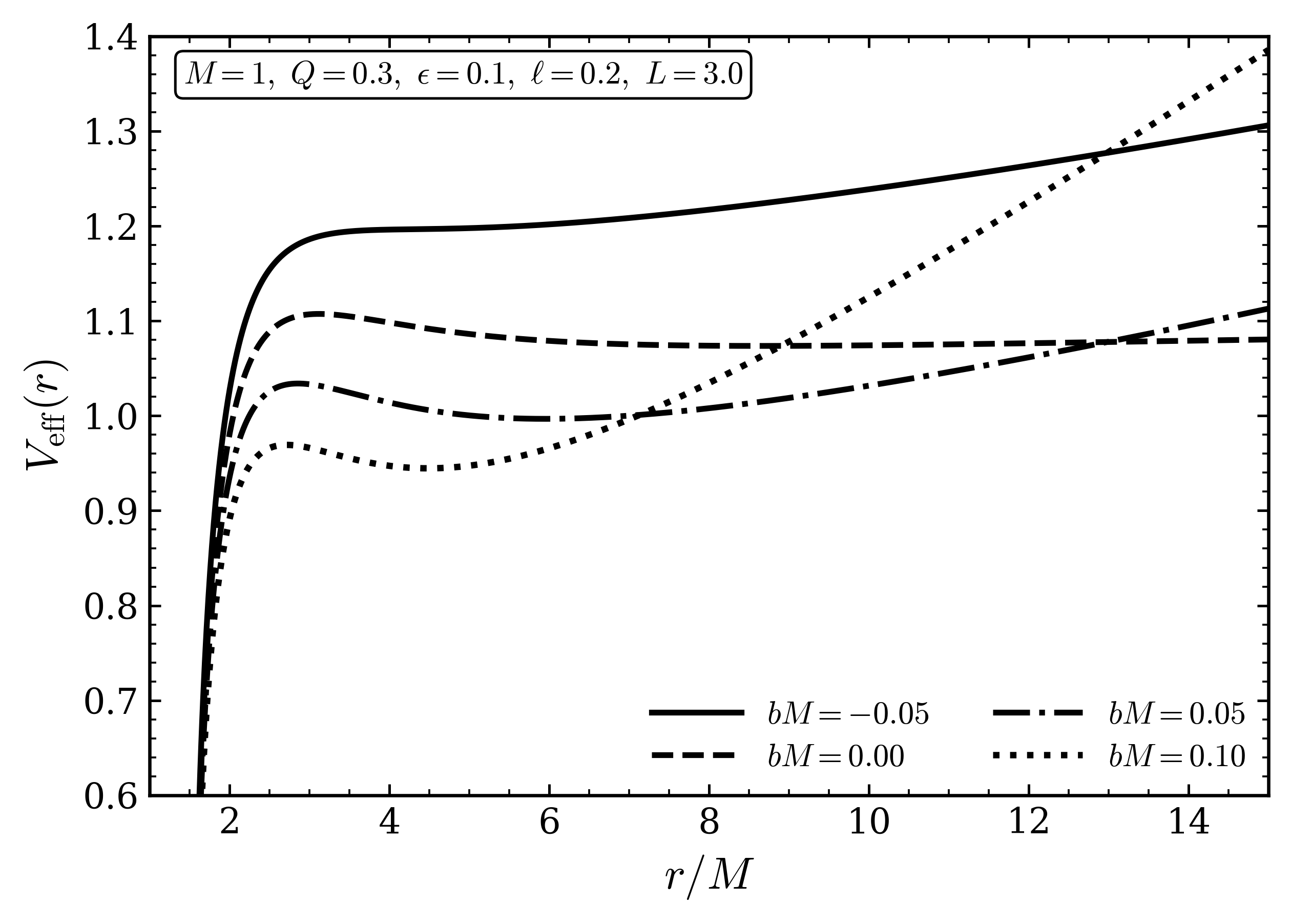
Figure 4 displays the effective potential for different values of the magnetic coupling . The potential contains two physically distinct contributions. The first term, , is the electrostatic interaction between the charged particle and the charged KR black hole. For the parameters used in the plot, , so this term is repulsive and is most important close to the compact object. The second contribution is the square-root term, which contains the gravitational redshift and the effective centrifugal barrier through . Since grows with radius, even a small magnetic coupling can strongly modify the mechanical angular momentum at large distances. Positive reduces for fixed canonical , while negative increases it. The magnetic field therefore changes the height and radial location of the potential barrier by altering the balance between centrifugal support, electrostatic repulsion, and gravitational attraction. The shift of the minimum of indicates that the preferred circular-orbit region is sensitive to the sign and magnitude of the Lorentz coupling.
The turning points of the radial motion satisfy
| (60) |
Circular orbits are determined by the simultaneous conditions
| (61) |
where the derivative is taken with respect to at fixed conserved quantities and .
For compactness, define
| (62) |
Differentiating Eq. (54) with respect to and setting the result to zero gives
| (63) |
The last two terms arise from differentiating at fixed and :
| (64) |
For nonzero electric and magnetic couplings, the circular-orbit equations do not generally admit a simple closed-form solution. In the numerical implementation, for each chosen radius we substitute the physical turning-point branch
| (65) |
into Eq. (63). This gives a single nonlinear equation for :
| (66) |
After solving Eq. (66) numerically for , the corresponding specific energy is obtained from Eq. (65). This procedure is equivalent to solving the coupled system and for .
The circular-orbit values of the specific angular momentum and specific energy are shown in Figs. 5 and 6. These two quantities respond differently to the magnetic field because the conserved angular momentum is canonical, whereas the actual azimuthal motion is controlled by the mechanical combination . For a fixed circular orbit, the radial force balance first fixes the mechanical angular momentum needed to counteract gravity and electrostatic repulsion. The canonical angular momentum must then absorb the magnetic vector-potential contribution, so that . This explains why the curves for separate clearly as changes. The separation becomes more pronounced at larger radii because increases outward. By contrast, the specific energy depends on the same magnetic correction only through the square-root combination in Eq. (65); therefore varies more smoothly. Physically, the magnetic field mainly redistributes the angular-momentum budget of the orbit, while the energy is controlled by the combined gravitational redshift, electrostatic interaction, and kinetic support required for circular motion.


The stability of circular orbits can be analyzed either through the effective potential or, equivalently, through the radial function. A stable circular orbit corresponds to a local minimum of the effective potential,
| (67) |
The equivalent stability condition in terms of the radial function has the opposite sign. Indeed,
| (68) |
and for the physical branch at a circular orbit one obtains
| (69) |
where primes denote differentiation with respect to at fixed conserved quantities. Since outside the horizon, the condition is equivalent to
| (70) |
The marginally stable circular orbit is determined by
| (71) |
and corresponds to the ISCO in the appropriate parameter range.
The marginally stable orbit is obtained from Eq. (71). The dependence of on and is summarized in Figs. 7 and 8, with the corresponding numerical values reported in Table 2. The ISCO is a sensitive probe of the competition between gravity, electric repulsion, centrifugal support, and the magnetic Lorentz interaction. Increasing changes the metric normalization and reduces the event-horizon radius for the fixed charge used here. As a result, the stable-orbit region moves closer to the black hole, and decreases in the parameter interval shown. The magnetic coupling then adds a second control parameter. Because enters through , it directly changes the mechanical angular momentum that appears in the radial potential. In the present parameter set, switching on the magnetic interaction shifts the ISCO inward relative to the non-magnetized case, with the strongest inward shift occurring for positive . This indicates that the Lorentz force effectively helps the particle maintain stable circular motion at smaller radii by modifying the centrifugal balance. Thus, the KR deformation fixes the background gravitational scale, while the magnetic coupling controls how deeply charged particles can remain on stable circular orbits within that background.


| 0.0 | -0.05 | 4.924024 | 1.187846 | 4.486104 | 0.118744 |
| 0.0 | 0.00 | 5.861913 | 0.943281 | 3.370828 | 0.069162 |
| 0.0 | 0.05 | 4.607413 | 0.843499 | 3.260279 | 0.070705 |
| 0.0 | 0.10 | 3.908894 | 0.788564 | 3.408998 | 0.078291 |
| 0.1 | -0.05 | 4.613557 | 1.184140 | 3.693319 | 0.120992 |
| 0.1 | 0.00 | 5.228147 | 0.994118 | 3.011006 | 0.077514 |
| 0.1 | 0.05 | 4.275870 | 0.904598 | 2.940426 | 0.078445 |
| 0.1 | 0.10 | 3.657231 | 0.851334 | 3.055029 | 0.086191 |
| 0.2 | -0.05 | 4.253802 | 1.201170 | 3.032794 | 0.124623 |
| 0.2 | 0.00 | 4.579763 | 1.054007 | 2.646078 | 0.088475 |
| 0.2 | 0.05 | 3.880964 | 0.974474 | 2.609944 | 0.089065 |
| 0.2 | 0.10 | 3.360648 | 0.923260 | 2.697327 | 0.096709 |
| 0.3 | -0.05 | 3.812564 | 1.239676 | 2.467302 | 0.131642 |
| 0.3 | 0.00 | 3.906242 | 1.125832 | 2.272580 | 0.103792 |
| 0.3 | 0.05 | 3.412712 | 1.055803 | 2.262862 | 0.104425 |
| 0.3 | 0.10 | 3.003532 | 1.007004 | 2.328608 | 0.111728 |
The numerical values emphasize the size of these effects. In the non-magnetized case, the ISCO decreases from at to at . This change is not only a coordinate displacement; it reflects a genuine modification of the radial stability condition caused by the KR deformation of . At fixed , the magnetic coupling further moves the ISCO from for to for . The corresponding physical angular velocity increases as the orbit moves inward, as expected for a smaller stable circular radius. Therefore, even though the magnetic field is treated as a test field and does not backreact on the metric, its Lorentz force can significantly affect the particle-dynamical observables. This makes and useful diagnostics for separating the geometrical effect of the KR parameter from the electromagnetic effect of the external magnetic field.
As a consistency check, in the neutral and non-magnetized limit and , the equations reduce to the standard geodesic relations
| (72) |
and
| (73) |
For neutral circular geodesics, one obtains
| (74) |
These expressions are recovered from the general charged-particle equations when the electric and magnetic interactions are switched off.
Therefore, the KR parameter , the black-hole charge parameter , the particle’s specific charge , and the magnetic coupling jointly modify the effective potential, the allowed region of motion, the circular-orbit structure, and the stability properties of charged particles around the charged KR black hole.
III Frequencies of quasi-periodic oscillations
In this section, we derive the fundamental frequencies of charged-particle motion around the charged KR black hole in the presence of the source-free numerical magnetic field. These frequencies are then used for the QPO analysis within the relativistic precession model.
We consider equatorial circular motion with four-velocity
| (75) |
The normalization condition gives
| (76) |
where the second equality is written on the equatorial plane . Thus, timelike circular motion requires
| (77) |
The orbital angular velocity is determined from the radial component of the Lorentz-force equation,
| (78) |
For the charged KR spacetime with
| (79) |
one has, on the equatorial plane,
| (80) |
With the magnetic coupling parameter , the radial force-balance equation becomes
| (81) |
Therefore, the orbital frequency is obtained as the physical root of
| (82) |
The physical branch is chosen so that it reduces to the neutral Keplerian frequency when :
| (83) |
For nonzero electric and magnetic couplings, Eq. (82) contains both the Coulomb contribution from the charged KR black hole and the Larmor-type correction generated by the external magnetic field. In what follows, the coordinate-time orbital frequency is denoted by . The corresponding physically normalized frequency is obtained later by the same asymptotic time normalization used in Eq. (94). This convention keeps the notation consistent with the previous subsection, where coordinate-time conserved quantities are used in the equations of motion and physical frequencies are obtained only after the rescaling .

Figure 9 shows the radial behavior of the generalized Keplerian frequency. In the plot we use the compact label ; the physical frequency measured by an asymptotic observer is obtained through the normalization . The overall decrease of with increasing radius is a direct consequence of the weakening gravitational attraction far from the compact object. Close to the black hole, however, the orbital frequency is noticeably modified by the combined action of the electric and magnetic interactions. The electric charge of the spacetime enters through the Coulomb term , whereas the magnetic field changes the radial force balance through the term . Since is the numerical solution of the source-free Maxwell equation in the KR geometry, the magnetic correction is not an ad hoc shift but a self-consistent response of the circular dynamics to the external field. Thus the azimuthal period of a charged particle near the compact object is determined not only by gravity, but also by the interplay between Coulomb and Lorentz forces.
The specific energy and angular momentum of the circular orbit are then written as
| (84) |
The radial and vertical epicyclic frequencies are obtained by perturbing the motion around the circular orbit. To avoid confusion with the energy effective potential introduced in the previous subsection, we denote the auxiliary epicyclic potential by :
| (85) |
This quantity is not a second definition of ; it is only a compact form of the four-velocity normalization used for deriving the epicyclic frequencies. On the equatorial plane it is equivalent to the radial function introduced earlier, up to the same circular-orbit conditions. At a circular orbit,
| (86) |
In Eq. (85), the same specific quantities , , , and are used as in the previous subsection. In particular, , and on the equatorial plane this reduces to . Therefore the mechanical angular-momentum combination is consistently
the same quantity that appears in the effective potential and in the radial function . Small perturbations,
| (87) |
satisfy
| (88) |
The epicyclic frequencies measured with respect to the coordinate time are
| (89) |
For the present KR geometry, the radial epicyclic frequency becomes
| (90) |
where
| (91) |
The magnetic terms contain and , which are evaluated from the numerical solution of the source-free Maxwell equation.

Figure 10 displays the radial epicyclic frequency, which governs the oscillation of a particle under small radial displacements from a circular orbit. As in Fig. 9, the plot label is written compactly as ; the physical frequency is . Unlike , the radial frequency is not simply a measure of orbital motion; it is a direct indicator of dynamical stability. When , a radially perturbed particle executes stable harmonic oscillations around the reference orbit. As the orbit approaches the strong-gravity region, decreases and eventually vanishes. This condition is equivalent to the marginal-stability condition used earlier. Therefore, identifies the ISCO, while the region with imaginary corresponds to radially unstable circular motion.
The shape of the curves in Fig. 10 also shows how the magnetic coupling modifies the radial stability of the orbit. Since the magnetic terms in Eq. (90) contain both a linear contribution in and a quadratic contribution in , the external field affects not only the orbital frequency itself but also the response of the system to radial perturbations. In physical terms, the magnetic field changes how efficiently centrifugal support can balance the combined gravitational and electrostatic attraction. Consequently, the radius at which goes to zero shifts with , indicating that the external magnetic field can move the boundary between stable and unstable charged-particle orbits.
The vertical epicyclic frequency takes the compact form
| (92) |
In the absence of magnetic interaction, , spherical symmetry gives
| (93) |
Since the KR metric is not asymptotically normalized in the usual Minkowskian form, the physical frequencies are defined with respect to
Thus,
| (94) |
The corresponding frequencies in hertz are
| (95) |
where denotes the dimensionless frequency obtained in geometrized units.
For the relativistic precession model, the observed QPO frequencies are identified with the physically normalized frequencies,
| (96) |
Equivalently, in angular-frequency notation,
These quantities are then compared with the observed upper and lower QPO frequencies.
The above analysis shows that the KR parameter, the electric charge, and the external magnetic field all enter the QPO problem through well-defined and physically distinct mechanisms. The KR deformation modifies the background geometry and the asymptotic normalization of time, the electric field changes the force balance through the Coulomb interaction, and the source-free magnetic field affects both the orbital frequency and the radial stability via , , and . Therefore, even before fitting any observational data, the fundamental frequencies already encode a nontrivial fingerprint of the KR spacetime and its electromagnetic environment. This makes the pair particularly useful for QPO studies, since after the common physical-time rescaling these two frequencies directly determine the relativistic-precession observables and .
III.1 Markov chain Monte Carlo analysis for quasi-periodic oscillations
We constrain the charged KR black-hole model using the observed twin-peak QPO frequencies of GRO J1655–40, XTE J1550–564, and M82 X-1. Within the relativistic precession model, the theoretical upper and lower frequencies are identified as
| (97) |
where and are calculated from Eqs. (95) and (96) at the QPO emission radius .
The observational frequencies used in the likelihood are summarized in Table 3. The numerical values correspond to the QPO pairs adopted in the present analysis, while the cited observational studies report the corresponding twin-peak detections [85, 74].
| Source | Reference | ||
| GRO J1655–40 | [85] | ||
| XTE J1550–564 | [85] | ||
| M82 X-1 | [74] |
For each source, the observational data vector is written as
| (98) |
To keep the notation identical to that used in the corner plots, the sampled parameter vector is defined as
| (99) |
where is the black-hole mass, is the dimensionless black-hole charge, is the Lorentz-violating parameter, is the particle specific charge, is the dimensionless magnetic coupling, and is the dimensionless QPO emission radius.
The posterior probability density is given by Bayes’ theorem,
| (100) |
where is the likelihood, is the prior, and is the Bayesian evidence.
Assuming independent Gaussian errors for the two observed frequencies, the log-likelihood is
| (101) |
The priors are restricted to the physically allowed region. In particular, the sampled points must satisfy
| (102) |
together with the conditions that the orbit lies outside the event horizon, remains timelike, and has a real radial epicyclic frequency. For Gaussian priors, the logarithm of the prior probability is written as
| (103) |
inside the imposed parameter intervals, while outside the allowed region.
The posterior distributions were sampled with the affine-invariant ensemble sampler implemented in the emcee package [39]. For each source, we used 24 walkers. For GRO J1655–40 and M82 X-1, the chains were evolved for steps, and the first steps were discarded as burn-in. For XTE J1550–564, the chains were evolved for steps, and the first steps were discarded as burn-in. The remaining chains were thinned by retaining every fifth sample for GRO J1655–40 and M82 X-1, and every 25th sample for XTE J1550–564. The thinning was used only to reduce the storage size of the posterior samples and does not affect the sampling procedure itself.
For each parameter, the reported central value is the median of the marginalized posterior, while the lower and upper uncertainties are obtained from the 16th and 84th percentiles:
| (104) |
| Source | ||||||
| GRO J1655–40 | ||||||
| XTE J1550–564 | ||||||
| M82 X-1 |
The MCMC analysis was performed using Gaussian priors for the six model parameters. The mean values and standard deviations of these priors are listed in Table 4. The priors were obtained from a preliminary scan of the physically admissible parameter space, where the horizon condition, timelike circular motion, and real epicyclic frequencies were imposed. Since the model contains six free parameters, whereas each source provides two observed QPO frequencies, the adopted priors help restrict the sampling to physically meaningful regions of the parameter space. Consequently, the posterior constraints should be interpreted within the adopted model and prior assumptions.
Because the posterior constraints can be sensitive to the adopted priors, especially in a multi-parameter model constrained by two QPO frequencies, the prior choices are explicitly reported for transparency.
The marginalized posterior constraints obtained from the MCMC samples are summarized in Table 5, while the corresponding one- and two-dimensional posterior distributions are shown in Figs. 11, 12, and 13.
| Parameter | GRO J1655–40 | XTE J1550–564 | M82 X-1 |
Figures 11–13 display the one-dimensional marginalized distributions along the diagonal and the pairwise joint posterior distributions in the off-diagonal panels. The vertical and horizontal lines indicate the posterior median values.
| Source | Acceptance fraction | range | Final samples | |
| GRO J1655–40 | 0.4807 | 73.87–110.51 | 90.49 | 38400 |
| XTE J1550–564 | 0.5043 | 65.11–84.00 | 1190.48 | 76800 |
| M82 X-1 | 0.5025 | 68.77–82.70 | 120.92 | 38400 |
The convergence of the chains was checked using the mean acceptance fraction and the integrated autocorrelation time. As shown in Table 6, the mean acceptance fractions lie in the range –, indicating efficient sampling. The ratio is larger than for all sources, showing that the chains are sufficiently longer than the corresponding autocorrelation times. Therefore, the marginalized posterior constraints reported in Table 5 can be estimated reliably within the adopted model and prior ranges.


The corner plots reveal several parameter correlations. In particular, the magnetic coupling is correlated with the mass and the orbital radius, while and exhibit an appreciable anti-correlation for XTE J1550–564 and GRO J1655–40. These correlations reflect the fact that the observed QPO pair constrains combinations of the model parameters more strongly than each parameter separately. Consequently, the quoted intervals should be interpreted within the adopted six-parameter model and prior ranges.
| Source | |||||
| GRO J1655–40 | 451.00 | 450.9703 | 298.00 | 298.0015 | |
| XTE J1550–564 | 276.00 | 276.0261 | 184.00 | 183.8560 | |
| M82 X-1 | 5.07 | 5.0689 | 3.32 | 3.3178 |
Table 7 compares the observed QPO frequencies with the best-fit theoretical values obtained in the present model. The very small residuals in Table 7 show that the model can reproduce the adopted QPO pairs at the best-fit points. Since the model contains several free parameters, these small values should be viewed as a consistency check of the frequency reconstruction rather than as an independent model-selection criterion.
IV Conclusion
In this work, we investigated charged-particle dynamics and quasi-periodic oscillations around a Reissner–Nordström-like black hole in KR gravity in the presence of an external magnetic test field. The KR background introduces a Lorentz-violating parameter, which modifies the metric function, the horizon structure, the circular-orbit properties, and the characteristic frequencies of particle motion. A central point of the present analysis is that the magnetic field was not imposed by using the standard Wald-type prescription. Instead, it was obtained from the source-free Maxwell equation on the charged KR background. This makes the magnetic configuration consistent with the modified geometry and its asymptotic structure.
We derived the equations of motion for charged test particles, constructed the effective potential, and analyzed the conditions for circular orbits and their stability. The results show that the black-hole charge, the KR parameter, the specific charge of the particle, and the magnetic coupling jointly determine the behavior of charged-particle motion. The magnetic field modifies the mechanical angular momentum of the particle, while the KR parameter changes the gravitational background itself. Therefore, the ISCO and the orbital frequency are affected by the combined influence of the geometrical deformation and the electromagnetic interaction. The ISCO results summarized in Table 2 show that the stable-orbit region is sensitive to both the KR deformation and the magnetic coupling, indicating that electromagnetic effects may remain important even in the test-field approximation.
We also derived the orbital and radial epicyclic frequencies and applied them to high-frequency QPOs within the relativistic precession model. In this framework, the upper QPO frequency is associated with the orbital frequency, while the lower QPO frequency is related to the periastron-precession frequency. Since these frequencies are generated in the strong-field region close to the compact object, they provide a useful phenomenological probe of the spacetime geometry and the surrounding electromagnetic environment.
The observed QPO data used in the statistical analysis are listed in Table 3. These data were used for the three sources GRO J1655–40, XTE J1550–564, and M82 X-1. The model parameters were constrained by means of a Markov chain Monte Carlo analysis. The adopted Gaussian priors are presented in Table 4, while the corresponding posterior constraints are summarized in Table 5. This structure makes the statistical analysis transparent: the observational input is given separately, the prior assumptions are explicitly stated, and the final parameter constraints are reported independently in the posterior table.
According to the posterior constraints in Table 5, the charged KR black-hole model with an external magnetic test field can reproduce the observed QPO pairs of all three sources within the adopted model and prior ranges. The inferred masses remain consistent with the expected astrophysical character of the corresponding compact objects. The posterior distributions also indicate that the QPO data are compatible with nonzero values of the charge and KR parameters in the considered framework. In addition, the preferred emission radii reported in Table 5 lie in the strong-field region, where the orbital and radial epicyclic frequencies are particularly sensitive to changes in the background geometry.
The convergence diagnostics reported in Table 6 support the reliability of the sampling procedure. The acceptance fractions and integrated autocorrelation times show that the chains sample the posterior distributions efficiently for the three sources. The corresponding corner plots illustrate the marginalized posterior distributions and the correlations among the model parameters. These correlations are physically expected, because the observed QPO frequencies depend simultaneously on the mass, charge, KR parameter, magnetic coupling, specific particle charge, and emission radius.
Overall, the present results suggest that QPO observations can provide meaningful phenomenological constraints on Lorentz-violating black-hole spacetimes when the effects of charge and magnetic fields are included. The analysis also shows that the KR deformation and the magnetic interaction should not be treated as completely independent observational effects, since both can influence the same strong-field frequencies. Thus, the combined study of particle dynamics, ISCO behavior, and QPO frequencies offers a useful way to test modified black-hole geometries in astrophysical environments.
At the same time, the obtained constraints should be interpreted with appropriate care. The model contains several free parameters, whereas each source provides only a limited number of observed QPO frequencies. Therefore, the posterior constraints depend on the adopted priors and on the assumptions of the relativistic precession model. Moreover, the magnetic field was treated in the test-field approximation, and the effects of plasma dynamics, detailed accretion-disk structure, radiation transport, magnetic-field backreaction, and black-hole spin were not included.
Future work may extend the present analysis to rotating KR black holes and to more realistic disk and plasma models. It would also be useful to combine QPO constraints with other observables, such as black-hole shadows, continuum spectra, and iron-line profiles. Such a combined approach may help reduce parameter degeneracies and provide stronger observational tests of Lorentz-violating gravity in the strong-field regime.
Acknowledgments
S.M. gratefully acknowledges support from Grant FZ-20200929385 of the Agency of Innovative Developments of the Republic of Uzbekistan.
References
- [1] (2024) Physical Review D 109, pp. 104074. External Links: Document, Link Cited by: §I.
- [2] (2015) Physical Review D 91, pp. 052003. External Links: Document, Link Cited by: §I.
- [3] (2001) A precise determination of black hole spin in gro j1655–40. Astronomy and Astrophysics 374, pp. L19–L20. External Links: Document, Link Cited by: §I.
- [4] (2026) Physics of the Dark Universe 52, pp. 102311. External Links: Document, Link Cited by: §I.
- [5] (2026) Physics of the Dark Universe 52, pp. 102315. External Links: Document, Link Cited by: §I.
- [6] (2026) Imprints of modmax electrodynamics on particle dynamics and thermodynamic properties of kalb–ramond ads black holes. Int. J Geom. Meth. Mod. Phys., pp. 2650130. Note: Online first External Links: Document, Link Cited by: §I.
- [7] (2026) Geodesic structure, perturbative dynamics and thermal properties of black hole in kalb–ramond gravity. Mod. Phys. Lett. A 41 (12n13), pp. 2650061. External Links: Document, Link Cited by: §I.
- [8] (2025) Particle dynamics and thermal properties in kalb–ramond modmax black holes: theoretical predictions for observational tests of exotic physics. Phys. Dark Univ. 50, pp. 102076. External Links: ISSN 2212-6864, Document, Link Cited by: §I.
- [9] (2026) Gravitational dynamics and shadow formation in magnetized black hole solutions coupled with a cloud of strings. Annals of Physics 490, pp. 170475. External Links: ISSN 0003-4916, Document, Link Cited by: §I.
- [10] (2024) Geodesics structure and deflection angle of electrically charged black holes in gravity with a background kalb–ramond field. Eur. Phys. J C 84 (8), pp. 825. External Links: Document Cited by: §I.
- [11] (2002) Motion of charged particles around a rotating black hole in a magnetic field. Monthly Notices of the Royal Astronomical Society 336, pp. 241–248. External Links: Document, Link Cited by: §I.
- [12] (1998) Tests of quantum gravity from observations of gamma-ray bursts. Nature 393, pp. 763–765. External Links: Document, Link Cited by: §I.
- [13] (2025) European Physical Journal C 85, pp. 633. External Links: Document, Link Cited by: §I.
- [14] (2023) Physical Review D 108, pp. 024045. External Links: Document, Link Cited by: §I.
- [15] (2012) Testing the kerr black hole hypothesis. Journal of Cosmology and Astroparticle Physics 2012, pp. 014. External Links: Document, Link Cited by: §I.
- [16] (2025) Effects of qcd-based equation of state on properties of compact stars in gravity’s rainbow. European Physical Journal C 85 (10), pp. . Note: Cited by: 1; All Open Access; Gold Open Access; Green Open Access External Links: Document, Link Cited by: §I.
- [17] (2025) Existence of quark stars in gravity’s rainbow: the significance of strongly interacting quark matter. Chinese Physics C 49 (12), pp. . Note: Cited by: 1; All Open Access; Hybrid Gold Open Access External Links: Document, Link Cited by: §I.
- [18] (2012) High-frequency quasi-periodic oscillations in black hole binaries. Monthly Notices of the Royal Astronomical Society 426, pp. 1701–1709. External Links: Document, Link Cited by: §I.
- [19] (2020) Physical Review D 101, pp. 124024. External Links: Document, Link Cited by: §I.
- [20] (2005) Noncommutative-field-theory analysis of bounds on lorentz violation. Physical Review D 72, pp. 025010. External Links: Document, Link Cited by: §I.
- [21] (1977) Electromagnetic extraction of energy from kerr black holes. Monthly Notices of the Royal Astronomical Society 179, pp. 433–456. External Links: Document, Link Cited by: §I.
- [22] (2005) Spontaneous lorentz violation, nambu-goldstone modes, and gravity. Physical Review D 71, pp. 065008. External Links: Document, Link Cited by: §I.
- [23] (2023) Physical Review D 108, pp. 044063. External Links: Document, Link Cited by: §I.
- [24] (2024) Electromagnetic field and chaotic charged-particle motion around hairy black holes in horndeski gravity. European Physical Journal C 84, pp. 435. External Links: Document, 2404.19225, Link Cited by: §I.
- [25] (2015) Cosmological implications of bumblebee vector models. Physical Review D 91, pp. 104007. External Links: Document, Link Cited by: §I.
- [26] (2004) Lorentz-violating vector fields slow the universe down. Physical Review D 70, pp. 123525. External Links: Document, Link Cited by: §I.
- [27] (2018) Exact schwarzschild-like solution in a bumblebee gravity model. Physical Review D 97, pp. 104001. External Links: Document, Link Cited by: §I.
- [28] (1998) Lorentz-violating extension of the standard model. Physical Review D 58, pp. 116002. External Links: Document, Link Cited by: §I.
- [29] (2025) European Physical Journal C 85, pp. 1141. External Links: Document, Link Cited by: §I.
- [30] (2025) Physical Review D 112, pp. 104018. External Links: Document, Link Cited by: §I.
- [31] (2025) Physical Review D 112, pp. 124018. External Links: Document, Link Cited by: §I.
- [32] (2024) Journal of High Energy Astrophysics 43, pp. 51. External Links: Document, Link Cited by: §I.
- [33] (2026) Thermodynamics around new wormhole solutions in extended teleparallel gravity coupled with euler-heisenberg electrodynamics. European Physical Journal Plus 141 (5), pp. . Note: Cited by: 0 External Links: Document, Link Cited by: §I.
- [34] (2026) Testing strong gravitational field using the johannsen–psaltis metric: bondi–hoyle–lyttleton accretion model and qpo studies. Annals of Physics 486, pp. . Note: Cited by: 3 External Links: Document, Link Cited by: §I.
- [35] (2024) Electrically charged black holes in gravity with a background kalb–ramond field. European Physical Journal C 84, pp. 798. External Links: Document, 2310.13555, Link Cited by: §I, §II.
- [36] (2026) Holographic dark energy as a source for slowly rotating wormholes: implications for null geodesics and shadows. Physics Letters, Section B: Nuclear, Elementary Particle and High-Energy Physics 878, pp. . Note: Cited by: 0; All Open Access; Gold Open Access; Green Open Access External Links: Document, Link Cited by: §I.
- [37] (2021) First m87 event horizon telescope results. vii. polarization of the ring. The Astrophysical Journal Letters 910, pp. 13. External Links: Document, Link Cited by: §I.
- [38] (2015) The physics of accretion onto black holes. Springer New York, New York. External Links: Document, Link Cited by: §I.
- [39] (2013) Emcee: the MCMC hammer. Publications of the Astronomical Society of the Pacific 125 (925), pp. 306–312. External Links: Document Cited by: §I, §III.1.
- [40] (2010) Motion of charged particles near weakly magnetized schwarzschild black hole. Physical Review D 82, pp. 084034. External Links: Document, 1008.2985, Link Cited by: §I.
- [41] (2026) Stability analysis of charged acoustic thin-shell wormholes. Nuclear Physics B 1025, pp. . Note: Cited by: 0; All Open Access; Gold Open Access; Green Open Access External Links: Document, Link Cited by: §I.
- [42] (2026) Analyzing deformed-ads thin-shell wormholes with global monopole and quintessence. Physics of the Dark Universe 52, pp. . Note: Cited by: 2 External Links: Document, Link Cited by: §I.
- [43] (2025) European Physical Journal C 85, pp. 95. External Links: Document, Link Cited by: §I.
- [44] (2025) Journal of Cosmology and Astroparticle Physics 2025, pp. 035. External Links: Document, Link Cited by: §I.
- [45] (2026) Journal of High Energy Physics 2026, pp. 20. External Links: Document, Link Cited by: §I.
- [46] (2024) European Physical Journal C 84, pp. 964. External Links: Document, Link Cited by: §I.
- [47] (2025) European Physical Journal C 85, pp. 126. External Links: Document, Link Cited by: §I.
- [48] (2025) Black holes surrounded by pfdm in kalb-ramond gravity: from thermodynamics to qpo tests. European Physical Journal C 85 (7), pp. . Note: Cited by: 27; All Open Access; Gold Open Access; Green Open Access External Links: Document, Link Cited by: §I.
- [49] (2025) Radiative properties and qpos around charged black hole in kalb–ramond gravity. European Physical Journal C 85 (2), pp. . Note: Cited by: 50; All Open Access; Gold Open Access; Green Open Access External Links: Document, Link Cited by: §I.
- [50] (2024) European Physical Journal C 84, pp. 1257. External Links: Document, Link Cited by: §I.
- [51] (2025) European Physical Journal C 85, pp. 557. External Links: Document, Link Cited by: §I.
- [52] (1974) Classical direct interstring action. Physical Review D 9, pp. 2273–2284. External Links: Document, Link Cited by: §I.
- [53] (2008) Lorentz violating inflation. Journal of Cosmology and Astroparticle Physics 2008, pp. 034. External Links: Document, Link Cited by: §I.
- [54] (2026) Nonmetric geometry and its role in the isotropization of self-gravitating stellar models. Nuclear Physics B 1022, pp. . Note: Cited by: 3; All Open Access; Gold Open Access; Green Open Access External Links: Document, Link Cited by: §I.
- [55] (2026) Quasi-periodic oscillations in rotating simpson–visser black holes in stvg. European Physical Journal C 86 (6), pp. . Note: Cited by: 0; All Open Access; Gold Open Access; Green Open Access External Links: Document, Link Cited by: §I.
- [56] (2015) Classical and Quantum Gravity 32, pp. 165009. External Links: Document, Link Cited by: §I.
- [57] (1989) Gravitational phenomenology in higher-dimensional theories and strings. Physical Review D 40, pp. 1886. External Links: Document, Link Cited by: §I.
- [58] (1989) Spontaneous breaking of lorentz symmetry in string theory. Physical Review D 39, pp. 683–685. External Links: Document, Link Cited by: §I.
- [59] (2004) Gravity, lorentz violation, and the standard model. Physical Review D 69, pp. 105009. External Links: Document, Link Cited by: §I.
- [60] (2026) Physical Review D 113, pp. 044003. External Links: Document, Link Cited by: §I.
- [61] (2025) Physical Review D 112, pp. 064031. External Links: Document, Link Cited by: §I.
- [62] (2023) Journal of Cosmology and Astroparticle Physics 2023, pp. 096. External Links: Document, Link Cited by: §I.
- [63] (2023) Physics of the Dark Universe 42, pp. 101311. External Links: Document, Link Cited by: §I.
- [64] (2026) Two types of quasinormal modes of casadio-fabbri-mazzacurati brane-world black holes. Nuclear Physics B 1029, pp. . Note: Cited by: 0; All Open Access; Gold Open Access; Green Open Access External Links: Document, Link Cited by: §I.
- [65] (2026) A first-order eikonal framework for quasinormal modes, shadows, strong lensing, and grey-body factors in a scalarized black-hole metric. Annals of Physics 491, pp. . Note: Cited by: 0; All Open Access; Green Open Access External Links: Document, Link Cited by: §I.
- [66] (2021) Physical Review D 103, pp. 044002. External Links: Document, Link Cited by: §I.
- [67] (2005) Modern tests of lorentz invariance. Living Reviews in Relativity 8, pp. 5. External Links: Document, Link Cited by: §I.
- [68] (2025) Theoretical study of strong gravitational lensing around dyonic modmax black hole: constraints from eht observations. Chinese Physics C 49 (12), pp. . Note: Cited by: 3 External Links: Document, Link Cited by: §I.
- [69] (2025) QPOs tests and circular motions of charged particles around magnetized bocharova–bronnikov–melnikov–bekenstein black holes. European Physical Journal C 85 (5), pp. . Note: Cited by: 8; All Open Access; Gold Open Access; Green Open Access External Links: Document, Link Cited by: §I.
- [70] (2026) Probing quantum corrected kazakov–solodukhin black holes through qpos and thin accretion disks. European Physical Journal C 86 (5), pp. . Note: Cited by: 0; All Open Access; Gold Open Access; Green Open Access External Links: Document, Link Cited by: §I.
- [71] (2025) European Physical Journal C 85, pp. 1029. External Links: Document, Link Cited by: §I.
- [72] (2025) QPOs from charged particles around charged black holes in stvg. European Physical Journal C 85 (9), pp. . Note: Cited by: 9; All Open Access; Gold Open Access; Green Open Access External Links: Document, Link Cited by: §I.
- [73] (2021) 3+1 formulation of the standard-model extension gravity sector. Physical Review D 103, pp. 044010. External Links: Document, Link Cited by: §I.
- [74] (2014) A 400-solar-mass black hole in the galaxy M82. Nature 513, pp. 74–76. External Links: Document Cited by: §I, §III.1, Table 3.
- [75] (2025) Physical Review D 111, pp. 124005. External Links: Document, Link Cited by: §I.
- [76] (2008) Probes and tests of strong-field gravity with observations in the electromagnetic spectrum. Living Reviews in Relativity 11, pp. 9. External Links: Document, Link Cited by: §I.
- [77] (2008) Monthly Notices of the Royal Astronomical Society 389, pp. 27. External Links: Document, Link Cited by: §I.
- [78] (2025) Gravitational lensing by black holes surrounded by pfdm in kalb-ramond gravity in plasma medium. Physics of the Dark Universe 50, pp. . Note: Cited by: 8 External Links: Document, Link Cited by: §I.
- [79] (2026) Astrophysical signatures of rotating kazakov-solodukhin black holes: shadows and constraints from eht observations. Nuclear Physics B 1022, pp. . Note: Cited by: 8; All Open Access; Gold Open Access; Green Open Access External Links: Document, Link Cited by: §I.
- [80] (2025) QPO tests and charged particles around regular ayón-beato-garcia black holes. Physics of the Dark Universe 50, pp. . Note: Cited by: 7 External Links: Document, Link Cited by: §I.
- [81] (2026) Weak gravitational lensing by charged black holes in stvg: constraints from the sloan lens acs survey. Annals of Physics 488, pp. . Note: Cited by: 7 External Links: Document, Link Cited by: §I.
- [82] (2026) Gravitational lensing around quantum-corrected black holes within plasma environment. Physics of the Dark Universe 52, pp. . Note: Cited by: 6 External Links: Document, Link Cited by: §I.
- [83] (2026) Magnetic field by current loop in the janis-newman-winicour spacetime. Nuclear Physics B 1024, pp. . Note: Cited by: 1; All Open Access; Gold Open Access; Green Open Access External Links: Document, Link Cited by: §I.
- [84] (1999) RXTE observations of 0.1–300 hz quasi-periodic oscillations in the microquasar GRO J1655-40. The Astrophysical Journal 522, pp. 397–412. External Links: Document Cited by: §I.
- [85] (2002) Evidence for harmonic relationships in the high-frequency quasi-periodic oscillations of XTE J1550-564 and GRO J1655-40. The Astrophysical Journal 580, pp. 1030–1042. External Links: Document Cited by: §I, §III.1, Table 3, Table 3.
- [86] (2025) Black hole surrounded by perfect fluid dark matter in stv gravity: particle dynamics, thermodynamics, gravitational weak lensing and eht tests. European Physical Journal C 85 (9), pp. . Note: Cited by: 4; All Open Access; Gold Open Access; Green Open Access External Links: Document, Link Cited by: §I.
- [87] (2023) The Astrophysical Journal 959, pp. 6. External Links: Document, Link Cited by: §I.
- [88] (2026) Magnetic fields and magnetized particles around black holes in braneworlds. European Physical Journal Plus 141 (5), pp. . Note: Cited by: 0 External Links: Document, Link Cited by: §I.
- [89] (2025) Phantom black holes in f(r,t) gravity: from circular orbits to qpo tests. Physics of the Dark Universe 50, pp. . Note: Cited by: 5 External Links: Document, Link Cited by: §I.
- [90] (2026) Circular motion and qpos near bhs surrounded by dust fields in f(r, t) gravity. Nuclear Physics B 1022, pp. . Note: Cited by: 1; All Open Access; Gold Open Access External Links: Document, Link Cited by: §I.
- [91] (1998) Lense–thirring precession and quasi-periodic oscillations in low-mass x-ray binary systems. The Astrophysical Journal 492, pp. L59–L62. External Links: Document, Link Cited by: §I.
- [92] (2016) European Physical Journal C 76, pp. 32. External Links: Document, Link Cited by: §I.
- [93] (2008) Acta Astronomica 58, pp. 441. External Links: Link Cited by: §I.
- [94] (2013) Astronomy and Astrophysics 552, pp. A10. External Links: Document, Link Cited by: §I.
- [95] (2016) Physical Review D 93, pp. 084012. External Links: Document, Link Cited by: §I.
- [96] (1984) General relativity. University of Chicago Press, Chicago. Cited by: §I.
- [97] (1974) Black hole in a uniform magnetic field. Physical Review D 10, pp. 1680–1685. External Links: Document, Link Cited by: §I.
- [98] (2022) European Physical Journal C 82, pp. 528. External Links: Document, Link Cited by: §I.
- [99] (2026) European Physical Journal C 86, pp. 79. External Links: Document, Link Cited by: §I.
- [100] (2023) Static and spherically symmetric black holes in gravity with a background kalb–ramond field. Physical Review D 108, pp. 124004. External Links: Document, Link Cited by: §I.
- [101] (2013) Physical Review D 87, pp. 084043. External Links: Document, Link Cited by: §I.
- [102] (2025) Physics of the Dark Universe 50, pp. 102127. External Links: Document, Link Cited by: §I.
- [103] (2026) Orbital dynamics and frequency spectra around a black hole with scalar hair. International Journal of Geometric Methods in Modern Physics, pp. . Note: Cited by: 0 External Links: Document, Link Cited by: §I.