On the spherical Blaschke-Lebesgue problem

The classical Blaschke-Lebesgue problem asks which convex bodies of a fixed constant width have the least volume. In the Euclidean plane, Blaschke and Lebesgue independently proved that the area minimizer is the Reuleaux triangle [3, 11]. In higher-dimensional Euclidean space the problem remains open already in dimension three, where the expected minimizers are the Meissner bodies; see, for example, [13] for background and further references. A useful high-dimensional normalization is the effective radius $r(K)$: for a body $K\subset\mathbb{R}^{n}$ of constant width $2$, let $r(K)$ be defined by $\operatorname{vol}_{n}(K)=\operatorname{vol}_{n}(r(K)\mathbb{B}^{n}_{E})$, where $\operatorname{vol}_{n}$ is the Lebesgue measure in $\mathbb{R}^{n}$ and $\mathbb{B}^{n}_{E}$ is the unit Euclidean ball in $\mathbb{R}^{n}$. Further, let $r_{n}$ be the minimum of $r(K)$ over all bodies of constant width $2$ in $\mathbb{R}^{n}$. Evidently, $r_{n}\leq r(\mathbb{B}^{n}_{E})=1$. Schramm proved the non-trivial lower bound

and asked whether $r_{n}$ is bounded away from $1$ in all sufficiently large dimensions [16]. This was recently answered affirmatively by Arman, Bondarenko, Nazarov, Prymak and Radchenko: they constructed, for all sufficiently large $n$, Euclidean bodies of constant width $2$ with effective radius less than $0.891$ [1]. Thus in the Euclidean high-dimensional case there exist bodies of constant width with volume exponentially smaller than that of the ball with the same width, while the exact asymptotic behavior remains unknown and is likely a very hard question to answer.

In this work, we consider the spherical setting. We regard $\mathbb{S}^{n}$ as the unit sphere in $\mathbb{R}^{n+1}$, equipped with its geodesic distance and spherical $n$-measure $\mu_{n}$. Although $\mathbb{S}^{n}$ is a Riemannian manifold and therefore retains many familiar geometric notions, the spherical setting presents genuinely new features. Let $\mathcal{C}_{n}(w)$ denote the class of spherical convex bodies of constant width $w\in(0,\pi)$ in $\mathbb{S}^{n}$. We use the standard definition by supporting hemispheres and the thickness of the narrowest containing lune, see Section 2 for details. The terminology in the literature is not completely uniform: spherical constant width may also be formulated using normal directions, complete bodies, or constant diameter. The equivalences and distinctions among these viewpoints are surveyed by Lassak [9], and the particular complete-body and constant-diameter equivalences needed here are established in [8, 9, 10].

For $K\in\mathcal{C}_{n}(w)$, we define its relative effective radius by

where $\mathbb{B}^{n}(w/2)$ is any geodesic ball of radius $w/2$ in $\mathbb{S}^{n}$. We then set

The normalization is chosen so that a ball of radius $w/2$ has relative effective radius $1$. We note that existence of the limit $\lim_{n\to\infty}\sigma_{n}(w)$ is not known, which is also the case for the Euclidean situation (see [16, Problem 2]).

On $\mathbb{S}^{2}$, the spherical Blaschke-Leichtweiss theorem and its subsequent refinements show that the least-area body of constant width $w$ is a spherical Reuleaux triangle when $0<w\leq\pi/2$, whereas, when $\pi/2\leq w<\pi$, it is the spherical polar of a triangle of width $\pi-w$ [2, 5, 7, 12]. For $w=\pi/2$ this body is the spherical orthant $\mathcal{O}_{2}\mathrel{\mathop{\ordinarycolon}}=\mathbb{S}^{2}\cap\mathbb{R}_{+}^{3}$, so the exact minimizer has area $\pi/2$ which is $1/8$ of the area of the whole $\mathbb{S}^{2}$. Note that the spherical orthant $\mathcal{O}_{n}\mathrel{\mathop{\ordinarycolon}}=\mathbb{S}^{n}\cap\mathbb{R}_{+}^{n+1}$ belongs to $\mathcal{C}_{n}(\pi/2)$ and has the area $1/2^{n+1}$ of the area of the whole $\mathbb{S}^{n}$, so $\overline{\sigma}(\pi/2)\leq\frac{1}{\sqrt{2}}$. Bezdek [2, Conjecture 2.17] conjectured that for every $n\geq 3$, the spherical orthant $\mathcal{O}_{n}$ minimizes $\mu_{n}(K)$ among all $K\in\mathcal{C}_{n}(\pi/2)$.

Our main results treat all fixed widths except this central value $w=\pi/2$. We first define the explicit bases appearing in the bounds. For the lower bound, put

For the upper bound, if $0<w<\pi/2$, set $\theta_{-}(w)\mathrel{\mathop{\ordinarycolon}}=\cos^{-1}\sqrt{\cos w}$ and let $L_{-}(w)$ be the supremum of $(\alpha^{2/3}+\beta^{2/3})^{3/2}$ over all $(\alpha,\beta)\in\mathbb{R}_{+}^{2}$ satisfying

If $\pi/2<w<\pi$, set $\theta_{+}(w)\mathrel{\mathop{\ordinarycolon}}=\cos^{-1}\sqrt{-\cos w}$ and

Finally define

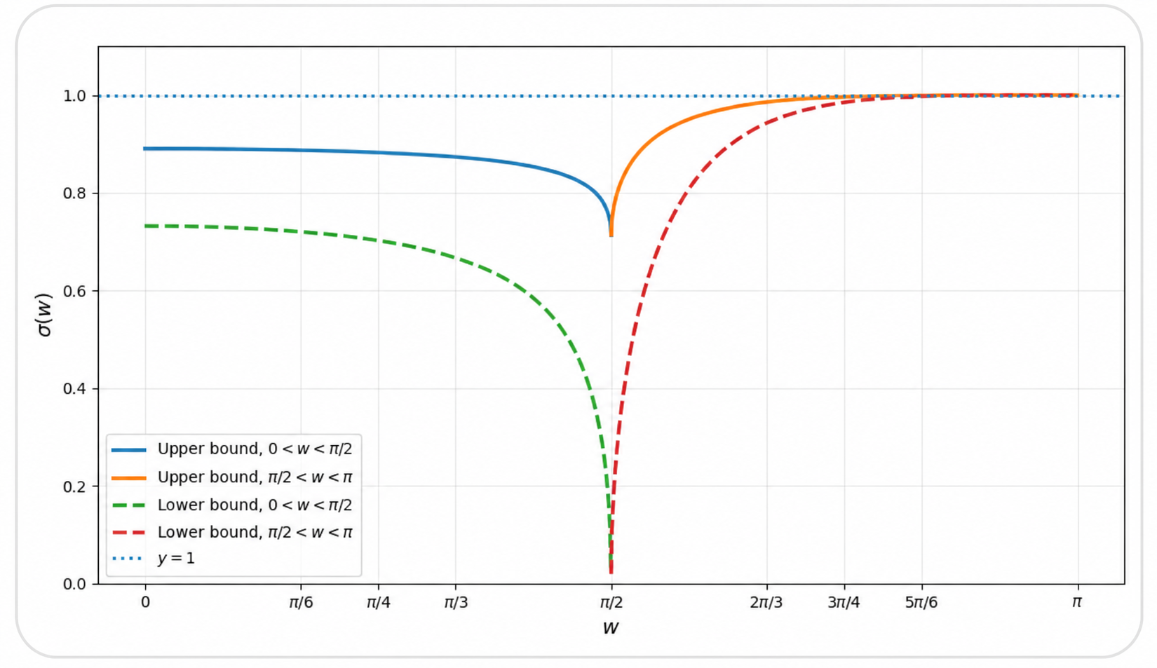
The numerical plot of $\sigma_{\ell}$ and $\sigma_{u}$ is shown in Figure 1. We now state our main result.

Let us describe the proof and the organization of the paper. In Section 2, we recall basic notions of spherical convexity. In Section 3, we prove the upper bound for $0<w<\pi/2$ by constructing a spherical body $M_{w}$ from two orthant pieces on geodesic spheres of radii $\theta_{-}(w)$ and $w-\theta_{-}(w)$, and taking its completion

This is the spherical analogue of the Euclidean construction in [1]. Decomposing $M$ by the signs of its tangential coordinates reduces the exponential contribution to the two-variable optimization in (2). In Section 4, we treat $\pi/2<w<\pi$ using spherical polarity: the polar of a body of constant width $\pi-w$ has constant width $w$. A mixed-orthant covering of the polar body yields the one-dimensional optimization in (3).

For illustration, examples of how our body $M$ looks on $\mathbb{S}^{2}$ are shown in Figure 2. The colors represent different orthants¹¹1A three-dimensional model is available at http://prymak.net/spherical.html. You may also use the slider to change the width..

Finally, Section 5 establishes the lower bound via a spherical version of Schramm’s illumination method, using a ball-containment lemma, spherical Jung-type radius estimates, and the same exponential cap asymptotics. Note that Jung’s estimate does not produce an exponential improvement for $w=\pi/2$. The subexponential estimate resulting from such approach is given by Bezdek in [2, Remark 2.16]. We plan to address this question and show that $\underline{\sigma}(\pi/2)>0$ either in a subsequent version of this work or in a separate work. We remark that an exponential improvement of the lower bound in the case $w=2\pi/3$ would lead to an exponential improvement of the upper bound on Borsuk’s numbers using the method of [15], see also [14, Section 3.2].

We briefly recall the spherical geometric notions used throughout the paper. For more details, we refer the reader to [9]. We regard $\mathbb{S}^{n}$ as the unit sphere in $\mathbb{R}^{n+1}$, endowed with the geodesic distance $d(x,y)=\cos^{-1}\langle x,y\rangle$. For $x\in\mathbb{S}^{n}$, let

be the closed hemisphere centered at $x$; its boundary $\partial H_{x}$ is the corresponding great subsphere. For $x\in\mathbb{S}^{n}$ and $0<r<\pi$, denote the geodesic ball by

For $1\leq j\leq n+1$, denote the vector where the $j$th component is $1$ and the others are $0$ by $e_{j}$. We shall usually fix the north pole $p=e_{1}$ and abbreviate $\mathbb{B}^{n}(r)\mathrel{\mathop{\ordinarycolon}}=\mathbb{B}^{n}(p,r)$. Its spherical measure is $\mu_{n}(\mathbb{B}^{n}(r))=\omega_{n}s_{n}(r)$, where $s_{n}(r)\mathrel{\mathop{\ordinarycolon}}=\int_{0}^{r}\sin^{n-1}t\,dt$ and $\omega_{n}=2\pi^{n/2}/\Gamma(n/2)$ is the surface area of $\mathbb{S}^{n-1}$; see, for example, [4].

If $x,y\in\mathbb{S}^{n}$ are not antipodal, we denote by $[x,y]$ the unique geodesic segment joining them. A set $K\subset\mathbb{S}^{n}$ is spherically convex if it contains no pair of antipodal points and $[x,y]\subset K$ for every $x,y\in K$. In particular, every closed spherical ball of radius $<\pi/2$ is spherically convex, and intersections of spherically convex sets are again spherically convex.

For $x,y\in\mathbb{S}^{n}$, the intersection $L(x,y)\mathrel{\mathop{\ordinarycolon}}=H_{x}\cap H_{y}$ is called a spherical lune. Its thickness is $\Delta(L(x,y))\mathrel{\mathop{\ordinarycolon}}=\pi-d(x,y)$, which is the geodesic distance between the two bounding great subspheres $\partial H_{x}$ and $\partial H_{y}$. Let $K\subset\mathbb{S}^{n}$ be a spherical convex body. A hemisphere $H_{x}$ is said to support $K$ if $K\subset H_{x}$ and $K\cap\partial H_{x}\neq\emptyset$. Given such a supporting hemisphere $H_{x}$, the width of $K$ determined by $H_{x}$ is defined as

We say that $K$ has constant width $w\in(0,\pi)$ if this quantity is equal to $w$ for every supporting hemisphere $H_{x}$.

In addition, write $\mathrm{diam}(K)\mathrel{\mathop{\ordinarycolon}}=\sup\{d(x,y)\mathrel{\mathop{\ordinarycolon}}x,y\in K\}$. The body $K$ is said to have constant diameter $\delta\in(0,\pi)$ if $\mathrm{diam}(K)=\delta$ and, for every $x\in\partial K$, there exists $y\in\partial K$ such that $d(x,y)=\delta$. Finally, we say that $K$ is a complete set of diameter $\delta\in(0,\pi/2)$ if $\mathrm{diam}(K\cup\{x\})>\delta$ for any $x\not\in K$. This is equivalent to

References

• [1] A. Arman, A. Bondarenko, F. Nazarov, A. Prymak, and D. Radchenko, Small volume bodies of constant width, International Mathematics Research Notices 2025 (2025), no. 4, rnaf020, 7 pp. https://doi.org/10.1093/imrn/rnaf020
• [2] K. Bezdek, On a strengthening of the Blaschke–Leichtweiss theorem, Journal of Geometry 114 (2023), no. 1, Paper No. 2, 14 pp. https://doi.org/10.1007/s00022-022-00663-1
• [3] W. Blaschke, Konvexe Bereiche gegebener konstanter Breite und kleinsten Inhalts, Mathematische Annalen 76 (1915), no. 4, 504–513. https://doi.org/10.1007/BF01458221
• [4] K. Böröczky and G. Wintsche, Covering the sphere by equal spherical balls, in Discrete and Computational Geometry: The Goodman–Pollack Festschrift, ed. J. E. Goodman, J. Pach, R. Pollack, and E. Welzl, Algorithms Combin. 25, Springer, Berlin, Heidelberg, 2003, 235–251. https://doi.org/10.1007/978-3-642-55566-4_10
• [5] K. J. Böröczky and Á. Sagmeister, Convex bodies of constant width in spaces of constant curvature and the extremal area of Reuleaux triangles, Studia Scientiarum Mathematicarum Hungarica 59 (2022), no. 3–4, 244–273. https://doi.org/10.1556/012.2022.01528
• [6] B. V. Dekster, The Jung theorem for spherical and hyperbolic spaces, Acta Mathematica Hungarica 67 (1995), no. 4, 315–331. https://doi.org/10.1007/BF01874495
• [7] A. Freyer and Á. Sagmeister, The isominwidth problem on the 2-sphere, Mathematika 72 (2026), e70069. https://doi.org/10.1112/mtk.70069
• [8] H. Han and D. Wu, Constant diameter and constant width of spherical convex bodies, Aequationes Mathematicae 95 (2021), 167–174. https://doi.org/10.1007/s00010-020-00740-3
• [9] M. Lassak, Spherical geometry—a survey on width and thickness of convex bodies, in A. Papadopoulos (ed.), Surveys in Geometry I, Springer, Cham, 2022, 7–47. https://doi.org/10.1007/978-3-030-86695-2_2
• [10] M. Lassak, Complete spherical convex bodies, Journal of Geometry 111 (2020), no. 35. https://doi.org/10.1007/s00022-020-00547-2
• [11] H. Lebesgue, Sur le problème des isopérimètres et sur les domaines de largeur constante, Bulletin de la Société Mathématique de France, C. R. 7 (1914), 72–76.
• [12] K. Leichtweiss, Curves of constant width in the non-Euclidean geometry, Abhandlungen aus dem Mathematischen Seminar der Universität Hamburg 75 (2005), 257–284. https://doi.org/10.1007/BF02942046
• [13] H. Martini, L. Montejano, and D. Oliveros, Bodies of Constant Width: An Introduction to Convex Geometry with Applications, Birkhäuser/Springer, Cham, 2019. https://doi.org/10.1007/978-3-030-03868-7
• [14] G. Kalai, Some old and new problems in combinatorial geometry I: around Borsuk’s problem, Surveys in combinatorics 2015, London Math. Soc. Lecture Note Ser., vol. 424, Cambridge Univ. Press, Cambridge, 2015, pp. 147–174. https://doi.org/10.1017/CBO9781316106853.005
• [15] O. Schramm, Illuminating sets of constant width, Mathematika 35 (1988), 180–189. https://doi.org/10.1112/S0025579300015260
• [16] O. Schramm, On the volume of sets having constant width, Israel Journal of Mathematics 63 (1988), no. 2, 178–182. https://doi.org/10.1007/BF02765037