Latent Actions from Factorized Transition Effects under Agent Ambiguity

Abstract

Latent Action Models (LAMs) learn action-like proxies from observation. However, in multi-object or distractor-rich scenes, observations contain not only agent motion but also distractors, camera dynamics, and background changes, making recovery of the underlying action intrinsically ambiguous without supervision. We argue that the appropriate unsupervised target is therefore not the true action itself, but a state-conditioned compositional summary of the transition effects present in the scene, enabling better action alignment and more effective utilization of action supervision. To this end, we propose a two-stage framework. We first pretrain Observed Transition Factorization (OTF) to discover reusable local transition primitives using a compositional codebook. We then aggregate these primitives into compact state-conditioned latent actions, instantiated as OTF-LAM-Pixel under the standard inverse–forward dynamics framework and OTF-LAM-Dino, a decoder-free variant operating in a frozen DINOv2 representation space. Experiments show that the learned transition primitives transfer across visual appearance and morphology, while the resulting latent actions exhibit substantially stronger action alignment than existing LAMs, make more effective use of downstream action supervision, and achieve competitive or superior downstream policy performance.

Introduction

World models (Ha and Schmidhuber 2018) for planning and control have largely been evaluated in settings where the controlled system and its action interface are predefined, including robotic manipulation and embodied-control benchmarks (Hansen et al. 2024; Hafner et al. 2025). Their dynamics models predict future states conditioned on observed actions, providing a direct statistical cue for distinguishing action-dependent variation from autonomous scene dynamics, although this distinction need not be represented explicitly.

Refer to caption — Figure 1: Motivation for agent ambiguity in observation-only latent action learning. Unlike action-conditioned world models, which receive the actor and action as part of the input, LAMs infer action-like latents only from visual transitions.

Unlike conventional action-conditioned world models, Latent Action Models (LAMs) (Schmidt and Jiang 2024; Ye et al. 2025) learn action-like proxies directly from observation pair $(x_{t},x_{t+1})$ without access to action labels or proprioceptive signals. This observation-only formulation fundamentally limits the recovery of true actions, because LAMs observe only their visual consequences, which may arise from agent motion, autonomous dynamics, camera motion, rendering, or other transition sources. While this distinction is often hidden in controlled environments where the agent dominates the scene (Yu et al. 2020; Mandlekar et al. 2021), real-world observations typically contain multiple transition sources simultaneously (Nikulin et al. 2025; Wang et al. 2025; Adnan et al. 2026; Klepach et al. 2026). As illustrated in Figure 1, there is therefore no principled basis for deciding which transition effects should define the latent action representation without additional supervision or inductive biases. Existing approaches typically address this ambiguity from an object-centric perspective, either by identifying the controllable object (Adnan et al. 2026; Klepach et al. 2026) or by learning separate latent actions for individual object-centric factors (Daniel et al. 2026; Wang et al. 2025). While effective in many settings, these approaches introduce a strong dependency on accurate object separation, even though objects are not always the right unit of abstraction, as transitions can manifest within, across, or independently of strict object boundaries. Independent of these practical limitations, the very need for such approaches reflects a broader reality: in unsupervised latent action learning, there is no canonical distinction between action-relevant and irrelevant transition effects. This leaves open a key question for us: how should multiple transition sources be represented under observation-only learning? To answer this question, we distinguish three levels in the causal pathway from actions to observations, as shown in Figure 2. A true underlying action induces a physical or environment state transition, which in turn gives rise to the visual transition effects observed in image space. While the action itself is hidden, these transition effects are directly observable. This perspective suggests that the appropriate unsupervised target for a LAM is a state-conditioned, compositional summary of the transition effects present in the scene. We therefore take a bottom-up approach to latent action learning under ambiguity: rather than attempting to recover true actions directly from observation-only transitions, we seek a structured intermediate representation that organizes heterogeneous transition effects into reusable components and can be effectively aligned with true action semantics through downstream action supervision. To realize this bottom-up approach, we separate latent action learning into two stages. We first pretrain an Observed Transition Factorization (OTF) module to discover reusable local visual transition primitives directly from observation. OTF learns a compositional VQ-style codebook that factorizes visual changes into sparse combinations of localized transition, minimizing reliance on environment- and embodiment-specific appearance while promoting transfer across visual carriers and morphologies. Building upon this pretrained transition vocabulary, we aggregate identified transition primitives—capturing which primitives occur and where they are expressed—into compact, state-conditioned latent actions using a state-aware aggregator. We instantiate this idea as OTF-LAM-Pixel within the standard inverse–forward dynamics framework and as OTF-LAM-Dino, a decoder-free variant that predicts future states in a frozen DINOv2 (Oquab et al. 2024) representation space. Empirically, pretrained OTF primitives transfer across held-out visual carriers and cross-morphology shifts, indicating that they capture reusable transition structure rather than environment- or embodiment-specific templates. Although LAPO, a representative LAM baseline with a monolithic latent embedding, learns latent actions that are slightly easier to predict through behavioral cloning, OTF-LAM-Dino achieves substantially lower action-decoding error under identical downstream training settings, indicating stronger alignment with the underlying environment actions. This improved action alignment translates into more effective use of action supervision and competitive or superior downstream policy performance relative to existing LAM baselines. OTF-LAM-Dino consistently outperforms decoder-based OTF-LAM-Pixel, demonstrating the benefit of combining a reusable transition vocabulary with a frozen pretrained visual representation.

Problem Formulation

Before introducing our method, we formalize the forward process that generates observations and the backward process through which a model learns from them. This distinction clarifies both why distractor ambiguity is intrinsic to observation-only learning and why the true underlying actions cannot, in general, be uniquely identified.

The Forward Generative Chain

We view a transition as a chain of three stages:

\underbrace{a_{t},\xi_{t}}_{\text{transition sources}}\;\xrightarrow{F_{\mathcal{E}}}\;\underbrace{\Delta s_{t}}_{\text{physical state change}}\;\xrightarrow{R_{\mathcal{E}}}\;\underbrace{\Delta x_{t}}_{\text{ transition effect}}

as in Figure 2. Here, $a_{t}$ denotes the controlled action, while $\xi_{t}$ denotes uncontrolled transition sources such as camera motion, distractor motion, background dynamics, or passive environment changes. The environment $\mathcal{E}$ includes the embodiment, dynamics, camera, and other environment-specific factors. Let $F_{\mathcal{E}}$ be the state transition function and $R_{\mathcal{E}}$ be the observation or rendering map. The physical state change may be written as

\Delta s_{t}=F_{\mathcal{E}}(s_{t},a_{t},\xi_{t}),

while the visual transition effect may be written as

\Delta x_{t}=R_{\mathcal{E}}(s_{t},\Delta s_{t},\xi_{t}).

Equivalently, the observed transition is generated by the composition

\Delta x_{t}=R_{\mathcal{E}}\bigl(s_{t},F_{\mathcal{E}}(s_{t},a_{t},\xi_{t}),\xi_{t}\bigr).

(1)

The Backward Learning Chain

Observation-only learning proceeds in the reverse direction of the generative process. Given only a pair of consecutive observations $(x_{t},x_{t+1})$ , the learner first extracts a representation of the observed transition effect,

z_{t}=B_{\theta}(x_{t},x_{t+1}),

(2)

where $B_{\theta}$ denotes an observation-only transition encoder and $z_{t}^{act}$ summarizes the visual change $\Delta x_{t}$ . Conceptually, the backward learning chain is:

\underbrace{\Delta x_{t}}_{\text{transition effect}}\;\xrightarrow{B_{\theta}}\;\underbrace{z_{t}^{act}}_{\text{latent action}}\;\xrightarrow{\text{supervision}}\;\underbrace{\hat{a}_{t}}_{\text{action semantics}}

The first step is learned from observation-only data, using both $x_{t}$ and $x_{t+1}$ . However, reversing the rendering function $R_{\mathcal{E}}$ is generally ill-posed. Distinct physical state changes may induce the same visual transition effect:

R_{\mathcal{E}}(s_{t},\Delta s_{t},\xi_{t})=R_{\mathcal{E}}(s_{t},\Delta s^{\prime}_{t},\xi_{t}),\qquad\Delta s_{t}\neq\Delta s^{\prime}_{t}.

(3)

Thus, the observed visual transition does not necessarily uniquely determine the underlying physical state change. Even if the correct physical state change were known, reversing the transition function $F_{\mathcal{E}}$ is still generally ill-posed. Different combinations of controlled actions and uncontrolled transition sources may produce the same physical state change:

F_{\mathcal{E}}(s_{t},a_{t},\xi_{t})=F_{\mathcal{E}}(s_{t},a^{\prime}_{t},\xi^{\prime}_{t}),\qquad(a_{t},\xi_{t})\neq(a^{\prime}_{t},\xi^{\prime}_{t}).

(4)

Therefore, observation-only learning cannot in general recover a unique inverse of $R_{\mathcal{E}}\circ F_{\mathcal{E}}$ , nor can it determine which component of the transition should be interpreted as the controlled action when multiple causal explanations are observationally equivalent. Appendix A provides additional discussion, including examples illustrating this ambiguity.

Pretraining

Actions and state changes are often environment-specific. Actions depend on the control interface, such as torques, joint commands, or button inputs, while physical changes depend on the current state, embodiment, contacts, and dynamics. In contrast, observed visual effects $\Delta x_{t}$ provide a weaker but more transferable description of a transition. They capture how change appears in observation space, including local displacement, edge shifts, rotation-like residuals, contact deformation, and background drift. For example,

Mario moves right and Kirby moves right

may involve different bodies, control interfaces, and dynamics, yet induce similar rightward displacement patterns in observation space. This motivates using observed transition effects as an intermediate representation.

Observed Transition Factorization (OTF)

We introduce a pretraining stage for tokenizing local visual changes. We call this module Observed Transition Factorization (OTF). It learns a shared codebook of $K$ reusable observed-transition primitives that capture recurring patterns such as local displacement, edge shifts, rotation-like residuals, contact deformation, background drift, and articulated motion. The key objective is to tokenize motion while minimizing environment- and embodiment-specific information.

Motion space.

We define the motion space $o_{t}$ as a frame-level transition signal over stride $\tau$ . To reduce dependence on RGB appearance and object identity, we apply a gradient transform to both frames and subtract the transformed current frame from the transformed future frame.

Patchwise vector-quantized encoding.

Given $o_{t}\in\mathbb{R}^{C\times H\times W}$ , we divide it into $P$ non-overlapping spatial patches and encode each patch with a shallow MLP into $f_{t,i}\in\mathbb{R}^{D}$ . Each token is assigned to its nearest codebook entry by top-1 nearest-neighbor quantization:

k^{*}_{t,i}=\arg\min_{k\in\{1,\dots,K\}}\|f_{t,i}-c^{(k)}\|_{2}^{2},\qquad q_{t,i}=c^{(k^{*}_{t,i})}.

(5)

This quantization discretizes local observed effects, rather than dense optical-flow vectors. From the patch assignments, we derive an occupancy map $M_{t}^{(k)}$ and an activation strength $w_{t}^{(k)}$ for each code $k$ :

E_{t}=\left\{e_{t,k}\right\}_{k=1}^{K},\qquad e_{t,k}=\bigl(c^{(k)},M_{t}^{(k)},w_{t}^{(k)}\bigr).

(6)

Frame-conditioned decoding.

Although $o_{t}$ suppresses object-level semantics, local tokens may still retain carrier-specific cues such as texture, contrast, geometry, and occlusion. Patch size controls this trade-off: smaller patches reduce appearance leakage but provide less motion context, whereas larger patches capture richer motion evidence but may mix multiple transition sources and become tied to local appearance. We discuss this trade-off in Appendix B.2. To reduce this burden on the quantized pathway, we condition the decoder on the current frame. The frame is encoded into a feature map aligned with the $H_{p}\times W_{p}$ motion grid and concatenated locally with the reconstructed factor map. The frame branch supplies appearance and spatial support, allowing the quantized pathway to represent only the complementary transition effect. This not only simplifies decoding, but also shapes the encoder toward motion-focused representations. A formal description is provided in Appendix B.3.

Training.

As illustrated in Figure 3, we train OTF as a VQ-VAE to reconstruct the motion-space target $o_{t}$ rather than the future RGB frame. Each active transition factor is mapped to an embedding by a shared network $\rho_{\eta}$ and placed back onto the patch grid according to its occupancy map:

H_{t}(u,v)=\sum_{k=1}^{K}M_{t}^{(k)}(u,v)\,\rho_{\eta}(e_{t,k}).

The current frame is encoded into a feature map aligned with the $H_{p}\times W_{p}$ motion grid and concatenated locally with the reconstructed factor map. This reduces the information that must pass through the quantized motion primitives by supplying appearance and spatial support directly to the decoder. Finally, we predict $\hat{o}_{t}=D_{\eta}(H_{t},x_{t})$ . OTF is trained with a motion reconstruction objective, standard VQ losses, and an orthogonality regularizer:

\displaystyle\mathcal{L}_{\mathrm{vocab}}

\displaystyle=\mathcal{L}_{\mathrm{rec}}+\lambda_{\mathrm{1}}\mathcal{L}_{\mathrm{code}}+\lambda_{\mathrm{2}}\mathcal{L}_{\mathrm{commit}}+\lambda_{\mathrm{3}}\mathcal{L}_{\mathrm{orth}},

where

$\displaystyle\mathcal{L}_{\mathrm{rec}}$	$\displaystyle=\\|\hat{o}_{t}-o_{t}\\|_{2}^{2},\quad$	(7)
$\displaystyle\mathcal{L}_{\mathrm{code}}$	$\displaystyle=\sum_{i=1}^{P}\left\\|\operatorname{sg}(f_{t,i})-q_{t,i}\right\\|_{2}^{2}$	(8)
$\displaystyle\mathcal{L}_{\mathrm{commit}}$	$\displaystyle=\sum_{i=1}^{P}\left\\|f_{t,i}-\operatorname{sg}(q_{t,i})\right\\|_{2}^{2},$	(9)
$\displaystyle\mathcal{L}_{\mathrm{orth}}$	$\displaystyle=\sum_{\begin{subarray}{c}k,k^{\prime}\in\mathcal{I}_{t}\\ k\neq k^{\prime}\end{subarray}}\left(\hat{\mathbf{c}}^{(k)\top}\hat{\mathbf{c}}^{(k^{\prime})}\right)^{2}.$	(10)

More details are provided in Appendix B.4.

Remark 1 (Local Quantization vs. Discrete Latent Actions.).

Recent work (Garrido et al. 2026) suggests that using vector quantization as the final latent action bottleneck can be too restrictive for complex in-the-wild videos. OTF uses quantization differently. The codebook represents local observed-transition primitives, while the final action-like latent is obtained by aggregating these primitives into a continuous representation. Thus, the discrete bottleneck is used to structure reusable local effects, not to represent the full action as a single code.

Learning OTF-LAM

The frozen OTF encoder learns a reusable vocabulary of local observed-transition primitives. However, local transitions alone are insufficient for latent action learning, since the same primitive may arise from different causes depending on the scene. We therefore introduce an action abstraction module, to aggregate the transition factors in the context of the current observation to obtain a compact latent action representation. We then instantiate this idea with two variants: OTF-LAM-Pixel and OTF-LAM-DINO.

Action Abstraction Module

For action abstraction, we first construct a set of state-aware transition tokens

u_{t,i}=\phi_{\theta}\left([s_{t,i},c_{t,i},p_{i}]\right),\qquad i=1,\ldots,N,

where $s_{t,i}$ denotes the state feature extracted from the current observation at patch $i$ , $c_{t,i}$ is the corresponding OTF transition code, $p_{i}$ is a positional embedding, and $N$ is the number of spatial locations. We denote the resulting token set by

U_{t}=\{u_{t,i}\}_{i=1}^{N}.

For aggregation, single global pooling operation of $U_{t}$ would compress all state-aware transition tokens into a single representation using a fixed aggregation rule. Instead, we introduce $L$ learnable action queries $Q=\{q_{\ell}\}_{\ell=1}^{L}$ , which allow the aggregation to adapt to the input by collecting different subsets of transition tokens before producing the final latent action. Each query reads from the full set of state-aware transition tokens through cross-attention

H_{t}=Q+\operatorname{CrossAttn}_{\theta}\left(Q,U_{t},U_{t}\right),

making it input-dependent. The resulting action tokens are further refined through self-attention, allowing information aggregated by different queries to be integrated, then projected to the final latent action:

z_{t}^{\mathrm{act}}=\phi_{\mathrm{out}}\left(\operatorname{Flatten}\left(\operatorname{Transformer}_{\theta}(H_{t})\right)\right).

OTF-LAM-Pixel

OTF-LAM-Pixel learns latent actions by predicting future observations in pixel space. The current observation is first encoded by a learned state encoder, whose patch-level features are used both by the Action Abstraction Module to produce the latent action and by a pixel-space forward model to preserve the current scene context. Conditioned on the latent action, the forward model predicts the future observation using residual prediction by default. The model is trained with a next-frame reconstruction objective,

\mathcal{L}_{\mathrm{Pixel}}=\left\|\hat{x}_{t+\tau}-x_{t+\tau}\right\|_{2}^{2}.

The observed-transition vocabulary remains frozen throughout training, and only the state encoder, Action Abstraction Module, and forward model are optimized. Architectural details are provided in Appendix C.2.

OTF-LAM-DINO

OTF-LAM-DINO replaces pixel prediction with representation prediction in a frozen DINOv2 (Oquab et al. 2024) feature space. Instead of a learned pixel encoder, both the current and future observations are encoded by a frozen DINOv2 backbone. The current DINO patch features are used by the Action Abstraction Module together with the frozen observed-transition vocabulary, while a representation predictor estimates the future DINO representation conditioned on the latent action. The model is trained by matching the predicted and target DINO representations,

\mathcal{L}_{\mathrm{DINO}}=\left\|\hat{S}_{t+\tau}-S_{t+\tau}\right\|_{2}^{2}.

Both the observed-transition vocabulary and the DINO encoder remain frozen, leaving only the Action Abstraction Module and representation predictor to be learned. Architectural details are provided in Appendix C.3.

Downstream Policy Learning

A common downstream application of latent action models is policy learning, where the quality of the learned latent actions is reflected in their ability to support action prediction. The final step is therefore to connect the learned latent action space back to real actions. Since the visual transition alone is not invertible to the true action, we use a small amount of action supervision to resolve this inverse ambiguity. As described in Figure 5, we first distill the learned latent action space into a policy $\pi(z_{t}^{\mathrm{act}}\mid x_{t})$ via behavioral cloning. We then train an action decoder on a small action-labeled dataset to map the predicted latent action to the true environment action. The decoder also receives the current observation $x_{t}$ , allowing it to associate latent motion with the relevant object or state context. Unless otherwise noted, all methods, including the baselines, follow the same downstream protocol, with action decoders trained using 32 action-labeled trajectories.

Experiments

Datasets.

We primarily evaluate on the Distracting Control Suite (DCS) (Stone et al. 2021), using cheetah-run and walker-run. Trajectories are collected using pretrained expert policies from Nikulin et al. (2025). For each environment, we collect 2,000 trajectories ( ${\sim}2$ M transitions), using 1,000 for latent action learning and the rest for downstream training and evaluation.

We additionally use Moving MNIST (Srivastava et al. 2015) as a controlled benchmark for zero-shot transfer of the observed-transition vocabulary. Digit identity serves as the visual carrier, while transition primitives are shared across classes. We train on 3,000 sequences with digits $\{0,1,2,3,4\}$ and evaluate on 300 sequences with held-out digits $\{5,6,7,8,9\}$ .

Baselines.

We compare OTF-LAM against three existing latent action models, including LAPO (Schmidt and Jiang 2024) (128/256 dimension latent action each), FLAM (Wang et al. 2025) (4/8 slots each), and HiLAM (Kim et al. 2026), which represent monolithic, factorized, and hierarchical latent action learning, respectively. We additionally evaluate two OTF-LAM-specific ablations, Motion-LAPO and F-LAPO, to isolate the contributions of explicit motion processing and patchwise latent quantization. Implementation details of all baselines are provided in Appendix E.

Transferability of Learned Motion Vocabulary

We evaluate whether the observed-transition vocabulary learned by the pretrained OTF tokenizer captures reusable motion primitives that transfer across visual carriers and embodied morphologies. To this end, we train the vocabulary on walker-run and apply it zero-shot to cheetah-run, keeping the codebook fixed. As a controlled diagnostic, we additionally evaluate on Moving MNIST (Srivastava et al. 2015), training on digits {0,1,2,3,4} and transferring zero-shot to held-out digits {5,6,7,8,9}. We compare against a monolithic VQ-VAE that represents each transition with a single global latent bottleneck under a comparable latent budget.

Results on transferability.

Method	Motion Input	MSE		Drop (%)
Method	Motion Input	Train	Transfer	Drop (%)
OTF	1st-order	0.037	0.055	49.34%
OTF	2nd-order	0.142	0.171	20.49%
Monolithic	1st-order	0.048	0.080	64.78% ( $\uparrow$ 15.4)
Monolithic	2nd-order	0.172	0.271	58.18% ( $\uparrow$ 37.7)

Table 1: Quantitative evaluation of cross-morphology zero-shot transfer degradation in DCS under different motion inputs (1st-/2nd-order temporal differences). The 2nd-order input emphasizes motion changes.

Figure 6 shows qualitative transfer under embodiment and visual-carrier shifts, respectively (larger visualizations are provided in the Appendix D). Since consecutive frames are often visually similar, simply copying the reference frame can appear plausible despite failing to capture the true transition. The monolithic VQ-VAE frequently exhibits this failure mode under transfer, producing reconstructions that remain closer to the reference frame than to the target future frame. In contrast, OTF more faithfully preserves the target motion, suggesting that its factorized codebook captures reusable observed-transition primitives rather than source-specific appearance. Quantitatively, we measure the relative transfer degradation

\mathrm{Drop}=\frac{\mathcal{E}_{\mathrm{target}}-\mathcal{E}_{\mathrm{source}}}{\mathcal{E}_{\mathrm{source}}},

where $\mathcal{E}_{\mathrm{source}}$ and $\mathcal{E}_{\mathrm{target}}$ denote the reconstruction errors on the source and transfer domains, respectively. Lower values indicate better transferability. As shown in Table 1, OTF consistently exhibits substantially smaller degradation than the monolithic VQ-VAE across both motion inputs. These results indicate that OTF learns motion primitives that transfer more effectively across embodiments and visual carriers.

Action Alignment of Learned Latent Actions

To understand the quality of the learned latent action space, we compare behavioral cloning and action decoding under identical training settings. Both OTF-LAM-Dino and LAPO-256 use a 256-dimensional latent action space and share the same policy architecture, action decoder, optimization procedure, and amount of action supervision. Figure 7 (a) shows the behavioral cloning loss. Across all supervision budgets, LAPO achieves slightly lower prediction error, indicating that its latent actions are marginally easier to predict from observations. However, this trend reverses when decoding latent actions back to the environment actions. As shown in Figure 7 (b), OTF-LAM-Dino consistently converges substantially faster and reaches much lower action-decoding error than LAPO, regardless of the amount of supervision. This contrast reveals that latent predictability and action alignment are distinct properties. A latent representation that is easier to imitate is not necessarily easier to decode into the underlying control signal. Instead, OTF-LAM-Dino learns latent actions that are considerably better aligned with environment actions, making them substantially more sample-efficient to supervise and more effective as an interface for downstream policy learning.

Policy Learning Results Against Baselines

Figure 8 reports downstream policy performance on DCS. For each seed, the policy is evaluated over $10$ trajectories, and each model is trained with three random seeds. For OTF-LAM and OTF-LAM-Dino, we report the best-performing vocabulary size $K$ . The results highlight three observations. First, OTF-LAM-Dino consistently outperforms decoder-based OTF-LAM in both environments. Second, both OTF variants remain competitive with, and in the case of OTF-LAM-Dino outperform, existing latent action models despite relying on a reusable observed-transition vocabulary. Third, methods with explicit scene-level factorization, such as FLAM, remain highly competitive, suggesting that compositional scene representations continue to provide benefits when such supervision is available. The performance gain of OTF-LAM-Dino over OTF-LAM is likely attributable to the prediction target rather than the visual encoder itself. Instead of reconstructing future pixels, OTF-LAM-Dino predicts future states in a frozen DINO representation, which suppresses many pixel-level nuisance factors while preserving control-relevant information. This encourages the latent action model to focus on transition dynamics instead of appearance reconstruction. Overall, these results suggest that OTF provides an effective latent action interface for downstream policy learning, while remaining compatible with both learned and frozen state representations.

Full Results.

Appendix G.1 provides full experimental results, extended visualizations, and additional analyses, including ablations over the number of supervised trajectories (Appendix G.2) and motion vocabulary size (Appendix G.3). It also includes behavioral cloning and action decoder convergence across multiple supervision budgets, where the same qualitative trend observed in the main text consistently holds. The supervision ablation further shows that OTF-LAM-Dino makes more effective use of additional action supervision than LAPO, particularly on cheetah-run, while downstream performance exhibits no clear dependence on vocabulary size within the range considered in this work.

Related Works

Factorized Motion and observed-transition Representations.

Recent works feature video autoencoding methods to learn decoupled representations that can separate temporal motion from spatial information, which can be used for video reconstruction and generation (Shen et al. 2025; Yin et al. 2025; Liu et al. 2025). However, their primary objective is video reconstruction or generation and not the decomposition of multiple simultaneously moving sources into an abstraction for action-relevant factors. Other prior works have approached motion factorization through independent motion segmentation where the goal is to identify parts of a scene that move as either coherent or separately moving components (Meunier and Bouthemy 2024; Wang et al. 2024; Choudhury et al. 2022). Ai et al. (2026) further show that motion structure can exist below the object level through dynamic-static disentanglement to separate independently moving parts from static geometry. Our focus is not on 3D reconstruction, but instead to learn reusable primitives which capture localized visual changes.

Latent Action Learning and Distractors.

LAPO (Schmidt and Jiang 2024) introduced action-free learning for control from videos, and LAPA (Ye et al. 2025) extended this idea by pretraining latent actions from large-scale video datasets for VLA modeling. However, these methods compress each transition into a single latent action, which becomes ambiguous in the presence of distractors such as camera motion or other exogenous dynamics (Nikulin et al. 2025; Stone et al. 2021). Nikulin et al. (2025) shows that distractors degrade latent action learning and that limited action supervision improves robustness. Other approaches instead constrain the observed transition using optical flow (Bu et al. 2025), object-centric representations (Klepach et al. 2026), or pretrained segmentation masks (Adnan et al. 2026), while recent work studies latent action world models on more diverse in-the-wild videos (Garrido et al. 2026). In contrast, we factorize observed transitions into multiple motion-effect factors rather than compressing them into a single latent representation. Several recent methods also introduce structured latent action spaces. AC-LAM (Wei et al. 2026) represents actions with additive component vectors, FLAM (Wang et al. 2025) decomposes dynamics into entity-level IDM/FDM modules, and LPWM (Daniel et al. 2026) models object-centric stochastic dynamics with particle-level latents. Our approach instead factorizes transitions through patch-level activations of a shared observed-transition codebook.

Compositional and Quantized Latent Representations.

VQ-VAE introduced learned discrete codebooks as reusable latent units, and LAPA uses a VQ-VAE-style objective to learn discrete latent actions from transitions (Van Den Oord et al. 2017; Ye et al. 2025). Compositional VQ-VAE-style representations have also been used to decompose complex human motion into reusable discrete components, for example in speech-driven holistic 3D motion generation (Yi et al. 2023) and music-conditioned dance video generation (Chen et al. 2025). Product quantization has also been used to learn compact discrete representations in visual and multimodal domains (Ma et al. 2024; El-Nouby et al. 2023). A complementary line of work studies compositionality through object-centric representations, where objects or slots serve as the basic units of decomposition (Locatello et al. 2020; Nam et al. 2026; Daniel and Tamar 2022). In contrast, we build on the idea that codebooks can provide reusable components. This provides a compositional latent interface alternative to compact latent actions, where individual codes can be analyzed through their localized effects on the reconstructed transition.

Conclusion

We presented OTF-LAM, a bottom-up approach to latent action learning under agent ambiguity. Rather than attempting to recover true actions directly from observation-only transitions, OTF factorizes transitions into reusable observed-transition primitives and composes them into state-aware latent actions that can be aligned with environment actions through downstream supervision. The learned motion primitives transfer across held-out carriers and morphology shifts, while the resulting latent actions exhibit stronger action alignment than conventional monolithic latent representations and support competitive downstream policy learning. OTF-LAM-Dino further demonstrates that combining a reusable transition vocabulary with a frozen DINO representation improves over pixel-space prediction. Together, these results suggest that reusable observed-transition vocabularies provide an effective latent action interface for observation-only learning. This work evaluates the approach on controlled settings and DCS distractor environments. Extending it to richer video-game domains, such as Mario-like environments with scrolling cameras, enemies, particles, and diverse non-agent dynamics, remains future work. More discussions and future directions are provided in Appendix H.

Acknowledgement

We thank Chen Sun, Dan Haramati, and David Klindt for helpful and meaningful discussions.

References

H. Adnan, M. T. Jackson, and A. Zakharov (2026) Segment to focus: guiding latent action models in the presence of distractors. External Links: 2602.02259, Link Cited by: Introduction, Latent Action Learning and Distractors. .
H. Ai, W. Chang, J. Jiao, A. Leonardis, and E. Ofek (2026) Articulation in motion: prior-free part mobility analysis for articulated objects by dynamic-static disentanglement. In The Fourteenth International Conference on Learning Representations, External Links: Link Cited by: Factorized Motion and observed-transition Representations..
X. Bu, J. Lyu, F. Sun, R. Yang, Z. Ma, and W. Li (2025) LAOF: robust latent action learning with optical flow constraints. ArXiv abs/2511.16407. External Links: Link Cited by: Latent Action Learning and Distractors. .
Z. Chen, H. Xu, G. Song, Y. Xie, C. Zhang, X. Chen, C. Wang, D. Chang, and L. Luo (2025) X-dancer: expressive music to human dance video generation. In Proceedings of the IEEE/CVF International Conference on Computer Vision, pp. 10602–10611. Cited by: Compositional and Quantized Latent Representations..
S. Choudhury, L. Karazija, I. Laina, A. Vedaldi, and C. Rupprecht (2022) Guess What Moves: Unsupervised Video and Image Segmentation by Anticipating Motion. In British Machine Vision Conference (BMVC), Cited by: Factorized Motion and observed-transition Representations..
T. Daniel, C. Qi, D. Haramati, A. Zadeh, C. Li, A. Tamar, D. Pathak, and D. Held (2026) Latent particle world models: self-supervised object-centric stochastic dynamics modeling. In The Fourteenth International Conference on Learning Representations, External Links: Link Cited by: Introduction, Latent Action Learning and Distractors. .
T. Daniel and A. Tamar (2022) Unsupervised image representation learning with deep latent particles. External Links: 2205.15821, Link Cited by: Compositional and Quantized Latent Representations..
A. El-Nouby, M. J. Muckley, K. Ullrich, I. Laptev, J. Verbeek, and H. Jegou (2023) Image compression with product quantized masked image modeling. Transactions on Machine Learning Research. Note: External Links: ISSN 2835-8856, Link Cited by: Compositional and Quantized Latent Representations..
Q. Garrido, T. Nagarajan, B. Terver, N. Ballas, Y. LeCun, and M. Rabbat (2026) Learning latent action world models in the wild. External Links: 2601.05230, Link Cited by: Latent Action Learning and Distractors. , Remark 1.
D. Ha and J. Schmidhuber (2018) Recurrent world models facilitate policy evolution. In Advances in Neural Information Processing Systems, S. Bengio, H. Wallach, H. Larochelle, K. Grauman, N. Cesa-Bianchi, and R. Garnett (Eds.), Vol. 31, pp. . External Links: Link Cited by: Introduction.
D. Hafner, J. Pasukonis, J. Ba, and T. Lillicrap (2025) Mastering diverse control tasks through world models. Nature 640 (8059), pp. 647–653. Cited by: Introduction.
N. Hansen, H. Su, and X. Wang (2024) TD-MPC2: scalable, robust world models for continuous control. In The Twelfth International Conference on Learning Representations, External Links: Link Cited by: Introduction.
B. K.P. Horn and B. G. Schunck (1981) Determining optical flow. Artificial Intelligence 17 (1), pp. 185–203. External Links: ISSN 0004-3702, Document, Link Cited by: Appendix B.
A. Hyvärinen, H. Sasaki, and R. E. Turner (2018) Nonlinear ica using auxiliary variables and generalized contrastive learning. ArXiv abs/1805.08651. External Links: Link Cited by: Appendix A.
I. Khemakhem, D. Kingma, R. Monti, and A. Hyvarinen (2020) Variational autoencoders and nonlinear ica: a unifying framework. In Proceedings of the Twenty Third International Conference on Artificial Intelligence and Statistics, S. Chiappa and R. Calandra (Eds.), Proceedings of Machine Learning Research, Vol. 108, pp. 2207–2217. External Links: Link Cited by: Appendix A.
H. Kim, L. Pinto, and S. J. Kim (2026) Hierarchical latent action model. In ICLR 2026 the 2nd Workshop on World Models: Understanding, Modelling and Scaling, External Links: Link Cited by: Appendix E, Baselines..
A. Klepach, A. Nikulin, I. Zisman, D. Tarasov, A. Derevyagin, A. Polubarov, N. Lyubaykin, I. Kiselev, and V. Kurenkov (2026) Object-centric latent action learning. In Proceedings of the AAAI Conference on Artificial Intelligence, Vol. 40, pp. 22626–22634. Cited by: Introduction, Latent Action Learning and Distractors. .
H. Liu, W. Sun, Q. Zhang, D. Di, B. Gong, H. Li, C. Wei, and C. Zou (2025) Hi-vae: efficient video autoencoding with global and detailed motion. External Links: 2506.07136, Link Cited by: Factorized Motion and observed-transition Representations..
F. Locatello, D. Weissenborn, T. Unterthiner, A. Mahendran, G. Heigold, J. Uszkoreit, A. Dosovitskiy, and T. Kipf (2020) Object-centric learning with slot attention. In Proceedings of the 34th International Conference on Neural Information Processing Systems, NIPS ’20, Red Hook, NY, USA. External Links: ISBN 9781713829546 Cited by: Compositional and Quantized Latent Representations..
I. Loshchilov and F. Hutter (2019) Decoupled weight decay regularization. In International Conference on Learning Representations, External Links: Link Cited by: Appendix B.
B. D. Lucas and T. Kanade (1981) An iterative image registration technique with an application to stereo vision. In Proceedings of the 7th International Joint Conference on Artificial Intelligence - Volume 2, IJCAI’81, San Francisco, CA, USA, pp. 674–679. Cited by: Appendix B.
L. Ma, Y. Ye, F. Hong, V. Guzov, Y. Jiang, R. Postyeni, L. Pesqueira, A. Gamino, V. Baiyya, H. J. Kim, et al. (2024) Nymeria: a massive collection of multimodal egocentric daily motion in the wild. In European Conference on Computer Vision, pp. 445–465. Cited by: Compositional and Quantized Latent Representations..
A. Mandlekar, D. Xu, J. Wong, S. Nasiriany, C. Wang, R. Kulkarni, L. Fei-Fei, S. Savarese, Y. Zhu, and R. Martín-Martín (2021) What matters in learning from offline human demonstrations for robot manipulation. In Conference on Robot Learning (CoRL), Cited by: Introduction.
E. Meunier and P. Bouthemy (2024) Segmenting the motion components of a video: a long-term unsupervised model. arXiv preprint arXiv:2310.01040. External Links: Link Cited by: Factorized Motion and observed-transition Representations..
H. Nam, Q. L. Lidec, L. Maes, Y. LeCun, and R. Balestriero (2026) Causal-jepa: learning world models through object-level latent interventions. External Links: 2602.11389, Link Cited by: Compositional and Quantized Latent Representations..
A. Nikulin, I. Zisman, D. Tarasov, N. Lyubaykin, A. Polubarov, I. Kiselev, and V. Kurenkov (2025) Latent action learning requires supervision in the presence of distractors. In Proceedings of the 42nd International Conference on Machine Learning, Note: External Links: Link Cited by: Appendix E, Introduction, Datasets., Latent Action Learning and Distractors. .
M. Oquab, T. Darcet, T. Moutakanni, H. V. Vo, M. Szafraniec, V. Khalidov, P. Fernandez, D. HAZIZA, F. Massa, A. El-Nouby, M. Assran, N. Ballas, W. Galuba, R. Howes, P. Huang, S. Li, I. Misra, M. Rabbat, V. Sharma, G. Synnaeve, H. Xu, H. Jegou, J. Mairal, P. Labatut, A. Joulin, and P. Bojanowski (2024) DINOv2: learning robust visual features without supervision. Transactions on Machine Learning Research. Note: Featured Certification External Links: ISSN 2835-8856, Link Cited by: Introduction, OTF-LAM-DINO.
D. Schmidt and M. Jiang (2024) Learning to act without actions. In The Twelfth International Conference on Learning Representations, External Links: Link Cited by: Appendix E, Table A1, Table A1, Table A1, Introduction, Baselines., Latent Action Learning and Distractors. .
C. Shen, L. Xu, X. Zhu, and G. Liu (2025) Autoregressive video autoencoder with decoupled temporal and spatial context. External Links: 2512.11293, Link Cited by: Factorized Motion and observed-transition Representations..
N. Srivastava, E. Mansimov, and R. Salakhutdinov (2015) Unsupervised learning of video representations using lstms. In Proceedings of the 32nd International Conference on Machine Learning, pp. 843–852. External Links: Link Cited by: Transferability of Learned Motion Vocabulary, Datasets..
A. Stone, O. Ramirez, K. Konolige, and R. Jonschkowski (2021) The distracting control suite – a challenging benchmark for reinforcement learning from pixels. External Links: 2101.02722, Link Cited by: Appendix B, Datasets., Latent Action Learning and Distractors. .
A. Van Den Oord, O. Vinyals, et al. (2017) Neural discrete representation learning. Advances in neural information processing systems 30. Cited by: Appendix B, Compositional and Quantized Latent Representations..
L. van der Maaten and G. Hinton (2008) Visualizing data using t-sne. Journal of Machine Learning Research 9 (86), pp. 2579–2605. External Links: Link Cited by: Figure A1, Appendix D.
Z. Wang, J. Guo, and K. Daniilidis (2024) Un-evimo: unsupervised event-based independent motion segmentation. In European Conference on Computer Vision, pp. 228–245. Cited by: Factorized Motion and observed-transition Representations..
Z. Wang, C. Shi, J. Hu, R. Martín-Martín, and P. Stone (2025) FLAM: scaling latent action world models with factorization. In NeurIPS 2025 Workshop on Embodied World Models for Decision Making, Cited by: Appendix E, Table A1, Table A1, Introduction, Baselines., Latent Action Learning and Distractors. .
H. Wei, X. Chen, C. Zhang, T. Pearce, J. Chen, A. Lamb, L. Zhao, and J. Bian (2026) Learning additively compositional latent actions for embodied ai. External Links: 2604.03340, Link Cited by: Latent Action Learning and Distractors. .
S. Ye, J. Jang, B. Jeon, S. J. Joo, J. Yang, B. Peng, A. Mandlekar, R. Tan, Y. Chao, B. Y. Lin, L. Liden, K. Lee, J. Gao, L. Zettlemoyer, D. Fox, and M. Seo (2025) Latent action pretraining from videos. In The Thirteenth International Conference on Learning Representations, External Links: Link Cited by: Introduction, Latent Action Learning and Distractors. , Compositional and Quantized Latent Representations..
H. Yi, H. Liang, Y. Liu, Q. Cao, Y. Wen, T. Bolkart, D. Tao, and M. J. Black (2023) Generating holistic 3d human motion from speech. In Proceedings of the IEEE/CVF Conference on Computer Vision and Pattern Recognition, pp. 469–480. Cited by: Compositional and Quantized Latent Representations..
X. Yin, J. Yuan, Z. Hu, W. Sun, J. Chen, X. Qiao, H. Li, and X. Sun (2025) DeCo-vae: learning compact latents for video reconstruction via decoupled representation. External Links: 2511.14530, Link Cited by: Factorized Motion and observed-transition Representations..
T. Yu, D. Quillen, Z. He, R. Julian, K. Hausman, C. Finn, and S. Levine (2020) Meta-world: a benchmark and evaluation for multi-task and meta reinforcement learning. In Proceedings of the Conference on Robot Learning, L. P. Kaelbling, D. Kragic, and K. Sugiura (Eds.), Proceedings of Machine Learning Research, Vol. 100, pp. 1094–1100. External Links: Link Cited by: Introduction.

Supplementary Material

Latent Actions from Factorized Transition Effects under Agent Ambiguity

A. Problem Formulation . . . . . . . . . . . . . . . . . . . . . . . . . . . . . . . . . . . . . . . . . . . . . . . . . . . . . . . . . . . A

A.1 Why Actions Are Not Identifiable . . . . . . . . . . . . . . . . . . . . . . . . . . . . . . . . . . . . . . . . . . . . . . . . . . . . . . . . . . . A

A.2 Could Anything Be Identified from Observation Transitions? . . . . . . . . . . . . . . . . . . . . . . . . . . . . . . . . . . . . . . . . . . . . . . . . . . . . . . . . . . . A

B. Pretraining Details . . . . . . . . . . . . . . . . . . . . . . . . . . . . . . . . . . . . . . . . . . . . . . . . . . . . . . . . . . . B

B.1 Observed Motion Signals Are Not Pure Motion . . . . . . . . . . . . . . . . . . . . . . . . . . . . . . . . . . . . . . . . . . . . . . . . . . . . . . . . . . . B

B.2 Patch Size and the Motion–Carrier Trade-off . . . . . . . . . . . . . . . . . . . . . . . . . . . . . . . . . . . . . . . . . . . . . . . . . . . . . . . . . . . B

B.3 Why Spatial Reference Conditioning Encourages Transition-Centered Codes . . . . . . . . . . . . . . . . . . . . . . . . . . . . . . . . . . . . . . . . . . . . . . . . . . . . . . . . . . . B

B.4 OTF Implementation Details . . . . . . . . . . . . . . . . . . . . . . . . . . . . . . . . . . . . . . . . . . . . . . . . . . . . . . . . . . . B

C. OTF-LAM Implementation Details . . . . . . . . . . . . . . . . . . . . . . . . . . . . . . . . . . . . . . . . . . . . . . . . . . . . . . . . . . . C

C.1 Action Abstraction Module . . . . . . . . . . . . . . . . . . . . . . . . . . . . . . . . . . . . . . . . . . . . . . . . . . . . . . . . . . . C

C.2 OTF-LAM-Pixel . . . . . . . . . . . . . . . . . . . . . . . . . . . . . . . . . . . . . . . . . . . . . . . . . . . . . . . . . . . C

C.3 OTF-LAM-DINO . . . . . . . . . . . . . . . . . . . . . . . . . . . . . . . . . . . . . . . . . . . . . . . . . . . . . . . . . . . C

C.4 Training Configuration . . . . . . . . . . . . . . . . . . . . . . . . . . . . . . . . . . . . . . . . . . . . . . . . . . . . . . . . . . . C

D. Additional Visualizations . . . . . . . . . . . . . . . . . . . . . . . . . . . . . . . . . . . . . . . . . . . . . . . . . . . . . . . . . . . D

D.1 Motion-Centered Transition Inputs . . . . . . . . . . . . . . . . . . . . . . . . . . . . . . . . . . . . . . . . . . . . . . . . . . . . . . . . . . . D

D.2 Visualized Examples of the OTF Module . . . . . . . . . . . . . . . . . . . . . . . . . . . . . . . . . . . . . . . . . . . . . . . . . . . . . . . . . . . D

E. Baselines . . . . . . . . . . . . . . . . . . . . . . . . . . . . . . . . . . . . . . . . . . . . . . . . . . . . . . . . . . . E

F. Training Details . . . . . . . . . . . . . . . . . . . . . . . . . . . . . . . . . . . . . . . . . . . . . . . . . . . . . . . . . . . F

F.1 OTF-LAM-Pixel and OTF-LAM-DINO . . . . . . . . . . . . . . . . . . . . . . . . . . . . . . . . . . . . . . . . . . . . . . . . . . . . . . . . . . . F

F.2 Downstream Evaluation . . . . . . . . . . . . . . . . . . . . . . . . . . . . . . . . . . . . . . . . . . . . . . . . . . . . . . . . . . . F

G. Additional Results . . . . . . . . . . . . . . . . . . . . . . . . . . . . . . . . . . . . . . . . . . . . . . . . . . . . . . . . . . . G

G.1 Full Results . . . . . . . . . . . . . . . . . . . . . . . . . . . . . . . . . . . . . . . . . . . . . . . . . . . . . . . . . . . G

G.2 Effect of Supervision Amount . . . . . . . . . . . . . . . . . . . . . . . . . . . . . . . . . . . . . . . . . . . . . . . . . . . . . . . . . . . G

G.3 Effect of Motion Vocabulary Size . . . . . . . . . . . . . . . . . . . . . . . . . . . . . . . . . . . . . . . . . . . . . . . . . . . . . . . . . . . G

H. Discussion . . . . . . . . . . . . . . . . . . . . . . . . . . . . . . . . . . . . . . . . . . . . . . . . . . . . . . . . . . . H

Appendix A A. Problem Formulation

A.1 Why Actions Are Not Identifiable

The issue can be understood from a simple many-to-one function. Consider

f(u)=u^{2}.

Since $f(1)=f(-1)=1$ , observing the output $1$ does not uniquely determine whether the input was $1$ or $-1$ . The same ambiguity arises in our setting whenever distinct latent causes produce the same observable transition. For the rendering map, distinct physical state changes may produce the same visual transition:

R_{\mathcal{E}}(s_{t},\Delta s_{t},\xi_{t})=R_{\mathcal{E}}(s_{t},\Delta s^{\prime}_{t},\xi_{t}),\qquad\Delta s_{t}\neq\Delta s^{\prime}_{t}.

Hence the visual transition does not uniquely determine the underlying physical state change. Even if the correct physical state change were known, the transition function may still be many-to-one:

F_{\mathcal{E}}(s_{t},a_{t},\xi_{t})=F_{\mathcal{E}}(s_{t},a^{\prime}_{t},\xi^{\prime}_{t}),\qquad a_{t}\neq a^{\prime}_{t}.

Thus the same state change can be explained by different actions together with different uncontrolled transition sources. Consequently, the true action cannot in general be uniquely identified from observations alone.

A.2 Could Anything Be Identified from Observation Transitions?

The non-identifiability of the true action does not necessarily imply that no structure can be recovered from observation transitions. A weaker question is whether the latent factors underlying a transition could be identified up to a restricted class of transformations.

Existing identifiability results suggest that such a conclusion may be possible under substantially stronger assumptions. Informally, suppose that the observed transition is generated by an injective nonlinear mixing of latent transition factors, that these factors are conditionally independent given the current state, and that their conditional distributions vary sufficiently across states. Under suitable regularity and population-level estimation assumptions, related results show that the latent factors may be recoverable up to permutation and component-wise reparameterization (Hyvärinen et al. 2018; Khemakhem et al. 2020).

The current state may play a role analogous to the auxiliary variable in these analyses, but identifiability requires substantially stronger assumptions than observation-only data alone. We do not establish such an identifiability result for OTF-LAM. Our model is not designed to satisfy the assumptions underlying existing nonlinear ICA theory, and we therefore make no claim that OTF-LAM recovers the true latent transition factors, even up to permutation or component-wise transformations.

Then what OTF-LAM does is imposing a discrete and compositional structure on the transition representation. During pretraining, local transition features are mapped to a finite set of discrete codes, providing a shared vocabulary for representing observed transitions. This structure does not uniquely identify the underlying physical factors: code indices remain arbitrary up to permutation, and individual codes need not correspond one-to-one with true actions or other generative factors. The resulting codes should therefore be viewed as learned transition primitives whose action semantics are determined only through downstream supervision.

Appendix B B. Pretraining Details

B.1 Observed Motion Signals Are Not Pure Motion

The motion input used in this work is computed from image observations, for example through first- or second-order temporal differencing. Although such differencing suppresses static appearance, it does not directly expose physical motion. A pixel-level velocity or acceleration signal remains an observed effect of motion mediated by the local visual content of the scene.

More formally, let $m_{t,p}\in\mathcal{M}$ denote an underlying local motion effect at patch $p$ , and let $\xi_{t,p}\in\Xi$ denote the local visual carrier through which that effect becomes observable. The measured signal can be written as

y_{t,p}=\Psi(m_{t,p},\xi_{t,p}),

(11)

for an image-formation-dependent map $\Psi$ . The pretraining input therefore lies in the space of observed motion effects

\mathcal{Y}=\{\Psi(m,\xi):m\in\mathcal{M},\xi\in\Xi\},

(12)

rather than in the space of physical motions $\mathcal{M}$ alone. The reference-frame conditioning branch is intended to reduce, which is explained with more details in Appendix B.3.

B.2 Patch Size and the Motion–Carrier Trade-off

Patch size controls the granularity at which observed transition effects are quantized. It therefore determines an important trade-off between motion locality and carrier ambiguity.

If patches are too small, each token contains only a limited visual neighborhood. This reduces leakage from object identity or large-scale appearance, but it can make local motion difficult to infer. Small patches are more sensitive to noise, texture aliasing, and the aperture problem (Horn and Schunck 1981; Lucas and Kanade 1981): a short edge fragment may not contain enough information to distinguish translation, rotation, or deformation. In such cases, the codebook may learn overly local residual patterns rather than stable motion-effect primitives.

If patches are too large, each token contains richer spatial context and may provide more reliable evidence for local motion. However, larger patches are also more likely to contain multiple motion sources, object-part identity, texture statistics, or foreground-background boundaries. As a result, the learned codes may become more appearance- or part-specific, approaching object-conditioned transition templates rather than reusable observed-transition primitives. In this regime, the effective code space may expand from a compact motion-effect basis toward a larger product space of motion and local carrier factors.

The desired patch scale is therefore task-dependent. A useful patch should be large enough to contain sufficient local structure for estimating a dominant transition effect, but small enough to avoid mixing multiple independent motion sources or encoding full object identity. We set the motion-token resolution to match the $14\times 14$ patch grid used by DINO, preserving a direct spatial correspondence between the motion and visual representations. We do not vary the patch size in this work, so its effect on the trade-off between locality and visual-carrier content remains unexamined.

B.3 Why Spatial Reference Conditioning Encourages Transition-Centered Codes

The OTF decoder receives both the quantized transition representation and a spatial feature map extracted from the current frame. Let

R=s_{\gamma}(X)

denote the spatial reference feature map and

Z=q_{\phi}(O)

the quantized representation of the motion-space target $O$ . The decoder reconstructs

\hat{O}=D_{\eta}(Z,R).

We assume that the target transition can be locally decomposed as

O_{i}=F(M_{i},R_{\mathcal{N}(i)})+\varepsilon_{i},

where $M_{i}$ denotes the local transition effect, $R_{\mathcal{N}(i)}$ the reference features within the receptive field, and $\varepsilon_{i}$ is zero-mean reconstruction noise.

Observation.

The decoder has access to the spatially aligned reference feature $R$ . Then any component of the reconstruction target that is predictable from $R$ need not be represented in the discrete code $Z$ . Consequently, minimizing reconstruction error places less pressure on the quantized representation to encode appearance, texture, object identity, or local geometry already contained in the reference branch. Instead, the bottleneck capacity is preferentially allocated to the remaining transition information. Formally, conditioning can only decrease the uncertainty that must be resolved through the bottleneck,

H(O\mid R)\leq H(O),

so the decoder requires no more information from $Z$ than in the unconditioned case. Spatial alignment is also important. Because each transition token is decoded together with the corresponding reference neighborhood, the decoder can combine

\underbrace{M_{i}}_{\text{transition}}\qquad\text{and}\qquad\underbrace{R_{\mathcal{N}(i)}}_{\text{appearance}}

locally. As a result, the same transition primitive may be reused across different objects, textures, or environments without requiring separate codes for each visual carrier. However, the motion-space target may still contain appearance-correlated cues, and a finite-capacity encoder may encode such information whenever it reduces the reconstruction loss. Instead, spatial reference conditioning changes the optimization pressure: appearance information is available outside the discrete bottleneck, making transition-centered codes a more efficient solution.

B.4 OTF Implementation Details

Encoder.

The input is a motion observation $o_{t}\in\mathbb{R}^{C\times H\times W}$ . The encoder partitions $o_{t}$ into non-overlapping spatial patches and embeds each patch independently using a lightweight MLP patch encoder. We concatenate normalized spatial coordinates to each flattened patch representation before the MLP, so that the encoder has access to coarse patch location. The output is a grid of latent patch embeddings $\{f_{t,i}\}_{i=1}^{P}$ , where each embedding corresponds to a local transition region.

Local code assignment.

Each patch embedding is discretized using a learned codebook $\mathcal{C}=\{c^{(1)},\dots,c^{(K)}\}$ , where patch $i$ is assigned to its nearest codebook entry. To stabilize training, we use a short warmup phase in which quantization is disabled and the model behaves as a continuous autoencoder. After warmup, the codebook is initialized with $k$ -means clustering over encoder patch embeddings collected from the training data, and discrete quantization is enabled.

Decoder input construction.

For each code $k$ , we compute an occupancy map $M_{t}^{(k)}$ indicating which patches are assigned to the code, and a normalized usage weight $w_{t}^{(k)}$ equal to the fraction of assigned patches. Together, these define the observed-transition factor $e_{t,k}=(c^{(k)},M_{t}^{(k)},w_{t}^{(k)})$ . Each factor is mapped to a descriptor $h_{t,k}=\rho_{\eta}(e_{t,k})$ using a shared MLP. The descriptors are then placed back onto the patch grid using the occupancy maps

H_{t}(u,v)=\sum_{k=1}^{K}M_{t}^{(k)}(u,v)h_{t,k}.

Decoder.

The decoder reconstructs the motion observation from the spatial feature map $H_{t}$ . It uses a convolutional decoding network with bilinear upsampling to produce an output at the original resolution. A separate convolutional encoder extracts spatial context features from the current frame $x_{t}$ , and these features are combined with $H_{t}$ before decoding. The reference pathway provides appearance and support information, while the codebook pathway provides the factorized transition information.

Training.

The objective combines a reconstruction loss with the standard VQ-VAE (Van Den Oord et al. 2017) codebook, commitment, and orthogonal losses

\mathcal{L}=\mathcal{L}_{\mathrm{rec}}+\lambda_{\mathrm{code}}\mathcal{L}_{\mathrm{code}}+\lambda_{\mathrm{commit}}\mathcal{L}_{\mathrm{commit}}+\lambda_{\mathrm{orth}}\mathcal{L}_{\mathrm{orth}}.

(13)

The codebook is updated by exponential moving average updates, where orthogonality primarily serves as a diagnostic for codebook diversity. To reduce code collapse, rarely used codebook entries are periodically reinitialized using randomly sampled encoder embeddings. We train with AdamW (Loshchilov and Hutter 2019) and gradient clipping. All OTF tokenizers are trained for $10$ epochs, with batch size 512, learning rate 1e-4, codebook vector dimension 32. For all DCS (Stone et al. 2021) environment, we use gradient transform to each frame and subtract each other to construct motion input. Each model is being trained in a single L40 GPU.

Appendix C C. OTF-LAM Implementation Details

We describe the two instantiations of OTF-LAM used in our experiments: OTF-LAM-Pixel, which predicts future observations in pixel space, and OTF-LAM-DINO, which predicts future representations from a frozen DINOv2 encoder. Both variants use the same pretrained and frozen OTF module and share the same action abstraction architecture. They differ in the source of the current-state features and in the forward prediction target.

Let $B$ denote the batch size, $N=hw$ the number of spatial patches, and $K$ the size of the OTF codebook. In our experiments, the OTF patch grid is $h\times w=14\times 14$ , giving $N=196$ local transition assignments. The OTF encoder and codebook remain frozen throughout OTF-LAM training.

C.1 Action Abstraction Module

For each spatial location $i$ , the frozen OTF module provides the quantized transition code assigned to that patch. We denote its code embedding by

c_{t,i}\in\mathbb{R}^{d_{c}},\qquad i=1,\ldots,N.

The current observation is separately encoded into spatial state features

s_{t,i}\in\mathbb{R}^{d_{s}}.

The origin and dimension of $s_{t,i}$ depend on the model instantiation and are described below.

We construct a state-aware transition token at each patch by combining the state feature, the assigned OTF code, and a learnable positional embedding:

u_{t,i}=\phi_{\mathrm{in}}\left([s_{t,i},c_{t,i},p_{i}]\right),\qquad U_{t}=\{u_{t,i}\}_{i=1}^{N},

where $p_{i}\in\mathbb{R}^{d_{a}}$ is a learnable positional embedding and $\phi_{\mathrm{in}}$ consists of LayerNorm followed by a linear projection into the action-aggregator dimension $d_{a}$ .

A fixed global pooling operation would summarize all patch tokens using the same aggregation rule. We instead introduce $L$ learnable action queries

Q=\{q_{\ell}\}_{\ell=1}^{L},\qquad Q\in\mathbb{R}^{L\times d_{a}}.

The queries aggregate the patch-level transition tokens through cross-attention:

H_{t}=Q+\operatorname{CrossAttn}\left(\operatorname{LN}(Q),\operatorname{LN}(U_{t}),\operatorname{LN}(U_{t})\right).

The resulting action tokens are further refined through self-attention, allowing information aggregated by different queries to be integrated before forming the final latent action:

z_{t}^{\mathrm{act}}=\phi_{\mathrm{out}}\left(\operatorname{Flatten}\left(\operatorname{Transformer}_{\mathrm{act}}(H_{t})\right)\right).

In all experiments, we use $L=4$ action queries, aggregator dimension $d_{a}=256$ , four cross-attention heads, and a depth-two Transformer with MLP dimension $1024$ and dropout $0.1$ . The output projection is

\phi_{\mathrm{out}}=\operatorname{Linear}\circ\operatorname{LayerNorm},

mapping the flattened four action tokens to $z_{t}^{\mathrm{act}}\in\mathbb{R}^{256}$ .

C.2 OTF-LAM-Pixel

OTF-LAM-Pixel uses a learned convolutional state encoder and predicts the future RGB observation.

Pixel state encoder.

Given the current observation

x_{t}\in\mathbb{R}^{B\times C\times H\times W},

we first compute the OTF code-usage vector

w_{t}\in\mathbb{R}^{B\times K},

where each entry records the fraction of patches assigned to the corresponding code. The usage vector is projected into a conditioning vector

c_{t}^{\mathrm{occ}}=W_{\mathrm{occ}}w_{t}.

The current frame is processed by a convolutional encoder with strided downsampling and channel dimensions $32$ , $64$ , and $128$ . The projected usage vector modulates each encoder stage through FiLM conditioning. The resulting feature map is aligned with the OTF patch grid and written as

S_{t}^{\mathrm{pix}}=\{s_{t,i}^{\mathrm{pix}}\}_{i=1}^{N},\qquad s_{t,i}^{\mathrm{pix}}\in\mathbb{R}^{128}.

For the Pixel instantiation, each state-aware transition token is constructed as

u_{t,i}^{\mathrm{pix}}=W_{\mathrm{pix}}\operatorname{LN}\left([s_{t,i}^{\mathrm{pix}},c_{t,i},p_{i}]\right)\in\mathbb{R}^{256},

where

s_{t,i}^{\mathrm{pix}}\in\mathbb{R}^{128},\qquad c_{t,i}\in\mathbb{R}^{32},\qquad p_{i}\in\mathbb{R}^{256}.

Pixel-space forward dynamics.

The forward predictor receives the current-state tokens and the latent action. The $128$ -dimensional state tokens are first projected into the predictor dimension:

X_{t}^{\mathrm{pix}}=W_{s}\operatorname{LN}\left(S_{t}^{\mathrm{pix}}\right)\in\mathbb{R}^{B\times N\times d_{p}},

where $d_{p}=384$ .

The latent action is separately projected into a global conditioning token

g_{t}=W_{g}z_{t}^{\mathrm{act}}\in\mathbb{R}^{B\times d_{p}},

which is prepended to the spatial state tokens. Learned predictor positional embeddings are then added to the resulting $N+1$ tokens. A depth-two Transformer predictor processes these tokens:

Y_{t}=P_{\theta}\left([g_{t};X_{t}^{\mathrm{pix}}],z_{t}^{\mathrm{act}}\right).

The latent action is additionally projected and added to the spatial tokens at each Transformer layer.

After removing the global token, the remaining $N=196$ tokens are reshaped into a $14\times 14$ spatial feature map. A $1\times 1$ convolution reduces the channel dimension, and a convolutional RGB head progressively upsamples the feature map to the original observation resolution. The model predicts a residual update

\Delta x_{t}=D_{\mathrm{rgb}}\left(Y_{t}^{\mathrm{spatial}}\right),\qquad\hat{x}_{t+\tau}=x_{t}+\Delta x_{t}.

The predictor uses dimension $384$ , depth $2$ , six attention heads, MLP dimension $1536$ , and dropout $0.1$ .

Training objective.

OTF-LAM-Pixel is trained using future-frame prediction:

\mathcal{L}_{\mathrm{OTF\text{-}LAM\text{-}Pixel}}=\left\|\hat{x}_{t+\tau}-x_{t+\tau}\right\|_{2}^{2}.

The pretrained OTF encoder and codebook are frozen. Gradients are applied only to the pixel state encoder, action abstraction module, and forward prediction model.

C.3 OTF-LAM-DINO

OTF-LAM-DINO replaces pixel-space prediction with prediction in the representation space of a frozen DINOv2 encoder. It uses the same frozen OTF module and the same action abstraction architecture as OTF-LAM-Pixel.

Frozen visual state.

Given an observation $x_{t}$ , we obtain the current and future visual representations using a frozen DINOv2 encoder $D$ :

S_{t}^{\mathrm{dino}}=D(x_{t}),\qquad S_{t+\tau}^{\mathrm{dino}}=\operatorname{sg}\left(D(x_{t+\tau})\right),

where $\operatorname{sg}(\cdot)$ denotes stop-gradient.

We use the frozen facebook/dinov2-small model. Input observations are resized to $196\times 196$ , producing a $14\times 14$ patch grid that is spatially aligned with the OTF grid. The resulting patch-token representation is

S_{t}^{\mathrm{dino}}=\{s_{t,i}^{\mathrm{dino}}\}_{i=1}^{N},\qquad s_{t,i}^{\mathrm{dino}}\in\mathbb{R}^{384}.

For the DINO instantiation, the action-abstraction input tokens are

u_{t,i}^{\mathrm{dino}}=W_{\mathrm{dino}}\operatorname{LN}\left([s_{t,i}^{\mathrm{dino}},c_{t,i},p_{i}]\right)\in\mathbb{R}^{256},

where

s_{t,i}^{\mathrm{dino}}\in\mathbb{R}^{384},\qquad c_{t,i}\in\mathbb{R}^{32},\qquad p_{i}\in\mathbb{R}^{256}.

Feature-space forward dynamics.

The forward predictor estimates the future DINO patch-token representation:

\widehat{S}_{t+\tau}^{\mathrm{dino}}=P_{\theta}\left(S_{t}^{\mathrm{dino}},z_{t}^{\mathrm{act}}\right).

The current DINO tokens are normalized and projected into the predictor dimension:

X_{t}^{\mathrm{dino}}=W_{x}\operatorname{LN}\left(S_{t}^{\mathrm{dino}}\right)\in\mathbb{R}^{B\times N\times 384}.

The latent action is projected into the same dimension and used as global conditioning for the predictor. In addition to its initial injection, a separate projection of $z_{t}^{\mathrm{act}}$ is added to the spatial tokens at each Transformer layer. Local OTF transition codes are used to construct the latent action but are not directly provided to the forward predictor.

The DINO predictor uses dimension $384$ , depth $2$ , six attention heads, MLP dimension $1536$ , and dropout $0.1$ .

Training objective.

The model is trained with a feature-prediction loss in the frozen DINO representation space:

\mathcal{L}_{\mathrm{OTF\text{-}LAM\text{-}DINO}}=\left\|\widehat{S}_{t+\tau}^{\mathrm{dino}}-S_{t+\tau}^{\mathrm{dino}}\right\|_{2}^{2}.

The OTF module and DINOv2 encoder remain frozen throughout training. Gradients are applied only to the action abstraction module and the feature-space forward predictor.

C.4 Training Configuration

Both variants are trained for $20{,}000$ optimization steps with batch size $512$ , AdamW, learning rate $10^{-4}$ , zero weight decay, and gradient clipping with maximum norm $1.0$ . The OTF codebook size is selected from $K\in\{16,32,64,128\}$ , where each models are trained with a single H100 GPU.

Appendix D D. Additional Visualizations

D.1 Motion-Centered Transition Inputs

To learn reusable observed-transition primitives effectively, the input should reduce semantic appearance information present in RGB frames while preserving the visual evidence of motion. We therefore consider several simple motion-centered input spaces. Specifically, we construct motion inputs by combining two temporal difference operators, which define the order of motion, with three frame-level transforms, which change the visual carrier through which motion is represented. Let $\phi$ denote an image-gradient transformation applied independently to each frame. For first-order velocity inputs, we define

o_{t}^{\mathrm{vel},\phi}=\phi(x_{t+\tau})-\phi(x_{t}).

(14)

For second-order acceleration inputs, we define

o_{t}^{\mathrm{acc},\phi}=\phi(x_{t+\tau})-2\phi(x_{t})+\phi(x_{t-\tau}).

(15)

In all cases, the transform is applied before temporal differencing.

D.2 Visualized Examples of the OTF Module

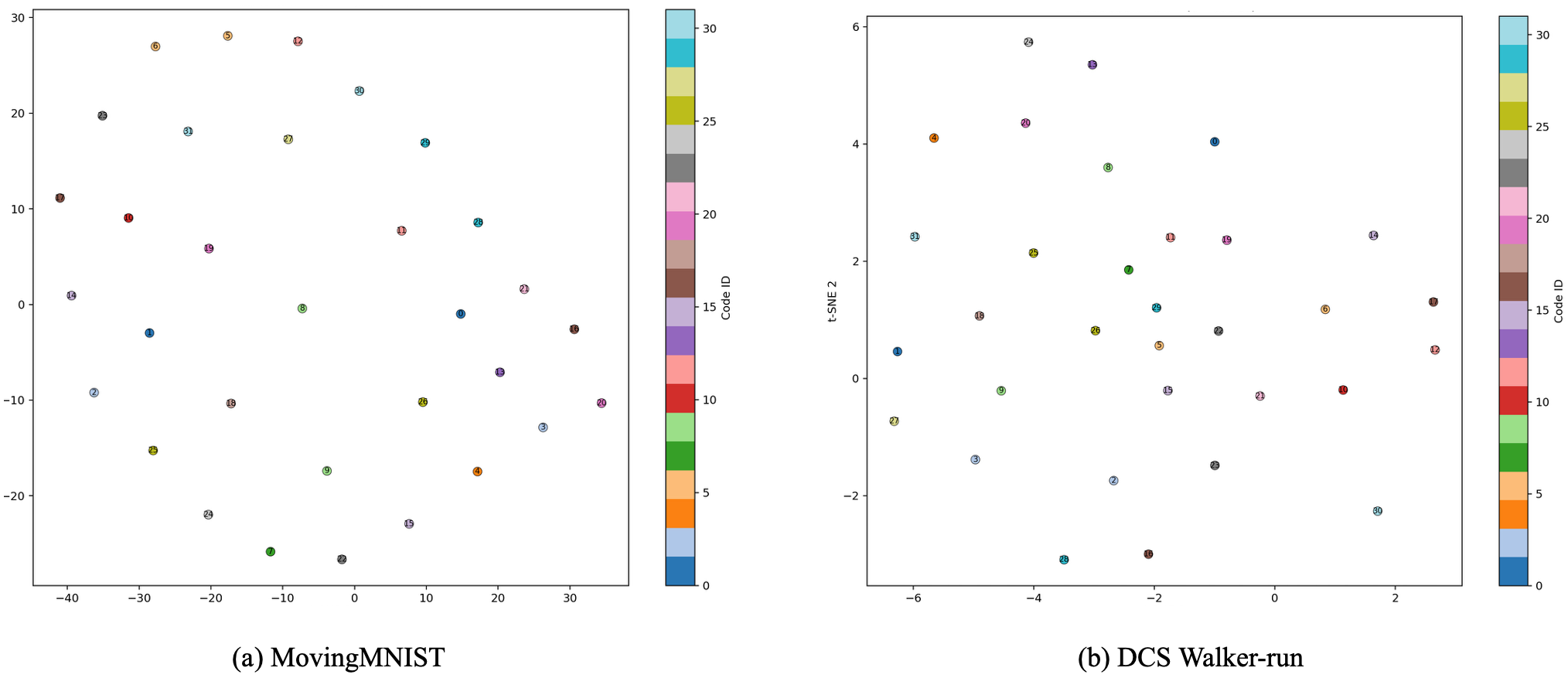
We provide additional qualitative visualizations of the learned observed-transition vocabulary. This visualization provides a qualitative view of how the discrete observed-transition primitives are organized in the learned vocabulary.

Code Assignment.

Fig. A2 shows example assignments on individual walker-run transitions. Similarly, Fig. A3 shows example assignments on individual Moving MNIST samples. For each sample, we visualize the current frame, the motion-centered input, the t-SNE (van der Maaten and Hinton 2008) projection of patch embeddings, and the corresponding assigned codebook entries on the patch grid or assigned observed-transition primitives on the patch grid. These examples illustrate how local transition patterns are mapped to discrete codebook primitives across different spatial regions.

More visualization from Zero-shot Transferability

Figure A4 shows extra visualizations for both MovingMNIST and DCS zero-shot transfer experiments.

Appendix E E. Baselines

E.1 LAPO (Schmidt and Jiang 2024)

LAPO is a monolithic latent action model that learns action-like representations from observation-only trajectories. Its inverse dynamics model (IDM) infers a latent action from consecutive observations, while its forward dynamics model (FDM) reconstructs or predicts the subsequent observation conditioned on the current observation and the inferred latent action. The entire scene transition is represented using a single latent action, providing a standard monolithic baseline for comparison with our localized and factorized representation.

Training Details

We train LAPO for $20$ k optimization steps following the experimental configuration used by LAOM (Nikulin et al. 2025). We evaluate latent action dimensions of $128$ and $256$ . Unless otherwise specified, the remaining settings follow the implementation from LAOM (Nikulin et al. 2025).

E.2 FLAM (Wang et al. 2025)

FLAM extends monolithic latent action models by decomposing a scene into multiple independent factors. Each factor infers its own latent action and predicts its own next-step factor representation, allowing the model to capture transitions involving multiple independently changing entities. In contrast to a single global latent action, this factorized formulation is designed to model complex multi-entity dynamics through a collection of factor-specific latent actions. We have additional discussion comparing object centric methods and motion centric methods (ours) in Appendix H.

Training Details

We follow the authors’ implementation. We use $d_{\mathrm{model}}=256$ , two transformer blocks, and $128$ latent $z$ channels. We evaluate models with $4$ and $8$ factors, referred to as slots in the implementation. Each factor uses an action codebook containing $16$ codes, and the VAE–VQ KL weight is annealed from $0$ to $2\times 10^{-4}$ . We use a sub-trajectory length of $10$ , a history length of $1$ , and $5$ prediction steps. The tokenizer consists of an IMPALA encoder, a LAPO decoder, and an FSQ quantizer. We use an input image size of $64$ , an FSQ codebook size of $1024$ , levels $(4,4,4,4,4)$ , $128$ latent channels, and a codebook dimension of $128$ . We train FLAM for $10$ epochs with batch size $32$ , learning rate $10^{-4}$ , zero weight decay, and gradient-norm clipping at $1.0$ . We additionally use xFormers attention, frame skip $1$ , HDF5 datasets, and random seed $42$ .

E.3 HiLAM (Kim et al. 2026)

HiLAM learns temporally extended latent skills on top of a pretrained low-level latent action model. The pretrained model first extracts a sequence of low-level latent actions from observation transitions, after which HiLAM aggregates their temporal patterns into higher-level latent skills. This hierarchical construction is intended to capture longer-horizon structure that may not be represented by latent actions learned from individual short-horizon transitions.

Training Details

We follow the default configuration provided in the authors’ implementation. We train HiLAM for $50$ k optimization steps with a learning rate of $10^{-4}$ and a latent action dimension of $64$ .

E.4 Motion LAPO (M-LAPO)

Motion LAPO augments LAPO with explicit motion inputs alongside the pixel observations. It retains LAPO’s monolithic latent action formulation while exposing the model directly to motion information. This baseline therefore isolates the effect of explicit motion processing from the effects of localized encoding and patchwise quantization introduced by OTF-LAM.

Training Details

We train M-LAPO for $20$ k optimization steps with a latent action dimension of $128$ . All other settings follow those used for LAPO.

E.5 Factorized LAPO (F-LAPO)

Factorized LAPO replaces LAPO’s global latent action encoder and quantization mechanism with an OTF-LAM-style patch encoder and patchwise quantization. Unlike OTF-LAM, however, it does not use explicit motion inputs. This baseline isolates the effect of learning spatially localized discrete latent representations while retaining the remaining LAPO training framework.

Training Details

We train F-LAPO for $20$ k optimization steps with a latent action dimension of $128$ . All other settings follow those used for LAPO.

Appendix F F. Training Details

F.1 OTF-LAM-Pixel amd OTF-LAM-DINO

We train separate models for each environment and codebook size $K\in\{16,32,64,128\}$ . All models are trained for $20$ k optimization steps with batch size $512$ using AdamW (learning rate $10^{-4}$ , weight decay $0$ ) and gradient norm clipping of $1.0$ . The pretrained motion encoder and codebook are frozen throughout training.

F.2 Downstream Evaluation

We evaluate all pretrained latent action models using a two-stage downstream pipeline consisting of behavior cloning followed by supervised action decoding.

Behavior Cloning

The behavior-cloning policy receives a stack of three RGB frames and predicts the latent action inferred by the frozen latent action model. We use the first $1{,}000$ trajectories of each environment, batch size $512$ , AdamW with learning rate $10^{-4}$ and zero weight decay, and random seeds $\{0,1,2\}$ . OTF-LAM-Pixel policies are trained for $10$ epochs, while OTF-LAM-DINO policies are trained for $5$ epochs.

Action Decoding

The action decoder maps the predicted latent action together with the policy state representation to the environment action. We evaluate supervision budgets of $\{16,32,64,128\}$ trajectories, where we use $\{2.5$ k, $5$ k, $10$ k, $20$ k $\}$ optimization steps for each. All decoders are trained with batch size $512$ using AdamW with learning rate $3\times 10^{-4}$ and weight decay $0$ . Each trained policy is evaluated for $10$ episodes. We also train for three seeds, matching with behavior cloning.

Appendix G G. Additional Results

G.1 Full Results

Table A1: Mean and standard deviation of average return across 10 trajectories over 3 random seeds.

Model	Cheetah-Run		Walker-Run
Model	Mean return	Std.	Mean return	Std.
LAPO-128 (Schmidt and Jiang 2024)	11.48	7.19	28.71	7.59
LAPO-256 (Schmidt and Jiang 2024)	13.55	5.40	23.91	2.82
M-LAPO	9.68	4.18	23.93	4.40
F-LAPO	11.56	3.39	23.44	5.79
FLAM-4 (Wang et al. 2025)	40.52	27.82	28.44	6.25
FLAM-8 (Wang et al. 2025)	26.29	16.90	29.65	7.28
LAPO-128 (Schmidt and Jiang 2024)	11.48	7.19	28.71	7.59
OTF-LAM-Pixel (best config.)	20.48	19.74	27.45	7.54
OTF-LAM-DINO (best config.)	43.80	26.98	28.87	8.23

Table A2: Effect of supervision amount on downstream performance.

Model	codebook size	supervised trajectories	Cheetah-Run		Walker-Run
Model	codebook size	supervised trajectories	Mean return	Std.	Mean return	Std.
OTF-LAM-DINO	16	16	34.06 (–)	19.12	27.68 (–)	6.03
		32	41.61 ( $\uparrow$ 7.55)	22.91	28.74 ( $\uparrow$ 1.06)	7.00
		64	55.69 ( $\uparrow$ 21.63)	30.49	32.56 ( $\uparrow$ 4.88)	11.47
		128	60.71 ( $\uparrow$ 26.65)	30.72	33.91 ( $\uparrow$ 6.23)	11.66
	32	16	35.51 (–)	27.73	24.00 (–)	6.17
		32	37.75 ( $\uparrow$ 2.24)	22.16	28.08 ( $\uparrow$ 4.08)	6.67
		64	40.68 ( $\uparrow$ 5.17)	24.50	30.99 ( $\uparrow$ 6.99)	8.53
		128	50.96 ( $\uparrow$ 15.45)	28.71	38.30 ( $\uparrow$ 14.30)	15.30
	64	16	32.31 (–)	22.69	26.73 (–)	5.70
		32	36.10 ( $\uparrow$ 3.79)	21.75	28.36 ( $\uparrow$ 1.63)	7.87
		64	42.79 ( $\uparrow$ 10.48)	27.81	33.14 ( $\uparrow$ 6.41)	11.32
		128	46.39 ( $\uparrow$ 14.08)	31.92	38.97 ( $\uparrow$ 12.24)	12.88
	128	16	37.87 (–)	22.95	24.98 (–)	4.88
		32	40.02 ( $\uparrow$ 2.15)	24.04	29.04 ( $\uparrow$ 4.06)	8.40
		64	46.24 ( $\uparrow$ 8.37)	26.94	30.70 ( $\uparrow$ 5.72)	8.70
		128	46.88 ( $\uparrow$ 9.01)	33.27	38.54 ( $\uparrow$ 13.56)	13.74
LAPO-256	-	16	4.80 (–)	1.96	26.20 (–)	2.40
		32	13.55 ( $\uparrow$ 8.75)	5.40	23.91 ( $\downarrow$ 2.29)	2.82
		64	12.62 ( $\uparrow$ 7.82)	5.41	25.59 ( $\downarrow$ 0.61)	5.31
		128	14.74 ( $\uparrow$ 9.94)	7.32	25.10 ( $\downarrow$ 1.10)	4.48

Table A3: Downstream evaluation of OTF-LAM and OTF-LAM-DINO with different motion vocabulary sizes. Std. is computed as root mean square across three random seeds.

	K	OTF-LAM		OTF-LAM-DINO
	K	Mean return	Std.	Mean return	Std.
Cheetah-Run	16	12.24	9.79	40.85	23.69
	32	17.06	14.66	43.80	26.98
	64	16.70	18.30	33.09	20.46
	128	20.48	19.74	42.92	26.01
Walker-Run	16	26.52	5.53	28.87	8.23
	32	25.62	4.67	27.64	6.57
	64	24.66	5.02	28.70	7.74
	128	27.45	7.54	27.65	8.09

We provide the complete quantitative results, including the full baseline comparison (Table A1), the effect of supervision amount (Table A2), and the codebook-size ablation for OTF-LAM and OTF-LAM-DINO (Table A3).

G.2 Effect of Supervision Amount

Table A2 examines the effect of increasing the amount of supervised trajectories used for downstream policy learning. For a controlled comparison, OTF-LAM-DINO and LAPO-256 use the same latent action dimension. Across all codebook sizes, OTF-LAM-DINO consistently benefits from additional supervision. Performance improves almost monotonically as the number of labeled demonstrations increases, with the largest gains typically occurring between the lowest and highest supervision budgets. On Cheetah-Run, the average return often improves by roughly $10$ – $30$ points depending on the codebook size, while Walker-Run exhibits similarly consistent, although generally smaller, improvements.

The benefit of additional supervision is particularly pronounced when using larger codebooks. Models with larger motion vocabularies generally start from stronger representations under limited supervision and continue to improve as more labeled data becomes available. In contrast, smaller codebooks remain competitive in the low-supervision regime but tend to saturate earlier. For comparison, LAPO-256 shows substantially weaker scaling with supervision. While increasing the number of demonstrations improves performance on Cheetah-Run, the gains are considerably smaller than those of OTF-LAM-DINO. On Walker-Run, additional supervision provides little benefit and occasionally leads to slight performance degradation, suggesting that its learned latent actions are less amenable to downstream policy learning. Overall, these results indicate that the representations learned by OTF-LAM-DINO remain informative across a wide range of supervision budgets, allowing downstream policies to effectively exploit additional labeled demonstrations, whereas conventional monolithic latent actions exhibit much weaker scalability with supervision.

G.3 Effect of Motion Vocabulary Size

We study how the size of the motion primitives affects downstream policy performance. Table A3 reports evaluation returns for OTF-LAM and OTF-LAM-Dino with different codebook sizes $K$ on cheetah-run and walker-run, averaged over $3$ seeds, where each seed evaluates $10$ trajectories. For decoder-based OTF-LAM, cheetah-run performance improves consistently as $K$ increases. This suggests that a larger vocabulary provides a more expressive set of transition primitives for this environment. On walker-run, however, performance is relatively stable across codebook sizes, with all variants achieving similar returns, indicating that the required transition structure in walker-run is captured even by smaller vocabularies, or that downstream control is less sensitive to additional motion primitives in this setting. OTF-LAM-DINO shows a different pattern. It improves over decoder-based OTF-LAM for every tested $K$ in both environments, suggesting that prediction in a frozen DINO representation space provides a useful downstream interface for the learned latent actions. However, its performance is not monotonic in $K$ . Overall, codebook size should be viewed as an environment- and architecture-dependent capacity parameter rather than a monotonic source of improvement. A more systematic study of how vocabulary size interacts with motion complexity, representation-space prediction, and downstream control remains future work.

Appendix H H. Discussion

Toward a General-Purpose Motion Tokenizer

A promising direction for future work is to scale OTF pretraining across heterogeneous video datasets. Similar to large-scale optical-flow training, one could combine trajectories from different environments, embodiments, and visual domains to learn a shared motion tokenizer rather than training a separate tokenizer for each environment. Such a tokenizer could provide a general vocabulary of local transition patterns that transfers across tasks and serves as a foundation for downstream latent action learning. Developing this type of broadly pretrained motion tokenizer will require addressing differences in appearance, temporal scale, camera motion, and embodiment across data sources.

Relation to Object-Centric Learning

OTF-LAM does not require an explicit decomposition of a scene into semantic objects. Object-centric methods based on learned slots can be sensitive to initialization, architectural choices, and the number of slots, and their decompositions may become unreliable in visually complex scenes. In contrast, OTF-LAM quantizes localized transition evidence directly and composes the resulting primitives without requiring stable object assignments. The learned primitives need not correspond one-to-one with objects, but they provide a simpler and potentially more robust basis for representing local dynamics.