Not-quite-human tastes: the stylized omnivorousness of LLM survey surrogates.
Abstract.
Large-language models have proven to be remarkable if inconsistent parrots of public attitudes and opinions. The extent to which LLMs are able to produce reasonable approximations of cultural taste remains an open empirical question that becomes more urgent by the day, with market research companies already offering provisional ‘synthetic’ survey panels and the contamination of standard survey data from LLM-generated responses. In this study, we build on past work on silicon sampling by extending considerations of its algorithmic fidelity and alignment to the domain of cultural consumption. We use large-language models from OpenAI, Anthropic, and DeepSeek to each produce 277,470 () silicon surrogates of survey respondents from the Survey of Public Participation in the Arts (SPPA). We find these silicon surrogates’ tastes to be highly stylized facsimiles of human tastes. (1) Silicon samples have a systematic postive-bias for liking, resulting in inflated ecological estimates of tastes. The individual-level bias of silicon samples are not well-explained by the WEIRD-bias often discussed in the literature. (2) The complex relationality in real taste structures is completely lost among silicon samples. (3) Finally, very little of the known cultural alignment between tastes and social space are preserved. Silicon samples attenuate age-taste associations, resurrect anachronistic class-taste associations, caricaturize gender- and race-taste associations.
Key words: AI, taste, consumption, culture, silicon sampling, meta-analysis.
1. Introduction
Large-language models have proven to be remarkable if inconsistent chameleons of public attitudes and opinions (e.g Argyle et al. 2023; Bisbee et al. 2024; Santurkar et al. 2023; Kozlowski et al. 2024). The extent to which LLMs are able to produce accurate surrogates of cultural taste and consumption remains an open empirical question that becomes more urgent by the day, with market research companies already offering provisional “synthetic” survey panels (e.g. Currie 2025; VeraSight 2026). In this study, we build on past work on silicon sampling by extending considerations of its algorithmic fidelity and alignment to the domain of cultural tastes. We use large-language models from OpenAI, Anthropic, and DeepSeek to produce silicon surrogates of respondents from the Survey of Public Participation in the Arts (SPPA), compare the tastes and preferences from these silicon samples against their SPPA counterparts. First, we evaluate the ecological and relationality fidelity of these silicon tastes. Then, using a mixed-effects meta-analysis framework, we evaluate the multivariate associations of silicon tastes with key dimensions of social space.
We find the following. (1) Silicon samples have a systematic postive-bias for liking, resulting in inflated ecological estimates of tastes. The individual-level bias of silicon samples are not well-explained by the WEIRD-bias often discussed in the literature. (2) The complex relationality in real taste structures is completely lost among silicon samples. (3) Finally, very little of the known cultural alignment between tastes and social space are preserved. Silicon samples attenuate age-taste associations, resurrect anachronistic class-taste associations, caricaturize gender- and race-taste associations.
Assessing the fidelity of such silicon tastes is crucial for two main reasons. First, silicon tastes, if faithful, allow for research designs formerly infeasible. Silicon sampling make a seductive promise to researchers. LLMs answer surveys quickly, cheaply, and without fatigue or complaint. It may now be possible to cheaply and quickly produce surveys of public opinion; to field surveys that were thought to be too long, laborious, or boring; to effectively go back in time and ask and then re-ask the questions that you couldn’t or didn’t think so. For social scientists interested in the study of tastes, silicon samples could facilitate finer-grain investigations than previously possible. Present surveys of cultural taste tend to rely on responses to fuzzy cultural categories, such as genres. As Vandebroeck (Vandebroeck 2022) points out, this convention assumes (a) that consumers possess a taxonomy of cultural categories that’s more or less similar to the one posited by the survey and (b) that the cultural categories themselves are not the subject of significant contestation and ambiguity. Genres, in other words, are inherently fuzzy, and it is far from obvious that respondents share the taxonomy a survey imposes on them. Yet fielding surveys that probe finer aspects of cultural taste is difficult, since this makes a survey long, tedious, and expensive. Were silicon samples to prove faithful, they would let researchers interrogate taste at the level of specific works, performances, or sub-genres, and to vary the framing of cultural categories experimentally, at a scale and cost that fielding such instruments on human respondents could never match. Further, silicon samples would facilitate interpolated projections of cultural taste in time and space, allowing up to improve our understanding of the ecology of tastes over time. Extrapolation of public opinion surveys into social space with limited support is a dangerous proposition, but interpolation over known spaces may be plausible and rewarding in and of itself. There are no notable panel studies of cultural taste, and few repeated cross-sectional studies of cultural taste (Ma 2020). Silicon sampling may allow for the construction of such data-sets and produce generative preliminary analysis of changes in taste ecologies over time.
Second, silicon sampling of public opinion and behavior is quickly expanding. While the social scientific community has urged caution when it comes to use of silicon samples (e.g. Gao et al. 2025; Bisbee et al. 2024; Broska et al. 2025), these norms are unsettled and frequently transgressed. It’s important to have a better understanding of the quality, biases and limitations of silicon samples across a breadth of sociologically relevant domains (Lyman et al. 2025). Assessing the fidelity of silicon sampling is pressing because the practice is expanding rapidly—in the range of domains to which it is applied, in the sophistication of its methods, and in its rapid expansion by survey and market research companies. Researchers have used LLMs to simulate responses to contentious political items drawn from the American National Election Studies (Li et al. 2024), German public opinions (Ma et al. 2025), and public opinions about climate change (Lee et al. 2024), to project audience attitudes and policy preferences, and to model public-health attitudes such as vaccine acceptance. Importantly, a robust commercial interest in the provision of silicon samples has emerged. Survey and market research companies like Qualtrics and VeraSight have already begun experimental rollouts of “synthetic panels” that are built using silicon samples (Isaza 2024; Currie 2025; VeraSight 2026). Ordinary survey respondents also frequently turn to LLMs and chatbots to generate ostensibly ‘human’ response surveys, meaning that even researchers who use orthodox survey methods are likely to face non-negligible contamination of ‘synthetic’ responses in their data (Zhang et al. 2025; Veselovsky et al. 2025). The techniques themselves behind silicon sampling have also grown more elaborate. Beyond zero-shot prompting, some scholars now fine-tune models on structured survey data to better recover response distributions, attach parameter-efficient persona adapters trained on large persona banks, and query models directly for entire response distributions rather than aggregating individual answers. The ambition of these efforts is captured by the emergence of large reference datasets purpose-built for constructing “digital twins” of individual respondents. Others have used low-ranked adaptations of large foundation models to finetune and produce locally-hosted silicon samples (Dash et al. 2025). The faster silicon sampling diffuses across these settings, the more consequential its hidden biases become, and the more urgent it is to establish where it is, and is not, faithful.
2. Literature review
2.1. Silicon sampling and the study of taste
Large language models (LLMs) are probabilistic machine learning models that are used to process and produce textual data. At a high level, LLMs resemble the autocomplete technologies that have become on search engines and other digital spaces, but with considerably greater scale and sophistication (Bail 2024). They power the dialogue agents that have already experienced widespread consumer adoption. In this study, we extend ongoing work that applies LLMs to survey research. In particular, we focus on the use of LLMs to simulate synthetic human samples in public opinion surveys, a practice often referred to as silicon sampling.
The intuition behind silicon sampling is simple. Homo silicus has advanced to such a state that many LLMs are able to converse and reason like humans, that the prospect of AI passing Turing tests just about seems a fait accompli (Dillion et al. 2023). If homo silicus really was capable of providing such a great facsimile of human responses, then it may be possible to productively sample responses from LLMs, the same way we would from human populations. LLMs by the nature of their training and design are computational models of humans and likely possess a great deal of latent social information (Horton 2023). This latent information can often evince itself negatively in different guises of algorithmic bias, Argyle et al. ((2023)) argue that it may be possible to instead think of them in productive terms as a model of the “complex reflection of the many various patterns of association between ideas, attitudes, and contexts present among humans.” The algorithmic fidelity of LLMs, when appropriately conditioned, means that researchers may be able to induce the model to produce outputs that correlate with the attitudes, opinions, and experiences of distinct human subpopulations. As George Box put it, while all simplified models of human behavior are necessarily wrong, some are useful. So it may be the case for silicon samples of human respondents. Work is also underway exploring the applications of synthetic surrogates of human respondents in domains beyond survey research, from agent-based modeling, to psychological experiments, to behavioral economics experiments, to market research (Chen et al. 2023; Dillion et al. 2023; Horton 2023; Park et al. 2023; Goli and Singh 2024).
In our study, we advance ongoing work on the robustness and bounds of silicon sampling by applying to cultural fields, in particular exploring the application of silicon sampling to the case of public opinion surveys of cultural taste. Taste in its most literal form refers to gustatory taste, our perception of sweet, salty, bitter, sour, and savory sensations as mediated by a physiologically-defined chemosensory system. From the 16th century and on, however, taste acquired a separate metaphorical meaning as an expression of a person’s aesthetic orientation towards culture, that is, cultural taste. Cultural taste is commonly operationalized as a person’s first-order preferences, feelings, or desires towards an object in a cultural field (Ma 2024). We use the term “silicon tastes” to refer to the tastes and preferences expressed by silicon surrogates of human respondents.
2.2. Assessing the fidelity of silicon tastes
How faithful are silicon tastes to their carbon counterparts? We contribute to ongoing work examing the bounds and robustness of silicon sampling by examing the quality and fidelity of synthetic cultural tastes. We assess (1) the ecological fidelity of silicon tastes, and whether such validity is mediated by the so-called WEIRD bias of LLMs, (2) the higher-order relations among silicon tastes, and (3) the fidelity of taste-to-social-space associations inferred from silicon samples. We ask three main research questions.
-
(1)
How faithful are the ecological estimates of cultural tastes produced by silicon samples? And to what extent are discrepancies in estimates explained by the WEIRD-bias?
-
(2)
To what extent do silicon samples preserve the relationality among tastes?
-
(3)
To what extent are known cultural associations between tastes and social space preserved among silicon samples?
To answer the first question, we compare the ecological estimates of cultural tastes for 17 genres of music from real and silicon samples. Then, we compute and model the Jaccard distance between the real and silicon tastes. To answer the second, we examine and compare the correlation matrices of real and silicon tastes. To answer the third, we model the coefficient bias of silicon samples through a mixed-effects meta-regression.
2.2.1. On the ecological fidelity of silicon tastes.
Early work were quick to establish the surprising accuracy of silicon samples, especially when it came to ecological estimates. In their seminal paper, Argyle et al. 2023 first observed “a high degree of correspondence between reported two-party presidential vote choice proportions from GPT-3 and ANES respondents.” For instance, GPT-3 silicon respondents reported an aggregate 0.391 probability of voting for Mitt Romney for the 2012 US Presidential elections; the same percentage from the ANES was 0.404 (Argyle et al. 2023). Bisbee et al. similarly created synthetic surrogates to the ANES, and find “every synthetic mean falls within one standard deviation of the ANES average” (Bisbee et al. 2024, pg. 6). Studies of silicon samples in domains away from American public opinion of politics have also found success. Brand et al. ((2023)) use a silicon sampling approach to replicate conjoint studies of consumer preference. They report that “[o]verall, the resulting estimates are realistic, both in magnitudes and in distribution … a conjoint-like approach to preference estimation yields results that are strikingly similar to those found in a recent survey of real consumers conducted by Fong et al., as well as to additional human surveys we conduct.” Lee et al. 2024 find they are reasonably good at reproducing ecological estimates of American public opinions towards climate change. Dillion et al.’s ((2023)) likewise find that silicon samples of moral judgements to be surprisingly well-aligned with those of human participants. The extent to which the same might apply to silicon panels of cultural tastes remains an open empirical question.
Further, we ask if discrepancies in ecological fidelity of silicon tastes may be attributable to what we term WEIRD-alignment bias (e.g. Bulté and Rigouts Terryn 2025; Liu et al. 2024). There can be considerable between-group variance in algorithmic fidelity, with divergences from real data particularly high among groups from communities that are underrepresented in the training data sets of today’s foundation models (Madden 2025; Masoud et al. 2025). The unevenness of the training data may result in the systematic misalignment of cultural tastes across the board, such that they are much more faithful for Wealthy, Educated, Industrialized, Rich and Democratic (WEIRD) sub-populations than for others (Xiao et al. 2025; Santurkar et al. 2023). We ask if such WEIRD-alignment bias might also explain systematic divergences in the ecological fidelity of silicon tastes.
2.2.2. The relationality of silicon tastes.
The fidelity of silicon samples strike many as intuitively implausible; on closer examination, many researchers have uncovered many discrepancies between real survey samples and their silicon counterparts. A persistent finding across studies is that the fidelity of silicon samples are restricted to the coarsest of ecological estimates (e.g. Bisbee et al. 2024). Dig any deeper, and you see clearly the discrepancies and human data. For instance, researchers have noticed that silicon samples are uncannily precise in their estimates, underestimating the natural entropy to human responses (Bisbee et al. 2024; Li et al. 2024).111Silicon samples often exhibit extremely high homogeneity to their responses (Li et al. 2024). LLMs think like monoliths, “consistently overestimate how common the main opinion is within a subgroup” while erasing minority views (Li et al. 2024, pg. 28). Dominguez-Olmedo et al. also observe that “natural variations in entropy across questions are not reflected in models’ responses” (Dominguez-Olmedo et al. 2024). Silicon samples are poor at capturing the complex relationalities that exist among persons and non-person subjects in the social world (Bisbee et al. 2024). If this tendency persists among silicon tastes, then this represents a serious threat to the validity of silicon samples in the study of culture.
Tastes are fundamentally relational (Bourdieu 1984; Martin 2003; Emirbayer 1997). The social meaning of cultural objects, preferences, judgements, and tastes are developed in reference to one another; their relational properties lend them inherent meaning (Puetz 2021).222This also explains why geometric data analyses are so popular among certain subfields in the sociology of culture (e.g. Atkinson 2026) For example, the label of “middle-brow” that gets applied to certain cultural genres or objects is a relational label that requires the precedent construction of a high/low status bifurcation that is shared among a community – it is not an objective quality of said genre or object (Brown and Grover 2011; Lizardo and Skiles 2012; Seabrook 2000). For two persons to have similar tastes, it is not sufficient for them to coincide on one preference, but rather coincide on a broader set of preferences and versions (Goldberg 2011). For silicon tastes to be faithful, they must preserve not just ecological estimates of one variety of taste, but rather preserve the fidelity of the set entire. If taste (say, classic rock) goes with taste (say, blues) in the human data, then such covariations must also be observed in the silicon sample. The extent to which silicon samples preserve the relationality of tastes remains an open empirical question.
2.2.3. The fidelity of multivariate associations.
There are other higher-order attributes of silicon samples that often fall-short. Silicon samples often contain fundamentally different multivariate associations from real survey samples. Compare, for instance, the regression coefficients inferred from silicon samples. Bisbee et al. note that “[w]hen we regress feeling thermometer scores on respondents’ demographic attributes – the type of analysis common in public opinion research – the synthetic sample would frequently lead us to draw different inferences than if we relied on human respondents” (Bisbee et al. 2024, pg. 2). If this persists for cultural tastes, then, this may prove to be an enormous problem for usefulness of silicon samples in this domain. Taste is famously known to be socially located. In Distinction, Bourdieu ((1984)) famously uses the case of taste to illustrate the dialectical relationship between subjective agency and social structure. For this reason, tight taste-class homologies have been observed in a range of sociocultural contexts (e.g. Simmel 1957; Bourdieu 1984; Galbraith 1998; Accominotti et al. 2018; Atkinson 2016). Such multivariate associations between taste and social space are not limited to class alone, but also extend to other important organizing principles of social life, such as gender (Bourdieu 2001), race (Atkinson 2026), or life-stage (Ma 2020). We ask if the multivariate associations between tastes and social space observed among silicon tastes are faithful to those observed in human survey samples.
3. Data and methods
3.1. Data source
The SPPA is a repeated cross-sectional survey that measures cultural attitudes and participation in the United States. From 1982 to 2022, the SPPA included items that tapped individuals’ preferences for music genres, assessing respondents’ likes for a range of musical genres. Due to its longevity and representativeness, the SPPA serves as an effectively “canonical” data that that has provided the empirical basis for an enormous body of research into cultural tastes (e.g. Peterson and Kern 1996).
3.2. Generating silicon samples
We follow conventional approaches to silicon sampling to begin (e.g. Argyle et al. 2023; Bisbee et al. 2024). For a given survey , we use an LLM model to generate a data set of matching synthetic responses . After instructing the LLM model to adopt a persona defined by a set of respondent characteristics, we then ask it to answer the same set of prompts contained in . We choose respondent personas and cultural taste questions to match questions that human respondents were asked in , allowing us to gauge how accurately and precisely the synthetic LLM responses capture actual public opinion. We generate synthetic samples using three different large-language models: (1) GPT 4.0, (2) Claude 3.7 Sonnet, and (3) DeepSeek R1. For each of the models, we set temperature to be 1.0, and constrain the maximum output tokens to 2,500.
3.2.1. Prompt settings
We closely follow a style of prompting that has become dominant in political science, in particular when it comes to the simulation of synthetic attitudes towards political affairs and elections (e.g. Argyle et al. 2023; Bisbee et al. 2024). In short, we provide an LLM-powered conversational agent with a context, and then ask the agent to provide a response to a close-ended survey questionnaire, and to enclose the response in a .csv format.
Because LLM responses converge relatively quickly, we follow conventions and generate 30 synthetic responses for each real human respondent in the true survey (Bisbee et al. 2024), yielding a final data set of 277,470 () responses.
3.3. Key measures
3.3.1. Music tastes
We operationalize taste using a set of items from the SPPA. Respondents are asked to provide a binary yes/no response to the question, “Do you like to listen to {music genre}?” Seventeen music genres are admitted into consideration: (1) classical or chamber music, (2) opera, (3) Broadway musicals or show tunes, (4) jazz, (5) blues or rhythm and blues, (6) gospel or other religious music, (7) country music, (8) bluegrass, (9) folk music, (10) classic rock, (11) alternative or independent rock, (12) pop music, (13) rap or hip-hop, (14) electronic or dance music, (15) reggae, (16) Latin or salsa music, and (17) Asian, African, or Middle-Eastern music. We treat each affirmative response as an expression of taste for that genre. For each respondent , we collect these affirmative responses into a taste set , defined as the subset of the seventeen genres for which respondent reports a liking. This set-valued representation of taste serves as the basic unit for the distance measures introduced below, while the genre-level binary indicators serve as the outcomes in the linear probability models described in Section 4.3.
3.3.2. Genre popularity
A recurring question in this study is whether the fidelity of silicon samples depends on the popularity of the genre being simulated. We therefore classify each of the seventeen genres according to its popularity. To ground this classification in observed listening patterns rather than ad hoc judgement, we turn to the Billboard Hot 100, the music industry’s benchmark weekly ranking of the best-performing songs in the United States. We compiled every weekly Hot 100 chart spanning January 2005 through January 2012 and assigned each charting song a genre, which allows us to rank the seventeen SPPA genres by how frequently they appeared on the charts over this seven-year window.333Weekly chart entries were scraped programmatically, and each unique title/artist pair was matched to a primary genre through the iTunes catalog; the SPPA genres were then ordered by their total number of chart appearances. From this ranking we obtain a three-tier ordering of the genres—“very popular,” “popular,” and “not popular”—which we collapse into a binary indicator that takes a value of for genres ranked either very popular or popular, and otherwise. This yields eight popular genres (pop, hip-hop, country, alternative rock, electronic music, Asian/African/Middle-Eastern music, reggae, and blues) and nine non-popular genres (bluegrass, Broadway, classical, classic rock, folk, gospel, jazz, Latin, and opera). This binary indicator enters our analyses in two ways: it partitions the Jaccard distance measure into popular- and non-popular-genre variants (Section 3.3.3), and it serves as a moderator, and as the basis for an interaction with the synthetic-data label, in the meta-regression (Section 4.3).
3.3.3. Jaccard distance
We use a distance measure based on Jaccard similarity (“Jaccard distance”) to measure the differences between synthetic and sample tastes. Jaccard similarity is a statistical measure used to quantify how similar two sets are by comparing their intersection to their union. Let refer to the set of music genres respondent expresses likings for. Let refer to the set of music genres the synthetic counterpart of would express likings for. The Jaccard similarity () between and is given by
We define Jaccard distance () simply as .
3.3.4. Coefficient bias
We use coefficient bias to operationalize the relationship between cultural tastes and social location. We estimate the coefficient bias of silicon samples in two stages. First, for each survey wave we fit a linear probability model and extract the coefficients of interest. Second, we treat these wave-level coefficients as observations in a mixed-effects meta-regression, which lets us pool them while distinguishing sampling error from systematic between-wave variation. A mixed-effects model assumes that each observed estimate departs from an underlying mean for two reasons: sampling error, and genuine between-wave heterogeneity. The latter can arise from true differences across waves in populations, historical periods, study designs, analytical methods, or in our case, distinct data-generating procedures.
Let index the survey waves generated in the study.444The waves comprise the original SPPA data, 30 bootstrap samples of the 2011 SPPA wave, 30 waves from OpenAI, 30 from DeepSeek, and 15 from Anthropic. For each survey wave , we fit a separate linear probability model for each genre , where person ’s taste for genre is expressed as
where the independent variables include the terms for (a) age, (b) age2, (c) income (in US$1,000s), (d) gender (coded as a binary where 1 = woman), (e) race (coded as a binary where 1 = white), (f) years of education, and (g) urban residence (coded as a binary where 1 = urban). We are interested in four key estimands from each model: (1) the main effect of age, , (2) the main effect of gender, , (3) the main effect of income, , and (4) the main effect of race, .
We then fit a mixed-effects model to each estimand. Let be the observed estimate of the age estimand from survey wave , modeled as
Here denotes the value of the -th moderator variable for wave , while and represent the between-wave heterogeneity and the sampling error of each wave, respectively. We include the following moderator variables: (a) label for synthetic data, (b) label for popularity of music genre, (c) the interaction between synthetic data and popularity of genre, (d) a label for large magnitude effect and (e) the interaction between synthetic data and the large magnitude effect. The construction of these labels was discussed above. We fit the model using the restricted maximum-likelihood estimator, as implemented by the metafor package in R. We repeat the same procedure for , , and .
4. Results
4.1. Taste inflation
First, we assess the fidelity of ecological estimates produced from silicon samples. Table 1 reports ecological estimates of music tastes across the different survey samples. We find a pervasize positive bias across silicon samples from all LLM providers. That is to say, silicon surrogates over-like, are much more likely to express preferences (“likings”) for music genres than real persons. This tendency becomes particularly salient when considered in the aggregate. When looking at an additive index of music tastes555This is the standard measure of omnivorousness used in cultural sociology (e.g. Peterson and Kern 1996)., we can observe a clear failure in ecological estimates of taste: silicon respondents look like hyper-omnivores when compared to flesh-and-blood counterparts.
4.1.1. Pervasive positive bias (over-liking).
The deltas in Table 1 are overwhelmingly positive across all three providers. silicon respondents over-estimate the share of the population that likes a genre for 10 of the 17 genres under OpenAI, 14 under DeepSeek, and 13 under Anthropic. That is, silicon respondents say they “like” genres far more often than real respondents do. The positive deltas are also large in magnitude, reaching percentage points for folk music (OpenAI), for gospel (DeepSeek), and for gospel (Anthropic). By contrast, under-estimation is both rarer and milder: only three genres – ethnic music, reggae, and Latin music – are under-liked by every provider, and the largest under-estimate in the entire table is just percentage points (reggae, OpenAI).
4.1.2. Hyper-omnivorous, especially in nonpopular genres.
All of this aggregates into a peculiar variety of omnivorousness among silicon respondents. If contemporary American tastes are omnivorous (e.g. Peterson and Kern 1996), then silicon samples of the same may be described as hyper-omnivorous. On average, real SPPA respondents report liking of the seventeen genres; their silicon counterparts inflate this omnivorousness index by percentage points under OpenAI, under DeepSeek, and under Anthropic—a near-doubling of the apparent breadth of taste for the first two providers. The enormous disjuncture between the two provides the clearest failure of silicon sample fidelity. This hyper-omnivorous bias is magnified among the non-popular genres of music. Against a human baseline of , the mean share of non-popular genres liked rises by (OpenAI), (DeepSeek), and (Anthropic) percentage points; the corresponding inflation for popular genres is smaller, at , , and points against a baseline of .
| OpenAI | DeepSeek | Anthropic | |||||
| SPPA | Delta | p-val | Delta | p-val | Delta | p-val | |
| Popular Genres (% liked) | |||||||
| Pop music | 37.09 | 12.97 | 0.00 | 11.48 | 0.00 | 9.05 | 0 |
| Hip-hop | 19.02 | -0.66 | 0.25 | 0.32 | 0.58 | 5.22 | 0 |
| Country music | 43.62 | 33.56 | 0.00 | 30.10 | 0.00 | 32.94 | 0 |
| Alternative rock | 19.82 | -1.51 | 0.01 | 2.90 | 0.00 | 4.45 | 0 |
| Electronic music | 15.18 | -4.21 | 0.00 | 0.37 | 0.49 | 4.83 | 0 |
| Ethnic music | 8.47 | -0.63 | 0.12 | -3.74 | 0.00 | -3.42 | 0 |
| Reggae | 16.09 | -9.15 | 0.00 | -1.76 | 0.00 | -5.12 | 0 |
| Blues | 30.94 | 42.66 | 0.00 | 61.49 | 0.00 | 26.64 | 0 |
| Non-popular Genres (% liked) | |||||||
| Bluegrass | 18.64 | 52.15 | 0.00 | 45.68 | 0.00 | 41.63 | 0 |
| Broadway | 22.15 | 19.92 | 0.00 | 29.13 | 0.00 | 13.14 | 0 |
| Classical music | 28.21 | 28.25 | 0.00 | 26.07 | 0.00 | 19.26 | 0 |
| Classic rock | 51.26 | 44.86 | 0.00 | 43.83 | 0.00 | 47.61 | 0 |
| Folk music | 18.76 | 63.61 | 0.00 | 42.13 | 0.00 | 26.50 | 0 |
| Gospel | 26.45 | 60.00 | 0.00 | 62.16 | 0.00 | 49.42 | 0 |
| Jazz | 27.73 | 37.13 | 0.00 | 29.51 | 0.00 | 3.90 | 0 |
| Latin music | 17.83 | -5.44 | 0.00 | -7.46 | 0.00 | -6.53 | 0 |
| Opera | 9.83 | -4.38 | 0.00 | 1.14 | 0.01 | -4.56 | 0 |
| Aggregate Tastes | |||||||
| Mean % of popular genres liked | 23.78 | 9.13 | 0.00 | 12.64 | 0.00 | 9.33 | 0 |
| Mean % of nonpopular genres liked | 26.52 | 32.29 | 0.00 | 29.41 | 0.00 | 20.43 | 0 |
| Mean % of all genres liked | 24.18 | 21.71 | 0.00 | 21.96 | 0.00 | 15.59 | 0 |
4.1.3. Taste inflation not explained by the minority penalty.
The minority penalty does not effectively explain the systematic inflation we observed above. Table 2 reports the coefficient estimates from a linear model of the jaccard distance between silicon samples (pooled) and SPPA data. The minority penalty hypothesizes that groups whose perspectives and discourse are less represented in the training corpora of large language models – racial minorities, the less educated, and the less affluent – should be the hardest to simulate, and thus exhibit the largest Jaccard distances. But that is not what we observe. In the All-genre model of Table 2, where a positive coefficient denotes greater distance and therefore worse fidelity, three of the four conventional status axes run in the opposite direction. We find that (a) wealthier respondents are more difficult to simulate, with each additional $1,000 of income raising the Jaccard distance by (); (b) white respondents are simulated worse, not better, than non-white respondents (, ); and (c) respondents with more education are likewise simulated worse, by per additional year of schooling (). Gender is the only axis on which the penalty holds: women are simulated worse than men (, ).
| Jaccard distance | |||
| All genres | Only popular genres | Only nonpopular genres | |
| Age | 0.02∗∗∗ | 0.04∗∗∗ | 0.003 |
| (0.03, 0.02) | (0.04, 0.03) | (0.003, 0.01) | |
| Age-squared | 0.002∗∗∗ | 0.0002 | 0.003∗∗∗ |
| (0.002, 0.003) | (0.0004, 0.001) | (0.002, 0.004) | |
| Income (1,000s) | 0.002∗∗∗ | 0.001∗∗∗ | 0.003∗∗∗ |
| (0.002, 0.003) | (0.001, 0.001) | (0.003, 0.004) | |
| Education (years) | 0.01∗∗∗ | 0.003∗∗∗ | 0.01∗∗∗ |
| (0.01, 0.01) | (0.003, 0.004) | (0.01, 0.01) | |
| Gender (woman) | 0.03∗∗∗ | 0.01∗∗∗ | 0.05∗∗∗ |
| (0.03, 0.03) | (0.003, 0.01) | (0.05, 0.06) | |
| Race (white) | 0.02∗∗∗ | 0.06∗∗∗ | 0.09∗∗∗ |
| (0.01, 0.02) | (0.07, 0.06) | (0.08, 0.10) | |
| Urban residence | 0.01∗∗∗ | 0.07∗∗∗ | 0.04∗∗∗ |
| (0.004, 0.01) | (0.07, 0.08) | (0.04, 0.03) | |
| Constant | 0.26∗∗∗ | 0.47∗∗∗ | 0.07∗∗∗ |
| (0.25, 0.28) | (0.45, 0.48) | (0.06, 0.09) | |
| Observations | 27,747 | 27,747 | 27,747 |
| R2 | 0.06 | 0.21 | 0.20 |
| Adjusted R2 | 0.06 | 0.21 | 0.20 |
| Note: | ∗p0.1; ∗∗p0.05; ∗∗∗p0.01 | ||
4.2. Relationality of tastes
Second, we investigate the relationality of silicon tastes by looking at the covariation matrices of tastes. Human tastes have a rich and persistent relational structure; in this regard, silicon tastes share little in common. As explained above, for each sample, we create a covariation matrix, where each cell contains the Cramer’s V association, , between a taste and taste . For clarity’s sake, we’ll refer to the Cramer’s V estimates coming from the SPPA as , and Cramer’s V estimates from the silicon and bootstrap samples as .
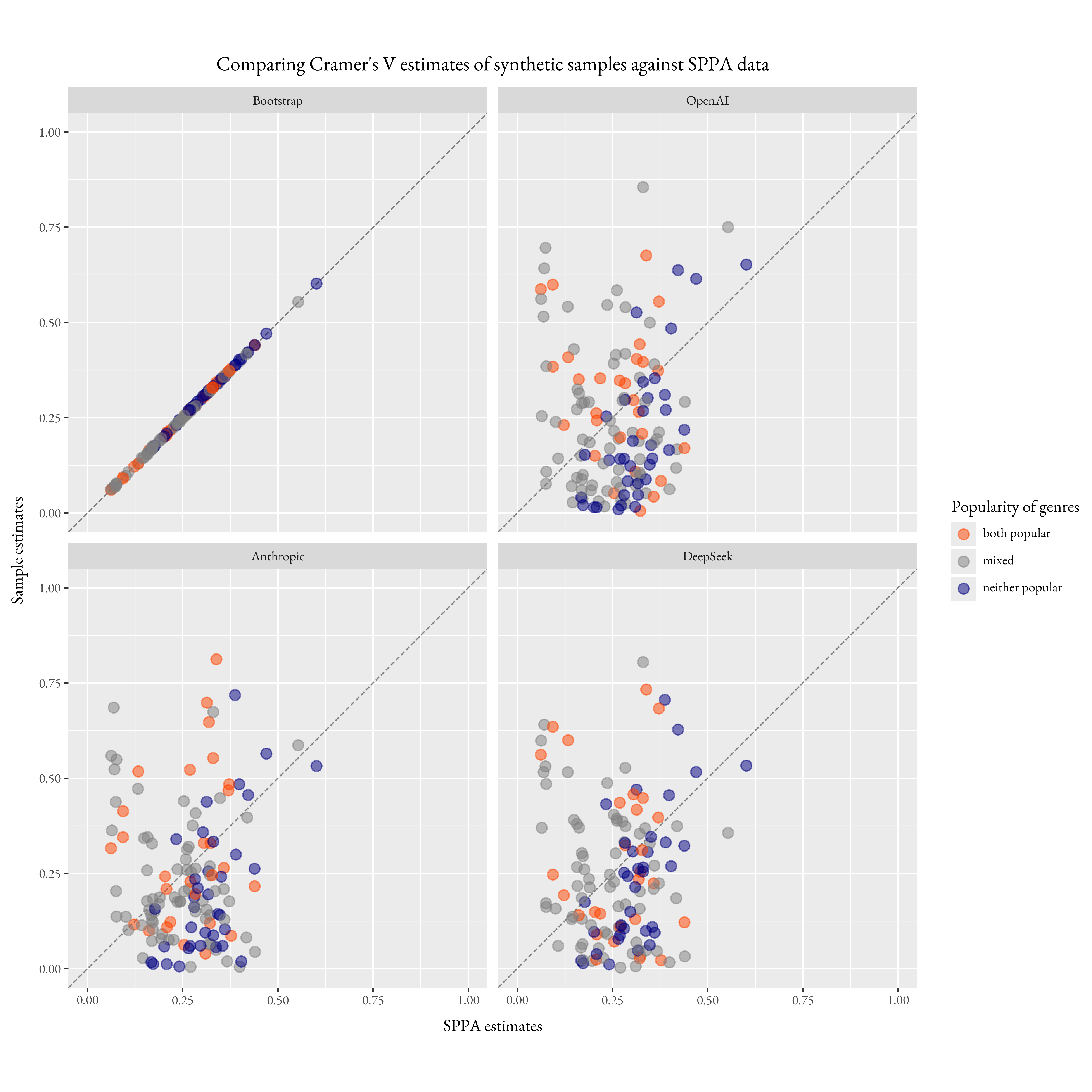
To compare the relationality of silicon samples and the SPPA survey, we first compare the Cramer’s V matrices obtained from each set. Figure 1 plot each genre pair’s sample Cramer’s V (, y-axis) against its Cramer’s V in the SPPA (, x-axis). A point falling on the dashed line denotes a pair whose association is reproduced exactly; points above the line are coupled more strongly in the sample than among human respondents, and points below it more weakly.666The bootstrap panel serves as a sanity check. Sample estimates from bootstrap samples lie almost perfectly along the diagonal across the full range of association strengths. Then, we take the delta between the Cramer’s V estimate obtained from the silicon sample and that obtained from the SPPA, . Figure 2 plots these comparisons as a grid of four heat maps, one for each sample source. Within each panel, the grid of cells corresponds to the pairs of music genres, and the color of a cell encodes the deviation between that sample’s Cramer’s V for the pair and the corresponding SPPA value; the diagonal, which would record a genre’s association with itself, is left blank. White cells indicate close agreement with the human data, warm (orange) cells mark genre pairs that the sample couples more strongly than human respondents do, and cool (blue) cells mark pairs it couples less strongly, with color intensity scaling with the size of the deviation.
Table 3 shows the covariance matrice with all silicon samples pooled together. Appendix A contains a more detailed breakdown of covariance matrices by each of the LLM providers.
4.2.1. The relational structure of silicon tastes is misaligned with human tastes.
Across all unique genre pairs (Table 3), the pairwise Cramer’s V values from the silicon samples are essentially uncorrelated with those from the SPPA (Pearson’s , Spearman’s ), whereas the bootstrap benchmark reproduces the human associations almost perfectly (). From Figure 1, we can also see obvious differences between the spread of the silicon samples and the true estimates. Cramer’s V estimates from silicon samples form a diffuse cloud bearing little relation to the diagonal. While bootstrap estimates are compressed into a narrow band (roughly to ), the silicon estimates fan out from near zero to above .
For a more substantive demonstration of such misalignment, consider first how silicon collapses the associations among the highbrow genres that are tightly bound in human taste. Comparing the SPPA matrix (Table 5) with the pooled silicon matrix (Table 3), several of the strongest human associations among these genres are sharply attenuated: the blues/classic rock association falls from to , blues/bluegrass from to , classical/opera from to , and Broadway/gospel from to . These pairs show up as cool (blue) cells in the LLM panels of Figure 2. In each case the silicon samples register an association close to zero where human respondents exhibit a substantial one, effectively dissolving the longstanding relations between these genres together.
Conversely, silicon manufactures associations among mainstream genres that humans do not actually link, visible as warm (orange) cells in Figure 2. The clearest cases pair a popular genre with an unpopular one. Relative to the SPPA, the silicon samples inflate the country/bluegrass association from to , electronic/hip-hop from to , hip-hop/bluegrass from to , folk/hip-hop from to , and electronic/gospel from to . Pairs such as hip-hop/bluegrass and electronic/gospel are all but orthogonal among real respondents, yet the silicon samples treat them as among the most tightly coupled tastes of all.
4.2.2. Silicon tastes have ersatz properties.
However, when looking at aggregate measures of relationality, silicon tastes can appear deceivingly similar to real tastes. The mean off-diagonal Cramer’s V—the average strength of association across all genre pairs—is for the pooled silicon samples (Table 3), only marginally below the observed in the SPPA (Table 5).777As a sanit check, the SPPA estimates are matched exactly by the bootstrap benchmark (; Table 9). At this coarsest level of analysis, silicon taste therefore looks about as “relational” as human taste. This apparent fidelity is precisely the trap: as Figure 1 and the near-zero correlations reported above make clear, the silicon samples recover the typical magnitude of association while almost entirely missing its structure—which pairs of genres actually hang together. Their relationality is in this sense ersatz, reproducing a summary statistic of human taste without the organization that gives it meaning.
4.2.3. Relationality fidelity is conditional on popularity; worse for less popular genres.
Relational fidelity is itself conditional on the popularity of the genres involved. The coloring of Figure 1 shows that the displacement from the diagonal is patterned by popularity: pairs in which both genres are popular (orange) sit disproportionately above the diagonal, pairs in which neither is popular (blue) fall below it, and mixed pairs (grey) scatter around it. Quantifying this pattern, the average deviation in Cramer’s V is for both-popular pairs, approximately zero for mixed pairs, and for neither-popular pairs. That is, silicon samples exaggerate the associatons between mainstream genres and attenuate the ones between less popular genres.
|
Pop music |
Hip-hop |
Country |
Alternative rock |
Electronic |
Ethnic music |
Reggae |
Blues |
Bluegrass |
Broadway |
Classical |
Classic rock |
Folk |
Gospel |
Jazz |
Latin |
Opera |
|
|---|---|---|---|---|---|---|---|---|---|---|---|---|---|---|---|---|---|
| Pop music | 0.45 | 0.30 | 0.40 | 0.41 | 0.17 | 0.24 | 0.14 | 0.41 | 0.12 | 0.20 | 0.13 | 0.34 | 0.30 | 0.21 | 0.21 | 0.17 | |
| Hip-hop | 0.45 | 0.54 | 0.35 | 0.72 | 0.24 | 0.57 | 0.18 | 0.61 | 0.13 | 0.31 | 0.29 | 0.59 | 0.45 | 0.13 | 0.25 | 0.13 | |
| Country | 0.30 | 0.54 | 0.19 | 0.51 | 0.36 | 0.48 | 0.19 | 0.80 | 0.09 | 0.05 | 0.29 | 0.47 | 0.46 | 0.30 | 0.19 | 0.11 | |
| Alternative rock | 0.40 | 0.35 | 0.19 | 0.48 | 0.06 | 0.07 | 0.15 | 0.22 | 0.06 | 0.08 | 0.05 | 0.11 | 0.56 | 0.09 | 0.05 | 0.11 | |
| Electronic | 0.41 | 0.72 | 0.51 | 0.48 | 0.24 | 0.34 | 0.17 | 0.52 | 0.06 | 0.18 | 0.27 | 0.40 | 0.57 | 0.12 | 0.22 | 0.10 | |
| Ethnic music | 0.17 | 0.24 | 0.36 | 0.06 | 0.24 | 0.26 | 0.10 | 0.35 | 0.03 | 0.10 | 0.25 | 0.25 | 0.19 | 0.16 | 0.11 | 0.07 | |
| Reggae | 0.24 | 0.57 | 0.48 | 0.07 | 0.34 | 0.26 | 0.17 | 0.44 | 0.10 | 0.19 | 0.27 | 0.43 | 0.09 | 0.21 | 0.20 | 0.08 | |
| Blues | 0.14 | 0.18 | 0.19 | 0.15 | 0.17 | 0.10 | 0.17 | 0.16 | 0.29 | 0.44 | 0.04 | 0.28 | 0.18 | 0.61 | 0.07 | 0.14 | |
| Bluegrass | 0.41 | 0.61 | 0.80 | 0.22 | 0.52 | 0.35 | 0.44 | 0.16 | 0.11 | 0.15 | 0.26 | 0.59 | 0.49 | 0.23 | 0.32 | 0.07 | |
| Broadway | 0.12 | 0.13 | 0.09 | 0.06 | 0.06 | 0.03 | 0.10 | 0.29 | 0.11 | 0.58 | 0.08 | 0.32 | 0.10 | 0.31 | 0.06 | 0.29 | |
| Classical | 0.20 | 0.31 | 0.05 | 0.08 | 0.18 | 0.10 | 0.19 | 0.44 | 0.15 | 0.58 | 0.11 | 0.51 | 0.09 | 0.59 | 0.18 | 0.26 | |
| Classic rock | 0.13 | 0.29 | 0.29 | 0.05 | 0.27 | 0.25 | 0.27 | 0.04 | 0.26 | 0.08 | 0.11 | 0.26 | 0.02 | 0.11 | 0.02 | 0.03 | |
| Folk | 0.34 | 0.59 | 0.47 | 0.11 | 0.40 | 0.25 | 0.43 | 0.28 | 0.59 | 0.32 | 0.51 | 0.26 | 0.28 | 0.24 | 0.29 | 0.15 | |
| Gospel | 0.30 | 0.45 | 0.46 | 0.56 | 0.57 | 0.19 | 0.09 | 0.18 | 0.49 | 0.10 | 0.09 | 0.02 | 0.28 | 0.11 | 0.16 | 0.05 | |
| Jazz | 0.21 | 0.13 | 0.30 | 0.09 | 0.12 | 0.16 | 0.21 | 0.61 | 0.23 | 0.31 | 0.59 | 0.11 | 0.24 | 0.11 | 0.09 | 0.26 | |
| Latin | 0.21 | 0.25 | 0.19 | 0.05 | 0.22 | 0.11 | 0.20 | 0.07 | 0.32 | 0.06 | 0.18 | 0.02 | 0.29 | 0.16 | 0.09 | 0.04 | |
| Opera | 0.17 | 0.13 | 0.11 | 0.11 | 0.10 | 0.07 | 0.08 | 0.14 | 0.07 | 0.29 | 0.26 | 0.03 | 0.15 | 0.05 | 0.26 | 0.04 |

4.3. Meta-regression
Finally, we consider how closely silicon samples are able to reproduce well-understood associations between tastes and social location. Table 4 contains results from our meta-regression models. We include original coefficient estimates from SPPA data, and the expected bias introduced by silicon samples. As mentioned above, we restrict ourselves to four variables: age, income, gender, and race. We discuss each in turn.
4.3.1. Synthetic samples associate music tastes with the young, with some exceptions.
In Table 4, the age-bias column is negative for 14 of the 17 genres, and significantly so () for 12 of them. The effect is to make the taste space look more youth-coded than it is among real respondents. Where the SPPA registers little or no age structure, silicon often manufactures a negative one, and where human data already show a youth tilt, silicon amplifies it. Alternative rock carries a modest true age effect of in the SPPA, yet picks up a bias of , roughly a twenty-fold inflation and the largest distortion in the table. Electronic music shows a similar pattern ( true, bias), as does pop music, where the human coefficient is effectively zero () but the silicon bias is . Hip-hop, already the most youth-coded genre in the human data (), is pushed further in the same direction ( bias). Classic rock presents the mirror image of this logic: among human respondents it is strongly elder-coded (), yet silicon still imposes a negative bias (), compressing one of the largest age gradients in the data rather than preserving it.
There are important exceptions to this general trend. The age/taste associations for country and bluegrass are faithfully reproduced by silicon samples. Country and bluegrass register age biases of essentially zero ( each, neither significant), suggesting that silicon reproduces their age/taste associations about as well as it reproduces any genre-level coefficient in the table. On the other hand, silicon samples exaggerate the senscence of a small set of music genres. Blues ( true, bias) and gospel ( true, bias) both pick up positive bias that pushes their age effects further into older territory—more than doubling the gospel gradient and adding substantially to blues.
4.3.2. Silicon samples resurrect retrograde class/taste homologies.
Net of education and the other covariates in our models, logged income barely structures musical taste in the SPPA. These null class/taste associations are consistent with broad changes in American taste structures over the past half-century away from a strict class-based hierarchy of taste. In Table 4, only four genres register statistically discernible income gradients among human respondents—pop (), Broadway (), classic rock (), and gospel ()—and all are small.888Logged income does not have any linear association with tastes for the canonical “high-brow” genres like classical (, ), opera (, ), jazz (, ), and blues (, ).
Silicon tastes, meanwhile, are retrograde. Silicon samples impose a class hierarchy on this near-blank field that is more redolent of the high-low brow taste hierarchy of the early-mid 20th century (e.g. Bourdieu 1984; Levine 1988). The income-bias column is positive for 11 of the 17 genres, and all 11 are statistically significant (), and its rank order tracks this retrograde t hierarchy almost textbook-perfectly. The largest fabricated gradients fall on “highbrow” genres: classical ( bias against a true effect of ), jazz ( against ), Broadway and blues (each against true effects of and ), folk ( against ), and opera ( bias, against true) completes the pattern among the highbrow genres. Jazz and blues are especially telling: among flesh-and-blood respondents they show no income gradient, yet silicon respondents treats them as affluent tastes.
4.3.3. Silicon samples caricaturize gender-taste associations
The SPPA data does contain real gender-taste associations, but they are modest and spread across several genres. Among silicon samples, only a smaller set of genres retain these gender-taste associations. Further, these associations are more exaggerated than they are in the SPPA sample – in this sense, gender-taste associations are effectively caricaturized. In Table 4, eight genres register significant gender (woman) coefficients in the SPPA: Broadway (), gospel (), pop (), country (), Latin (), classical (), blues (), and opera (). Hip-hop () and reggae () show small positive effects as well. Silicon samples caricaturize these gender-taste associations by concentrating them into a smaller set of genres. The three largest gender biases in the table fall on Broadway (), pop (), and classical (), each roughly three- to four-times the corresponding SPPA coefficient. Folk music also picks up a bias of against a true effect of essentially zero (), manufacturing a gender gradient where the SPPA had shown none. By contrast, silicon attenuates or reverses associations that complicate the stereotype. Country is the clearest case: women genuinely like country music more than men in the human data (), yet the silicon bias is negative (), erasing one of the strongest non-stereotypical gender effects in the table. Hip-hop and reggae show the same sign problem in miniature: both are slightly women-leaning in the SPPA ( each), but their biases run negative ( and ), pushing silicon samples toward a male-coded account of genres that human women in fact report liking at least as much as men.
4.3.4. Fictive race-taste associations.
Race-taste associations are where silicon samples show the poorest overall fidelity. In Table 4, the largest race (white) coefficients in the SPPA are country () and gospel (); no other genre exceeds (classic rock) or falls below (blues). Silicon samples push the implied coefficients far beyond this range, from for bluegrass () and for folk (), to for hip-hop (), producing an exaggerated racialization music taste that far exceeds anything in the SPPA data.
We can decompose this racialization into two distinctive components. First, silicon samples exaggerate mild biases for certain race-taste associations, such as folk ( on a true effect of ), bluegrass ( on ), and country ( on ). Broadway and classical music receive this on a smaller scale. In the SPPA, both genres are modestly white-leaning (Broadway ; classical ), yet silicon adds substantial positive race bias to each ( and ). Among genres that are registered as nonwhite-leaning in the SPPA, the amplification runs the other way: reggae ( on , roughly a nine-fold inflation and the most extreme entry in the table), jazz ( on ), hip-hop ( on ), and ethnic music ( on ). Second, silicon samples can also invent race-taste associations, sometimes ones that contradict the SPPA data. Electronic music is one example, where the race-taste coefficient is null under SPPA data, yet silicon samples assigns a bias of , fabricating a non-white association from nothing. Pop music is white-leaning in the SPPA (), but its race bias is , reversing the sign of the implied silicon coefficient to roughly . Latin music shows the same pattern in softer form ( true, bias). Opera’s modest white association () is cancelled entirely ( bias). Gospel is the strangest case: at , it carries one of the strongest Black-coded effects in the human data, yet silicon adds positive bias (), nearly erasing gospel’s racial signature—the lone instance in the table where a vivid racial association is attenuated rather than amplified.
| Age | Logged income | Gender (woman) | Race (white) | |||||||||||||
|---|---|---|---|---|---|---|---|---|---|---|---|---|---|---|---|---|
| Bias | Coef. est. | Bias | Coef. est. | Bias | Coef. est. | Bias | Coef. est. | |||||||||
| Est. | Est. | Est. | Est. | Est. | Est. | Est. | Est. | |||||||||
| Popular Genres | ||||||||||||||||
| Pop music | -0.183 | 0.01 | 0.001 | 0.94 | 0.016 | 0.01 | 0.030 | 0.01 | 0.328 | 0.01 | 0.083 | 0.01 | -0.240 | 0.01 | 0.075 | 0.01 |
| Hip-hop | -0.102 | 0.01 | -0.193 | 0.01 | -0.004 | 0.01 | -0.005 | 0.20 | -0.031 | 0.01 | 0.015 | 0.04 | -0.320 | 0.01 | -0.110 | 0.01 |
| Country | -0.001 | 0.70 | 0.062 | 0.01 | -0.007 | 0.01 | -0.003 | 0.64 | -0.046 | 0.01 | 0.054 | 0.01 | 0.229 | 0.01 | 0.202 | 0.01 |
| Alternative rock | -0.504 | 0.01 | -0.025 | 0.04 | 0.028 | 0.01 | 0.008 | 0.09 | -0.002 | 0.21 | -0.011 | 0.15 | 0.013 | 0.01 | 0.111 | 0.01 |
| Electronic | -0.279 | 0.01 | -0.067 | 0.01 | 0.014 | 0.01 | 0.000 | 0.95 | 0.000 | 0.99 | 0.010 | 0.16 | -0.152 | 0.01 | 0.016 | 0.12 |
| Ethnic music | -0.034 | 0.01 | 0.019 | 0.03 | 0.021 | 0.01 | -0.006 | 0.05 | 0.000 | 0.98 | -0.003 | 0.61 | -0.284 | 0.01 | -0.080 | 0.01 |
| Non-popular Genres | ||||||||||||||||
| Reggae | -0.038 | 0.01 | 0.044 | 0.01 | -0.001 | 0.58 | -0.001 | 0.83 | -0.036 | 0.01 | 0.015 | 0.04 | -0.365 | 0.01 | -0.039 | 0.01 |
| Blues | 0.150 | 0.01 | 0.121 | 0.01 | 0.067 | 0.01 | -0.004 | 0.49 | -0.005 | 0.58 | 0.023 | 0.02 | -0.069 | 0.01 | -0.117 | 0.01 |
| Bluegrass | -0.001 | 0.95 | 0.077 | 0.01 | 0.000 | 0.96 | -0.009 | 0.05 | -0.029 | 0.01 | -0.009 | 0.24 | 0.377 | 0.01 | 0.122 | 0.01 |
| Broadway | -0.036 | 0.01 | -0.015 | 0.24 | 0.067 | 0.01 | 0.015 | 0.01 | 0.453 | 0.01 | 0.107 | 0.01 | 0.096 | 0.01 | 0.059 | 0.01 |
| Classical | 0.016 | 0.01 | 0.018 | 0.20 | 0.096 | 0.01 | 0.006 | 0.20 | 0.125 | 0.01 | 0.032 | 0.01 | 0.058 | 0.01 | 0.061 | 0.01 |
| Classic rock | -0.119 | 0.01 | 0.201 | 0.01 | -0.005 | 0.01 | 0.016 | 0.01 | -0.014 | 0.01 | 0.003 | 0.74 | -0.043 | 0.01 | 0.183 | 0.01 |
| Folk | -0.014 | 0.01 | 0.061 | 0.01 | 0.027 | 0.01 | -0.007 | 0.09 | 0.082 | 0.01 | 0.003 | 0.72 | 0.384 | 0.01 | 0.099 | 0.01 |
| Gospel | 0.131 | 0.01 | 0.063 | 0.01 | -0.011 | 0.01 | -0.015 | 0.01 | -0.003 | 0.45 | 0.097 | 0.01 | 0.068 | 0.01 | -0.129 | 0.01 |
| Jazz | -0.051 | 0.01 | 0.098 | 0.01 | 0.078 | 0.01 | 0.007 | 0.19 | -0.015 | 0.44 | 0.006 | 0.52 | -0.331 | 0.01 | -0.072 | 0.01 |
| Latin | -0.032 | 0.01 | 0.047 | 0.01 | 0.003 | 0.01 | -0.003 | 0.50 | -0.015 | 0.01 | 0.039 | 0.01 | -0.023 | 0.01 | 0.063 | 0.01 |
| Opera | -0.070 | 0.01 | -0.008 | 0.37 | 0.025 | 0.01 | -0.004 | 0.28 | 0.011 | 0.01 | 0.023 | 0.01 | -0.025 | 0.01 | 0.024 | 0.01 |
5. Conclusion
Silicon sampling promises cheap, scalable substitutes for human survey respondents. This paper asks how far that promise extends to cultural taste—a domain where preferences are structured not only by aggregate levels of liking but by the relational organization of genres and their alignment with social location. Using 277,470 silicon surrogates from OpenAI, Anthropic, and DeepSeek, matched to respondents from the Survey of Public Participation in the Arts, we find that LLM-generated tastes are highly stylized facsimiles of human tastes: plausible at the surface, but systematically wrong in ways that would mislead researchers who reify them as interchangeable with flesh-and-blood data. In this study, we assessed the fidelity of silicon samples in three major ways, by considering (a) their ecological fidelity, (b) their relationality fidelity, and (c) how closely they are able to reproduce known multivariate associations between tastes and social location
At the ecological level, silicon samples over-like. Silicon respondents have a pervasive positive bias to their music tastes, so much so that they appear to be hyper-omnivores when compared to their SPPA counterparts. This is particularly so when it comes to less popular genres of music. This bias cannot simply be explained by the minority penalty – in many cases, silicon samples’ biases were greater among wealthier, more educated, and majority-race (white) populations. Silicon tastes do not preserve such the relationality among tastes faithfully. Human tastes have a rich and well-understood relational structure: certain tastes (e.g. preferences for classical music) “go-with” some (e.g. preferences for opera) more than others (e.g. preferences for country music). While silicon samples have an ersatz similarity in terms of aggregate associations, we find the underlying relational structure of silicon tastes to be poorly aligned to human ones. Strong between-genre associations, such as that of blues and classic rock, are completely attenuated among silicon samples. Further, these discrepancies in relationality fidelity are larger among the less-popular genres. Finally, silicon tastes do not share typically-human associations with social parts of social space. Silicon samples over-associate music tastes with the young; they resurrect retrograde class-taste homologies; they caricaturize gender-taste associations; they invent fictive race-taste associations.
References
- (1)
- Accominotti et al. (2018) Fabien Accominotti, Shamus R. Khan, and Adam Storer. 2018. How Cultural Capital Emerged in Gilded Age America: Musical Purification and Cross-Class Inclusion at the New York Philharmonic. Amer. J. Sociology 123, 6 (May 2018), 1743–1783. https://doi.org/10.1086/696938
- Argyle et al. (2023) Lisa P. Argyle, Ethan C. Busby, Nancy Fulda, Joshua R. Gubler, Christopher Rytting, and David Wingate. 2023. Out of One, Many: Using Language Models to Simulate Human Samples. Political Analysis 31, 3 (July 2023), 337–351. https://doi.org/10.1017/pan.2023.2
- Atkinson (2016) Will Atkinson. 2016. The Structure of Literary Taste: Class, Gender and Reading in the UK. Cultural Sociology 10, 2 (June 2016), 247–266. https://doi.org/10.1177/1749975516639083 Place: London WOS:000375725000005.
- Atkinson (2026) Will Atkinson. 2026. Class, race and lifestyles in the US: a play of spaces. Ethnic and Racial Studies 0, 0 (April 2026), 1–24. https://doi.org/10.1080/01419870.2026.2651919 _eprint: https://doi.org/10.1080/01419870.2026.2651919.
- Bail (2024) Christopher A. Bail. 2024. Can Generative AI improve social science? Proceedings of the National Academy of Sciences 121, 21 (May 2024), e2314021121. https://doi.org/10.1073/pnas.2314021121
- Bisbee et al. (2024) James Bisbee, Joshua D. Clinton, Cassy Dorff, Brenton Kenkel, and Jennifer M. Larson. 2024. Synthetic Replacements for Human Survey Data? The Perils of Large Language Models. Political Analysis (May 2024), 1–16. https://doi.org/10.1017/pan.2024.5
- Bourdieu (1984) Pierre Bourdieu. 1984. Distinction: A Social Critique of the Judgement of Taste. Harvard University Press. Google-Books-ID: nVaS6gS9Jz4C.
- Bourdieu (2001) Pierre Bourdieu. 2001. Masculine Domination. Stanford University Press. Google-Books-ID: hnFPGvdwuCUC.
- Brand et al. (2023) James Brand, Ayelet Israeli, and Donald Ngwe. 2023. Using LLMs for Market Research. https://doi.org/10.2139/ssrn.4395751
- Broska et al. (2025) David Broska, Michael Howes, and Austin van Loon. 2025. The Mixed Subjects Design: Treating Large Language Models as Potentially Informative Observations. Sociological Methods & Research 54, 3 (Aug. 2025), 1074–1109. https://doi.org/10.1177/00491241251326865
- Brown and Grover (2011) E. Brown and M. Grover. 2011. Middlebrow Literary Cultures: The Battle of the Brows, 1920-1960. Springer. Google-Books-ID: 7keEDAAAQBAJ.
- Bulté and Rigouts Terryn (2025) Bram Bulté and Ayla Rigouts Terryn. 2025. LLMs and Cultural Values: The Impact of Prompt Language and Explicit Cultural Framing. Computational Linguistics (Dec. 2025), 1–85. https://doi.org/10.1162/COLI.a.583
- Chen et al. (2023) Yiting Chen, Tracy Xiao Liu, You Shan, and Songfa Zhong. 2023. The emergence of economic rationality of GPT. Proceedings of the National Academy of Sciences 120, 51 (Dec. 2023), e2316205120. https://doi.org/10.1073/pnas.2316205120
- Currie (2025) Currie. 2025. Qualtrics Edge: AI-Powered Market Research Platform. https://www.qualtrics.com/edge/
- Dash et al. (2025) Tejaswani Dash, Dinesh Karri, Anudeep Vurity, Gautam Datla, Tazeem Ahmad, Saima Rafi, and Rohith Tangudu. 2025. Polypersona: Persona-Grounded LLM for Synthetic Survey Responses. https://doi.org/10.48550/arXiv.2512.14562 arXiv:2512.14562 [cs] version: 1.
- Dillion et al. (2023) Danica Dillion, Niket Tandon, Yuling Gu, and Kurt Gray. 2023. Can AI language models replace human participants? Trends in Cognitive Sciences 27, 7 (July 2023), 597–600. https://doi.org/10.1016/j.tics.2023.04.008
- Dominguez-Olmedo et al. (2024) Ricardo Dominguez-Olmedo, Moritz Hardt, and Celestine Mendler-Dünner. 2024. Questioning the Survey Responses of Large Language Models. https://doi.org/10.48550/arXiv.2306.07951 arXiv:2306.07951 [cs].
- Emirbayer (1997) Mustafa Emirbayer. 1997. Manifesto for a Relational Sociology. Amer. J. Sociology 103, 2 (Sept. 1997), 281–317. https://doi.org/10.1086/231209
- Galbraith (1998) John Kenneth Galbraith. 1998. The Affluent Society. Houghton Mifflin Harcourt. Google-Books-ID: buihYlwXhuwC.
- Gao et al. (2025) Yuan Gao, Dokyun Lee, Gordon Burtch, and Sina Fazelpour. 2025. Take caution in using LLMs as human surrogates. Proceedings of the National Academy of Sciences 122, 24 (June 2025), e2501660122. https://doi.org/10.1073/pnas.2501660122
- Goldberg (2011) Amir Goldberg. 2011. Mapping Shared Understandings Using Relational Class Analysis: The Case of the Cultural Omnivore Reexamined. Amer. J. Sociology 116, 5 (March 2011), 1397–1436. https://doi.org/10.1086/657976
- Goli and Singh (2024) Ali Goli and Amandeep Singh. 2024. Frontiers: Can Large Language Models Capture Human Preferences? Marketing Science 43, 4 (July 2024), 709–722. https://doi.org/10.1287/mksc.2023.0306
- Horton (2023) John J. Horton. 2023. Large Language Models as Simulated Economic Agents: What Can We Learn from Homo Silicus? https://doi.org/10.3386/w31122
- Isaza (2024) Juan Isaza. 2024. Can Synthetic Panels Help Us Find Better Insights? https://www.forbes.com/councils/forbesbusinesscouncil/2024/10/04/can-synthetic-panels-help-us-find-better-insights/ Section: Small Business.
- Kozlowski et al. (2024) Austin C. Kozlowski, Hyunku Kwon, and James A. Evans. 2024. In Silico Sociology: Forecasting COVID-19 Polarization with Large Language Models. https://doi.org/10.48550/arXiv.2407.11190 arXiv:2407.11190 [cs].
- Lee et al. (2024) Sanguk Lee, Tai-Quan Peng, Matthew H. Goldberg, Seth A. Rosenthal, John E. Kotcher, Edward W. Maibach, and Anthony Leiserowitz. 2024. Can large language models estimate public opinion about global warming? An empirical assessment of algorithmic fidelity and bias. PLOS Climate 3, 8 (Aug. 2024), e0000429. https://doi.org/10.1371/journal.pclm.0000429
- Levine (1988) Lawrence W. Levine. 1988. Highbrow/lowbrow: the emergence of cultural hierarchy in America. Harvard University Press, Cambridge, MA.
- Li et al. (2024) Victoria R. Li, Yida Chen, and Naomi Saphra. 2024. ChatGPT Doesn’t Trust Chargers Fans: Guardrail Sensitivity in Context. https://doi.org/10.48550/arXiv.2407.06866 arXiv:2407.06866 [cs].
- Liu et al. (2024) Andy Liu, Mona Diab, and Daniel Fried. 2024. Evaluating Large Language Model Biases in Persona-Steered Generation. https://doi.org/10.48550/arXiv.2405.20253 arXiv:2405.20253 [cs].
- Lizardo and Skiles (2012) Omar Lizardo and Sara Skiles. 2012. Reconceptualizing and Theorizing “Omnivorousness”: Genetic and Relational Mechanisms. Sociological Theory 30, 4 (Dec. 2012), 263–282. https://doi.org/10.1177/0735275112466999
- Lyman et al. (2025) Alex Lyman, Bryce Hepner, Lisa P. Argyle, Ethan C. Busby, Joshua R. Gubler, and David Wingate. 2025. Balancing Large Language Model Alignment and Algorithmic Fidelity in Social Science Research. Sociological Methods & Research 54, 3 (Aug. 2025), 1110–1155. https://doi.org/10.1177/00491241251342008
- Ma et al. (2025) Bolei Ma, Berk Yoztyurk, Anna-Carolina Haensch, Xinpeng Wang, Markus Herklotz, Frauke Kreuter, Barbara Plank, and Matthias Aßenmacher. 2025. Algorithmic Fidelity of Large Language Models in Generating Synthetic German Public Opinions: A Case Study. In Proceedings of the 63rd Annual Meeting of the Association for Computational Linguistics (Volume 1: Long Papers), Wanxiang Che, Joyce Nabende, Ekaterina Shutova, and Mohammad Taher Pilehvar (Eds.). Association for Computational Linguistics, Vienna, Austria, 1785–1809. https://doi.org/10.18653/v1/2025.acl-long.90
- Ma (2020) Xiangyu Ma. 2020. What are the temporal dynamics of taste? Poetics (Dec. 2020), 101514. https://doi.org/10.1016/j.poetic.2020.101514
- Ma (2024) Xiangyu Ma. 2024. Tastes and Complex Tastes. Cultural Sociology (Dec. 2024), 17499755241301603. https://doi.org/10.1177/17499755241301603
- Madden (2025) Emma Rose Madden. 2025. Evaluating the Use of Large Language Models as Synthetic Social Agents in Social Science Research. https://doi.org/10.48550/arXiv.2509.26080 arXiv:2509.26080 [cs].
- Martin (2003) John Levi Martin. 2003. What Is Field Theory? Amer. J. Sociology 109, 1 (July 2003), 1–49. https://doi.org/10.1086/375201
- Masoud et al. (2025) Reem Masoud, Ziquan Liu, Martin Ferianc, Philip C. Treleaven, and Miguel Rodrigues Rodrigues. 2025. Cultural Alignment in Large Language Models: An Explanatory Analysis Based on Hofstede’s Cultural Dimensions. In Proceedings of the 31st International Conference on Computational Linguistics, Owen Rambow, Leo Wanner, Marianna Apidianaki, Hend Al-Khalifa, Barbara Di Eugenio, and Steven Schockaert (Eds.). Association for Computational Linguistics, Abu Dhabi, UAE, 8474–8503. https://aclanthology.org/2025.coling-main.567/
- Park et al. (2023) Joon Sung Park, Joseph O’Brien, Carrie Jun Cai, Meredith Ringel Morris, Percy Liang, and Michael S. Bernstein. 2023. Generative Agents: Interactive Simulacra of Human Behavior. In Proceedings of the 36th Annual ACM Symposium on User Interface Software and Technology (UIST ’23). Association for Computing Machinery, New York, NY, USA, 1–22. https://doi.org/10.1145/3586183.3606763
- Peterson and Kern (1996) Richard A. Peterson and Roger M. Kern. 1996. Changing Highbrow Taste: From Snob to Omnivore. American Sociological Review 61, 5 (1996), 900–907. https://doi.org/10.2307/2096460
- Puetz (2021) Kyle Puetz. 2021. Taste boundaries and friendship preferences: Insights from the formalist approach. Poetics 86 (June 2021), 101551. https://doi.org/10.1016/j.poetic.2021.101551
- Santurkar et al. (2023) Shibani Santurkar, Esin Durmus, Faisal Ladhak, Cinoo Lee, Percy Liang, and Tatsunori Hashimoto. 2023. Whose Opinions Do Language Models Reflect?. In Proceedings of the 40th International Conference on Machine Learning. PMLR, 29971–30004. https://proceedings.mlr.press/v202/santurkar23a.html
- Seabrook (2000) John Seabrook. 2000. Nobrow: The Culture of Marketing, the Marketing of Culture. Random House. Google-Books-ID: yYxEDwAAQBAJ.
- Simmel (1957) Georg Simmel. 1957. Fashion. Amer. J. Sociology 62, 6 (May 1957), 541–558. https://doi.org/10.1086/222102
- Vandebroeck (2022) Dieter Vandebroeck. 2022. ‘Thinking through’ technique or thinking ‘through’ technique? Expanding the toolkit of cultural sociology. Poetics 91 (April 2022), 101670. https://doi.org/10.1016/j.poetic.2022.101670
- VeraSight (2026) VeraSight. 2026. Can Large Language Models Replicate Survey Data Across Topics? https://www.verasight.io/reports/synthetic-omnibus-survey
- Veselovsky et al. (2025) Veniamin Veselovsky, Manoel Horta Ribeiro, Philip J. Cozzolino, Andrew Gordon, David Rothschild, and Robert West. 2025. Prevalence and Prevention of Large Language Model Use in Crowd Work. Commun. ACM 68, 3 (Feb. 2025), 42–47. https://doi.org/10.1145/3685527
- Xiao et al. (2025) Jiancong Xiao, Ziniu Li, Xingyu Xie, Emily Getzen, Cong Fang, Qi Long, and Weijie J. Su. 2025. On the Algorithmic Bias of Aligning Large Language Models with RLHF: Preference Collapse and Matching Regularization. J. Amer. Statist. Assoc. 120, 552 (Oct. 2025), 2154–2164. https://doi.org/10.1080/01621459.2025.2555067 _eprint: https://doi.org/10.1080/01621459.2025.2555067.
- Zhang et al. (2025) Simone Zhang, Janet Xu, and AJ Alvero. 2025. Generative AI Meets Open-Ended Survey Responses: Research Participant Use of AI and Homogenization. Sociological Methods & Research 54, 3 (Aug. 2025), 1197–1242. https://doi.org/10.1177/00491241251327130
Appendix A Cramer’s V matrices
|
Pop music |
Hip-hop |
Country |
Alternative rock |
Electronic |
Ethnic music |
Reggae |
Blues |
Bluegrass |
Broadway |
Classical |
Classic rock |
Folk |
Gospel |
Jazz |
Latin |
Opera |
|
|---|---|---|---|---|---|---|---|---|---|---|---|---|---|---|---|---|---|
| Pop music | 0.33 | 0.28 | 0.37 | 0.27 | 0.21 | 0.33 | 0.36 | 0.25 | 0.32 | 0.26 | 0.42 | 0.28 | 0.17 | 0.32 | 0.25 | 0.17 | |
| Hip-hop | 0.33 | 0.09 | 0.32 | 0.34 | 0.16 | 0.37 | 0.27 | 0.07 | 0.08 | 0.06 | 0.16 | 0.07 | 0.08 | 0.17 | 0.19 | 0.08 | |
| Country | 0.28 | 0.09 | 0.12 | 0.06 | 0.09 | 0.13 | 0.21 | 0.33 | 0.23 | 0.15 | 0.34 | 0.26 | 0.24 | 0.16 | 0.10 | 0.11 | |
| Alternative rock | 0.37 | 0.32 | 0.12 | 0.31 | 0.25 | 0.38 | 0.32 | 0.27 | 0.20 | 0.23 | 0.34 | 0.27 | 0.07 | 0.28 | 0.21 | 0.17 | |
| Electronic | 0.27 | 0.34 | 0.06 | 0.31 | 0.22 | 0.31 | 0.20 | 0.13 | 0.17 | 0.16 | 0.16 | 0.15 | 0.06 | 0.17 | 0.24 | 0.14 | |
| Ethnic music | 0.21 | 0.16 | 0.09 | 0.25 | 0.22 | 0.32 | 0.31 | 0.26 | 0.27 | 0.31 | 0.18 | 0.32 | 0.19 | 0.30 | 0.37 | 0.32 | |
| Reggae | 0.33 | 0.37 | 0.13 | 0.38 | 0.31 | 0.32 | 0.44 | 0.28 | 0.24 | 0.24 | 0.28 | 0.28 | 0.17 | 0.37 | 0.36 | 0.19 | |
| Blues | 0.36 | 0.27 | 0.21 | 0.32 | 0.20 | 0.31 | 0.44 | 0.44 | 0.36 | 0.35 | 0.40 | 0.42 | 0.32 | 0.55 | 0.31 | 0.27 | |
| Bluegrass | 0.25 | 0.07 | 0.33 | 0.27 | 0.13 | 0.26 | 0.28 | 0.44 | 0.35 | 0.32 | 0.34 | 0.60 | 0.31 | 0.36 | 0.23 | 0.24 | |
| Broadway | 0.32 | 0.08 | 0.23 | 0.20 | 0.17 | 0.27 | 0.24 | 0.36 | 0.35 | 0.47 | 0.34 | 0.40 | 0.32 | 0.40 | 0.27 | 0.39 | |
| Classical | 0.26 | 0.06 | 0.15 | 0.23 | 0.16 | 0.31 | 0.24 | 0.35 | 0.32 | 0.47 | 0.30 | 0.39 | 0.28 | 0.42 | 0.28 | 0.44 | |
| Classic rock | 0.42 | 0.16 | 0.34 | 0.34 | 0.16 | 0.18 | 0.28 | 0.40 | 0.34 | 0.34 | 0.30 | 0.33 | 0.21 | 0.35 | 0.17 | 0.17 | |
| Folk | 0.28 | 0.07 | 0.26 | 0.27 | 0.15 | 0.32 | 0.28 | 0.42 | 0.60 | 0.40 | 0.39 | 0.33 | 0.33 | 0.35 | 0.28 | 0.29 | |
| Gospel | 0.17 | 0.08 | 0.24 | 0.07 | 0.06 | 0.19 | 0.17 | 0.32 | 0.31 | 0.32 | 0.28 | 0.21 | 0.33 | 0.27 | 0.18 | 0.20 | |
| Jazz | 0.32 | 0.17 | 0.16 | 0.28 | 0.17 | 0.30 | 0.37 | 0.55 | 0.36 | 0.40 | 0.42 | 0.35 | 0.35 | 0.27 | 0.31 | 0.30 | |
| Latin | 0.25 | 0.19 | 0.10 | 0.21 | 0.24 | 0.37 | 0.36 | 0.31 | 0.23 | 0.27 | 0.28 | 0.17 | 0.28 | 0.18 | 0.31 | 0.27 | |
| Opera | 0.17 | 0.08 | 0.11 | 0.17 | 0.14 | 0.32 | 0.19 | 0.27 | 0.24 | 0.39 | 0.44 | 0.17 | 0.29 | 0.20 | 0.30 | 0.27 |
|
Pop music |
Hip-hop |
Country |
Alternative rock |
Electronic |
Ethnic music |
Reggae |
Blues |
Bluegrass |
Broadway |
Classical |
Classic rock |
Folk |
Gospel |
Jazz |
Latin |
Opera |
|
|---|---|---|---|---|---|---|---|---|---|---|---|---|---|---|---|---|---|
| Pop music | 0.40 | 0.34 | 0.37 | 0.35 | 0.24 | 0.21 | 0.04 | 0.39 | 0.19 | 0.08 | 0.12 | 0.29 | 0.29 | 0.11 | 0.21 | 0.10 | |
| Hip-hop | 0.40 | 0.60 | 0.26 | 0.68 | 0.35 | 0.55 | 0.20 | 0.64 | 0.08 | 0.25 | 0.31 | 0.70 | 0.38 | 0.19 | 0.29 | 0.11 | |
| Country | 0.34 | 0.60 | 0.23 | 0.59 | 0.38 | 0.41 | 0.26 | 0.85 | 0.13 | 0.03 | 0.29 | 0.58 | 0.55 | 0.32 | 0.24 | 0.14 | |
| Alternative rock | 0.37 | 0.26 | 0.23 | 0.40 | 0.05 | 0.08 | 0.00 | 0.19 | 0.07 | 0.02 | 0.05 | 0.03 | 0.52 | 0.02 | 0.03 | 0.09 | |
| Electronic | 0.35 | 0.68 | 0.59 | 0.40 | 0.35 | 0.30 | 0.15 | 0.54 | 0.04 | 0.09 | 0.27 | 0.43 | 0.56 | 0.15 | 0.24 | 0.07 | |
| Ethnic music | 0.24 | 0.35 | 0.38 | 0.05 | 0.35 | 0.44 | 0.11 | 0.41 | 0.07 | 0.10 | 0.29 | 0.35 | 0.19 | 0.21 | 0.19 | 0.10 | |
| Reggae | 0.21 | 0.55 | 0.41 | 0.08 | 0.30 | 0.44 | 0.17 | 0.42 | 0.06 | 0.17 | 0.30 | 0.54 | 0.06 | 0.21 | 0.18 | 0.06 | |
| Blues | 0.04 | 0.20 | 0.26 | 0.00 | 0.15 | 0.11 | 0.17 | 0.29 | 0.39 | 0.50 | 0.06 | 0.17 | 0.14 | 0.75 | 0.07 | 0.11 | |
| Bluegrass | 0.39 | 0.64 | 0.85 | 0.19 | 0.54 | 0.41 | 0.42 | 0.29 | 0.13 | 0.05 | 0.30 | 0.65 | 0.53 | 0.35 | 0.25 | 0.14 | |
| Broadway | 0.19 | 0.08 | 0.13 | 0.07 | 0.04 | 0.07 | 0.06 | 0.39 | 0.13 | 0.61 | 0.09 | 0.16 | 0.08 | 0.48 | 0.02 | 0.27 | |
| Classical | 0.08 | 0.25 | 0.03 | 0.02 | 0.09 | 0.10 | 0.17 | 0.50 | 0.05 | 0.61 | 0.12 | 0.31 | 0.05 | 0.64 | 0.14 | 0.22 | |
| Classic rock | 0.12 | 0.31 | 0.29 | 0.05 | 0.27 | 0.29 | 0.30 | 0.06 | 0.30 | 0.09 | 0.12 | 0.34 | 0.01 | 0.14 | 0.02 | 0.04 | |
| Folk | 0.29 | 0.70 | 0.58 | 0.03 | 0.43 | 0.35 | 0.54 | 0.17 | 0.65 | 0.16 | 0.31 | 0.34 | 0.27 | 0.18 | 0.30 | 0.08 | |
| Gospel | 0.29 | 0.38 | 0.55 | 0.52 | 0.56 | 0.19 | 0.06 | 0.14 | 0.53 | 0.08 | 0.05 | 0.01 | 0.27 | 0.14 | 0.15 | 0.01 | |
| Jazz | 0.11 | 0.19 | 0.32 | 0.02 | 0.15 | 0.21 | 0.21 | 0.75 | 0.35 | 0.48 | 0.64 | 0.14 | 0.18 | 0.14 | 0.02 | 0.19 | |
| Latin | 0.21 | 0.29 | 0.24 | 0.03 | 0.24 | 0.19 | 0.18 | 0.07 | 0.25 | 0.02 | 0.14 | 0.02 | 0.30 | 0.15 | 0.02 | 0.01 | |
| Opera | 0.10 | 0.11 | 0.14 | 0.09 | 0.07 | 0.10 | 0.06 | 0.11 | 0.14 | 0.27 | 0.22 | 0.04 | 0.08 | 0.01 | 0.19 | 0.01 |
|
Pop music |
Hip-hop |
Country |
Alternative rock |
Electronic |
Ethnic music |
Reggae |
Blues |
Bluegrass |
Broadway |
Classical |
Classic rock |
Folk |
Gospel |
Jazz |
Latin |
Opera |
|
|---|---|---|---|---|---|---|---|---|---|---|---|---|---|---|---|---|---|
| Pop music | 0.55 | 0.20 | 0.47 | 0.52 | 0.11 | 0.25 | 0.26 | 0.44 | 0.06 | 0.26 | 0.08 | 0.38 | 0.33 | 0.27 | 0.20 | 0.18 | |
| Hip-hop | 0.55 | 0.34 | 0.65 | 0.81 | 0.10 | 0.48 | 0.23 | 0.52 | 0.20 | 0.36 | 0.15 | 0.44 | 0.55 | 0.12 | 0.17 | 0.14 | |
| Country | 0.20 | 0.34 | 0.12 | 0.32 | 0.41 | 0.52 | 0.21 | 0.67 | 0.08 | 0.03 | 0.20 | 0.31 | 0.26 | 0.35 | 0.14 | 0.10 | |
| Alternative rock | 0.47 | 0.65 | 0.12 | 0.70 | 0.06 | 0.09 | 0.33 | 0.32 | 0.09 | 0.19 | 0.05 | 0.25 | 0.69 | 0.15 | 0.08 | 0.13 | |
| Electronic | 0.52 | 0.81 | 0.32 | 0.70 | 0.12 | 0.33 | 0.24 | 0.47 | 0.10 | 0.26 | 0.18 | 0.34 | 0.56 | 0.14 | 0.18 | 0.11 | |
| Ethnic music | 0.11 | 0.10 | 0.41 | 0.06 | 0.12 | 0.12 | 0.04 | 0.29 | 0.00 | 0.16 | 0.15 | 0.14 | 0.19 | 0.18 | 0.02 | 0.06 | |
| Reggae | 0.25 | 0.48 | 0.52 | 0.09 | 0.33 | 0.12 | 0.22 | 0.41 | 0.18 | 0.18 | 0.16 | 0.26 | 0.07 | 0.18 | 0.21 | 0.08 | |
| Blues | 0.26 | 0.23 | 0.21 | 0.33 | 0.24 | 0.04 | 0.22 | 0.04 | 0.13 | 0.45 | 0.00 | 0.40 | 0.24 | 0.59 | 0.13 | 0.21 | |
| Bluegrass | 0.44 | 0.52 | 0.67 | 0.32 | 0.47 | 0.29 | 0.41 | 0.04 | 0.14 | 0.26 | 0.14 | 0.53 | 0.44 | 0.10 | 0.34 | 0.01 | |
| Broadway | 0.06 | 0.20 | 0.08 | 0.09 | 0.10 | 0.00 | 0.18 | 0.13 | 0.14 | 0.56 | 0.06 | 0.48 | 0.19 | 0.02 | 0.11 | 0.30 | |
| Classical | 0.26 | 0.36 | 0.03 | 0.19 | 0.26 | 0.16 | 0.18 | 0.45 | 0.26 | 0.56 | 0.06 | 0.72 | 0.16 | 0.46 | 0.19 | 0.26 | |
| Classic rock | 0.08 | 0.15 | 0.20 | 0.05 | 0.18 | 0.15 | 0.16 | 0.00 | 0.14 | 0.06 | 0.06 | 0.09 | 0.01 | 0.06 | 0.01 | 0.02 | |
| Folk | 0.38 | 0.44 | 0.31 | 0.25 | 0.34 | 0.14 | 0.26 | 0.40 | 0.53 | 0.48 | 0.72 | 0.09 | 0.33 | 0.24 | 0.24 | 0.21 | |
| Gospel | 0.33 | 0.55 | 0.26 | 0.69 | 0.56 | 0.19 | 0.07 | 0.24 | 0.44 | 0.19 | 0.16 | 0.01 | 0.33 | 0.06 | 0.16 | 0.06 | |
| Jazz | 0.27 | 0.12 | 0.35 | 0.15 | 0.14 | 0.18 | 0.18 | 0.59 | 0.10 | 0.02 | 0.46 | 0.06 | 0.24 | 0.06 | 0.09 | 0.36 | |
| Latin | 0.20 | 0.17 | 0.14 | 0.08 | 0.18 | 0.02 | 0.21 | 0.13 | 0.34 | 0.11 | 0.19 | 0.01 | 0.24 | 0.16 | 0.09 | 0.05 | |
| Opera | 0.18 | 0.14 | 0.10 | 0.13 | 0.11 | 0.06 | 0.08 | 0.21 | 0.01 | 0.30 | 0.26 | 0.02 | 0.21 | 0.06 | 0.36 | 0.05 |
|
Pop music |
Hip-hop |
Country |
Alternative rock |
Electronic |
Ethnic music |
Reggae |
Blues |
Bluegrass |
Broadway |
Classical |
Classic rock |
Folk |
Gospel |
Jazz |
Latin |
Opera |
|
|---|---|---|---|---|---|---|---|---|---|---|---|---|---|---|---|---|---|
| Pop music | 0.45 | 0.32 | 0.40 | 0.44 | 0.09 | 0.31 | 0.22 | 0.40 | 0.05 | 0.39 | 0.18 | 0.39 | 0.30 | 0.35 | 0.23 | 0.30 | |
| Hip-hop | 0.45 | 0.64 | 0.23 | 0.73 | 0.14 | 0.68 | 0.11 | 0.64 | 0.17 | 0.37 | 0.37 | 0.53 | 0.48 | 0.02 | 0.24 | 0.16 | |
| Country | 0.32 | 0.64 | 0.19 | 0.56 | 0.25 | 0.60 | 0.02 | 0.80 | 0.03 | 0.14 | 0.37 | 0.39 | 0.49 | 0.22 | 0.16 | 0.06 | |
| Alternative rock | 0.40 | 0.23 | 0.19 | 0.42 | 0.07 | 0.02 | 0.25 | 0.16 | 0.02 | 0.10 | 0.05 | 0.11 | 0.52 | 0.17 | 0.05 | 0.13 | |
| Electronic | 0.44 | 0.73 | 0.56 | 0.42 | 0.14 | 0.46 | 0.15 | 0.52 | 0.06 | 0.27 | 0.38 | 0.39 | 0.60 | 0.06 | 0.21 | 0.13 | |
| Ethnic music | 0.09 | 0.14 | 0.25 | 0.07 | 0.14 | 0.03 | 0.13 | 0.30 | 0.00 | 0.07 | 0.26 | 0.16 | 0.21 | 0.04 | 0.05 | 0.03 | |
| Reggae | 0.31 | 0.68 | 0.60 | 0.02 | 0.46 | 0.03 | 0.12 | 0.53 | 0.09 | 0.25 | 0.33 | 0.37 | 0.19 | 0.22 | 0.21 | 0.11 | |
| Blues | 0.22 | 0.11 | 0.02 | 0.25 | 0.15 | 0.13 | 0.12 | 0.03 | 0.27 | 0.33 | 0.02 | 0.37 | 0.20 | 0.36 | 0.01 | 0.11 | |
| Bluegrass | 0.40 | 0.64 | 0.80 | 0.16 | 0.52 | 0.30 | 0.53 | 0.03 | 0.06 | 0.26 | 0.31 | 0.53 | 0.47 | 0.09 | 0.43 | 0.01 | |
| Broadway | 0.05 | 0.17 | 0.03 | 0.02 | 0.06 | 0.00 | 0.09 | 0.27 | 0.06 | 0.52 | 0.10 | 0.46 | 0.05 | 0.27 | 0.11 | 0.33 | |
| Classical | 0.39 | 0.37 | 0.14 | 0.10 | 0.27 | 0.07 | 0.25 | 0.33 | 0.26 | 0.52 | 0.15 | 0.71 | 0.11 | 0.63 | 0.25 | 0.32 | |
| Classic rock | 0.18 | 0.37 | 0.37 | 0.05 | 0.38 | 0.26 | 0.33 | 0.02 | 0.31 | 0.10 | 0.15 | 0.26 | 0.04 | 0.11 | 0.01 | 0.02 | |
| Folk | 0.39 | 0.53 | 0.39 | 0.11 | 0.39 | 0.16 | 0.37 | 0.37 | 0.53 | 0.46 | 0.71 | 0.26 | 0.27 | 0.35 | 0.33 | 0.24 | |
| Gospel | 0.30 | 0.48 | 0.49 | 0.52 | 0.60 | 0.21 | 0.19 | 0.20 | 0.47 | 0.05 | 0.11 | 0.04 | 0.27 | 0.09 | 0.17 | 0.10 | |
| Jazz | 0.35 | 0.02 | 0.22 | 0.17 | 0.06 | 0.04 | 0.22 | 0.36 | 0.09 | 0.27 | 0.63 | 0.11 | 0.35 | 0.09 | 0.21 | 0.31 | |
| Latin | 0.23 | 0.24 | 0.16 | 0.05 | 0.21 | 0.05 | 0.21 | 0.01 | 0.43 | 0.11 | 0.25 | 0.01 | 0.33 | 0.17 | 0.21 | 0.08 | |
| Opera | 0.30 | 0.16 | 0.06 | 0.13 | 0.13 | 0.03 | 0.11 | 0.11 | 0.01 | 0.33 | 0.32 | 0.02 | 0.24 | 0.10 | 0.31 | 0.08 |
|
Pop music |
Hip-hop |
Country |
Alternative rock |
Electronic |
Ethnic music |
Reggae |
Blues |
Bluegrass |
Broadway |
Classical |
Classic rock |
Folk |
Gospel |
Jazz |
Latin |
Opera |
|
|---|---|---|---|---|---|---|---|---|---|---|---|---|---|---|---|---|---|
| Pop music | 0.33 | 0.28 | 0.37 | 0.27 | 0.21 | 0.33 | 0.36 | 0.25 | 0.32 | 0.26 | 0.42 | 0.27 | 0.17 | 0.32 | 0.25 | 0.17 | |
| Hip-hop | 0.33 | 0.09 | 0.32 | 0.34 | 0.16 | 0.37 | 0.27 | 0.07 | 0.08 | 0.06 | 0.16 | 0.07 | 0.07 | 0.18 | 0.19 | 0.08 | |
| Country | 0.28 | 0.09 | 0.12 | 0.06 | 0.09 | 0.13 | 0.20 | 0.33 | 0.22 | 0.14 | 0.33 | 0.26 | 0.24 | 0.15 | 0.10 | 0.11 | |
| Alternative rock | 0.37 | 0.32 | 0.12 | 0.31 | 0.25 | 0.38 | 0.32 | 0.26 | 0.20 | 0.23 | 0.34 | 0.27 | 0.07 | 0.28 | 0.21 | 0.17 | |
| Electronic | 0.27 | 0.34 | 0.06 | 0.31 | 0.22 | 0.30 | 0.20 | 0.13 | 0.17 | 0.15 | 0.15 | 0.15 | 0.06 | 0.17 | 0.24 | 0.14 | |
| Ethnic music | 0.21 | 0.16 | 0.09 | 0.25 | 0.22 | 0.32 | 0.31 | 0.26 | 0.27 | 0.31 | 0.17 | 0.32 | 0.19 | 0.30 | 0.37 | 0.32 | |
| Reggae | 0.33 | 0.37 | 0.13 | 0.38 | 0.30 | 0.32 | 0.44 | 0.28 | 0.24 | 0.24 | 0.28 | 0.28 | 0.17 | 0.37 | 0.36 | 0.20 | |
| Blues | 0.36 | 0.27 | 0.20 | 0.32 | 0.20 | 0.31 | 0.44 | 0.44 | 0.36 | 0.35 | 0.40 | 0.42 | 0.32 | 0.55 | 0.31 | 0.27 | |
| Bluegrass | 0.25 | 0.07 | 0.33 | 0.26 | 0.13 | 0.26 | 0.28 | 0.44 | 0.35 | 0.32 | 0.34 | 0.60 | 0.31 | 0.36 | 0.23 | 0.24 | |
| Broadway | 0.32 | 0.08 | 0.22 | 0.20 | 0.17 | 0.27 | 0.24 | 0.36 | 0.35 | 0.47 | 0.34 | 0.40 | 0.32 | 0.40 | 0.28 | 0.39 | |
| Classical | 0.26 | 0.06 | 0.14 | 0.23 | 0.15 | 0.31 | 0.24 | 0.35 | 0.32 | 0.47 | 0.30 | 0.39 | 0.28 | 0.42 | 0.28 | 0.44 | |
| Classic rock | 0.42 | 0.16 | 0.33 | 0.34 | 0.15 | 0.17 | 0.28 | 0.40 | 0.34 | 0.34 | 0.30 | 0.33 | 0.21 | 0.35 | 0.17 | 0.17 | |
| Folk | 0.27 | 0.07 | 0.26 | 0.27 | 0.15 | 0.32 | 0.28 | 0.42 | 0.60 | 0.40 | 0.39 | 0.33 | 0.33 | 0.35 | 0.28 | 0.29 | |
| Gospel | 0.17 | 0.07 | 0.24 | 0.07 | 0.06 | 0.19 | 0.17 | 0.32 | 0.31 | 0.32 | 0.28 | 0.21 | 0.33 | 0.27 | 0.18 | 0.20 | |
| Jazz | 0.32 | 0.18 | 0.15 | 0.28 | 0.17 | 0.30 | 0.37 | 0.55 | 0.36 | 0.40 | 0.42 | 0.35 | 0.35 | 0.27 | 0.31 | 0.31 | |
| Latin | 0.25 | 0.19 | 0.10 | 0.21 | 0.24 | 0.37 | 0.36 | 0.31 | 0.23 | 0.28 | 0.28 | 0.17 | 0.28 | 0.18 | 0.31 | 0.27 | |
| Opera | 0.17 | 0.08 | 0.11 | 0.17 | 0.14 | 0.32 | 0.20 | 0.27 | 0.24 | 0.39 | 0.44 | 0.17 | 0.29 | 0.20 | 0.31 | 0.27 |