Revisiting the picture of circumbinary disc truncation
Abstract
Context. Discs surrounding binaries, referred to as circumbinary discs, are widely observed to develop central cavities carved by the gravitational influence of the binary.
Aims. Analytical estimates of cavity sizes predict truncation at binary separations, depending on binary properties. However, numerical studies show only qualitative agreement with these predictions: cavity sizes often evolve on long timescales and can exceed substantially the analytically predicted values. In this work, we revise this paradigm, suggesting that tidal truncation in circumbinary discs responds to additional dynamical parameters that have so far been neglected.
Methods. We analyse a suite of 80 numerical simulations of circumbinary discs to re-examine the physical mechanism responsible for cavity truncation and to provide a prescription for the cavity size independent of the state of evolution of the system.
Results. We find that truncation depends not only on the binary parameters , , and mass ratio , but also on the instantaneous cavity eccentricity and the relative apsidal orientation . These quantities jointly determine the pericentre of the innermost stable disc orbit , in a way that shares some similarities with orbital stability in the restricted three body problem. Hydrodynamical effects introduce secondary corrections, with the disc scale height and viscosity mildly shifting the cavity edge relative to the purely gravitational prediction. We introduce a semi-analytical prescription that captures these dependences for and cavity semi-major axis . Additional variability arises from resonant oscillations of the cavity, characterised by anti-phase evolution of and , which are not captured by the model.
Conclusions. We conclude that cavity truncation for binaries with mass ratios is a process where the instantaneous orbital properties of the disc (, ) play a fundamental role and should be taken into account to accurately evaluate the truncation efficiency.
Key Words.
Planet-disc interactions; Protoplanetary discs; (Stars:) binaries general; (Stars:) formation; (Stars:) pre-main sequence1 Introduction
In astrophysical environments, the material surrounding binaries – here defined in the most general sense as two gravitationally bound masses – is expected to organise into three disc structures: two small discs surrounding the individual masses of the binary, often referred to as circum-individual/circum-stellar discs (or sometimes mini-discs), and a large-scale disc surrounding the binary, referred to as a circumbinary disc.
The advent of the Atacama Large Millimeter Array (ALMA) has enabled spatially resolved imaging of circumbinary discs around several stellar binaries, revealing a wide range of morphological features – including warps, spirals, azimuthal overdensities, and large material-depleted cavities – that require detailed theoretical interpretation. Central cavities, in particular, are now exceptionally well-characterized in several benchmark systems. For instance, HD142527 (13; 55; 20) hosts a low-mass stellar companion, with well-constrained astrometry, and a bright asymmetric disc featuring a au cavity whose size appears inconsistent with the properties of the host binary (76). Similar cavity structures are observed in systems like V892 Tau (58; 3), IRAS 04158+2805 (100), and GG Tau A (17; 6; 49; 125), all of which possess well-constrained orbital parameters that allow us to probe cavity-binary coupling. Beyond these primary examples, detections of resolved binaries embedded in circumbinary discs include L1448 IRS 3B (124), L1551 IRS 5 (23), BHB 2007-11 (4), and IRAS 16293-2422 A (67). While these systems primarily highlight radial depletion, others show evidence of strong three-dimensional effects: HD98800 exhibits a polar configuration between the disc and the binary orbit (48), while GW Ori, another hierarchical triple, displays disc warping and tearing (53).
Although these diverse architectures are primarily observed in young stellar systems, the underlying physics of binary-disc interactions is applicable across a much broader mass spectrum. Examples of discs interacting with gravitationally bound companions range from Saturn’s moons carving gaps in its rings (e.g. 40), planets carving gaps in protoplanetary disc observations (e.g. 59; 7, see 10 for a review), to discs surrounding supermassive black hole binaries (e.g. 37; 97; 68; 123), which are crucial for determining the electromagnetic counterparts to black hole binary mergers.
The gravitational potential of the binary perturbs the surrounding disc and can drive a variety of dynamical responses, including spiral density waves (e.g., 94; 36), disc eccentricity evolution (116), disc inclination evolution (5; 127), and the formation of gaps and cavities through depletion of the disc surface density (8; 69). This depletion process is commonly referred to as disc tidal truncation, that we will investigate in this paper.
The transition between annular gaps and central cavities is set by the loss of stable orbits around the Lagrange points and for mass ratios (72). Throughout this paper we focus on the cavity regime, therefore we restrict our analysis to binaries with . In this regime, the binary carves a material-depleted cavity whose size depends on both the properties of the binary and those of the disc. Linking the cavity size to system parameters therefore makes tidal truncation a powerful dynamical probe to indirectly constrain the properties of binaries and discs.
As discussed in more detail in Sec. 2.1, the typical theoretical approach for estimating the cavity size is based on balancing tidal and viscous torques (8; 69). By construction, this approach implies a progressive viscous evolution of the cavity towards a steady value over long timescales. Numerical simulations generally confirm this gradual evolution and the convergence to a steady cavity size (e.g., 45; 99), which, however, can be significantly larger than theoretical predictions (119; 99; 85). In this paper, we propose a novel interpretation of tidal truncation, showing that besides the standard dependence on the binary orbital properties it also depends on the underlying kinematics of the disc, in particular on disc eccentricity and relative alignment of the disc and binary pericentres. These dependences share some similarities with those related to orbital stability in the restricted three-body problem, where the pericentre radius of the innermost stable orbit is related to the eccentricity of the test particle and orientation of the pericentre with respect to the binary. In particular, considering these additional dependences it is possible to retrieve the instantaneous size of the cavity with great accuracy, solving both the issue of gradual evolution of the cavity and the issue of its size exceeding the theoretical predictions.
This paper is the first in a series devoted to the evolution of circumbinary discs, with a particular emphasis on understanding how disc eccentricity shapes their dynamics. The remainder of this section (Sec. 2.1 and Sec. 2.2) provides an overview of tidal truncation and disc eccentricity evolution in circumbinary discs. In Sec. 3 we introduce the numerical simulations used in this paper and throughout the series, describing the numerical setup and analysis methods. In Sec. 4 we present the main results, showing that tidal truncation is dynamically linked to disc eccentricity in a way that enables us to predict the instantaneous cavity size, and we provide a semi-empirical formula based on disc and binary properties. Finally, we discuss the implications of our findings in Sec. 5 and summarise our conclusions in Sec. 6.
2 Circumbinary disc dynamics
2.1 Disc tidal truncation
Binaries interact gravitationally with their circumbinary discs, exchanging angular momentum and energy that are transported through the disc in the form of waves. As mentioned in the previous section, this produces a variety of structures, such as spirals, azimuthal overdensities, gaps and cavities. These structures, in turn, exert a back reaction torque on the binary, altering its orbital properties.
The higher multipoles of the binary gravitational potential perturb the gas orbits through two concurring mechanisms: resonant and non-resonant. Resonant truncation models interpret cavity formation as the result of angular momentum exchange at Lindblad resonances (40; 8; 69). In this framework, the binary gravitational potential is decomposed into rotating perturbations that excite density waves at specific resonant radii. These waves transport angular momentum and energy through the disc, which are eventually deposited through viscous dissipation and shocks (42; 22; 19). By balancing resonant torques against viscous stresses, one can identify truncation radii associated with specific resonances (setting the cavity semi-major axis ), leading to truncation prescriptions that appear discretised, reflecting the underlying resonant structure. In the same resonant framework, cavity truncation can be due to orbital instability that arises from resonance overlap, a phenomenon extensively studied in the context of the restricted three-body problem (46; 93; 1; 39).
Non-resonant truncation mechanisms instead attribute cavity formation to the destabilisation of disc orbits by the binary potential. Early work by 84 and 81 already highlighted the role of tidal perturbations and orbital instability, with subsequent numerical studies confirming this picture (87; 88). Two distinct non-resonant processes can be identified: (i) viscosity-dependent tidal torques arising from the global tidal wake, which lead to viscosity-independent truncation criteria (84; 811 1 8 used it to calculate the truncation radius of circumbinary discs surrounding circular binaries, for which resonant truncation appears to underestimate the cavity size)); and (ii) orbital intersection, where stable orbits intersect neighbouring trajectories, leading to shocks and material depletion in a fluid disc (81; 105; 87; 88).
Within these frameworks processes where orbital stability is the the driving mechanism of tidal truncation are expected to act on short, dynamical timescales, and for this reason we will refer to them as “short-term processes”. Processes that rely on the balance between viscous and tidal torque are expected to require longer timescale to produce changes in the disc structure, most likely of the order of the local viscous timescale; for this reason we will refer to them as “long-term processes”.
Despite methodological differences, existing truncation prescriptions display broadly consistent qualitative trends. In particular, the truncation radius increases with increasing binary or planetary eccentricity and mass ratio, until becomes only weakly dependent on for values of . Conversely, truncation becomes less efficient for increasing mutual inclination between the disc and the companion orbit, increasing disc aspect ratio , and increasing disc viscosity . These dependencies have been explored extensively in numerical studies of truncation in circumstellar and circumbinary discs for stellar companions and massive planets (87; 88; 29; 45; 99; 85; 28), as well as for lower-mass planetary companions (14; 22; 29; 104; 119; 35; 129; 120; 18).
2.2 Circumbinary discs are eccentric
Binary-disc interaction leads to disc eccentricity growth once a threshold mass ratio of is exceeded (50), although numerical studies suggesting that larger values of may be required in 3D simulations (57). The eccentricity then increases until it reaches a saturation level, where eccentricity excitation and damping mechanisms balance. This saturation value depends not only on the binary and disc parameters, but also sensitively on the treatment of disc thermodynamics (e.g. 113; 86).
Eccentricity pumping due to the presence of companions has been extensively confirmed by numerical simulations, spanning a wide range of mass ratios. For low-mass companions, eccentricity growth has been measured in planet–disc interaction studies (83; 50; 33; 31; 98; 118; 26; 115; 82). At higher mass ratios, eccentric discs have been found both in circumbinary configurations (65; 66; 110; 32; 68; 99; 74; 89; 27; 111; 30) and in discs surrounding the individual components of binaries (60; 61; 126; 73; 52; 102). A large body of numerical work on circumbinary discs has consistently reported the formation of eccentric cavities (34; 37; 97; 96; 90; 16; 15; 44; 121; 38; 125) or eccentric gaps in the presence of planetary or low-mass companions (9; 130; 107; 106). However, it is important to note that a more accurate treatment of disc thermodynamics – including heating and cooling terms as well as in-plane cooling – can, in some regimes, suppress or limit the growth of disc eccentricity (86).
In the limit of a pressureless disc, eccentric discs can be viewed as a set of nested, confocal elliptical orbits. The morphology of an eccentric disc is fully described by its eccentricity profile22 2 Often conveniently represented by the complex eccentricity vector , which compactly encodes both the eccentricity amplitude and the orientation of the apsidal line. and its pericentre longitude profile (see 101). Hydrodynamical effects allow eccentricity to propagate as a wave, transporting through the disc the associated conserved quantity, the angular momentum deficit (AMD). The wavelike nature of disc eccentricity leads to the existence of characteristic eccentricity profiles, known as eccentric eigenmodes, analogous to the energy eigenstates of a quantum mechanical potential well (79; 116). Each -th eccentric eigenmode has a characteristic profile and precesses rigidly, that is with a characteristic precession rate , constant through the disc, determined by a combination of: i) pressure effects, that can induce either prograde or retrograde precession of the apsis, ii) the binary potential (that produces a prograde precession), iii) and disc self-gravity (116; 74; 43).
When the profile is not an eigenmode33 3 For example, after a stellar flyby, or at the start of any circumbinary disc numerical simulation not explicitly initialised in an eigenmode., the disc evolution can be decomposed onto a superposition of nonlinearly-interacting modes with different amplitudes and precession rates. When this situation occurs, both precession and eccentricity evolution show peculiar oscillations similar to secular evolution observed in the context of planet-planet interactions in celestial mechanics (e.g. 98; 107; 106). Similarly, within the same simplified framework, it is reasonable to expect mean motion resonances between the disc and the binary to play a role in the modulation of disc eccentricity by introducing additional characteristic frequencies (e.g. 72).
Dissipative processes, such as viscosity, and dynamical effects, such as orbit crossing in the presence of steep eccentricity gradients, are expected to damp higher-order eccentric eigenmodes. As a result, on long timescales the disc is driven toward the fundamental eccentric mode, which acts as a natural attractor for the disc geometry. In this configuration the disc precesses rigidly at a constant rate while preserving a fixed eccentricity profile. The physical mechanisms governing the damping of disc eccentricity, however, remain uncertain. Even if dissipation is assumed to be primarily viscous in origin the effect of viscosity on eccentricity is non-trivial: bulk viscosity tends to damp eccentricity (77; 41; 63), whereas shear viscosity can instead excite it, potentially leading to unstable eccentricity growth through viscous overstability (114; 51; 64; 56).
Independently of the nature of dissipative effects, discs appear to be naturally equipped with a mechanism that leads to a progressive damping of their eccentricity over time. From an observational perspective, in the absence of sustained pumping mechanisms, that is in systems that are not circumbinary or showing no evidence of recent perturbations such as flybys (24) or infall (54), discs appear to evolve toward more circular configurations. While Class 0 discs are often observed to be asymmetric and eccentric (80, and 21; 2 for a theoretical picture), more evolved Class II discs are predominantly circular (7; 59), suggesting a mechanism actively damps disc eccentricity.
Collectively, these results indicate that, circumbinary discs are expected to reach a balance between pumping and damping effects that drives the disc towards a non-circular quasi-steady state. Despite this, eccentricity is often treated as a passive disc property, rather than a key dynamical ingredient. In the following sections we show that disc tidal truncation is tightly coupled to the evolution of disc eccentricity, to the extent that it correlates to the instantaneous value of the cavity semi-major axis.
3 Numerical simulations
We consider a total of 80 SPH simulations performed with the code phantom (92) over several years. Although carried out with different purposes, all simulations share the common feature of modeling circumbinary discs with variety of system parameters. In Sec. 3.1 we present the general properties of the simulations, in Sec. 3.2 we discuss the parameter space and differences among them, and in Sec. 3.3 we outline the analysis performed.
3.1 Setup
The simulations consist of two gravitationally bound masses and , modeled as sink particles (12) with mass ratio , semi-major axis , eccentricity and total mass , surrounded by a circumbinary accretion disc with a pre-carved cavity with initial semi-major axis , and total mass . For all the simulations we set the sink radius to , which is generally smaller than one third of the Hill’s radius of the lowest mass ratio we considered, . The sink particles feel the back reaction force exerted by the disc. Although the low disc masses adopted lead to negligible evolution of the sinks, accounting for disc back-reaction has been shown to be an important ingredient for correctly capturing the system dynamics (38). We neglect disc self-gravity.
The disc is modelled using a number of SPH particles ranging from to (as detailed in Sec. 3.2). This particle number is in general more than sufficient to fully spatially resolve the circumbinary disc (i.e., with a smoothing-length–to–scale-height ratio ), but not the circumstellar discs within the gas-sparse cavity area (e.g. 30; 25), thereby preventing the formation of well-resolved circumstellar discs. In general, we note that key properties of circumbinary disc evolution, such as the growth rate of eccentricity, saturated disc eccentricity, and disc precession timescale, show good convergence with higher resolution simulations already at particle numbers of (30).
We initialise the disc with both circular orbits and eccentric orbits in order to study the impact of eccentricity on tidal truncation for values of eccentricity that are not naturally excited by the binary. In 3D simulations without additional perturbations (such as external perturbers, flybys, or infall), the cavity eccentricity of circumbinary discs typically remains below . The procedure used to initialise eccentric discs is described in Appendix A.1. The eccentricity profiles used and parameter choices are discussed in Sec. 3.2.
We model disc viscosity using SPH artificial viscosity with tuned following the prescription in 92 (i.e., viscous term applied to both approaching and receding particles) to reproduce an equivalent 108 viscosity, and with to prevent particle interpenetration. Such an implementation results both in an effective shear viscosity term and a spurious bulk viscosity term, and, for this reason, tends to be conservative regarding the efficiency of eccentricity excitation.
The disc is assumed to be locally isothermal with , where is the local density, is the sound speed with . In a circular disc, this choice yields a constant profile across the disc. The normalisation is chosen to match the desired . Details about the values used for and are discussed in Sec. 3.2. We note that we deliberately choose to maintain a radial temperature profile despite the disc becoming eccentric: using a semi-major axis profile would imply the temperature profile to change following the disc geometry.
The initial surface density profile44 4 is the “circular” surface density [defined below in Eq. (3)], i.e. the surface density of a circular disc with the same mass distribution. It corresponds to in 78 and in 101, and should not be confused with the local surface density , depends on azimuth [see Eq. (14) ]. is , where is the disc semi-major axis, and tuned to get the corresponding . The definition of for eccentric discs is discussed in Eq. 3 in Sec. 3.3.
The simulations are evolved for different durations, spanning a wide range of final times, , where is the binary orbital period (see below for further details). These timescales are generally sufficient to allow the system to relax from the initial conditions to a dynamical equilibrium, here meaning long enough that the relevant dynamical processes have fully developed, and, in most cases, to probe longer-term secular evolution – that is, the system properties appear approximately constant over a few orbital periods, even if the disc undergoes secular evolution. We anticipate that our results will show that the cavity size is an “instantaneous” property of the system, determined solely by its current dynamical state. For this reason, any simulation evolved for at least a few dynamical timescales is adequate for our purposes.
3.2 Parameter space
The simulations explore the parameter space of the binary orbital properties: mass ratio , binary eccentricity ; and disc hydrodynamical properties and 108 viscous parameter . Simulations also explore different initial eccentricities . Details about the initialisation of eccentric discs with SPH can be found in Appendix A.1. These simulations can be broadly divided into 4 main groups. In Appendix B we report Tables 2, 3, 4, 5 summarising the parameters and IDs of the simulations from each group.
Group 1 (Tab. 2) consists of 22 simulations of initially circular circumbinary discs previously presented in 99, modelled with SPH particles, around circular binaries (with 2 exceptions: simulations 4F and 4FF that use ). This set explores the binary mass ratio and disc parameter space (one simulation, 4E2 uses ) and . The initial cavity is pre-carved to and set the outer disc to . The disc mass is and simulations are typically evolved for , where is the binary orbital timescale, with a few exceptions that are generally evolved for at least .
Group 2 (Tab. 3): consists of 19 simulations of circumbinary discs, modelled using SPH particles, expanding the parameter space by varying at fixed , combined with and . The disc mass is . The cavity is pre-carved to and the outer disc is . Evolution timescales of different simulations vary with different disc aspect ratios, in particular: discs with are evolved for , while simulations with were evolved for .
Group 3 (Tab. 4): includes 33 simulations initialised with eccentric circumbinary discs, to study the evolution of the cavity under controlled conditions of disc eccentricity (labelled with IDs like XX). These simulations use SPH particles and start with eccentric cavities and constant eccentricity profile across the disc. Among these, 8 simulations were initially started with pre-carved cavities with and let evolve for a few tens of binary orbits (ID ending with ), to determine the most appropriate value of to be set to avoid creating an overdense cavity edge right after the simulation started. Then, 25 simulations were re-started with a cavity edge set to interpolate the value reached after [i.e., ] for the appropriate , as per the values reported in Tab. 4 (ID ending with ). We note that this initialisation choice is meant only to avoid the abrupt evolution of the cavity size at the beginning of the simulation: as discussed later, the truncation radius for is , letting the simulation start from , used for circular discs, is far from dynamical equilibrium. The outer disc was set to . Evolution times in this group range . We note that the simulations in Group 3 exhibit further evolution away from their initial conditions, indicating that our initialization does not artificially impose the cavity size at an arbitrary value.
Group 4 (Tab. 5): 6 simulations (labelled with IDs like XX) use particles, and are initialized with and a decreasing eccentricity profile reproducing an eccentric eigenmode (e.g., 116; 78), meant to reproduce the long term spontaneous evolution of the disc to the fundamental eccentric eigenmode. The procedure to obtain such profiles is detailed in Appendix A.2. Simulations use and . Evolution times in this group are .
We plot in Fig. 1 initial and evolved snapshots from representative simulations of Groups 1, 2, 3 and 4.

3.3 Analysis
Each simulation of our dataset was analysed as follows. For each individual snapshot of the simulations, we extracted the eccentricity profile and longitude of pericentre profile , surface density profile , binary eccentricity , the binary longitude of pericentre and the binary semi-major axis.
Disc profiles were obtained collecting SPH particles in semi-major axis bins spanning the range to . In eccentric discs, binning by radius, rather than by semi-major axis, can yield inaccurate results, as material at the same radius but at different azimuths belongs to different orbits. The assignment of particles to bins was performed by computing the specific orbital energy of each particle,
| (1) |
where is the dot product of the velocity vector of the i-th particle, and is the distance from the centre of mass. Assuming gravitationally bound orbits, the corresponding semi-major axis was then obtained as
| (2) |
From this binning procedure we compute the circular surface density profile as
| (3) |
where
| (4) |
that is the semi-major-axis gradient of the cumulative disc mass enclosed within , and is the mass of the individual particles.
To obtain and we first calculate the complex eccentricity vector of individual particles, where
| (5) |
where is the z-component of the specific angular momentum vector of the i-th particle, and
| (6) |
as obtained from the expression for the complex eccentricity vector (e.g., 77). The complex eccentricity vector is then averaged within each semi-major-axis bin to obtain , from which we derive and .
This approach – averaging the complex eccentricity vector – removes the spurious eccentricity resulting from pressure effects (117; 21). In particular, applying Eq. (5) to a particle on a circular orbit moving with sub-Keplerian velocity due to pressure support yields a spurious eccentricity with , where the azimuthal coordinate of the particle, implying that the particle appears to lie at the apocentre of a fictitiously eccentric orbit. Averaging the complex eccentricity vector across all particles in a bin sums contributions with identical amplitude but phases uniformly distributed in azimuth, so that for a circular disc even when the flow is sub-Keplerian.
We recommend adopting an analogous semi-major-axis binning procedure when analysing grid-based simulations (as done for example by 117; 21). This issue can be straightforwardly addressed by computing the semi-major axis of individual grid cells and binning them in the same manner as SPH particles.
We define the cavity semi-major axis (or cavity size) the location where
| (7) |
that is the location in the disc where the disc surface density becomes of its maximum value at the cavity edge. The cavity eccentricity and cavity longitude of pericentre are then defined as and , respectively. For completeness, we define the semi-major axis of the density maximum the location where
| (8) |
similarly, we define the eccentricity and pericentre longitude at the density maximum as and , respectively.
Finally, we compute the cavity precession rate by “unwrapping” the value of to obtain a monotonic (i.e. non-periodic) phase; we apply a linear interpolation of and smooth it with a time window to suppress short term variability; we finally take the time derivative to obtain .
4 Results


4.1 Circumbinary disc evolution


In Fig. 2 we show examples of disc evolution from the selected representative simulations from Group 1, 2, 3 and 4 that we showed in Fig. 1. The simulations considered in this figure show the quantities (left panels), (central panels), and (right panels) as a function of time and disc semi-major axis . These plots show profiles of the quantities mentioned above (colour) as a function of semi-major axis (x-axis), across the time span of the simulation (y-axis). In other words, each horizontal cut shows the profile of , , at time .
The typical evolution we observe in all simulations is an abrupt change of the disc eccentricity until it reaches a saturation value (which varies between ), accompanied by the growth of the cavity size , and by the precession of the disc longitude of pericentre , occurring on a timescale of the order of hundreds of orbits.
Disc eccentricity grows exponentially, as soon as a “seed” of disc eccentricity is set by the dynamical perturbative effects of the binary on the disc dynamics. This behaviour is consistent with previous theoretical (e.g., 77; 116) and numerical studies (e.g., 68; 75; 99; 30).
Simulations from Group 1 with circular binaries and initially circular cavities remain circular for a few hundred orbits and then exhibit a rapid growth of both disc eccentricity and the cavity size; the final values of disc eccentricity depend on : the higher , the more eccentric the disc; for the highest mass ratios () the final eccentricity saturates to independently of (see also 99).
Simulations in Group 2 exhibit eccentricity growth as soon as the simulations start, with final values ranging from to depending on the disc aspect ratio (): thinner discs become more eccentric (see also Sec. 5 for further discussion).
Simulations in Group 3, that are initialised with a constant eccentricity profile (IDs of type ), show further growth of disc eccentricity as soon as the simulations start, while those in Group 4, initialised with an eccentric eigenmode (IDs of type ), show a quasi-steady, slowly decreasing, eccentricity at the edge of the cavity.
The evolution of , , and cavity size (through plots), described here, is shown for representative simulations from Group 1, 2, 3 and 4 in Fig. 2 and summarised for all other simulations in Fig. 3, where we show and as a function of the cavity size . The general dependence of on the different simulation parameters will be further discussed in Sec. 4.4 and Sec. 5.
After , we observe the onset of rigid precession of the disc up to in Group 1, Group 2, and Group 4. In contrast, simulations with constant eccentricity profiles in Group 3 show differential precession: that is, different semi-major axis annulii precess at different rates. This twists the disc and produces a characteristic spiral overdense feature, due to eccentric orbit clustering (e.g., see also 101; 103). The central panels of Fig. 2 exemplify three cases of rigid precession (, and ) and one of differential precession in our dataset ().
As discussed in Sec. 2.2, a longitude of pericentre profile precessing rigidly is typically associated with a dominant eccentric eigenmode that drives the main pericentre drift (e.g. 116). Such a behaviour is typical for simulations that evolve for a sufficiently long timescale for the system to relax to the fundamental eigenmode (e.g. 68; 119; 98; 74; 85; 28). In contrast, a differentially precessing disc is associated with the co-existence of multiple eigenmodes, and consequently it is most commonly observed in Group 3 simulations starting with a constant eccentricity profile (i.e., far from the fundamental eigenmode).
All simulations exhibit prograde () precession of the longitude of pericentre. However, as shown in Fig. 3, a few simulations have precession rates transitioning to retrograde (). These cases are essentially from Group 3, but they do not necessarily result in a physical long term retrograde drift of the pericentre. In particular, we identify three cases: i) simulations 01B6 and 1B6 show a periodic modulation of the precession rate such that it slows down and makes a brief transition to retrograde superimposed to an otherwise prograde precession rate; ii) simulations 1B0, 05B0 present a negative precession rate in the early stages of the simulations, that we interpret as artifacts related to the difficulty of assigning a well-defined angle when ; iii) simulation 01A3 transitions to constant retrograde precession after , and is the only simulation in the dataset characterised by real, long-term retrograde drift of the pericentre.
While a full investigation of this transition is beyond the scope of this paper, it may be explained by the coexistence of multiple eccentric eigenmodes with positive and negative precession rates, as previously observed in 98: initially, prograde eigenmodes dominate; retrograde precession occurs if a retrograde eigenmode becomes dominant, either due to damping of the prograde mode or resonant excitation of the retrograde mode.
4.2 The evolution of tidal truncation efficiency
Simulations presented in this work show instantaneous variations of the cavity size in response to the dynamical evolution of the system. In our simulations, the cavity size spans the range (as visible in Fig. 3), depending on the system parameters.
In this section, we analyse the evolution of tidal truncation as a function of the orbital properties of circumbinary discs. Our results highlight the need of introducing dynamical variables that were not previously considered in existing theoretical models in order to capture the details of the evolution of the cavity size. We show that the introduction of these new variables improves the estimate on the cavity size to the extent that it is possible to match the value of the cavity size of a numerical simulation with a semi-analytical prediction. Such a semi-analytical model considers the instantaneous dynamical properties of the disc and binary, and ignores the disc stage of evolution or achievement of a steady state.
4.2.1 Short timescales and long timescales
In Fig. 4, we track the evolution of a few Group 3 simulations starting with an undersized initial cavity (, ID ending with in Tab. 4) for different initial values of disc eccentricity. For values of (for the cavity has already its equilibrium size) the cavity shows an abrupt expansion beyond its initial size. For example, for the cavity size grows from to in less than binary orbits. This initial growth occurs on a timescale that is significantly shorter than the viscous timescale across the extent density gradient at the cavity edge , where is the local orbital timescale in the disc ( at the cavity edge). The simulations also show an evolution that is independent of viscosity (), as it initially shows no apparent difference between and runs, despite a factor difference in between the two regimes. The cavity sizes show a strong correlation with the cavity eccentricity. After the initial transient, in most simulations shown in Fig. 4 the cavity appears to progressively relax towards a quasi-steady configuration with short-period oscillations () of eccentricity and cavity size, superimposed to a steady trend reached across timescales . Two exceptions are blue and green dashed lines ( and , respectively, both using ) that appear not to show the achievement of a steady configuration.
From now on, we will refer to those processes producing effects on the cavity evolution over timescales as short-term processes and those that produce effects on timescales as long-term processes.
4.2.2 Comparison with N-body results
As discussed in Sec. 2.1, the gravitational potential of the central binary can be decomposed into a series of Fourier harmonics, each corresponding to a specific resonance location in the surrounding disc. As the test particle eccentricity increases (i.e., ), the widths of these individual resonance islands expand. When the perturbation is sufficiently strong, these islands overlap. This overlap creates a region where gas orbits become chaotic and are rapidly cleared, effectively setting the inner boundary of the circumbinary cavity. In this framework, the pericentre of the innermost stable orbit, serves as a representative boundary beyond which the phase space becomes dominated by unstable trajectories, effectively truncating the gaseous disc. In this framework, when compared to a fluid disc, marks the location where the density profile begins to decrease, thereby setting the semi-major axis of the density maximum (Eq. 8). It is important to note that a proper comparison between fluid simulations and N-body stability limits requires using this density peak () rather than the half-maximum location () used elsewhere in this work.
We note that the observed correlation between and shares some similarities with the stability criteria of particle orbits within the restricted three-body framework just described, offering an interesting celestial mechanics analogy for the gas behavior. A first qualitative hint of this dynamical behaviour can be noticed in Fig. 3, where the dashed lines mark the predicted extent of the chaotic orbit region in the restricted three-body problem for the extremes of our parameter space using the prescription of 39 (see their Eq. 10). These lines define the stability limit for a test particle (46; 93; 1). Notably, already the and values (i.e. half-maximum values) from our simulation snapshots lie consistently within these theoretical curves, and qualitatively follow the characteristic trend of three-body orbital stability.
A more quantitative comparison is illustrated in Fig. 5 and 13 (shown in Appendix B due to space constraints, additional discussion can be found there) which compares the measured values of and the predicted by 39. By specifying the values of , , and , one can reproduce the location of across our dataset, proving that the N-body prescription constitutes a reasonable initial approximation for the disc truncation mechanism.
Our dataset suggests that for a fixed value of a range of values are possible. However, we note that the stable region in the plane is characterised by a complex, “ragged”, sawtooth profile. This makes the region where the transition between stable and unstable orbits occurs more similar to a “band” rather than a hard threshold. Furthermore, we cannot exclude the contribution to this process of long-term processes, such as the action of individual second order resonances. These resonances, strengthened by the larger disc eccentricity, could contribute on longer timescales to the process of tidal truncation via tidal-viscous torque balance, producing the observed dispersion of values of .
We speculate that this agreement with N-body stability suggests that resonance overlap, and resulting chaotic orbits in the cavity region, actively participate to the tidal truncation process on short-timescales. On longer timescales, the growth of the disc eccentricity make some eccentric individual resonances stronger, altering the viscous-tidal torque balance, and impacting on the long-term evolution of the system. However, the current data do not allow us to disentangle whether tidal truncation operates via an interplay of these short-term processes and long-term processes, or whether they act as mutually exclusive mechanisms.
4.2.3 Hydrodynamic and viscous corrections


In a gaseous disc, pressure gradients and viscosity attempt to push gas into the nominally unstable region. We identify these as “hydrodynamic corrections” to the gravitational stability limit. In Fig. 5 we show how different values of and affect the vs. relation, for and . The contribution of these fluid effects appears to be marginal: different values of and does not affect the truncation relation itself, while they seem to affect the maximum value of can achieve from the same initial conditions. The effect of hydrodynamic perturbations is quantified and discussed in more detail in Sec. 4.4), while the long-term hydrodynamic evolution of the system is discussed at the end of Sec. 5.
4.3 A semi-empirical formula for
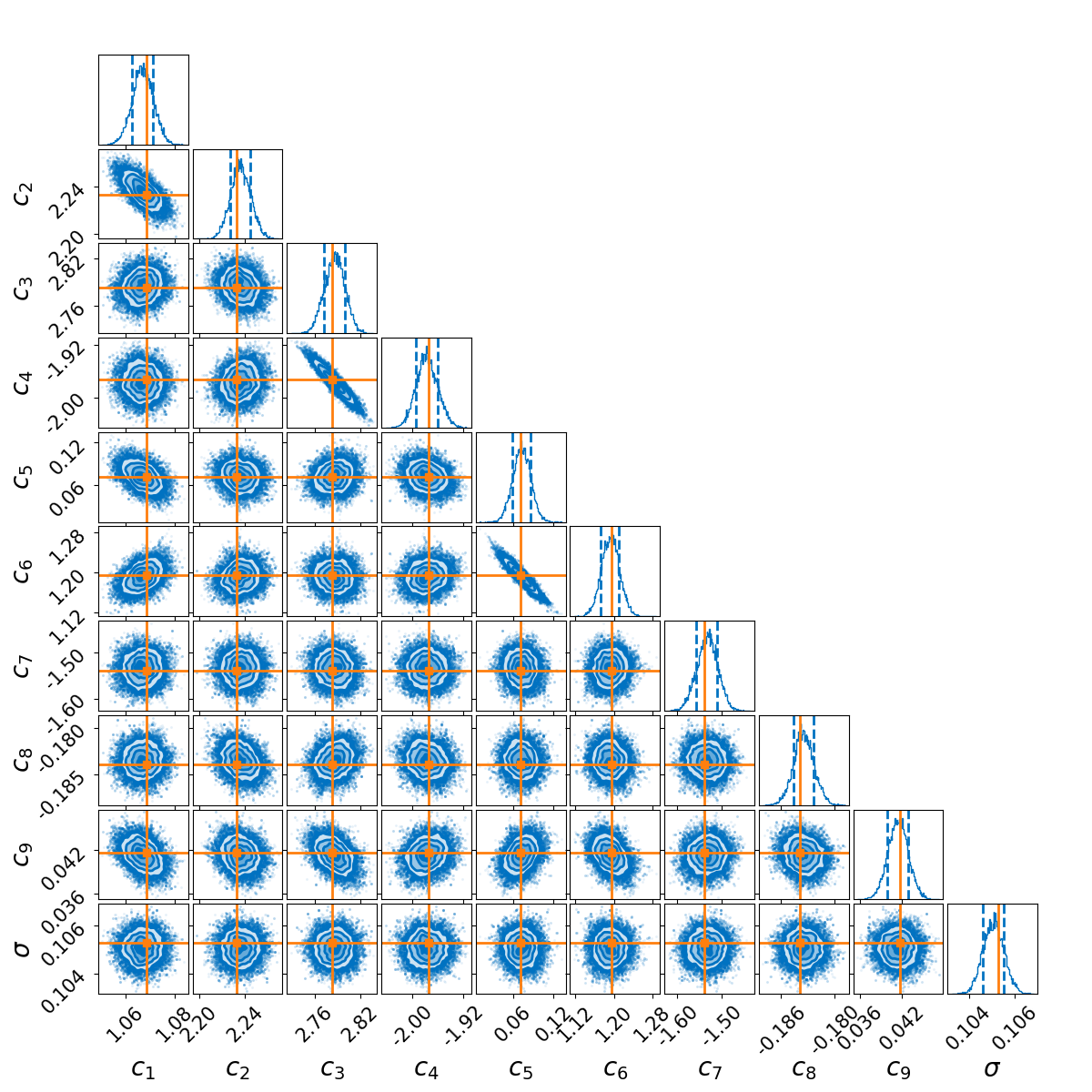
| 1.06 | 2.24 | 2.78 | -1.97 | 0.07 | 1.19 | -1.53 | -0.18 | 0.04 | 0.10 |
Inspired by this similarity between the extent of the cavity and that of the unstable region around the binary, and following a painstaking analysis of the dependence of the cavity size on the system parameters, we prescribe the cavity semi-major axis to be given by
| (11) |
where we propose to be the following semi-empirical formula describing the pericentre radius of the innermost stable orbit:
| (12) |
where is defined as
| (13) |
with , and . Note that corresponds to the Hill’s radius. The coefficients are dimensionless parameters that we constrain using Monte Carlo Markov Chain (MCMC) Bayesian inference. We discuss the role of each term in Sec. 4.4. Details about the MCMC procedure are reported in Appendix C, while the inferred values for are reported in Tab. 1.
The expression in Eq. (12) sums multiple physically motivated contributions that either increase or decrease the extent of the unstable region around the binary. Intuitively, each term has a geometrical interpretation that shifts the effective gravitational influence of the binary outward or inward. The term sets the reference length of the problem, . The coefficient is proportional to the size of the Hill sphere of the secondary mass for mass ratios , and remains constant for larger mass ratios66 6 Sticking to the geometrical interpretation, we speculate that this effect arises because, as the mass ratio increases, the centre of mass of the binary moves towards the secondary, reducing the effective reference length to the maximum distance of the secondary from the centre of mass of the binary, namely . This inward shift compensates for the increase in the Hill radius..
The coefficients and account for the binary eccentricity, which influences the location of the separation of the binary at apocentre (i.e., it marks the closest point to the cavity edge). Coefficients and account for the cavity eccentricity, as higher eccentricity brings the cavity pericentre closer to the binary apocentre. The value of suggests that the dependence on in is mainly quadratic. Coefficient captures the reduced stability of disc orbits when , that is when the cavity pericentre aligns with the binary apocentre, thereby increasing the pericentre radius of the last stable orbit. Finally, coefficients and , describe the mild dependence of the innermost stable orbit on viscosity and disc aspect ratio , with contributions to the value of of and , respectively.
We show in Fig. 6 a comparison between the theoretical prediction in Eq. 12 and the value extracted from the numerical simulation. Figure 7 shows the time evolution of and as a function of the binary mass ratio . Figure 8 shows violin plots of as a function of binary mass ratio and eccentricity . Violin plots highlight the variability of throughout the duration of the simulations. Theoretical predictions from Eq. (12) are shown as shaded regions in left panels and solid curves in right panels. Finally, Fig. 9 shows the dependence of on the relative orientation of binary and cavity pericentres .


4.4 Dependence on and


While larger values of lead to smaller innermost stable orbits (), consistent with previous studies, the small, but positive, value for indicates that larger values of pushes the innermost orbit outward, contrary to the expectation that thicker discs produce smaller cavities. We speculate that this effect arises because orbital stability (independent of hydrodynamics) sets the location of the innermost orbit, whereas the surface density maximum is displaced outward by approximately , which defines the reference length scale of stable density gradients in accretion discs. This result, while seemingly at odds with the past literature, where thicker discs are typically associated with smaller cavities, is actually consistent with the previous findings: disc eccentricity saturates to lower values in thicker discs, resulting ultimately in a smaller cavity. This behaviour is illustrated in Fig. 10, where simulations in Group 2 show that discs generally have larger and more eccentric cavities than the corresponding cases; nevertheless, for larger truncation is mildly more effective (), producing slightly larger values than for .
5 Discussion

5.1 The nature of tidal truncation
The results presented highlight that, for mass ratios , the mechanism of tidal truncation shares some important similarities with the dynamical processes that describe the stability of the orbits in the restricted three-body problem. In this framework, the pericentre distance is determined by celestial mechanical considerations, with mild corrections from hydrodynamic effects such as viscosity and pressure and acts on short, timescales, of the order of a few orbital times, as short-term processes. At the same time, viscosity and pressure, coupled with the action of individual resonances that gain strength within the disc, act on longer-timescales as long-term processes. More work is required to define whether tidal truncation consists of an interplay between short-term and long-term processes, or whether they operate independently as mutually exclusive mechanisms. The small contributions from coefficients and in Eq. (12) appear to suggest that, in our simulations, viscosity and disc thickness do not directly control truncation (which depends only weakly on them); rather, they indirectly yield smaller cavities by limiting the saturated eccentricity, an effect that could otherwise be misinterpreted as less efficient truncation. We cannot exclude that longer-term effects, that are not probed by our numerical setups, might lead to a stronger dependence on these parameters at later times.
In general, independently of the mechanism in action, cavity eccentricity appears to be a key element to determine the cavity size. However, its saturation level is known to be tightly linked to the thermodynamical treatment of the disc, including heating and cooling processes (113; 86). Moreover, we note that the assumption of a locally isothermal equation of state causes the angular momentum flux (70) and angular momentum deficit (116, AMD, ) to not be conserved. The flow instead conserves equivalent sound-speed weighted quantities. Since the disc eccentricity evolution is tied to the conservation of the AMD, the choice of a locally isothermal profile may play a role in shaping the specific eccentricity “history” of the cavity. Properly capturing these thermodynamic effects is therefore crucial for understanding the long-term evolution of cavity eccentricity, and thus the resulting disc truncation and structure.
When it is possible to reach a quasi-steady state, this is achieved through the balance between viscous stresses, gravitational forces and other angular momentum transport processes in the disc (e.g. transport and deposition through density waves 95, or disc winds 11) setting a constant angular momentum flux through the disc (e.g. 75). The ”balance” is global: the viscous torques, angular momentum transport through spiral density waves in the outer disc, and gravitational torque causes the material to be supplied to the cavity edge at a constant rate, and the dynamical chaos within the cavity funnels it into the sinks at the same rate. Indenpendently of whether orbital instability or other processes are dominant in shaping the cavity size, the unstable region represents a dynamical transition zone similar to the Innermost Stable Circular Orbit (ISCO) in black hole accretion discs. In this picture, within the unstable zone act an open boundary. Once material reaches its edge, it enters the chaotic zone where stable circular orbits no longer exist. At this point, the gas has two options (122): i) the material falls onto the sinks (or their circumstellar discs), which act as the ultimate sinks for both mass and angular momentum; ii) the material is thrown against the other edge of the cavity (in 3D simulations the material can also fly above the cavity wall and be ejected from the system). This is inherently consistent with the fact that circumbinary discs are known to be actively accreting systems.
We finally emphasize that when orbital instability is in action to define the cavity boundary, the binary continues to inject angular momentum and energy into the disc, while conversely experiencing a back-reaction torque through its coupling with density perturbations. Beyond the resonance overlap region, we expect individual resonances to become stronger as the disc eccentricity evolves, producing a slow long-term evolution towards the final disc geometric configuration, and, when possible, the reach of a quasi-steady state accretion flow.
5.2 Discrepancies and uncertainties
In general, from Fig. 6 we note that the prescription in Eq. (12) matches and from the simulations with an uncertainty of . This uncertainty increases for the largest cavities, that are associated with values of , in particular: simulations 05A6, 05B6, 1A6, 1B6. In these cases, cavities are mainly larger than predicted by Eq. (12), so that for these simulations it acts as a lower limit; this trend is visible in Fig. 6 where the prescription tends to underestimate cavity sizes.
In this context, it is important to distinguish between “systematic discrepancy” (persistent deviations from the expected value) and “variability” (fluctuations around a mean value). The “lower-limit” behaviour for is an example of a “systematic discrepancy” which, we speculate, has two possible interpretations. First, these discs are characterised by strong dynamical perturbations (see central panel of bottom row in Fig. 1): tidal streams stripped from one edge of the cavity collide with the opposite side (e.g., 110; 37), while steep eccentricity and pericentre longitude gradients can lead to shocks due to intersecting orbits (77; 112). These effects potentially deplete the material near the cavity edge, increasing the measured cavity size. In fact, Eq. (12) marks the innermost radius beyond which orbits remain stable, but it does not prevent other concurrent mechanisms from truncating or depleting the disc at larger radii. Second, the functional form of Eq. (12), where the factor dominates the dependence in Eq. (12), becomes inadequate for describing large values .
Regarding “variability”, secular and resonant effects produce oscillations of around a mean value. The full dynamics of circumbinary discs involves coupled secular and resonant oscillations of , and , that are not captured by Eq. (12). These appear as phased or antiphased periodic oscillation between both and across a median value (resonant) or oscillations of only at nearly constant (secular). In this framework, the innermost stable orbit sets a median theoretical cavity size , with the simulations exploring a range of values around this median.
Theoretical and numerical studies about orbital stability indicate that stable regions in the plane are inherently “ragged”, due to chaotic behaviour emerging where resonances overlap (e.g., see Fig. 3 of 109 or Fig. 6 in 1). This produces abrupt transitions between adjacent stable and unstable regions, causing variations in that cannot be captured by a smooth prescription such as Eq. (12).
Finally, to assess the reliability of our results, we compare the predictions from Eq. (12) with the simulations from two different works (85; 28) in Fig. 11. Despite differences in the approach used to measure the cavity size77 7 The location of the from the maximum value of the surface density profile in 85 and the location of in 28. (28, also have binaries with in their sample), the results in these works show remarkable agreement with Eq. (12).
6 Conclusion
In this work we have presented a suite of 80 numerical simulations and revisited the long-standing problem of tidal truncation in circumbinary discs, focusing in particular on the role played by disc eccentricity in setting the size and geometry of the central cavity. By analysing the extensive dataset of three-dimensional SPH simulations using the code phantom (92), spanning a wide range of binary and disc parameters, we show that:
(i) The growth of disc eccentricity and the expansion of the cavity occur concurrently and on comparable dynamical timescales, to the extent they can be considered tightly correlated. The often-reported slow evolution of the cavity size over hundreds or thousands of binary orbits needs to be interpreted considering this dependence on the cavity eccentricity.
(ii) The cavity size follows trends that strongly resemble those of chaotic orbit boundaries derived from purely gravitational considerations. Consistently with this insight, we introduced in Eq. (12) a semi-empirical formula that predicts the cavity size as a function of the instantaneous dynamical properties of the system. The prescription shows remarkable agreement within our own sample (Fig. 6) and other works (Fig. 11).
(iii) The impact of viscosity and pressure on the truncation radius is sub-dominant compared to that of the binary orbital parameters and disc eccentricity. The apparent dependence of cavity size on disc thickness reported in previous studies can be largely understood as an indirect effect: thicker, viscous discs tend to saturate at lower eccentricities, which in turn leads to smaller cavities.
(iv) Circumbinary discs should be regarded as fundamentally eccentric objects, whose global eccentric modes play an active role in shaping the disc structure. Treating eccentricity as a passive by-product of binary-disc interaction misses essential aspects of the dynamics.
(v) We speculate that processes analogous to orbital stability in the restricted three-body problem participate in tidal truncation acting on short-timescales. Whereas, on longer-timescales, the resonant-viscous torque balance from individual resonances is altered by the growth of disc eccentricity, impacting on the long-term evolution of the system. Our results do not allow us to determine whether these mechanisms undergo a complex interplay or whether they act as separate processes. Future work focusing on the long-term evolution of the system remains essential to fully disentangle their respective effects.
This paper is the first in a series devoted to understanding the dynamics of eccentric circumbinary discs. In forthcoming work, we will explore in more detail the excitation, saturation, and long-term evolution of eccentric eigenmodes, their coupling to binary orbital evolution, and the consequences for mass accretion, variability, and disc–binary angular momentum exchange. Together, these studies aim to build a coherent dynamical picture of circumbinary discs in which eccentricity is a central, predictive ingredient.
Acknowledgements.
The authors thank the anonymous referee for their comments that improved the manuscript. E.R. thanks Giuseppe Lodato, Daniel Price, Giovanni Rosotti, Nikolaos Georgakarakos, Alessia Franchini and Guglielmo Mastroserio for useful discussions. E.R. thanks Callum Fairbairn, Gordon Ogilvie, and Roman Rafikov for their comments on a preliminary version of the left panel of Fig. 3 during a visit to DAMTP (Cambridge) in November 2022. E.R. acknowledges financial support from the European Union’s Horizon Europe research and innovation programme under the Marie Skłodowska-Curie grant agreement No. 101102964 (ORBIT-D). ER, EL and GL acknowledge financial support from the European Research Council (ERC) under the European Union’s Horizon 2020 research and innovation programme (grant agreement No. 864965, PODCAST). ER and RA acknowledge financial support from the European Research Council (ERC) under the European Union’s Horizon 2020 research and innovation programme (grant agreement no. 681601, BuildingPlanS). ER also acknowledges support from the European Union (ERC Starting Grant DiscEvol, project number 101039651). This project has received funding from the European Union’s Horizon 2020 research and innovation programme under the Marie Skłodowska-Curie grant agreement No 823823 (DUSTBUSTERS). EL acknowledges funding from the Japan Society for the Promotion of Science through a JSPS International Research Fellowship. RA acknowledges funding from the Science & Technology Facilities Council (STFC) through Consolidated Grant ST/W000857/1. Views and opinions expressed are, however, those of the author(s) only and do not necessarily reflect those of the European Union or the European Research Council. The simulations performed for this paper used the DiRAC Data Intensive service at Leicester, operated by the University of Leicester IT Services, which forms part of the STFC DiRAC HPC Facility (www.dirac.ac.uk). Fig. 1 was created using splash (91). All the other figures were created using matplotlib python library (47).References
- [1] (2023) Stability of coorbital planets around binaries. A&A 680, pp. A29. External Links: 10.1051/0004-6361/202244329 Cited by: Appendix B, §2.1, §4.2.2, §5.2.
- [2] (2026) Numerical Insights into Disk Accretion, Eccentricity, and Kinematics in the Class 0 phase. arXiv e-prints, pp. arXiv:2601.08916. External Links: 10.48550/arXiv.2601.08916 Cited by: §2.2.
- [3] (2024) V892 Tau: A tidally perturbed circumbinary disc in a triple stellar system. A&A 687, pp. A311. External Links: 10.1051/0004-6361/202449683 Cited by: §1.
- [4] (2019) Gas flow and accretion via spiral streamers and circumstellar disks in a young binary protostar. Science 366 (6461), pp. 90-93. External Links: 10.1126/science.aaw3491 Cited by: §1.
- [5] (2015) Misaligned gas discs around eccentric black hole binaries and implications for the final-parsec problem. MNRAS 449 (1), pp. 65-76. External Links: 10.1093/mnras/stv128 Cited by: §1.
- [6] (2018) On the secular evolution of GG Tau A circumbinary disc: a misaligned disc scenario. MNRAS 480 (4), pp. 4738-4745. External Links: 10.1093/mnras/sty2179 Cited by: §1.
- [7] (2018) The Disk Substructures at High Angular Resolution Project (DSHARP). I. Motivation, Sample, Calibration, and Overview. ApJ 869 (2), pp. L41. External Links: 10.3847/2041-8213/aaf741 Cited by: §1, §2.2.
- [8] (1994) Dynamics of binary-disk interaction. 1: Resonances and disk gap sizes. ApJ 421, pp. 651-667. External Links: 10.1086/173679 Cited by: §1, §1, §2.1, §2.1, footnote 1.
- [9] (2013) Asymmetric transition disks: Vorticity or eccentricity?. A&A 553, pp. L3. External Links: 10.1051/0004-6361/201321125 Cited by: §2.2.
- [10] (2023) Structured Distributions of Gas and Solids in Protoplanetary Disks. In Protostars and Planets VII, (S. Inutsuka, Y. Aikawa, T. Muto, K. Tomida, and M. Tamura Eds.), pp. 423. External Links: 10.48550/arXiv.2210.13314 Cited by: §1.
- [11] (2016) Towards a Global Evolutionary Model of Protoplanetary Disks. ApJ 821 (2), pp. 80. External Links: 10.3847/0004-637X/821/2/80 Cited by: §5.1.
- [12] (1995) Modelling accretion in protobinary systems. MNRAS 277, pp. 362-376. External Links: 10.1093/mnras/277.2.362 Cited by: §3.1.
- [13] (2012) A Likely Close-in Low-mass Stellar Companion to the Transitional Disk Star HD 142527. ApJ 753 (2), pp. L38. External Links: 10.1088/2041-8205/753/2/L38 Cited by: §1.
- [14] (1999) Tidally Induced Gap Formation in Protostellar Disks: Gap Clearing and Suppression of Protoplanetary Growth. ApJ 514, pp. 344-367. External Links: 10.1086/306917 Cited by: §2.1.
- [15] (2020) Are the spiral arms in the MWC 758 protoplanetary disc driven by a companion inside the cavity?. MNRAS 498 (1), pp. 639-650. External Links: 10.1093/mnras/staa2468 Cited by: §2.2.
- [16] (2019) Signatures of an eccentric disc cavity: Dust and gas in IRS 48. MNRAS 490 (2), pp. 2579-2587. External Links: 10.1093/mnras/stz2770 Cited by: §2.2.
- [17] (2017) Testing dust trapping in the circumbinary disk around GG Tauri A. A&A 599, pp. A102. External Links: 10.1051/0004-6361/201629721 Cited by: §1.
- [18] (2021) Wide Dust Gaps in Protoplanetary Disks Induced by Eccentric Planets: A Mass-eccentricity Degeneracy. ApJ 922 (2), pp. 184. External Links: 10.3847/1538-4357/ac23d7 Cited by: §2.1.
- [19] (2024) Gravitational torque in circumbinary discs: global radial oscillations. MNRAS 528 (2), pp. 2358-2376. External Links: 10.1093/mnras/stae134 Cited by: §2.1.
- [20] (2019) SPHERE dynamical and spectroscopic characterization of HD 142527B. A&A 622, pp. A96. External Links: 10.1051/0004-6361/201833990 Cited by: §1.
- [21] (2024) Discs are born eccentric. A&A 689, pp. L9. External Links: 10.1051/0004-6361/202449610 Cited by: §2.2, §3.3, §3.3.
- [22] (2006) On the width and shape of gaps in protoplanetary disks. Icarus 181, pp. 587-604. External Links: 10.1016/j.icarus.2005.10.007 Cited by: §2.1, §2.1.
- [23] (2019) Resolved ALMA Continuum Image of the Circumbinary Ring and Circumstellar Disks in the L1551 IRS 5 System. ApJ 882 (1), pp. L4. External Links: 10.3847/2041-8213/ab39ea Cited by: §1.
- [24] (2019) Flybys in protoplanetary discs: I. Gas and dust dynamics. MNRAS 483 (3), pp. 4114-4139. External Links: 10.1093/mnras/sty3325 Cited by: §2.2.
- [25] (2025) The SHAMROCK code: I - smoothed particle hydrodynamics on GPUs. MNRAS 539 (1), pp. 1-33. External Links: 10.1093/mnras/staf444 Cited by: §3.1.
- [26] (2021) Outward Migration of Super-Jupiters. ApJ 918 (2), pp. L36. External Links: 10.3847/2041-8213/ac22af Cited by: §2.2.
- [27] (2022) A survey of disc thickness and viscosity in circumbinary accretion: Binary evolution, variability, and disc morphology. MNRAS 513 (4), pp. 6158-6176. External Links: 10.1093/mnras/stac935 Cited by: §2.2.
- [28] (2024) The Evolution of Accreting Binaries: From Brown Dwarfs to Supermassive Black Holes. ApJ 967 (1), pp. 12. External Links: 10.3847/1538-4357/ad2f1e Cited by: §2.1, §4.1, Figure 11, §5.2, footnote 7.
- [29] (2013) Gap Opening by Extremely Low-mass Planets in a Viscous Disk. ApJ 769, pp. 41. External Links: 10.1088/0004-637X/769/1/41 Cited by: §2.1.
- [30] (2024) The Santa Barbara Binary‑disk Code Comparison. ApJ 970 (2), pp. 156. External Links: 10.3847/1538-4357/ad5a7e Cited by: §2.2, §3.1, §4.1.
- [31] (2013) A limit on eccentricity growth from global 3D simulations of disc-planet interactions. MNRAS 428, pp. 3072-3082. External Links: 10.1093/mnras/sts254 Cited by: §2.2.
- [32] (2015) Precession and accretion in circumbinary discs: the case of HD 104237. MNRAS 448 (4), pp. 3545-3554. External Links: 10.1093/mnras/stv284 Cited by: §2.2.
- [33] (2006) Evolution of Giant Planets in Eccentric Disks. ApJ 652, pp. 1698-1714. External Links: 10.1086/508451 Cited by: §2.2.
- [34] (2013) Accretion into the central cavity of a circumbinary disc. MNRAS 436, pp. 2997-3020. External Links: 10.1093/mnras/stt1787 Cited by: §2.2.
- [35] (2018) Inferring giant planets from ALMA millimeter continuum and line observations in (transition) disks. A&A 612, pp. A104. External Links: 10.1051/0004-6361/201731390 Cited by: §2.1.
- [36] (2022) Density waves in protoplanetary discs excited by eccentric planets: linear theory. MNRAS 517 (2), pp. 2121-2130. External Links: 10.1093/mnras/stac2802 Cited by: §1.
- [37] (2014) Binary Black Hole Accretion from a Circumbinary Disk: Gas Dynamics inside the Central Cavity. ApJ 783, pp. 134. External Links: 10.1088/0004-637X/783/2/134 Cited by: §1, §2.2, §5.2.
- [38] (2023) The importance of live binary evolution in numerical simulations of binaries embedded in circumbinary discs. MNRAS 522 (1), pp. 1569-1574. External Links: 10.1093/mnras/stad1070 Cited by: §2.2, §3.1.
- [39] (2024) Empirical Stability Criteria for 3D Hierarchical Triple Systems. I. Circumbinary Planets. AJ 168 (5), pp. 224. External Links: 10.3847/1538-3881/ad7a78 Cited by: Figure 13, Appendix B, Appendix B, Appendix B, §2.1, Figure 3, Figure 5, §4.2.2, §4.2.2.
- [40] (1980) Disk-satellite interactions. ApJ 241, pp. 425-441. External Links: 10.1086/158356 Cited by: §1, §2.1.
- [41] (2006) The dynamics of eccentric accretion discs in superhump systems. MNRAS 368 (3), pp. 1123-1131. External Links: 10.1111/j.1365-2966.2006.10197.x Cited by: §2.2.
- [42] (2001) Planetary Torques as the Viscosity of Protoplanetary Disks. ApJ 552, pp. 793-802. External Links: 10.1086/320572 Cited by: §2.1.
- [43] (2025) Insights from Analytical Theory of Eccentric Circumbinary Disks. arXiv e-prints, pp. arXiv:2504.17658. External Links: 10.48550/arXiv.2504.17658 Cited by: §2.2, §4.1.
- [44] (2020) On the orbital evolution of binaries with circumbinary discs. A&A 641, pp. A64. External Links: 10.1051/0004-6361/202038548 Cited by: §2.2.
- [45] (2020) On the cavity size in circumbinary discs. MNRAS 498 (2), pp. 2936-2947. External Links: 10.1093/mnras/staa2536 Cited by: §1, §2.1.
- [46] (1999) Long-Term Stability of Planets in Binary Systems. AJ 117 (1), pp. 621-628. External Links: 10.1086/300695 Cited by: §2.1, §4.2.2.
- [47] (2007) Matplotlib: A 2D Graphics Environment. Computing in Science and Engineering 9, pp. 90-95. External Links: 10.1109/MCSE.2007.55 Cited by: §6.
- [48] (2019) A circumbinary protoplanetary disk in a polar configuration. Nature Astronomy 3, pp. 230-235. External Links: 10.1038/s41550-018-0667-x Cited by: §1.
- [49] (2020) Gap, shadows, spirals, streamers: SPHERE observations of binary-disk interactions in GG Tau A. arXiv e-prints, pp. arXiv:2005.09037. Cited by: §1.
- [50] (2006) Disk eccentricity and embedded planets. A&A 447, pp. 369-377. External Links: 10.1051/0004-6361:20053914 Cited by: §2.2, §2.2.
- [51] (1993) Two-dimensional Viscous Accretion Disk Models. II. On Viscous Overstability. ApJ 409, pp. 739. External Links: 10.1086/172703 Cited by: §2.2.
- [52] (2008) Simulations of eccentric disks in close binary systems. A&A 487 (2), pp. 671-687. External Links: 10.1051/0004-6361:200809953 Cited by: §2.2.
- [53] (2020) A triple-star system with a misaligned and warped circumstellar disk shaped by disk tearing. Science 369 (6508), pp. 1233-1238. External Links: 10.1126/science.aba4633 Cited by: §1.
- [54] (2023) Rejuvenating infall: a crucial yet overlooked source of mass and angular momentum. European Physical Journal Plus 138 (3), pp. 272. External Links: 10.1140/epjp/s13360-023-03880-y Cited by: §2.2.
- [55] (2016) An M-dwarf star in the transition disk of Herbig HD 142527. Physical parameters and orbital elements. A&A 590, pp. A90. External Links: 10.1051/0004-6361/201527863 Cited by: §1.
- [56] (2006) Viscous overstability and eccentricity evolution in three-dimensional gaseous discs. MNRAS 372 (4), pp. 1829-1839. External Links: 10.1111/j.1365-2966.2006.11014.x Cited by: §2.2.
- [57] (2023) 3D global simulations of accretion onto gap-opening planets: implications for circumplanetary disc structures and accretion rates. MNRAS 526 (4), pp. 5346-5364. External Links: 10.1093/mnras/stad3049 Cited by: §2.2.
- [58] (2021) The Architecture of the V892 Tau System: the Binary and its Circumbinary Disk. arXiv e-prints, pp. arXiv:2105.02918. Cited by: §1.
- [59] (2018) Gaps and Rings in an ALMA Survey of Disks in the Taurus Star-forming Region. ApJ 869 (1), pp. 17. External Links: 10.3847/1538-4357/aae8e1 Cited by: §1, §2.2.
- [60] (1991) A model for tidally driven eccentric instabilities in fluid disks. ApJ 381, pp. 259-267. External Links: 10.1086/170647 Cited by: §2.2.
- [61] (1991) Simulations of tidally driven eccentric instabilities with application to superhumps. ApJ 381, pp. 268-277. External Links: 10.1086/170648 Cited by: §2.2.
- [62] (2021) Dynamical structure of highly eccentric discs with applications to tidal disruption events. MNRAS 500 (3), pp. 4110-4125. External Links: 10.1093/mnras/staa3459 Cited by: §A.2.
- [63] (2022) Focusing of non-linear eccentric waves in astrophysical discs - II. Excitation and damping of tightly wound waves. MNRAS 510 (3), pp. 3460-3478. External Links: 10.1093/mnras/stab3605 Cited by: §2.2.
- [64] (1994) Eccentric Accretion Discs. MNRAS 266, pp. 583. External Links: 10.1093/mnras/266.3.583 Cited by: §2.2.
- [65] (2008) An Eccentric Circumbinary Accretion Disk and the Detection of Binary Massive Black Holes. ApJ 672, pp. 83-93. External Links: 10.1086/523869 Cited by: §2.2.
- [66] (2009) On the eccentricity of self-gravitating circumstellar disks in eccentric binary systems. A&A 508 (3), pp. 1493-1502. External Links: 10.1051/0004-6361/200912251 Cited by: §2.2.
- [67] (2020) Orbital and Mass Constraints of the Young Binary System IRAS 16293-2422 A. ApJ 897 (1), pp. 59. External Links: 10.3847/1538-4357/ab960b Cited by: §1.
- [68] (2017) Viscous hydrodynamics simulations of circumbinary accretion discs: variability, quasi-steady state and angular momentum transfer. MNRAS 466, pp. 1170-1191. External Links: 10.1093/mnras/stw3189 Cited by: §1, §2.2, §4.1, §4.1.
- [69] (2015) Tidal truncation of inclined circumstellar and circumbinary discs in young stellar binaries. MNRAS 452 (3), pp. 2396-2409. External Links: 10.1093/mnras/stv1450 Cited by: §1, §1, §2.1.
- [70] (2020) Planet-Disk Interaction in Disks with Cooling: Basic Theory. ApJ 892 (1), pp. 65. External Links: 10.3847/1538-4357/ab791a Cited by: §5.1.
- [71] (2004) A Planetesimal Accretion Zone in a Circumbinary Disk. ApJ 609, pp. 1065-1070. External Links: 10.1086/421342 Cited by: §4.1.
- [72] (1999) Solar system dynamics. Cited by: §1, §2.2.
- [73] (1996) SPH simulations of tidally unstable accretion discs in cataclysmic variables. MNRAS 279, pp. 402-414. External Links: 10.1093/mnras/279.2.402 Cited by: §2.2.
- [74] (2020) Long-lived Eccentric Modes in Circumbinary Disks. ApJ 905 (2), pp. 106. External Links: 10.3847/1538-4357/abc74c Cited by: §2.2, §2.2, §4.1, §4.1.
- [75] (2019) Hydrodynamics of Circumbinary Accretion: Angular Momentum Transfer and Binary Orbital Evolution. ApJ 871 (1), pp. 84. External Links: 10.3847/1538-4357/aaf867 Cited by: §4.1, §5.1.
- [76] (2024) The orbit of HD 142527 B is too compact to explain many of the disc features. A&A 683, pp. A6. External Links: 10.1051/0004-6361/202347748 Cited by: §1.
- [77] (2001) Non-linear fluid dynamics of eccentric discs. MNRAS 325, pp. 231-248. External Links: 10.1046/j.1365-8711.2001.04416.x Cited by: §2.2, §3.3, §4.1, §5.2.
- [78] (2019) Hamiltonian hydrodynamics of eccentric discs. MNRAS 483 (4), pp. 4453-4469. External Links: 10.1093/mnras/sty3436 Cited by: §A.2, §3.2, footnote 4.
- [79] (2008) 3D eccentric discs around Be stars. MNRAS 388 (3), pp. 1372-1380. External Links: 10.1111/j.1365-2966.2008.13484.x Cited by: §2.2.
- [80] (2023) Early Planet Formation in Embedded Disks (eDisk). I. Overview of the Program and First Results. ApJ 951 (1), pp. 8. External Links: 10.3847/1538-4357/acd384 Cited by: §2.2.
- [81] (1977) A model of accretion disks in close binaries.. ApJ 216, pp. 822-826. External Links: 10.1086/155526 Cited by: §2.1.
- [82] (2026) On Eccentric Protoplanetary Disks. I. How Eccentric are Planet-perturbed Disks?. ApJ 1000 (1), pp. 65. External Links: 10.3847/1538-4357/ae4339 Cited by: §2.2.
- [83] (2001) Orbital eccentricity growth through disc-companion tidal interaction. A&A 366, pp. 263-275. External Links: 10.1051/0004-6361:20000011 Cited by: §2.2.
- [84] (1977) Tidal torques on accretion discs in close binary systems.. MNRAS 181, pp. 441-454. External Links: 10.1093/mnras/181.3.441 Cited by: §2.1.
- [85] (2024) Viscous circumbinary protoplanetary discs - I. Structure of the inner cavity. MNRAS 532 (3), pp. 3166-3179. External Links: 10.1093/mnras/stae1689 Cited by: §1, §2.1, §4.1, Figure 11, §5.2, footnote 7.
- [86] (2025) Sculpting protoplanetary discs ─ modelling circumbinary cavities at observable scales with radiation hydrodynamics. MNRAS 544 (4), pp. 3312-3323. External Links: 10.1093/mnras/staf1876 Cited by: §2.2, §2.2, §5.1.
- [87] (2005) Circumstellar and circumbinary discs in eccentric stellar binaries. MNRAS 359 (2), pp. 521-530. External Links: 10.1111/j.1365-2966.2005.08905.x Cited by: §2.1, §2.1.
- [88] (2008) Geometrical and physical properties of circumbinary discs in eccentric stellar binaries. MNRAS 391 (2), pp. 815-824. External Links: 10.1111/j.1365-2966.2008.13916.x Cited by: §2.1, §2.1.
- [89] (2020) Hydrodynamical turbulence in eccentric circumbinary discs and its impact on the in situ formation of circumbinary planets. MNRAS 496 (3), pp. 2849-2867. External Links: 10.1093/mnras/staa1550 Cited by: §2.2.
- [90] (2018) Circumbinary, not transitional: on the spiral arms, cavity, shadows, fast radial flows, streamers, and horseshoe in the HD 142527 disc. MNRAS 477, pp. 1270-1284. External Links: 10.1093/mnras/sty647 Cited by: §2.2.
- [91] (2007) splash: An Interactive Visualisation Tool for Smoothed Particle Hydrodynamics Simulations. Publications of the Astronomical Society of Australia 24, pp. 159-173. External Links: 10.1071/AS07022 Cited by: §6.
- [92] (2018) Phantom: A Smoothed Particle Hydrodynamics and Magnetohydrodynamics Code for Astrophysics. PASA 35, pp. e031. External Links: 10.1017/pasa.2018.25 Cited by: §3.1, §3, §6.
- [93] (2018) Stability Limits of Circumbinary Planets: Is There a Pile-up in the Kepler CBPs?. ApJ 856 (2), pp. 150. External Links: 10.3847/1538-4357/aab264 Cited by: §2.1, §4.2.2.
- [94] (2002) Nonlinear Propagation of Planet-generated Tidal Waves. ApJ 569, pp. 997-1008. External Links: 10.1086/339399 Cited by: §1.
- [95] (2016) Protoplanetary Disk Heating and Evolution Driven by Spiral Density Waves. ApJ 831 (2), pp. 122. External Links: 10.3847/0004-637X/831/2/122 Cited by: §5.1.
- [96] (2017) On the origin of horseshoes in transitional discs. MNRAS 464, pp. 1449-1455. External Links: 10.1093/mnras/stw2456 Cited by: §2.2.
- [97] (2016) Suppression of the accretion rate in thin discs around binary black holes. MNRAS 460, pp. 1243-1253. External Links: 10.1093/mnras/stw1081 Cited by: §1, §2.2.
- [98] (2018) Eccentricity evolution during planet-disc interaction. MNRAS 474, pp. 4460-4476. External Links: 10.1093/mnras/stx3094 Cited by: §2.2, §2.2, §4.1, §4.1.
- [99] (2020) The evolution of large cavities and disc eccentricity in circumbinary discs. MNRAS 499 (3), pp. 3362-3380. External Links: 10.1093/mnras/staa2954 Cited by: Table 2, §1, §2.1, §2.2, §3.2, §4.1, §4.1.
- [100] (2021) Circumbinary and circumstellar discs around the eccentric binary IRAS 04158+2805 - a testbed for binary-disc interaction. MNRAS 507 (1), pp. 1157-1174. External Links: 10.1093/mnras/stab2179 Cited by: §1.
- [101] (2024) Probing the eccentricity in protostellar discs: Modelling kinematics and morphologies. A&A 686, pp. A264. External Links: 10.1051/0004-6361/202449583 Cited by: §A.1, §A.1, §A.2, §2.2, §4.1, footnote 4.
- [102] (2011) Spectral signatures of disk eccentricity in young binary systems. I. Circumprimary case. A&A 528, pp. A93. External Links: 10.1051/0004-6361/201016152 Cited by: §2.2.
- [103] (2024) Eccentricity and inclination of massive planets inside low-density cavities: results of 3D simulations. MNRAS 532 (3), pp. 3509-3525. External Links: 10.1093/mnras/stae1658 Cited by: §4.1.
- [104] (2016) The minimum mass of detectable planets in protoplanetary discs and the derivation of planetary masses from high-resolution observations. MNRAS 459, pp. 2790-2805. External Links: 10.1093/mnras/stw691 Cited by: §2.1.
- [105] (1981) Outer excretion disk around a close binary. Acta Astron. 31 (1), pp. 13-24. Cited by: §2.1.
- [106] (2025) Eccentric disks as a gateway to giant planet outward migration. A&A 704, pp. A78. External Links: 10.1051/0004-6361/202557059 Cited by: §2.2, §2.2.
- [107] (2022) Inward and outward migration of massive planets: moving towards a stalling radius. MNRAS 514 (4), pp. 5478-5492. External Links: 10.1093/mnras/stac1700 Cited by: §2.2, §2.2.
- [108] (1973) Black holes in binary systems. Observational appearance.. A&A 24, pp. 337-355. Cited by: §3.1, §3.2, footnote 9.
- [109] (2015) Chaotic Zones around Gravitating Binaries. ApJ 799 (1), pp. 8. External Links: 10.1088/0004-637X/799/1/8 Cited by: Appendix B, §5.2.
- [110] (2012) Three-dimensional Magnetohydrodynamic Simulations of Circumbinary Accretion Disks: Disk Structures and Angular Momentum Transport. ApJ 749, pp. 118. External Links: 10.1088/0004-637X/749/2/118 Cited by: §2.2, §5.2.
- [111] (2023) Preferential accretion and circumbinary disc precession in eccentric binary systems. MNRAS 518 (4), pp. 5059-5071. External Links: 10.1093/mnras/stac3263 Cited by: §2.2.
- [112] (2001) A Simple Family of Models for Eccentric Keplerian Fluid Disks. AJ 122 (5), pp. 2257-2266. External Links: 10.1086/323713 Cited by: §5.2.
- [113] (2022) How cooling influences circumbinary discs. A&A 664, pp. A157. External Links: 10.1051/0004-6361/202243472 Cited by: §2.2, §5.1.
- [114] (1992) The viscous evolution of elliptical accretion discs. MNRAS 255, pp. 92-104. External Links: 10.1093/mnras/255.1.92 Cited by: §2.2.
- [115] (2022) Eccentric Gap Induced by a Super-Jupiter-mass Planet. ApJ 925 (1), pp. 95. External Links: 10.3847/1538-4357/ac3af5 Cited by: §2.2.
- [116] (2016) Growth of eccentric modes in disc-planet interactions. MNRAS 458, pp. 3221-3247. External Links: 10.1093/mnras/stw521 Cited by: §1, §2.2, §3.2, §4.1, §4.1, §5.1.
- [117] (2017) Secular evolution of eccentricity in protoplanetary discs with gap-opening planets. MNRAS 467, pp. 4577-4590. External Links: 10.1093/mnras/stx426 Cited by: §3.3, §3.3.
- [118] (2019) A simplified model for the secular dynamics of eccentric discs and applications to planet-disc interactions. MNRAS 490 (3), pp. 4353-4365. External Links: 10.1093/mnras/stz2919 Cited by: §2.2.
- [119] (2017) Circumbinary discs: Numerical and physical behaviour. A&A 604, pp. A102. External Links: 10.1051/0004-6361/201730666 Cited by: §1, §2.1, §4.1, §4.1.
- [120] (2018) Migration of planets in circumbinary discs. A&A 616, pp. A47. External Links: 10.1051/0004-6361/201832804 Cited by: §2.1.
- [121] (2020) Gas-driven Inspiral of Binaries in Thin Accretion Disks. ApJ 900 (1), pp. 43. External Links: 10.3847/1538-4357/aba432 Cited by: §2.2.
- [122] (2022) How Binaries Accrete: Hydrodynamic Simulations with Passive Tracer Particles. ApJ 932 (1), pp. 24. External Links: 10.3847/1538-4357/ac6c2b Cited by: §5.1.
- [123] (2025) Suppressed Accretion onto Massive Black Hole Binaries Surrounded by Thin Disks. ApJ 984 (2), pp. 144. External Links: 10.3847/1538-4357/adc727 Cited by: §1.
- [124] (2016) A triple protostar system formed via fragmentation of a gravitationally unstable disk. Nature 538 (7626), pp. 483-486. External Links: 10.1038/nature20094 Cited by: §1.
- [125] (2024) Orbital dynamics in the GG Tau A system: Investigating its enigmatic disc. A&A 688, pp. A102. External Links: 10.1051/0004-6361/202348470 Cited by: §1, §2.2.
- [126] (1994) Eccentric-mode excitation of accretion discs.. MNRAS 266, pp. 35-49. External Links: 10.1093/mnras/266.1.35 Cited by: §2.2.
- [127] (2018) Inclination evolution of protoplanetary discs around eccentric binaries. MNRAS 473 (1), pp. 603-615. External Links: 10.1093/mnras/stx2375 Cited by: §1.
- [128] (2020) Eccentric tidal disruption event discs around supermassive black holes: dynamics and thermal emission. MNRAS 499 (4), pp. 5562-5577. External Links: 10.1093/mnras/staa3127 Cited by: §A.2.
- [129] (2018) The Disk Substructures at High Angular Resolution Project (DSHARP). VII. The Planet-Disk Interactions Interpretation. ApJ 869 (2), pp. L47. External Links: 10.3847/2041-8213/aaf744 Cited by: §2.1.
- [130] (2014) Dust Trapping by Vortices in Transitional Disks: Evidence for Non-ideal Magnetohydrodynamic Effects in Protoplanetary Disks. ApJ 795, pp. 53. External Links: 10.1088/0004-637X/795/1/53 Cited by: §2.2.
Appendix A Initialising an eccentric disc
A.1 Disc setup
In this Appendix we discuss how to initialise SPH particles to set up a Keplerian eccentric disc with eccentricity profile , longitude of pericentre profile and circular surface density profile (see Eq. (3) in Sec. 3.3). The geometry and local surface density distribution of the system are fully determined by these three quantities, and can be written as:
| (14) |
where is the determinant of the Jacobian matrix of the coordinate transform , is the orbital frequency for an orbit with semi-major axis and is the angular velocity along the orbit (101).
In phantom, for circular discs, the particles are initially distributed using an accept-reject approach that distributes the particles with the desired radial profile. To create the initial distribution of particles for an eccentric disc, we use a similar approach and proceed as follows to obtain the correct distribution (we assume ):
- 1.
We randomly generate a value of from a uniform distribution between inner and outer edges of the disc.
- 2.
We randomly generate a value of . To do so, we first generate from a uniform distribution a mean anomaly , we convert it to eccentric anomaly solving the equation using the Newton-Raphson method, and finally we convert to true anomaly
(15) and consequently set . This produces the correct azimuthal distribution.
- 3.
We generate randomly from a uniform distribution a final variable to accept or reject the couple we generated. If the value of satisfies
(16) the couple is accepted.
This criterion for acceptance is obtained by noting that the flux
(17) is constant along the orbit. Combining the expression for the mass contained within a certain radius with Eq. (14) and (17). Integrating across the whole orbit, we obtain that the amount of mass to be found within an annulus of thickness is
(18) from which Eq. (16) is obtained.
- 4.
Coordinate is sampled randomly from a Gaussian distribution with .
- 5.
Particle coordinates are then set using
(19) (20) (21) where is
(22) - 6.
Particle velocities are set assuming Keplerian orbits with no pressure corrections
(23) (24) (25) where is the orbital frequency.
In general this implementation neglects the different vertical displacement that is expected to occur at apocentre and pericentre (e.g. 101). Similarly, it neglects the vertical velocity resulting from the change of the vertical equilibrium along the orbit and the pressure corrections to the azimuthal velocity. We note this implementation is not supposed to represent the perfect equilibrium state of an eccentric disc, but a reasonably stable starting point from which the simulation can evolve to its most stable structure.
A.2 Setting up eccentric eigenmodes
To obtain the nonlinear eccentric eigenmodes used to generate the initial conditions for the Group 4 simulations we solve Equation (51) of 78 as a nonlinear eigenvalue problem for the precession frequency using a shooting method88 8 A version of the code used to solve the eigenvalue problem and generate the orbital elements and fluid properties can be found at: https://github.com/ElliotLynch/EccentricDiscSolvers.git.. We assume the surface density profile to be
| (26) |
where and , consistent with what assumed for the simulations but with the addition of an inner smoothing term, to have , and an exponential cutoff from , while the disc outer radius is . We use a locally isothermal temperature profile, defined prescribing , with and tuned to obtain the desired . We model the precession effects due to the binary quadrupole potential assuming it induces a forced precession
| (27) |
We impose free boundary conditions (128) at and . The theoretical eigenmodes are calculated assuming zero viscosity. We initialise our eigenmode simulations in the fundamental mode (no nodes in the eccentricity profile).
We note as a caveat that the resulting eigenmode is intended to serve as a reasonable initial guess for a stable eccentricity profile in the numerical simulations. We do not expect the eigenmode profiles obtained using the approach described above to be fully stable at the start of the simulations. The main aspects contributing to this are: i) the simulations employ a radial temperature profile, in contrast to the semi-major axis profile used to derive the theoretical eigenmodes; ii) the vertical velocities are not initialized to match the theoretical velocities expected from the onset of the breathing mode associated with the eccentricity profile (e.g. 62; 101); iii) the eigenmode profiles discussed in this Section and the simulations assume an initial cavity of in size, which does not correspond to the truncation radius that the binary would produce; iv) Finally, the simulations include viscosity, whereas the theoretical eigenmode profiles were derived assuming inviscid conditions.
Despite these caveats, we generally observe that the simulations relax to the appropriate eccentricity profile within a few tens of orbits, confirming that the eigenmode provides a reasonable initial guess. This can be seen in the fourth row of Fig. 2, which shows that the system precesses rigidly from the beginning of the numerical simulation and eventually settles into a stable configuration with the appropriate truncation radius.
Appendix B Dependence on different parameters in the vs , , ,
We report in Tab. 2, 3, 4, 5 the parameters used in the simulations. In Fig. 12 we mark in different colours the data points shown in Fig. 3 to highlight how different regions of the plot are associated to different parameters of the system. In Fig. 13 we show a detailed comparison between the predictions for from 39 and location of density maximum as discussed in Sec. 4.2.2.
Results from 5, 12, and 13 exhibit a visible correlation with the analytical prediction from 39, tracking the overall trend where more eccentric discs create cavities with larger semi-major axes. However, a closer inspection reveals that the data points do not strictly adhere to the theoretical boundary; rather, they exhibit moderate scatter both above and below the theoretical curve. In principle, given its definition of “orbital stability limit”, it would be reasonable to expect that this curve acts as a hard wall inside which no material should be observed on closed orbits; despite this, such deviations appears to be common.
We believe it is important to stress two considerations concerning the discrepancies described above. First, unlike the idealized test-particles modeled in pure -body frameworks, the gas in our hydrodynamical simulations is subject to internal pressure gradients and viscous diffusion (see Sec. 4.2.3), allowing gas elements to populate regions that would otherwise be dynamically unstable over long orbital timescales ( binary orbits). This effectively blurs the sharp cutoff predicted for pressureless, inviscid particles. Second, the analytical boundaries derived by 39 represent smooth parametric fits to an inherently chaotic phase space. In the restricted three-body problem, the transition between stable and unstable orbits mediated by mean-motion resonance overlap is highly irregular, typically characterised by a complex, “ragged” or sawtooth profile (e.g., see Fig. 3 of 109 or Fig. 6 in 1). This produces a scatter in values even for adjacent values.
| ID | |||||||
|---|---|---|---|---|---|---|---|
| 1A | 0.2 | 0.0 | 0.05 | 0.005 | 0 | 2 | 3506 |
| 1E | 0.2 | 0.0 | 0.05 | 0.1 | 0 | 2 | 4972 |
| 1G | 0.2 | 0.0 | 0.05 | 0.01 | 0 | 2 | 2201 |
| 1H | 0.2 | 0.0 | 0.05 | 0.01 | 0 | 2 | 2761 |
| 1N | 0.2 | 0.0 | 0.03 | 0.005 | 0 | 2 | 3001 |
| 1Z | 0.2 | 0.0 | 0.05 | 0.01 | 0 | 2 | 2001 |
| 2A | 0.1 | 0.0 | 0.05 | 0.005 | 0 | 2 | 3001 |
| 4A | 0.5 | 0.0 | 0.05 | 0.005 | 0 | 2 | 2606 |
| 4E30 | 0.5 | 0.0 | 0.055 | 0.1 | 0 | 2 | 785 |
| 4FF | 0.5 | 0.4 | 0.05 | 0.005 | 0 | 2 | 2431 |
| 4F | 0.5 | 0.1 | 0.05 | 0.005 | 0 | 2 | 2661 |
| 4N | 0.5 | 0.0 | 0.03 | 0.005 | 0 | 2 | 840 |
| 4Z | 0.5 | 0.0 | 0.05 | 0.01 | 0 | 2 | 2481 |
| 5A | 0.7 | 0.0 | 0.05 | 0.005 | 0 | 2 | 3001 |
| 5E | 0.7 | 0.0 | 0.05 | 0.1 | 0 | 2 | 3001 |
| 5Z | 0.7 | 0.0 | 0.05 | 0.01 | 0 | 2 | 2231 |
| 6A | 1.0 | 0.0 | 0.05 | 0.005 | 0 | 2 | 5939 |
| 6E | 1.0 | 0.0 | 0.05 | 0.1 | 0 | 2 | 2716 |
| 6Z | 1.0 | 0.0 | 0.05 | 0.01 | 0 | 2 | 3001 |
| 7A | 0.05 | 0.0 | 0.05 | 0.005 | 0 | 2 | 5106 |
| 8A | 0.075 | 0.0 | 0.05 | 0.005 | 0 | 2 | 3001 |
| 9A | 0.06 | 0.0 | 0.05 | 0.005 | 0 | 2 | 3001 |
| ID | |||||||
|---|---|---|---|---|---|---|---|
| 1A | 0.5 | 0.0 | 0.1 | 0.005 | 0 | 2 | 1450 |
| 2A | 0.5 | 0.1 | 0.1 | 0.005 | 0 | 2 | 1630 |
| 3A | 0.5 | 0.2 | 0.1 | 0.005 | 0 | 2 | 1715 |
| 3B | 0.5 | 0.2 | 0.05 | 0.005 | 0 | 2 | 592 |
| 3D | 0.5 | 0.2 | 0.05 | 0.05 | 0 | 2 | 226 |
| 4A | 0.5 | 0.3 | 0.1 | 0.005 | 0 | 2 | 1730 |
| 4B | 0.5 | 0.3 | 0.05 | 0.005 | 0 | 2 | 448 |
| 5A | 0.5 | 0.4 | 0.1 | 0.005 | 0 | 2 | 1691 |
| 5D | 0.5 | 0.4 | 0.05 | 0.05 | 0 | 2 | 143 |
| 6A | 0.5 | 0.5 | 0.1 | 0.005 | 0 | 2 | 1513 |
| 6B | 0.5 | 0.5 | 0.05 | 0.005 | 0 | 2 | 507 |
| 7A | 0.5 | 0.6 | 0.1 | 0.005 | 0 | 2 | 1441 |
| 7B | 0.5 | 0.6 | 0.05 | 0.005 | 0 | 2 | 376 |
| 7D | 0.5 | 0.7 | 0.05 | 0.05 | 0 | 2 | 143 |
| 8A | 0.5 | 0.7 | 0.1 | 0.005 | 0 | 2 | 1610 |
| 8B | 0.5 | 0.7 | 0.05 | 0.005 | 0 | 2 | 201 |
| 9A | 0.5 | 0.8 | 0.1 | 0.005 | 0 | 2 | 1923 |
| 9B | 0.5 | 0.8 | 0.05 | 0.005 | 0 | 2 | 333 |
| 9D | 0.5 | 0.8 | 0.05 | 0.015 | 0 | 2 | 273 |
| ID | |||||||
| 01A0 | 0.1 | 0.0 | 0.08 | 0.05 | 0.0 | 2 | 722 |
| 01A3 | 0.1 | 0.0 | 0.08 | 0.05 | 0.3 | 3 | 497 |
| 01A5 | 0.1 | 0.0 | 0.08 | 0.05 | 0.5 | 4 | 253 |
| 01A6 | 0.1 | 0.0 | 0.08 | 0.05 | 0.65 | 6 | 357 |
| 01B0 | 0.1 | 0.0 | 0.04 | 0.05 | 0.0 | 2 | 1000 |
| 01B3 | 0.1 | 0.0 | 0.04 | 0.05 | 0.3 | 3 | 822 |
| 01B5 | 0.1 | 0.0 | 0.04 | 0.05 | 0.5 | 4 | 231 |
| 01B6 | 0.1 | 0.0 | 0.04 | 0.05 | 0.65 | 6 | 218 |
| 05A0 | 0.5 | 0.0 | 0.08 | 0.05 | 0.0 | 2 | 571 |
| 05A3 | 0.5 | 0.0 | 0.08 | 0.05 | 0.3 | 3 | 517 |
| 05A5 | 0.5 | 0.0 | 0.08 | 0.05 | 0.5 | 4 | 161 |
| 05A6 | 0.5 | 0.0 | 0.08 | 0.05 | 0.65 | 6 | 243 |
| 05B0 | 0.5 | 0.0 | 0.04 | 0.05 | 0.0 | 2 | 558 |
| 05B3 | 0.5 | 0.0 | 0.04 | 0.05 | 0.3 | 3 | 507 |
| 05B5 | 0.5 | 0.0 | 0.04 | 0.05 | 0.5 | 4 | 300 |
| 05B6 | 0.5 | 0.0 | 0.04 | 0.05 | 0.65 | 6 | 220 |
| 1A0 | 1.0 | 0.0 | 0.08 | 0.05 | 0.0 | 2 | 514 |
| 1A3 | 1.0 | 0.0 | 0.08 | 0.05 | 0.3 | 3 | 484 |
| 1A5 | 1.0 | 0.0 | 0.08 | 0.05 | 0.5 | 4 | 157 |
| 1A6 | 1.0 | 0.0 | 0.08 | 0.05 | 0.65 | 6 | 299 |
| 1B0 | 1.0 | 0.0 | 0.04 | 0.05 | 0.0 | 2 | 631 |
| 1B2 | 1.0 | 0.0 | 0.05 | 0.05 | 0.2 | 2 | 931 |
| 1B3 | 1.0 | 0.0 | 0.04 | 0.05 | 0.3 | 3 | 632 |
| 1B5 | 1.0 | 0.0 | 0.04 | 0.05 | 0.5 | 4 | 341 |
| 1B6 | 1.0 | 0.0 | 0.04 | 0.05 | 0.65 | 6 | 321 |
| 1A0 | 1.0 | 0.0 | 0.1 | 0.05 | 0.0 | 2 | 139 |
| 1A2 | 1.0 | 0.0 | 0.1 | 0.05 | 0.2 | 2 | 196 |
| 1A4 | 1.0 | 0.0 | 0.1 | 0.05 | 0.4 | 2 | 124 |
| 1A5 | 1.0 | 0.0 | 0.1 | 0.05 | 0.5 | 2 | 132 |
| 1B0 | 1.0 | 0.0 | 0.05 | 0.05 | 0.0 | 2 | 143 |
| 1B2 | 1.0 | 0.0 | 0.05 | 0.05 | 0.2 | 2 | 931 |
| 1B4 | 1.0 | 0.0 | 0.05 | 0.05 | 0.4 | 2 | 139 |
| 1B5 | 1.0 | 0.0 | 0.05 | 0.05 | 0.5 | 2 | 110 |
| ID | |||||||
|---|---|---|---|---|---|---|---|
| 01A3 | 0.1 | 0.0 | 0.08 | 0.01 | 0.3 | 3 | 3128 |
| 01B3 | 0.1 | 0.0 | 0.04 | 0.01 | 0.3 | 3 | 1588 |
| 05A3 | 0.5 | 0.0 | 0.08 | 0.01 | 0.3 | 3 | 3401 |
| 05B3 | 0.5 | 0.0 | 0.04 | 0.01 | 0.3 | 3 | 1639 |
| 1A3 | 1.0 | 0.0 | 0.08 | 0.01 | 0.3 | 3 | 1497 |
| 1B3 | 1.0 | 0.0 | 0.04 | 0.01 | 0.3 | 3 | 2041 |


Appendix C MCMC Cornerplot
We obtain the values of in Eq. (12) using Bayesian inference by running an MCMC analysis on the dataset. We adopt a Gaussian likelihood with standard deviation , which is inferred as a free parameter:
| (28) |
where , is the pericentre radius of the -th simulation snapshot in our dataset, is the corresponding pericentre radius predicted using Eq. (12), and is the total number of simulation snapshots. We assume uniform priors for all coefficients, and run the MCMC for steps with 20 walkers, discarding the first steps.
We report in Tab. 1 the values of the parameters and corresponding to the maximum likelihood from the MCMC procedure. Figure 14 shows posterior distributions for parameters in Eq. (12).