跳到论文正文
W Papers独立论文阅读器 arXiv:2606.26752 论文正文 计算阅读时间 · 0%
引用这篇论文根据当前论文元数据生成,正式投稿前建议核对。


Global analysis of a minimally extended scotogenic model

Huchan Lee Email: huchanlee@seoultech.ac.kr Affiliation: School of Natural Science, Seoul National University of Science and Technology, Gongreung-ro 232, Seoul 01811, Republic of Korea    Sin Kyu Kang Email: skkang@seoultech.ac.kr Affiliation: School of Natural Science, Seoul National University of Science and Technology, Gongreung-ro 232, Seoul 01811, Republic of Korea
(July 5, 2026)
Abstract

We perform a global analysis of a minimally extended scotogenic model motivated by observed non-zero neutrino masses, viable dark matter (DM) candidates, and the instability of the Standard Model (SM) vacuum at high-energies. We examine the bounded-from-below conditions, vacuum stability, and RG-driven perturbativity bounds arising from the extended scalar sector, alongside a comprehensive set of flavor and electroweak (EW) precision observables - including the muon anomalous magnetic moment Δ​aμ\Delta a_{\mu}, the radiative decays ℓα→ℓβ​γ\ell_{\alpha}\rightarrow\ell_{\beta}\gamma and ℓα→3​ℓβ\ell_{\alpha}\rightarrow 3\ell_{\beta}, and the μ→e\mu\rightarrow e conversion rate, the oblique parameters, and leptonic decays of ZZ and HH bosons. A numerical scan reveals four notable features: the DESI BAO bound would rule out the inverted hierarchy if confirmed by other experiments; the oblique parameters are projected to be within the reach of future precision measurements; the viable fermionic DM candidate mass lies in the range 120−350​GeV120-350\operatorname{GeV}, while the CP-odd scalar is constrained to 350−600​GeV350-600\operatorname{GeV}; and our result on Z→InvisibleZ\rightarrow\operatorname{Invisible} is compatible with the world average at the 3​σ3\sigma level and is favored by the recent ATLAS measurement at the 3​σ3\sigma level.

I Introduction

The Standard Model (SM) has successfully described a wide range of phenomena with remarkable precision. Despite its great success, several fundamental observations remain unexplained within the SM framework, most notably the experimentally established neutrino masses and mixing, and the existence of dark matter (DM). The original scotogenic model 76, which simultaneously accounts for both of these phenomena, has therefore attracted significant attention. The scotogenic model, however, inherits a theoretical tension already present in the SM: the metastability of the electroweak (EW) vacuum 67. For the experimentally measured values of the Higgs boson and top quark masses, the renormalization group (RG) evolution of the SM Higgs quartic coupling drives it to negative values at scales of order 109​GeV10^{9}\operatorname{GeV}, signaling an instability of the scalar potential at high energies. In this work, we address this issue by extending the scotogenic scalar sector with an additional scalar field that mixes with the SM Higgs. The presence of this new scalar modifies the RG running of the quartic couplings, allowing them to remain positive across the energy scales where the theory remains perturbative. Consequently, EW vacuum stability is restored through the combined effects of the scalar mixing and RG evolution of the quartic couplings.

This limitation motivates a minimal extension of the original scotogenic model, designed to simultaneously address the EW vacuum stability issue while preserving the model’s predictivity and phenomenological viability. We begin by discussing the neutrino mass generation mechanism under both normal and inverted hierarchies. Cosmological observations from the Planck collaboration place a stringent 95%95\% confidence level (C.L.) upper bound on the sum of the three active neutrino masses 13:

∑i=13mνi≤10−10​GeV.\sum_{i=1}^{3}m_{\nu_{i}}\leq 10^{-10}\operatorname{GeV}. (1)

We then identify the viable parameter space for each hierarchy subject to all relevant theoretical constraints, including bounded-from-below (BFB) conditions, vacuum stability, and perturbativity bounds induced by RG running. Within this framework, we compute the precision and flavor observables — namely, the radiative decays ℓα→ℓβ​γ\ell_{\alpha}\rightarrow\ell_{\beta}\gamma and ℓα→3​ℓβ\ell_{\alpha}\rightarrow 3\ell_{\beta}, the conversion ratio of μ→e\mu\rightarrow e, the oblique parameters, and the leptonic and invisible decay modes of the ZZ and Higgs bosons (Z/H→ℓ¯α​ℓβ,ν¯​νZ/H\rightarrow\overline{\ell}_{\alpha}\ell_{\beta},\,\overline{\nu}\nu) — while performing a full renormalization analysis without imposing simplifying assumptions on the scalar sector. In this model, the SM scalar sector is extended by an additional scalar field that acquires a nonzero vacuum expectation value (VEV) and mixes with the SM Higgs. Consequently, tadpole contributions cannot be absorbed solely through counter-terms, as is conventionally done in the SM. We therefore adopt an alternative tadpole scheme 58 in which one-particle-irreducible (1PI) contributions are consistently combined with explicit tadpole insertions wherever they arise. Within this framework, we compute each precision observable in both the SM and the present model, and take their differences as a measure of the predicted new physics (NP) effects.

Given the flavor observables and constraints arising from both the lepton and scalar sectors, we perform a numerical parameter scan. In view of the complexity and high-dimensionality of the parameter space, we employ a Markov Chain Monte Carlo (MCMC) algorithm 77 constrained by two key observables - the SM Higgs mass at one-loop and the relic density - rather than a random scan. A distinguishing feature of this work is the absence of a large-Yukawa driven analysis. Numerous previous studies have attempted to accommodate the muon anomalous magnetic moment at the 4.2​σ4.2\sigma level or above, based on the 2020 White paper 20, which generically requires Yukawa couplings of order unity and consequently produces a significant enhancement of other flavor observables. Such a large-Yukawa-driven analysis is, however, disfavored by the RG analysis detailed in the following section. Furthermore, the 2025 WP paper 17, incorporating a revised hadronic vaccum polarization (HVP) contribution evaluated from lattice QCD, reports an updated SM muon g−2g-2 prediction yielding:

Δ​aμ=aμexp−aμSM=38​(63)×10−11,\Delta a_{\mu}=a_{\mu}^{\operatorname{exp}}-a_{\mu}^{\operatorname{SM}}=38(63)\times 10^{-11}, (2)

corresponding to a 0.6​σ0.6\sigma deviation, which indicates no statistically significant tension between the SM prediction and the experimental world average. It is therefore of considerable importance to identify viable directions for New Physics (NP) searches under these circumstances, and in this work we investigate observables accessible in near-future experiments without invoking artificially enhanced parameters.

This work is organized as follows: Section II introduces the model under study, including the neutrino mass generation mechanism for both mass hierarchies and the DM phenomenology. Section III examines the constraints arising from the extended scalar sector, with particular emphasis on the BFB conditions, vacuum stability, and RG-driven perturbativity bounds. Section IV is devoted to flavor and EW precision observables. In Section V, we present the numerical analysis and discuss the resulting phenomenological implications. Finally, Section VI summarizes our main findings. Appendix A provides details of the Casas-Ibarra parameterization employed in this work. Appendix B presents the self-energy contributions incorporating tadpole insertions. Appendix C details the derivation of the BFB conditions. Finally, Appendix D collects all the RGEs used in this analysis.

II Model

The model under study is seen in Table 1.

Field QiQ_{i} uicu_{i}^{c} dicd_{i}^{c} LiL_{i} eice_{i}^{c} NicN_{i}^{c} HH η\eta SS
S​U​(3)CSU(3)_{C} 𝟑\mathbf{3} 𝟑¯\mathbf{\bar{3}} 𝟑¯\mathbf{\bar{3}} 𝟏\mathbf{1} 𝟏\mathbf{1} 𝟏\mathbf{1} 𝟏\mathbf{1} 𝟏\mathbf{1} 𝟏\mathbf{1}
S​U​(2)LSU(2)_{L} 𝟐\mathbf{2} 𝟏\mathbf{1} 𝟏\mathbf{1} 𝟐\mathbf{2} 𝟏\mathbf{1} 𝟏\mathbf{1} 𝟐\mathbf{2} 𝟐\mathbf{2} 𝟏\mathbf{1}
U​(1)YU(1)_{Y} 16\frac{1}{6} −23-\frac{2}{3} 13\frac{1}{3} −12-\frac{1}{2} 11 00 12\frac{1}{2} 12\frac{1}{2} 00
Z2Z_{2} 11 11 11 11 11 −1-1 11 −1-1 11
U​(1)XU(1)_{X} 00 00 00 −1-1 11 11 00 00 −2-2
Table 1: Particle content of the minimally extended scotogenic model. The new fermions Ni​RN_{iR} are right-handed (RH) neutrinos, with the index i=1,2,3i=1,2,3. The Z2Z_{2} charge 1​(−1)1(-1) corresponds to even(odd) parity, respectively. Compared to the original scotogenic model, the present model is extended by an additional gauge-singlet scalar SS, which acquires a nonzero VEV, as well as a global U⁡(1)X\operatorname{U}\left(1\right)_{X} symmetry. All the fermions are two-component left-chiral Weyl spinors.

The renormalizable Lagrangian with the particle content reads in Equation 3:

ℒren=yu​Qi​H~​uic−yd​Qi​H​dic−ye​Li​H​eic+gX​Li​η​Nic+gR2​S​Nic​Nic+h.c..\mathcal{L_{\operatorname{ren}}}=y_{u}Q_{i}\widetilde{H}u_{i}^{c}-y_{d}Q_{i}Hd_{i}^{c}-y_{e}L_{i}He_{i}^{c}+g_{X}L_{i}\eta N_{i}^{c}+\frac{g_{R}}{2}SN_{i}^{c}N_{i}^{c}+\operatorname{h.c.}. (3)

where yu,d,ey_{u,d,e} denote the SM Yukawa couplings while gX,Rg_{X,R} are new Yukawa couplings associated with the extended sector. These new couplings are constrained by neutrino oscillation data. Here, we introduce the global U​(1)XU\left(1\right)_{X} symmetry in order to generate RH neutrino mass terms through Yukawa-like interactions and to make explicit how masses are assigned to the new scalar fields. This approach has the advantage that the associated Yukawa couplings can be consistently included in the RG evolution of all free parameters, which will be detailed in Section III.3, thereby enabling a more comprehensive analysis. The mass matrix for the RH neutrinos Ni​RN_{iR} is parameterized in the flavor basis and the diagonalized RH mass matrix is written in the physical basis of χi(i=1,2,3)\chi_{i}\left(i=1,2,3\right):

Mχflavor=12​gRi​j​vSi,j=1,2,3,Uχ,∗​Mχflavor​Uχ,†=Mχdiag.\begin{split}M_{\chi}^{\operatorname{flavor}}=\frac{1}{\sqrt{2}}g_{R}^{ij}v_{S}\quad\text{$i,j=1,2,3$},\quad U^{\chi,*}M_{\chi}^{\operatorname{flavor}}U^{\chi,\dagger}=M_{\chi}^{\operatorname{diag}}.\end{split} (4)

where UχU^{\chi} is a unitary mixing matrix which diagonalize the Majorana RH neutrino mass matrix. The extended scalar potential is given in Equation 5:

Vren=−μH2​H†​H+μη2​η†​η−μS2​S∗​S−12​μsb2​(S2+S∗,2)+14​λ1​(H†​H)2+14​λ2​(η†​η)2+λ3​(H†​H)​(η†​η)+λ4​(H†​η)​(η†​H)+14λ5[(η†H)2+h.c.]+14λ6(S∗S)2+λ7(H†H)(S∗S)+λ8(η†η)(S∗S)\begin{split}V_{\operatorname{ren}}&=-\mu_{H}^{2}H^{\dagger}H+\mu_{\eta}^{2}\eta^{\dagger}\eta-\mu_{S}^{2}S^{*}S-\frac{1}{2}\mu_{\operatorname{sb}}^{2}(S^{2}+S^{*,2})\\ &+\frac{1}{4}\lambda_{1}(H^{\dagger}H)^{2}+\frac{1}{4}\lambda_{2}(\eta^{\dagger}\eta)^{2}+\lambda_{3}(H^{\dagger}H)(\eta^{\dagger}\eta)+\lambda_{4}(H^{\dagger}\eta)(\eta^{\dagger}H)\\ &+\frac{1}{4}\lambda_{5}\left[(\eta^{\dagger}H)^{2}+h.c.\right]+\frac{1}{4}\lambda_{6}(S^{*}S)^{2}+\lambda_{7}(H^{\dagger}H)(S^{*}S)+\lambda_{8}(\eta^{\dagger}\eta)(S^{*}S)\end{split} (5)

where μH,η,S\mu_{H,\eta,S} are dimensionful mass parameters, and μsb\mu_{\operatorname{sb}} is a soft-breaking term that gives rise to nonzero masses for the CP-odd scalar. The scalar fields are decomposed as follows after spontaneous symmetry breaking (SSB):

H=(G+12​(v+ϕH0+i​σH0)),η=(η+12​(ηR+i​ηI)),S=12(vS+ϕS+i​σS),\begin{split}H=\begin{pmatrix}G^{+}\\ \frac{1}{\sqrt{2}}\left(v+\phi_{H^{0}}+i\sigma_{H^{0}}\right)\end{pmatrix},\quad\eta=\begin{pmatrix}\eta^{+}\\ \frac{1}{\sqrt{2}}\left(\eta_{R}+i\eta_{I}\right)\end{pmatrix},\quad S=\frac{1}{\sqrt{2}}\begin{pmatrix}v_{S}+\phi_{S}+i\sigma_{S}\end{pmatrix},\end{split} (6)

here, G+G^{+} is the would-be Goldstone boson associated with the SM WW gauge boson, η+\eta^{+} is a physical charged scalar field, vv is the SM VEV, vSv_{S} is the VEV of the new singlet scalar SS. The fields ϕ\phi and σ\sigma correspond to the CP-even and -odd components of the scalars, respectively. The mass matrix for the CP-even scalars in the flavor basis (ϕH0,ϕS)\left(\phi_{H^{0}},\phi_{S}\right) is:

MCP−even2=(14​(−4​μH2+3​λ1​v2+2​λ7​vS2)λ7​v​vSλ7​v​vS14​(−4​(μS2+μsb2)+2​λ7​v2+3​λ6​vS2))\begin{split}M_{\operatorname{CP-even}}^{2}&=\begin{pmatrix}\frac{1}{4}(-4\mu_{H}^{2}+3\lambda_{1}v^{2}+2\lambda_{7}v_{S}^{2})&\lambda_{7}vv_{S}\\ \lambda_{7}vv_{S}&\frac{1}{4}(-4(\mu_{S}^{2}+\mu_{\operatorname{sb}}^{2})+2\lambda_{7}v^{2}+3\lambda_{6}v_{S}^{2})\end{pmatrix}\end{split} (7)

and the diagonalized CP-even mass matrix by a unitary mixing matrix UHU^{H} is given in the physical basis of hi(i=1,2)h_{i}\left(i=1,2\right):

UH​MCP−even2​UH,T=MCP−evendiag,2,(h1,h2)T=UHT​(ϕH0,ϕS)T.U^{H}M_{\operatorname{CP-even}}^{2}U^{H,T}=M_{\operatorname{CP-even}}^{\operatorname{diag},2},\quad\left(h_{1},h_{2}\right)^{T}=U_{H}^{T}\left(\phi_{H^{0}},\phi_{S}\right)^{T}. (8)

In the CP-odd sector, the mixing matrix is the identity matrix, so the CP-odd scalars in the flavor basis (σH0,σS)\left(\sigma_{H^{0}},\sigma_{S}\right) coincide with the mass eigenstates a1a_{1} and a2a_{2}, where a1a_{1} is the would-be Goldstone boson of the ZZ and a2a_{2} is a physical CP-odd scalar of the extended sector.

II.1 Neutrino mass generation

The active neutrino masses are generated at the one-loop level through interactions with new particles shown in Figure 1.

Figure 1: Neutrino mass generation diagram at the one-loop level. Here, χk\chi_{k} denote the physical RH Majorana neutrinos (k=1,2,3)\left(k=1,2,3\right) and ηR,I\eta_{R,I} are the physical CP-even and -odd components of the scalar η\eta, respectively

The one-loop neutrino mass matrix MνM_{\nu} can be written as:

Mν=gXT​ML​gX.M_{\nu}=g_{X}^{T}M_{L}g_{X}. (9)

where gXg_{X} is the 3×33\times 3 Yukawa coupling constants and MLM_{L} is a symmetric 3×33\times 3 one-loop mass matrix given in Equation 10:

ML11=12​∑k=13(bloop​(ηR,k)−bloop​(ηI,k))​(U(k,1)χ,∗)2,ML22=12​∑k=13(bloop​(ηR,k)−bloop​(ηI,k))​(U(k,2)χ,∗)2,ML33=12​∑k=13(bloop​(ηR,k)−bloop​(ηI,k))​(U(k,3)χ,∗)2,ML12=ML21=12​∑k=13(bloop​(ηR,k)−bloop​(ηI,k))​(U(k,1)χ,∗)​(U(k,2)χ,∗),ML13=ML31=12​∑k=13(bloop​(ηR,k)−bloop​(ηI,k))​(U(k,1)χ,∗)​(U(k,3)χ,∗),ML23=ML32=12​∑k=13(bloop​(ηR,k)−bloop​(ηI,k))​(U(k,2)χ,∗)​(U(k,3)χ,∗),\begin{split}M_{L}^{11}&=\frac{1}{2}\sum_{k=1}^{3}\left(b_{\operatorname{loop}}(\eta_{R},k)-b_{\operatorname{loop}}(\eta_{I},k)\right)\left(U_{(k,1)}^{\chi,*}\right)^{2},\\ M_{L}^{22}&=\frac{1}{2}\sum_{k=1}^{3}\left(b_{\operatorname{loop}}(\eta_{R},k)-b_{\operatorname{loop}}(\eta_{I},k)\right)\left(U_{(k,2)}^{\chi,*}\right)^{2},\\ M_{L}^{33}&=\frac{1}{2}\sum_{k=1}^{3}\left(b_{\operatorname{loop}}(\eta_{R},k)-b_{\operatorname{loop}}(\eta_{I},k)\right)\left(U_{(k,3)}^{\chi,*}\right)^{2},\\ M_{L}^{12}=M_{L}^{21}&=\frac{1}{2}\sum_{k=1}^{3}\left(b_{\operatorname{loop}}(\eta_{R},k)-b_{\operatorname{loop}}(\eta_{I},k)\right)\left(U_{(k,1)}^{\chi,*}\right)\left(U_{(k,2)}^{\chi,*}\right),\\ M_{L}^{13}=M_{L}^{31}&=\frac{1}{2}\sum_{k=1}^{3}\left(b_{\operatorname{loop}}(\eta_{R},k)-b_{\operatorname{loop}}(\eta_{I},k)\right)\left(U_{(k,1)}^{\chi,*}\right)\left(U_{(k,3)}^{\chi,*}\right),\\ M_{L}^{23}=M_{L}^{32}&=\frac{1}{2}\sum_{k=1}^{3}\left(b_{\operatorname{loop}}(\eta_{R},k)-b_{\operatorname{loop}}(\eta_{I},k)\right)\left(U_{(k,2)}^{\chi,*}\right)\left(U_{(k,3)}^{\chi,*}\right),\end{split} (10)

and the loop function bloopb_{\operatorname{loop}} is defined as:

bloop​(ϕ,k)=116​π2​MχkMϕ2−Mχk,2​(Mϕ2​ln⁡Mϕ2Mχk,2)b_{\operatorname{loop}}\left(\phi,k\right)=\frac{1}{16\pi^{2}}\frac{M_{\chi}^{k}}{M_{\phi}^{2}-M_{\chi}^{k,2}}\left(M_{\phi}^{2}\ln{\frac{M_{\phi}^{2}}{M_{\chi}^{k,2}}}\right) (11)

where ϕ=ηR,I\phi=\eta_{R,I}. The coupling matrix gXg_{X} can be expressed using the Casas-Ibarra parameterization 39, which is detailed in Appendix A. The recent neutrino experimental data is given in Table 2.

Normal hierarchy Inverted hierarchy
1​σ1\sigma range 3​σ3\sigma range 1​σ1\sigma range 3​σ3\sigma range
sin2θ12\sin^{2}_{\theta_{12}} 0.3088−0.0066+0.00670.3088_{-0.0066}^{+0.0067} 0.2893→0.32950.2893\rightarrow 0.3295 0.3088−0.0066+0.00670.3088_{-0.0066}^{+0.0067} 0.2893→0.32950.2893\rightarrow 0.3295
θ12/∘\theta_{12}/^{\circ} 33.76−0.41+0.4233.76_{-0.41}^{+0.42} 32.54→35.0332.54\rightarrow 35.03 33.76−0.41+0.4233.76_{-0.41}^{+0.42} 32.54→35.0332.54\rightarrow 35.03
sin2θ23\sin^{2}_{\theta_{23}} 0.470−0.014+0.0170.470_{-0.014}^{+0.017} 0.432→0.5870.432\rightarrow 0.587 0.555−0.016+0.0130.555_{-0.016}^{+0.013} 0.437→0.5900.437\rightarrow 0.590
θ23/∘\theta_{23}/^{\circ} 43.27−0.82+1.0043.27_{-0.82}^{+1.00} 41.11→50.0241.11\rightarrow 50.02 48.15−0.92+0.7548.15_{-0.92}^{+0.75} 41.40→50.2141.40\rightarrow 50.21
sin2θ13\sin^{2}_{\theta_{13}} 0.02249−0.00057+0.000570.02249_{-0.00057}^{+0.00057} 0.02070→0.024200.02070\rightarrow 0.02420 0.02261−0.00056+0.000560.02261_{-0.00056}^{+0.00056} 0.02091→0.024330.02091\rightarrow 0.02433
θ13/∘\theta_{13}/^{\circ} 8.62−0.11+0.118.62_{-0.11}^{+0.11} 8.27→8.958.27\rightarrow 8.95 8.65−0.11+0.118.65_{-0.11}^{+0.11} 8.31→8.978.31\rightarrow 8.97
δC​P/∘\delta_{CP}/^{\circ} 207−20+23207_{-20}^{+23} 114→405114\rightarrow 405 283−28+24283_{-28}^{+24} 202→347202\rightarrow 347
Δ​m21210−5​eV2\frac{\Delta m_{21}^{2}}{10^{-5}\operatorname{eV}^{2}} 7.537−0.100+0.0947.537_{-0.100}^{+0.094} 7.236→7.8237.236\rightarrow 7.823 7.537−0.100+0.0947.537_{-0.100}^{+0.094} 7.236→7.8227.236\rightarrow 7.822
Δ​m3​l210−3​eV2\frac{\Delta m_{3l}^{2}}{10^{-3}\operatorname{eV}^{2}} 2.521−0.018+0.0262.521_{-0.018}^{+0.026} 2.454→2.5922.454\rightarrow 2.592 −2.500−0.023+0.024-2.500_{-0.023}^{+0.024} −2.569→−2.430-2.569\rightarrow-2.430
Table 2: Recent neutrino experimental data given by NuFit 6.1 57

II.2 Normal and inverted hierarchies

In this work, we also investigate the viable parameter space for both neutrino mass hierarchies, normal (NH) and inverted (IH). The hierarchies are implemented using the recent NuFit data given in Table 2, with the corresponding implementation summarized in Table 3.l

Normal hierarchy Inverted hierarchy
mν3m_{\nu_{3}} mν22+Δ​m322\sqrt{m_{\nu_{2}}^{2}+\Delta m_{32}^{2}} mν2m_{\nu_{2}} mν12+Δ​m212\sqrt{m_{\nu_{1}}^{2}+\Delta m_{21}^{2}}
mν2m_{\nu_{2}} mν12+Δ​m212\sqrt{m_{\nu_{1}}^{2}+\Delta m_{21}^{2}} mν1m_{\nu_{1}} mν32+|Δ​m312|\sqrt{m_{\nu_{3}}^{2}+|\Delta m_{31}^{2}}|
mν1m_{\nu_{1}} [10−19,10−10][10^{-19},10^{-10}] mν3m_{\nu_{3}} [10−19,10−12][10^{-19},10^{-12}]
Table 3: Neutrino mass hierarchy implemented in this work. All masses are in unit of GeV\operatorname{GeV}.

The squared neutrino mass differences will be considered within the 3​σ3\sigma bounds, as detailed in the numerical section V.

II.3 Dark Matter candidates and constraints

The model under study features three potential DM candidates: the lightest fermionic RH neutrino χ1\chi_{1}, the CP-even scalar ηR\eta_{R}, and the CP-odd scalar ηI\eta_{I}, depending on the parameter space. If the DM candidate is fermionic, the New Physics (NP) effects on most flavor observables, discussed in detail in Section IV, arising from the extended fermionic sector are strongly constrained by known experimental inputs. The new coupling constants gXg_{X} are fixed by neutrino oscillation data, while the new mass scale mχ1m_{\chi_{1}} is determined by the relic density, thereby minimizing the number of free parameters. The experimental value of the relic density at 68%68\% confidence level (C.L.) is reported by the Planck Collaboration 13:

ΩCDM​h2=0.1200±0.0012.\Omega_{\operatorname{CDM}}h^{2}=0.1200\pm 0.0012. (12)

The 1​σ1\sigma error bar of the relic density can be broadened by including EW radiative corrections 35; 65. In this work, we adopt the corrected value in order to allow for a larger parameter space.

ΩCDM​h2=0.1200±0.0120.\Omega_{\operatorname{CDM}}h^{2}=0.1200\pm 0.0120. (13)

To compute the relic density, we use the public HEP tool micrOMEGAs 16, which allows for the evaluation of DM candidates, the relic abundance, and spin-dependent and spin-independent direct (and indirect) cross sections. In this work, we primarily constrain the parameter space using the relic density. However, if the direct or indirect cross sections provide additional constraining power, they will be taken into account.

III Scalar potential constraints

In this section, we discuss the theoretical constraints arising from the extended scalar sector, including the BFB conditions, vacuum stability, and perturbativity bounds induced by RG running of each coupling constant.

III.1 Bounded-from-below conditions

As the scotogenic model contains an extended SM scalar potential, it is important to ensure that the scalar potential is bounded from below (BFB). This requires analyzing all possible directions in field space along which the scalar fields can take arbitrarily large values, and ensuring that the potential remains positive in each such direction. The resulting BFB conditions can be expressed in terms of the quartic coupling constants, and are given in Equation 14:

λ1>0λ2>0λ6>0λ8+12​λ2​λ6>0λ7+12​λ1​λ6>0λ3+12​λ1​λ2>0λ3+λ4+12​λ1​λ2>12​|λ5|λa​λ1​λ2λ6+λ4>12​|λ5|\begin{split}\lambda_{1}&>0\\ \lambda_{2}&>0\\ \lambda_{6}&>0\\ \lambda_{8}+\frac{1}{2}\sqrt{\lambda_{2}\lambda_{6}}&>0\\ \lambda_{7}+\frac{1}{2}\sqrt{\lambda_{1}\lambda_{6}}&>0\\ \lambda_{3}+\frac{1}{2}\sqrt{\lambda_{1}\lambda_{2}}&>0\\ \lambda_{3}+\lambda_{4}+\frac{1}{2}\sqrt{\lambda_{1}\lambda_{2}}&>\frac{1}{2}\left|\lambda_{5}\right|\\ \lambda_{a}\frac{\sqrt{\lambda_{1}\lambda_{2}}}{\lambda_{6}}+\lambda_{4}&>\frac{1}{2}\left|\lambda_{5}\right|\end{split} (14)

where λa\lambda_{a} is

34​λ6+λ3​λ6λ1​λ2+λ7​λ6λ1+λ8​λ6λ2.\frac{3}{4}\lambda_{6}+\frac{\lambda_{3}\lambda_{6}}{\sqrt{\lambda_{1}\lambda_{2}}}+\lambda_{7}\sqrt{\frac{\lambda_{6}}{\lambda_{1}}}+\lambda_{8}\sqrt{\frac{\lambda_{6}}{\lambda_{2}}}. (15)

The BFB conditions in Equation 14 are necessary and sufficient for the potential to be bounded-from-below, as they are derived by requiring V→∞V\rightarrow\infty for all possible field directions in the large field limit. Deriving the BFB conditions is detailed in Appendix C.

III.2 Vacuum stability

The SM scalar potential is known to lie near the border between stability and metastability, primarily due to the experimental uncertainties in the top quark mass and the strong coupling constant 36; 67. In particular, Ref 67 quantified this proximity using two top quark mass determinations: the pole mass Mtσ=(172.4±0.7)​GeVM_{t}^{\sigma}=\left(172.4\pm 0.7\right)\operatorname{GeV} and the Monte-Carlo mass MtMC=(172.57±0.29)​GeVM_{t}^{\operatorname{MC}}=\left(172.57\pm 0.29\right)\operatorname{GeV}. The former requires a 1.9​σ1.9\sigma downward shift from its central value to achieve stability, while the more precisely measured latter requires a 5.1​σ5.1\sigma shift. Furthermore, the strong coupling constant αS(5)​(MZ)\alpha_{S}^{\left(5\right)}\left(M_{Z}\right) requires a 3.7​σ3.7\sigma upward shift from the PDG world average to stabilize the potential. These deviations suggest that the SM scalar potential is metastable, motivating the introduction of an additional scalar field that acquires a non-zero VEV to stabilize the potential. The extended scalar potential considered in this work can develop multiple minima, and it is therefore necessary to verify that the electroweak symmetry breaking (EWSB) minimum corresponds to the global minimum. To this end, we make use of the HEP tool Vevacious 38 (C++ version: 37).

III.3 Renormalization-Group-driven perturbative bounds

It is important to determine up to which energy scale a given theory remains perturbatively valid. This question can be systematically addressed by analyzing the Renormalization-Group (RG) flow of the coupling constants. Such an RG analysis is essential for the following reasons:

  1. 1.

    Perturbativity must be maintained across the entire energy range over which the theory is considered to be valid, not only at the scale where the initial conditions are imposed (e.g., the electroweak scale).

  2. 2.

    In general, RG-improved perturbativity bounds place stronger constraints on the parameter space than the conventional bounds gi,yi≤4​πg_{i},y_{i}\leq\sqrt{4\pi} and λi≤4​π\lambda_{i}\leq 4\pi, since couplings that appear perturbative at low energies may develop a Landau pole or enter a non-perturbative regime at higher scales.

A more detailed discussion of the RG evolution is provided in Ref. 46. For comparison, the RG behavior of the SM and the scotogenic model investigated in this work is illustrated in Figure 2. We recall that the motivation for generating the RH neutrino masses through a Higgs-like mechanism in the Lagrangian of Eq. 3 is to explicitly include the RH neutrino Yukawa couplings in the RG analysis. As illustrated in Figure 2, the coupling constants in this framework remain perturbative provided that the initial values of the new parameters are constrained to remain below 0.20.2 at the NP scale. Specifically, the quartic couplings must also remain below this threshold; otherwise, a Landau pole is rapidly developed, thereby pushing the theory into a non-perturbative regime. Generating the RH neutrino masses via a Higgs-like mechanism further motivates the imposition of a global U​(1)XU(1)_{X} symmetry to constrain the structure of the allowed Yukawa interactions. Another important feature to address is the RG evolution of the SM quartic coupling. As illustrated in Figure 2, the SM quartic coupling becomes negative at a scale of approximately 109​GeV10^{9}\operatorname{GeV}, implying that the scalar potential becomes unstable and unbounded-from-below at high field values. To ensure vacuum stability, additional scalar interactions must be introduced, as implemented in the present model. Consequently, the SM-like quartic coupling λ1\lambda_{1} remains positive across the entire energy range due to the contributions from these new interactions. These requirements are formally addressed through the derived BFB conditions in Section III.1. The RGEs employed in this analysis are provided in Appendix D.

Refer to caption
Refer to caption
Refer to caption
Refer to caption
Figure 2: RG evolution of the SM (upper panels) and the scotogenic model under study (lower panels). The new physics scale ΛNP\Lambda_{\operatorname{NP}} is set to 1​TeV1\operatorname{TeV} and we consider that this theory is valid from the NP scale to the Planck scale. In the lower-left panel, the Yukawa couplings appearing near around 0.20.2 at the initial energy scale correspond to the RH neutrino Yukawa coupling constants (gR)\left(g_{R}\right).

IV Flavor and Electroweak observables

In this section, we primarily discuss flavor and electroweak (EW) observables. Since the scalar sector of the model under study is extended via mixing with an additional scalar to stabilize the SM scalar potential, simply considering NP contributions arising from NP particles is generally insufficient. Instead, we must independently calculate the full contributions within both the SM and BSM frameworks from scratch; the NP contribution is then isolated by subtracting the SM result from the total BSM result. To this end, we perform one-loop calculations for the EW observables of interest using the HEP packages FeynArts 64 and FeynCalc 90; 89. To ensure a consistent and ultraviolet (UV) finite result, we perform a full renormalization in both the SM and BSM models, specifically employing the on-shell (OS) scheme in the Feynman t’Hooft gauge where ξ=1\xi=1. Furthermore, we adopt an alternative tadpole scheme 58 rather than the standard tadpole scheme 73, where all tadpole contributions in the SM vanish due to their counter-terms. The alternative tadpole scheme is preferred because the extended scalar sector receives contributions arising from the mixing with the new scalar; importantly, this scheme ensures that these contributions remain gauge-invariant to all orders of perturbative theory under consistent renormalization conditions. For the sake of consistency, we apply this scheme to both the SM and BSM frameworks throughout our calculations. For flavor physics, the three-body decays ℓα→3​ℓβ\ell_{\alpha}\rightarrow 3\ell_{\beta} are evaluated using SPheno 87; 86. Furthermore, we crosscheck our results with SPheno’s output where applicable to validate the reliability of our calculations for observables not supported by the tool, such as the Z,H→invisibleZ,H\rightarrow\operatorname{invisible} decays.

IV.1 Muon anomalous magnetic moment and radiative ℓα→ℓβ​γ\ell_{\alpha}\rightarrow\ell_{\beta}\gamma decays

In this section, we discuss the anomalous magnetic moment of the muon and the radiative ℓα→ℓβ​γ\ell_{\alpha}\rightarrow\ell_{\beta}\gamma decays. We first briefly review the current status of the muon g−2g-2. Several years ago, this observable has exhibited a significant tension between the SM prediction 45; 79; 21; 75; 49; 60; 42; 50; 78; 43; 68; 70; 44; 69; 48; 71; 62; 32; 41; 34; 22; 20 and the experimental measurements independently reported by the Brookhaven National Laboratory 30 and the Fermilab Muon g−2g-2 collaboration 9; 14, amounting to a 5.1​σ5.1\sigma discrepancy:

Δ​aμ=aμexp−aμSM=(2.49±0.48)×10−9.\Delta a_{\mu}=a_{\mu}^{\operatorname{exp}}-a_{\mu}^{\operatorname{SM}}=\left(2.49\pm 0.48\right)\times 10^{-9}. (16)

The most recent experimental measurement of the muon g−2g-2 has achieved a precision of 0.127​ppm0.127\operatorname{ppm} 15, enhancing from 0.200​ppm0.200\operatorname{ppm}. Meanwhile, the theoretical prediction based on the 2020 White Paper 20 has been subject to a matter of active discussion, owing to a tension between the data-driven dispersive approach and the Lattice QCD result for the Hadronic Vacuum Polarization (HVP) contribution to aμSMa_{\mu}^{\operatorname{SM}}. This issue has been addressed in the 2025 White Paper, which presents an updated SM prediction and reports the following discrepancy 17:

Δ​aμ=aμexp−aμSM=(0.38±0.63)×10−9.\Delta a_{\mu}=a_{\mu}^{\operatorname{exp}}-a_{\mu}^{\operatorname{SM}}=\left(0.38\pm 0.63\right)\times 10^{-9}. (17)

This corresponds to a 0.6​σ0.6\sigma deviation, indicating no significant tension between the SM prediction and the experimental world average. Therefore, we present the predicted order of muon g−2g-2 based on the neutrino oscillation data instead of actively fitting the value. The diagram contributing to the muon g−2g-2 and the radiative ℓα→ℓβ​γ\ell_{\alpha}\rightarrow\ell_{\beta}\gamma in this model is shown in Figure 3.

Figure 3: Diagram contributing to the muon anomalous magnetic moment and the charged lepton flavor violation (CLFV) ℓα→ℓβ​γ\ell_{\alpha}\rightarrow\ell_{\beta}\gamma decays. Here, χi\chi_{i} (i=1,2,3i=1,2,3) denote the physical RH neutrinos.

The muon g−2g-2 and the radiative decay can be expressed in terms of the coefficient of the dipole operator cRα​β​ℓ¯β​σμ​ν​PR​ℓα​Fμ​ν+h.c.c_{R}^{\alpha\beta}\overline{\ell}_{\beta}\sigma_{\mu\nu}P_{R}\ell_{\alpha}F^{\mu\nu}+\operatorname{h.c.} from an effective field theory (EFT) perspective 19; 47:

cRα​β=e16​π2[ΓLα∗ΓRβMΨMΦ2(f(x)+Qg(x))+mℓβΓLα∗ΓLβ+mℓαΓRα∗ΓRβMΦ2(f~(x)+Qg~(x))]c_{R}^{\alpha\beta}=\frac{e}{16\pi^{2}}\left[\Gamma_{L}^{\alpha*}\Gamma_{R}^{\beta}\frac{M_{\Psi}}{M_{\Phi}^{2}}\left(f\left(x\right)+Qg\left(x\right)\right)+\frac{m_{\ell_{\beta}}\Gamma_{L}^{\alpha*}\Gamma_{L}^{\beta}+m_{\ell_{\alpha}}\Gamma_{R}^{\alpha*}\Gamma_{R}^{\beta}}{M_{\Phi}^{2}}\left(\widetilde{f}\left(x\right)+Q\widetilde{g}\left(x\right)\right)\right] (18)

where ΓL,R\Gamma_{L,R} is the left- and right-handed vertex, respectively, QQ is the electric charge of the running fermion in the loop, x=MΨ2/MΦ2x=M_{\Psi}^{2}/M_{\Phi}^{2}, and f,g,f~,g~f,g,\widetilde{f},\widetilde{g} are the loop functions defined as:

f⁡(x)=x2−1−2​x​ln⁡(x)4​(x−1)3,g⁡(x)=x−1−ln⁡(x)2​(x−1)2,f~​(x)=2​x3+3​x2−6​x+1−6​x2​ln⁡(x)24​(x−1)4,g~​(x)=x2−1−2​x​ln⁡(x)8​(x−1)3.\begin{split}f\left(x\right)&=\frac{x^{2}-1-2x\ln\left(x\right)}{4\left(x-1\right)^{3}},\\ g\left(x\right)&=\frac{x-1-\ln\left(x\right)}{2\left(x-1\right)^{2}},\\ \widetilde{f}\left(x\right)&=\frac{2x^{3}+3x^{2}-6x+1-6x^{2}\ln\left(x\right)}{24\left(x-1\right)^{4}},\\ \widetilde{g}\left(x\right)&=\frac{x^{2}-1-2x\ln\left(x\right)}{8\left(x-1\right)^{3}}.\end{split} (19)

With the coefficient cRc_{R}, the NP contribution to the muon g−2g-2 and the branching ratio of the radiative ℓα→ℓβ​γ\ell_{\alpha}\rightarrow\ell_{\beta}\gamma decay can be written as:

Δ​aμ=−4​mμe​Re⁡(cRμ​μ),BR⁡(ℓα→ℓβ​γ)=mℓα34​π​Γℓα​[|cRα​β|2+|cRβ​α|2].\begin{split}\Delta a_{\mu}&=-4\frac{m_{\mu}}{e}\operatorname{Re}\left(c_{R}^{\mu\mu}\right),\\ \operatorname{BR}\left(\ell_{\alpha}\rightarrow\ell_{\beta}\gamma\right)&=\frac{m_{\ell_{\alpha}}^{3}}{4\pi\Gamma_{\ell_{\alpha}}}\left[|c_{R}^{\alpha\beta}|^{2}+|c_{R}^{\beta\alpha}|^{2}\right].\end{split} (20)

The analytic muon g−2g-2 is derived using FeynCalc 90; 89:

Δ​aμ=∑i=13(−mμ216​π2​mH+2​|y2,iL|2​f~′​(xi))\Delta a_{\mu}=\sum_{i=1}^{3}\left(-\frac{m_{\mu}^{2}}{16\pi^{2}m_{H^{+}}^{2}}|y_{2,i}^{L}|^{2}\widetilde{f}^{\prime}\left(x_{i}\right)\right) (21)

where y2​iLy_{2i}^{L} is the left-handed vertex for χi−μ−H+\chi_{i}-\mu-H^{+} and xi=mχi2/mH+2x_{i}=m_{\chi_{i}}^{2}/m_{H^{+}}^{2} and the f~′\widetilde{f}^{\prime} is the loop function defined as:

f~′​(x)=4​f~​(x)=16​(1−x)4​(2​x3+3​x2−6​x+1−6​x2​ln⁡x)\widetilde{f}^{\prime}\left(x\right)=4\widetilde{f}\left(x\right)=\frac{1}{6\left(1-x\right)^{4}}\left(2x^{3}+3x^{2}-6x+1-6x^{2}\ln x\right) (22)

The derived analytic expression for the muon g−2g-2 is in agreement with those given in 46; 47 in the limit of vanishing right-handed vertex. The current experimental bounds and future sensitivities on the radiative decays ℓα→ℓβ​γ\ell_{\alpha}\rightarrow\ell_{\beta}\gamma are summarized in Table 4.

Observable Current bound Future sensitivity
BR⁡(μ→e​γ)\operatorname{BR}\left(\mu\rightarrow e\gamma\right) <1.5×10⁻¹³<1.5\times 10^{-13} (MEG II 12) 6.0×10−146.0\times 10^{-14} (MEG II 27)
BR⁡(τ→e​γ)\operatorname{BR}\left(\tau\rightarrow e\gamma\right) <3.3×10⁻⁸<3.3\times 10^{-8} (BaBar 25) 3.0×10−93.0\times 10^{-9} (Belle II 18)
BR⁡(τ→μ​γ)\operatorname{BR}\left(\tau\rightarrow\mu\gamma\right) <4.2×10⁻⁸<4.2\times 10^{-8} (Belle 8) 10−910^{-9} (Belle II 18)
BR⁡(μ→3​e)\operatorname{BR}\left(\mu\rightarrow 3e\right) <1.0×10⁻¹²<1.0\times 10^{-12} (SINDRUM 29) 10−15​(−16)10^{-15(-16)} (Mu3e 33)
BR⁡(τ→3​e)\operatorname{BR}\left(\tau\rightarrow 3e\right) <2.7×10⁻⁸<2.7\times 10^{-8} (Belle 66) 5×10−105\times 10^{-10} (Belle II 18)
BR⁡(τ→3​μ)\operatorname{BR}\left(\tau\rightarrow 3\mu\right) <1.9×10⁻⁸<1.9\times 10^{-8} (Belle II 11) 5×10−105\times 10^{-10} (Belle II 18)
5×10−115\times 10^{-11} (FCC-ee 7)
CR(μ→e,N)\operatorname{CR}\left(\mu\rightarrow e,N\right) <7.0×10⁻¹³<7.0\times 10^{-13} (Au\operatorname{Au}, SINDRUM 29) 10−1410^{-14} (SiC, DeeMe 82)
2.6×10−172.6\times 10^{-17} (Al\operatorname{Al}, COMET 74; 10; 80)
8.0×10−178.0\times 10^{-17} (Al\operatorname{Al}, Mu2e 28
Table 4: Current experimental bounds and future projected sensitivities for the radiative decays ℓα→ℓβ​γ\ell_{\alpha}\rightarrow\ell_{\beta}\gamma, ℓα→3​ℓβ\ell_{\alpha}\rightarrow 3\ell_{\beta} and the μ→e\mu\rightarrow e conversion ratio on nucleus NN, all at 90%​C.L.90\%\operatorname{C.L.}.

IV.2 ℓα→3​ℓβ\ell_{\alpha}\rightarrow 3\ell_{\beta} decays and μ→e\mu\rightarrow e conversion rate

We discuss the ℓα→3​ℓβ\ell_{\alpha}\rightarrow 3\ell_{\beta} decays. Unlike the adiative ℓα→ℓβ​γ\ell_{\alpha}\rightarrow\ell_{\beta}\gamma decays, the ℓα→3​ℓβ\ell_{\alpha}\rightarrow 3\ell_{\beta} decays receive contributions not only from dipole operators, but also from anapole, penguin, and box diagrams. It is well known that a strong correlation exists between ℓα→3​ℓβ\ell_{\alpha}\rightarrow 3\ell_{\beta} and ℓα→ℓβ​γ\ell_{\alpha}\rightarrow\ell_{\beta}\gamma decay rates when their contributions are dominated by dipole operators 19; 47. The analytic expression for the ℓα→3​ℓβ\ell_{\alpha}\rightarrow 3\ell_{\beta} decays is given in Equation 23 6:

BR⁡(ℓα→3​ℓβ)=mℓα5512​π3​Γℓα[e4(|K2L|2+|K2R|2)(163lnmℓαmℓβ−223)+124​(|AL​LS|2+|AR​RS|2)+112​(|AL​RS|2+|AR​LS|2)+23​(|A^L​LV|2+|A^R​RV|2)+13​(|A^L​RV|2+|A^R​LV|2)+6​(|A^L​LT|2+|A^R​RT|2)+e23(K2LAR​LS∗+K2RAL​RS∗+c.c.)−2​e23(K2LA^R​LV∗+K2RA^L​RV∗+c.c.)−4​e23(K2LA^R​RV∗+K2RA^L​LV∗+c.c.)−12(AL​LSAL​LT∗+AR​RSAR​RT∗+c.c.)−16(AL​RSA^L​RV∗+AR​LSA^R​LV∗+c.c.)]\begin{split}\operatorname{BR}\left(\ell_{\alpha}\rightarrow 3\ell_{\beta}\right)&=\frac{m_{\ell_{\alpha}}^{5}}{512\pi^{3}\Gamma_{\ell_{\alpha}}}\Bigg[e^{4}\left(|K_{2}^{L}|^{2}+|K_{2}^{R}|^{2}\right)\left(\frac{16}{3}\ln\frac{m_{\ell_{\alpha}}}{m_{\ell_{\beta}}}-\frac{22}{3}\right)\\ &+\frac{1}{24}\left(|A_{LL}^{S}|^{2}+|A_{RR}^{S}|^{2}\right)+\frac{1}{12}\left(|A_{LR}^{S}|^{2}+|A_{RL}^{S}|^{2}\right)\\ &+\frac{2}{3}\left(|\hat{A}_{LL}^{V}|^{2}+|\hat{A}_{RR}^{V}|^{2}\right)+\frac{1}{3}\left(|\hat{A}_{LR}^{V}|^{2}+|\hat{A}_{RL}^{V}|^{2}\right)+6\left(|\hat{A}_{LL}^{T}|^{2}+|\hat{A}_{RR}^{T}|^{2}\right)\\ &+\frac{e^{2}}{3}\left(K_{2}^{L}A_{RL}^{S*}+K_{2}^{R}A_{LR}^{S*}+\operatorname{c.c.}\right)-\frac{2e^{2}}{3}\left(K_{2}^{L}\hat{A}_{RL}^{V*}+K_{2}^{R}\hat{A}_{LR}^{V*}+\operatorname{c.c.}\right)\\ &-\frac{4e^{2}}{3}\left(K_{2}^{L}\hat{A}_{RR}^{V*}+K_{2}^{R}\hat{A}_{LL}^{V*}+\operatorname{c.c.}\right)\\ &-\frac{1}{2}\left(A_{LL}^{S}A_{LL}^{T*}+A_{RR}^{S}A_{RR}^{T*}+\operatorname{c.c.}\right)-\frac{1}{6}\left(A_{LR}^{S}\hat{A}_{LR}^{V*}+A_{RL}^{S}\hat{A}_{RL}^{V*}+\operatorname{c.c.}\right)\Bigg]\end{split} (23)

where

A^X​YV=AX​YV+e2K1X(X,Y=L,R).\hat{A}_{XY}^{V}=A_{XY}^{V}+e^{2}K_{1}^{X}\quad\left(X,Y=L,R\right). (24)

In the above equation, K2L,RK_{2}^{L,R} denotes the form factor associated with the dipole operator, defined as K2L,R=2​cR/mℓαK_{2}^{L,R}=2c_{R}/m_{\ell_{\alpha}} 47, while K1L,RK_{1}^{L,R} corresponds to that of the anapole operator. The quantities AA represent the four-fermion form factors. Explicit definitions of each form factor are provided in 6. Next, we investigate the μ→e\mu\rightarrow e conversion and its analytic expression is given in the Equation 25 6.

CR(μ→e,Nucleus(A,Z))=pe​Ee​mμ3​GF2​α3​Zeff4​FP28​π2​Z​Γcapt×[|(Z+N)(gL​V(0)+gL​S(0))+(Z−N)(gL​V(1)+gL​S(1))|2+|(Z+N)(gR​V(0)+gR​S(0))+(Z−N)(gR​V(1)+gR​S(1))|2]\begin{split}\operatorname{CR}\left(\mu\rightarrow e,\operatorname{Nucleus}\left(A,Z\right)\right)&=\frac{p_{e}E_{e}m_{\mu}^{3}G_{F}^{2}\alpha^{3}Z_{\operatorname{eff}}^{4}F_{P}^{2}}{8\pi^{2}Z\Gamma_{\operatorname{capt}}}\\ &\times\Bigg[\Big|(Z+N)\left(g_{LV}^{\left(0\right)}+g_{LS}^{\left(0\right)}\right)+(Z-N)\left(g_{LV}^{\left(1\right)}+g_{LS}^{\left(1\right)}\right)\Big|^{2}\\ &+\Big|(Z+N)\left(g_{RV}^{\left(0\right)}+g_{RS}^{\left(0\right)}\right)+(Z-N)\left(g_{RV}^{\left(1\right)}+g_{RS}^{\left(1\right)}\right)\Big|^{2}\Bigg]\end{split} (25)

where pep_{e} and EeE_{e} are the momentum and energy of the electron, GFG_{F} is the Fermi constant, defined as 2​e2/(8​sw2​MW2)\sqrt{2}e^{2}/(8s_{w}^{2}M_{W}^{2}), ZeffZ_{\operatorname{eff}} means the effective atomic charge 40, FPF_{P} is the nuclear matrix element, ZZ and NN are the number of protons and neutrons, respectively, and Γcapt\Gamma_{\operatorname{capt}} is the total muon capture rate. The effective couplings gX​K(0,1)g_{XK}^{\left(0,1\right)} (with X=L,RX=L,R and K=S,VK=S,V) can be decomposed in terms of the nucleon form factors GKG_{K}:

gX​K(0)=12​∑q=u,d,s(gX​K​(q)​GK(q,p)+gX​K​(q)​GK(q,n)),gX​K(1)=12​∑q=u,d,s(gX​K​(q)​GK(q,p)−gX​K​(q)​GK(q,n)),\begin{split}g_{XK}^{\left(0\right)}&=\frac{1}{2}\sum_{q=u,d,s}\left(g_{XK\left(q\right)}G_{K}^{\left(q,p\right)}+g_{XK\left(q\right)}G_{K}^{\left(q,n\right)}\right),\\ g_{XK}^{\left(1\right)}&=\frac{1}{2}\sum_{q=u,d,s}\left(g_{XK\left(q\right)}G_{K}^{\left(q,p\right)}-g_{XK\left(q\right)}G_{K}^{\left(q,n\right)}\right),\\ \end{split} (26)

The numerical values of the nucleon form factors are 72.

GV(u,p)=GV(d,n)=2.0,GV(d,p)=GV(u,n)=1.0,GV(s,p)=GV(s,n)=0.0,GS(u,p)=GS(d,n)=5.1,GS(d,p)=GS(u,n)=4.3,GS(s,p)=GS(s,n)=2.5.\begin{split}G_{V}^{\left(u,p\right)}=G_{V}^{\left(d,n\right)}=2.0,\quad G_{V}^{\left(d,p\right)}=G_{V}^{\left(u,n\right)}=1.0,\quad G_{V}^{\left(s,p\right)}=G_{V}^{\left(s,n\right)}=0.0,\\ G_{S}^{\left(u,p\right)}=G_{S}^{\left(d,n\right)}=5.1,\quad G_{S}^{\left(d,p\right)}=G_{S}^{\left(u,n\right)}=4.3,\quad G_{S}^{\left(s,p\right)}=G_{S}^{\left(s,n\right)}=2.5.\\ \end{split} (27)

The effective couplings gX​Y​(q)g_{XY\left(q\right)} can be written in terms of the form factors arising from the anapole, penguin and box operators.

gL​V​(q)=2GF​[e2​Qq​(K1L−K2R)−12​(Cℓ​ℓ​q​qV​L​L+Cℓ​ℓ​q​qV​L​R)],gR​V​(q)=gL​V​(q)|L→R,gL​S​(q)=−2GF​12​(Cℓ​ℓ​q​qS​L​L+Cℓ​ℓ​q​qS​L​R),gR​S​(q)=gL​S​(q)|L→R,\begin{split}g_{LV\left(q\right)}&=\frac{\sqrt{2}}{G_{F}}\left[e^{2}Q_{q}\left(K_{1}^{L}-K_{2}^{R}\right)-\frac{1}{2}\left(C_{\ell\ell qq}^{VLL}+C_{\ell\ell qq}^{VLR}\right)\right],\\ g_{RV\left(q\right)}&=\left.g_{LV\left(q\right)}\right|_{L\rightarrow R},\\ g_{LS\left(q\right)}&=-\frac{\sqrt{2}}{G_{F}}\frac{1}{2}\left(C_{\ell\ell qq}^{SLL}+C_{\ell\ell qq}^{SLR}\right),\\ g_{RS\left(q\right)}&=\left.g_{LS\left(q\right)}\right|_{L\rightarrow R},\end{split} (28)

where QqQ_{q} denotes the electric charge of the quark, Cℓ​ℓ​q​qI​X​KC_{\ell\ell qq}^{IXK} is the form factors arising from the two-lepton and two dd-quark (or two uu-quark) interactions, with X=L,RX=L,R and K=S,VK=S,V. The current experimental bounds and future sensitivities for both decays are summarized in Table 4.

IV.3 EW precision observable: oblique parameters

The oblique parameters quantify radiative NP corrections in BSM frameworks. They are parameterized by six quantities: S,T,U,V,WS,T,U,V,W and XX 84; 85; 61, as defined in Equation 29:

α4​sw2​cw2​S=AZ​Z​(mZ2)−AZ​Z​(0)mZ2−∂Aγ​γ​(p2)∂p2|p2=0−cw2−sw2cw​sw​∂Aγ​Z​(p2)∂p2|p2=0α​T=AW​W​(0)mW2−AZ​Z​(0)mZ2α4​sW2​U=AW​W​(mW2)−AW​W​(0)mW2−cW2​AZ​Z​(mZ2)−AZ​Z​(0)mZ2−sW2​∂Aγ​γ​(p2)∂p2|p2=0−2​cw​sw​∂Aγ​Z​(p2)∂p2|p2=0α​V=∂AZ​Z​(p2)∂p2|p2=mZ2−AZ​Z​(mZ2)−AZ​Z​(0)mZ2α​W=∂AW​W​(p2)∂p2|p2=mW2−AW​W​(mW2)−AW​W​(0)mW2αsw​cw​X=∂Aγ​Z​(p2)∂p2|p2=0−Aγ​Z​(mZ2)−Aγ​Z​(0)mZ2\begin{split}\frac{\alpha}{4s_{w}^{2}c_{w}^{2}}S&=\frac{A_{ZZ}\left(m_{Z}^{2}\right)-A_{ZZ}\left(0\right)}{m_{Z}^{2}}-\left.\frac{\partial A_{\gamma\gamma}\left(p^{2}\right)}{\partial p^{2}}\right|_{p^{2}=0}-\left.\frac{c_{w}^{2}-s_{w}^{2}}{c_{w}s_{w}}\frac{\partial A_{\gamma Z}\left(p^{2}\right)}{\partial p^{2}}\right|_{p^{2}=0}\\ \alpha T&=\frac{A_{WW}\left(0\right)}{m_{W}^{2}}-\frac{A_{ZZ}\left(0\right)}{m_{Z}^{2}}\\ \frac{\alpha}{4s_{W}^{2}}U&=\frac{A_{WW}\left(m_{W}^{2}\right)-A_{WW}\left(0\right)}{m_{W}^{2}}-c_{W}^{2}\frac{A_{ZZ}\left(m_{Z}^{2}\right)-A_{ZZ}\left(0\right)}{m_{Z}^{2}}\\ &-\left.s_{W}^{2}\frac{\partial A_{\gamma\gamma}\left(p^{2}\right)}{\partial p^{2}}\right|_{p^{2}=0}-\left.2c_{w}s_{w}\frac{\partial A_{\gamma Z}\left(p^{2}\right)}{\partial p^{2}}\right|_{p^{2}=0}\\ \alpha V&=\left.\frac{\partial A_{ZZ}\left(p^{2}\right)}{\partial p^{2}}\right|_{p^{2}=m_{Z}^{2}}-\frac{A_{ZZ}\left(m_{Z}^{2}\right)-A_{ZZ}\left(0\right)}{m_{Z}^{2}}\\ \alpha W&=\left.\frac{\partial A_{WW}\left(p^{2}\right)}{\partial p^{2}}\right|_{p^{2}=m_{W}^{2}}-\frac{A_{WW}\left(m_{W}^{2}\right)-A_{WW}\left(0\right)}{m_{W}^{2}}\\ \frac{\alpha}{s_{w}c_{w}}X&=\left.\frac{\partial A_{\gamma Z}\left(p^{2}\right)}{\partial p^{2}}\right|_{p^{2}=0}-\frac{A_{\gamma Z}\left(m_{Z}^{2}\right)-A_{\gamma Z}\left(0\right)}{m_{Z}^{2}}\end{split} (29)

where α\alpha is the fine-structure constant, cwc_{w} and sws_{w} denote the cosine and sine of the weak mixing angle, respectively, and AV​V′A_{VV^{\prime}} represents the transverse components of the V−V′V-V^{\prime} vacuum polarization tensors:

ΠV​V′μ​ν​(p)=(gμ​ν−pμ​pνp2)​AV​V′​(p2)+pμ​pνp2​BV​V′​(p2).\Pi_{VV^{\prime}}^{\mu\nu}\left(p\right)=\left(g^{\mu\nu}-\frac{p^{\mu}p^{\nu}}{p^{2}}\right)A_{VV^{\prime}}\left(p^{2}\right)+\frac{p^{\mu}p^{\nu}}{p^{2}}B_{VV^{\prime}}\left(p^{2}\right). (30)

Considering a NP scale of 1​TeV1\operatorname{TeV}, which we also adopt as the renormalization scale μ\mu for RG evolution, the higher-order oblique parameters V,WV,W and XX are kinematically suppressed and remain sub-dominant relative to S,TS,T and UU parameters. Consequently, our analysis focuses primarily on the S,TS,T and UU parameters, while the V,WV,W and XX parameters are utilized as an internal consistency check to verify the UV finiteness of the analytic expressions. The transverse components of the vacuum polarization tensors are detailed in Appendix B. Throughout this work, the observables under investigation are defined as the net contributions from NP, representing the difference between the BSM and SM contributions:

Δ​S=SBSM−SSM,Δ​T=TBSM−TSM,Δ​U=UBSM−USM.\begin{split}\Delta S&=S_{\operatorname{BSM}}-S_{\operatorname{SM}},\\ \Delta T&=T_{\operatorname{BSM}}-T_{\operatorname{SM}},\\ \Delta U&=U_{\operatorname{BSM}}-U_{\operatorname{SM}}.\\ \end{split} (31)

The recently updated experimental constraints on the oblique parameters, within 1​σ1\sigma confidence intervals, are as follows 81:

Δ​Sexp=0.021±0.096,Δ​Texp=0.040±0.120,Δ​Uexp=0.008±0.092.\begin{split}\Delta S_{\operatorname{exp}}&=0.021\pm 0.096,\\ \Delta T_{\operatorname{exp}}&=0.040\pm 0.120,\\ \Delta U_{\operatorname{exp}}&=0.008\pm 0.092.\\ \end{split} (32)

Preliminary assessments of the FCC-ee’s projected sensitivity toward the SS and TT parameters have been recently discussed 51.

IV.4 EW precision observable: Z→ℓ¯α​ℓβZ\rightarrow\overline{\ell}_{\alpha}\ell_{\beta}

The one-loop vertex correction topologies to the Z→ℓ¯α​ℓβZ\rightarrow\overline{\ell}_{\alpha}\ell_{\beta} in this BSM model are seen in Figure 4.

Figure 4: One-loop Feynman diagrams for the Z→ℓ¯α​ℓβZ\rightarrow\overline{\ell}_{\alpha}\ell_{\beta} vertex corrections within this BSM model. Here, the symbol ℓ\ell denotes the SM charged leptons (e,μ,τ)(e,\mu,\tau), while νi\nu_{i} represent the massless SM Dirac neutrinos. hmh_{m} and AmA_{m} are the CP-even and -odd scalars, respectively. The indices α,β,i\alpha,\beta,i serve as generation indices ranging from 11 to 33, whereas the indices m,nm,n label the generations of the new scalars from 11 to 22.

Regarding the flavor-violating observables Z→ℓ¯α​ℓβZ\rightarrow\overline{\ell}_{\alpha}\ell_{\beta} where α≠β\alpha\neq\beta, the contributing topology is the vertex correction mediated by χi\chi_{i} fields, as shown in Figure 4. This is because flavor-changing currents in this framework are exclusively generated by the Majorana particles. For the flavor-conserving current, all topologies shown in Figure 4 contribute in this BSM model. The SM flavor-conserving contributions are obtained by decoupling all the χ\chi-related contributions and by taking the appropriate limits of the extended scalar sector: specifically, by reducing the scalar fields hi→hSMh_{i}\rightarrow h_{\operatorname{SM}} and the pseudo-scalars Ai→G0A_{i}\rightarrow G^{0}, where G0G^{0} denotes the would-be Goldstone boson associated with the ZZ boson in the SM. The one-loop amplitude for Z→ℓ¯α​ℓβZ\rightarrow\overline{\ell}_{\alpha}\ell_{\beta} can be decomposed in terms of form factors:

𝒜⁡(Z→ℓ¯α​ℓβ)=FS​L​ψ​(q1,mℓα)​(γ⋅ϵ⁡(p))​PL​ψ​(−q2,mℓβ)+FS​R​ψ​(q1,mℓα)​(γ⋅ϵ⁡(p))​PR​ψ​(−q2,mℓβ)+FL​ψ​(q1,mℓα)​(q1⋅ϵ⁡(p))​PL​ψ​(−q2,mℓβ)+FR​ψ​(q1,mℓα)​(q1⋅ϵ⁡(p))​PR​ψ​(−q2,mℓβ),\begin{split}\mathcal{A}\left(Z\rightarrow\overline{\ell}_{\alpha}\ell_{\beta}\right)&=F_{SL}\psi\left(q_{1},m_{\ell_{\alpha}}\right)\left(\gamma\cdot\epsilon\left(p\right)\right)P_{L}\psi\left(-q_{2},m_{\ell_{\beta}}\right)\\ &+F_{SR}\psi\left(q_{1},m_{\ell_{\alpha}}\right)\left(\gamma\cdot\epsilon\left(p\right)\right)P_{R}\psi\left(-q_{2},m_{\ell_{\beta}}\right)\\ &+F_{L}\psi\left(q_{1},m_{\ell_{\alpha}}\right)\left(q_{1}\cdot\epsilon\left(p\right)\right)P_{L}\psi\left(-q_{2},m_{\ell_{\beta}}\right)\\ &+F_{R}\psi\left(q_{1},m_{\ell_{\alpha}}\right)\left(q_{1}\cdot\epsilon\left(p\right)\right)P_{R}\psi\left(-q_{2},m_{\ell_{\beta}}\right),\end{split} (33)

where pp is the four-momentum of the incoming ZZ boson, q1q_{1} and q2q_{2} are the four-momenta of the outgoing leptons ℓα\ell_{\alpha} and ℓβ\ell_{\beta}, respectively, and PL,R=12​(1∓γ5)P_{L,R}=\frac{1}{2}\left(1\mp\gamma^{5}\right) are the left- and right-handed chiral projection operators. Before addressing the counter-term (CT) contributions, it is necessary to discuss the infrared (IR) divergences arising from the photon-mediated diagram shown in Figure 4. In general, the experimental amplitude can be decomposed into its SM and NP contributions as follows:

𝒜exp=𝒜SM+𝒜NP\mathcal{A}_{\operatorname{exp}}=\mathcal{A}_{\operatorname{SM}}+\mathcal{A}_{\operatorname{NP}} (34)

If a BSM model does not extend the SM gauge symmetry by additional gauge symmetries, and does not modify the vacuum structure of the SM scalar potential, it is sufficient to identify the NP amplitude 𝒜NP\mathcal{A}_{\operatorname{NP}} solely with the contributions from the new particles 47. However, the current BSM model modifies the SM scalar sector by introducing a new scalar field that develops its own VEV and mixes with the SM Higgs boson. Consequently, it is necessary to redefine the extraction of NP contributions. In this work, we define the NP contribution as:

𝒜NP=𝒜BSM−𝒜SM\mathcal{A}_{\operatorname{NP}}=\mathcal{A}_{\operatorname{BSM}}-\mathcal{A}_{\operatorname{SM}} (35)

where 𝒜BSM\mathcal{A}_{\operatorname{BSM}} represents the total amplitude calculated within this BSM model. In the limit where the extended scalar sector reduces to the SM scalar potential, the redefined NP amplitude consistently reduces to the contribution mediated exclusively by the new BSM particles. In defining the NP contribution, both the BSM and SM aplitudes share identical infrared (IR) structures; consequently, the IR-divergent terms cancel exactly during the subtraction, allowing us to focus on the IR-finite components of each amplitude. However, this cancellation is less straightforward for the h1→ℓ¯α​ℓβh_{1}\rightarrow\overline{\ell}_{\alpha}\ell_{\beta} and hSM→ℓ¯α​ℓβh_{\operatorname{SM}}\rightarrow\overline{\ell}_{\alpha}\ell_{\beta} processes. Because the SM-like Higgs h1h_{1} depends on the CP-even scalar mixing angle, it is required to incorporate the bremsstrahlung effects to ensure an IR-finite result. The counter-term topologies for the flavor-violating Z→ℓ¯α​ℓβZ\rightarrow\overline{\ell}_{\alpha}\ell_{\beta} where α≠β\alpha\neq\beta are seen in Figure 5.

Figure 5: Flavor-violating Z→ℓ¯α​ℓβZ\rightarrow\overline{\ell}_{\alpha}\ell_{\beta} CT topologies. Here, η+\eta^{+} is the NP charged scalar and χk\chi_{k} (k=1,2,3)\left(k=1,2,3\right) is the RH neutrinos.

For the flavor-conserving counterterms, it is more practical to employ analytic expressions rather than diagrammatic representations. This approach is necessitated by the requirement to renormalize all the parameters within the tree-level Lagrangian relevant to the Z→ℓ¯α​ℓβZ\rightarrow\overline{\ell}_{\alpha}\ell_{\beta} process. The derived analytic expression for the flavor-conserving Z→ℓ¯α​ℓαZ\rightarrow\overline{\ell}_{\alpha}\ell_{\alpha} CT is given in Equation 36:

ℒZ→ℓ¯α​ℓαCTℒZ→ℓ¯α​ℓαTree=ecw​sw​(T3−sw2​Qf)×(12​δ​ZZ​Z+δ​Ze−12​δ​Zℓα​ℓα−12​δ​Z¯ℓα​ℓα+−T3+(T3−Qf)​(sw2/cw2)T3−sw2​Qf​δ​swsw)+e​Qf​12​δ​ZA​Z,\begin{split}\frac{\mathcal{L}_{Z\rightarrow\overline{\ell}_{\alpha}\ell_{\alpha}}^{\operatorname{CT}}}{\mathcal{L}_{Z\rightarrow\overline{\ell}_{\alpha}\ell_{\alpha}}^{\operatorname{Tree}}}&=\frac{e}{c_{w}s_{w}}\left(T_{3}-s_{w}^{2}Q_{f}\right)\\ &\times\left(\frac{1}{2}\delta Z_{ZZ}+\delta Z_{e}-\frac{1}{2}\delta Z_{\ell_{\alpha}\ell_{\alpha}}-\frac{1}{2}\delta\overline{Z}_{\ell_{\alpha}\ell_{\alpha}}+\frac{-T_{3}+\left(T_{3}-Q_{f}\right)\left(s_{w}^{2}/c_{w}^{2}\right)}{T_{3}-s_{w}^{2}Q_{f}}\frac{\delta s_{w}}{s_{w}}\right)\\ &+eQ_{f}\frac{1}{2}\delta Z_{AZ},\end{split} (36)

where cwc_{w} and sws_{w} are the cosine and sine of the weak mixing angle, T3T_{3} is the third component of the isospin doublet, and QfQ_{f} is the charge of the fermion. The terms δ​ZZ​Z,δ​Ze,δ​Zℓα​ℓα,\delta Z_{ZZ},\delta Z_{e},\delta Z_{\ell_{\alpha}\ell_{\alpha}}, and δ​ZA​Z\delta Z_{AZ} denote the ZZ-boson wave function (WF) renormalization constant, the charge renormalization constant, the charged-lepton WF renormalization constant, and the γ−Z\gamma-Z mixing renormalization constant, respectively. Since the FeynArts 64 model file was generated by SARAH 91; 92, the flavor-conserving analytic CTs follow the SARAH 91; 92 convention. Consequently, the charge renormalization constant δ​Ze\delta Z_{e} and the charged-lepton WF constants δ​Zℓ​ℓ\delta Z_{\ell\ell} differ by a global negative sign compared to the definitions in 54. Once UV and IR finite form factors are given, the branching ratio is given by integrating out the phase space.

BR⁡(Z→ℓ¯α​ℓβ)=λ1/2​(MZ2,mℓα2,mℓβ2)192​π​MZ5​ΓZ[(|FLα​β|2+|FRα​β|2)(MZ2−mℓα2−mℓβ2)λ(MZ2,mℓα2,mℓβ2)−4​(|FS​Lα​β|2+|FS​Rα​β|2)​(λ⁡(MZ2,mℓα2,mℓβ2)−3​MZ2​(MZ2−mℓα2−mℓβ2))−4(mℓαmℓβRe(FLα​β(FRα​β)∗)+mℓβRe(FRα​β(FS​Lα​β)∗+FLα​β(FS​Rα​β)∗)+mℓαRe(FRα​β(FS​Rα​β)∗+FLα​β(FS​Lα​β)∗))λ(MZ2,mℓα2,mℓβ2)+48MZ2mℓαmℓβRe(FS​Lα​β(FS​Rα​β)∗)]\begin{split}\operatorname{BR}\left(Z\rightarrow\overline{\ell}_{\alpha}\ell_{\beta}\right)&=\frac{\lambda^{1/2}\left(M_{Z}^{2},m_{\ell_{\alpha}}^{2},m_{\ell_{\beta}}^{2}\right)}{192\pi M_{Z}^{5}\Gamma_{Z}}\Bigg[\left(|F_{L}^{\alpha\beta}|^{2}+|F_{R}^{\alpha\beta}|^{2}\right)\left(M_{Z}^{2}-m_{\ell_{\alpha}}^{2}-m_{\ell_{\beta}}^{2}\right)\lambda\left(M_{Z}^{2},m_{\ell_{\alpha}}^{2},m_{\ell_{\beta}}^{2}\right)\\ &-4\left(|F_{SL}^{\alpha\beta}|^{2}+|F_{SR}^{\alpha\beta}|^{2}\right)\left(\lambda\left(M_{Z}^{2},m_{\ell_{\alpha}}^{2},m_{\ell_{\beta}}^{2}\right)-3M_{Z}^{2}\left(M_{Z}^{2}-m_{\ell_{\alpha}}^{2}-m_{\ell_{\beta}}^{2}\right)\right)\\ &-4\left(m_{\ell_{\alpha}}m_{\ell_{\beta}}\operatorname{Re}\left(F_{L}^{\alpha\beta}(F_{R}^{\alpha\beta})^{*}\right)+m_{\ell_{\beta}}\operatorname{Re}\left(F_{R}^{\alpha\beta}(F_{SL}^{\alpha\beta})^{*}+F_{L}^{\alpha\beta}(F_{SR}^{\alpha\beta})^{*}\right)\right.\\ &+\left.m_{\ell_{\alpha}}\operatorname{Re}\left(F_{R}^{\alpha\beta}(F_{SR}^{\alpha\beta})^{*}+F_{L}^{\alpha\beta}(F_{SL}^{\alpha\beta})^{*}\right)\right)\lambda\left(M_{Z}^{2},m_{\ell_{\alpha}}^{2},m_{\ell_{\beta}}^{2}\right)\\ &+48M_{Z}^{2}m_{\ell_{\alpha}}m_{\ell_{\beta}}\operatorname{Re}\left(F_{SL}^{\alpha\beta}(F_{SR}^{\alpha\beta})^{*}\right)\Bigg]\end{split} (37)

where λ\lambda is the Källén function:

λ⁡(x,y,z)≡x2+y2+z2−2​x​y−2​x​z−2​y​z.\lambda\left(x,y,z\right)\equiv x^{2}+y^{2}+z^{2}-2xy-2xz-2yz. (38)

The SM predictions and experimental measurements for flavor-conserving Z→ℓα+​ℓα−Z\rightarrow\ell_{\alpha}^{+}\ell_{\alpha}^{-} decays, as well as the current bounds and future sensitivities for flavor-violating Z→ℓα±​ℓβ∓Z\rightarrow\ell_{\alpha}^{\pm}\ell_{\beta}^{\mp} processes, are presented in Table 5.

Observable Experimental measurements SM prediction
Γ⁡(Z→e+​e−)\Gamma\left(Z\rightarrow e^{+}e^{-}\right) 83.91±0.12​MeV83.91\pm 0.12\operatorname{MeV} (LEP 88) 83.965±0.016​MeV83.965\pm 0.016\operatorname{MeV} 59
Γ⁡(Z→μ+​μ−)\Gamma\left(Z\rightarrow\mu^{+}\mu^{-}\right) 83.99±0.18​MeV83.99\pm 0.18\operatorname{MeV} (LEP 88) 83.965±0.016​MeV83.965\pm 0.016\operatorname{MeV} 59
Γ⁡(Z→τ+​τ−)\Gamma\left(Z\rightarrow\tau^{+}\tau^{-}\right) 84.08±0.22​MeV84.08\pm 0.22\operatorname{MeV} (LEP 88) 83.775±0.016​MeV83.775\pm 0.016\operatorname{MeV} 59
BR⁡(Z→e±​μ∓)\operatorname{BR}\left(Z\rightarrow e^{\pm}\mu^{\mp}\right) <4.2×10⁻⁷<4.2\times 10^{-7} (ATLAS 2) 𝒪⁡(10−10)\mathcal{O}\left(10^{-10}\right) (FCC-ee 7)
BR⁡(Z→e±​τ∓)\operatorname{BR}\left(Z\rightarrow e^{\pm}\tau^{\mp}\right) <4.1×10⁻⁶<4.1\times 10^{-6} (ATLAS 3) 𝒪⁡(10−10)\mathcal{O}\left(10^{-10}\right) (FCC-ee 7)
BR⁡(Z→μ±​τ∓)\operatorname{BR}\left(Z\rightarrow\mu^{\pm}\tau^{\mp}\right) <5.3×10⁻⁶<5.3\times 10^{-6} (ATLAS 3) 𝒪⁡(10−10)\mathcal{O}\left(10^{-10}\right) (FCC-ee 7)
Rμ​e​(Z→ℓ​ℓ)R_{\mu e}\left(Z\rightarrow\ell\ell\right) 1.0001±0.00241.0001\pm 0.0024 (PDG 81) 1.01.0 59
Rτ​e​(Z→ℓ​ℓ)R_{\tau e}\left(Z\rightarrow\ell\ell\right) 1.0020±0.00321.0020\pm 0.0032 (PDG 81) 0.99770.9977 59
Rτ​μ​(Z→ℓ​ℓ)R_{\tau\mu}\left(Z\rightarrow\ell\ell\right) 1.0010±0.00261.0010\pm 0.0026 (PDG 81) 0.99770.9977 59
Γ⁡(Z→Invisible)\Gamma\left(Z\rightarrow\operatorname{Invisible}\right) 499.0±1.5​MeV499.0\pm 1.5\operatorname{MeV} (PDG 81) 501.45±0.05​MeV501.45\pm 0.05\operatorname{MeV} 59
BR⁡(H→μ+​μ−)\operatorname{BR}\left(H\rightarrow\mu^{+}\mu^{-}\right) (2.6±1.3)×10−4\left(2.6\pm 1.3\right)\times 10^{-4} (PDG 81) (2.17±0.13)×10−4\left(2.17\pm 0.13\right)\times 10^{-4} 53
BR⁡(H→τ+​τ−)\operatorname{BR}\left(H\rightarrow\tau^{+}\tau^{-}\right) (0.06−0.007+0.008)\left(0.06_{-0.007}^{+0.008}\right) (PDG 81) 0.0624±0.00350.0624\pm 0.0035 53
Rτ​μ​(H→ℓ​ℓ)R_{\tau\mu}\left(H\rightarrow\ell\ell\right) 230±146230\pm 146 (PDG 81) 288288 52
Table 5: Comparison between SM predictions and experimental measurements for flavor-conserving (at 68%68\% C.L.) and flavor-violating leptonic Z/HZ/H decays. The lepton flavor universality ratio is defined as Rα​β≡BR⁡(V→ℓα+​ℓα−)/BR⁡(V→ℓβ+​ℓβ−)R_{\alpha\beta}\equiv\operatorname{BR}(V\rightarrow\ell_{\alpha}^{+}\ell_{\alpha}^{-})/\operatorname{BR}(V\rightarrow\ell_{\beta}^{+}\ell_{\beta}^{-}), where V=Z,HV=Z,H. Since the theoretical uncertainties for the SM lepton universality ratios are neligible, only the central values are shown.

IV.5 EW precision observable: Z→InvisibleZ\rightarrow\text{Invisible}

The one-loop diagrams contributing to the Z→InvisibleZ\rightarrow\operatorname{Invisible} decay are presented in Figure 6.

Figure 6: One-loop Feynman diagrams contributing to the Z→InvisibleZ\rightarrow\operatorname{Invisible} decay in this BSM model. For each topology featuring charged particles, the corresponding diagram with reversed charge flow is included. The active neutrinos in these diagrams are Majorana particles. The indices α,β\alpha,\beta and ii run from 11 to 33.

The counter-term contributions for the flavor-violating Z→να​νβZ\rightarrow\nu_{\alpha}\nu_{\beta} decay are given diagrammatically in Figure 7.

Figure 7: CT topologies for the flavor-violating Z→να​νβZ\rightarrow\nu_{\alpha}\nu_{\beta} process. Analogous to the vertex correction diagrams in Figure 6, these include corresponding topologies with reversed charge flow, with the exception of diagrams mediated by neutral particles. Furthermore, while radiative corrections also occur on the lower neutrino leg, similar to those in Figure 5, they are omitted here for brevity.

The counter-term Lagrangian for the flavor-conserving Z→να​ναZ\rightarrow\nu_{\alpha}\nu_{\alpha} decay is given in Equation 39.

ℒZ→να​ναCTℒZ→να​ναTree=ecw​sw​T3×(12​δ​ZZ​Z+δ​Ze−cw2−sw2cw2​δ​swsw−12​(δ​Zνα​να+δ​Z¯να​να))\begin{split}\frac{\mathcal{L}_{Z\rightarrow\nu_{\alpha}\nu_{\alpha}}^{\operatorname{CT}}}{\mathcal{L}_{Z\rightarrow\nu_{\alpha}\nu_{\alpha}}^{\operatorname{Tree}}}=\frac{e}{c_{w}s_{w}}T_{3}\times\left(\frac{1}{2}\delta Z_{ZZ}+\delta Z_{e}-\frac{c_{w}^{2}-s_{w}^{2}}{c_{w}^{2}}\frac{\delta s_{w}}{s_{w}}-\frac{1}{2}\left(\delta Z_{\nu_{\alpha}\nu_{\alpha}}+\overline{\delta Z}_{\nu_{\alpha}\nu_{\alpha}}\right)\right)\end{split} (39)

The Z→InvisibleZ\rightarrow\operatorname{Invisible} decay in this model is mediated by the active light Majorana neutrinos, whereas in the SM the corresponding decay proceeds through massless left-handed neutrinos. Consequently, the SM contributions can not be simply recovered by taking an appropriate limit of the Z→InvisibleZ\rightarrow\operatorname{Invisible} decay in the present model. For this reason, it is preferred to present the SM contribution separately. The diagrams contributing to the SM ZZ invisible decay are shown in Figure 8.

Figure 8: One-loop Feynman diagrams contributing to the Z→InvisibleZ\rightarrow\operatorname{Invisible} decay in the SM. The index α\alpha runs from 11 to 33.

Since the final states of the Z→InvisibleZ\rightarrow\operatorname{Invisible} decay differ between the BSM and SM, the NP decay width must be defined as the difference between the BSM and SM contributions, given by:

ΓNP≡ΓBSM−ΓSM=∑i=13∑j=1311+δi​j​Γ​(Z→νi​νj)−∑i=13Γ⁡(Z→νi,L​ν¯i,L),\Gamma_{\operatorname{NP}}\equiv\Gamma_{\operatorname{BSM}}-\Gamma_{\operatorname{SM}}=\sum_{i=1}^{3}\sum_{j=1}^{3}\frac{1}{1+\delta_{ij}}\Gamma\left(Z\rightarrow\nu_{i}\nu_{j}\right)-\sum_{i=1}^{3}\Gamma\left(Z\rightarrow\nu_{i,L}\overline{\nu}_{i,L}\right), (40)

where δi​j\delta_{ij} is the Kronecker delta, introduced to account for the symmetry factor arising from identical final states in the BSM contribution. The experimental Z→InvisibleZ\rightarrow\operatorname{Invisible} decay is given in Table 5.

IV.6 EW precision observable: H→ℓ¯α​ℓβH\rightarrow\overline{\ell}_{\alpha}\ell_{\beta}

We turn to the discussion of the H→ℓ¯α​ℓβH\rightarrow\overline{\ell}_{\alpha}\ell_{\beta} decays. One important difference, compared to the leptonic decays of ZZ, is that we have two different Higgses, which are the SM-like Higgs h1h_{1} and the SM Higgs hh. For the comparison of the leptonic decays of Higgs, we identify the SM-like Higgs h1h_{1} with the SM Higgs hh in the alignment limit, where the couplings of h1h_{1} reproduce those of the SM. The one-loop vertex correction topologies to the h1→ℓ¯α​ℓβh_{1}\rightarrow\overline{\ell}_{\alpha}\ell_{\beta} decays in the BSM model are given in Figure 9.

Figure 9: One-loop Feynman diagrams for the h1→ℓ¯α​ℓβh_{1}\rightarrow\overline{\ell}_{\alpha}\ell_{\beta} vertex corrections within this BSM model. Here, the symbol ℓ\ell denotes the SM charged leptons (e,μ,τ)(e,\mu,\tau), while νi\nu_{i} represent the massless SM Dirac neutrinos. hmh_{m} and AmA_{m} are the CP-even and -odd scalars, respectively. The indices α,β,i\alpha,\beta,i serve as generation indices ranging from 11 to 33, whereas the indices m,nm,n label the generations of the new scalars from 11 to 22.

The SM contributions to h→ℓ¯α​ℓαh\rightarrow\overline{\ell}_{\alpha}\ell_{\alpha} are obtained in analogy with the leptonic ZZ decay by decoupling the χ\chi-related fields and taking the appropriate limits of the extended scalar sector to recover the SM scalar sector. The one-loop amplitude for the H→ℓ¯α​ℓβH\rightarrow\overline{\ell}_{\alpha}\ell_{\beta} can be decomposed in terms of the form factors:

𝒜⁡(H→ℓ¯α​ℓβ)=GL​ψ​(q1,mℓα)​PL​ψ​(−q2,mℓβ)+GR​ψ​(q1,mℓα)​PR​ψ​(−q2,mℓβ).\begin{split}\mathcal{A}\left(H\rightarrow\overline{\ell}_{\alpha}\ell_{\beta}\right)=G_{L}\psi\left(q_{1},m_{\ell_{\alpha}}\right)P_{L}\psi\left(-q_{2},m_{\ell_{\beta}}\right)+G_{R}\psi\left(q_{1},m_{\ell_{\alpha}}\right)P_{R}\psi\left(-q_{2},m_{\ell_{\beta}}\right).\end{split} (41)

Unlike the Z→ℓ¯α​ℓβZ\rightarrow\overline{\ell}_{\alpha}\ell_{\beta} decays, the processes H→ℓ¯α​ℓβH\rightarrow\overline{\ell}_{\alpha}\ell_{\beta} with H=h1,hH=h_{1},h do not share a common IR structure, since the SM-like Higgs h1h_{1} couples through its scalar mixing matrix. Consequently, the Bremsstrahlung contributions must be evaluated separately for each process in order to obtain an IR-finite result. The IR-divergences arising from the one-loop vertex corrections are cancelled by the corresponding Bremsstrahlung contributions, as follows:

2​Re⁡[𝒜tree​(h1→ℓ​ℓ)​(𝒜OL​(h1→ℓ​ℓ))∗]+|𝒜soft​(h1→ℓ​ℓ​γ)|2=02\operatorname{Re}\left[\mathcal{A}_{\operatorname{tree}}\left(h_{1}\rightarrow\ell\ell\right)\left(\mathcal{A}_{\operatorname{OL}}\left(h_{1}\rightarrow\ell\ell\right)\right)^{*}\right]+|\mathcal{A}_{\operatorname{soft}}\left(h_{1}\rightarrow\ell\ell\gamma\right)|^{2}=0 (42)

where OL\mathrm{OL} denotes the one-loop contribution, and the amplitude for soft-photon emission is approximated as

|𝒜soft​(h1→ℓ​ℓ​γ)|2≈|𝒜Born​(h1→ℓ​ℓ)|2×(c20(q1⋅k)2+c11(q1⋅k)​(q2⋅k)+c02(q2⋅k)2).|\mathcal{A}_{\operatorname{soft}}\left(h_{1}\rightarrow\ell\ell\gamma\right)|^{2}\approx|\mathcal{A}_{\operatorname{Born}}\left(h_{1}\rightarrow\ell\ell\right)|^{2}\times\left(\frac{c_{20}}{\left(q_{1}\cdot k\right)^{2}}+\frac{c_{11}}{\left(q_{1}\cdot k\right)\left(q_{2}\cdot k\right)}+\frac{c_{02}}{\left(q_{2}\cdot k\right)^{2}}\right). (43)

Equation 43 confirms the eikonal structure of the soft-photon emission, where kk denotes the photon four-momentum and the coefficients as:

c20=−e2​mℓα2=−e2​q12,c11=e2​(mH2−2​mℓα2)=2​e2​(q1⋅q2),c02=−e2​mℓα2=−e2​q22.\begin{split}c_{20}&=-e^{2}m_{\ell_{\alpha}}^{2}=-e^{2}q_{1}^{2},\\ c_{11}&=e^{2}\left(m_{H}^{2}-2m_{\ell_{\alpha}}^{2}\right)=2e^{2}\left(q_{1}\cdot q_{2}\right),\\ c_{02}&=-e^{2}m_{\ell_{\alpha}}^{2}=-e^{2}q_{2}^{2}.\end{split} (44)

The phase space integral over the soft-photon emission region, where |𝐤|<Δ​E|\mathbf{k}|<\Delta E, is evaluated in 1; 54, giving rise to the result:

Ii​j=∫k≤Δ​Ed3​k2​ωk​2​qi​qj(qi⋅k)​(qj⋅k)=4πα​qi​qj(α​qi)2−qj2[12ln(α​qi)2qj2ln4​Δ​E2λ2+[14ln2u0−|𝐮|u0+|𝐮|+Li2(1−u0+|𝐮|v)+Li2(1−u0−|𝐮|v)]u=qju=α​qi]\begin{split}I_{ij}&=\int_{\textbf{k}\leq\Delta E}\frac{d^{3}k}{2\omega_{k}}\frac{2q_{i}q_{j}}{\left(q_{i}\cdot k\right)\left(q_{j}\cdot k\right)}\\ &=4\pi\frac{\alpha q_{i}q_{j}}{\left(\alpha q_{i}\right)^{2}-q_{j}^{2}}\Bigg[\frac{1}{2}\ln\frac{\left(\alpha q_{i}\right)^{2}}{q_{j}^{2}}\ln\frac{4\Delta E^{2}}{\lambda^{2}}\\ &+\left[\frac{1}{4}\ln^{2}\frac{u_{0}-|\mathbf{u}|}{u_{0}+|\mathbf{u}|}+\operatorname{Li}_{2}\left(1-\frac{u_{0}+|\mathbf{u}|}{v}\right)+\operatorname{Li}_{2}\left(1-\frac{u_{0}-|\mathbf{u}|}{v}\right)\right]_{u=q_{j}}^{u=\alpha q_{i}}\Bigg]\end{split} (45)

where λ\lambda is a fictitious photon mass to regularize the IR-singularities, Li2\operatorname{Li}_{2} is the Spence dilogarithm, and

v=(α​qi)2−qj22​(α​qi​0−qj​0)v=\frac{\left(\alpha q_{i}\right)^{2}-q_{j}^{2}}{2\left(\alpha q_{i0}-q_{j0}\right)} (46)

and α\alpha is defined as:

α2​qi2−2​α​qi​qj+qj2=0,α​qi​0−qj​0qj​0>0.\alpha^{2}q_{i}^{2}-2\alpha q_{i}q_{j}+q_{j}^{2}=0,\quad\frac{\alpha q_{i0}-q_{j0}}{q_{j0}}>0. (47)

Given the UV- and IR-finite form factors, the branching ratio of H→ℓ¯α​ℓβH\rightarrow\overline{\ell}_{\alpha}\ell_{\beta} is given by:

BR⁡(H→ℓ¯α​ℓβ)=λ1/2​(mH2,mℓα2,mℓβ2)16​π​mH3​ΓH[(|GLα​β|2+|GRα​β|2)(mH2−mℓα2−mℓβ2)−4mℓαmℓβRe(GLα​β(GRα​β)∗)]\begin{split}\operatorname{BR}\left(H\rightarrow\overline{\ell}_{\alpha}\ell_{\beta}\right)&=\frac{\lambda^{1/2}\left(m_{H}^{2},m_{\ell_{\alpha}}^{2},m_{\ell_{\beta}}^{2}\right)}{16\pi m_{H}^{3}\Gamma_{H}}\Big[\left(|G_{L}^{\alpha\beta}|^{2}+|G_{R}^{\alpha\beta}|^{2}\right)\left(m_{H}^{2}-m_{\ell_{\alpha}}^{2}-m_{\ell_{\beta}}^{2}\right)\\ &-4m_{\ell_{\alpha}}m_{\ell_{\beta}}\operatorname{Re}\left(G_{L}^{\alpha\beta}(G_{R}^{\alpha\beta})^{*}\right)\Big]\end{split} (48)

The experimental bound on H→ℓ¯α​ℓβH\rightarrow\overline{\ell}_{\alpha}\ell_{\beta} is given in Table 5.

IV.7 EW precision observable: H→InvisibleH\rightarrow\text{Invisible}

The final observable under consideration is the H→InvisibleH\rightarrow\operatorname{Invisible} decay, with the contributing diagrams shown in Figure 10.

Figure 10: One-loop Feynman diagrams contributing to the h1→Invisibleh_{1}\rightarrow\operatorname{Invisible} vertex corrections within this BSM model. The indices α,β,l,m\alpha,\beta,l,m run from 11 to 33. As in the case of the Z→InvisibleZ\rightarrow\operatorname{Invisible} decay, each diagram featuring charged particles is accompanied by its counterpart with reversed charge flow.

Since the SM contribution to this process vanishes exactly, it is a purely NP effect. Furthermore, the absence of a tree-level H−ν−νH-\nu-\nu vertex implies that no CTs are required, rendering the vertex correction UV finite. The total H→InvisibleH\rightarrow\operatorname{Invisible} decay amplitude is then obtained by summing over all partial contributions indexed by (α,β)\left(\alpha,\beta\right).

V Numerical analysis and discussions

In this section, we discuss the scanning methodology and flavor observables of interest. A notable feature of the present work is that our analysis is not driven by large Yukawa couplings, which can easily develop a Landau pole at relatively low energy scales, as discussed in Section III.3. As a result, many flavor observables will be suppressed by several orders of magnitude; therefore, we will simply note their predicted values in passing, while focusing on more phenomenologically accessible observables. This analysis pursues two primary objectives: to identify the region of parameter space in which the difference between the normal and inverted hierarchies is maximized, and to assess whether the results of the numerical scan are consistent with current experimental bounds. Each of these questions is addressed in turn in the sections that follow.

V.1 Scanning methodology

This section outlines the scanning methodology adopted in the present work. The model is implemented in SARAH 91; 92, which is used to generate the SPheno 87; 86 spectrum calculator and the FeynArts 64 model file employed for the analytic derivation of the flavor observables discussed in Section IV. Analytic derivations are performed with FeynCalc 90; 89, while the numerical evaluation of Passarino-Veltman functions is carried out using LoopTools 63. Vacuumm stability is assessed with Vevacious 38, and the scalar constraints from both the SM and BSM sectors are tested with HiggsTool 26. Relic density and spin-independent cross sections are computed using micrOMEGAs 16. Throughout the scan, only parameter points whose vacuum state is confirmed to be stable are retained, provided they also pass all the scalar constraints. Considering the high dimensionality of the parameter space, a random scan (random walk) proves computationally inefficient; we therefore employ a Markov Chain Monte Carlo (MCMC) approach. The MCMC procedure adopted in this work proceeds as follows:

  1. 1.

    Generate an initial point in the parameter space yielding a finite log likelihood value, defined as

    lnℒ=∑ilnℒi=−∑i(𝒪ipred−𝒪iexp)22​σi2,\ln\mathcal{L}=\sum_{i}\ln\mathcal{L}_{i}=-\sum_{i}\frac{\left(\mathcal{O}_{i}^{\mathrm{pred}}-\mathcal{O}_{i}^{\mathrm{exp}}\right)^{2}}{2\sigma_{i}^{2}}, (49)

    where 𝒪ipred\mathcal{O}_{i}^{\mathrm{pred}} and 𝒪iexp\mathcal{O}_{i}^{\mathrm{exp}} denote the predicted and experimental values of the ii-th observable, respectively, and σi\sigma_{i} is the corresponding 1​σ1\sigma uncertainty.

  2. 2.

    Propose a candidate point sampled from a Gaussian distribution centered on the current point.

  3. 3.

    Evaluate the χ2\chi^{2} value at the candidate point and determine whether to accept or reject it according to the Metropolis–Hastings criterion.

  4. 4.

    Repeat steps 22–44 until the chain reaches sufficient convergence.

The primary observables driving the MCMC algorithm are the SM Higgs boson mass at one-loop level and the relic density, whose experimental values are taken as mh=125.20±0.11​GeVm_{h}=125.20\pm 0.11\operatorname{GeV} 81 and Ω​h2=0.120±0.012\Omega h^{2}=0.120\pm 0.012 of Equation 13, respectively. The ranges of the input parameters are listed in Table 6. A hierarchy between the diagonal and off-diagonal gRg_{R} coupling constants is imposed within these ranges to ensure that the physical right-handed neutrino masses remain sufficiently large. In addition, it was found that when the DM candidate mass falls below 100​GeV100\operatorname{GeV}, the numerical evaluation in micrOMEGAs becomes computationally expensive due to the opening of numerous SM decay channels. To mitigate this, a lower bound of mDM>120​GeVm_{\operatorname{DM}}>120\operatorname{GeV} is imposed as an additional scan constraint. After the scan, all points for which the Higgs boson mass and relic density fall within 5​σ5\sigma of their respective experimental values are retained.

Parameter Range Parameter Range
λ1\lambda_{1} [0.40,0.60]\left[0.40,0.60\right] vSv_{S} [2×103,2×104]\left[2\times 10^{3},2\times 10^{4}\right]
λ2,⋅,8\lambda_{2,\cdot,8} [10−5,0.2]\left[10^{-5},0.2\right] gR,i​ig_{R,ii} [0.05,0.2]\left[0.05,0.2\right]
μη2\mu_{\eta}^{2} [104,106]\left[10^{4},10^{6}\right] gR,i​jg_{R,ij} [10−5,10−2]\left[10^{-5},10^{-2}\right]
μsb2\mu_{\operatorname{sb}}^{2} [104,106]\left[10^{4},10^{6}\right] cR,i​jc_{R,ij} [−1,1]\left[-1,1\right]
Table 6: Ranges of the input parameters. Here i,j=1,2,3i,j=1,2,3 and the parameters cR,i​jc_{R,ij} are taken to be real in the numerical scan.

V.2 Neutrino normal hierarchy and inverse hierarchy

We begin with a discussion of the scanned neutrino masses for both normal and inverted hierarchies, as summarized in Table 7.

Normal hierarchy Inverted hierarchy
Minimum value Maximum value Minimum value Maximum value
mν1m_{\nu_{1}} 1.0008×10−191.0008\times 10^{-19} 2.1409×10−112.1409\times 10^{-11} 4.9376×10−114.9376\times 10^{-11} 4.9649×10−114.9649\times 10^{-11}
mν2m_{\nu_{2}} 8.3196×10−128.3196\times 10^{-12} 2.3129×10−112.3129\times 10^{-11} 5.0076×10−115.0076\times 10^{-11} 5.0399×10−115.0399\times 10^{-11}
mν3m_{\nu_{3}} 5.0332×10−115.0332\times 10^{-11} 5.5482×10−115.5482\times 10^{-11} 1.0005×10−191.0005\times 10^{-19} 5.1159×10−135.1159\times 10^{-13}
∑i=13mνi\sum_{i=1}^{3}m_{\nu_{i}} 5.8698×10−115.8698\times 10^{-11} 9.9913×10−119.9913\times 10^{-11} 9.9453×10−119.9453\times 10^{-11} 1.0000×10−101.0000\times 10^{-10}
Table 7: Minimum and maximum values of the neutrino masses obtained from the parameter scan, for both normal hierarchy and inverted hierarchy. All retained points satisfy the neutrino mass-squared difference constraints at the 3​σ3\sigma level.

As discussed in the Introduction, the cosmological upper bound on the sum of neutrino masses 13, ∑i=13mνi≤10−10​GeV\sum_{i=1}^{3}m_{\nu_{i}}\leq 10^{-10}\operatorname{GeV}, is imposed throughout the numerical scan. More recently, this bound has been further tightened by the DESI BAO measurement to ∑i=13mνi<6.42×10⁻¹¹​GeV\sum_{i=1}^{3}m_{\nu_{i}}<6.42\times 10^{-11}\operatorname{GeV} 55. Should this result be confirmed by other experiments, the inverted hierarchy scenario would be disfavoured, as its minimum neutrino mass sum cannot satisfy the updated bound. Furthermore, a significant portion of the parameter points in the normal hierarchy would also be excluded, though a small viable region of parameter space would remain consistent with this bound.

V.3 Dark matter analysis

In this section, we discuss the phenomenology of the DM, focusing on the scanned relic density and spin independent cross section.

Refer to caption
Figure 11: Scanned DM mass versus relic density (left panel) and spin-independent proton cross section (right panel). In both panels, blue points correspond to the fermionic DM candidate χ1\chi_{1}, while yellow points correspond to the CP-odd scalar DM candidate ηI\eta_{I}. In the right panel, the current experimental upper bound from XENON1T 23 and future sensitivities from XENONnT 24, DARWIN 5, and the neutrino floor (ν\nu-floor) 83 are also shown.

As discussed, this model features three DM candidates: the CP-even scalar ηR\eta_{R}, the CP-odd scalar ηI\eta_{I}, and the lightest RH fermion χ1\chi_{1}. Throughout the scan, it is found that the mass of the CP-even scalar ηR\eta_{R} is nearly degenerate with that of the CP-odd scalar ηI\eta_{I}, but is consistently slightly heavier. Consequently, ηR\eta_{R} does not appear as a viable scalar DM candidate, leaving two DM candidates, ηI\eta_{I} and χ1\chi_{1}, as shown in Figure 11. Interestingly, the mass ranges of both DM candidates are strongly constrained by the relic density requirement. Among all the surviving points, the fermionic DN candidate accounts for nearly 29%29\%, while the scalar DM candidate accounts for 71%71\%, of the numerical scan. The fermionic DM mass is found to line in the range 120−350​GeV120-350\operatorname{GeV}, while the CP-odd scalar mass is found in the range 350−600​GeV350-600\operatorname{GeV}. The spin-independent proton cross sections are shown in the right panel, along with the current experimental upper bound from XENON1T 23 and projected sensitivities from XENONnT 24, DARWIN 5, and the neutrino floor (ν\nu-floor) 83. As shown in the right panel of Figure 11, the majority of the parameter points lie below even the ν\nu-floor sensitivity, indicating that the spin-independent cross section places no significant constraint on the parameter space of this model.

V.4 Flavor observable analsysis

In this section, we discuss the flavor observables examined in our analysis. Notably, no region of parameter space was found in which a distinction between the normal and inverted neutrino mass hierarchies is manifest. Moreover, all lepton flavor-violating decays are controlled by the coupling constant gXg_{X}, which is tightly constrained by neutrino oscillation data through the one-loop generation of neutrino masses. As a result, their branching ratios are highly suppressed. We therefore present the order-of-magnitude estimates of the muon g−2g-2 contribution and the relevant flavor-violating observables, all of which remain many orders of magnitude below current experimental bounds.

𝒪⁡(Δ​aμ)=10−14,𝒪⁡(BR⁡(μ→e​γ))=[10−35,10−26],𝒪⁡(BR⁡(τ→e​γ))=[10−35,10−26],𝒪⁡(BR⁡(τ→μ​γ))=[10−33,10−25],𝒪(CR(μ→e,Al))=[10−37,10−28],𝒪⁡(BR⁡(μ→3​e))=[10−36,10−28],𝒪⁡(BR⁡(τ→3​e))=[10−36,10−28],𝒪⁡(BR⁡(τ→3​μ))=[10−35,10−27],𝒪⁡(BR⁡(Z→e±​μ∓))=[10−40,10−31],𝒪⁡(BR⁡(Z→e±​τ∓))=[10−38,10−30],𝒪⁡(BR⁡(Z→μ±​τ∓))=[10−37,10−29],𝒪⁡(BR⁡(H→e±​μ∓))=[10−46,10−33],𝒪⁡(BR⁡(H→e±​τ∓))=[10−43,10−30],𝒪⁡(BR⁡(H→μ±​τ∓))=[10−44,10−29].\begin{split}\mathcal{O}\left(\Delta a_{\mu}\right)&=10^{-14},\\ \mathcal{O}\left(\operatorname{BR}\left(\mu\rightarrow e\gamma\right)\right)&=[10^{-35},10^{-26}],\\ \mathcal{O}\left(\operatorname{BR}\left(\tau\rightarrow e\gamma\right)\right)&=[10^{-35},10^{-26}],\\ \mathcal{O}\left(\operatorname{BR}\left(\tau\rightarrow\mu\gamma\right)\right)&=[10^{-33},10^{-25}],\\ \mathcal{O}\left(\operatorname{CR}\left(\mu\rightarrow e,\operatorname{Al}\right)\right)&=[10^{-37},10^{-28}],\\ \mathcal{O}\left(\operatorname{BR}\left(\mu\rightarrow 3e\right)\right)&=[10^{-36},10^{-28}],\\ \mathcal{O}\left(\operatorname{BR}\left(\tau\rightarrow 3e\right)\right)&=[10^{-36},10^{-28}],\\ \mathcal{O}\left(\operatorname{BR}\left(\tau\rightarrow 3\mu\right)\right)&=[10^{-35},10^{-27}],\\ \mathcal{O}\left(\operatorname{BR}\left(Z\rightarrow e^{\pm}\mu^{\mp}\right)\right)&=[10^{-40},10^{-31}],\\ \mathcal{O}\left(\operatorname{BR}\left(Z\rightarrow e^{\pm}\tau^{\mp}\right)\right)&=[10^{-38},10^{-30}],\\ \mathcal{O}\left(\operatorname{BR}\left(Z\rightarrow\mu^{\pm}\tau^{\mp}\right)\right)&=[10^{-37},10^{-29}],\\ \mathcal{O}\left(\operatorname{BR}\left(H\rightarrow e^{\pm}\mu^{\mp}\right)\right)&=[10^{-46},10^{-33}],\\ \mathcal{O}\left(\operatorname{BR}\left(H\rightarrow e^{\pm}\tau^{\mp}\right)\right)&=[10^{-43},10^{-30}],\\ \mathcal{O}\left(\operatorname{BR}\left(H\rightarrow\mu^{\pm}\tau^{\mp}\right)\right)&=[10^{-44},10^{-29}].\end{split} (50)

Beyond the highly suppressed muon g−2g-2 and flavor-violating observables, a few other observables call for discussion, starting with the oblique parameters shown in Figure 12.
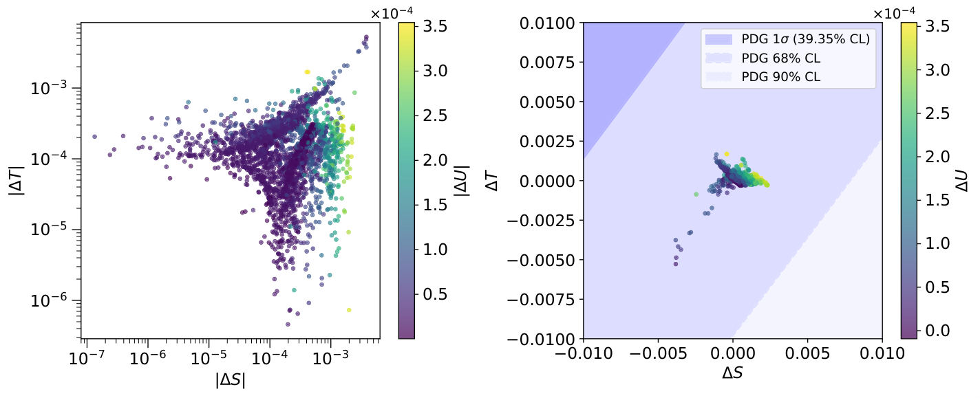
Refer to caption
Figure 12: Scanned results of the oblique parameters. The left panel takes the absolute values of the SS and TT parameters and express them in logarithmic scale. The right panel displays them on a linear scale alongside the experimental bounds.

The oblique parameters are less suppressed compared to the highly suppressed flavor observables. We investigated the source of this relative enhancement and found the SM Higgs mass to be the main driving factor. As discussed in Section IV.3, the oblique parameters are determined by the difference between the BSM and SM contributions. In the BSM contribution, the SM-like Higgs mass mh1m_{h_{1}} is scanned within its 5​σ5\sigma allowed range, and we confirmed that the dominant contribution arises from the difference between the SM-like Higgs and SM Higgs contributions. Ohter new physics contributions were also examined but found to be relatively small in comparison. As a result, the oblique parameters are the most accessible to near-future experiments, as they are quite sensitive to deviations in the SM Higgs mass. Next, we discuss lepton flavor universality, whose experimental bounds are strongly constrained as shown in Table 5, and the result is given in Figure 13.

Figure 13: Scanned results of the lepton flavor universality. The dashed line with ”SM” represents the SM prediction given in Table 5. The left panel shows all scanned points alongside the experimental bounds at 3​σ3\sigma. The right panel provides a zoomed-in view.

Since the experimental measurement of H→e+​e−H\rightarrow e^{+}e^{-} is unavailable due to the highly suppressed branching ratio from the light electron mass, we focus on the lepton flavor universality between the muon and tau. All scanned points are extremely well aligned with the SM prediction, falling within 2​σ2\sigma of the experimental bounds. This indicates that the one-loop corrections are well under control, confirming that our scan does not violate the well-established precision constraints on the ZZ and HH bosons. A further notable feature of these results is the IR contribution to the H→ℓ+​ℓ−H\rightarrow\ell^{+}\ell^{-} decays. For H→τ+​τ−H\rightarrow\tau^{+}\tau^{-}, the IR contribution is smaller by roughly one to two orders of magnitude than the sum of vertex correction and counter-term contributions. For H→μ+​μ−H\rightarrow\mu^{+}\mu^{-}, the IR contribution is smaller by roughly one order of magnitude compared to the summed contribution. For H→e+​e−H\rightarrow e^{+}e^{-}, the IR contribution is of comparable magnitude to the summed contribution. These results confirm that for heavier leptons, the IR contributions remain relatively small, whereas for lighter leptons, they become as significant as the other contributions combined.

Figure 14: Scanned results of H→InvisibleH\rightarrow\operatorname{Invisible} versus Z→InvisibleZ\rightarrow\operatorname{Invisible}. In both panels, the dashed line denotes the SM prediction for the Z→InvisibleZ\rightarrow\operatorname{Invisible} branching ratio given in Table 5. The left panel is based on the world avergae experimental bound, whereas the right panel is based on the recent ATLAS experimental bound 4

.

The last observable we discuss is the Z→InvisibleZ\rightarrow\operatorname{Invisible} decay, with the scanned results shown in Figure 14. We confirm that most of the numerical points are consistent with the world-average experimental bound at the 3​σ3\sigma level. We find that the NP contribution to the Z→InvisibleZ\rightarrow\operatorname{Invisible} decay is mainly driven by the diagonal contributions, giving rise to a numerical enhancement of 0.00040.0004, whereas the off-diagonal contributions remain relatively suppressed, of order 𝒪⁡(10−12)\mathcal{O}\left(10^{-12}\right). We also investigated the points that deviate significantly from the world-average bound, and found that these deviations arise from a numerically unstable region in which the mass of the CP-even or CP-odd scalar is nearly degenerated with that of the lightest right-handed neutrino χ1\chi_{1}, in the range 100−600​GeV100-600\operatorname{GeV}. The recent Z→InvisibleZ\rightarrow\operatorname{Invisible} measurement reported by the ATLAS collaboration features a broader 1​σ1\sigma uncertainty 4

Γ⁡(Z→Invisible)=506±2​(stat.)±12​(syst.)​MeV,\Gamma\left(Z\rightarrow\operatorname{Invisible}\right)=506\pm 2(\operatorname{stat.})\pm 12(\operatorname{syst.})\operatorname{MeV}, (51)

corresponding to BR⁡(Z→Invisible)=0.202765±0.004875\operatorname{BR}\left(Z\rightarrow\operatorname{Invisible}\right)=0.202765\pm 0.004875 using the experimental ZZ boson decay width ΓZ=2.4955​GeV\Gamma_{Z}=2.4955\operatorname{GeV} from PDG 81. This result is favored by our numerical findings at the 3​σ3\sigma level.

VI Conclusion

The SM has explained many phenomena with remarkable precision, yet several key observations remain unexplained within its framework - most notably experimentally measured nonzero neutrino masses and the existence of DM. Additionally, the SM quartic coupling constant turns negative at high energies around 109​GeV10^{9}\operatorname{GeV}, signaling an instability of the electroweak vacuum. To address these limitations, we extend the original scotogenic model by introducing an additional complex singlet scalar and a U​(1)′U(1)^{\prime} global symmetry. Within this BSM framework, we discuss the diagonalization of the flavor and scalar sectors, the one-loop neutrino mass generation mechanism for both normal and inverted hierarchies along with the relevant experimental bounds, and potential DM candidates together with their relic density constraints, further refined by incorporating EW corrections.

We investigate all constraints arising from the extended scalar sector, namely the BFB conditions, vacuum stability conditions, and perturbativity bounds induced by RG running of each parameter. For the BFB conditions, we derive both necessary and sufficient conditions by requiring V→∞V\rightarrow\infty for all possible field directions in the large field limit. For vacuum stability, we briefly discuss that the SM vacuum is considered metastable within the current experimental uncertainties on the top quark mass and the strong coupling constant αS\alpha_{S}. To identify regions of parameter space with a stable vacuum, we employ the public tool Vevacious. Finally, we investigate the RG-induced perturbativity bounds. We first motivate their necessary: perturbativity must be preserved over the entire energy range from the initial NP scale to the Planck scale, and RG-induced bounds typically place strong constraints on the couplings, making it essential to impose an upper threshold before the theory enters a Landau pole or non-perturbative regime. With this motivation, we confirm that the coupling constant gXg_{X} and quartic coupling constant λi\lambda_{i} with i=1,⋯,8i=1,\cdots,8 must each remain below 0.20.2, as determined by RG evolution of the parameters in both the SM and the present BSM model.

We next discuss several flavor and precision observables. Since this BSM model modifies the vacuum structure of the SM, accounting solely for NP contributions from NP particles is generally insufficient. Instead, we separately compute each observable in both the SM and BSM models, and take their difference as the net NP contribution. To ensure a UV-finite result, we perform a full renormalization in both models, employing the on-shell (OS) scheme in the Feynman t’Hooft gauge (ξ=1)(\xi=1), as well as the alternative tadpole scheme. For the muon g−2g-2 and the radiative decays ℓα→ℓβ​γ\ell_{\alpha}\rightarrow\ell_{\beta}\gamma, we first briefly review the current status of the Δ​aμ\Delta a_{\mu} tension, and show that both observables can be expressed in terms of the dipole operator coefficient cRc_{R}, subject to the latest experimental bounds. We then discuss the ℓα→3​ℓβ\ell_{\alpha}\rightarrow 3\ell_{\beta} decays and the μ→e\mu\rightarrow e conversion rate, presenting their analytic expressions alongside the corresponding experimental bounds. Next, we discuss the precision observables, namely the oblique parameters and the decays Z→ℓ¯α​ℓβZ\rightarrow\overline{\ell}_{\alpha}\ell_{\beta}, Z→InvisibleZ\rightarrow\operatorname{Invisible}, H→ℓ¯α​ℓβH\rightarrow\overline{\ell}_{\alpha}\ell_{\beta} and H→InvisibleH\rightarrow\operatorname{Invisible}, providing analytic expressions and experimental bounds for each. For the H→ℓ¯α​ℓβH\rightarrow\overline{\ell}_{\alpha}\ell_{\beta} decay in particular, we explicitly examine the IR structure and its cancellation via the Bremsstrahlung effects.

Finally, we perform a numerical scan. We first discuss the scanned neutrino mass spectra for both normal and inverted hierarchies. For the normal hierarchy, the sum of active neutrino masses ranges from 5.8698×10−115.8698\times 10^{-11} to 9.9913×10⁻¹¹​GeV9.9913\times 10^{-11}\operatorname{GeV}, whereas for the inverted hierarchy it ranges from 9.9453×10−119.9453\times 10^{-11} to 1.0000×10⁻¹¹​GeV1.0000\times 10^{-11}\operatorname{GeV}. The scanned inverted hierarchy spectrum would be ruled out by the recent DESI BAO result, ∑i=13mνi<6.42×10⁻¹¹​GeV\sum_{i=1}^{3}m_{\nu_{i}}<6.42\times 10^{-11}\operatorname{GeV}, if the result is confirmed by other experiments. Furthermore, the same bound excludes a large portion of the normal hierarchy parameter space as well, leaving only a small viable region.
We next discuss the potential DM candidates, their relic densities, and their spin-independent proton cross sections. We find that the CP-even scalar ηR\eta_{R} is consistently slightly heavier than the CP-odd scalar ηI\eta_{I}, leaving two viable DM candidates: ηI\eta_{I} and χ1\chi_{1}. The fermionic DM candidate χ1\chi_{1} has mass ranging from 120−350​GeV120-350\operatorname{GeV}, while the CP-odd scalar candidate ηI\eta_{I} ranges from 350−600​GeV350-600\operatorname{GeV}. Within the allowed parameter space, the fermionic and scalar DM candidates account for approximately 29%29\% and 71%71\% of the surviving points. We further examine their mass spectra against the spin-independent proton cross sections, comparing with the current experimental sensitivity from XENON1T and the projected sensitivities from XENONnT, DARWIN, and the ν\nu-floor, finding that none of these constraints place significant restrictions on the parameter space.
We find that no region of parameter space exhibits a manifest distinction between the normal and inverted neutrino mass hierarchies. Moreover, all flavor-violating observables, including the muon g−2g-2, are suppressed by many orders of magnitude relative to their current experimental bounds. Beyond these highly suppressed flavor observables, several results call for discussion. The oblique parameters are comparatively less suppressed, and the dominant contribution is traced to the mass splitting between the SM-like Higgs mh1m_{h_{1}} and the SM Higgs mhm_{h}. Other NP contributions are also examined but foundn to be small in comparison, confirming that the oblique parameters are particularly sensitive to deviations in the SM Higgs mass. We further investigate lepton flavor universality via the ratio of Z/H→ℓ​ℓZ/H\rightarrow\ell\ell decay rates, and confirm that our numerical results are consistent with the well-established experimental bounds on leptonic ZZ and HH decays. A notable feature emerging from the leptonic decays is the IR contribution to H→ℓ¯α​ℓβH\rightarrow\overline{\ell}_{\alpha}\ell_{\beta}: while this IR contribution remains relatively small for heavier leptons, it becomes comparable in magnitude to all other contributions combined for lighter leptons.
Finally, we discuss the Z→InvisibleZ\rightarrow\operatorname{Invisible} decay. The numerical scan reveals that the NP contribution to this decay is mainly driven by the diagonal contributions, giving rise to a numerical enhancement of 0.00040.0004, which is well aligned with the world-average experimental bound at the 3​σ3\sigma level. We also investigated the points that deviate significantly from the world average, finding that they originate from a numerically unstable region in which the mass of the CP-even or CP-odd scalar is nearly degenerate with that of the lightest RH neutrino χ1\chi_{1}, in the range 100−600​GeV100-600\operatorname{GeV}. We further compared our results with the recent ATLAS measurement of the decay, finding that our numerical predictions are favored at the 3​σ3\sigma level.

Acknowledgements

HL and SKK are supported by the National Research Foundation of Korea under Grant NRF-2023R1A2C100609111.

Appendix A Casas-Ibarra parameterization

The neutrino Yukawa coupling constant gXg_{X} encodes the neutrino oscillation data. They can be expressed using the Casas-Ibarra parameterization 39:

gX=UL†DL−1/2URDν1/2UPMNSTg_{X}=U_{L}^{\dagger}D_{L}^{-1/2}U_{R}D_{\nu}^{1/2}U_{\operatorname{PMNS}}^{T} (52)

where ULU_{L} and DLD_{L} are the unitary mixing matrix and the diagonalized mass matrix of the one-loop matrix MLM_{L} given in Equation 10, respectively:

DL=ULT​ML​UL,D_{L}=U_{L}^{T}M_{L}U_{L}, (53)

and DνD_{\nu} is the diagonalized mass matrix of MνM_{\nu} given in Equation 9 and UPMNSU_{\operatorname{PMNS}} is the unitary Pontecorvo-Maki-Nakagawa-Sakata mixing matrix. Furthermore, the parameters entering MLM_{L} and MνM_{\nu} do not uniquely determine the coupling matrix gXg_{X} 19. The remaining degrees of freedom are therefore encoded in the matrix URU_{R}, which can be parameterized as:

UR=UR,23​UR,13​UR,12=(1000cR,23sR,230−sR,23cR2​3)​(cR,130sR,13010−sR,130cR,13)​(cR,12sR,120−sR,12cR,120001)U_{R}=U_{R,23}U_{R,13}U_{R,12}=\begin{pmatrix}1&0&0\\ 0&c_{R,23}&s_{R,23}\\ 0&-s_{R,23}&c_{R_{2}3}\end{pmatrix}\begin{pmatrix}c_{R,13}&0&s_{R,13}\\ 0&1&0\\ -s_{R,13}&0&c_{R,13}\end{pmatrix}\begin{pmatrix}c_{R,12}&s_{R,12}&0\\ -s_{R,12}&c_{R,12}&0\\ 0&0&1\end{pmatrix} (54)

where cR,i​j=cos⁡θi​jc_{R,ij}=\cos\theta_{ij} with complex angle θi​j\theta_{ij} and sR,i​j=1−cR,i​j2s_{R,ij}=\sqrt{1-c_{R,ij}^{2}}.

Appendix B Self-energies

In this Section, we collect all the self-energies (SEs) used to derive the analytic expressions for the observables.

B.1 Photon self-energy

The diagrams contributing to the photon SE in this work are seen in Figure 15:

Figure 15: Feynman diagrams contributing to the photon SE in the scotogenic model. For the sixth diagram, an equivalent diagram with reversed charge flow is included. The charged Higgs H+H^{+} contributions are absent in the SM photon SE.

The counter-term for the photon self-energy in the scotogenic model is given in Equation 55:

δ​ZA​A=−∂ΣTA​A​(p2)∂p2|p2=0\displaystyle\delta Z_{AA}=-\left.\frac{\partial\Sigma_{T}^{AA}\left(p^{2}\right)}{\partial p^{2}}\right|_{p^{2}=0}
=e2​(sw2−1)144​cw2​(D−1)​π2[\displaystyle=\frac{e^{2}(s_{w}^{2}-1)}{144c_{w}^{2}(D-1)\pi^{2}}\Bigg[ Nc​∑i=13((2​D−4)​B0​(0,mdi2,mdi2)+8​mdi2​D​B0​(0,mdi2,mdi2))\displaystyle\phantom{{}+{}}N_{c}\sum_{i=1}^{3}\Big((2D-4)\,B_{0}(0,m_{d_{i}}^{2},m_{d_{i}}^{2})+8\,m_{d_{i}}^{2}\,DB_{0}(0,m_{d_{i}}^{2},m_{d_{i}}^{2})\Big)
+Nc∑i=13((8D−16)B0(0,mui2,mui2)+32mui2DB0(0,mui2,mui2))\displaystyle+N_{c}\sum_{i=1}^{3}\Big((8D-16)\,B_{0}(0,m_{u_{i}}^{2},m_{u_{i}}^{2})+32\,m_{u_{i}}^{2}\,DB_{0}(0,m_{u_{i}}^{2},m_{u_{i}}^{2})\Big)
+∑i=13((18D−36)B0(0,mei2,mei2)+72mei2DB0(0,mei2,mei2))\displaystyle+\sum_{i=1}^{3}\Big((18D-36)\,B_{0}(0,m_{e_{i}}^{2},m_{e_{i}}^{2})+72\,m_{e_{i}}^{2}\,DB_{0}(0,m_{e_{i}}^{2},m_{e_{i}}^{2})\Big)
+(27−27​D)​B0​(0,MW2,MW2)+(36−36​D)​MW2​D​B0​(0,MW2,MW2)\displaystyle+(27-27D)\,B_{0}(0,M_{W}^{2},M_{W}^{2})+(36-36D)\,M_{W}^{2}\,DB_{0}(0,M_{W}^{2},M_{W}^{2})
+9B0(0,MH±2,MH±2)−36MH±2DB0(0,MH±2,MH±2)]\displaystyle+9\,B_{0}(0,M_{H^{\pm}}^{2},M_{H^{\pm}}^{2})-36\,M_{H^{\pm}}^{2}\,DB_{0}(0,M_{H^{\pm}}^{2},M_{H^{\pm}}^{2})\Bigg] (55)

where the B0B_{0} and D​B0DB_{0} are the Passarino-Veltman functions. The charged Higgs contributions are absent in the SM photon SE.

B.2 Photon-ZZ self-energy

The diagrams contributing to the photon-ZZ SE in this work are seen in Figure 16:

Figure 16: Feynman diagrams contributing to the photon SE in the scotogenic model. For the sixth diagram, an equivalent diagram with reversed charge flow is included. The charged Higgs H+H^{+} contributions are absent in the SM photon SE.

The counter-terms for the photon-ZZ self-energy in the scotogenic model is given in Equation 56:

δ​ZZ​A\displaystyle\delta Z_{ZA} =2MZ2​ΣTA​Z​(0)=−e2​cw​B0​(0,MW2,MW2)4​π2​sw,\displaystyle=\frac{2}{M_{Z}^{2}}\Sigma_{T}^{AZ}\left(0\right)=-\frac{e^{2}c_{w}\operatorname{B}_{0}\left(0,M_{W}^{2},M_{W}^{2}\right)}{4\pi^{2}s_{w}},
δ​ZA​Z\displaystyle\delta Z_{AZ} =−2ReΣTA​Z​(MZ2)MZ2=e2144​cw​(1−D)​MZ2​π2​sw[\displaystyle=-2\operatorname{Re}\frac{\Sigma_{T}^{AZ}\left(M_{Z}^{2}\right)}{M_{Z}^{2}}=\frac{e^{2}}{144\,c_{w}(1-D)M_{Z}^{2}\pi^{2}s_{w}}\Bigg[
+36​MH±2​(1−2​sw2)​B0​(0,MH±2,MH±2)\displaystyle+36M_{H^{\pm}}^{2}\left(1-2s_{w}^{2}\right)B_{0}\!\left(0,M_{H^{\pm}}^{2},M_{H^{\pm}}^{2}\right)
−36​MW2​(3−2​D+2​(D−1)​sw2)​B0​(0,MW2,MW2)\displaystyle-36M_{W}^{2}\left(3-2D+2(D-1)s_{w}^{2}\right)B_{0}\!\left(0,M_{W}^{2},M_{W}^{2}\right)
+9​(4​MH±2−MZ2)​(2​sw2−1)​B0​(MZ2,MH±2,MH±2)\displaystyle+9\left(4M_{H^{\pm}}^{2}-M_{Z}^{2}\right)\left(2s_{w}^{2}-1\right)B_{0}\!\left(M_{Z}^{2},M_{H^{\pm}}^{2},M_{H^{\pm}}^{2}\right)
+9(4MW2(4−3D+3(D−1)sw2)\displaystyle+9\Big(4M_{W}^{2}\left(4-3D+3(D-1)s_{w}^{2}\right)
+MZ2(5−6D+6(D−1)sw2)−(D−1)e2v2)B0(MZ2,MW2,MW2)\displaystyle\qquad+M_{Z}^{2}\left(5-6D+6(D-1)s_{w}^{2}\right)-(D-1)e^{2}v^{2}\Big)B_{0}\!\left(M_{Z}^{2},M_{W}^{2},M_{W}^{2}\right)
+36(4sw2−1)∑i=13mei2B0(0,mei2,mei2)\displaystyle\qquad+36\left(4s_{w}^{2}-1\right)\sum_{i=1}^{3}m_{e_{i}}^{2}\,B_{0}\!\left(0,m_{e_{i}}^{2},m_{e_{i}}^{2}\right)
−9(4sw2−1)∑i=13((D−2)MZ2+4mei2)B0(MZ2,mei2,mei2)\displaystyle-9\left(4s_{w}^{2}-1\right)\sum_{i=1}^{3}\left((D-2)M_{Z}^{2}+4m_{e_{i}}^{2}\right)B_{0}\!\left(M_{Z}^{2},m_{e_{i}}^{2},m_{e_{i}}^{2}\right)
+4(4sw2−3)Nc∑i=13mdi2B0(0,mdi2,mdi2)\displaystyle+4\left(4s_{w}^{2}-3\right)N_{c}\sum_{i=1}^{3}m_{d_{i}}^{2}\,B_{0}\!\left(0,m_{d_{i}}^{2},m_{d_{i}}^{2}\right)
+8(8sw2−3)Nc∑i=13mui2B0(0,mui2,mui2)\displaystyle+8\left(8s_{w}^{2}-3\right)N_{c}\sum_{i=1}^{3}m_{u_{i}}^{2}\,B_{0}\!\left(0,m_{u_{i}}^{2},m_{u_{i}}^{2}\right)
−(4sw2−3)Nc∑i=13((D−2)MZ2+4mdi2)B0(MZ2,mdi2,mdi2)\displaystyle-\left(4s_{w}^{2}-3\right)N_{c}\sum_{i=1}^{3}\left((D-2)M_{Z}^{2}+4m_{d_{i}}^{2}\right)B_{0}\!\left(M_{Z}^{2},m_{d_{i}}^{2},m_{d_{i}}^{2}\right)
−2(8sw2−3)Nc∑i=13((D−2)MZ2+4mui2)B0(MZ2,mui2,mui2)]\displaystyle-2\left(8s_{w}^{2}-3\right)N_{c}\sum_{i=1}^{3}\left((D-2)M_{Z}^{2}+4m_{u_{i}}^{2}\right)B_{0}\!\left(M_{Z}^{2},m_{u_{i}}^{2},m_{u_{i}}^{2}\right)\Bigg] (56)

where the charged Higgs contributions are absent in the SM photon-ZZ SE.

B.3 ZZ self-energy

From ZZ SE, the tadpole contributions start to appear. Therefore, we split them for better visibility. The diagrams contributing to the ZZ tadpoles and ZZ SEs are seen in Figures 17 and 18.

Figure 17: Feynman diagrams contributing to the ZZ boson tadpole in the scotogenic model, where i,j=1,2i,j=1,2. In the SM limit, hih_{i} and aia_{i} reduce to the SM Higgs boson hh and the would-be Goldstone boson aa of the ZZ boson, respectively, while the contributions involving the χ,ηR,I\chi,\eta_{R,I} and H+H^{+} fields are absent.
Figure 18: Feynman diagrams contributing to the ZZ boson tadpole in the scotogenic model, where i,j=1,2i,j=1,2. In the SM limit, hih_{i} and aia_{i} reduce to the SM Higgs boson hh and the would-be Goldstone boson aa of the ZZ boson, respectively, while the contributions involving the χ\chi and H+H^{+} fields are absent.

With the explicit tadpole contributions, the SE in the alternative tadpole scheme is redefined as 73:

ΣTZ​Z​(p2)≡ΣTZ​Z​(p2)+ΣTZ​Z,Tad​(p2)\Sigma_{T}^{ZZ}\left(p^{2}\right)\equiv\Sigma_{T}^{ZZ}\left(p^{2}\right)+\Sigma_{T}^{ZZ,\operatorname{Tad}}\left(p^{2}\right) (57)

This definition applies to all other SEs which feature explicit tadpole contributions. Then, the mass and field CT terms for the ZZ SE are given in Equations 58 and 59.

δ​MZ2\displaystyle\delta M_{Z}^{2} =Re⁡ΣTZ​Z​(MZ2)\displaystyle=\operatorname{Re}\Sigma_{T}^{ZZ}\left(M_{Z}^{2}\right)
=164​cw2​(−1+D)​MZ2​π2​sw2​e2​(MηR−MηI−MZ)​(MηR+MηI−MZ)\displaystyle=\frac{1}{64c_{w}^{2}(-1+D)M_{Z}^{2}\pi^{2}s_{w}^{2}}e^{2}(M_{\eta_{R}}-M_{\eta_{I}}-M_{Z})(M_{\eta_{R}}+M_{\eta_{I}}-M_{Z})
×(MηR−MηI+MZ)​(MηR+MηI+MZ)​B0​(MZ2,MηR2,MηI2)\displaystyle\times(M_{\eta_{R}}-M_{\eta_{I}}+M_{Z})(M_{\eta_{R}}+M_{\eta_{I}}+M_{Z})B_{0}\Big(M_{Z}^{2},M_{\eta_{R}}^{2},M_{\eta_{I}}^{2}\Big)
−164​cw2​(−1+D)​π2​sw2​(4​MH+−MZ2)​(e−2​e​sw2)2​B0​(MZ2,MH+2,MH+2)\displaystyle-\frac{1}{64c_{w}^{2}(-1+D)\pi^{2}s_{w}^{2}}\Big(4M_{H^{+}}-M_{Z}^{2}\Big)\Big(e-2es_{w}^{2}\Big)^{2}\ B_{0}\Big(M_{Z}^{2},M^{2}_{H^{+}},M^{2}_{H^{+}}\Big)
+164​cw2​(−1+D)​π2​sw2​e2​MZ2​(−3+4​sw2)​(−15+12​D+(20−16​D)​sw2+4​(−1+D)​sw4)\displaystyle+\frac{1}{64c_{w}^{2}(-1+D)\pi^{2}s_{w}^{2}}e^{2}M_{Z}^{2}\Big(-3+4s_{w}^{2}\Big)\Big(-15+12D+(20-16D)s_{w}^{2}+4\ (-1+D)s_{w}^{4}\Big)
×B0​(MZ2,MW2,MW2)\displaystyle\times B_{0}\Big(M_{Z}^{2},M_{W}^{2},M_{W}^{2}\Big)
+164​cw2​(−1+D)​π2​sw2​3​(−2+D)​e2​MZ2​B0​(MZ2,0,0)\displaystyle+\frac{1}{64c_{w}^{2}(-1+D)\pi^{2}s_{w}^{2}}3(-2+D)e^{2}M_{Z}^{2}B_{0}\Big(M_{Z}^{2},0,0\Big)
+∑k=13164​cw2​(−1+D)​π2​sw2e2B0(MZ2,mek2,mek2)((−2+D)MZ2(1−4sw2+8sw4)\displaystyle+\sum_{k=1}^{3}\frac{1}{64c_{w}^{2}(-1+D)\pi^{2}s_{w}^{2}}e^{2}B_{0}\Big(M_{Z}^{2},m_{e_{k}}^{2},m_{e_{k}}^{2}\Big)\Big((-2+D)M_{Z}^{2}\Big(1-4s_{w}^{2}+8s_{w}^{4}\Big)
−2(−3+D+8sw2−16sw4)mek2)\displaystyle-2\Big(-3+D+8s_{w}^{2}-16s_{w}^{4}\Big)m_{e_{k}}^{2}\Big)
+∑k=131576​cw2​(−1+D)​π2​sw2e2NcB0(MZ2,mdk2,mdk2)((−2+D)MZ2(9−12sw2+8sw4)\displaystyle+\sum_{k=1}^{3}\frac{1}{576c_{w}^{2}(-1+D)\pi^{2}s_{w}^{2}}e^{2}N_{c}B_{0}\Big(M_{Z}^{2},m_{d_{k}}^{2},m_{d_{k}}^{2}\Big)\Big((-2+D)M_{Z}^{2}\Big(9-12s_{w}^{2}+8s_{w}^{4}\Big)
+(54−18D−48sw2+32sw4)mdk2)\displaystyle+\Big(54-18D-48s_{w}^{2}+32s_{w}^{4}\Big)m_{d_{k}}^{2}\Big)
+∑k=131576​cw2​(−1+D)​π2​sw2e2NcB0(MZ2,muk2,muk2)((−2+D)MZ2(9−24sw2+32sw4)\displaystyle+\sum_{k=1}^{3}\frac{1}{576c_{w}^{2}(-1+D)\pi^{2}s_{w}^{2}}e^{2}N_{c}B_{0}\Big(M_{Z}^{2},m_{u_{k}}^{2},m_{u_{k}}^{2}\Big)\Big((-2+D)M_{Z}^{2}\Big(9-24s_{w}^{2}+32s_{w}^{4}\Big)
−2(−27+9D+48sw2−64sw4)muk2)\displaystyle-2\Big(-27+9D+48s_{w}^{2}-64s_{w}^{4}\Big)m_{u_{k}}^{2}\Big)
+∑i=12132​cw2​(−2+D)​(−1+D)​MZ2​π2​sw2−e2B0(0,Mhi2,Mhi2)Mhi2(−(−1+D)MZ2+Mhi2)Ui​1H,2\displaystyle+\sum_{i=1}^{2}\frac{1}{32c_{w}^{2}(-2+D)(-1+D)M_{Z}^{2}\pi^{2}s_{w}^{2}}-e^{2}B_{0}\Big(0,M_{h_{i}}^{2},M_{h_{i}}^{2}\Big)M_{h_{i}}^{2}\Big(-(-1+D)M_{Z}^{2}+M_{h_{i}}^{2}\Big)U^{H,2}_{i1}
+∑i=12164​cw2​(−1+D)​MZ2​π2​sw2e2B0(MZ2,MZ2,Mhi2)(4(−1+D)MZ4−4MZ2Mhi2+Mhi4)Ui​1H,2\displaystyle+\sum_{i=1}^{2}\frac{1}{64c_{w}^{2}(-1+D)M_{Z}^{2}\pi^{2}s_{w}^{2}}e^{2}B_{0}\Big(M_{Z}^{2},M_{Z}^{2},M_{h_{i}}^{2}\Big)\Big(4(-1+D)M_{Z}^{4}-4M_{Z}^{2}M_{h_{i}}^{2}+M_{h_{i}}^{4}\Big)U^{H,2}_{i1}
+∑k=13116​cw2​(−2+D)​(−1+D)​π2​sw2​Mhi2e2B0(0,mek2,mek2)mek2(−(−2+D)(1−4sw2+8sw4)Mhi2\displaystyle+\sum_{k=1}^{3}\frac{1}{16c_{w}^{2}(-2+D)(-1+D)\pi^{2}s_{w}^{2}M_{h_{i}}^{2}}e^{2}B_{0}\Big(0,m_{e_{k}}^{2},m_{e_{k}}^{2}\Big)m_{e_{k}}^{2}\Big(-(-2+D)\Big(1-4s_{w}^{2}+8s_{w}^{4}\Big)M_{h_{i}}^{2}
+∑i=124(−1+D)mek2Ui​1H,2)\displaystyle+\sum_{i=1}^{2}4(-1+D)m_{e_{k}}^{2}U^{H,2}_{i1}\Big)
+∑k=131144​cw2​(−2+D)​(−1+D)​π2​sw2​Mhi2e2NcB0(0,muk2,muk2)muk2(−(−2+D)\displaystyle+\sum_{k=1}^{3}\frac{1}{144c_{w}^{2}(-2+D)(-1+D)\pi^{2}s_{w}^{2}M_{h_{i}}^{2}}e^{2}N_{c}B_{0}\Big(0,m_{u_{k}}^{2},m_{u_{k}}^{2}\Big)m_{u_{k}}^{2}\Big(-(-2+D)
×(9−24sw2+32sw4)Mhi2+∑i=1236(−1+D)muk2Ui​1H,2)\displaystyle\times\Big(9-24s_{w}^{2}+32s_{w}^{4}\Big)M_{h_{i}}^{2}+\sum_{i=1}^{2}36(-1+D)m_{u_{k}}^{2}U^{H,2}_{i1}\Big)
+∑k=131144​cw2​(−2+D)​(−1+D)​π2​sw2​Mhi2e2NcB0(0,mdk2,mdk2)mdk2(−(−2+D)\displaystyle+\sum_{k=1}^{3}\frac{1}{144c_{w}^{2}(-2+D)(-1+D)\pi^{2}s_{w}^{2}M_{h_{i}}^{2}}e^{2}N_{c}B_{0}\Big(0,m_{d_{k}}^{2},m_{d_{k}}^{2}\Big)m_{d_{k}}^{2}\Big(-(-2+D)
×(9−12sw2+8sw4)Mhi2+∑i=1236(−1+D)mdk2UL,k,kDUi​1H,2)\displaystyle\times\Big(9-12s_{w}^{2}+8s_{w}^{4}\Big)M_{h_{i}}^{2}+\sum_{i=1}^{2}36(-1+D)m_{d_{k}}^{2}U^{D}_{L,k,k}U^{H,2}_{i1}\Big)
+∑i=12(∑k=1314​cw​(−2+D)​π2​sw​vS​Mhi2eMZB0(0,Mχk2,Mχk2)Mχk4Ui​1HUi​2H\displaystyle+\sum_{i=1}^{2}\Big(\sum_{k=1}^{3}\frac{1}{4c_{w}(-2+D)\pi^{2}s_{w}v_{S}M_{h_{i}}^{2}}eM_{Z}B_{0}\Big(0,M_{\chi_{k}}^{2},M_{\chi_{k}}^{2}\Big)M_{\chi_{k}}^{4}U^{H}_{i1}U^{H}_{i2}
−∑i=12132​cw​(−2+D)​π2​sw​Mhi2MA2MZB0(0,MA2,MA2)Ui​1H(4cwλ7MZswUi​1H+eλ6vSUi​2H)\displaystyle-\sum_{i=1}^{2}\frac{1}{32c_{w}(-2+D)\pi^{2}s_{w}M_{h_{i}}^{2}}M_{A}^{2}M_{Z}B_{0}\Big(0,M_{A}^{2},M_{A}^{2}\Big)U^{H}_{i1}(4c_{w}\lambda_{7}M_{Z}s_{w}U^{H}_{i1}+e\lambda_{6}v_{S}U^{H}_{i2})
+132​cw2​(−2+D)​(−1+D)​MZ2​π2​sw2​Mhi2MηI2B0(0,MηI2,MηI2)(e2MηR2Mhi2−e2MηI2Mhi2\displaystyle+\frac{1}{32c_{w}^{2}(-2+D)(-1+D)M_{Z}^{2}\pi^{2}s_{w}^{2}M_{h_{i}}^{2}}M_{\eta_{I}}^{2}B_{0}\Big(0,M_{\eta_{I}}^{2},M_{\eta_{I}}^{2}\Big)\Big(e^{2}M_{\eta_{R}}^{2}M_{h_{i}}^{2}-e^{2}M_{\eta_{I}}^{2}M_{h_{i}}^{2}
−2e2MZ2Mhi2+De2MZ2Mhi2+∑i=12−2(−1+D)(2λ3+2λ4−λ5)MZ4sw2Ui​1H,2\displaystyle-2e^{2}M_{Z}^{2}M_{h_{i}}^{2}+De^{2}M_{Z}^{2}M_{h_{i}}^{2}+\sum_{i=1}^{2}-2(-1+D)(2\lambda_{3}+2\lambda_{4}-\lambda_{5})M_{Z}^{4}s_{w}^{2}U^{H,2}_{i1}
+∑i=122(−1+D)(2λ3+2λ4−λ5)MZ4sw4Ui​1H,2+∑i=12−2cw(−1+D)eλ8MZ3swvSUi​1HUi​2H)\displaystyle+\sum_{i=1}^{2}2(-1+D)(2\lambda_{3}+2\lambda_{4}-\lambda_{5})M_{Z}^{4}s_{w}^{4}U^{H,2}_{i1}+\sum_{i=1}^{2}-2c_{w}(-1+D)e\lambda_{8}M_{Z}^{3}s_{w}v_{S}U^{H}_{i1}U^{H}_{i2}\Big)
+132​cw2​(−2+D)​(−1+D)​MZ2​π2​sw2​Mhi2−MηR2B0(0,MηR2,MηR2)(e2MηR2Mhi2−e2MηI2Mhi2\displaystyle+\frac{1}{32c_{w}^{2}(-2+D)(-1+D)M_{Z}^{2}\pi^{2}s_{w}^{2}M_{h_{i}}^{2}}-M_{\eta_{R}}^{2}B_{0}\Big(0,M_{\eta_{R}}^{2},M_{\eta_{R}}^{2}\Big)\Big(e^{2}M_{\eta_{R}}^{2}M_{h_{i}}^{2}-e^{2}M_{\eta_{I}}^{2}M_{h_{i}}^{2}
+2​e2​MZ2​Mhi2−D​e2​MZ2​Mhi2+∑i=122​(−1+D)​(2​λ3+2​λ4+λ5)​MZ4​sw2​Ui​1H,2\displaystyle+2e^{2}M_{Z}^{2}M_{h_{i}}^{2}-De^{2}M_{Z}^{2}M_{h_{i}}^{2}+\sum_{i=1}^{2}2(-1+D)(2\lambda_{3}+2\lambda_{4}+\lambda_{5})M_{Z}^{4}s_{w}^{2}U^{H,2}_{i1}
+∑i=12−2(−1+D)(2λ3+2λ4+λ5)MZ4sw4Ui​1H,2+∑i=122cw(−1+D)eλ8MZ3swvSUi​1HUi​2H)\displaystyle+\sum_{i=1}^{2}-2(-1+D)(2\lambda_{3}+2\lambda_{4}+\lambda_{5})M_{Z}^{4}s_{w}^{4}U^{H,2}_{i1}+\sum_{i=1}^{2}2c_{w}(-1+D)e\lambda_{8}M_{Z}^{3}s_{w}v_{S}U^{H}_{i1}U^{H}_{i2}\Big)
+116​cw2​(−2+D)​(−1+D)​π2​sw2​Mhi2MH+B0(0,MH+,MH+)((−2+D)e2(1−2sw2)2Mhi2\displaystyle+\frac{1}{16c_{w}^{2}(-2+D)(-1+D)\pi^{2}s_{w}^{2}M_{h_{i}}^{2}}M_{H^{+}}B_{0}\Big(0,M_{H^{+}},M_{H^{+}}\Big)\Big((-2+D)e^{2}\Big(1-2s_{w}^{2}\Big)^{2}M_{h_{i}}^{2}
+∑i=122(−1+D)MZswUi​1H(2λ3MZsw(−1+sw2)Ui​1H−cweλ8vSUi​2H))\displaystyle+\sum_{i=1}^{2}2(-1+D)M_{Z}s_{w}U^{H}_{i1}\Big(2\lambda_{3}M_{Z}s_{w}\Big(-1+s_{w}^{2}\Big)U^{H}_{i1}-c_{w}e\lambda_{8}v_{S}U^{H}_{i2}\Big)\Big)
+132​cw2​(−2+D)​(−1+D)​π2​sw2​Mhi2−B0(0,MZ2,MZ2)(e2MZ2Mhi2(1−D+∑i=122Ui​1H,2)\displaystyle+\frac{1}{32c_{w}^{2}(-2+D)(-1+D)\pi^{2}s_{w}^{2}M_{h_{i}}^{2}}-B_{0}\Big(0,M_{Z}^{2},M_{Z}^{2}\Big)\Big(e^{2}M_{Z}^{2}M_{h_{i}}^{2}\Big(1-D+\sum_{i=1}^{2}2U^{H,2}_{i1}\Big)
+∑i=12−e2Mhi4Ui​1H,2+∑i=122(−1+D)MZ3Ui​1H(MZ((−1+D)e2+λ1sw2−λ1sw4)Ui​1H+cweλ7swvSUi​2H))\displaystyle+\sum_{i=1}^{2}-e^{2}M_{h_{i}}^{4}U^{H,2}_{i1}+\sum_{i=1}^{2}2(-1+D)M_{Z}^{3}U^{H}_{i1}\Big(M_{Z}\Big((-1+D)e^{2}+\lambda_{1}s_{w}^{2}-\lambda_{1}s_{w}^{4}\Big)U^{H}_{i1}+c_{w}e\lambda_{7}s_{w}v_{S}U^{H}_{i2}\Big)\Big)
+116​(−2+D)​(−1+D)​π2​sw2​Mhi2MZ2B0(0,MW2,MW2)(e2(14−15D+4D2\displaystyle+\frac{1}{16(-2+D)(-1+D)\pi^{2}s_{w}^{2}M_{h_{i}}^{2}}M_{Z}^{2}B_{0}\Big(0,M_{W}^{2},M_{W}^{2}\Big)\Big(e^{2}\Big(14-15D+4D^{2}
−4(6−7D+2D2)sw2+4(2−3D+D2)sw4)Mhi2\displaystyle-4\Big(6-7D+2D^{2}\Big)s_{w}^{2}+4\Big(2-3D+D^{2}\Big)s_{w}^{4}\Big)M_{h_{i}}^{2}
+∑i=122(−1+D)MZUi​1H(MZ(−1+sw2)((−1+D)e2+λ1sw2)Ui​1H−cweλ7swvSUi​2H))\displaystyle+\sum_{i=1}^{2}2(-1+D)M_{Z}U^{H}_{i1}\Big(M_{Z}\Big(-1+s_{w}^{2}\Big)\Big((-1+D)e^{2}+\lambda_{1}s_{w}^{2}\Big)U^{H}_{i1}-c_{w}e\lambda_{7}s_{w}v_{S}U^{H}_{i2}\Big)\Big)
+∑i=12(∑j=12132​cw​(−2+D)​π2​sw​Mhi2−MZB0(0,Mhj2,Mhj2)Mhj2Ui​1H\displaystyle+\sum_{i=1}^{2}\Big(\sum_{j=1}^{2}\frac{1}{32c_{w}(-2+D)\pi^{2}s_{w}M_{h_{i}}^{2}}-M_{Z}B_{0}\Big(0,M_{h_{j}}^{2},M_{h_{j}}^{2}\Big)M_{h_{j}}^{2}U^{H}_{i1}
×(Ui​2H(2eλ7vSUj​1H,2+8cwλ7MZswUj​1HUj​2H+3eλ6vSUj​2H,2)\displaystyle\times\Big(U^{H}_{i2}\Big(2e\lambda_{7}v_{S}U^{H,2}_{j1}+8c_{w}\lambda_{7}M_{Z}s_{w}U^{H}_{j1}U^{H}_{j2}+3e\lambda_{6}v_{S}U^{H,2}_{j2}\Big)
+2Ui​1H(2eλ7vSUj​1HUj​2H+cwMZsw(3λ1Uj​1H,2+2λ7Uj​2H,2)))\displaystyle+2U^{H}_{i1}\Big(2e\lambda_{7}v_{S}U^{H}_{j1}U^{H}_{j2}+c_{w}M_{Z}s_{w}\Big(3\lambda_{1}U^{H,2}_{j1}+2\lambda_{7}U^{H,2}_{j2}\Big)\Big)\Big) (58)
δ​ZZ​Z\displaystyle\delta Z_{ZZ} =−Re⁡∂ΣTZ​Z​(p2)∂p2|p2=MZ2\displaystyle=-\operatorname{Re}\left.\frac{\partial\Sigma_{T}^{ZZ}\left(p^{2}\right)}{\partial p^{2}}\right|_{p^{2}=M_{Z}^{2}}
=132​cw2​(−2+D)​(−1+D)​MZ4​π2​sw2​e2​MηR2​(−MηR2+MηI2)​B0​(0,MηR2,MηR2)\displaystyle=\frac{1}{32c_{w}^{2}(-2+D)(-1+D)M_{Z}^{4}\pi^{2}s_{w}^{2}}e^{2}M_{\eta_{R}}^{2}\Big(-M_{\eta_{R}}^{2}+M_{\eta_{I}}^{2}\Big)B_{0}\Big(0,M_{\eta_{R}}^{2},M_{\eta_{R}}^{2}\Big)
+132​cw2​(−2+D)​(−1+D)​MZ4​π2​sw2​e2​MηI2​(MηR2−MηI2)​B0​(0,MηI2,MηI2)\displaystyle+\frac{1}{32c_{w}^{2}(-2+D)(-1+D)M_{Z}^{4}\pi^{2}s_{w}^{2}}e^{2}M_{\eta_{I}}^{2}\Big(M_{\eta_{R}}^{2}-M_{\eta_{I}}^{2}\Big)B_{0}\Big(0,M_{\eta_{I}}^{2},M_{\eta_{I}}^{2}\Big)
+164​cw2​(−1+D)​MZ4​π2​sw2​e2​(MηR4−2​MηR2​MηI2+MηI4−MZ4)​B0​(MZ2,MηR2,MηI2)\displaystyle+\frac{1}{64c_{w}^{2}(-1+D)M_{Z}^{4}\pi^{2}s_{w}^{2}}e^{2}\Big(M_{\eta_{R}}^{4}-2M_{\eta_{R}}^{2}M_{\eta_{I}}^{2}+M_{\eta_{I}}^{4}-M_{Z}^{4}\Big)B_{0}\Big(M_{Z}^{2},M_{\eta_{R}}^{2},M_{\eta_{I}}^{2}\Big)
+164​cw2​(−1+D)​π2​sw2−(e−2​e​sw2)2​B0​(MZ2,MH+2,MH+2)\displaystyle+\frac{1}{64c_{w}^{2}(-1+D)\pi^{2}s_{w}^{2}}-\Big(e-2es_{w}^{2}\Big)^{2}B_{0}\Big(M_{Z}^{2},M^{2}_{H^{+}},M^{2}_{H^{+}}\Big)
+164​cw2​(−1+D)​π2​sw2​e2​(3​cw4​(−3+4​D)+2​cw2​sw2−sw4)​B0​(MZ2,MW2,MW2)\displaystyle+\frac{1}{64c_{w}^{2}(-1+D)\pi^{2}s_{w}^{2}}e^{2}\Big(3c_{w}^{4}(-3+4D)+2c_{w}^{2}s_{w}^{2}-s_{w}^{4}\Big)B_{0}\Big(M_{Z}^{2},M_{W}^{2},M_{W}^{2}\Big)
+164​cw2​(−1+D)​π2​sw2−3​(−2+D)​e2​B0​(MZ2,0,0)\displaystyle+\frac{1}{64c_{w}^{2}(-1+D)\pi^{2}s_{w}^{2}}-3(-2+D)e^{2}B_{0}\Big(M_{Z}^{2},0,0\Big)
+∑k=13164​cw2​(−1+D)​π2​sw2−(−2+D)e2(1−4sw2+8sw4)B0(MZ2,mek2,mek2)\displaystyle+\sum_{k=1}^{3}\frac{1}{64c_{w}^{2}(-1+D)\pi^{2}s_{w}^{2}}-(-2+D)e^{2}\Big(1-4s_{w}^{2}+8s_{w}^{4}\Big)B_{0}\Big(M_{Z}^{2},m_{e_{k}}^{2},m_{e_{k}}^{2}\Big)
+∑k=131576​cw2​(−1+D)​π2​sw2−(−2+D)e2Nc(9−12sw2+8sw4)B0(MZ2,mdk2,mdk2)\displaystyle+\sum_{k=1}^{3}\frac{1}{576c_{w}^{2}(-1+D)\pi^{2}s_{w}^{2}}-(-2+D)e^{2}N_{c}\Big(9-12s_{w}^{2}+8s_{w}^{4}\Big)B_{0}\Big(M_{Z}^{2},m_{d_{k}}^{2},m_{d_{k}}^{2}\Big)
+∑k=131576​cw2​(−1+D)​π2​sw2−(−2+D)e2Nc(9−24sw2+32sw4)B0(MZ2,muk2,muk2)\displaystyle+\sum_{k=1}^{3}\frac{1}{576c_{w}^{2}(-1+D)\pi^{2}s_{w}^{2}}-(-2+D)e^{2}N_{c}\Big(9-24s_{w}^{2}+32s_{w}^{4}\Big)B_{0}\Big(M_{Z}^{2},m_{u_{k}}^{2},m_{u_{k}}^{2}\Big)
+∑i=12132​cw2​(−2+D)​(−1+D)​MZ2​π2​sw2−e2B0(0,MZ2,MZ2)(MZ2−Mhi2)Ui​1H,2\displaystyle+\sum_{i=1}^{2}\frac{1}{32c_{w}^{2}(-2+D)(-1+D)M_{Z}^{2}\pi^{2}s_{w}^{2}}-e^{2}B_{0}\Big(0,M_{Z}^{2},M_{Z}^{2}\Big)\Big(M_{Z}^{2}-M_{h_{i}}^{2}\Big)U^{H,2}_{i1}
+∑i=12132​cw2​(−2+D)​(−1+D)​MZ4​π2​sw2e2B0(0,Mhi2,Mhi2)Mhi2(MZ2−Mhi2)Ui​1H,2\displaystyle+\sum_{i=1}^{2}\frac{1}{32c_{w}^{2}(-2+D)(-1+D)M_{Z}^{4}\pi^{2}s_{w}^{2}}e^{2}B_{0}\Big(0,M_{h_{i}}^{2},M_{h_{i}}^{2}\Big)M_{h_{i}}^{2}\Big(M_{Z}^{2}-M_{h_{i}}^{2}\Big)U^{H,2}_{i1}
+∑i=12164​cw2​(−1+D)​MZ4​π2​sw2e2B0(MZ2,MZ2,Mhi2)Mhi2(−2MZ2+Mhi2)Ui​1H,2\displaystyle+\sum_{i=1}^{2}\frac{1}{64c_{w}^{2}(-1+D)M_{Z}^{4}\pi^{2}s_{w}^{2}}e^{2}B_{0}\Big(M_{Z}^{2},M_{Z}^{2},M_{h_{i}}^{2}\Big)M_{h_{i}}^{2}\Big(-2M_{Z}^{2}+M_{h_{i}}^{2}\Big)U^{H,2}_{i1}
−1576​cw2​(−1+D)​MZ2​π2​sw2e2(−54MZ4DB0(MZ2,0,0)+27DMZ4DB0(MZ2,0,0)\displaystyle-\frac{1}{576c_{w}^{2}(-1+D)M_{Z}^{2}\pi^{2}s_{w}^{2}}e^{2}\Big(-54M_{Z}^{4}DB_{0}\Big(M_{Z}^{2},0,0\Big)+27DM_{Z}^{4}DB_{0}\Big(M_{Z}^{2},0,0\Big)
+9​(MηR4+(MηI2−MZ2)2−2​MηR2​(MηI2+MZ2))​D​B0​(MZ2,MηR2,MηI2)\displaystyle+9\Big(M_{\eta_{R}}^{4}+\Big(M_{\eta_{I}}^{2}-M_{Z}^{2}\Big)^{2}-2M_{\eta_{R}}^{2}\Big(M_{\eta_{I}}^{2}+M_{Z}^{2}\Big)\Big)DB_{0}\Big(M_{Z}^{2},M_{\eta_{R}}^{2},M_{\eta_{I}}^{2}\Big)
+9​(−4​MH++MZ2)​(MZ−2​MZ​sw2)2​D​B0​(MZ2,MH+,MH+)+405​MZ4​D​B0​(MZ2,MW2,MW2)\displaystyle+9\Big(-4M_{H^{+}}+M_{Z}^{2}\Big)\Big(M_{Z}-2M_{Z}s_{w}^{2}\Big)^{2}DB_{0}\Big(M_{Z}^{2},M_{H^{+}},M_{H^{+}}\Big)+405M_{Z}^{4}DB_{0}\Big(M_{Z}^{2},M_{W}^{2},M_{W}^{2}\Big)
−324​D​MZ4​D​B0​(MZ2,MW2,MW2)+144​(−1+D)​MZ4​sw6​D​B0​(MZ2,MW2,MW2)\displaystyle-324DM_{Z}^{4}DB_{0}\Big(M_{Z}^{2},M_{W}^{2},M_{W}^{2}\Big)+144(-1+D)M_{Z}^{4}s_{w}^{6}DB_{0}\Big(M_{Z}^{2},M_{W}^{2},M_{W}^{2}\Big)
+∑k=13−18MZ4NcDB0(MZ2,mdk2,mdk2)+∑k=139DMZ4NcDB0(MZ2,mdk2,mdk2)+∑k=13\displaystyle+\sum_{k=1}^{3}-18M_{Z}^{4}N_{c}DB_{0}\Big(M_{Z}^{2},m_{d_{k}}^{2},m_{d_{k}}^{2}\Big)+\sum_{k=1}^{3}9DM_{Z}^{4}N_{c}DB_{0}\Big(M_{Z}^{2},m_{d_{k}}^{2},m_{d_{k}}^{2}\Big)+\sum_{k=1}^{3}
−18​MZ4​D​B0​(MZ2,mek2,mek2)+∑k=139​D​MZ4​D​B0​(MZ2,mek2,mek2)\displaystyle-18M_{Z}^{4}DB_{0}\Big(M_{Z}^{2},m_{e_{k}}^{2},m_{e_{k}}^{2}\Big)+\sum_{k=1}^{3}9DM_{Z}^{4}DB_{0}\Big(M_{Z}^{2},m_{e_{k}}^{2},m_{e_{k}}^{2}\Big)
+∑k=13−18MZ4NcDB0(MZ2,muk2,muk2)+∑k=139DMZ4NcDB0(MZ2,muk2,muk2)\displaystyle+\sum_{k=1}^{3}-18M_{Z}^{4}N_{c}DB_{0}\Big(M_{Z}^{2},m_{u_{k}}^{2},m_{u_{k}}^{2}\Big)+\sum_{k=1}^{3}9DM_{Z}^{4}N_{c}DB_{0}\Big(M_{Z}^{2},m_{u_{k}}^{2},m_{u_{k}}^{2}\Big)
+∑k=1354MZ2NcDB0(MZ2,mdk2,mdk2)mdk2+∑k=13−18DMZ2NcDB0(MZ2,mdk2,mdk2)mdk2\displaystyle+\sum_{k=1}^{3}54M_{Z}^{2}N_{c}DB_{0}\Big(M_{Z}^{2},m_{d_{k}}^{2},m_{d_{k}}^{2}\Big)m_{d_{k}}^{2}+\sum_{k=1}^{3}-18DM_{Z}^{2}N_{c}DB_{0}\Big(M_{Z}^{2},m_{d_{k}}^{2},m_{d_{k}}^{2}\Big)m_{d_{k}}^{2}
+∑k=1354MZ2DB0(MZ2,mek2,mek2)mek2+∑k=13−18DMZ2DB0(MZ2,mek2,mek2)mek2\displaystyle+\sum_{k=1}^{3}54M_{Z}^{2}DB_{0}\Big(M_{Z}^{2},m_{e_{k}}^{2},m_{e_{k}}^{2}\Big)m_{e_{k}}^{2}+\sum_{k=1}^{3}-18DM_{Z}^{2}DB_{0}\Big(M_{Z}^{2},m_{e_{k}}^{2},m_{e_{k}}^{2}\Big)m_{e_{k}}^{2}
+∑k=1354MZ2NcDB0(MZ2,muk2,muk2)muk2+∑k=13−18DMZ2NcDB0(MZ2,muk2,muk2)muk2\displaystyle+\sum_{k=1}^{3}54M_{Z}^{2}N_{c}DB_{0}\Big(M_{Z}^{2},m_{u_{k}}^{2},m_{u_{k}}^{2}\Big)m_{u_{k}}^{2}+\sum_{k=1}^{3}-18DM_{Z}^{2}N_{c}DB_{0}\Big(M_{Z}^{2},m_{u_{k}}^{2},m_{u_{k}}^{2}\Big)m_{u_{k}}^{2}
+12MZ2sw2(18(−5+4D)MZ2DB0(MZ2,MW2,MW2)+∑k=13(−3DB0(MZ2,mek2,mek2)\displaystyle+12M_{Z}^{2}s_{w}^{2}\Big(18(-5+4D)M_{Z}^{2}DB_{0}\Big(M_{Z}^{2},M_{W}^{2},M_{W}^{2}\Big)+\sum_{k=1}^{3}\Big(-3DB_{0}\Big(M_{Z}^{2},m_{e_{k}}^{2},m_{e_{k}}^{2}\Big)
×((−2+D)MZ2+4mek2)+Nc(−DB0(MZ2,mdk2,mdk2)((−2+D)MZ2+4mdk2)\displaystyle\times\Big((-2+D)M_{Z}^{2}+4m_{e_{k}}^{2}\Big)+N_{c}\Big(-DB_{0}\Big(M_{Z}^{2},m_{d_{k}}^{2},m_{d_{k}}^{2}\Big)\Big((-2+D)M_{Z}^{2}+4m_{d_{k}}^{2}\Big)
−2DB0(MZ2,muk2,muk2)((−2+D)MZ2+4muk2))))−4MZ2sw4(9(−23+19D)MZ2\displaystyle-2DB_{0}\Big(M_{Z}^{2},m_{u_{k}}^{2},m_{u_{k}}^{2}\Big)\Big((-2+D)M_{Z}^{2}+4m_{u_{k}}^{2}\Big)\Big)\Big)\Big)-4M_{Z}^{2}s_{w}^{4}\Big(9(-23+19D)M_{Z}^{2}
×DB0(MZ2,MW2,MW2)+∑k=13−2(9DB0(MZ2,mek2,mek2)((−2+D)MZ2+4mek2)\displaystyle\times DB_{0}\Big(M_{Z}^{2},M_{W}^{2},M_{W}^{2}\Big)+\sum_{k=1}^{3}-2\Big(9DB_{0}\Big(M_{Z}^{2},m_{e_{k}}^{2},m_{e_{k}}^{2}\Big)\Big((-2+D)M_{Z}^{2}+4m_{e_{k}}^{2}\Big)
+Nc(DB0(MZ2,mdk2,mdk2)((−2+D)MZ2+4mdk2)+4DB0(MZ2,muk2,muk2)\displaystyle+N_{c}\Big(DB_{0}\Big(M_{Z}^{2},m_{d_{k}}^{2},m_{d_{k}}^{2}\Big)\Big((-2+D)M_{Z}^{2}+4m_{d_{k}}^{2}\Big)+4DB_{0}\Big(M_{Z}^{2},m_{u_{k}}^{2},m_{u_{k}}^{2}\Big)
×((−2+D)MZ2+4muk2))))+∑i=12−36MZ4DB0(MZ2,MZ2,Mhi2)Ui​1H,2\displaystyle\times\Big((-2+D)M_{Z}^{2}+4m_{u_{k}}^{2}\Big)\Big)\Big)\Big)+\sum_{i=1}^{2}-36M_{Z}^{4}DB_{0}\Big(M_{Z}^{2},M_{Z}^{2},M_{h_{i}}^{2}\Big)U^{H,2}_{i1}
+∑i=1236DMZ4DB0(MZ2,MZ2,Mhi2)Ui​1H,2+∑i=12−36MZ2DB0(MZ2,MZ2,Mhi2)Mhi2Ui​1H,2\displaystyle+\sum_{i=1}^{2}36DM_{Z}^{4}DB_{0}\Big(M_{Z}^{2},M_{Z}^{2},M_{h_{i}}^{2}\Big)U^{H,2}_{i1}+\sum_{i=1}^{2}-36M_{Z}^{2}DB_{0}\Big(M_{Z}^{2},M_{Z}^{2},M_{h_{i}}^{2}\Big)M_{h_{i}}^{2}U^{H,2}_{i1}
+∑i=129DB0(MZ2,MZ2,Mhi2)Mhi4Ui​1H,2)\displaystyle+\sum_{i=1}^{2}9DB_{0}\Big(M_{Z}^{2},M_{Z}^{2},M_{h_{i}}^{2}\Big)M_{h_{i}}^{4}U^{H,2}_{i1}\Big) (59)

B.4 WW self-energy

The diagrams contributing to the WW tadpole and SE are seen in Figure 19 and Figure 20.

Figure 19: Feynman diagrams contributing to the ZZ boson tadpole in the scotogenic model, where i,j=1,2i,j=1,2. In the SM limit, hih_{i} and aia_{i} reduce to the SM Higgs boson hh and the would-be Goldstone boson aa of the ZZ boson, respectively, while the contributions involving the χ,ηR,I\chi,\eta_{R,I} and H+H^{+} fields are absent.
Figure 20: Feynman diagrams contributing to the ZZ boson tadpole in the scotogenic model, where i,j=1,2i,j=1,2. In the SM limit, hih_{i} and aia_{i} reduce to the SM Higgs boson hh and the would-be Goldstone boson aa of the ZZ boson, respectively, while the contributions involving the χ,ηR,I\chi,\eta_{R,I} and H+H^{+} fields are absent.

The mass and field CT terms for the WW SEs are given in Equations and 61:

δ​MW2\displaystyle\delta M_{W}^{2} =Re⁡ΣTW​W​(MW2)\displaystyle=\operatorname{Re}\Sigma_{T}^{WW}\left(M_{W}^{2}\right)
=−14​π2​e2​MW2​B0​(MW2,0,MW2)\displaystyle=-\frac{1}{4\pi^{2}}e^{2}M_{W}^{2}B_{0}\Big(M_{W}^{2},0,M_{W}^{2}\Big)
+164​cw2​(−1+D)​MZ2​π2​sw2​e2​(MηR−MH+−cw​MZ)​(MηR+MH+−cw​MZ)\displaystyle+\frac{1}{64c_{w}^{2}(-1+D)M_{Z}^{2}\pi^{2}s_{w}^{2}}e^{2}(M_{\eta_{R}}-M_{H^{+}}-c_{w}M_{Z})(M_{\eta_{R}}+M_{H^{+}}-c_{w}M_{Z})
×(MηR−MH++cw​MZ)​(MηR+MH++cw​MZ)​B0​(MW2,MηR2,MH+)\displaystyle\times(M_{\eta_{R}}-M_{H^{+}}+c_{w}M_{Z})(M_{\eta_{R}}+M_{H^{+}}+c_{w}M_{Z})B_{0}\Big(M_{W}^{2},M_{\eta_{R}}^{2},M_{H^{+}}\Big)
+164​cw2​(−1+D)​MZ2​π2​sw2​e2​(MH+−MηI−cw​MZ)​(MH++MηI−cw​MZ)\displaystyle+\frac{1}{64c_{w}^{2}(-1+D)M_{Z}^{2}\pi^{2}s_{w}^{2}}e^{2}(M_{H^{+}}-M_{\eta_{I}}-c_{w}M_{Z})(M_{H^{+}}+M_{\eta_{I}}-c_{w}M_{Z})
×(MH+−MηI+cw​MZ)​(MH++MηI+cw​MZ)​B0​(MW2,MH+,MηI2)\displaystyle\times(M_{H^{+}}-M_{\eta_{I}}+c_{w}M_{Z})(M_{H^{+}}+M_{\eta_{I}}+c_{w}M_{Z})B_{0}\Big(M_{W}^{2},M_{H^{+}},M_{\eta_{I}}^{2}\Big)
+164​cw2​(−1+D)​π2​sw2​e2​MZ2​(−3+4​sw2)​(−15+12​D+(20−16​D)​sw2+4​(−1+D)​sw4)\displaystyle+\frac{1}{64c_{w}^{2}(-1+D)\pi^{2}s_{w}^{2}}e^{2}M_{Z}^{2}\Big(-3+4s_{w}^{2}\Big)\Big(-15+12D+(20-16D)s_{w}^{2}+4(-1+D)s_{w}^{4}\Big)
×B0​(MW2,MW2,MZ2)\displaystyle\times B_{0}\Big(M_{W}^{2},M_{W}^{2},M_{Z}^{2}\Big)
+∑k=13132​cw2​(−1+D)​MZ2​π2​sw2e2B0(MW2,0,mek2)(MW2−mek2)((−2+D)MW2+mek2)\displaystyle+\sum_{k=1}^{3}\frac{1}{32c_{w}^{2}(-1+D)M_{Z}^{2}\pi^{2}s_{w}^{2}}e^{2}B_{0}\Big(M_{W}^{2},0,m_{e_{k}}^{2}\Big)\Big(M_{W}^{2}-m_{e_{k}}^{2}\Big)\Big((-2+D)M_{W}^{2}+m_{e_{k}}^{2}\Big)
+∑k=13(∑l=13116​cw2​(−2+D)​(−1+D)​MZ2​π2​sw2e2NcB0(0,mdl2,mdl2)mdl2\displaystyle+\sum_{k=1}^{3}\Big(\sum_{l=1}^{3}\frac{1}{16c_{w}^{2}(-2+D)(-1+D)M_{Z}^{2}\pi^{2}s_{w}^{2}}e^{2}N_{c}B_{0}\Big(0,m_{d_{l}}^{2},m_{d_{l}}^{2}\Big)m_{d_{l}}^{2}
×(−(−2+D)​MW2+mdl2−muk2)​UL,l,kD,2\displaystyle\times\Big(-(-2+D)M_{W}^{2}+m_{d_{l}}^{2}-m_{u_{k}}^{2}\Big)U^{D,2}_{L,l,k}
+∑k=13(∑l=13132​cw2​(−1+D)​MZ2​π2​sw2e2NcB0(MW2,mdl2,muk2)(−mdl4+(MW2−muk2)\displaystyle+\sum_{k=1}^{3}\Big(\sum_{l=1}^{3}\frac{1}{32c_{w}^{2}(-1+D)M_{Z}^{2}\pi^{2}s_{w}^{2}}e^{2}N_{c}B_{0}\Big(M_{W}^{2},m_{d_{l}}^{2},m_{u_{k}}^{2}\Big)\Big(-m_{d_{l}}^{4}+\Big(M_{W}^{2}-m_{u_{k}}^{2}\Big)
×((−2+D)MW2+muk2)+mdl2(−(−3+D)MW2+2muk2))UL,l,kD,2\displaystyle\times\Big((-2+D)M_{W}^{2}+m_{u_{k}}^{2}\Big)+m_{d_{l}}^{2}\Big(-(-3+D)M_{W}^{2}+2m_{u_{k}}^{2}\Big)\Big)U^{D,2}_{L,l,k}
−∑i=12132​cw2​(−2+D)​(−1+D)​MZ2​π2​sw2e2B0(0,Mhi2,Mhi2)Mhi2(−(−1+D)MW2+Mhi2)Ui​1H,2\displaystyle-\sum_{i=1}^{2}\frac{1}{32c_{w}^{2}(-2+D)(-1+D)M_{Z}^{2}\pi^{2}s_{w}^{2}}e^{2}B_{0}\Big(0,M_{h_{i}}^{2},M_{h_{i}}^{2}\Big)M_{h_{i}}^{2}\Big(-(-1+D)M_{W}^{2}+M_{h_{i}}^{2}\Big)U^{H,2}_{i1}
+∑i=12164​cw2​(−1+D)​MZ2​π2​sw2e2B0(MW2,MW2,Mhi2)(4cw4(−1+D)MZ4−4MW2Mhi2+Mhi4)Ui​1H,2\displaystyle+\sum_{i=1}^{2}\frac{1}{64c_{w}^{2}(-1+D)M_{Z}^{2}\pi^{2}s_{w}^{2}}e^{2}B_{0}\Big(M_{W}^{2},M_{W}^{2},M_{h_{i}}^{2}\Big)\Big(4c_{w}^{4}(-1+D)M_{Z}^{4}-4M_{W}^{2}M_{h_{i}}^{2}+M_{h_{i}}^{4}\Big)U^{H,2}_{i1}
+∑i=12(∑k=1314​(−2+D)​π2​sw2​Mhi2e2NcB0(0,mdk2,mdk2)mdk4UL,k,kDUi​1H,2\displaystyle+\sum_{i=1}^{2}\Big(\sum_{k=1}^{3}\frac{1}{4(-2+D)\pi^{2}s_{w}^{2}M_{h_{i}}^{2}}e^{2}N_{c}B_{0}\Big(0,m_{d_{k}}^{2},m_{d_{k}}^{2}\Big)m_{d_{k}}^{4}U^{D}_{L,k,k}U^{H,2}_{i1}
+∑k=13116​cw2​(−2+D)​(−1+D)​MZ2​π2​sw2​Mhi2e2B0(0,mek2,mek2)mek2((−(−2+D)MW2+mek2)Mhi2\displaystyle+\sum_{k=1}^{3}\frac{1}{16c_{w}^{2}(-2+D)(-1+D)M_{Z}^{2}\pi^{2}s_{w}^{2}M_{h_{i}}^{2}}e^{2}B_{0}\Big(0,m_{e_{k}}^{2},m_{e_{k}}^{2}\Big)m_{e_{k}}^{2}\Big(\Big(-(-2+D)M_{W}^{2}+m_{e_{k}}^{2}\Big)M_{h_{i}}^{2}
+∑i=124(−1+D)MW2mek2Ui​1H,2)\displaystyle+\sum_{i=1}^{2}4(-1+D)M_{W}^{2}m_{e_{k}}^{2}U^{H,2}_{i1}\Big)
+∑k=13116​cw2​(−2+D)​(−1+D)​MZ2​π2​sw2​Mhi2e2NcB0(0,muk2,muk2)muk2\displaystyle+\sum_{k=1}^{3}\frac{1}{16c_{w}^{2}(-2+D)(-1+D)M_{Z}^{2}\pi^{2}s_{w}^{2}M_{h_{i}}^{2}}e^{2}N_{c}B_{0}\Big(0,m_{u_{k}}^{2},m_{u_{k}}^{2}\Big)m_{u_{k}}^{2}
×(∑l=13((−2+D)​MZ2​(−1+sw2)−mdl2+muk2)​Mhi2​UL,l,kD,2+∑i=124​(−1+D)​MW2​muk2​Ui​1H,2)\displaystyle\times\Big(\sum_{l=1}^{3}\Big((-2+D)M_{Z}^{2}\Big(-1+s_{w}^{2}\Big)-m_{d_{l}}^{2}+m_{u_{k}}^{2}\Big)M_{h_{i}}^{2}U^{D,2}_{L,l,k}+\sum_{i=1}^{2}4(-1+D)M_{W}^{2}m_{u_{k}}^{2}U^{H,2}_{i1}\Big)
+∑i=12(∑k=1314​(−2+D)​π2​sw​vS​Mhi2cweMZB0(0,Mχk2,Mχk2)Mχk4Ui​1HUi​2H\displaystyle+\sum_{i=1}^{2}\Big(\sum_{k=1}^{3}\frac{1}{4(-2+D)\pi^{2}s_{w}v_{S}M_{h_{i}}^{2}}c_{w}eM_{Z}B_{0}\Big(0,M_{\chi_{k}}^{2},M_{\chi_{k}}^{2}\Big)M_{\chi_{k}}^{4}U^{H}_{i1}U^{H}_{i2}
−∑i=12132​(−2+D)​π2​sw​Mhi2cwMA2MZB0(0,MA2,MA2)Ui​1H(4cwλ7MZswUi​1H+eλ6vSUi​2H)\displaystyle-\sum_{i=1}^{2}\frac{1}{32(-2+D)\pi^{2}s_{w}M_{h_{i}}^{2}}c_{w}M_{A}^{2}M_{Z}B_{0}\Big(0,M_{A}^{2},M_{A}^{2}\Big)U^{H}_{i1}(4c_{w}\lambda_{7}M_{Z}s_{w}U^{H}_{i1}+e\lambda_{6}v_{S}U^{H}_{i2})
−132​cw2​(−2+D)​(−1+D)​MZ2​π2​sw2​Mhi2MH+2B0(0,MH+2,MH+2)(−e2(MηR2−2MH+2+MηI2\displaystyle-\frac{1}{32c_{w}^{2}(-2+D)(-1+D)M_{Z}^{2}\pi^{2}s_{w}^{2}M_{h_{i}}^{2}}M_{H^{+}}^{2}B_{0}\Big(0,M_{H^{+}}^{2},M_{H^{+}}^{2}\Big)\Big(-e^{2}\Big(M_{\eta_{R}}^{2}-2M_{H^{+}}^{2}+M_{\eta_{I}}^{2}
−4MZ2+2DMZ2−2(−2+D)MZ2sw2)Mhi2+∑i=124(−1+D)MZ3sw(−1+sw2)\displaystyle-4M_{Z}^{2}+2DM_{Z}^{2}-2(-2+D)M_{Z}^{2}s_{w}^{2}\Big)M_{h_{i}}^{2}+\sum_{i=1}^{2}4(-1+D)M_{Z}^{3}s_{w}\Big(-1+s_{w}^{2}\Big)
×Ui​1H(2λ3MZsw(−1+sw2)Ui​1H−cweλ8vSUi​2H))\displaystyle\times U^{H}_{i1}\Big(2\lambda_{3}M_{Z}s_{w}\Big(-1+s_{w}^{2}\Big)U^{H}_{i1}-c_{w}e\lambda_{8}v_{S}U^{H}_{i2}\Big)\Big)
−132​cw2​(−2+D)​(−1+D)​MZ2​π2​sw2​Mhi2MηI2B0(0,MηI2,MηI2)(−e2(MH+2−MηI2\displaystyle-\frac{1}{32c_{w}^{2}(-2+D)(-1+D)M_{Z}^{2}\pi^{2}s_{w}^{2}M_{h_{i}}^{2}}M_{\eta_{I}}^{2}B_{0}\Big(0,M_{\eta_{I}}^{2},M_{\eta_{I}}^{2}\Big)\Big(-e^{2}\Big(M_{H^{+}}^{2}-M_{\eta_{I}}^{2}
−(−2+D)MZ2(−1+sw2))Mhi2+∑i=122(−1+D)MZ3sw(−1+sw2)Ui​1H\displaystyle-(-2+D)M_{Z}^{2}\Big(-1+s_{w}^{2}\Big)\Big)M_{h_{i}}^{2}+\sum_{i=1}^{2}2(-1+D)M_{Z}^{3}s_{w}\Big(-1+s_{w}^{2}\Big)U^{H}_{i1}
×((2λ3+2λ4−λ5)MZsw(−1+sw2)Ui​1H−cweλ8vSUi​2H))\displaystyle\times\Big((2\lambda_{3}+2\lambda_{4}-\lambda_{5})M_{Z}s_{w}\Big(-1+s_{w}^{2}\Big)U^{H}_{i1}-c_{w}e\lambda_{8}v_{S}U^{H}_{i2}\Big)\Big)
−132​cw2​(−2+D)​(−1+D)​MZ2​π2​sw2​Mhi2MηR2B0(0,MηR2,MηR2)(e2(MηR2−MH+2\displaystyle-\frac{1}{32c_{w}^{2}(-2+D)(-1+D)M_{Z}^{2}\pi^{2}s_{w}^{2}M_{h_{i}}^{2}}M_{\eta_{R}}^{2}B_{0}\Big(0,M_{\eta_{R}}^{2},M_{\eta_{R}}^{2}\Big)\Big(e^{2}\Big(M_{\eta_{R}}^{2}-M_{H^{+}}^{2}
+(−2+D)MZ2(−1+sw2))Mhi2+∑i=122(−1+D)MZ3sw(−1+sw2)Ui​1H\displaystyle+(-2+D)M_{Z}^{2}\Big(-1+s_{w}^{2}\Big)\Big)M_{h_{i}}^{2}+\sum_{i=1}^{2}2(-1+D)M_{Z}^{3}s_{w}\Big(-1+s_{w}^{2}\Big)U^{H}_{i1}
×((2λ3+2λ4+λ5)MZsw(−1+sw2)Ui​1H−cweλ8vSUi​2H))\displaystyle\times\Big((2\lambda_{3}+2\lambda_{4}+\lambda_{5})M_{Z}s_{w}\Big(-1+s_{w}^{2}\Big)U^{H}_{i1}-c_{w}e\lambda_{8}v_{S}U^{H}_{i2}\Big)\Big)
δ​ZW​W\displaystyle\delta Z_{WW} =−Re⁡∂ΣTW​W​(p2)∂p2|p2=MW2\displaystyle=-\operatorname{Re}\left.\frac{\partial\Sigma_{T}^{WW}\left(p^{2}\right)}{\partial p^{2}}\right|_{p^{2}=M_{W}^{2}}
=132​cw4​(−2+D)​(−1+D)​MZ4​π2​sw2​e2​MηR2​(−MηR2+MH+2)​B0​(0,MηR2,MηR2)\displaystyle=\frac{1}{32c_{w}^{4}(-2+D)(-1+D)M_{Z}^{4}\pi^{2}s_{w}^{2}}e^{2}M_{\eta_{R}}^{2}\Big(-M_{\eta_{R}}^{2}+M_{H^{+}}^{2}\Big)B_{0}\Big(0,M_{\eta_{R}}^{2},M_{\eta_{R}}^{2}\Big)
+132​cw4​(−2+D)​(−1+D)​MZ4​π2​sw2​e2​MH+2​(MηR2−2​MH+2+MηI2)​B0​(0,MH+2,MH+2)\displaystyle+\frac{1}{32c_{w}^{4}(-2+D)(-1+D)M_{Z}^{4}\pi^{2}s_{w}^{2}}e^{2}M_{H^{+}}^{2}\Big(M_{\eta_{R}}^{2}-2M_{H^{+}}^{2}+M_{\eta_{I}}^{2}\Big)B_{0}\Big(0,M_{H^{+}}^{2},M_{H^{+}}^{2}\Big)
+132​cw4​(−2+D)​(−1+D)​MZ4​π2​sw2​e2​MηI2​(MH+2−MηI2)​B0​(0,MηI2,MηI2)\displaystyle+\frac{1}{32c_{w}^{4}(-2+D)(-1+D)M_{Z}^{4}\pi^{2}s_{w}^{2}}e^{2}M_{\eta_{I}}^{2}\Big(M_{H^{+}}^{2}-M_{\eta_{I}}^{2}\Big)B_{0}\Big(0,M_{\eta_{I}}^{2},M_{\eta_{I}}^{2}\Big)
+132​cw4​(−2+D)​(−1+D)​π2​e2​(7−4​D+4​(−2+D)​sw2)​B0​(0,MZ2,MZ2)\displaystyle+\frac{1}{32c_{w}^{4}(-2+D)(-1+D)\pi^{2}}e^{2}\Big(7-4D+4(-2+D)s_{w}^{2}\Big)B_{0}\Big(0,M_{Z}^{2},M_{Z}^{2}\Big)
+14​π2​e2​B0​(MW2,0,MW2)\displaystyle+\frac{1}{4\pi^{2}}e^{2}B_{0}\Big(M_{W}^{2},0,M_{W}^{2}\Big)
+164​cw4​(−1+D)​MZ4​π2​sw2−e2​(MηR2−MH+2+MW2)​(−MηR2+MH+2+MW2)​B0​(MW2,MηR2,MH+2)\displaystyle+\frac{1}{64c_{w}^{4}(-1+D)M_{Z}^{4}\pi^{2}s_{w}^{2}}-e^{2}\Big(M_{\eta_{R}}^{2}-M_{H^{+}}^{2}+M_{W}^{2}\Big)\Big(-M_{\eta_{R}}^{2}+M_{H^{+}}^{2}+M_{W}^{2}\Big)B_{0}\Big(M_{W}^{2},M_{\eta_{R}}^{2},M_{H^{+}}^{2}\Big)
+164​cw4​(−1+D)​MZ4​π2​sw2−e2​(MH+2−MηI2+MW2)​(−MH+2+MηI2+MW2)​B0​(MW2,MH+2,MηI2)\displaystyle+\frac{1}{64c_{w}^{4}(-1+D)M_{Z}^{4}\pi^{2}s_{w}^{2}}-e^{2}\Big(M_{H^{+}}^{2}-M_{\eta_{I}}^{2}+M_{W}^{2}\Big)\Big(-M_{H^{+}}^{2}+M_{\eta_{I}}^{2}+M_{W}^{2}\Big)B_{0}\Big(M_{W}^{2},M_{H^{+}}^{2},M_{\eta_{I}}^{2}\Big)
+164​cw4​(−1+D)​π2​sw2​e2​(−9+12​D+(26−36​D)​sw2+8​(−4+5​D)​sw4−16​(−1+D)​sw6)\displaystyle+\frac{1}{64c_{w}^{4}(-1+D)\pi^{2}s_{w}^{2}}e^{2}\Big(-9+12D+(26-36D)s_{w}^{2}+8(-4+5D)s_{w}^{4}-16(-1+D)s_{w}^{6}\Big)
×B0​(MW2,MW2,MZ2)\displaystyle\times B_{0}\Big(M_{W}^{2},M_{W}^{2},M_{Z}^{2}\Big)
+∑k=13116​cw4​(−2+D)​(−1+D)​MZ4​π2​sw2e2B0(0,mek2,mek2)mek4\displaystyle+\sum_{k=1}^{3}\frac{1}{16c_{w}^{4}(-2+D)(-1+D)M_{Z}^{4}\pi^{2}s_{w}^{2}}e^{2}B_{0}\Big(0,m_{e_{k}}^{2},m_{e_{k}}^{2}\Big)m_{e_{k}}^{4}
−∑k=13132​cw4​(−1+D)​MZ4​π2​sw2e2B0(MW2,0,mek2)(cw4(−2+D)MZ4+mek4)\displaystyle-\sum_{k=1}^{3}\frac{1}{32c_{w}^{4}(-1+D)M_{Z}^{4}\pi^{2}s_{w}^{2}}e^{2}B_{0}\Big(M_{W}^{2},0,m_{e_{k}}^{2}\Big)\Big(c_{w}^{4}(-2+D)M_{Z}^{4}+m_{e_{k}}^{4}\Big)
+∑k=13(∑l=13116​cw4​(−2+D)​(−1+D)​MZ4​π2​sw2e2NcB0(0,mdl2,mdl2)mdl2(mdl2−muk2)UL,l,kD,2\displaystyle+\sum_{k=1}^{3}\Big(\sum_{l=1}^{3}\frac{1}{16c_{w}^{4}(-2+D)(-1+D)M_{Z}^{4}\pi^{2}s_{w}^{2}}e^{2}N_{c}B_{0}\Big(0,m_{d_{l}}^{2},m_{d_{l}}^{2}\Big)m_{d_{l}}^{2}\Big(m_{d_{l}}^{2}-m_{u_{k}}^{2}\Big)U^{D,2}_{L,l,k}
+∑k=13(∑l=13116​cw4​(−2+D)​(−1+D)​MZ4​π2​sw2e2NcB0(0,muk2,muk2)muk2(−mdl2+muk2)UL,l,kD,2\displaystyle+\sum_{k=1}^{3}\Big(\sum_{l=1}^{3}\frac{1}{16c_{w}^{4}(-2+D)(-1+D)M_{Z}^{4}\pi^{2}s_{w}^{2}}e^{2}N_{c}B_{0}\Big(0,m_{u_{k}}^{2},m_{u_{k}}^{2}\Big)m_{u_{k}}^{2}\Big(-m_{d_{l}}^{2}+m_{u_{k}}^{2}\Big)U^{D,2}_{L,l,k}
−∑k=13(∑l=13132​cw4​(−1+D)​MZ4​π2​sw2e2NcB0(MW2,mdl2,muk2)(cw4(−2+D)MZ4+mdl4\displaystyle-\sum_{k=1}^{3}\Big(\sum_{l=1}^{3}\frac{1}{32c_{w}^{4}(-1+D)M_{Z}^{4}\pi^{2}s_{w}^{2}}e^{2}N_{c}B_{0}\Big(M_{W}^{2},m_{d_{l}}^{2},m_{u_{k}}^{2}\Big)\Big(c_{w}^{4}(-2+D)M_{Z}^{4}+m_{d_{l}}^{4}
−2mdl2muk2+muk4)UL,l,kD,2\displaystyle-2m_{d_{l}}^{2}m_{u_{k}}^{2}+m_{u_{k}}^{4}\Big)U^{D,2}_{L,l,k}
+∑i=12132​cw4​(−2+D)​(−1+D)​MZ4​π2​sw2e2B0(0,Mhi2,Mhi2)Mhi2(MW2−Mhi2)Ui​1H,2\displaystyle+\sum_{i=1}^{2}\frac{1}{32c_{w}^{4}(-2+D)(-1+D)M_{Z}^{4}\pi^{2}s_{w}^{2}}e^{2}B_{0}\Big(0,M_{h_{i}}^{2},M_{h_{i}}^{2}\Big)M_{h_{i}}^{2}\Big(M_{W}^{2}-M_{h_{i}}^{2}\Big)U^{H,2}_{i1}
+∑i=12164​cw4​(−1+D)​MZ4​π2​sw2e2B0(MW2,MW2,Mhi2)Mhi2(−2MW2+Mhi2)Ui​1H,2\displaystyle+\sum_{i=1}^{2}\frac{1}{64c_{w}^{4}(-1+D)M_{Z}^{4}\pi^{2}s_{w}^{2}}e^{2}B_{0}\Big(M_{W}^{2},M_{W}^{2},M_{h_{i}}^{2}\Big)M_{h_{i}}^{2}\Big(-2M_{W}^{2}+M_{h_{i}}^{2}\Big)U^{H,2}_{i1}
+132​cw2​(−2+D)​(−1+D)​MZ2​π2​sw2​e2​B0​(0,MW2,MW2)​(MZ2​sw2+∑i=12(MZ2​(−1+sw2)+Mhi2)​Ui​1H,2)\displaystyle+\frac{1}{32c_{w}^{2}(-2+D)(-1+D)M_{Z}^{2}\pi^{2}s_{w}^{2}}e^{2}B_{0}\Big(0,M_{W}^{2},M_{W}^{2}\Big)\Big(M_{Z}^{2}s_{w}^{2}+\sum_{i=1}^{2}\Big(M_{Z}^{2}\Big(-1+s_{w}^{2}\Big)+M_{h_{i}}^{2}\Big)U^{H,2}_{i1}\Big)
+164​cw2​(−1+D)​MZ2​π2​sw2e2(16(−1+D)MZ4sw2(−1+sw2)2DB0(MW2,0,MW2)\displaystyle+\frac{1}{64c_{w}^{2}(-1+D)M_{Z}^{2}\pi^{2}s_{w}^{2}}e^{2}\Big(16(-1+D)M_{Z}^{4}s_{w}^{2}\Big(-1+s_{w}^{2}\Big)^{2}DB_{0}\Big(M_{W}^{2},0,M_{W}^{2}\Big)
−(MηR4+(MH+2−MW2)2−2​MηR2​(MH+2+MW2))​D​B0​(MW2,MηR2,MH+2)\displaystyle-\Big(M_{\eta_{R}}^{4}+\Big(M_{H^{+}}^{2}-M_{W}^{2}\Big)^{2}-2M_{\eta_{R}}^{2}\Big(M_{H^{+}}^{2}+M_{W}^{2}\Big)\Big)DB_{0}\Big(M_{W}^{2},M_{\eta_{R}}^{2},M_{H^{+}}^{2}\Big)
−MH+4​D​B0​(MW2,MH+2,MηI2)+2​MH+2​MηI2​D​B0​(MW2,MH+2,MηI2)−MηI4​D​B0​(MW2,MH+2,MηI2)\displaystyle-M_{H^{+}}^{4}DB_{0}\Big(M_{W}^{2},M_{H^{+}}^{2},M_{\eta_{I}}^{2}\Big)+2M_{H^{+}}^{2}M_{\eta_{I}}^{2}DB_{0}\Big(M_{W}^{2},M_{H^{+}}^{2},M_{\eta_{I}}^{2}\Big)-M_{\eta_{I}}^{4}DB_{0}\Big(M_{W}^{2},M_{H^{+}}^{2},M_{\eta_{I}}^{2}\Big)
+2​MH+2​MW2​D​B0​(MW2,MH+2,MηI2)+2​MηI2​MW2​D​B0​(MW2,MH+2,MηI2)\displaystyle+2M_{H^{+}}^{2}M_{W}^{2}DB_{0}\Big(M_{W}^{2},M_{H^{+}}^{2},M_{\eta_{I}}^{2}\Big)+2M_{\eta_{I}}^{2}M_{W}^{2}DB_{0}\Big(M_{W}^{2},M_{H^{+}}^{2},M_{\eta_{I}}^{2}\Big)
−cw4​MZ4​D​B0​(MW2,MH+2,MηI2)−MZ4​D​B0​(MW2,MW2,MZ2)+12​cw2​MZ4​D​B0​(MW2,MW2,MZ2)\displaystyle-c_{w}^{4}M_{Z}^{4}DB_{0}\Big(M_{W}^{2},M_{H^{+}}^{2},M_{\eta_{I}}^{2}\Big)-M_{Z}^{4}DB_{0}\Big(M_{W}^{2},M_{W}^{2},M_{Z}^{2}\Big)+12c_{w}^{2}M_{Z}^{4}DB_{0}\Big(M_{W}^{2},M_{W}^{2},M_{Z}^{2}\Big)
−36​cw4​MZ4​D​B0​(MW2,MW2,MZ2)−20​cw6​MZ4​D​B0​(MW2,MW2,MZ2)−4​cw2​D​MZ4​D​B0​(MW2,MW2,MZ2)\displaystyle-36c_{w}^{4}M_{Z}^{4}DB_{0}\Big(M_{W}^{2},M_{W}^{2},M_{Z}^{2}\Big)-20c_{w}^{6}M_{Z}^{4}DB_{0}\Big(M_{W}^{2},M_{W}^{2},M_{Z}^{2}\Big)-4c_{w}^{2}DM_{Z}^{4}DB_{0}\Big(M_{W}^{2},M_{W}^{2},M_{Z}^{2}\Big)
+20​cw4​D​MZ4​D​B0​(MW2,MW2,MZ2)+20​cw6​D​MZ4​D​B0​(MW2,MW2,MZ2)\displaystyle+20c_{w}^{4}DM_{Z}^{4}DB_{0}\Big(M_{W}^{2},M_{W}^{2},M_{Z}^{2}\Big)+20c_{w}^{6}DM_{Z}^{4}DB_{0}\Big(M_{W}^{2},M_{W}^{2},M_{Z}^{2}\Big)
+4​cw2​MZ4​sw4​D​B0​(MW2,MW2,MZ2)−4​cw2​D​MZ4​sw4​D​B0​(MW2,MW2,MZ2)\displaystyle+4c_{w}^{2}M_{Z}^{4}s_{w}^{4}DB_{0}\Big(M_{W}^{2},M_{W}^{2},M_{Z}^{2}\Big)-4c_{w}^{2}DM_{Z}^{4}s_{w}^{4}DB_{0}\Big(M_{W}^{2},M_{W}^{2},M_{Z}^{2}\Big)
+∑k=134cw4MZ4DB0(MW2,0,mek2)+∑k=13−2cw4DMZ4DB0(MW2,0,mek2)\displaystyle+\sum_{k=1}^{3}4c_{w}^{4}M_{Z}^{4}DB_{0}\Big(M_{W}^{2},0,m_{e_{k}}^{2}\Big)+\sum_{k=1}^{3}-2c_{w}^{4}DM_{Z}^{4}DB_{0}\Big(M_{W}^{2},0,m_{e_{k}}^{2}\Big)
+∑k=13−6MW2DB0(MW2,0,mek2)mek2+∑k=132DMW2DB0(MW2,0,mek2)mek2\displaystyle+\sum_{k=1}^{3}-6M_{W}^{2}DB_{0}\Big(M_{W}^{2},0,m_{e_{k}}^{2}\Big)m_{e_{k}}^{2}+\sum_{k=1}^{3}2DM_{W}^{2}DB_{0}\Big(M_{W}^{2},0,m_{e_{k}}^{2}\Big)m_{e_{k}}^{2}
+∑k=132DB0(MW2,0,mek2)mek4+∑k=13(∑l=134cw4MZ4NcDB0(MW2,mdl2,muk2)UL,l,kD,2)\displaystyle+\sum_{k=1}^{3}2DB_{0}\Big(M_{W}^{2},0,m_{e_{k}}^{2}\Big)m_{e_{k}}^{4}+\sum_{k=1}^{3}\Big(\sum_{l=1}^{3}4c_{w}^{4}M_{Z}^{4}N_{c}DB_{0}\Big(M_{W}^{2},m_{d_{l}}^{2},m_{u_{k}}^{2}\Big)U^{D,2}_{L,l,k}\Big)
+∑k=13(∑l=13−2cw4DMZ4NcDB0(MW2,mdl2,muk2)UL,l,kD,2)\displaystyle+\sum_{k=1}^{3}\Big(\sum_{l=1}^{3}-2c_{w}^{4}DM_{Z}^{4}N_{c}DB_{0}\Big(M_{W}^{2},m_{d_{l}}^{2},m_{u_{k}}^{2}\Big)U^{D,2}_{L,l,k}\Big)
+∑k=13(∑l=132DMW2NcDB0(MW2,mdl2,muk2)mdl2UL,l,kD,2)\displaystyle+\sum_{k=1}^{3}\Big(\sum_{l=1}^{3}2DM_{W}^{2}N_{c}DB_{0}\Big(M_{W}^{2},m_{d_{l}}^{2},m_{u_{k}}^{2}\Big)m_{d_{l}}^{2}U^{D,2}_{L,l,k}\Big)
+∑k=13(∑l=13−6MZ2NcDB0(MW2,mdl2,muk2)mdl2UL,l,kD,2)\displaystyle+\sum_{k=1}^{3}\Big(\sum_{l=1}^{3}-6M_{Z}^{2}N_{c}DB_{0}\Big(M_{W}^{2},m_{d_{l}}^{2},m_{u_{k}}^{2}\Big)m_{d_{l}}^{2}U^{D,2}_{L,l,k}\Big)
+∑k=13(∑l=136MZ2Ncsw2DB0(MW2,mdl2,muk2)mdl2UL,l,kD,2)\displaystyle+\sum_{k=1}^{3}\Big(\sum_{l=1}^{3}6M_{Z}^{2}N_{c}s_{w}^{2}DB_{0}\Big(M_{W}^{2},m_{d_{l}}^{2},m_{u_{k}}^{2}\Big)m_{d_{l}}^{2}U^{D,2}_{L,l,k}\Big)
+∑k=13(∑l=132NcDB0(MW2,mdl2,muk2)mdl4UL,l,kD,2)\displaystyle+\sum_{k=1}^{3}\Big(\sum_{l=1}^{3}2N_{c}DB_{0}\Big(M_{W}^{2},m_{d_{l}}^{2},m_{u_{k}}^{2}\Big)m_{d_{l}}^{4}U^{D,2}_{L,l,k}\Big)
+∑k=13(∑l=132DMW2NcDB0(MW2,mdl2,muk2)muk2UL,l,kD,2)\displaystyle+\sum_{k=1}^{3}\Big(\sum_{l=1}^{3}2DM_{W}^{2}N_{c}DB_{0}\Big(M_{W}^{2},m_{d_{l}}^{2},m_{u_{k}}^{2}\Big)m_{u_{k}}^{2}U^{D,2}_{L,l,k}\Big)
+∑k=13(∑l=13−6MZ2NcDB0(MW2,mdl2,muk2)muk2UL,l,kD,2)\displaystyle+\sum_{k=1}^{3}\Big(\sum_{l=1}^{3}-6M_{Z}^{2}N_{c}DB_{0}\Big(M_{W}^{2},m_{d_{l}}^{2},m_{u_{k}}^{2}\Big)m_{u_{k}}^{2}U^{D,2}_{L,l,k}\Big)
+∑k=13(∑l=136MZ2Ncsw2DB0(MW2,mdl2,muk2)muk2UL,l,kD,2)\displaystyle+\sum_{k=1}^{3}\Big(\sum_{l=1}^{3}6M_{Z}^{2}N_{c}s_{w}^{2}DB_{0}\Big(M_{W}^{2},m_{d_{l}}^{2},m_{u_{k}}^{2}\Big)m_{u_{k}}^{2}U^{D,2}_{L,l,k}\Big)
+∑k=13(∑l=13−4NcDB0(MW2,mdl2,muk2)mdl2muk2UL,l,kD,2)\displaystyle+\sum_{k=1}^{3}\Big(\sum_{l=1}^{3}-4N_{c}DB_{0}\Big(M_{W}^{2},m_{d_{l}}^{2},m_{u_{k}}^{2}\Big)m_{d_{l}}^{2}m_{u_{k}}^{2}U^{D,2}_{L,l,k}\Big)
+∑k=13(∑l=132NcDB0(MW2,mdl2,muk2)muk4UL,l,kD,2)+∑i=124cw4MZ4DB0(MW2,MW2,Mhi2)Ui​1H,2\displaystyle+\sum_{k=1}^{3}\Big(\sum_{l=1}^{3}2N_{c}DB_{0}\Big(M_{W}^{2},m_{d_{l}}^{2},m_{u_{k}}^{2}\Big)m_{u_{k}}^{4}U^{D,2}_{L,l,k}\Big)+\sum_{i=1}^{2}4c_{w}^{4}M_{Z}^{4}DB_{0}\Big(M_{W}^{2},M_{W}^{2},M_{h_{i}}^{2}\Big)U^{H,2}_{i1}
+∑i=12−4cw4DMZ4DB0(MW2,MW2,Mhi2)Ui​1H,2+∑i=124MW2DB0(MW2,MW2,Mhi2)Mhi2Ui​1H,2\displaystyle+\sum_{i=1}^{2}-4c_{w}^{4}DM_{Z}^{4}DB_{0}\Big(M_{W}^{2},M_{W}^{2},M_{h_{i}}^{2}\Big)U^{H,2}_{i1}+\sum_{i=1}^{2}4M_{W}^{2}DB_{0}\Big(M_{W}^{2},M_{W}^{2},M_{h_{i}}^{2}\Big)M_{h_{i}}^{2}U^{H,2}_{i1}
+∑i=12−DB0(MW2,MW2,Mhi2)Mhi4Ui​1H,2)\displaystyle+\sum_{i=1}^{2}-DB_{0}\Big(M_{W}^{2},M_{W}^{2},M_{h_{i}}^{2}\Big)M_{h_{i}}^{4}U^{H,2}_{i1}\Big) (61)

B.5 Scalar self-energy

The diagrams contributing to the scalar tadpole and SE are seen in Figure 21 and Figure 22.

Figure 21: Feynman diagrams contributing to the scalar tadpole in the scotogenic model, where i,j=1,2i,j=1,2. In the SM limit, hih_{i} and aia_{i} reduce to the SM Higgs boson hh and the would-be Goldstone boson aa of the ZZ boson, respectively, while the contributions involving the χ,ηR,I\chi,\eta_{R,I} and H+H^{+} fields are absent.
Figure 22: Feynman diagrams contributing to the scalar SE in the scotogenic model, where i,j=1,2i,j=1,2. In the SM limit, hih_{i} and aia_{i} reduce to the SM Higgs boson hh and the would-be Goldstone boson aa of the ZZ boson, respectively, while the contributions involving the χ,ηR,I\chi,\eta_{R,I} and H+H^{+} fields are absent.

Since the scalar sector is extended, the mass and field CTs are defined as follows. In what follows, we present the final analytic expressions, omitting the lengthy intermediate expressions for brevity.

δ​Zh1​h1\displaystyle\delta Z_{h_{1}h_{1}} =−Re⁡[∂Σh1​h1​(p2)∂p2]p2=mh12,\displaystyle=-\operatorname{Re}\left[\frac{\partial\Sigma_{h_{1}h_{1}}\left(p^{2}\right)}{\partial p^{2}}\right]_{p^{2}=m_{h_{1}}^{2}}, (62)
δ​Zh1​h2\displaystyle\delta Z_{h_{1}h_{2}} =2mh12−mh22​Re⁡[Σh1​h2​(mh22)],\displaystyle=\frac{2}{m_{h_{1}}^{2}-m_{h_{2}}^{2}}\operatorname{Re}\left[\Sigma_{h_{1}h_{2}}\left(m_{h_{2}}^{2}\right)\right], (63)
δ​Zh2​h1\displaystyle\delta Z_{h_{2}h_{1}} =2mh22−mh12​Re⁡[Σh1​h2​(mh12)],\displaystyle=\frac{2}{m_{h_{2}}^{2}-m_{h_{1}}^{2}}\operatorname{Re}\left[\Sigma_{h_{1}h_{2}}\left(m_{h_{1}}^{2}\right)\right], (64)
δ​Zh2​h2\displaystyle\delta Z_{h_{2}h_{2}} =−Re⁡[∂Σh2​h2​(p2)∂p2]p2=mh22,\displaystyle=-\operatorname{Re}\left[\frac{\partial\Sigma_{h_{2}h_{2}}\left(p^{2}\right)}{\partial p^{2}}\right]_{p^{2}=m_{h_{2}}^{2}}, (65)
δ​Mh12\displaystyle\delta M_{h_{1}}^{2} =Re⁡[Σh1​h1​(Mh12)],\displaystyle=\operatorname{Re}\left[\Sigma_{h_{1}h_{1}}\left(M_{h_{1}}^{2}\right)\right], (66)
δ​Mh22\displaystyle\delta M_{h_{2}}^{2} =Re⁡[Σh2​h2​(Mh22)].\displaystyle=\operatorname{Re}\left[\Sigma_{h_{2}h_{2}}\left(M_{h_{2}}^{2}\right)\right]. (67)

B.6 Charged lepton self-energy

The diagrams contributing to the chaged lepton tadpole and SE are seen in Figure 23 and Figure 24.

Figure 23: Feynman diagrams contributing to the charged lepton tadpole in the scotogenic model, where i,j=1,2i,j=1,2. In the SM limit, hih_{i} and aia_{i} reduce to the SM Higgs boson hh and the would-be Goldstone boson aa of the ZZ boson, respectively, while the contributions involving the χ,ηR,I\chi,\eta_{R,I} and H+H^{+} fields are absent.
Figure 24: Feynman diagrams contributing to the charged lepton SE in the scotogenic model, where i,j=1,2i,j=1,2. In the SM limit, hih_{i} and aia_{i} reduce to the SM Higgs boson hh and the would-be Goldstone boson aa of the ZZ boson, respectively, while the contributions involving the χ,ηR,I\chi,\eta_{R,I} and H+H^{+} fields are absent.

Following 54, the charged lepton propagator - with incoming and outgoing leptons indexed by jj and ii, respectively - can be decomposed in terms of the projected self-energies with distinct Dirac structures as:

Γi​jf​(p)\displaystyle\Gamma_{ij}^{f}\left(p\right) =i​δi​j​(p̸−mi)+i⁡[p̸​PL​Σi​jf,γ​L​(p2)+p̸​PR​Σi​jf,γ​R​(p2)+PL​Σi​jf,L​(p2)+PR​Σi​jf,R​(p2)]\displaystyle=i\delta_{ij}\left(\not{p}-m_{i}\right)+i\left[\not{p}P_{L}\Sigma_{ij}^{f,\gamma L}\left(p^{2}\right)+\not{p}P_{R}\Sigma_{ij}^{f,\gamma R}\left(p^{2}\right)+P_{L}\Sigma_{ij}^{f,L}\left(p^{2}\right)+P_{R}\Sigma_{ij}^{f,R}\left(p^{2}\right)\right] (68)

where the mass terms appearing in front of Σi​jf,(L,R)\Sigma_{ij}^{f,(L,R)} have been absorbed into the self-energy terms. The diagonal charged lepton field and mass CTs are defined as follows 56:

δ​Zi​if,L\displaystyle\delta Z_{ii}^{f,L} =Σi​if,γ​L+Xi​i+Di​i,\displaystyle=\Sigma_{ii}^{f,\gamma L}+X_{ii}+D_{ii}, (69)
δ​Zi​if,R\displaystyle\delta Z_{ii}^{f,R} =Σi​if,γ​R−Xi​i+Di​i,\displaystyle=\Sigma_{ii}^{f,\gamma R}-X_{ii}+D_{ii}, (70)
δ​Z¯i​if,L\displaystyle\overline{\delta Z}_{ii}^{f,L} =Σi​if,γ​L−Xi​i+Di​i,\displaystyle=\Sigma_{ii}^{f,\gamma L}-X_{ii}+D_{ii}, (71)
δ​Z¯i​if,R\displaystyle\overline{\delta Z}_{ii}^{f,R} =Σi​if,γ​R+Xi​i+Di​i,\displaystyle=\Sigma_{ii}^{f,\gamma R}+X_{ii}+D_{ii}, (72)
δ​mi​if\displaystyle\delta m_{ii}^{f} =−12​Re⁡(mi​(Σi​if,γ​L​(mi2)+Σi​if,γ​R​(mi2))+Σi​if,L​(mi2)+Σi​if,R​(mi2)),\displaystyle=-\frac{1}{2}\operatorname{Re}\left(m_{i}\left(\Sigma_{ii}^{f,\gamma L}\left(m_{i}^{2}\right)+\Sigma_{ii}^{f,\gamma R}\left(m_{i}^{2}\right)\right)+\Sigma_{ii}^{f,L}\left(m_{i}^{2}\right)+\Sigma_{ii}^{f,R}\left(m_{i}^{2}\right)\right), (73)

where

Xi​i\displaystyle X_{ii} =12​Σi​if,R​(mi2)−Σi​if,L​(mi2)mi,\displaystyle=\frac{1}{2}\frac{\Sigma_{ii}^{f,R}\left(m_{i}^{2}\right)-\Sigma_{ii}^{f,L}\left(m_{i}^{2}\right)}{m_{i}}, (74)
Di​i\displaystyle D_{ii} =mi2(Σi​if,γL,′(mi2)+Σi​if,γR,′(mi2))+mi(Σi​if,L′(mi2)+Σi​if,R′(mi2))\displaystyle=m_{i}^{2}\left(\Sigma_{ii}^{f,\gamma L,\prime}\left(m_{i}^{2}\right)+\Sigma_{ii}^{f,\gamma R,\prime}\left(m_{i}^{2}\right)\right)+m_{i}\left(\Sigma_{ii}^{f,L\prime}\left(m_{i}^{2}\right)+\Sigma_{ii}^{f,R\prime}\left(m_{i}^{2}\right)\right) (75)

The off-diagonal (i≠ji\neq j) charged lepton field CTs are defined as follows:

δ​Zi​jf,L\displaystyle\delta Z_{ij}^{f,L} =2mj2−mi2​[Σi​jf,γ​R​(mj2)​mi​mj+Σi​jf,γ​L​(mj2)​mj2+mi​Σi​jf,L​(mj2)+mj​Σi​jf,R​(mj2)],\displaystyle=\frac{2}{m_{j}^{2}-m_{i}^{2}}\left[\Sigma_{ij}^{f,\gamma R}\left(m_{j}^{2}\right)m_{i}m_{j}+\Sigma_{ij}^{f,\gamma L}\left(m_{j}^{2}\right)m_{j}^{2}+m_{i}\Sigma_{ij}^{f,L}\left(m_{j}^{2}\right)+m_{j}\Sigma_{ij}^{f,R}\left(m_{j}^{2}\right)\right], (76)
δ​Zi​jf,R\displaystyle\delta Z_{ij}^{f,R} =2mj2−mi2​[Σi​jf,γ​L​(mj2)​mi​mj+Σi​jf,γ​R​(mj2)​mj2+mi​Σi​jf,R​(mj2)+mj​Σi​jf,L​(mj2)],\displaystyle=\frac{2}{m_{j}^{2}-m_{i}^{2}}\left[\Sigma_{ij}^{f,\gamma L}\left(m_{j}^{2}\right)m_{i}m_{j}+\Sigma_{ij}^{f,\gamma R}\left(m_{j}^{2}\right)m_{j}^{2}+m_{i}\Sigma_{ij}^{f,R}\left(m_{j}^{2}\right)+m_{j}\Sigma_{ij}^{f,L}\left(m_{j}^{2}\right)\right], (77)
δ​Z¯i​jf,L\displaystyle\overline{\delta Z}_{ij}^{f,L} =2mi2−mj2​[Σi​jf,γ​R​(mi2)​mi​mj+Σi​jf,γ​L​(mi2)​mi2+mi​Σi​jf,L​(mi2)+mj​Σi​jf,R​(mi2)],\displaystyle=\frac{2}{m_{i}^{2}-m_{j}^{2}}\left[\Sigma_{ij}^{f,\gamma R}\left(m_{i}^{2}\right)m_{i}m_{j}+\Sigma_{ij}^{f,\gamma L}\left(m_{i}^{2}\right)m_{i}^{2}+m_{i}\Sigma_{ij}^{f,L}\left(m_{i}^{2}\right)+m_{j}\Sigma_{ij}^{f,R}\left(m_{i}^{2}\right)\right], (78)
δ​Z¯i​jf,R\displaystyle\overline{\delta Z}_{ij}^{f,R} =2mi2−mj2​[Σi​jf,γ​L​(mi2)​mi​mj+Σi​jf,γ​R​(mi2)​mi2+mi​Σi​jf,R​(mi2)+mj​Σi​jf,L​(mi2)].\displaystyle=\frac{2}{m_{i}^{2}-m_{j}^{2}}\left[\Sigma_{ij}^{f,\gamma L}\left(m_{i}^{2}\right)m_{i}m_{j}+\Sigma_{ij}^{f,\gamma R}\left(m_{i}^{2}\right)m_{i}^{2}+m_{i}\Sigma_{ij}^{f,R}\left(m_{i}^{2}\right)+m_{j}\Sigma_{ij}^{f,L}\left(m_{i}^{2}\right)\right]. (79)

B.7 Neutrino self-energy

In the neutrino sector, tadpole contributions are absent in both the SM and the BSM model, as there is no hi−v−vh_{i}-v-v vertex. Consequently, only SE contributions arise. The diagrams contributing to the neutrino SE in the scotogenic model and the SM are shown in Figures 25 and 26, respectively.

Figure 25: Feynman diagrams contributing to the neutrino SE in the scotogenic model, where k=1,2,3k=1,2,3
Figure 26: Feynman diagrams contributing to the neutrino SE in the SM, where k=1,2,3k=1,2,3

The diagonal and off-diagonal CTs for the neutrino mass and field renormalization are then derived following the same approach as in the charged lepton SE.

Appendix C Deriving bounded-from-below conditions

In this Section, we derive the BFB conditions discussed in the main body. We follow the approach of 31; 46. In order to derive the BFB conditions, it is enough to consider the quartic terms in the scalar potential:

V4=14​λ1​(H†​H)2+14​λ2​(η†​η)2+λ3​(H†​H)​(η†​η)+λ4​(H†​η)​(η†​H)+14λ5[η†,2H2+h.c.]+14λ6(S∗S)2+λ7(H†H)(S∗S)+λ8(η†η)(S∗S),\begin{split}V_{4}&=\frac{1}{4}\lambda_{1}(H^{\dagger}H)^{2}+\frac{1}{4}\lambda_{2}(\eta^{\dagger}\eta)^{2}+\lambda_{3}(H^{\dagger}H)(\eta^{\dagger}\eta)+\lambda_{4}(H^{\dagger}\eta)(\eta^{\dagger}H)\\ &+\frac{1}{4}\lambda_{5}\left[\eta^{\dagger,2}H^{2}+h.c.\right]+\frac{1}{4}\lambda_{6}(S^{*}S)^{2}+\lambda_{7}(H^{\dagger}H)(S^{*}S)+\lambda_{8}(\eta^{\dagger}\eta)(S^{*}S),\end{split} (80)

where the conditions λ1,λ2,λ6>0\lambda_{1},\lambda_{2},\lambda_{6}>0 follow from requiring the potential to be bounded from below along the individual field axes in the large-field limit. For the remaining conditions, it is convenient to parameterize each quartic term by a simple parameter as follows:

a=H†​H,b=η†​η,c=S∗​S,d=Re⁡(H†​η),e=Im⁡(H†​η),\begin{split}a&=H^{\dagger}H,\\ b&=\eta^{\dagger}\eta,\\ c&=S^{*}S,\\ d&=\operatorname{Re}(H^{\dagger}\eta),\\ e&=\operatorname{Im}(H^{\dagger}\eta),\end{split} (81)

where a,b,ca,b,c are by definition greater than 00. Here, it is possible to define a relation between the parameters using Cauchy-Schwarz inequality equation 82.

a​b≥d2+e2ab\geq d^{2}+e^{2} (82)

Under this circumstance, the scalar potential can be rewritten as follows:

V4=18​(λ1​a−λ2​b)2+(14​λ1​λ2+λ3)​a​b+18​(λ1​a−λ6​c)2+(14​λ1​λ6+λ7)​a​c+18​(λ2​b−λ6​c)2+(14​λ2​λ6+λ8)​b​c+λ4​(d2+e2)+12​λ5​(d2−e2)\begin{split}V_{4}&=\frac{1}{8}\left(\sqrt{\lambda_{1}}a-\sqrt{\lambda_{2}}b\right)^{2}+\left(\frac{1}{4}\sqrt{\lambda_{1}\lambda_{2}}+\lambda_{3}\right)ab\\ &+\frac{1}{8}\left(\sqrt{\lambda_{1}}a-\sqrt{\lambda_{6}}c\right)^{2}+\left(\frac{1}{4}\sqrt{\lambda_{1}\lambda_{6}}+\lambda_{7}\right)ac\\ &+\frac{1}{8}\left(\sqrt{\lambda_{2}}b-\sqrt{\lambda_{6}}c\right)^{2}+\left(\frac{1}{4}\sqrt{\lambda_{2}\lambda_{6}}+\lambda_{8}\right)bc\\ &+\lambda_{4}\left(d^{2}+e^{2}\right)+\frac{1}{2}\lambda_{5}\left(d^{2}-e^{2}\right)\end{split} (83)

We now analyze the scalar potential along the direction of each scalar field.

C.1 𝐚=𝟎\mathbf{a=0}

When a=0a=0, the parameters dd and ee vanish as a consequence of the inequality 82. The scalar potential then reduces to:

V4​(a=d=e=0)=14​(λ2​b−λ6​c)2+(12​λ2​λ6+λ8)​b​c,\begin{split}V_{4}\left(a=d=e=0\right)&=\frac{1}{4}\left(\sqrt{\lambda_{2}}b-\sqrt{\lambda_{6}}c\right)^{2}+\left(\frac{1}{2}\sqrt{\lambda_{2}\lambda_{6}}+\lambda_{8}\right)bc,\end{split} (84)

which gives rise to the first condition:

λ8+12​λ2​λ6>0\lambda_{8}+\frac{1}{2}\sqrt{\lambda_{2}\lambda_{6}}>0 (85)

C.2 𝐛=𝟎\mathbf{b=0}

When b=0b=0, the derivation follows analogously to the previous case a=0a=0.

V4​(b=d=e=0)=14​(λ1​a−λ6​c)2+(12​λ1​λ6+λ7)​a​c,\begin{split}V_{4}\left(b=d=e=0\right)&=\frac{1}{4}\left(\sqrt{\lambda_{1}}a-\sqrt{\lambda_{6}}c\right)^{2}+\left(\frac{1}{2}\sqrt{\lambda_{1}\lambda_{6}}+\lambda_{7}\right)ac,\end{split} (86)

which yields the second condition:

λ7+12​λ1​λ6>0\lambda_{7}+\frac{1}{2}\sqrt{\lambda_{1}\lambda_{6}}>0 (87)

C.3 𝐜=𝟎\mathbf{c=0}

When c=0c=0, the reduced scalar potential is:

V4​(c=0)=14​(λ1​a−λ2​b)2+(12​λ1​λ2+λ3)​a​b+λ4​(d2+e2)+12​λ5​(d2−e2).\begin{split}V_{4}\left(c=0\right)&=\frac{1}{4}\left(\sqrt{\lambda_{1}}a-\sqrt{\lambda_{2}}b\right)^{2}+\left(\frac{1}{2}\sqrt{\lambda_{1}\lambda_{2}}+\lambda_{3}\right)ab+\lambda_{4}\left(d^{2}+e^{2}\right)+\frac{1}{2}\lambda_{5}\left(d^{2}-e^{2}\right).\end{split} (88)

To derive the BFB conditions, we need to examine additional field directions. First, we take the direction defined by d=e=0d=e=0. The scalar potential further reduces to:

V4​(c=d=e=0)=14​(λ1​a−λ2​b)2+(12​λ1​λ2+λ3)​a​b,\begin{split}V_{4}\left(c=d=e=0\right)&=\frac{1}{4}\left(\sqrt{\lambda_{1}}a-\sqrt{\lambda_{2}}b\right)^{2}+\left(\frac{1}{2}\sqrt{\lambda_{1}\lambda_{2}}+\lambda_{3}\right)ab,\end{split} (89)

giving rise to the condition:

λ3+12​λ1​λ2>0\lambda_{3}+\frac{1}{2}\sqrt{\lambda_{1}\lambda_{2}}>0 (90)

Next, we consider the direction a​b=d2+e2ab=d^{2}+e^{2}, which follows from the inequality. With this direction, the reduced scalar potential is:

V4​(c=0,a​b=d2+e2)=(λ3+λ4+12​λ1​λ2+12​λ5)​d2+(λ3+λ4+12​λ1​λ2−12​λ5)​e2.\begin{split}V_{4}\left(c=0,ab=d^{2}+e^{2}\right)&=\left(\lambda_{3}+\lambda_{4}+\frac{1}{2}\sqrt{\lambda_{1}\lambda_{2}}+\frac{1}{2}\lambda_{5}\right)d^{2}+\left(\lambda_{3}+\lambda_{4}+\frac{1}{2}\sqrt{\lambda_{1}\lambda_{2}}-\frac{1}{2}\lambda_{5}\right)e^{2}.\end{split} (91)

Each coefficient must be non-negative. These two conditions can be combined into a single BFB condition:

λ3+λ4+12​λ1​λ2>12​|λ5|.\begin{split}\lambda_{3}+\lambda_{4}+\frac{1}{2}\sqrt{\lambda_{1}\lambda_{2}}>\frac{1}{2}\left|\lambda_{5}\right|.\end{split} (92)

C.4 𝐚=λ𝟔/λ𝟏​𝐜\mathbf{a=\sqrt{\lambda_{6}/\lambda_{1}}c}, 𝐛=λ𝟔/λ𝟐​𝐜\mathbf{b=\sqrt{\lambda_{6}/\lambda_{2}}c}

With this direction, the scalar potential reduces to:

V4​(a=λ6λ1​c,b=λ6λ2​c)=(34​λ6+λ3​λ6λ1​λ2+λ7​λ6λ1+λ8​λ6λ2)​c2+λ4​(d2+e2)+12​λ5​(d2−e2)≡λa​c2+λ4​(d2+e2)+12​λ5​(d2−e2).\begin{split}V_{4}\left(a=\sqrt{\frac{\lambda_{6}}{\lambda_{1}}}c,b=\sqrt{\frac{\lambda_{6}}{\lambda_{2}}}c\right)&=\left(\frac{3}{4}\lambda_{6}+\frac{\lambda_{3}\lambda_{6}}{\sqrt{\lambda_{1}\lambda_{2}}}+\lambda_{7}\sqrt{\frac{\lambda_{6}}{\lambda_{1}}}+\lambda_{8}\sqrt{\frac{\lambda_{6}}{\lambda_{2}}}\right)c^{2}\\ &+\lambda_{4}\left(d^{2}+e^{2}\right)+\frac{1}{2}\lambda_{5}\left(d^{2}-e^{2}\right)\\ &\equiv\lambda_{a}c^{2}+\lambda_{4}\left(d^{2}+e^{2}\right)+\frac{1}{2}\lambda_{5}\left(d^{2}-e^{2}\right).\end{split} (93)

In this direction, the inequality can be rewritten in terms of the parameter cc alone:

a​b≥d2+e2λ6λ1​λ2​c2≥d2+e2.\begin{split}ab&\geq d^{2}+e^{2}\\ \frac{\lambda_{6}}{\sqrt{\lambda_{1}\lambda_{2}}}c^{2}&\geq d^{2}+e^{2}.\end{split} (94)

Substituting the inequality into the scalar potential, it then reduces to:

V4​(a=λ6λ1​c,b=λ6λ2​c)=λa​λ1​λ2λ6​(d2+e2)+λ4​(d2+e2)+12​λ5​(d2−e2)=(λa​λ1​λ2λ6+λ4+12​λ5)​d2+(λa​λ1​λ2λ6+λ4−12​λ5)​e2.\begin{split}V_{4}\left(a=\sqrt{\frac{\lambda_{6}}{\lambda_{1}}}c,b=\sqrt{\frac{\lambda_{6}}{\lambda_{2}}}c\right)&=\lambda_{a}\frac{\sqrt{\lambda_{1}\lambda_{2}}}{\lambda_{6}}\left(d^{2}+e^{2}\right)+\lambda_{4}\left(d^{2}+e^{2}\right)+\frac{1}{2}\lambda_{5}\left(d^{2}-e^{2}\right)\\ &=\left(\lambda_{a}\frac{\sqrt{\lambda_{1}\lambda_{2}}}{\lambda_{6}}+\lambda_{4}+\frac{1}{2}\lambda_{5}\right)d^{2}+\left(\lambda_{a}\frac{\sqrt{\lambda_{1}\lambda_{2}}}{\lambda_{6}}+\lambda_{4}-\frac{1}{2}\lambda_{5}\right)e^{2}.\end{split} (95)

giving rise to the final BFB condition:

λa​λ1​λ2λ6+λ4>12​|λ5|.\lambda_{a}\frac{\sqrt{\lambda_{1}\lambda_{2}}}{\lambda_{6}}+\lambda_{4}>\frac{1}{2}\left|\lambda_{5}\right|. (96)

Appendix D Renormalization Group Equations

In this section, we collect all the one-loop RGEs generated by SARAH 91; 92. The SM and Scotogenic RGEs are listed separately in the following subsections for ease of comparison. The convention for the one-loop RG equations adopted here is as follows:

β⁡(X)=μ​d​Xd​μ≡116​π2​β(1)​(X).\beta\left(X\right)=\mu\frac{dX}{d\mu}\equiv\frac{1}{16\pi^{2}}\beta^{\left(1\right)}\left(X\right). (97)

D.1 Standard Model

The SM RGEs are as follows:

β(1)​(g1)\displaystyle\beta^{\left(1\right)}\left(g_{1}\right) =4110​g13\displaystyle=\frac{41}{10}g_{1}^{3} (98)
β(1)​(g2)\displaystyle\beta^{\left(1\right)}\left(g_{2}\right) =−196​g23\displaystyle=-\frac{19}{6}g_{2}^{3} (99)
β(1)​(g3)\displaystyle\beta^{\left(1\right)}\left(g_{3}\right) =−7​g33\displaystyle=-7g_{3}^{3} (100)
β(1)​(yu(i,j))\displaystyle\beta^{\left(1\right)}(y_{u}^{\left(i,j\right)}) =(−1720​g12−94​g22−8​g32+3​Tr⁡[yu​yu†]+3​Tr⁡[yd​yd†]+Tr⁡[ye​ye†])​yu(i,j)\displaystyle=\left(-\frac{17}{20}g_{1}^{2}-\frac{9}{4}g_{2}^{2}-8g_{3}^{2}+3\operatorname{Tr}\left[y_{u}y_{u}^{\dagger}\right]+3\operatorname{Tr}\left[y_{d}y_{d}^{\dagger}\right]+\operatorname{Tr}\left[y_{e}y_{e}^{\dagger}\right]\right)y_{u}^{\left(i,j\right)}
−32​(yu​yd†​yd−yu​yu†​yu)(i,j)\displaystyle\quad-\frac{3}{2}\left(y_{u}y_{d}^{\dagger}y_{d}-y_{u}y_{u}^{\dagger}y_{u}\right)_{\left(i,j\right)} (101)
β(1)​(yd(i,j))\displaystyle\beta^{\left(1\right)}(y_{d}^{\left(i,j\right)}) =14​(−g12−9​g22−32​g32+12​Tr⁡[yd​yd†]+4​Tr⁡[ye​ye†]+12​Tr⁡[yu​yu†])​yd(i,j)\displaystyle=\frac{1}{4}\left(-g_{1}^{2}-9g_{2}^{2}-32g_{3}^{2}+12\operatorname{Tr}\left[y_{d}y_{d}^{\dagger}\right]+4\operatorname{Tr}\left[y_{e}y_{e}^{\dagger}\right]+12\operatorname{Tr}\left[y_{u}y_{u}^{\dagger}\right]\right)y_{d}^{\left(i,j\right)}
+32​(yd​yd†​yd−yd​yu†​yu)(i,j)\displaystyle\quad+\frac{3}{2}\left(y_{d}y_{d}^{\dagger}y_{d}-y_{d}y_{u}^{\dagger}y_{u}\right)_{\left(i,j\right)} (102)
β(1)​(ye(i,j))\displaystyle\beta^{\left(1\right)}(y_{e}^{\left(i,j\right)}) =(−94​g12−94​g22+3​Tr⁡[yd​yd†]+Tr⁡[ye​ye†]+3​Tr⁡[yu​yu†])​ye(i,j)+32​(ye​ye†​ye)(i,j)\displaystyle=\left(-\frac{9}{4}g_{1}^{2}-\frac{9}{4}g_{2}^{2}+3\operatorname{Tr}\left[y_{d}y_{d}^{\dagger}\right]+\operatorname{Tr}\left[y_{e}y_{e}^{\dagger}\right]+3\operatorname{Tr}\left[y_{u}y_{u}^{\dagger}\right]\right)y_{e}^{\left(i,j\right)}+\frac{3}{2}\left(y_{e}y_{e}^{\dagger}y_{e}\right)_{\left(i,j\right)} (103)
β(1)​(λ)\displaystyle\beta^{\left(1\right)}\left(\lambda\right) =2750​g14+95​g12​g22+92​g24−95​g12​λ−9​g22​λ+6​λ2\displaystyle=\frac{27}{50}g_{1}^{4}+\frac{9}{5}g_{1}^{2}g_{2}^{2}+\frac{9}{2}g_{2}^{4}-\frac{9}{5}g_{1}^{2}\lambda-9g_{2}^{2}\lambda+6\lambda^{2}
+12​λ​Tr⁡[yd​yd†]+4​λ​Tr⁡[ye​ye†]+12​λ​Tr⁡[yu​yu†]\displaystyle\quad+12\lambda\operatorname{Tr}\left[y_{d}y_{d}^{\dagger}\right]+4\lambda\operatorname{Tr}\left[y_{e}y_{e}^{\dagger}\right]+12\lambda\operatorname{Tr}\left[y_{u}y_{u}^{\dagger}\right]
−24​Tr⁡[yd​yd†​yd​yd†]−8​Tr⁡[ye​ye†​ye​ye†]−24​Tr⁡[yu​yu†​yu​yu†]\displaystyle\quad-24\operatorname{Tr}\left[y_{d}y_{d}^{\dagger}y_{d}y_{d}^{\dagger}\right]-8\operatorname{Tr}\left[y_{e}y_{e}^{\dagger}y_{e}y_{e}^{\dagger}\right]-24\operatorname{Tr}\left[y_{u}y_{u}^{\dagger}y_{u}y_{u}^{\dagger}\right] (104)

D.2 Scotogenic Model

The Scotogenic RGEs are as follows:

β(1)​(g1)\displaystyle\beta^{\left(1\right)}\left(g_{1}\right) =215​g13\displaystyle=\frac{21}{5}g_{1}^{3} (105)
β(1)​(g2)\displaystyle\beta^{\left(1\right)}\left(g_{2}\right) =−3​g23\displaystyle=-3g_{2}^{3} (106)
β(1)​(g3)\displaystyle\beta^{\left(1\right)}\left(g_{3}\right) =−7​g33\displaystyle=-7g_{3}^{3} (107)
β(1)​(yu(i,j))\displaystyle\beta^{\left(1\right)}(y_{u}^{\left(i,j\right)}) =(−1720​g12−94​g22−8​g32+3​Tr⁡[yd​yd†]+Tr⁡[ye​ye†]+3​Tr⁡[yu​yu†])​yu(i,j)\displaystyle=\left(-\frac{17}{20}g_{1}^{2}-\frac{9}{4}g_{2}^{2}-8g_{3}^{2}+3\operatorname{Tr}\left[y_{d}y_{d}^{\dagger}\right]+\operatorname{Tr}\left[y_{e}y_{e}^{\dagger}\right]+3\operatorname{Tr}\left[y_{u}y_{u}^{\dagger}\right]\right)y_{u}^{\left(i,j\right)}
−32​(yu​yd†​yd−yu​yu†​yu)(i,j)\displaystyle\quad-\frac{3}{2}\left(y_{u}y_{d}^{\dagger}y_{d}-y_{u}y_{u}^{\dagger}y_{u}\right)_{\left(i,j\right)} (108)
β(1)​(yd(i,j))\displaystyle\beta^{\left(1\right)}(y_{d}^{\left(i,j\right)}) =14​(−g12−9​g22−32​g32+12​Tr⁡[yd​yd†]+4​Tr⁡[ye​ye†]+12​Tr⁡[yu​yu†])​yd(i,j)\displaystyle=\frac{1}{4}\left(-g_{1}^{2}-9g_{2}^{2}-32g_{3}^{2}+12\operatorname{Tr}\left[y_{d}y_{d}^{\dagger}\right]+4\operatorname{Tr}\left[y_{e}y_{e}^{\dagger}\right]+12\operatorname{Tr}\left[y_{u}y_{u}^{\dagger}\right]\right)y_{d}^{\left(i,j\right)}
+32​(yd​yd†​yd−yd​yu†​yu)(i,j)\displaystyle\quad+\frac{3}{2}\left(y_{d}y_{d}^{\dagger}y_{d}-y_{d}y_{u}^{\dagger}y_{u}\right)_{\left(i,j\right)} (109)
β(1)​(ye(i,j))\displaystyle\beta^{\left(1\right)}(y_{e}^{\left(i,j\right)}) =14​(−9​g12−9​g22+12​Tr⁡[yd​yd†]+4​Tr⁡[ye​ye†]+12​Tr⁡[yu​yu†])​ye(i,j)\displaystyle=\frac{1}{4}\left(-9g_{1}^{2}-9g_{2}^{2}+12\operatorname{Tr}\left[y_{d}y_{d}^{\dagger}\right]+4\operatorname{Tr}\left[y_{e}y_{e}^{\dagger}\right]+12\operatorname{Tr}\left[y_{u}y_{u}^{\dagger}\right]\right)y_{e}^{\left(i,j\right)}
+12​(gX​gX†​ye)(i,j)+32​(ye​ye†​ye)(i,j)\displaystyle\quad+\frac{1}{2}\left(g_{X}g_{X}^{\dagger}y_{e}\right)_{\left(i,j\right)}+\frac{3}{2}\left(y_{e}y_{e}^{\dagger}y_{e}\right)_{\left(i,j\right)} (110)
β(1)​(gX(i,j))\displaystyle\beta^{\left(1\right)}(g_{X}^{\left(i,j\right)}) =120​(−9​g12−45​g22+20​Tr⁡[gX​gX†])​gX(i,j)\displaystyle=\frac{1}{20}\left(-9g_{1}^{2}-45g_{2}^{2}+20\operatorname{Tr}\left[g_{X}g_{X}^{\dagger}\right]\right)g_{X}^{\left(i,j\right)}
+12​(gR​gR∗​gX)(i,j)+32​(gX​gX†​gX)(i,j)+120​(gX​ye†​ye)(i,j)\displaystyle\quad+\frac{1}{2}\left(g_{R}g_{R}^{*}g_{X}\right)_{\left(i,j\right)}+\frac{3}{2}\left(g_{X}g_{X}^{\dagger}g_{X}\right)_{\left(i,j\right)}+\frac{1}{20}\left(g_{X}y_{e}^{\dagger}y_{e}\right)_{\left(i,j\right)} (111)
β(1)​(gR(i,j))\displaystyle\beta^{\left(1\right)}(g_{R}^{\left(i,j\right)}) =12​Tr⁡[gR​gR∗]​gR(i,j)+(gR​gR∗​gR)(i,j)+(gR​gX∗​gXT)(i,j)+(gX​gX†​gR)(i,j)\displaystyle=\frac{1}{2}\operatorname{Tr}\left[g_{R}g_{R}^{*}\right]g_{R}^{\left(i,j\right)}+\left(g_{R}g_{R}^{*}g_{R}\right)_{\left(i,j\right)}+\left(g_{R}g_{X}^{*}g_{X}^{T}\right)_{\left(i,j\right)}+\left(g_{X}g_{X}^{\dagger}g_{R}\right)_{\left(i,j\right)} (112)
β(1)​(λ1)\displaystyle\beta^{\left(1\right)}\left(\lambda_{1}\right) =2750​g14+95​g12​g22+92​g24−95​g12​λ1−9​g22​λ1+6​λ12+8​λ32+8​λ3​λ4+4​λ42+λ52+4​λ72\displaystyle=\frac{27}{50}g_{1}^{4}+\frac{9}{5}g_{1}^{2}g_{2}^{2}+\frac{9}{2}g_{2}^{4}-\frac{9}{5}g_{1}^{2}\lambda_{1}-9g_{2}^{2}\lambda_{1}+6\lambda_{1}^{2}+8\lambda_{3}^{2}+8\lambda_{3}\lambda_{4}+4\lambda_{4}^{2}+\lambda_{5}^{2}+4\lambda_{7}^{2}
+12​λ1​Tr⁡[yd​yd†]+4​λ1​Tr⁡[ye​ye†]+12​λ1​Tr⁡[yu​yu†]\displaystyle\quad+12\lambda_{1}\operatorname{Tr}\left[y_{d}y_{d}^{\dagger}\right]+4\lambda_{1}\operatorname{Tr}\left[y_{e}y_{e}^{\dagger}\right]+12\lambda_{1}\operatorname{Tr}\left[y_{u}y_{u}^{\dagger}\right]
−24​Tr⁡[yd​yd†​yd​yd†]−8​Tr⁡[ye​ye†​ye​ye†]−24​Tr⁡[yu​yu†​yu​yu†]\displaystyle\quad-24\operatorname{Tr}\left[y_{d}y_{d}^{\dagger}y_{d}y_{d}^{\dagger}\right]-8\operatorname{Tr}\left[y_{e}y_{e}^{\dagger}y_{e}y_{e}^{\dagger}\right]-24\operatorname{Tr}\left[y_{u}y_{u}^{\dagger}y_{u}y_{u}^{\dagger}\right] (113)
β(1)​(λ2)\displaystyle\beta^{\left(1\right)}\left(\lambda_{2}\right) =2750​g14+95​g12​g22+92​g24−95​g12​λ2−9​g22​λ2+6​λ22+8​λ32+8​λ3​λ4+4​λ42+λ52+4​λ82\displaystyle=\frac{27}{50}g_{1}^{4}+\frac{9}{5}g_{1}^{2}g_{2}^{2}+\frac{9}{2}g_{2}^{4}-\frac{9}{5}g_{1}^{2}\lambda_{2}-9g_{2}^{2}\lambda_{2}+6\lambda_{2}^{2}+8\lambda_{3}^{2}+8\lambda_{3}\lambda_{4}+4\lambda_{4}^{2}+\lambda_{5}^{2}+4\lambda_{8}^{2}
+4​λ2​Tr⁡[gX​gX†]−8​Tr⁡[gX​gX†​gX​gX†]\displaystyle\quad+4\lambda_{2}\operatorname{Tr}\left[g_{X}g_{X}^{\dagger}\right]-8\operatorname{Tr}\left[g_{X}g_{X}^{\dagger}g_{X}g_{X}^{\dagger}\right] (114)
β(1)​(λ3)\displaystyle\beta^{\left(1\right)}\left(\lambda_{3}\right) =27100​g14−910​g12​g22+94​g24−95​g12​λ3−9​g22​λ3+3​λ1​λ3+3​λ2​λ3+4​λ32\displaystyle=\frac{27}{100}g_{1}^{4}-\frac{9}{10}g_{1}^{2}g_{2}^{2}+\frac{9}{4}g_{2}^{4}-\frac{9}{5}g_{1}^{2}\lambda_{3}-9g_{2}^{2}\lambda_{3}+3\lambda_{1}\lambda_{3}+3\lambda_{2}\lambda_{3}+4\lambda_{3}^{2}
+λ1​λ4+λ2​λ4+2​λ42+12​λ52+2​λ7​λ8\displaystyle\quad+\lambda_{1}\lambda_{4}+\lambda_{2}\lambda_{4}+2\lambda_{4}^{2}+\frac{1}{2}\lambda_{5}^{2}+2\lambda_{7}\lambda_{8}
+2​λ3​Tr​[gX​gX†]+6​λ3​Tr​[yd​yd†]+2​λ3​Tr​[ye​ye†]+6​λ3​Tr​[yu​yu†]\displaystyle\quad+2\lambda_{3}\operatorname{Tr}\left[g_{X}g_{X}^{\dagger}\right]+6\lambda_{3}\operatorname{Tr}\left[y_{d}y_{d}^{\dagger}\right]+2\lambda_{3}\operatorname{Tr}\left[y_{e}y_{e}^{\dagger}\right]+6\lambda_{3}\operatorname{Tr}\left[y_{u}y_{u}^{\dagger}\right]
−4​Tr⁡[gX​ye†​ye​gX†]\displaystyle\quad-4\operatorname{Tr}\left[g_{X}y_{e}^{\dagger}y_{e}g_{X}^{\dagger}\right] (115)
β(1)​(λ4)\displaystyle\beta^{\left(1\right)}\left(\lambda_{4}\right) =95​g12​g22−95​g12​λ4−9​g22​λ4+λ1​λ4+λ2​λ4+8​λ3​λ4+4​λ42+2​λ52\displaystyle=\frac{9}{5}g_{1}^{2}g_{2}^{2}-\frac{9}{5}g_{1}^{2}\lambda_{4}-9g_{2}^{2}\lambda_{4}+\lambda_{1}\lambda_{4}+\lambda_{2}\lambda_{4}+8\lambda_{3}\lambda_{4}+4\lambda_{4}^{2}+2\lambda_{5}^{2}
+2​λ4​Tr​[gX​gX†]+6​λ4​Tr​[yd​yd†]+2​λ4​Tr​[ye​ye†]+6​λ4​Tr​[yu​yu†]\displaystyle\quad+2\lambda_{4}\operatorname{Tr}\left[g_{X}g_{X}^{\dagger}\right]+6\lambda_{4}\operatorname{Tr}\left[y_{d}y_{d}^{\dagger}\right]+2\lambda_{4}\operatorname{Tr}\left[y_{e}y_{e}^{\dagger}\right]+6\lambda_{4}\operatorname{Tr}\left[y_{u}y_{u}^{\dagger}\right]
+4​Tr⁡[gX​ye†​ye​gX†]\displaystyle\quad+4\operatorname{Tr}\left[g_{X}y_{e}^{\dagger}y_{e}g_{X}^{\dagger}\right] (116)
β(1)​(λ5)\displaystyle\beta^{\left(1\right)}\left(\lambda_{5}\right) =−95​g12​λ5−9​g22​λ5+λ1​λ5+λ2​λ5+8​λ3​λ5+12​λ4​λ5\displaystyle=-\frac{9}{5}g_{1}^{2}\lambda_{5}-9g_{2}^{2}\lambda_{5}+\lambda_{1}\lambda_{5}+\lambda_{2}\lambda_{5}+8\lambda_{3}\lambda_{5}+12\lambda_{4}\lambda_{5}
+2​λ5​Tr​[gX​gX†]+6​λ5​Tr​[yd​yd†]+2​λ5​Tr​[ye​ye†]+6​λ5​Tr​[yu​yu†]\displaystyle\quad+2\lambda_{5}\operatorname{Tr}\left[g_{X}g_{X}^{\dagger}\right]+6\lambda_{5}\operatorname{Tr}\left[y_{d}y_{d}^{\dagger}\right]+2\lambda_{5}\operatorname{Tr}\left[y_{e}y_{e}^{\dagger}\right]+6\lambda_{5}\operatorname{Tr}\left[y_{u}y_{u}^{\dagger}\right] (117)
β(1)​(λ6)\displaystyle\beta^{\left(1\right)}\left(\lambda_{6}\right) =5​λ62+8​λ72+8​λ82+2​λ6​Tr⁡[gR​gR∗]−4​Tr⁡[gR​gR∗​gR​gR∗]\displaystyle=5\lambda_{6}^{2}+8\lambda_{7}^{2}+8\lambda_{8}^{2}+2\lambda_{6}\operatorname{Tr}\left[g_{R}g_{R}^{*}\right]-4\operatorname{Tr}\left[g_{R}g_{R}^{*}g_{R}g_{R}^{*}\right] (118)
β(1)​(λ7)\displaystyle\beta^{\left(1\right)}\left(\lambda_{7}\right) =−910​g12​λ7−92​g22​λ7+3​λ1​λ7+2​λ6​λ7+4​λ72+4​λ3​λ8+2​λ4​λ8\displaystyle=-\frac{9}{10}g_{1}^{2}\lambda_{7}-\frac{9}{2}g_{2}^{2}\lambda_{7}+3\lambda_{1}\lambda_{7}+2\lambda_{6}\lambda_{7}+4\lambda_{7}^{2}+4\lambda_{3}\lambda_{8}+2\lambda_{4}\lambda_{8}
+λ7​Tr​[gR​gR∗]+6​λ7​Tr​[yd​yd†]+2​λ7​Tr​[ye​ye†]+6​λ7​Tr​[yu​yu†]\displaystyle\quad+\lambda_{7}\operatorname{Tr}\left[g_{R}g_{R}^{*}\right]+6\lambda_{7}\operatorname{Tr}\left[y_{d}y_{d}^{\dagger}\right]+2\lambda_{7}\operatorname{Tr}\left[y_{e}y_{e}^{\dagger}\right]+6\lambda_{7}\operatorname{Tr}\left[y_{u}y_{u}^{\dagger}\right] (119)
β(1)​(λ8)\displaystyle\beta^{\left(1\right)}\left(\lambda_{8}\right) =4​λ3​λ7+2​λ4​λ7−910​g12​λ8−92​g22​λ8+3​λ2​λ8+2​λ6​λ8+4​λ82\displaystyle=4\lambda_{3}\lambda_{7}+2\lambda_{4}\lambda_{7}-\frac{9}{10}g_{1}^{2}\lambda_{8}-\frac{9}{2}g_{2}^{2}\lambda_{8}+3\lambda_{2}\lambda_{8}+2\lambda_{6}\lambda_{8}+4\lambda_{8}^{2}
+λ8​Tr⁡[gR​gR∗]+2​λ8​Tr⁡[gX​gX†]−4​Tr⁡[gR​gR∗​gX​gX†]\displaystyle\quad+\lambda_{8}\operatorname{Tr}\left[g_{R}g_{R}^{*}\right]+2\lambda_{8}\operatorname{Tr}\left[g_{X}g_{X}^{\dagger}\right]-4\operatorname{Tr}\left[g_{R}g_{R}^{*}g_{X}g_{X}^{\dagger}\right] (120)

References

  • [1] G. 't Hooft and M. J. G. Veltman (1979) Scalar One Loop Integrals. Nucl. Phys. B 153, pp. 365–401. External Links: 10.1016/0550-3213(79)90605-9 Cited by: §IV.6.
  • [2] G. Aad et al. (2014) Search for the lepton flavor violating decay Z→e$\mu$ in pp collisions at $\sqrts$ TeV with the ATLAS detector. Phys. Rev. D 90 (7), pp. 072010. External Links: 10.1103/PhysRevD.90.072010 Cited by: Table 5.
  • [3] G. Aad et al. (2022) Search for lepton-flavor-violation in $Z$-boson decays with $\tau$-leptons with the ATLAS detector. Phys. Rev. Lett. 127, pp. 271801. External Links: 10.1103/PhysRevLett.127.271801 Cited by: Table 5, Table 5.
  • [4] G. Aad et al. (2024) Measurement of the Z boson invisible width at s=13 TeV with the ATLAS detector. Phys. Lett. B 854, pp. 138705. External Links: 10.1016/j.physletb.2024.138705 Cited by: Figure 14, Figure 14, §V.4.
  • [5] J. Aalbers et al. (2016) DARWIN: towards the ultimate dark matter detector. JCAP 11, pp. 017. External Links: 10.1088/1475-7516/2016/11/017 Cited by: Figure 11, Figure 11, §V.3.
  • [6] A. Abada, M. E. Krauss, W. Porod, F. Staub, A. Vicente, and C. Weiland (2014) Lepton flavor violation in low-scale seesaw models: SUSY and non-SUSY contributions. JHEP 11, pp. 048. External Links: 10.1007/JHEP11(2014)048 Cited by: §IV.2, §IV.2.
  • [7] A. Abada et al. (2019) FCC Physics Opportunities: Future Circular Collider Conceptual Design Report Volume 1. Eur. Phys. J. C 79 (6), pp. 474. External Links: 10.1140/epjc/s10052-019-6904-3 Cited by: Table 4, Table 5, Table 5, Table 5.
  • [8] A. Abdesselam et al. (2021) Search for lepton-flavor-violating tau-lepton decays to $\ell\gamma$ at Belle. JHEP 10, pp. 19. External Links: 10.1007/JHEP10(2021)019 Cited by: Table 4.
  • [9] B. Abi et al. (2021) Measurement of the Positive Muon Anomalous Magnetic Moment to 0.46 ppm. Phys. Rev. Lett. 126 (14), pp. 141801. External Links: 10.1103/PhysRevLett.126.141801 Cited by: §IV.1.
  • [10] R. Abramishvili et al. (2020) COMET Phase-I Technical Design Report. PTEP 2020 (3), pp. 033C01. External Links: 10.1093/ptep/ptz125 Cited by: Table 4.
  • [11] I. Adachi et al. (2024) Search for lepton-flavor-violating $\tau$$^−$→ $\mu$$^−$$\mu$$^+$$\mu$$^−$ decays at Belle II. JHEP 09, pp. 062. External Links: 10.1007/JHEP09(2024)062 Cited by: Table 4.
  • [12] K. Afanaciev et al. (2025) New limit on the $\upmu^+\rightarrowe^+\upgamma$ decay with the MEG II experiment. Eur. Phys. J. C 85 (10), pp. 1177. Note: [Erratum: Eur.Phys.J.C 85, 1317 (2025)] External Links: 10.1140/epjc/s10052-025-14906-3 Cited by: Table 4.
  • [13] N. Aghanim et al. (2020) Planck 2018 results. VI. Cosmological parameters. Astron. Astrophys. 641, pp. A6. Note: [Erratum: Astron.Astrophys. 652, C4 (2021)] External Links: 10.1051/0004-6361/201833910 Cited by: §I, §II.3, §V.2.
  • [14] D. P. Aguillard et al. (2023) Measurement of the Positive Muon Anomalous Magnetic Moment to 0.20 ppm. Phys. Rev. Lett. 131 (16), pp. 161802. External Links: 10.1103/PhysRevLett.131.161802 Cited by: §IV.1.
  • [15] D. P. Aguillard et al. (2025) Measurement of the Positive Muon Anomalous Magnetic Moment to 127 ppb. Phys. Rev. Lett. 135 (10), pp. 101802. External Links: 10.1103/7clf-sm2v Cited by: §IV.1.
  • [16] G. Alguero, G. Belanger, F. Boudjema, S. Chakraborti, A. Goudelis, S. Kraml, A. Mjallal, and A. Pukhov (2024) micrOMEGAs 6.0: N-component dark matter. Comput. Phys. Commun. 299, pp. 109133. External Links: 10.1016/j.cpc.2024.109133 Cited by: §II.3, §V.1.
  • [17] R. Aliberti et al. (2025) The anomalous magnetic moment of the muon in the Standard Model: an update. Phys. Rept. 1143, pp. 1–158. External Links: 10.1016/j.physrep.2025.08.002 Cited by: §I, §IV.1.
  • [18] W. Altmannshofer et al. (2019) The Belle II Physics Book. PTEP 2019 (12), pp. 123C01. Note: [Erratum: PTEP 2020, 029201 (2020)] External Links: 10.1093/ptep/ptz106 Cited by: Table 4, Table 4, Table 4, Table 4.
  • [19] A. Alvarez, A. Banik, R. Cepedello, B. Herrmann, W. Porod, M. Sarazin, and M. Schnelke (2023) Accommodating muon (g $-$ 2) and leptogenesis in a scotogenic model. JHEP 06, pp. 163. External Links: 10.1007/JHEP06(2023)163 Cited by: Appendix A, §IV.1, §IV.2.
  • [20] T. Aoyama et al. (2020) The anomalous magnetic moment of the muon in the Standard Model. Phys. Rept. 887, pp. 1–166. External Links: 10.1016/j.physrep.2020.07.006 Cited by: §I, §IV.1, §IV.1.
  • [21] T. Aoyama, M. Hayakawa, T. Kinoshita, and M. Nio (2012) Complete Tenth-Order QED Contribution to the Muon g-2. Phys. Rev. Lett. 109, pp. 111808. External Links: 10.1103/PhysRevLett.109.111808 Cited by: §IV.1.
  • [22] T. Aoyama, T. Kinoshita, and M. Nio (2019) Theory of the Anomalous Magnetic Moment of the Electron. Atoms 7 (1), pp. 28. External Links: 10.3390/atoms7010028 Cited by: §IV.1.
  • [23] E. Aprile et al. (2018) Dark Matter Search Results from a One Ton-Year Exposure of XENON1T. Phys. Rev. Lett. 121 (11), pp. 111302. External Links: 10.1103/PhysRevLett.121.111302 Cited by: Figure 11, Figure 11, §V.3.
  • [24] E. Aprile et al. (2020) Projected WIMP sensitivity of the XENONnT dark matter experiment. JCAP 11, pp. 031. External Links: 10.1088/1475-7516/2020/11/031 Cited by: Figure 11, Figure 11, §V.3.
  • [25] B. Aubert et al. (2010) Searches for Lepton Flavor Violation in the Decays $\tau^\pm\toe^\pm\gamma$ and $\tau^\pm\to\mu^\pm\gamma$. Phys. Rev. Lett. 104, pp. 021802. External Links: 10.1103/PhysRevLett.104.021802 Cited by: Table 4.
  • [26] H. Bahl, T. Biekötter, S. Heinemeyer, C. Li, S. Paasch, G. Weiglein, and J. Wittbrodt (2023) HiggsTools: BSM scalar phenomenology with new versions of HiggsBounds and HiggsSignals. Comput. Phys. Commun. 291, pp. 108803. External Links: 10.1016/j.cpc.2023.108803 Cited by: §V.1.
  • [27] A. M. Baldini et al. (2018) The design of the MEG II experiment. Eur. Phys. J. C 78 (5), pp. 380. External Links: 10.1140/epjc/s10052-018-5845-6 Cited by: Table 4.
  • [28] L. Bartoszek et al. (2014) Mu2e Technical Design Report. External Links: 10.2172/1172555 Cited by: Table 4.
  • [29] U. Bellgardt et al. (1988) Search for the Decay $\mu^+\toe^+e^+e^-$. Nucl. Phys. B 299, pp. 1–6. External Links: 10.1016/0550-3213(88)90462-2 Cited by: Table 4, Table 4.
  • [30] G. W. Bennett et al. (2006) Final Report of the Muon E821 Anomalous Magnetic Moment Measurement at BNL. Phys. Rev. D 73, pp. 072003. External Links: 10.1103/PhysRevD.73.072003 Cited by: §IV.1.
  • [31] G. Bhattacharyya and D. Das (2016) Scalar sector of two-Higgs-doublet models: A minireview. Pramana 87 (3), pp. 40. External Links: 10.1007/s12043-016-1252-4 Cited by: Appendix C.
  • [32] J. Bijnens, N. Hermansson-Truedsson, and A. Rodríguez-Sánchez (2019) Short-distance constraints for the HLbL contribution to the muon anomalous magnetic moment. Phys. Lett. B 798, pp. 134994. External Links: 10.1016/j.physletb.2019.134994 Cited by: §IV.1.
  • [33] A. Blondel et al. (2013) Research Proposal for an Experiment to Search for the Decay $\mu\toeee$. Cited by: Table 4.
  • [34] T. Blum, N. Christ, M. Hayakawa, T. Izubuchi, L. Jin, C. Jung, and C. Lehner (2020) Hadronic Light-by-Light Scattering Contribution to the Muon Anomalous Magnetic Moment from Lattice QCD. Phys. Rev. Lett. 124 (13), pp. 132002. External Links: 10.1103/PhysRevLett.124.132002 Cited by: §IV.1.
  • [35] F. Boudjema, G. Drieu La Rochelle, and A. Mariano (2014) Relic density calculations beyond tree-level, exact calculations versus effective couplings: the ZZ final state. Phys. Rev. D 89 (11), pp. 115020. External Links: 10.1103/PhysRevD.89.115020 Cited by: §II.3.
  • [36] D. Buttazzo, G. Degrassi, P. P. Giardino, G. F. Giudice, F. Sala, A. Salvio, and A. Strumia (2013) Investigating the near-criticality of the Higgs boson. JHEP 12, pp. 089. External Links: 10.1007/JHEP12(2013)089 Cited by: §III.2.
  • [37] J. E. Camargo-Molina, B. O'Leary, W. Porod, and F. Staub (2013) $\mathbfVevacious$: A Tool For Finding The Global Minima Of One-Loop Effective Potentials With Many Scalars. Eur. Phys. J. C 73 (10), pp. 2588. External Links: 10.1140/epjc/s10052-013-2588-2 Cited by: §III.2.
  • [38] J. E. Camargo-Molina and B. O'Leary (2014) $\mathbfVevaciousPlusPlus$. External Links: Accessed: 2023-08 Cited by: §III.2, §V.1.
  • [39] J. A. Casas and A. Ibarra (2001) Oscillating neutrinos and $\mu\toe,\gamma$. Nucl. Phys. B 618, pp. 171–204. External Links: 10.1016/S0550-3213(01)00475-8 Cited by: Appendix A, §II.1.
  • [40] H. C. Chiang, E. Oset, T. S. Kosmas, A. Faessler, and J. D. Vergados (1993) Coherent and incoherent (mu-, e-) conversion in nuclei. Nucl. Phys. A 559, pp. 526–542. External Links: 10.1016/0375-9474(93)90259-Z Cited by: §IV.2.
  • [41] G. Colangelo, F. Hagelstein, M. Hoferichter, L. Laub, and P. Stoffer (2020) Longitudinal short-distance constraints for the hadronic light-by-light contribution to $(g-2)_\mu$ with large-$N_c$ Regge models. JHEP 03, pp. 101. External Links: 10.1007/JHEP03(2020)101 Cited by: §IV.1.
  • [42] G. Colangelo, M. Hoferichter, A. Nyffeler, M. Passera, and P. Stoffer (2014) Remarks on higher-order hadronic corrections to the muon g$-$2. Phys. Lett. B 735, pp. 90–91. External Links: 10.1016/j.physletb.2014.06.012 Cited by: §IV.1.
  • [43] G. Colangelo, M. Hoferichter, M. Procura, and P. Stoffer (2017) Dispersion relation for hadronic light-by-light scattering: two-pion contributions. JHEP 04, pp. 161. External Links: 10.1007/JHEP04(2017)161 Cited by: §IV.1.
  • [44] G. Colangelo, M. Hoferichter, and P. Stoffer (2019) Two-pion contribution to hadronic vacuum polarization. JHEP 02, pp. 006. External Links: 10.1007/JHEP02(2019)006 Cited by: §IV.1.
  • [45] A. Czarnecki, W. J. Marciano, and A. Vainshtein (2003) Refinements in electroweak contributions to the muon anomalous magnetic moment. Phys. Rev. D 67, pp. 073006. Note: [Erratum: Phys.Rev.D 73, 119901 (2006)] External Links: 10.1103/PhysRevD.67.073006 Cited by: §IV.1.
  • [46] A. E. Cárcamo Hernández, K. Kowalska, H. Lee, and D. Rizzo (2024) Global analysis and LHC study of a vectorlike extension of the standard model with extra scalars. Phys. Rev. D 109 (3), pp. 035010. External Links: 10.1103/PhysRevD.109.035010 Cited by: Appendix C, §III.3, §IV.1.
  • [47] A. Darricau, H. Lee, J. Orloff, and A. M. Teixeira (2025) Flavour and precision probes of a class of scotogenic models. Eur. Phys. J. C 85 (10), pp. 1234. External Links: 10.1140/epjc/s10052-025-14946-9 Cited by: §IV.1, §IV.1, §IV.2, §IV.2, §IV.4.
  • [48] M. Davier, A. Hoecker, B. Malaescu, and Z. Zhang (2020) A new evaluation of the hadronic vacuum polarisation contributions to the muon anomalous magnetic moment and to $\mathbf\bm\alpha(m_Z^2)$. Eur. Phys. J. C 80 (3), pp. 241. Note: [Erratum: Eur.Phys.J.C 80, 410 (2020)] External Links: 10.1140/epjc/s10052-020-7792-2 Cited by: §IV.1.
  • [49] M. Davier, A. Hoecker, B. Malaescu, and Z. Zhang (2011) Reevaluation of the Hadronic Contributions to the Muon g-2 and to alpha(MZ). Eur. Phys. J. C 71, pp. 1515. Note: [Erratum: Eur.Phys.J.C 72, 1874 (2012)] External Links: 10.1140/epjc/s10052-012-1874-8 Cited by: §IV.1.
  • [50] M. Davier, A. Hoecker, B. Malaescu, and Z. Zhang (2017) Reevaluation of the hadronic vacuum polarisation contributions to the Standard Model predictions of the muon $g-2$ and $\alpha(m_Z^2)$ using newest hadronic cross-section data. Eur. Phys. J. C 77 (12), pp. 827. External Links: 10.1140/epjc/s10052-017-5161-6 Cited by: §IV.1.
  • [51] J. de Blas et al. (2025) Physics Briefing Book: Input for the 2026 update of the European Strategy for Particle Physics. External Links: 10.17181/CERN.35CH.2O2P Cited by: §IV.3.
  • [52] D. de Florian et al. (2017) Handbook of LHC Higgs Cross Sections: 4. Deciphering the Nature of the Higgs Sector. CERN Yellow Rep. Monogr. 2, pp. 1–869. External Links: 10.23731/CYRM-2017-002 Cited by: Table 5.
  • [53] A. Denner, S. Heinemeyer, I. Puljak, D. Rebuzzi, and M. Spira (2011) Standard Model Higgs-Boson Branching Ratios with Uncertainties. Eur. Phys. J. C 71, pp. 1753. External Links: 10.1140/epjc/s10052-011-1753-8 Cited by: Table 5, Table 5.
  • [54] A. Denner (1993) Techniques for calculation of electroweak radiative corrections at the one loop level and results for W physics at LEP-200. Fortsch. Phys. 41, pp. 307–420. External Links: 10.1002/prop.2190410402 Cited by: §B.6, §IV.4, §IV.6.
  • [55] W. Elbers et al. (2025) Constraints on neutrino physics from DESI DR2 BAO and DR1 full shape. Phys. Rev. D 112 (8), pp. 083513. External Links: 10.1103/w9pk-xsk7 Cited by: §V.2.
  • [56] D. Espriu (2002) Wave function and CKM renormalization. In 12th International Seminar on High-Energy Physics (QUARKS 2002), Cited by: §B.6.
  • [57] I. Esteban, M. C. Gonzalez-Garcia, M. Maltoni, I. Martinez-Soler, J. P. Pinheiro, and T. Schwetz (2024) NuFit-6.0: updated global analysis of three-flavor neutrino oscillations. JHEP 12, pp. 216. External Links: 10.1007/JHEP12(2024)216 Cited by: Table 2, Table 2.
  • [58] J. Fleischer and F. Jegerlehner (1981) Radiative Corrections to Higgs Decays in the Extended Weinberg-Salam Model. Phys. Rev. D 23, pp. 2001–2026. External Links: 10.1103/PhysRevD.23.2001 Cited by: §I, §IV.
  • [59] A. Freitas (2014) Higher-order electroweak corrections to the partial widths and branching ratios of the Z boson. JHEP 04, pp. 070. External Links: 10.1007/JHEP04(2014)070 Cited by: Table 5, Table 5, Table 5, Table 5, Table 5, Table 5, Table 5.
  • [60] C. Gnendiger, D. Stöckinger, and H. Stöckinger-Kim (2013) The electroweak contributions to $(g-2)_\mu$ after the Higgs boson mass measurement. Phys. Rev. D 88, pp. 053005. External Links: 10.1103/PhysRevD.88.053005 Cited by: §IV.1.
  • [61] W. Grimus, L. Lavoura, O. M. Ogreid, and P. Osland (2008) The Oblique parameters in multi-Higgs-doublet models. Nucl. Phys. B 801, pp. 81–96. External Links: 10.1016/j.nuclphysb.2008.04.019 Cited by: §IV.3.
  • [62] A. Gérardin, H. B. Meyer, and A. Nyffeler (2019) Lattice calculation of the pion transition form factor with $N_f=2+1$ Wilson quarks. Phys. Rev. D 100 (3), pp. 034520. External Links: 10.1103/PhysRevD.100.034520 Cited by: §IV.1.
  • [63] T. Hahn and M. Perez-Victoria (1999) Automatized one loop calculations in four-dimensions and D-dimensions. Comput. Phys. Commun. 118, pp. 153–165. External Links: 10.1016/S0010-4655(98)00173-8 Cited by: §V.1.
  • [64] T. Hahn (2001) Generating Feynman diagrams and amplitudes with FeynArts 3. Comput. Phys. Commun. 140, pp. 418–431. External Links: 10.1016/S0010-4655(01)00290-9 Cited by: §IV.4, §IV, §V.1.
  • [65] J. Harz, B. Herrmann, M. Klasen, K. Kovarik, and P. Steppeler (2016) Theoretical uncertainty of the supersymmetric dark matter relic density from scheme and scale variations. Phys. Rev. D 93 (11), pp. 114023. External Links: 10.1103/PhysRevD.93.114023 Cited by: §II.3.
  • [66] K. Hayasaka et al. (2010) Search for Lepton Flavor Violating Tau Decays into Three Leptons with 719 Million Produced Tau+Tau- Pairs. Phys. Lett. B 687, pp. 139–143. External Links: 10.1016/j.physletb.2010.03.037 Cited by: Table 4.
  • [67] G. Hiller, T. Höhne, D. F. Litim, and T. Steudtner (2024) Vacuum stability in the Standard Model and beyond. Phys. Rev. D 110 (11), pp. 115017. External Links: 10.1103/PhysRevD.110.115017 Cited by: §I, §III.2.
  • [68] M. Hoferichter, B. Hoid, B. Kubis, S. Leupold, and S. P. Schneider (2018) Dispersion relation for hadronic light-by-light scattering: pion pole. JHEP 10, pp. 141. External Links: 10.1007/JHEP10(2018)141 Cited by: §IV.1.
  • [69] M. Hoferichter, B. Hoid, and B. Kubis (2019) Three-pion contribution to hadronic vacuum polarization. JHEP 08, pp. 137. External Links: 10.1007/JHEP08(2019)137 Cited by: §IV.1.
  • [70] A. Keshavarzi, D. Nomura, and T. Teubner (2018) Muon $g-2$ and $\alpha(M_Z^2)$: a new data-based analysis. Phys. Rev. D 97 (11), pp. 114025. External Links: 10.1103/PhysRevD.97.114025 Cited by: §IV.1.
  • [71] A. Keshavarzi, D. Nomura, and T. Teubner (2020) $g-2$ of charged leptons, $\alpha(M^2_Z)$ , and the hyperfine splitting of muonium. Phys. Rev. D 101 (1), pp. 014029. External Links: 10.1103/PhysRevD.101.014029 Cited by: §IV.1.
  • [72] T. S. Kosmas, S. Kovalenko, and I. Schmidt (2001) Nuclear muon- e- conversion in strange quark sea. Phys. Lett. B 511, pp. 203. External Links: 10.1016/S0370-2693(01)00657-8 Cited by: §IV.2.
  • [73] M. Krause (2016) On the Renormalization of the Two-Higgs-Doublet Model. Cited by: §B.3, §IV.
  • [74] B. E. Krikler (2015) An Overview of the COMET Experiment and its Recent Progress. In 17th International Workshop on Neutrino Factories and Future Neutrino Facilities, Cited by: Table 4.
  • [75] A. Kurz, T. Liu, P. Marquard, and M. Steinhauser (2014) Hadronic contribution to the muon anomalous magnetic moment to next-to-next-to-leading order. Phys. Lett. B 734, pp. 144–147. External Links: 10.1016/j.physletb.2014.05.043 Cited by: §IV.1.
  • [76] E. Ma (2006) Verifiable radiative seesaw mechanism of neutrino mass and dark matter. Phys. Rev. D 73, pp. 077301. External Links: 10.1103/PhysRevD.73.077301 Cited by: §I.
  • [77] A. A. Markov (1971) Extension of the limit theorems of probability theory to a sum of variables connected in a chain. In Dynamic Probabilistic Systems, Volume 1: Markov Chains, (R. Howard Ed.), John Wiley and Sons. Note: Reprinted in Appendix B Cited by: §I.
  • [78] P. Masjuan and P. Sanchez-Puertas (2017) Pseudoscalar-pole contribution to the $(g_\mu-2)$: a rational approach. Phys. Rev. D 95 (5), pp. 054026. External Links: 10.1103/PhysRevD.95.054026 Cited by: §IV.1.
  • [79] K. Melnikov and A. Vainshtein (2004) Hadronic light-by-light scattering contribution to the muon anomalous magnetic moment revisited. Phys. Rev. D 70, pp. 113006. External Links: 10.1103/PhysRevD.70.113006 Cited by: §IV.1.
  • [80] M. Moritsu (2022) Search for Muon-to-Electron Conversion with the COMET Experiment †. Universe 8 (4), pp. 196. External Links: 10.3390/universe8040196 Cited by: Table 4.
  • [81] S. Navas et al. (2024) Review of particle physics. Phys. Rev. D 110 (3), pp. 030001. External Links: 10.1103/PhysRevD.110.030001 Cited by: §IV.3, Table 5, Table 5, Table 5, Table 5, Table 5, Table 5, Table 5, §V.1, §V.4.
  • [82] T. M. Nguyen (2015) Search for µ $-$ e conversion with DeeMe experiment at J-PARC MLF. PoS FPCP2015, pp. 060. External Links: 10.22323/1.248.0060 Cited by: Table 4.
  • [83] C. A. J. O'Hare (2021) New Definition of the Neutrino Floor for Direct Dark Matter Searches. Phys. Rev. Lett. 127 (25), pp. 251802. External Links: 10.1103/PhysRevLett.127.251802 Cited by: Figure 11, Figure 11, §V.3.
  • [84] M. E. Peskin and T. Takeuchi (1990) A New constraint on a strongly interacting Higgs sector. Phys. Rev. Lett. 65, pp. 964–967. External Links: 10.1103/PhysRevLett.65.964 Cited by: §IV.3.
  • [85] M. E. Peskin and T. Takeuchi (1992) Estimation of oblique electroweak corrections. Phys. Rev. D 46, pp. 381–409. External Links: 10.1103/PhysRevD.46.381 Cited by: §IV.3.
  • [86] W. Porod and F. Staub (2012) SPheno 3.1: Extensions including flavour, CP-phases and models beyond the MSSM. Comput. Phys. Commun. 183, pp. 2458–2469. External Links: 10.1016/j.cpc.2012.05.021 Cited by: §IV, §V.1.
  • [87] W. Porod (2003) SPheno, a program for calculating supersymmetric spectra, SUSY particle decays and SUSY particle production at e+ e- colliders. Comput. Phys. Commun. 153, pp. 275–315. External Links: 10.1016/S0010-4655(03)00222-4 Cited by: §IV, §V.1.
  • [88] S. Schael et al. (2006) Precision electroweak measurements on the $Z$ resonance. Phys. Rept. 427, pp. 257–454. External Links: 10.1016/j.physrep.2005.12.006 Cited by: Table 5, Table 5, Table 5.
  • [89] V. Shtabovenko, R. Mertig, and F. Orellana (2016) New Developments in FeynCalc 9.0. Comput. Phys. Commun. 207, pp. 432–444. External Links: 10.1016/j.cpc.2016.06.008 Cited by: §IV.1, §IV, §V.1.
  • [90] V. Shtabovenko, R. Mertig, and F. Orellana (2020) FeynCalc 9.3: New features and improvements. Comput. Phys. Commun. 256, pp. 107478. External Links: 10.1016/j.cpc.2020.107478 Cited by: §IV.1, §IV, §V.1.
  • [91] F. Staub (2014) SARAH 4 : A tool for (not only SUSY) model builders. Comput. Phys. Commun. 185, pp. 1773–1790. External Links: 10.1016/j.cpc.2014.02.018 Cited by: Appendix D, §IV.4, §V.1.
  • [92] F. Staub (2015) Exploring new models in all detail with SARAH. Adv. High Energy Phys. 2015, pp. 840780. External Links: 10.1155/2015/840780 Cited by: Appendix D, §IV.4, §V.1.