跳到论文正文
W Papers独立论文阅读器 arXiv:2606.26509 论文正文 计算阅读时间 · 0%
引用这篇论文根据当前论文元数据生成,正式投稿前建议核对。


License: arXiv.org perpetual non-exclusive license
arXiv:2606.26509v2 [math.CO] 22 Jul 2026

Structural Properties and Applications of the Augmented Sombor Index

Chunlei Xu1,2, Kinkar Chandra Das2,111Corresponding author., Jayanta Bera2
Abstract

Topological indices are key quantitative descriptors in mathematical chemistry, unchanged under symmetry operations and retaining graph connectivity; they capture molecular structural features to provide insights into molecular stability and chemical properties, becoming indispensable in cheminformatics and theoretical chemistry. Among degree-based indices, the Sombor index is widely concerned for capturing structural information, and motivated by enhanced structural discrimination, the augmented Sombor index (A​S​OASO) is defined for a connected graph Ω\Omega with |V​(Ω)|≥3|V(\Omega)|\geq 3 as

A​S​O​(Ω)=∑vi​vj∈E​(Ω)di2+dj2di+dj−2,ASO(\Omega)=\sum_{v_{i}v_{j}\in E(\Omega)}\sqrt{\frac{{d_{i}^{2}+d_{j}^{2}}}{d_{i}+d_{j}-2}},

where did_{i} and djd_{j} are the degrees of vertices viv_{i} and vjv_{j}, respectively. Within the scope of this study, we first establish several sharp bounds for the augmented Sombor index and characterize the extremal graphs attaining these bounds. In particular, we determine the minimum value of the A​S​OASO index for unicyclic graphs with a prescribed girth and characterize all graphs achieving this minimum. We also identify the second maximum A​S​OASO value among trees and characterize the corresponding extremal tree structures. Furthermore, the minimum and maximum values of the A​S​OASO index for bipartite graphs and chemical graphs are obtained, together with a complete characterization of the associated extremal graphs. In addition, we characterize the chemical trees that maximize the A​S​OASO index. The chemical applicability of the A​S​OASO index is investigated through quantitative structure–property relationship (QSPR) analysis, supported by a comparative assessment of several variants of the Sombor index. Finally, we present concluding remarks and outline potential directions for future research on the augmented Sombor index of graphs.

Keywords: Augmented Sombor index, Uncicyclic graph, Tree, Chemical Graph, QSPR analysis.
MSC: 05C90, 05C07, 05C35.

1College of Mathematics Science, Inner Mongolia Minzu University, Tongliao 028000, China.

2Department of Mathematics, Sungkyunkwan University, Suwon 16419, Republic of Korea.

E-mail: xuchunlei1981@sina.cn, kinkardas2003@gmail.com, jayantabera@g.skku.edu

1 Introduction

Mathematical chemistry is an interdisciplinary field that integrates mathematical methods with chemical principles to gain a deeper understanding of molecular structures, properties, and reactions. By representing molecules as graph structures, with vertices representing atoms and edges corresponding to chemical bonds, researchers can leverage graph-theoretical techniques to unravel the underlying properties of molecules. This approach enables the analysis of chemical behavior in a highly structured and computationally efficient manner.

A key research emphasis in mathematical chemistry lies in leveraging topological indices, which function as numerical descriptors extracted from molecular graphs. These indices encapsulate the connectivity patterns of atoms within a molecule and serve as quantitative tools for predicting various physicochemical properties. A typical topological index T​I​(Ω)TI(\Omega) is expressed as:

T​I​(Ω)=∑vi​vj∈E​(Ω)F​(di,dj)=∑1≤i≤j≤n−1xi​j​F​(i,j),\displaystyle TI(\Omega)=\sum_{v_{i}v_{j}\in E(\Omega)}F(d_{i},d_{j})=\sum_{1\leq i\leq j\leq n-1}x_{ij}F(i,j),

where Ω=(V​(Ω),E​(Ω))\Omega=(V(\Omega),E(\Omega)) is a simple graph representing a molecule, did_{i} stand for the degree of vertex viv_{i}, and FF constitutes a symmetric binary function dependent on the degrees of vertices viv_{i} and vjv_{j} (vi​vj∈E​(Ω)v_{i}v_{j}\in E(\Omega)), xi​jx_{ij} is the number of edge between ii-degree vertex and jj-degree vertex. These topological indices exhibit significant power owing to their invariance under symmetry operations that retain a graph’s connectivity structure, thereby rendering them dependable tools for investigating structure–property relationships.

Among the diverse range of topological invariants, degree-based indices—those that rely exclusively on vertex degrees—have proven to be particularly valuable due to their simplicity and computational efficiency. These indices often show strong correlations with various molecular properties, including boiling points, surface tension, and molar refraction, which makes them essential in the domain of Quantitative Structure–Property Relationships (QSPR). Through QSPR models, researchers can predict molecular properties based solely on structure, thereby reducing the need for costly experimental measurements. Among several types of indices investigated within this field, degree-based topological indices play a prominent role. Relevant examples can be found in [4, 5, 6, 7, 8, 16, 44, 46, 32, 23, 25, 26].

Among degree-based topological indices, Sombor index (proposed in [17]) is a notable one, and it is defined for a graph Ω\Omega as

S​O=S​O​(Ω)=∑vi​vj∈E​(Ω)di2+dj2.\displaystyle SO=SO(\Omega)=\sum_{v_{i}v_{j}\in E(\Omega)}\sqrt{d_{i}^{2}+d_{j}^{2}}.

This topological index has attracted considerable attention due to its strong theoretical foundations and practical utility in molecular modeling. Numerous studies, covering both theoretical analyses and experimental investigations, have explored the S​OSO index, with experimental results highlighting solid relationships between the index and the measured physicochemical properties of chemical compounds [1, 3, 9, 13, 19, 20, 24, 22, 31, 33, 34, 36, 38, 43, 45, 47, 35, 21, 15]. Other indices related to the S​OSO index include the elliptic Sombor index and the Euler Sombor index, whose definitions are as follows:

E​S​O=E​S​O​(Ω)=∑vi​vj∈E​(Ω)(di+dj)​di2+dj2,\displaystyle ESO=ESO(\Omega)=\sum_{v_{i}v_{j}\in E(\Omega)}(d_{i}+d_{j})\sqrt{d_{i}^{2}+d_{j}^{2}},

and

E​U=E​U​(Ω)=∑vi​vj∈E​(Ω)di2+dj2+di​dj,\displaystyle EU=EU(\Omega)=\sum_{v_{i}v_{j}\in E(\Omega)}\sqrt{d_{i}^{2}+d_{j}^{2}+d_{i}d_{j}},

respectively. Relevant findings concerning the elliptic Sombor index and the Euler Sombor index are available in [2, 12, 18, 30, 39, 41, 48].

Building upon S​OSO, a novel degree-based topological descriptor named the augmented Sombor index (A​S​OASO) was introduced in [14]. For a graph Ω\Omega with at least three vertices and no component isomorphic to P2P_{2} (a path with two vertices), the A​S​OASO index is defined as:

A​S​O=A​S​O​(Ω)\displaystyle ASO=ASO(\Omega) =∑vi​vj∈E​(Ω)di2+dj2di+dj−2=∑vi​vj∈E​(Ω)h​(di,dj),\displaystyle=\sum_{v_{i}v_{j}\in E(\Omega)}\,\sqrt{\frac{d_{i}^{2}+d_{j}^{2}}{d_{i}+d_{j}-2}}=\sum_{v_{i}v_{j}\in E(\Omega)}\,h(d_{i},d_{j}),

where

h​(di,dj)=di2+dj2di+dj−2.\displaystyle h(d_{i},d_{j})=\sqrt{\frac{d_{i}^{2}+d_{j}^{2}}{d_{i}+d_{j}-2}}.

Very recently, the mathematical properties and chemical applications of the augmented Sombor index have been investigated in [11, 14]. This paper extends this line of research by studying the augmented Sombor index from both theoretical and chemical perspectives. From the theoretical viewpoint, we establish several sharp bounds for the augmented Sombor index over various graph classes and completely characterize the extremal graphs attaining these bounds. From the chemical perspective, we examine the applicability of the augmented Sombor index. Throughout the paper, we use standard graph-theoretic notation. In particular, PnP_{n}, CnC_{n}, SnS_{n}, and Kp,qK_{p,q} (p+q=n)(p+q=n) denote the path, cycle, star, and complete bipartite graph of order nn, respectively. Furthermore, D​S​(p,q)DS(p,q) denotes the double star of order n=p+q+2n=p+q+2, where p≥q≥1p\geq q\geq 1. Moreover, Ω−vi​vj\Omega-v_{i}v_{j} denotes the graph obtained from Ω\Omega by deleting the edge vi​vjv_{i}v_{j}.

The remainder of the paper is organized as follows. In Section 2, we study extremal problems for the augmented Sombor index and identify the graphs attaining the corresponding bounds, including unicyclic graphs with fixed girth, trees, bipartite graphs, chemical graphs, and chemical trees. For each class, the extremal values of the A​S​OASO index are determined and the associated extremal structures are described in detail. In Section 3, we investigate the chemical applicability of the augmented Sombor index via QSPR analysis and present a comparative study with several related Sombor-type indices. Finally, concluding remarks and possible directions for future research are given in Section 4.

2 Bounds of the Augmented Sombor Index of graphs

In this section, we first present several lemmas, then establish the bounds for A​S​OASO, and proceed to characterize the graphs that attain these bounds.

Lemma 2.1.

[14] Let Ω\Omega be a graph of order n≥5n\geq 5. For any pendant edge vi​vj∈E​(Ω)​(di>dj=1)v_{i}v_{j}\in E(\Omega)(d_{i}>d_{j}=1),

5≤h​(di,dj)≤1+(n−1)2n−2,\displaystyle\sqrt{5}\leq h(d_{i},d_{j})\leq\sqrt{\frac{1+(n-1)^{2}}{n-2}},

where the left equality holds if and only if (di,dj)=(2,1)(d_{i},d_{j})=(2,1) or (di,dj)=(3,1)(d_{i},d_{j})=(3,1), and the right equality holds if and only if (di,dj)=(n−1,1)(d_{i},d_{j})=(n-1,1).

Lemma 2.2.

[14] Let Ω\Omega be a graph of order n≥4n\geq 4. For any non-pendant edge vi​vj∈E​(Ω)v_{i}v_{j}\in E(\Omega),

2≤h​(di,dj)≤n−1n−2,\displaystyle 2\leq h(d_{i},d_{j})\leq\frac{n-1}{\sqrt{n-2}},

where the left equality holds if and only if (di,dj)=(2,2)(d_{i},d_{j})=(2,2), and the right equality holds if and only if (di,dj)=(n−1,n−1)(d_{i},d_{j})=(n-1,n-1).

Lemma 2.3.

Let Ω\Omega be a graph of order n≥4n\geq 4. For any non-pendant edge vi​vj∈E​(Ω)v_{i}v_{j}\in E(\Omega) with di≥dj≥2d_{i}\geq d_{j}\geq 2 and (di,dj)≠(2,2)(d_{i},d_{j})\neq(2,2),

h​(di,dj)≥133\displaystyle h(d_{i},d_{j})\geq\sqrt{\frac{13}{3}} (1)

with equality if and only if (di,dj)=(3,2)(d_{i},d_{j})=(3,2).

Proof.

Let vi​vj∈E​(G)v_{i}v_{j}\in E(G) be any non-pendant edge with di≥dj≥2d_{i}\geq d_{j}\geq 2 and (di,dj)≠(2,2)(d_{i},d_{j})\neq(2,2). First we assume that di≥dj=2d_{i}\geq d_{j}=2. If di=3d_{i}=3, then we have

h​(di,dj)=di2+dj2di+dj−2=133.h(d_{i},d_{j})=\sqrt{\frac{d^{2}_{i}+d^{2}_{j}}{d_{i}+d_{j}-2}}=\sqrt{\frac{13}{3}}.

The equality holds in (1). Otherwise, di≥4d_{i}\geq 4. Thus we have

h​(di,dj)=h​(di,2)=di2+4di=di+4di≥5>133h(d_{i},d_{j})=h(d_{i},2)=\sqrt{\frac{d^{2}_{i}+4}{d_{i}}}=\sqrt{d_{i}+\frac{4}{d_{i}}}\geq\sqrt{5}>\sqrt{\frac{13}{3}}

as f​(x)=x+4xf(x)=x+\frac{4}{x} is an increasing function on x≥4x\geq 4. The inequality strictly holds in (1).

Next we assume that di≥dj≥3d_{i}\geq d_{j}\geq 3. Thus we have

(di−3)2+(dj−3)2≥0, that is, ​di2+dj2≥6​(di+dj−3)\displaystyle(d_{i}-3)^{2}+(d_{j}-3)^{2}\geq 0,\penalty 10000\ \mbox{ that is, }\penalty 10000\ d^{2}_{i}+d^{2}_{j}\geq 6\,(d_{i}+d_{j}-3) =133​(di+dj−2)+53​(di+dj−5.6)\displaystyle=\frac{13}{3}\,(d_{i}+d_{j}-2)+\frac{5}{3}\,(d_{i}+d_{j}-5.6)
>133​(di+dj−2),\displaystyle>\frac{13}{3}\,(d_{i}+d_{j}-2),

which implies

h​(di,dj)=di2+dj2di+dj−2>133.h(d_{i},d_{j})=\sqrt{\frac{d^{2}_{i}+d^{2}_{j}}{d_{i}+d_{j}-2}}>\sqrt{\frac{13}{3}}.

The inequality strictly holds in (1). ∎

Lemma 2.4.

[11] Let Ω\Omega be a graph containing no isolated edge. If vi​vj∈E​(Ω)v_{i}v_{j}\in E(\Omega) such that Ω−vi​vj\Omega-v_{i}v_{j} contains no isolated edge, then

A​S​O​(Ω)>A​S​O​(Ω−vi​vj).ASO(\Omega)>ASO(\Omega-v_{i}v_{j}).

The following two results were established in [14].

Lemma 2.5.

[14] Let TT be a tree of order n(>3)n\,(>3). Then

2​5+2​(n−3)≤A​S​O​(T)≤(n−1)​n+2n−22\,\sqrt{5}+2\,(n-3)\leq ASO(T)\leq(n-1)\,\sqrt{n+\frac{2}{n-2}} (2)

with equality on the left if and only if T≅PnT\cong P_{n}, and equality on the right if and only if T≅SnT\cong S_{n}.

Lemma 2.6.

[14] Let Ω\Omega be a connected graph of order n>2n>2. Then

A​S​O​(Ω)≥2​5+2​(n−3)ASO(\Omega)\geq 2\,\sqrt{5}+2\,(n-3)

with equality if and only if Ω≅Pn\Omega\cong P_{n}.

We now investigate the minimum A​S​OASO-value for bipartite graphs. Let ℬp,q\mathcal{B}_{p,q} represent the set of bipartite graphs whose bipartition sets have sizes pp and qq, respectively. Let ℬn\mathcal{B}_{n} denote the set of all bipartite graphs of order nn. Since PnP_{n} is a bipartite graph, the minimal value of A​S​OASO within ℬp,q\mathcal{B}_{p,q} can be determined.

Proposition 2.7.

For any connected graph Ω∈ℬn\Omega\in\mathcal{B}_{n},

A​S​O​(Ω)≥2​5+2​(n−3)=A​S​O​(Pn)\displaystyle ASO(\Omega)\geq 2\,\sqrt{5}+2\,(n-3)=ASO(P_{n})

with equality if and only if Ω≅Pn\Omega\cong P_{n}.

Proof.

Since connected graph Ω∈ℬn\Omega\in\mathcal{B}_{n}, by Lemma 2.6, we have

A​S​O​(Ω)≥2​5+2​(n−3).ASO(\Omega)\geq 2\,\sqrt{5}+2\,(n-3).

Moreover, equality holds if and only if Ω≅Pn\Omega\cong P_{n}. ∎

Based on the result from Lemma 2.4, the following result can be easily obtained.

Theorem 2.8.

For any graph Ω∈ℬn\Omega\in\mathcal{B}_{n},

A​S​O​(Ω)≤⌈n2⌉​⌊n2⌋​⌈n2⌉2+⌊n2⌋2n−2\displaystyle ASO(\Omega)\leq\Big\lceil\frac{n}{2}\Big\rceil\Big\lfloor\frac{n}{2}\Big\rfloor\sqrt{\frac{\lceil\frac{n}{2}\rceil^{2}+\lfloor\frac{n}{2}\rfloor^{2}}{n-2}}

with equality if and only if Ω≅K⌈n2⌉,⌊n2⌋\Omega\cong K_{\lceil\frac{n}{2}\rceil,\lfloor\frac{n}{2}\rfloor}.

Proof.

Now, by the consequence of Lemma 2.4, for any graph Ω∈ℬp,q\Omega\in\mathcal{B}_{p,q},

A​S​O​(Ω)≤A​S​O​(Kp,q)=p​q​p2+q2p+q−2=q​(n−q)​q2+(n−q)2n−2,\displaystyle ASO(\Omega)\leq ASO(K_{p,q})=pq\sqrt{\frac{p^{2}+q^{2}}{p+q-2}}=q(n-q)\sqrt{\frac{q^{2}+(n-q)^{2}}{n-2}},

where p+q=np+q=n, p≥q≥1p\geq q\geq 1. Then 1≤q≤⌊n2⌋1\leq q\leq\lfloor\frac{n}{2}\rfloor. Now let

f​(x)=x​(n−x)​x2+(n−x)2n−2, 1≤x≤⌊n2⌋.f(x)=x(n-x)\sqrt{\frac{x^{2}+(n-x)^{2}}{n-2}},\,1\leq x\leq\Big\lfloor\frac{n}{2}\Big\rfloor.

Then

f′​(x)=(n−2​x)​(3​x2−3​n​x+n2)n−2​2​x2−2​n​x+n2≥0.\displaystyle f^{\prime}(x)=\frac{(n-2\,x)(3\,x^{2}-3\,nx+n^{2})}{\sqrt{n-2}\sqrt{2x^{2}-2nx+n^{2}}}\geq 0.

It follows that f​(x)f(x) is increasing for 1≤x≤⌊n/2⌋1\leq x\leq\lfloor n/2\rfloor. Thus, f​(x)≤f​(⌊n/2⌋)f(x)\leq f(\lfloor n/2\rfloor), that is, when x=⌊n2⌋x=\lfloor\frac{n}{2}\rfloor, f​(x)f(x) attains its maximal value. Therefore, for any Ω∈ℬn\Omega\in\mathcal{B}_{n},

A​S​O​(Ω)≤⌈n2⌉​⌊n2⌋​⌈n2⌉2+⌊n2⌋2n−2\displaystyle ASO(\Omega)\leq\Big\lceil\frac{n}{2}\Big\rceil\Big\lfloor\frac{n}{2}\Big\rfloor\sqrt{\frac{\lceil\frac{n}{2}\rceil^{2}+\lfloor\frac{n}{2}\rfloor^{2}}{n-2}}

with equality if and only if Ω≅K⌈n2⌉,⌊n2⌋\Omega\cong K_{\lceil\frac{n}{2}\rceil,\lfloor\frac{n}{2}\rfloor}. We complete the proof of this theorem. ∎

The unicyclic graph Cg⋆Pn−gC_{g}\star P_{n-g} is defined as the graph resulting from attaching a path Pn−gP_{n-g} onto one vertex of cycle CgC_{g}. Let 𝒰n,g\mathcal{U}_{n,g} denote the family of all unicyclic grapphs of order nn with girth gg. The subsequent theorem establishes the minimum A​S​OASO-value for the unicyclic graphs with given girth.

Theorem 2.9.

Let Ω∈𝒰n,g​(n≥4,g≥3)\Omega\in\mathcal{U}_{n,g}\penalty 10000\ (n\geq 4,\penalty 10000\ g\geq 3). If g≤n−2g\leq n-2, then

A​S​O​(Ω)≥5+39+2​(n−4)\displaystyle ASO(\Omega)\geq\sqrt{5}+\sqrt{39}+2\,(n-4) (3)

with equality if and only if Ω≅Cg⋆Pn−g\Omega\cong C_{g}\star P_{n-g}.

Proof.

Let pp denote the number of pendant vertices of Ω\Omega. Since Ω\Omega is a unicyclic graph with girth g≤n−2g\leq n-2, it follows that p≥1p\geq 1. Let vΔv_{\Delta} be a vertex of maximum degree Δ\Delta in Ω\Omega. Then Δ≥3\Delta\geq 3 as g≤n−2g\leq n-2. We now prove the following claim:

Claim 1.

x22≤n−4x_{22}\leq n-4.

Proof of Claim 1. If Δ≥4\Delta\geq 4, then

∑1≤j≤i≤Δ,i≥4xi​j≥4.\sum\limits_{1\leq j\leq i\leq\Delta,\atop i\geq 4}\,x_{ij}\geq 4.

Since Ω\Omega is a unicyclic graph, ∑1≤j≤i≤Δxi​j=n\sum\limits_{1\leq j\leq i\leq\Delta}\,x_{ij}=n. Thus we obtain

x22≤x31+x32+x33+x21+x22=∑1≤j≤i≤Δxi​j−∑1≤j≤i≤Δ,i≥4xi​j≤n−4.x_{22}\leq x_{31}+x_{32}+x_{33}+x_{21}+x_{22}=\sum\limits_{1\leq j\leq i\leq\Delta}\,x_{ij}-\sum\limits_{1\leq j\leq i\leq\Delta,\atop i\geq 4}\,x_{ij}\leq n-4.

Otherwise, Δ=3\Delta=3. Without loss of generality, we can assume that vΔ∈V​(Cg)v_{\Delta}\in V(C_{g}). Since g≤n−2g\leq n-2, then there exists a vertex vjv_{j} in Ω\Omega with degree dj=1d_{j}=1 such that vs​vj∈E​(Ω)v_{s}v_{j}\in E(\Omega). First we assume that vΔ​vj∉E​(Ω)v_{\Delta}v_{j}\notin E(\Omega). Thus we obtain

∑1≤j≤i=3xi​j+x21≥4.\sum\limits_{1\leq j\leq i=3}\,x_{ij}+x_{21}\geq 4.

Hence

x22≤∑1≤j≤i≤Δxi​j−∑1≤j≤i=3xi​j−x21≤n−4.x_{22}\leq\sum\limits_{1\leq j\leq i\leq\Delta}\,x_{ij}-\sum\limits_{1\leq j\leq i=3}\,x_{ij}-x_{21}\leq n-4.

Next, we assume that vΔ​vj∈E​(Ω)v_{\Delta}v_{j}\in E(\Omega). Since g≤n−2g\leq n-2, then exists a vertex vi∈V​(Cg)v_{i}\in V(C_{g}) of degree 33 such that vi≠vΔv_{i}\neq v_{\Delta}. Then one can easily see that

∑1≤j≤i=3xi​j≥5​ and hence ​x22≤∑1≤j≤i≤Δxi​j−∑1≤j≤i=3xi​j≤n−5.\sum\limits_{1\leq j\leq i=3}\,x_{ij}\geq 5\penalty 10000\ \mbox{ and hence }\penalty 10000\ x_{22}\leq\sum\limits_{1\leq j\leq i\leq\Delta}\,x_{ij}-\sum\limits_{1\leq j\leq i=3}\,x_{ij}\leq n-5.

This proves the Claim 1.

In accordance with the definition of the augmented Sombor index with Lemmas 2.1 and 2.3, we obtain

A​S​O​(Ω)=∑1≤j≤i≤Δ,i+j≠2xi​j​h​(i,j)\displaystyle ASO(\Omega)=\sum_{\begin{subarray}{c}1\leq j\leq i\leq\Delta,\\ i+j\neq 2\end{subarray}}x_{ij}h(i,j) =x22​h​(2,2)+∑2≤i≤Δxi​1​h​(i,1)+∑2≤j≤i≤Δ,i>2xi​j​h​(i,j)\displaystyle=x_{22}h(2,2)+\sum\limits_{2\leq i\leq\Delta}\,x_{i1}\,h(i,1)+\sum\limits_{2\leq j\leq i\leq\Delta,\atop i>2}\,x_{ij}\,h(i,j)
≥2​x22+5​∑2≤i≤Δxi​1+133​∑2≤j≤i≤Δ,i>2xi​j\displaystyle\geq 2\,x_{22}+\sqrt{5}\,\sum\limits_{2\leq i\leq\Delta}\,x_{i1}+\sqrt{\frac{13}{3}}\,\sum\limits_{2\leq j\leq i\leq\Delta,\atop i>2}\,x_{ij} (4)
=2​x22+p​5+133​(n−p−x22)\displaystyle=2\,x_{22}+p\,\sqrt{5}+\sqrt{\frac{13}{3}}\,(n-p-x_{22})
=p​(5−133)−x22​(133−2)+133​n\displaystyle=p\,\left(\sqrt{5}-\sqrt{\frac{13}{3}}\right)-x_{22}\,\left(\sqrt{\frac{13}{3}}-2\right)+\sqrt{\frac{13}{3}}\,n
≥5−133−(133−2)​(n−4)+133​n\displaystyle\geq\sqrt{5}-\sqrt{\frac{13}{3}}-\left(\sqrt{\frac{13}{3}}-2\right)\,(n-4)+\sqrt{\frac{13}{3}}\,n (5)
=5+2​(n−4)+39.\displaystyle=\sqrt{5}+2\,(n-4)+\sqrt{39}.

The first part of the proof is done.

Suppose that equality holds in (3). Then all the inequalities in the above must be equalities. From equality in (4), we have h​(i,1)=5h(i,1)=\sqrt{5} for all 2≤i≤n−12\leq i\leq n-1, and h​(i,j)=133h(i,j)=\sqrt{\frac{13}{3}} for 2≤j≤i≤n−12\leq j\leq i\leq n-1, i>2i>2. From equality in (5), we obtain p=1p=1 and x22=n−4x_{22}=n-4. Since Ω\Omega is a unicyclic graph of order nn with girth g(≤n−2)g\,(\leq n-2), there are exactly one pendant edge vi​vj∈E​(G)v_{i}v_{j}\in E(G) with (di,dj)=(2,1)(d_{i},d_{j})=(2,1), n−4n-4 edges whose end vertices are of degree 22, and three non-pendant edges vi​vj∈E​(G)v_{i}v_{j}\in E(G) with (di,dj)=(3,2)(d_{i},d_{j})=(3,2). Hence Ω≅Cg⋆Pn−g\Omega\cong C_{g}\star P_{n-g}.

Conversely, let Ω≅Cg⋆Pn−g\Omega\cong C_{g}\star P_{n-g}. Then one can easily see that x21=1x_{21}=1, x22=n−4x_{22}=n-4 and x32=3x_{32}=3. Thus we obtain A​S​O​(Ω)=5+39+2​(n−4)ASO(\Omega)=\sqrt{5}+\sqrt{39}+2\,(n-4). ∎

Lemma 2.10.

If 1≤q≤p≤n−31\leq q\leq p\leq n-3, then

p​(p+1)2+1p+q​(q+1)2+1q+(p+1)2+(q+1)2n−2\displaystyle p\sqrt{\frac{(p+1)^{2}+1}{p}}+q\sqrt{\frac{(q+1)^{2}+1}{q}}+\sqrt{\frac{(p+1)^{2}+(q+1)^{2}}{n-2}}
<(p+1)​(p+2)2+1p+1+(q−1)​q2+1q−1+(p+2)2+q2n−2.\displaystyle\penalty 10000\ \penalty 10000\ \penalty 10000\ \penalty 10000\ \penalty 10000\ \penalty 10000\ \penalty 10000\ \penalty 10000\ \penalty 10000\ \penalty 10000\ \penalty 10000\ \penalty 10000\ \penalty 10000\ \penalty 10000\ <(p+1)\sqrt{\frac{(p+2)^{2}+1}{p+1}}+(q-1)\sqrt{\frac{q^{2}+1}{q-1}}+\sqrt{\frac{(p+2)^{2}+q^{2}}{n-2}}. (6)
Proof.

Let

f​(x)\displaystyle f(x) =(x+1)​(x+2)2+1x+1−x​(x+1)2+1x\displaystyle=(x+1)\sqrt{\frac{(x+2)^{2}+1}{x+1}}-x\sqrt{\frac{(x+1)^{2}+1}{x}}
=(x+1)​(x+2)2+(x+1)−x​(x+1)2+x,x≥1.\displaystyle=\sqrt{(x+1)(x+2)^{2}+(x+1)}-\sqrt{x(x+1)^{2}+x},\penalty 10000\ x\geq 1.

It is easy to see that

9​x6+63​x5+191​x4+293​x3+218​x2+46​x−20>0when​x≥1,\displaystyle 9\,x^{6}+63\,x^{5}+191\,x^{4}+293\,x^{3}+218\,x^{2}+46\,x-20>0\penalty 10000\ \penalty 10000\ \penalty 10000\ \textup{when}\penalty 10000\ x\geq 1,
that is, (3​x2+10​x+9)2​x​(x2+2​x+2)>(3​x2+4​x+2)2​(x+1)​(x2+4​x+5),\displaystyle(3\,x^{2}+10\,x+9)^{2}x(x^{2}+2\,x+2)>(3\,x^{2}+4\,x+2)^{2}(x+1)(x^{2}+4\,x+5),
that is, (3​x2+10​x+9)​x​(x2+2​x+2)>(3​x2+4​x+2)​(x+1)​(x2+4​x+5),\displaystyle(3\,x^{2}+10\,x+9)\sqrt{x(x^{2}+2\,x+2)}>(3\,x^{2}+4\,x+2)\sqrt{(x+1)(x^{2}+4\,x+5)},
that is, 3​x2+10​x+92​(x+1)​(x2+4​x+5)>3​x2+4​x+22​x​(x2+2​x+2),\displaystyle\frac{3\,x^{2}+10\,x+9}{2\sqrt{(x+1)(x^{2}+4\,x+5)}}>\frac{3\,x^{2}+4\,x+2}{2\sqrt{x(x^{2}+2\,x+2)}},
that is, f′​(x)=3​x2+10​x+92​(x+1)​(x2+4​x+5)−3​x2+4​x+22​x​(x2+2​x+2)>0.\displaystyle f^{\prime}(x)=\frac{3\,x^{2}+10\,x+9}{2\sqrt{(x+1)(x^{2}+4\,x+5)}}-\frac{3\,x^{2}+4\,x+2}{2\sqrt{x(x^{2}+2\,x+2)}}>0.

It is deduced that f​(x)f(x) is strictly increasing. Since p≥qp\geq q, we obtain

(p+2)2+q2>(p+1)2+(q+1)2.\sqrt{(p+2)^{2}+q^{2}}>\sqrt{(p+1)^{2}+(q+1)^{2}}.

Using the above results with p≥qp\geq q, we obtain

(p+1)​(p+2)2+1p+1+(q−1)​q2+1q−1+(p+2)2+q2n−2\displaystyle\penalty 10000\ \penalty 10000\ \penalty 10000\ \penalty 10000\ (p+1)\sqrt{\frac{(p+2)^{2}+1}{p+1}}+(q-1)\sqrt{\frac{q^{2}+1}{q-1}}+\sqrt{\frac{(p+2)^{2}+q^{2}}{n-2}}
−(p​(p+1)2+1p+q​(q+1)2+1q+(p+1)2+(q+1)2n−2)\displaystyle\penalty 10000\ \penalty 10000\ \penalty 10000\ \penalty 10000\ \penalty 10000\ \penalty 10000\ \penalty 10000\ \penalty 10000\ \penalty 10000\ \penalty 10000\ \penalty 10000\ \penalty 10000\ -\left(p\sqrt{\frac{(p+1)^{2}+1}{p}}+q\sqrt{\frac{(q+1)^{2}+1}{q}}+\sqrt{\frac{(p+1)^{2}+(q+1)^{2}}{n-2}}\right)
>((p+1)​(p+2)2+1p+1−p​(p+1)2+1p)−(q​(q+1)2+1q−(q−1)​q2+1q−1)\displaystyle>\left((p+1)\sqrt{\frac{(p+2)^{2}+1}{p+1}}-p\sqrt{\frac{(p+1)^{2}+1}{p}}\right)-\left(q\sqrt{\frac{(q+1)^{2}+1}{q}}-(q-1)\sqrt{\frac{q^{2}+1}{q-1}}\right)
=f​(p)−f​(q−1)>0.\displaystyle=f(p)-f(q-1)>0.

Therefore, inequality (6) is satisfied. ∎

Building upon the result established in Lemma 2.10, we are now able to determine the extremal values of A​S​OASO index for double stars.

Proposition 2.11.

Let D​S​(p,q)DS(p,q) be a double star of order n​(p+q=n−2,p≥q≥1)n\,(p+q=n-2,\,p\geq q\geq 1). Then

⌈n−22⌉​(⌈n−22⌉+1)2+1⌈n−22⌉+⌊n−22⌋​(⌊n−22⌋+1)2+1⌊n−22⌋+(⌈n−22⌉+1)2+(⌊n−22⌋+1)2n−2\displaystyle\Big\lceil\frac{n-2}{2}\Big\rceil\sqrt{\frac{\left(\lceil\frac{n-2}{2}\rceil+1\right)^{2}+1}{\lceil\frac{n-2}{2}\rceil}}+\Big\lfloor\frac{n-2}{2}\Big\rfloor\sqrt{\frac{\left(\lfloor\frac{n-2}{2}\rfloor+1\right)^{2}+1}{\lfloor\frac{n-2}{2}\rfloor}}+\sqrt{\frac{\left(\lceil\frac{n-2}{2}\rceil+1\right)^{2}+\left(\lfloor\frac{n-2}{2}\rfloor+1\right)^{2}}{n-2}}
≤A​S​O​(D​S​(p,q))≤(n−3)​(n−2)2+1n−3+(n−2)2+4n−2+5,\displaystyle\leq ASO(DS(p,q))\leq(n-3)\sqrt{\frac{(n-2)^{2}+1}{n-3}}+\sqrt{\frac{(n-2)^{2}+4}{n-2}}+\sqrt{5},

herein, equality is attained on the left side if and only if T≅D​S​(⌈n−22⌉,⌊n−22⌋)T\cong DS(\lceil\frac{n-2}{2}\rceil,\lfloor\frac{n-2}{2}\rfloor), while equality is attained on the right side if and only if T≅D​S​(n−3,1)T\cong DS(n-3,1).

Lemma 2.12.

[14] Let Ω\Omega be a graph of order n(>8)n\,(>8) with any edge vi​vjv_{i}v_{j}. Then h​(di,dj)<h​(n−2,n−2)<h​(n−1,n−3)=h​(n−2,1)<h​(n−1,2)<h​(n−1,n−2)<h​(n−1,n−1)<h​(n−1,1)h(d_{i},d_{j})<h(n-2,n-2)<h(n-1,n-3)=h(n-2,1)<h(n-1,2)<h(n-1,n-2)<h(n-1,n-1)<h(n-1,1) for (di,dj)∉{(n−1,1),(n−1,2),(n−2,1),(n−2,n−2),(n−1,n−3),(n−1,n−2),(n−1,n−1)}(d_{i},d_{j})\notin\Big\{(n-1,1),\,(n-1,2),\,(n-2,1),\,(n-2,n-2),\,(n-1,n-3),\,(n-1,n-2),\,(n-1,n-1)\Big\}.

Lemma 2.13.

Let T(≇Sn)T\,(\ncong S_{n}) be a tree of order n>5n>5. Then

  • (1)

    For any non-pendant edge vi​vj∈E​(T)v_{i}v_{j}\in E(T) satisfying 2≤dj≤di2\leq d_{j}\leq d_{i},

    di2+dj2di+dj−2≤n−2+4n−2\sqrt{\frac{d^{2}_{i}+d^{2}_{j}}{d_{i}+d_{j}-2}}\leq\sqrt{n-2+\frac{4}{n-2}}

    with equality if and only if di=n−2d_{i}=n-2, dj=2d_{j}=2.

  • (2)

    For any pendant edge vi​vj∈E​(T)v_{i}v_{j}\in E(T) satisfying 1=dj<di1=d_{j}<d_{i},

    di2+dj2di+dj−2≤n−1+2n−3\sqrt{\frac{d^{2}_{i}+d^{2}_{j}}{d_{i}+d_{j}-2}}\leq\sqrt{n-1+\frac{2}{n-3}}

    with equality if and only if di=n−2d_{i}=n-2, dj=1d_{j}=1.

Proof.

Since T≇SnT\ncong S_{n}, it follows Δ​(T)≤n−2\Delta(T)\leq n-2.
(1)(1) Let vi​vj∈E​(T)v_{i}v_{j}\in E(T) be an edge with 2≤dj≤di≤n−22\leq d_{j}\leq d_{i}\leq n-2. Now,

di2+dj2di+dj−2\displaystyle\frac{d^{2}_{i}+d^{2}_{j}}{d_{i}+d_{j}-2} =di+2−dj​(di−dj+2)−4di+dj−2.\displaystyle=d_{i}+2-\frac{d_{j}\,(d_{i}-d_{j}+2)-4}{d_{i}+d_{j}-2}. (7)

𝐂𝐚𝐬𝐞​ 1.{\bf Case\,1.} di≤n−4d_{i}\leq n-4. From (7), we obtain

di2+dj2di+dj−2\displaystyle\frac{d^{2}_{i}+d^{2}_{j}}{d_{i}+d_{j}-2} ≤n−2−dj​(di−dj+2)−4di+dj−2.\displaystyle\leq n-2-\frac{d_{j}\,(d_{i}-d_{j}+2)-4}{d_{i}+d_{j}-2}. (8)

Since di≥dj≥2d_{i}\geq d_{j}\geq 2, we have dj​(di−dj+2)≥4d_{j}\,(d_{i}-d_{j}+2)\geq 4, and hence

dj​(di−dj+2)−4di+dj−2≥0.\displaystyle\frac{d_{j}\,(d_{i}-d_{j}+2)-4}{d_{i}+d_{j}-2}\geq 0. (9)

Using inequality (9) in (8), we obtain

di2+dj2di+dj−2≤n−2<n−2+4n−2,\sqrt{\frac{d^{2}_{i}+d^{2}_{j}}{d_{i}+d_{j}-2}}\leq\sqrt{n-2}<\sqrt{n-2+\frac{4}{n-2}},

as required.

𝐂𝐚𝐬𝐞​ 2.{\bf Case\,2.} di=n−3d_{i}=n-3. Since TT is a tree, it follows that 2≤dj≤32\leq d_{j}\leq 3. Thus,

di2+dj2di+dj−2=(n−3)2+dj2n+dj−5\displaystyle\frac{d^{2}_{i}+d^{2}_{j}}{d_{i}+d_{j}-2}=\frac{(n-3)^{2}+d^{2}_{j}}{n+d_{j}-5} ≤max⁡{(n−3)2+4n−3,(n−3)2+9n−2}.\displaystyle\leq\max\left\{\frac{(n-3)^{2}+4}{n-3},\,\frac{(n-3)^{2}+9}{n-2}\right\}. (10)

Since n≥6n\geq 6,

(n−3)2+9n−2​<n−2+4n−2>​(n−3)2+4n−3.\frac{(n-3)^{2}+9}{n-2}<n-2+\frac{4}{n-2}>\frac{(n-3)^{2}+4}{n-3}.

Using the above result in (10), we obtain

di2+dj2di+dj−2<n−2+4n−2,\sqrt{\frac{d^{2}_{i}+d^{2}_{j}}{d_{i}+d_{j}-2}}<\sqrt{n-2+\frac{4}{n-2}},

as required.

𝐂𝐚𝐬𝐞​ 3.{\bf Case\,3.} di=n−2d_{i}=n-2. Since TT is a tree, we have di+dj≤nd_{i}+d_{j}\leq n. If dj=2d_{j}=2, then

di2+dj2di+dj−2=n−2+4n−2\sqrt{\frac{d^{2}_{i}+d^{2}_{j}}{d_{i}+d_{j}-2}}=\sqrt{n-2+\frac{4}{n-2}}

and hence the equality holds. Otherwise, dj≥3d_{j}\geq 3. Thus, we have di+dj≥n+1d_{i}+d_{j}\geq n+1, a contradiction.

(2)(2) For any edge vi​vj∈E​(T)v_{i}v_{j}\in E(T) with 1=dj<di≤n−21=d_{j}<d_{i}\leq n-2,

di2+dj2di+dj−2=di2+1di−1=di+1+2di−1≤n−1+2n−3\sqrt{\frac{d^{2}_{i}+d^{2}_{j}}{d_{i}+d_{j}-2}}=\sqrt{\frac{d^{2}_{i}+1}{d_{i}-1}}=\sqrt{d_{i}+1+\frac{2}{d_{i}-1}}\leq\sqrt{n-1+\frac{2}{n-3}}

with equality if and only if di=n−2d_{i}=n-2, dj=1d_{j}=1.

This finalizes the proof for the aforementioned result. ∎

Corollary 2.14.

Let T(≇Sn)T\,(\ncong S_{n}) be a tree of order n>5n>5. Then for any edge vi​vj∈E​(T)v_{i}v_{j}\in E(T) with dj≤did_{j}\leq d_{i},

di2+dj2di+dj−2≤h​(n−2,1)=n−1+2n−3\sqrt{\frac{d^{2}_{i}+d^{2}_{j}}{d_{i}+d_{j}-2}}\leq h(n-2,1)=\sqrt{n-1+\frac{2}{n-3}}

with equality if and only if di=n−2d_{i}=n-2, dj=1d_{j}=1.

Theorem 2.15.

Let T(≇Sn)T\,(\ncong S_{n}) be a tree of order nn. Then

A​S​O​(T)≤(n−3)​(n−2)2+1n−3+(n−2)2+4n−2+5\displaystyle ASO(T)\leq(n-3)\sqrt{\frac{(n-2)^{2}+1}{n-3}}+\sqrt{\frac{(n-2)^{2}+4}{n-2}}+\sqrt{5} (11)

with equality if and only if T≅D​S​(n−3,1)T\cong DS(n-3,1).

Proof.

For 4≤n≤64\leq n\leq 6, utilizing the Sage mathematical software [40], the validity of the result (11) can be readily verified. Otherwise, n≥7n\geq 7. Since T≇SnT\ncong S_{n}, it follows Δ≤n−2\Delta\leq n-2. Let dd be the diameter of tree TT. Then d≥3d\geq 3.

First we assume that d=3d=3. Then T≅D​S​(p,q)T\cong DS(p,q), where p+q=n−2,p≥q≥1p+q=n-2,\,p\geq q\geq 1. By Proposition 2.11, the inequality presented in (11) is established. Furthermore, equality in (11) is attained if and only if T≅D​S​(n−3,1)T\cong DS(n-3,1).

Next we assume that d≥4d\geq 4. Let Pd+1:v1​v2​…​vd​vd+1P_{d+1}:\,v_{1}v_{2}\ldots v_{d}v_{d+1} denote a diametral path in tree TT. By virtue of Lemma 2.13, for any non-pendant edge vi​vj∈E​(T)v_{i}v_{j}\in E(T) satisfying 2≤dj≤di≤n−22\leq d_{j}\leq d_{i}\leq n-2, we obtain

di2+dj2di+dj−2≤h​(n−2,2)=n−2+4n−2\displaystyle\sqrt{\frac{d^{2}_{i}+d^{2}_{j}}{d_{i}+d_{j}-2}}\leq h(n-2,2)=\sqrt{n-2+\frac{4}{n-2}} (12)

with equality if and only if di=n−2d_{i}=n-2, dj=2d_{j}=2. For v2​v3∈E​(T)v_{2}v_{3}\in E(T), we have 2≤d2≤n−32\leq d_{2}\leq n-3 and d3≥2d_{3}\geq 2. Using (12), we obtain

h​(d2,d3)=d22+d32d2+d3−2<h​(n−2,2)=n−2+4n−2.\displaystyle h(d_{2},d_{3})=\sqrt{\frac{d^{2}_{2}+d^{2}_{3}}{d_{2}+d_{3}-2}}<h(n-2,2)=\sqrt{n-2+\frac{4}{n-2}}. (13)

Without loss of generality, we can assume that d2≥ddd_{2}\geq d_{d}. Let d2=a+1d_{2}=a+1 and dd=b+1d_{d}=b+1, where a≥ba\geq b. It is straightforward to observe a+b≤n−3a+b\leq n-3 and 1≤b≤n−321\leq b\leq\frac{n-3}{2}. We now analyze the following cases:

𝐂𝐚𝐬𝐞​ 1.{\bf Case\,1.} b=1b=1. In this scenario, for vd​vd+1∈E​(T)v_{d}v_{d+1}\in E(T), h​(2,1)=5h(2,1)=\sqrt{5}. Let S1={v2​v3,vd​vd+1}S_{1}=\{v_{2}v_{3},\,v_{d}v_{d+1}\}. Using Corollary 2.14 with (13), we obtain

A​S​O​(T)\displaystyle ASO(T) =∑vi​vj∈E​(T)h(di.dj)\displaystyle=\sum\limits_{v_{i}v_{j}\in E(T)}\,h(d_{i}.d_{j})
=h​(2,1)+h​(d2,d3)+∑vi​vj∈E​(T)\S1di2+dj2di+dj−2\displaystyle=h(2,1)+h(d_{2},d_{3})+\sum\limits_{v_{i}v_{j}\in E(T)\backslash S_{1}}\,\sqrt{\frac{d^{2}_{i}+d^{2}_{j}}{d_{i}+d_{j}-2}}
<5+h​(n−2,2)+(n−3)​h​(n−2,1)\displaystyle<\sqrt{5}+h(n-2,2)+(n-3)\,h(n-2,1)
≤(n−3)​(n−2)2+1n−3+(n−2)2+4n−2+5.\displaystyle\leq(n-3)\sqrt{\frac{(n-2)^{2}+1}{n-3}}+\sqrt{\frac{(n-2)^{2}+4}{n-2}}+\sqrt{5}.

The inequality (11) strictly holds.

𝐂𝐚𝐬𝐞​ 2.{\bf Case\,2.} 2≤b≤n−322\leq b\leq\frac{n-3}{2}. In this scenario,

∑vj:v2vj∈E(T),j≠3d22+dj2d2+dj−2\displaystyle\sum\limits_{v_{j}:v_{2}v_{j}\in E(T),\atop j\neq 3}\,\sqrt{\frac{d^{2}_{2}+d^{2}_{j}}{d_{2}+d_{j}-2}} =a​(a+1)2+1a=a​a+2+2a\displaystyle=a\,\sqrt{\frac{(a+1)^{2}+1}{a}}=a\,\sqrt{a+2+\frac{2}{a}} (14)

and

∑vj:vdvj∈E(T),j≠d−1dd2+dj2dd+dj−2\displaystyle\sum\limits_{v_{j}:v_{d}v_{j}\in E(T),\atop j\neq d-1}\,\sqrt{\frac{d^{2}_{d}+d^{2}_{j}}{d_{d}+d_{j}-2}} =b​(b+1)2+1b=b​b+2+2b.\displaystyle=b\,\sqrt{\frac{(b+1)^{2}+1}{b}}=b\,\sqrt{b+2+\frac{2}{b}}. (15)

Let a+b=ka+b=k. Then we have 4≤k≤n−34\leq k\leq n-3. From the above inequalities (14) and (15), we obtain

∑vj:v2vj∈E(T),j≠3d22+dj2d2+dj−2+∑vj:vdvj∈E(T),j≠d−1dd2+dj2dd+dj−2\displaystyle\sum\limits_{v_{j}:v_{2}v_{j}\in E(T),\atop j\neq 3}\,\sqrt{\frac{d^{2}_{2}+d^{2}_{j}}{d_{2}+d_{j}-2}}+\sum\limits_{v_{j}:v_{d}v_{j}\in E(T),\atop j\neq d-1}\,\sqrt{\frac{d^{2}_{d}+d^{2}_{j}}{d_{d}+d_{j}-2}}
=\displaystyle= a​a+2+2a+b​b+2+2b\displaystyle\penalty 10000\ a\,\sqrt{a+2+\frac{2}{a}}+b\,\sqrt{b+2+\frac{2}{b}}
=\displaystyle= (k−b)​k−b+2+2k−b+b​b+2+2b.\displaystyle\penalty 10000\ (k-b)\,\sqrt{k-b+2+\frac{2}{k-b}}+b\,\sqrt{b+2+\frac{2}{b}}. (16)

We now define a function

f​(x)=(k−x)​k−x+2+2k−x+x​x+2+2x, 2≤x≤k2.f(x)=(k-x)\,\sqrt{k-x+2+\frac{2}{k-x}}+x\,\sqrt{x+2+\frac{2}{x}},\penalty 10000\ 2\leq x\leq\frac{k}{2}.

For 2≤x≤k22\leq x\leq\frac{k}{2}, we have k−2​x≥0k-2\,x\geq 0. Therefore

(x+2)​(k−x)=x​(k−x+2)+2​(k−2​x)≥x​(k−x+2).\displaystyle(x+2)\,(k-x)=x\,(k-x+2)+2\,(k-2\,x)\geq x\,(k-x+2). (17)

Moreover, we have k−x≥x≥2k-x\geq x\geq 2. Thus we obtain

(k−2​x)​(1−2x​(k−x))≥0, that is, ​(k−2​x)+2​(1k−x−1x)≥0,(k-2\,x)\,\left(1-\frac{2}{x\,(k-x)}\right)\geq 0,\penalty 10000\ \mbox{ that is, }\penalty 10000\ (k-2\,x)+2\,\left(\frac{1}{k-x}-\frac{1}{x}\right)\geq 0,

which means

k−x+2+2k−x≥x+2+2x.\displaystyle\sqrt{k-x+2+\frac{2}{k-x}}\geq\sqrt{x+2+\frac{2}{x}}. (18)

Using the above inequalities (17) and (18), we obtain

(x+2)​(k−x)​k−x+2+2k−x≥x​(k−x+2)​x+2+2x.\displaystyle(x+2)\,(k-x)\,\sqrt{k-x+2+\frac{2}{k-x}}\geq x\,(k-x+2)\,\sqrt{x+2+\frac{2}{x}}.

Using the above result, we obtain

k−x+2(k−x)​k−x+2+2k−x−x+2x​x+2+2x\displaystyle\penalty 10000\ \penalty 10000\ \penalty 10000\ \penalty 10000\ \frac{k-x+2}{(k-x)\,\sqrt{k-x+2+\dfrac{2}{k-x}}}-\frac{x+2}{x\,\sqrt{x+2+\dfrac{2}{x}}}
=x​(k−x+2)​x+2+2x−(x+2)​(k−x)​k−x+2+2k−xx​(k−x)​k−x+2+2k−x​x+2+2x≤ 0.\displaystyle=\frac{x\,(k-x+2)\,\sqrt{x+2+\dfrac{2}{x}}-(x+2)\,(k-x)\,\sqrt{k-x+2+\dfrac{2}{k-x}}}{x\,(k-x)\,\sqrt{k-x+2+\dfrac{2}{k-x}}\,\sqrt{x+2+\dfrac{2}{x}}}\penalty 10000\ \leq\penalty 10000\ 0. (19)

Using (18) and (19), we obtain

−(k−x)​(1−2(k−x)2)2​k−x+2+2k−x+x​(1−2x2)2​x+2+2x\displaystyle-\frac{(k-x)\,\left(1-\displaystyle{\frac{2}{(k-x)^{2}}}\right)}{2\,\sqrt{k-x+2+\displaystyle{\frac{2}{k-x}}}}+\frac{x\,\left(1-\displaystyle{\frac{2}{x^{2}}}\right)}{2\,\sqrt{x+2+\displaystyle{\frac{2}{x}}}}
=\displaystyle= −k−x+2+2k−x−2−4k−x2​k−x+2+2k−x+x+2+2x−2−4x2​x+2+2x\displaystyle-\frac{k-x+2+\displaystyle{\frac{2}{k-x}}-2-\displaystyle{\frac{4}{k-x}}}{2\,\sqrt{k-x+2+\displaystyle{\frac{2}{k-x}}}}+\frac{x+2+\displaystyle{\frac{2}{x}}-2-\displaystyle{\frac{4}{x}}}{2\,\sqrt{x+2+\displaystyle{\frac{2}{x}}}}
=\displaystyle= −12​k−x+2+2k−x+1+2k−xk−x+2+2k−x+12​x+2+2x−1+2xx+2+2x\displaystyle-\frac{1}{2}\,\sqrt{k-x+2+\frac{2}{k-x}}+\frac{1+\displaystyle{\frac{2}{k-x}}}{\sqrt{k-x+2+\displaystyle{\frac{2}{k-x}}}}+\frac{1}{2}\,\sqrt{x+2+\frac{2}{x}}-\frac{1+\displaystyle{\frac{2}{x}}}{\sqrt{x+2+\displaystyle{\frac{2}{x}}}}
=\displaystyle= −12​k−x+2+2k−x+12​x+2+2x+k−x+2(k−x)​k−x+2+2k−x−x+2x​x+2+2x\displaystyle-\frac{1}{2}\,\sqrt{k-x+2+\frac{2}{k-x}}+\frac{1}{2}\,\sqrt{x+2+\frac{2}{x}}+\frac{k-x+2}{(k-x)\,\sqrt{k-x+2+\dfrac{2}{k-x}}}-\frac{x+2}{x\,\sqrt{x+2+\dfrac{2}{x}}}
≤\displaystyle\leq −12​k−x+2+2k−x+12​x+2+2x≤ 0.\displaystyle-\frac{1}{2}\,\sqrt{k-x+2+\frac{2}{k-x}}+\frac{1}{2}\,\sqrt{x+2+\frac{2}{x}}\penalty 10000\ \leq\penalty 10000\ 0. (20)

Then we have

f′​(x)\displaystyle f^{\prime}(x) =−k−x+2+2k−x−(k−x)​(1−2(k−x)2)2​k−x+2+2k−x+x+2+2x+x​(1−2x2)2​x+2+2x≤0\displaystyle=-\sqrt{k-x+2+\frac{2}{k-x}}-\frac{(k-x)\,\left(1-\displaystyle{\frac{2}{(k-x)^{2}}}\right)}{2\,\sqrt{k-x+2+\displaystyle{\frac{2}{k-x}}}}+\sqrt{x+2+\frac{2}{x}}+\frac{x\,\left(1-\displaystyle{\frac{2}{x^{2}}}\right)}{2\,\sqrt{x+2+\displaystyle{\frac{2}{x}}}}\leq 0

by (18) and (20). Hence, from (16) we obtain

∑vj:v2vj∈E(T),j≠3d22+dj2d2+dj−2+∑vj:vdvj∈E(T),j≠d−1dd2+dj2dd+dj−2≤f​(2)=(k−2)​k+2k−2+2​5.\displaystyle\sum\limits_{v_{j}:v_{2}v_{j}\in E(T),\atop j\neq 3}\,\sqrt{\frac{d^{2}_{2}+d^{2}_{j}}{d_{2}+d_{j}-2}}+\sum\limits_{v_{j}:v_{d}v_{j}\in E(T),\atop j\neq d-1}\,\sqrt{\frac{d^{2}_{d}+d^{2}_{j}}{d_{d}+d_{j}-2}}\leq f(2)=(k-2)\,\sqrt{k+\frac{2}{k-2}}+2\,\sqrt{5}. (21)

Let S3={v2​vj∈E​(T):j≠3}∪{v2​v3}∪{vd​vj∈E​(T):j≠d−1}S_{3}=\{v_{2}v_{j}\in E(T):\,j\neq 3\}\cup\{v_{2}v_{3}\}\cup\{v_{d}v_{j}\in E(T):\,j\neq d-1\}. Using the above inequality (21) with (13) and Corollary 2.14, we obtain

A​S​O​(T)\displaystyle ASO(T) =∑vi​vj∈E​(T)h​(di,dj)\displaystyle=\sum_{v_{i}v_{j}\in E(T)}h(d_{i},d_{j})
=∑vj:v2vj∈E(T),j≠3d22+dj2d2+dj−2+∑vj:vdvj∈E(T),j≠d−1dd2+dj2dd+dj−2+∑v2​v3∈E​(T)d22+d32d2+d3−2\displaystyle=\sum\limits_{v_{j}:v_{2}v_{j}\in E(T),\atop j\neq 3}\,\sqrt{\frac{d^{2}_{2}+d^{2}_{j}}{d_{2}+d_{j}-2}}+\sum\limits_{v_{j}:v_{d}v_{j}\in E(T),\atop j\neq d-1}\,\sqrt{\frac{d^{2}_{d}+d^{2}_{j}}{d_{d}+d_{j}-2}}+\sum\limits_{v_{2}v_{3}\in E(T)}\,\sqrt{\frac{d^{2}_{2}+d^{2}_{3}}{d_{2}+d_{3}-2}}
+∑vi​vj∈E​(T)\S3di2+dj2di+dj−2\displaystyle\penalty 10000\ \penalty 10000\ \penalty 10000\ \penalty 10000\ \penalty 10000\ \penalty 10000\ \penalty 10000\ \penalty 10000\ \penalty 10000\ \penalty 10000\ \penalty 10000\ \penalty 10000\ \penalty 10000\ \penalty 10000\ \penalty 10000\ \penalty 10000\ \penalty 10000\ \penalty 10000\ \penalty 10000\ \penalty 10000\ \penalty 10000\ \penalty 10000\ \penalty 10000\ \penalty 10000\ \penalty 10000\ \penalty 10000\ \penalty 10000\ +\sum\limits_{v_{i}v_{j}\in E(T)\backslash S_{3}}\,\sqrt{\frac{d^{2}_{i}+d^{2}_{j}}{d_{i}+d_{j}-2}}
<(k−2)​k+2k−2+2​5+(n−2)2+4n−2+(n−k−2)​(n−2)2+1n−3\displaystyle<(k-2)\,\sqrt{k+\frac{2}{k-2}}+2\,\sqrt{5}+\sqrt{\frac{(n-2)^{2}+4}{n-2}}+(n-k-2)\,\sqrt{\frac{(n-2)^{2}+1}{n-3}}
<(n−3)​(n−2)2+1n−3+(n−2)2+4n−2+5,\displaystyle<(n-3)\sqrt{\frac{(n-2)^{2}+1}{n-3}}+\sqrt{\frac{(n-2)^{2}+4}{n-2}}+\sqrt{5},

as 4≤k≤n−34\leq k\leq n-3 and

5≤k+2k−2<(n−2)2+1n−3.\sqrt{5}\leq\sqrt{k+\frac{2}{k-2}}<\sqrt{\frac{(n-2)^{2}+1}{n-3}}.

This completes the proof of the theorem. ∎

As a preliminary definition, we recall that a chemical graph is connected and simple such that no vertex has a degree greater than four. We further denote 𝒞​𝒢n\mathcal{CG}_{n} as the class of chemical graphs of order nn and 𝒞​𝒯n\mathcal{CT}_{n} as the class of chemical trees of order nn.

For any graph Ω\Omega with order nn, let nin_{i} denote the number of vertices of degree ii. Then the following system of equations holds:

{n1+n2+n3+n4+⋯+nn−1=n, 2​x11+x12+x13+⋯+x1,n−1=n1,x12+2​x22+x23+⋯+x2,n−1=2​n2,x13+x23+2​x33+⋯+x3,n−1=3​n3,⋯​⋯​⋯​⋯x1,n−1+x2,n−1+⋯+2​xn−1,n−1=(n−1)​nn−1.\left\{\begin{aligned} &\penalty 10000\ n_{1}+n_{2}+n_{3}+n_{4}+\cdots+n_{n-1}=n,\\ &\penalty 10000\ 2\,x_{11}+x_{12}+x_{13}+\cdots+x_{1,n-1}=n_{1},\\ &\penalty 10000\ x_{12}+2\,x_{22}+x_{23}+\cdots+x_{2,n-1}=2\,n_{2},\\ &\penalty 10000\ x_{13}+x_{23}+2\,x_{33}+\cdots+x_{3,n-1}=3\,n_{3},\\ &\penalty 10000\ \penalty 10000\ \penalty 10000\ \penalty 10000\ \penalty 10000\ \penalty 10000\ \penalty 10000\ \penalty 10000\ \cdots\cdots\cdots\cdots\\ &\penalty 10000\ x_{1,n-1}+x_{2,n-1}+\cdots+2\,x_{n-1,n-1}=(n-1)\,n_{n-1}.\end{aligned}\right.

From the above nn equations, we obtain

n=∑1≤i≤j≤n−1(1i+1j)​xi​j.\displaystyle n=\sum_{1\leq i\leq j\leq n-1}\left(\frac{1}{i}+\frac{1}{j}\right)x_{ij}.

For every T∈𝒞​𝒯nT\in\mathcal{CT}_{n} of order n≥3n\geq 3, it is evident that x11​(T)=0x_{11}(T)=0. Write

A={(i,j):1≤i≤j≤4},A1=A∖{(1,4),(4,4),(1,1)}.A=\Big\{(i,j):1\leq i\leq j\leq 4\Big\},\penalty 10000\ A_{1}=A\setminus\Big\{(1,4),\,(4,4),\,(1,1)\Big\}.

Then for chemical trees, this leads to

54​x14+12​x44+∑(i,j)∈A1(1i+1j)​xi​j=n,x14+x44+∑(i,j)∈A1xi​j=n−1.\displaystyle\frac{5}{4}\,x_{14}+\frac{1}{2}\,x_{44}+\sum_{(i,j)\in A_{1}}\left(\frac{1}{i}+\frac{1}{j}\right)x_{ij}=n,\penalty 10000\ \penalty 10000\ x_{14}+x_{44}+\sum_{(i,j)\in A_{1}}x_{ij}=n-1.

Thus, we have the expressions for x14x_{14} and x44x_{44} as follows

x14=2​n3+23−43​∑(i,j)∈A1(1i+1j−12)​xi​j,x44=n3−53+43​∑(i,j)∈A1(1i+1j−54)​xi​j.\displaystyle x_{14}=\frac{2\,n}{3}+\frac{2}{3}-\frac{4}{3}\sum_{(i,j)\in A_{1}}\left(\frac{1}{i}+\frac{1}{j}-\frac{1}{2}\right)x_{ij},\penalty 10000\ x_{44}=\frac{n}{3}-\frac{5}{3}+\frac{4}{3}\sum_{(i,j)\in A_{1}}\left(\frac{1}{i}+\frac{1}{j}-\frac{5}{4}\right)x_{ij}.

We define

ϕ1​(i,j)=4​33​(1i+1j−54)−513​(1i+1j−12)+34​i2+j2i+j−2​ for any ​(i,j)∈A1.\displaystyle\phi_{1}(i,j)=\frac{4\,\sqrt{3}}{3}\left(\frac{1}{i}+\frac{1}{j}-\frac{5}{4}\right)-\frac{\sqrt{51}}{3}\left(\frac{1}{i}+\frac{1}{j}-\frac{1}{2}\right)+\frac{3}{4}\sqrt{\frac{i^{2}+j^{2}}{i+j-2}}\penalty 10000\ \mbox{ for any }(i,j)\in A_{1}.

We now introduce three sets as follows

Γ1\displaystyle\Gamma_{1} ={T∈𝒞​𝒯n:n2=n3=0},Γ2={T∈𝒞​𝒯n:n2=1,n3=0},Γ3={T∈𝒞​𝒯n:n2=0,n3=1}.\displaystyle=\Big\{T\in\mathcal{CT}_{n}:n_{2}=n_{3}=0\Big\},\,\Gamma_{2}=\Big\{T\in\mathcal{CT}_{n}:n_{2}=1,\,n_{3}=0\Big\},\,\Gamma_{3}=\Big\{T\in\mathcal{CT}_{n}:n_{2}=0,\,n_{3}=1\Big\}.

With these sets in place, we can now state the following theorem, which determines the maximum value of A​S​OASO index for chemical trees.

Theorem 2.16.

For every tree T∈𝒞​𝒯n​(n≥5)T\in\mathcal{CT}_{n}\penalty 10000\ (n\geq 5),

A​S​O​(T)≤2​519​(n+1)+4​39​(n−5)ASO(T)\leq\frac{2\,\sqrt{51}}{9}\,(n+1)+\frac{4\,\sqrt{3}}{9}\,(n-5)

with equality if and only if T∈Γ1T\in\Gamma_{1}.

Proof.

By virtue of the definition of A​S​OASO,

A​S​O​(T)=∑(i,j)∈Axi​j​h​(i,j)=513​x14+4​33​x44+∑(i,j)∈A1xi​j​h​(i,j)\displaystyle ASO(T)=\sum_{(i,j)\in A}x_{ij}h(i,j)=\frac{\sqrt{51}}{3}\,x_{14}+\frac{4\,\sqrt{3}}{3}\,x_{44}+\sum_{(i,j)\in A_{1}}x_{ij}h(i,j)
=513​[2​n3+23−43​∑(i,j)∈A1(1i+1j−12)​xi​j]+4​33​[n3−53+43​∑(i,j)∈A1(1i+1j−54)​xi​j]\displaystyle=\frac{\sqrt{51}}{3}\left[\frac{2\,n}{3}+\frac{2}{3}-\frac{4}{3}\sum_{(i,j)\in A_{1}}\left(\frac{1}{i}+\frac{1}{j}-\frac{1}{2}\right)x_{ij}\right]+\frac{4\,\sqrt{3}}{3}\left[\frac{n}{3}-\frac{5}{3}+\frac{4}{3}\sum_{(i,j)\in A_{1}}\left(\frac{1}{i}+\frac{1}{j}-\frac{5}{4}\right)x_{ij}\right]
+∑(i,j)∈A1xi​j​i2+j2i+j−2\displaystyle\penalty 10000\ \penalty 10000\ \penalty 10000\ \penalty 10000\ \penalty 10000\ \penalty 10000\ \penalty 10000\ \penalty 10000\ \penalty 10000\ \penalty 10000\ \penalty 10000\ \penalty 10000\ \penalty 10000\ \penalty 10000\ \penalty 10000\ \penalty 10000\ \penalty 10000\ \penalty 10000\ \penalty 10000\ \penalty 10000\ \penalty 10000\ \penalty 10000\ \penalty 10000\ \penalty 10000\ \penalty 10000\ \penalty 10000\ \penalty 10000\ +\sum_{(i,j)\in A_{1}}x_{ij}\sqrt{\frac{i^{2}+j^{2}}{i+j-2}}
=513⋅2​n+23+4​33⋅n−53+43​∑(i,j)∈A1[4​33​(1i+1j−54)−513​(1i+1j−12)+34​i2+j2i+j−2]​xi​j\displaystyle=\frac{\sqrt{51}}{3}\cdot\frac{2\,n+2}{3}+\frac{4\,\sqrt{3}}{3}\cdot\frac{n-5}{3}+\frac{4}{3}\,\sum_{(i,j)\in A_{1}}\left[\frac{4\,\sqrt{3}}{3}\left(\frac{1}{i}+\frac{1}{j}-\frac{5}{4}\right)-\frac{\sqrt{51}}{3}\left(\frac{1}{i}+\frac{1}{j}-\frac{1}{2}\right)+\frac{3}{4}\sqrt{\frac{i^{2}+j^{2}}{i+j-2}}\right]x_{ij}
=2​519​(n+1)+4​39​(n−5)+43​∑(i,j)∈A1ϕ1​(i,j)​xi​j\displaystyle=\frac{2\,\sqrt{51}}{9}\,(n+1)+\frac{4\,\sqrt{3}}{9}\,(n-5)+\frac{4}{3}\,\sum_{(i,j)\in A_{1}}\,\phi_{1}(i,j)x_{ij} (22)
≤2​519​(n+1)+4​39​(n−5)\displaystyle\leq\frac{2\,\sqrt{51}}{9}\,(n+1)+\frac{4\,\sqrt{3}}{9}\,(n-5)

since for any (i,j)∈A1(i,j)\in A_{1},

ϕ1​(i,j)=4​33​(1i+1j−54)−513​(1i+1j−12)+34​i2+j2i+j−2<0,\phi_{1}(i,j)=\frac{4\,\sqrt{3}}{3}\left(\frac{1}{i}+\frac{1}{j}-\frac{5}{4}\right)-\frac{\sqrt{51}}{3}\left(\frac{1}{i}+\frac{1}{j}-\frac{1}{2}\right)+\frac{3}{4}\sqrt{\frac{i^{2}+j^{2}}{i+j-2}}<0,

which can be seen in Table 1.

(i,j)(i,j) ϕ1​(i,j)\phi_{1}(i,j)
(1,2)(1,2) 33−513+3​54≈−0.126\frac{\sqrt{3}}{3}-\frac{\sqrt{51}}{3}+\frac{3\,\sqrt{5}}{4}\approx-0.126
(1,3)(1,3) 39−5​5118+3​54≈−0.114\frac{\sqrt{3}}{9}-\frac{5\,\sqrt{51}}{18}+\frac{3\,\sqrt{5}}{4}\approx-0.114
(2,2)(2,2) −33−516+32≈−0.268-\frac{\sqrt{3}}{3}-\frac{\sqrt{51}}{6}+\frac{3}{2}\approx-0.268
(2,3)(2,3) −5​39−519+394≈−0.194-\frac{5\,\sqrt{3}}{9}-\frac{\sqrt{51}}{9}+\frac{\sqrt{39}}{4}\approx-0.194
(2,4)(2,4) −2​33−5112+3​54≈−0.073-\frac{2\,\sqrt{3}}{3}-\frac{\sqrt{51}}{12}+\frac{3\,\sqrt{5}}{4}\approx-0.073
(3,3)(3,3) 7​39−5118+9​28≈−0.153\frac{7\,\sqrt{3}}{9}-\frac{\sqrt{51}}{18}+\frac{9\,\sqrt{2}}{8}\approx-0.153
(3,4)(3,4) −8​39−5136+3​54≈−0.061-\frac{8\,\sqrt{3}}{9}-\frac{\sqrt{51}}{36}+\frac{3\,\sqrt{5}}{4}\approx-0.061
Table 1: Approximate values of function ϕ1​(i,j)\phi_{1}(i,j) on A1A_{1}

Then the equality holds if and only if xi​j=0x_{ij}=0 for all (i,j)∈A1(i,j)\in A_{1}, that is, if and only if x12=x13=x22=x23=x24=x13=x33=x34=0x_{12}=x_{13}=x_{22}=x_{23}=x_{24}=x_{13}=x_{33}=x_{34}=0, that is, if and only if n2=n3=0n_{2}=n_{3}=0, that is, if and only if T∈Γ1T\in\Gamma_{1}. ∎

Corollary 2.17.

Let nn be an integer with n≥5n\geq 5 and n≡2(mod3)n\equiv 2\pmod{3}. If TT has maximum A​S​OASO-value in 𝒞​𝒯n\mathcal{CT}_{n}, then T∈Γ1T\in\Gamma_{1}.

Proof.

Let TT be a tree in 𝒞​𝒯n\mathcal{CT}_{n} that attains the maximum A​S​OASO-value. Then by Theorem 2.16, we have A​S​O​(T)=2​519​(n+1)+4​39​(n−5)ASO(T)=\frac{2\,\sqrt{51}}{9}\,(n+1)+\frac{4\,\sqrt{3}}{9}\,(n-5). Moreover, xi​j=0x_{ij}=0 for any (i,j)∈A1(i,j)\in A_{1}, that is, n2=n3=0n_{2}=n_{3}=0, meaning that T∈Γ1T\in\Gamma_{1}. ∎

The maximal chemical trees with respect to A​S​OASO for n=4,7,10n=4,7,10 are easily obtained by using Sage [40], as shown in Figure 1.

H1H_{1}H2H_{2}H3H_{3}
Figure 1: Chemical trees H1H_{1}, H2H_{2} and H3H_{3}.

Let Γ3′\Gamma^{\prime}_{3} denote the subclass of chemical trees in Γ3\Gamma_{3} that contains exactly one vertex of degree three, which is adjacent only to vertices of degree four, that is, x14=2​n+13x_{14}=\frac{2\,n+1}{3}, x34=3x_{34}=3, x44=n−133x_{44}=\frac{n-13}{3}, and x11=x12=x13=x22=x23=x24=x33=0x_{11}=x_{12}=x_{13}=x_{22}=x_{23}=x_{24}=x_{33}=0. For T∈Γ3′T\in\Gamma^{\prime}_{3}, we have

A​S​O​(T)=519​(2​n+1)+4​39​(n−13)+3​5.\displaystyle ASO(T)=\frac{\sqrt{51}}{9}\,(2\,n+1)+\frac{4\,\sqrt{3}}{9}\,(n-13)+3\,\sqrt{5}.
Theorem 2.18.

Let nn be an integer with n≥13n\geq 13 and n≡1(mod3)n\equiv 1\pmod{3}. Then

A​S​O​(T)≤519​(2​n+1)+4​39​(n−13)+3​5\displaystyle ASO(T)\leq\frac{\sqrt{51}}{9}(2\,n+1)+\frac{4\,\sqrt{3}}{9}(n-13)+3\,\sqrt{5} (23)

with equality if and only if T∈Γ3′T\in\Gamma^{\prime}_{3}.

Proof.

Let T∈Γ1T\in\Gamma_{1}. Then n2=n3=0n_{2}=n_{3}=0. Since n≡1(mod3)n\equiv 1\pmod{3} and n≥13n\geq 13, we can assume that n=3​k+1n=3\,k+1, where kk is an integer with k≥4k\geq 4. By the well-known Handshaking Lemma, the sum of the degrees of all vertices in the tree TT is given by 2​(n−1)=n1+4​n42\,(n-1)=n_{1}+4\,n_{4} as n2=n3=0n_{2}=n_{3}=0. On the other hand, the order of TT satisfies n=n1+n4n=n_{1}+n_{4} as n2=n3=0n_{2}=n_{3}=0. Solving this system of equations yields

n1=2​(n+1)3=2​k+43 and n4=n−23=k−13.n_{1}=\frac{2\,(n+1)}{3}=2\,k+\frac{4}{3}\penalty 10000\ \penalty 10000\ \mbox{ and }\penalty 10000\ \penalty 10000\ n_{4}=\frac{n-2}{3}=k-\frac{1}{3}.

This is impossible, since both n1n_{1} and n4n_{4} must be integers. Hence, we arrive at a contradiction.

Let T∈Γ2T\in\Gamma_{2}. Then n2=1n_{2}=1 and n3=0n_{3}=0. By the well-known Handshaking Lemma, we have 2​(n−1)=n1+2+4​n42\,(n-1)=n_{1}+2+4\,n_{4}. Moreover, n=n1+1+n4n=n_{1}+1+n_{4}. Solving these two equations, we obtain

n1=2​n3=2​k+23 and n4=n−33=k−23.n_{1}=\frac{2\,n}{3}=2\,k+\frac{2}{3}\penalty 10000\ \penalty 10000\ \mbox{ and }\penalty 10000\ \penalty 10000\ n_{4}=\frac{n-3}{3}=k-\frac{2}{3}.

This is impossible, since both n1n_{1} and n4n_{4} must be integers. Hence, we arrive at a contradiction.

Therefore, we conclude that T∉Γ1∪Γ2T\notin\Gamma_{1}\cup\Gamma_{2}. Now, consider a function

f​(i,j)=43​[4​33​(1i+1j−54)−513​(1i+1j−12)+34​i2+j2i+j−2]=43​ϕ1​(i,j), ​(i,j)∈A1.\displaystyle f(i,j)=\frac{4}{3}\left[\frac{4\,\sqrt{3}}{3}\left(\frac{1}{i}+\frac{1}{j}-\frac{5}{4}\right)-\frac{\sqrt{51}}{3}\left(\frac{1}{i}+\frac{1}{j}-\frac{1}{2}\right)+\frac{3}{4}\sqrt{\frac{i^{2}+j^{2}}{i+j-2}}\right]=\frac{4}{3}\,\phi_{1}(i,j),\mbox{\penalty 10000\ \penalty 10000\ }(i,j)\in A_{1}.

By directly calculating, we find that f​(1,2)<0f(1,2)<0, f​(1,3)<0f(1,3)<0, f​(2,2)<0f(2,2)<0, f​(2,3)<0f(2,3)<0, f​(2,4)<0f(2,4)<0, f​(3,3)<0f(3,3)<0, f​(3,4)<0f(3,4)<0. Furthermore, the maximum value of f​(i,j)f(i,j) over all (i,j)∈A1(i,j)\in A_{1} occurs at f​(3,4)f(3,4). From (22), we have

A​S​O​(T)\displaystyle ASO(T) =513⋅2​n+23+4​33⋅n−53+∑(i,j)∈A1f​(i,j)​xi​j\displaystyle=\frac{\sqrt{51}}{3}\cdot\frac{2\,n+2}{3}+\frac{4\,\sqrt{3}}{3}\cdot\frac{n-5}{3}+\sum_{(i,j)\in A_{1}}\,f(i,j)\,x_{ij}
=513⋅2​n+23+4​33⋅n−53+f​(1,2)​x12+f​(1,3)​x13+f​(2,2)​x22+f​(2,3)​x23\displaystyle=\frac{\sqrt{51}}{3}\cdot\frac{2\,n+2}{3}+\frac{4\,\sqrt{3}}{3}\cdot\frac{n-5}{3}+f(1,2)x_{12}+f(1,3)x_{13}+f(2,2)x_{22}+f(2,3)x_{23}
+f​(2,4)​x24+f​(3,3)​x33+f​(3,4)​x34.\displaystyle\penalty 10000\ \penalty 10000\ \penalty 10000\ \penalty 10000\ \penalty 10000\ \penalty 10000\ \penalty 10000\ \penalty 10000\ \penalty 10000\ \penalty 10000\ \penalty 10000\ \penalty 10000\ \penalty 10000\ \penalty 10000\ \penalty 10000\ \penalty 10000\ \penalty 10000\ \penalty 10000\ \penalty 10000\ \penalty 10000\ \penalty 10000\ \penalty 10000\ \penalty 10000\ \penalty 10000\ \penalty 10000\ \penalty 10000\ \penalty 10000\ +f(2,4)x_{24}+f(3,3)x_{33}+f(3,4)x_{34}. (24)

𝐂𝐚𝐬𝐞​ 1.{\bf Case\,1.} n3=0n_{3}=0. By Hand-shaking lemma and the construction of chemical tree, we have

n1+n2+n4=nandn1+2​n2+4​n4=2​(n−1).\displaystyle n_{1}+n_{2}+n_{4}=n\penalty 10000\ \penalty 10000\ \penalty 10000\ \textup{and}\penalty 10000\ \penalty 10000\ \penalty 10000\ n_{1}+2\,n_{2}+4\,n_{4}=2\,(n-1).

Then n2+3​n4=n−2=(3​k+1)−2=3​k−1n_{2}+3\,n_{4}=n-2=(3\,k+1)-2=3\,k-1 for some integer k≥4k\geq 4, that is, n2=3​(k−n4)−1n_{2}=3\,(k-n_{4})-1. If k≤n4k\leq n_{4}, then n2≤−1n_{2}\leq-1, a contradiction. Otherwise, k≥n4+1k\geq n_{4}+1. Thus we have n2≥2n_{2}\geq 2.

Since n3=0n_{3}=0, it follows x13=x23=x33=x34=0x_{13}=x_{23}=x_{33}=x_{34}=0. Using this, from (24), we obtain

A​S​O​(T)\displaystyle ASO(T) =513⋅2​n+23+4​33⋅n−53+f​(1,2)​x12+f​(2,2)​x22+f​(2,4)​x24\displaystyle=\frac{\sqrt{51}}{3}\cdot\frac{2\,n+2}{3}+\frac{4\,\sqrt{3}}{3}\cdot\frac{n-5}{3}+f(1,2)x_{12}+f(2,2)x_{22}+f(2,4)x_{24}
≤513⋅2​n+23+4​33⋅n−53+f​(2,4)​(x12+2​x22+x24)\displaystyle\leq\frac{\sqrt{51}}{3}\cdot\frac{2\,n+2}{3}+\frac{4\,\sqrt{3}}{3}\cdot\frac{n-5}{3}+f(2,4)\left(x_{12}+2\,x_{22}+x_{24}\right)
=513⋅2​n+23+4​33⋅n−53+2​n2​f​(2,4)\displaystyle=\frac{\sqrt{51}}{3}\cdot\frac{2\,n+2}{3}+\frac{4\,\sqrt{3}}{3}\cdot\frac{n-5}{3}+2\,n_{2}f(2,4)
≤513⋅2​n+23+4​33⋅n−53+4​f​(2,4)\displaystyle\leq\frac{\sqrt{51}}{3}\cdot\frac{2\,n+2}{3}+\frac{4\,\sqrt{3}}{3}\cdot\frac{n-5}{3}+4\,f(2,4)
=513⋅2​n+23+4​33⋅n−53+163​(−2​33−5112+3​54)\displaystyle=\frac{\sqrt{51}}{3}\cdot\frac{2\,n+2}{3}+\frac{4\,\sqrt{3}}{3}\cdot\frac{n-5}{3}+\frac{16}{3}\left(-\frac{2\,\sqrt{3}}{3}-\frac{\sqrt{51}}{12}+\frac{3\,\sqrt{5}}{4}\right)
=519​(2​n−2)+4​39​(n−13)+4​5\displaystyle=\frac{\sqrt{51}}{9}\,(2\,n-2)+\frac{4\sqrt{3}}{9}\,(n-13)+4\,\sqrt{5}
<519​(2​n+1)+4​39​(n−13)+3​5\displaystyle<\frac{\sqrt{51}}{9}\,(2\,n+1)+\frac{4\,\sqrt{3}}{9}(n-13)+3\,\sqrt{5}

as f​(1,2)<f​(2,4)f(1,2)<f(2,4), f​(2,2)<2​f​(2,4)f(2,2)<2\,f(2,4). The upper bound strictly holds.

𝐂𝐚𝐬𝐞​ 2.{\bf Case\,2.} n3≥1n_{3}\geq 1. Since f​(2,2)<f​(1,2)<f​(2,4)<0f(2,2)<f(1,2)<f(2,4)<0, f​(3,4)>f​(1,3)>f​(2,3)f(3,4)>f(1,3)>f(2,3) and f​(3,3)<2​f​(3,4)f(3,3)<2\,f(3,4), from (24), we obtain

A​S​O​(T)\displaystyle ASO(T) ≤513⋅2​n+23+4​33⋅n−53+f​(3,4)​(x13+x23+x34)+f​(3,3)​x33\displaystyle\leq\frac{\sqrt{51}}{3}\cdot\frac{2\,n+2}{3}+\frac{4\,\sqrt{3}}{3}\cdot\frac{n-5}{3}+f(3,4)(x_{13}+x_{23}+x_{34})+f(3,3)x_{33} (25)
≤2​519​(n+1)+4​39​(n−5)+f​(3,4)​(x13+x23+2​x33+x34)\displaystyle\leq\frac{2\,\sqrt{51}}{9}\,(n+1)+\frac{4\,\sqrt{3}}{9}\,(n-5)+f(3,4)(x_{13}+x_{23}+2\,x_{33}+x_{34}) (26)
=513⋅2​n+23+4​33⋅n−53+3​n3​f​(3,4)\displaystyle=\frac{\sqrt{51}}{3}\cdot\frac{2n+2}{3}+\frac{4\sqrt{3}}{3}\cdot\frac{n-5}{3}+3\,n_{3}\,f(3,4)
≤513⋅2​n+23+4​33⋅n−53+3​f​(3,4)\displaystyle\leq\frac{\sqrt{51}}{3}\cdot\frac{2n+2}{3}+\frac{4\sqrt{3}}{3}\cdot\frac{n-5}{3}+3\,f(3,4) (27)
=513​(2​n+23−13)+4​33​(n−53−83)+3​5\displaystyle=\frac{\sqrt{51}}{3}\left(\frac{2n+2}{3}-\frac{1}{3}\right)+\frac{4\sqrt{3}}{3}\left(\frac{n-5}{3}-\frac{8}{3}\right)+3\,\sqrt{5}
=519​(2​n+1)+4​39​(n−13)+3​5\displaystyle=\frac{\sqrt{51}}{9}\,(2\,n+1)+\frac{4\,\sqrt{3}}{9}\,(n-13)+3\,\sqrt{5}

as n3≥1n_{3}\geq 1 and

3​f​(3,4)=−32​39−519+3​5<0.3\,f(3,4)=-\frac{32\,\sqrt{3}}{9}-\frac{\sqrt{51}}{9}+3\,\sqrt{5}<0.

The first part of the proof is done.

Suppose that equality holds in (23). Then all inequalities in 𝐂𝐚𝐬𝐞​ 2{\bf Case\,2} must be equalities. From the equality in (25), we obtain x12=x13=x22=x23=x24=0x_{12}=x_{13}=x_{22}=x_{23}=x_{24}=0. From the equality in (26), we obtain x33=0x_{33}=0. Again from the equality in (27), we obtain n3=1n_{3}=1. Thus we have x34=x13+x23+2​x33+x34=3​n3=3x_{34}=x_{13}+x_{23}+2\,x_{33}+x_{34}=3\,n_{3}=3 and n2=12​(x12+2​x22+x23+x24)=0n_{2}=\frac{1}{2}\,(x_{12}+2\,x_{22}+x_{23}+x_{24})=0. Thus we have

n1+n2+n3+n4=nandn1+2​n2+3​n3+4​n4=2​(n−1),\displaystyle n_{1}+n_{2}+n_{3}+n_{4}=n\penalty 10000\ \penalty 10000\ \penalty 10000\ \textup{and}\penalty 10000\ \penalty 10000\ \penalty 10000\ n_{1}+2\,n_{2}+3\,n_{3}+4\,n_{4}=2\,(n-1),

that is,

n1+n4=n−1andn1+4​n4=2​n−5,n_{1}+n_{4}=n-1\penalty 10000\ \penalty 10000\ \penalty 10000\ \textup{and}\penalty 10000\ \penalty 10000\ \penalty 10000\ n_{1}+4\,n_{4}=2\,n-5,

that is,

n1=2​n+13 and n4=n−43.n_{1}=\frac{2\,n+1}{3}\penalty 10000\ \penalty 10000\ \mbox{ and }\penalty 10000\ \penalty 10000\ n_{4}=\frac{n-4}{3}.

Thus we have

x14=x12+x13+x14=n1=2​n+13x_{14}=x_{12}+x_{13}+x_{14}=n_{1}=\frac{2\,n+1}{3}

Since 4​n4=x14+x24+x34+2​x44=x14+3+2​x444\,n_{4}=x_{14}+x_{24}+x_{34}+2\,x_{44}=x_{14}+3+2\,x_{44}, we obtain

x44=12​(4​n4−x14−3)=n−133.x_{44}=\frac{1}{2}\,(4\,n_{4}-x_{14}-3)=\frac{n-13}{3}.

Hence x14=2​n+13x_{14}=\frac{2\,n+1}{3}, x34=3x_{34}=3, x44=n−133x_{44}=\frac{n-13}{3}, and x11=x12=x13=x22=x23=x24=x33=0x_{11}=x_{12}=x_{13}=x_{22}=x_{23}=x_{24}=x_{33}=0, that is, T∈Γ3′T\in\Gamma_{3}^{\prime}.

Conversely, let T∈Γ3′T\in\Gamma_{3}^{\prime}. Then we have x14=2​n+13x_{14}=\frac{2\,n+1}{3}, x34=3x_{34}=3, x44=n−133x_{44}=\frac{n-13}{3}, and x11=x12=x13=x22=x23=x24=x33=0x_{11}=x_{12}=x_{13}=x_{22}=x_{23}=x_{24}=x_{33}=0. Hence

A​S​O​(T)=519​(2​n+1)+4​39​(n−13)+3​5.ASO(T)=\frac{\sqrt{51}}{9}\,(2\,n+1)+\frac{4\,\sqrt{3}}{9}\,(n-13)+3\,\sqrt{5}.

∎

The maximal chemical trees with respect to A​S​OASO for n=6n=6 are easily obtained by using Sage [40], as shown in Figure 2.

H4H_{4}
Figure 2: Chemical tree H4H_{4}.

Let Γ2′\Gamma^{\prime}_{2} denote the subclass of chemical trees in Γ2\Gamma_{2} that contains exactly one vertex of degree two, which is adjacent only to vertices of degree four, that is, x14=2​n3x_{14}=\frac{2\,n}{3}, x24=2x_{24}=2, x44=n−93x_{44}=\frac{n-9}{3}, and x11=x12=x13=x22=x23=x34=x33=0x_{11}=x_{12}=x_{13}=x_{22}=x_{23}=x_{34}=x_{33}=0. For T∈Γ2′T\in\Gamma^{\prime}_{2}, we have

A​S​O​(T)=2​519​n+4​39​(n−9)+2​5.\displaystyle ASO(T)=\frac{2\,\sqrt{51}}{9}n+\frac{4\,\sqrt{3}}{9}(n-9)+2\,\sqrt{5}.
Theorem 2.19.

Let nn be an integer with n≥9n\geq 9 and n≡0(mod3)n\equiv 0\pmod{3}. Then,

A​S​O​(T)≤2​519​n+4​39​(n−9)+2​5\displaystyle ASO(T)\leq\frac{2\,\sqrt{51}}{9}n+\frac{4\,\sqrt{3}}{9}(n-9)+2\,\sqrt{5} (28)

with equality if and only if T∈Γ2′T\in\Gamma_{2}^{\prime}.

Proof.

Let T∈Γ1T\in\Gamma_{1}. Since n≡0(mod3)n\equiv 0\pmod{3} and n≥9n\geq 9, we can assume that n=3​kn=3\,k, where kk is an integer with k≥3k\geq 3. By the well-known Handshaking lemma, the sum of the degrees of all vertices in the tree TT is given by 2​(n−1)=n1+4​n42\,(n-1)=n_{1}+4\,n_{4} as T∈Γ1T\in\Gamma_{1}. On the other hand, the order of TT satisfies n=n1+n4n=n_{1}+n_{4}. Solving this system of equations yields

n1=2​k+23andn4=k−23.\displaystyle n_{1}=2\,k+\frac{2}{3}\penalty 10000\ \penalty 10000\ \textup{and}\penalty 10000\ \penalty 10000\ n_{4}=k-\frac{2}{3}. (29)

This is impossible since both n1n_{1} and n4n_{4} must be integers. Hence, we arrive at a contradiction.

Let T∈Γ3T\in\Gamma_{3}. By the well-known Handshaking Lemma, the sum of the degrees of all vertices in the tree TT is given by 2​(n−1)=n1+3+4​n42\,(n-1)=n_{1}+3+4\,n_{4}. Moreover, n=n1+1+n4n=n_{1}+1+n_{4}. Solving these two equations, we obtain

n1=2​k+13​andn4=k−43.\displaystyle n_{1}=2\,k+\frac{1}{3}\penalty 10000\ \textup{and}\penalty 10000\ \penalty 10000\ n_{4}=k-\frac{4}{3}.

This is impossible as both n1n_{1} and n4n_{4} must be integers. Hence, we arrive at a contradiction.

Therefore, we conclude T∉Γ1∪Γ3T\notin\Gamma_{1}\cup\Gamma_{3}. Again, consider the function,

f​(i,j)=43​[4​33​(1i+1j−54)−513​(1i+1j−12)+34​i2+j2i+j−2]=43​ϕ1​(i,j),(i,j)∈A1.\displaystyle f(i,j)=\frac{4}{3}\left[\frac{4\sqrt{3}}{3}\left(\frac{1}{i}+\frac{1}{j}-\frac{5}{4}\right)-\frac{\sqrt{51}}{3}\left(\frac{1}{i}+\frac{1}{j}-\frac{1}{2}\right)+\frac{3}{4}\sqrt{\frac{i^{2}+j^{2}}{i+j-2}}\right]=\frac{4}{3}\,\phi_{1}(i,j),\penalty 10000\ \penalty 10000\ (i,j)\in A_{1}.

By direct calculation, we have f​(1,2)<0f(1,2)<0, f​(1,3)<0f(1,3)<0, f​(2,2)<0f(2,2)<0, f​(2,3)<0f(2,3)<0, f​(2,4)<0f(2,4)<0, f​(3,3)<0f(3,3)<0, f​(3,4)<0f(3,4)<0 and {f​(i,j):(i,j)∈A1∖(3,4)}max=f​(2,4)\{f(i,j):(i,j)\in A_{1}\setminus(3,4)\}_{\textup{max}}=f(2,4). From (22), we have

A​S​O​(T)=513⋅2​n+23+4​33⋅n−53+f​(1,2)​x12+f​(1,3)​x13+f​(2,2)​x22+f​(2,3)​x23+f​(2,4)​x24\displaystyle ASO(T)=\frac{\sqrt{51}}{3}\cdot\frac{2n+2}{3}+\frac{4\sqrt{3}}{3}\cdot\frac{n-5}{3}+f(1,2)x_{12}+f(1,3)x_{13}+f(2,2)x_{22}+f(2,3)x_{23}+f(2,4)x_{24}
+f​(3,3)​x33+f​(3,4)​x34.\displaystyle\penalty 10000\ \penalty 10000\ \penalty 10000\ \penalty 10000\ \penalty 10000\ \penalty 10000\ \penalty 10000\ \penalty 10000\ \penalty 10000\ \penalty 10000\ \penalty 10000\ \penalty 10000\ \penalty 10000\ \penalty 10000\ \penalty 10000\ \penalty 10000\ \penalty 10000\ \penalty 10000\ \penalty 10000\ \penalty 10000\ \penalty 10000\ \penalty 10000\ \penalty 10000\ \penalty 10000\ \penalty 10000\ \penalty 10000\ \penalty 10000\ +f(3,3)x_{33}+f(3,4)x_{34}. (30)

𝐂𝐚𝐬𝐞​ 1.{\bf Case\,1.} n2=0n_{2}=0. By Hand-shaking Lemma and the construction of chemical tree, we have

n1+n3+n4=nandn1+3​n3+4​n4=2​(n−1).\displaystyle n_{1}+n_{3}+n_{4}=n\penalty 10000\ \penalty 10000\ \penalty 10000\ \textup{and}\penalty 10000\ \penalty 10000\ \penalty 10000\ n_{1}+3\,n_{3}+4\,n_{4}=2\,(n-1).

Then n3=n−3​n4−22=3​(k−n4)−22∈ℕn_{3}=\frac{n-3\,n_{4}-2}{2}=\frac{3\,(k-n_{4})-2}{2}\in\mathbb{N} for some integer k≥3k\geq 3. It follows that k−n4≥2k-n_{4}\geq 2. Hence, n3≥2n_{3}\geq 2.

Since n2=0n_{2}=0, we have x12=x22=x23=x24=0x_{12}=x_{22}=x_{23}=x_{24}=0. Using this, from (30), we obtain

A​S​O​(T)\displaystyle ASO(T) =513⋅2​n+23+4​33⋅n−53+f​(1,3)​x13+f​(3,3)​x33+f​(3,4)​x34\displaystyle=\frac{\sqrt{51}}{3}\cdot\frac{2\,n+2}{3}+\frac{4\,\sqrt{3}}{3}\cdot\frac{n-5}{3}+f(1,3)x_{13}+f(3,3)x_{33}+f(3,4)x_{34}
≤513⋅2​n+23+4​33⋅n−53+f​(3,4)​(x13+2​x33+x34)\displaystyle\leq\frac{\sqrt{51}}{3}\cdot\frac{2\,n+2}{3}+\frac{4\,\sqrt{3}}{3}\cdot\frac{n-5}{3}+f(3,4)\left(x_{13}+2\,x_{33}+x_{34}\right)
=513⋅2​n+23+4​33⋅n−53+3​n3​f​(3,4)\displaystyle=\frac{\sqrt{51}}{3}\cdot\frac{2\,n+2}{3}+\frac{4\,\sqrt{3}}{3}\cdot\frac{n-5}{3}+3\,n_{3}f(3,4)
≤513⋅2​n+23+4​33⋅n−53+6​f​(3,4)\displaystyle\leq\frac{\sqrt{51}}{3}\cdot\frac{2\,n+2}{3}+\frac{4\sqrt{3}}{3}\cdot\frac{n-5}{3}+6\,f(3,4)
=2​519​(n+1)+4​39​(n−5)+8​(−8​39−5136+3​54)\displaystyle=\frac{2\,\sqrt{51}}{9}\,(n+1)+\frac{4\,\sqrt{3}}{9}\,(n-5)+8\left(-\frac{8\,\sqrt{3}}{9}-\frac{\sqrt{51}}{36}+\frac{3\,\sqrt{5}}{4}\right)
=2​519​n+4​39​(n−21)+6​5\displaystyle=\frac{2\,\sqrt{51}}{9}\,n+\frac{4\,\sqrt{3}}{9}\,(n-21)+6\,\sqrt{5}
<2​519​n+4​39​(n−9)+2​5\displaystyle<\frac{2\,\sqrt{51}}{9}\,n+\frac{4\,\sqrt{3}}{9}\,(n-9)+2\,\sqrt{5}

as f​(1,3)<f​(3,4)f(1,3)<f(3,4), f​(3,3)<2​f​(3,4)f(3,3)<2\,f(3,4). The upper bound strictly holds.

𝐂𝐚𝐬𝐞​ 2.{\bf Case\,2.} n2≥1n_{2}\geq 1. Since f​(3,3)<f​(1,3)<f​(3,4)<0f(3,3)<f(1,3)<f(3,4)<0, f​(2,4)>f​(1,2)>f​(2,3)f(2,4)>f(1,2)>f(2,3) and f​(2,2)<2​f​(2,4)f(2,2)<2\,f(2,4), from (30), we obtain

A​S​O​(T)\displaystyle ASO(T) ≤513⋅2​n+23+4​33⋅n−53+f​(2,4)​(x12+x23+x24)+f​(2,2)​x22\displaystyle\leq\frac{\sqrt{51}}{3}\cdot\frac{2\,n+2}{3}+\frac{4\,\sqrt{3}}{3}\cdot\frac{n-5}{3}+f(2,4)(x_{12}+x_{23}+x_{24})+f(2,2)x_{22} (31)
≤2​519​(n+1)+4​39​(n−5)+f​(2,4)​(x12+2​x22+x23+x24)\displaystyle\leq\frac{2\,\sqrt{51}}{9}(n+1)+\frac{4\,\sqrt{3}}{9}(n-5)+f(2,4)(x_{12}+2\,x_{22}+x_{23}+x_{24}) (32)
=513⋅2​n+23+4​33⋅n−53+2​n2​f​(2,4)\displaystyle=\frac{\sqrt{51}}{3}\cdot\frac{2\,n+2}{3}+\frac{4\,\sqrt{3}}{3}\cdot\frac{n-5}{3}+2\,n_{2}\,f(2,4)
≤513⋅2​n+23+4​33⋅n−53+2​f​(2,4)\displaystyle\leq\frac{\sqrt{51}}{3}\cdot\frac{2\,n+2}{3}+\frac{4\,\sqrt{3}}{3}\cdot\frac{n-5}{3}+2\,f(2,4) (33)
=513​(2​n+23−23)+4​33​(n−53−43)+2​5\displaystyle=\frac{\sqrt{51}}{3}\left(\frac{2\,n+2}{3}-\frac{2}{3}\right)+\frac{4\,\sqrt{3}}{3}\left(\frac{n-5}{3}-\frac{4}{3}\right)+2\sqrt{5}
=2​519​n+4​39​(n−9)+2​5\displaystyle=\frac{2\,\sqrt{51}}{9}\,n+\frac{4\,\sqrt{3}}{9}\,(n-9)+2\,\sqrt{5}

as n2≥1n_{2}\geq 1 and

2​f​(2,4)=−16​39−2​519+2​5<0.2\,f(2,4)=-\frac{16\,\sqrt{3}}{9}-\frac{2\,\sqrt{51}}{9}+2\,\sqrt{5}<0.

The first part of the proof is done.

Suppose that equality holds in (28). Then all inequalities in 𝐂𝐚𝐬𝐞​ 2{\bf Case\,2} must be equalities. From the equality in (31), we obtain x12=x13=x23=x33=x34=0x_{12}=x_{13}=x_{23}=x_{33}=x_{34}=0. From the equality in (32), we obtain x22=0x_{22}=0. Again from the equality in (33), we obtain n2=1n_{2}=1. Thus we have x24=x12+2​x22+x23+x24=2​n2=2x_{24}=x_{12}+2\,x_{22}+x_{23}+x_{24}=2\,n_{2}=2 and n3=13​(x13+x23+2​x33+x34)=0n_{3}=\frac{1}{3}\,(x_{13}+x_{23}+2\,x_{33}+x_{34})=0. From n1+n2+n3+n4=nn_{1}+n_{2}+n_{3}+n_{4}=n and n1+2​n2+3​n3+4​n4=2​(n−1)n_{1}+2\,n_{2}+3\,n_{3}+4\,n_{4}=2\,(n-1), we have n1+n4=n−1n_{1}+n_{4}=n-1 and n1+4​n4=2​n−4n_{1}+4\,n_{4}=2\,n-4, that is, n1=2​n3n_{1}=\frac{2\,n}{3} and n4=n−33n_{4}=\frac{n-3}{3}. Thus, we have

x14=x12+x13+x14=n1=2​n3, and ​x44=12​(4​n4−x14−x24−x34)=n−93.x_{14}=x_{12}+x_{13}+x_{14}=n_{1}=\frac{2\,n}{3},\penalty 10000\ \mbox{ and }\penalty 10000\ x_{44}=\frac{1}{2}\,(4n_{4}-x_{14}-x_{24}-x_{34})=\frac{n-9}{3}.

Hence x14=2​n3x_{14}=\frac{2\,n}{3}, x24=2x_{24}=2, x44=n−93x_{44}=\frac{n-9}{3}, and x11=x12=x13=x22=x23=x33=x34=0x_{11}=x_{12}=x_{13}=x_{22}=x_{23}=x_{33}=x_{34}=0, that is, T∈Γ2′T\in\Gamma_{2}^{\prime}.

Conversely, let T∈Γ2′T\in\Gamma_{2}^{\prime}. Then we have x14=2​n3x_{14}=\frac{2\,n}{3}, x24=2x_{24}=2, x44=n−93x_{44}=\frac{n-9}{3}, and x11=x12=x13=x22=x23=x33=x34=0x_{11}=x_{12}=x_{13}=x_{22}=x_{23}=x_{33}=x_{34}=0. Hence

A​S​O​(T)=2​519​n+4​39​(n−9)+2​5.ASO(T)=\frac{2\,\sqrt{51}}{9}\,n+\frac{4\,\sqrt{3}}{9}\,(n-9)+2\sqrt{5}.

∎

(di,dj)(d_{i},d_{j}) (1,2)(1,2) (1,3) (1,4) (2,2)(2,2) (2,3)(2,3) (2,4)(2,4) (3,3)(3,3) (3,4)(3,4) (4,4)(4,4)
h​(di,dj)h(d_{i},d_{j}) 5\sqrt{5} 5\sqrt{5} 173\sqrt{\frac{17}{3}} 22 133\sqrt{\frac{13}{3}} 5\sqrt{5} 32\frac{3}{\sqrt{2}} 5\sqrt{5} 43\frac{4}{\sqrt{3}}
Table 2: Values of the function h​(di,dj)h(d_{i},d_{j}) for different edges vi​vj∈E​(Ω)v_{i}v_{j}\in E(\Omega).
Proposition 2.20.

For any chemical graph Ω∈𝒞​𝒢n\Omega\in\mathcal{CG}_{n},

2​(n−3)+2​5≤A​S​O​(Ω)≤8​n​33,\displaystyle 2\,(n-3)+2\,\sqrt{5}\leq ASO(\Omega)\leq\frac{8\,n\sqrt{3}}{3}, (34)

herein, equality is attained on the left side if and only if Ω≅Pn\Omega\cong P_{n}, while equality is attained on the right side if and only if Ω\Omega is a 44-regular graph.

Proof.

Lower Bound: Since every chemical graph is a connected graph, by Theorem 2.6 we have

A​S​O​(Ω)≥2​5+2​(n−3).ASO(\Omega)\geq 2\,\sqrt{5}+2\,(n-3).

Moreover, equality holds if and only if Ω≅Pn\Omega\cong P_{n}.

Upper Bound: Let p(≥0)p\,(\geq 0) be the number of pendant vertices in Ω\Omega. Since Ω\Omega is a chemical graph, we have 2​m=∑i=1ndi≤p+4​(n−p)2\,m=\sum_{i=1}^{n}d_{i}\leq p+4\,(n-p), that is, m≤2​n−3​p2m\leq 2\,n-\frac{3\,p}{2}. Moreover, the equality holds if and only if all the non-pendant vertices are of degree 44. From Table 2, one can easily see that h​(di,dj)≤173h(d_{i},d_{j})\leq\sqrt{\frac{17}{3}} for any edge vi​vj∈E​(Ω)v_{i}v_{j}\in E(\Omega) with equality if and only if (di,dj)=(4,1)(d_{i},d_{j})=(4,1), and h​(di,dj)≤43h(d_{i},d_{j})\leq\frac{4}{\sqrt{3}} for all non-pendant edges vi​vj∈E​(Ω)v_{i}v_{j}\in E(\Omega) with equality if and only if (di,dj)=(4,4)(d_{i},d_{j})=(4,4). Thus we obtain

A​S​O​(Ω)=∑vi​vj∈E​(Ω)di2+dj2di+dj−2\displaystyle ASO(\Omega)=\sum_{v_{i}v_{j}\in E(\Omega)}\,\sqrt{\frac{d_{i}^{2}+d_{j}^{2}}{d_{i}+d_{j}-2}} =∑vi​vj∈E​(Ω)h​(di,dj)\displaystyle=\sum_{v_{i}v_{j}\in E(\Omega)}\,h(d_{i},d_{j})
=∑vivj∈E(Ω),di≥dj=1h​(di,dj)+∑vivj∈E(Ω),di≥dj≥2h​(di,dj)\displaystyle=\sum_{v_{i}v_{j}\in E(\Omega),\atop d_{i}\geq d_{j}=1}\,h(d_{i},d_{j})+\sum_{v_{i}v_{j}\in E(\Omega),\atop d_{i}\geq d_{j}\geq 2}\,h(d_{i},d_{j})
≤173​p+43​(m−p)\displaystyle\leq\sqrt{\frac{17}{3}}\,p+\frac{4}{\sqrt{3}}\,(m-p)
≤8​n3+(173−103)​p\displaystyle\leq\frac{8\,n}{\sqrt{3}}+\Big(\sqrt{\frac{17}{3}}-\frac{10}{\sqrt{3}}\Big)\,p

as m≤2​n−3​p2m\leq 2\,n-\frac{3\,p}{2}. If p≥1p\geq 1, then from the above, we obtain

A​S​O​(Ω)≤8​n3+(173−103)<8​n3.ASO(\Omega)\leq\frac{8\,n}{\sqrt{3}}+\Big(\sqrt{\frac{17}{3}}-\frac{10}{\sqrt{3}}\Big)<\frac{8\,n}{\sqrt{3}}.

The upper bound strictly holds. Otherwise, p=0p=0. Thus we have

A​S​O​(Ω)≤8​n3.ASO(\Omega)\leq\frac{8\,n}{\sqrt{3}}.

Moreover, the equality holds if and only if all the non-pendant vertices are of degree 44, that is, if and only if Ω\Omega is isomorphic to a 44-regular graph (as p=0p=0). This completes the proof. ∎

3 Chemical Application of the Augmented Sombor Index

Topological indices are key tools in mathematical chemistry; yet, many are mostly theoretical, without direct chemical interpretation. It is therefore essential to choose a descriptor that provides substantial structural information. Consequently, it needs careful examination, as an effective index should correlate well with the experimental physicochemical properties of molecules. In [14], the researchers revealed that the A​S​OASO index can predict various physicochemical properties of octane isomers. However, these molecules consist solely of C–C single bonds, and their structural simplicity limits the assessment of the broader applicability of the index. To address this limitation, we consider molecules with cyclic structures and double bonds, specifically a set of benzenoid hydrocarbons (BHCs) and several anti-cancer drugs in this study.

To begin with, we analyze the relationship of the index with two physicochemical properties of BHCs: the boiling point (B​PBP) and the π\pi-electron energy (EπE_{\pi}). The experimental data were taken from [28, 27, 37, 10]. Figure 3 displays the set of BHCs examined in this work. The relationship between the index and each property is examined through the following linear regression model.

Property=Slope​(±2×error)​Descriptor+Intercept​(±2×error).\text{Property}=\text{Slope}\ (\pm 2\times\text{error})\text{Descriptor}+\text{Intercept}\ (\pm 2\times\text{error}). (35)

In addition to the correlation coefficient RR, the models are evaluated using the FF-test (FF), root mean square error (R​M​S​ERMSE), and significance F (S​FSF), to provide a more accurate assessment of model fit. For B​PBP and EπE_{\pi}, equation (35) provides the following models.

B​P=9.4444​(±0.3786)​(A​S​O)+21.7895​(±18.9467),\displaystyle BP=9.4444(\pm 0.3786)(ASO)+21.7895(\pm 18.9467), (36)
R2=0.9928,R​M​S​E=8.2126,F=2488.5585,S​F=9.45×10⁻²¹.\displaystyle R^{2}=0.9928,\penalty 10000\ \penalty 10000\ \penalty 10000\ RMSE=8.2126,\penalty 10000\ \penalty 10000\ \penalty 10000\ F=2488.5585,\penalty 10000\ \penalty 10000\ \penalty 10000\ SF=9.45\times 10^{-21}.
Eπ=0.5326​(±0.0135)​(A​S​O)+1.9443​(±0.6741),\displaystyle E_{\pi}=0.5326(\pm 0.0135)(ASO)+1.9443(\pm 0.6741), (37)
R2=0.9971,R​M​S​E=0.2922,F=6253.0485,S​F=2.46×10⁻²⁴.\displaystyle R^{2}=0.9971,\penalty 10000\ \penalty 10000\ \penalty 10000\ RMSE=0.2922,\penalty 10000\ \penalty 10000\ \penalty 10000\ F=6253.0485,\penalty 10000\ \penalty 10000\ \penalty 10000\ SF=2.46\times 10^{-24}.

The models (36) and (37) show that the A​S​OASO index accounts for 99% of the variation in both B​PBP and EπE_{\pi}. These relationships are illustrated in Figure 4. In addition, the combination of low R​M​S​ERMSE, very high FF statistics and very small significance levels (S​F<0.05SF<0.05) confirms the conclusion that the A​S​OASO index provides accurate and reliable predictions for B​PBP and EπE_{\pi}.

We next study molecular graphs that contain cyclic substructures, as such structures are often found in drug molecules. The compounds analyzed are Carmustine, Deguelin, Convolutamide A, Tambjamine K, Aminopterin, Melatonin, Convolutamine F, Perfragilin A, Caulibugulone E, Minocycline, Convolutamydine A, Aspidostomide E, Amathaspiramide E, and Pterocellin B. For these compounds, we examine two properties: molar refraction (M​RMR) and boiling point (B​PBP). The experimental data were taken from [10, 42].

BHC1BHC2BHC3BHC4BHC5BHC6BHC7BHC8BHC9BHC10BHC11BHC12BHC13BHC14BHC15BHC16BHC17BHC18BHC19BHC20
Figure 3: Graph-based representations of BHCs.
Refer to caption
Figure 4: Linear regression plots of A​S​OASO with B​PBP, EπE_{\pi} for BHCs.
Refer to caption
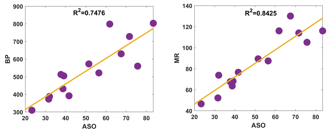
Figure 5: Linear regression plots of A​S​OASO with M​RMR, B​PBP for drug-related compounds.

For M​RMR and B​PBP, equation (35) provides the following models.

B​P=7.2566​(±2.4344)​(A​S​O)+168.5229​(±131.3719),\displaystyle BP=7.2566(\pm 2.4344)(ASO)+168.5229(\pm 131.3719), (38)
R2=0.7476,R​M​S​E=76.1290,F=35.5432,S​F=6.59×10⁻⁵,\displaystyle R^{2}=0.7476,\penalty 10000\ \penalty 10000\ \penalty 10000\ RMSE=76.1290,\penalty 10000\ \penalty 10000\ \penalty 10000\ F=35.5432,\penalty 10000\ \penalty 10000\ \penalty 10000\ SF=6.59\times 10^{-5},
M​R=1.2886​(±0.3217)​(A​S​O)+20.6520​(±17.3624),\displaystyle MR=1.2886(\pm 0.3217)(ASO)+20.6520(\pm 17.3624), (39)
R2=0.8425,R​M​S​E=10.0614,F=64.1693,S​F=3.71×10⁻⁶.\displaystyle R^{2}=0.8425,\penalty 10000\ \penalty 10000\ \penalty 10000\ RMSE=10.0614,\penalty 10000\ \penalty 10000\ \penalty 10000\ F=64.1693,\penalty 10000\ \penalty 10000\ \penalty 10000\ SF=3.71\times 10^{-6}.

The models (38) and (39) indicate that the A​S​OASO index accounts for 75% of the variation in B​PBP and 84% of the variation in M​RMR. These relationships are illustrated in Figure 5. Other evaluated parameters also support the conclusion that the A​S​OASO index effectively predicts both B​PBP and M​RMR. A closer comparison between B​PBP and M​RMR suggests that the index predicts M​RMR more accurately. In Figure 5, the pink circles for M​RMR lie closer to the orange regression line than those for B​PBP, and the associated R​M​S​ERMSE for M​RMR is lower while the FF value is higher. Therefore, the A​S​OASO index demonstrates better predictive performance for M​RMR than for B​PBP.

Comparative Analysis

This subsection compares the A​S​OASO index with several of its variants, including S​OSO (Sombor index), E​S​OESO (elliptic Sombor index), and E​UEU (Euler Sombor index). For this comparison, the indices are correlated with selected physicochemical properties of BHCs and molecular graphs that are relevant to drug design.

The absolute correlation coefficients of A​S​OASO, S​OSO, E​S​OESO, and E​UEU with the physicochemical properties B​PBP and EπE_{\pi} for a dataset of BHCs are displayed in Figures 6 and 7. Similarly, the absolute correlation coefficients between these indices and the physicochemical properties B​PBP and M​RMR for a dataset of molecular graphs associated with drug design are shown in Figures 8 and 9.

For the set of BHCs, considering both B​PBP and EπE_{\pi}, it is observed from Figures 6 and 7 that the absolute correlation coefficients of the studied topological indices follow the order

A​S​O>S​O>E​U>E​S​O.ASO>SO>EU>ESO.

In contrast, for the selected molecular graphs related to drug design, considering both B​PBP and M​RMR, it is observed from Figures 8 and 9 that the corresponding order of correlation strength is

A​S​O>E​U>S​O>E​S​O.ASO>EU>SO>ESO.

These observations indicate that the A​S​OASO index exhibits the strongest correlation, suggesting that it may more effectively reflect the structural characteristics associated with the physicochemical properties of both BHCs and drug-relevant molecular graphs.

Refer to caption
Figure 6: Absolute correlation plot: B​PBP versus selected topological indices.
Refer to caption
Figure 7: Absolute correlation plot: EπE_{\pi} versus selected topological indices.
Refer to caption
Figure 8: Absolute correlation plot: M​RMR versus selected topological indices.
Refer to caption
Figure 9: Absolute correlation plot: B​PBP versus selected topological indices.

4 Concluding Remarks and Future Work

In this paper, we investigated the augmented Sombor index (A​S​OASO) from both theoretical and chemical perspectives. Several sharp bounds for the A​S​OASO index were established over important graph classes, and the corresponding extremal structures were completely characterized. In particular, we identified the minimum value of the A​S​OASO index for unicyclic graphs with a given girth and determined the unique graphs attaining this bound. Moreover, the second maximum A​S​OASO value among trees was obtained, together with a characterization of the extremal tree. We also derived the minimum and maximum values of A​S​OASO for bipartite graphs and chemical graphs and identified all extremal graphs achieving these values. In addition, maximal chemical trees with respect to the A​S​OASO index were characterized. From the chemical viewpoint, the applicability of the A​S​OASO index was examined via quantitative structure–property relationship (QSPR) analysis. The results indicate that the A​S​OASO index shows strong predictive ability for relevant physicochemical properties, confirming its effectiveness as a molecular descriptor.

Motivated by the extremal results obtained in this work, we further propose a conjecture concerning the maximum value of the A​S​OASO index over multipartite graphs. Recall that the Turán graph Tn​(k)T_{n}(k) is the complete kk-partite graph of order nn whose partition sets differ in size by at most one. We conjecture that Tn​(k)T_{n}(k) attains the maximum A​S​OASO value among all kk-partite graphs of order nn. If this conjecture holds, then the conclusion of Theorem 2.8 follows as a special case.

Conjecture 4.1.

For any kk-partite graph Ω\Omega of order nn,

A​S​O​(Ω)\displaystyle ASO(\Omega) ≤r​(k−r)​⌈nk⌉​⌊nk⌋​(n−⌈nk⌉)2+(n−⌊nk⌋)2n−2+(r2)​⌈nk⌉2​n−⌈nk⌉n−⌈nk⌉−1\displaystyle\leq r(k-r)\Big\lceil\frac{n}{k}\Big\rceil\Big\lfloor\frac{n}{k}\Big\rfloor\sqrt{\frac{\left(n-\lceil\frac{n}{k}\rceil\right)^{2}+\left(n-\lfloor\frac{n}{k}\rfloor\right)^{2}}{n-2}}+\binom{r}{2}\Big\lceil\frac{n}{k}\Big\rceil^{2}\frac{n-\lceil\frac{n}{k}\rceil}{\sqrt{n-\lceil\frac{n}{k}\rceil-1}}
+(k−r2)​⌊nk⌋2​n−⌊nk⌋n−⌊nk⌋−1\displaystyle\penalty 10000\ \penalty 10000\ \penalty 10000\ \penalty 10000\ +\binom{k-r}{2}\Big\lfloor\frac{n}{k}\Big\rfloor^{2}\frac{n-\lfloor\frac{n}{k}\rfloor}{n-\lfloor\frac{n}{k}\rfloor-1}

with equality if and only if G≅Tn​(k)G\cong T_{n}(k).

Future research may extend the study of the augmented Sombor index to other graph classes and explore further extremal problems and chemical applications.

References

  • [1] S. Ahmad, K.C. Das, General Sombor index: A study of branching in trees and solution for maximal trees with prescribed maximum degree, J. Combin. Opti. 50 (2025) #21.
  • [2] S. Ahmad, K.C. Das, R. Farooq, On Elliptic Sombor Index with Applications, B. Malays. Math. Sci. So. 48 (2025) #108.
  • [3] S. Ahmad, R. Farooq, K.C. Das, The general Sombor index of extremal trees with a given maximum degree, MATCH Commun. Math. Comput. Chem. 94 (2025) 825–853.
  • [4] A. Ali, A.A. Bhatti, Z. Raza, Further inequalities between vertex degree-based topological indices, Int. J. Appl. Comput. Math. 3 (2017) 1921–1930.
  • [5] A. Ali, K.C. Das, A.M. Alanazi, I. Tomescu, On Diameter-Constrained Unicyclic Graphs and BID Indices, Mediterr. J. Math. 23 (2026) 41.
  • [6] A. Ali, Z. Raza, A. A. Bhatti, Extremal pentagonal chains with respect to bond incident degree indices, Canad. J. Chem. 94 (2016) 870–876.
  • [7] B. Borovičanin, K.C. Das, B. Furtula, I. Gutman, Bounds for Zagreb indices, MATCH Commun. Math. Comput. Chem. 78 (2017) 17–100.
  • [8] K.C. Das, On the vertex degree function of graphs, Comput. Appl. Math. 44 (2025) #183.
  • [9] K.C. Das, Open problems on Sombor index of unicyclic and bicyclic graphs, Appl. Math. Comput. 473 (2024) #128644.
  • [10] K.C. Das, M. Alharbi, J. Bera, Exponential harmonic index and its applications in structure property modeling, Int. J. Quantum Chem. 125 (2025) #e70099.
  • [11] K.C. Das, A. Ali, On the augmented Sombor index of graphs, MATCH Commun. Math. Comput. Chem. 96 (2026) 587–610.
  • [12] K.C. Das, J. Bera, Resolving open problems on the Euler Sombor index, MATCH Commun. Math. Comput. Chem. 95 (2026) 901–918.
  • [13] K.C. Das, I. Gutman, On Sombor index of trees, Appl. Math. Comput. 412 (2022) #126575.
  • [14] K.C. Das, I. Gutman, A. Ali, Augmented Sombor index, MATCH Commun. Math. Comput. Chem. 95 (2026) 523-547.
  • [15] W. Gao, Extremal trees and molecular trees with respect to the Sombor-index-like graph invariants SO5 and SO6, Czechoslovak Math. J. 74 (149) (2024) 927–941.
  • [16] I. Gutman, Degree based topological indices, Croat. Chem. Acta 86 (2013) 351–361.
  • [17] I. Gutman, Geometric approach to degree based topological indices: Sombor indices, MATCH Commun. Math. Comput. Chem. 86 (2021) 11–16.
  • [18] I. Gutman, B. Furtula, M.S. Oz, Geometric approach to vertex degree-based topological indices– Elliptic Sombor index, theory and application, Int. J. Quantum Chem. 124 (2024) #e27346.
  • [19] B. Horoldagva, C. Xu, On Sombor index of graphs, MATCH Commun. Math. Comput. Chem. 86 (2021) 703-713.
  • [20] S. Javed, A. Sattar, M. Javaid, Extremal unicyclic graphs with fixed leaves via Sombor index, J. Discr. Math. Sci. Cryptogr. 28 (2025) 783–795.
  • [21] Y. Li, H. Liu, R. Zhang, Quasi-tree graphs with the minimal Sombor indices, Czechoslovak Math. J. 72 (147) (2022) 1227–1238.
  • [22] Z. Li, L. Shi, L. Zhang, H. Ren, F. Li, On Sombor index of uniform hypergraphs, MATCH Commun. Comput. Chem. 94 (2025) 229–246.
  • [23] H. Liu, Comparison between Merrifield-Simmons index and some vertex-degree-based topological indices, Comput. Appl. Math. 42 (2023) 89.
  • [24] H. Liu, I. Gutman, L. You, Y. Huang, Sombor index: review of extremal results and bounds, J. Math. Chem. 60 (2022) 771–798.
  • [25] H. Liu, Y. Huang, Sharp bounds on the symmetric division deg index of graphs and line graphs, Comput. Appl. Math. 42 (2023) 285.
  • [26] Y. Lu, Q. Zhou, On hyper-Zagreb index conditions for Hamiltonicity of graphs, Czechoslovak Math. J. 72 (147) (2022) 653–662.
  • [27] B. Lučić, N. Trinajstić, B. Zhou, Comparison between the sum-connectivity index and product-connectivity index for benzenoid hydrocarbons, Chem. Phys. Lett. 475 (2009) 146–148.
  • [28] S. Mondal, K.C. Das, Zagreb connection indices in structure property modelling, J. Appl. Math. Comput. 69 (2023) 3005–3020.
  • [29] S. Mondal, D. Huh, K.C. Das, Role of GA, AG and R in structure-property modelling, Polycyclic Aromat. Compd. (2024) 45 #e2405526.
  • [30] F. Movahedi, Results on the elliptic Sombor index, RAIRO Oper. Res. 59 (2025) 2201–2212.
  • [31] V. Maitreyi, S. Elumalai, S. Balachandran, On the extremal general Sombor index of trees with given pendent vertices, MATCH Commun. Comput. Chem. 92 (2024) 225–248.
  • [32] M. Masre, T. Vetrík, General degree-eccentricity index of trees, Bull. Malays. Math. Sci. Soc. 44 (2021) 2753–2772.
  • [33] M. Miftahurrahman, F. Maulana, Sombor index of non-coprime graphs on generalized quaternion groups, J. Indones. Algebra Soc. 1 (2025) 1–7.
  • [34] M. Mohammadi, H. Barzegar, Bounds for Sombor index using topological and statistical indices, J. Discr. Math. Appl. 10 (2025) 61–85.
  • [35] P. Nithyaa, S. Elumalai, S. Balachandran, M. Masrec, Ordering unicyclic graphs with a fixed girth by Sombor indices, MATCH Commun. Math. Comput. Chem. 92 (2024) 205–224.
  • [36] M.R. Oboudi, Sombor index of a graph and of its subgraphs, MATCH Commun. Comput. Chem. 92 (2024) 697–702.
  • [37] M. Randić, Quantitative structure-property relationship. Boiling points of planar benzenoids, New J. Chem. 20 (1996) 1001–1009.
  • [38] B.A. Ravindrana, Sombor index on trees– A review, MATCH Commun. Comput. Chem. 94 (2025) 291–305.
  • [39] Z. Raza, S. Akhter, S. Mondal, M. Ghorbani, Maximal tree and unicyclic graph for Euler Sombor index with given diameter, AKCE Int. J. Graphs Comb. 22 (2025) 289–304.
  • [40] W.A. Stein, Sage Mathematics Software (Version 6.8), The Sage Development Team, website: http://www.sagemath.org, 2015.
  • [41] S. Sekar, B. Selvaraj, S. Elumalai, H. Liu, Maximum Euler Sombor Index of Unicyclic Graphs with Given Diameter, MATCH Commun. Comput. Chem. 95 (2025) 759-776.
  • [42] M.C. Shanmukha, N.S. Basavarajappa, K.C. Shilpa, A. Usha, Degree-based topological indices on anticancer drugs with QSPR analysis, Heliyon 6 (2020) #e04235.
  • [43] V.S. Shigehalli, S.A. Chougale, Sombor index and its applications, Open J. Discr. Appl. Math. 8 (2025) 50–63.
  • [44] C. Xu, B. Horoldagva, L. Buyantogokh, The exponential second Zagreb index of (n,m)(n,m)-graphs, Mediterr. J. Math. 20 (2023) #181.
  • [45] C. Xu, G. Li, Maximum values of Sombor index of bicyclic graphs with a given matching number, RAIRO-Theor. Inf. Appl. 57 (2023) #11.
  • [46] F. Yang, M. Lu, J. Guo, On the minimum Kirchhoff index of unicyclic graphs with given girth and diameter, Bull. Malays. Math. Sci. Soc. 45 (2022) 1287–1299.
  • [47] X. Zhang, S. Noureen, S. Kamran, S. M. Ibrahim, A. Aslam, Sombor indices in main group metal chemistry: Computational evaluation of bismuth(III) iodide, oxide/silicate frameworks, and dendrimers for QSAR applications, Main Group Metal Chem. 48 (2025) #20250011.
  • [48] Q. Zhang, F. Tchier, Z. Hussain, A. Aslam, X. Zuo, On the bounds for the Euler Sombor index of molecular trees and its applications, J. Appl. Math. Comput. 71 (2025) 645-633.