Non-invertible symmetries
in the axiverse, and the imaginary wormholes
Daniele Licciardello & Luca Martucci
Dipartimento di Fisica e Astronomia “Galileo Galilei”, Università di Padova,
& INFN Sezione di Padova, Via F. Marzolo 8, 35131 Padova, Italy
Abstract
We study the symmetry structure of four-dimensional axiverse effective field theories with multiple axions coupled to abelian gauge sectors, including their extensions to broad classes of models. We identify the invertible and non-invertible generalized symmetries, and discuss the associated symmetry-breaking mechanisms together with the resulting hierarchies of energy scales. In particular, we discuss the quantum-gravitational breaking of non-invertible axion shift symmetries predicted by the existence of wormholes and the recently proposed Imaginary Distance Bound. In axiverses, these wormhole-based arguments imply that towers of BPS EFT instantons play a distinguished role and generate infinitely many superpotential terms.
Contents
1 Introduction
From a bottom-up viewpoint, light axion-like fields are motivated by several important questions in particle phenomenology. In particular, they furnish an appealing mechanism for solving the strong CP problem [118, 136, 138], have long been considered viable dark matter candidates [83], and may also participate in inflationary dynamics [55]. It has also been understood since the early 1980s that such light degrees of freedom arise naturally in string theory constructions; see [131] for a review. Indeed, the number of axions present in the low-energy theory can easily be of order hundreds, or even thousands. Models with axions therefore exhibit a very rich phenomenology and are commonly referred to as the axiverse [12]; see [106] for a recent review.
Before incorporating effects associated with a UV quantum gravity completion, it is useful to analyze axiverse models as low-energy effective field theories in their own right. A natural first step is to identify their structural properties and, in this respect, global symmetries provide particularly valuable information, as they strongly constrain the dynamics. Of course, global symmetries are expected to be broken, and hence can at most be regarded as approximate, once the theory is embedded into quantum gravity [110, 67, 14, 66]; see also [65, 123]. Within the Swampland program [132, 114], reviewed for instance in [22, 116, 133, 64, 65, 5, 134, 123], this expectation is usually formulated as the “No Global Symmetry Conjecture”. Nevertheless, the emergence of global symmetries in suitable limits can provide a useful organizing principle for understanding the dynamics in those regimes, as well as the possible symmetry-breaking mechanisms.
A particularly powerful framework for this analysis is the generalized notion of symmetry introduced in [60], in which global symmetries are encoded by extended topological operators. In this formulation, codimension- topological defects generate -form symmetries, with ordinary global symmetries corresponding to . This perspective has led to a much broader understanding of the symmetry structures in quantum field theory. Among the most important examples are non-invertible, or categorical, symmetries, generated by topological defects that do not possess inverses under fusion. These symmetries have been intensely studied in recent years; for reviews and further references, see [34, 107, 54, 63, 127, 24, 21, 129, 99, 27, 40]. Their role in quantum gravity settings has also been investigated in several works, including [125, 71, 109, 38, 70, 126, 15, 57, 9].
The goal of this paper is two-fold. First, we determine the maximal global symmetry structure of general four-dimensional axiverse models with no supersymmetry or minimal supersymmetry, initially leaving aside quantum gravity constraints. We focus in particular on continuous invertible symmetries and on quasi-continuous non-invertible ones, whose parameters can take arbitrarily dense rational values, since these impose the strongest constraints. In this context, quasi-continuous axion shift symmetries are especially important: even when ordinary invertible axion shift symmetries are absent, they can forbid the generation of a non-trivial axion potential and account for its natural smallness, as in [39, 30].
Our second goal is to begin a systematic analysis of quantum-gravitational symmetry breaking mechanisms. In particular, we study the consequences for axiverse models of the recent perspective on axion wormholes proposed in [45, 100] and of the corresponding Imaginary Distance Bound.
We pursue the first objective by considering general axiverse theories containing an arbitrary number of axions together with an arbitrary number of abelian U(1) gauge fields. We also include Gauss-Bonnet and Pontryagin curvature-squared couplings, and comment on the possible effects of non-abelian gauge sectors and additional matter sectors. Our results build on and extend earlier work on the axion-Maxwell theory [29, 39, 30, 142], making use of the framework developed for more general Gaillard–Zumino models in [9]; see also [81] for related work. We will provide a general construction of the relevant non-invertible topological operators. As in [30], see also [23, 128], this construction makes manifest their interplay with invertible higher-form symmetries and leads to hierarchies among the corresponding symmetry breaking scales.
As mentioned above, our discussion of symmetry-breaking effects induced by quantum gravity will significantly rely on the novel viewpoint on axion wormholes proposed in [45, 100]. In the axiverse theories considered here, both invertible and non-invertible axion shift symmetries are tied to the presence of wormholes connecting two asymptotically flat regions, of the kind first constructed in [62]. Such configurations may be reinterpreted as wormhole saddles with imaginary axion profiles, interpolating between imaginary Dirichlet boundary conditions imposed at the two asymptotic ends. The same interpretation extends to more general wormhole solutions [11]; in what follows we will refer to this type of configurations as imaginary wormholes. The papers [45, 100], providing complementary arguments, propose that the appearance of these saddles signals a breakdown of the original effective description and therefore points to the need for its modification, which in particular breaks the axion shift symmetries. More precisely, the total distance between the asymptotic wormhole boundary conditions sets the Imaginary Distance Bound (IDB), below which the analytic continuation of the symmetry-breaking corrections must become relevant.
In this paper we assume the validity of the viewpoint proposed in [45, 100] and explore its consequences for our axiverse models. As we will see, the strongest results can be obtained within the axiverse framework introduced in [93, 94, 95], which captures broad classes of string compactifications. In particular, a distinguished role in realizing the IDB will be played by a special class of BPS fundamental instantons, the EFT instantons as defined in [94, 104].
The paper is organized as follows. In Section 2 we introduce the general four-dimensional axiverse effective field theories studied in this work, including their extension. In Section 3 we determine their invertible and non-invertible global symmetries, construct the corresponding topological operators, and describe the associated charged operators. In Sections 4 and 5 we discuss the possible symmetry-breaking mechanisms and the corresponding hierarchies. In Section 6 we discuss the implications of the viewpoint proposed in [45, 100] and the associated Imaginary Distance Bound. Finally, Section 7 contains our conclusions and possible future directions.
2 Axiverse models
In this section we will describe the axiverse effective field theories (EFTs) on which we will base our discussion. We will first consider non-supersymmetric models, and later describe the relevant features of their minimal supersymmetric extensions. In this section, we will not include any effective potential, or superpotential, for the axion sector. As we will see in Section 3, this requirement can be rephrased in terms of the existence of generically non-invertible axion shift symmetries.111In this section we will just consider the most relevant fields and couplings, but the results of Section 3 hold also more generically, as long as the additional sector is not charged under the U(1) gauge fields, and any additional EFT coupling involves the axions only through their derivatives.
2.1 Basic models
Our models include axions , , with integral peridicity
| (2.1) |
The “angular” variables often used to denote axions are related to our fields via . Furthermore, we also include U(1) gauge fields , , and the corresponding field strengths . We will assume the standard normalization
| (2.2) |
Our ‘minimal’ axiverse EFT takes the form
| (2.3) |
Here is a reference mass scale, so that the axion kinetic matrix is dimensionless.222In terms of the -periodic axions , the first term in (2.3) can be rewritten as , with . The square roots of the eigenvalues of the kinetic metric determine the standard axion decay constants of the canonically normalized axion fields in the basis in which the kinetic metric is diagonal. In a gravitational context, we will identify it with the Planck mass: . Similarly, the dimensionless kinetic matrix determines the U(1) gauge couplings. In the non-supersymmetric models discussed in this subsection, and are constant, while in the supersymmetric models of Section 2.2 they will be promoted to be field dependent. We assume that the spacetime admits a spin structure, so that the last term in (2.3) is compatible with (2.1) only if
| (2.4) |
Non-abelian gauge sectors, such as QCD or GUT sectors, could be added to (2.3). If they couple to the axions through theta-like terms, they generically have important effects. These effects can be straightforwardly taken into account at a later stage. Hence, to avoid overloading the presentation, we will mostly assume the absence of non-abelian sectors, only occasionally commenting on their effects, and relegating more details to the Appendix D.
We also implicitly allow for the inclusion of other sectors, as long as they only introduce derivative axion interactions. In particular, one can add matter charged under the abelian (and non-abelian) gauge groups. This will only be relevant for the discussions of Section 3.3 and part of Section 4, while it will not affect the rest of the paper.
While we will mostly work at the two-derivative EFT level, we will also consider curvature-squared terms, and in particular terms involving the Gauss-Bonnet and the Pontryagin density. The Gauss-Bonnet term takes the form
| (2.5) |
where is the Gauss-Bonnet density
| (2.6) |
As for the kinetic matrices, here the coupling appearing in (2.5) is a constant, while in the models of Section 2.2 it will be allowed to be field dependent. Notice that, in presence of the Einstein Hilbert term, other curvature-squared corrections of the form and can be reabsorbed by a metric redefinition (up to the possible generation of other types of four-derivative corrections). The Gauss-Bonnet density (2.6) is singled out by the special property that, for constant , its integral over a closed Euclidean space computes its Euler characteristic – see e.g. [104] for more comments about this point.333On spacetimes with boundaries one should also include appropriate boundary counterterms [112], analogous to the Gibbons-Hawking counterterm [61]. However, this technicality will not play any relevant role in the following and so we will keep it implicit.
We also allow for a possible axion-Pontryagin coupling
| (2.7) |
Since integral of the first Pontryagin class over a spin four-manifold is a multiple of 48, consistency with (2.1) requires that
| (2.8) |
We will also exploit the description in which the axions are dualized to two-form gauge potentials . In Lorentzian signature, and at the classical level, the relation between these equivalent descriptions is provided by
| (2.9) |
where are the three-form field strengths of the two-form potentials . As recently emphasized in [141], at the quantum level the duality works in a more subtle way.
In the dual description, the last two terms in (2.3) are replaced by
| (2.10) |
where is the inverse of . In particular, the last term in (2.3) and the Pontryagin term (2.7) are encoded in the modified Bianchi identities
| (2.11) |
where444The inclusion of non-abelian gauge sectors generically modifies this relation. For instance, the addition of the term (D.1) in the axion formulation corresponds to adding the term to the r.h.s of (2.12).
| (2.12) |
This implies that the two-form gauge potentials are locally defined by
| (2.13) |
where are the Chern-Simons three-forms such that
| (2.14) |
2.2 Supersymmetric extension
We will also consider minimally supersymmetric extensions of the axiverse models introduced in Section 2.1, which we now describe. These extensions will not play any role until Section 4. Thus, some readers may prefer to first read Section 3 and return to this subsection later.
In supersymmetric models the axions combine with corresponding saxions into complex fields
| (2.15) |
which are the lowest components of chiral multiplets. The spectrum also contains the supersymmetric fermionic partners, which, however, will be irrelevant for most of our purposes and will be explicitly taken into account only in Section 6.4.
The kinetic terms of the (s)axionic sector are determined by a Kähler potential , which will be assumed to be invariant under axion shift symmetries, namely to depend on and only through their saxionic combination . In this case the axion kinetic matrix appearing in (2.3) becomes saxion dependent, but does not depend on the axions, and is determined by the Kähler potential via the relation
| (2.16) |
The same matrix also determines the saxion kinetic terms555In the presence of other chiral fields, additional mixing terms could appear. Since these would not affect our main conclusions, they will be ignored in what follows.
| (2.17) |
In a supergravity context, we will set .
The gauge field kinetic terms in (2.3) are also saxion-dependent and are linked by supersymmetry to the non-derivative axion couplings in (2.3)
| (2.18) |
where the ellipses denote possible additional contributions to the gauge couplings, which are either constant or depend on some hidden chiral fields. By supersymmetry, these contributions would require the inclusion of corresponding terms. However, they will not play any role in our discussion.
Similarly, supersymmetry relates the Gauss-Bonnet term (2.5) and the Pontryagin term (2.7) – see e.g. [105] for more details in our same context. In particular, the coupling appearing in (2.5) necessarily takes the form
| (2.19) |
where as in (2.18) the ellipses are terms that are either constant or at most dependent on some hidden chiral fields. Again, by supersymmetry these possible contributions correspond to a modification of (2.7) that will be irrelevant for our purposes.
The self-consistency of the theory requires that the kinetic matrices are positive definite on the saxionic domain, that is the set of possible values of . If the ellipses in (2.18) are assumed to be , the perturbative regime requires that the saxions are ‘large’ enough, in some appropriate sense.
Most of the results that we will discuss in Sections 3–5 hold for any Kähler potential invariant under axion shift symmetries, and gauge couplings of the form (2.18). However, we will later focus on quantum gravity models, which motivates us to restrict ourselves to the more specific, though still quite broad, framework introduced in [93, 94, 95] and further developed in [105, 104]. This framework covers large classes of string theory models and allows for the identification of a well defined large saxion regime. In this regime the ellipses in (2.18) and (2.19) are subleading and the Kähler potential gets a leading contribution of the form
| (2.20) |
with a homogeneous function of positive integral degree :
| (2.21) |
The integrality of is just an assumption motivated by experience from string theory, with no clear bottom-up motivation. We emphasize that the Kähler potential (2.20) can generically receive subleading corrections. Formally, these are corrections that vanish in the scaling limit with . As we will see, for our purposes we can safely ignore these types of corrections.
Note that this structure naturally leads one to consider conical saxionic domains, namely domains that are preserved under arbitrary rescalings , with . We will denote this conical domain as and refer to it as the saxionic cone. As in [93, 94, 95], motivated by string theory examples, one can consider more structured saxionic cones, imposing that is convex and rational polyhedral. A prototypical example of is the Kähler cone of a Calabi–Yau compactification in string theory. We refer to Section 2.3 for more explicit examples and to Figure 1 for a visual illustration. In order to define more explicitly a saxionic cone satisfying these conditions, it is convenient to adopt a basis independent notation, in which we introduce an -dimensional lattice , which can be considered as the integral subset of a corresponding real vector space . The saxions can be identified with the components of the vector , while the axions are the components of the representative of an element of . The saxionic cone is convex if implies that , and is rational polyhedral if it is generated by a set of integral vectors . Alternatively, it satisfies these properties if
| (2.22) |
where is a subset of integral dual vectors with , and is the canonical pairing between and , namely
| (2.23) |
Notice that the positivity of the gauge couplings (2.18) for large saxions requires that the matrix is positive definite for any .
It is clear that encodes the entire information of , but also that different choices of can give the same . For instance, if both have positive pairing with , then also has positive pairing and could be added to without changing . We will then define as the maximal subset of elements such that for any . Namely, we can alternatively identify with the discretized cone dual to :
| (2.24) |
The choice of the symbol was introduced in [93, 94] and was motivated by the fact that can be identified with the set of possible mutually BPS instanton charges. These are the charges that can be carried by possible BPS instantons, which may modify the EFT by terms involving the chiral operators
| (2.25) |
The condition (2.22) is equivalent to requiring that for any and . In particular, it implies that is exponentially suppressed in the scaling limit with .
Terms of this form can, for instance, be generated by an additional confining gauge sector, or by fundamental instantons that do not admit a field-theoretic interpretation, such as world-sheet instantons in the above-mentioned Calabi–Yau compactifications, or brane instantons in more general string compactifications. At the rigid EFT level, there is nothing that forbids setting all such instanton contributions to zero. In Section 6, we will discuss how, from a purely bottom-up perspective, this is no longer possible in a quantum gravity setting.
It will also be useful to summarize some aspects of the formulation in which the chiral multiplets are dualized by linear multiplets – see [92] for more details about the general formulation, and [93, 94, 105, 104] for related comments about the class of quantum gravity models that we will consider. The linear multiplets contain the two-form potentials dual to the axions , introduced at the end of Section 2.1.666At the quantum level, the duality between these two descriptions requires a counterterm involving the Gauss-Bonnet density (2.6) [46, 141]. Such a term can be reabsorbed in the subleading ellipses in (2.19). Furthermore, they also include real scalars , which provide an alternative parametrization of the saxionic directions. They are related to the saxions by
| (2.26) |
We will refer to them as dual saxions. Note that identify the components of a vector . We will denote by the image of the saxionic cone under the map (2.26):
| (2.27) |
By using (2.20) and the homogeneity (2.21), it is easy to see that is also a cone, in the sense that if , then for any . For this reason we will refer to as the dual saxionic cone – see Figure 1 below for an example.
Note also that, using (2.16) and (2.21), one can easily derive the relations
| (2.28) |
where is the inverse of . The inverse metric appears in the kinetic terms of and – see [92, 94] for more details. Note that, using again the homogeneity of , (2.28) implies that
| (2.29) |
Here and in the following the norms of elements of and are computed by using the metrics and , respectively. That is, in the present case, and .
Finally, we recall that the dual description is more directly formulated in terms of the dual kinetic potential
| (2.30) |
For example, it provides the inverse of (2.26),
| (2.31) |
and the inverse saxionic metric,
| (2.32) |
The general relation (2.30), that holds for general Kähler potential that are invariant under axion shift symmetries, becomes simpler by assuming the homogeneity condition (2.21). Indeed, (2.29) implies that, omitting an irrelevant additional constant, the dual saxion kinetic potential (2.30) takes the form
| (2.33) |
where . Notice that is homogeneous too:
| (2.34) |
We emphazise that, given such a theory with homogeneity , one may consider (s)axionic subsectors with homogeneity . One can identify these subsectors by considering limits in which some subset of saxions become much larger than the other, or some subset of dual saxions become much smaller than the others. If this limit gives a consistent decoupling of the former set from the latter, we can use it to describe a theory with reduced homogeneity degree. In the following Subsection we will provide some examples of how this can work.
2.3 Simple examples
It is useful to discuss possible concrete realizations of the general class of models introduced in Section 2.2, as well as their possible string theory interpretation. We will be brief here; more details and other examples within the same framework can be found in [94, 105, 104].
The simplest example contains just one (s)axion , with saxionic cone . In this case we necessarily have , that is . The dual saxion is then given by , and the dual kinetic potential is , that is . For instance, the Kähler potential of heterotic compactifications on Calabi-Yau three-folds at weak string coupling contains such a contribution with , where parametrizes the four-dimensional dilaton.
In the large volume regime of these heterotic compactifications, one can add saxions , which are the kähler moduli that parameterize the (string frame) Kähler cone of the Calabi-Yau. These combine with the saxion introduced above to parametrize an dimensional saxionic cone . This can be represented as a fibration where the fiber is a one-dimensional cone parametrized by , with , and the base is the Kähler cone parametrized by the saxions [105, 104]. Here are constant integers and we can assume that . The Kähler potential is
| (2.35) |
where are the Calabi-Yau triple intersection numbers. Hence, we have enlarged the homogeneity from to . By considering the limit , one can consistently focus on the one-dimensional subsector parametrized by , thereby recovering the theory discussed above. On the other hand, the condition generically obstructs taking a large (string-frame) volume limit in which all the saxions become much larger than . Therefore, one cannot simply focus on the while keeping fixed.777See [89, 90] for a detailed analysis of similar obstructions in type IIB/F-theory models. Nevertheless, other asymptotic limits can be considered, leading to different consistent saxionic subsectors. For instance, in heterotic models admitting an F-theory dual, one may focus on a saxionic subsector with effective homogeneity , corresponding to the F-theory models discussed in the next paragraph – see [104, App. B] for further details about this relation.
In F-theory compactification at large volume, the Kähler moduli are parametrized by a set of dual saxions , where is the base three-fold of the associated elliptically fibered Calabi-Yau four-fold. In the kinetic potential (2.33) we must take
| (2.36) |
where are the triple intersection numbers of . Clearly, in this case we have . The saxionic cone and dual saxionic is model dependent.


For instance, consider the case in which is a fibration over , with twist parameter . In this case we have two dual saxions , parametrizing the dual saxionic cone – see Fig. 1(b) – and
| (2.37) |
The corresponding saxions can be obtained from (2.31) and parametrize the saxionic cone – see Figure 1(a). Notice that, even if (2.37) has homogeneity , we could consider the limit in which and focus just on the subsector parametrized by , with , so that we effectively have . Indeed, the limit corresponds to an infinite field distance limit in which the F-theory model is dual to a weakly-coupled heterotic compactification of the type discussed above, with . On the other hand, we cannot do the same by taking , which is instead a finite distance limit.
3 Non-invertible symmetries in the axiverse
In this section, we discuss the invertible and non-invertible global symmetries, together with the corresponding topological defects and charged operators, of the axiverse models described in Section 2. We follow a ‘descending’ order, starting with the two-form symmetries and then turning to the one- and zero-form symmetries. This organization allows us to begin with the invertible symmetries and helps clarify the relations among the various defects. Supersymmetry plays no role in the present discussion. The results presented here can be regarded as an axiverse generalization of previous analyses of the axion-Maxwell model [29, 39, 30, 142, 43], see also [78, 79, 80], and [81] for previous work considering axiverse settings. For the invertible symmetries discussed in Sections 3.1 and 3.2, the generalization is essentially straightforward. By contrast, the axiverse generalization of the non-invertible symmetries discussed in Sections 3.3 and 3.4 is less obvious, and builds on and extends the techniques introduced in [104] to describe the non-invertible symmetries of more general Gaillard-Zumino models [58].
3.1 Winding two-form symmetries and vortex operators
We start our discussion of the global axiverse symmetries by considering the winding two-form symmetries. They are associated with the one-form conserved currents
| (3.1) |
In our notation the Noether current of a continuous -form symmetry is given by a closed -form – such that – rather than by its Hodge dual -form. The winding two-form symmetries are realized by codimension-three topological operators
| (3.2) |
which are supported on one-dimensional curves . The periodic parameters label the corresponding U(1) element.
The winding topological operator (3.2) acts on codimension-two extended operators, supported on two-dimensional surfaces . These operators can be defined by excising a small tubular neighborhood of and imposing that the axions undergo an integral shift
| (3.3) |
around them. We will denote these operators as , where the charge vector takes values in the lattice , and we will refer to them as vortex operator. The axion winding (3.3) condition implies that the insertion of modifies the conservation equation into
| (3.4) |
which encodes the contact term contribution appearing in Ward identities for the winding two-form symmetry. Hence, if is a circle that links , we get
| (3.5) |
where we have used the index-free notation for the pairing between and , with denoting the dual of , and and are the corresponding integral lattices.
Importantly, as emphasized e.g. in [30], the surface operator must support a non-trivial world-sheet sector. This is because of the anomaly inflow mechanism [26, 113] – see also [56, 53, 74, 105]. The sum of the last term in (2.3) and (2.7) can be rewritten as
| (3.6) |
where are the Chern-Simons three-form defined in (2.14). These are not invariant under infinitesimal gauge and local Lorentz transformation:
| (3.7) |
Hence, (3.4) produces the following anomalous contribution localized on :
| (3.8) |
This can alternatively be understood in the dual formulation introduced at the end of Section 2.1, in which the axion vortex supports the coupling . Then (3.8) follows from (2.13) and the gauge invariance of .
The anomaly (3.8) must be canceled by a world-sheet anomaly.888In a QFT setup in which gravity is not dynamical, we could allow for a non-vanishing ’t Hooft gravitational anomaly, captured by the last term in (2.14). However, having in mind the eventual coupling to dynamical gravity, for later convenience we keep this condition as one of the defining properties of . Hence, must support a non-trivial world-sheet sector including chiral fermions or bosons, whose anomaly polynomial under bulk gauge and local Lorentz transformations is precisely given by . See [105, Section 3.2] for more details in a very similar setting – though considering dynamical axion strings rather than codimension-two operators – including also the contribution of non-abelian gauge sectors as in Footnote 4. Note that, for any anomaly polynomial , the choice of the worldsheet degrees of freedom is not unique. However, we will not need to specify them and will denote any such operator.
3.2 Magnetic one-form symmetries and ’t Hooft lines
The magnetic one-form symmetries of our axiverse model are generated by the two-form currents . The corresponding U(1) one-form symmetries are realized by the invertible topological operator
| (3.9) |
and labeled by the periodic parameters . The associated charged operators are provided by ‘t Hooft lines carrying magnetic charges , whose insertion modifies the Bianchi identity into
| (3.10) |
These ’t Hooft lines can be defined by excising a small tubular neighborhood of and imposing that
| (3.11) |
along it. So, if we pick a two-sphere linking we have
| (3.12) |
Here we are again using an index free notation for the canonical pairing between and , where denotes the lattice of magnetic charges, the corresponding real vector space, and and the associated duals.
Analogously to what happens for the vortex operators in Section 3.1, and what discussed in [56, 53, 30] for the axion-Maxwell model, ’t Hooft lines must support a non-trivial world-line sector. This basically comes from the Witten effect [139], namely the fact that monopoles acquire electric charge under a shift of the theta-angle, and can also be understood as an anomaly inflow [35, 36, 56]. In our framework, this inflow produces an anomalous behavior under integral axion shifts , . One way to see it is to compute from (2.3) the dual field strengths
| (3.13) |
An ’t Hooft line should contain the factor , where are the dual magnetic potentials, such that . However, from (3.13) it is clear that the field strengths , and hence the magnetic potentials , are not invariant under integral axion shifts. More precisely,
| (3.14) |
under , and hence acquires an anomalous phase
| (3.15) |
which must be canceled by a non-trivial world-line sector. The choice of this sector is not unique, but a simple realization [84] is obtained by introducing a set of periodic world-line axions , providing a many-body generalization of the particle-on-a-circle quantum mechanics [35, 59]. These world-line axions couple to the bulk fields through the world-line partition function
| (3.16) |
where is the world-line kinetic matrix and
| (3.17) |
Gauge invariance requires that under the gauge transformation . It is clear that, under the bulk axion shift , the second term in (3.16) produces an anomalous phase that precisely cancels (3.15). We emphasise that the choice (3.16) is not the only possible one. Furthermore, it is not even uniquely defined by itself, since is arbitrary.
3.3 Non-invertible electric one-form symmetries
We now turn to the non-invertible symmetries present in our class of models. The results of the previous two subsections remain valid in the presence of fields charged under the U(1) gauge fields. Throughout this subsection, we assume that electrically charged particles are absent, since their presence would partially or completely break the electric one-form symmetries; see Section 4.3.
If the axions were not periodic, we could identify the two-form electric currents with the dual field strengths defined in (3.13). However, as already emphasized in Section 3.2, the are not invariant under the axion periodicity and therefore cannot be used as gauge-invariant two-form currents. As we are going to discuss, one can generalize the construction presented in [30] for axion–Maxwell theory to show that most of the electric one-form symmetries are not lost: rather, a dense subset of them survives, albeit in a non-invertible form.
More precisely, one can construct a topological defect for each , where is the lattice of magnetic monopole charges, and is its -span. In other words, is labeled by , with . We will first define for any , and then argue that it is topological.
In order to define , let us first introduce the matrix of components
| (3.18) |
Since (see (2.4)), it is clear that for any (and for any ). As discussed in Appendix A, one can then always pick a right-coprime factorization
| (3.19) |
in terms of integral matrices
| (3.20) |
An algorithm for explicitly identifying a right-coprime factorization is described in Appendix A.1. In components, (3.19) reads , and we keep implicit the dependence of and on the axion shift vector . As discussed in Appendix A, being right-coprime, and are unique, up to an unimodular transformation
| (3.21) |
Notice that, in particular, if , then we can just pick and .
The defect can then be defined as follows,
| (3.22) |
where
| (3.23) |
and we have introduced compact scalar fields and U(1) one-form vector fields , all living on . Notice that the two-form current is gauge invariant but not conserved:
| (3.24) |
The analogous defect constructed in [30] for the axion-Maxwell model can be regarded as the subcase of (3.22).
It is clear that (3.22) is well defined, since all the coefficients appearing in the path-integrated exponential are properly quantized. As in [30], a simple heuristic way to check that (3.22) is topological and provides a realization of the electric one-form symmetry is to try to integrate out the world-sheet fields and . The corresponding equations of motion and can be ‘naively’ solved by setting and . This solution is naive because it does not respect the appropriate quantization conditions of the world-sheet fields. But by plugging it into (3.22) and taking (3.23) into account, it produces precisely the naive topological operator , supporting the idea that (3.22) does exactly what we need for our purposes. This conclusion can be confirmed by a more conceptual derivation of (3.22) from a half higher gauging [41, 87, 30], carried out in Appendix B, along the lines of what was discussed in [30] for the axion-Maxwell model.
For our purposes, it is sufficient to mention that one must perform a half higher gauging with respect to a discrete subgroup of U(1)U(1). Insight into the structure of this subgroup is provided by studying the fusion , which also highlights the non-invertible nature of this symmetry operator. This fusion is computed in Appendix B.1 and here we just quote the result
| (3.25) |
where for simplicity we have omitted the overall normalization factor. In (3.25) we have introduced the finite subgroups and . So, for instance, an element corresponds to an integral vector , of components , modulo the identification for any .
It is clear that (3.25) can be regarded as a condensation defect [124] involving a finite number of winding two-form and magnetic one-form symmetries. The fact that the fusion (3.25) does not yield the identity reflects the non-invertible nature of (3.22). We also remark that the operator (3.23) does not depend on the specific coprime factorization we choose. Indeed, as already emphasized, different coprime factorizations are related by unimodular transformations (3.21), which can be reabsorbed by the field redefinition . Furthermore, one can explicitly check that (3.22) is invariant under for any , consistently with the fact that it should depend only on mod ; see Appendix C for details. Once again, it is crucial that (3.19) is right-coprime.
We also observe that, if more general are such that , one can again set and , and exactly integrate out as in the previous paragraph. This means that in these cases (3.22) reduces to the invertible operator
| (3.26) |
which is well defined precisely because , and non-trivial if .999In fact, the operator (3.26) is well defined for any set of real parameters such that . This condition selects the group of invertible electric one-form symmetries, which of course strongly depends on . As a trivial example, if , then we have a U group of invertible one-form symmetries, and no non-invertible ones. As another simple case, suppose that and is non-degenerate. Then the invertible electric one-form symmetries form the finite subgroup . More general cases can be analyzed similarly.
Finally, let us discuss the action of the topological defect (3.22) on various operators. First of all, it acts in an invertible way on Wilson lines
| (3.27) |
by measuring their electric charge. Namely, if we pick a two-sphere linking , we have
| (3.28) |
This comes just from the exponential in (3.22) containing , which acts on Wilson lines like . The action on local operators is clearly trivial, since a local operator cannot be linked with a codimension-two defect . By contrast, the action on ’t Hooft lines and vortex operators is more intricate, as already happens in the simpler axion-Maxwell case [30]. We will not discuss the details of this non-trivial action in the present work.
3.4 Non-invertible axion shift symmetries
We finally turn to the non-invertible zero-form symmetries associated with arbitrary rational shifts of the axions. This kind of symmetries were previously studied in the context of the axion-Maxwell model [29, 39, 30, 142], see also [121, 33, 43], and for the more general Gaillard-Zumino models in [9]. As in Section 3.3, we will focus only on the defect operator and its properties, postponing the discussion of physical implications to Sections 4-6.
In the absence of the axion-gauge couplings in (2.3) and axion-Pontryagin couplings (2.7), the action is invariant under a real shift of the axion, for . The associated conserved and gauge invariant currents are
| (3.29) |
where in the second equation we have used the dual formulation, cf. (2.9). However, non-vanishing and in (2.3) and (2.7) break the closure relation (3.29) and hence, at first glance, appear to break the continuous axion shift symmetries. As we will now explain, a dense subgroup of rational axion shift symmetries nevertheless survives, albeit in a non-invertible form.
For the time being, let us focus on the coupling between the axions and the abelian gauge sector by setting . We will return to the axion-Pontryagin coupling later. Then the exterior derivative of (3.29) gives
| (3.30) |
Our aim is to identify a codimension-one topological operator , that implements the axion shift for any , that is for any with . In order to define this operator, let us first introduce the matrix of components
| (3.31) |
Since , the matrix has rational entries, i.e. , for every . We can therefore directly apply the construction of the -defect developed in [9], which in turn generalizes the strategy originally proposed in [29, 39].
First of all, we have to pick a right-coprime factorization (see Appendix A)
| (3.32) |
in terms of integral matrices and , as was done for the electric one-form symmetries discussed in Section 3.3. In this case, is also a square matrix. Obviously, and depend on , but we keep this dependence implicit. As explained in [9], given the right-coprime factorization (3.32), on any oriented three-dimensional submanifold one can define a corresponding minimal [82] topological QFT (TQFT) with one-form symmetry, where (cf. comments below (3.25)), and with corresponding anomaly fixed by . One can couple this theory to , regarded as a background flat connection for the one-form symmetry. We will denote the resulting partition function by .
If were such that , then would simply be the partition function of the three-dimensional Chern–Simons theory
| (3.33) |
where and are world-volume U(1) gauge fields. However, it is not a priori obvious that vectors with this property even exist, and one should generically use more complicated TQFTs, which nevertheless always admit a description in terms of abelian Chern–Simons theories [18]. Alternatively, can be identified more directly with the partition function of the four-dimensional TQFT defined on an auxiliary four-dimensional manifold with boundary . This theory is described by the action
| (3.34) |
where and are dynamical one- and two-form potentials living on Y.
The topological defect realizing a generic rational axion shift symmetry for any can then be obtained by stacking this TQFT on the codimension-one operator :
| (3.35) |
In the following, we will analyze some simple properties of this defect. For the explicit construction, which shows that the defect is topological, we refer to [9].
One first simple but rather important property is the independence of the defect on the specific right-coprime factorization. This can for instance be checked by using (3.34). Any two coprime factorizations are related by a unimodular transformation , as discussed in Appendix A, which can always be reabsorbed by the field redefinition . Furthermore, one can check that (3.35) is invariant under for any , consistently with the fact that (3.35) depends on only through its equivalence class in – see Appendix C.
One can also easily show that if we take such that then the defect assumes a simpler form. In particular, we can choose the factorization and . In this way, we can exactly integrate out the fields in (3.34) and find that (3.35) reduces to
| (3.36) |
Notice that the condition can be satisfied not only for but also, depending on the form of , for more general values . In the former case the operator is trivial, whereas in the latter the corresponding defect is non-trivial, showing that a non-trivial invertible subgroup of U survives.
The topological defect realizes the expected axion shift. Since the axions are periodic, they can enter any local operator only through factors of the form , with and . Picking a three-sphere that surrounds the point , we get
| (3.37) |
From this equation it is clear that (3.35) acts in an invertible way on the charged local operators . On the other hands, when one analyzes the action on extended operators, its non-invertible nature shows up. In particular ’t Hooft lines are mapped to non-genuine line operators, because under the axionic shift the dual field strengths (see (3.13)) are mapped to , which are generally not properly quantized to be identified with U(1) field strengths. See [9] for more details, as well as [29, 39, 30, 142, 43] for the analogous phenomenon in the simpler axion-Maxwell model.
The non-invertible nature of (3.35) also shows up in the fusion . In the particular cases in which admits the simple factorization with , this fusion gives the condensation defect [9]
| (3.38) |
where is the Bockstein image of , and for simplicity we have again omitted the overall normalization. For our purposes, it is important to notice that this condensation defect is non-trivial and involves the magnetic one-form symmetries with parameters in . This shows that the existence of requires the presence of this subgroup of magnetic one-form symmetries. The same conclusion extends to more general , as can also be seen from the half-space gauging construction of [9], which explicitly makes use of the subgroup of magnetic one-form symmetries.
Let us now reconsider the possibility of a non-vanishing axion-Pontryagin coupling (2.7). (According to [105], such a coupling is actually expected to be necessarily present in quantum gravity theories with a non-trivial gauge sector.) This term modifies the non-conservation equation (3.30) by adding the term
| (3.39) |
to its right-hand side. In the presence of a non-flat metric, this appears to render the defect (3.35) non-topological. However, as discussed in [121], this type of violation can be canceled by an appropriate modification of (3.35), which restores its topological nature. Briefly, one can add to the defect the counterterm
| (3.40) |
where is the gravitational Chern-Simons three-form, satisfying . This term, together with the minimal TQFT supported on the defect, introduces a framing anomaly [140] with an overall rational coefficient. This anomaly can then be canceled by stacking the defect with a decoupled TQFT that has an appropriate rational chiral central charge [121].
Finally, as discussed more explicitly in Appendix D, we note that the inclusion of non-abelian sectors generically removes part of the possible non-invertible axion shift symmetries. In what follows, we will continue to assume that these sectors are either absent, or that we have restricted attention to axions that do not couple to them.
4 Symmetry breaking of higher-form symmetries
The models described in Section 2 should generally be regarded as low-energy effective field theories. Hence, the global symmetries discussed in Section 3 may either uplift to global symmetries of the corresponding UV-complete theory or be approximate symmetries emerging in the infrared. Both possibilities can arise when gravity is decoupled. In a quantum gravity context, however, it is widely believed that the former possibility can never occur [110, 14, 66].
The purpose of this section is to discuss the possible mechanisms for breaking higher-form symmetries. Since higher-form symmetries act on extended operators, their breaking cannot occur without introducing new degrees of freedom into the EFT. The breaking of each higher-form symmetry can therefore be associated with the appearance of a corresponding charged sector, characterized by a symmetry-breaking energy scale below which the charged objects cannot be excited.
For each case, we first consider the simpler non-supersymmetric setting of Section 2.1 – see [23, 39, 30, 37, 128] for related discussions of the simpler axion-Maxwell model – and then discuss what additional insights can be gained in the supersymmetric extensions of Section 2.2. Throughout, we will also strive to distinguish clearly between conclusions that rely on conjectural quantum gravity constraints and those that hold more generally.
4.1 Winding symmetry breaking and axion strings
We proceed in the same order as in Section 3, and first consider the invertible winding two-form symmetries. Their breaking requires the existence of dynamical axion strings, namely finite-tension counterparts of the axion vortex operators discussed in Section 3.1. We denote by the set of axion charges populated by physical strings.
From (3.5), a dynamical string with charge vector breaks the winding symmetries with parameters whenever . Hence, for fixed , we can identify the following scale at which the corresponding winding two-form symmetry is certainly broken:
| (4.1) |
where denotes the tension of the lightest string of charge . A rough motivation for (4.1) is the following. At the EFT level, one can consider the nucleation of string loops. For a string not to be resolved below the EFT cutoff , one should have , and the loop radius should satisfy . An estimate of the loop mass is then given by . This suggests that the winding symmetry in the direction can only emerge at energies below . Denoting by the actual symmetry-breaking scale, we get the upper bound
| (4.2) |
In particular, the winding symmetry may be broken at energies much smaller than if the string is not fundamental, namely if it admits a solitonic description within an intermediate four-dimensional EFT; see for instance [23]. On the other hand, in the absence of supersymmetry, little can be said about , and hence about , without knowing something about the UV completion.
In the presence of supersymmetry, more can be said. The tension of BPS strings is fixed by supersymmetry to be [92]
| (4.3) |
where are the dual saxions introduced in (2.26), and in the presence of gravity. Anti-BPS strings instead have tension . For a given string charge vector , we expect BPS strings to be the lightest and most stable ones. Therefore, using (4.3) in (4.1) gives a more explicit expression for the upper bound (4.2).101010In the presence of massless saxions, the interpretation of (4.3) is affected by the saxionic backreaction, which should be appropriately understood as an RG flow along the string [93, 94].
In practice, applying (4.1) requires knowing the spectrum of axion strings, not only their tensions. In quantum gravity models, further information follows from standard quantum gravity expectations. First, the absence of exact global symmetries [110, 14, 66] implies that the set of string charges must generate the entire lattice . Furthermore, the Weak Gravity Conjecture (WGC) [10] for multiple gauge fields [28] – see [65] for a review and more references – implies that the convex hull of the vectors
| (4.4) |
with should contain a ball of radius , as measured by the metric appearing in (2.3). This follows from (2.10), with , since defines the couplings of the dual two-form gauge fields. In particular, the lightest strings are expected to satisfy the WGC bound
| (4.5) |
Hence, for such strings, , which gives the bound
| (4.6) |
The above WGC considerations should hold independently of supersymmetry, but they can be sharpened in the supersymmetric models described in Section 2.2. Using (2.28) and (2.29) in (4.3), the Cauchy–Schwarz inequality gives
| (4.7) |
Thus, in models with Kähler potential (2.20), the BPS string tension (4.3) satisfies a WGC bound (4.5) with . A more detailed discussion on this bound, including the subtleties in the definition of string tension, can be found [93, 94]111111As discussed in [93], (4.7) holds also for more general no-scale models, with , and not just those with Kähler potential (2.20).; see also the recent discussion in [52].
As argued in [93, 94], there is a distinguished subclass of BPS axion strings, the EFT strings, which are genuinely gravitational in nature and have special properties. In particular, they can saturate the WGC bound with . More precisely, the set of EFT string charges can be identified with the discretization of the closure of the saxionic cone introduced in Section 2.2:
| (4.8) |
See Figure 2 for an illustration. Since , the bound (4.7) can be saturated by taking aligned, or arbitrarily close, to the direction identified by .
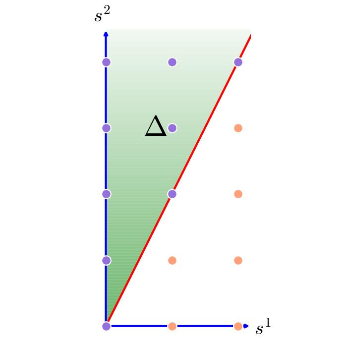
There may exist other BPS strings, filling out a larger set of charges . In concrete string theory compactifications, BPS strings typically arise from higher-dimensional branes or bundles localized on internal supersymmetric cycles. EFT strings are distinguished by their association with “movable” internal configurations, which can recombine and explore the full configuration space [94]. In particular, string theory realizations suggest that only EFT strings generically satisfy completeness, namely, that for each there exists a physical string carrying charge . This would also guarantee that the winding symmetries are fully broken by EFT strings alone, without the need to invoke additional axion strings, whether BPS or not. From the quantum gravity viewpoint, non-EFT strings appear accidental rather than necessary.
Since EFT strings are fundamental, their tension directly sets the corresponding winding symmetry-breaking scale. We may therefore identify the quantum gravity winding symmetry-breaking scale with
| (4.9) |
where we have emphasised the dependence of on the moduli space position. An additional piece of information comes from the relation between EFT strings and the species scale [50, 49, 48, 47], namely the scale at which any EFT description of the gravitational model is expected to break down. As proposed in [104] – see also [17] – this relation is encoded in
| (4.10) |
Applying (4.10) to (4.9), we obtain
| (4.11) |
To summarize, the chain of arguments above suggests that, except for accidental winding-symmetry breaking due to non-EFT strings, genuinely quantum-gravitational breaking occurs at energies above the species scale, as expected. In the presence of non-EFT strings, one may instead have breaking at a lower scale , possibly even below the species scale, but this should not be interpreted as originating from quantum gravity. It would be interesting to develop this idea further, for instance by adapting to our setting the framework recently proposed in [8].
Finally, we recall that, as in [104], completeness and quantum consistency of EFT strings can be used to argue that, in quantum gravity models,
| (4.12) |
where is the rank of the abelian and non-abelian gauge sector detected by the EFT string. In the models of Section 2.2,
| (4.13) |
where the matrix is determined by the couplings (2.18).
4.2 Magnetic one-form symmetry breaking
Similarly to axion strings, dynamical magnetic monopoles, which are the finite mass counterparts of the ’t Hooft lines introduced in Section 3.2, provide the natural mechanism for breaking the invertible magnetic one-form symmetries. We denote by the set of magnetic charges populated by dynamical monopoles. From (3.12), we see that the magnetic one-form symmetry associated with a given choice of is certainly broken at the energy scale
| (4.14) |
where is the mass of the lightest monopole of charge . As for (4.1), is expected to provide only an upper bound on the actual magnetic one-form symmetry-breaking scale :
| (4.15) |
The scale can be significantly smaller than for non-fundamental monopoles that admit a solitonic uplift within an intermediate four-dimensional EFT. For instance, in the SU(2) model giving the ’t Hooft-Polyakov [1, 120] uplift of the Dirac monopole, the magnetic one-form symmetry is broken at the -boson mass , where is the gauge coupling and sets the scalar VEV, while the monopole mass is .
Unlike axion strings, monopoles in models completely break the bulk supersymmetry. Therefore, the computation of their mass depends a priori on details of the UV completion. In quantum gravity models, one may try to invoke the magnetically dual version of the WGC. This would put an upper bound of order on the lightest monopoles, and hence on (4.14). In the weak-coupling regime assumed here, however, this scale is much larger than the Planck mass and therefore does not provide useful information. Some universal features of (4.14) could perhaps be extracted from explicit string-theory constructions. In any case, as in the axion-string case, we expect some subclass of monopoles to stand out as genuinely gravitational, and to set the scale of the quantum-gravitational breaking of the magnetic one-form symmetries. We leave a more detailed investigation of these aspects to future work.
4.3 Electric one-form symmetry breaking and hierarchies
Let us finally turn to the electric one-form symmetry described in Section 3.3. Its breaking is associated with the presence of electrically charged matter, which can be regarded as the finite-mass counterpart of the Wilson lines (3.27). As in the other cases, one should identify the set of electric charges populated by physical particles.
In this case, it is natural to identify the symmetry-breaking scale associated with a given non-invertible topological operator (3.22) with the mass of the lightest particle charged under it. Recalling (3.28), for any we can then define
| (4.16) |
where is the mass of the lightest particle of charge .
As in [30], the non-invertibility of the electric one-form symmetries introduces an interesting correlation between their breaking scales and the symmetry-breaking scales discussed above; see also [23, 128]. Following [30], this correlation can be understood in terms of the condensation defect (3.25), whose definition relies on the magnetic one-form and winding two-form symmetries. More precisely, preserving the electric one-form symmetry in a given direction requires that the winding and magnetic symmetries appearing in its condensation defect remain unbroken. Their parameters take values in the following finite groups:
| (4.17) |
where and were introduced in Section 3.3, and here we emphasize their dependence on . Moreover, the group is the image of into mod , under the linear map defined by the matrix introduced in (3.18). Importantly, the finite groups appearing in (4.17) do not depend on the particular coprime factorization (3.19) one chooses, but only on . Hence, we obtain the hierarchy
| (4.18) |
This hierarchy looks intricate, but it has a clear physical interpretation. Let us first focus on the appearance of . This can be understood by recalling that a monopole of charge vector , like the corresponding ’t Hooft loop, must generically support a world-line sector as in (3.16). This means that it couples to the bulk gauge fields through the combination . This coupling breaks the electric one-form symmetry with parameters mod such that is not an integer, namely such that . Using the right-coprime factorization (3.19), it is easy to see that this is equivalent to requiring . From (3.12), we see that the monopoles satisfying this condition are precisely those that break the magnetic one-form symmetries with mod for some , that is, with . Hence (4.18) simply means that is bounded by the mass of the lightest monopole that breaks the non-invertible electric one-form symmetry identified by .
A similar argument explains the appearance of . Indeed, as already remarked, an axion string of charge vector must contain a chiral world-sheet sector that couples to the bulk gauge fields and produces an anomaly that cancels (3.8). One simple possibility is provided by a set of world-sheet chiral bosons that shift under the bulk gauge symmetries, with corresponding covariant derivative ; see e.g. [113]. This minimal coupling breaks the electric one-form symmetry with parameters mod such that , namely such that . From (3.5), it is clear that the strings that satisfy this condition are precisely those that break the winding symmetries with mod for some , that is, with . Thus (4.18) implies that is also bounded by the energy scale set by the lightest axion string that breaks the non-invertible electric one-form symmetry identified by .
These observations give a clean physical interpretation of the bounds (4.18), make manifest that they do not depend on the choice of coprime factorization (3.19), and provide a non-trivial self-consistency check of the overall framework. Of course, the non-invertible electric one-form symmetry can be broken at energy scales which are smaller than those set by the above monoples and strings, for instance by the appearance of charged matter.
The field-theoretic result (4.18) is universal, but its concrete realization can be strongly model dependent. Introducing quantum gravity input provides further information. First, as in [30, 125, 71], the expected absence of global symmetries [110, 14, 66] requires the set of physical charges to generate the entire lattice , thereby realizing the completeness hypothesis [119, 14]. Furthermore, the WGC [10], in the multifield formulation of [28], imposes upper bounds on ; see [65] for a review and further references. It is also interesting to observe that, in our framework, among the possible axion strings, the non-gravitational ones appear to give the strongest contribution to the upper bound (4.18). Indeed, as recalled in Section 4.1, the species scale sets the lower bound (4.10) on the tension of EFT strings. Hence, their contribution to the right-hand side of (4.18) lies beyond the ultimate quantum-gravity EFT cutoff. It would be interesting to understand whether a similar conclusion holds for the monopole contribution to (4.18). However, since monopoles are not BPS in minimally supersymmetric models, addressing this point probably requires an analysis of concrete string theory constructions.
5 Axion symmetry breaking and naturalness
Compared to the higher-form cases, the breaking of the zero-form symmetries discussed in Section 3.4 is qualitatively very different,121212We thank Luca Vecchi for useful discussions related to these aspects. since it can be encoded in a modification of the local four-dimensional Lagrangian. In particular, in absence of non-minimal supersymmetry, once the axion shift symmetries have been broken, nothing generically prevents the generation of a non-trivial axion potential , e.g. by quantum corrections. This means that the axion shift symmetries of Section 3.4 cannot precisely be regarded as emergent at low energies. Rather, they hold (approximately) at intermediate energy scales between the energy scales set by – say given by the corresponding axion mass – and a symmetry breaking scale that characterizes symmetry breaking effects that are suppressed at energies much lower than , say associated with higher-derivative operators.
So, in order to talk about approximate shift symmetry, we need a hierarchy , which is a priori not guaranteed. In such a case, for energies , the symmetry breaking strength is parametrized by powers of and . The key point is that the axion shift symmetry is restored for and . It is then technically natural [2] to have .
On the other hand, this technical naturalness requires a mechanism that ensures that is small in the first place. In particular, in order to address this point, one should take into account the possible non-trivial constraints which, as in [30], can be associated with the non-invertible nature of the axion shift symmetries. As emphasized in Section 3.4, these zero-form symmetries cannot exist in the absence of magnetic one-form symmetries. This connection is easily seen by considering the condensation defect (3.38). This shows that for a given , defined mod , the topological defect defined in (3.35) requires that the magnetic one-form symmetries with parameters are not broken. We recall that , and we have emphasized the dependence of this discrete group on . By consistency, for any shift symmetry , we get the following upper bounds
| (5.1) | ||||
As for the bound (4.18), (5.1) admits a clear physical interpretation. Recall that, as for the ’t Hooft lines discussed in Section 3.2, monopoles must support a world-line theory like (3.16). Hence, a monopole of charge vector couples to the bulk axions through the combination . This coupling breaks the bulk axion shift symmetries with parameters such that is not an integer, that is, such that . By using the right-coprime factorization (3.32), it is easy to see that this is equivalent to requiring that . The monopoles whose charge vector satisfies this condition are precisely the monopoles that completely break the magnetic one-form symmetries associated with . Hence (5.1) just means that is bounded by the mass of the lightest monopole that breaks the non-invertible shift symmetry identified by .
This physical interpretation of (5.1) also suggests that, in absence of other symmetry breaking sources, we could set . Furthermore, there should exist a mechanism that communicates the magnetic one-form symmetry breaking to , and hence to . Such a mechanism was identified in [53], which discusses how quantum loops of dynamical monopole can induce a non-trivial axion potential. In our framework, this must originate precisely from the interaction between the bulk axions and the monopole world-line sector that was the key to explain (5.1). The relevance of this mechanism in the context of non-invertible axion symmetries has been already emphasized in [39, 37, 30]. Even if we have not worked out a precise form of this potential in our more general axiverse models, it should share the same qualitative features highlighted in [39, 37, 30]. In particular, at weak gauge coupling, the monopole generated axion potential should be exponentially suppressed, hence realizing the technically natural hierarchy .
In any case, as already emphasized, nothing excludes other symmetry breaking contributions which may compete with the monopole ones. So, we may regard the possible IR symmetry breaking scale induced by monopole loops as a setting the lower bound
| (5.2) |
Since at weak coupling should be exponentially suppressed, it is still natural to assume .
Note that, a priori, in axiverse models, these types of monopole effects could not be sufficient to break all axion shift symmetries. For instance, this clearly happens if the number of axions is much larger than the total rank of the gauge sector. Moreover, in minimally supersymmetric models, monopoles cannot be BPS and hence do not seem sufficient to generate a superpotential, and hence a potential. So, the leading contribution to the above symmetry breaking scales could actually have a different origin. In particular, among the various possibilities, it would be important to have a criterion for estimating symmetry breaking contributions that are genuinely quantum gravitational in nature and to verify under which conditions they can be interpreted as a technically natural violation of the axion shift symmetries. In the next section we will discuss such a criterion.
6 Axion symmetry breaking and imaginary wormholes
Since the 1980s, wormholes have provided a window into the non-perturbative quantum-gravitational properties of low-energy effective field theories. In particular, as in the seminal paper of Giddings and Strominger (GS) [62], they arise naturally in axion models, and their contribution to the effective field theory has been interpreted as a purely bottom-up indication that axion shift symmetries should be broken in quantum gravity; see e.g. [3, 31, 88] and [69] for a review and a more complete list of references.131313In particular, see [111, 25, 72, 68, 77, 130, 42, 6, 7, 97, 51] for a sample of works discussing the role of axion wormholes in investigating quantum gravity constraints on EFTs. Wormholes also raise various puzzles and technical subtleties. For instance, their proposed interpretation [32] involves an average over EFT couplings corresponding to different ‘-vacua’ – see also the more recent [102] – which seems to conflict with what one encounters in string theory models; see e.g. [108]. In particular, in the AdS/CFT context they lead to the factorization puzzle [101, 11]. Moreover, the stability of the simple Giddings-Strominger wormhole and some of its generalizations has been verified only recently [96, 85, 76, 103]; see also [75].
Recently, [45, 100] proposed a novel strategy to extract important physical information from axion wormholes, as well as from more general ones. In the absence of a cosmological constant, axion wormholes connect two asymptotically flat Euclidean spacetimes. One can then work with Dirichlet boundary conditions, fixing the asymptotic values of the axions, and of any other scalar fields, on each side of the wormhole. The strategy of [45, 100] is based on considering what happens if one analytically continues these Dirichlet boundary conditions to imaginary values. The key observation is that, even though for real asymptotic moduli the wormhole contributions are exponentially suppressed, they become more important under this analytic continuation, eventually giving a divergent contribution at sufficiently large imaginary distance. In [45, 100], it is argued that this divergence signals a fundamental pathology that needs to be cured by some additional microscopic contribution to the EFT. This led [45, 100] to propose an imaginary distance bound (IDB) on the maximal imaginary proper distance that can be traveled by the asymptotic moduli before these modifications become important. More specifically, in the case of imaginary axion distances, the most natural modifications arise from fundamental instanton contributions.
While the logic proposed in [45, 100] is general, the properties of the wormhole and, therefore, of the associated EFT modification implied by the IDB, depend strongly on the EFT one starts from. In particular, the large class of solutions considered in [11] assumes that the relevant moduli have vanishing potential. From a standard EFT point of view, in non-supersymmetric or minimally supersymmetric models this condition can be guaranteed only in the presence of appropriate global symmetries.
This is precisely what happens in our axiverse models. Indeed, in a non-gravitational framework, the axion shift symmetries discussed in Section 3.4 obstruct the presence of a potential or superpotential. Thus, in a certain sense, these symmetries are responsible for the existence of the specific types of wormholes that appear once gravity becomes dynamical. These, in turn, signal the quantum-gravitational inconsistency of the symmetries one starts with. The proposal of [45, 100] provides a recipe for extracting from wormholes more quantitative, though still coarse-grained, information about the symmetry-breaking modifications of the EFT required by quantum gravity.
In the following we will discuss the application of the proposal of [45, 100] to our axiverse models. In these models, the wormhole geometry is the same as in [62], see Figure 3. We can first describe it as the gluing of two half-wormholes, which have identical metrics:
| (6.1) |
Here is the volume element of a round of radius , and the radial coordinates cover the upper and lower half-wormholes, respectively. It is clear that represents the radius of the wormhole neck.
One can also introduce a global radial coordinate , related to the radii on the two half-wormholes by
| (6.2) |
where with
| (6.3) |
The coordinates and cover the intervals and , respectively, with corresponding to . The normalization of has been chosen for later purposes, and matches the choice made in [104]. In this parametrization, the metric is smooth and shows more clearly that the wormhole solution has topology .141414See (6.65) below, written in terms of the rescaled coordinate (6.64).
In the non-symmetric models of Section 2.1, the relevant multi-axion wormholes are those discussed in [111, 13], and their consequences are immediate generalizations of those already discussed in [45, 100]; see also [52]. In this respect, the minimally supersymmetric models of Section 2.2 allow us to discuss some interesting new features. As shown in [104], these models admit a universal class of wormhole solutions, which can be directly related to a specific subclass of fundamental BPS instantons. In this section we will revisit and extend the results of [104] from the perspective proposed by [45, 100].151515Note that the metric (6.1) assumes a vanishing cosmological constant. In the absence of supersymmetry, this is of course an additional strong assumption that has to face the standard cosmological constant problem. On the other hand, it is automatically guaranteed in supersymmetric axiverse models that preserve the (non-invertible) axion shift symmetries and do not spontaneously break supersymmetry.
6.1 Purely axionic wormholes
As a warm-up, we start with the purely axionic wormholes appearing in the non-supersymmetric models described in Section 2.1. This will allow us to review some of the main points of [45, 100], adapt them to this simpler class of axiverses, and introduce some ingredients that we will be useful also later. The relevant wormholes can be obtained as simple generalizations of the Giddings–Strominger wormhole [62], and we will therefore only recall their main properties; see [111, 13] for more details. We will use the conventions and notation of [104].
It is convenient to first use the dual formulation in terms of the two-form potentials . The relevant action is given by the Euclidean version of (2.10), with , together with the Euclidean Einstein-Hilbert term:161616The Gibbons-Hawking term [61] turns out to be irrelevant for our purposes, so we will not write it explicitly.
| (6.4) |
In order to preserve the SO(4) symmetry of (6.1), the field strengths must necessarily take the form
| (6.5) |
with constants. Notice that this choice satisfies , and is consistent with (2.11), since we have set and the symmetry implies that . The Einstein equation then sets
| (6.6) |
with
| (6.7) |
One can also use the traced Einstein equation to rewrite the on-shell value of (6.4) as
| (6.8) |
Hence, recalling (6.6) and (6.3), one gets
| (6.9) |
The topological term (2.5), which does not modify the equations of motion, provides an additional constant term to the on-shell action, as in [62].
Note that the maximum curvature is concentrated around the neck of the wormhole and is of order . Thus, the validity of the semiclassical approximation is guaranteed by taking the charges sufficiently large. Another ingredient that makes the wormhole solution robust is that it is charged under the axion zero-form symmetry discussed in Section 3.4. Indeed, evaluating the topological defect (3.35) along any slice of the wormhole gives
| (6.10) |
for any , where we have oriented so that . Hence, the constants can be interpreted as wormhole charges under the axion shift symmetry. Requiring (6.10) to be invariant under makes it clear that one must impose , that is, . These conclusions have a more standard counterpart when the gauge sector in (2.3) and the Pontryagin term (2.7) are not included, so that the axion shift symmetries become invertible. Our discussion shows how non-invertible global symmetries provide the proper framework to extend these considerations to our more general axiverse models.171717The inclusion of non-abelian sectors can change the story. Take, for instance, the single gauge sector considered in Appendix D, and focus on the unbroken zero-form symmetries with parameters as in (D.4). On the r.h.s. of (6.10), we now have . For generic this differs from , unless is proportional to . This means that the wormhole charge is a priori conserved only modulo jumps along the directions. We postpone a more detailed discussion of these charge non-conservation effects to future work. Alternatively, one may restrict to an axion sector that does not couple to the non-Abelian sector in the first place.
As illustrated in Figure 3, the wormhole solution can be regarded as connecting two flat spacetimes and supporting asymptotic zero-form symmetry charges. In (6.10), we picked an orientation compatible with the orientation of the bulk global coordinates. From the point of view of two asymptotic observers on that use the same orientation, the upstairs spacetime carries asymptotic charge , while the downstairs spacetime carries asymptotic charge . Furthermore, the wormhole solution has at least eight bosonic zero modes , representing the positions of the wormhole mouth on each of its two sides [141].

One can alternatively impose Dirichlet boundary conditions, in which the axions have fixed asymptotic values . The transition from one type of boundary condition to the other has recently been discussed in detail in [141]. Adapted to our case, it amounts to adding to the Euclidean action the boundary terms
| (6.11) |
and summing over all charges . Factoring out the integrals over the zero modes , the resulting partition function takes the form
| (6.12) |
with
| (6.13) |
where the factor comes from the Gauss-Bonnet term, and are coefficients incorporating other corrections to the classical on-shell contribution (6.9), e.g. from the one-loop determinant or higher-derivative terms. Apart from a few terms corresponding to small charges, we assume that are not too large, so that most of the terms in (6.13) are exponentially suppressed, making the infinite sum rapidly converge.
Now, following [45], the key point is that (6.13) exhibits divergences if we continue to imaginary values. To see this more explicitly, let us use (6.8) and (6.3) to rewrite (6.9) as
| (6.14) |
with
| (6.15) |
Notice that depends only on the direction of the vector , and not on its magnitude, and that . Let us then fix any charge vector , and focus on the contributions to (6.13) corresponding to aligned charge vectors :
| (6.16) |
It is now clear that, even though most of the terms in (6.16) are exponentially suppressed for real , they become of order one if one adds to the asymptotic values purely imaginary contributions and takes the limit
| (6.17) |
Hence, badly diverges in the limit (6.17). In [45, 100], such a divergence is interpreted as the coarse-grained manifestation of a more fundamental pathology, which signals the need to take into account additional ingredients from the UV completion of the EFT.
Of course, the same argument can be repeated for any . For any such choice, the imaginary half-displacement measured by the axionic metric has the same norm
| (6.18) |
with
| (6.19) |
Furthermore, since the metric is invertible, the images of all possible charge vectors densely fill the sphere of radius in . The proposal of [45, 100] then implies that, in a consistent quantum gravity theory, there should exist some effect that renders the low-energy approximation invalid at or before a critical imaginary displacement with
| (6.20) |
This is nothing but the IDB of [45, 100].181818The different numerical factor with respect to [100] comes from the normalization of the kinetic metric, .
It is instructive, and useful for later generalizations, to also review the derivation of the IDB by working directly in the axion formulation, as in [100]. Setting the U(1) field strengths to zero, the relevant two-derivative terms in the Euclidean action are
| (6.21) |
Classical saddles can be immediately obtained from the fixed-charge solution described above through the Euclidean counterpart of (2.9):
| (6.22) |
where we have used (6.5), (6.2), and (6.1), together with the orientation fixed by the global coordinates. Thus, we can set
| (6.23) |
with satisfying
| (6.24) |
We then recover the well-known result [11] that, in the axion formulation, one obtains a saddle point involving an imaginary axion displacement. For this reason, we refer to these saddles as imaginary wormholes.
Since is constant, (6.24) can be immediately integrated to
| (6.25) |
where we have fixed the integration constant so that is real at , namely at the smallest radius .191919Less symmetric boundary conditions are also possible, but they do not affect the main implications and will not be considered. Recalling (6.3), (6.6), and (6.15), we see that this gives a straight line in the imaginary axion directions, connecting the extreme imaginary values . As already noted, depends only on the direction of , and not on its norm . The same conclusion holds for the entire imaginary axion profile, while only fixes the minimal wormhole radius through (6.6). In this dual classical solution, the charges need not be quantized, and therefore one obtains a continuous family of wormholes, parametrized by , that share the same straight imaginary axion trajectory. Furthermore, the straight imaginary axion trajectory can have any direction and is constrained only to have total length in Planck units.
As emphasized in [100], these wormhole saddles give a divergent contribution to the path integral. Indeed, for any imaginary axion direction identified by a given direction of in the above discussion, the on-shell value of (6.21) vanishes and therefore does not generate an exponential suppression,202020As in (6.13) and (6.16), the Gauss-Bonnet term (2.5) contributes only an irrelevant overall factor . and furthermore one must integrate over the parameter , which can take arbitrarily large values. This divergence is the counterpart of the divergence, observed above, of in the limit (6.17), and provides a dual motivation for the IDB (6.20).
The most natural realization of the IDB, suggested also by the structure of (6.13), is through the appearance of EFT corrections that break the (non-invertible) axion shift symmetries. These can be interpreted as insertions of fundamental instantons, which produce corrections proportional to
| (6.26) |
The IDB suggests that, as a minimal necessary condition, there should exist a minimal set of instanton corrections that become of order one before the imaginary axion crosses the IDB (6.20). Let us denote the set of corresponding charges by . Notice that if belongs to , then the CPT conjugate belongs to as well. Then, for any vector of length , there should exist at least one charge vector such that
| (6.27) |
For any fixed , the r.h.s. of (6.27) is maximized by choosing as in (6.15), namely the one associated with a wormhole of charge . One concludes [45, 100] that each instanton in the set satisfies the axion WGC bound [10] with a specific coefficient:
| (6.28) |
which can also be written as .212121See also [111] for previous arguments leading to the bound . In terms of the kinetic metric , introduced in Footnote 2, the axion WGC bound (6.28) takes the form
| (6.29) |
where is the inverse of .
On the other hand, the condition (6.27) is stronger than (6.28) and, as already mentioned in [100], gives the axion counterpart of the convex hull condition [28] for particles. For each , define the corresponding charge-to-action vector by
| (6.30) |
Then the condition (6.27) can be rewritten as
| (6.31) |
where denotes the inner product on defined by . This condition is equivalent to requiring that the convex hull contains the ball of radius .
As already emphasized, this convex hull condition is only a minimal requirement implied by the IDB. In fact, the imaginary wormhole can encode additional information, providing the typical value of corrections of the form (6.26) under a suitable averaging or coarse-graining procedure [100]. The divergence of (6.16) then suggests that the set satisfying the convex hull condition should in fact contain infinitely many charges, populating all of , or infinite subsets thereof in every direction, e.g. realizing a tower or sublattice version of the axion WGC [72, 73].
Given the absence of supersymmetry, it is difficult to interpret the above claims in terms of concrete UV-complete realizations. In the next subsection, we discuss the implications of imaginary wormholes and IDB for the minimally supersymmetric models of Section 2.2, which do not suffer from this problem.
6.2 IDB in the supersymmetric axiverse
Fixed-charge wormholes in the supersymmetric models described in Section 2.2 were studied in detail in [104]. Here, we revisit some of those findings from the perspective suggested in [45, 100]. In particular, the non-invertible axion shift symmetries discussed in Section 3.4 provide a sharper characterization of the perturbative EFTs of Section 2.2, leading to a cleaner understanding of the role of wormholes and their effects. In what follows, we recall only the aspects of [104] that are most relevant for the present work; further details can be found therein.
One of the main differences with respect to the purely axionic case considered in Section (6.1) is the presence of massless saxions, which significantly affect the solution. It is convenient to use dual saxions (2.26). The corresponding contribution to the Euclidean action
| (6.32) |
must then be added to (6.4), where now depends on the the dual saxions – see (2.32). In the fixed-charge picture, the three-forms are still given by (6.5), while the dual saxion profiles must obey appropriate equations. In particular, they satisfy the energy conservation condition
| (6.33) |
where the constant ‘energy’ is related to the wormhole radius by
| (6.34) |
We will focus on solutions in which describes the same trajectory along the two half-wormholes, connecting at (i.e. at ) to at (i.e. at ). This means that and . This fixes
| (6.35) |
with . This shows that the wormhole radius is determined by the charges as well as by the value of the dual saxions at .
In [104] it is argued that the conditions imposed by the existence of wormhole solutions naturally select, as a preferred subset of wormhole charge vectors , those for which either or belongs to the dual saxionic cone . We denote this set of charges by222222The definition (6.36) of is slightly simpler than the one given in [104], where also includes charge vectors belonging to the finite-distance boundary of . For our purposes, this extension is inessential and only introduces unnecessary complications.
| (6.36) |
which can be regarded as the discretization of . Clearly, for each admissible wormhole with charge vector , there exists a corresponding conjugate solution carrying charge vector . Hence, we can focus on charge vectors .

While for each there can exist infinitely many dual saxionic profiles, satisfying different boundary conditions, for our purposes we can just focus on the universal class of ‘homogeneous’ solutions [104], whose dual saxions rescale homogeneously along the direction identified by :
| (6.37) |
Our boundary conditions now read and . Using and the homogeneity of , and recalling (2.29) and (6.3), one gets the useful relations
| (6.38) |
where we recall that is the homogeneity degree in (2.21) and (2.34). The profile (6.37) can be obtained by integrating (6.33), again exploiting the homogeneity of :
| (6.39) |
Even for more general fixed-charge wormhole solutions, the on-shell Euclidean action combining (6.4) and (6.32) is still given by (6.8). In the presence of the dual saxions, is not constant, but for the straight profiles (6.37), and exploiting again the homogeneity (2.34), it reduces to . By using (6.39), we then get
| (6.40) |
Note that the dual saxionic trajectory (6.37) described by (6.39) is left invariant by any simultaneous positive rescaling of the charge vector (preserving its integrality), if accompanied by a corresponding rescaling and . On the other hand, under this rescaling the wormhole radius does change: , consistently with the rescaling of the parameter , and of the corresponding endpoint (6.3). It is easy to see that this scaling symmetry holds also for more general, non-homogeneous, solutions. Hence this scaling argument produces, for each dual saxionic profile
| (6.41) |
an infinite family of wormholes parametrized by discretized values of .
It is clear that, since we are assuming , the trajectory (6.37) is contained in the dual saxionic cone as long as . This happens only if . In this case the integral in (6.40) converges and the on-shell action becomes
| (6.42) |
On the other hand, the profile described by (6.39) reaches the tip of , and then enters in the specular cone , at the critical radial coordinates with
| (6.43) |
Clearly, if then , and the dual saxion trajectory (6.37) passes through the tip of the dual saxionic cone , which is always at infinite field space distance. Furthermore, the on-shell action (6.40) clearly diverges. For this reason in [104] the solutions were considered degenerate and physically irrelevant, as traditionally done in this context – see e.g. [11] for a general discussion. The marginally degenerate case can be regularized and in fact played a special role [104]. It will also be important in the present paper, but for the moment let us just take notice that, as it is, it seems unphysical as well.
However, following the logic of [100], these wormhole solutions may still contain relevant physical information in models with . This possibility becomes more apparent upon passing to the dual imaginary wormholes, as we did in Section 6.1, in which the axions acquire a non-trivial imaginary profile of the form (6.23). Equation (6.24) continues to hold in the present case, provided one takes into account that now depends on the dual saxions. Applying it to (6.39), and using (2.28) together with homogeneity, (6.24) reduces to
| (6.44) |
where . Integrating this equation and imposing that the axions be real at the minimal radius (see Footnote 19), we obtain
| (6.45) |
Notice that (6.45) is also invariant under the scaling symmetry discussed above. In this dual classical saddle, the radius is not required to take discrete values. Hence, we obtain a continuous family of wormhole saddles supporting the same dual saxionic and imaginary axionic profiles (6.41) and (6.45), respectively.
We have not yet addressed the degeneration issue, which now also involves (6.45). The key point, as in [100], is that after including the imaginary axion directions, nothing particularly dramatic appears to happen at in the extended moduli space parametrized by . To see this, let us first write the analytically continued metric on :
| (6.46) |
So, as a first check, observe that the trajectory in the extended moduli space along half wormhole covers a finite time-like distance even for , which coincides with as defined in (6.19):
| (6.47) |
This result follows more directly from (6.24), (6.33), (6.34), and (6.3), and actually holds in full generality [11]. Indeed, it is at the origin of the formulation of the IDB provided in [100].
Furthermore, the divergence of (6.45) at can be avoided by replacing the coordinates with the null coordinates
| (6.48) |
where we recall that the saxions are related to the dual saxions by (2.28). In terms of the saxions, the trajectory (6.41) corresponds to
| (6.49) |
Combined with (6.45), this implies that the null coordinates (6.48) have profiles:
| (6.50) |
Hence, the new field space coordinates also move along a straight line in the direction identified by , but remain finite, and actually vanish, at , repectively. Moreover, in the Eddington-Finkelstein-like coordinated , the metric (6.46) becomes
| (6.51) |
Since , the components vanish at , but the metric (6.51) remains non-degenerate. This suggests that these wormhole saddles should also be considered for .
In the axion formulation, the relevant two-derivative terms contributing to the on-shell action are given by the sum of (6.21) and (6.32). As in the non-supersymmetric models discussed in Section 6.1, it is straightforward to show, using the traced Einstein equations, that their on-shell contribution vanishes, in agreement with the more general argument of [100]. Consequently, they do not provide any exponential suppression of the corresponding path integral contribution. As argued in [100], the presence of the arbitrary parameter then suggests an overall divergent contribution, signaling the existence of non-perturbative EFT corrections. As in the purely axionic case, this divergence should provide the semiclassical counterpart of the sum of an infinite number of fixed-charge wormholes. In order to make the connection more explicit we notice that, even for more general (non-homogeneous) wormholes, by using (6.24) the fixed-charge on-shell two-derivative action (6.8) can be rewritten as
| (6.52) |
where . Equation (6.52) has general validity [11], and we have already encountered it in (6.14). In the case (6.45), one gets
| (6.53) |
and (6.52) becomes
| (6.54) |
By combining (2.28), and (2.29), (6.54) indeed coincides with (6.42), and suggests that it is actually valid for more general .
Notice that, so far, we have neglected the contribution of the Gauss–Bonnet term (2.5). Since now depends on the saxions as in (2.19), this term can no longer be regarded as a constant topological contribution. In the next section, we will proceed by neglecting it, or equivalently by assuming . Its role will then be reconsidered in Section 6.5.
6.3 EFT instanton corrections
As for the purely axionic wormholes discussed in Section 6.1, the divergence of the imaginary wormhole contribution may be interpreted [100] as a coarse-grained manifestation of the underlying fundamental instanton corrections.
In a supersymmetric context, BPS instantons are expected to dominate, or at least play an important role, among the possible non-perturbative contributions. These generate terms proportional to (2.25) or their complex conjugate, with , where denotes the set of BPS instanton charges defined in (2.24). The complex conjugate contribution can be interpreted as generated by the anti-BPS instanton of charge . Writing (2.25) in the form (6.26), the corresponding actions are given by
| (6.55) |
So, the action of BPS instantons is completely fixed by supersymmetry. Note that, as in the case of BPS strings in (4.7), using (2.28), (2.29) and the standard Cauchy–Schwarz inequality, it is easy to see that the actions (6.55) satisfy the WGC-like upper bound
| (6.56) |
as already observed in [52]. However, as we will see, differently from the non-supersymmetric axiverse models considered in Section 6.1, this does not necessarily imply that these instantons can contribute to the realization of the IDB.
In order to address this question, we evaluate (6.26) along the wormhole – see (6.23). Up to the overall constant phases , from (6.55) we get
| (6.57) |
Since for – see (2.22) – from (6.50) we immediately conclude that, moving away from the throat along the radial direction, either or gradually decrease, and eventually vanish if the trajectory can reach the critical points . Since only if , we conclude that, at least for , BPS fundamental instantons provide the natural candidates to realize the IDB. So, as a minimal requirement, there should exist a non-empty set of charges populated by BPS instantons.
However, one can again invoke a stronger interpretation of the diverging imaginary wormhole contribution, as providing coarse-grained information on the instanton corrections that actually appear. Indeed, the fixed-charged wormholes considered above carry only the restricted set of axion charges (6.36), which is contained but does not necessarily coincide with the set of BPS instanton charges :232323This can be understood by recalling that the set of EFT string charges generate the closure of the saxionic cone . Since the corresponding string tension – see (4.3) – must be positive for any , and hence also for .
| (6.58) |
The coarse-grained interpretation of these wormholes, which appear in the spectral decomposition of corresponding imaginary wormholes, therefore suggests that the full set of charges in , or at least an infinite subset thereof, should correspond to BPS instanton contributions realizing the IDB. Since is open, it is natural to extend this charge set to
| (6.59) |
or to an infinite subset thereof, spreading in all radial directions.
The set (6.59) corresponds to the EFT instantons introduced in [94] and further studied in [104]. At the macroscopic level, these instantons admit a controlled backreaction preserving two supercharges. Furthermore, in analogy with what discussed for EFT strings in Section 4.1, it is straightforward to see that the Cauchy–Schwarz inequality underlying the WGC bound (6.56), and hence the bound itself, can be saturated precisely, and only, by EFT instantons. At the microscopic level, the investigation of several string theory models indicates that EFT instantons typically correspond to “movable” Euclidean branes, which can explore the entire compactification space. For instance, in the large volume F-theory compactifications briefly introduces in 2.3, corresponds to Euclidean D3-branes wrapping movable divisors [91]; see [104] for more examples.
In models with the above conclusions do not hold. Indeed, for any BPS-instanton charge, either EFT or not, the maximal value of (6.57) along the imaginary wormhole profile remains smaller than
| (6.60) |
for some finite constant , e.g. for . Since , for any fixed only a finite number of charges can give unsuppressed contributions. However, even in a model where (2.34) is homogeneous of degree , it may still be possible to consistently focus on a saxionic subsector with effective homogeneity and , for instance when factorizes; see Section 2.3 for further examples. Running the imaginary wormhole argument in each of these subsectors, one would conclude that there should still exist an infinite number of corresponding EFT instanton contributions. These BPS instantons could be sufficient to realize a milder form of the IDB derived from imaginary wormholes associated with sectors.
As a simple example, consider a model with only two dual saxions and , a dual saxionic cone , and kinetic potential , which has . Recalling (6.36), the corresponding homogeneous wormholes carry strictly positive charges , and the associated IDB cannot be realized by BPS instantons. On the other hand, one can consistently focus on the two one-dimensional saxionic subsectors described separately by or , keeping the other saxion fixed. These subsectors have and , respectively, and therefore allow the realization of the IDB by EFT instantons. In the original theory, these carry charges and , respectively, with .
These considerations lead to the following BPS tower and BPS sublattice versions of the axion WGC – see also [104]. In the BPS tower version, for any saxionic sector with homogeneity and any , there exists an integer such that an EFT instanton of charge exists. In the BPS sublattice version, for any saxionic sector with homogeneity there exists a fixed integer such that an EFT instanton exists for every charge of the form , with .
On the other hand, in its strongest form, the imaginary wormhole argument should also apply to the saxionic sectors with , implying the existence of infinite towers of instantons whose charges are still contained in . These instantons would necessarily be non-BPS and, moreover, have actions smaller than those of the corresponding BPS instantons: . More precisely, the combination should become smaller than for sufficiently large . So, imposing this condition for and using (6.52), we get
| (6.61) |
Notice that, as in the general analysis of [11], for we have – see also [19, 20], and [104] for a discussion of this inverse BPS bound in the present context – which makes the inequality sharper. It would be extremely interesting to test this bound in concrete string theory models – see, for instance, [44, 98] for examples of microscopic realizations of non-BPS branes.
The bound (6.61) takes the same form as (6.27), but we cannot set as in (6.28). Rather, by a direct computation using (6.41) and (6.49), we get
| (6.62) |
Since can take any value within the saxionic cone, it follows that satisfies the axion WGC conjecture with the coefficient fixed as in (6.28). If , as discussed above, the relevant instantons are the EFT ones, and (6.56) implies that they satisfy (6.28) too. This further supports the possibility that, in any quantum gravity model, (6.28) provides a universal upper bound, valid for all the relevant instantons implied by the IDB.242424Interestingly, as observed in [52], (6.56) implies that the same conclusion applies also to any (anti-)BPS instanton if . This is precisely the upper bound on the homogeneity degree satisfied by all known string theory constructions.
Of course, it remains to understand which types of corrections are actually generated. The non-BPS instantons contributing to the realization of the IDB in saxionic sectors certainly produce D-term corrections to the EFT and can, for instance, modify the Kähler potential. By contrast, the EFT instantons associated with wormholes of saxionic sectors should instead contribute to F-terms, either through the generation of a superpotential, or through higher F-term corrections of the type discussed in [16].
Assuming, as in Section 2.2, that is an integer reduces the possibilities with to the three cases , with representing an isolated case. Indeed, the wormholes corresponding to and are qualitatively rather different, and one may therefore expect them to give rise to different types of EFT instanton corrections. In particular, as we will see in the next subsection, in the special case additional information can be extracted directly from the imaginary wormhole itself.
6.4 Fermionic zero modes, D-terms and superpotentials
All the wormholes discussed so far completely break supersymmetry. Consider first the cases , in which supersymmetry is completely broken all over the wormhole solution. As discussed in [104], there are eight fermionic zero modes, parametrized by eight fermionic variables and . Focusing on the chiral fermionic partners of the chiral fields , on the homogeneous wormhole configurations the eight fermionic zero modes have profiles
| (6.63) |
We have organized them into two separate groups of four independent zero modes, mostly localized on the upper/lower half-wormhole and labeled by , respectively. Each zero mode is equivalent to a global supersymmetry transformation in one asymptotic region and vanishes in the opposite asymptotic region. In order to write the more explicit form of these zero modes, it is convenient to introduce the new coordinate
| (6.64) |
in which the metric (6.1) takes the form
| (6.65) |
In (6.64) we have also indicated the relation with the radial coordinates on the two branches and , respectively. The zero mode profiles have been derived in [104]. We can fix their overall normalization so that
| (6.66) | ||||
while and . See Figure 5 for a plot of these profiles, as function of , for . It is clear that the two profiles are very similar, apart from their overall normalization.


These fermionic zero modes, together with the bosonic zero modes , contribute to the gravitational path integral measure by a factor
| (6.67) |
As in [141], from the long-distance point of view the wormhole contribution is well approximated by the insertion of bilocal terms, including contributions with opposite zero-form charges. The nature of some of these terms can be understood by inserting two ’s and two ’s on each side of the wormhole. Using the relation (6.64) between and , one sees that the corresponding zero-mode profiles behave as fermionic propagators for . Hence, in the bilocal effective theory, the result is well approximated by the presence of an effective quartic fermionic coupling on each side of the wormhole. These couplings may be identified with a coarse-grained manifestation of a correction to the D-term contribution
| (6.68) |
appearing in the supergravity action (see e.g. [137]), where and denote the metric and curvature on the moduli space, in chiral coordinates. This modification should correspond to a correction of the Kähler potential of the original EFT. This conclusion is compatible with the interpretation of the wormhole as encoding coarse-grained information about the non-BPS instantons discussed above. It also provides a possible explanation of the inverse BPS bound , which is necessary in order for the EFT instantons not to contribute to the realization of the IDB. Indeed, otherwise they would generate F-terms that would not be compatible with the coarse-grained information encoded by the wormholes.
Consider now the case , focusing for the time being on a homogeneous wormhole of fixed charge . A subtlety distinguishing this case from the others is that the on-shell action diverges, since , or equivalently , see (6.54). This would make the usual exponential factor vanish. However, because of (6.52), this divergence is precisely canceled by an equally divergent term coming from the imaginary axion shift associated with the Dirichlet boundary conditions of the imaginary wormhole. Thus, even though the combination remains finite (and actually vanishes), it is convenient to regularize these divergences in order to distinguish more cleanly the kind of coarse-grained information encoded in these wormholes. As a simple possibility, one can slightly modify in (2.21), and hence in (2.34), so that
| (6.69) |
as in [117, 104]. The precise way in which this deformation is implemented will be irrelevant.
Consider first (6.41). Expanding it to leading order in , and using (6.2) and (6.3), one obtains
| (6.70) |
with
| (6.71) |
In the second step of (6.70), we have used (6.38) and the fact that the first term dominates for , while the second dominates for . The profiles on the right-hand side of (6.70) well approximate the extremal BPS profile [94] generated by the insertion of an EFT instanton of charge on and an anti-EFT instanton of charge on . Hence, on each side of the wormhole, the deviation from the extremal BPS case is concentrated around the wormhole throat, and for mildly larger than the wormhole preserves one-half of the bulk supersymmetry. This conclusion is further supported by the observation that the on-shell action (6.54) is well approximated by twice the EFT instanton action:
| (6.72) |
These remarks are compatible with the observation that, in the limit (6.69), the goldstino profiles and spread over the upper/lower sides of the wormhole, while the profiles and are more localized near the throat; see Figure 6 for the plot of and for . The corresponding profiles and are obtained by reflection about the vertical axis.


The above observations imply that and , and hence and give the most relevant contribution at long distances. Quantitatively, this can be implemented in the bilocal effective theory by integrating out the fermionic variables , without inserting corresponding low-energy fermionic operators. In order to do that, one must take into account the quartic fermionic interaction (6.68). On the homogeneous wormhole configuration, recalling the Kähler potential (2.20), this produces an effective quartic interaction for the zero mode parameters ,
| (6.73) |
with . This is detected by the fermionic integration in (6.67), which therefore produces an additional non-vanishing factor proportional to the constant .
Hence, in (6.67) one is left with the fermionic integration . As in standard supersymmetric instanton calculations, see e.g. [4], its effect can be understood by inserting local operators and , which soak up the residual fermionic integration. Adapting the calculation in [104], we conclude that, at long distances, the dominant contribution is captured by the effective bilocal F-terms
| (6.74) |
where are the chiral superfield extensions of the complex scalars . In (6.74) we have already summed over all the possible wormhole charges , and the CPT conjugate ones , which give the c.c. contribution. Furthermore, in (6.74) we have identified and . For instance, (6.74) generates a bilocal effective Yukawa term of the form
| (6.75) |
For real axions, the exponentially suppressed factors guarantee the convergence of the sum. On the other hand, we are interested in the contribution of the imaginary wormhole, which has imaginary Dirichlet boundary conditions. This can be obtained by making the imaginary axion shift , with as in (6.53), after which we can remove the -regularization and the sum in (6.74) reduces to a sum of terms,
| (6.76) |
which badly diverges. This is just another manifestation of the divergence observed directly from the vanishing on-shell action of the imaginary wormhole.
From (6.74), it is clear that the wormhole contribution appears as an infinite sum of bilocal superpotential terms. In combination with the observations of Section 6.3, if we interpret these bilocal terms as coarse-grained information about the UV physics, this suggests that the effective field theory on each side of the wormhole should be modified by an infinite sum of superpotential terms generated by EFT instantons. If correct, in concrete string theory models this picture should admit a microscopic counterpart in terms of movable brane configurations. This possibility was already suggested in [104], and here we see how the IDB provides a natural justification thereof. As already noted in [104], such a mechanism would also give a concrete realization of the Supersymmetric Genericity Conjecture proposed in [115]. In Section 6.3, we found that, also for , EFT instantons are expected to provide the key UV ingredient realizing the IDC. In these cases, however, one cannot repeat the arguments just presented for , because the corresponding wormholes degenerate and require an extension of the moduli space. It is therefore difficult to draw definite conclusions about the corresponding potential F-term contributions. In the next subsection, we will encounter another subtlety associated with the cases .
6.5 Implications of the Gauss–Bonnet term
In Section 6.2-6.4 we have neglected the contribution of the Gauss–Bonnet term (2.5), where has the form (2.19). We also recall that, according to the bound (4.12), in the presence of gauge fields one cannot generically set . Rather, one typically has
| (6.77) |
see [105] for a large class of string theory examples. One may therefore wonder whether the Gauss–Bonnet term can affect our conclusions. Notice, by contrast, that the Pontryagin term (2.7) does not contribute, because of the SO(4) symmetry of the wormhole solution.
An important point in the approach of [45, 100] is that, in the argument leading to the IDB, wormholes with small charge and small radius are irrelevant. This is a significant advantage over the approach followed in much of the literature on the phenomenological implications of wormholes; see, for instance, [69] for a review. The latter typically requires sufficiently small wormholes in order to obtain a sizeable factor and hence a not too suppressed physical effect. By contrast, in the above arguments the imaginary wormholes connecting two asymptotically flat spaces are exploited as ‘detectors’ of an inconsistency of original EFT, and the divergence that leads to the corresponding IDB comes from the large-charge/large- sector. One may therefore expect higher-derivative corrections to be irrelevant.
We expect this conclusion to certainly hold for the wormholes corresponding to saxionic sectors with homogeneity , since the saxion vector (6.49) remains finite along their entire trajectory. On the other hand, for , the trajectory (6.49) diverges at the critical points , with – see (6.43). In these cases, the harmlessness of the Gauss–Bonnet term is therefore less obvious.
One can estimate the impact of the Euclidean counterpart of (2.5), namely
| (6.78) |
by simply evaluating it on the homogeneous wormholes, which solve the two-derivative equations of motion. Recalling (2.19) and (6.49), a direct calculation gives
| (6.79) |
It is now clear that the cases and have quite different Gauss–Bonnet contributions. Suppose first that . The integrand in (6.79) is positive definite and, furthermore,
| (6.80) |
Hence,
| (6.81) |
with equality for . Thus, for , the Gauss-Bonnet term gives only a finite additional suppression that does not affect the conclusions of the previous subsections.
On the other hand, if , the integrand diverges at the point corresponding to . We can split the integral (6.79) into two contributions, over the intervals and . For , these two contributions diverge separately. This clearly signals that the contribution of the Gauss–Bonnet term cannot be ignored a priori and should be reconsidered. Interestingly, however, the contribution from gives a positive divergence, while the contribution from gives a negative one. One may hence sum them as in a principal-value regularization, getting a finite result. It would be interesting to understand whether this may have any physical interpretation. In fact, for , the two-derivative on-shell action (6.40) has an even stronger divergence. However, as already observed, the formula (6.42) may still be meaningful for . We hope to return to these interesting questions in the future.
7 Conclusions
In this paper we have studied various aspects of the generalized symmetry structure and of the associated symmetry breaking mechanisms of four-dimensional axiverse effective field theories, including their extensions to broad classes of models.
The first part of the paper, building on previous works, most notably [29, 39, 30, 142, 9], provides a unifying framework to identify and study the invertible and non-invertible symmetries of axiverse models including an arbitrary number of periodic axions coupled to an arbitrary number of abelian gauge sectors, with arbitrary kinetic terms and axion-gauge couplings. We also included Gauss-Bonnet and Pontryagin curvature-squared terms, and commented on the effect of non-abelian gauge and other sectors.
As in [30], the non-invertible nature of the electric one-form symmetries and axion shift zero-form symmetries, and their interplay with the invertible magnetic one-form symmetries and winding two-form symmetries, implies hierarchies between the corresponding symmetry-breaking scales. While these hierarchies – see (4.18) and (5.1) – are inevitably more intricate than their simple counterpart in the axion-Maxwell model considered in [30], their physical interpretation in terms of anomalous sectors supported by axion strings and monopoles remains equally clear.
Among the possible symmetry-breaking mechanisms, we focused in particular on the breaking of the non-invertible axion shift symmetries generated by fundamental instantons. The interpretation of the imaginary wormholes recently proposed in [45, 100] plays a key role in our discussion, providing a purely bottom-up motivation for the existence of fundamental instantons contributing to the realization of the Imaginary Distance Bound. By focusing on our supersymmetric axiverse models, we obtain our strongest results. Namely, by adopting the viewpoint proposed in [45, 100], the existence of a specific class of imaginary wormholes in saxionic sectors with homogeneity degree points to a non-vanishing superpotential generated by an infinite tower of EFT instantons, a possibility already suggested in [104]. For saxionic sectors with , the same argument predicts the existence of towers of non-BPS instantons generating D-term corrections to the EFT. The cases also suggest the existence of corresponding infinite towers of EFT instantons generating F-term corrections, but in these cases the saxion profiles along the wormholes pass through infinite field-distance points, which makes the interpretation of these saddles more delicate. Moreover, we argue that precisely for , the Gauss–Bonnet terms, which are generically expected to be non-vanishing [105], cannot a priori be regarded as small perturbations, and their effect on the wormhole solutions should therefore be properly taken into account.
Of course, many open questions remain. In particular, while we have established the general framework for investigating non-invertible symmetries in axiverse models, we have discussed only a limited number of possible applications. For instance, by explicitly reintroducing non-abelian sectors, it would be interesting to investigate the potential implications of our results for the strong CP problem in the presence of an axiverse sector. Furthermore, several QFT aspects, such as fusion rules and the categorical structure of the symmetry defects, together with their possible implications, remain to be developed. Finally, the proposal of [45, 100] revives the potential role of wormholes as a purely bottom-up window into phenomenologically relevant quantum gravity effects, and the categorical structure of invertible and non-invertible symmetries may act as an organizing principle for decoding and investigating these effects.
Acknowledgments
We thank Fabio Apruzzi, Giorgio Leone, Alberto Lerda, Salvo Mancani, Fernando Marchesano, Miguel Montero, Georges Obied, Eran Palti, Marco Peloso, Gary Shiu, Thomas Van Riet, Luca Vecchi, Timo Weigand, and Max Wiesner for useful discussions and correspondence. LM also thanks Fabio Apruzzi for collaboration on related projects. This work was supported in part by the Italian MUR Departments of Excellence grant 2023-2027 “Quantum Frontiers” and by the MUR-PRIN contract 2022YZ5BA2 - “Effective Quantum Gravity”. The work of DL is partially supported by the University of Padua under the 2023 STARS Grants@Unipd programme (GENSYMSTR – Generalized Symmetries from Strings and Branes).
Appendix A Integral coprime matrix factorization
In this appendix, we collect some definitions and properties regarding the factorization of rational matrices in terms of integral matrices. More details can be found in [135], which works with matrices taking values in a general principal ideal domain and in the corresponding field of fractions, while here we focus on and , respectively. See also Appendix C of [86] for another discussion of coprime matrices.
Any rational matrix can be factorized in terms of pairs and of integral matrices, with invertible and , as follows:
| (A.1) |
Here and are matrices, while and are invertible and matrices, respectively.
The factorization defined by is called right-coprime if there exist two integral matrices and such that
| (A.2) |
while the factorization defined by is called left-coprime if there exist two integral matrices and such that
| (A.3) |
As discussed below, any rational matrix admits both a right-coprime and a left-coprime factorization.
One can prove that a right-coprime factorization is also weakly right-coprime [122], which means that
| (A.4) |
Similarly, a left-coprime factorization is also weakly left-coprime, namely
| (A.5) |
Let us prove, for instance, the first proposition. The second can be proved in a completely analogous way. Consider a right-coprime factorization and a vector such that and . The definition (A.2) then implies
| (A.6) |
since and are integral matrices. Conversely, if , then and , since and are integral matrices.
It is also possible to prove that a weakly left/right-coprime factorization is left/right-coprime. To see this, let us first discuss how weakly coprime factorizations are related to general factorizations. Suppose that is a weakly right-coprime factorization and take another factorization, not necessarily weakly right-coprime, . Then
| (A.7) |
where and . Take now any vector . Since and are integral matrices, one has
| (A.8) |
By (A.4), we deduce that . Since is arbitrary, we conclude that
| (A.9) |
If and are also weakly right-coprime, then the same argument applied to the inverse transformation gives . Hence , that is,
| (A.10) |
We can then notice the following two facts.
-
•
A unimodular transformation maps right-coprime factorizations to right-coprime factorizations. Indeed, consider a unimodular in (A.7). We can define and . Then
(A.11) -
•
We have proven that a coprime factorization is also weakly coprime.
These two facts imply that any weakly right-coprime factorization is related by a unimodular transformation to any right-coprime factorization of the same rational matrix. Since right-coprime factorizations always exist, as shown in the next subsection, and unimodular transformations preserve right-coprimeness, we conclude that weak right-coprimeness is equivalent to right-coprimeness. Hence, one can use either (A.2) or (A.4) to characterize a right-coprime factorization. The same argument applies to left-coprime factorizations. In this sense, we can say that a left/right-coprime factorization is the “minimal” possible factorization.
A.1 Construction of coprime factorizations
In the following, we provide a method for constructing left/right-coprime factorizations of a rational rectangular matrix . This also provides a constructive proof of the existence of such factorizations.
The procedure is as follows:
-
1.
Find the smallest such that .
-
2.
Find the Smith normal form of :
(A.12) If , and hence , has rank , then has the form
(A.13) where the are the invariant factors of ; see Appendix B.2 of [135] for more details.
-
3.
Obtain the Smith-McMillan form of :
(A.14) The matrix has a form similar to (A.13), but now the non-zero entries are
(A.15) In this way, we can write
(A.16) where is the matrix of the form (A.13) with entries , while and are diagonal matrices of dimensions and , respectively. Their first diagonal entries are , while all remaining diagonal entries are equal to .
-
4.
We can then obtain coprime factorizations by choosing
(A.17)
To see that the factorizations obtained with this procedure are actually left/right-coprime, let us choose, for any , two integers such that
| (A.18) |
which always exist by Bézout’s identity. Let us focus on the right factorization, since the left one can be treated in a similar way. We define
| (A.19) |
where is an matrix, while is an matrix. Then, by taking
| (A.20) |
one immediately verifies that (A.2) is satisfied. Hence the factorization is right-coprime.
Notice that the above procedure identifies a particular pair of coprime factorizations, while the most general one can be obtained by composing them with unimodular matrices, as discussed above.
Appendix B Electric one-form symmetry defects from half higher gauging
In this appendix, we derive the topological defect (3.22) via a half higher-gauging construction, following and generalizing the procedure introduced in [30]. Throughout this appendix, wedge and cup products are understood and will be left implicit. More precisely, we consider the finite subgroups of realized by the topological operators
| (B.1) |
with and . Recall that is defined in (3.18) and therefore depends on , and that and are integral matrices appearing in the right-coprime factorization (3.19). Clearly, these transformations depend only on the equivalence classes and .
We now construct the associated condensation defect on a closed three-manifold . With a choice of discrete torsion, it takes the form
| (B.2) |
where . Equivalently, setting , , one gets
| (B.3) |
By the equation of motion (3.24), the second factor is trivial on any closed . The first factor is also trivial: the cup product defines a perfect finite pairing between and , so the normalized sum gives one. Hence for any closed three-manifold.
We can now perform half higher gauging by allowing to have boundary . The condensation defect becomes
| (B.4) |
where and . The first factor is no longer trivial, but reduces to the electric one-form symmetry insertion:
| (B.5) |
By following the very same steps of Appendix B of [30], the second factor in (B.4) reduces to a two-dimensional gauge theory living on :
| (B.6) |
Combining these two contributions precisely reproduces the defect (3.22). This proves that (3.22) is topological.
B.1 Condensation defect
Using the definition (3.22), we can compute the condensation defect
| (B.7) | ||||
The fact that this fusion does not give the identity reflects the non-invertible nature of the defect. After the change of variables
| (B.8) |
and an integration by parts, (B.7) becomes
| (B.9) | ||||
Integrating out and one gets the constraints , and . That is, the closed one-form and the closed zero-form can be regarded, respectively, as the integral uplift of a and a cohomology class class and . Thus the remaining path integral reduces to a finite sum, and the two factors are precisely the winding and magnetic symmetry generators. Ignoring constant prefactors, we obtain
| (B.10) | ||||
Appendix C Invariance under integral shift
In this appendix, we prove that the defects (3.22) and (3.35) are invariant under an integer shift of the parameters . Let us start with the 1-form symmetry defect. Consider the integer shift with . We can observe that, given a coprime factorization (3.19), for any the matrix admits the right coprime factorization
| (C.1) |
Then we can use this factorization to define through (3.22). The term
| (C.2) |
which appears in the path integral, can be reabsorbed by the field redefinition . This in turn produces a factor . On the other hand, by replacing in the first exponential in (3.22), an additional factor is obtained . These two factors combine into the trivial operator , whose triviality is the operatorial counterpart of the quantization condition . This shows that, indeed, depends only on the parameters mod 1, that is, only on regarded as an element of .
Now, let us move on to the 0-form symmetry defect. Consider the shift with . Similarly to above, given a coprime factorization (3.32), the matrix admits the right coprime factorization
| (C.3) |
In this way, two additional terms appear in the path integral, and
. We can notice that the second term, due to the equation of motion of , can be written as , once we restrict to the boundary of . Then the sum of the two terms obtained is exactly , introduced in (2.13), and its periods are integer multiples of . Since has integer entries, the additional phase we obtain is trivial, as we expected. So we can conclude that depends only on the parameters mod 1, that is, only on regarded as an element of .
Appendix D Comments on non-abelian sectors
In this appendix we discuss how the inclusion of a non-abelian sector affect the results of Section 3. It is well known [60] that, in the absence of charged matter transforming in non-adjoint representations, these theories can admit electric and magnetic one-form symmetries, where and are finite groups corresponding to the center of and the Pontryagin dual of , respectively. These extend the set of symmetries identified in the previous subsections.
More crucial for us is the impact of the non-abelian sector on the zero-form symmetries described in Section 3.4. Let us focus on a given simple gauge group factor , since the generalization to more general non-abelian gauge groups is straightforward. As in Footnote 4, it will generically couple to the axions through a term of the form
| (D.1) |
where and the trace is normalized so that . With this normalization, instantons do not break the axion periodicity for generic .
Suppose first that the corresponding magnetic one-form symmetry is trivial. Then the term (D.1) generically breaks the zero-form symmetries identified by (3.35). The only surviving ones are those corresponding to such that
| (D.2) |
Roughly speaking, this condition removes the rational axionic shift symmetries along one direction, up to a possible finite group of additional surviving symmetries. More precisely, we can introduce a sublattice annihilated by the vector and generated by vectors . We then have
| (D.3) |
Thus, we can identify a “quasi-continuous” set of zero-form symmetries preserved by the inclusion of the non-abelian sector by taking
| (D.4) |
for any choice of . Of course, there may also be other choices of satisfying (D.2), but these give only an additional finite set of possibilities. If is not simply connected, this finite set of preserved axion shift symmetries can be further enlarged by following [39]. However, these additional zero-form symmetries cannot be regarded as quasi-continuous and therefore provide much weaker constraints on the generation of potential terms.
In supersymmetric models, the constants identify the saxionic contribution to the kinetic terms:
| (D.5) |
Requiring this kinetic term to have the correct sign gives the condition . Recalling (2.22), we conclude that . This imposes further restrictions on the possible zero-form axion shift symmetries that are not broken by the non-abelian sector. In particular, we may try to restrict to saxionic directions that do not couple to the non-abelian sector. This is possible if we can formally identify the restricted saxionic cone with a codimension-one facet of orthogonal to .
References
- [1] (1974) Magnetic Monopoles in Unified Gauge Theories. Nucl. Phys. B 79, pp. 276–284. External Links: Document Cited by: §4.2.
- [2] (1980) Naturalness, chiral symmetry, and spontaneous chiral symmetry breaking. NATO Sci. Ser. B 59, pp. 135–157. External Links: Document Cited by: §5.
- [3] (1989) Wormholes and Global Symmetries. Nucl. Phys. B 325, pp. 687–704. External Links: Document Cited by: §6.
- [4] (1984) Dynamical Supersymmetry Breaking in Supersymmetric QCD. Nucl. Phys. B 241, pp. 493–534. External Links: Document Cited by: §6.4.
- [5] (2022-12) Lectures on the string landscape and the Swampland. External Links: 2212.06187 Cited by: §1.
- [6] (2020) Duality and axionic weak gravity. Phys. Rev. D 102 (4), pp. 046008. External Links: 2004.13721, Document Cited by: footnote 13.
- [7] (2022) Axion wormholes with massive dilaton. Class. Quant. Grav. 39 (21), pp. 215014. External Links: 2205.01119, Document Cited by: footnote 13.
- [8] (2026-05) Gravity Decoupling and Axionic Shift Symmetries. External Links: 2605.28938 Cited by: §4.1.
- [9] (2025-10) Gaillard-Zumino non-invertible symmetries. External Links: 2510.18997 Cited by: §1, §1, §3.4, §3.4, §3.4, §3.4, §3.4, §3.4, §3.4, §7.
- [10] (2007) The String landscape, black holes and gravity as the weakest force. JHEP 06, pp. 060. External Links: hep-th/0601001, Document Cited by: §4.1, §4.3, §6.1.
- [11] (2007) Euclidean wormholes in string theory. JHEP 12, pp. 018. External Links: 0705.2768, Document Cited by: §1, §6.1, §6.2, §6.2, §6.2, §6.3, §6, §6.
- [12] (2010) String Axiverse. Phys. Rev. D 81, pp. 123530. External Links: 0905.4720, Document Cited by: §1.
- [13] (2016) Planckian Axions and the Weak Gravity Conjecture. JHEP 01, pp. 091. External Links: 1503.07853, Document Cited by: §6.1, §6.
- [14] (2011) Symmetries and Strings in Field Theory and Gravity. Phys. Rev. D83, pp. 084019. External Links: Document, 1011.5120 Cited by: §1, §4.1, §4.3, §4.
- [15] (2025-02) Asymptotic safety, quantum gravity, and the swampland: a conceptual assessment. External Links: 2502.12290 Cited by: §1.
- [16] (2006) New instanton effects in string theory. JHEP 0602, pp. 060. External Links: Document, hep-th/0512039 Cited by: §6.3.
- [17] (2025) Density of states, black holes and the Emergent String Conjecture. JHEP 01, pp. 144. External Links: 2405.00083, Document Cited by: §4.1.
- [18] (2005-05) Classification of Abelian spin Chern-Simons theories. External Links: hep-th/0505235 Cited by: §3.4.
- [19] (2004) Non-extremal D-instantons. JHEP 10, pp. 031. External Links: hep-th/0406038, Document Cited by: §6.3.
- [20] (2005) Non-extremal instantons and wormholes in string theory. Fortsch. Phys. 53, pp. 990–996. External Links: hep-th/0412183, Document Cited by: §6.3.
- [21] (2024) Lectures on generalized symmetries. Phys. Rept. 1051, pp. 1–87. External Links: 2307.07547, Document Cited by: §1.
- [22] (2017) The String Landscape, the Swampland, and the Missing Corner. PoS TASI2017, pp. 015. External Links: 1711.00864, Document Cited by: §1.
- [23] (2022) Axions, higher-groups, and emergent symmetry. JHEP 02, pp. 145. External Links: 2011.09600, Document Cited by: §1, §4.1, §4.3, §4.
- [24] (2023-06) Introduction to Generalized Global Symmetries in QFT and Particle Physics. External Links: 2306.00912 Cited by: §1.
- [25] (2015) Fencing in the Swampland: Quantum Gravity Constraints on Large Field Inflation. JHEP 10, pp. 023. External Links: 1503.04783, Document Cited by: footnote 13.
- [26] (1985) Anomalies and Fermion Zero Modes on Strings and Domain Walls. Nucl. Phys. B 250, pp. 427–436. External Links: Document Cited by: §3.1.
- [27] (2023-11) Topological defects. External Links: 2311.02449, Document Cited by: §1.
- [28] (2014) Naturalness and the Weak Gravity Conjecture. Phys. Rev. Lett. 113, pp. 051601. External Links: 1402.2287, Document Cited by: §4.1, §4.3, §6.1.
- [29] (2022) Noninvertible Global Symmetries in the Standard Model. Phys. Rev. Lett. 129 (16), pp. 161601. External Links: 2205.05086, Document Cited by: §1, §3.4, §3.4, §3.4, §3, §7.
- [30] (2023) Non-invertible Gauss law and axions. JHEP 09, pp. 067. External Links: 2212.04499, Document Cited by: Appendix B, Appendix B, §1, §1, §3.1, §3.2, §3.3, §3.3, §3.3, §3.3, §3.4, §3.4, §3, §4.3, §4.3, §4, §5, §5, §7, §7.
- [31] (1990) Wormholes made without massless matter fields. Nucl. Phys. B 329, pp. 387–409. External Links: Document Cited by: §6.
- [32] (1988) Black Holes as Red Herrings: Topological Fluctuations and the Loss of Quantum Coherence. Nucl. Phys. B 307, pp. 867–882. External Links: Document Cited by: §6.
- [33] (2025) Higher Structure of Chiral Symmetry. Commun. Math. Phys. 406 (4), pp. 73. External Links: 2305.18282, Document Cited by: §3.4.
- [34] (2022-05) Snowmass White Paper: Generalized Symmetries in Quantum Field Theory and Beyond. In Snowmass 2021, External Links: 2205.09545 Cited by: §1.
- [35] (2020) Anomalies in the Space of Coupling Constants and Their Dynamical Applications I. SciPost Phys. 8 (1), pp. 001. External Links: 1905.09315, Document Cited by: §3.2, §3.2.
- [36] (2020) Anomalies in the Space of Coupling Constants and Their Dynamical Applications II. SciPost Phys. 8 (1), pp. 002. External Links: 1905.13361, Document Cited by: §3.2.
- [37] (2024) Neutrino Masses from Generalized Symmetry Breaking. Phys. Rev. X 14 (3), pp. 031033. External Links: 2211.07639, Document Cited by: §4, §5.
- [38] (2022) Generalized symmetry breaking scales and weak gravity conjectures. JHEP 11, pp. 154. External Links: 2202.05866, Document Cited by: §1.
- [39] (2023) Noninvertible Chiral Symmetry and Exponential Hierarchies. Phys. Rev. X 13 (1), pp. 011034. External Links: 2205.06243, Document Cited by: Appendix D, §1, §1, §3.4, §3.4, §3.4, §3, §4, §5, §7.
- [40] (2024-11) Simons Lectures on Categorical Symmetries. External Links: 2411.09082 Cited by: §1.
- [41] (2023) Non-invertible defects in 5d, boundaries and holography. SciPost Phys. 14 (4), pp. 067. External Links: 2207.02831, Document Cited by: §3.3.
- [42] (2020) Towards a Swampland Global Symmetry Conjecture using weak gravity. Nucl. Phys. B 960, pp. 115167. External Links: 2002.02456, Document Cited by: footnote 13.
- [43] (2024-11) The Higher Structure of Symmetries of Axion-Maxwell Theory. External Links: 2411.09685 Cited by: §3.4, §3.4, §3.
- [44] (2020) Minimal Surfaces and Weak Gravity. JHEP 03, pp. 021. External Links: 1906.08262, Document Cited by: §6.3.
- [45] (2026-05) Positivity of the gravitational path integral implies the axionic weak gravity conjecture. External Links: 2605.05305 Cited by: §1, §1, §1, §1, §6.1, §6.1, §6.1, §6.1, §6.1, §6.1, §6.2, §6.5, §6, §6, §6, §6, §6, §7, §7.
- [46] (2017) Electromagnetic Duality and Entanglement Anomalies. Phys. Rev. D 96 (4), pp. 045008. External Links: 1611.05920, Document Cited by: footnote 6.
- [47] (2010-04) Species and Strings. External Links: 1004.3744 Cited by: §4.1.
- [48] (2010) Evaporation of Microscopic Black Holes in String Theory and the Bound on Species. Fortsch. Phys. 58, pp. 505–527. External Links: 0912.3167, Document Cited by: §4.1.
- [49] (2008) Black Hole Bound on the Number of Species and Quantum Gravity at LHC. Phys. Rev. D 77, pp. 045027. External Links: 0710.4344, Document Cited by: §4.1.
- [50] (2010) Black Holes and Large N Species Solution to the Hierarchy Problem. Fortsch. Phys. 58, pp. 528–536. External Links: 0706.2050, Document Cited by: §4.1.
- [51] (2025) The absolute swampland. EPL 149 (3), pp. 39001. External Links: 2405.20386, Document Cited by: footnote 13.
- [52] (2026-05) Sharpening the Supersymmetric Axion Weak Gravity Conjecture. External Links: 2605.22912 Cited by: §4.1, §6.3, §6, footnote 24.
- [53] (2021) Axion Mass from Magnetic Monopole Loops. Phys. Rev. Lett. 127 (13), pp. 131602. External Links: 2105.09950, Document Cited by: §3.1, §3.2, §5.
- [54] (2024) Introduction to topological symmetry in QFT.. Proc. Symp. Pure Math. 107, pp. 93–106. External Links: 2212.00195, Document Cited by: §1.
- [55] (1995) Cosmology with ultralight pseudo Nambu-Goldstone bosons. Phys. Rev. Lett. 75, pp. 2077–2080. External Links: astro-ph/9505060, Document Cited by: §1.
- [56] (2021) Witten effect, anomaly inflow, and charge teleportation. JHEP 01, pp. 119. External Links: 2010.02221, Document Cited by: §3.1, §3.2.
- [57] (2025-08) Quantifying non-invertible chiral symmetry breaking. External Links: 2508.09254 Cited by: §1.
- [58] (1981) Duality Rotations for Interacting Fields. Nucl.Phys. B193, pp. 221. External Links: Document Cited by: §3.
- [59] (2017) Theta, Time Reversal, and Temperature. JHEP 05, pp. 091. External Links: 1703.00501, Document Cited by: §3.2.
- [60] (2015) Generalized Global Symmetries. JHEP 02, pp. 172. External Links: 1412.5148, Document Cited by: Appendix D, §1.
- [61] (1977) Action Integrals and Partition Functions in Quantum Gravity. Phys. Rev. D 15, pp. 2752–2756. External Links: Document Cited by: footnote 16, footnote 3.
- [62] (1988) Axion Induced Topology Change in Quantum Gravity and String Theory. Nucl. Phys. B 306, pp. 890–907. External Links: Document Cited by: §1, §6.1, §6.1, §6, §6.
- [63] (2023) An introduction to higher-form symmetries. SciPost Phys. Lect. Notes 74, pp. 1. External Links: 2303.01817, Document Cited by: §1.
- [64] (2021) The Swampland Conjectures: A Bridge from Quantum Gravity to Particle Physics. Universe 7 (8), pp. 273. External Links: 2107.00087, Document Cited by: §1.
- [65] (2022-01) The Weak Gravity Conjecture: A Review. External Links: 2201.08380 Cited by: §1, §4.1, §4.3.
- [66] (2021) Symmetries in quantum field theory and quantum gravity. Commun. Math. Phys. 383 (3), pp. 1669–1804. External Links: 1810.05338, Document Cited by: §1, §4.1, §4.3, §4.
- [67] (1982) The Unpredictability of Quantum Gravity. Commun. Math. Phys. 87, pp. 395–415. External Links: Document Cited by: §1.
- [68] (2017) Can Gravitational Instantons Really Constrain Axion Inflation?. JHEP 02, pp. 097. External Links: 1607.06814, Document Cited by: footnote 13.
- [69] (2018) Euclidean wormholes, baby universes, and their impact on particle physics and cosmology. Front. Astron. Space Sci. 5, pp. 35. External Links: 1807.00824, Document Cited by: §6.5, §6.
- [70] (2024) Fate of stringy noninvertible symmetries. Phys. Rev. D 110 (10), pp. 106001. External Links: 2402.00118, Document Cited by: §1.
- [71] (2021) Non-invertible global symmetries and completeness of the spectrum. JHEP 09, pp. 203. External Links: 2104.07036, Document Cited by: §1, §4.3.
- [72] (2016) Sharpening the Weak Gravity Conjecture with Dimensional Reduction. JHEP 02, pp. 140. External Links: Document, 1509.06374 Cited by: §6.1, footnote 13.
- [73] (2017) Evidence for a sublattice weak gravity conjecture. JHEP 08, pp. 025. External Links: 1606.08437, Document Cited by: §6.1.
- [74] (2021) The Weak Gravity Conjecture and axion strings. JHEP 11, pp. 004. External Links: 2108.11383, Document Cited by: §3.1.
- [75] (2026-01) Axion Wormholes and the AdS/CFT Factorization Problem. External Links: 2601.02507 Cited by: §6.
- [76] (2024) Stability of axion-saxion wormholes. JHEP 11, pp. 151. External Links: 2405.02072, Document Cited by: §6.
- [77] (2017) Axion Wormholes in AdS Compactifications. JHEP 06, pp. 067. External Links: 1702.04622, Document Cited by: footnote 13.
- [78] (2020-09) Higher-form symmetries and 3-group in axion electrodynamics. Physics Letters B 808, pp. 135672. External Links: ISSN 0370-2693, Link, Document Cited by: §3.
- [79] (2021) Global 3-group symmetry and ’t Hooft anomalies in axion electrodynamics. JHEP 01, pp. 173. External Links: 2009.14368, Document Cited by: §3.
- [80] (2022) Global 4-group symmetry and ’t Hooft anomalies in topological axion electrodynamics. PTEP 2022 (4), pp. 04A109. External Links: 2108.12564, Document Cited by: §3.
- [81] (2026) Multi-instantons, multi-axions, and non-invertible symmetries in 4d QFT. JHEP 03, pp. 204. External Links: 2510.18404, Document Cited by: §1, §3.
- [82] (2019) Comments on One-Form Global Symmetries and Their Gauging in 3d and 4d. SciPost Phys. 6 (3), pp. 039. External Links: 1812.04716, Document Cited by: §3.4.
- [83] (2000) Cold and fuzzy dark matter. Phys. Rev. Lett. 85, pp. 1158–1161. External Links: astro-ph/0003365, Document Cited by: §1.
- [84] (1975) Charge and Mass Spectrum of Quantum Solitons. Conf. Proc. C 750926, pp. 377–401. Cited by: §3.2.
- [85] (2024) Stability of axion-dilaton wormholes. Phys. Rev. D 109 (8), pp. 086022. External Links: 2312.08971, Document Cited by: §6.
- [86] (2022) Higher central charges and topological boundaries in 2+1-dimensional TQFTs. SciPost Phys. 13 (3), pp. 067. External Links: 2107.13091, Document Cited by: Appendix A.
- [87] (2023) Symmetry TFTs and anomalies of non-invertible symmetries. JHEP 10, pp. 053. External Links: 2301.07112, Document Cited by: §3.3.
- [88] (1995) Gravity and global symmetries. Phys. Rev. D 52, pp. 912–935. External Links: hep-th/9502069, Document Cited by: §6.
- [89] (2026-03) Quantum obstructions for infinite distance limits – Part I: obstructions. External Links: 2603.12315 Cited by: footnote 7.
- [90] (2026-03) Quantum obstructions for infinite distance limits – Part II: Kähler obstructions. External Links: 2603.13470 Cited by: footnote 7.
- [91] (1988) Crepant blowing-up of 3-dimensional canonical singularities and its application to degenerations of surfaces. Annals of Mathematics 127 (1), pp. 93–163. Cited by: §6.3.
- [92] (2019) How many fluxes fit in an EFT?. JHEP 10, pp. 110. External Links: 1907.11256, Document Cited by: §2.2, §2.2, §4.1.
- [93] (2021) Swampland Conjectures for Strings and Membranes. JHEP 02, pp. 006. External Links: 2006.15154, Document Cited by: §1, §2.2, §2.2, §2.2, §2.2, §4.1, §4.1, footnote 10, footnote 11.
- [94] (2021) The EFT stringy viewpoint on large distances. JHEP 09, pp. 197. External Links: 2104.05726, Document Cited by: §1, §2.2, §2.2, §2.2, §2.2, §2.2, §2.3, §4.1, §4.1, §4.1, §6.3, §6.4, footnote 10.
- [95] (2022-05) Large Field Distances from EFT strings. In 21st Hellenic School and Workshops on Elementary Particle Physics and Gravity, External Links: 2205.04532 Cited by: §1, §2.2, §2.2.
- [96] (2022) Complex saddles and Euclidean wormholes in the Lorentzian path integral. JHEP 08, pp. 064. External Links: 2203.01956, Document Cited by: §6.
- [97] (2023) A 10d construction of Euclidean axion wormholes in flat and AdS space. JHEP 06, pp. 079. External Links: 2302.03688, Document Cited by: footnote 13.
- [98] (2023) Non-Holomorphic Cycles and Non-BPS Black Branes. Commun. Math. Phys. 399 (3), pp. 1991–2043. External Links: 2104.06420, Document Cited by: §6.3.
- [99] (2024) Lecture notes on generalized symmetries and applications. Phys. Rept. 1065, pp. 1–43. External Links: 2307.09215, Document Cited by: §1.
- [100] (2026-05) Wormholes and the imaginary distance bound. External Links: 2605.05336 Cited by: §1, §1, §1, §1, §6.1, §6.1, §6.1, §6.1, §6.1, §6.1, §6.1, §6.1, §6.1, §6.2, §6.2, §6.2, §6.2, §6.2, §6.3, §6.5, §6, §6, §6, §6, §6, §7, §7, footnote 18.
- [101] (2004) Wormholes in AdS. JHEP 02, pp. 053. External Links: hep-th/0401024, Document Cited by: §6.
- [102] (2020) Transcending the ensemble: baby universes, spacetime wormholes, and the order and disorder of black hole information. JHEP 08, pp. 044. External Links: 2002.08950, Document Cited by: §6.
- [103] (2025) Euclidean wormholes stability analysis revisited. JHEP 10, pp. 117. External Links: 2505.21118, Document Cited by: §6.
- [104] (2024-04) Wormholes in the axiverse, and the species scale. External Links: 2404.14489 Cited by: §1, §2.1, §2.2, §2.2, §2.3, §2.3, §2.3, §3, §4.1, §4.1, §6.1, §6.2, §6.2, §6.2, §6.2, §6.3, §6.3, §6.3, §6.4, §6.4, §6.4, §6.4, §6.4, §6, §6, §7, footnote 22.
- [105] (2022-10) Quantum Gravity Bounds on N=1 Effective Theories in Four Dimensions. External Links: 2210.10797 Cited by: §2.2, §2.2, §2.2, §2.3, §2.3, §3.1, §3.1, §3.4, §6.5, §7.
- [106] (2023-10) Moduli Stabilization in String Theory. External Links: 2310.20559 Cited by: §1.
- [107] (2023) Generalized Symmetries in Condensed Matter. Ann. Rev. Condensed Matter Phys. 14, pp. 57–82. External Links: 2204.03045, Document Cited by: §1.
- [108] (2020-04) Baby Universes, Holography, and the Swampland. External Links: 2004.06738 Cited by: §6.
- [109] (2021-08) Gravitational Solitons and Completeness. External Links: 2108.02228 Cited by: §1.
- [110] (1957) Classical physics as geometry: Gravitation, electromagnetism, unquantized charge, and mass as properties of curved empty space. Annals Phys. 2, pp. 525–603. External Links: Document Cited by: §1, §4.1, §4.3, §4.
- [111] (2015) Transplanckian axions!?. JHEP 08, pp. 032. External Links: 1503.03886, Document Cited by: §6.1, §6, footnote 13, footnote 21.
- [112] (1987) Higher Derivative Gravity, Surface Terms and String Theory. Phys. Rev. D 36, pp. 392. External Links: Document Cited by: footnote 3.
- [113] (1988) Axionic Strings: Covariant Anomalies and Bosonization of Chiral Zero Modes. Nucl. Phys. B 296, pp. 837–867. External Links: Document Cited by: §3.1, §4.3.
- [114] (2007) On the geometry of the string landscape and the swampland. Nucl.Phys.B 766, pp. 21–33. External Links: Document, hep-th/0605264 Cited by: §1.
- [115] (2020) Supersymmetric Protection and the Swampland. JHEP 06, pp. 168. External Links: 2003.10452, Document Cited by: §6.4.
- [116] (2019) The Swampland: Introduction and Review. Fortsch. Phys. 67 (6), pp. 1900037. External Links: 1903.06239, Document Cited by: §1.
- [117] (1990) Wormhole induced supersymmetry breaking in string theory. Phys. Lett. B 244, pp. 393–396. External Links: Document Cited by: §6.4.
- [118] (1977) CP Conservation in the Presence of Instantons. Phys. Rev. Lett. 38, pp. 1440–1443. External Links: Document Cited by: §1.
- [119] (2004) Monopoles, duality, and string theory. Int. J. Mod. Phys. A 19S1, pp. 145–156. External Links: hep-th/0304042, Document Cited by: §4.3.
- [120] (1974) Particle Spectrum in Quantum Field Theory. JETP Lett. 20, pp. 194–195. Cited by: §4.2.
- [121] (2023-02) Categorical Symmetry of the Standard Model from Gravitational Anomaly. External Links: 2302.14862 Cited by: §3.4, §3.4, §3.4.
- [122] (2003) The fractional representation approach to synthesis problems: an algebraic analysis viewpoint part i:(weakly) doubly coprime factorizations. SIAM Journal on Control and Optimization 42 (1), pp. 266–299. Cited by: Appendix A.
- [123] (2024) TASI Lectures: (No) Global Symmetries to Axion Physics. PoS TASI2022, pp. 008. External Links: 2304.08512, Document Cited by: §1.
- [124] (2023) Higher Gauging and Non-invertible Condensation Defects. Commun. Math. Phys. 401 (3), pp. 3043–3107. External Links: 2204.02407, Document Cited by: §3.3.
- [125] (2020) Topological Operators and Completeness of Spectrum in Discrete Gauge Theories. JHEP 12, pp. 172. External Links: 2006.10052, Document Cited by: §1, §4.3.
- [126] (2024) A symmetry-centric perspective on the geometry of the string landscape and the swampland. Int. J. Mod. Phys. D 33 (15), pp. 2441003. External Links: 2405.12980, Document Cited by: §1.
- [127] (2024) ICTP lectures on (non-)invertible generalized symmetries. Phys. Rept. 1063, pp. 1–55. External Links: 2305.18296, Document Cited by: §1.
- [128] (2026-04) Generalized symmetries and emergence in axion effective field theories. External Links: 2604.11877 Cited by: §1, §4.3, §4.
- [129] (2023-08) What’s Done Cannot Be Undone: TASI Lectures on Non-Invertible Symmetries. External Links: 2308.00747 Cited by: §1.
- [130] (2018) Strong Dynamics and Natural Inflation. Phys. Rev. D 98 (8), pp. 083504. External Links: 1807.00620, Document Cited by: footnote 13.
- [131] (2006) Axions In String Theory. JHEP 06, pp. 051. External Links: hep-th/0605206, Document Cited by: §1.
- [132] (2005-09) The String landscape and the swampland. External Links: hep-th/0509212 Cited by: §1.
- [133] (2021-02) Lectures on the Swampland Program in String Compactifications. External Links: 2102.01111 Cited by: §1.
- [134] (2024) Beginners lectures on flux compactifications and related Swampland topics. Phys. Rept. 1049, pp. 1–51. External Links: 2305.01722, Document Cited by: §1.
- [135] (2011) Control systems synthesis: a factorization approach, part i. Synthesis Lectures on Control and Mechatronics, Springer Nature. External Links: ISBN 978-3-031-00700-2, Document Cited by: item 2, Appendix A.
- [136] (1978) A New Light Boson?. Phys. Rev. Lett. 40, pp. 223–226. External Links: Document Cited by: §1.
- [137] (1992) Supersymmetry and supergravity. Princeton University Press, Princeton, NJ, USA. External Links: ISBN 978-0-691-02530-8 Cited by: §6.4.
- [138] (1978) Problem of Strong and Invariance in the Presence of Instantons. Phys. Rev. Lett. 40, pp. 279–282. External Links: Document Cited by: §1.
- [139] (1979) Dyons of Charge e theta/2 pi. Phys. Lett. B 86, pp. 283–287. External Links: Document Cited by: §3.2.
- [140] (1989) Quantum Field Theory and the Jones Polynomial. Commun. Math. Phys. 121, pp. 351–399. External Links: Document Cited by: §3.4.
- [141] (2026-01) Duality and Axion Wormholes. External Links: 2601.01587 Cited by: §2.1, §6.1, §6.1, §6.4, footnote 6.
- [142] (2022-12) Non-invertible symmetries in axion electrodynamics. External Links: 2212.05001 Cited by: §1, §3.4, §3.4, §3, §7.