Bayesian Estimation of the Eigenstructure in High-Dimensional Approximate Factor Models
Abstract
High-dimensional economic datasets often display strong co-movement driven by a small number of latent factors, which are typically modeled using approximate factor models. When the number of variables is large relative to the sample size, the eigenvalues and eigenvectors of the sample covariance matrix are severely distorted, which in turn makes principal component based estimators of the factor structure unstable. To address the high-dimensional problem, we propose a Bayesian model for approximate factor structures. We show that the posterior convergence rate is of the same order as benchmark results for high-dimensional spiked covariance models. Simulation studies show that the proposed method more accurately recovers the factor structure in approximate factor models than existing methods. Real data analyses on macro–financial datasets illustrate that the proposed method provides interpretable estimates of latent factor structure and performs competitively in forecasting exercises.
1 Introduction
High-dimensional economic and financial datasets often exhibit strong co-movement across variables. A small number of common macroeconomic and market-wide factors—such as business cycle conditions, monetary policy, and aggregate risk—account for a large share of this co-movement (Ross, 1976; Forni et al., 2000). In equity returns, the Fama–French three-factor model (Fama and French, 1993) explains a substantial portion of cross-sectional variation through market, size, and value factors. In many empirical applications, however, the factors are unobserved and the idiosyncratic errors exhibit mild cross-sectional dependence, which motivates the approximate factor model of Chamberlain and Rothschild (1983).
The approximate factor model assumes that each observation can be written as
where denotes the -dimensional vector of latent factors, is the loading matrix, denotes the idiosyncratic error, and and are positive integers. We let and , so that the population covariance of is
A strict factor model assumes that the idiosyncratic errors are cross-sectionally uncorrelated, which is equivalent to requiring that be diagonal. In contrast, the approximate factor model permits weak cross-sectional dependence in the idiosyncratic errors. The column space of defines the -dimensional factor subspace spanned by the latent common factors, while the rank- matrix captures the corresponding systematic co-movement among the variables.
A large literature on approximate factor models analyzes principal component based estimators, develops information criteria for determining the number of factors, and studies weak factors and residual cross-sectional dependence (Bai and Ng, 2002; Bai, 2003; Fan et al., 2013; Wang and Fan, 2017). By contrast, Bayesian work that directly targets approximate factor models is relatively limited. Most existing Bayesian factor models are formulated as strict factor models and impose global–local shrinkage or sparsity priors on the loading matrix (Lopes and West, 2004; Bhattacharya and Dunson, 2011).
In this paper, we propose a Bayesian model for approximate factor structures that works directly with the covariance decomposition . Writing the factor covariance as
where has orthonormal columns, we parameterize the factor component through (i) , which identifies the orientation of the -dimensional factor subspace , and (ii) , which quantifies the strength of each factor direction. We place priors directly on and treat as the primary parameters of interest. This parameterization is rotation-free, in the sense that for any orthogonal matrix , the factor representation
is equivalent to
while the induced pair remains unchanged. By focusing on the eigenstructure of , the model targets the low-dimensional factor subspace and the magnitudes of the associated spikes, while avoiding the rotational ambiguity of the loading matrix.
The decomposition naturally gives rise to a spiked covariance structure. When the nonzero eigenvalues of diverge while the eigenvalues of remain bounded, the leading eigenvalues of are separated from the remaining noise spectrum. In this regime, the leading eigenspace of is asymptotically aligned with the factor subspace induced by , so that inference on the leading eigenstructure of can be interpreted as inference on the common component of the approximate factor model. This places the approximate factor model within the spiked covariance framework of Johnstone (2001). Recent works have established detailed asymptotic results for eigenvalue separation and eigenspace recovery in such spiked covariance models (Wang and Fan, 2017; Cai et al., 2020; Lee et al., 2024; Kim et al., 2025), providing a useful foundation for studying factor recovery under high-dimensional asymptotics. Our Bayesian parameterization allows us to bring these spiked covariance insights to the approximate factor model setting.
Our main contributions are threefold. First, we develop theoretical guarantees for the proposed Bayesian approximate factor model by extending recent results on Bayesian spiked covariance estimation to the factor-analytic setting. Under eigenvalue separation and weak idiosyncratic dependence, we establish posterior contraction rates for that are of the same order as existing frequentist rates for high-dimensional spiked covariance estimation. Second, we specify a computationally tractable prior on that encodes rotation invariance via a rotation-invariant prior on and shrinkage on , and we describe an efficient posterior computation scheme. Third, simulation studies and real data analyses suggest that our approach yields improved factor recovery, interpretable low-dimensional factor structure, and competitive medium-horizon to long-horizon forecasting performance in factor-augmented vector autoregressions (FAVAR) of Bernanke et al. (2005), relative to principal component analysis and standard approximate factor model benchmarks.
The remainder of the paper is organized as follows. Section 2 introduces the model and the identification target. Section 3 presents the prior specification and posterior computation algorithm, and Section 4 provides the theoretical results. Section 5 reports simulation studies, and Section 6 presents real data analyses on macro–financial data. Section 7 concludes. Proofs of the lemmas and theorems are collected in the Appendix.
2 Model and Identification Target
2.1 Notation
Let denote the set of real numbers. For a positive integer , let denote the –dimensional Euclidean space. All vectors are column vectors and all norms on are Euclidean unless otherwise specified.
For a matrix , denotes the Frobenius norm, denotes the spectral norm (that is, the largest singular value of ), and denotes the trace. We write for the ordered eigenvalues of a symmetric matrix . For two symmetric matrices ,
and means is positive definite. We use for the identity matrix and for the zero matrix. For , denotes the diagonal matrix with diagonal entries .
Let denote the Stiefel manifold, i.e. the set of matrices with orthonormal columns:
and denotes the uniform distribution on . The set of orthogonal matrices is denoted by
We write for a square matrix .
For random variables, are said to be i.i.d. if they are independent and identically distributed. The uniform distribution on a set is denoted by , with density proportional to on . We write for a –variate normal distribution with mean and covariance matrix . The inverse-gamma distribution with shape and scale is denoted by , with density proportional to for .
For a positive-definite scale matrix and degrees of freedom , the inverse-Wishart distribution is denoted by , with density proportional to for . We use for the indicator function, so that if the event holds and otherwise.
For positive sequences and , we write if , if , and if is bounded above by a constant. Similarly, means is bounded below by a positive constant.
2.2 Approximate Factor Model
Suppose are independent -dimensional random vectors that follow
| (1) |
where is a loading matrix, and is a positive definite matrix. Equivalently, (1) can be expressed as
so that the population covariance matrix can be written as
Consider the spectral decomposition of ,
where is a matrix whose columns are the eigenvectors of , and is the diagonal matrix of its eigenvalues with . The pair determines the factor subspace and the strength of the common components, and will be the main object of inference in our Bayesian procedure.
2.3 Common Component and Full Covariance Eigenstructure
Under the approximate factor model,
the rank- matrix represents the common component, while captures the idiosyncratic covariance. Writing
the matrix spans the factor subspace and describes the strength of the common directions.
It is useful to distinguish the eigenstructure of the common component from that of the full covariance matrix . The pair is the eigenstructure of the common component itself. By contrast, the eigenvalues and eigenvectors of are affected not only by but also by the idiosyncratic covariance . In particular, unless is proportional to the identity matrix or commutes with , the leading eigenvectors of need not coincide exactly with the columns of in finite samples.
Nevertheless, under the standard approximate factor regime in which the nonzero eigenvalues of are sufficiently large while the eigenvalues of remain bounded, the leading eigenstructure of is asymptotically driven by the common component. By Weyl’s inequality, the leading eigenvalues of differ from those of by at most , and by Davis–Kahan type perturbation arguments, the leading eigenspace of is close to the column space of when the spike-noise separation is sufficiently large (Horn and Johnson, 2012; Davis and Kahan, 1970).
For this reason, our Bayesian specification places priors directly on and treats as the primary object of inference. This parameterization directly targets the eigenstructure of the common component, while remaining connected to the leading eigenstructure of the full covariance matrix through the spiked covariance representation induced by
Accordingly, the theoretical results below are formulated in terms of recovery of the leading eigenstructure under this decomposition.
3 Prior Specification and Posterior Computation
3.1 Prior Specification
The full model, placing priors on , , and , is formulated as follows
| (2) | ||||
where for , , , and with . These hyperparameters control the strength of shrinkage on the factor eigenvalues and the conditioning of the idiosyncratic covariance. Although the prior above is written with generic , in the results below these quantities are taken from the eigenvalues of the sample covariance matrix; see Assumption (A5) in Section 4.
3.2 Posterior Sampling
The sampling procedure is based on the Gibbs sampler. The approximate factor model can be expressed by
Consider the following latent variable, , then (2) can be written as follows
| (3) | ||||
Let and . The Gibbs sampling procedure of (3) is given by
-
1.
Sampling
where and .
-
2.
Sampling
-
3.
Sampling
where and . This is a matrix Fisher–Bingham (MFB) distribution on the Stiefel manifold. We represent as the first columns of a orthogonal matrix and update it by applying pairwise column rotations, with each rotation angle sampled by univariate slice sampling; see Section 3.2.1 for details.
-
4.
Sampling
where . Direct sampling is difficult due to the eigenvalue constraints. We instead update the eigenvalues and eigenvectors of separately to efficiently handle the constraints; see Section 3.2.2 for details.
The code for the Gibbs sampler is available on https://github.com/zlatjdals/AFM.
3.2.1 Sampling
Let be any orthogonal matrix whose first columns are given by . We utilize the singular value decomposition of the latent factor matrix . Let and decompose it as , where . We define the augmented matrices:
where . The full conditional distribution of is given by
| (4) |
We update via pairwise updates. We randomly partition the column indices into disjoint pairs. For each pair with , we perform the following three steps.
-
Step I.
Rotation transformation via Signed Givens matrix.
Let denote the th column of , for . We update the pair of columns by applying a signed rotation. The new columns are obtained by post-multiplying the rotation matrix :where is the rotation angle and represents the sign flip. The explicit update rule is:
(5) -
Step II.
Conditional distribution of and slice sampling.
Letand write for the th column of . For , define
Then, after substituting (5) into the log-density (4), the conditional log-density of can be written as
where
Integrating out gives the marginal conditional density
Since this density does not belong to a standard parametric family, we update by univariate slice sampling (Neal, 2003).
-
Step III.
Conditional distribution of and Bernoulli Sampling.
Given , the conditional probability of the sign is:We draw from this Bernoulli distribution and apply the update (5).
3.2.2 Sampling
Direct sampling from the truncated inverse-Wishart distribution via rejection sampling can be computationally inefficient, especially when the bounds and are tight or the dimension is large. To address this, we consider a reparameterization based on the spectral decomposition of .
Let be the eigendecomposition of , where is the diagonal matrix of eigenvalues and is the orthogonal matrix of eigenvectors. The Jacobian of the transformation from to is given by
where represents the Haar measure on the orthogonal group . Substituting into the conditional posterior of derived in Section 3, the joint posterior distribution of is proportional to:
where is the residual sum of squares matrix. Note that the constraint translates directly to the constraints on the eigenvalues: for all .
Based on this factorization, we can construct a Gibbs sampler that alternates between updating the eigenvalues and the eigenvectors :
-
1.
Sampling Eigenvalues given : We update the eigenvalues sequentially. Let denote the set of eigenvalues excluding . The full conditional density of is given by
The first line corresponds to the kernel of an inverse-gamma distribution, while the second line includes the Jacobian term acting as a repulsive force between eigenvalues and the truncation constraints. Since this non-standard density is unimodal or locally well-behaved within the intervals defined by neighbors, we employ univariate slice sampling (Neal 2003) to update each .
-
2.
Sampling Eigenvectors given : The conditional density for the orthogonal matrix depends on the trace term involving :
This form corresponds to a matrix Bingham distribution (or a variant of the matrix Fisher-Bingham distribution with a zero linear term) on the manifold . Similar to the update for described in Section 3.2.1, we can sample by updating pairs of columns via random Givens rotations. The conditional distribution for the rotation parameters follows a structure analogous to the one derived for , simplified by the absence of the linear term.
4 Theoretical Results
In this section, we derive posterior convergence rates for under a spiked covariance structure on the true covariance matrix. Let denote the covariance of , and let
be the ordered eigenvalues of . To demonstrate the posterior convergence rate, we consider the reparametrization of and to diagonalize the sample covariance . Consider the spectral decomposition of where and is eigenvector matrix whose th column is the eigenvector corresponding to the th eigenvalue of which is denoted by . Define and . The reparameterization aligns the basis with the sample eigenvectors, which facilitates the derivation of posterior contraction rates. Under the transformation, the posterior can be rewritten as
| (6) | ||||
Since the prior on is orthogonally invariant, i.e. for all orthogonal matrices , and both and the constraint set are also orthogonally invariant, the prior has the same functional form in the rotated coordinates .
Following Wang and Fan (2017) and Kim et al. (2025), we impose the following high-dimensional conditions.
-
A1.
High-dimensional regime: .
-
A2.
For positive constants and , satisfy the following inequality:
-
A3.
The spiked eigenvalues are separated by a constant :
-
A4.
The values are bounded above by a positive constant.
-
A5.
Let denote the eigenvalues of the sample covariance matrix . For , the prior hyperparameters are given by
for some .
The assumptions (A1)–(A4) ensure that the leading eigenvalues are separated from the noise bulk and that the idiosyncratic covariance is well-conditioned. Assumption (A5) makes explicit the choice of mentioned in Section 3, where these quantities are taken from the eigenvalues of the sample covariance matrix. We use this form in the arguments below, following Kim et al. (2025).
Recall the reparameterized parameter , which aligns the true loading matrix with the sample eigenvectors. Define the following subset of the Stiefel manifold:
Intuitively, collects all loading directions whose column space is within Frobenius distance of the canonical -dimensional subspace.
Lemma 4.1.
Under model (1) and assumptions (A1)–(A4), suppose that the ratio is bounded by a positive constant. For any positive and satisfying , we have
where , the parameter satisfies , and
The proof relies on the covering number of the Stiefel manifold and a comparison of the marginal posterior probability on and its complement. In particular, the bound shows that the posterior probability of leaving the -neighborhood decays exponentially fast in , up to factors and . Full details are provided in the Appendix.
Here and below, denote the ordered values of .
Theorem 4.2.
Assume that conditions (A1)–(A5) hold. Suppose that , , and the ratio is bounded above by a positive constant. Additionally, assume that . Then, for ,
where for any sufficiently small .
Theorem 4.2 demonstrates that the posterior expectation of the th spiked eigenvalue converges to the population spiked eigenvalue . The convergence rate is dominated by the term . This rate is of the same order as the eigenvalue estimation rates established for high-dimensional spiked covariance models (e.g., Wang and Fan, 2017; Kim et al., 2025).
For , let denote the population eigenvector associated with , and let denote the posterior eigenvector associated with the ordered eigenvalue .
Theorem 4.3.
Suppose that the assumptions of Theorem 4.2 hold. For each , let be the th population eigenvector and the th posterior eigenvector associated with . Then
where .
The quantity is the squared sine of the angle between the population eigenvector and its posterior counterpart . Theorem 4.3 establishes that the posterior distribution of eigenvectors concentrate around the true factor directions at the rate , up to smaller-order terms . Notably, this convergence rate matches the order of the estimation error for the sample eigenvectors derived from the sample covariance matrix (Wang and Fan, 2017).
5 Simulation Studies
We evaluate the performance of the proposed method using simulated data. Let and . We control the signal strength by setting with , , and . The observations are generated from the factor model:
where is a loading matrix. Each dataset is generated independently, and for each combination, we conduct 100 replications.
The data-generating process is as follows:
-
1.
The entries of the loading matrix are drawn as for and . Each column is then normalized to have a Euclidean norm of .
-
2.
The latent factors are generated as for .
-
3.
The idiosyncratic errors are generated as , where . The diagonal entries are drawn independently from a distribution, and is an orthogonal matrix drawn from the Haar measure.
The resulting population covariance is .
We compare the proposed Approximate Factor Model (AFM) with four alternatives: Penalized Maximum Likelihood (PML; Bai and Liao 2016), generalized Shrinkage Inverse Wishart prior (gSIW; Kim et al. 2025), Shrinkage Principal Orthogonal Complement Thresholding (S-POET; Wang and Fan 2017), and the sample covariance matrix.
To evaluate the accuracy of the covariance estimation, we compute four metrics:
-
•
Relative spectral norm (RS):
-
•
Relative Frobenius norm (RF):
-
•
Spectral norm (Spec):
-
•
Frobenius norm (Frob) :
| p | n | Method | RS | RF | Spec | Frob |
| 300 | 30 | AFM | 7.12(0.595) | 0.593(0.0526) | 28.7(4.70) | 36.8(3.03) |
| PML | 13.3(0.900) | 1.22(0.0513) | 33.1(7.04) | 49.0(4.51) | ||
| gSIW | 8.33(0.782) | 1.18(0.0345) | 27.2(4.12) | 41.8(2.34) | ||
| SPOET | 9.60(0.738) | 0.859(0.0473) | 27.5(4.71) | 39.8(3.02) | ||
| Sample | 15.7(0.620) | 3.18(0.0457) | 31.8(6.24) | 69.9(2.94) | ||
| 40 | AFM | 5.59(0.460) | 0.469(0.0322) | 20.9(3.10) | 27.2(1.91) | |
| PML | 10.4(0.630) | 0.967(0.0401) | 24.6(4.53) | 36.8(2.72) | ||
| gSIW | 6.39(0.558) | 1.07(0.0185) | 19.8(2.82) | 32.8(1.43) | ||
| SPOET | 7.58(0.539) | 0.700(0.0322) | 20.1(2.84) | 29.9(1.81) | ||
| Sample | 12.5(0.419) | 2.75(0.0326) | 23.7(4.06) | 57.4(1.72) | ||
| 50 | AFM | 4.64(0.393) | 0.398(0.0254) | 16.6(2.39) | 21.7(1.41) | |
| PML | 8.66(0.525) | 0.806(0.0312) | 19.4(3.50) | 29.5(2.07) | ||
| gSIW | 5.15(0.479) | 1.01(0.0131) | 15.7(2.26) | 27.7(0.986) | ||
| SPOET | 6.35(0.460) | 0.599(0.0260) | 16.0(2.29) | 24.2(1.42) | ||
| Sample | 10.5(0.330) | 2.46(0.0311) | 18.8(3.21) | 49.7(1.29) |
| p | n | Method | RS | RF | Spec | Frob |
| 500 | 30 | AFM | 9.81(0.751) | 0.672(0.0475) | 52.6(6.81) | 63.0(4.83) |
| PML | 35.1(97.1) | 2.21(5.08) | 97.0(190.0) | 122.0(195.0) | ||
| gSIW | 13.7(1.18) | 1.32(0.0356) | 44.9(9.81) | 67.5(6.19) | ||
| SPOET | 15.2(1.11) | 1.02(0.0478) | 46.0(10.2) | 65.5(7.14) | ||
| Sample | 24.1(0.634) | 4.09(0.0513) | 54.3(12.8) | 117.0(6.46) | ||
| 40 | AFM | 7.54(0.564) | 0.519(0.0351) | 39.2(4.70) | 47.1(3.41) | |
| PML | 15.8(0.714) | 1.15(0.0382) | 42.0(9.47) | 61.1(6.45) | ||
| gSIW | 10.3(0.836) | 1.17(0.0259) | 32.6(5.54) | 51.7(3.12) | ||
| SPOET | 11.6(0.730) | 0.800(0.0381) | 32.9(6.12) | 48.5(3.82) | ||
| Sample | 19.0(0.549) | 3.54(0.0377) | 39.2(7.79) | 95.4(3.42) | ||
| 50 | AFM | 6.15(0.417) | 0.432(0.0253) | 30.8(4.18) | 37.4(2.99) | |
| PML | 12.9(0.652) | 0.943(0.0326) | 33.7(7.58) | 49.0(4.70) | ||
| gSIW | 8.32(0.708) | 1.09(0.0161) | 26.3(4.47) | 43.3(2.14) | ||
| SPOET | 9.54(0.637) | 0.673(0.0278) | 26.7(5.16) | 39.1(2.91) | ||
| Sample | 15.9(0.456) | 3.16(0.0348) | 31.7(6.60) | 82.6(2.46) |
Tables 1 and 2 summarize the estimation results for the overall covariance matrix. Across all settings, AFM consistently attains the lowest RS, RF, and Frobenius norm. Because RS and RF measure scale-adjusted estimation error, these results indicate that AFM accurately recovers the covariance structure in a global sense, effectively balancing the estimation of both the dominant spikes and the idiosyncratic component. In particular, its strong performance in Frobenius norm suggests that AFM achieves the most accurate overall reconstruction of the covariance matrix.
| p | n | Method | Spec | Frob | Max |
| 300 | 30 | AFM | 0.393(0.0762) | 2.01(0.0701) | 0.0336(0.00411) |
| PML | 0.847(0.117) | 5.16(0.157) | 0.748(0.0961) | ||
| SPOET | 0.768(0.0968) | 5.12(0.139) | 0.747(0.104) | ||
| 40 | AFM | 0.394(0.0668) | 2.09(0.0736) | 0.0342(0.00376) | |
| PML | 0.718(0.107) | 4.40(0.159) | 0.692(0.107) | ||
| SPOET | 0.681(0.0802) | 4.46(0.149) | 0.655(0.0888) | ||
| 50 | AFM | 0.402(0.0634) | 2.17(0.0821) | 0.0365(0.00466) | |
| PML | 0.629(0.0781) | 3.98(0.119) | 0.605(0.0810) | ||
| SPOET | 0.607(0.0550) | 4.03(0.120) | 0.574(0.0642) |
| p | n | Method | Spec | Frob | Max |
| 500 | 30 | AFM | 0.618(0.136) | 2.53(0.0934) | 0.0273(0.00454) |
| PML | 12.0(95.6) | 19.8(114.0) | 6.40(41.4) | ||
| SPOET | 0.826(0.110) | 6.58(0.158) | 0.810(0.115) | ||
| 40 | AFM | 0.613(0.127) | 2.59(0.101) | 0.0280(0.00417) | |
| PML | 0.758(0.122) | 5.67(0.138) | 0.717(0.120) | ||
| SPOET | 0.715(0.101) | 5.76(0.139) | 0.694(0.107) | ||
| 50 | AFM | 0.625(0.135) | 2.67(0.111) | 0.0290(0.00400) | |
| PML | 0.679(0.0877) | 5.13(0.126) | 0.657(0.0929) | ||
| SPOET | 0.648(0.0806) | 5.21(0.126) | 0.625(0.0881) |
Regarding estimation of the idiosyncratic covariance matrix, Tables 3 and 4 report the estimation errors of under the Spec, Frob, and Max metrics. Since the sample covariance estimator and gSIW are designed for estimation of the full covariance matrix rather than the idiosyncratic covariance component, they are not included in this comparison. Among the methods that explicitly estimate , AFM consistently outperforms the competing approaches across all settings and remains stable even in the challenging case , where PML exhibits substantial variability.
Taken together, the simulation results show that AFM performs strongly in both full covariance estimation and idiosyncratic covariance estimation. In particular, its favorable performance under the relative spectral and relative Frobenius norms indicates accurate recovery of the main covariance structure in a scale-adjusted sense, while the error covariance results show that it also isolates the residual idiosyncratic component more effectively than competing methods. Overall, these findings suggest that AFM provides a reliable approach to recovering both the common factor structure and the remaining error covariance in high-dimensional approximate factor models.
6 Real Data Analyses
6.1 S&P 500 Returns
We applied the proposed Approximate Factor Model (AFM) to the monthly log returns of S&P 500 constituents from January 2015 to December 2023. The dataset comprises companies over a period of months. We examined the estimated factor loading matrices across different Global Industry Classification Standard (GICS) sectors. The number of factors, , was determined using the criterion proposed by Bai and Ng (2002). The selected number of factors was .


Figure 1 displays the factor loading matrix estimated by the proposed AFM, while Figure 2 reports the corresponding loading structure from PCA. A clear difference is that the first AFM factor exhibits uniformly positive and substantially larger loadings across nearly all sectors, indicating a strong market-wide component. While the first principal component from PCA also captures comovement in the equity panel, the corresponding loading pattern is much weaker in magnitude and less sharply separated.
Beyond the leading factor, AFM reveals more distinct sector-level contrasts in the higher-order factors. In particular, several sectors display clearer concentration patterns in the third and fourth AFM factors, whereas the PCA loadings appear more diffuse and less structured. Because the figures are presented as heatmaps, we interpret them in terms of loading magnitude and sectoral concentration rather than direction. Overall, AFM provides a clearer decomposition of common market variation and sector-specific heterogeneity than PCA in this real data analysis.
6.2 Real Data Forecasting Exercise: Factor-Augmented Vector Autoregression
We apply the proposed method within the Factor-Augmented Vector Autoregression (FAVAR) framework of Bernanke et al. (2005). The model is specified as
where indexes time, is the number of observations in the estimation sample, denotes the target variables, namely the 12 industry portfolio excess returns, denotes the latent factor vector, and is a large macroeconomic panel used to extract these factors. The lag order of the VAR is denoted by .
Our estimation strategy follows a two-step procedure. First, we estimate the loading matrix and the latent factors from the high-dimensional panel using the proposed AFM method (and competing alternatives). Second, conditioning on the estimated factors , we fit a Bayesian VAR to forecast the target series . The Bayesian VAR estimation is implemented using the BVAR package (Kuschnig and Vashold, 2021).
For the macroeconomic panel , we utilize the monthly FRED-MD dataset (McCracken and Ng, 2020). The number of latent factors is determined using the criterion of Bai and Ng (2002). For the target series , we use the “12 Industry Portfolios” excess returns obtained from the French (2025). The estimation is performed using data from January 2018 to December 2021 (48 months), and forecasts are generated for the period of January–June 2022.
We compare the proposed AFM with three alternative factor estimation methods: Penalized Maximum Likelihood (PML; Bai and Liao 2016), Shrinkage Principal Orthogonal Complement Thresholding (S-POET; Wang and Fan 2017), and Principal Component Analysis (PCA). Additionally, we include a baseline VAR that utilizes only without factors as a benchmark.
For all factor-based models, once the factors are estimated, we employ the BVAR package of Kuschnig and Vashold (2021) to generate forecasts and posterior credible intervals.
Forecast accuracy is measured by the Root Mean Squared Error (RMSE):
where is the number of portfolios (variables in ) and is the forecast horizon.
| H | lag | AFM | SPOET | PML | PCA | VAR |
| 1 | 4 | 0.0806 | 0.0816 | 0.0881 | 0.0799 | 0.1124 |
| 5 | 0.0796 | 0.0820 | 0.0867 | 0.0809 | 0.1066 | |
| 6 | 0.0744 | 0.0840 | 0.0899 | 0.0834 | 0.1132 | |
| 3 | 4 | 0.0676 | 0.0725 | 0.0689 | 0.0737 | 0.0791 |
| 5 | 0.0599 | 0.0693 | 0.0658 | 0.0708 | 0.0778 | |
| 6 | 0.0581 | 0.0685 | 0.0661 | 0.0697 | 0.0797 | |
| 6 | 4 | 0.0808 | 0.0856 | 0.0820 | 0.0879 | 0.0851 |
| 5 | 0.0749 | 0.0840 | 0.0836 | 0.0855 | 0.0895 | |
| 6 | 0.0681 | 0.0812 | 0.0796 | 0.0831 | 0.0850 |
Table 5 reports the RMSE results for horizons across lag orders . The baseline VAR without factors consistently exhibits the highest errors, confirming the benefit of incorporating latent macroeconomic information. From short-term to long-term forecasts, the proposed AFM demonstrates the best or second-best performance in all cases.

Figure 3 displays the six-step-ahead forecasts () using the AFM-based model with . The realized returns largely fall within the 95% credible intervals, and the posterior median tracks the observed series closely. Notably, sectors such as Money and Nondurables show precise alignment between the forecast and actual data, illustrating the model’s capability to capture sector-specific dynamics driven by common factors.
6.3 Korean Macroeconomic Data: Dynamic Analysis
For this application, we use a dynamic extension of the proposed model. We apply the method to a Korean macroeconomic dataset constructed from the Economic Statistics System (ECOS) of the Bank of Korea. The dataset covers 2010Q2–2026Q1 and contains quarterly observations on transformed variables. For descriptive convenience, the variables are organized into eight broad macroeconomic groups: interest rates, real activity and investment, sentiment and composite indicators, equity market variables, prices, employment, money and liquidity, and exchange rates and foreign reserves. This real data analysis is exploratory and descriptive: the theoretical results in Section 4 pertain to the static model, not to the dynamic specification used here.
Specifically, we use the dynamic factor specification
where is the transformed macroeconomic vector at time , is the latent factor vector, has orthonormal columns and spans the common factor subspace, quantifies the strength of each factor direction, and is the idiosyncratic covariance matrix. We set
so that each factor follows its own AR(1) dynamics. To fix factor scale, we impose the stationary normalization . Under the diagonal AR(1) specification above, this is achieved by setting , so that the covariance matrix of is chosen to produce the desired stationary covariance of the factor process. This is the same type of stationary state specification used in Aguilar and West (2000), where the covariance matrix of the Gaussian state error is linked to the marginal covariance through the stationarity relation. Consequently, the scaled factors are contemporaneously uncorrelated with covariance matrix , and the contemporaneous covariance of the common component is . The priors on are the same as in the static model. The number of factors is set to by the criterion of Bai and Ng (2002). Posterior computation updates the latent states, , , , and the factor-specific AR coefficients within a Gibbs sampler; additional details are given in the Appendix.
6.3.1 Communality
In the classical factor-analysis terminology of Thurstone (1931), communality refers to the portion of a variable’s total variance that is shared with the common factors. In our dynamic factor specification, we use the same term for the model-implied share of variance attributable to the common component. Since the scaled factors are contemporaneously uncorrelated with covariance matrix , factor contributes to the marginal variance of variable . Hence, under the model,
| (7) |
where denotes the th diagonal element of . The common variance of variable is therefore
| (8) |
and its communality is
| (9) |
Communality measures how well each variable is represented by the common component and provides a convenient summary for comparing factor strength across variable groups.
Table 6 reports average communalities by group. Interest-rate variables have the strongest common component, with mean communality 0.362. Employment, sentiment and composite, and equity-market variables form a middle tier, with mean communalities around 0.17–0.18. By contrast, the average communality is only modest for money and liquidity, real activity and investment, and prices, while exchange rates and reserves show the weakest common component. Thus, the common structure in this dataset is meaningful but moderate, and it is most clearly visible in interest-rate variables.
| Variable group | # Variables | Mean communality | Median communality |
| Interest rates | 14 | 0.362 | 0.374 |
| Employment | 12 | 0.184 | 0.161 |
| Sentiment / composite | 12 | 0.171 | 0.183 |
| Equity market | 9 | 0.170 | 0.154 |
| Money / liquidity | 21 | 0.110 | 0.084 |
| Real activity / investment | 53 | 0.101 | 0.064 |
| Prices | 19 | 0.097 | 0.054 |
| Exchange rates / reserves | 9 | 0.041 | 0.037 |
The same pattern appears at the level of individual variables. Table 7 reports selected high-communality variables. The largest values are observed mainly for short-term interest-rate variables, including the Korea Inter-Bank Offered Rate (KORIBOR) at maturities of 3, 6, and 12 months, together with a small number of employment and construction-related variables. Even for these variables, however, the idiosyncratic share remains substantial. The common factors are therefore economically informative, but they do not dominate the variation of most variables in the dataset.
| Variable | Communality | Idiosyncratic share |
| KORIBOR (6-month) | 0.519 | 0.481 |
| Employment: business-support / rental services | 0.496 | 0.504 |
| KORIBOR (3-month) | 0.493 | 0.507 |
| Employment: construction | 0.442 | 0.558 |
| KORIBOR (12-month) | 0.432 | 0.568 |
| Industrial bank bond (1-year) | 0.431 | 0.569 |
| Corporate bond (3-year, AA-, private assessment) | 0.426 | 0.574 |
| Corporate bond (3-year, AA-) | 0.420 | 0.580 |
6.3.2 Variance Decomposition and Factor Interpretation
Since the scaled factors are contemporaneously uncorrelated with covariance matrix , the share of the total variance of variable explained by factor is
| (10) |
and the corresponding idiosyncratic share is
| (11) |
This decomposition summarizes how the common and idiosyncratic components contribute to the marginal variance of each variable; see also Forni et al. (2000); Stock and Watson (2016) for dynamic-factor decompositions into common and idiosyncratic parts.
The estimated two-factor structure is asymmetric in interpretability. Factor 2 is the more clearly interpretable factor and is dominated by interest-rate variables, with large loadings on KORIBOR and several government and corporate bond yields. Factor 1 is broader and combines labor-market, construction and investment, equity-turnover, and consumer-price related variables. We therefore interpret Factor 2 as an interest-rate factor and Factor 1 more cautiously as a broad domestic conditions factor.
The estimated factors do not map cleanly onto the predefined macroeconomic categories. Instead, the results suggest one relatively distinct factor dominated by interest-rate variables and another broader factor with substantial loadings from multiple categories. Table 8 reports representative variable codes with large loadings; full definitions of the variable codes are provided in the Appendix.
| Factor | Code | Group | Interpretation |
| Factor 1 | RA12 | Real activity / investment | Broad domestic conditions |
| RA11 | Real activity / investment | ||
| RA30 | Real activity / investment | ||
| EQ3 | Equity market | ||
| Factor 2 | IR3 | Interest rates | Interest-rate factor |
| IR2 | Interest rates | ||
| IR13 | Interest rates | ||
| IR10 | Interest rates |
6.3.3 Dynamic Behavior
For dynamic interpretation, it is convenient to work with the scaled factors , which absorb the factor-specific scale and are therefore easier to interpret in terms of factor strength.
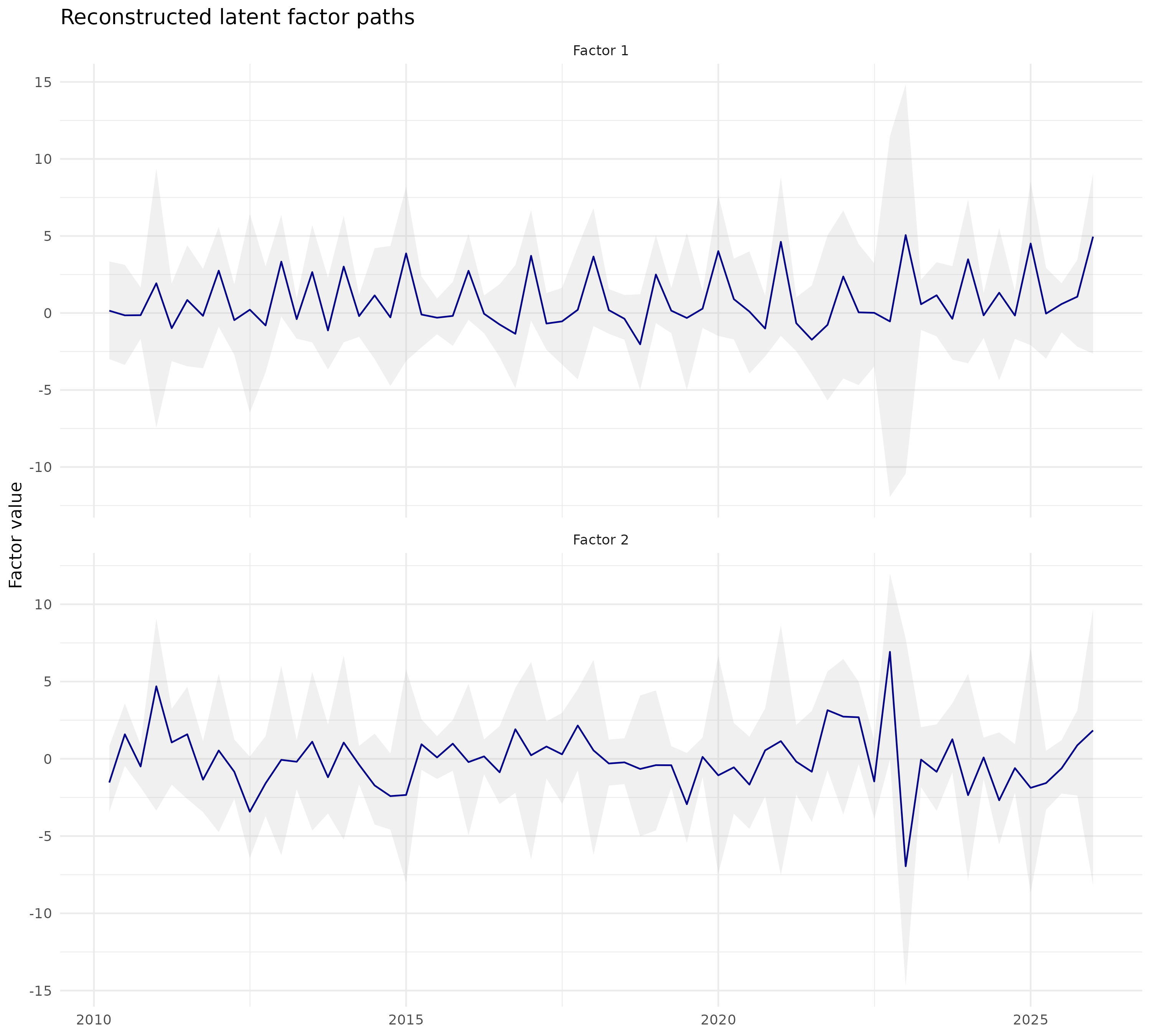
Figure 4 plots the posterior mean paths of together with 95% credible intervals. Both factors exhibit pronounced movements around 2022–2023, indicating a substantial common disturbance during that period. In addition, Factor 1 displays a clear recurrent pattern at roughly annual frequency, suggesting that some seasonal or other within-year variation may remain even after transformation. More broadly, both factor paths show short-run oscillations, although this feature is especially pronounced for Factor 1.
Overall, the Korean macroeconomic dataset exhibits a moderate common component, although its strength varies across variable groups. The common signal appears most clearly in interest-rate variables, while other categories show a more heterogeneous mix of common and idiosyncratic variation. Under the current specification with differenced and standardized quarterly variables, the factor paths are primarily useful for summarizing short-run common movements.
7 Conclusion
We introduce a novel Bayesian framework for approximate factor models. By placing priors directly on the eigenstructure of the common component, we address rotational non-identifiability while enabling accurate recovery of the factor subspace and associated eigenvalues. We derive posterior contraction rates for the leading eigenvalues and eigenspace, providing a theoretical foundation for the proposed procedure. Our simulation results confirm improved recovery of the underlying eigenstructure, particularly under relative error metrics. Furthermore, in real data analyses, the proposed method yields interpretable estimates of the common factor structure and delivers competitive forecasting performance at medium to long horizons in a factor-augmented VAR exercise, relative to standard shrinkage and PCA-based approaches. Extending the framework to dynamic factor models with time-varying eigenstructures is a promising direction for future research.
Acknowledgements
Seongmin Kim was supported by Global - Learning & Academic research institution for Master’s·PhD students, and Postdocs(G-LAMP) Program of the National Research Foundation of Korea(NRF) grant funded by the Ministry of Education(No. RS-2025-25442252). Jaeyong Lee was supported by the National Research Foundation of Korea (NRF) grant funded by the Korea government (MSIT) (No. 2023R1A2C1003050 and RS-2024-00406127).
References
- Bayesian dynamic factor models and portfolio allocation. Journal of Business & Economic Statistics 18 (3), pp. 338–357. Cited by: §6.3.
- Efficient estimation of approximate factor models via penalized maximum likelihood. Journal of econometrics 191 (1), pp. 1–18. Cited by: §5, §6.2.
- Determining the number of factors in approximate factor models. Econometrica 70 (1), pp. 191–221. Cited by: §1, §6.1, §6.2, §6.3.
- Inferential theory for factor models of large dimensions. Econometrica 71 (1), pp. 135–171. Cited by: §1.
- Measuring the effects of monetary policy: a factor-augmented vector autoregressive (favar) approach. The Quarterly journal of economics 120 (1), pp. 387–422. Cited by: §1, §6.2.
- Sparse bayesian infinite factor models. Biometrika 98 (2), pp. 291–306. Cited by: §1.
- Limiting laws for divergent spiked eigenvalues and largest nonspiked eigenvalue of sample covariance matrices. The Annals of Statistics 48 (3), pp. 1255–1280. Cited by: §1.
- ARBITRAGE, factor structure, and mean-variance analysis on large asset markets. Econometrica (pre-1986) 51 (5), pp. 1281. Cited by: §1.
- The rotation of eigenvectors by a perturbation. iii. SIAM Journal on Numerical Analysis 7 (1), pp. 1–46. Cited by: §2.3.
- Common risk factors in the returns on stocks and bonds. Journal of financial economics 33 (1), pp. 3–56. Cited by: §1.
- Large covariance estimation by thresholding principal orthogonal complements. Journal of the Royal Statistical Society Series B: Statistical Methodology 75 (4), pp. 603–680. Cited by: §1.
- The generalized dynamic-factor model: identification and estimation. Review of Economics and statistics 82 (4), pp. 540–554. Cited by: §1, §6.3.2.
- Data library. Note: http://mba.tuck.dartmouth.edu/pages/faculty/ken.french/data_library.htmlAccessed: 2025-11-12 Cited by: §6.2.
- Matrix analysis. Cambridge university press. Cited by: §2.3.
- On the distribution of the largest eigenvalue in principal components analysis. The Annals of statistics 29 (2), pp. 295–327. Cited by: §1.
- Eigenstructure inference for high-dimensional covariance with generalized shrinkage inverse-wishart prior. arXiv preprint arXiv:2505.20668. Cited by: §1, §4, §4, §4, §5.
- BVAR: bayesian vector autoregressions with hierarchical prior selection in r. Journal of Statistical Software 100, pp. 1–27. Cited by: §6.2, §6.2.
- Bayesian analysis of spiked covariance models: correcting eigenvalue bias and determining the number of spikes. arXiv preprint arXiv:2412.10753. Cited by: §1.
- Bayesian model assessment in factor analysis. Statistica Sinica, pp. 41–67. Cited by: §1.
- FRED-qd: a quarterly database for macroeconomic research. Technical report National Bureau of Economic Research. Cited by: §6.2.
- Slice sampling. The annals of statistics 31 (3), pp. 705–767. Cited by: item Step II., item 1.
- The arbitrage theory of capital asset pricing. Journal of Economic Theory 13 (3), pp. 341–360. External Links: Document, Link Cited by: §1.
- Dynamic factor models, factor-augmented vector autoregressions, and structural vector autoregressions in macroeconomics. In Handbook of macroeconomics, Vol. 2, pp. 415–525. Cited by: §6.3.2.
- Multiple factor analysis.. Psychological review 38 (5), pp. 406. Cited by: §6.3.1.
- Asymptotics of empirical eigenstructure for high dimensional spiked covariance. Annals of statistics 45 (3), pp. 1342. Cited by: §1, §1, §4, §4, §4, §5, §6.2.