The algorithm accepts input data with detector voltage bias, anomalous pixels, dark current, and radiation contributions removed. The algorithm first divides the image into a grid of $10$ concentric radial bins and $12$ angular bins, yielding a set of curvilinear bins of pixels over which statistics can be computed. The algorithm then repeats the following in an iterative manner:

1. 1.

   For each bin, the median pixel value is calculated, excluding any NaN entries. These local medians are then projected back onto the image coordinate system to construct a spatial background estimate.

2. 2.

   The background estimate is subtracted from the original image to generate a ‘demeaned’ image. In this residual frame, stellar sources appear as positive bright outliers against a zero-centered noise floor.

3. 3.

   The variance of the ‘demeaned’ pixels is calculated within each bin. These local variance values are subsequently mapped back to the full resolution of the original image grid.

4. 4.

   Negative values in the ‘demeaned’ image are clamped to zero, and a proxy Signal-to-Noise Ratio (SNR) is derived by dividing the square of the pixel value by the local variance. Pixels exceeding a defined SNR threshold–empirically established at $25$–are identified as candidate stars. To account for flux distribution across the Point Spread Function (PSF), these detection points are dilated circularly.

5. 5.

   Identified star pixels are accumulated into a global mask and set to NaN in the data to preclude re-detection. The algorithm iterates until convergence is achieved (defined as no change in the mask between steps) or a maximum of five iterations is reached.

Validation of the stellar location retrieval algorithm utilizes the numerical image simulator to generate a single instrument-effect-corrected image on the WFI channel targeting a star in the calibration stellar target database. Figure 2(a) displays the calibrated image cropped to the region of interest surrounding the target star. The full image is then processed by the stellar location retrieval algorithm. Figure 2(b) displays the same calibrated image cropped to the same region of interest, with pixels returned by the stellar location retrieval algorithm set to zero. The two figures show that any pixels contaminated by the star have been masked; the signal remaining in the images is from other photon backgrounds.

Data voids with a total area exceeding an empirically derived threshold of $\sim 250$ pixels are preserved, while smaller gaps undergo interpolation. The reconstruction utilizes the Radial Basis Function (RBF) interpolator provided by the scipy.interpolate package [17]. The interpolation is constrained to the nearest $100$ neighboring pixels and incorporates a third-degree polynomial into the basis to mitigate overfitting to noise.

The validation of this algorithm extends the analysis presented in Section 3. The masked image (Figure 3(a)) was processed using the interpolation algorithm. As demonstrated in Figure 3(b), the masked pixels were repopulated with values consistent with the surrounding background, effectively excising the stellar source from the image.

The relative responsivity retrieval algorithm is applied to raw images after all instrument backgrounds are removed. Additionally, all stars, the Moon, and any outer planets present in the image are masked, since these introduce non-Ly-$\alpha$ sources of photons. Finally, images pointed at Earth nadir have a circle with radius that corresponds to $2R_{E}$ on the image plane masked, since pixels within this radius in these images are contaminated by Out-Of-Band emission from Earth’s atmosphere, which is also a non-Ly-$\alpha$ source of photons. Here, $1R_{E}\approx 6371$km, or one Earth-radii. The boundary of $2R_{E}$ is conservative; the NFI’s field-of-view extends to $\sim 7.4R_{E}$ (and WFI’s field-of-view extends to $\sim 35R_{E}$); therefore, excluding the pixels within $2R_{E}$ removes a negligible fraction of the total observational area, preserving the vast majority of the data for the retrieval.

The relative Ly-$\alpha$ responsivity retrieval algorithm involves taking a ratio of the average signal rate [DN/s] measured in two images of the same scene using two different channel/filter combinations. The average signal rate, in [DN/s], is calculated over all non-masked pixels in the FOV of the two images. The different sizes of the FOV must be considered when recovering relative responsivity across different channels; in this case, only WFI pixels measuring regions of the scene that are also covered by NFI are used in the calculation of signal rate, in [DN/s], for the WFI image. These retrieved relative Ly-$\alpha$ responsivity factors are archived by the Carruthers mission as part of the CAL_XFACT calibration data product.

The algorithm was validated using the numerical image simulator to generate a set of $500$ instrument-effect-corrected images for each channel using the open and LyaN filters pointed at Earth nadir, each with an integration time of $30$ minutes (or $14400$ frames), which corresponds to the baseline image acquisition scheme on-orbit. Additionally, the stars, the Moon, and the outer planets were masked out. Pairs of calibrated images are then processed through the relative Ly-$\alpha$ responsivity retrieval algorithm and the result is compared to the ground-truth relative Ly-$\alpha$ responsivity. It was found that the retrieval algorithm performs well, with the percent error statistics having a negligible mean and a low standard deviation of $0.25\%$. This algorithm is much more accurate compared to the absolute responsivity algorithm because the final relative responsivity is a ratio of two averages, each of which are the average over $\sim 700,000$ Gaussian-distributed independent pixels for any NFI image and over $\sim 10,000$ Gaussian-distributed independent pixels for any WFI image. The SNR of these measured averages is incredibly high, leading to a precise and accurate measurement of the relative responsivity ratio at Ly-$\alpha$.

The IPH map retrieval algorithm processes L1B images from both channels, restricted to the open, LyaN, and LyaX filters. Prior to ingestion, celestial sources such as the stars, the Moon, and the outer planets are either masked or interpolated using the algorithm described in Section 5. The algorithm assumes that the relative Ly-$\alpha$ responsivity between each channel/filter combination and the WFI LyaN channel/filter combination is known, since the IPH map is defined in terms of observations from the WFI LyaN channel/filter combination. Details on the relative Ly-$\alpha$ responsivity retrieval algorithm can be found in Section 6; for this section, it suffices to recall that this algorithm is very accurate.

The IPH map is constructed using Heliocentric Mean Ecliptic latitude and longitude coordinates at a $0.2^{\circ}\times 0.2^{\circ}$ resolution. Any images that are off-nadir will measure IPH and are thus ingested into the IPH map retrieval algorithm. Finally, the IPH is measured in the outer annulus of every WFI image pointed at nadir. The inner boundary of the annulus to be used is 25 Earth-Radii ($R_{E}$) from the location of the Earth on the image plane: the IPH signal in pixels within this inner boundary are obfuscated by the Earth and its exosphere. A radius of $25R_{E}$ is selected because the Zoenchenn ground-truth model for Hydrogen 3D density predicts that the Ly-$\alpha$ radiance from the exosphere is around $3.33\times 10^{5}\pm 0.44\times 10^{5}$ [photon/s/cm²] at an altitude of $25R_{E}$ [20], which is negligible (about 1%) compared to the IPH’s minimum radiance of $\sim 3.18\times 10^{7}$ [photon/s/cm²]. The plate scale of the image is calculated based on the known camera viewing geometry to determine which pixels in the WFI image are ingested in the IPH map retrieval algorithm.

A corresponding IPH measurement time map is also constructed in parallel with the IPH map, with the same resolution in the same coordinate system. This map stores the total measurement time each pixel of the IPH map has received, in units of seconds.

To update the IPH and measurement time maps, the algorithm begins by normalizing input images by the solar Ly-$\alpha$ flux and the WFI LyaN cross-calibration factor. Relevant pixels are then extracted and spatially downsampled to the IPH map resolution via linear interpolation. Data integration follows a time-weighted averaging scheme: if a map pixel is unpopulated, the new measurement is weighted by its integration time and stored. Conversely, if a pixel contains existing data, the algorithm retrieves the stored value, reconstructs the total integrated signal, adds the new time-weighted measurement, and renormalizes by the updated total integration time. This process yields a cumulative average intensity for each pixel while explicitly updating the corresponding measurement time map.

The final IPH map will be in units of [DN/sec / ($10^{11}$ phot/sec/$\text{cm}^{2}$)], with the $10^{11}$ factor removed to keep the map numerically stable. The [DN] in these units specifically refer to [DN] as measured by the WFI LyaN channel/filter combination. The final IPH measurement map will have units of [sec]. These retrieved IPH map and IPH measurement maps are archived by the Carruthers mission as part of the CAL_IPH calibration data product.

The validation of the IPH map construction algorithm relied on a manually constructed, semi-realistic observation schedule designed to emulate mission conditions. The timeline encompasses the science commissioning phase (November 7th, 2025 to January 1st, 2026), featuring $80$ stellar targets for initial responsivity calibration, followed by nominal science operations extending through November 7th, 2026. The schedule incorporates $11$ flat-field and $70$ stellar acquisitions distributed throughout the period after January 1st, 2026, with the remaining image time allocated to nadir observations. All synthetic instrument-effect-corrected images were generated using the numerical image simulator described in Filippini et al. (2026) [4], incorporating realistic noise profiles derived from synthetic Carruthers L2 solar Ly-$\alpha$ flux data. Celestial sources such as the stars, the Moon, and the outer planets are either masked or interpolated using the algorithm described in Section 5.

Figure 5 presents the reconstructed IPH map following one year of semi-realistic science operations. The map exhibits heterogeneous noise levels correlated with observation type: regions associated with stellar targets show higher variance due to the short integration times characteristic of these observations. In contrast, the concentric rings in the center, derived from WFI nadir annuli, represent the smoothest portions of the dataset, reflecting the large amount of time allocated to nadir pointing. The corresponding spatial distribution of total integration time is illustrated in Figure 6.

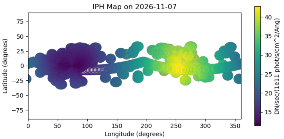
The discrete annular structures visible in the IPH map and measurement time map are artifacts of the validation protocol rather than physical features. These discontinuities arise from downsampling the spacecraft ephemeris and viewing geometry to a daily resolution to reduce computational load; operational on-orbit maps will show a spatially smoother distribution. It was found that the percent error magnitude remains negligible across the majority of the field, with elevated deviations confined to regions of low integration time, which is consistent with statistical expectations.

Utilizing the IPH map constructed in the previous section (accessible via the CAL_IPH data product), the contribution of IPH photons, in units of [DN], in science images is determined through a systematic scaling and fitting process. First, the map is renormalized by the most recent available solar Ly-$\alpha$ flux measurement and the WFI LyaN cross-calibration factor (from the CAL_XFACT data product). The map is then linearly interpolated to match the target image coordinates. Finally, to mitigate noise and bridge coverage gaps in unsampled regions, a weighted 2D polynomial fit is applied to derive the final IPH signal contribution in [DN/s]. This fit utilizes an order $3$ polynomial for WFI images and order $2$ for NFI images. The fitting weights are derived from the IPH measurement time map, ensuring that pixels representing longer integration time, and thus higher statistical reliability, are prioritized.

The IPH interpolation algorithm was validated by using the numerical image simulator to generate a raw LyaN image on each channel. The LyaN image had an integration time of $30$ minutes for NFI and $60$ minutes for WFI, designed to mimic the nominal parameters of planned nadir-pointed science observations. These simulated L0 images were processed through all instrument effect corrections described in Zhang et al. (2026) [10], with supporting images generated using the numerical image simulator as necessary. Finally, the stars, the Moon, and the outer planets are masked out or interpolated. The resulting calibrated images were then processed by the IPH retrieval algorithm. The mean percent error on the retrieved IPH signal was found to be $-0.13\%$ and $0.4\%$ for the NFI and WFI channels respectively, while the standard deviation is found to be below $1.4\%$ for both channels. Both the mean bias and the standard deviation fall well within $30\%$, which indicates that the IPH map construction and IPH removal algorithms algorithm meet the $30\%$ accuracy requirement mandated by NASA.

The deblurring algorithm uses a variation of the plug-and-play framework described in Venkatakrishnan et al. (2013) [16]. Unlike classical deconvolution, the plug-and-play framework uses denoising algorithms as a prior for the final image rather than applying standard regularization methods like Tikhonov regularization. A Wavelet-based thresholding technique is used for denoising in the deblurring algorithm presented in this section. Let $\vec{y}$ represent the image to be deblurred and $\boldsymbol{H}$ represent the linear operator that convolves input $\vec{x}$ with the PSF $h(i,j)$. The deblurring algorithm initializes $\vec{x}_{0}$ and $\vec{z}_{0}$ to zero, subsequently executing approximately 40 iterations of the following update sequence:

1. 1.

   $\vec{x}_{k}=\underset{\vec{x}}{\operatorname*{arg\,min}}\|\vec{y}-\boldsymbol{H}\vec{x}\|_{2}^{2}+\gamma_{1}\|\vec{x}-\vec{z}_{k-1}\|_{2}^{2}$

2. 2.

   $\vec{z}_{k}=\text{WaveletDenoiser}(\vec{x}_{k},\frac{\gamma_{2}}{\gamma_{1}})$

In this formulation, $\gamma_{1}$ and $\gamma_{2}$ serve as tunable hyperparameters governing algorithmic convergence, with the final deblurred output denoted as $\vec{x}_{40}$. The minimization step for $\vec{x}_{k}$ is solved numerically via gradient descent utilizing the ADAM optimizer [7]. To maximize computational efficiency through parallelization, the algorithm is implemented in PyTorch [12].

As the primary objective of the deblurring algorithm is to minimize error in the OOB photon background retrieval, the algorithm is not validated in isolation. Instead, its performance is assessed as an integrated component of the OOB retrieval pipeline in the next section.

The Out-of-Band (OOB) retrieval algorithm processes $30$-minute exposures of a static scene on the NFI channel, utilizing the filter sequence and image stacking protocol described previously. Input images require extensive preprocessing: instrument effects must be corrected (see Zhang et al. (2026) [10] for details), IPH photon backgrounds must be removed (see Section 7), stellar sources must be interpolated (see Section 5), and the Moon and outer planets must be masked (see Section 4). Furthermore, the algorithm relies on knowledge of absolute responsivities, $r_{f}(\lambda)$, for all filters at the $1216$Å, $1304$Å, and $1356$Å emission lines (see Zhang et al. (2026) [19] for details).

The mean of each pixel in the FOV for non-blocked images was derived Filippini et al. (2026) [4]. Removing instrument effects and expanding yields the following expression:

$$\mathbb{E}\left[S_{\text{FOV, OOB input},f}(p,q)\right]=\sum_{k=1}^{n_{\text{frame}}}\sum_{i=pn_{\text{bin}}}^{(p+1)n_{\text{bin}}-1}\sum_{j=qn_{\text{bin}}}^{(q+1)n_{\text{bin}}-1}g_{\text{adc}}\mathbb{E}[G_{\text{mcp}}]\frac{a\Omega}{4\pi}\\ \int_{t_{k}}^{t_{k}+t_{\text{frame}}}\int\varepsilon(\lambda)\tau_{f}(\lambda)(\ell(\lambda,i,j,t)*h(i,j))d\lambda dt$$

Next, the scene model described in Filippini et al. (2026) [4] can be substituted for $\ell(\lambda,i,j,t)$. Since IPH, stars, the Moon, and the outer planets have already been removed, the only two terms remaining in $\ell(\lambda,i,j,t)$ are $\ell_{\text{exo}}(\lambda,i,j,t)$ and $\ell_{\text{OOB}}(\lambda,i,j,t)$. For analytical convenience, the constituent terms are consolidated and subsequently re-partitioned into two new terms. The first term isolates the discrete line emissions (H1216, O1304, and O1356), characterized by Dirac delta distributions in wavelength. This component is explicitly expanded as a summation indexed by $m$. The second term, representing the remaining non-discrete sources, is aggregated into the background spectral radiance $\ell_{\text{bkgd}}(\lambda,i,j,t)$.

$$\mathbb{E}\left[S_{\text{FOV, OOB input},f}(p,q)\right]=\sum_{k=1}^{n_{\text{frame}}}\sum_{i=pn_{\text{bin}}}^{(p+1)n_{\text{bin}}-1}\sum_{j=qn_{\text{bin}}}^{(q+1)n_{\text{bin}}-1}g_{\text{adc}}\mathbb{E}[G_{\text{mcp}}]\frac{a\Omega}{4\pi}\\ \int_{t_{k}}^{t_{k}+t_{\text{frame}}}\int\varepsilon(\lambda)\tau_{f}(\lambda)\left(\left[\sum_{m}i_{m}(i,j,t)\delta(\lambda-\lambda_{m})+\ell_{\text{bkgd}}(\lambda,i,j,t)\right]*h(i,j)\right)d\lambda dt$$

The summation over $n_{\text{frame}}$ image frames and the integration over time over the time-dependent terms can be replaced by a multiplication of $t_{\text{int},f}$ (the integration time of the image taken with filter $f$) with the time-average of the terms that depend on $t$, which is denoted as $\bar{i}_{m}(i,j)$ and $\bar{\ell}_{\text{bkgd}}(\lambda,i,j)$.

$$\mathbb{E}\left[S_{\text{FOV, OOB input},f}(p,q)\right]=\sum_{i=pn_{\text{bin}}}^{(p+1)n_{\text{bin}}-1}\sum_{j=qn_{\text{bin}}}^{(q+1)n_{\text{bin}}-1}g_{\text{adc}}\mathbb{E}[G_{\text{mcp}}]\frac{a\Omega}{4\pi}t_{\text{int},f}\\ \int\varepsilon(\lambda)\tau_{f}(\lambda)\left(\left[\sum_{m}\bar{i}_{m}(i,j)\delta(\lambda-\lambda_{m})+\bar{\ell}_{\text{bkgd}}(\lambda,i,j)\right]*h(i,j)\right)d\lambda$$

The integration over $\lambda$ can be split into two pieces.

$$\mathbb{E}\left[S_{\text{FOV, OOB input},f}(p,q)\right]=\\ \sum_{i=pn_{\text{bin}}}^{(p+1)n_{\text{bin}}-1}\sum_{j=qn_{\text{bin}}}^{(q+1)n_{\text{bin}}-1}g_{\text{adc}}\mathbb{E}[G_{\text{mcp}}]\frac{a\Omega}{4\pi}t_{\text{int},f}\int\varepsilon(\lambda)\tau_{f}(\lambda)\left[\sum_{m}\bar{i}_{m}(i,j)\delta(\lambda-\lambda_{m})\right]*h(i,j)d\lambda\\ +\sum_{i=pn_{\text{bin}}}^{(p+1)n_{\text{bin}}-1}\sum_{j=qn_{\text{bin}}}^{(q+1)n_{\text{bin}}-1}g_{\text{adc}}\mathbb{E}[G_{\text{mcp}}]\frac{a\Omega}{4\pi}t_{\text{int},f}\int\varepsilon(\lambda)\tau_{f}(\lambda)\bar{\ell}_{\text{bkgd}}(\lambda,i,j)*h(i,j)d\lambda$$

The first term is an integral over the summation of Dirac delta distributions and can be simplified. The definition of $r_{f}(\lambda)$ from Zhang et al. (2026) [19] can also be plugged in.

$$\mathbb{E}\left[S_{\text{FOV, OOB input},f}(p,q)\right]=\sum_{i=pn_{\text{bin}}}^{(p+1)n_{\text{bin}}-1}\sum_{j=qn_{\text{bin}}}^{(q+1)n_{\text{bin}}-1}\sum_{m}g_{\text{adc}}\mathbb{E}[G_{\text{mcp}}]\frac{a\Omega}{4\pi}t_{\text{int},f}r_{f}(\lambda_{m})\bar{i}_{m}(i,j)*h(i,j)d\lambda\\ +\sum_{i=pn_{\text{bin}}}^{(p+1)n_{\text{bin}}-1}\sum_{j=qn_{\text{bin}}}^{(q+1)n_{\text{bin}}-1}g_{\text{adc}}\mathbb{E}[G_{\text{mcp}}]\frac{a\Omega}{4\pi}t_{\text{int},f}\int r_{f}(\lambda)\bar{\ell}_{\text{bkgd}}(\lambda,i,j)*h(i,j)d\lambda$$

The above equation is valid for each filter $f$. The four equations for the four filters can be stacked to yield a matrix equation:

$$\begin{bmatrix}\mathbb{E}\left[S_{\text{FOV, OOB input},f_{1}}(p,q)\right]\\ \vdots\\ \mathbb{E}\left[S_{\text{FOV, OOB input},f_{4}}(p,q)\right]\end{bmatrix}=\sum_{i=pn_{\text{bin}}}^{(p+1)n_{\text{bin}}-1}\sum_{j=qn_{\text{bin}}}^{(q+1)n_{\text{bin}}-1}g_{\text{adc}}\mathbb{E}[G_{\text{mcp}}]\frac{a\Omega}{4\pi}\\ \begin{bmatrix}t_{\text{int},f_{1}}r_{f_{1}}(1216)&t_{\text{int},f_{1}}r_{f_{1}}(1304)&t_{\text{int},f_{1}}r_{f_{1}}(1356)\\ \vdots&\ddots&\vdots\\ t_{\text{int},f_{4}}r_{f_{4}}(1216)&t_{\text{int},f_{4}}r_{f_{4}}(1304)&t_{\text{int},f_{4}}r_{f_{4}}(1356)\\ \end{bmatrix}\begin{bmatrix}\bar{i}_{\text{H1216}}(i,j)*h(i,j)\\ \bar{i}_{\text{O1304}}(i,j)*h(i,j)\\ \bar{i}_{\text{O1356}}(i,j)*h(i,j)\end{bmatrix}\\ +\sum_{i=pn_{\text{bin}}}^{(p+1)n_{\text{bin}}-1}\sum_{j=qn_{\text{bin}}}^{(q+1)n_{\text{bin}}-1}g_{\text{adc}}\mathbb{E}[G_{\text{mcp}}]\frac{a\Omega}{4\pi}\begin{bmatrix}\int r_{f_{1}}(\lambda)\bar{\ell}_{\text{bkgd}}(\lambda,i,j)*h(i,j)d\lambda\\ \vdots\\ \int r_{f_{4}}(\lambda)\bar{\ell}_{\text{bkgd}}(\lambda,i,j)*h(i,j)d\lambda\end{bmatrix}$$

In the on-orbit operational environment, the theoretical expected value on the left-hand side is inaccessible; consequently, it is replaced by the stochastic measurement vector, denoted as $\vec{Y}(p,q)$. The right-hand side can be simplified by introducing some notation:

$$\vec{Y}(p,q)=\sum_{i=pn_{\text{bin}}}^{(p+1)n_{\text{bin}}-1}\sum_{j=qn_{\text{bin}}}^{(q+1)n_{\text{bin}}-1}g_{\text{adc}}\mathbb{E}[G_{\text{mcp}}]\frac{a\Omega}{4\pi}\left(\boldsymbol{R}\vec{x}(i,j)+\vec{z}(i,j)\right)$$

The binning operation can be written as another linear operator $\boldsymbol{B}$:

$$\vec{Y}(p,q)=g_{\text{adc}}\mathbb{E}[G_{\text{mcp}}]\frac{a\Omega}{4\pi}\boldsymbol{B}\left(\boldsymbol{R}\vec{x}(i,j)+\vec{z}(i,j)\right)$$

The above only describes a single binned pixel $p,q$. Equations for all the binned pixels can be combined into a single equation by adding more columns to $\vec{x}$, $\vec{z}$, and $\vec{Y}$, thus turning them into matrices.

$$\boldsymbol{Y}=g_{\text{adc}}\mathbb{E}[G_{\text{mcp}}]\frac{a\Omega}{4\pi}\boldsymbol{B}\left(\boldsymbol{R}\boldsymbol{X}+\boldsymbol{Z}\right)$$

(1)

The algorithmic objective is to solve for $\boldsymbol{X}$ and $\boldsymbol{Z}$ utilizing the noisy measurement vector $\boldsymbol{Y}$ and the responsivity matrix $\boldsymbol{R}$ (derived via the responsivity retrieval algorithm detailed in Zhang et al. (2026) [19]). However, the inclusion of the $\boldsymbol{Z}$ term renders the system underdetermined, thereby precluding the use of standard least-squares minimization. Consequently, to reach a unique solution, it is necessary to impose specific physical constraints on $\boldsymbol{X}$ and $\boldsymbol{Z}$.

The structure that the solution $\boldsymbol{X}$ should take can be found by examining the original scene model for OOB photons found in Filippini et al. (2026) [4]. Since the set of pixels $\boldsymbol{J}$ where OOB characterization is required is in the range $1.078<r_{ij}<1.4$, which is completely within $1.055<r_{ij}<1.5$, $\boldsymbol{X}$ should take the form of a summation of three exponential decays as a function of radius, with one exponential decay for each line emission. Recall the mapping from APS pixel $i,j$ to pixel indices $p_{ij},q_{ij}$, where the latter are the pixel indices of the closest in the set of pixels $\boldsymbol{D}$ that satisfy $r_{p_{ij}q_{ij}}<1$. The algorithm therefore imposes a constraint where all channel pixels $i,j$ that map to the same pixel index $p_{ij},q_{ij}$ are part of the same set of three exponential decays. Thus, each of these sets comes with six unknowns: three amplitudes $\beta_{m}[p_{ij},q_{ij}]$ and three decay rates $\alpha_{m}[p_{ij},q_{ij}]$. Unfortunately, radial exponentials are expected to change shape drastically under 2D blurring by the instrument PSF. Thus, the images $\boldsymbol{Y}$ are first deblurred using the algorithm described in Section 8. Ideally, this removes all instances of $h(i,j)$ from Equation 1 and increases modeling accuracy.

The background $\boldsymbol{Z}$ has three components: two LBH emissions, which yield a relatively weak [DN] contribution due to the instrument’s low responsivity at these wavelengths for all filters, and the Earth continuum albedo, which is only present due to blur. Therefore, minimal error is incurred if the algorithm assumes that $\boldsymbol{Z}$ must follow the shape of a blurred Earth’s disk that is then deblurred. Let this scaling factor be a column vector denoted $\vec{s}_{\text{bkgd}}(i,j)$. Thus, the $4\|\boldsymbol{J}\|$ unknowns in $\boldsymbol{Z}$ have been reduced to only $4$ unknowns: one amplitude $\beta_{\text{bkgd},f}$ corresponding to the solar continuum albedo for each filter $f$. Let the four amplitudes be rewritten into a single vector $\vec{\beta}_{\text{bkgd}}=\begin{bmatrix}\beta_{\text{bkgd},f_{1}},&\cdots,&\beta_{\text{bkgd},f_{4}}\\ \end{bmatrix}^{T}$. Assuming no noise, a perfect model, negligible contributions from LBH, and a perfect deblurring algorithm, $\boldsymbol{Z}$ can then be written as $\boldsymbol{Z}=\vec{\beta}_{\text{bkgd}}\vec{s}_{\text{bkgd}}^{T}$.

The final least-squares minimization is performed over the amplitudes and decay rates of all the line emission exponentials and the four unknown background amplitudes:

$$\operatorname*{arg\,min}_{\vec{\alpha},\vec{\beta},\vec{\beta}_{\text{bkgd}}}\left\|\text{deblur}\left(\boldsymbol{Y}\right)-\frac{a\Omega}{4\pi}\boldsymbol{B}\left(\boldsymbol{R}\boldsymbol{X}^{\prime}+\vec{\beta}_{\text{bkgd}}\vec{s}_{\text{bkgd}}^{T}\right)\right\|_{2}^{2}\\ \text{with }\boldsymbol{X}^{\prime}(i,j)=\begin{bmatrix}\beta_{\text{H1216}}[p_{ij},q_{ij}]\exp\left(\alpha_{\text{H1216}}[p_{ij},q_{ij}](r_{ij}-1)\right)\\ \vdots\\ \beta_{\text{O1356}}[p_{ij},q_{ij}]\exp\left(\alpha_{\text{O1356}}[p_{ij},q_{ij}](r_{ij}-1)\right)\\ \end{bmatrix}$$

The minimization is done numerically via Python’s scipy.optimize library [17]. Once $\vec{\alpha}$, $\vec{\beta}$, and $\vec{\beta}_{\text{bkgd}}$ are recovered, the final $\boldsymbol{X}$ and $\boldsymbol{Z}$ are reconstructed using

$$\boldsymbol{X}(i,j)=\begin{bmatrix}\beta_{\text{H1216}}[p_{ij},q_{ij}]\exp\left(\alpha_{\text{H1216}}[p_{ij},q_{ij}](r_{ij}-1)\right)\\ \vdots\\ \beta_{\text{O1356}}[p_{ij},q_{ij}]\exp\left(\alpha_{\text{O1356}}[p_{ij},q_{ij}](r_{ij}-1)\right)\\ \end{bmatrix}$$

$$\boldsymbol{Z}=\vec{\beta}_{\text{bkgd}}\vec{s}_{\text{bkgd}}^{T}$$

The last two rows of $\boldsymbol{X}$ represent the O1304 and O1356 radiances in units of [photons/cm²/s] in the altitude range 500-1500km, which is archived by the Carruthers mission as part of the CAL_OOB calibration data product. The four rows of $\boldsymbol{Z}$ represent the [DN] contribution for images taken by the four filters from all OOB photons that are not the three line emissions. These are also archived by the Carruthers mission as part of the CAL_OOB calibration data product.

The OOB removal algorithm proceeds by scaling the signal components from the CAL_OOB calibration product by the integration time of the input image, followed by subtraction. This correction is applied exclusively to the NFI pixel region of interest.

The OOB algorithm is validated by using the numerical image simulator to generate a sequence of four images on the NFI channel using four filters (open, LyaN, CaF₂, and SrF₂) with integration times of (30min, 60min, 30min, and 30min) respectively, followed by a 30-minute storm-time (S3) LyaN image on the NFI channel. Simulated L0 images were processed through the beginning of the calibration pipeline (instrument effect correction, star/Moon/outer planet masking and interpolation, IPH removal, and deblurring), with supporting images generated using the numerical image simulator as necessary. These images were then processed by the OOB retrieval algorithm described in this section.

Recall that this analysis focuses exclusively on the NFI channel within the region of interest defined by $1.078\text{R}_{\text{E}}<r_{ij}<1.428\text{R}_{\text{E}}$, where OOB contributions are actively recovered. In this region, the OOB intensity is typically a minor fraction of the total signal. Therefore, performance is validated relative to the target Ly-$\alpha$ signal; a larger relative error in the faint OOB component is permissible provided the absolute error magnitude remains negligible compared to the target Ly-$\alpha$ emission. The analysis yielded a mean error of $0.03\%$ with a standard deviation of $0.88\%$. These results are well within the $20\%$ requirement established by NASA, demonstrating the efficacy of the OOB retrieval and removal algorithm.

1. 1.

   Retrieve the locations of all stars in the image using the algorithm described in Section 3.

2. 2.

   Retrieve the locations of the Moon and the outer planets using the algorithm described in Section 4.

3. 3.

   Mask out all pixels that are a PSF-width away from the locations of the stars, the Moon, and the outer planets. Interpolate over smaller holes using the algorithm found in Section 5.

4. 4.

   Retrieve the cross-channel Ly-$\alpha$ responsivity ratio using the algorithm described in Section 6.

5. 5.

   Retrieve and subtract the mean [DN] contribution from IPH photons in the image using the algorithm found in Section 7.2.

6. 6.

   Deblur the image using the algorithm discussed in Section 8.

7. 7.

   If the image is from the NFI channel, subtract the most recent mean [DN] contribution from OOB photons from the calibration database.

8. 8.

   Divide by the corresponding absolute Ly-$\alpha$ responsivity to yield the L1C image in physical units of $\left[\frac{\text{ photons}}{\text{cm}^{2}\cdot\text{s}}\right]$.

The result of these operations are denoted L1C images. To validate the full L0 to L1C calibration pipeline, the numerical image simulator was utilized to generate synthetic L0 exposures for both channels. These simulations employed the baseline science filter (LyaN) and adopted integration times of $30$ minutes for NFI and $60$ minutes for WFI, designed to mimic the nominal parameters of planned nadir-pointed science observations. Other images (such as the flat-field set) are also generated as needed to support this test. It was found that the percent error on the ground-truth exospheric radiance is centered at $\boldsymbol{-2.9\%}$ with standard deviations on the order of $12.4\%$ for the NFI channel and $9.05\%$ for the WFI channel. While the deblurring algorithm introduces increased noise variance at the L1C stage relative to L1B, the overall accuracy remains exceptional. Both the mean and standard deviation of the percent error fall well within NASA’s $30\%$ threshold, showcasing just how far the calibration pipeline’s precision exceeds initial mission expectations.

References

- [1] (2019) SWAN/soho lyman- mapping: the hydrogen geocorona extends well beyond the moon. Journal of Geophysical Research: Space Physics 124 (2), pp. 861–885. External Links: Document Cited by: §1.
- [2] (1978) Interpretation of ogo-5 line shape measurements of lyman- emission from terrestrial exospheric hydrogen. Planetary and Space Science 26 (5), pp. 431–447. External Links: Document Cited by: §1.
- [3] (1976) Apollo 16 lyman alpha imagery of the hydrogen geocorona. Journal of Geophysical Research 81 (10), pp. 1664–1672. External Links: Document Cited by: §1.
- [4] (2026-02) Numerical Model Simulation of the Carruthurs Geocoronal Observatory. ssr 99999 (99999), pp. 0–0. External Links: Document Cited by: §1, §7.1, §9.1, §9.1, §9.1.
- [5] (1992) Space science reviews volume on galileo mission overview. Space Science Reviews 60 (1), pp. 3–21. External Links: Document Cited by: §1.
- [6] (2017) Ecliptic north-south symmetry of hydrogen geocorona. Geophysical Research Letters 44 (23), pp. 11–706. External Links: Document Cited by: §1.
- [7] (2017) Adam: a method for stochastic optimization. External Links: 1412.6980, Link Cited by: §8.1.
- [8] (1993) Deceleration of interstellar hydrogen at the heliospheric interface. Science 260 (5111), pp. 1095–1098. External Links: Document Cited by: §7.
- [9] (2008) Atmospheric escape and evolution of terrestrial planets and satellites. Space Science Reviews 139 (1), pp. 399–436. External Links: Document Cited by: §1.
- [10] (2026) On-orbit Calibration of the Carruthers GCI: Instrument Effect Correction. ssr. Note: Under review at Space Science Reviews Cited by: §1, §10, §7.2, §9.1.
- [11] (1991-12-01) Ultraviolet spectroscopy and remote sensing of the upper atmosphere. Space Science Reviews 58 (2). External Links: Document Cited by: §1.
- [12] (2019) PyTorch: an imperative style, high-performance deep learning library. 32, pp. . External Links: Link Cited by: §8.1.
- [13] (2013) Lyman- models for lro lamp from messenger mascs and soho swan data. In Cross-Calibration of Far UV Spectra of Solar System Objects and the Heliosphere, E. Quémerais, M. Snow, and R. Bonnet (Eds.), pp. 163–175. External Links: ISBN 978-1-4614-6384-9, Document, Link Cited by: Figure 4, Figure 4.
- [14] (2017) Redistribution of h atoms in the upper atmosphere during geomagnetic storms. Journal of Geophysical Research: Space Physics 122 (10), pp. 10–686. External Links: Document Cited by: §1.
- [15] (2026) Design and performance of the carruthers geocoronal imager. Note: Under review at Space Science Reviews Cited by: §4.
- [16] (2013) Plug-and-play priors for model based reconstruction. In 2013 IEEE Global Conference on Signal and Information Processing, Vol. , pp. 945–948. External Links: Document Cited by: §8.1.
- [17] (2020) SciPy 1.0: fundamental algorithms for scientific computing in python. Nature methods 17 (3), pp. 261–272. External Links: Document Cited by: §5.1, §9.1.
- [18] (2000) Improved solar lyman irradiance modeling from 1947 through 1999 based on uars observations. Journal of Geophysical Research: Space Physics 105 (A12), pp. 27195–27215. External Links: Document Cited by: §7.
- [19] (2026) On-orbit Calibration of the Carruthers GCI: Radiometric Sensitivity. ssr. Note: Under review at Space Science Reviews Cited by: §1, §10, §6, §9.1, §9.1, §9.1.
- [20] (2024) Comparison of terrestrial exospheric hydrogen 3d distributions at solar minimum and maximum using twins lyman-a observations. Frontiers in Astronomy and Space Sciences 11. External Links: Link, Document, ISSN 2296-987X Cited by: §7.1.