Testing Continuous Spontaneous Localization by Coherently Simulating a Measurement with a Nanoparticle
Abstract
We propose a direct Ramsey-interferometric test of Continuous Spontaneous Localization (CSL) in which a microscopic system controls the motion of a charged nanoparticle held in a harmonic trap. The microscopic system is prepared in a two-branch Ramsey superposition. During the Ramsey interval, the two branches exert opposite weak forces on the nanoparticle, so the nanoparticle center of mass follows two spatially separated trajectories. The procedure resembles a measurement: information about the microscopic branch is transferred to a mesoscopic object, but the transfer is then reversed coherently. After one period of the harmonic trap, the nanoparticle trajectories recombine in both position and momentum. The microscopic system is then measured through its final Ramsey visibility. Standard quantum mechanics predicts recovery of this visibility, while CSL predicts an irreversible visibility loss accumulated while the nanoparticle mass distributions were separated.
At the benchmark number of shots , the baseline polar-molecule and aggressive Rydberg-Stark operating points improve over digitized direct matter-wave CSL bounds by about and , respectively. These factors scale as , where is the number of shots. This improvement refers to direct interferometric CSL bounds; the projected sensitivities remain above the strongest non-interferometric CSL bounds, which probe different observables. Although the numerical reach is quoted in CSL parameters, the same visibility-loss measurement applies more broadly to collapse mechanisms that suppress spatial coherence.
I Introduction
Quantum theory provides a unitary description of microscopic systems, but ordinary measurements appear to produce definite outcomes. In the standard operational treatment this tension is hidden by the measurement postulate: microscopic systems evolve according to the Schrödinger equation until a measurement occurs, after which the state is updated nonunitarily. This division is practically successful, but it leaves open whether the apparent collapse of the quantum state is fundamental, emergent, or only an effective description of entanglement and decoherence. A related weak-measurement perspective on distinguishing collapse from purely unitary evolution is discussed in [1].
Objective-collapse models address this question by modifying quantum dynamics [2, 5, 6]. In these models, macroscopic spatial superpositions are dynamically suppressed by a stochastic physical process. Continuous Spontaneous Localization (CSL) is one of the most widely studied examples [3, 4, 6]. It introduces two phenomenological parameters: a collapse rate and a correlation length . For a mass distribution placed in a spatial superposition, CSL predicts an additional loss of coherence whose strength grows with mass and depends on the separation of the two mass distributions relative to . The experimental task is therefore to search for a visibility loss that cannot be explained by ordinary environmental decoherence.
A direct interferometric CSL test places a massive object in a spatial superposition and measures the survival of interference contrast [12, 13, 14]. This directly addresses whether coherence survives between spatially separated mass distributions, but producing large coherent separations for massive objects is experimentally demanding. The strongest overall CSL bounds therefore often come from non-interferometric observables, such as anomalous heating, force noise, spontaneous radiation, or related precision measurements [17, 18, 19, 20, 21, 22]. Those bounds strongly constrain CSL, but they infer the collapse parameters from secondary effects rather than from a direct visibility-loss measurement.
More broadly, a direct visibility-loss experiment is not limited to CSL. It is sensitive to any collapse mechanism that suppresses coherence between spatially separated mass distributions during the pointer separation, including CSL-like models and gravity-related Diósi-Penrose proposals [7, 8]. This broader relevance is one reason to emphasize the direct comparison class, even when model-specific heating, force-noise, or radiation bounds are numerically stronger for CSL.
Here we develop a direct Ramsey-interferometric route, sketched in Fig. 1. A microscopic system is prepared in a two-branch Ramsey superposition. During the Ramsey interval, the two branches exert opposite weak forces on a charged nanoparticle held in a harmonic trap. The nanoparticle center of mass then follows two spatially separated trajectories. The procedure resembles a measurement: information about the microscopic branch is transferred to a mesoscopic object, but the transfer is then reversed coherently. After one period of the harmonic trap, the two nanoparticle trajectories recombine in both position and momentum. The microscopic system is then measured through its final Ramsey visibility.
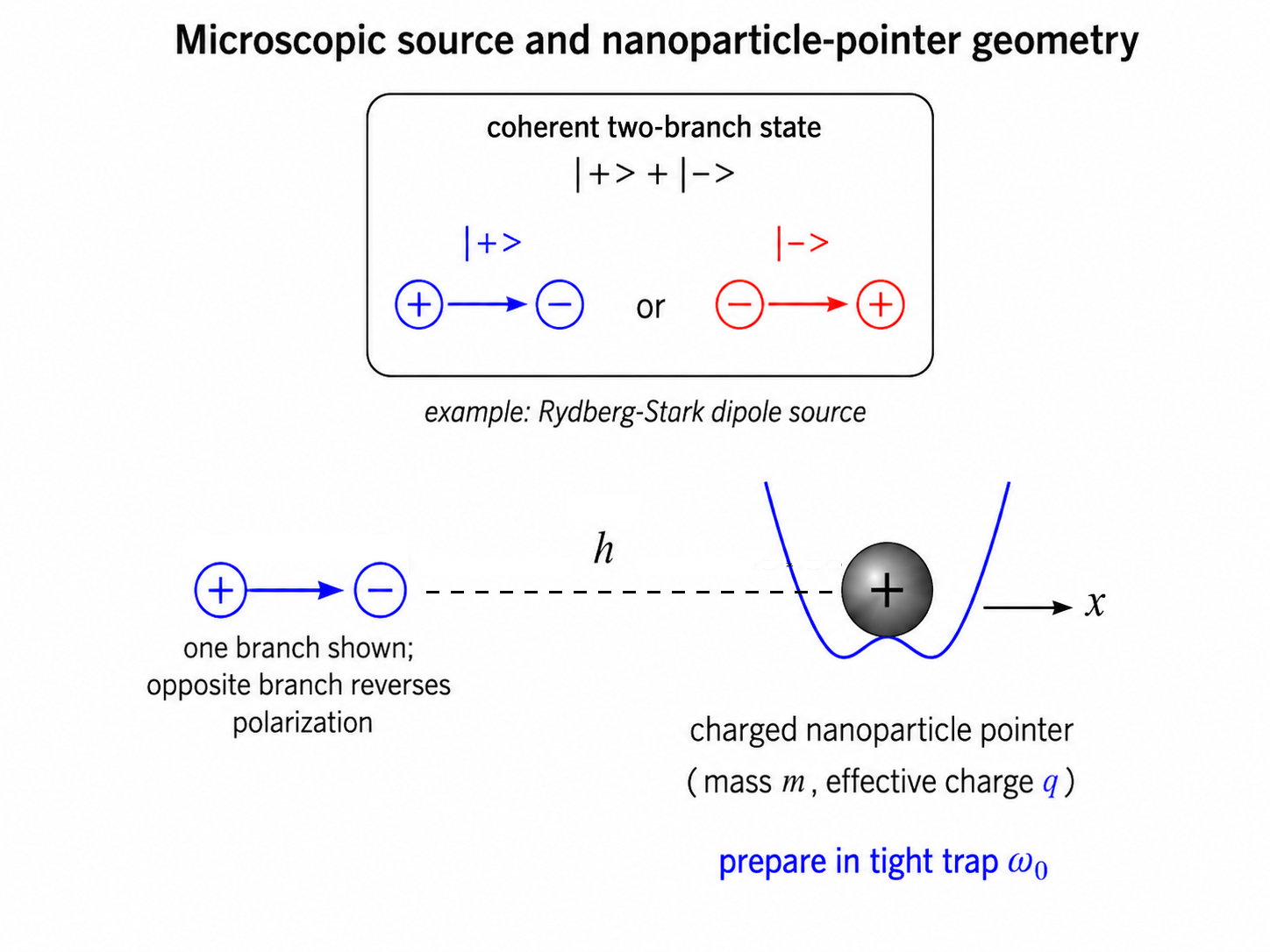
The figure shows the concrete source-pointer realization used for the estimates. The microscopic source is a coherent two-branch electric dipole. The two branches exert opposite forces on the nanoparticle along the trap axis. The source-pointer distance sets the force scale for the dipole-source estimate, and the nanoparticle parameters , , and set the pointer mass, effective charge, and initial preparation width. In the signal model we idealize this geometry as a branch-dependent constant force acting on a harmonic pointer. The source center of mass is assumed fixed by trapping in all three spatial directions; the two source branches differ by their internal dipole orientation, not by source motion. The nanoparticle is confined in the transverse directions and , so the modeled pointer coordinate is the axial displacement .
In standard quantum mechanics, the two nanoparticle trajectories close after one trap period. The which-branch information written into the nanoparticle is then erased, and the Ramsey visibility revives apart from technical and environmental imperfections. CSL, by contrast, acts during the temporary spatial separation of the nanoparticle mass distributions and produces an irreversible visibility loss that remains after recombination.
At intermediate times, the Ramsey coherence of the microscopic system alone cannot be separated from its entanglement with the nanoparticle. The protocol therefore measures the Ramsey visibility after one trap period, when standard quantum mechanics predicts that the nanoparticle has disentangled from the microscopic system.
This construction is related to earlier levitated-oscillator and trapped-nanosphere collapse tests. Romero-Isart analyzed collapse-model tests based on preparing and observing massive mechanical superpositions [15], while Goldwater, Paternostro, and Barker proposed a trapped-nanosphere test based on CSL-induced parametric heating [16]. The present protocol is closer to this hybrid source-oscillator family than to free matter-wave propagation, but its final observable is different: the nanoparticle temporarily carries branch information, and the measured quantity is the Ramsey visibility of the microscopic source after the nanoparticle trajectories have recombined.
The relevant CSL signal is the accumulated suppression of the off-diagonal density-matrix element associated with the two branch-conditioned nanoparticle states. For a sharply localized compact mass distribution and a branch separation , the small-separation CSL rate scales as
| (1) |
Here is the CSL collapse rate, is the nanoparticle mass, is the nucleon mass, is the CSL correlation length, and is the full separation between the two branch-conditioned nanoparticle centers. Thus the experiment can remain sensitive even when the realized pointer separation is much smaller than the CSL correlation length. Instead of requiring , it accumulates CSL-induced visibility loss from a controlled time-dependent branch separation with . The full CSL rate and the density-matrix derivation are given in Sec. II.
Equation (1) describes the idealized case in which the nanoparticle mass distribution is sharply localized. In the proposed experiment the nanoparticle has a finite wave-packet width, and this width changes during the weak-trap evolution. This effect must be included because CSL depends on the distinguishability of the two mass distributions. The nanoparticle is first prepared in a tight trap of frequency and then evolves in a weaker trap of frequency . At finite temperature the packet width breathes during the weak-trap evolution, which reduces the CSL distinguishability of the two mass distributions. Section II.6 derives this breathing correction and defines the suppression factor , the ratio of the breathing-corrected CSL signal to the ideal sharply localized signal. For the baseline operating point at , the conservative 3D-isotropic estimate gives . This is a conservative estimate because the actual branch separation is along one spatial direction, whereas the calculation below uses an isotropic 3D width.
The purpose of this paper is to quantify the viability of this coherent measurement-simulation test of CSL. We derive the CSL signal for the forced harmonic response, include thermal breathing, estimate ordinary visibility losses, and compute the number of experimental shots required for a detection. The number of shots is treated as an exposure parameter: we quote one benchmark value and give the rescaling with , rather than treating a single shot count as a platform-independent comparison. We focus on representative operating points rather than on a fully optimized design. The baseline point uses a polar-molecule-scale dipole, while the more aggressive point uses a Rydberg-Stark source. At , the baseline point gives
| (2) |
so the protocol operates deeply in the sub- regime. After including the breathing correction and an ordinary coherence-loss budget , with the electric-field and force-noise sub-budgets kept below , the projected point sensitivity at the benchmark exposure shots is
| (3) |
The aggressive point reaches below , at the cost of stronger technical requirements.
The remainder of the paper is organized as follows. Section II develops the density-matrix signal model, including the branch-conditioned mean response, endpoint Ramsey readout, CSL visibility loss, and thermal breathing correction. Section III discusses ordinary visibility losses, calibration effects, and the dominant feasibility requirements. Section IV presents the numerical sensitivity estimates. Section V compares the projected reach with existing CSL constraints.
II Signal model
II.1 Density-matrix description of the reversible pointer
We consider a microscopic quantum system coupled to the center-of-mass motion of a trapped nanoparticle. The nanoparticle acts as a reversible mesoscopic measurement pointer. During the interaction, the two microscopic branches exert opposite weak forces on the nanoparticle. The two branch-conditioned pointer means are then recombined, and the remaining microscopic coherence is read out interferometrically.
Let the microscopic system be prepared with density matrix
| (4) |
The nanoparticle pointer has center-of-mass coordinate , momentum , mass , and evolves in a harmonic trap of weak frequency . We define to be the differential force between the two microscopic branches. Thus the branch exerts force on the nanoparticle, while the branch exerts force . With this convention the conditional Hamiltonians are
| (5) |
The full density matrix can be written in branch-block form as
| (6) |
The diagonal blocks and describe the two branch-conditioned pointer states, while the off-diagonal block carries the microscopic coherence.
We write branch averages explicitly as
| (7) |
where the subscript or specifies which branch state is used for the average, and the trace is over the pointer Hilbert space. Ordinary unitary quantum mechanics predicts that, after a full weak-trap period, these branch averages recombine. CSL, by contrast, produces an irreversible suppression of the off-diagonal block associated with the two temporarily separated mass-density profiles.
II.2 Forced harmonic mean response
We assume that the two branch-conditioned pointer states begin with the same mean position and momentum,
| (8) |
The Ehrenfest equations for the two diagonal density-matrix blocks give
| (9) |
and
| (10) |
Therefore
| (11) |
and
| (12) |
We define the one-way mean displacement by
| (13) |
and the full branch separation by
| (14) |
The CSL formulas depend on , the full separation between the two branch-conditioned mass-density means.
The maximum one-way displacement occurs at half a weak-trap period, , and is
| (15) |
At one full weak-trap period,
| (16) |
the two branch averages recombine:
| (17) |
This exact harmonic recombination is central to the protocol. It allows the pointer to temporarily carry which-branch information and then coherently return that information to the microscopic system. Ordinary quantum mechanics therefore predicts recovery of the microscopic interference contrast, up to technical and environmental imperfections. CSL predicts an additional irreversible loss accumulated while the two branch-conditioned mass-density profiles are separated.
II.3 Dipole-source realization
One concrete realization, illustrated in Fig. 1, is a microscopic source prepared in a coherent superposition of two states that produce opposite electric-dipole fields at the nanoparticle. If the nanoparticle carries an effective charge , the two source branches generate approximately opposite forces
| (18) |
over the small spatial range explored by the pointer. Equivalently, the branch-conditioned source-particle interaction is linearized as
| (19) |
which gives the conditional Hamiltonians used above.
In this realization the dipole source is assumed to be position-localized by a trap in all directions, so its center-of-mass motion is not part of the interferometer. The nanoparticle pointer is also confined in and ; only its axial center-of-mass coordinate is used as the reversible pointer degree of freedom.
For an axial electric dipole of moment at distance , the electric field scales as , up to a geometry factor of order unity. With opposite dipole orientations in the two source branches, the differential force scale is therefore
| (20) |
This estimate is used only to make the force scale concrete. Inverting Eq. (20), the dipole moment required to generate a differential force at distance is . For , , and , this gives , or , using . Equivalently, the same estimate can be written as
| (21) |
Thus the required dipole moment can be relaxed substantially by reducing the source-particle distance . This is a design trade-off rather than a free gain: smaller increases sensitivity to source-position noise, force gradients across the pointer trajectory, and near-field electric-field systematics. Increasing the nanoparticle charge also lowers the required dipole moment at fixed force, but makes the electric-field-noise requirements scale as , as discussed in Sec. III.
The baseline value is in the range of strongly polar molecules. As a concrete reference, gas-phase potassium bromide (KBr) has a permanent dipole moment of about [28]. We use KBr only as a representative polar-molecule-scale dipole; the protocol requires a trapped coherent source with two opposite dipole orientations, not this particular molecule. The more demanding lower-frequency point can instead use a Rydberg-Stark source, a Stark-admixed circular-Rydberg source, or a related engineered source. In the sensitivity estimates below, we keep the realized differential force as the primary apparatus parameter and treat the coherence of the force source as a separate explicit requirement.
II.4 Endpoint Ramsey visibility readout
The measured observable is the Ramsey visibility of the microscopic two-branch system at the recombination time . It is useful to separate this endpoint observable from the reduced coherence of the nanoparticle or source at intermediate times.
In ideal unitary evolution, the off-diagonal microscopic coherence is multiplied by the conditional pointer overlap
| (22) |
where is the initial density matrix of the nanoparticle pointer, are the pointer unitaries generated by the conditional Hamiltonians , and denotes the trace over the pointer degree of freedom. For a pure pointer state this is simply the overlap . During the interaction, can be smaller than unity because the pointer has become entangled with the microscopic branch. This is ordinary reversible entanglement, sometimes called false decoherence. It is not by itself the CSL signal.
For the symmetric harmonic force protocol, the conditional phase-space displacements close at . The two signs of the force give the same closed-loop action, because the force contribution enters through . Thus the pointer-induced phase difference also vanishes in the ideal model:
| (23) |
Thus ordinary quantum mechanics predicts a revival of the Ramsey contrast at the endpoint. Any independent Ramsey phase of the microscopic system can be calibrated by the usual interferometer phase scan and does not affect the visibility magnitude. Imperfect timing, trap-frequency error, force noise, or residual branch-dependent potentials can prevent exact endpoint overlap; those effects belong to the ordinary loss budget discussed in Sec. III.
After tracing out the nanoparticle, let denote the off-diagonal element of the microscopic system’s reduced density matrix in the basis. In the presence of CSL and ordinary non-CSL visibility losses, the endpoint coherence is written as
| (24) |
where is the CSL-induced visibility-loss exponent and collects ordinary irreversible losses and technical endpoint mismatch, including gas decoherence, blackbody decoherence, timing error, force noise, electric-field noise, and imperfect recombination.
The measured Ramsey visibility is therefore
| (25) |
where is the calibrated endpoint visibility in the absence of the controlled branch-dependent pointer displacement. For an ideal balanced Ramsey state, . The CSL signal is the additional endpoint visibility reduction associated with the controlled temporary branch separation , not an intermediate-time loss of reduced subsystem coherence.
II.5 CSL visibility-loss exponent
For a sharply localized pointer, the effective CSL rate for a full branch separation is [4, 6]
| (26) |
where is the nucleon mass, is the CSL correlation length, and is the CSL collapse rate. In the small-separation regime ,
| (27) |
The ideal accumulated CSL exponent is therefore
| (28) |
For the harmonic mean response,
| (29) |
Thus
| (30) |
The nanoparticle mass cancels in this pointlike, fixed-force, small-separation limit because is proportional to , while the CSL coupling scales as . Thus the ideal signal is not weakened by increasing the pointer mass at fixed and . With finite-temperature breathing included, a residual mass dependence enters through the width , which scales as at fixed , , and . Increasing therefore reduces the thermal width and pushes the finite-width factor closer to unity. In practice, the usable mass is limited by finite-size effects, trapping and preparation, environmental decoherence, and technical force noise.
II.6 Thermal breathing correction
The nanoparticle is prepared in a relatively tight trap of frequency , and then evolves during the pointer cycle in a weaker trap of frequency . A thermal state prepared in the tight trap therefore has a changing spatial width during the weak-trap evolution. This time-dependent width is the thermal breathing correction.
In the derivation below, and denote averages in branch . Initial thermal averages are written explicitly as traces with .
Pointer width.
The initial state is
| (31) |
with
| (32) |
During the measurement interval the branch-conditioned Hamiltonians are
| (33) |
The force term in Eq. (33) moves the branch average . The width is determined by the motion about that average. Define the centered operators
The operator equations and the mean equations contain the same force term. After subtracting them, the centered variables obey the homogeneous oscillator equations
Thus
| (34) |
By definition, the centered fluctuation has zero branch average, . The CSL rate depends on the packet width, so the required quantity is the second moment of the centered fluctuation,
| (35) |
The width is the time-dependent width during the weak-trap evolution. Since the initial packet is centered at the trap origin with zero mean momentum, the initial centered operators are simply the initial position and momentum operators. Using Eq. (34), the square is
Thus the cross term is the anticommutator , which is the symmetric - covariance entering a real position variance. Taking the trace with the initial pointer state gives
| (36) |
For a thermal state of the initial trap, in the high-temperature limit,
| (37) |
For an equilibrium thermal state of the initial harmonic trap, the initial position and momentum fluctuations are uncorrelated. The state has a position width and a momentum width, but no symmetric - correlation [9]. Therefore
| (38) |
Substituting Eqs. (37) and (38) into the expanded variance Eq. (36) gives
| (39) |
The first term is the initial spatial width in the tight trap. The second term comes from the initial thermal momentum spread being converted into position spread during evolution in the weak trap.
Finite-width CSL rate.
We define as the instantaneous CSL decay rate of the off-diagonal Ramsey coherence:
| (40) |
Thus the CSL contribution to the endpoint visibility is .
We now calculate for a finite-width pointer. Let denote the center of the nanoparticle center-of-mass packet in branch . The corresponding mass density is
| (41) |
where is an ordinary spatial coordinate and is a normalized isotropic 3D Gaussian of variance in each direction. In the one-dimensional trajectory used here, is the separation between the two centers, and .
Equation (41) gives the two ordinary mass-density functions, one for each branch. In the branch basis, with the branch written first and the branch second, the mass-density operator and the density matrix are
The dynamical input is the standard CSL master equation [6]. With the kernel normalization used here, its decohering part is
This is the CSL postulate for how mass-density differences suppress off-diagonal density-matrix elements.
Evaluating the element of the master equation with the two matrices above gives the decoherence equation
Comparing this expression with the definition in Eq. (40), the coefficient multiplying is . Therefore
| (42) |
Here is the CSL collapse rate, is the nucleon mass, and is the CSL correlation length. For the Gaussian densities this rate is conveniently written in terms of the kernel overlap
| (43) |
With this definition, Eq. (42) becomes
| (44) |
This form gives zero CSL loss when the two branch-conditioned mass densities are identical.
The Gaussian integrals are elementary. For equal-width branch densities,
| (45) |
and
| (46) |
Therefore the exact 3D Gaussian-density CSL rate is
| (47) |
In the small-separation regime , expanding the exponential gives
| (48) |
The factor in square brackets is the thermal-breathing suppression of the CSL signal.
The pointer displacement is along one spatial direction, so it is useful to separate the longitudinal and transverse widths. For an anisotropic Gaussian pointer with variances , , and , and with branch separation along , the small-separation finite-width factor is
| (49) |
If the transverse widths are tightly confined, , this reduces to the one-dimensional correction
| (50) |
If instead one sets , Eq. (49) becomes the isotropic 3D factor used in Eq. (48). Thus the one-dimensional expression gives a larger CSL signal than the isotropic 3D expression. We use the 3D factor in the numerical estimates as a conservative choice.
Breathing-corrected signal.
Integrating the conservative 3D rate over the pointer cycle gives
| (51) |
It is useful to name the time integral
| (52) |
so that
| (53) |
Finally, compare the breathing-corrected signal with the ideal point-particle signal. Using the ideal integral from Eq. (29), define
| (54) |
Thus for a sharply localized pointer and when thermal breathing reduces the effective branch distinguishability. The integral and the ratio are evaluated numerically for the operating points below.
II.7 Operating points
We quote two operating points. The baseline point is intended as the main technically conservative result:
| (55) |
with
| (56) |
Here and below, is the differential force between the two microscopic branches. The corresponding interaction time is
| (57) |
At , this point gives
| (58) |
We also quote a lower-frequency aggressive point:
| (59) |
with the same and . The corresponding interaction time is
| (60) |
At , this point gives
| (61) |
Both points satisfy at . The aggressive point gives a larger time-integrated branch separation, but it is technically more demanding because the interaction time is longer and recombination is more sensitive to low-frequency noise and trap imperfections. The corresponding CSL signal coefficients and point sensitivities are computed later after the statistical sensitivity formula is introduced. Since those numbers use the 3D breathing factor rather than the less suppressive 1D factor, the quoted sensitivities should be regarded as conservative for an effectively one-dimensional implementation.
III Systematic effects
III.1 Organization of the systematic budget
The measured visibility contains both the CSL contribution and non-CSL losses:
| (62) |
We write
| (63) |
The terms in this expression have different physical meanings. To avoid mixing them, we separate technical systematics into three categories.
The phase produced in one experimental shot by any classical branch-dependent perturbation is
| (64) |
This formula is used both for quasistatic shot-to-shot phase shifts and for finite-frequency phase noise. The distinction is how is averaged over repeated experimental shots.
First, an inter-shot fluctuation is approximately constant during one shot but changes from shot to shot. Such a fluctuation can either change the calibration of the predicted CSL signal or produce a shot-to-shot random phase.
Second, an intra-shot fluctuation changes during one shot. If it produces a branch-dependent energy difference, it gives phase noise through Eq. (64). For Gaussian phase noise, the Ramsey coherence is multiplied by the phase average [10]. The corresponding visibility-loss exponent is therefore
| (65) |
Third, a technical imperfection may leave the two pointer states imperfectly recombined at the final time. This is a separate endpoint overlap error. If the residual full branch separation and relative momentum at recombination are and , then, for Gaussian packets of width , write the two endpoint wave packets as Gaussians with centers separated by and momenta separated by . Their overlap has modulus
Defining the overlap-loss exponent by gives
| (66) |
For the numerical projections we require the total non-CSL loss to be controlled at approximately
| (67) |
III.2 Representative force-source model
The systematics associated with the force source are evaluated using a dipole source as a representative realization of the setup. We assume that the force on the nanoparticle depends on the source-particle distance as
| (68) |
Therefore a small distance fluctuation produces
| (69) |
with
| (70) |
This dipole model is not essential for the general formalism, but it gives a concrete and conservative way to translate distance noise into force noise.
The branch separation is denoted by
| (71) |
With the branch labels used here, during the separated part of the trajectory, so is positive. Recombination requires , but it does not imply .
The endpoint visibility depends on the relative branch trajectory. At the end of the cycle the two pointer branches must meet again in both position and momentum. A disturbance that moves both branches together mostly leaves this endpoint overlap intact. A disturbance that changes their relative motion can leave a residual mismatch, and a disturbance that changes the energy difference between the branches while they are separated can add a fluctuating Ramsey phase.
We define
| (72) |
and
| (73) |
For the harmonic trajectory used in the estimates,
| (74) |
III.3 Classification of the main effects
| Effect | Treatment |
|---|---|
| Gas and blackbody radiation | environmental decoherence |
| Electric-field noise | intershot phase; intrashot phase; overlap if branches are pushed differently |
| Source-distance noise | CSL-signal calibration; endpoint overlap for finite-frequency noise |
| Timing and frequency errors | endpoint overlap; coordinate mismatch is subleading |
| Trap-potential asymmetry and anharmonicity | endpoint overlap; stable phase calibratable |
| Force-source coherence | direct source visibility loss |
Thus, for each systematic, we first identify whether it gives direct environmental decoherence, CSL-signal calibration uncertainty, intershot phase averaging, intrashot phase noise, or endpoint overlap loss.
III.4 Trap implementation and intrinsic trap noise
The signal model above is deliberately written in terms of an effective harmonic pointer trap rather than a specific hardware platform. A concrete implementation must add the intrinsic noise of the chosen trap to the ordinary loss budget. For an optical dipole trap, photon recoil and optical scattering act as environmental decoherence or momentum diffusion and should be included in the same way as the gas and blackbody terms below. For an electric or Paul trap, electrode-voltage noise, patch-potential noise, and residual driven motion appear primarily as electric-field or force noise, and therefore map onto the phase-noise and endpoint-overlap channels already described by , , and . The estimates in this paper should therefore be read as a platform-independent signal and noise budget; a device-specific proposal must replace the representative white-noise levels by the measured trap-noise spectra and the corresponding trajectory filter functions.
III.5 Residual-gas and blackbody decoherence
Residual-gas collisions and blackbody photons are treated as environmental which-path decoherence mechanisms. A gas molecule or photon can carry away partial information about the nanoparticle position, thereby suppressing the off-diagonal density-matrix element between the two branches.
For a general environmental decoherence mechanism, the visibility loss during one shot is
| (75) |
where is the decoherence rate for a spatial superposition of size .
In the small-separation regime, the environmental resolution is insufficient to fully distinguish the two branches. The decoherence rate may then be expanded as
| (76) |
where
| (77) |
Therefore
| (78) |
For residual-gas scattering we write
| (79) |
For blackbody radiation, including photon emission, absorption, and scattering, we write
| (80) |
These expressions describe loss of coherence during a single experimental cycle, not a shot-to-shot phase drift.
At the baseline operating point
| (81) |
we obtain
| (82) |
Using representative conservative coefficients
| (83) |
gives
| (84) |
Thus both mechanisms are below the target uncontrolled-loss level , with residual gas dominating over blackbody radiation for the assumed cryogenic operating point.
III.6 Electric-field noise
Here denotes an added residual electric field acting on the charged nanoparticle. It is different from changing the source-particle distance . Changing leaves the two branch forces opposite, while adding a residual electric field gives the same-sign force on both pointer branches:
| (85) |
whereas a distance fluctuation changes the two opposite branch forces as in Eq. (114). Thus changing the distance preserves the branch symmetry, while adding a residual field breaks it. A uniform residual electric field therefore produces a branch-dependent phase while the branches are separated, but it does not change the relative separation of the two branches to first order.
For a quasistatic shot-to-shot field fluctuation , the phase in shot is
| (89) |
The visibility loss is determined by the shot-to-shot phase variance,
| (90) |
where
| (91) |
For the harmonic trajectory, . Requiring gives
| (92) |
For the baseline point and , the electric-field sub-budget gives
| (93) |
The quasistatic electric-field requirement, , is a meaningful technical requirement, but it is not a fundamental limitation. It applies to the residual field component that is correlated with the branch-dependent force and survives the experimental shielding and calibration procedure. In practice, this field can be characterized in situ by taking calibration data without the force source. We therefore treat electric-field stability as an experimentally controllable systematic that must be monitored, rather than as an irreducible background.
Although a perfectly uniform field pushes both branches in the same way and therefore gives no relative endpoint mismatch, an electric-field fluctuation that pushes the two branches differently can also produce an overlap error. This gives a conservative bound on the part of the electric-field noise that acts differently on the two branches. We parameterize that effective component by the same field-noise scale . In this case,
| (97) |
The induced endpoint separation error obeys the driven oscillator equation
| (98) |
With zero initial separation and velocity error, its value at the recombination time is
| (99) |
The endpoint variances are therefore
| (100) |
and
| (101) |
Substitution into Eq. (66) gives
| (102) |
For finite-frequency electric-field noise, the conservative condition is imposed on
| (103) |
Explicitly,
| (104) |
For the baseline point,
| (105) |
| (106) |
the phase and overlap coefficients are
| (107) |
and
| (108) |
Therefore requiring
| (109) |
gives
| (110) |
This is the conservative finite-frequency bound including both intrashot phase noise and the possible overlap mismatch from force noise that pushes the two branches differently. For a perfectly uniform electric field that pushes both branches equally, the overlap term is absent and the corresponding bound is slightly weaker,
| (111) |
Thus electric-field noise is a relevant but controllable technical systematic for , provided the experiment is shielded and both the slow field drift and the finite-frequency residual field noise are monitored.
III.7 Distance fluctuations of the force source
We denote by the distance between the force source and the nanoparticle. Small distance fluctuations change the branch-dependent force amplitude,
| (112) |
For the representative dipole source, Eq. (70) gives
| (113) |
This scaling shows the cost of reducing to lower the required dipole moment: at fixed target force , a smaller source-particle distance makes the force more sensitive to absolute distance fluctuations.
Here is the relative source-particle displacement. It therefore includes motion of the nanoparticle trap, motion of the force-source trap, and center-of-mass motion or heating of the microscopic source itself. The analysis does not require the source to be perfectly rigid; it requires the relative motion between the trapped source and the nanoparticle to remain below the distance-noise budget derived below. In a concrete implementation, the source trap must localize the source center of mass tightly enough that its residual motion does not dominate .
The leading model treats the source force as constant over the pointer displacement. In the real near-field geometry, the force-field gradient means that the two displaced pointer branches sample slightly different force magnitudes. This gives a small deterministic correction to the ideal constant-force trajectory. For the representative parameters this geometric correction is smaller than the dominant technical budgets considered below, so we do not include it in the numerical loss budget.
In the ideal symmetric geometry, a distance fluctuation changes the two branch forces in the same way:
| (114) |
The corresponding perturbations of the two conditional Hamiltonians are
| (115) |
Along the symmetric pointer trajectory, and . Therefore
| (116) |
Using the general phase formula, Eq. (64), this gives
| (117) |
for ideal symmetric distance noise. The relevant question is therefore whether the pointer closes in phase space at the chosen readout time. Recombination requires both
| (118) |
A quasistatic distance offset changes the trajectory amplitude and the calibrated CSL signal, but it still satisfies Eq. (118) after one full harmonic period. In the small-separation regime, , so a quasistatic force calibration error gives
| (119) |
For the representative dipole source this becomes . This is a calibration of the predicted CSL signal, not a non-CSL visibility loss. If the distance is not monitored shot by shot, an rms uncertainty gives the fractional CSL-signal calibration uncertainty
| (120) |
Thus achieving a chosen fractional calibration accuracy requires
| (121) |
Finite-frequency distance noise during the shot can instead produce endpoint mismatch. The perturbation of the branch separation obeys
| (122) |
With zero initial separation and velocity error,
| (123) |
Thus a time-dependent force error is not generally equivalent to a shifted recombination time: the zeros of and need not occur at the same time, and at the planned readout time either residual can reduce the overlap.
For white distance noise, the corresponding force-noise spectrum is . Using the same driven-oscillator response as in the finite-frequency electric-field estimate and substituting the resulting endpoint variances into Eq. (66) gives the finite-frequency distance-noise contribution
| (124) |
Requiring gives
| (125) |
The required distance stability is in the nanometer-per-root-Hz range. Such relative displacement noise is demanding but realistic for a mechanically rigid and vibration-isolated setup. What matters here is the relative motion between the force source and the nanoparticle. If the source and trap move together, the distance barely changes; if they move differently, fluctuates and the force changes. For the baseline and the sub-budget , the representative bound from Eq. (125) is , i.e. of order . Such values are demanding but reasonable, provided the source and trap are mounted on a sufficiently stable common mechanical platform.
III.8 Timing mismatch at recombination
A timing error at recombination can leave both a residual coordinate mismatch and a residual momentum mismatch between the two wave packets. The overlap loss is
| (126) |
For the harmonic recombination trajectory, a small timing error gives
| (127) |
whereas
| (128) |
Thus the coordinate mismatch is second order in , while the momentum mismatch is first order. Consequently,
| (129) |
The first term is fourth order in in the visibility loss and is subleading for small timing errors. The leading contribution is therefore
| (130) |
We estimate the packet width from the initial trap temperature,
| (131) |
For
| (132) |
this gives
| (133) |
Taking a conservative timing uncertainty
| (134) |
we obtain
| (135) |
Equivalently, requiring gives
| (136) |
The required timing precision is therefore modest compared with the millisecond duration of the shot.
III.9 Trap-frequency fluctuations
Let the fractional trap-frequency error be
| (137) |
After one nominal recombination period, this produces both coordinate and momentum mismatch. For small ,
| (138) |
whereas
| (139) |
Thus the coordinate mismatch is second order in , while the momentum mismatch is first order.
The full overlap loss is
| (140) |
For small frequency errors, the first term is fourth order in and is subleading. The leading contribution is
| (141) |
For the operating point above, this evaluates to
| (142) |
Thus, for a representative fractional stability
| (143) |
we get
| (144) |
The condition requires only
| (145) |
Trap-frequency stability is therefore not a limiting systematic at this point.
III.10 Trap-potential asymmetry and anharmonicity
The ideal protocol assumes that both pointer branches evolve in the same harmonic trap, with opposite branch forces. In that limit the branch-conditioned Hamiltonians are
| (146) |
Real traps can add corrections to this idealization. After subtracting the best-fit common harmonic trap, write the remaining branch-conditioned distortion as
| (147) |
Here . The common part of the curvature is absorbed into the calibrated ; only the residual branch-dependent curvature belongs in this section. The expansion includes different curvatures, , cubic and quartic anharmonicity over the pointer excursion, and branch-dependent trap distortions or stray potentials. Here a common change of the harmonic frequency is not counted as a trap asymmetry; it belongs to the trap-frequency-error channel treated in the previous subsection. The present section concerns the residual distortions that are not removed by calibrating the common harmonic response.
These terms matter because the Ramsey visibility is recovered only if the two conditional pointer states overlap again at the readout time. A stable trap distortion may also shift the Ramsey phase, and a reproducible phase offset can be calibrated by the usual Ramsey phase scan. The amplitude loss, however, is set by the final pointer overlap. If the dominant residual effect is a centroid mismatch, we write
| (148) |
and the corresponding endpoint loss is
| (149) |
Branch-dependent curvatures can also change the final wave-packet shape or breathing differently in the two branches. That effect is still an ordinary pointer-overlap loss, and in an experiment it should be included in the same no-CSL visibility calibration as the centroid mismatch.
For small distortions, the centroid mismatch can be estimated directly from the distortion force. The ideal branch trajectory is
| (150) |
The corresponding perturbing force along that ideal trajectory is
| (151) |
Linear response of the harmonic oscillator then gives
| (152) |
Equations (149)–(152) are the estimate to use for a concrete trap model or measured field map. There will generally be force components that push both branches in nearly the same way and have little effect on the endpoint visibility, and components that push the branches differently and leave a residual endpoint mismatch. The practical requirement is therefore to characterize the no-CSL endpoint overlap of the pointer sequence and require the resulting to remain below the assigned ordinary-loss budget.
III.11 Coherence of the force source
The force source must remain coherent over the duration of one shot. We model loss of coherence of the source by a phenomenological time . A conservative estimate for the corresponding visibility loss is
| (153) |
Demanding the coherence-loss budget
| (154) |
therefore gives
| (155) |
For
| (156) |
this becomes
| (157) |
Thus the force source must preserve coherence on a tens-of-milliseconds timescale. The baseline source requirement is therefore twofold: the source must provide a oriented dipole, and the two opposite-dipole branches must remain phase coherent during the pointer cycle. A trapped polar molecule with a KBr-scale permanent dipole is a concrete representative of the required dipole magnitude. The detailed molecular implementation must provide coherent control of the relevant opposite-orientation states and suppress unwanted motional entanglement of the trapped source.
The aggressive lower-frequency point is more naturally associated with a Rydberg-Stark source. Rydberg-Stark states can have dipole moments far above the scale required by Eq. (21) [27]. For example, a fully polarized state near has a dipole scale of order . The trade-off is that a more polar state is also more sensitive to stray electric fields and technical dephasing. The optimal choice of admixture, lifetime, source-particle distance, and force noise is therefore a source-design problem.
Existing circular-Rydberg experiments support the relevant lifetime scale for the aggressive source option, with millisecond lifetimes demonstrated and longer lifetimes becoming possible through circular states and blackbody-mode suppression [23, 24, 25, 26]. In the present proposal, however, the aggressive source must do more than survive as a long-lived population. It must preserve coherence between two opposite-orientation dipole branches while the nearby nanoparticle samples the branch-dependent field. The cited lifetime results therefore support one necessary ingredient, but they do not by themselves demonstrate the full source coherence required here. In both the baseline and aggressive cases, the sensitivity curves in Sec. 4 assume that a source with the required differential force and coherence time has been realized and calibrated.
III.12 Summary of ordinary loss channels
For the baseline operating point, the quantitatively estimated ordinary environmental and recombination losses include
| (158) |
and
| (159) |
The electric-field and source-distance noise requirements are imposed separately through Eqs. (90), (104), and (124). Slow electric-field fluctuations produce phase averaging through the intershot term. Slow source-distance drifts instead renormalize the calibrated branch separation and CSL signal in the symmetric geometry. Finite-frequency electric-field noise can produce phase noise, while finite-frequency source-distance noise produces endpoint overlap loss.
The budget is organized by physical response channel rather than by hardware label. Stable implementation-dependent effects renormalize the calibrated force or trajectory, while fluctuating branch-dependent effects enter through the phase-noise formula or the endpoint-overlap formula. Static trap-potential nonidealities are treated through the no-CSL pointer-overlap calibration. This organization is meant to cover the dominant systematic classes: environmental decoherence, intershot phase averaging, intrashot phase noise, endpoint mismatch, trap-potential nonidealities, and source decoherence. In a specific apparatus the white-noise estimates above should be replaced by the measured technical spectra multiplied by the corresponding trajectory filter functions, but the leading effects are expected to map onto the channels treated here rather than requiring a new visibility-loss mechanism.
Excluding the separately stated source-coherence requirement, and assuming that electric-field noise and source-distance noise contributions are each controlled below their assigned sub-budgets, the explicitly evaluated baseline losses are
| (160) |
This number should not be interpreted as the full experimental loss budget. It is the contribution from the ordinary channels evaluated explicitly above, with the remaining technical systematics required to be kept below the target level. For projections we therefore retain the working requirement
| (161) |
III.13 Experimental feasibility and dominant requirements
The feasibility question is not whether all ordinary loss channels vanish, but whether they can be kept below the deliberately assigned budget while preserving the reversible pointer trajectory. The estimates above indicate that no modeled ordinary channel gives a parametric obstruction for the baseline operating point. Residual gas dominates the explicitly evaluated baseline loss, but at the assumed cryogenic pressure it gives only , far below the working allowance . Blackbody loss is negligible at the same operating point.
The most important engineering requirements are the controlled technical noises, not gas or blackbody decoherence. For a nanoparticle with charge , the slow residual electric field must satisfy , and the finite-frequency residual field noise must be at the level when both phase noise and possible overlap mismatch from fields that push the two branches differently are included. These are stringent shielding, calibration, and monitoring requirements. They apply to the residual electric-field noise that is still seen by the branch motion after shielding and calibration, and are therefore best interpreted as technical control requirements rather than as fundamental decoherence limits.
The force-source stability requirement is comparable in importance. For the representative dipole-source geometry, quasistatic source-distance drift changes the calibrated branch separation and therefore must be monitored as a signal-calibration error. The finite-frequency relative displacement requirement is of order . This number is demanding but not implausible for a mechanically rigid, vibration-isolated near-field geometry; it identifies the force-source assembly as one of the central experimental subsystems.
The revised baseline source parameters are also experimentally normal in scale. At and , the required dipole moment is about , comparable to strongly polar molecules such as KBr. The baseline source challenge is therefore coherent trapping, orientation control, and shielding, rather than generating a very large dipole moment.
By contrast, recombination timing and trap-frequency stability are not the dominant limitations at the baseline point. A timing error as large as contributes only , and a fractional trap-frequency error gives a comparable loss. Trap-potential asymmetry and anharmonicity require a separate no-CSL endpoint overlap calibration or a measured field-map estimate using Eq. (152). Their contribution must satisfy the assigned bound on . The separate source-coherence condition, , is a real experimental requirement and must be satisfied by the microscopic force source itself.
Taken together, these estimates support the internal consistency of the proposal at the level of a parameterized feasibility study. The baseline point uses present-day scales for the polar dipole, source-particle distance, nanoparticle charge, and mechanical stability. The main systematics have been treated at the level relevant for a visibility-loss projection, and the hard requirements are identifiable: residual electric-field control, force-source mechanical stability, coherent source control, and calibrated pointer recombination. A complete device design would replace the representative white-noise budgets by measured spectra and geometry-specific transfer functions, but the estimates above do not rely on omitting a major systematic class or on a special cancellation between unrelated errors. In this sense, no single modeled showstopper is identified for the baseline point. This should be read as a demanding feasibility target for a dedicated apparatus, not as a claim that the experiment is straightforward. The aggressive point remains the higher-sensitivity option, but it is correspondingly more conditional on a successful coherent Rydberg-Stark source design.
IV Numerical results
IV.1 Statistical sensitivity
We now translate the CSL visibility-loss exponent into a projected exclusion sensitivity. For a fixed value of , we write the CSL exponent in the linear form
| (162) |
where
| (163) |
and
| (164) |
Here is the full branch separation, and the numerical estimates below use the conservative three-dimensional breathing factor. The measured visibility in one shot is reduced by the ordinary loss factor and, if CSL is present, by the additional factor . The CSL-induced fractional visibility change is therefore
| (165) |
We use a simple shot-noise model for the normalized Ramsey visibility: after statistically independent shots, the rms statistical noise is . The CSL signal is , so a detection means . Substituting the expression above for gives
| (166) |
Equivalently, the number of shots required to detect or exclude a given collapse rate is
| (167) |
For a fixed number of shots, the corresponding minimum detectable collapse rate is
| (168) |
In the small-signal limit, , this reduces to
| (169) |
Unless stated otherwise, the numerical projections below use the benchmark exposure
| (170) |
statistically independent shots and the working ordinary-loss budget
| (171) |
This exposure is a benchmark for the present protocol, not a universal normalization across different interferometer platforms. For a fixed operating point and fixed , the small-signal result rescales as
| (172) |
Equivalently, any improvement factor quoted below scales as .
IV.2 Baseline and aggressive operating points
The baseline operating point is
with
Here is the differential force between the two microscopic branches. At , this gives
and
For the benchmark exposure and ordinary visibility loss , the small-signal reach is
The aggressive lower-frequency point is
with the same and . At , this gives
and
For the same benchmark exposure and ordinary-loss estimate, the reach is
This point is substantially more sensitive, but also technically more demanding because the interaction time is longer and recombination is more sensitive to electric-field noise, force noise, trap-frequency fluctuations, trap anharmonicity, and residual phase-space mismatch.
IV.3 Shot requirement
The shot requirement is the reference-independent way to state the same sensitivity. It gives the exposure needed for any target , without assuming the benchmark value used in the comparison plot.
The CSL-induced visibility change is
The exact shot requirement for a detection is
In the small-signal limit, , this becomes
For , the baseline point has
while the aggressive point has
IV.4 Dependence on
For arbitrary CSL correlation length, the breathing-corrected signal coefficient is
where
For shots, the small-signal minimum detectable collapse rate is
Using the benchmark exposure and , at the baseline point gives
while the aggressive point gives
At , the baseline point gives
while the aggressive point gives
Within the allowed operating range considered here, the lower-frequency aggressive point gives the best sensitivity at both and . This is expected because, at fixed force and in the small-separation regime, the ideal CSL signal scales approximately as . Lowering therefore improves sensitivity, but also tightens the requirements on recombination and force-noise control.

V Comparison with existing CSL constraints
We compare the projected reach of the proposed measurement-like pointer protocol with three different reference classes: direct interferometric tests, enhanced-collapse-rate benchmarks, and the strongest non-interferometric bounds. These comparisons answer different questions and should be kept separate. They also depend on exposure. The numerical comparison factors below refer to the benchmark exposure shots; for another number of shots they rescale as , as in Eq. (172).
The closest conceptual comparison is with direct interferometric tests, where the measured quantity is also a loss of spatial coherence or interference visibility. Representative direct matter-wave interferometric CSL bounds near , read from the KDTL comparison curve digitized in Fig. 2, are at approximately the
level. At the benchmark exposure, the baseline point reaches
while the aggressive point reaches
Thus, at the benchmark exposure, the baseline point improves over representative direct interferometric bounds by a factor
while the aggressive point improves over them by a factor
This direct visibility-loss comparison is the most natural one: at the stated exposure, the proposed protocol would be a much stronger direct visibility-loss test of CSL than existing matter-wave interferometric experiments.
At the same benchmark exposure, the projected sensitivity also lies below the commonly quoted Adler-enhanced CSL scale [11] near , often taken to be of order
The baseline point is sensitive to collapse rates more than two orders of magnitude below this benchmark, and the aggressive point improves the reach by an additional factor of about sixteen relative to the baseline point. At that exposure, the proposed experiment probes a significant part of the enhanced-collapse-rate region while retaining the structure of a reversible coherence experiment.
The comparison with the strongest overall bounds near is different. The original GRW value [2, 6] is approximately
and the strongest non-interferometric constraints near this correlation length lie well below the projected reach of the present proposal [17, 22]. At the benchmark exposure, the present proposal does not surpass those constraints at . Its main value at this correlation length is instead that it substantially strengthens the direct interferometric comparison class.
The situation becomes more interesting at larger correlation lengths. At , the benchmark-exposure baseline and aggressive sensitivities are
Radiation bounds dominate the strongest low- constraints up to roughly [17]. Using the quoted dependence and the bound at gives
Thus the aggressive point is comparable to this radiation scale at the benchmark exposure, while the baseline point is weaker by about an order of magnitude. This does not support a decisive improvement claim over the strongest overall bound at , but the aggressive point is close enough to make this comparison important.
At , the benchmark-exposure sensitivities are
In this regime mechanical and force-noise constraints become especially relevant [18, 19, 20, 21]. Digitizing the force-noise curves shown in Fig. 4 of Ref. [21], which are not included in Fig. 2 for visual clarity, gives a present multilayer-cantilever bound of order
and a LISA Pathfinder force-noise bound of order
The aggressive point is therefore weaker than these large- force-noise bounds by factors of roughly – at the benchmark exposure. This comparison removes the ambiguity left by a single benchmark marker: the present parameter set does not surpass the strongest large- mechanical bounds.
It is not automatically advantageous to move to still larger correlation lengths. Once is large compared with both the thermal width and the branch separation, the breathing factor is nearly saturated and the signal coefficient scales approximately as . Equivalently, the minimum detectable collapse rate worsens approximately as . For the aggressive point this gives
Thus is the most natural large- comparison point in the present parameter set. Going above it does not improve the comparison over the digitized force-noise curves, because the projected sensitivity worsens faster than the relevant large- bounds weaken over the digitized range.
The summary is therefore as follows. For the benchmark exposure, near , the proposal does not improve on the strongest overall CSL constraints, but it substantially strengthens the direct interferometric comparison class and reaches well below the Adler-enhanced benchmark. Near , the aggressive point is comparable to the radiation-bound scale used in Fig. 2. Near , the aggressive point remains above the digitized large- force-noise bounds by roughly a thousand or more, so the main contribution of the proposal is its improvement over direct interferometric visibility-loss tests rather than over the strongest non-interferometric bounds. This distinction is important because direct visibility-loss tests also probe a broader class of collapse mechanisms that suppress spatial coherence, while the strongest indirect bounds are more closely tied to model-specific noise channels.
References
- [1] P. Renkel, “Experimental approaches to distinguishing quantum collapse from unitary evolution: A weak measurement perspective,” arXiv:2505.19380 [quant-ph] (2025), doi:10.48550/arXiv.2505.19380.
- [2] G. C. Ghirardi, A. Rimini, and T. Weber, “Unified dynamics for microscopic and macroscopic systems,” Phys. Rev. D 34, 470–491 (1986).
- [3] P. Pearle, “Combining stochastic dynamical state-vector reduction with spontaneous localization,” Phys. Rev. A 39, 2277–2289 (1989).
- [4] G. C. Ghirardi, P. Pearle, and A. Rimini, “Markov processes in Hilbert space and continuous spontaneous localization of systems of identical particles,” Phys. Rev. A 42, 78–89 (1990).
- [5] A. Bassi and G. C. Ghirardi, “Dynamical reduction models,” Phys. Rep. 379, 257–426 (2003).
- [6] A. Bassi, K. Lochan, S. Satin, T. P. Singh, and H. Ulbricht, “Models of wave-function collapse, underlying theories, and experimental tests,” Rev. Mod. Phys. 85, 471–527 (2013).
- [7] L. Diósi, “A universal master equation for the gravitational violation of quantum mechanics,” Phys. Lett. A 120, 377–381 (1987).
- [8] R. Penrose, “On gravity’s role in quantum state reduction,” Gen. Relativ. Gravit. 28, 581–600 (1996).
- [9] C. Weedbrook, S. Pirandola, R. Garcia-Patron, N. J. Cerf, T. C. Ralph, J. H. Shapiro, and S. Lloyd, “Gaussian quantum information,” Rev. Mod. Phys. 84, 621–669 (2012).
- [10] G. Ithier, E. Collin, P. Joyez, P. J. Meeson, D. Vion, D. Esteve, F. Chiarello, A. Shnirman, Y. Makhlin, J. Schriefl, and G. Schön, “Decoherence in a superconducting quantum bit circuit,” Phys. Rev. B 72, 134519 (2005).
- [11] S. L. Adler, “Lower and upper bounds on CSL parameters from latent image formation and IGM heating,” J. Phys. A: Math. Theor. 40, 2935–2957 (2007).
- [12] S. Nimmrichter, K. Hornberger, P. Haslinger, and M. Arndt, “Testing spontaneous localization theories with matter-wave interferometry,” Phys. Rev. A 83, 043621 (2011).
- [13] S. Eibenberger, S. Gerlich, M. Arndt, M. Mayor, and J. Tuxen, “Matter-wave interference of particles selected from a molecular library with masses exceeding 10000 amu,” Phys. Chem. Chem. Phys. 15, 14696–14700 (2013).
- [14] M. Toros, G. Gasbarri, and A. Bassi, “Colored and dissipative continuous spontaneous localization model and bounds from matter-wave interferometry,” Phys. Lett. A 381, 3921–3927 (2017).
- [15] O. Romero-Isart, “Quantum superposition of massive objects and collapse models,” Phys. Rev. A 84, 052121 (2011); arXiv:1110.4495 [quant-ph].
- [16] D. Goldwater, M. Paternostro, and P. F. Barker, “Testing wave-function-collapse models using parametric heating of a trapped nanosphere,” Phys. Rev. A 94, 010104(R) (2016); arXiv:1506.08782 [quant-ph].
- [17] S. Donadi, K. Piscicchia, R. Del Grande, C. Curceanu, M. Laubenstein, and A. Bassi, “Novel CSL bounds from the noise-induced radiation emission from atoms,” Eur. Phys. J. C 81, 773 (2021).
- [18] A. Vinante, M. Bahrami, A. Bassi, O. Usenko, G. Wijts, and T. H. Oosterkamp, “Upper bounds on spontaneous wave-function collapse models using millikelvin-cooled nanocantilevers,” Phys. Rev. Lett. 116, 090402 (2016).
- [19] A. Vinante, R. Mezzena, P. Falferi, M. Carlesso, and A. Bassi, “Improved noninterferometric test of collapse models using ultracold cantilevers,” Phys. Rev. Lett. 119, 110401 (2017).
- [20] M. Carlesso, A. Bassi, P. Falferi, and A. Vinante, “Experimental bounds on collapse models from gravitational wave detectors,” Phys. Rev. D 94, 124036 (2016).
- [21] A. Vinante, M. Carlesso, A. Bassi, A. Chiasera, S. Varas, P. Falferi, B. Margesin, R. Mezzena, and H. Ulbricht, “Narrowing the parameter space of collapse models with ultracold layered force sensors,” Phys. Rev. Lett. 125, 100404 (2020).
- [22] M. Carlesso, S. Donadi, L. Ferialdi, M. Paternostro, H. Ulbricht, and A. Bassi, “Present status and future challenges of non-interferometric tests of collapse models,” Nat. Phys. 18, 243–250 (2022).
- [23] T. Cantat-Moltrecht, R. Cortinas, B. Ravon, P. Mehaignerie, S. Haroche, J. M. Raimond, M. Favier, M. Brune, and C. Sayrin, Long-lived circular Rydberg states of laser-cooled rubidium atoms in a cryostat, Phys. Rev. Research 2, 022032 (2020).
- [24] H. Wu, R. Richaud, J. M. Raimond, M. Brune, and S. Gleyzes, Millisecond-lived circular Rydberg atoms in a room-temperature experiment, Phys. Rev. Lett. 130, 023202 (2023).
- [25] C. Hoelzl, A. Goetzelmann, E. Pultinevicius, M. Wirth, and F. Meinert, Long-lived circular Rydberg qubits of alkaline-earth atoms in optical tweezers, Phys. Rev. X 14, 021024 (2024).
- [26] E. Pultinevicius, A. Goetzelmann, F. Thielemann, C. Hoelzl, and F. Meinert, Long-lived giant circular Rydberg atoms at room temperature, arXiv:2510.27471 (2025).
- [27] S. D. Hogan, Rydberg-Stark deceleration of atoms and molecules, EPJ Techniques and Instrumentation 3, 2 (2016).
- [28] W. M. Haynes, ed., CRC Handbook of Chemistry and Physics, 97th ed. (CRC Press, Boca Raton, 2016).