SPIDER: Recovering brain-wide directed information flow from incomplete and asynchronous neural recordings
Abstract
Mapping the directed flow of information between brain regions—their effective connectivity—is central to understanding brain function, yet large-scale recordings sample only a fraction of the brain at a time: sessions, animals, and laboratories cover different, partially overlapping regions, usually without a shared temporal reference. Established directed-connectivity methods (Granger causality, dynamic causal modeling, partial directed coherence, PDC) require all regions to be recorded simultaneously and with a common clock. We introduce SPIDER (Stitched Power-spectra for Inferring Directed information flow from incomplete and asynchronous Experimental Recordings), a non-parametric, frequency-domain framework that recovers directed information flow from such incomplete, asynchronous recordings: it stitches local power-spectral estimates from overlapping channel subsets into a global spectral matrix and obtains frequency-resolved directed interactions by canonical spectral factorization and PDC, without temporal alignment, while nuclear-norm completion fills in never-co-observed region pairs. With consistency guarantees, we validate SPIDER on simulations, two-photon calcium imaging, and the International Brain Laboratory Neuropixels dataset, recovering directed flow among 50 areas from 43 sessions in 12 laboratories—never recorded together—with the strongest interactions matching Allen atlas projections (AUC ). Beyond validation, SPIDER reveals what no single recording can: brain-wide spontaneous flow is largely recurrent, but in the theta band it forms a significant feedforward hierarchy with the hippocampal formation at its source. Applied to resting human intracranial EEG (43 patients, partially overlapping coverage), it recovers the same theta-band hierarchy across species and modality. SPIDER makes whole-brain effective-connectivity analysis tractable for multi-session, multi-subject datasets previously incompatible with directed-flow inference.
keywords:
Effective connectivity , Directed information flow , Partial directed coherence , Spectral analysis , Neuropixels , Intracranial EEG , Data integration1 Introduction
A central goal of systems and cognitive neuroscience is to map how information flows between brain regions, and crucially in which direction [1, 2, 3]. This directed, or effective, connectivity is increasingly studied with large-scale recordings that, by physical necessity, sample only a fraction of the brain at any one time. High-density electrode arrays such as Neuropixels probes reach only a handful of regions per insertion [38, 37], and different sessions or animals cover different, partially overlapping sets of regions; sequential two-photon calcium imaging likewise records overlapping neuronal populations across separate fields of view [39]. The full network is never observed simultaneously, and during spontaneous activity no external trigger is available to align recordings in time. Recovering the directed interactions that govern such systems from these fragmented, asynchronous observations is the problem we address.
Although our motivation and validation are firmly in neuroscience, the underlying difficulty is general: across many complex systems, directed information flow among a high-dimensional set of components must be inferred from data, a task central to causal discovery [23], system identification [24], and representation learning [25], yet physical, temporal, or bandwidth constraints—limited channels, experimental time, or space for sensors—routinely make it impossible to observe every component [28]. The brain is the setting where these constraints are most acute and where the payoff of solving them is largest, and it is the setting we develop the method for throughout.
This incompleteness poses a fundamental challenge for causal inference. When only a subset of variables is observed, unobserved components can act as latent confounders, inducing spurious dependencies and obscuring the true interaction structure—a well-known problem in graphical models and causal discovery [29, 30]. For example, in a three-node network, observing only two nodes may lead to the erroneous conclusion that they directly interact when, in fact, their apparent dependence is mediated by an unobserved third node [27] (Fig 1B). While alignment to a common external event or experimental trigger can sometimes mitigate this issue [33], many settings of interest, such as spontaneous neural activity [19] and naturalistic animal behavior and state [34, 35], lack any reliable synchronization signal. In such cases, the global joint distribution of all variables is never directly sampled, and cross-dependencies between non-co-observed subsets remain undefined.
A natural strategy is to pool information across multiple partial observations so that, collectively, most variables are observed, albeit never all at once (Fig 1A: the problem). Current strategies to stitch these fragmented observations typically fall into two categories, both with significant limitations. Parametric approaches [31, 28, 32] rely on rigid modeling assumptions (e.g., generalized linear models or vector autoregressive (VAR) models) and are not adequate for extracting frequency-domain information, which is critical for several applications such as neuroscience, where oscillatory interactions in distinct frequency bands carry functionally distinct signals [54]. Covariance-based aggregation methods [17, 15, 14] remain restricted to undirected dependencies and cannot recover directional interactions. As a result, without restrictive conditions, directed information flow remains difficult to infer for general signals in high-dimensional systems with incomplete and asynchronous observations.
In this work, we introduce SPIDER, a non-parametric framework that overcomes these limitations by operating in the frequency domain. Our key idea is to first stitch local power spectral density (PSD) estimates, which are computed independently on partially overlapping subsets of variables, into a global spectral representation. Second, we use the fact that minimum-phase wide-sense stationary processes are completely characterized by their spectral representation, enabling directed inference without requiring temporal alignment [7]. This strategy enables principled handling of incompleteness and high dimensionality. Leveraging non-parametric partial directed coherence (PDC) [13], we infer directed information flow from the stitched spectral density, avoiding the need for explicit time-domain models, latent state assumptions, or synchronized recordings. Together, these components extend directed information flow inference to a broad class of settings where full observability, low dimensionality, and temporal alignment cannot be assumed. From the application perspective, frequency-domain measures are particularly well suited to neuroscience and biomedical signal analysis, and to any situation in which understanding information flow at different temporal scales matters: band-specific effective connectivity (for example, theta- versus gamma-range interactions) is a natural and widely used readout in the analysis of neural recordings.
1.1 Contributions
This work makes two main contributions, both aimed at extending directed effective-connectivity analysis to the multi-session, multi-animal recordings that dominate modern neuroscience.
(1) A non-parametric estimator of whole-network, frequency-domain directed connectivity under asynchronous block recordings. We introduce a two-stage procedure that combines spectral stitching and canonical factorization to recover directed information flow when the full set of variables (e.g., brain areas) is never observed simultaneously, provided every pair is co-observed in at least one recording block. The estimator is non-parametric, applies to any wide-sense stationary process with bounded spectral density (including infinite-order VAR processes, autoregressive moving average (ARMA) processes, and multivariate Hawkes point processes such as those describing spike trains), and does not require temporal alignment across blocks. Theorem 1 establishes uniform consistency, and we identify the high-dimensional spectral consistency result of [41] as a concrete sufficient condition under which the estimator applies in regimes where the number of variables greatly exceeds the per-block sample size , with allowed to grow nearly exponentially in .
(2) Extension to settings with unobserved variable pairs. When some pairs are never co-observed—the typical situation when pooling across electrode placements that vary from animal to animal—we incorporate a structured matrix completion step (nuclear-norm minimization on the augmented Hermitian form) before factorization. Theorem 2 states the resulting consistency result conditionally on completion success, and Proposition 3 provides explicit sufficient conditions based on spikiness, observation coverage, and near-low-rank structure under which the conditional hypothesis is satisfied. The near-low-rank assumption is justified by a generative mixing-model argument and is consistent with the empirically observed low-dimensional structure of large-scale neural population activity [43].
Related work.
Inferring directed connectivity from partially observed multivariate time series has received considerable attention, particularly in neuroscience, where limited recording capacity and subsampling are inherent constraints. One class of methods employs explicit generative models, including time-domain latent dynamical systems [31], generalized linear models for point processes [26, 28], neural dynamical models and dynamic causal modelling [1, 32], and latent high-dimensional vector-autoregressive models for Granger causality [18]. While powerful when their assumptions are satisfied, these methods rely on specific generative models and often require carefully designed experimental protocols [28], limiting their applicability when dynamics are complex, heterogeneous, or collected across asynchronous sessions without a shared temporal reference. Our approach, in its most general form, assumes only the existence of an invertible spectral representation, which is satisfied in most applications.
A second, related line of work focuses on covariance and graph reconstruction from partial observations [17, 15, 14]. These methods primarily recover a symmetric positive semi-definite matrix—typically a covariance or precision matrix—from pairwise measurements observed simultaneously in at least some subset of the data, with deterministic missingness patterns and observations potentially corrupted by noise. Two distinctions from our approach are worth highlighting. First, previous methods are designed for undirected graph inference and do not incorporate directionality; our framework includes a spectral factorization step that enables estimation of directed information flow between node pairs. Second, our method imposes a positive definiteness constraint on the PSD matrix, essential for ensuring a valid non-parametric PDC estimate. This requirement constrains the class of admissible completions and distinguishes our problem from covariance completion, where strict low-rank assumptions are often appropriate [17, 16].
Finally, we contrast with traditional PDC estimation. Classical PDC proceeds by fitting a finite-order VAR model, often using algorithms such as the Nuttall–Strand recursion, and then transforming the estimated coefficients into the frequency domain [20]. This approach is inherently parametric and depends critically on correct model order selection and the adequacy of a finite-order VAR representation; multivariate point processes or mixed continuous and point processes cannot be modeled directly in this framework. In contrast, our method is fully non-parametric: as in earlier non-parametric evaluations of PDC [10], PDC is obtained directly from the spectral density matrix via canonical spectral factorization, without assuming a finite-order VAR model. The spectral density itself can be estimated using non-parametric techniques such as multi-taper spectral analysis [21]. This greatly broadens applicability to non-Gaussian data and point-process signals such as neural spike trains, where parametric assumptions may be inappropriate or ill-defined. In short, the method combines the directionality absent from covariance-based graph quilting with the fully non-parametric spectral formulation absent from VAR-based PDC, making it possible to estimate directed connectivity from asynchronous, partially overlapping recordings.
2 Materials and methods
In brief, the method proceeds in three main steps (Fig 1C-D). (1) Stitching: the cross-spectrum between any pair of variables is estimated from whichever recording blocks contain both, and these local estimates are averaged into a single global spectral matrix—no block need contain all variables, and the blocks need not be aligned in time. (2) Completion (optional): if some pairs are never co-observed, the missing entries of the spectral matrix are filled in using principled matrix completion. (3) Factorization: the completed matrix is factorized and turned into partial directed coherence (PDC), yielding the directed information flow of the whole network. The remainder of this section defines each step and states the conditions under which it recovers the true whole-network PDC.
2.1 Directed information flow in the frequency domain
We quantify directed interactions using partial directed coherence (PDC) [13, 12], a frequency-domain measure of the direct, directional influence of one time series on another at each frequency, after accounting for all other recorded series. PDC was originally defined through a vector autoregressive (VAR) model, but—as we use it here—it depends only on the spectral density of the process and its canonical (minimum-phase) factorization. It is therefore fully non-parametric and applies to any wide-sense stationary process with a bounded spectral density: continuous signals (e.g. local field potentials, calcium fluorescence), point processes (spike trains, through the Bartlett spectrum), and mixtures of the two. The VAR derivation, the equivalent non-parametric form, and the precise conditions on the spectrum are collected in Appendix A.
For a -dimensional process with autoregressive transfer matrix (Appendix A) and innovation covariance , the informational PDC from series to series is the normalized transfer function
| (1) |
where and the superscript denotes the conjugate transpose. The PDC matrix has entries .
This measure has the property that if for all , then for all . If is Gaussian, the nullity of at all frequencies is equivalent to the conditional independence of and the past of given the past of all remaining time series. In the Gaussian case, the integrated quantity
| (2) |
admits a direct information-theoretic interpretation as the directed information flow from to conditional on all other time series [9, 12].
Crucially, the validity of PDC depends on the full multivariate autoregressive representation of the system. If the VAR model in (4) is estimated from an incomplete set of time series, the resulting values can differ substantially from the PDC obtained from the complete set. Unobserved variables may induce spurious directed interactions or mask existing ones through cancellation [13], motivating the need for principled methods that recover PDC under partial observability.
2.2 Observation model and the stitching problem
Let index a -dimensional system, and let be a -dimensional wide-sense stationary stochastic process. We observe through recording blocks. The -th block consists of a subset of variables observed jointly during a contiguous time window of length . Different blocks need not overlap in time; their observation windows may be disjoint, and we do not assume any shared temporal reference or external trigger that would allow blocks to be aligned. We assume throughout that , so every variable is observed in at least one block. We refer to the PDC computed from the fully observed process as the whole-network PDC.
We will refer to the following condition.
Condition 1 (Completeness).
The collection of observation blocks satisfies the completeness condition if, for every pair , there exists such that .
In words, completeness requires every pairwise interaction to be observed in at least one block, but no single block need contain all variables.
We address two problems concerning the recovery of whole-network PDC from partial, asynchronous observations.
Problem 1 (Stitching under completeness).
Suppose every pair of variables is jointly observed in at least one block (Condition 1), although the full set is never observed simultaneously. Given the asynchronous block observations , can the whole-network PDC be recovered consistently as ?
Problem 2 (Stitching with missing pairs).
Suppose does not satisfy Condition 1: there exist pairs such that no block contains both and . Some pairwise interactions are therefore never observed. Can the whole-network PDC still be recovered, and under what additional conditions on the observation pattern and the underlying process?
2.3 The SPIDER pipeline
Our approach to both problems consists of a frequency-domain pipeline whose core logic is straightforward (Fig 1C-D). We outline the steps here at the level of intuition; formal definitions and consistency results follow in the subsequent subsections.
The first step, stitching, addresses the core challenge of asynchronous recording. Although no single block captures all channels simultaneously, the cross-spectrum between any pair can be estimated from any block that contains both channels. Averaging these block-level estimates across all blocks where each pair appears reconstructs the entries of the global power spectral density (PSD) matrix without ever requiring simultaneous observation (Fig 1C). This averaging is well posed because each cross-spectrum is a marginal property of the pair , unchanged by which other channels happen to share its block; the directed structure, by contrast, is a global property of the assembled matrix, so stitching aggregates marginal quantities and evaluates the global functional only once. The further fact enabling recovery is that, for a wide-sense stationary purely non-deterministic process whose spectrum is bounded away from zero, the PSD matrix uniquely determines the canonical (minimum-phase) spectral factorization, and therefore the whole-network PDC. Stitching thus bypasses the need for synchronization, recovering the full directed structure from independently recorded, asynchronous blocks (Fig 1D).
The second step, matrix completion, is required when Condition 1 fails and some entries of are not recovered by stitching (dashed entries in Fig 1C). Because PDC is a global property of the system, missing entries cannot simply be ignored: completing the matrix from partial entries is ill-posed and requires a structural prior linking the unobserved entries to the observed ones (Fig 1B&D). We adopt a near-low-rank prior on , motivated by a generative mixing model in which population activity is driven by a small number of shared latent sources (Appendix A). This keeps full rank but dominated by a few singular values—the standard target of nuclear-norm minimization (NNM) completion—consistent with the well-established low-dimensional structure of large-scale neural population activity [43].
The third step, canonical spectral factorization and calculation of PDC. Applying Wilson’s algorithm [7] to the stitched yields the transfer function matrix and innovation covariance such that . Setting recovers the VAR transfer function, from which the whole-network PDC is obtained directly via (1).
Two refinements address the additional demands of high-dimensional, multi-channel recordings; both are detailed where they are first used. When many channels, such as the neurons recorded within one brain area, share a category, spectral principal component analysis (PCA) replaces each group by a single canonical spectral mode before stitching, so that groups remain comparable across sessions that sampled different channels (Fig 1E; Area-level analysis for multi-session electrophysiology). And because finite-sample stitched matrices need not be positive definite when is large, we regularize the inverse spectrum with a complex Hermitian graphical lasso (GLASSO), which guarantees a valid factorization and reduces variance when the underlying dependence structure is sparse (Fig 1F; The SPIDER estimator and its consistency).

2.4 Processes the method applies to
The pipeline requires only a matrix-valued second-order spectrum that is Hermitian, bounded above and below by positive constants, and admits a canonical minimum-phase factorization (formal statement and proof in Appendix B). For continuous-valued processes is the ordinary power spectral density (the Fourier transform of the autocovariance); for point processes it is the Bartlett spectrum, defined through the second-order intensity statistics. We describe three families of processes that satisfy this requirement.
Continuous-valued linear processes are the most familiar instance. Any zero-mean wide-sense stationary, purely non-deterministic process whose spectral density is bounded away from zero and infinity (Eq (5)) admits, by the Wold decomposition and the matrix Wiener–Hopf factorization, a unique minimum-phase factorization with and both analytic in the unit disk. Finite-order VAR processes, infinite-order VAR processes, vector moving-average (VMA) processes, and vector ARMA (VARMA) processes are all special cases: each corresponds to a particular rational or convergent form of , yet the directed information flow is recovered identically from the factorization without committing to any one of these parametric representations.
Point processes such as neural spike trains have no power spectral density in the ordinary sense: a train of discrete events has no continuous waveform whose autocovariance can be transformed. The role of is instead played by the Bartlett spectrum, which describes the second-order structure of the firing intensity rather than of a sample path [44]. Intuitively, one passes from discrete spike times to the underlying firing rate, and the Bartlett spectrum captures how that rate co-varies across channels at each frequency. For the multivariate Hawkes process—a standard model in which each spike transiently raises the firing rate of connected units through excitation kernels—this Bartlett spectrum has a closed form that is again of the canonical type whenever the process is stable (Appendix B). The directed structure is then carried entirely by the excitation kernels, so that an excitatory or inhibitory influence from one neuron onto another appears directly as directed information flow at the relevant frequencies. In practice the kernels never need to be known—the Bartlett spectrum is estimated directly from spike times by a multitaper point-process spectral estimator (detailed in the area-level analysis below), whose mean-rate correction removes the trivial contribution each train makes to its own spectrum.
The two cases combine naturally. Many neural recordings contain both spike trains and continuous signals such as local field potentials or calcium fluorescence, and the interactions of interest run in both directions—spike-to-field and field-to-spike. Because the pipeline depends only on a well-defined cross-spectral matrix, no separate machinery is required: point-process spectral theory defines valid auto- and cross-spectra between spike trains and continuous signals [11], so the mixed spectral matrix is assembled from continuous–continuous, point–point (Bartlett), and point–continuous blocks and factorized exactly as before. A natural generative model here is a point process whose stochastic intensity follows an autoregressive form and is itself driven by the continuous signal; its spectrum can be obtained by estimating the intensity with any consistent smoother and computing the resulting cross-spectra. In practice this smoothing need not be a separate step: treating each spike train as a binary (zero–one) sequence and applying the multitaper estimator implicitly smooths the intensity, so the mixed cross-spectra follow directly from the raw events and continuous signals. Formal definitions of all three process families, together with the conditions under which the canonical factorization exists, are collected in Appendix B (Formal characterization of admissible processes).
2.5 The SPIDER estimator and its consistency
When every pair is co-observed (Condition 1), the whole-network spectral matrix is reconstructed by averaging, for each pair , the local cross-spectra from all blocks that contain both channels.
Definition 1 (Stitched PSD under complete observation).
For each , let denote a non-parametric estimator of the power spectrum of . For and , the stitched power spectrum estimator is
| (3) |
Each local cross-spectrum is estimated non-parametrically (multitaper spectral estimation; Appendix A). In high dimensions the stitched matrix need not be positive definite, so we regularize its inverse with a complex Hermitian graphical lasso (GLASSO), which guarantees a valid spectral factorization and reduces variance when the underlying dependence structure is sparse; the GLASSO formulation (and the matrix-completion step used below) are given in Appendix A. The directed information flow is then followed by the canonical (Wilson) factorization of the regularized matrix and the PDC normalization.
Under the completeness condition and a standard local spectral-consistency requirement on the per-block estimators (Assumption 1, Appendix A), SPIDER is uniformly consistent for every directed pair as the per-block sample sizes grow (Theorem 1). Crucially, this holds even in genuinely high-dimensional regimes: the number of variables may grow nearly exponentially in the per-block sample size, provided each series has rapidly decaying temporal dependence [41]—so the method applies where would defeat classical spectral theory.
2.6 Recovering never-co-observed pairs
When some pairs are never co-observed (Condition 1 fails), the corresponding spectral entries are missing, and they cannot simply be ignored: because PDC is a global functional, errors in unobserved entries propagate through inversion and factorization to the observed ones. We therefore complete the partially observed spectral matrix, frequency by frequency, using nuclear-norm minimization under the near-low-rank prior introduced above, before factorization (Appendix A). Recovery is then guaranteed conditionally: if completion is accurate, SPIDER remains uniformly consistent (Theorem 2), which decouples the guarantee from the particular completion algorithm. We also give explicit, checkable conditions on the recording design under which nuclear-norm completion succeeds—essentially, that spectral energy is spread across many channel pairs and that enough pairs are co-observed, the required coverage scaling as up to logarithmic factors, where is the effective dimensionality (Proposition 3, Appendix B). Because electrode placement varies unpredictably across sessions and animals, the set of co-observed pairs is well modeled as a random graph, and this coverage requirement is mild whenever is small relative to the number of areas.
2.7 Area-level analysis for multi-session electrophysiology
In multi-session population recordings the individual neurons recorded within a brain area differ from session to session, whereas the areas provide a stable set of variables. We therefore summarize each area by a single canonical population mode and stitch at the level of areas. For each session and area we estimate the neuron-by-neuron cross-spectral matrix with a multitaper point-process estimator—mean-rate corrected, so that each spike train’s trivial self-contribution is removed—and reduce it to a one-dimensional area signal by projecting onto its leading frequency-domain principal component (spectral PCA; Fig 1E). The resulting area-by-area cross-spectra are normalized to coherences, so that absolute power differences across sessions do not contaminate the pooled estimate. We retain an area only if its leading spectral mode is well defined, explaining at least a fixed fraction of the within-area spectral variance ( here); this assumes that the dominant population dynamics of an area (for example theta in CA1 or beta in motor cortex) are conserved across animals even though the specific neurons differ. The multitaper and spectral-PCA equations are given in Appendix A.
Stitching across sessions is valid only when local estimates of the same area-pair are reproducible across sessions—the empirical counterpart of the local spectral-consistency condition behind Theorem 1. We therefore add a session-selection step: a session is retained only if the correlation between its area-pair spectral profiles and those of a reference session exceeds a data-driven threshold (Validation 2, Application to Neuropixels data). The session-averaged coherences are then assembled into the global matrix as in (3), missing entries are imputed where needed, and the matrix is factorized with Wilson’s algorithm to yield the area-level SPIDER estimate.
2.8 Evaluation metrics
Three complementary metrics assess estimation performance from different perspectives.
Mean squared error of PDC
For quantitative assessment of estimation accuracy at the level of individual directed interactions of each frequency, we compute the mean squared error (MSE) of the off-diagonal entries of the PDC magnitude, averaged across all directed pairs.
Pearson correlation of integrated information flow
MSE is a pointwise, frequency-resolved measure and may be dominated by high-PDC entries. To assess whether the overall pattern of directed information flow is faithfully recovered, we report the Pearson correlation between the integrated information-flow matrices derived from the SPIDER and reference estimates. Directed information flow from to is quantified through (2). The Pearson correlation is computed between the vectorized off-diagonal entries of the estimated and reference information flow matrices, providing a scale-invariant measure of structural similarity that is robust to overall amplitude differences between estimation conditions.
Area under the ROC curve
To evaluate the recovery of directed network topology, independent of edge strength, we compute the area under the receiver operating characteristic curve (ROC-AUC). This metric is reported where a binary reference is available, in particular for the comparison of the SPIDER information flow against anatomical connectivity (Fig 5H): we sweep the threshold on the estimated information flow, compute true- and false-positive rates against the reference adjacency matrix, and integrate. An AUC of 0.5 corresponds to chance and 1.0 to perfect edge recovery.
2.9 Implementation and computational complexity
Both the GLASSO and the nuclear-norm completion operate on a real-symmetric augmentation of the complex spectral matrix (Appendix A); the GLASSO problem is solved by block coordinate descent [8]. In finite samples we fix a small penalty (), trading a little bias for reduced variance; in practice can be chosen by cross-validation on held-out co-observed pairs. The cost is dominated by frequency-wise matrix operations—GLASSO, the completion singular value decomposition, and Wilson factorization are each per frequency—giving an overall complexity of on a frequency grid of size . Because the frequencies are processed independently, the pipeline is embarrassingly parallel, which is the natural axis of parallelization in our implementation. The complete procedure is summarized as Algorithm A.4 in Appendix A.
3 Results
We first establish correctness and characterize the behavior of SPIDER on controlled simulations with known ground truth, then demonstrate its intended use on three complementary large-scale neural datasets: two-photon calcium imaging of mouse visual cortex, brain-wide Neuropixels electrophysiology pooled across sessions, animals, and laboratories, and human intracranial EEG pooled across patients.
3.1 SPIDER recovers PDC under complete pairwise observation
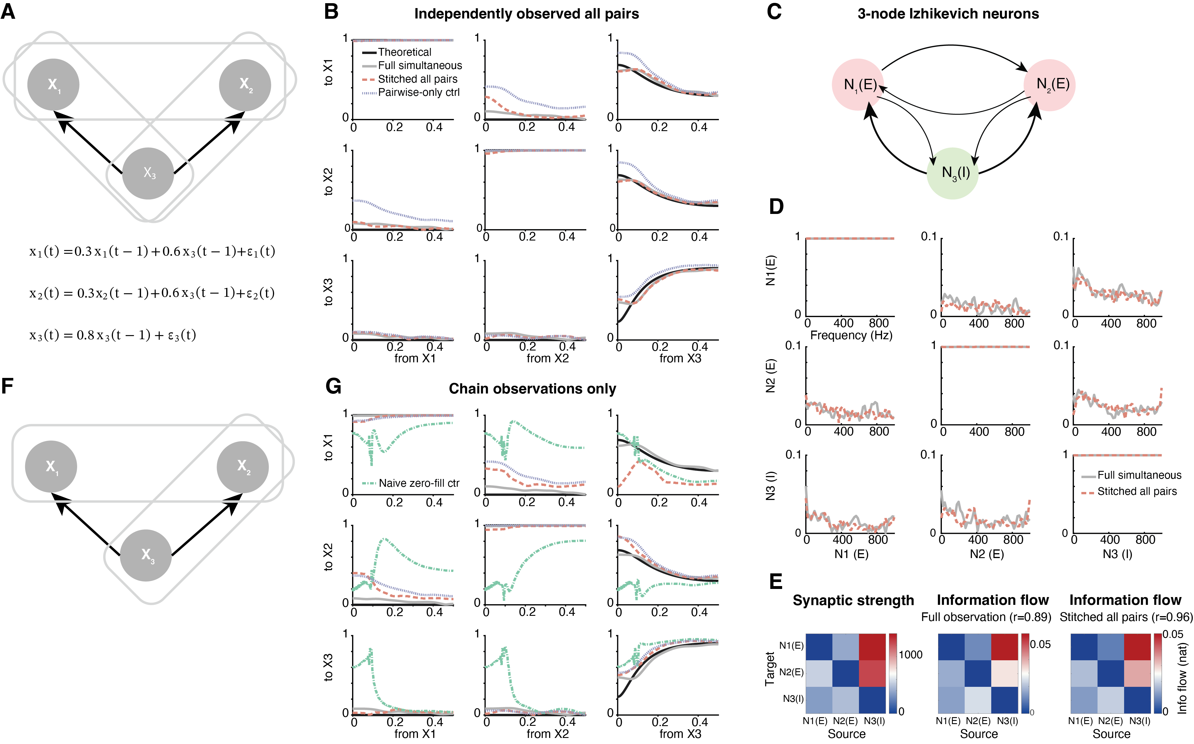
We first verify the method on a small system where the ground truth is known analytically. Time series are simulated from a stationary VAR(1) process (Fig 2A). We model exactly the situation in which drives both and but and have no direct interaction. All pairs are observed in independent blocks, satisfying Condition 1. We compare four estimates: the theoretical PDC obtained from the Fourier transform of the VAR(1) coefficients, the non-parametric PDC computed from a single fully simultaneous recording via (7), the SPIDER estimate obtained from the asynchronous blocks via Algorithm A.4, and a pairwise-only control that estimates local PDC without integrating information across blocks. The SPIDER estimate tracks the simultaneous estimate almost exactly across all pairs and frequencies, and both closely approximate the theoretical PDC (Fig 2B). The pairwise-only control deviates systematically, especially between and , where interaction does not exist in reality, confirming that aggregating the full spectral matrix across blocks is necessary to recover the correct directed structure. Together, this confirms that asynchronous block recordings, when each pair is jointly observed at least once, contain the same directional information as a single simultaneous recording.
The VAR framework underlying the theoretical guarantees assumes linear dynamics, yet many real systems of interest, including neural circuits, are inherently nonlinear. We therefore test whether the stitching pipeline generalizes to a biophysically realistic network of Izhikevich spiking neurons, which exhibit nonlinear spike generation. The network consists of two excitatory neurons and and one inhibitory neuron , connected with known directed synaptic weights (Fig 2C; see Appendix F for model details). Because spike trains are point processes, we apply the multi-taper point-process spectral estimator of (17) [36]. The SPIDER estimates closely track the full-simultaneous reference across all nine entries of the PDC matrix and across the frequencies (Fig 2D), demonstrating that the pipeline handles the spike-timing dynamics without degradation. Because the estimate is recovered at every frequency (Fig 2D), directed interactions can be localized to specific frequency bands; the integrated information-flow summaries used for the larger comparisons below collapse this axis for compactness. To assess biological validity, we compare the estimated directed information flow to a ground-truth effective influence matrix derived from the simulated network. The matrix is computed as synaptic coupling strength multiplied by presynaptic firing rate, providing a proxy for the expected rate of information transmission along each connection (Fig 2E). Both the full-simultaneous estimate (Pearson ) and the SPIDER estimate () recover the synaptic organization faithfully. Together, these results demonstrate that SPIDER generalizes beyond linear Gaussian processes to the nonlinear, point-process setting that characterizes real neural recordings.
3.2 Matrix completion enables recovery under incomplete pairwise observation
We next consider the case where Condition 1 fails. Using the same three-node VAR(1) system, we adopt a chain observation design in which only the pairs and are jointly observed, while is never co-observed (Fig 2F). Recall that the true structure has driving both and with no direct – interaction; because is observed with but not with , any local estimate restricted to the block will conflate the shared driver with a spurious direct connection. SPIDER estimates obtained via NNM recover the directed structure more accurately than the local pairwise control across all observed directions, and in particular substantially mitigate the spurious – interaction that contaminates local estimates (Fig 2G). The residual spurious component is not fully eliminated, consistent with the fact that the cross-spectrum must be inferred. By contrast, a naive baseline that fills missing entries of with zeros fails to reproduce even some of the observed entries (e.g., ), illustrating that ignoring missingness is not benign: errors in unobserved entries propagate to observed ones through the inversion and factorization steps.
3.3 High-dimensional performance and the role of completion
To assess performance in higher dimensions, we simulate -dimensional stationary VAR(1) processes with randomly generated full-rank coefficient matrices and threshold to achieve target sparsity levels of 5%, 50%, 75%, and 95% zeros. Innovations are i.i.d. Gaussian with covariance . Each simulation runs for time steps after discarding burn-in samples. Observation blocks are constructed as contiguous, partially overlapping subsets of the variables with a fixed overlap ratio of 50% between adjacent blocks; varying the block size ratio across {0.1, 0.2, 0.4, 0.6} yields the four missingness levels of 30%, 48%, 72%, and 86% shown in the Fig 3. All results are averaged over 10 independent replicates. For each configuration, we compute the MSE of the off-diagonal entries of the SPIDER estimate against two references: the theoretical PDC computed from the known VAR(1) coefficients (Fig 3A), and the non-parametric PDC from a single fully simultaneous recording, which serves as a finite-sample oracle upper bound (Fig 3B).
We compare seven conditions (Fig 3A-B): SPIDER estimates with NNM completion for all off-diagonal pairs, observed pairs, and never-observed pairs; a local baseline that estimates PDC only within each observation block, restricted to co-observed pairs and conditioned solely on observed variables; and the corresponding three subsets of the naive zero-fill baseline. The local baseline directly answers the question of what ignoring asynchrony would obtain: each block is restricted to pairs within and conditioned only on , not on the full . As discussed above, this is a fundamentally different estimand from the whole-network PDC, and per-block estimates are subject to confounding by unobserved variables.
SPIDER with NNM completion produces significantly lower MSE than the naive zero-fill baseline for both references (, paired t-test), and at low to moderate missingness (72%), it outperforms the local per-block baseline for observed pairs (, paired t-test; Fig 3A&B). At very high missingness, the advantage of the NNM stitching reduces, especially for unobserved pairs: when most entries are unobserved, the structural prior cannot compensate for the lack of information, and completion becomes unreliable. The transition from the regime in which completion meaningfully helps to the regime in which it does not is consistent with the coverage condition of Proposition 3: as falls below , the nuclear-norm program loses its consistency guarantees. The local per-block baseline becomes more advantageous if missingness is high: at 86% missingness, it outperforms SPIDER.

3.4 Effect of GLASSO regularization
We next isolate the contribution of the GLASSO regularization step by varying both the regularization strength and the sparsity of the underlying VAR coefficient matrix. When using the theoretical PDC as reference, the benefit of GLASSO regularization () depends jointly on missingness and coefficient-matrix sparsity (Fig 3C). When the underlying connectivity is sparse, GLASSO regularization reduces the error of the SPIDER estimate, with the largest gains at low missingness. As sparsity decreases, the benefit of regularization shrinks, and at very dense connectivity GLASSO can hurt accuracy. When compared against the simultaneous-recording reference, the regularization choice outperforms the unregularized estimator across all sparsity levels, indicating that even when the true coefficient matrix is dense, the penalty corrects for finite-sample variance introduced by the stitching and completion steps (Fig 3D). MSE increases monotonically with missingness under all conditions.
3.5 Application to calcium imaging
We applied the method to two-photon calcium imaging data from mouse visual cortex in the Allen Brain Observatory [22]. We analyzed a 600 s spontaneous-activity segment ( 18,000 samples at 30 Hz) during which 227 neurons were recorded simultaneously. To ensure reliable information-flow estimation, we restricted the analysis to neurons exhibiting sufficient activity (dF/F signal exceeding standard deviations for at least 200 time points), yielding 59 neurons. PDC here is computed on the dF/F signal rather than on deconvolved spike rates, so the recovered interactions reflect dynamics at the timescale resolved by the calcium indicator and should not be over-interpreted at faster timescales.
To assess estimation stability under finite samples, we examined how non-parametric PDC estimates depended on recording duration. Treating the full 600 s segment as a reference, we computed the mean squared error between PDC magnitudes estimated from shorter segments and the full-data estimate, excluding diagonal entries. Error decreased systematically with increasing data length, with a pronounced drop around 200 s (approximately one-third of the recording), beyond which improvements were gradual (Fig 4A). The Pearson correlation between integrated information-flow matrices (2) estimated from truncated and full data increased monotonically with sample size, indicating convergence. These results suggest that stable PDC estimation is achievable at the data lengths considered.
We then divided the recording into three sequential time blocks with 50% neuron overlap (overall missingness ) and applied SPIDER with NNM completion. The reconstructed information flow matrix recovered many of the strongest directed interactions observed under full simultaneous recording (Fig 4B,C). Observed entries showed strong agreement with the simultaneous-recording reference (). Imputed entries also exhibited a significant positive correlation with the reference (, ; Fig 4D), demonstrating partial recovery of unobserved interactions consistent with the simulation results above.
We examined the effect of GLASSO regularization on reconstruction accuracy. Moderate regularization significantly reduced error (, ), while overly strong regularization degraded performance through excessive sparsification (Fig 4E). Regularization reduced error for observed interactions but increased error for imputed ones, consistent with over-attenuation of weak inferred connections. Despite these effects on error magnitude, the overall information-flow pattern was largely preserved: Pearson correlations with the simultaneous-recording reference remained stable across (Fig 4F). The principal difference was between observed and imputed entries, with imputed entries showing systematically lower correlations () but remaining significantly above zero for all tested ().
Together, these results show that SPIDER robustly recovers directed information flow from partial and asynchronous neural recordings, with regularization primarily improving stability without altering the dominant directional structure.

3.6 Application to Neuropixels data
Neuropixels probes enable simultaneous recording of hundreds of single neurons in multiple brain areas, including deep subcortical structures. When aligned to a standard brain atlas, the shared area annotations across animals provide the anchor for stitching directed information flow across sessions, animals, and laboratories. We applied our method to the International Brain Laboratory (IBL) brain-wide map dataset [38, 37], comprising Neuropixels recordings collected across 12 laboratories under a standardized experimental pipeline targeting 279 brain areas in 139 adult mice. To avoid stimulus-locked responses, we restricted the analysis to passive and spontaneous activity epochs, which lasted approximately 600 seconds per session.
Recordings were subject to a multi-stage quality control pipeline. We retained only neurons classified as good isolated units by the automated spike-sorting quality metrics, restricted to sessions with at least two valid brain areas simultaneously recorded, and excluded fiber tract regions. At the neuron level, units with a mean firing rate below 0.2 Hz were discarded to ensure sufficient spike counts for stable spectral estimation. At the area level, we required at least 5 simultaneously recorded neurons per area, and further excluded areas whose spectral PC1 explained less than 10% of the total spectral variance, which we used as a data-driven threshold indicating insufficient shared population-level structure.
The area-level SPIDER procedure (stitching via matched brain areas) is detailed in Methods and illustrated in Fig 5A. Since no ground-truth directed connectivity exists for the full set of brain areas, we validated the approach in three complementary ways.
Validation 1: within-session split
Within the same session, the simultaneously recorded full set of areas provides an upper bound on estimation accuracy. To assess how closely stitching approximates this bound, we artificially partitioned each session into two halves, each covering a different but partially overlapping subset of brain areas, and then compared the SPIDER estimate against the PDC estimated from the full simultaneous observation (Fig 5B). In two sessions with 20 randomized brain area assignments each, the overall agreement between the SPIDER and fully-observed PDC was high (, mean SD; Fig 5C). Area pairs that were co-observed showed strong agreement () and pairs requiring imputation were weaker (). This result confirms that our area-level SPIDER approach is feasible.
Validation 2: local spectral consistency predicts stitching accuracy
Theorem 1 guarantees convergence of the SPIDER estimate provided that local spectral consistency holds across sessions. To test whether this condition is met empirically, and to derive a principled session-selection threshold, we identified 20 target sessions with a relatively large number of simultaneously recorded areas () and, for each, designated two source sessions sharing a partially overlapping subset of areas (Fig 5D). We used the area-level cross-spectral density (CSD) and PDC of the target session as reference, and measured (i) the Pearson correlation between the source and target CSDs and (ii) the correlation between the SPIDER information flow derived from the source sessions and the target PDC. Across all 20 sessions, higher source-target CSD similarity was associated with higher SPIDER information-flow accuracy (Spearman correlation , ; Fig 5E), indicating that local spectral consistency is a strong predictor of stitching accuracy. From this relationship, we determined the session-selection threshold as the CSD-correlation value at the zero-crossing of the lower 95% confidence band of the fitted regression line for the observed pairs (Fig 5E).
Validation 3: correspondence with anatomical connectivity
Applying the threshold determined in Validation 2, we identified the largest stitchable graph whose missingness remained below the limit (70%) identified in simulation (Fig 3), beyond which stitching accuracy becomes indistinguishable from that of null models. Maximizing area coverage while keeping missingness below this bound, the final dataset retained 43 sessions from 12 laboratories, encompassing 50 brain areas and 4,074 neurons (Fig 5F & G; see Appendix G for session and brain area information). The selected sessions spanned cortical, hippocampal, thalamic, and midbrain regions, providing broad coverage of the mouse brain’s major functional subsystems.
As an indirect validation, we compared the SPIDER directed information flow to structural connectivity from the Allen Mouse Brain Connectivity Atlas [40], which provides whole-brain anterograde axonal tracing data. For each pair of areas in the stitched graph, we quantified directed anatomical connectivity as the maximum anterograde projection density from the source area to the target area. Sweeping the binarization threshold of the Allen projection matrix and computing the ROC curve against the SPIDER estimate yielded AUC values approaching 0.9 at high thresholds, indicating that the most prominent anatomical projections were reflected in the estimated information flow (Fig 5H). The AUC for observed area pairs was consistently above chance, whereas unobserved pairs showed near-chance AUC. The anatomical correspondence is therefore carried by the directly co-observed pairs; directed edges between areas that were never co-recorded are recovered only through completion and should be read with corresponding caution.
Taken together, these three complementary validations establish that independently recorded Neuropixels datasets can be integrated across sessions, animals, and laboratories to recover directed information flow among brain areas that were never simultaneously recorded.

3.7 A theta-band feedforward hierarchy of spontaneous information flow
The validations above establish that SPIDER recovers directed information flow faithfully; we next asked whether the recovered brain-wide network carries interpretable organization that no single session could reveal. A directed network is feedforward, or hierarchical, to the extent that its edges can be arranged so that influence flows consistently from lower to higher levels, and recurrent to the extent that flow circulates in loops or is reciprocated. We quantified this with the trophic-incoherence framework of MacKay, Johnson and Sansom [46, 47], which assigns each area a continuous trophic level from the directed flow and measures the departure from a perfect feedforward hierarchy by an incoherence index (, perfectly feedforward; , no hierarchy; Fig 6A and Appendix A.5). Significance was assessed against a direction-randomized null that preserves every undirected interaction strength but scrambles its direction.
Integrated over all frequencies, the SPIDER network was essentially non-hierarchical (, indistinguishable from the direction-shuffled null, ): brain-wide spontaneous flow is, on the whole, recurrent. Resolving the estimate by frequency revealed a sharply localized exception. Trophic incoherence dropped to a single narrow minimum in the theta band (4–8 Hz; , , against the null, surviving Bonferroni correction across five bands); a continuous frequency sweep confirmed a single minimum localized to the theta range (Fig 6B). The theta ordering was robust—leave-one-area-out jackknifing left it essentially unchanged (Spearman )—and incoherence rose monotonically with frequency, so that by the gamma range the network was statistically indistinguishable from a directionless graph.
The theta hierarchy had a consistent anatomical polarity (Fig 6C): the hippocampal formation (subiculum, dentate gyrus, CA1) and ventral striatum (nucleus accumbens) occupied the source end, while midline and mediodorsal thalamus, periaqueductal gray, and medial prefrontal cortex (infralimbic area) formed the sinks. Decomposing the total directed flow into a feedforward gradient, a circulating (loop) component, and a reciprocal (mutual) component made the frequency dependence explicit (Fig 6D): reciprocal flow dominated in every band and grew from roughly one half in theta to in high gamma, whereas the feedforward share peaked in theta—about half of the total flow, with of the theta net flow directed up the hierarchy—and collapsed toward gamma.
Two points deserve emphasis. First, the finding is intrinsic to the data and required no anatomical prior: the hierarchy is read out from the directed spectra themselves. Second, it is a frequency-specific directional effect—feedforward in theta, recurrent in gamma—of exactly the kind that is invisible to time-domain or scalar connectivity measures and that emerges only because SPIDER recovers whole-network, frequency-resolved direction from data that were never recorded together. That theta is the band in which spontaneous brain-wide flow organizes into a hierarchy, with the hippocampal formation at its apex, is consistent with the established role of theta in coordinating hippocampal–cortical communication [48, 49]. We report this as a hypothesis-generating result: it rests on passive and spontaneous epochs and on directly co-observed area pairs, and it is an effective-connectivity statement rather than a claim about monosynaptic anatomy.

3.8 Application to human intracranial EEG
To test whether SPIDER transfers to human recordings, we applied it to the open multimodal iEEG dataset of Berezutskaya et al. [4] (OpenNeuro ds003688), comprising intracranial EEG from 51 patients implanted with subdural grids and stereo-EEG depth electrodes for presurgical monitoring. Here the stitching anchor is anatomical rather than experimental: each patient’s electrodes were normalized to MNI space and labeled with the automated anatomical labeling (AAL) atlas [5], so that shared atlas regions play the role that shared brain areas played for the Neuropixels data, and patients play the role of sessions. As in the rodent analysis, we restricted attention to resting, spontaneous recordings. After retaining good-quality SEEG/ECoG channels and re-referencing to nearest-neighbor bipolar derivations within each electrode shaft, the bipolar cross-spectra were estimated by continuous multitaper—in place of the point-process estimator used for spike trains—each region was reduced to a single canonical spectral mode by spectral PCA (exactly as areas are reduced in the Neuropixels analysis), and the resulting region-by-region cross-spectra were passed unchanged to the stitching, completion, and Wilson-factorization steps. Because electrode coverage in this cohort is strongly left-lateralized, we report the left hemisphere. The final stitched graph comprised 38 left-hemisphere cortical AAL regions pooled from 43 patients, none recorded together, of which () region pairs were directly co-observed in at least one patient; the remaining pairs were recovered by completion, a missingness () well within the regime in which stitching is reliable (Fig 3).
SPIDER returned a directed whole-cortex information-flow estimate across the 38 regions (Fig 7A), recovered entirely from patients that were never recorded together. Applying the same trophic-incoherence analysis used for the rodent network, the directed hierarchy was strongly concentrated in the theta band: trophic incoherence was low in theta (, a pronounced feedforward hierarchy) and rose to near the recurrent limit by gamma (, i.e. only marginally hierarchical; Fig 7B). Against a direction-shuffled null—preserving each pair’s undirected interaction strength but scrambling its direction—theta was overwhelmingly significant (, , Bonferroni-corrected). The higher bands also cleared this tight null ( from to ) but only weakly in absolute terms, and this residual high-band gradient may partly reflect the completion step; the dominant and interpretable effect is a theta-band feedforward hierarchy. The theta hierarchy had an interpretable polarity (Fig 7C): ventromedial and paralimbic cortex—olfactory cortex, temporal pole, insula, and medial and orbital prefrontal cortex—occupied the source end, while lateral prefrontal and temporal cortex and early visual areas (calcarine, lingual) formed the sinks. The hippocampal formation, the apex of the rodent theta hierarchy, is subcortical and excluded here, but the cortical source end is precisely the paralimbic system with which it is most tightly coupled. Thus the theta-band feedforward hierarchy that SPIDER uncovered in the rodent brain re-emerges in human resting cortex, recovered from single-patient recordings that were never acquired together—a replication across species and recording modality that no individual dataset could yield.

4 Discussion
We have introduced SPIDER, a non-parametric framework for recovering frequency-domain directed information flow from asynchronous and partially observed neural recordings. The central practical advance for neuroscience is that the method removes the two requirements that have confined directed effective-connectivity analysis to single, fully simultaneous recordings: it needs neither simultaneous observation of all regions nor a shared temporal reference. Because the estimate is frequency-resolved, it captures directed interactions at distinct timescales rather than reducing each connection to a single summary value. As a result, it can reveal band-specific patterns of influence, such as theta- versus gamma-range interactions, that are inaccessible to time-domain or scalar connectivity measures. Under the completeness condition, the stitched spectral estimator and the resulting non-parametric PDC are uniformly consistent for all variable pairs (Theorem 1). When completeness fails, consistent recovery remains possible if a structured matrix completion step succeeds (Theorem 2); we identify spikiness of the spectrum, sufficient pairwise coverage, and near-low-rank structure as one concrete set of conditions under which nuclear-norm minimization meets that requirement (Proposition 3). The simulation results confirm these theoretical predictions: NNM completion outperforms a naive zero-fill baseline at low to moderate missingness, GLASSO regularization reduces error when the underlying connectivity is sparse, and directed structure is recovered accurately for observed pairs and partially for imputed ones, degrading as pairwise coverage falls. The application to the Allen Brain Observatory data demonstrates that the method scales to real neural recordings of moderate dimension and recovers the dominant directional structure even with substantial missingness. Applied to the IBL brain-wide Neuropixels dataset, the area-level variant recovers directed information flow across 50 brain regions by stitching data from 43 sessions collected in 12 laboratories, none of which were recorded simultaneously. The strongest inferred interactions show substantial correspondence with anatomical projections from the Allen Institute for Brain Science, achieving ROC–AUC values approaching for observed region pairs. Applied to resting human intracranial EEG, the same pipeline reconstructed a directed whole-cortex network by pooling 43 patients with non-overlapping electrode coverage, and recovered the same theta-band feedforward hierarchy—significant against a direction-shuffled null—demonstrating the finding across species and recording modality. Across these applications the method operated at the tens-to-hundreds-channel scale of current recordings; the asymptotic regime in which the number of variables greatly exceeds the per-block sample size is characterized in simulation.
4.1 A frequency-specific hierarchy of spontaneous flow
Beyond validating the estimator, the IBL analysis yields a concrete neuroscientific result: integrated over frequency, the brain-wide directed network is recurrent, but in the theta band it reorganizes into a statistically significant feedforward hierarchy with the hippocampal formation at its source and thalamo-frontal and midbrain structures as sinks, while higher frequencies remain dominated by reciprocal flow (Fig 6). This band-specific directionality—feedforward in theta, recurrent in gamma—is precisely the kind of structure that scalar or time-domain connectivity measures cannot express, and it could only be read out by pooling sessions that were never recorded together. It is consistent with the role of theta in organizing hippocampal–cortical communication [48, 49], the hippocampal formation being both a principal generator of theta and, through the subiculum, its main output stage. The same theta-band hierarchy re-emerges in resting human intracranial EEG (Fig 7), recovered by pooling patients with non-overlapping coverage, with its cortical source in ventromedial and paralimbic cortex—indicating that the organization is not specific to the rodent or to spike-based recording.
A more tentative observation concerns the apex of the theta hierarchy, the periaqueductal gray (PAG), which received far more directed flow than it emitted. Within our data this sink position rests on limited evidence—the PAG was directly co-observed with only six other areas—and its measured theta input was dominated by the hippocampal formation (notably CA1 and dentate gyrus), consistent with the PAG being entrained as a recipient within the hippocampal theta-coordinated network rather than with any specific hippocampo-PAG projection. This position is at least compatible with the PAG’s established role as a convergence hub and obligatory final premotor gate for diverse innate behaviors—from defensive responses [50, 51] to vocalization, where a dedicated PAG population is necessary and sufficient to gate ultrasonic calls in mice [52, 53]—a role under which a net-recipient signature is unsurprising. We deliberately avoid a stronger reading: the descending forebrain pathways classically associated with the PAG, from medial prefrontal, cingulate and amygdalar regions, were not co-observed with it here and so could not be assessed, and the PAG’s own brainstem premotor targets lie outside the recorded set; the node-level interpretation therefore awaits recordings that co-sample the PAG with its forebrain afferents. We frame the hierarchy as a whole as hypothesis-generating: it rests on passive, spontaneous epochs and on directly co-observed area pairs, it is an effective-connectivity rather than an anatomical claim, and it illustrates that frequency-resolved effective connectivity at brain-wide scale can surface testable hypotheses about the directional architecture of spontaneous activity.
4.2 Pooling across sessions and animals
The independence of stitching from temporal alignment is what makes the framework applicable to data pooled across sessions or animals: blocks need not share a clock, and only the marginal spectral statistics within each block enter the estimator. The key remaining requirement when pooling across heterogeneous sources is that blocks be exchangeable samples from approximately the same generative process. In practice this is the standard assumption underlying any pooled analysis of population recordings; it can be checked by comparing within-block spectra across blocks before stitching, and violations can be detected as anomalous local PSD estimates that disagree on overlapping channels.
4.3 Non-stationarity
Although the theory assumes wide-sense stationarity, the method extends straightforwardly to mildly non-stationary settings via standard segmentation or windowed spectral estimation, under the assumption that signal statistics vary slowly relative to the window length. Note that this requires a time axis only within each block, so that its windows are mutually comparable; it does not reintroduce the shared temporal reference across blocks that the method otherwise avoids. This is the same approach taken by virtually all spectral analyses of neural data and does not require modification of the stitching, completion, or regularization steps. When a recording spans changes in brain state, however, within-window non-stationarity biases the spectral estimate; restricting to passive or spontaneous epochs limits but does not eliminate this, and comparing estimates across sub-windows provides a simple diagnostic.
4.4 Limitations
The theoretical guarantees presented here are sufficient conditions, and the constants appearing in the scaling requirements are typically unknown and may depend on the data. Practitioners should treat these conditions as order-of-magnitude guides rather than sharp thresholds and, where possible, use diagnostics—such as the condition number of the stitched matrix, cross-validation of the GLASSO penalty, and the completion residual on held-out co-observed entries—to assess whether the method is operating in a reliable regime. With this caveat, four failure modes are worth flagging explicitly.
Long-memory processes. The local PSD consistency on which the entire pipeline rests requires exponential decay of the dependence-adjusted norm of each component series [41]. Processes with polynomially decaying correlations, such as long-memory or fractionally integrated processes, fall outside this condition, and spectral estimation may be unreliable in those regimes. The downstream PDC consistency results no longer apply.
Insufficient pairwise coverage. NNM completion requires the coverage condition of Proposition 3. If the recording design yields fewer co-observed pairs, equivalently, if the per-pair observation probability satisfies , completion is not guaranteed to recover the missing entries, and PDC estimates for unobserved pairs will be unreliable. The simulation results show that performance on unobserved pairs degrades sharply as missingness exceeds approximately , consistent with this prediction.
High effective rank. If does not admit a good low-rank approximation, for example, when activity is driven by many independent sources of comparable strength rather than a small number of dominant ones, the approximation error in the completion bound does not vanish and the near-low-rank assumption fails. In this regime, completion provides little benefit over zero-filling.
High correlation and ill-conditioning. When observed signals are highly correlated, the spectral matrix is near-singular and any method that requires its inversion or factorization, including ours, becomes numerically unstable. This is a fundamental difficulty rather than a limitation specific to stitching. Strong external sources driving the dynamics, or redundant channels recording overlapping signals, are typical causes. Pre-processing such data by clustering channels or extracting latent components prior to causal analysis is a sensible, practical mitigation.
4.5 Future directions
Several extensions are natural. First, alternative completion algorithms with different structural priors, such as nonconvex factorizations, weighted nuclear-norm variants, and explicit factor-model approaches, could be substituted for the nuclear-norm program in Step 2 of Algorithm A.4, with the conditional structure of Theorem 2 ensuring that any such substitution that achieves uniform completion consistency yields PDC consistency. Second, the framework could be combined with hypothesis-testing procedures to produce calibrated confidence statements on individual directed edges, building on recent work in high-dimensional spectral inference. Third, because the pipeline decomposes into independent computations at each frequency, it is readily amenable to GPU acceleration, which could substantially expand the dimensionality of networks that can be analyzed in practice.
5 Conclusion
By eliminating the need for both simultaneous observation of all variables and a shared temporal reference, SPIDER enables systematic whole-brain analysis of multi-session and multi-animal datasets that could not previously be combined for directed-flow inference. It turns the fragmented, asynchronous recordings that brain-wide initiatives already produce into a single, frequency-resolved map of directed effective connectivity, and does so non-parametrically for continuous signals, spike trains, and their mixtures alike. We expect this to broaden the range of experimental designs from which whole-brain information flow can be studied.
Funding
D.Y.T. was supported by CNPq grants 421955/2023-6 and 445096/2024-1, FAPESP grant 2013/07699-0, and Serrapilheira grant R-2401-47364. Y.S.Z. thanks CAPES-PRINT UFRN 88887.979326/2024-00, for supporting a one-month visit to the Brain Institute, UFRN, and National Natural Science Foundation of China (grant 2025ZD0215700).
Data and code availability
The two-photon calcium-imaging data are publicly available through the Allen Brain Observatory [22] at https://observatory.brain-map.org/visualcoding/search/cell_list?experiment_container_id=511510989&sort_field=p_sg&sort_dir=asc. The Neuropixels electrophysiology data through the International Brain Laboratory brain-wide map [37]. The human intracranial EEG data are publicly available on OpenNeuro (ds003688) [4] at https://openneuro.org/datasets/ds003688. Code implementing the SPIDER pipeline, together with the processed spectral matrices and area annotations required to reproduce the figures, can be found at https://github.com/yisiszhang/stitched_pdc.git.
Declaration of generative AI use
During the preparation of this work, the authors used ChatGPT and Claude to help with coding and text editing. The authors reviewed and edited the output as needed and take full responsibility for the content of the published article.
References
- [1] Friston KJ, Harrison L, Penny W. Dynamic causal modelling. NeuroImage. 2003;19(4):1273–1302.
- [2] Seth AK, Barrett AB, Barnett L. Granger causality analysis in neuroscience and neuroimaging. Journal of Neuroscience. 2015;35(8):3293–3297.
- [3] Bastos AM, Schoffelen JM. A tutorial review of functional connectivity analysis methods and their interpretational pitfalls. Frontiers in Systems Neuroscience. 2016;9:175.
- [4] Berezutskaya J, Vansteensel MJ, Aarnoutse EJ, Freudenburg ZV, Piantoni G, Branco MP, et al. Open multimodal iEEG-fMRI dataset from naturalistic stimulation with a short audiovisual film. Scientific Data. 2022;9:91.
- [5] Tzourio-Mazoyer N, Landeau B, Papathanassiou D, Crivello F, Etard O, Delcroix N, et al. Automated anatomical labeling of activations in SPM using a macroscopic anatomical parcellation of the MNI MRI single-subject brain. NeuroImage. 2002;15(1):273–289.
- [6] Walden AT. A unified view of multitaper multivariate spectral estimation. Biometrika. 2000;87(4):767–788.
- [7] Wilson GT. A convergence theorem for spectral factorization. Journal of Multivariate Analysis. 1978;8(2):222–232.
- [8] Friedman J, Hastie T, Tibshirani R. Sparse inverse covariance estimation with the graphical lasso. Biostatistics. 2008;9(3):432–441.
- [9] Gelfand IM, Iaglom A. Calculation of the amount of information about a random function contained in another such function. American Mathematical Society Translation Series. 1959;2:3–52.
- [10] Amblard PO. A nonparametric efficient evaluation of partial directed coherence. Biological Cybernetics. 2015;109(2):203–214.
- [11] Jarvis M, Mitra PP. Sampling properties of the spectrum and coherency of sequences of action potentials. Neural computation. 2001;13(4):717–749.
- [12] Takahashi DY, Baccalá LA, Sameshima K. Information theoretic interpretation of frequency domain connectivity measures. Biological cybernetics. 2010;103:463–469.
- [13] Baccalá LA, Sameshima K. Partial directed coherence: a new concept in neural structure determination. Biological cybernetics. 2001;84(6):463–474.
- [14] Chang A, Zheng L, Dasarathy G, Allen GI. Nonparanormal graph quilting with applications to calcium imaging. Stat. 2023;12(1):e623.
- [15] Vinci G, Dasarathy G, Allen GI. Graph quilting: graphical model selection from partially observed covariances. arXiv preprint arXiv:191205573. 2019;.
- [16] Liu G, Li P. Low-rank matrix completion in the presence of high coherence. IEEE Transactions on Signal Processing. 2016;64(21):5623–5633.
- [17] Bishop WE, Yu BM. Deterministic symmetric positive semidefinite matrix completion. Advances in Neural Information Processing Systems. 2014;27.
- [18] Fan Y, Han F, Park H. Estimation and Inference on Granger Causality in a Latent High-Dimensional Gaussian Vector Autoregressive Model. Working Paper. 2020;.
- [19] Stringer C, Pachitariu M, Steinmetz N, Reddy CB, Carandini M, Harris KD. Spontaneous behaviors drive multidimensional, brainwide activity. Science. 2019;364(6437):eaav7893.
- [20] Baccala LA, Sameshima K, Takahashi DY. Generalized partial directed coherence. In: 2007 15th International conference on digital signal processing. Ieee; 2007. p. 163–166.
- [21] Thomson DJ. Spectrum estimation and harmonic analysis. Proceedings of the IEEE. 2005;70(9):1055–1096.
- [22] de Vries SE, Lecoq JA, Buice MA, Groblewski PA, Ocker GK, Oliver M, et al. A large-scale standardized physiological survey reveals functional organization of the mouse visual cortex. Nature neuroscience. 2020;23(1):138–151.
- [23] Granger CW. Investigating causal relations by econometric models and cross-spectral methods. Econometrica: journal of the Econometric Society. 1969; p. 424–438.
- [24] Ljung L. System identification. In: Signal analysis and prediction. Springer; 1998. p. 163–173.
- [25] Schölkopf B, Locatello F, Bauer S, Ke NR, Kalchbrenner N, Goyal A, et al. Toward causal representation learning. Proceedings of the IEEE. 2021;109(5):612–634.
- [26] Pillow JW, Shlens J, Paninski L, Sher A, Litke AM, Chichilnisky E, et al. Spatio-temporal correlations and visual signalling in a complete neuronal population. Nature. 2008;454(7207):995–999.
- [27] Das A, Fiete IR. Systematic errors in connectivity inferred from activity in strongly recurrent networks. Nature Neuroscience. 2020;23(10):1286–1296.
- [28] Soudry D, Keshri S, Stinson P, Oh Mh, Iyengar G, Paninski L. Efficient” shotgun” inference of neural connectivity from highly sub-sampled activity data. PLoS computational biology. 2015;11(10):e1004464.
- [29] Hsiao C. Autoregressive modeling and causal ordering of economic variables. Journal of Economic Dynamics and Control. 1982;4:243–259.
- [30] Eichler M. Causal inference in time series analysis. Causality: Statistical perspectives and applications. 2012; p. 327–354.
- [31] Turaga S, Buesing L, Packer AM, Dalgleish H, Pettit N, Hausser M, et al. Inferring neural population dynamics from multiple partial recordings of the same neural circuit. Advances in Neural Information Processing Systems. 2013;26.
- [32] Kang J, Park HJ. Integration of partially observed multimodal and multiscale neural signals for estimating a neural circuit using dynamic causal modeling. PLOS Computational Biology. 2024;20(12):e1012655.
- [33] Qiao S, Sedillo JI, Brown KA, Ferrentino B, Pesaran B. A causal network analysis of neuromodulation in the mood processing network. Neuron. 2020;107(5):972–985.
- [34] Calhoun AJ, Pillow JW, Murthy M. Unsupervised identification of the internal states that shape natural behavior. Nature neuroscience. 2019;22(12):2040–2049.
- [35] Zhang YS, Takahashi DY, El Hady A, Liao DA, Ghazanfar AA. Active neural coordination of motor behaviors with internal states. Proceedings of the National Academy of Sciences. 2022;119(39):e2201194119.
- [36] Mitra PP, Pesaran B. Analysis of dynamic brain imaging data. Biophysical journal. 1999;76(2):691–708.
- [37] Angelaki D, Benson B, Benson J, Birman D, Bonacchi N, Bougrova K, et al. A brain-wide map of neural activity during complex behaviour. Nature. 2025;645(8079):177–191.
- [38] Laboratory IB, Banga K, Benson J, Bhagat J, Biderman D, Birman D, et al. Reproducibility of in vivo electrophysiological measurements in mice. Elife. 2025;13:RP100840.
- [39] Functional connectomics spanning multiple areas of mouse visual cortex. Nature. 2025;640(8058):435–447.
- [40] Oh SW, Harris JA, Ng L, Winslow B, Cain N, Mihalas S, et al. A mesoscale connectome of the mouse brain. Nature. 2014;508(7495):207–214.
- [41] Zhang C, Zhang D. Spectral inference for high dimensional time series. IEEE Transactions on Information Theory. 2025;71(4):2909–2929.
- [42] Negahban S, Wainwright MJ. Restricted strong convexity and weighted matrix completion: Optimal bounds with noise. The Journal of Machine Learning Research. 2012;13:1665–1697.
- [43] Cunningham JP, Yu BM. Dimensionality reduction for large-scale neural recordings. Nature neuroscience. 2014;17(11):1500–1509.
- [44] Brémaud P, Massoulié L. Power spectra of general shot noises and Hawkes point processes with a random excitation. Advances in Applied Probability. 2002;34(1):205–222.
- [45] Izhikevich EM. Simple model of spiking neurons. IEEE Transactions on Neural Networks. 2003;14(6):1569–1572.
- [46] MacKay RS, Johnson S, Sansom B. How directed is a directed network? Royal Society Open Science. 2020;7(9):201138.
- [47] Johnson S, Domínguez-García V, Donetti L, Muñoz MA. Trophic coherence determines food-web stability. Proceedings of the National Academy of Sciences. 2014;111(50):17923–17928.
- [48] Buzsáki G. Theta oscillations in the hippocampus. Neuron. 2002;33(3):325–340.
- [49] Colgin LL. Mechanisms and functions of theta rhythms. Annual Review of Neuroscience. 2013;36:295–312.
- [50] Bandler R, Shipley MT. Columnar organization in the midbrain periaqueductal gray: modules for emotional expression? Trends in Neurosciences. 1994;17(9):379–389.
- [51] Tovote P, Esposito MS, Botta P, Chaudun F, Fadok JP, Markovic M, et al. Midbrain circuits for defensive behaviour. Nature. 2016;534(7606):206–212.
- [52] Jürgens U. The neural control of vocalization in mammals: a review. Journal of Voice. 2009;23(1):1–10.
- [53] Tschida K, Michael V, Takatoh J, Han BX, Zhao S, Sakurai K, et al. A specialized neural circuit gates social vocalizations in the mouse. Neuron. 2019;103(3):459–472.
- [54] Buzsáki G. Rhythms of the Brain. Oxford University Press; 2006.
Appendix A Mathematical details of the SPIDER pipeline
This appendix collects the equations underlying the narrative in Materials and Methods. Appendix B and the following sections give the formal process classes, theorems, and proofs.
A.1 Partial directed coherence and its non-parametric form
Consider the -dimensional time series with and . The process admits a VAR representation of order if
| (4) |
where the are matrices and is an innovation process with for and . The autoregressive transfer function is for . The informational PDC from series to series (Eq. (1) of the main text) is , and the integrated information flow is given by Eq. (2).
For the non-parametric formulation we assume a PSD matrix that is bounded uniformly from below and above: for some constant and almost every ,
| (5) |
where means is positive semi-definite. Together with pure non-determinism this yields a canonical spectral factorization of the inverse spectrum: for almost all ,
| (6) |
equivalently with minimum-phase (the form produced by Wilson’s algorithm [7]). The PDC of (1) can then be written using only the inverse PSD and its factorization,
| (7) |
making explicit that PDC requires no finite-order autoregressive model.
A.2 Regularization, matrix completion, and consistency ingredients
Local consistency and high-dimensional scaling
The per-block estimators are required to be locally consistent.
Assumption 1 (Local spectral consistency).
For all and ,
| (8) |
where is the length of block .
This holds under standard mixing and moment conditions [6]; in high dimensions, the smoothed periodogram is consistent across all entries and frequencies with dimension allowed to grow nearly exponentially with sample size,
| (9) |
provided each component process has an exponentially decaying dependence-adjusted norm [41], with recommended bandwidth .
Complex Hermitian GLASSO
Because the stitched estimator need not be positive definite, we map the complex Hermitian matrix to its equivalent real symmetric form
| (10) |
and solve the real-symmetric GLASSO
| (11) |
with and . The regularized estimator is obtained by recombining the appropriate blocks of and inverting,
| (12) |
which is Hermitian positive definite with a stable inverse.
Near-low-rank prior and matrix completion
The completion step assumes that population activity is driven by latent sources through a linear mixing model
| (13) |
with independent low-power sensor noise , so that
| (14) |
which is full rank but approximately low rank. In the incomplete case the stitched matrix is only partially specified.
Definition 3 (Stitched PSD under incomplete observation).
Let satisfy but not necessarily Condition 1, let be the set of observed pairs, and let . The stitched PSD is
Missing entries are recovered by nuclear-norm minimization over Hermitian positive definite matrices (Algorithm A.4, Step 2). Modeling the observation pattern as random, with each pair observed independently with probability , the coverage condition of Proposition 3 becomes
| (15) |
which is mild whenever .
A.3 Area-level cross-spectra via multitaper estimation and spectral PCA
Let neuron in area , session , fire at times . Compute discrete prolate spheroidal sequences (DPSS) of length with time-bandwidth product , with taper Fourier transforms
| (16) |
The mean-rate-corrected tapered transform of neuron under taper is
| (17) |
where is the mean firing rate, and the neuron-level cross-spectral matrix has entries
| (18) |
Definition 4 (Area-level canonical cross-spectrum).
For areas , the area-level canonical cross-spectrum is the bilinear projection of the neuron-level PSD matrix onto the leading spectral eigenvectors:
| (19) |
where (spectral PC1) is the leading eigenvector of the within-area spectral decomposition
| (20) |
The phase ambiguity in is fixed so that the element of maximum absolute magnitude is real and positive,
| (21) |
An area is retained only if its frequency-averaged PC1 explained variance exceeds a threshold,
| (22) |
with here. Finally, to make local estimates commensurable across sessions, the area-level cross-spectra are normalized to coherence,
| (23) |
before assembly via (3) and factorization.
A.4 Algorithm
Algorithm 1. Stitched non-parametric partial directed coherence (SPIDER). When Condition 1 holds, skip Step 2.
A.5 Hierarchy of directed flow: trophic incoherence and flow decomposition
To characterize the directed network recovered in a given frequency band we use the integrated information-flow matrix of (2), writing for the flow from area to area and restricting to directly co-observed pairs. Following MacKay, Johnson and Sansom [46, 47], each area is assigned a trophic level as the solution of
with centered to fix the additive constant, where and are the weighted in- and out-strengths. The trophic incoherence
measures the flow-weighted dispersion of edges around a perfect one-level feedforward step: exactly when every edge ascends one level (a perfect hierarchy), and as directions become unstructured. Significance is assessed against a null ensemble that, for each unordered pair, swaps the two directed weights with probability one half, preserving all undirected strengths while destroying directional organization; we report the -score and empirical -value of the observed relative to this ensemble.
To separate kinds of feedback we decompose the directed flow into three nonnegative shares of the total throughput . The reciprocal (mutual) share is . The remaining net flow is split by a discrete Helmholtz–Hodge decomposition into a gradient (feedforward) part, the flow-weighted least-squares fit of by the level difference , and a divergence-free circulating (loop) part; the fraction of net-flow energy in the circulating part is the cyclicity, and its complement the feedforward gradient share. These three shares are reported per band in Fig 6D.
Appendix B Formal characterization of admissible processes
This section makes precise the class of processes to which the non-parametric pipeline applies and states the condition under which the canonical spectral factorization used throughout the main text exists. The spectra below are written with the normalization , where is the (matrix) covariance sequence; any overall positive scalar in this normalization cancels in the PDC of (7) and (1), so the choice is immaterial for the estimand.
B.1 Canonical spectral factorization
Definition 5 (Admissible spectrum).
A matrix-valued function is an admissible spectrum if (i) for almost every ; (ii) is integrable; and (iii) there is a constant with for almost every , where means is positive semi-definite.
Condition (iii) is exactly the boundedness assumption (5) of the main text; it implies in particular that is Hermitian positive definite almost everywhere and that is bounded, hence integrable.
Proposition 1 (Existence and uniqueness of the canonical factorization).
Let be an admissible spectrum. Then there exist a matrix-valued function and a constant Hermitian positive definite matrix such that
| (24) |
where is the boundary value of a function analytic and non-singular on the open unit disc with (the minimum-phase or canonical factor). The pair is unique. Equivalently, with , which is (6).
This is the multivariate Wiener–Hopf–Masani factorization theorem; the relevant sufficient condition is the Szegő requirement , which holds automatically under Definition 5(iii). Wilson’s algorithm [7] computes numerically and is the procedure used in Algorithm A.4. The non-parametric PDC of (7) is a continuous functional of and is therefore well-defined for every admissible spectrum, independently of any finite-order parametric representation.
B.2 Linear processes: VAR, VMA, and VARMA
Definition 6 (Vector linear processes).
Let be a -dimensional white-noise innovation sequence with , , and for . A zero-mean wide-sense stationary process is:
-
•
a process if with and ;
-
•
a process if with ;
-
•
a process if .
Writing and , each of these processes has spectrum
| (25) |
with for the VAR case and for the VMA case.
Condition 2 (Stability and minimum phase).
and for all , where is extended into the closed unit disc.
Under Condition 2 together with absolute summability, the spectrum (25) is an admissible spectrum in the sense of Definition 5, and its canonical factor coincides with . The infinite-order VAR representation is the natural data-generating model for the high-dimensional consistency result invoked in the main text (Eq (9)), and the exponential decay of assumed there is a special case of absolute summability.
B.3 Point processes and the Bartlett spectrum
Let be a -variate simple, stationary point process on , where counts events of type . Write for the (constant) mean intensity and let
| (26) |
denote the reduced second-order covariance density, where the Dirac term removes the atom that each process contributes to its own covariance at .
Definition 7 (Bartlett spectrum).
The Bartlett spectrum of is the Hermitian matrix measure with density
| (27) |
Definition 8 (Linear multivariate Hawkes process).
is a linear multivariate Hawkes process with baseline and excitation kernels if its conditional intensity is
| (28) |
where is the history up to time . The process is stable (stationary with finite intensity) if the spectral radius of is strictly less than one, in which case the stationary rates are .
Proposition 2 (Bartlett spectrum of the Hawkes process).
For a stable linear multivariate Hawkes process, with ,
| (29) |
which is of the canonical form (24) with and .
Equation (29) is the Bartlett power spectral measure of the Hawkes process [44]. Stability guarantees that is non-singular for all and analytic with analytic inverse on the unit disc, so is admissible and its canonical factor is . Consequently and the PDC of a Hawkes process is the normalization of defined in (7).
B.4 Mixed point-process and continuous-valued processes
Let consist of a -dimensional continuous-valued wide-sense stationary process and a -variate point process , jointly second-order stationary, with . The joint second-order structure is described by the block spectral matrix
| (30) |
where is the ordinary spectral density of , is the Bartlett spectrum (27) of , and the cross-blocks are the Fourier transforms of the cross-covariance densities between the continuous and event channels [11]. A natural generative model couples the two through a point process whose stochastic intensity has an autoregressive form driven by both past events and the continuous signal. Whenever the resulting joint spectrum is admissible in the sense of Definition 5, the canonical factorization of Proposition 1 applies to the full block matrix and the PDC of (7) is well-defined across all continuous and event channels. Estimation requires only a consistent estimate of each block: the continuous and Bartlett blocks and their cross-spectra are all obtained from the multitaper estimator, with the point channels entered as binary event sequences whose tapering implicitly smooths the underlying intensity.
Appendix C Consistency under complete stitching (Theorem 1)
Theorem 1 (Consistency of SPIDER under complete stitching).
Let be a -dimensional wide-sense stationary, purely non-deterministic process whose spectral density is bounded uniformly from above and below by positive constants. Assume Condition 1 (completeness) and Assumption 1 (local spectral consistency). Let be the stitched estimator of Definition 1, its GLASSO-regularized version (Algorithm A.4) with regularization parameter as , and the SPIDER estimator (Definition 2). Then for all ,
Remark (Verifiable scaling for high-dimensional regimes). Assumption 1 is the abstract requirement of Theorem 1, but for practitioners it is useful to note one concrete sufficient condition. Under exponential decay of the dependence-adjusted norm of each component series, the result of [41] guarantees uniform local spectral consistency provided (9) holds. The recommended bandwidth is , which optimally balances the polynomial dependence on and . In particular, may grow nearly exponentially in the per-block sample size, so Theorem 1 applies in genuinely high-dimensional regimes where would defeat classical spectral theory.
Proof.
Under Condition 1, every pair is contained in at least one observation block . By Assumption 1, for each block the local spectral estimator converges uniformly in probability to the corresponding submatrix . Since each entry of the stitched estimator is obtained by averaging a finite number of uniformly consistent estimators, it follows that
Because is uniformly bounded from above and below by positive constants, it is uniformly positive definite. Uniform convergence of implies that is also uniformly positive definite with probability tending to one. The GLASSO operator with regularization parameter defines a continuous family of mappings on the space of uniformly positive definite Hermitian matrices, and the limiting mapping at reduces to the identity. Hence
Uniform positive definiteness of implies the existence of a canonical minimum-phase spectral factorization , with invertible and continuous in and . By continuity of the spectral factorization mapping, uniformly implies that the corresponding estimated factors satisfy
The non-parametric partial directed coherence is a continuous functional of the inverse spectral factor and of , with normalization terms bounded away from zero by uniform positive definiteness. Continuity of matrix inversion and of the PDC mapping therefore yields
∎
Appendix D Conditional consistency under incomplete observation (Theorem 2)
Theorem 2 (Conditional consistency of SPIDER under incomplete observation).
Let be a -dimensional wide-sense stationary, purely non-deterministic process with spectral density bounded uniformly from below and above by positive constants. Let be observation blocks not necessarily satisfying Condition 1, and let denote the set of observed index pairs. Assume Assumption 1 (local spectral consistency). Let be the partially specified stitched estimator of Definition 3 and let be a completed estimator obtained from via a structured matrix completion procedure satisfying
| (31) |
Then the SPIDER estimator obtained via frequency-wise GLASSO regularization with satisfies, for all ,
Proof.
By assumption, the completed spectral estimator satisfies
Since the true spectral density is uniformly bounded from below and above by positive constants, it is uniformly positive definite. Matrix inversion is continuous on this set, yielding
Let denote the GLASSO estimator applied frequency-wise to with regularization parameter . Since the penalized likelihood objective is strictly convex and smooth on the space of uniformly positive definite matrices, the GLASSO mapping is continuous and reduces to the unregularized inverse as . Consequently,
Because is purely non-deterministic, admits a unique canonical (minimum-phase) spectral factorization with invertible and continuous in . Canonical spectral factorization is continuous with respect to uniform perturbations of the spectral density on compact frequency sets, so the factor obtained from satisfies
The non-parametric partial directed coherence is a continuous functional of the inverse spectral factor , involving only matrix entries, absolute values, and normalization by a denominator bounded away from zero. By the continuous mapping theorem,
∎
Appendix E Sufficient conditions for completion consistency (Proposition 3)
Proposition 3 (Sufficient conditions for completion consistency via nuclear-norm minimization).
The result follows from the matrix completion bounds of Negahban and Wainwright [42], applied frequency-wise. Their main theorem establishes that, under the spikiness condition and the coverage condition , the nuclear-norm penalized least-squares estimator recovers a near-low-rank matrix from noisy partial observations, with mean-squared Frobenius error decomposing into a stochastic term that vanishes as the noise variance shrinks and an approximation term that vanishes as the effective rank captures the matrix energy. In our setting, the noise on each observed entry is the local PSD estimation error , whose variance vanishes as under Assumption 1. The approximation term vanishes under the near-low-rank decomposition (14). To obtain uniform consistency across the frequency grid of size , a union bound contributes the additional factor that appears in coverage condition (ii). Translating to a per-pair observation probability gives (15). The conclusion of Theorem 2 then follows directly from the verified hypothesis (31).
Appendix F Izhikevich spiking neural network: model parameters and simulation details
F.1 Network architecture
The biophysically realistic validation network consists of neurons: two excitatory regular-spiking units and , and one inhibitory fast-spiking unit . All-to-all directed synaptic connectivity is encoded in the weight matrix (columns: pre-synaptic; rows: post-synaptic)
| (32) |
where positive entries denote excitatory synapses and negative entries denote inhibitory synapses. Diagonal entries are zero (no self-connections).
F.2 Single-neuron dynamics
Each neuron follows the Izhikevich two-variable model [45]:
| (33) | ||||
| (34) |
with the reset rule: if , then and . Here is the membrane potential (mV) and is a recovery variable. The neuron-specific parameters are given in Table 1.
| Neuron | (mV) | |||
|---|---|---|---|---|
| 0.02 | 0.200 | 1.0 | ||
| 0.02 | 0.200 | 1.0 | ||
| 0.06 | 0.225 | 1.0 |
The parameters for and correspond to the regular-spiking excitatory cell type; the elevated time-scale parameter and recovery sensitivity for correspond to a fast-spiking inhibitory interneuron [45].
F.3 External input
Each neuron receives independent stochastic input
| (35) |
where (mean drive), (noise amplitude), and is independent standard Gaussian white noise sampled at each millisecond time step. The mean drive is chosen to maintain spontaneous firing in all three neurons; the noise amplitude ensures irregular, non-periodic spiking consistent with in-vivo-like activity.
F.4 Simulation
The network was simulated for (200 s) using the standard Euler integration scheme with a 1 ms time step. Spike times were recorded whenever . Synaptic input from neuron to neuron was delivered as an instantaneous additive current at the time of each pre-synaptic spike, with no synaptic delay.
Appendix G IBL Neuropixels sessions and brain areas retained for SPIDER analysis
G.1 Overview
A total of 43 recording sessions from the International Brain Laboratory (IBL) brain-wide map dataset were retained after quality control and session-selection procedures described in the Methods. Sessions span 12 contributing laboratories and 39 individual adult mice (four mice each contributed two sessions). Each session is identified by the format lab__subject__date__session-number. Together the 43 sessions cover 50 distinct brain areas after Allen CCF hierarchical remapping.
G.2 Retained sessions
| # | Laboratory | Subject | Date | Areas recorded |
|---|---|---|---|---|
| 1 | angelakilab | NYU-11 | 2020-02-21 | 9 |
| 2 | angelakilab | NYU-37 | 2021-01-25 | 6 |
| 3 | angelakilab | NYU-45 | 2021-07-19 | 6 |
| 4 | churchlandlab | CSHL049 | 2020-01-09 | 4 |
| 5 | churchlandlab | CSHL051 | 2020-02-05 | 5 |
| 6 | churchlandlab | CSHL055 | 2020-02-17 | 6 |
| 7 | churchlandlab | CSHL058 | 2020-07-07 | 4 |
| 8 | churchlandlab | CSHL058 | 2020-07-08 | 5 |
| 9 | churchlandlab_ucla | MFD_05 | 2023-08-16 | 4 |
| 10 | churchlandlab_ucla | MFD_07 | 2023-08-31 | 4 |
| 11 | churchlandlab_ucla | UCLA033 | 2022-02-15 | 9 |
| 12 | churchlandlab_ucla | UCLA036 | 2022-03-09 | 7 |
| 13 | churchlandlab_ucla | UCLA037 | 2022-02-02 | 7 |
| 14 | cortexlab | KS044 | 2020-12-09 | 9 |
| 15 | cortexlab | KS046 | 2020-12-04 | 7 |
| 16 | cortexlab | KS051 | 2021-05-11 | 5 |
| 17 | cortexlab | KS096 | 2022-06-17 | 4 |
| 18 | danlab | DY_008 | 2020-03-03 | 5 |
| 19 | danlab | DY_009 | 2020-02-27 | 6 |
| 20 | danlab | DY_014 | 2020-07-19 | 6 |
| 21 | danlab | DY_016 | 2020-09-11 | 5 |
| 22 | danlab | DY_016 | 2020-09-12 | 6 |
| 23 | danlab | DY_020 | 2020-09-29 | 9 |
| 24 | hausserlab | PL017 | 2021-11-14 | 4 |
| 25 | hoferlab | SWC_061 | 2020-11-26 | 5 |
| 26 | mainenlab | ZFM-01935 | 2021-02-03 | 7 |
| 27 | mainenlab | ZFM-01936 | 2021-01-23 | 10 |
| 28 | mainenlab | ZFM-01937 | 2021-04-08 | 4 |
| 29 | mainenlab | ZFM-02370 | 2021-04-28 | 4 |
| 30 | mainenlab | ZFM-02373 | 2021-06-23 | 5 |
| 31 | mainenlab | ZM_2240 | 2020-01-22 | 7 |
| 32 | mainenlab | ZM_2240 | 2020-01-23 | 4 |
| 33 | mrsicflogellab | SWC_038 | 2020-07-30 | 6 |
| 34 | mrsicflogellab | SWC_054 | 2020-10-05 | 5 |
| 35 | steinmetzlab | NR_0027 | 2022-08-19 | 4 |
| 36 | steinmetzlab | NR_0028 | 2023-03-07 | 4 |
| 37 | steinmetzlab | NR_0028 | 2023-03-15 | 8 |
| 38 | wittenlab | ibl_witten_27 | 2021-01-21 | 7 |
| 39 | zadorlab | CSH_ZAD_011 | 2020-03-23 | 5 |
| 40 | zadorlab | CSH_ZAD_022 | 2020-05-24 | 6 |
| 41 | zadorlab | CSH_ZAD_025 | 2020-08-12 | 9 |
| 42 | zadorlab | CSH_ZAD_026 | 2020-08-14 | 7 |
| 43 | zadorlab | CSH_ZAD_029 | 2020-09-19 | 6 |
G.3 Brain areas per session
Table 3 lists the brain areas recorded in each session after Allen CCF hierarchical remapping and quality control filtering. Area acronyms follow the Allen Mouse Brain Common Coordinate Framework (CCF) v3 nomenclature.
| Session # | Areas |
|---|---|
| 1 | BMA, CA1, CA3, CEA, COA, GPe, LGd, TH, VPM |
| 2 | CP, DG, Eth, LP, SGN, SSp |
| 3 | APN, CA1, DG, MB, PO, VISa |
| 4 | DG, Eth, LP, VISa |
| 5 | APN, CA1, DG, VISa, VISam |
| 6 | CA1, CP, SSp, TH, VPL, VPM |
| 7 | CA1, PO, VISa, VISam |
| 8 | ILA, MOs, OLF, PL, STR |
| 9 | ProS, RN, SCm, VISp |
| 10 | CA1, DG, PO, VISa |
| 11 | CA1, MB, MRN, ProS, RN, SCm, SUB, VISam, VISp |
| 12 | APN, CA1, DG, LP, POL, VISa, VISam |
| 13 | APN, CA1, DG, Eth, MRN, TH, VISa |
| 14 | CA1, COA, MEA, MG, PoT, SGN, VISa, VPL, VPM |
| 15 | ACA, AON, ILA, MOs, OLF, ORB, PL |
| 16 | CA1, DG, LP, PoT, VISa |
| 17 | CA1, DG, LP, VISa |
| 18 | CA1, CA3, LP, SSp, VPM |
| 19 | CA1, DG, LP, PoT, SGN, VISp |
| 20 | ACB, CA3, CP, LP, SI, SSp |
| 21 | CA1, CA3, LGd, TH, VISa |
| 22 | CA1, DG, Eth, LP, PO, VISam |
| 23 | CA1, CA3, LGd, MRN, RN, RSPv, SCm, VISa, VPL |
| 24 | MB, MRN, RSPv, SCm |
| 25 | AON, CP, MOs, OLF, ORB |
| 26 | CA1, CA3, Eth, LD, LGd, SSp, VPM |
| 27 | ACA, ACB, ILA, LS, MD, MOs, PL, PVT, SI, STR |
| 28 | ACA, LS, MOp, MOs |
| 29 | ACA, LS, MOs, STR |
| 30 | CA1, CA3, DG, VISa, VPM |
| 31 | ACA, ILA, LS, MOs, OLF, PL, STR |
| 32 | CA1, DG, RSPagl, SSp |
| 33 | AON, ILA, MOs, OLF, ORB, PL |
| 34 | CA1, DG, Eth, PO, VISa |
| 35 | APN, CA1, DG, MRN |
| 36 | MRN, ProS, SCm, SUB |
| 37 | CA1, CA3, DG, PAG, RSPagl, RSPv, SCm, VISp |
| 38 | CA1, CA3, DG, MG, POL, TH, VISam |
| 39 | CA3, DG, MRN, ProS, SCm |
| 40 | APN, CA1, CA3, LGd, VISa, ZI |
| 41 | CA1, CA3, DG, LP, PO, RSPagl, VPL, VPM, ZI |
| 42 | CP, MRN, OLF, SSp, STR, SUB, VISp |
| 43 | BMA, CEA, CP, OLF, SSp, STR |
G.4 Complete list of retained brain areas (50 areas)
The following 50 brain areas were retained across all sessions and used for the final SPIDER estimation. Areas are listed alphabetically with their full Allen CCF names.
| Acronym | Full name | Major division |
|---|---|---|
| ACA | Anterior cingulate area | Isocortex |
| ACB | Nucleus accumbens | Striatum |
| AON | Anterior olfactory nucleus | Olfactory |
| APN | Anterior pretectal nucleus | Midbrain |
| BMA | Basomedial amygdala | Amygdala |
| CA1 | Field CA1 | Hippocampus |
| CA3 | Field CA3 | Hippocampus |
| CEA | Central amygdalar nucleus | Amygdala |
| COA | Cortical amygdalar area | Amygdala |
| CP | Caudoputamen | Striatum |
| DG | Dentate gyrus | Hippocampus |
| Eth | Ethmoid nucleus | Thalamus |
| GPe | Globus pallidus, external | Pallidum |
| ILA | Infralimbic area | Isocortex |
| LD | Lateral dorsal nucleus of thalamus | Thalamus |
| LGd | Dorsal part of lateral geniculate complex | Thalamus |
| LP | Lateral posterior nucleus of thalamus | Thalamus |
| LS | Lateral septal nucleus | Cerebral nuclei |
| MB | Midbrain | Midbrain |
| MD | Mediodorsal nucleus of thalamus | Thalamus |
| MEA | Medial amygdalar nucleus | Amygdala |
| MG | Medial geniculate complex | Thalamus |
| MOp | Primary motor area | Isocortex |
| MOs | Secondary motor area | Isocortex |
| MRN | Midbrain reticular nucleus | Midbrain |
| OLF | Olfactory areas | Olfactory |
| ORB | Orbital area | Isocortex |
| PAG | Periaqueductal gray | Midbrain |
| PL | Prelimbic area | Isocortex |
| PO | Posterior complex of thalamus | Thalamus |
| POL | Posterior limiting nucleus of thalamus | Thalamus |
| PoT | Posterior triangular nucleus of thalamus | Thalamus |
| ProS | Prosubiculum | Hippocampus |
| PVT | Paraventricular nucleus of thalamus | Thalamus |
| RN | Red nucleus | Midbrain |
| RSPagl | Retrosplenial area, lateral agranular | Isocortex |
| RSPv | Retrosplenial area, ventral | Isocortex |
| SCm | Superior colliculus, motor related | Midbrain |
| SGN | Suprageniculate nucleus | Thalamus |
| SI | Substantia innominata | Pallidum |
| SSp | Primary somatosensory area | Isocortex |
| STR | Striatum | Striatum |
| SUB | Subiculum | Hippocampus |
| TH | Thalamus | Thalamus |
| VISa | Visual area anterior | Isocortex |
| VISam | Anteromedial visual area | Isocortex |
| VISp | Primary visual area | Isocortex |
| VPL | Ventral posterolateral nucleus | Thalamus |
| VPM | Ventral posteromedial nucleus | Thalamus |
| ZI | Zona incerta | Hypothalamus |