Line Drawings using LightBenders: Authoring and Illuminating

Hamed Alimohammadzadeh halimoha@usc.edu 0000-0003-2613-5010 University of Southern CaliforniaLos AngelesCAUSA and Shahram Ghandeharizadeh shahram@usc.edu 0000-0002-1792-7879 University of Southern CaliforniaLos AngelesCAUSA

Abstract.

This study presents the hardware and software architecture of a transformative system for illuminating line drawings and letterforms. These mid-air illuminations are indoors and might be animated. The hardware contribution is a drone equipped with servo-actuated rod joints and a dense, addressable LED strip that enables arbitrary orientation, a LightBender. The software contributions are threefold. First, the system implements algorithms and heuristics to estimate the minimum number of LightBenders required to render a line drawing or letterform, stagger swarm formations to mitigate LightBender downwash, generate Swarm Flight and Lighting (SFL) files, and execute these files using a swarm of LightBenders to illuminate line drawings and letterforms. Second, a Blender add-on enables users to register LightBenders, author graphics and animations represented by swarms of LightBenders, and deploy the swarm for illumination through one-click functions. Third, users may import SVG files into either the Blender add-on or a standalone LB-Author tool to illuminate line drawings directly from vector graphics.

We present results from an IRB-approved human subject study ( $n=21$ ) to evaluate the impact of LightBender misalignment on the perceived illuminations. Obtained results demonstrate that the system’s 10.1 mm maximum misalignment is perceptually acceptable across tested illuminations, with a median quality rating of 8 on a 0-10 scale.

Refer to caption — Figure 1. Supplementary video shows the above illuminations using a swarm of LightBenders with the lights on and off. Video also available at https://youtu.be/j4nlgD3iAyM and https://youtu.be/VzvMgBislcA .

1. Introduction

A LightBender is a type of Flying Light Speck (Ghandeharizadeh, 2021, 2022), FLS. It is a drone with a lighting primitive in the form of an actuated rod. Each segment of the rod consists of an array of LEDs. The brightness and color is adjustable at the granularity of each LED. A swarm of LightBenders illuminate complex shapes and letterforms such as those in Figure 1.

It is non-trivial to realize a display using LightBenders. Two key challenges include (1) generation of content and (2) illumination of the content using LightBenders. The former requires either extension of today’s authoring tools or new ones altogether. The latter requires synchronized flight and coordinated lighting of a LightBender swarm to produce complex graphics. To illustrate, consider the illumination of a simple arrow that must fly in a circular manner. In its simplest form, an authoring tool should incorporate the specification of one or more LightBenders and empower an artist to author a swarm of LightBenders that represents an arrow. It may produce a Swarm Flight and Lighting (SFL) specification, fusing the LightBender motion choreography and lighting design into a single, synchronized representation for storage and retrieval.

Displaying an SFL file requires coordinated flight and lighting of a swarm of LightBenders. A challenge is the design and implementation of a LightBender that is able to take flight from the ground, fly to one or more target locations, render its lighting either mid-flight or once at the destination, and finally land successfully. This challenge is further exacerbated by the requirement that, once the display of an illumination is initiated, each LightBender remains synchronized with the swarm’s flight patterns and lighting. This may require precise actuation of the LightBenders that is tightly controlled in both time and space, i.e., temporal and spatial synchronization. A solution must be cognizant of two physical properties of LightBenders: drift (Yoon et al., 2019) and downwash (Preiss et al., 2017; Su et al., 2022). Drift is the gradual unintended change in a LightBender’s position, orientation, and altitude in absence of a command, resulting in pixel misalignment in a display. Downwash is a region of instability below a LightBender, impacting the flight of another LightBender entering this region. At its best, it may result in display flickering in the form of unstable LightBender flight. At its worst, it may result in LightBender failures and dead regions in the display.

We present the architecture of Figure 2 to address these challenges. It provides an artist with two alternatives to generate illuminations using LightBenders. First, a Blender add-on enables the artist to author graphics using one or more LightBenders. They may use the interface to control each LightBender’s lit LED and color, and the angle of its rod segments. Moreover, they may animate these parameters as detailed in Section 4. Second, we introduce a new authoring tool, LB-Author. It enables the artist to provide a drawing in Scalable Vector Graphics (SVG) format. LB-Author computes the LightBenders and their position to illuminate the drawing. The Blender add-on subsumes LB-Author. Its graphical user interface (UI) enables the artist to register a SVG drawing for line graph transformation, LightBender placement, staggering, and illumination steps of Figure 2

While the Blender add-on empowers the artist to author both drawings and animations, LB-Author supports only drawings. LB-Author is a what oriented tool. The artist uses a command line interface (CLI) or the Blender add-on to execute LB-Author with an SVG formatted line drawing. It is the responsibility of LB-Author to compute the different types of LightBenders and their placement. We present algorithms to minimize the number of placed LightBenders and maximize the utilization of their LEDs. The Blender add-on enables a how oriented authoring approach. It requires the artist to be aware of the different types of LightBenders and employ the add-on’s UI to describe how a swarm should illuminate a drawing or animation. Extensions of LB-Author to support animations are future research.

We present Spatial Staggering, labeled Stagger in Figure 2, a technique for preventing downwash-induced flickering. Both authoring tools incorporate this technique, allowing artists to focus on content creation rather than downwash-related constraints.

Contributions of this study are as follows:

•

Design and implementation of LightBenders with actuated rods. A rod segment consists of an array of LEDs. Section 3.
•

A transformative end-to-end architecture, from authoring tools through to illuminations using a swarm of LightBenders. Figure 2.
•

Two novel LightBender authoring tools, a Blender add-on and LB-Author. Sections 4 and 5.
•

Design, implementation, and evaluation of algorithms and heuristics for (a) placement of LightBenders on lines of a drawing, (b) spatial staggering of LightBenders to prevent flickering attributed to downwash, and (c) rendering of illuminations using a swarm of LightBenders. Sections 5.2, 6, and 7.
•

A quantitative analysis of downwash and drift and their introduced misalignment in illuminations. Section 7.1
•

A human subject study to evaluate the user perception of the quality of illuminations with LightBender misalignment. Subjects found the maximum misalignment of 10.1 mm acceptable, rating its quality with different illuminations at an 8 on a scale of 0 to 10. Section 8.
•

We open source all our software and hardware designs at https://github.com/flslab/lightbender.

The rest of this study is organized as follows. Next section introduces related work. Sections 3-8 present the above contributions in turn. Brief future research directions are presented in Section 9.

2. Related Work

To the best of our knowledge, LightBenders and the end-to-end architecture of Figure 2 are novel and not described elsewhere. This includes the authoring tools, placement and staggering algorithms, and the human subject study. Prior work can be categorized as follows.

Point-Light Drone Displays. LightBenders are inspired by the indoor (Verity Studios and ETH Zurich and Cirque du Soleil, 2016; Hsieh et al., 2023; Gomes et al., 2016; Yamada et al., 2017) and outdoor (Austin, Patrick, 2018; International Olympic Committee, 2020; Sky Elements Drone Shows, 2023; Lumasky Drone Shows, 2023; SPH Engineering, 2024) light-shows with drones as points of light. A key difference is that the LED rod of each LightBender supports continuous lines at varying orientations in addition to points of light. This capability also distinguishes our Blender add-on from existing software (SPH Engineering, 2026; Verge Aero, 2026; Ltd, 2026) and hand-gesture (Ibrahimov et al., 2020; Serpiva et al., 2021) authoring tools for drones. LightBenders are a class of Flying Light Specks, FLSs (Ghandeharizadeh, 2021, 2022). An FLS as a moving point of light is used to illuminate English letterforms in (Alimohammadzadeh and Ghandeharizadeh, 2025). It showed human subjects were challenged to recognize the resulting letters. In contrast, our human subject study of Section 8 demonstrates that LightBender illuminations enable reliable detection of letters and shapes. We attribute this to LightBender’s rod that illuminates continuous lines.

Screen-on-Drone Displays. Several studies mount 2D displays on drones to render graphics (Schneegass et al., 2014a; Scheible et al., 2019; Schneegass et al., 2014b; Gomes et al., 2016). A LightBender display differs fundamentally in that it is realized using smaller components, namely, individual LightBenders. A swarm of LightBenders provides the illusion of self-assembly to render complex graphics via illuminations. Once the illumination is turned off, the LightBenders go dark, stop participating as a swarm, and fly back to their hangar. Alternatively, they may transition to a different swarm to illuminate a different shape or animation. This powerful concept of on-demand illuminations is not supported by wall-mounted displays or displays carried by drones. It is particularly useful for environments where an illumination is required on demand and for short intervals of time. An example application is indoor performance, where flying a large screen onto the stage is either infeasible or disruptive. Instead, a LightBender display deploys individual LightBenders, coordinating their flight patterns and lighting as a swarm to illuminate the desired graphic. After the performance, the LightBenders go dark and return to their hangars individually.

Persistence-of-Vision Displays. A drone configured with a rotating structure uses the principle of persistence of vision to provide graphics (You et al., 2021; Yamada et al., 2017). This approach differs from LightBenders in that the visual effect depends on rapid physical rotation to create the illusion of a continuous surface, whereas LightBenders illuminate static or actuated line segments that are directly visible without relying on motion blur or temporal integration by the human visual system.

Long-Exposure Light Painting. DroneLight (Ibrahimov et al., 2020) and DronePaint (Serpiva et al., 2021) use drones to draw in the air using long-exposure photography and gesture-based control, respectively. These systems produce visuals that exist only as photographic artifacts captured over an extended exposure window. In contrast, LightBenders illuminations are perceived in real time by a user without requiring any camera mediation.

Projection-Based Aerial Displays. A swarm of LightBenders may generate illuminations that complement existing aerial displays using projection systems that may include the use of drones. An example is dynamic projection mapping technology that uses projectors and specialized software to cast visuals onto any surface to create 3D illusions that blend digital content with the real world (Tone et al., 2020; Peng and Watanabe, 2021; Nomoto et al., 2022; Erel et al., 2024; Kageyama et al., 2024). This may include systems that mount a 2D display on or below a drone (Schneegass et al., 2014a; Scheible et al., 2019; Schneegass et al., 2014b; Gomes et al., 2016), mount a screen on a drone and use a ground projection system (Iuchi et al., 2023; Hirohashi and Oku, 2025), a drone carrying a screen followed by a second carrying a projector (Nozaki, 2014), a blimp with a tracking system and an image projection system (Oh et al., 2006; Tobita et al., 2011).

Authoring and Software Toolkits. A variety of toolkits support programming and deployment of aerial display systems across the above categories: PuReWidgets (Cardoso and José, 2012), SenScreen (Schneegass and Alt, 2014), DisplayDrone (Scheible et al., 2013), DroneCast (Lingamaneni et al., 2017), Skybrush (Ltd, 2026), Drone Show Software (SPH Engineering, 2026), and Verge Aero Design Studio (Verge Aero, 2026). Their applications include indoor and outdoor law enforcement (Scheible et al., 2019) or entertainment (Hirohashi and Oku, 2025; Hsieh et al., 2023). These support point-light choreography, but do not support the continuous line primitives of LightBenders. Our Blender add-on and LB-Author address this gap, providing the first authoring tools designed specifically for actuated-rod lighting primitives.

3. LightBender

This section describes our implementation of a LightBender that costs¹¹1Purchase prices are as of March 2026. approximately $470 and weighs 160 grams. It’s a drone built with a Crazyflie Bolt flight controller and a Raspberry Pi CM5 (RPi) as the onboard computer. It carries an actuated lighting module built with two servos with a precision of 0.1 degrees. Figure 3 shows the overall design of a LightBender, its electronic components, mechanical, and 3D printed parts. It is powered by a 2S 1000mAh LiHV battery. At full charge (8.7 V), it sustains hovering flight for up to 362 seconds with the LEDs operating at maximum brightness, until the battery voltage falls below 7.0 V. Recharging the battery from this cutoff to full charge requires approximately 30 minutes.

The LightBender’s lighting module is constructed as a jointed rod comprising two independently actuated 160 mm segments. We split and mount an LED strip with 50 LEDs on the rod such that the 26th LED is centered in the middle of the rod. The segments of this rod pivot around a common central rotation axis located at the rod’s midpoint. Due to the mechanical constraints of the servos, each segment is limited to a 180-degree rotational range. To achieve full 360-degree coverage, the segments are calibrated so that their initial positions align to form a straight rod.

As shown in Figure 4, this initial alignment defines a partition line, which is a geometric boundary that neither segment can mechanically cross. Consequently, the segments are bound to mutually exclusive semi-circles; it is impossible for both segments to occupy the same side of the partition line simultaneously. This constraint limits the set of shapes a single unit can represent. To overcome this limitation and ensure a swarm of LightBenders illuminates arbitrary geometries, we introduce two complementary variants: LightBender-H (Horizontal) and LightBender-V (Vertical). In LightBender-H, the partition line is oriented horizontally, and the segments sweep the upper and lower semicircles, respectively. In LightBender-V, the partition line is oriented vertically, and the segments sweep the left and right semicircles, respectively. For example, a LightBender-H cannot generate the lower curve of the letter “S” or the smiling mouth of the emoji shown in Figure 1. These features are instead generated using LightBender-Vs. By interleaving both variants within a swarm, the directional blind spots of individual units are eliminated, enabling the swarm to form lines and angles of arbitrary orientation.

The number and length of segments involve a tradeoff between mechanical complexity, flight stability, and stroke fidelity. A longer rod reduces drone count and improves robustness to positioning error compared to two or more LightBenders with shorter rods, since a single rod can represent a long stroke without precise relative positioning between multiple LightBenders. However, longer rods are less stable in flight due to increased rotational inertia. Additional segments per rod improve the accuracy with which it approximates curved or angled strokes, but each servo increases mechanical complexity and weight. Figure 5 illustrates this tradeoff for an example curved stroke. One may approximate it with one rod, or a jointed rod with two or three segments. The latter approximates the target shape more accurately. It substitutes for three LightBenders with short rigid rods. We adopt two actuated segments as the design point that best balances stroke fidelity, mechanical simplicity, and flight stability.

3.1. Drift

Drift is the gradual unintended change in a LightBender’s position, orientation, or altitude. Our first prototype used an inexpensive²²2$70 in March 2026. flight controller running ArduPilot firmware. It is originally designed for outdoor, GPS-based operation. For indoor flight, we used the onboard RPi to overwrite its GPS and vision position estimates using Vicon motion capture data. We tried various update rates: GPS from 5 to 50 Hz and vision position estimate from 25 to 100 Hz. In addition, we tuned its PID controller. Its drift remained high along the different axes: more than 110 mm along the x-axis, 36 mm along the y-axis, and 15 mm along the z-axis.

We switched to the more expensive³³3$205 in March 2026. Crazyflie Bolt flight controller, designed for indoor use and supporting positioning data from a motion capture system at 100 Hz. Prior to tuning its PID controller, its drift was in excess of 40 mm along the x and y axes, and was constantly increasing along the z axis. While tuning the PID controller stabilized the drift along the z axis to 20 mm, it improved the drift for the x and y axes modestly ( $<10\%$ ). We realized our LightBender was suffering from vibration of the flight controller. We minimized this vibration by using rubber between the flight controller and the LightBender frame. This reduced the drift along the x-axis to 6 mm, the y-axis to 14 mm, and the z-axis to 12 mm.

3.2. Downwash

The flight of a LightBender generates a downward flow of air produced by its rotors as it generates lift. It is a region of instability that impacts the flight of another LightBender entering it. We conducted extensive experiments to understand the downwash of LightBenders. Figure 7 shows this area with the higher intensity of instability identified in darker red. We did not observe a LightBender to crash when it entered the downwash (red) region. However, its flight becomes unpredictable and deviates significantly from the ground truth. We term this flickering.

Two LightBenders may be arranged vertically provided that their centers are offset by 150 mm in the x–y plane. See Figure 7. This realizes illuminations free of flickering. The spatial staggering technique of Section 6 uses this technique to choreograph LightBenders to illuminate letterforms such as S.

4. Blender Add-On

We developed a custom add-on for Blender 3.0+ that serves as a unified authoring environment and visualization tool for creating animations using LightBenders. See Figure 2. The tool parametrically instantiates the LightBender light primitives based on specific hardware configurations (LightBender-H or LightBender-V). It generates a kinematic model of a jointed rod consisting of two rotatable segments, each 160 mm long. It procedurally places 2 $\times$ 2 mm LED indicators at 6 mm intervals along the rod to model the LED strip of the LightBender. Actuation of the rods is abstracted through Blender Drivers, which map custom properties (servo angles in degrees) to the Euler rotations of the rods. This allows the artist to animate the angle of rods using Blender’s animation tools. See Figure 6.

The add-on includes a Python-based expression evaluator to simulate LED lighting behavior in Blender. An animator defines LED patterns using mathematical formulas that depend on time, the LED index, and the total number of LEDs. A frame-change handler evaluates these expressions per frame, updating the emission shader of individual LED instances in the viewport. This enables simultaneous refinement of light patterns, LightBender trajectory, and rod angle adjustments.

To enable richer animation design through light control, the add-on allows artists to define pointers along the LED strip. Pointers act as dynamic delimiters, partitioning the strip into divisions and allowing the assignment of distinct color expressions to each division. The position of each pointer can be animated over time to create wiping or transition effects. See Section 3 of (Alimohammadzadeh and Ghandeharizadeh, 2026). This feature was essential in choreographing sequences, such as blinking of the emoji, color shifting in ’X’, and the drawing of the letter ’S’. See Appendix A for a detailed description of LED expression types.

Given a LightBender drawing, the add-on uses the spatial staggering technique of Section 6 to detect overlaps and downwash. It prevents them by adjusting the position of the LightBender relative to the user’s viewpoint. The user’s viewpoint is modeled via a camera in the Blender scene.

The final stage is the generation of the Swarm Flight and Lighting (SFL) specification. See Figure 2. The add-on discretizes LightBender’s position (x, y, z), orientation (yaw), and rod segment angles, along with the user-defined LED expression(s) and pointer(s). The tool extracts control points only at animator-defined keyframes. The resulting SFL data is serialized into a structured YAML format that contains flight path waypoints, servo angles, and LED expressions and pointers. This SFL file is used to deploy a swarm of LightBenders to illuminate the authored animation. See Section 7 for additional details.

5. LB-Author: Processing of SVG Line Drawings

LB-Author processes line drawings provided by an artist. Its input is an SVG file and its output is an SFL file, see Figure 2. LB-Author processes its input in three sequential steps: Transform, Placement, and Spatial Staggering. Transform converts the input SVG into a Line Graph $G=(V,E)$ . Subsequently, Placement maps $G$ to LightBenders, ensuring every edge of the graph (i.e., SVG line) is covered by a LightBender segment. Its output may include overlaps and flickering due to downwash. Finally, Stagger detects these conflicts and resolves them by staggering the participating LightBenders relative to the user’s viewpoint.

5.1. Transform

The Transform step converts a 2D SVG line drawing into a Line Graph $G=(V,E)$ . The vertex set $V$ represents 3D points and the edge set $E$ represents the straight lines that connect these vertices. The output graph is scaled and translated to fit within a bounding box, defined by the user via input parameters.

SVG is an XML-based file format for 2D vector graphics designed for the web. We support the ¡path¿ element in SVG. A path can be used to create complex shapes composed of multiple straight or curved lines that may overlap. This may include Bezier curves. Transform parses paths in the input SVG to construct vertices and edges of the graph $G$ . A straight line is represented as an edge with two vertices at its endpoints. A curved line is first sampled into linear segments at a resolution determined by the LightBender segment size. Each resulting straight line becomes an edge in $G$ . Closed shapes are handled by detecting and breaking cycles in the resulting graph. SVG scaling is applied uniformly to fit the bounding box shown in Figure 3, preserving aspect ratio. Overlapping strokes are represented as overlapping edges and merged where collinear. Finally, scaling is applied to fit the position of vertices into the input bounding box defined by width and height, shown in Figure 2. The time complexity of transform is $\mathcal{O}(\lambda)$ where $\lambda$ is the total number of lines included in all ¡path¿ elements in the SVG file⁴⁴4This number equals the number of edges in $G$ for the letterforms of Figure 9(a)..

5.2. Placement

The Placement stage maps the graph $G=(V,E)$ to a set of LightBenders, producing a tentative layout $\mathcal{L}_{tent}$ . Its objective is to fully illuminate each edge in $E$ while minimizing the number of LightBenders and minimizing the total number of dark LEDs. Each LightBender is modeled by its physical state: 3D position $(x,y,z)$ , global rotation about the z-axis (yaw), and the angles of its segments $(\theta_{1},\theta_{2})$ . Each segment can illuminate an edge up to its maximum length, $l_{max}$ . The placement supports a heterogeneous mix of LightBenders with different segment lengths, $L_{seg}=\{l_{max}^{1},...,l_{max}^{n}\}$ . We use the following definitions throughout.

Definition 5.0.

Best-fit LightBender: Given a line and multiple types of LightBenders with different segment lengths, the best-fit LightBender is the one with the smallest length that equals or exceeds the length of the line.

Definition 5.0.

Valid edge pair: A pair of incident edges that share a common vertex $v$ is valid if their vectors originating from $v$ are collinear in the XY plane.

Definition 5.0.

Utilization of a placement: the ratio of total lit rod length of all LightBenders in a placement to their total rod length.

U=\left(\frac{\sum_{i=1}^{|X|}(l^{i}_{1}+l^{i}_{2})}{\sum_{i=1}^{|X|}2\cdot l^{i}_{max}}\right)\times 100

Where $i$ is a LightBender in placement $X$ with segment length $l^{i}_{max}$ mm required to lit $l^{i}_{1}$ mm of its first segment and $l^{i}_{2}$ mm of its second segment.

We present two complementary algorithmic solutions for placement: Set Cover (SC) in Section 5.3 and Vertex-First Greedy (VFG) in Section 5.4. Both are robust to arbitrary graph representations, making no assumptions about the edge lengths or vertex degree. They may be combined into a hybrid, as discussed in Section 5.6.

5.3. Solution 1: Set Cover (SC)

The Set Cover formulation identifies the optimal placement of LightBenders by treating the problem as a multi-objective exact cover over a discretized geometry. It operates in three sequential steps: candidate generation, chunk discretization, and branch-and-bound search. Below, we provide a formal problem definition and its Integer Linear Programming (ILP) formulation, followed by a description of the SC algorithm.

5.3.1. Problem Definition

Assume the geometry of $E$ is discretized into a finite set of segments, or chunks, denoted as $M=\{m_{1},m_{2},...,m_{k}\}$ . A chunk is either an edge or a segment of an edge. We define a finite universe of feasible LightBender candidates $C=\{c_{1},c_{2},\dots,c_{n}\}$ that can be placed on geometry $E$ . Each candidate $c_{j}\in C$ is a LightBender that covers one or more chunks. $S(c_{j})\subseteq M$ maps $c_{j}$ to the set of the chunks it covers.

The goal is to find a placement $X$ , a subset of candidates, $X\subseteq C$ , subject to the following objectives in order. First, minimize the number of LightBenders. Second, minimize the overlap penalty. Third, with multiple types of LightBenders, minimize the total length of selected LightBenders. A placement is valid when every chunk in $M$ is covered by at least one LightBender. We formulate these in the next section.

5.3.2. Integer Linear Programming (ILP) Formulation

The problem of Section 5.3.1 can be expressed as a binary Integer Linear Program. For each candidate $c_{j}$ , a decision variable $x_{j}$ is defined, where $x_{j}$ =1 if $c_{j}$ is included in $X$ , and $x_{j}$ =0 otherwise.

Then we define three linear objectives combined via a weighted-sum with the value of weights $W_{1}$ , $W_{2}$ , and $W_{3}$ , enforcing a priority:

(1)

Minimize\quad f(x)=W_{1}\times f_{1}(X_{k})+W_{2}\times f_{2}(X_{k})+W_{3}\times f_{3}(X_{k})

subject to

(2)	$\displaystyle\sum_{\{j\mid m_{i}\in S(c_{j})\}}x_{j}\geq 1\qquad$	$\displaystyle\forall m_{i}\in M$
(3)	$\displaystyle x_{j}\in\{0,1\}\qquad$	$\displaystyle j=1,2,\dots,n$
(4)	$\displaystyle\sum_{j=1}^{n}x_{j}\leq n$

where

(5)	$\displaystyle f_{1}(x)$	$\displaystyle=\sum_{j=1}^{n}x_{j}\qquad$	Number of LightBenders
(6)	$\displaystyle f_{2}(x)$	$\displaystyle=\sum_{j=1}^{n}\|S(c_{j})\|\,x_{j}\qquad$	Segment overlap penalty
(7)	$\displaystyle f_{3}(x)$	$\displaystyle=\sum_{j=1}^{n}l(c_{j})\,x_{j}\qquad$	Total length, length penalty

The first constraint, Equation 2, is a set cover condition, guaranteeing that every chunk is covered by at least one LightBender. The second constraint imposes binary integrality on the decision variables. The third enforces a budget constraint, ensuring the total number of placed LightBenders does not exceed $n$ .

Objective 1, $f_{1}(x)$ in Equation 5, minimizes the number of participating LightBenders. Objective 2, $f_{2}(x)$ , minimizes the amount of overlap between segments of LightBenders, i.e., overlap penalty. It is equivalent to minimizing the number of covered chunks. Objective 3, $f_{3}(x)$ , applies only when LightBenders are heterogeneous in segment length $l$ . It minimizes the total length of selected LightBenders, i.e., length penalty, preferring those whose length most closely fits the chunks they cover.

Minimizing Objective 1 does not minimize Objective 2. To illustrate, consider the letter Z which has 4 vertices and 3 edges. Two vertices have degree 2 and two have degree 1. Assume each edge is the same length as a LightBender segment. Placing LightBenders at both degree-2 vertices causes one segment to overlap with another. Alternatively, placing one LightBender at a degree-2 vertex and the other at an uncovered degree-1 vertex eliminates the overlap. Both placements use two LightBenders, satisfying $f_{1}$ equally. First placement covers a total of 4 chunks while the second covers 3 chunks. Objective 2 strictly prefers the second because it minimizes the amount of overlap between segments of the two LightBenders.

It is possible to formulate this ILP as an incremental optimization. It solves the objectives sequentially and each optimal value is fixed before proceeding to the next. Specifically, $F1=f_{1}(x)$ is minimized first. Next, $f_{2}(x)$ is minimized subject to its solution having $f_{1}(x)=F1$ , yielding $F2$ . Finally, it minimizes $f_{3}(x)$ subject to $f_{1}(x)=F1$ and $f_{2}(x)=F2$ . The next section implements this incremental optimization.

5.3.3. Set Cover, SC, Algorithm

SC identifies all collinear incident edges and merges them into one edge, producing $G^{\prime}=(V^{\prime},E^{\prime})$ . It generates candidates and discretizes the edges. Finally, it uses a branch-and-bound technique to enumerate the search space of all subsets of the candidates while pruning this space effectively. Below, we describe these two steps in turn. This section concludes with an example to illustrate these steps.

SC generates the universe of feasible candidates $C$ by placing LightBenders at every vertex $v\in V^{\prime}$ and each edge $e\in E^{\prime}$ . For each vertex with a degree higher than two, it generates a candidate for each valid edge pair. With an edge $e$ , SC considers its length, $\left\|e\right\|$ . For this edge and a type of LightBender with segment $l_{max}$ , SC generates candidates by considering the edge’s two vertices. Starting with one vertex, it places a LightBender with both segments until the entire edge is covered. The LightBenders are placed one segment, $l_{max}$ apart, ensuring two consecutive LightBenders are overlapped by one segment. It generates additional candidates by repeating this process using the other vertex.

To transform the continuous edges into the discrete set $M$ , SC uses two consecutive segment tips⁵⁵5A tip is the end of a segment farthest from the center of its rod. to define non-overlapping chunks. Chunks smaller than a threshold ( $\epsilon=1~mm$ ) are merged. Thus, $\epsilon$ controls the gap between LightBenders.

SC uses branch and bound to explore the space of all possible subsets of $C$ . It uses a binary decision tree that includes or excludes a candidate $c_{i}$ in $X$ . This search space is large and SC bounds (prunes) it in several ways. First, prior to adding $c_{i}$ to $X$ , it evaluates the feasibility of $X$ . If the union of the current coverage of $X$ and all remaining candidates fails to cover $M$ , the branch is infeasible and is pruned. SC discards $X$ and starts over by seeding it with the next candidate in $C$ , $c_{i+1}$ .

Second, SC maintains the best solution $X_{best}$ it has found while searching. It is the one with the minimum number of LightBenders, minimum overlap penalty, and minimum length penalty. If the inclusion of $c_{i}$ in $X$ covers $M$ (i.e., satisfies the set cover condition of Equation 2) and results in fewer LightBenders than the best solution, then $X$ replaces $X_{best}$ . If the inclusion of $c_{i}$ in $X$ results in a subset size equal to the identified minimum, the algorithm evaluates its overlap penalty and length penalty. If $X$ covers $M$ and has a lower overlap penalty than $X_{best}$ then $X$ replaces $X_{best}$ . Finally, if the overlap penalty is equal and $X$ has a lower length penalty then $X$ replaces $X_{best}$ . Otherwise, the branch is pruned, i.e., $X$ is discarded. SC seeds $X$ with the next candidates in $C$ and starts the search. In essence, SC implements the incremental optimization of Section 5.3.2. Finally, user-defined thresholds $\beta$ and $\Theta$ bound the total number of branches explored and the execution time of SC, respectively. If either threshold is reached, SC terminates and returns $X_{best}$ .

SC uses two heuristics to expedite pruning of the search space and minimize the number of visited branches. First, it seeds $X_{best}$ prior to executing the branch and bound using a greedy algorithm. This greedy algorithm iteratively selects the candidate with the maximum coverage of uncovered chunks and terminates once all the chunks are covered by LightBenders.

Second, prior to executing branch and bound, SC sorts the candidate list $C$ in descending order of chunk coverage, $|S(c)|$ . Hence, it starts with a candidate (i.e., a LightBender) that covers the maximum number of chunks. And, expands the binary search using similar candidates (i.e., LightBenders) first. This is aligned with the objective to minimize the number of LightBenders. This ordering strives to identify a best solution quickly in order to prune the rest of the search space when seeded with a poor choice of candidates.

SC supports a mix of LightBenders by generating candidates for each available type. Its time complexity is $\mathcal{O}(2^{|C|})$ and space complexity is $\mathcal{O}(|C|+|M|)$ . Cardinality of candidates set is $|C|=\mathcal{O}(|E^{\prime}|\cdot k+|V^{\prime}|\cdot d^{2}_{max})$ and chunks set is $|M|=\mathcal{O}(|E^{\prime}|\cdot k)$ where $k=\left\lceil\frac{\left\|e_{max}\right\|}{l_{min}}\right\rceil$ , $e_{max}$ is the longest line (edge), and $l_{min}=min(L_{seg})$ is the shortest segment length in the mix of LightBenders.

SC has exponential time complexity. For line drawings with tens or hundreds of segments and vertices, the search may become computationally prohibitive even with branch-and-bound pruning. A threshold $\beta$ bounds the maximum number of branches explored by SC, while $\Theta$ bounds its execution time. SC terminates when it either exhausts the search space or reaches $\beta$ or $\Theta$ , and returns $X_{best}$ .

Example 5.0.

To illustrate, consider the geometry $E$ of letter W in Figure 8a with one type of LightBender that has a fixed segment length $l_{max}$ . $E$ consists of 5 vertices and 4 edges. Assume the length of each edge equals the length of one LightBender segment, $\|e_{max}\|=l_{max}$ . First, SC generates $C$ as shown in Figure 8b. It consists of seven candidate LightBender placements: One per vertices $v_{2}$ , $v_{3}$ , and $v_{4}$ , and one at the midpoint of each edge. Next⁶⁶6An astute reader notices that we compute $C$ prior to $M$ . This minimizes the number of chunks based on the LightBender segments and reduces SC’s complexity., SC discretizes $E$ into chunks using the tips of the candidate LightBender segments. Since the candidates align with the edge lengths in this example, the algorithm generates four chunks (set $M$ ) shown in Figure 8c.

SC starts seeding the best solution, $X_{best}$ , using a greedy algorithm. With this algorithm, $c_{2}$ , $c_{4}$ , and $c_{6}$ of Figure 8b tie for maximum coverage, as each covers two chunks. Assuming the algorithm selects $c_{2}$ , chunks $m_{1}$ and $m_{2}$ are marked as covered. In the next iteration, $c_{4}$ can only cover one uncovered chunk, $m_{3}$ , while $c_{6}$ covers two, $m_{3}$ and $m_{4}$ . Hence, $c_{6}$ is selected. The resulting greedy solution of Figure 8d fully covers $M$ using two LightBenders, $f_{1}(x)$ =2. The overlap penalty for this solution is zero, $f_{2}(x)$ =0.

SC uses the branch and bound to explore the search space for a better solution. It sorts the candidates in $C$ in descending order of their coverage ( $|S(c)|$ ): $\{c_{2},c_{4},c_{6},c_{1},c_{3},c_{5},c_{7}\}$ . The recursive traversal of the decision tree considers inclusion or exclusion of each candidate in solution $X$ .

With W, a single LightBender candidate covers a maximum of two chunks. Hence, it is impossible to cover four chunks with fewer than two LightBenders. Furthermore, the baseline overlap is already at its minimum of zero. Hence, the branches with more than two candidates selected or the ones with a non-zero overlap penalty are pruned. The algorithm terminates and shows the greedy baseline of Figure 8d as the optimal solution for this example. $\blacksquare$

5.4. Solution 2: Vertex-First Greedy, VFG

Vertex First Greedy, VFG, places LightBenders by traversing the graph structure. It consists of two passes. In Pass 1, it places LightBenders at vertices with degree two and two uncovered edges. This pass may produce one or more uncovered edges. In Pass 2, VFG assigns a LightBender to each such uncovered edge. The following describes the two passes with one LightBender type assuming the length of an edge is equal to or shorter than its segment length $l_{max}$ . Subsequently, we expand the discussion to edges longer than $l_{max}$ and LightBenders with different segment lengths.

A key requirement is that Pass 1 start with a degree 2 vertex with one edge that has a leaf vertex, i.e., a vertex with degree one. Examples include $V_{2}$ and $V_{4}$ of Figure 8a. VFG places a LightBender at one such vertex and marks its edges as covered. Next, it traverses its outgoing edges to identify the next reachable vertex with two uncovered edges, placing a LightBender at it. It repeats this process, traversing the graph in either a breadth-first or a depth-first manner. Pass 1 terminates when there are no vertices with degree two or higher that have two uncovered edges. It avoids cycles by not visiting a vertex more than once.

Pass 2 places a best-fit LightBender at an uncovered edge $e$ . We considered alternatives such as placing the LightBender at a vertex of $e$ or the midpoint of $e$ , i.e., at $\frac{u+v}{2}$ where $u$ and $v$ are the positions of the vertices for $e$ . The experimental results showed that their computed number of LightBenders, overlap penalty, and length penalty to be approximately the same.

With edges longer than $l_{max}$ , VFG constructs G’=(V’,E’) by merging all collinear incident edges into one edge. It subdivides an edge $e\in E^{\prime}$ with the Euclidean length $\left\|e\right\|>l_{max}$ into $k=\left\lceil\frac{\left\|e\right\|}{l_{max}}\right\rceil$ segments of length $l_{max}$ with new intermediate vertices.

To allow a gap smaller than or equal to $\epsilon$ between LightBenders, we adjust the computation of k. If the fractional part of $\frac{\left\|e\right\|}{l_{max}}$ is smaller than $\frac{(k-1)\epsilon}{l_{max}}$ , we subdivide the edge into k-1 segments of length $l_{max}$ . This induces a maximum $\epsilon$ between the LightBenders.

With a mix of LightBenders, one may set $l_{max}$ to the length of one of the LightBender’s segments. The edges of the resulting graph are the same length or shorter than $l_{max}$ . VFG uses the definition of best-fit LightBender (see Definition 1) when placing a LightBender at either a vertex or an edge. It is computationally fast with complexity $\mathcal{O}(|V^{\prime}|\cdot d^{2}_{max})$ where $d_{max}$ is the maximum degree of vertices. Its space complexity is $\mathcal{O}(|V^{\prime}|+|E^{\prime}|)$ .

Example 5.0.

With W in Figure 8a, both $V_{2}$ and $V_{4}$ qualify as a vertex with degree two and an edge that has a leaf vertex. Pass 1 starts with one of these, say $V_{2}$ , and places a LightBender at this vertex. It traverses the graph to $V_{3}$ . However, $V_{3}$ has only one uncovered edge (after placement of a LightBender at $V_{2}$ ). Hence, VFG visits the next reachable vertext, $V_{4}$ . It has two uncovered edges. VFG places a LightBender at vertex $V_{4}$ , covering its edges. There are no other vertices with two uncovered edges to visit. Hence, Pass 1 terminates. There is no Pass 2 because all edges are covered. Hence, VFG terminates with two LightBenders that cover W as shown in Figure 8d. The stated requirement for the start vertex prevents VFG from using $V_{1}$ or $V_{5}$ to place LightBenders. This prevents VFG from computing the solution shown in Figure 8e. $\blacksquare$

5.5. A Comparison

We compared SC with VFG on two sets of data: each of the English letterforms of Figure 9(a) and the vector skyline graphic of Figure 9(b). While an English letterform consists of 3 to 8 vertices and 2 to 6 edges, the skyline graphic consists of 89 vertices and 84 edges. The English letterforms are relatively simple with adjustable heights, requiring 2 to 14 LightBenders with heights ranging from 250 mm to 1000 mm. With these, an expert may evaluate the quality of placement provided by SC and VFG. In contrast, the skyline graphic is complex. It is very difficult for an expert to evaluate a placement. We use the following criteria to compare the placement techniques:

•

Number of required LightBenders. Fewer is better.
•

Utilization of the LEDs on rod segments placed on different lines, see Definition 3. This metric quantifies what percentage of placed LEDs are lit. Higher is better.
•

Execution time defined as the elapsed time to run a placement technique. We restrict SC to explore up to 1 million states in the binary decision tree. If it exhausts the entire solution space prior to reaching this limit, the process terminates early. Faster is better.

A placement technique that minimizes the number of required LightBenders, maximizes their LED utilization⁷⁷7This is consistent with minimizing segment and length penalties of Section 5.3.2., and executes faster is superior.

Obtained results highlight the following lessons:

(1)

VFG executes faster than SC.
(2)

There is a tradeoff between the number of placed LightBenders and LED utilization. VFG may be able to place the fewest number of LightBenders. However, its LED utilization may be lower than SC.
(3)

With the English letterforms, when SC is able to complete an exhaustive search of all possibilities, it uses either fewer or the same number of LightBenders as VFG. Otherwise, in almost all cases, VFG uses fewer LightBenders.
(4)

With the skyline graphic, VFG places fewer LightBenders. With one type of LightBender, Base, its utilization is higher than SC. With multiple types of LightBenders, Mixed, its utilization is lower. See discussions of Section 5.6.

Below, we present results with the English letterforms and the skyline graphic in turn.

5.5.1. English Letters

We consider the English letterforms of Figure 9(a) at sizes of 250 mm, 500 mm, and 1000 mm. We considered two system configurations: 1) Base with a single type of LightBender and segment size 160 mm. 2) Mixed with heterogeneous LightBenders and segment sizes of 130 mm, 160 mm, and 240 mm. We present results for each in turn.

Base: SC and VFG compute the same placement with 250 mm and 500 mm sized letterforms. SC terminates early with both. Its execution time is approximately the same as VFG with 250 mm letterforms. It is slower than VFG with 500 mm letterforms due to a larger number of candidates $|C|$ .

With 1000 mm letterforms, SC’s placement requires (a) 1 more LightBender than VFG for M and N, (b) 1 fewer LightBender than VFG for A, B, and G, and (c) same number of LightBenders as VFG for other letters. The execution time of VFG is significantly faster than SC. SC is unable to search the entire solution space when limited to visit $\beta$ =1 million branches for 9 of the letters (34% of the letters). This explains why it does not compute the same solution as VFG for M and N. At the same time, this does not mean SC is inferior when it fails to search the entire solution space. B is an example. SC computes its placement requiring 1 less LightBender than VFG while terminating early due to $\beta$ .

With Base, utilization is a function of the number of placed LightBenders. SC and VFG may place the same number of LightBenders for a letter in different ways. However, their utilization may still be equal. An example is 500 mm G in Figure 10.

These results highlight the tradeoff between the speed of execution and the number of required LightBenders. VFG executes faster and places either the same number of LightBenders or one less for most cases. There are a few cases where SC places fewer LightBenders. However, its execution time is significantly slower than VFG.

Mixed: A heterogeneous mix of LightBenders enlarges the solution search space. VFG uses best fit (see Definition 1) to guide its placement of LightBenders while SC considers all possibilities. With 250 mm and 500 mm letter sizes, SC is able to prune the search space effectively to consider all possibilities without exhausting its 1 million limit. With 1000 mm letter sizes, SC exhausts the $\beta$ =1 million limit with 70% of (18 out of 26) letters.

While VFG places fewer LightBenders than SC, SC’s utilization is higher because it uses LightBenders with shorter segments more frequently than VFG. To elaborate, with 250 mm letterforms, SC and VFG place the same number of LightBenders. However, SC’s utilization is higher for 88% of the letters and the same as VFG for the remaining letters. With 500 mm letterforms, VFG places the same number of LightBenders as SC for all letters except Y, for which it uses one fewer LightBender. However, SC’s utilization is higher for all letters including Y. With 1000 mm letterforms, VFG uses fewer LightBenders than SC for most letters. However, SC’s utilization is also higher for all letters. For example, SC’s utilization is 18.8% higher with T. It uses the following mix of 5 LightBenders: two 130 mm, two 160 mm, and one 240 mm. VFG also uses 5 LightBenders. However, its mix favors LightBenders with longer segments: one 130 mm, one 160 mm, and three 240 mm. This is due to its use of best fit LightBenders, see Definition 1.

5.5.2. Skyline Graphic

With both Base and Mixed, VFG computes a placement in less than two milliseconds while SC requires a minimum of 400 milliseconds by exhausting its $\beta$ =1 million limit.

Base: VFG places 57 LightBenders and utilizes 61.5% of their LEDs. SC places 61 LightBenders with 57% utilization. With SC, we increased $\beta$ to 10 million and 100 million. This increased execution time without providing a better solution. Hence, we conclude VFG is superior to SC with these experimental settings.

Mixed: VFG uses fewer LightBenders than SC, 49 versus 53. However, its utilization of LEDs is lower than SC, 60.5% versus 64.4%. While SC considers a mix of LightBenders with short segments, VFG’s best fit (Definition 1) does not consider such possibilities. VFG’s solution uses almost twice as many 240 mm LightBenders. Its placement requires nineteen 130 mm, five 160 mm, and twenty five 240 mm LightBenders. SC’s placement requires thirty 130 mm, nine 160 mm, and fourteen 240 mm LightBenders.

5.6. Discussion

Results of Section 5.5 highlight the tradeoff between VFG and SC as two alternative placement techniques. The choice between them trades execution time for the number of placed LightBenders and their LED utilization. It is possible to combine these techniques into a hybrid, HYB, with a not to exceed execution time $\Theta$ . It is based on the following observations from Section 5.5. First, VFG’s placement is typically superior to SC’s greedy by minimizing the number of placed LightBenders. Second, SC uses its own greedy heuristic as an $X_{best}$ seed solution to prune the search space effectively. The key difference between this heuristic and VFG is that it considers a set of candidates in $C$ while VFG traverses a graph of vertices and edges. Third, both SC’s greedy and VFG are fast with sub-millisecond execution times for the different letterforms. With the skyline graphic, their execution time is faster than 2 milliseconds. Based on these observations, HYB may invoke both VFG and SC’s greedy techniques to identify $X^{\prime}_{best}$ . Subsequently, it may use SC’s branch and bound with $X^{\prime}_{best}$ for $\Theta$ time units or $\beta$ branches.

Base: HYB is superior to both SC and VFG because it capitalizes on both their strengths. To elaborate, for the 1000 mm letterforms, HYB minimizes the number of required LightBenders, similar to VFG, while also maximizing segment utilization. The number of placed LightBenders is as low as VFG’s (and typically one fewer than SC’s), while the segment utilization matches SC’s and exceeds that of VFG. In this sense, HYB combines the advantages of both approaches. For the skyline graphics, HYB produces the same placement as VFG, which is superior to SC.

Mixed: HYB minimizes the number of required LightBenders. However, minimizing the number of LightBenders does not necessarily maximize utilization, as observed for several of the 1000 mm letterforms and the skyline graphics. Utilization is determined by the total rod length used rather than the number of LightBenders alone. Consequently, solutions with fewer LightBenders may exhibit lower utilization than those produced by SC.

5.6.1. Theoretical Lower-Bound

A theoretical lower-bound on the number of required LightBenders is to divide the total length of a line drawing by the rod length: $\left\lceil\frac{\sum_{e\in E}\left\|e\right\|}{2\cdot l_{max}}\right\rceil$ where the numerator is the total edge length and $l_{max}$ is the LightBender segment length⁸⁸8For a heterogeneous mix, $l_{max}$ is substituted with $min(L_{seg})$ to reflect the shortest available segment.. With letterforms and one type of LightBender, HYB realizes this lower bound most of the time, but not always. It is infeasible when HYB is able to conduct an exhaustive search. To elaborate, with 250 mm letterforms and 160 mm rod length, HYB realizes the lower bound for 70% of the letterforms. It uses one more LightBender for the remaining 30%. This is 33% to 50% more than the theoretical minimum, e.g., 3 instead of 2. For these, we know the theoretical lower-bound is infeasible because (a) only a few LightBenders are required and it is trivial to show that the lower-bound is not possible and (b) HYB searches the space exhaustively. With the skyline graphic, HYB uses 58.3% more LightBenders than the theoretical lower-bound, 57 instead of 36.

6. Stagger

With both authoring tools, a LightBender layout may result in two types of conflicts that degrade the Quality of Illumination (QoI): downwash and overlaps. Downwash results in flickering of Section 3.2. Overlap occurs when two or more LightBenders occupy overlapping positions. This is physically impossible and its forced implementation results in collisions and crashes that may produce dead regions in the display.

Spatial staggering, Stagger, addresses both. It consists of three distinct phases: Detect, Select, and Resolve. First, the system processes a tentative layout, $\mathcal{L}_{tent}$ , to detect conflicts. Second, it selects the minimum subset of LightBenders requiring adjustment. Third, it adjusts the position of these LightBenders to resolve the conflicts relative to the user’s viewpoint. Its output is a new layout $\mathcal{L}_{stag}$ . See Figure 2. These steps and their alternative implementations are detailed below. Their execution time in less than a millisecond. The Blender add-on allows users to revert $\mathcal{L}_{stagger}$ to $\mathcal{L}_{tent}$ and subsequently apply a different heuristic to compute an alternative $\mathcal{L}_{stagger}$ for evaluation. Section 6.4 evaluates these implementations.

6.1. Detect

We model overlap and downwash conflicts using a conflict graph $G_{k}=(V_{k},K)$ , where $V_{k}$ is the set of LightBenders that participate in at least one conflict and the edge set $K$ connects the conflicting pairs. Each edge in $K$ encodes the type of conflict, overlap or downwash. We detect these using the following geometric approximations. With overlaps, we model each LightBender as a sphere with diameter $d_{s}$ determined using LightBender’s dimension (150 mm). An edge is added to $K$ between two LightBenders if their Euclidean distance is less than $d_{s}$ . With downwash, we model the downwash region as a cylinder with diameter $d_{c}$ ( $d_{c}$ = $d_{s}$ =150 mm in this paper) extending below each LightBender along the entire z axis. A downwash conflict exists between two LightBenders if their downwash cylinders intersect. This is geometrically equivalent to projecting both LightBenders onto the XY plane and testing if their planar distance is less than $d_{c}$ .

Figure 11 shows the conflicts for the skyline graphic using the above methodology. Each of the 57 LightBenders in this layout conflicts with at least 3 other LightBenders, forming a conflict graph $G_{k}$ with $V_{k}$ =57 vertices and $K$ =250 edges (167 downwash and 83 overlap edges).

6.2. Select

The objective of Select is to identify the minimum subset of LightBenders whose position must be adjusted to eliminate all conflicts $K$ in $G_{k}$ . Minimizing this subset is important for two reasons. First, each displaced LightBender degrades QoI proportional to its displacement magnitude (Section 6.3.3). Second, displacing fewer LightBenders reduces the total perspective correction required, limiting the possibility of exceeding rod length which requires additional LightBenders.

A Minimum Vertex Cover(Karp, 1972) (MVC) formulation of this problem is as follows: Find the smallest subset $S\subseteq V_{k}$ such that every edge in $K$ is incident to at least one vertex in $S$ . $S$ is the cover set. Since MVC is NP-hard, we employ a hybrid approach depending on the size of $V_{k}$ :

6.2.1. Brute-Force

For small conflict graphs such as those for letterforms (typically $|V_{k}|<20$ ), we exhaustively enumerate all $2^{|V_{k}|}$ subsets of $V_{k}$ to find the smallest that covers all edges in $K$ . This guarantees the absolute minimum number of LightBenders at time complexity $O(2^{|V_{k}|}\cdot K)$ .

6.2.2. Heuristic Approximations

For larger conflict graphs such as the skyline graphic, we use heuristics. This section presents four heuristics. Each iteratively selects vertices to add to the cover set $S$ until all edges in $K$ are covered.

Max-Degree is a standard MVC approximation that selects high-conflict LightBenders first. At each step, it selects the vertex with the highest degree in the conflict graph (i.e., the LightBender with the most conflicts). Removes it and its incident edges from the $G_{k}$ .

Top-Z sorts $V_{k}$ in descending order of Z-coordinate. At each step, it selects the highest LightBender that is an incident to an uncovered edge. The intuition is that downwash interferences propagate downwards, prioritizing the selection of the topmost LightBenders resolves cascades of conflicts.

Bottom-Z is the counterpart to Select:Top-Z. It selects the lowest LightBender involved in a conflict at each step. This approach addresses downwash from the impacted LightBender.

Random chooses a vertex randomly from the set of conflicting LightBenders at each step. It serves as a baseline.

We compare these alternatives in Section 6.4. Obtained results show Select:Max-Degree performs the same as brute-force in all our experiments. A key difference is that it is significantly faster.

6.3. Resolve

Resolve adjusts the position of the LightBenders in the cover set $S$ to eliminate conflicts. Its objective is to preserve the QoI (Alimohammadzadeh et al., 2026, 2024) from the viewpoint of a single user. It decides the order in which LightBenders move to resolve conflicts, the trajectory of movement for each LightBender, its distance of movement, and adjustment to the lit LEDs of an illuminated line segment when it is displaced closer or away from the user’s viewpoint. We describe each in turn.

6.3.1. Ordering

Resolving a conflict should not introduce a new one. The order in which conflicts are resolved affects the final layout of LightBenders. To determine this ordering, we use the heuristics of Section 6.2.2: Max-Degree, Top-Z, Bottom-Z, and Random.

6.3.2. Trajectory

When repositioning a LightBender, Resolve selects a displacement trajectory to preserve the 2D projection of the line drawing from the user’s viewpoint. It may compute this trajectory for each LightBender individually or globally once using the swarm’s centroid. These two alternatives are termed Line-of-Sight (LoS) and Global, respectively. We describe them in turn.

LoS defines the trajectory for each LightBender $i\in S$ as the unit vector $\hat{v}_{i}$ originating at the user’s gaze and passing through the centroid of the LightBender $i$ . See Figure 12. Displacing along $\hat{v}_{i}$ leaves the 2D projection of LightBender $i$ invariant with respect to depth, because any point on a line of sight maps to the same 2D position under perspective projection regardless of its distance from the viewer.

Global uses the vector toward the swarm’s centroid. It introduces parallax errors in the form of adjusted LightBender projecting to a different 2D position than intended, resulting in visible gaps and misalignment in the perceived line drawing as shown in Figure 13d.

6.3.3. Displacement distance

For each LightBender $i\in S$ , the Resolve step computes the minimum displacement $\delta_{i}$ along $\hat{v}_{i}$ such that LightBender $i$ exits all conflict regions.

(8)

\delta_{i}=\min\{\delta\in\mathbb{R}\mid\text{no conflict exists at position }\mathbf{p}_{i}+\delta\cdot\hat{v}_{i}\}

where $\mathbf{p}_{i}$ is the current position of LightBender $i$ . The search considers both directions along $\hat{v}_{i}$ , toward and away from the user, and selects the direction that yields the smaller $|\delta_{i}|$ . This minimizes the displacement and thus the introduced QoI degradation.

We solve Equation 8 by stepping along $\hat{v}_{i}$ with step size $\sigma$ . By starting from $\delta=0$ and incrementing (decrementing) it, we search away from (toward) the user until the conflict is resolved. A low $\sigma$ value yields a solution closer to the true minimum at the cost of additional iterations. A large $\sigma$ value terminates faster but may overshoot and produce a displacement larger than necessary⁹⁹9It is possible to use hybrids using large $\sigma$ values to identify an interval that is subsequently searched using smaller $\sigma$ values.. We consider searching away from the user, toward the user, or both as Away, Toward, and Hybrid policies, respectively.

Displacing a LightBender changes its distance from the user and thus its apparent size. To maintain the intended length of the line, the displayed line length by the LightBender (the number of lit LEDs) must be adjusted.

Towards the user ( $\delta_{i}<0$ ): The LightBender appears larger. Its LEDs at the segment tips are turned off to restore the intended length. This is always feasible since turning LEDs off is unconstrained.

Away from the user ( $\delta_{i}>0$ ): The LightBender appears smaller, requiring the intended illuminated line to become longer. This is bounded by the maximum segment limit, $l_{max}$ , of the LightBenders. The required physical length is:

(9)

l_{req}=l_{initial}\cdot\frac{d_{user}+\delta_{i}}{d_{user}}\leq l_{max}

where $d_{user}$ is the initial distance from the user to the LightBender $i$ . If $l_{req}$ ¿ $l_{max}$ , the LEDs of the segment are exhausted. Resolve uses new LightBender to elongate the existing line segment. The original and new align to illuminate one of the original segments.

Example 6.0.

With S in Figure 13a, LightBender 0 has a downwash conflict with LightBenders 1, 2, and 3. And, LightBenders 1 and 2 have a downwash conflict with 3. The resulting conflict graph has four vertices and five edges, as shown in Figure 13b. Vertices 0 and 3 have degree three; vertices 1 and 2 have degree two.

To find a minimum vertex cover $\Omega$ , Select’s Max-Degree heuristic selects either vertex 0 or 3 and removes it and its three incident edges from $G_{k}$ . Assuming vertex 0 is selected, $\Omega=\{0\}$ . The remaining graph contains vertex 3 with degree two and vertices 1 and 2 with degree one. Select’s Max-Degree next selects vertex 3, whose removal eliminates all remaining conflict edges, yielding $\Omega=\{0,3\}$ .

With LoS and the Hybrid displacement heuristic, Resolve first repositions LightBender 0 away from the viewpoint until it no longer overlaps the conflict regions of the fixed LightBenders (1 and 2). See Figures 13e-f. Subsequently, it adjusts LightBender 3. Because the region away from the viewpoint is now occupied by LightBender 0, displacing LightBender 3 in that direction would require a larger adjustment than moving it toward the viewpoint. Thus, LightBender 3 is displaced toward the viewpoint. This yields the staggered configuration shown in Figure 13h. $\blacksquare$

6.4. Comparison and Ablation Study

We compare the alternative Select and Resolve heuristics using the skyline graphic¹⁰¹⁰10VFG placement with 1 LightBender type.. Its tentative layout, $\mathcal{L}_{tent}$ , produced by the placement technique (see Figure 2 and Section 5.2) contains 167 downwash and 83 overlap conflicts, see Figure 11. This is a complex scenario in which every LightBender conflicts with at least three others. Figure 12 shows the staggered layout, $\mathcal{L}_{stag}$ , after resolving these conflicts.

Below, we define QoI as a metric to quantify the impact of staggering on $\mathcal{L}_{tent}$ , comparing it with $\mathcal{L}_{stag}$ . Subsequently, we present an ablation study to quantify the benefits of alternative techniques in Sections 6.2-6.3. A key finding is that Resolve’s LoS trajectory technique (Section 6.3.2) is fundamental, providing the highest QoI. Other heuristics improve QoI modestly at best.

6.4.1. Quality of Illumination, QoI

We quantify QoI from the user’s viewpoint, which is modeled as a camera. This camera points towards the swarm centroid, see the star labeled “Viewpoint” in Figure 12. Stagger’s movement of an illuminated line segment impacts its visual properties in two ways. First, its width increases (decreases) when the line is moved closer (away) from the viewpoint. Second, the line’s endpoints may change. With the first, we simply quantify its impact on QoI. With the second, we are able to turn dark (lit) LEDs on (off) to compensate, see discussions of Equation 9. Below, we quantify these two in turn. Subsequently, we define QoI.

Line widths change because LightBenders moved closer to (farther from) the viewpoint appear thicker and longer (slimmer and shorter). The width after displacement is: $w_{new}=\frac{d_{old}}{d_{new}}\cdot w_{old}$ where $d_{old}$ and $d_{new}$ are distances of a LightBender from viewpoint before and after displacement, and $w_{old}$ is the original line width. The average width error across all $n$ line segments is:

(10)

E_{width}=\frac{1}{n}\sum_{j=1}^{n}|w_{j}-w^{\prime}_{j}|

Furthermore, displacing a line off its exact line of sight shifts its 2D endpoint positions. We quantify this positional error across all $n$ line segments as:

(11)

E_{pos}=\frac{1}{2n}\sum_{j=1}^{n}\left(\|\mathbf{a}_{j}-\mathbf{a}^{\prime}_{j}\|+\|\mathbf{b}_{j}-\mathbf{b}^{\prime}_{j}\|\right)

where $\mathbf{a}_{j}$ and $\mathbf{b}_{j}$ are the endpoints of a line segment in $\mathcal{L}_{tent}$ and their prime, $a^{\prime}_{j}$ and $b^{\prime}_{j}$ , are the endpoints of the same line in $\mathcal{L}_{stag}$ .

We combine these two metrics to quantify QoI using exponential decay:

(12)

QoI=e^{\!\left(-\alpha\cdot\frac{E_{pos}+E_{width}}{D}\right)}\quad\alpha=\{1,100,200\}

where $D$ is the image diagonal $D=\sqrt{W^{2}+H^{2}}$ ( $D=2202.91$ px). The constant $\alpha$ magnifies small differences to differentiate heuristics. A larger $\alpha$ amplifies the value for small errors. See Table 1 and its discussion.

QoI equals 1 when $\mathcal{L}_{tent}=\mathcal{L}_{stag}$ . More generally, a QoI score close to 1 indicates the staggered projection is identical to the tentative projection from the camera viewpoint.

6.4.2. Comparison

With skyline, we evaluated all 192 combinations of Select heuristics (Max-Degree, Top-Z, Bottom-Z, Random), Resolve ordering (Max-Degree, Top-Z, Bottom-Z, Random), trajectory (Line-of-Sight, Global), and displacement (Away, Towards, Hybrid) with two $\sigma$ values, $\sigma=\{10,200\}$ mm. A combination resolved all conflicts of Figure 11.

Obtained results highlight the following lessons:

(1)

Trajectory of Section 6.3.2 is the dominant factor and LoS is superior to Global.
(2)

The Hybrid displacement technique of Section 6.3.3 achieves the shortest mean displacement and higher QoI relative to its alternatives.
(3)

Resolve ordering techniques of Section 6.3.1 have a negligible impact on QoI.

The highest QoI is consistently achieved by combining LoS with the Hybrid displacement, the max-degree heuristic for both Select and Resolve steps, and small $\sigma$ values. To better explain the contribution of each component and the sensitivity to parameter selection, we present an ablation study below.

Table 1. Ablation study. First two rows use Max-Degree for Select and Resolve phases, Hybrid displacement, and

\sigma

=10 mm.

		Heuristic	Moved (added)	QoI			Distance Moved (mm)			$E_{pos}$	$E_{width}$
		Heuristic	LightBenders	$\alpha=1$	$\alpha=100$	$\alpha=200$	Min	Avg	Max	$E_{pos}$	$E_{width}$
Trajectory	§ 6.3.2	LoS	47	0.99996	0.986	0.971	120	310	680	0.0447	0.276
Trajectory	§ 6.3.2	Global	47	0.994	0.525	0.275	110	320	620	13.925	0.282
Select	§ 6.2.2	Bottom-Z	48	0.9996	0.962	0.967	200	450	770	0.0480	0.317
		Top-Z	48	0.9996	0.960	0.968	40	327	810	0.0573	0.307
		Random	49	0.9996	0.964	0.965	90	338	880	0.0784	0.317
Resolve	§ 6.3.1	Bottom-Z	47	0.9996	0.962	0.966	80	335	800	0.0781	0.302
		Top-Z	47	0.9996	0.961	0.967	130	347	840	0.0476	0.320
		Random	47	0.9996	0.957	0.971	130	347	840	0.0129	0.316
Displacem.	§ 6.3.3	Towards	47	0.9996	0.963	0.928	130	130	140	0.1496	0.679
		Away	47 (+29)	0.9998	0.978	0.956	70	639	1410	0.0638	0.427
		$\sigma$ =200 mm	47	0.9998	0.980	0.959	200	472	1000	0.0190	0.438

6.4.3. Ablation study

Table 1 presents an ablation study of Stagger’s techniques and heuristics. The first two rows compare the two trajectory techniques ( § 6.3.2) using Max-Degree for both Select (§ 6.2.2) and Resolve (§ 6.3.1), Hybrid displacement (§ 6.3.3), and $\sigma$ =10 mm for displacement steps (§ 6.3.3). They show Line-of-Sight, LoS, provides a significantly (3.5x) higher QoI than Global. Both move the same number of LightBenders with the same overall average displacement. Hence, their $E_{width}$ (Eq. 10) is comparable. However, LoS moves each LightBender relative to the center of its rod and the viewpoint. This introduces a small error in $E_{pos}$ for each LightBender (Eq. 11). Global moves each LightBender relative to the center of the swarm. This increases $E_{pos}$ error by more than two orders of magnitude, diminishing QoI and resulting in a distorted organization of LightBenders. Compare Figure 14(a) with 14(b) (and Figure 13c with 13d for letterform S). The remaining rows, Rows 3-11, of Table 1 assume the LoS trajectory.

Table 1 shows QoI with three different $\alpha$ values: 1, 100, and 200. This value magnifies the small differences. With LoS, Row 1, $\alpha$ =1 shows the impact of staggering is insignificant, producing a QoI with four nines. Global has two nines. The differences are magnified using $\alpha$ =100 and 200. We assume $\alpha$ =200 for the remainder of this section.

With the Select phase of Stagger (§ 6.2.2), Max-Degree is superior to its alternatives, providing the highest QoI while moving the fewest number of LightBenders. Compare first row with Rows 3-5. However, with the Resolve phase, Max-Degree provides comparable QoI to its alternatives when ordering LightBenders (§ 6.3.1). Compare Row 1 with Rows 6-8.

With displacement (§ 6.3.3), Hybrid is superior to its alternatives that move the conflicting LightBenders either away or towards the viewpoint always. Compare Row 1 with Rows 9-10. Moving conflicting LightBenders away causes stagger to introduce 29 additional LightBenders to compensate for lines becoming shorter, see discussions of Eq. 9. This is a 52% increase in the original swarm size of 57. It reduces LED utilization to 40%.

Finally, the last row of Table 1 increases the Resolve displacement step from $\sigma=10$ mm to $\sigma=200$ mm. A larger $\sigma$ induces greater LightBender displacement, increasing error in the width of illuminated lines. This is reflected in the higher $E_{width}$ observed in Row 1 compared to the final row.

7. Illumination using a Swarm of LightBenders

Stagger, used by LB-Author and the Blender add-on, outputs an SFL file to illuminate a line drawing or animation. The SFL file defines setpoints for each LightBender, which specifies its position, actuation angle, and lighting color over time. A LightBender processes these setpoints by issuing commands to its flight controller, servo, and lighting modules to transition smoothly to the next state.

The Orchestrator of Figure 2 initiates the illumination process. It prompts each LightBender to download the SFL file and wait in a ready state. Once all LightBenders confirm readiness, the Orchestrator broadcasts a start to initiate the illumination after a synchronized delay of $\Delta=\max(\text{RTT},t)$ time units. Here RTT is the maximum round-trip time between the Orchestrator and the LightBenders, and $t$ is the granularity of the RPi clock, i.e., the shortest reliably measurable time interval¹¹¹¹11We set $t=10$ ms in our experiments of Section 7.1. RTT is sub-millisecond..

Each LightBender executes its portion of the SFL file independently using its local clock (Yazdani and Ghandeharizadeh, 2025) and the position data of a motion capture system, Vicon (Preiss et al., 2017). The RPi receives the Vicon’s broadcast containing the position of all $L$ LightBenders, filters its own, and provides it to the flight controller. It concurrently issues commands to the servo, LED lighting, and flight controller based on the SFL specifications. Failure of one or more LightBenders does not cascade to the rest of the swarm, allowing the functioning LightBenders to continue rendering their portion of illumination.

7.1. An Evaluation

We evaluated the execution of different SFL files by a swarm of LightBenders to quantify how closely the resulting formations corresponded to the target ground truth.

To quantify accuracy, let $t$ denote the time index. For an illumination with $L$ LightBenders, each with $E$ LEDs, let $P_{i,e,t}^{GT}$ and $P_{i,e,t}^{Act}$ be the ground truth and actual 3D positions of the $e$ -th LED on LightBender $i$ at time $t$ , respectively. The Root Mean Square Error (RMSE) for LightBender $i$ at time $t$ is calculated across all its $E$ LEDs as: $RMSE_{i,t}=\sqrt{\frac{1}{E}\sum_{e=1}^{E}\lVert P_{i,e,t}^{GT}-P_{i,e,t}^{Act}\rVert^{2}}$ The average across all $L$ LightBenders at time $t$ is: $\overline{RMSE_{t}}=\sqrt{\frac{1}{L}\sum_{i=1}^{L}(RMSE_{i,t})^{2}}$ The error observed across all $L$ LightBenders for the entire $T$ time steps is defined as a single value: $RMSE_{Illumination}=\sqrt{\frac{1}{T}\sum_{t=1}^{T}(\overline{RMSE_{t}})^{2}}$ .

We consider absolute and relative RMSE. Relative RMSE subtracts the centroid of LEDs illuminating a shape at time $t$ , $\mu_{t}$ , from the actual and ground truth position of each LED: $\hat{P}_{i,e,t}^{Act}$ = $P_{i,e,t}^{Act}-\mu_{t}^{Act}$ and $\hat{P}_{i,e,t}^{GT}$ = $P_{i,e,t}^{GT}-\mu_{t}^{GT}$ . It uses these to quantify the RMSE metrics.

Table 2. Relative and Absolute RMSE (mm) of Shapes.

Metric	Arrow	S	Blue Emoji	Yellow Emoji	X	ACM	NSF
Relative RMSE	6.6	7.4	9.1	14.1	9.0	7.6	7.5
Absolute RMSE	13.2	9.2	11.5	16.5	11.2	8.9	8.6

Table 2 presents the relative and absolute RMSE for different shapes and letterforms. It highlights two key observations. First, RMSE remains comparable across illuminations with different numbers of LightBenders. Second, mid-flight actuation does not adversely impact RMSE. These observations are supported by comparisons across formations with different sizes and motion characteristics. The arrow consists of two moving LightBenders that adjust the actuation and lighting of their rods during flight, whereas the letterforms are stationary and may be subject to downwash effects. Similarly, the ACM and NSF formations each contain seven LightBenders. This is more than twice as many as the arrow. Yet the resulting illuminations achieve comparable relative RMSE values. Together, these results suggest that neither formation size nor mid-flight actuation significantly impacts illumination accuracy. To further illustrate these findings, we present detailed evaluation results for two representative cases: the letterform S and the arrow.

7.1.1. Letterform S

‘S’ consists of four LightBenders that are staggered to compensate for downwash. Figure 15 shows the observed RMSE in millimeters (y-axis) as a function of the total illumination time at 10 ms granularity (x-axis) for each LightBender. The thick black line shows the average error across all four LightBenders as a function of time. The relative and absolute $RMSE_{Illumination}$ is 7.4 mm and 10 mm, respectively. The relative RMSE is lower because the error in LightBenders relative to the center of the illumination is lower.

Repeated illumination of the same SFL file demonstrate high predictability, with the absolute $RMSE_{Illumination}$ bounded between 9.2 mm and 10.1 mm. Furthermore, Figure 15 shows that the bottom LightBender incurs the highest individual error, primarily due to downwash generated by the three LightBenders above it.

7.1.2. Moving Arrow

The arrow is animated using two LightBenders. One LightBender illuminates the arrowhead while the other illuminates the shaft. The two LightBenders move from left to right while decelerating, then actuate to switch roles and travel in the opposite direction. The second row of Figure 1 illustrates this behavior. The illumination sequence repeats three times. Its $RMSE_{Illumination}$ is consistent across multiple repetitions of the illumination ranging in value from 11.5 to 13.2. Figure 16 shows the relative and absolute RMSE for the illumination with the highest $RMSE_{Illumination}$ . The average RMSE spikes because of deceleration, mid-flight actuation, and subsequent acceleration when the LightBenders switch roles. These spikes are attributed to physical inertia, causing the absolute positions of the LightBenders to lag slightly behind the ground truth position. When considering the relative RMSE, both $RMSE_{Illumination}$ and the average RMSE are significantly reduced. Similar to ‘S’, the error in LightBenders relative to the center of the illumination is lower. Note that the relative RMSE of individual LightBenders is approximately the same.

8. Human Subject Study

RMSE of Section 7.1 highlights misalignment between LightBenders. We conducted an IRB approved human subject study UP-25-00102 to evaluate the impact of this misalignment on the human perceived quality of illuminations. Here the quality of illumination is subjective, referring to the structural integrity, stability of a shape, and the degree to which the shape is recognizable. The main research questions that we strive to answer are:

(1)

Is a misalignment of a few millimeters in a swarm of LightBenders illuminating a shape acceptable to subjects?
(2)

Do subjects perceive a small amount of misalignment (say 3 mm) compared with a baseline of no misalignment?
(3)

At what misalignment does the perceived quality of the illumination become noticeable while still remaining usable?
(4)

Does the geometry of a shape (e.g., arrow compared with ‘S’) impact the perceived misalignment?

To answer these questions, we used a behavioral Likert scale (Sullivan and Artino, 2013) for subjects to rate the quality of an illumination with no (0 mm) misalignment and across four different misalignments: 3, 10.1, 30, and 100 mm. See Figure 17.

Table 3. Absolute and relative

RMSE_{Illumination}

(mm) per misalignment.

	3 mm		10.1 mm		30 mm		100 mm
Shape	Abs	Rel	Abs	Rel	Abs	Rel	Abs	Rel
S	2.8	2.6	9.6	9.0	28.1	25.8	97.4	84.7
Arrow	2.2	1.8	8.1	5.1	28.2	19.7	113.7	90.0
Emoji	2.9	2.2	10.7	8.0	26.7	21.2	92.3	67.2

We generated controlled video stimuli of S, Arrow, and Emoji using Blender to precisely manipulate the misalignment. The same is difficult (if not impossible) with illuminations. This is because, in practice, drift is stochastic and not directly controllable¹²¹²12If this was possible then we would have minimized drift close to zero with a constant variation.. Misalignment was introduced as an added positional error to the position of LightBenders using a Blender noise modifier. For each shape, the misalignment may be randomized. Table 3 shows RMSE values for the generated videos. We used this observation to generate 3 videos for each misalignment, resulting in 12 videos. With one video for no misalignment, 0 mm, there is a total of 13 videos for each illumination.

We employed a within-subjects experimental design (Kim, 2010). In each trial, participants were simultaneously shown five videos of the same shape at different levels of misalignment. See Figure 18. The videos were arranged side-by-side in a randomized order on the screen. Each is 10 seconds in duration and loops infinitely while a subject rates its quality using an 11-point Likert scale (0 to 10) with three behavioral anchors:

0

(Low quality): The shape has major issues and would not be usable.
5

(Medium quality): The shape has some noticeable issues but is still usable.
10

(High quality): The shape meets expectations with no important issues.

Participants were explicitly instructed that they could use any value on the 0–10 scale to reflect perceived differences in quality.

Twenty-one participants rated the overall quality of each video displayed on a 32-inch 4K monitor. They were seated in a chair behind a desk at a fixed viewing distance of approximately 1 meter. All completed a demographic questionnaire and a post-study feedback survey. Ten were female and eleven were male. The average age was 25.4 years (range: 18–34). Our findings are summarized in Table 4.

8.1. Protocol

Each participant completed one tutorial, one warmup, and nine experimental trials (three trials per shape). During the tutorial, participants were instructed on how to rate the videos. They were asked to focus on whether a shape appeared distorted, using reference examples of letter “X” with 0, 10.1, 30, and 100 mm misalignment. Subsequently, participants completed a warm-up trial to become familiar with the interface and rating process. Data from these initial trials were excluded from the analysis.

For the nine trials, the presentation order of the shapes was counterbalanced across participants using three different start sequences. Each participant rated the quality of five videos shown in each trial. After completing all trials, participants answered an open-ended post-study feedback question: ”Did you notice any differences in the quality of the symbols? If yes, what kinds of differences did you notice?”

8.2. Results

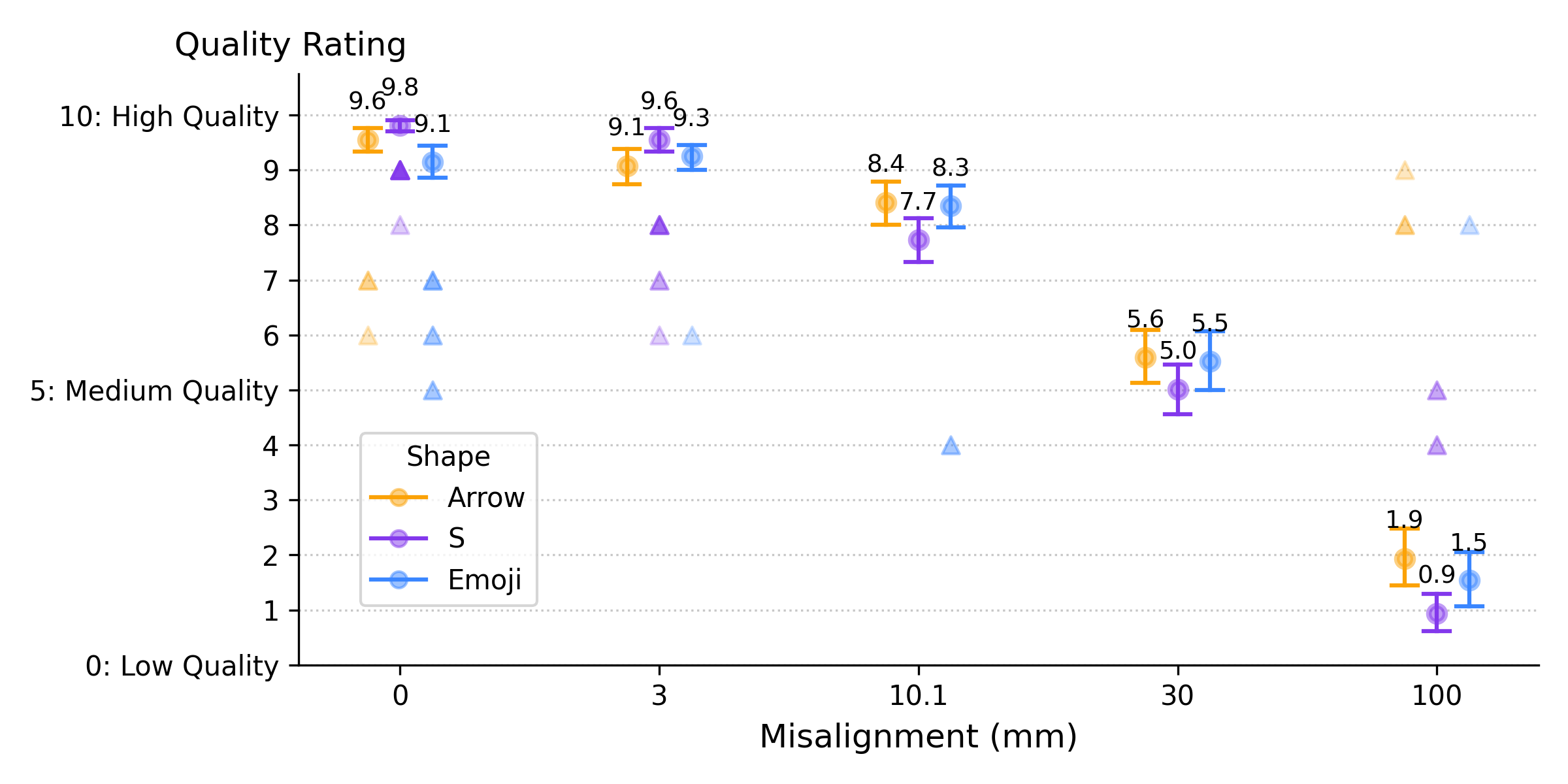
Figure 19 shows the box plot of quality rating (y-axis) as a function of misalignment (x-axis) for each shape. In general, participants’ perceived quality of an illumination decreases as we increased misalignment from 0 to 100 mm. The perceived decrease with a low misalignment of 3 mm is shape dependent. The subjects do not notice it with the Emoji. However, they report a slight decrease in quality with S and Arrow. At a 10.1 mm misalignment, quality ratings is relatively high (mean = 8.16, median = 8), indicating the illuminations are usable. At 30 mm, ratings dropped to medium quality (mean = 5.38, median = 5), denoting noticeable issues with the illumination while still remaining usable. However, at the extreme 100 mm misalignment, perceived quality diminished severely; ratings for the S is less than 1 (completely unusable), while the Arrow and Emoji drops below 2.

A Mann-Whitney U test (Mann and Whitney, 1947) found no significant difference in quality ratings between male and female participants (U = 61.0, p = .698). This lack of gender effect held true across all shapes and all misalignment.

Because our Likert data is ordinal, we evaluated statistical significance using non-parametric Friedman tests (Friedman, 1937) for simple effects, followed by pairwise Wilcoxon signed-rank tests (Wilcoxon, 1945) with Bonferroni corrections for pairwise comparisons. We conducted these test using custom Python scripts and SciPy package (Virtanen et al., 2020).

Effect of misalignment: We found a significant effect of misalignment on quality ratings within all three shapes: Arrow ( $\chi^{2}(4)=76.44,p<.001$ ), Emoji ( $\chi^{2}(4)=73.86,p<.001$ ), and Letter S ( $\chi^{2}(4)=79.49,p<.001$ ).

Post-hoc pairwise comparisons revealed that, despite quality ratings dropping at higher misalignments, users struggle to differentiate between the lowest misalignments. Specifically, for the Arrow, differences between 0 and 3 mm ( $p=.166$ ) and 3 and 10.1 mm ( $p=.069$ ) were not significant. For the Emoji, users did not significantly distinguish between 0 and 3 mm ( $p=1.000$ ) or between 0 and 10.1 mm ( $p=.089$ ). For the ’S’, only the 0 vs. 3 mm comparison was non-significant ( $p=.748$ ). This indicates that for multi-part shapes like the Emoji and Arrow, illuminations with small misalignments ( $\leq 10.1$ ) look almost identical to users, resulting in inconsistent ratings within repeated trials. In contrast, users could more easily detect misalignments beyond 3 mm in the S.

Effect of Shape: We also analyzed how the shape affected quality perception at fixed misalignments. Fridman tests revealed significant differences between the shapes at every error level: 0 mm ( $p<.001$ ), 3 mm ( $p=.004$ ), 10.1 mm ( $p=.031$ ), 30 mm ( $p=.014$ ), and 100 mm ( $p<.001$ ).

Pairwise comparisons show a key insight about shapes. At the 0 mm baseline, the S was rated significantly higher than the Emoji ( $p=.004$ ). This means users easily identified the baseline S as the highest quality, whereas they inconsistently rated the baseline Emoji (not always as the highest quality). At the 100 mm misalignment, the S was rated significantly lower than both the arrow ( $p=0.004$ ) and the Emoji ( $p=0.011$ ). These findings suggest that the continuous geometry of the S makes both its perfect and completely broken states highly obvious to users. In contrast, the multi-part structure of the Arrow and Emoji masks the extreme misalignments, making them harder to consistently judge.

Qualitative Feedback: Participants’ open-ended responses supported our quantitative findings regarding shape geometry. A dominant theme was the distinction between continuous and multi-part shapes. Multiple participants noted that the distortions were more obvious in shapes intended to be single connected component, S, because the misalignment destroyed the continuity (e.g., P1, P11, P19). For the shapes composed of multiple pieces, Emoji and Arrow, one participant reported a ”higher tolerance” (P1) for misalignment. Finally, participants attributed visual stability with higher quality and noted that ”wavering” and ”vibration” degraded the quality (P5, P13, P21).

Table 4. Summary of findings from the human subject study.

Research Question	Summary of Finding
RQ1: Is 10.1 mm acceptable?	Subjects found the 10.1 mm misalignment acceptable (mean = 8.16, median = 8).
RQ2: Do subjects perceive small misalignment compared with no misalignment?	When compared with no misalignment, the perceived decrease in quality at a low misalignment (3 mm) is shape-dependent. Subjects reported a slight decrease with the ‘S’ and Arrow but not with the Emoji; this observation was not statistically significant ^$\dagger$.
RQ3: What misalignment has noticeable issues but is usable?	Illuminations begin to show noticeable visual issues at 30 mm, but are still usable (mean = 5.38, median = 5).
RQ4: Does the shape geometry impact the perceived misalignment?	At both low (e.g., 3 mm) and extreme (e.g., 100 mm) misalignments, the perceived quality is shape-dependent. Shapes with disconnected lines mask misalignments better than those with connected lines.

$\dagger$

This observation is encouraging, as it suggests that minor misalignments do not substantially degrade perceived quality.

9. Conclusions and Future Research

A LightBender is an exciting and emerging area of multimedia research. It is a drone with an actuated LED rod as its lighting primitive. This paper introduced the hardware and software architecture of Figure 2 to author and render illuminations using a swarm of LightBenders. We are extending both the hardware and software in several ways. With the hardware, we are extending the LightBender’s rod to consist of multiple rows of smaller LEDs instead of one row of medium sized LEDs. This will enable us to adjust for the width of the lines when we stagger LightBenders, see discussion of Eq. 10. With the software, we are designing techniques to compute medial axis skeleton (Au et al., 2008; Rodrigues et al., 2018; Lin et al., 2020; Lu et al., 2025) for 3D volumes. We envision an iterative optimization algorithm to adjust the position and the angles of the LightBenders’ rod segments to maximize similarity between the LightBender illumination and the 3D volume. This will include support for animations.

In the longer term, we will investigate techniques that support simultaneous viewing by multiple users from different viewpoints using spatial staggering. We will also explore FLSs (Ghandeharizadeh, 2021) equipped with three-dimensional lighting primitives, such as cubes and pyramids, whose volumetric illuminations complement the line-rendering capabilities of LightBenders.

We will extend our human subject study to focus on the user experience. A key research question is how usable and intuitive is our Blender add-on? This will include participants with and without previous background in the use of Blender, comparing the experiences of the two groups with one another.

We will extend our human-subject study to investigate the user experience of our Blender add-on. In particular, we seek to evaluate its usability and intuitiveness. The study will include participants with and without prior Blender experience, allowing us to compare the experiences of the two groups.

Acknowledgements.

This research is supported by the NSF grant CMMI-2425754. We gratefully acknowledge CloudBank (cloudbank2021) and CloudLab (emulab) for the use of their resources.

References

H. Alimohammadzadeh and S. Ghandeharizadeh (2025) Illuminating English Letters Using a Flying Light Speck. In Proceedings of the 3rd International Workshop on UAVs in Multimedia: Capturing the World from a New Perspective, UAVM ’25, New York, NY, USA. External Links: Link, Document Cited by: §2.
H. Alimohammadzadeh and S. Ghandeharizadeh (2026) Indoor Drone Visual Effects Using LightBenders. In Proceedings of the Special Interest Group on Computer Graphics and Interactive Techniques Conference Posters (SIGGRAPH Posters ’26), SIGGRAPH Posters ’26, New York, NY, USA. External Links: ISBN 979-8-4007-2548-7/2026/07, Link, Document Cited by: §4.
H. Alimohammadzadeh, S. Zhu, J. Bai, and S. Ghandeharizadeh (2024) Reliability Groups with Standby Flying Light Specks. In Proceedings of the 15th ACM Multimedia Systems Conference, MMSys ’24, New York, NY, USA, pp. 1–11. External Links: ISBN 9798400704123, Link, Document Cited by: §6.3.
H. Alimohammadzadeh, S. Zhu, and S. Ghandeharizadeh (2026) Techniques to Conceal Dark Standby Flying Light Specks. ACM Trans. Multimedia Comput. Commun. Appl. 22 (3). External Links: ISSN 1551-6857, Link, Document Cited by: §6.3.
O. K. Au, C. Tai, H. Chu, D. Cohen-Or, and T. Lee (2008) Skeleton Extraction by Mesh Contraction. ACM transactions on graphics (TOG) 27 (3), pp. 1–10. Cited by: §9.
Austin, Patrick (2018) A Record-Breaking Drone Show Ended With Quadcopters Falling from the Sky. Accessed June 19, 2026. [Online]., https://gizmodo.com/a-record-breaking-drone-show-ended-with-quadcopters-fal-1825745673. Cited by: §2.
J. Cardoso and R. José (2012) PuReWidgets: a programming toolkit for interactive public display applications. In Proceedings of the 4th ACM SIGCHI Symposium on Engineering Interactive Computing Systems, EICS ’12, New York, NY, USA, pp. 51–60. External Links: ISBN 9781450311687, Link, Document Cited by: §2.
Y. Erel, O. Kozlovsky-Mordenfeld, D. Iwai, K. Sato, and A. H. Bermano (2024) Casper DPM: Cascaded Perceptual Dynamic Projection Mapping onto Hands. In SIGGRAPH Asia 2024 Conference Papers, SA ’24, New York, NY, USA. External Links: ISBN 9798400711312, Link, Document Cited by: §2.
M. Friedman (1937) The use of ranks to avoid the assumption of normality implicit in the analysis of variance. Journal of the American Statistical Association 32 (200), pp. 675–701. External Links: Document, Link, https://www.tandfonline.com/doi/pdf/10.1080/01621459.1937.10503522 Cited by: §8.2.
S. Ghandeharizadeh (2021) Holodeck: Immersive 3D Displays Using Swarms of Flying Light Specks. In ACM Multimedia Asia, New York, NY, pp. 1–7. External Links: Document Cited by: §1, §2, §9.
S. Ghandeharizadeh (2022) Display of 3D Illuminations using Flying Light Specks. New York, NY, pp. 2996–3005. External Links: ISBN 978-1-4503-9203-7/22/10, Link, Document Cited by: §1, §2.
A. Gomes, C. Rubens, S. Braley, and R. Vertegaal (2016) BitDrones: towards using 3d nanocopter displays as interactive self-levitating programmable matter. In Proceedings of the 2016 CHI Conference on Human Factors in Computing Systems, CHI ’16, New York, NY, USA, pp. 770–780. External Links: ISBN 9781450333627, Link, Document Cited by: §2, §2, §2.
Y. Hirohashi and H. Oku (2025) Aerial display method using a flying screen and long range dynamic projection mapping. IEEE Access 13 (), pp. 62893–62902. External Links: Document Cited by: §2, §2.
H. Hsieh, G. E. Jan, and H. Luo (2023) The Applications and Presentations of Drones in Staged Performances and Contemporary Art. In 2023 IEEE International Conference on e-Business Engineering (ICEBE), Vol. , pp. 281–286. External Links: Document Cited by: §2, §2.
R. Ibrahimov, N. Zherdev, and D. Tsetserukou (2020) DroneLight: Drone Draws in the Air using Long Exposure Light Painting and ML. CoRR abs/2007.15171. External Links: Link, 2007.15171 Cited by: §2, §2.
International Olympic Committee (2020) Spectacular Intel Drone Light Show Helps Bring Tokyo 2020 to Life. Accessed June 19, 2026. [Online]., https://olympics.com/ioc/news/spectacular-intel-drone-light-show-helps-bring-tokyo-2020-to-life-1. Cited by: §2.
M. Iuchi, Y. Hirohashi, and H. Oku (2023) Proposal for an Aerial Display using Dynamic Projection Mapping on a Distant Flying Screen. In 2023 IEEE Conference Virtual Reality and 3D User Interfaces (VR), Vol. , pp. 603–608. External Links: Document Cited by: §2.
[18] JS Bin JS Bin Snippet: nacirij. Note: Accessed June 19, 2026 External Links: Link Cited by: 9(a), 9(a).
Y. Kageyama, D. Iwai, and K. Sato (2024) Efficient Distortion-Free Neural Projector Deblurring in Dynamic Projection Mapping. IEEE Transactions on Visualization and Computer Graphics 30 (12), pp. 7544–7557. External Links: Document Cited by: §2.
R. M. Karp (1972) Reducibility among combinatorial problems. In Complexity of Computer Computations: Proceedings of a symposium on the Complexity of Computer Computations, held March 20–22, 1972, at the IBM Thomas J. Watson Research Center, Yorktown Heights, New York, and sponsored by the Office of Naval Research, Mathematics Program, IBM World Trade Corporation, and the IBM Research Mathematical Sciences Department, R. E. Miller, J. W. Thatcher, and J. D. Bohlinger (Eds.), pp. 85–103. External Links: ISBN 978-1-4684-2001-2, Document, Link Cited by: §6.2.
J. Kim (2010) Within-subjects design. In Encyclopedia of Research Design, pp. 1639–1644. External Links: Document, Link Cited by: §8.
C. Lin, L. Liu, C. Li, L. Kobbelt, B. Wang, S. Xin, and W. Wang (2020) SEG-MAT: 3D Shape Segmentation using Medial Axis Transform. IEEE transactions on visualization and computer graphics 28 (6), pp. 2430–2444. Cited by: §9.
R. Lingamaneni, T. Kubitza, and J. Scheible (2017) DroneCAST: Towards a Programming Toolkit for Airborne Multimedia Display Applications. In Proceedings of the 19th International Conference on Human-Computer Interaction with Mobile Devices and Services, MobileHCI ’17, New York, NY, USA. External Links: ISBN 9781450350754, Link, Document Cited by: §2.
C. R. Ltd (2026) Skybrush software. Note: Accessed June 19, 2026 External Links: Link Cited by: §2, §2.
J. Lu, Y. Liang, H. Han, J. Hua, J. Jiang, X. Li, and Q. Huang (2025) A Survey on Computational Solutions for Reconstructing Complete Objects by Reassembling their Fractured Parts. In Computer Graphics Forum, Vol. 44, pp. e70081. Cited by: §9.
Lumasky Drone Shows (2023) 1,500 Drone Show to Illuminate the Story of Khaybar. Accessed June 19, 2026. [Online]., https://lumasky.show/projects/1500-drone-show-to-illuminate-the-story-of-khaybar/. Cited by: §2.
H. B. Mann and D. R. Whitney (1947) On a Test of Whether one of Two Random Variables is Stochastically Larger than the Other. The Annals of Mathematical Statistics 18 (1), pp. 50 – 60. External Links: Document, Link Cited by: §8.2.
T. Nomoto, W. Li, H. Peng, and Y. Watanabe (2022) Dynamic Multi-projection Mapping Based on Parallel Intensity Control. IEEE Transactions on Visualization and Computer Graphics 28 (5), pp. 2125–2134. External Links: Document Cited by: §2.
H. Nozaki (2014) Flying Display: A Movable Display Pairing Projector and Screen in the Air. In CHI ’14 Extended Abstracts on Human Factors in Computing Systems, CHI EA ’14, New York, NY, USA, pp. 909–914. External Links: ISBN 9781450324748, Link, Document Cited by: §2.
S. Oh, S. Kang, K. Lee, S. Ahn, and E. Kim (2006) Flying Display: Autonomous Blimp with Real-Time Visual Tracking and Image Projection. In 2006 IEEE/RSJ International Conference on Intelligent Robots and Systems, Vol. , pp. 131–136. External Links: Document Cited by: §2.
H. Peng and Y. Watanabe (2021) High-Speed Dynamic Projection Mapping onto Human Arm with Realistic Skin Deformation. Applied Sciences 11 (9). External Links: Link, ISSN 2076-3417, Document Cited by: §2.
J. Preiss, W. Hoenig, N. Ayanian, and G. Sukhatme (2017) Downwash-Aware Trajectory Planning for Large Quadcopter Teams. IEEE/RSJ International Conference on Intelligent Robots and Systems (IROS), pp. 8. Cited by: §1, §7.
R. S. Rodrigues, J. F. Morgado, and A. J. Gomes (2018) Part-Based Mesh Segmentation: A Survey. In Computer Graphics Forum, Vol. 37, pp. 235–274. Cited by: §9.
J. Scheible, A. Hoth, J. Saal, and H. Su (2013) Displaydrone: a flying robot based interactive display. In Proceedings of the 2nd ACM International Symposium on Pervasive Displays, PerDis ’13, New York, NY, USA, pp. 49–54. External Links: ISBN 9781450320962, Link, Document Cited by: §2.
J. Scheible, R. Lingamaneni, and M. Funk (2019) DisplayDrone as Police Deployment Tool for Ubiquitously Available Public Displays and Digital Signage. External Links: Link Cited by: §2, §2, §2.
S. Schneegass, F. Alt, J. Scheible, A. Schmidt, and H. Su (2014a) Midair displays: exploring the concept of free-floating public displays. In CHI ’14 Extended Abstracts on Human Factors in Computing Systems, CHI EA ’14, New York, NY, USA, pp. 2035–2040. External Links: ISBN 9781450324748, Link, Document Cited by: §2, §2.
S. Schneegass, F. Alt, J. Scheible, and A. Schmidt (2014b) Midair displays: concept and first experiences with free-floating pervasive displays. In Proceedings of The International Symposium on Pervasive Displays, PerDis ’14, New York, NY, USA, pp. 27–31. External Links: ISBN 9781450329521, Link, Document Cited by: §2, §2.
S. Schneegass and F. Alt (2014) SenScreen: a toolkit for supporting sensor-enabled multi-display networks. In Proceedings of The International Symposium on Pervasive Displays, PerDis ’14, New York, NY, USA, pp. 92–97. External Links: ISBN 9781450329521, Link, Document Cited by: §2.
V. Serpiva, E. Karmanova, A. Fedoseev, S. Perminov, and D. Tsetserukou (2021) DronePaint: Swarm Light Painting with DNN-based Gesture Recognition. New York, NY, USA. External Links: ISBN 9781450383646, Link, Document Cited by: §2, §2.
Sky Elements Drone Shows (2023) Sky Elements Ignites the NCAA Mens Final Four with an Electrifying Texas Drone Light Show! Accessed June 19, 2026. [Online]., https://skyelementsdrones.com/drone-events/sky-elements-ignites-the-ncaa-mens-final-four-with-an-electrifying-texas-drone-light-show/. Cited by: §2.
SPH Engineering (2024) The Growing Trend of Integrated Drones and Fireworks Shows., https://www.droneshowsoftware.com/news/the-growing-trend-of-integrated-drones-and-fireworks-shows. Note: Accessed June 19, 2026 Cited by: §2.
SPH Engineering (2026) Drone show software. Note: Accessed June 19, 2026 External Links: Link Cited by: §2, §2.
Y. Su, C. Chu, M. Wang, J. Li, L. Yang, Y. Zhu, and H. Liu (2022) Downwash-aware Control Allocation for Over-actuated UAV Platforms. In 2022 IEEE/RSJ International Conference on Intelligent Robots and Systems (IROS), Vol. , pp. 10478–10485. External Links: Document Cited by: §1.
G. M. Sullivan and A. R. Jr. Artino (2013) Analyzing and Interpreting Data From Likert-Type Scales. Journal of Graduate Medical Education 5 (4), pp. 541–542. External Links: Document Cited by: §8.
H. Tobita, S. Maruyama, and T. Kuzi (2011) Floating Avatar: Telepresence System using Blimps for Communication and Entertainment. In CHI ’11 Extended Abstracts on Human Factors in Computing Systems, CHI EA ’11, New York, NY, USA, pp. 541–550. External Links: ISBN 9781450302685, Link, Document Cited by: §2.
D. Tone, D. Iwai, S. Hiura, and K. Sato (2020) FibAR: Embedding Optical Fibers in 3D Printed Objects for Active Markers in Dynamic Projection Mapping. IEEE Transactions on Visualization and Computer Graphics 26 (5), pp. 2030–2040. External Links: Document Cited by: §2.
Verge Aero (2026) Design studio software. Note: Accessed June 19, 2026 External Links: Link Cited by: §2, §2.
Verity Studios and ETH Zurich and Cirque du Soleil (2016) SPARKED: A Live Interaction Between Humans and Quadcopters. Accessed June 19, 2026. [Online]., https://starts-prize.aec.at/en/sparked/. Cited by: §2.
P. Virtanen, R. Gommers, T. E. Oliphant, M. Haberland, T. Reddy, D. Cournapeau, E. Burovski, P. Peterson, W. Weckesser, J. Bright, S. J. van der Walt, M. Brett, J. Wilson, K. J. Millman, N. Mayorov, A. R. J. Nelson, E. Jones, R. Kern, E. Larson, C. J. Carey, İ. Polat, Y. Feng, E. W. Moore, J. VanderPlas, D. Laxalde, J. Perktold, R. Cimrman, I. Henriksen, E. A. Quintero, C. R. Harris, A. M. Archibald, A. H. Ribeiro, F. Pedregosa, P. van Mulbregt, and SciPy 1.0 Contributors (2020) SciPy 1.0: Fundamental Algorithms for Scientific Computing in Python. Nature Methods 17, pp. 261–272. External Links: Document Cited by: §8.2.
F. Wilcoxon (1945) Individual comparisons by ranking methods. Biometrics Bulletin 1 (6), pp. 80–83. External Links: ISSN 00994987, Link Cited by: §8.2.
W. Yamada, K. Yamada, H. Manabe, and D. Ikeda (2017) ISphere: self-luminous spherical drone display. In Proceedings of the 30th Annual ACM Symposium on User Interface Software and Technology, UIST ’17, New York, NY, USA, pp. 635–643. External Links: ISBN 9781450349819, Link, Document Cited by: §2, §2.
N. Yazdani and S. Ghandeharizadeh (2025) Integration of 3D FLS Displays with 3D Authoring Tools. New York, NY. External Links: ISBN 79-8-4007-2051-2/2025/10, Link, Document Cited by: §7.
H. Yoon, W. Wan, H. Kim, N. Hovakimyan, L. Sha, and P. G. Voulgaris (2019) Towards Resilient UAV: Escape Time in GPS Denied Environment with Sensor Drift. IFAC-PapersOnLine 52 (12), pp. 423–428. Note: 21st IFAC Symposium on Automatic Control in Aerospace ACA 2019 External Links: ISSN 2405-8963, Document, Link Cited by: §1.
A. You, J. Li, Z. Xu, and W. Liu (2021) Design of Entertainment Drone with Rotating LED Display Technology. Journal of Physics: Conference Series 2113 (1), pp. 012058. External Links: Document, Link Cited by: §2.

Appendix A Blender add-on and LED Color Expressions

Once an artist places a LightBender in Blender’s 3D viewport using our add-on, they may specify LED illumination using expressions over the two segments of its actuated rod. A pointer consists of an index and a color expression. For the 160 mm LightBender, LEDs are indexed from 0 to 49. An expression is evaluated for a range of LEDs and may produce a color dependent on time. The range is specified using a pair of consecutive pointers. A single LED at index $i$ is identified by the range [ $i$ , $i+1$ ). Figure 20 shows three examples. First, bottom right hand side of the figure shows an expression to turn the range of LEDs [0,15) off by setting their color values to black, RGB $(0,0,0)$ . Second, an expression may assign the same color to all LEDs in a range to display a solid color. The expression with RGB $(10,100,30)$ and range [15, 35) results in solid green in the middle of rod, see Figure 20. It is used to illuminate the uniform green of the arrow in Figure 1. Third, an expression may define a color gradient for an LED range. An example is range [35, 50) with $(i-35)*15$ in Figure 20. In this case, the LEDs transition smoothly between two colors throughout the range of the 15 LEDs. Blue to red in Figure 20. The color of each LED is interpolated linearly from the start color to the end color on the basis of its position. This expression type is used to create smooth color transitions along a rod segment.