WingSpan: Concurrency and Dependence for Sparse and Structured Tensor Compilers

Adrian Gushin Georgia Institute of TechnologyAtlantaGeorgiaUSA agushin3@gatech.edu , Sang Yoon Kim Georgia Institute of TechnologyAtlantaGeorgiaUSA sangyoon@gatech.edu and Willow Ahrens Georgia Institute of TechnologyAtlantaGeorgiaUSA ahrens@gatech.edu

Abstract.

Sparse tensors represent data that is mostly zero or some other compressible fill pattern. Such datasets can be massive, so optimized tensor algebra libraries and compilers have been developed to exploit these patterns to improve performance. Existing systems, however, frequently lack support for parallelism, especially when outputs are sparse or multiple inputs are sparse. We propose WingSpan, a sparse tensor language enabling unrestricted parallel programming. WingSpan supports arbitrary composition of parallel loops and data structures, matching or exceeding the performance of hand-optimized parallel routines on critical kernels such as SpGEMM. We also introduce a dependence theory for the safety of parallel programs involving sparse tensors and structures beyond sparsity.

Sparse Tensors, Parallel, Programming Languages

^†^†copyright: none

1. Introduction

Datasets in the modern era have become massive, but many tensors contain patterns allowing for compressed representations that make computation tractable. Sparse tensors contain mostly zero or “fill” values; additional patterns, such as non-zero blocks or identical-value runs, enable further compression (donenfeld_unified_2022). Sparsity occurs naturally in real-world applications with community structure, such as graph algorithms (kepner_graph_2011), quantum simulations (venev_qblaze_2025), or neural networks (zhu_survey_2024; frankle_lottery_2019). Efficient sparse kernels are essential to handle these applications at scale (de2019deep; hochbaum2016sparse; el2013understanding; jenkinson2014machine).

Optimizing sparse applications can be complex. Due to algebraic properties like $x*0=0$ , only nonfill values must be stored and processed. However, operating directly on compressed data structures involves intricate traversals and invariants. To address this complexity, a variety of compiler approaches have emerged to automatically generate efficient kernels. Frameworks such as TACO, Finch, and SparseTIR support a wide range of data structures, hardware architectures, and optimizations (kjolstad_taco_2017; ahrens_finch_2025; chou_format_2018; ye_sparsetir_2023; bik_compiler_2022).

Among parallel targets, multicore CPUs are critical for sparse compilers. CPU-exclusive supercomputers like Fugaku compete for first place globally when evaluated on sparse benchmarks like the Graph500 (graph500). CPU performance is key to enabling compute-intensive tasks, like mobile computer vision, on edge and embedded devices (kong2025simulating). Finally, sparse kernels like SpGEMM involve extensive control flow, making CPUs a natural target for their highly optimized branch predictors and management logic (won2026insum).

Unfortunately, existing sparse tensor compiler support for parallelism is limited and fragmented. TACO, for example, only supports parallelism when the output is dense, and can only load balance effectively when only one input is sparse (senanayake_sparse_2020). MLIR Sparse supports sparse outputs by creating a large temporary buffer full of each individual summand together with its coordinate, then sorts and sums them later (bik_compiler_2022). Other compilers, such as Taichi or SparseTIR, have similar constraints (hu_taichi_2019; ye_sparsetir_2023). All of these systems require intricate manual tuning to achieve good performance.

There are several challenges in parallel sparse algorithms:

Complex Data Structure Invariants: Sparse data structures are complex, interdependent, and difficult to update concurrently. Even the most common formats, such as CSR, involve prefix sums and large contiguous data buffers. Taking Figure 2 as an example, several formats have complex nested structures that require careful synchronization to update safely in parallel. Algorithms may parallelize along different data structure dimensions with different dependence guarantees. Sparse parallel programming paradigms must therefore safely access these complex structures without breaking critical invariants. Doing so while maintaining scalability across multiple cores is a central challenge.

Irregular Compute Balance: Sparse workloads are often imbalanced. When a single input is sparse, the non-zeroes can be treated as proportional to the work (senanayake_sparse_2020). However, when multiple inputs are sparse, the amount of work per non-zero is not easily statically computable and can vary significantly at runtime (dasgupta_sparse_2012). Dynamic load balancing would be an effective strategy to scale with near-optimal efficiency, but computing dynamic pieces of a sparse output directly is a challenge, and existing compilers do not support it.

Weak Theoretical Foundation: Dependence analysis verifies the safety of compiler optimizations in dense code, such as tiling and parallelization, by assuming that distinct coordinate tuples imply isolated memory locations (kennedy2001optimizing). For example, threads modifying $A[1,1]$ and $A[2,1]$ cannot race because $(1,1)\neq(2,1)$ . This assumption fails in sparse formats, where distinct indices may share indirection arrays or depend on cumulative sums. New theoretical tools are necessary to safely parallelize sparse tensor programs.

To address these challenges, we present WingSpan, a high-level parallel array programming language for sparse tensor algebra that compiles to performant LLVM code. Existing sparse tensor compilers such as TACO or Finch can describe sparse and structured data hierarchically, associating each dimension with a level in a tree annotated with format descriptors. These descriptors denote the level’s data representation, such as dense or sparse. Finch is notable for supporting a surprising variety of formats, including block and run-length encoded levels. WingSpan builds on Finch to make the following three contributions:

1. Concurrent annotations for Finch’s hierarchical sparse tensor format description language. We add the mutex, shard, and merge level wrappers, diagrammed in Figure LABEL:fig:parallel-levels. We build the first compiler that supports parallel sparse outputs directly, without intermediates. WingSpan’s new formats extend and interoperate with the entire existing format language to facilitate parallelism.

2. A sparsity-aware parallel programming language, supporting nested parallelism, parallelism around and within sparse workspaces, and static and dynamic scheduling. Ours is the first language to support arbitrary composition of parallel loops, and the first to support arbitrary interactions between parallel loops and sparse workspaces. Our abstraction comes at no cost to performance; we match or exceed state-of-the-art parallel systems on tensor applications like SpGEMM ( $1.21\times$ geomean speedup), SpAdd ( $4.22\times$ ), Hadamard product ( $3.39\times$ ), SpMSpV ( $1.47\times$ ), and MTTKRP ( $0.96\times$ ).

3. The first dependence theory of parallel programming safety for hierarchical sparse and structured tensor formats. Our theory accounts for all of the dense, sparse, and otherwise structured tensor descriptions in Finch’s language, which is to our knowledge the largest set of such formats (ahrens_finch_2025). Our new theoretical foundation enables developers to prove their algorithm parallelizes without race conditions regardless of the tensor types used in the program.

2. Background

2.1. Fiber Trees

Fiber-tree style tensor abstractions for sparse and structured data are abundant (sze_efficient_2020; chou_compilation_2022; chou_format_2018). Fiber-trees represent a multi-dimensional tensor as a nested vector structure, where each level of the nesting corresponds to a dimension of the tensor. For example, a matrix would be represented as a vector of vectors. Fiber-trees can represent sparse tensors by varying the format of vectors used at each level in a tree. Thus, a CSC sparse matrix might be represented as a dense vector of sparse vectors. Nodes in the tree are referred to as fibers.

Refer to caption — Figure 1. A fiber tree representation of a sparse matrix in CSC format, with a dense outer level, a sparse inner level, and an element level of leaves that store values (ahrens_finch_2025; sze_efficient_2020). Note that each index within a level’s fibers maps to a position in its child level. When the child is a leaf, this map materializes directly to a payload (value).

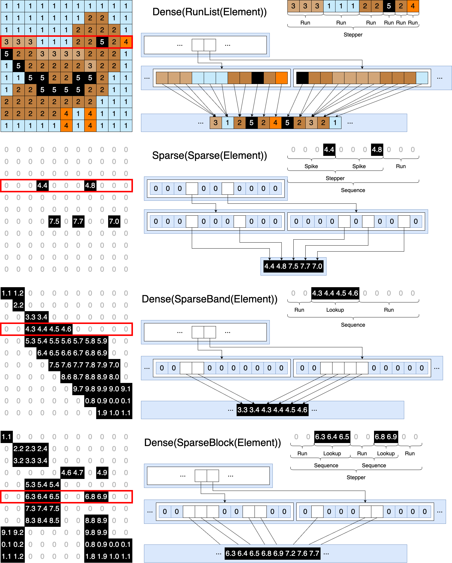
Instead of storing the data for each subfiber separately, most sparse tensor formats, such as CSR, DCSR, and COO, usually store the data for all fibers in a level contiguously. In this way, we can think of a level as a bulk allocator for fibers. Continuing the analogy, each fiber is disambiguated by a position, or an identifier in the bulk pool of subfibers. When we need to refer to a particular fiber $f$ at position $p$ in level $l$ of tensor $T$ , we may write $f=\texttt{fiber}(T,l,p)$ . Figure 1 shows a simple example of a level as a pool of fibers. The children of fibers can be addressed with indices, expressible as $f(i)$ . If the child is a subfiber at position $q$ , then $f(i)=\texttt{child}(q)$ . If the child is a constant $z$ , such as zero, then $f(i)=\texttt{payload}(z)$ .

2.2. Finch Tensor Compiler

Finch, a state-of-the-art tensor compiler, is unique for its great diversity of level formats (ahrens_finch_2025). It extends level-by-level fibertree descriptions to capture any combination of banded, triangular, run-length-encoded, padding, one-hot-encoding, or sparse datasets, as shown in Figure 2.

WingSpan uses the Finch compiler to support lowering to LLVM code. Particularly, it exploits Finch’s hierarchical tensor decomposition to integrate the modifier levels shown in Figure LABEL:fig:parallel-levels. We refer to WingSpan’s levels as modifiers to emphasize that, unlike standard levels, they are dimensionless. Rather, they construct the data structures and code lowering algorithms necessary to parallelize Finch code.

WingSpan’s strategy is sufficiently general that it could be implemented using any state-of-the-art tensor compiler with hierarchical formats, such as TACO. We use Finch because it supports the greatest diversity in physical level formats. WingSpan’s modifier levels interoperate with any permutation of child levels, so Finch’s greater format diversity maximizes the language’s expressive power. This flexibility enables WingSpan to parallelize a larger number of kernels across a larger combination of tensor storage choices.

Because WingSpan builds atop of Finch, our code is integrated into the larger Finch compiler. The entire system is available online at the Finch GitHub repository. ¹¹1”Wingspan is merged to main in the Finch repository, available online at https://github.com/finch-tensor/Finch.jl. We also provide our harness for our performance section. ²²2Our benchmark harness is available online at https://github.com/finch-tensor/FinchBenchmarks/tree/cgo26-artifact.

2.3. Classical Dependence Analysis

Safe parallel code requires avoiding race conditions. Classical dependence analysis can determine when it is possible to safely transform or parallelize loops over dense arrays(kennedy2001optimizing).

To introduce vocabulary, consider an $n$ -dimensional tensor $A$ mapping $n$ -tuples of integer coordinates to values. The access expression $A_{ijk\cdots}$ refers to the value stored at a particular location $ijk...$ . The terms $i,j,k...$ may be expressions and are referred to as tensor indices or subscripts. We refer to the loop iteration variable as a loop index. For example, in the loop “for i in 1:m”, $i$ is the loop index. In the style of Fortran, we index from 1 and assume column-major order, so the first subscript of a tensor has unit stride.

We say that two accesses are dependent if one of them is a write and they access the same memory location, and independent otherwise. Dependence extends to multidimensional tensors by requiring that all subscripts match pairwise across the two accesses. A dependence may occur between an access expression and itself in different loop iterations, or between two accesses in the same iteration. Independence requires that no two loop iterations access the vector at the same subscript value, which implies that there is no distribution of iterations to threads that could cause a data race. Figure 3 gives a simple example.

⬇

for i=parallel(_)

c[i] += 1

end

⬇

for i=parallel(_)

c[i - i end

Figure 3. Two example kernels. The access is independent on the left because no two loop iterations will modify

c

with the same value for

i

. Thus, the kernel is safe to parallelize. The access on the right is dependent on itself since adjacent loop iterations modify the same element of

c

. This potential race means that the kernel may not be safe to parallelize.

Two different kernels accessing a vector c. The first iterates over all of c’s values in parallel, with each iteration incrementing c at index i by 1. The second is similar, but pairs up adjacent iterations by accessing c at i minus i mod 2. The first kernel is independent because no two iterations of the loop will access c using the same value for c. In the second, i is dependent because adjacent loop iterations access c using the same value

3. Level Dependence Testing

The foundational assumption undergirding classical dependence analysis is that distinct subscript tuples refer to distinct memory locations. This assumption holds for dense tensors because they map directly to contiguous memory regions. However, unlike dense arrays, sparse arrays are stored in tree structures built from multiple levels. Materializing a single coordinate results in multiple memory operations across different levels of the tensor tree. Figure 4 shows that seemingly independent accesses can result in collisions in fibertrees. Reasoning about dependence in the sparse case therefore requires examining each level of the tree separately.

3.1. Dependencies on Tensor Trees

Classical dependence can be generalized to tree structures through node dependence. Two subscript tuples are level- $k$ node dependent on tensor A if they access the same memory location on level $k$ of the fibertree. The language of classical theory is sufficient to capture this nuance. For a level $k$ in a leaf-to-root path $k,\cdots,q,p$ , the subscript accessing $k$ is $(k,\cdots,q,p)$ . For example, in Figure 4, level 1 is accessed by subscript $j$ and level 2 by $(i,j)$ . Using a dependence test like Banerjee’s inequality on level $k$ ’s subscript can detect a level- $k$ node dependence (banerjee1997dependence). Therefore, using these tests on every level’s access subscript will compute the set of all node dependencies on the tree. In Figure 4, testing subscript $j$ would detect the level-1 node dependence from the race on $j=1$ , and disprove level-2 node dependence because its subscript $(i,j)$ is always accessed with unique pairs.

While node dependence begins to generalize the language of dependence analysis to tensor tree representations, it is not complete. Sparse and structured levels are often composed of complex data buffers with invariants that can be violated even if parallel accesses occur at different nodes. For instance, the compressed sparse column format uses several buffers maintaining cumulative prefix sums that must remain monotonically non-decreasing (chou_format_2018). Otherwise safe parallel updates to these arrays could induce data races by inadvertently violating these invariants.

The presented sparse representations are merely a single problem case. There are myriad other tensor format descriptors, each of which has idiosyncratic invariants. Writing a separate dependency theory for each one is not feasible. We generalize by analyzing the three types of level dependencies parallel accesses can create. To introduce these definitions, recall from Section 2.1 that levels are pools of fibers, and the fiber at position $p$ in level $l$ in tensor $T$ is denoted as $f=\texttt{fiber}(T,l,p)$ and can be accessed at index $i$ as $f(i)$ .

Under this construction, a parallel dependence between two fiber accesses $\texttt{fiber}(T,k,p)(i)$ and $\texttt{fiber}(T,k,p^{\prime})(i^{\prime})$ in level $k$ can be categorized into three types:

•

Level- $k$ node dependence if the accesses modify the same fiber and the same index, $p^{\prime}=p$ and $i^{\prime}=i$ .
•

Level- $k$ sibling dependence if the accesses modify the same fiber with different indices, $p=p^{\prime}$ and $i\neq i^{\prime}$ .
•

Level- $k$ cousin dependence if the accesses are made to different fibers, $p\neq p^{\prime}$ .

This vocabulary allows for greater precision when discussing level dependencies. For example, in Figure 4, the black and red accesses to $(2,1)$ and $(3,1)$ create a level-1 node dependence and a level-2 sibling dependence. Similarly, the red and orange accesses to $(3,1)$ and $(2,2)$ produce a level-1 sibling and a level-2 cousin dependence.

Different levels have different representations, some of which can safely support these access patterns. To track these safety guarantees while maintaining generality, each tensor has a stability vector $S$ . For an $n$ -mode tensor, $S$ is a vector of $n+1$ sets. $S_{1}$ represents the tensor’s leaf (element) level, and every subsequent entry corresponds to a mode in the tensor. For a mode $k$ , $S_{k+1}$ is the subset of $\{$ node, sibling, cousin $\}$ dependencies that the level representing $k$ ’s dimension can support without causing undefined behavior.

A

\triangleright

The tensor to be accessed

S

\triangleright

A’s stability vector.

p

\triangleright

The loop we wish to parallelize

f_{1}(i...),...,f_{m}(i...)

\triangleright

Subscripts of first access

g_{1}(i^{\prime}...),...,g_{m}(i^{\prime}...)

\triangleright

Subscripts of second access

i...

the indices of loops within the scope of

A

’s declaration which contain both accesses, from root to leaf.

for

j=1,...,m+1

d\leftarrow\mathop{dep\_test}((f_{j}(i...),...,f_{m}(i...)),

\hskip 45.00006pt(g_{j}(i^{\prime}...),...,g_{m}(i^{\prime}...)))

race_{position}=d_{1},...,d_{p-1}\in\{=,*\}\text{ and }d_{p}\not\in\{=\}

j>1

then

d^{\prime}\leftarrow\mathop{dep\_test}((f_{j-1}(i...),...,f_{m}(i...)),

\hskip 45.00006pt(g_{j-1}(i^{\prime}...),...,g_{m}(i^{\prime}...)))

race_{index}=d^{\prime}_{1},...,d^{\prime}_{p-1}\in\{=,*\}\text{ and }d^{\prime}_{p}\not\in\{=\}

end if

W_{j}\leftarrow\varnothing

i_{p}\not\in f_{j},...f_{m},g_{j},...,g_{m}

and

i_{p}\in f_{1}...f_{m},g_{1},...g_{m}

then

continue

\triangleright

Skip levels not accessed in parallel

end if

if not

race_{position}

then

W_{j}\leftarrow W_{j}\cup\text{\{cousin\}}

end if

race_{position}

and not

race_{index}

then

W_{j}\leftarrow W_{j}\cup\text{\{sibling, cousin\}}

end if

race_{index}

then

W_{j}\leftarrow W_{j}\cup\text{\{node, sibling, cousin\}}

end if

end for

return

W

Algorithm 1 A dependence test for a single pair of accesses. The algorithm returns

W

, the required stability for each level of the tensor. Note that

race_{position}

is true when there is a possible race on the position of the level, and

race_{index}

is true when there is a possible race on both the position and index. The access pair is safe if

W_{j}\subseteq S_{j}

for all

j

The lack of stability in Finch’s existing level formats reveals the difficulty in sparse parallelism. Element (leaf) levels have no children, but cannot support data races on the leaves, so $S_{1}=\{$ sibling, cousin $\}$ . Additionally, if $m$ ’s level is dense, $S_{m+1}=\{$ node, sibling, cousin $\}$ because dense levels are static mapping functions. Unfortunately, for any other level format, $S_{m+1}=\varnothing$ . WingSpan enables sparse and structured parallelism by addressing this gap.

3.2. The Level Dependence Test

Dependence tests can detect data races on a dense multidimensional array. In this section, we expand such tests to handle trees. Let $i=(i_{1},...,i_{n})$ be the vector of values of loop indices in a loop nest. A standard dependence test determines whether (and when) two accesses $A_{f_{1}(i...),...,f_{m}(i...)}$ in iteration $i$ and $A_{g_{1}(i^{\prime}...),...,g_{m}(i^{\prime}...)}$ in iteration $i^{\prime}$ access the same memory. The result is a direction vector $d$ representing the constraints $i_{k}d_{k}i^{\prime}_{k}$ , where $d_{k}\in\{<,=,>,*\}$ . The $*$ value indicates there is no provable constraint on $i_{k}$ and $i^{\prime}_{k}$ .

A loop is safe to parallelize if it does not carry a dependence. Loop $p$ carries a dependence when $d_{1}...d_{p}-1$ are in $\{*,=\}$ and $d_{p}$ is not $=$ . If these conditions are true, the parallel loop generates repeated subscripts across multiple iterations. Consequently, different iterations of the same parallel loop might access the same array element and a race condition is possible. We conservatively include $*$ in the check on $d_{1}...d_{p-1}$ because $*$ does not disprove a $=$ relationship.

Algorithm 1 builds on this notion to determine when the tensor’s stability is sufficient for a particular parallel loop. The algorithm computes a loop nest’s direction vector and uses the properties of loop carried dependencies to determine the types of parallel accesses a program will make to a tensor. Running Algorithm 1 against all subscript pairs and parallel loops in a program evaluates whether a tensor’s stability vector is sufficient to prevent race conditions in the program.

4. The WingSpan Language

	$\displaystyle T\in\text{Tensor}$	$\displaystyle\qquad l,p,a,b,n,c\in\mathbb{Z}\qquad v\in\text{Literal}\qquad i\in\text{Index}\qquad\sigma\in\text{Store}$
	$\displaystyle x,y\in$	$\displaystyle\text{Variable}\qquad t\in\mathchoice{\hbox{\pagecolor{dev1green}$\displaystyle\text{Task}$}}{\hbox{\pagecolor{dev1green}$\textstyle\text{Task}$}}{\hbox{\pagecolor{dev1green}$\scriptstyle\text{Task}$}}{\hbox{\pagecolor{dev1green}$\scriptscriptstyle\text{Task}$}}\qquad D\in\mathchoice{\hbox{\pagecolor{dev1green}$\displaystyle\text{Device}$}}{\hbox{\pagecolor{dev1green}$\textstyle\text{Device}$}}{\hbox{\pagecolor{dev1green}$\scriptstyle\text{Device}$}}{\hbox{\pagecolor{dev1green}$\scriptscriptstyle\text{Device}$}}\qquad h\in\mathchoice{\hbox{\pagecolor{dev1green}$\displaystyle\text{Schedule}$}}{\hbox{\pagecolor{dev1green}$\textstyle\text{Schedule}$}}{\hbox{\pagecolor{dev1green}$\scriptstyle\text{Schedule}$}}{\hbox{\pagecolor{dev1green}$\scriptscriptstyle\text{Schedule}$}}$
	$\displaystyle C\in\text{Context}$	$\displaystyle::=\langle s,t,\sigma\rangle\qquad m\in\text{Mode}::=\begin{aligned} &\texttt{read}\mid\texttt{update}(\oplus)\mid\texttt{undeclared}\end{aligned}$
	$\displaystyle A\in\text{Access}$	$\displaystyle::=\texttt{access}(F,i\ldots)\qquad F\in\text{Fiber}::=\texttt{fiber}(T,l,p)$
	$\displaystyle e\in\text{Expression}$	$\displaystyle::=\begin{aligned} &v\mid\texttt{call}(\otimes,e_{1},\ldots,e_{n})\mid\texttt{access}(F,i\ldots)\end{aligned}$
	$\displaystyle r\in\text{Range}$	$\displaystyle::=a\texttt{:}b\mid\texttt{looplet}(a\texttt{:}b)\mid\mathchoice{\hbox{\pagecolor{dev1green}$\displaystyle\texttt{parallel}(r,D,h)$}}{\hbox{\pagecolor{dev1green}$\textstyle\texttt{parallel}(r,D,h)$}}{\hbox{\pagecolor{dev1green}$\scriptstyle\texttt{parallel}(r,D,h)$}}{\hbox{\pagecolor{dev1green}$\scriptscriptstyle\texttt{parallel}(r,D,h)$}}$
	$\displaystyle s\in\text{Statement}$	$\displaystyle::=s_{1};s_{2}\mid\texttt{if}(e,s)\mid\mathchoice{\hbox{\pagecolor{dev1green}$\displaystyle s_{1}\\|s_{2}$}}{\hbox{\pagecolor{dev1green}$\textstyle s_{1}\\|s_{2}$}}{\hbox{\pagecolor{dev1green}$\scriptstyle s_{1}\\|s_{2}$}}{\hbox{\pagecolor{dev1green}$\scriptscriptstyle s_{1}\\|s_{2}$}}\mid C\mid x\texttt{=}e\mid\texttt{assign}(A,\oplus,e)\mid\texttt{skip}$
		$\displaystyle\mid\texttt{unwrap}(F)\mid\texttt{increment}(F,\oplus,e)\mid\texttt{unfurl}(F)$
		$\displaystyle\mid\texttt{declare}(T,z,\oplus,n\ldots)\mid\texttt{freeze}(T,\oplus)\mid\texttt{thaw}(T,\oplus)$
		$\displaystyle\mid\mathchoice{\hbox{\pagecolor{dev1green}$\displaystyle\texttt{spawn}(s,D,e)$}}{\hbox{\pagecolor{dev1green}$\textstyle\texttt{spawn}(s,D,e)$}}{\hbox{\pagecolor{dev1green}$\scriptstyle\texttt{spawn}(s,D,e)$}}{\hbox{\pagecolor{dev1green}$\scriptscriptstyle\texttt{spawn}(s,D,e)$}}\mid\mathchoice{\hbox{\pagecolor{dev1green}$\displaystyle\texttt{transfer}(T,s)$}}{\hbox{\pagecolor{dev1green}$\textstyle\texttt{transfer}(T,s)$}}{\hbox{\pagecolor{dev1green}$\scriptstyle\texttt{transfer}(T,s)$}}{\hbox{\pagecolor{dev1green}$\scriptscriptstyle\texttt{transfer}(T,s)$}}\mid\texttt{for}\ i=r\ \texttt{do}\ s\ \texttt{end}$
		$\displaystyle\mid\mathchoice{\hbox{\pagecolor{dev1green}$\displaystyle\texttt{worker}(i,r,h,s)$}}{\hbox{\pagecolor{dev1green}$\textstyle\texttt{worker}(i,r,h,s)$}}{\hbox{\pagecolor{dev1green}$\scriptstyle\texttt{worker}(i,r,h,s)$}}{\hbox{\pagecolor{dev1green}$\scriptscriptstyle\texttt{worker}(i,r,h,s)$}}\mid\mathchoice{\hbox{\pagecolor{dev1green}$\displaystyle\texttt{checkout}(T,l,m,t)$}}{\hbox{\pagecolor{dev1green}$\textstyle\texttt{checkout}(T,l,m,t)$}}{\hbox{\pagecolor{dev1green}$\scriptstyle\texttt{checkout}(T,l,m,t)$}}{\hbox{\pagecolor{dev1green}$\scriptscriptstyle\texttt{checkout}(T,l,m,t)$}}\mid\mathchoice{\hbox{\pagecolor{dev1green}$\displaystyle\texttt{commit}(T,l,m,t)$}}{\hbox{\pagecolor{dev1green}$\textstyle\texttt{commit}(T,l,m,t)$}}{\hbox{\pagecolor{dev1green}$\scriptstyle\texttt{commit}(T,l,m,t)$}}{\hbox{\pagecolor{dev1green}$\scriptscriptstyle\texttt{commit}(T,l,m,t)$}}$

Figure 5. The Grammar of WingSpan. Highlighted terms represent the new concepts added in this paper.

WingSpan builds on Finch by adding several new language features to facilitate parallelism. WingSpan introduces four modifier levels to support parallelism, the mutex, isolate, shard and merge levels, which wrap Finch levels to protect them. WingSpan coordinates these levels with Finch’s existing framework by adding parallel for loops with parallel domains to the language’s AST, along with schedulers that specify load balancing strategies, a hierarchy of device and task abstractions, and new checkout and commit interface functions. This section introduces the WingSpan language with syntax (Figure 5) and semantics (Figure LABEL:fig:semantics), which we will reference as we describe the features in more detail.

$Call$ $\forall_{i},\langle e_{i},t,\sigma\rangle\Rightarrow e^{\prime}_{i}$ $\langle f,t,\sigma\rangle\Rightarrow g$ $\langle\texttt{call}(f,e...),t,\sigma\rangle\rightarrow g(e^{\prime}...)$ $Block$ $\langle s_{1},t,\sigma\rangle\rightarrow\sigma^{\prime}$ $\langle s_{1};s_{2},t,\sigma\rangle\rightarrow\langle s_{2},t,\sigma^{\prime}\rangle$

$IfTrue$ $\langle e,t,\sigma\rangle\Rightarrow true$ $\langle\texttt{if}(e,s),t,\sigma\rangle\rightarrow\langle\langle s,t,\{\}\rangle,t,\sigma\rangle$ $IfFalse$ $\langle e,t,\sigma\rangle\Rightarrow false$ $\langle\texttt{if}(e,s),t,\sigma\rangle\rightarrow\sigma$

$Access$ $\langle\texttt{mode}(F),t,\sigma\rangle\rightarrow\texttt{read}$ $\langle\texttt{unwrap}(F),t,\sigma\rangle\rightarrow v$ $\langle s,t,\sigma\rangle\rightarrow\langle s[\texttt{access}(F)\rightarrow v],t,\sigma\rangle$

$Assign$ $\langle\texttt{mode}(F),t,\sigma\rangle\rightarrow\texttt{update}(\oplus)$ $\langle\texttt{increment}(F,\oplus,e),t,\sigma\rangle\rightarrow\sigma^{\prime}$ $\langle\texttt{assign}(\texttt{access}(F),\oplus,e),t,\sigma\rangle\rightarrow\sigma^{\prime}$

$Unfurl$ $\langle\texttt{unfurl}(F_{1});...,\texttt{unfurl}(F_{m});t,\sigma\rangle\rightarrow\sigma^{\prime}$ $\forall_{k},\texttt{access}(F_{k},j...,i)\in s$ $\langle\texttt{for}\ i=a\texttt{:}b\ \texttt{do}\ s\ \texttt{end},t,\sigma\rangle\rightarrow\langle\texttt{for}\ i=\texttt{looplet}(a\texttt{:}b)\ \texttt{do}\ s\ \texttt{end},t,\sigma^{\prime}\rangle$