info = zh / title = 黑洞吸积的广义相对论磁流体与辐射转移数值模拟研究:耀发、进动及复杂时空背景, en / title = GRMHD and GRRT Simulations of Black Hole Accretion: Flares, Precession, and Complex Spacetimes, zh / keywords = 超大质量黑洞、广义相对论磁流体模拟、吸积盘、辐射转移、双黑洞, en / keywords = Supermassive black hole, General relativistic magnetohydrodynamics, Accretion disk, Radiative transfer, Binary black hole, zh / author = 蒋宏轩, en / author = Hongxuan Jiang, id = 022426910020, zh / supervisor = Prof. Yosuke Mizuno, en / supervisor = Prof. Yosuke Mizuno, zh / department = 李政道研究所, en / department = Tsung-Dao Lee Institute, zh / major = 天文学, en / major = Astronomy, zh / degree = 理学博士, en / degree = Doctor of Science, , style = page-number = , , name = , \ctexsetcontentsname = 目 录, listfigurename = 插 图, listtablename = 表 格, figurename = 图, tablename = 表, bibname = 参考文献, chapter = name = 第,章 \DeclareSourcemap\maps[datatype=bibtex] \map \step[fieldset=abstract, null] \step[fieldset=file, null] \step[fieldset=keywords, null] \ctexsetcontentsname = Contents, listfigurename = List of Figures, listtablename = List of Tables, bibname = References, chapter = name = Chapter,
en
Abstract
Horizon-scale imaging and multi-messenger astronomy now demand theoretical models that can interpret the extreme gravitational environments around supermassive black holes with substantially higher fidelity than before. In this dissertation, I combine state-of-the-art general relativistic magnetohydrodynamic simulations with covariant radiative-transfer calculations to study the rich electromagnetic phenomenology of these systems. By moving from isolated Kerr black holes to non-Kerr geometries and explicitly time-dependent binary spacetimes, this work develops a unified first-principles framework for black-hole accretion, jet production, and multi-band variability.
The first half of the thesis examines transient flares and global accretion dynamics in Kerr spacetimes. Introducing multiple magnetic loops into the initial field geometry shows that large-scale polarity inversions suppress the rapid accumulation of magnetic flux near the hole and keep the flow in a turbulent state in which violent magnetic reconnection occurs naturally. Macroscopic flux ropes form within those reconnecting regions, and I show that these structures can power the strongly variable near-infrared flares observed from Sagittarius A*. The same framework also explains the frequency-dependent delays seen in millimeter radio flares through the evolving optical depth of an expanding plasma. When the analysis is extended to spin-orbit misaligned systems, a new dynamical state appears: magnetically driven retrograde precession. In tilted magnetically arrested disks, the magnetic torque exerted by horizon-threading flux can exceed the relativistic Lense-Thirring torque, driving the disk and its jet to precess opposite to the black-hole spin.
The second half of the dissertation applies the same numerical strategy to spacetimes that are both more complex and more dynamical. To probe possible departures from general relativity, I simulate accretion in regular Loop Quantum Black Hole metrics. The loop-quantum corrections systematically enlarge the photon ring, modify the circular-polarization structure, and raise the effective horizon angular frequency, which in turn strengthens the Blandford-Znajek jet. Comparing these synthetic observables with Event Horizon Telescope measurements yields stringent new bounds on the corresponding quantum-gravity parameters. I then extend the framework to supermassive binary black holes by carrying out global three-dimensional simulations in a time-dependent superposed Kerr-Schild spacetime. These calculations show that localized shock activity can decouple from the observable light curves, while sharp multi-wavelength flares in coplanar binaries are driven primarily by gravitational self-lensing. In addition, spin-orbit coupling induces secular precession of the primary spin axis, offering a physical explanation for the twisted and wobbling jets inferred in candidate binary blazars. Overall, this dissertation translates key problems in relativistic plasma theory into observational tests that can be applied with current instruments and with future high-resolution facilities.
Chapter 0 Research Context and Scope
1 Scientific Drivers
1 Observational and Physical Background
The study of supermassive black holes (SMBHs) has entered a new era of precision observation and multi-messenger astrophysics. In recent years, the Event Horizon Telescope Collaboration (EHTC) produced the first horizon-scale images of M87∗ and Sagittarius A∗ (Sgr A∗), fundamentally changing how extreme gravitational environments are studied [11, 71]. The observed asymmetric, crescent-like photon rings agree remarkably well with the predictions of general relativity (GR) for Kerr black holes, while their brightness asymmetries are naturally explained by relativistic Doppler beaming in the accreting plasma. Horizon-scale imaging has therefore shifted the field from indirect phenomenological inference toward direct tests of black-hole spacetimes and the turbulent magnetized plasma surrounding them.
At the same time, a horizon-scale interferometric image is only a time-averaged snapshot of a system that is intrinsically chaotic and highly dynamical. Together with the sub-millimeter view provided by the EHT, decades of multi-wavelength observations have shown that Sgr A∗ is strongly variable [76, 4]. In the near-infrared (NIR) and X-ray bands, rapid flares frequently raise the source flux by factors of 10 to 100 within only a few minutes [102]. During these flaring episodes, the GRAVITY instrument has detected continuous centroid motion and swings in the polarization position angle, pointing to compact emitting structures, often interpreted as magnetic flux ropes or hot spots, orbiting near the innermost stable circular orbit (ISCO) [134]. These flares also show frequency-dependent time delays across the electromagnetic spectrum, with lower-frequency radio emission typically peaking after the NIR and X-ray activity [337, 316].
Beyond isolated black holes, accretion flows are generically non-axisymmetric. The angular momentum carried by infalling gas is set by large-scale galactic processes, including chaotic cold accretion, galaxy mergers, and tidal disruption events (TDEs), and the orbital plane of the incoming material need not align with the black-hole spin axis [262, 238]. This spin-orbit misalignment produces tilted accretion disks subject to relativistic frame dragging, which can drive Lense-Thirring precession and launch precessing or wobbling relativistic jets, as inferred in microquasars and active galactic nuclei (AGNs) [180, 83].
The horizon-scale resolving power of the EHT also makes it possible to test the spacetime metric itself. Although the Kerr solution is the standard GR description of astrophysical black holes, the singularity at its center signals a breakdown of the classical theory and motivates quantum-gravity alternatives. Loop quantum gravity (LQG), for example, predicts regular black-hole solutions with modified near-horizon geometries [210]. Since such modifications can change both the shadow size and the efficiency of the Blandford-Znajek (BZ) jet-launching mechanism, their observational signatures must be disentangled carefully from astrophysical plasma effects. Finally, recent evidence for a nanohertz stochastic gravitational-wave background from pulsar timing arrays (PTAs) [9] has made supermassive binary black holes (SMBBHs) prime multi-messenger targets. Identifying the electromagnetic counterparts of these binaries, such as the archetypal blazar OJ 287, requires a detailed understanding of how secondary black holes perturb the primary accretion flow and jet in the strong-field regime.
2 Open Theoretical Problems
Despite this rapid observational progress, major theoretical gaps still limit our ability to predict and interpret black-hole observables. First, existing models struggle to reconcile the relatively stable, time-averaged horizon-scale images of Sgr A∗ with its violent, intermittent, multi-wavelength flaring behavior. State-of-the-art magnetically arrested disk (MAD) models initialized with a single magnetic loop often fail to reproduce both the observed variability constraints and the apparent absence of a prominent, persistent jet in Sgr A∗. It remains unclear how sub-grid electron-heating mechanisms, such as turbulence and magnetic reconnection, map onto the observed light curves, spectra, and polarization signatures.
Second, the physical mechanisms that govern the precession of misaligned disks and jets remain incompletely understood. Lense-Thirring precession is usually assumed to enforce prograde rotation in tilted disks, but strong horizon-scale magnetic fields can alter or even reverse that behavior. Clarifying how magnetic torques compete with relativistic frame dragging is therefore essential for interpreting quasi-periodic jet wobbling.
Third, when EHT data are used to distinguish a Kerr black hole from a non-Kerr spacetime such as an LQG solution, the analysis is limited by severe degeneracies between spacetime geometry and astrophysical uncertainty in the accretion flow. Robust constraints require forward-modeling pipelines that evolve the plasma self-consistently within the candidate metric. Finally, predicting the electromagnetic signatures of SMBBHs requires relativistic, magnetized simulations in explicitly time-dependent spacetimes. Full numerical relativity is computationally prohibitive for the thousands of orbital periods needed to study secular disk evolution, leaving a major gap in our ability to generate realistic multi-wavelength light curves and synthetic images for binary systems.
3 Dissertation Strategy
The dissertation is organized around one central goal: connecting relativistic plasma physics near black holes to the observational constraints now available from multi-wavelength and multi-messenger campaigns. I pursue that goal with a first-principles program based on modern two- and three-dimensional GRMHD solvers, namely BHAC, AthenaK, and KHARMA, coupled to GRRT tools such as BHOSS, ipole, and RAPTOR.
Instead of treating the emission with overly simplified analytic prescriptions, I incorporate explicit electron thermodynamics into the modeling. The electron entropy is evolved together with the bulk flow so that turbulent and reconnection heating are followed self-consistently, and I also use hybrid thermal plus non-thermal electron distributions of type constrained by PIC calculations. Replacing the usual single-loop magnetic initial state with multi-loop configurations allows the simulations to form plasmoids and large-scale polarity reversals naturally, which are both central to the flare problem. The same numerical framework is then generalized to more complicated backgrounds, including loop-quantum-inspired non-Kerr metrics and time-dependent superposed Kerr-Schild binary spacetimes. This end-to-end setup yields synthetic images, broadband light curves, and lag diagnostics that can be confronted directly with EHT, GRAVITY, and PTA observations.
2 Main Research Questions
Building on the methodological framework described above, the research presented in this thesis is organized around four main physical questions, progressing from isolated stationary black holes to misaligned, non-Kerr, and binary systems.
Magnetic Topology, Reconnection, and Broadband Flaring.
Many GRMHD studies start from a single extended poloidal loop, a choice that rapidly pushes the flow into a jet-producing MAD state. Although useful, that setup does not capture the observed variability of Sgr A∗ particularly well. In this thesis I instead initialize the torus with multiple radially ordered loops whose polarities alternate. That magnetic topology keeps the flow in a Standard and Normal Evolution (SANE) state for much longer and repeatedly drives strong reconnection in the current sheets separating neighboring loops. The resulting polarity inversions produce large flux ropes, the three-dimensional analogs of 2D plasmoids. With GRRT post-processing, I show that non-thermal electrons energized in those structures can account for the filamentary, rapidly varying morphology of the observed NIR flares. The same scenario also reproduces the lag between the NIR and millimeter bands, because the expanding flare plasma becomes optically thin at lower frequencies only after a delay set by self-absorption.
Misaligned Disks and Magnetically Induced Retrograde Precession.
For a tilted accretion flow, the usual expectation is that Lense-Thirring torques make both the disk and the jet precess in the prograde sense. The simulations in this thesis show that this expectation breaks down once the system becomes strongly magnetized. Using high-resolution 3D GRMHD calculations, I identify a regime of retrograde precession driven by magnetic stresses. After the disk enters the MAD state, the large-scale poloidal field aligned with the black-hole spin axis applies a torque that can overtake the relativistic Lense-Thirring term and reverse the direction of precession. This mechanism offers a new way to interpret wobbling jets in sources such as M87 and Galactic microquasars.
Spacetime Tests from Horizon-Scale Imaging.
To test the limits of general relativity, I extend the numerical framework to loop-quantum black holes (LQBHs). In these models, the polymeric function removes the classical singularity while modifying the near-horizon geometry. I perform both semi-analytical and full GRMHD calculations in this spacetime to extract observable signatures. The LQG corrections systematically enlarge the photon ring and alter the circular-polarization pattern, especially the mode. By comparing these synthetic observables with EHT data, I derive upper limits on the LQG parameter, namely for Sgr A∗ and for M87∗. I also find that the LQG corrections effectively increase the horizon angular frequency, strengthen frame dragging, amplify the toroidal magnetic field in the funnel, and enhance the Blandford-Znajek jet power relative to a Kerr black hole with the same spin.
Electromagnetic Diagnostics of Supermassive Binary Black Holes.
To explore electromagnetic counterparts of PTA gravitational-wave sources, this thesis develops global 3D GRMHD models of SMBBHs evolving in a time-dependent superposed Kerr-Schild spacetime constructed from high-order post-Newtonian orbits. I focus on binaries with mass ratio and survey several orbital setups. The calculations show that coplanar systems can generate pronounced self-lensing flares: during a primary transit across the secondary, the hotter and more compact NIR emission from the secondary is strongly magnified, and the reverse lensing geometry can also brighten the primary sub-millimeter disk. For high-spin, eccentric, and misaligned binaries, spin-orbit coupling produces strong Lense-Thirring precession of the primary spin axis and leads to twisted, wobbling jets reminiscent of the VLBI morphology reported for OJ 287.
3 Organization of the Thesis
Motivated by the observational and theoretical questions outlined above, this thesis is organized into two main parts. Part I focuses on time variability, flares, and global dynamics in the Kerr spacetime. Part II extends the same simulation-to-observable strategy to complex spacetimes, including both non-Kerr metrics and explicitly time-dependent binary environments.
- •
Chapter 2 introduces the numerical framework used throughout the thesis. It summarizes the GRMHD and GRRT methods, the coordinate and metric implementations (including MKS, FMKS, and Cartesian Kerr-Schild coordinates), the electron-thermodynamics prescriptions, and the time-dependent binary-metric infrastructure developed for SMBBH applications.
- •
Part I: Flares and Precession of Accretion Flows in Kerr Metric
- –
Chapter 3 studies the role of the initial magnetic-field topology in setting the reconnection history, electron heating, and variability. Through two-dimensional two-temperature GRMHD calculations with multiple poloidal loops, it demonstrates that alternating polarities suppress the MAD state, repeatedly ignite reconnection, and generate plasmoids relevant to Sgr A∗ variability.
- –
Chapter 4 carries the same problem into three dimensions. It follows the development of large flux ropes inside current sheets and links their evolution, through GRRT post-processing, to intermittent flaring behavior, including NIR-dominant emission and filamentary 230 GHz structure.
- –
Chapter 5 focuses on the time-lag behavior of Sgr A∗ flares. Combining 3D two-temperature GRMHD with hybrid thermal and non-thermal electron populations, it shows that polarity reversals can ignite NIR flares, while changing optical depth in the expanding plasma delays the associated millimeter flare by as much as 50 minutes.
- –
Chapter 6 turns to the global evolution of tilted accretion flows. It reports magnetically driven retrograde precession and explains how magnetic torques in the MAD regime can overwhelm the Lense-Thirring torque, offering a revised framework for interpreting precessing relativistic jets.
- –
- •
Part II: Accretion and Shadows in Complex Spacetimes
- –
Chapter 7 examines observational tests of loop-quantum black holes. Using ray tracing in LQG-inspired metrics, it constructs synthetic shadow and polarimetric observables and combines them with EHT data for Sgr A∗ and M87∗ to constrain the polymeric parameter .
- –
Chapter 8 presents full GRMHD evolutions in the LQBH spacetime. It analyzes how the modified geometry changes the dynamics, showing that the effective horizon angular frequency is enhanced, which strengthens the Blandford-Znajek mechanism and yields more powerful, more extended jets.
- –
Chapter 9 addresses explicitly time-dependent spacetimes for supermassive binary black holes. Within a superposed Kerr-Schild metric, it studies how vertical impacts, coplanar embedded configurations, and spin-orbit precession shape the emission, and identifies signatures such as self-lensing flares and wobbling jets that can support future PTA and LISA searches.
- –
- •
Chapter 10 summarizes the main conclusions of the dissertation and outlines future directions for connecting high-performance numerical simulations with the rapidly advancing landscape of horizon-scale imaging and multi-messenger astrophysics.
Chapter 1 Computational Framework for GRMHD and GRRT Modeling
1 General-Relativistic Magnetofluid Simulations
Magnetized black-hole accretion flows in this thesis are described with the equations of general relativistic magnetohydrodynamics (GRMHD). In this description, the plasma is treated as a relativistic conducting fluid whose dynamics are evolved together with electromagnetic fields on a curved spacetime background. Unless noted otherwise, we adopt geometric units with .
Numerically, these equations are evolved with conservative finite-volume shock-capturing methods derived from the formulation of [126]. That framework underlies essentially all modern GRMHD solvers and serves as the basis for every simulation used in this dissertation.
Ideal MHD approximation.
All simulations in this thesis adopt the ideal-MHD limit, in which the electrical conductivity is taken to be effectively infinite and the electric field vanishes in the comoving frame:
| (1) |
This condition enforces flux freezing, ensuring that magnetic field lines are advected with the plasma. While this approximation neglects kinetic-scale dissipation and particle acceleration, it robustly captures the large-scale dynamics of relativistic turbulence, jet launching, and magnetically driven variability relevant to horizon-scale observations.
Spacetime background.
The fluid evolution is computed on a prescribed spacetime metric with line element
| (2) |
We neglect the self-gravity of the accretion flow, appropriate for systems in which the disk mass is tiny compared with the central black hole. Although many calculations are carried out in a stationary Kerr spacetime, later chapters generalize the same framework to time-dependent and non-Kerr metrics motivated by binary systems and quantum-gravity-inspired models. To keep the presentation general, the equations are written first in covariant form rather than in any particular coordinate system.
1 Governing GRMHD Equations
Covariant Conservation Laws
On macroscopic scales, a relativistic magnetized fluid obeys local conservation of rest mass and total energy–momentum together with Maxwell’s equations. The rest-mass conservation law is
| (3) |
where denotes the rest-mass density and is the fluid four-velocity, normalized so that . In a coordinate basis, this equation can be written as
| (4) |
with .
The joint evolution of matter and electromagnetic fields is further constrained by conservation of the total stress–energy tensor,
| (5) |
In ideal GRMHD, the stress–energy tensor can be written as [126]
| (6) |
where denotes the gas pressure and
| (7) |
defines the relativistic enthalpy density.
The magnetic field in the comoving frame is encoded in the four-vector , which satisfies . Its relation to the dual Faraday tensor is
| (8) |
with magnetic pressure given by , where .
Magnetic-Field Evolution Equation
Magnetic-field evolution follows from the homogeneous Maxwell equation,
| (9) |
In numerical implementations, a decomposition is adopted, and the spatial magnetic field components are evolved. The induction equation then takes the form
| (10) |
The comoving magnetic field is reconstructed algebraically from and , with explicit expressions depending on the chosen coordinate system.
Divergence Control and Constrained Transport
A fundamental constraint of electromagnetism is the absence of magnetic monopoles,
| (11) |
While this condition is preserved analytically by the induction equation, numerical discretization errors can introduce spurious magnetic divergence, leading to unphysical forces and instabilities.
To control this error, every simulation in this thesis uses a Constrained Transport (CT) scheme [108]. In CT, magnetic components are stored as face-centered fluxes and updated through edge-centered electromotive forces. This staggered representation preserves the divergence-free condition to machine precision and therefore keeps the magnetic topology physically consistent over long integrations.
2 Simulation Codes Employed in This Thesis
The GRMHD calculations in this thesis rely on three complementary state-of-the-art codes, each chosen for a different numerical and physical regime.
BHAC.
BHAC (Black Hole Accretion Code) [2017ComAC...4....1P] is a finite-volume GRMHD solver for arbitrary stationary spacetimes. It includes horizon-penetrating coordinates, adaptive mesh refinement, and direct coupling to GRRT post-processing. In this dissertation, BHAC is used mainly for problems centered on horizon-scale emission and synthetic imaging, where an accurate treatment of the near-hole geometry is critical.
AthenaK.
AthenaK [2024arXiv240916053S] is the performance-portable successor to Athena++, built to use modern heterogeneous hardware efficiently. It combines high-order Godunov methods with constrained transport and flexible mesh refinement. Those features make it especially effective for large, time-dependent GRMHD calculations, including runs in evolving or externally prescribed spacetimes. Here it is employed primarily for binary-black-hole accretion and other dynamically varying gravitational backgrounds.
KHARMA.
KHARMA [247] is a modular, portable GRMHD framework designed for efficient execution on both CPUs and GPUs. Based on the conservative HARM formulation, it handles complicated geometries while remaining suited to modern accelerator architectures. In this thesis, KHARMA is used for high-resolution studies of accretion-flow variability and magnetically driven flaring.
Despite differences in implementation and optimization, all three codes solve the same underlying GRMHD equations using conservative finite-volume methods and constrained transport. This consistency enables robust cross-validation of physical results across independent numerical frameworks.
2 General-Relativistic Radiative Transfer
To compare the GRMHD models with data, we generate synthetic images and spectra by solving the radiative-transfer problem in curved spacetime. In this dissertation, GRRT is applied as a post-processing step: snapshots from the GRMHD evolution supply the plasma state, including density, internal energy, velocity, and magnetic-field structure. The observable radiation is then obtained by integrating photon geodesics together with the covariant transfer equation. This procedure enables direct quantitative comparisons between theoretical accretion models and multi-wavelength interferometric observables, including both total intensity and polarization.
Established GRRT codes are used in complementary roles: RAPTOR [47] is employed for selected cross-checks, ipole [2018MNRAS.475...43M] is used for semi-analytic modeling, and the main polarized-transfer calculations for binary systems are carried out with BHOSS [326]. One technical contribution of this thesis is the construction of a dedicated interface between GPU-accelerated AthenaK outputs and BHOSS, which makes accurate radiative-transfer calculations possible in adaptive-mesh binary black-hole spacetimes.
1 Ray Tracing and Geodesic Integration
Synthetic observables are generated by tracing rays backward from a distant camera. Each detector pixel is associated with a photon geodesic specified by a position and a wavevector . Their evolution is governed by the geodesic equation:
| (12) | ||||
| (13) |
Here is an affine parameter and are the Christoffel symbols of the spacetime metric . The integration runs from the observer screen inward until the ray reaches either the event horizon or the edge of the simulation domain.
In practice, the camera is defined by a viewing geometry, namely inclination , azimuth , and distance , together with an orthonormal tetrad that maps pixel coordinates to initial photon directions. High-order integrators are used to preserve numerical accuracy, especially for rays that pass close to the photon shell where lensing is strongest.
2 Covariant Polarized Radiative Transport
The radiation field evolves along geodesics according to the covariant radiative transfer equation. For polarized transport, the state of the radiation is described by the Lorentz-invariant Stokes vector . The evolution of includes emission, absorption, and Faraday rotation/conversion:
| (14) |
where is the four-velocity of the fluid, denotes the invariant emissivity vector, and is the transfer matrix that encodes the absorption and Faraday coefficients.
To ensure numerical robustness, the emission coefficients are evaluated in the local fluid frame, where the magnetic field is aligned with a principal axis. The result is then transformed to the observer’s frame. This transformation requires parallel transport of a polarization basis along the geodesic so that the computed electric vector position angle (EVPA) consistently reflects the relativistic rotation of the polarization plane induced by the spacetime geometry.
3 The AthenaK–BHOSS Coupling
An important technical development of this thesis is a custom interface connecting AthenaK to the BHOSS radiative-transfer engine. Its design addresses two main requirements: efficient handling of block-structured adaptive-mesh-refinement (AMR) data without intermediate-format conversion, and support for the time-dependent metrics needed in binary-black-hole simulations.
The interface reads simulation data directly from the standard AthenaK HDF5 output, which provides a portable and widely supported I/O route. From those files it extracts eight primitive MHD variables: the rest-mass density (), the normal-frame three-velocity components (), the gas pressure (), and the cell-centered magnetic-field components ().
Efficient ray tracing through the AthenaK AMR hierarchy requires rapid localization of photon positions. To achieve this, we implemented an FNV-1a hash-table search that gives identification of the memory block associated with a given spatial location. Performance under OpenMP is improved further through thread-local caching, which exploits the spatial coherence of neighboring rays.
To support high-order interpolation for geodesics that cross meshblock boundaries, the interface automatically fills ghost zones for all 26 topological neighbors, including faces, edges, and corners. The reconstruction procedure depends on the refinement level of the neighbor:
- •
Same-level neighbors: Direct data copy.
- •
Coarser neighbors: Linear prolongation with gradient reconstruction.
- •
Finer neighbors: Volume-weighted restriction (8-cell averaging).
3 Coordinate Choices and Metric Implementation
Accurate simulations of accretion flows that pass through the event horizon require a suitable coordinate system. Boyer-Lindquist coordinates are not convenient for this purpose because they contain a coordinate singularity at the horizon radius , where . Modern GRMHD calculations therefore adopt horizon-penetrating coordinates built from the Kerr-Schild (KS) form. In this thesis, I use members of the modified Kerr-Schild (MKS) family, including the Funky MKS (FMKS) and wide-pole Kerr-Schild (WKS) variants, to balance spatial resolution against timestep stability.
1 Horizon-Penetrating Kerr-Schild Coordinates
The foundation for all coordinate systems used in this thesis is the Kerr-Schild form, which expresses the spacetime metric as a perturbation of the Minkowski metric via a null vector :
| (15) |
The key property of this decomposition is that the metric determinant matches that of the Minkowski background, . As a consequence, the metric components remain regular across the event horizon, allowing fluid fluxes to be integrated explicitly through without imposing artificial inner boundary conditions.
The simulations are evolved on a logically Cartesian grid that maps onto the physical Kerr-Schild coordinates . The radial coordinate is usually chosen as so that the grid concentrates resolution near the black hole, where the relevant dynamical timescales are shortest.
2 Spherical-Grid Layouts
While the radial mapping is generally consistent across codes (eKS), the poloidal mapping varies significantly to address specific physical or numerical constraints.
Standard Modified Kerr-Schild (MKS)
The standard MKS transformation, widely used in BHAC and early HARM versions, is designed to resolve the thin accretion disk. The mapping concentrates grid cells toward the equatorial plane:
| (16) |
where is the uniform logical coordinate and controls the concentration of cells toward the equator (typically ). This choice provides high resolution near the midplane () but leaves the polar regions relatively under-resolved.
Funky Modified Kerr-Schild (FMKS)
A major limitation of spherical grids is the Courant-Friedrichs-Lewy (CFL) timestep constraint. In standard MKS, the physical cell width becomes extremely small near the poles () at small radii (), which forces the global timestep to become prohibitively small.
To alleviate this problem, KHARMA uses the “Funky” MKS (FMKS) coordinates. FMKS adds a cylindrifying term that enlarges the physical size of cells near the polar axis close to the horizon. The mapping blends the standard midplane-focused grid () with a cylindrified grid ():
| (17) |
Here, is the standard MKS mapping defined above. The cylindrified component takes the form:
| (18) |
with normalization factor . This transformation essentially ”warps” the grid lines at small radii (controlled by the blending factor ) to behave more like a cylinder, ensuring that polar cells maintain a reasonable width to relax the CFL condition.
Wide-pole Kerr-Schild (WKS)
For simulations that follow the jet from the black hole out to galactic scales, high resolution is needed along the polar axis even at large radii. Standard MKS and FMKS grids often relax the pole too strongly at those distances. To address that limitation, [64] introduced the WKS system.
The WKS mapping divides the grid into a linear region (uniform resolution) and a non-linear region (stretched resolution) using a smooth transition function:
| (19) |
Here, (typically ) defines the fraction of the grid covering the central region with uniform spacing, while the remaining fraction uses the function to smoothly stretch cells. The parameter controls the smoothness of the transition.
Unlike FMKS, which focuses on timestep optimization at the horizon, WKS ensures that the ghost cells and boundary regions retain reasonable aspect ratios and that high angular resolution is preserved along the jet axis far from the black hole. This makes WKS particularly advantageous for multizone simulations where the jet propagates into a coarse ambient medium.
Internal Static Mesh Refinement
A fundamental limitation of standard analytical mappings (such as MKS or FMKS) is the rigid coupling between the logical grid and the physical resolution. Although logarithmic radial spacing efficiently covers vast spatial scales, from the event horizon () to the Bondi radius (), maintaining sufficient angular resolution in the jet region at large radii typically requires an excessive number of grid cells at the horizon and therefore leads to severe timestep penalties.
To mitigate this, KHARMA supports Internal Static Mesh Refinement (ISMR). Unlike dynamic AMR, which responds to evolving flow features, ISMR allows for the pre-definition of hierarchical refinement zones based on geometric criteria. As demonstrated in recent work by [64], this technique enables selective enhancement of the grid resolution in critical regions, such as the polar jet axis or the equatorial disk plane, while maintaining a coarser mesh in the ambient medium. This approach effectively decouples the local grid density from the global coordinate transformation, permitting rigorous convergence studies of relativistic jets extending to galactic scales without the prohibitive computational cost associated with a uniformly high-resolution spherical grid.
Symmetry Assumptions and Their Limits
A critical optimization in many spherical GRMHD codes (including standard configurations of HARM, BHAC, and KHARMA) is the assumption of metric axisymmetry. To accelerate calculations, these codes often neglect the computation of connection coefficients (Christoffel symbols) associated with the azimuthal direction (). While efficient for stationary Kerr spacetimes, this approximation strictly limits their applicability to symmetric systems. They are less suitable for binary black holes (BBH) or strongly tilted disks where the metric or the flow structure breaks axisymmetry significantly near the polar coordinate singularity.
3 Cartesian Implementation in AthenaK
AthenaK [2024arXiv240916053S] abandons spherical topology in favor of Cartesian Kerr-Schild (CKS) coordinates . The metric is constructed without reference to a grid pole, using the standard Kerr-Schild decomposition:
| (20) |
where is the Minkowski metric and denotes a null vector. The transformation from the Kerr-Schild radius and polar angle to Cartesian coordinates is
| (21) |
Geometric Flexibility and Computational Cost
The primary advantage of the CKS framework in AthenaK is its geometric flexibility. Since the grid is Cartesian and the code computes full 3D metric derivatives (including all terms), it naturally handles complex, non-axisymmetric spacetimes such as Binary Black Holes (BBH) and tilted accretion disks without polar singularities or axis-stability issues.
Nevertheless, this flexibility comes at a steep computational cost. Unlike MKS grids, which logarithmically resolve the horizon with a modest cell count, a uniform Cartesian grid is extremely inefficient for spherical geometries. AthenaK overcomes this through aggressive Block-Structured Adaptive Mesh Refinement (AMR), using a ”box-in-box” refinement strategy to resolve the horizon. This demands significantly larger GPU memory footprints than spherical codes, because ensuring at the center while extending to large radii generates far more meshblocks than the efficient logarithmic stretching used in MKS.
4 Electron Thermodynamics and Nonthermal Populations
In low-luminosity AGNs such as Sgr A∗, the Coulomb-coupling timescale between ions and electrons is much longer than the accretion timescale. The plasma therefore remains in a two-temperature state, with ions typically much hotter than electrons (). To model this behavior self-consistently, we evolve the electron entropy equation alongside the GRMHD flow, following [255]:
| (22) |
where is the fluid density, is the electron entropy per unit mass, is the four-velocity, is the total heating rate derived from dissipation of grid-scale energy (via shocks and reconnection), and is the fraction of that heat assigned to electrons.
We set with sub-grid heating prescriptions motivated by turbulence and magnetic reconnection [268, 160]. For orientation, it is useful to compare these physically motivated kernels with the widely used parameterized R- prescription [214]. In the formulation adopted by [208], the ion-to-electron temperature ratio is written as a function of the pressure ratio :
| (23) |
Here governs magnetically dominated regions (low , such as the jet), whereas sets the temperature ratio in gas-pressure-dominated zones (high , such as the disk). In many applications, one fixes and adjusts to reproduce the observed spectrum [208]. In the calculations presented here, by contrast, comes directly from the simulation thermodynamics through the turbulent and reconnection heating prescriptions, so the spatial pattern of is determined self-consistently rather than imposed through a single fitted value of .
For the NIR flares of Sgr A∗, a purely thermal emissivity is unlikely to be sufficient [273]. We therefore adopt a kappa () electron distribution function in the radiative-transfer calculation. This eDF joins a thermal Maxwell-Jüttner core smoothly to a non-thermal power-law tail:
| (24) |
where is the electron Lorentz factor, sets the energy width and is related to the temperature , and controls the slope of the non-thermal tail. Neither nor the acceleration efficiency is treated as a fixed constant. Instead, we use sub-grid models calibrated with Particle-in-Cell (PIC) simulations of turbulence [202] and magnetic reconnection [27]. These models provide local values of and of the non-thermal energy fraction as functions of the local magnetization and plasma beta .
Finally, the total emissivity and absorptivity used in our GRRT calculations are a weighted sum of the thermal and non-thermal components:
| (25) | ||||
This hybrid approach ensures that regions undergoing strong magnetic dissipation contribute significantly to the non-thermal emission, while the bulk accretion flow remains dominated by thermal emission.
5 Binary-Black-Hole Simulation Framework
Modeling the long-term accretion dynamics of binary black-hole (BBH) systems requires a time-dependent background metric that evolves consistently with the binary orbit. Full numerical-relativity (NR) solutions are computationally too expensive for the thousands of orbital periods needed to study secular disk evolution, so we adopt a semi-analytic approach. Our framework couples a high-order post-Newtonian (PN) trajectory integrator to a superposed Kerr-Schild metric solver optimized for GPU architectures.
1 Orbital Dynamics and Trajectory Construction
To evolve the metric, we require accurate histories of the black-hole positions , velocities , and spin vectors , where . We therefore developed a dedicated trajectory integrator that evolves the coupled ordinary differential equations (ODEs) for relative acceleration and spin precession from large separations down to the late-inspiral regime.
The equations of motion are based on the harmonic-coordinate expansion of the Einstein field equations. To model both the inspiral rate and the precessional dynamics of tilted disks realistically, we include terms up to high post-Newtonian order, following Blanchet (2014) [37] and Levi & Steinhoff (2015) [174]. The total relative acceleration is decomposed into conservative and dissipative (radiation-reaction) terms:
| (26) |
Our implementation includes the following specific PN corrections:
- •
Conservative Dynamics (Orbital Phase): We include non-spinning corrections to the Newtonian force up to 2PN order. This captures the relativistic periastron advance and the shaping of the effective potential.
- •
Spin-Orbit (SO) Coupling: To model the Lense-Thirring precession of the orbital plane accurately, which is critical for studying warped accretion disks, we include both the Leading Order (1.5PN) and Next-to-Leading Order (2.5PN) conservative corrections.
- •
Spin-Spin (SS) Coupling: We account for interactions between the two black hole spins, including the Leading Order (2PN) and the Next-to-Leading Order (3PN) terms.
- •
Radiation Reaction (Dissipative): The orbital decay is driven by energy and angular momentum loss to gravitational waves. We implement dissipative terms up to 4PN for non-spinning contributions and 3.5PN for spin-orbit tail effects.
At the same time, the orientation of each black hole’s spin is evolved through the precession equation , where the precession frequency includes geodetic, Lense-Thirring, and quadrupole-monopole self-interaction terms. The system of ODEs is integrated using an explicit order-8 Runge-Kutta method (DOP853) with adaptive time-stepping to maintain a relative tolerance of .
2 Time-Dependent Superposed Kerr-Schild Spacetime
To model the dynamical spacetime of a binary system, we use an analytic superposition of two moving black holes. The metric is constructed by treating the curvature sourced by each hole as a perturbation of a common Minkowski background . In the laboratory frame, which is also the simulation frame, the metric is written as the sum of the background and the two black-hole perturbations:
| (27) |
Here, denotes the gravitational perturbation generated by black hole () in the laboratory frame. Because the holes are moving with velocities , the stationary solution for each object must be Lorentz transformed. The explicit metric construction is
| (28) |
where is the stationary Kerr-Schild metric tensor of black hole evaluated in its own rest frame, and is the Lorentz boost matrix that transforms covariant tensor components from the comoving frame to the laboratory frame. The term represents the full metric of the single black hole after boosting it to the laboratory frame; subtracting isolates the perturbation required for the superposition in Eq. (27).
In index notation, the boosted metric components for object are calculated as:
| (29) |
where are the components of the standard Lorentz boost. It is crucial to note that the rest-frame metric depends on the rest-frame coordinates . These are obtained by performing the inverse Lorentz transformation on the laboratory coordinates relative to the black hole’s instantaneous position :
| (30) |
The intrinsic Kerr-Schild metric in the rest frame takes the familiar form:
| (31) |
where is the scalar potential and is the ingoing null co-vector. Substituting this expression back into Eq. (28) ensures that the event horizons and ergospheres of both black holes are Lorentz-contracted and distorted appropriately according to their instantaneous orbital velocities.
3 Optimized “Vector Boost” Implementation
A naive implementation of the boosted metric requires transforming the full rank-2 tensor at every grid point and time step:
| (32) |
This tensor operation scales as floating-point operations and represents a significant bottleneck for long-duration simulations. To address this, we implemented a ”Vector Boost” optimization that exploits the algebraic structure of the Kerr-Schild metric ().
Instead of boosting the tensor, we boost the null vector directly:
| (33) |
The metric is then reconstructed in the laboratory frame via:
| (34) |
This optimization reduces the computational complexity by approximately an order of magnitude (from tensor operations to vector operations), resulting in an 80% faster GRMHD simulation.
It is crucial to emphasize that this optimization is exact. Since the Lorentz transformation is linear and the Kerr-Schild form is algebraic, the ”Vector Boost” method introduces no approximations. It yields results identical to the full tensor transformation to within machine precision, while significantly reducing the computational cost of the GRMHD and GRRT calculations.
Part 1 Flaring Activity and Precession in Kerr Accretion Flows
Chapter 2 Magnetic-Topology Control of Accretion, Plasmoids, and Electron Heating in Multi-loop Two-Temperature GRMHD Flows
An earlier form of this work was published by Jiang H.-X., Mizuno Y., Fromm C. M., and Nathanail A. in MNRAS, volume 522, page 2307 (2023) [155].
1 Physical Motivation
Why Sgr A∗ and M 87 produce such different large-scale outflows, despite both being low-luminosity systems accreting far below Eddington [328, 144, 145, 193], remains a central unsolved problem. M 87 powers a relativistic jet that stays collimated on kiloparsec scales, whereas Sgr A∗ still lacks an unambiguous jet detection. Even models that do allow outflow from Sgr A∗ [335] generally predict much slower motion than is inferred for M 87. The contrast suggests that the flow geometry and magnetic structure near the hole must matter strongly.
Numerical studies often interpret M 87 as a MAD source [75, 82, 331]. Several analyses of the EHT data for Sgr A∗ also prefer MAD-like models over standard SANE solutions [74]. That conclusion is still provisional, however, because no available model family reproduces the imaging, spectral, and timing constraints simultaneously. The mismatch is most obvious in the variability diagnostics [74].
Targeted simulations of Sgr A∗ make the tension even clearer. In the wind-fed calculations of [261], gas supplied by roughly thirty Wolf-Rayet stars pushes the inner flow toward a MAD state, and [217] showed that the resulting 230 GHz structure function can agree reasonably well with sub-millimeter observations. Those models inherit their feeding conditions from larger-scale wind calculations [252], and the adopted wind magnetization remains consistent with the limits summarized by [203]. MAD flows are also attractive flare candidates because they naturally create energetic plasmoids [91, 243, 264, 273]. The difficulty is that they also tend to launch strong Blandford-Znajek jets [38], a feature that resembles M 87 more closely than Sgr A∗.
This makes the initial magnetic topology a natural control parameter. [224] contrasted single large poloidal loops, which accumulate horizon-threading flux efficiently, with alternating-polarity loop patterns, which keep the near-hole field weaker. In the BZ picture [38], an efficient jet requires both rapid spin and substantial magnetic flux. If neighboring loops reconnect before that flux reaches the horizon, the funnel remains less magnetized and the flow stays farther from a fully arrested state. Axisymmetric calculations [226] and later 3D extensions [58, 227] showed that mixed-polarity multi-loop tori can sustain repeated reconnection, abundant plasmoids, and even striped jets [58], while remaining highly time dependent rather than relaxing into a steady jet solution.
That possibility is especially relevant for Sgr A∗ because several observations point to compact activity near the hole. GRAVITY measured an NIR flare component whose centroid follows a smooth orbital path [134, 76], placing the emitting region only a few gravitational radii from the horizon [134]. Variability statistics favor a persistent background plus a flare-dominated bright tail [77, 4]. At radio frequencies, [203] reported simultaneous 8 GHz and 10 GHz observations separated by about twenty minutes, which they interpreted as adiabatic expansion. [225] further argued that the absence of a clear jet signal at 43 GHz and 86 GHz can help distinguish among MAD, SANE, and alternating multi-loop scenarios. EHT-ALMA polarimetry [314] is likewise consistent with a hot spot inside a vertically magnetized arrested region. Even so, some MAD models that otherwise fit Sgr A∗ still fail to reproduce the observed 230 GHz variability [71].
Semi-analytic models can match several global observables of Sgr A∗, including the broadband spectrum and multi-band variability [329], but they do not determine how flares are triggered or how the gas behaves immediately around the horizon. [327] proposed an episodic-jet interpretation analytically, and [344] later explored related behavior numerically. More recently, [348] found in 3D GRMHD calculations that plasmoids produced very near the hole usually remain trapped in the disk, while structures created farther out can be expelled magnetically.
Several plasma processes may contribute to plasmoid formation, including tearing-mediated plasmoid instability [264], pressure and pinch modes [199, 222, 59], Parker instability [348], and mixed Kelvin-Helmholtz plus tearing behavior [42]. Because the plasmoid instability is fundamentally a tearing process [80], I use the shorter label tearing instability throughout this chapter. Current sheets are still essential, but turbulence can seed KH-like and pinch-like disturbances that help organize plasmoid-rich regions.
Motivated by that observational and theoretical picture, I analyze a set of two-dimensional two-temperature GRMHD simulations of thick magnetized tori threaded by multiple poloidal loops. By changing both the loop polarity and the loop wavelength, I test how magnetic topology modifies the accretion state, the plasmoid population, and the electron-heating outcome.
Section 3.2 describes the numerical setup and the imposed magnetic geometry. Section 3.3 follows the accretion evolution. Section 3.4 examines plasmoid formation. Section 3.5 compares the self-consistent two-temperature results with the parameterized model. Section 3.6 summarizes the main findings.
2 Simulation Configuration
| Case | a | Polarity | |
|---|---|---|---|
| M0 | 0.9375 | Same | 0 |
| M6a | 0.9375 | Alternating | 6 |
| M6b | 0.9375 | Same | 6 |
| M6c | 0 | Alternating | 6 |
| M6d | 0 | Same | 6 |
| M20a | 0.9375 | Alternating | 20 |
| M20b | 0.9375 | Same | 20 |
| M20c | 0 | Alternating | 20 |
| M20d | 0 | Same | 20 |
| M50a | 0.9375 | Alternating | 50 |
| M80a | 0.9375 | Alternating | 80 |
| M80b | 0.9375 | Same | 80 |
| M80c | 0 | Alternating | 80 |
| M80d | 0 | Same | 80 |

All calculations in this chapter are performed with BHAC [245, 232], which evolves axisymmetric two-temperature GRMHD tori on a fixed black-hole background. Unless noted otherwise, I work in units with and absorb the conventional factor into the magnetic field. In that convention, the ideal-GRMHD system solved by BHAC is
| (1) |
In these equations, is the rest-mass density, is the fluid four-velocity, is the stress-energy tensor, and is the dual Faraday tensor. In the ideal-MHD limit, the stress-energy tensor becomes
| (2) |
where is the total specific enthalpy, is the gas pressure, and is the metric tensor.
The background metric is written in spherical Modified Kerr-Schild coordinates; the full construction is given by [245]. In this coordinate system, the magnetic four-vector can be written as
| (3) |
where is the Lorentz factor, is the Eulerian magnetic field, is the fluid three-velocity, and is the lapse. Throughout this chapter I denote the plasma beta and magnetization by and , respectively, with given by [245]
| (4) |
where . The system is closed with an ideal-gas equation of state that relates the specific enthalpy to the pressure and density :
| (5) |
where is the fluid adiabatic index.
The initial gas distribution is a Fishbone-Moncrief equilibrium torus [113]. I place its inner edge at and its pressure maximum at , where is the gravitational radius of a black hole with mass . A constant adiabatic index is adopted [263].
Each run is initialized with a purely poloidal magnetic field defined through the vector potential
| (6) |
To create multiple loops, I modulate by in the meridional direction and by radially. The parameter sets the spacing between adjacent radial loops, while 11 1 The torus opening angle spans approximately to . In the direction, . Choosing leaves the polarity unchanged across the torus thickness and therefore produces only one loop in that direction. determines the meridional pattern. I keep for all models. The total field strength is fixed through the minimum plasma beta, with and . Throughout this chapter I adopt , so the initial field is weaker than in several earlier studies [58, 264].
MRI growth is initiated by applying a random 2% perturbation to the gas pressure.
Table 1 summarizes the model suite. The suffix “a” labels rapidly rotating black holes threaded by alternating-polarity loops, while “b” labels spinning runs with same-polarity loops. The suffixes “c” and “d” denote the matching alternating- and same-polarity cases for non-spinning black holes. Model M0 is the single-loop reference run and evolves toward a standard MAD state. Most simulations use a grid in radius and polar angle; model M80a is also repeated at for a convergence test. The Appendix compares the accretion history and density structure of those two resolutions (Figure 24). Because the large-scale agreement is good, I use the lower-resolution grid for the main discussion.
At the radial boundaries, the primitive variables are copied in the usual inflow/outflow manner. At the pole, reflecting conditions are imposed so that and , while the remaining quantities are mirrored evenly. The azimuthal direction is periodic.
Following [208], I evolve the electron thermodynamics on top of the single-fluid GRMHD background. In this two-temperature extension, the ion and electron temperatures, and , are evolved separately, while the total gas temperature satisfies . As in earlier studies [255, 57, 96], Coulomb coupling, anisotropic heat transport, and radiative cooling are omitted. Electron heating is supplied by grid-scale dissipation, and I compare two sub-grid channels: turbulent heating and magnetic-reconnection heating. For the turbulent contribution, I adopt the fit to damped MHD turbulence from [Kawazura2019], which gives the electron-heating fraction
| (7) |
where
| (8) |
For the reconnection contribution, I use the fitting formula calibrated against the particle-in-cell calculations of [268]:
| (9) |
where , and is the magnetization defined with respect to the fluid specific enthalpy .

The electron temperature is computed with the sub-grid framework introduced by [255]. Because the electron sector does not feed back dynamically on the bulk GRMHD evolution in the present setup, the same GRMHD solution can be post-processed with either the turbulent-heating [Kawazura2019] or reconnection-heating [268] prescription.
For completeness, I summarize the thermodynamic closure inherited from [208]. The GRMHD system itself remains single fluid, but the electron entropy is evolved as an auxiliary variable. I assume equal number densities and a common bulk four-velocity for ions and electrons, namely and . The electron temperature is then reconstructed from the entropy equation
| (10) |
where is the rest-mass density, is the volumetric dissipation rate, is the electron entropy, is the electron adiabatic index, is the electron pressure, and is the fraction of dissipated energy assigned to electrons. As in [208], Coulomb coupling, anisotropic conduction, and radiative cooling are omitted. The dissipation rate is evaluated following [255].
Within BHAC, Eq. 10 is evolved in the equivalent conservative form
| (11) |
where . Further implementation details are given in [208, 255].
The turbulent closure described above is applied directly to one branch of the calculation. For the reconnection branch, I repeat the adopted fitting formula here for convenience,
| (12) |
where and is the magnetization defined with respect to the fluid specific enthalpy . Because the prefactor limits the heating fraction to , the reconnection prescription keeps funnel electrons cooler than the turbulent prescription in strongly magnetized regions, as discussed later in Section 3.4.
Throughout this chapter, I set and initialize the electron internal-energy density as relative to the fluid internal-energy density.
3 Plasma Evolution for Different Initial Magnetic Topologies
Following [244], we evaluate the mass-accretion rate at the event horizon as
| (13) |
The dimensionless magnetic flux threading the event horizon is defined as
| (14) |
In the present unit convention, this horizon magnetic-flux measure differs from the definition used by [291] by a factor of . The left panel of Figure 2 shows the reference single-loop model M0. Because there are no additional small loops that can reconnect away the field, the torus evolves into the standard MAD state. The repeated dips in both and are the characteristic arrested-flow signature. I use this solution as the baseline for the multi-loop sequence.
1 Multiple Magnetic Loops with Alternating Polarity


The right panel of Figure 2 shows the same diagnostics for rapidly rotating black holes () initialized with alternating-polarity loops. The four curves correspond to M6a, M20a, M50a, and M80a, whose radial wavelengths are , 20, 50, and 80.
The shortest-loop model, M6a, dissipates magnetic energy too quickly to build a strong inner field. Reconnection starts across the torus before MRI can grow fully, so both the accretion rate and the horizon flux remain low. Even though the nominal MRI resolution is adequate (), the instability is effectively weakened by losses at the loop interfaces. Models M20a and M50a initially behave more like the reference run. Their larger loops allow MRI to remain active for longer, and the early accretion histories broadly resemble M0. The later evolution separates the two cases. Model M20a never develops the robust oscillatory drops in and that characterize a fully arrested state. When the first two loops accrete between 2000 and 4000 M, the horizon flux does increase temporarily and the inflow weakens in response, but the effect does not persist. I therefore do not classify M20a as a genuine MAD solution. Figure 4 illustrates the magnetic structure of model M20a at . A strongly magnetized lower funnel produces a one-sided jet. Near the horizon, a polarity reversal creates a current sheet in the lower hemisphere, and that sheet seeds plasmoids, visible most clearly in the right panel. Similar structures were noted by [226]. The corresponding formation mechanism is discussed in the next section.
Increasing the loop wavelength to changes the balance. In model M50a, dissipation inside the torus is weaker, MRI survives longer, and the accretion rate rises to roughly . The horizon flux also grows more efficiently. For roughly the first half of the evolution the flow is still SANE-like, but near the flux history develops a saw-tooth pattern, showing that the near-horizon magnetic field has become strong enough to intermittently impede the inflow.
Model M80a continues this trend even more clearly. Its accretion rate approaches that of the single-loop MAD reference shown in the left panel of Figure 2. The upper row of Figure 5 shows the earlier SANE-like stage at . Because alternating loops continue to reach the hole, the funnel remains denser than in the single-loop case. At the same time, the longer wavelength reduces internal dissipation enough for magnetic flux to accumulate efficiently on the horizon. After about , the near-horizon field repeatedly suppresses accretion, indicating a transition to a MAD-like state. The detailed time series still differ from M0, however, because the funnel polarity keeps changing as new loops enter. At late times, the lower row of Figure 5 shows that the MAD-like state has become fully established.
2 Multiple Magnetic Loops with the Same Polarity
Figure 6 compares the horizon accretion rate and magnetic-flux growth for the spinning models initialized with same-polarity loops. The black, red, and green curves correspond to M6b, M20b, and M80b. Relative to the alternating-polarity sequence in Figure 2, the histories of both and differ substantially because the loops now interact without immediate cancellation between neighboring opposite-polarity regions.
Model M6b contains the shortest same-polarity loops, so the torus loses magnetic energy rapidly at early times. As a result, the accretion rate stays strongly suppressed between about 2,000 M and 6,000 M, when the field has been depleted too strongly for vigorous MRI growth. A similar temporary suppression appears in the short-loop alternating-polarity models. Once that internal dissipation subsides, the flow is effectively left with a weaker residual loop, MRI strengthens, accretion resumes, and noticeable horizon-flux growth begins only after .
Model M20b follows the same overall sequence, but the broader loops change the details. Differential rotation amplifies the field more efficiently, and the dissipation inside the torus is both weaker and shorter-lived than in M6b. MRI therefore develops earlier and drives a more extended turbulent structure. Even though rises steadily as the field strengthens, the flow still resembles a SANE disk rather than a fully arrested one.
As in the alternating-polarity sequence, increasing the loop size reduces magnetic dissipation inside the torus. The early evolution of M80b therefore stays much closer to the single-loop reference run. Before , the disk remains SANE-like while the horizon flux grows steadily. Once enough same-polarity flux has accumulated, the system crosses into a MAD state, and the later portion of Figure 6 shows the corresponding arrested behavior clearly.
3 Transition from SANE to the MAD State


Earlier 2D GRMHD studies [291] typically classify a flow as MAD once the normalized horizon flux exceeds about 15. In our unit system, the equivalent value is roughly 53 because of the extra factor of . I also use the onset of accretion quenching as a practical indicator, since the MAD state is accompanied by saw-tooth drops in and strong suppression of the inflow. Figure 5 contrasts the density, magnetization, and toroidal field of model M80a during its SANE phase (upper) and its MAD phase (lower). When the inflowing field keeps the same polarity, flux can continue to load the horizon, while frame dragging around the rotating black hole strengthens the toroidal component. In the MAD stage, magnetic pressure dominates the near-horizon region. Figure 7 shows that there approaches unity [206], with . Once magnetic support reaches that level, the inflow is intermittently choked and the system becomes arrested.
Although sufficiently long-loop models in both families evolve from SANE-like behavior toward MAD-like behavior after (see Figures 2 and 6), the route to that transition is not the same in the two sequences, even when their normalized horizon flux exceeds the nominal threshold.
As noted above, the same-polarity models first lose part of their magnetic energy through an early dissipation phase inside the torus. That initial loss delays both the gas inflow and the accumulation of ordered horizon-threading flux. If enough field survives, however, the remaining flux can still grow until the flow reaches the MAD regime.
The alternating-polarity models follow a different path because no single field sign dominates the torus. Instead, adjacent radial loops carry opposite polarity. Reconnection between neighboring loops therefore tangles the field much more strongly inside the torus. During this stage, the flow develops abundant small-scale mixed-polarity structure (see the right panel of Figure 4).
In the left panel of Figure 8, the second loop reaches the hole through a narrow channel with a toroidal polarity opposite to that of the first loop (blue in the upper hemisphere and red in the lower hemisphere). As those opposite-sign loops arrive, the jet-sheath polarity flips repeatedly. Each reversal resets the ordered magnetic buildup at the horizon. The flow therefore remains SANE-like until the surviving large-scale flux finally becomes strong enough to cross the MAD threshold, which happens only in the longest-loop cases such as M50a and M80a. In the alternating-polarity sequence, the loop size is therefore the key control parameter for whether a MAD state can ultimately emerge.
[58] reported a MAD-to-SANE transition in their single-loop model 2D1. Their initial field was stronger than ours because they adopted a smaller value of . Even so, their torus was smaller, so the long-term supply of large-scale magnetic flux was weaker. Once that flux reservoir was exhausted, the flow could no longer remain magnetically arrested and relaxed back to a SANE state. The late-time behavior of our M80a/b models is driven by a different detailed mechanism, but it is likewise controlled by the initial magnetic-field configuration.
4 Nonrotating Black-Hole Cases
Figure 9 indicates that, except for the large-loop models M80c and M80d, the histories of both mass accretion rate and magnetic flux in the non-spinning runs remain close to those in the spinning cases. Overall, black-hole spin does not strongly modify the accretion process inside the torus itself. Its influence is instead much more pronounced in the jet power and in the jet morphology [75, 227]. For the short-wavelength configurations, the torus structure stays very similar to that seen in the rotating-black-hole simulations. As in the rotating alternating-polarity models, the horizon-threading field in M6c and M20c flips sign rapidly, so maintaining a persistent jet is difficult; the outcome is instead a weak, transient, and frequently one-sided outflow. By contrast, the same-polarity models M6d and M20d produce weaker but more sustained outflows. In these runs, MRI-driven turbulence dissipates magnetic flux inside the torus. At the horizon, however, flux with the same sign continues to accumulate, raising the funnel magnetization to a modest value. The resulting magnetic pressure is then sufficient to launch jets in those cases. For the alternating-polarity non-spinning models, the funnel never reaches the same magnetization level because loops of opposite sign keep accreting through that region.
For the longer-wavelength loop models, M80c and M80d, the behavior departs somewhat from that of the spinning runs. Figure 9 shows that their mass-accretion and magnetic-flux histories still broadly resemble those of the rotating large-loop models (see Figures 2 and 6). Even so, neither non-spinning model reaches the MAD state, independent of the polarity pattern. This points to black-hole spin as a crucial ingredient for efficient field accumulation on the horizon. Through frame dragging, a rotating black hole effectively strengthens the field near the hole and raises the horizon magnetization above the non-spinning level. That extra amplification appears to be required for the long-wavelength multi-loop models to enter the MAD state.
4 Flux-Rope and Plasmoid Formation
In our simulations, short-wavelength multi-loop configurations produce accretion flows that remain SANE-like even though the initial torus is comparatively large. MRI-driven turbulence, together with reconnection inside the torus, creates a highly tangled magnetic structure. That disordered field geometry causes abrupt polarity reversals and favors one-sided jet activity (see Figure 4). The same overall picture was also reported by [227]. When loops with opposite polarity come into contact, reconnection dissipates magnetic energy and triggers plasmoid formation. In addition to direct reconnection, turbulent plasma instabilities can also produce plasmoids, especially Kelvin-Helmholtz (KH) and tearing modes [42]. Earlier work has already examined the connection between plasmoid formation and these instabilities [185, 229]. KH modes create plasmoids at the shear interface between the funnel and the sheath, whereas tearing modes arise in thin extended current sheets and generate plasmoid chains. [264] discussed this chain formation in the equatorial plane of MAD flows. We find an analogous plasmoid-chain behavior during the MAD phase of our large-loop models. I now turn to a more detailed analysis of the plasmoid properties.


To analyze individual plasmoids, an objective identification procedure is required. I follow the strategy introduced by [226]. At each stored snapshot, the scikit-image tools [303] are used to locate coherent structures and measure their positions and sizes within a search domain spanning 0–20 M in radius and –20 M vertically. Snapshots are sampled every 10 M in time. Because the focus here is on jet plasmoids, I apply a Bernoulli cut based on and retain only cells with , corresponding to unbound material. This filter removes the torus and most of the slowly moving disk wind. Figure 10 shows one example for model M50a at , where the jet plasmoids stand out clearly. By construction, this procedure rejects most plasmoids produced by equatorial tearing because those structures usually remain bound. For each detected structure, I then estimate its centroid and characteristic radius. To avoid counting marginal features set by the grid scale, only plasmoids with radii larger than are kept. The retained sample therefore emphasizes the larger and more energetic plasmoids, which are also the ones most likely to leave observable flare-like signatures.
The rate at which plasmoids appear depends on how often reconnection and KH instability are triggered along the jet-sheath interface. Figures 11 and 12 show the time history of the plasmoid count for the rotating-black-hole runs with alternating and same loop polarity, while the horizon magnetic flux is plotted as a light-gray reference curve. All rotating-black-hole models launch appreciable jets despite their different initial magnetic topologies. That makes plasmoid production efficient: a fast funnel outflow meets sheath inflow across a sharp shear layer, which encourages KH growth, while the multi-loop field geometry also builds strong current sheets in the sheath. Reconnection and tearing in that region therefore provide the main channel for plasmoid production.
The time evolution of the alternating-polarity sequence shows that the long-loop cases can pass from SANE into MAD, whereas the short-loop cases remain in the SANE state throughout the run. In the short-loop models M6a and M20a, the initially ordered field pattern is disrupted soon after the start of the simulation. In model M20a, for example, the second panel of Figure 11 shows that ongoing reconnection maintains roughly 5–10 plasmoids for most of the run. The same qualitative behavior is also seen in M6a. The third and fourth panels of Figure 11 show that, during the early stage (), the horizon magnetic flux rises and then falls again. This increase-decrease cycle is clearly visible at least twice. Whenever the flux curve turns from rising to declining, the polarity of the near-horizon field begins to reverse, which triggers strong magnetic reconnection and a burst of plasmoid production. Owing to the intermediate size and stronger magnetic field of the loops in model M50a, about 15 plasmoids are formed near , which is the largest number of plasmoids among the alternating-polarity cases. Later, as the system approaches the MAD phase, reconnection becomes less frequent and only a small number of plasmoids is produced. The reason is that MRI continues to sustain loop structure inside the torus even at late times, so some reconnection between small-scale loops still persists. Model M80a retains more large-scale loops and therefore sustains enhanced plasmoid formation for a longer interval. Between and , the torus field becomes strongly tangled and reconnects frequently, which leads to abundant plasmoid production. After , the MAD stage begins. In that phase, reconnection occurs less often, just as in M50a. The larger-scale field suppresses the kind of continuous plasmoid generation driven by rapid repeated reconnection. Even so, occasional polarity reversals still occur in the funnel, and those events continue to produce some plasmoids; in the time-history curve, they appear as the remaining spikes in the plasmoid count.
| Case | Average Range | Tur, | Tur, | Rec, | Rec, |
|---|---|---|---|---|---|
| 6000-10000 M | 1.59 | 6.66 | 2.62 | 6.69 | |
| 5000-9000 M | 2.11 | 3.63 | 1.94 | 3.87 | |
| 8000-12000 M | 1.03 | 4.24 | 1.45 | 3.76 | |
| (SANE) | 6000-10000 M | 1.05 | 2.61 | 2.54 | 4.24 |
| (MAD) | 20000-24000 M | 2.00 | 5.00 | 2.42 | 3.46 |
| 5000-9000 M | 2.54 | 4.78 | 1.11 | 5.93 | |
| 6000-10000 M | 0.87 | 4.70 | 2.16 | 5.28 | |
| (SANE) | 6000-10000 M | 0.96 | 2.45 | 2.51 | 4.09 |
| (MAD) | 18000-22000 M | 1.25 | 5.35 | 2.36 | 4.07 |


Figure 12 shows how the plasmoid number evolves in the same-polarity sequence, which differs substantially from the alternating-polarity sequence. In model M6b, the short loops lead to early dissipation between neighboring structures inside the torus. Even so, that reconnection does not generate many plasmoids. Only after the magnetic field has been amplified sufficiently does noticeable plasmoid formation appear, around . Once the early dissipation stage is over, the plasmoid-production rate declines again. Model M20b follows the same overall trend, but because its magnetic field is stronger, it is harder to dissipate completely. Continuous reconnection within and between loops therefore creates plasmoids more steadily. As discussed above, dissipation is weaker in M80b; a few plasmoids still form before the flow turns MAD, but once the MAD phase is established, plasmoid formation is nearly shut off.
The non-rotating models produce far fewer detectable plasmoids than the rotating ones, mainly because most of their plasmoids remain gravitationally bound and are therefore missed by our selection procedure. As discussed above, black-hole spin does not greatly modify the accretion flow itself. It does, however, matter strongly for jet production, since a non-spinning hole has no ergosphere and therefore supports much weaker outflows [38]. Reconnection inside the torus is also reduced, which in turn lowers the number of tearing-driven plasmoids.
Among the non-rotating long-loop models, M80c and M80d form plasmoids through different channels. In the alternating-polarity model M80c, the weaker velocity contrast suppresses KH growth, while relatively strong current sheets and reconnection zones arise at the funnel-sheath interface and dominate plasmoid production. Model M80d shows the opposite balance: reconnection in the jet sheath is weaker, but the gradual accumulation of magnetic flux on the horizon strengthens the funnel outflow and therefore enhances KH instability. The plasmoid-production rates in these two models end up being similar, even though the underlying mechanism is different. The smaller-loop non-rotating models follow the same general pattern. Because non-rotating black holes do not amplify the magnetic field through frame dragging, KH instability is significantly weaker in these runs. The lower funnel magnetization also limits the strength of the current sheets. Together, these effects reduce the number of plasmoids relative to the rotating-black-hole models.
Previous work [264, 36] has shown that tearing instability requires a sufficiently large Lundquist number in order to grow and generate plasmoids.
| (15) |
where is the Alfvén speed, is the current-sheet length, and is the effective numerical resistivity. In our ideal-GRMHD calculations, the resistivity is purely numerical and scales as with for the second-order scheme used in BHAC [245, 264]. The current sheets in our simulations are typically longer than (see Figure 14). Most tearing events occur close to the horizon, where the standard-run spatial resolution is about . These values imply that tearing can develop once the current sheet exceeds a length of roughly . In the high-resolution run, is four times smaller, so the Lundquist number increases by about an order of magnitude and tearing becomes correspondingly stronger. Although the exact numerical resistivity slightly changes the plasmoid-formation rate, it does not alter the main conclusion: tearing instability generates many plasmoids a few gravitational radii from the black hole in the sheath region.
Figure 14 illustrates how tearing instability develops and generates plasmoids in the high-resolution M80a run. Many small plasmoids first appear in the current sheet close to the black hole (), as seen in the first panel of Figure 14. The later panels then show their growth and mergers over time. Most of these plasmoids are unbound and propagate outward. Two current sheets are visible in the sheath region; the smaller plasmoids born in the left sheet expand and merge as the evolution proceeds. The fourth panel captures a merger between two large plasmoids.

Figure 15 compares the plasmoid count from Figure 11 with the density-weighted magnetic-energy measure for model M20a, defined as
| (16) |
where is the mean density. Since most plasmoids form close to the hole, I evaluate the magnetic energy over the region and . MRI first raises the magnetic-energy content between roughly 2,000 and 6,000 M. Near , an opposite-polarity loop reaches the black hole, violent reconnection begins, and plasmoid production surges. At that moment Figure 15 shows a sharp drop in magnetic energy together with a peak in the plasmoid number. The same anti-correlation appears again later and further supports the connection between reconnection and plasmoid formation.
Both Kelvin-Helmholtz and tearing instabilities are capable of producing plasmoids [42], and our simulations show examples of each. In the left panel of Figure 13, the streamlines wrap around the structure and reveal clear vorticity, identifying a KH-driven plasmoid. Time-dependent inspection also shows that some plasmoids of this type rotate rapidly, and the same region exhibits strong poloidal-velocity shear. The tearing-mediated plasmoids in the right panel of Figure 13, by contrast, arise inside current sheets and do not show the same obvious vortex motion or rapid internal spin. The KH-dominated plasmoids are also cooler than the tearing-dominated ones, so their weaker electron heating should make them less conspicuous observationally.
For spinning black holes, most plasmoids first emerge where the jet core meets the sheath, and the outflow then advects them away from the hole. During that outward transport, they expand and steadily cool. The non-rotating models behave differently: their weaker outflows fail to remove the structures efficiently, so the plasmoids linger inside the sheath instead. The later evolution therefore diverges markedly between rotating and non-rotating cases.
5 Electron-Temperature Structure


The quantity that most directly connects the plasma dynamics to the observable emission is the electron temperature. In the two-temperature GRMHD calculations, that field is evolved self-consistently instead of being introduced only during post-processing. Figure 16 contrasts the time-averaged turbulent-heating temperature map with the corresponding reconstruction derived from the same simulation and includes the residual between the two descriptions. The fitted prescription has the form
| (17) |
where and are free parameters. For this comparison, I use the best-fit values obtained directly from the distributions measured in the two-temperature simulations themselves (Figure 17). In a broad sense, the two methods agree: both place the hottest material in the funnel and therefore imply brighter jet emission than disk emission. The difference appears in the small-scale structure. The turbulent-heating map contains compact, patchy hot features, whereas the reconstruction is smoother and more extended. This indicates that the self-consistent two-temperature treatment preserves localized hot current sheets and related high-temperature substructure more faithfully. On a cell-by-cell basis, turbulent heating gives larger normalized electron temperatures in the funnel and the shear layer, while the prescription gives higher values across much of the disk. Because the time-averaged turbulent- and reconnection-heating maps are qualitatively similar, Figure 16 shows only the turbulent-heating example.


Figure 17 plots the relation between the electron-to-ion temperature ratio, , and the plasma beta during the SANE stage of the multi-loop models. Each panel uses data averaged over a 4000 M window, with the corresponding intervals listed in Table 2. For both turbulent and reconnection heating, the fitted relation reproduces the point clouds reasonably well. Even so, the detailed trend of with beta still depends on both the magnetic topology and the black-hole spin. In broad terms, lower- regions host larger electron and ion temperatures, and in some runs the electron temperature even exceeds the ion temperature at the smallest beta values.
In single-fluid GRMHD post-processing, the prescription is commonly used under the simplifying assumption when electron temperatures are inferred. Within that framework, marks the maximum value allowed by the prescription. These largest ratios occur in the strongly magnetized funnel, but that region is also the part most affected by numerical floor treatment, so the inferred electron temperature there is likely biased high [208].
Earlier studies [214, 75, 208] typically fixed and varied only . Here both parameters are fitted simultaneously through least squares for every model, and the resulting values are listed in Table 2. The preferred ranges, approximately and , remain close to those obtained previously for single-loop configurations [208]. This suggests that changes in magnetic topology do not drastically alter the overall electron-heating behavior.
Overall, the turbulent-heating fits favor smaller values than the reconnection-heating fits, and this separation becomes even clearer in the MAD state. Figure 18 shows the corresponding MAD-phase scatter plots for the single-loop model M0, the alternating-polarity case M80a, and the same-polarity case M80b. In low- gas, which usually traces the funnel, turbulent heating produces larger electron temperatures than reconnection heating. At high beta, the ordering reverses and reconnection heating becomes hotter. This simply reflects the limiting efficiency of the two prescriptions: turbulent heating can approach , whereas reconnection heating is capped at 0.5 (Eqs. 7 and 12). The contrast can reach roughly a factor of two, especially in the lowest- regions. Observationally, this suggests that turbulent heating should favor brighter jet emission, while reconnection heating should weight the accretion flow more strongly. In reality, both channels likely operate together, so detailed GRRT comparisons may eventually constrain their relative importance. Because radiative cooling is omitted here, the absolute temperatures should still be regarded as somewhat overestimated [269, 57, 323, 96].
1 Comparing Two-Temperature and Prescriptions in Plasmoids
As noted above, the two-temperature solution yields hotter funnel electrons than the fitted prescription. This mismatch highlights where the self-consistent thermodynamic treatment becomes especially valuable. Figure 19 further shows that the turbulent-heating map has much stronger contrast than the reconstruction. Within the torus, the two-temperature result is cooler and therefore more variable, whereas in the current sheet and inside the plasmoids it produces substantially higher electron temperatures.
The way plasmoids are heated also depends on which dissipation prescription is adopted. Their internal structure often separates into three zones: a dense magnetized core, a narrow current sheet, and an outer layer with weaker field. This stratification is especially clear for KH-related plasmoids (left panel of Figure 13), whereas tearing plasmoids usually lack such a pronounced dense core. In general, turbulent heating raises the electron temperature more strongly in highly magnetized regions (Figures 17 and 18), so it preferentially heats the funnel and many of the hottest plasmoids, especially those produced by tearing. Figure 20, however, shows that reconnection heating can exceed turbulent heating in KH-related plasmoids. Together with the fitted trends, this indicates that turbulent heating dominates in magnetically strong zones such as jets and many plasmoids, whereas reconnection heating is more effective in weakly magnetized regions such as the torus.


Figure 21 extracts the - relation only within plasmoid material for the representative models M80a and M20a. In the reconnection-heating case, the points gather close to the upper limit implied by Eq. 12. Turbulent heating instead produces a much broader cloud, which indicates that the electron-heating efficiency varies substantially from one plasmoid to another. The fitted curves shown here use the parameters in Table 2, with the MAD-phase fit adopted for M80a. Those curves follow the reconnection-heating branch reasonably well at , but they do not capture the broader turbulent-heating distribution and also miss the high- portion of the reconnection-heating sample.

Figure 22 shows that once the flow becomes MAD, the jet reaches electron temperatures high enough to outshine individual plasmoids. The plasmoids are still hot, but their radiative imprint is likely to be buried beneath the jet emission. Model M20a behaves differently because its funnel does not contain a comparably powerful jet. There the plasmoids become the hottest structures in the domain and should dominate the emission variability. Future work will compute radiation light curves directly from the multi-loop GRMHD outputs to test that connection more quantitatively.
6 Discussion and Summary
Taken together, the 2D two-temperature GRMHD models analyzed here show how thick tori threaded by multiple poloidal loops evolve when the loop scale is varied. For the short-wavelength cases, (M6a,b,c,d) and (M20a,b,c,d), none of the simulations settles into a persistent MAD state. In the alternating-polarity sequence, MRI-driven turbulence repeatedly pushes adjacent loops together and triggers strong reconnection within the torus. A substantial fraction of the magnetic flux is then dissipated before it can accumulate on the horizon, and the original topology is rapidly mixed away. In the same-polarity sequence, by contrast, most of the early reconnection remains concentrated near the loop boundaries, after which one sign gradually dominates the surviving field.
The long-wavelength cases begin in a similar way but later move toward MAD-like behavior. In the alternating-polarity runs, the larger loop spacing weakens the MRI-driven dissipation inside the torus, allowing more magnetic flux to survive long enough to reach the horizon. Whenever a loop of opposite sign arrives, reconnection becomes vigorous again and fills the region between neighboring loops with plasmoids. The same process also disrupts the jet, leaving either a one-sided outflow or a weaker striped configuration. Once enough flux reaches the hole, the flow becomes MAD. Even in that phase, however, the multi-loop solutions remain less dense and less magnetized than the single-loop MAD reference model. Plasmoid production decreases after the system becomes strongly arrested, but it rises again when another oppositely directed loop reaches the horizon and reactivates reconnection. The flow can then drift back toward SANE before sufficient flux builds up once more. Over long durations, the system therefore cycles between SANE-like and MAD-like states, with the recurrence time governed mainly by the imposed loop wavelength.
The plasmoid statistics and internal properties also depend strongly on the loop size. In these models, plasmoids are produced mainly by magnetic reconnection together with plasma instabilities, especially tearing and Kelvin-Helmholtz modes. In the rotating-black-hole runs, frame dragging strengthens the funnel field and intensifies reconnection along the jet-sheath interface. For that reason, the short-wavelength cases M6a,b and M20a,b generate such events more often than the long-loop models. The non-rotating runs are less efficient plasmoid producers because reconnection is weaker without frame-dragging amplification, and the lack of a strong jet also reduces the shear that would otherwise encourage KH growth. The calculations directly demonstrate that KH instability and magnetic reconnection can operate together to produce plasmoids [42]. KH-generated objects are usually bound and have comparatively low electron temperatures. Their rapid rotation reflects the strong shear between neighboring layers, and the surrounding flow develops the expected vortex structure. Reconnection-generated plasmoids, by contrast, emerge from extended current sheets that fragment into chains through tearing.
Electron temperature is equally important because it controls the radiation directly. I therefore compared two self-consistent heating prescriptions, turbulent heating and reconnection heating, and examined the resulting distributions. Across the different magnetic topologies, the usual parameterization still reproduces both prescriptions fairly well, in line with [208]. When the fits are carried out separately, however, turbulent heating generally favors larger values of both and . The models predict hot electrons in both the funnel and the plasmoids, although the plasmoid temperatures are likely somewhat overestimated because radiative cooling is neglected [269, 57, 323, 96]. In cases without a persistent strong jet, the plasmoids should dominate the emission and behave like hot spots close to the black hole, naturally producing flare-like variability similar to that observed in Sgr A∗.
Inside the plasmoids, the self-consistent temperatures differ markedly from those produced by the parameterized model. In most cases, the prescription underestimates the electron temperature inside the plasmoid. The two heating prescriptions also separate clearly from one another: reconnection heating raises the plasmoid temperature more efficiently and produces an almost single-valued with only weak beta dependence, whereas turbulent heating leaves a much broader distribution. These differences show that two-temperature simulations retain physical information that cannot always be compressed into a simple parameterized prescription.
Recent work by [227] emphasized that reconnection sites in multi-loop systems are intrinsically three dimensional. In that regime, the funnel field becomes twisted and sheared at the same time, a tendency already hinted at by the 2D result in the right panel of Figure 22 but impossible to capture fully without the direction. In three dimensions, the analogous structure should be a flux rope wrapped around the torus axis rather than a strictly two-dimensional plasmoid. A complete characterization of these objects will therefore require future 3D two-temperature GRMHD calculations with multiple poloidal loops.
Appendix Materials
2.A Resolution Comparison
To evaluate how strongly the results depend on numerical resolution, I reran the 2D GRMHD calculation for a rotating black hole threaded by long alternating-polarity loops () at two grid sizes while keeping all initial conditions fixed. The baseline model uses , whereas the refined calculation adopts . Figure 23 compares the horizon accretion-rate and magnetic-flux histories for the two grids and shows that the overall time evolution is very similar. Figure 24 provides the corresponding comparison of the time-averaged density, velocity, and magnetic-field structure. The finer grid resolves somewhat sharper small-scale features and slightly larger contrast, but the global morphology is nearly unchanged. I therefore conclude that the main accretion-flow properties discussed in this chapter depend only weakly on numerical resolution and are already captured by the lower-resolution setup.


Chapter 3 Flux-Rope Dynamics and Emission in Three-Dimensional Multi-loop Two-Temperature GRMHD Flows
An earlier version of this study appeared in A&A (2024, 688, A82), authored by Jiang H.-X., Mizuno Y., I. K. Dihingia, A. Nathanail, Z. Younsi, and C. M. Fromm [153].
1 Observational Motivation and Physical Context
Sgr A∗ is the best observed nearby supermassive black hole, yet the physical state of its accretion flow remains uncertain [121, 131, 211]. The EHT campaign removed much of the previously allowed parameter space [71, 72, 73, 70, 74], but no currently tested model family reproduces the full observational set simultaneously [74]. In those comparisons, MAD solutions often perform better than standard SANE disks, tilted flows [180], or wind-fed scenarios [261]. Because both Sgr A∗ and M 87∗ are LLAGNs [328, 144] accreting at highly sub-Eddington rates [145, 193], while M 87∗ is also commonly interpreted as MAD [75, 82, 331], it is still unclear whether Sgr A∗ belongs to the same accretion class.
The nature of the Sgr A∗ flare hot spot is equally unsettled [155, 77, 177]. GRAVITY measured NIR motion from a compact region orbiting near the ISCO [134], placing the flare source only a few gravitational radii outside the horizon. Comparable variability also appears in the submillimeter and NIR bands [98]. During bright episodes, the NIR luminosity can exceed the quiescent level by several factors, and the flux statistics are consistent with a persistent background plus intermittent flares [4]. Joint EHT-ALMA polarimetry [314] is compatible with a vertical magnetic flux rope expelled from an arrested inner flow [91, 243, 273]. One example is the clockwise hot-spot motion reported by [91] in MAD simulations of Sgr A∗. Both EHT image modeling and independent flare fits tend to prefer low inclinations [75, 307], while polarimetric tomography places the flare motion in a low-inclination plane [175]. Flux ropes and plasmoid chains in the jet sheath naturally provide that kind of trajectory [155, 226, 227, 10, 201].
Earlier GRMHD studies of multi-loop tori already showed that plasmoids form naturally in such flows [226, 155]. Neighboring loops merge, drive turbulence, and repeatedly trigger reconnection. Fully kinetic 3D GRPIC calculations likewise reveal plasmoid chains in the jet sheath [201]. Because loop mergers continually regenerate reconnecting current sheets, these systems can combine weak and time-dependent jets with efficient plasmoid production [226, 58, 227, 155]. In our previous axisymmetric study [155], most chains formed where opposite magnetic polarities met, but the imposed symmetry confined them to poloidal structures. [227] later emphasized that realistic chains are intrinsically three dimensional and require the toroidal field to evolve self-consistently. That is the main reason for the present 3D extension. Although the current resolution still misses the smallest structures, the two-temperature treatment yields a more reliable electron temperature and therefore a firmer basis for emission modeling.
Mean-field dynamos can also modify the magnetic topology and may naturally create polarity reversals [90, 195, 196]. Earlier simulations [208] nevertheless found that reversals generated inside a MAD flow do not, by themselves, strongly suppress a powerful jet. Limited resolution may contribute to that outcome by weakening the dynamo, which is one reason why explicit dynamo terms are often added [195, 196, 345]. Even very high-resolution MAD simulations still launch strong persistent jets [264]. If the goal is instead to obtain a weaker jet together with frequent sheath reconnection, a deliberately multi-loop magnetic configuration remains the more natural option because it continually injects mixed-polarity plasma into the torus.
Previous work treated these systems in a single-fluid approximation and therefore could not predict the radiation self-consistently [155]. Radiatively inefficient accretion flows require a two-temperature treatment for realistic synchrotron modeling [255]. In our earlier study, we used two-temperature GRMHD simulations of magnetized multi-loop tori together with the electron-heating prescriptions of [268, Kawazura2019] to examine the electron-temperature structure. That analysis showed that plasmoids and current sheets near the hole can reach temperatures very different from those implied by simple parameterized electron-to-ion temperature-ratio models once the thermodynamics are evolved self-consistently [155]. It also suggested that the flare phenomenology of Sgr A∗ depends on the distinct plasmoid populations produced by different magnetic topologies. Here I extend that program to fully 3D two-temperature GRMHD simulations of multi-loop accretion flows. The models remain mostly in the SANE regime. Although current observations of Sgr A∗ often favor MAD solutions, many SANE models still satisfy the EHT constraints [74]. At the same time, none of the single-loop MAD or SANE models tested there reproduces the observed variability [74]. Multi-loop flows are therefore attractive because they combine repeated reconnection with more accumulated magnetic flux than a standard SANE torus [123]. The goal of this chapter is to determine how loop size changes the accretion dynamics and whether such flows provide a plausible explanation for Sgr A∗. I then compute thermal-synchrotron GRRT observables and compare them with the GRMHD emissivity structure to identify which regions dominate the emission at different frequencies, especially during hot-spot formation and variability episodes.
Section 4.2 describes the numerical setup and initial magnetic configuration. Section 4.3 presents the GRMHD and GRRT results. Section 4.4 summarizes the main conclusions.
2 Simulation Configuration
The setup follows our earlier studies [208, 155], so I summarize only the ingredients needed here. The 3D GRMHD calculations are carried out with BHAC, which solves the ideal-GRMHD equations in geometric units (, with the factor absorbed into the magnetic field) [245, 232]. The spacetime is fixed to Kerr, and the self-gravity of the gas is neglected.
Each model begins from a rotationally supported Fishbone-Moncrief hydrodynamic torus [113]. The adopted parameters are as follows: the inner edge is placed at and the pressure maximum at , where is the gravitational radius. The adiabatic index is fixed at [263], and all runs use a black-hole spin of . Because the torus mass is negligible relative to the hole, the spacetime remains stationary Kerr. MRI is seeded by applying a 2% random pressure perturbation inside the torus.
At the initial time, the magnetic field is purely poloidal and is introduced through the vector potential
| (1) | ||||
where in every model and controls the radial wavelength of the loop pattern. The overall normalization of is chosen so that the minimum plasma beta is , with . Here is the gas pressure and is the magnetic pressure, with and the four-magnetic field. Figure 1 displays the initial density together with the seeded poloidal loops traced by black contours. Solid and dashed curves distinguish the two magnetic polarities. The example corresponds to model M80a3D; model M20a3D uses the same torus but shorter individual loops.

Here I extend two representative models from our earlier 2D study [155], namely M20a and M80a, to fully 3D simulations. Their three-dimensional counterparts are labeled M20a3D and M80a3D, with and , respectively.
In this work, I employ two prescriptions for electron heating: turbulent heating and reconnection heating. The turbulent-heating model, derived from the damping of MHD turbulence, is given by [Kawazura2019]
| (2) |
where
| (3) |
For reconnection heating, we adopt the fitting relation calibrated with PIC simulations [268],
| (4) |
where and is the magnetization defined with respect to the fluid specific enthalpy . The turbulent and reconnection heating prescriptions are applied simultaneously by evolving the electron entropy for the two cases separately and reconstructing the corresponding electron temperatures afterward. This procedure avoids nonlinear feedback on the underlying GRMHD evolution and allows a direct comparison between the two heating models on the same simulation data.
The computational domain extends to . The models are evolved in spherical Modified Kerr-Schild coordinates (see [245]) with an effective resolution of over the full azimuthal range and three levels of static mesh refinement. Model M20a3D is evolved to , whereas model M80a3D is followed to . Both integrations are long enough for the flow to reach a quasi-steady state.
To obtain synthetic observables, I post-process selected GRMHD snapshots with BHOSS [325, 326]. The GRRT solver follows photon geodesics through the 3D simulation output and returns images, spectra, and light curves for a camera specified by the observing angle and frequency . In all calculations presented here, the line of sight is fixed to , in line with [74]. Emission from zones strongly influenced by numerical floor treatment is suppressed by imposing a magnetization cutoff, . I also adopt the fast-light approximation, neglecting the light-travel time across the source. Sgr A∗ serves as the fiducial target, with and , and the camera spans on a pixel grid. For the electron temperature, I compare the evolved two-temperature solution with the parameterized prescription. The mass unit is chosen so that the time-averaged 230 GHz flux equals 2.4 Jy. Because the discussion below concentrates on the submillimeter regime, where thermal emission dominates, only thermal synchrotron radiation is included [221].


3 Simulation Results
1 Accretion-Flow Dynamics
To characterize the accretion behavior in the 3D GRMHD runs with multiple poloidal loops, I follow [244] and evaluate the mass accretion rate at the event horizon as
| (5) |
and the magnetic flux rate measured at the event horizon as,
| (6) |
Figure 2 follows the mass-accretion rate and normalized magnetic flux for models M20a3D (black) and M80a3D (blue). Because the larger loops in M80a3D evolve more slowly, that run is continued to so that its late-time behavior can be tracked. In M20a3D, the initial magnetic pattern is largely erased and the flow becomes strongly nonlinear after about , so that run is stopped at .
The 3D model M20a3D broadly retains the accretion behavior already seen in the earlier 2D model M20a of [155]. During the quasi-steady interval (–), it never develops a persistent jet, similar to the smaller-torus models of [225]. The main new ingredient in 3D is interchange-driven turbulence in the direction, which is absent in axisymmetry [34]. That extra mixing disrupts the initially ordered loops before they reach the horizon. The resulting dissipation weakens MRI growth, erodes the poloidal field, and lowers the horizon accretion rate, as shown by the black curve in Figure 2(a). In M20a3D, the mean accretion rate stays near , about two orders of magnitude below the single-loop models of [208]. Larger initial loops alter the balance: M80a3D accretes roughly ten times faster than M20a3D, even though both multi-loop 3D runs retain substantially less magnetic flux than the single-loop reference solutions. Since the seed field follows the torus density profile (Eq. (1)), the outer loops begin weaker than the inner ones. Even so, at least four loops in M80a3D and more than ten in M20a3D still carry more than 10% of the peak torus magnetic energy and therefore remain dynamically relevant. Relative to the single-loop simulations of [208], M80a3D develops richer small-scale magnetic structure, preserves only about half as much magnetic flux, and still does not become fully MAD. Because dissipation is weaker than in M20a3D, MRI remains more effective and the accretion rate is correspondingly higher.
Figure 3 clarifies this contrast by showing time- and azimuth-averaged distributions between and of (a) density , (b) magnetization , and (c) plasma beta for both models. In panels (a)–(c), the solid and dashed contours correspond to and . Panels (d) and (e) give the matching histories of the averaged MRI quality factors for M20a3D and M80a3D, measured over the dense torus region and . The density maps in Figure 3(a) show that M20a3D retains a more extended bound region, traced by the solid contour, and a smaller disk than M80a3D. Larger seed loops leave behind a less disordered magnetic configuration and reduce reconnection-driven dissipation inside the torus [155]. As a result, M80a3D develops both a stronger jet and a lower plasma beta, hence a stronger magnetic field, than M20a3D; see Figure 3(b) and (c). Because the remnant field after loop mergers differs between the two runs, the effective MRI strength also differs. In Figure 3(d) and (e), all MRI quality factors remain above 8, which indicates adequate resolution [244, 142]. Even so, the values in M20a3D are slightly smaller than in M80a3D, consistent with the weaker magnetic field in its torus. That difference feeds directly into the contrasting accretion rates seen in Figure 2 and also explains why M20a3D develops a thinner dense equatorial layer.
Figure 4 compares the toroidal magnetic field and the associated poloidal streamlines in the two 3D models. In each snapshot, patches of one sign are embedded inside broader regions of the opposite sign, showing that MRI-driven field reversals remain active. Near the event horizon, M80a3D sustains a stronger toroidal component than M20a3D, consistent with the more developed jet structure already seen in Figure 3(b).
2 Radiative Signatures
I now turn to the observable emission of the multi-loop models. Single-loop accretion flows have already been explored extensively with both self-consistent two-temperature treatments and parameterized prescriptions [214, 208, 123]. By contrast, the multi-loop configuration undergoes much more repeated reconnection, generates a more irregular sheath, and drives jets whose strength varies substantially with time. The purpose of this section is to determine how those dynamical differences appear in the radiation.
In order to isolate the thermal contribution, the radiative-transfer calculation in this chapter includes only thermal synchrotron emission. The local emissivity is evaluated with the approximate expression of [173]:
| (7) |
where
| (8) |
Here denotes the dimensionless electron temperature, is Boltzmann’s constant, is expressed in cgs units, is the modified Bessel function of the second kind, and is the cyclotron frequency,
| (9) |
where is the electron charge, is the electron mass, is the magnetic-field strength, and is the Eulerian three-field.
For the electron thermodynamics, I compare the evolved two-temperature solutions with the usual prescription. In that parameterized model, the electron temperature is reconstructed from the proton temperature through [214]
| (10) |
where and are dimensionless constants. Throughout this chapter I fix and consider and 160 in order to bracket the two-temperature heating results.


Light-Curve Behavior
Figure 5 shows the early 230 GHz light curves of model M80a3D. The black, blue, red, and green curves correspond to turbulence heating, reconnection heating, and the two choices with and . During –, only the first loop has reached the hole, so the flow still behaves much like a standard single-loop torus. All four prescriptions therefore produce nearly identical light curves. Before , oppositely directed loops have not yet begun to reconnect strongly, consistent with the single-loop-like stage discussed by [208]. Once the next loop of opposite sign arrives, the curves separate because the first major polarity inversion releases magnetic energy efficiently and brightens the source.
Figure 6 collects the later 230 GHz light curves for the same four temperature prescriptions in M80a3D and M20a3D. The spread between models is now much larger than in Figure 5. The mean luminosity still follows the broad evolution of the accretion flow, but the detailed flare pattern depends sensitively on how the electrons are heated. The turbulence-heating solution remains closest to the reconstruction, while reconnection heating lies nearer to the case. Those two limits therefore bracket the two-temperature results by representing, respectively, weak and strong disk-electron heating in high- gas. When is large, the disk electrons are cooler and the disk contributes less to the total flux. Before the flow enters the strongly turbulent stage, the self-consistent two-temperature models and the reconstructions should still give nearly the same 230 GHz signal. That expectation is exactly what Figure 5 shows, and it is also consistent with earlier single-loop calculations [208].
Figure 7 measures the variability amplitude directly through the standard deviation of the 230 GHz light curves. The two left groups correspond to M80a3D over – and –, and the right group shows the same statistic for M20a3D over –. Among the four prescriptions, the model with is the most variable, while the case is the least. Figures 6(a) and (b) also show that the variability weakens as the simulation progresses and repeated loop mergers gradually erase the original magnetic pattern. The same decline appears in Figure 7, where every prescription becomes less variable at later times. Comparing Figures 6(a) and (c) further shows that M80a3D, whose initial loops are larger and stronger, remains more variable overall than M20a3D. Figure 7 shows the same ordering in the averaged standard deviations.
Besides the standard deviation, [74] introduced a 3 hr modulation index, , as an additional variability diagnostic. It is defined as the ratio of the standard deviation to the mean within an approximately three-hour interval:
| (11) |
This statistic provides a second way to summarize the light-curve variability. Historical estimates suggest , although many of the models examined in [74] lie above that level. Figure 8 plots the resulting distributions for the four heating prescriptions applied to M80a3D and M20a3D. The hierarchy mirrors Figure 7: the turbulence-heating solution tracks the case with , while reconnection heating and the prescription are less variable. The model with yields , close to the historical value quoted for Sgr A∗.
These light-curve differences already imply that the dominant emitting region changes with the electron-heating prescription through its effect on the temperature structure. I now examine that connection more directly.

3 GRRT Images During Flares
Emission Region at 230 GHz


The previous subsection showed that the heating prescription changes the light-curve morphology in a way that matters directly for the observed variability of Sgr A∗ [74]. That difference cannot be understood from the bulk dynamics alone; it also depends on which part of the flow contributes most of the radiation. I therefore next link the GRRT images directly to the underlying GRMHD emissivity structure.
Figure 4 already indicated that M20a3D is more turbulent and reconnects more often than M80a3D, and therefore produces more erupting flux ropes [348]. Since those structures are the most plausible counterparts of the observed Sgr A∗ flares, the rest of this discussion concentrates on M20a3D.
The top row of Figure 9 shows 230 GHz snapshots at for the four heating prescriptions applied to M20a3D. Panels (a) and (b) correspond to the two-temperature turbulence and reconnection models. The turbulence-heating case produces a broader image with more obvious filamentary structure than the reconnection-heating case. Panels (c) and (d) show the two reconstructions. Of the four images, the case is the most compact, whereas gives the broadest emitting region.
Those morphological differences are controlled by the electron-temperature distribution. To show this explicitly, the second row of Figure 9 presents the corresponding azimuthally averaged emissivity maps and temperature structure for each prescription. The two two-temperature solutions remain similar in their large-scale geometry, but turbulence heating extends the emitting sheath much farther, naturally producing the broader and more filamentary image. In the reconnection-heating case, the dominant contribution is concentrated more tightly in the equatorial disk.
Within the family, the image depends strongly on the choice of . For , the disk is too cool to contribute much to the radiation (Figure 9(g)), so the sheath dominates the image in much the same way as in the turbulence-heating model. For , by contrast, the hotter disk broadens the emitting zone substantially (Figure 9(h)), producing the diffuse image seen in Figure 9(d). Appendix A compares these temperature structures in more detail.
The jet sheath is especially important because it hosts most of the plasmoid chains [155, 226] and flux ropes [348]; similar structures also appear in the GRPIC calculations of [201]. These ropes combine comparatively ordered magnetic fields with elevated density and electron temperature. Figure 10 shows a 3D rendering of the electron temperature in the turbulence-heating version of M20a3D at . The filamentary sheath stands out clearly and coincides with a flux rope threaded by ordered magnetic bundles, drawn as yellow field lines, while the red-to-black background indicates the toroidal field. These ropes are generated near the horizon by reconnection in the sheath and later evolve into helical structures. I interpret them as the 3D counterparts of the plasmoid-chain structures seen in higher-resolution 2D calculations [155]. The same rendering also emphasizes the strong fields at the interfaces between torus regions of opposite polarity, where reconnection is strongest. Because the present 3D runs remain coarser than the 2D ones, the tearing cascade does not separate into individually resolved plasmoids. At sufficiently high 3D resolution, explicit plasmoid chains should emerge [264]; on the current grid, the flux ropes are best regarded as unresolved plasmoid complexes.


Filamentary Structure and Flux Ropes
The turbulence-heating images in the previous subsection displayed a pronounced filamentary morphology, and those filaments are tied directly to the flux ropes. To make that connection explicit, I now examine how the emissivity depends on electron temperature. Equation 7 shows that the thermal synchrotron emissivity is proportional to the electron number density , which follows the gas density in the simulations. Figure 9 also shows that the polar funnel reaches high electron temperature, but its density is so low that its total emissivity remains modest.
In the ultra-relativistic limit, , one has [173]
| (12) |
Since each heating model produces a different temperature distribution, it is helpful to isolate the dependence explicitly. Holding the other local quantities, such as and , fixed, Eq. 7 may be rewritten as
| (13) |
where and therefore scales as . Here simply denotes the factor proportional to the emissivity. Equations 8 and 9 show that the dependence of on is set entirely by the observing frequency and the local field strength (see also [74]). Figure 11 plots this coefficient for several frequencies and field strengths, which makes the temperature dependence of the radiation easy to read directly.


To estimate the field strength inside the flux ropes, I sample the hot () and dense () part of M20a3D at in the turbulence-heating solution. The resulting distribution is shown in Figure 12. It indicates that the ropes are more strongly magnetized than most of the surrounding flow. A large fraction of the selected cells cluster near in code units. Using that value as a representative field strength, Figure 11 shows how the emissivity varies with electron temperature at different observing frequencies. For fixed and , the emissivity rises with , reaches a maximum, and then declines again. The location of the peak depends on both the frequency and the field strength.
At 230 GHz, a stronger magnetic field shifts the emissivity peak toward lower electron temperature. This explains why the funnel, although both hot and strongly magnetized, still contributes only weakly to the observed flux. The filamentary structures in Figure 10 typically reach –100, which coincides with the high-emissivity range at 230 GHz for the representative value . That is why the turbulence-heating image in Figure 9(a) looks so filamentary.
Figure 13 shows images from the same snapshot at two additional frequencies, 43 GHz and 134 THz. At 43 GHz, the emissivity peaks at lower temperature, so in the optically thin limit the hottest ropes contribute less and the filamentary pattern becomes weaker. In the NIR, the peak shifts instead to . Since the maximum temperatures in the simulation are of that order, the NIR emissivity stays on the rising part of the curve shown in Figure 11. The hottest zones therefore dominate the 138 THz radiation. As the observing frequency increases from 43 GHz to the NIR, the emitting region also becomes more compact because the cooler outer flow contributes less, allowing the ropes to stand out much more clearly.
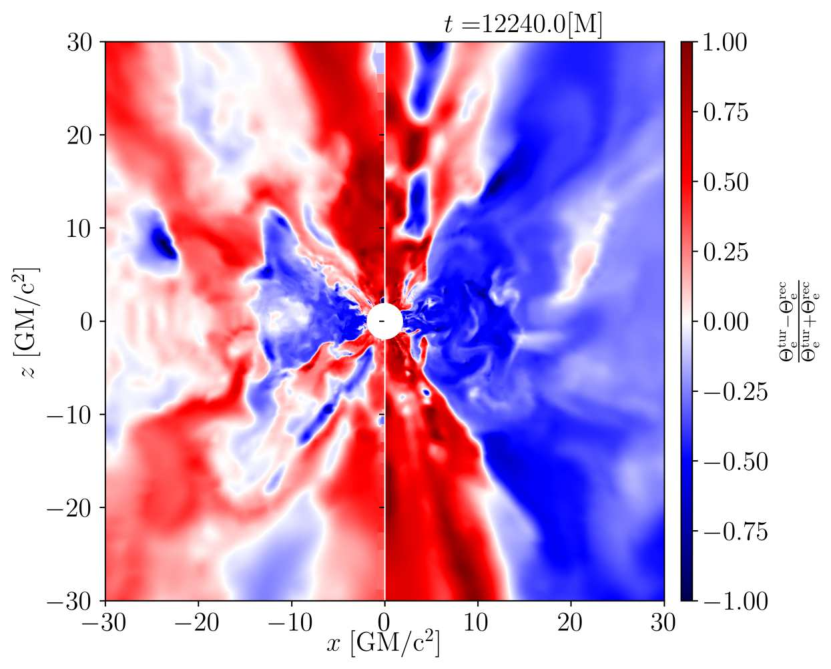
To compare turbulence and reconnection heating more directly, Figure 14 contrasts their electron temperatures cell by cell for M20a3D at . The left-right asymmetry simply reflects the azimuthal asymmetry of the underlying flux-rope-bearing accretion flow. The comparison shows that turbulence heating raises the temperature more strongly in the jet and sheath, whereas reconnection heating favors the dense disk. Since the two models have similar mass-accretion rates ( and ), this temperature difference is the main reason why the turbulence-heating case is much brighter at 138 THz than the reconnection-heating case (Figure 15). In the reconnection-heating model, even the hottest ropes remain cooler than their counterparts in the turbulence-heating run, despite the hotter torus.


Emission Region at NIR Frequencies
All models are normalized at 230 GHz through the accretion-rate calibration, so their mean NIR levels are free to differ. Figure 15 shows the resulting NIR light curves for M20a3D under the different heating prescriptions11 1 Because the reconnection-heating model is much fainter in the NIR, its light curve is multiplied by a factor of 20 in the figure.. In contrast to the 230 GHz case, the two-temperature models are now much more clearly separated from the parameterized prescriptions. The reconnection-heating curve is roughly an order of magnitude fainter than the other three, whereas the model with is the brightest. The turbulence-heating result remains closest to the model with . During the most flare-active intervals, – and –, the turbulence-heating light curve also develops sharper spikes than either model. The curve is brighter, but it is also much smoother. These differences show that the dominant NIR-emitting region depends very strongly on the heating prescription. Even the brightest modeled peaks remain one to two orders of magnitude below the observed Sgr A∗ NIR range of 5 to 25 mJy [4], which is expected because real NIR flares are thought to be dominated by non-thermal radiation. The comparison therefore reinforces the conclusion that a non-thermal component is needed to reproduce the observed flare amplitudes [338, 99, 316, 343], although that extension is left to future work.
Even so, the thermal NIR emission remains diagnostically useful. In every model, the NIR variability is governed mainly by the hottest plasma, with typical temperatures and peak values around . Figure 11 shows that, for fixed magnetic field, the thermal synchrotron emissivity continues to increase with electron temperature up to roughly , so the brightest NIR zones naturally coincide with the hottest gas. As already emphasized by [155], the prescription cannot reproduce the fine substructure of hot plasmoids and current sheets. The present 3D calculations lead to the same conclusion: the self-consistent two-temperature solutions retain much more small-scale structure than the parameterized model (Figure 9). Figure 16 identifies the dominant NIR-emitting zones by showing the emissivity distributions of the turbulence- and reconnection-heating models after averaging over and at . In the turbulence-heating run, the NIR emission is concentrated in the sheath. In the reconnection-heating case, the much weaker NIR component is centered instead on the torus. The -averaged maps in Figure 16(b) and (c) also show a bright spiral-like structure associated with the flux rope. Relative to reconnection heating, the turbulence-heating prescription produces a brighter and more extended high-emissivity region, which naturally yields a larger total NIR flux.
Because the flux ropes contribute so strongly in the NIR, they are plausible counterparts of the observed NIR flares [3]. Reconstructed 3D flare orbits also favor a low-inclination plane [175]. This differs from MAD-based flare models, where the emitting structure remains close to the equatorial plane and therefore corresponds to an inclination nearer [273, 91, 243]. In the present simulations, most flux ropes occupy the sheath, where the characteristic inclination is lower, around , and where the structures evolve rapidly with time. Their orbital timescale is about , and most survive for only about one orbit before dissipating. The implied flare duration is therefore also of order 10–100 M, as suggested by Figure 16. In the turbulence-heating model, repeated energy release from these zones drives the strongest light-curve variability because the ropes themselves dominate the radiation (Figure 16(b)). The variability pattern therefore maps directly onto the evolution of the hottest plasma.
4 Summary and Conclusions
I performed 3D two-temperature GRMHD simulations of magnetized accretion flows around a rotating black hole initialized with multiple magnetic loops. Two loop scales, and , were studied. For the electron thermodynamics, I compared turbulent heating, reconnection heating, and a parameterized prescription. The main results are summarized below.
- 1.
The initial loop scale controls both magnetic dissipation and MRI activity in the torus. Shorter loops dissipate more efficiently and weaken the MRI, whereas longer loops permit a partial transition from SANE toward MAD. This matches the earlier 2D trend [155], although the 3D transition remains incomplete because the field never becomes strong enough to choke the inflow entirely.
- 2.
While only the first loop is accreted, the flow behaves much like the single-loop solutions of [208]. In that stage, the 230 GHz light curves are nearly identical across all heating prescriptions, whether they come from the evolved two-temperature model or from the reconstruction. Once loops of opposite sign begin to arrive, reconnection strengthens and the flow becomes strongly turbulent.
- 3.
After the turbulence is fully developed, the light curves depend strongly on the heating prescription. The turbulence-heating model and the case are the most variable because they receive a larger fraction of their flux from the strongly varying sheath. The reconnection-heating model and the case are less variable because a larger share of their radiation comes from the calmer equatorial flow.
- 4.
The electron temperature regulates the thermal emissivity in a highly frequency-dependent fashion. At higher frequencies, the radiation is dominated by hot structures such as erupting flux ropes. Since those ropes combine enhanced density with elevated electron temperature, they are more variable than the equatorial flow and produce both the filamentary image morphology and the strong high-frequency variability, especially in the NIR. At lower frequencies such as 43 GHz, the filamentary pattern is much less prominent.
- 5.
Compared with reconnection heating, the turbulence-heating model produces a broader electron-temperature distribution. It heats the jet and flux ropes more strongly while leaving the disk cooler. The same qualitative behavior already appeared in the 2D calculations [155]. Although the large-scale temperature structure still resembles the result, the most important differences arise on smaller spatial scales.
Overall, the 3D multi-loop calculations show that such accretion flows can produce thermal synchrotron behavior that is relevant to the observed variability of Sgr A∗. The models do not settle into the cleanest MAD states, even though many present EHT interpretations favor MAD-like solutions for Sgr A∗ [74]. More generally, however, no currently available model family, whether SANE or MAD, matches the full set of EHT constraints while also reproducing the required variability. That tension motivates exploring multi-loop accretion as an alternative flare scenario. In these simulations, reconnection in the jet sheath emerges as a plausible driver of the flaring activity. Thermal radiation alone still fails to supply enough NIR flux, so the next step will be to add non-thermal emission from the flux ropes and measure its contribution directly. A further limitation is the present 3D resolution: tearing and plasmoid formation are not yet fully resolved, which likely biases the electron temperature low inside those structures. Higher-resolution calculations, together with additional diagnostics such as visibility-amplitude morphology and M-ring fitting, will be needed to test the multi-loop picture more rigorously for Sgr A∗.
I also find that flux ropes with comparatively ordered magnetic fields contribute an increasing fraction of the total flux at higher observing frequencies. Their polarized emission should therefore become progressively more important. Testing that expectation will require polarized GRRT calculations in future work.
Supplementary Appendix
3.A Electron-Temperature Profile

The two-temperature models imply a more complicated relation between and plasma beta than a simple fit can describe. Figure 17 therefore plots the time- and azimuthally averaged - relation for M80a3D and M20a3D. In the jet regions of both models, some points reach , showing that the electron temperature can dominate locally. At low beta the scatter is substantial, again indicating that the simple prescription misses part of the underlying physics there. In the weakly magnetized, high- regime, the two-temperature models move toward similar values in M20a3D (lower panel of Figure 17). Even so, near , the reconnection-heating model gives a larger ratio, corresponding to the bluish disk region in Figure 14. The same qualitative trend already appeared in the earlier 2D study [155].
Chapter 4 Magnetic-Reconnection Flares in Sgr A∗ Across Multiple Wavebands
A prior version of this article appeared in Jiang H.-X., Mizuno Y., Dihingia I. K., Yuan F., Lin X., Fromm C. M., Nathanail A., and Younsi Z., 2025, ApJ, 990, 81 [154].
1 Astrophysical Motivation for Sgr A∗ Flares
Sagittarius A∗, hereafter Sgr A∗, is the supermassive black hole at the Galactic center and the nearest object of its kind that can be studied in comparable detail. EHT measurements place it at a distance of about and imply a mass of roughly [71]. Its surrounding accretion flow forms a bright ring with an observed diameter of [71]. Because the source is so close, Sgr A∗ provides an unusually clean laboratory for strong-gravity accretion physics. It is usually interpreted within the radiatively inefficient accretion-flow framework introduced by [329].
The emission from Sgr A∗ is strongly time variable, which makes the source observationally challenging [70]. Most of the time the system remains in a quiescent state, but it intermittently produces flares from the X-ray band down to the radio, with flux increases that can approach an order of magnitude above the baseline level [4, 26, 130, 275, 213, 218]. With the angular resolution of GRAVITY [2], [134] detected orbital hot-spot motion during NIR flares near the last stable orbit of Sgr A∗. ALMA polarimetry further shows that the sub-millimeter flare component is strongly polarized [314]. Comparisons of NIR and radio light curves further suggest that the variability amplitude grows toward higher observing frequency [4, 285].
Multi-band observations offer some of the strongest clues to the flare origin. In most reported events, the X-ray and NIR flares are simultaneous [102, 103]. The accompanying sub-millimeter variability usually appears later [103, 342, 334]. The statistical study of [316] found a characteristic delay of roughly minutes between 230 GHz emission and the 138 THz NIR band, although some individual events show lags as long as hours. This is consistent with the earlier measurements of [337], who showed that the 43 GHz peak precedes the 22 GHz peak. Taken together, these results are commonly interpreted as signatures of expanding plasmoids [337, 99, 251].
Many different scenarios have been invoked to explain the flares of Sgr A∗, including shocks in jets [192, 105] and magnetic reconnection operating directly inside the accretion flow [330, 327, 92, 226, 225, 99, 242, 91, 240, 60, 313, 265, 264]. Reconnection is often considered the leading explanation for the observed hot-spot behavior, but neither the field geometry nor the exact flare site is known with confidence.
A common class of models places the dissipation inside a MAD flow during episodes when magnetic flux erupts from the inner disk [273, 91, 264, 243, 25, 308, 23]. After the accumulated flux saturates, plasma is expelled from the near-horizon region and forms a rotating spiral. Reconnection then proceeds at the interface between that strongly magnetized ejecta and the surrounding gas. Polarization calculations for such vertically expelled flux ropes can reproduce loops in the Stokes plane [221], one of the signatures observed during Sgr A∗ flares [314]. In that picture, however, the hot spot remains embedded in the broader accretion flow, so pronounced outward propagation is not automatically obtained.
An alternative picture moves the dissipation site into the coronal flow, where flux ropes can form and rise away from the hole. [327] argued that turbulence together with differential rotation can generate both reconnection and flux ropes even without an initially multi-loop field. Once such structures appear, magnetic-pressure forces can push them outward and connect the flare more directly to a plasmoid ejection. Later 3D simulations [348] supported that scenario by producing flux ropes even from single-loop initial conditions. [178] then identified a flux rope whose projected motion and super-Keplerian orbit are consistent with the GRAVITY measurements. The radiative behavior of those structures has since been investigated in several later studies [10, 177, 201, 178, 97].
High-resolution calculations also suggest that toroidal magnetic flux can be transformed into poloidal loops through the joint action of the MRI and a mean-field dynamo [182, 159, 132, 266]. That process can generate polarity reversals inside the torus and produce the familiar butterfly pattern [90, 195, 196, 146, 345]. In wind-fed models such as [257, 261], the toroidal flux is usually assumed to come from the stellar wind, but the wind itself may already carry mixed polarities. If so, the torus could inherit a multi-loop magnetic geometry even in the wind-fed case, which remains only weakly explored. Motivated by that possibility, several studies have examined multi-loop field configurations with radial polarity reversals. When flux of alternating sign is swallowed by the hole, the system cannot maintain a large net magnetic flux efficiently, so the flow remains in the Standard And Normal Evolution (SANE) regime. Jet production is then weakened, while magnetic energy is dissipated preferentially through reconnection [155, 226, 225, 236, 333, 332, 188]. Large polarity reversals can also strongly affect jet stability and may arise from toroidal flux generated out of the original poloidal field [237, 150]. In addition, such inversions can repeatedly trigger reconnection and thereby accelerate non-thermal electrons [27, 242, 143, 28]. The multi-loop SANE picture therefore remains a plausible alternative to the better-known MAD flux-eruption scenario for Sgr A∗.
In our previous work [155, Jiang2024], we showed that multi-loop magnetic fields inside the torus generate many plasmoid chains through polarity inversions. In that study, the NIR emission was computed by GRRT post-processing with a purely thermal electron distribution inferred from the GRMHD data. That setup produced NIR emission that was too weak to match the observed flares of Sgr A∗. Here I extend the analysis by including both thermal and non-thermal electrons when modeling the radiative output of polarity-inversion events. With that addition, the same magnetic configuration can produce strong NIR flares compatible with the observations and can also generate natural time delays between different bands.
The rest of this chapter is organized as follows. Section 5.2 describes the GRMHD model together with the GRRT post-processing setup, Section 5.3 presents the results, and Section 5.4 summarizes the conclusions.
2 Simulation Model and Radiation Setup
1 GRMHD and GRRT Setup
To connect directly with the earlier study, I adopt a setup closely related to the 3D GRMHD model of [Jiang2024]. Very short loops dissipate magnetic energy too quickly, whereas very long loops launch jets that are too strong, so the present calculation uses an alternating-polarity multi-loop field with an intermediate wavelength following [226]:
| (1) | ||||
The parameter sets the radial scale of the magnetic loops. In the present model I adopt , where is the gravitational radius. The normalization of is chosen so that the minimum plasma beta is , with . The initial gas distribution is a Fishbone-Moncrief hydrostatic torus [113]. I set , , and fix the black-hole spin to . Further details of the GRMHD setup and numerical resolution are collected in Appendix 1 and 2. The electron temperature is evolved with the two-temperature method of [255]; the specific prescription used here is summarized in Sec. 2.
To compute the observables, the GRMHD snapshots are post-processed with the GRRT code BHOSS [325, 326]. Transfer coefficients are evaluated following [194]. Non-thermal radiation is modeled with a eDF restricted to . The local value of is assigned through a sub-grid prescription calibrated against turbulent plasma simulations (see Sec. 2). Whenever the fit falls outside the allowed interval, which can happen for or for very weak magnetization , the non-thermal synchrotron emissivity is set to zero (Appendix 5). The thermal emissivity is removed only in strongly magnetized regions with . Accordingly, the total emissivity is written as , where measures the fraction of the local energy budget associated with magnetic energy; its full definition is given in Sec. 2 and in [123]. At high frequencies, the cooling correction proposed by [273] is also applied; the implementation is summarized in Appendix 3. Throughout this chapter, Sgr A∗ is modeled with mass and distance [5]. The ray-traced images cover a field of view of , equivalent to , on a grid. The inclination relative to the spin axis is fixed at . The GRMHD mass unit is normalized by requiring a flux of at 230 GHz. With that choice, the model approximately reproduces the observed SED from millimeter to NIR frequencies (Appendix 1). The GRRT analysis uses snapshots between 8,000 and , when polarity reversals are most frequent and the NIR activity is strongest.
2 Thermal and Nonthermal Turbulence/Reconnection Models
We compute the electron temperature by evolving the electron entropy while including sub-grid heating from both turbulence and magnetic reconnection [160, 268]; a broader review of these ideas is provided by [96].
The NIR flares of Sgr A∗ are unlikely to be reproduced with a purely thermal model alone [273, 329]. We therefore supplement the thermal component with sub-grid non-thermal prescriptions calibrated by Particle-In-Cell simulations of turbulence and reconnection. The synchrotron emissivity is evaluated with a kappa eDF, which connects a Maxwell-Jüttner-like core smoothly to a power-law tail [123, 318, 89]. In the high-energy tail, one may roughly identify , so acts as an effective spectral slope. The local value therefore stands in for unresolved plasma microphysics. In this chapter, we use a sub-grid prescription based on PIC turbulence studies [202].
The eDF is written explicitly as
| (2) |
where is the electron number density, is the electron Lorentz factor, measures the width of the distribution, and is a normalization constant (see [234] for details). The role of is analogous to the power-law index in a standard power-law eDF. When , the eDF approaches the Maxwell-Jüttner form (see Figure 4 of [123]). The width parameter controls the energy spread [123]; in the limit , it reduces to the dimensionless electron temperature . We then evaluate the non-thermal synchrotron emissivity using the fitting formulae of [194].
For , we adopt two fitting expressions motivated by PIC calculations, one for special-relativistic turbulence [202, ] and one for magnetic reconnection [27, ]. They are written as
| (3) |
| (4) |
Here, denotes the magnetization and is the plasma-beta parameter.
Following [89, 86], we use the non-thermal acceleration efficiency to determine the width of the kappa distribution. In [89], the corresponding expression is
| (5) |
The first term describes the thermal contribution, and the second encodes the non-thermal one; and are the proton and electron masses. We assume that the non-thermal population draws its energy from the magnetic reservoir. Because the fitting formula for the emissivity of a kappa eDF is valid only for [194], we enforce that interval in both prescriptions. The parameter quantifies how much of the magnetic energy is used to broaden the kappa distribution [123], namely the magnetic-energy fraction within the total energy budget. Earlier studies often fixed to constant values such as 0, 0.5, or 1.0 [82, 123]. In a realistic flow, however, the non-thermal acceleration efficiency should depend on the local plasma conditions. The turbulence-based and reconnection-based fits used here are taken from [202] and [27]:
| (6) |
| (7) |
Accordingly, we use in Eq. 5 to set the local weight of the non-thermal electron population.
Following [123], we express the total emissivity and absorptivity as the sum of thermal and kappa-based terms:
| (8) | ||||
The same efficiency factor from Eqs. 6 and 7 is used here. In practice, we first form the combined emissivity and absorptivity and then provide those total coefficients to the GRRT solver.
In weakly magnetized gas with , we retain only the thermal emissivity and absorptivity. The hybrid prescription of Eq. 8 is used only above that threshold.
The sub-grid prescriptions are activated through thresholds tied to the large-scale plasma state. Non-thermal particles are added only where the resolved fluid variables indicate conditions favorable for reconnection, because the global simulation cannot resolve the current sheets and other microphysical structures in which the acceleration physically takes place. In that sense, the method transfers the results of earlier small-scale studies into the global calculation, while a fully self-consistent cross-scale treatment remains beyond the resolution of the present model.
3 Results and Physical Interpretation
1 Multi-Frequency Light Curves
Earlier work has shown that multi-loop accretion flows can undergo repeated reconnection as successive polarity inversions pass through the system [226, 242]. Those inversions create many current sheets and plasmoid-rich structures and therefore offer a natural route to the kind of flare activity observed in Sgr A∗ [4]. In such regions, electrons may be accelerated into a non-thermal tail, allowing magnetic energy to be transferred into the eDF and to power bright NIR events.
After adding non-thermal electrons in the GRRT post-processing, I compute light curves at multiple frequencies over the interval 8,000–, when polarity inversions occur most often; the result is shown in Figure 1. Panels (a)–(d) display the emission at 22 GHz, 43 GHz, 86 GHz, and 138 THz (NIR) in black, red, blue, and purple. The 138 THz curve shows three major flares near , 9000, and . Their peaks reach about 14 mJy, whereas the minima fall below 0.1 mJy. In that sense, the modeled 138 THz variability is broadly consistent with the observed NIR behavior of Sgr A∗ [4].
Panels (a)–(d) of Figure 1 also reveal a clear frequency-dependent lag between the NIR and the millimeter-radio bands. As in earlier studies [316, 25], I quantify that lag with the cross-correlation function (CCF); the implementation is summarized in Appendix 3 and Sec. 6. Panel (e) shows the corresponding DCCFs for 22 GHz, 43 GHz, 86 GHz, and 138 THz, with shaded bands indicating the uncertainty in each lag bin. The inferred delays are about 16.5 minutes between 22 and 43 GHz, 20.2 minutes between 43 and 86 GHz, and 34.8 minutes between 86 GHz and 138 THz. The lag therefore becomes larger toward lower observing frequency. The flare near illustrates this particularly clearly, with the radio peak following the higher-frequency NIR event. That ordering matches the observational picture in which lower-frequency flares lag behind higher-frequency ones [337, 336].


2 Physical Origin of the NIR Flares
In the multi-loop GRMHD models, polarity inversions are accompanied by comparatively ordered magnetic fields, enhanced density, and elevated electron temperature in the jet sheath. These properties make them natural candidates for the flare-producing regions in Sgr A∗ [226, 236].
Figure 1(d) shows that the modeled NIR light curve reaches flare peaks nearly two orders of magnitude above the quiescent level. The amplitude, duration, and peak brightness remain close to the values reported by [4]. To identify the emitting region, I examine the 134 THz emissivity in 3D volume renderings with magnetic-field lines, together with the corresponding NIR GRRT images, for a flaring state (, total flux 4 mJy) and a quiescent state (, total flux 0.6 mJy) shown in Figure 2. Panels (a) and (b) show that the flaring snapshot contains an extended spiral emissivity feature inside the accretion flow. In the enlarged upper-left region of panel (a), this bright structure coincides with strongly twisted magnetic field lines. The two sides of the spiral have opposite polarity, identifying the feature as a polarity-inversion layer. The bright emission is therefore linked directly to magnetic-energy release in a large-scale polarity inversion. By contrast, the quiescent state shows neither the strongly twisted field geometry nor the extended spiral emissivity pattern, either in the 3D rendering or in the GRRT image. Small polarity reversals are still present, but they contribute little radiation.
Panel (c) contains an extended bright feature, shown in reddish colors, that is absent from the quiescent image. To determine where this radiation originates, I track how the intensity accumulates along individual geodesics through the GRMHD domain. During the GRRT post-processing, both the ray trajectory and the local intensity are recorded, as described in Appendix 2. This makes it possible to identify the part of the flow where each photon packet acquires most of its flux while crossing the polarity inversion. In panel (c), two representative points inside the brightest region are marked by a gold triangle (Position A) and a blue star (Position B). Figure 9 then shows where the corresponding rays accumulate most of their intensity. Once the rays have left the flaring zone, their intensity changes only weakly before reaching the observer. For Position A, the dominant contribution comes from approximately , , and , whereas Position B is dominated by emission from about , , and . In the 3D rendering of panel (a), those two locations are marked by the same gold and blue spheres and coincide with distinct emissivity peaks. As these structures rotate toward the observer, whose azimuth is zero, Doppler boosting amplifies their radiation and produces the flare. The blue sphere lies directly on the reconnection site and corresponds to strong NIR emission in the GRRT image. This mapping shows that the brightest NIR features are generated by polarity-inversion events.
As Figure 2(a) illustrates, large-scale polarity inversions generate filamentary emissivity structures. To characterize the local plasma there, I extract the one-dimensional profile across the current sheet shown in Figure 3. That cut provides direct evidence for magnetic reconnection.
Figure 3(a) shows that the dominant toroidal component () reverses sign completely, identifying it as the main magnetic-energy reservoir dissipated in the event. By contrast, the poloidal component () keeps the same sign and therefore acts only as a weak guide field. This agrees with the global result that the ratio of reconnecting to guide field remains well below 0.1, indicating weak-guide-field reconnection. Figure 3(b) further shows that the upstream plasma in the reconnection layer has and . These plasma conditions fall exactly in the regime where the adopted sub-grid models predict efficient non-thermal acceleration. The full 3D distributions of and are shown in Figure 4(a) and (b). In the GRRT calculation, the non-thermal acceleration efficiency varies across the domain and is plotted in Figure 4(c); it injects non-thermal electrons directly into these localized structures. The resulting non-thermal radiation is therefore concentrated at the polarity inversions and contributes directly to the observed NIR flares. Figure 4(d) shows that most of the volume remains close to thermal (), whereas the polarity-inversion layer reaches low , indicating the strong non-thermal component responsible for the enhanced emission.
3 Energetic Requirements for the NIR Synchrotron Flares
In this section, I show that the magnetic-reconnection regions identified in the GRMHD simulation contain enough energy to accelerate electrons to the energies required for the NIR flares. The synchrotron frequency characteristic of an electron with Lorentz factor radiating in a magnetic field is
| (9) |
To estimate the electron energy needed for NIR emission, we adopt a representative flare wavelength of , corresponding to an observed frequency of Hz. In the reconnection zones of our simulation, the magnetic field is typically . Solving for the Lorentz factor then gives
| (10) |
This estimate shows that the observed NIR radiation requires highly relativistic electrons, with Lorentz factors of order .
It is important to distinguish the ion-dominated bulk-flow magnetization from the electron magnetization , because the latter is the quantity more directly tied to particle acceleration. In the GRMHD simulation, the measured magnetization refers to the bulk fluid, whose inertia is dominated by protons. The value measured in the reconnection sites therefore corresponds to the ion magnetization ():
| (11) |
Direct magnetic energization of electrons, however, is governed by the electron magnetization , defined using the electron rest-mass energy density:
| (12) |
For a quasi-neutral electron-ion plasma with , the two magnetizations differ only by the proton-to-electron mass ratio:
| (13) |
Using the simulated value , we estimate the corresponding electron magnetization in the reconnection region as
| (14) |
The resulting local electron magnetization is therefore , which measures the magnetic energy available per electron. That scale is comparable to the kinetic energy needed for the emitting particles, . In other words, the relation is satisfied. This supports the conclusion that the magnetic-reconnection events present in the GRMHD simulation can accelerate electrons to the Lorentz factors required by the observed NIR flare. Additional processes, such as stochastic acceleration within a turbulent reconnection layer, will likely modify the final particle distribution, but this basic energy-budget estimate already supports the physical plausibility of the proposed mechanism.
4 Time Delays and Radio-Band Flares
One well-known property of Sgr A∗ flares is that the radio peaks usually occur after the NIR and X-ray peaks [316]. Earlier interpretations associated that delay with adiabatically expanding hot spots [337, 178, 204], although the physical nature of those transient structures remained uncertain. The previous subsection showed that, in the present model, the NIR flares are produced by polarity-inversion events and that the millimeter flares appear later.
At millimeter wavelengths, plasma self-absorption becomes important. A polarity inversion therefore produces an evolving emitting structure whose visibility depends on the local opacity. To determine the origin of the lag, I examine the 43 and 86 GHz flares at and , which follow the NIR event discussed in Sec. 2. Panels (a) and (b) show the corresponding GRRT images, while panels (c) and (d) trace the intensity accumulated along the geodesic that passes through the brightest pixel, marked by a red cross. Although the projected peaks are nearly coincident at the two frequencies ( at 86 GHz and at 43 GHz), the radiation originates from slightly different parts of the flow. Panels (c) and (d) show that the emitting geometry changes with frequency. At both 43 and 86 GHz, most of the radiation still comes from the same compact region inside . Even so, the dominant 43 GHz contribution is displaced slightly outward and toward higher latitude relative to the 86 GHz emission site. That outward shift is the most plausible source of the lag. Radiative-transfer effects reinforce the trend, because the lower-frequency photosphere lies farther out in denser and more opaque plasma. Observationally, a modest delay of about 20 minutes has also been reported between 230 GHz and NIR flares [316]. In general, however, theory does not predict a large lag there because the plasma should already be mostly optically thin at those frequencies. When such a lag is observed, it may therefore indicate additional structure either in the flare mechanism itself or in the emitting region [Jiang2024].
Once this outward shift of the millimeter emitting region is recognized, the connection between the NIR and millimeter flares becomes straightforward. The millimeter events occur after the NIR flare but follow the same broad temporal evolution, which strongly suggests a common physical origin. Because self-absorption matters at millimeter wavelengths, Figure 6 compares light curves computed with and without it. When self-absorption is removed, all radio bands peak simultaneously with the NIR flare, directly tying them to the same underlying event, namely the polarity inversion shown in Figure 2. The lags appear only after self-absorption is restored, because the lower-frequency radiation remains hidden until the polarity-inversion structure has moved outward into gas that is less dense and less opaque. The delayed radio peaks therefore arise naturally, while the shared origin of the NIR and millimeter flares remains unchanged. Taken together, these results show that a single polarity-inversion event can generate both the NIR and radio flares, with the observed delays set by the combined effects of evolving geometry and frequency-dependent self-absorption.
4 Summary and Implications
I carried out 3D two-temperature GRMHD simulations of magnetized accretion flows around a rotating black hole threaded by multiple magnetic loops and combined them with GRRT calculations that use hybrid thermal and non-thermal electron distributions. The analysis focused on the origin of the multi-band flares in Sgr A∗ and on the delays between those bands. The main conclusions are:
- 1.
Non-thermal electrons are necessary to reproduce the observed NIR light curves of Sgr A∗. In a SANE flow with a multi-loop magnetic topology, large-scale polarity inversions can produce NIR flares whose amplitudes and variability are comparable to the observations.
- 2.
Filamentary structures appear in the GRRT images during the NIR flares. By tracking both the ray paths and the accumulated intensity along them, I show that the brightest parts of the image originate in large-scale polarity inversions close to the black hole.
- 3.
The GRRT light curves show clear multi-frequency delays. The millimeter-radio flares reach maximum after the NIR flares, and the lag can be as large as roughly 50 minutes, well within the observationally reported range.
- 4.
The radio flares are produced by the same large-scale polarity-inversion events that generate the NIR flares. Their delayed appearance is caused by frequency-dependent self-absorption at millimeter wavelengths: the emitting structure must move outward before the lower-frequency radiation becomes visible.
The results support a picture in which large-scale polarity inversions in SANE accretion flows can account for the NIR flares of Sgr A∗ while remaining broadly consistent with the current data. In that sense, the scenario provides a credible alternative to the MAD-based flare models that are more often discussed for Sgr A∗ [273, 91, 243, 221, 25]. It also reproduces several additional observational traits of the Galactic center. In particular, the models do not produce a persistent relativistic jet (see Appendix 4 for a fuller discussion of the accretion state and jet behavior), they naturally generate delays between the NIR and 43 GHz flares, and they provide a reasonable match to the observed SED.
The multi-loop configuration still has clear limitations. It does not maintain frequent, long-lived, large-scale polarity inversions, and earlier work suggests that it more closely resembles a transitional state [155, 151]. Understanding how Sgr A∗ sustains persistent flaring therefore remains an open problem. Although the adopted resolution is high enough to capture the formation and large-scale evolution of magnetic polarity inversions, it is not sufficient to resolve the smallest turbulent structures or the asymptotic plasmoid-dominated reconnection regime fully. Ultra-high-resolution GRMHD calculations with GPU-accelerated codes [264] can reach a regime in which reconnection becomes nearly grid independent, but such simulations require far more computational resources than are available here. The present global 3D study therefore concentrates on the large-scale polarity-inversion process rather than on the detailed microphysics of the reconnection layer.
Because the resolution remains limited, the disk dynamo is not fully resolved and therefore does not continuously regenerate alternating polarities [90, 195, 196]. I also do not resolve the tearing instability needed for plasmoid formation at the reconnection site [155, 264], which may reduce the number of non-thermal electrons. In addition, a polarity inversion becomes an observable flare only if two conditions are satisfied: the event must be intrinsically energetic enough, and the emitting plasma must move toward the observer rapidly enough for Doppler boosting to amplify the signal. Equally energetic events moving away from the line of sight would instead be de-boosted and appear faint. These geometric selection effects therefore shape both the apparent flare rate and the measured flare amplitude.
The present GRRT calculation also neglects Compton scattering, so the model cannot yet address the X-ray counterparts. Synchrotron self-Compton emission may contribute significantly to the observed X-ray flares [104, 95], but that channel is not included here. In addition, the current ray-tracing method is limited when one tries to extract truly local properties of the flaring region; a Monte Carlo treatment that follows photons from a reconnection event to infinity would improve this aspect. These missing ingredients will be explored in future higher-resolution simulations that can also address the weaker X-ray flares.
Supplementary Appendix
4.A Code Configuration
1 GRMHD Setup with KHARMA
All simulations in this appendix are evolved with KHARMA11 1 https://github.com/AFD-Illinois/kharma [247], the GPU-oriented GRMHD code built on top of iharm3D [248]. Numerically, both codes descend from the conservative ideal-GRMHD scheme introduced in HARM [126]. In the Eulerian form used here, the governing equations are
| (15) | ||||
Here is the rest-mass density, is the fluid four-velocity, are the connection coefficients, and are the three- and four-magnetic-field components, is the stress-energy tensor, and is the metric determinant [126]. On the implementation side, KHARMA combines the Parthenon mesh infrastructure [135] with the Kokkos performance-portability layer [295]. Numerical floors are applied to stabilize the evolution in low-density, highly magnetized regions, especially near the horizon and along the rotation axis [Rezzolla-Zanotti2013]. Concretely, I set and , and cap the magnetization and Lorentz factor at and . Magnetic-flux conservation is maintained with Face-Centered Constrained Transport (Face-CT) [247]; more specifically, I adopt the three-dimensional gs05c variant based on the upwind method of [128] as generalized by [129].


2 Resolution and Initial Magnetic Geometry
The mesh starts from zones and is supplemented by two static-refinement levels, so the finest effective resolution becomes . Refinement is applied only inside a selected region of Wide-pole Kerr-Schild (WKS) coordinates; see [65] together with [199, 197, 256] for related coordinate choices. Radially, that high-resolution region extends from to , while in polar angle it covers to . Figure 7 marks this refined domain in red.
The magnetic seed field shown in the right panel of Figure 7 is a radial multi-loop configuration in which neighboring loops reverse polarity from one ring to the next.
3 Cooling Model
Radiative cooling can reshape the particle distribution by limiting the highest Lorentz factor and altering the effective power-law slope. Here I adopt the simple approximation introduced by [273]:
The synchrotron cooling timescale is
| (16) |
where is the Thomson cross-section, is the magnetic energy density, is the Lorentz factor, and . The photon escape time is approximated by the light-crossing time . Cooling therefore becomes important near
| (17) |
which corresponds to a characteristic break frequency of
| (18) |
This corresponds to strong cooling above approximately Hz. In practice, following [273], I divide the emissivity and absorptivity from Eq. 8 by whenever . Including this prescription suppresses the X-ray flux substantially and produces a more realistic high-frequency SED.
4.B Supplementary Material
1 Spectral Energy Distribution

Figure 8 places the simulated spectral energy distributions beside the available multi-wavelength measurements. The millimeter and sub-millimeter fluxes come from [346, 21, 44, 46, 43], while the infrared points are taken from the compilation of [81], which is itself based on [124, 125].
The calculation uses two alternative prescriptions for the electron thermodynamics and non-thermal component (see Sec. 2). One is tied to turbulent dissipation and the other to magnetic reconnection. Because the simulation does not resolve every eddy and current sheet, it is not yet possible to assign those microphysical channels to each fluid element in a fully self-consistent way. Instead, I follow the pragmatic strategy used in earlier flare studies [123, 321] and examine the observational consequences of the two prescriptions separately.
The comparison in Figure 8 shows that the two models remain almost indistinguishable through the millimeter band, where thermal synchrotron emission from the bulk flow dominates. Their predictions begin to separate only toward the infrared and above, once the non-thermal electrons become important. In that regime, the turbulence-based prescription more often falls inside the observed infrared range and can generate NIR peaks of roughly 10–25 mJy, comparable to the flares reported by [134]. For that reason, I keep the turbulence-based model as the fiducial choice in the main discussion.
The low-frequency radio emission below 43 GHz is still underestimated. In GRMHD jet solutions, adiabatic expansion cools the outflow and lowers the electron temperature, whereas the observed flat radio spectrum points to a jet that stays closer to isothermal. The multi-loop initial field used here also weakens the large-scale jet because repeated polarity reversals impede the buildup of a persistent outflow, which further worsens the radio deficit.
2 Ray Paths and Intensity in the GRRT Calculation


To determine where each image pixel acquires its flux in the GRRT calculation, I extract both the null geodesic and the accumulated intensity along that path. Figure 9 displays this intensity history in spherical coordinates, making it possible to identify the region from which most of the radiation is received and therefore to localize the flare site.
The yellow and blue curves correspond to the two rays passing through Positions A and B in panel (c) of Figure 2. The shaded interval marks the part of the trajectory where the intensity increases most strongly, which identifies the coordinates of the dominant emitting region. The same site can then be located directly in the 3D volume-rendered view shown in Figure 2.
Panel (d) of Figure 9 gives the same two trajectories in full three dimensions.
3 Discrete Cross-Correlation Function
The cross-correlation function (CCF) is a standard tool for measuring the time lag between two time-dependent signals [19]. In practice, one usually uses the discrete cross-correlation function (DCCF) rather than the continuous CCF. For two light curves and , the lag between a pair of points and is
| (19) |
After defining the lag sequence , all pairs whose separations satisfy are grouped together, and each pair is assigned the correlation coefficient
| (20) |
where and are the averaged values of the two light curves, and and are their standard deviations. Thus, the DCCF within the given bin of time lag is obtained as
| (21) |
Here is the number of point pairs that fall inside the lag bin . I estimate the DCCF uncertainty from the standard deviation within that bin:
| (22) |
4 Accretion Stages in the Multi-Loop Model and Convergence Check

Figure 10 summarizes the evolution of the magnetic flux, jet power, and accretion rate. In panels (a)–(c), I use the horizon-based definitions of and from [244] together with the jet-power definition of [226]. Specifically, and are measured at the event horizon, while the jet power is computed at as , with spanning the funnel region defined by . The joint evolution of and indicates that the system passes through distinct accretion stages. The simulation is followed beyond . After about , the inner flow inside roughly reaches a quasi-steady state. Before , repeated polarity reversals drive stronger fluctuations in both and , and those same inversions generate the NIR flares shown in panel (d). At later times, the available magnetic energy declines, the inversions cease, and the NIR variability relaxes back toward a quiescent level. Because frequent reconnection during the inversion phase suppresses jet formation, the jet power in panel (b) stays close to zero for most of the run and no sustained jet develops.
Panels (a)–(c) also compare the SMR run with a run without refinement, using resolutions of and , respectively. The close agreement in their time histories indicates that the simulation is numerically well converged at the level relevant for this analysis.
5 Effect of

In the GRRT post-processing, highly magnetized cells are excluded through the cutoff parameter , so the NIR light curves can depend on that choice. Here I test the sensitivity by comparing the fiducial value with two alternatives, and , as shown in Figure 11.
The main effect appears at the low-cutoff end: using noticeably suppresses the light curve. Raising the cutoff to , by contrast, produces a result that is almost identical to the fiducial case. This indicates that is already large enough for the present application and that increasing it further has little practical effect on the GRRT output.


6 Additional Statistical Analysis of the Light Curves
This subsection examines the light curves with several additional statistical diagnostics in order to isolate their characteristic timescales and variability patterns.
The multi-frequency light curves in Figure 1 already suggest that different bands are governed by different parts of the flow. That contrast becomes clearer in Figure 12. In panel (a), the autocorrelation function (ACF; see [45, 304] for the definition) drops rapidly at 138 THz, indicating short-timescale variability. The radio bands (22–86 GHz), by contrast, retain correlation over much longer lags and therefore appear more periodic. Panel (b) shows that the burstiness coefficient [157] increases with frequency, implying that the high-frequency emission is more clustered in time and more stochastic. Panel (c) shows the memory coefficient [157]. It is weakly positive at 22 GHz, becomes negative at intermediate frequencies, and then shifts back toward less negative values at 138 THz. Taken together, these trends point to shorter-lived events with smaller separations at high frequency, where compact turbulent regions dominate, while the lower-frequency variability is produced by larger and more slowly evolving structures.
Panel (d) of Figure 12 expresses the same contrast in the wavelet domain. The three radio-band spectra nearly coincide, indicating a common variability pattern with a dominant timescale near . The 138 THz curve is different: most of its power is concentrated near , and a weaker component remains around . This suggests that the NIR outbursts are either shorter in duration or more closely spaced in time, most likely because they originate from rapidly orbiting gas in the inner 3– at roughly (see panel (a) of Figure 2). In other words, the high-frequency end of the spectrum encodes the narrow spike-like structures seen in the NIR flare light curves.
Chapter 5 Tilted MAD retrograde precession
Retrograde Precession from Magnetic Torques in Tilted Black-Hole Accretion Flows
A shorter version of this work was published in ApJ, volume 995, article 112 (2025), by Jiang H.-X., Mizuno Y., Lai D., Dihingia I. K., and Fromm C. M. [156].
1 Physical Motivation and Context
Spin-misaligned accretion should arise in many black-hole systems of interest, from X-ray binaries to active galactic nuclei [106, 340, 133, 282, 166]. Whenever the angular momentum of the supplied gas differs from that of the hole, the inner flow settles into a tilted disk-jet configuration rather than an aligned one [119, 246]. Frame dragging then induces Lense-Thirring precession and continuously redistributes angular momentum throughout the tilted flow [292, 223].
How often such tilts occur depends on both how the system formed and how it is fed later on [262, 32]. Gas captured from winds, disrupted stars, or post-merger inflows need not share the spin axis of the central hole, so warped and tilted disks are expected to be common [115, 116, 180, 179, 62]. This picture has been invoked for microquasars such as SS 433, GRO J1655-40, and GRS 1758-258 [191, 215, 187, 280], and it is likewise relevant to tidal-disruption events and post-merger AGN, where the impact geometry is often effectively random [339, 289, 120, 238, 284, 22, 165, 52, 51]. Thin disks can diffuse into Bardeen-Petterson alignment [274, 30, 181, 179], whereas thick disks communicate warps as bending waves and may preserve a global LT mode in the SANE regime [115, 116, 117, 180, 312, 339]. That coherence requires the sound-crossing time to remain shorter than the precession time [118]; once MRI-driven spreading enlarges the torus, the precession frequency tends to drop [180].
The MAD state introduces another torque channel. When large-scale magnetic flux accumulates near the horizon, the jet and ordered field can torque the disk toward the black-hole equator and compete directly with LT precession [62, 198, 241, 254]. That makes the persistence of precession uncertain in strongly magnetized systems. Indeed, [62] found no compelling long-lived precession in very extended tilted MAD tori [198, 62]. The question is particularly relevant for M 87∗, whose accretion flow is widely interpreted as MAD [75, 331] even though VLBI observations suggest jet precession [83]. In this chapter I examine whether tilted MAD disks can continue to precess across several magnetic setups. The central result is that once the accumulated flux becomes strong enough, the magnetic torque can flip the sign of the net precession rate and drive retrograde motion of both the disk and the jet.
Section 6.2 presents the simulation results, Section 6.3 summarizes the main conclusions, and the Appendix collects the numerical setup and related supplementary material.
2 Results


This section analyzes a suite of tilted-disk GR(M)HD calculations carried out with KHARMA, the GPU implementation that succeeds iharm3D [248]. By varying both the magnetic-field configuration and the hole spin , the model set isolates the competition between LT frame dragging and magnetically induced torques. Details of the numerical setup and grid choices are deferred to Appendix 6.A and 6.B.
1 Precession and Tilt in the GRMHD Simulations


Figure 1 shows the evolution of the disk precession angle and tilt angle for four representative runs. The angle definitions follow [180] and are summarized in the Appendix11 1 The tilt angle is the angle between the disk angular-momentum vector and the positive -axis, while the precession angle is the position angle of that vector. Following [180], the jet orientation is measured by isolating the magnetically dominated jet and applying the same construction..
The hydrodynamic control (black) and the two SANE models (yellow and green) all exhibit ordinary prograde LT precession, meaning that the disk turns in the same sense as the black-hole spin. In T25a094HD, the precession remains comparatively steady because the torus expands only modestly. The two SANE cases, T25a094wSANE and T25a094sSANE, differ only in field strength and therefore provide a clean magnetic comparison. The weaker-field run stays close to the hydrodynamic behavior, showing that magnetic stresses remain secondary there. The stronger SANE case, by contrast, aligns more rapidly and precesses more slowly, consistent with stronger magneto-spin coupling. In both SANE runs the precession signal fades substantially at late times ( and ).
In the MAD case the behavior changes qualitatively. Once the horizon-threading flux reaches the usual MAD level ( for prograde holes; [291]), the blue curve in Figure 1(a) crosses through zero and becomes retrograde. Early in the evolution, before the jet is established, model T25a094nMAD still resembles the hydrodynamic reference and follows LT-driven prograde motion. After strong magnetic flux piles up and the jet forms, the sign flips and the disk precesses opposite to the hole spin. The simplest interpretation is that the magnetic torque has overtaken the LT torque. The same change of sense is visible in the 3D renderings of Figure 2: between the two snapshots the tilted jet-disk system clearly rotates opposite to . At the same time, the tilt declines in every magnetized run because magneto-spin alignment steadily draws the flow closer to the spin axis [198, 62]. A gradual tilt decay is also present in the HD model because the initial tilted torus is not an exact equilibrium.
The jet broadly mirrors the disk orientation, but its response is noisier. In Figures 3(a) and (b), the red curves show that the jet reacts more sharply than the disk to the flux eruptions characteristic of the MAD state. That behavior is expected because the jet is threaded by a more coherent large-scale field than the dense disk body, so magneto-spin alignment acts on it more efficiently and reduces the jet tilt faster.
The transition in T25a094nMAD therefore marks the point where magnetic forcing overtakes LT forcing. The strongly magnetized SANE case supports the same picture in a weaker form: its slower precession rate cannot be explained by disk expansion alone and already points to a magnetic reduction of the ordinary LT signal.
The radial behavior makes the competition clearer. Since , LT forcing is concentrated toward the inner flow. Figures 3(c) and (d) show radial profiles of the disk precession and tilt in T25a094nMAD, obtained by dividing the flow into annuli eight cells wide and integrating the angular momentum in each shell separately. Near the hole, at , frame dragging twists the disk toward positive . As time passes, however, the contrast between inner and outer radii diminishes, so the profile gradually smooths even after the global precession has almost stalled by . The tilt profile shows a similar trend: the inner disk aligns first, again consistent with strong magnetic alignment. The end result is a significantly warped and twisted disk shaped jointly by LT precession, magnetic torques, and spin alignment, as illustrated by Figure 4(a).
2 Origin of the Magnetic Torque
A key question is how the field manages to reverse the precession sense even though the initial tilt is only moderate and the disk and spin axes are already fairly close. Figure 4 provides the essential clue. It compares the time-averaged density and poloidal field structure in the rotating model T25a094nMAD with the otherwise identical non-rotating control T25a0nMAD, averaged over –. When the hole does not rotate, the poloidal field stays roughly radial. When , however, the rotating spacetime drags the initially tilted field toward the spin axis, strengthens the toroidal component, and reorganizes the global magnetic geometry. The field therefore aligns faster than the dense disk body does, leaving a finite offset between the magnetic symmetry axis and the disk angular momentum for an extended period.
[170] proposed a simple model in which a misaligned disk threaded by a vertical magnetic field aligned with the black-hole spin axis experiences a magnetic torque that drives retrograde precession. Such a torque exists whenever a conducting disk is embedded in an inclined external magnetic field (see [169]). When the external field is misaligned with the disk axis , it projects a radial component onto the disk plane, , where is the angle between and and is the azimuthal angle around the disk. Meanwhile, the component perpendicular to the disk, for small , induces an azimuthal screening surface current , where and is the induced radial field on the upper disk surface. The interaction between and then produces a -dependent vertical force, which yields the magnetic torque per unit area [170]
| (1) |
This torque in turn produces a local retrograde precession,
| (2) |
where is the disk surface density and is the disk angular frequency. Comparing this with the LT precession frequency, where and denotes the BH angular momentum,
| (3) |
we obtain
| (4) |
where we have used , with the sound speed in the disk. Whenever the ratio exceeds unity, the magnetic torque dominates over the LT torque.

Since LT forcing decays as , coherent global precession requires angular-momentum transport that can communicate the inner torque through the broader disk [180, 118]. To measure the magnetic contribution directly, I evaluate the ratio from the simulations themselves. Figure 5 highlights the contrast between the representative SANE model T25a094wSANE and the MAD model T25a094nMAD. In the weakly magnetized SANE run, the ratio stays around – inside at late times (), which means LT torques still control the global precession sense. In the MAD run, the same ratio rises to order ten, showing that the magnetic term has become dominant. That large excess naturally explains why the entire flow switches to retrograde precession.
3 Discussion and Conclusions
Taken together, these simulations show that thick tilted disks need not remain prograde once magnetic stresses become strong. In the weakly magnetized runs, LT forcing still sets the precession sense. After the flow enters the MAD state, however, the ordered poloidal field supplies a larger counter-torque and the motion reverses. The calculations also make clear that the precession rate evolves with time: as the torus spreads radially, both the prograde and retrograde solutions slow down and can eventually fade, consistent with the disk-expansion behavior reported by [180].
The astrophysical implication is significant. In these runs the disk reaches only about , still smaller than the larger tori often used in some MAD calculations [74], yet even here a purely LT interpretation cannot reproduce the precession rate inferred for the M 87 jet [83]. If M 87∗ is indeed a MAD source [75, 331], then magnetically driven retrograde precession offers a more plausible explanation than standard prograde LT precession alone. Jet orientation in such systems is therefore controlled jointly by frame dragging and magnetic structure.
Distinguishing those two senses of precession observationally remains difficult but important. Side-on jets often hide the direction of motion, yet a few diagnostics may still work. The nearly circular jet motion already seen in V404 Cygni [205] demonstrates that the precession sense can, in principle, be measured; if the spin direction were also known, one could determine whether the motion is prograde or retrograde directly. For M 87-like systems, secular variations in jet width or morphology may provide a comparable handle. Measurements of that kind will be essential for separating magnetic retrograde precession from ordinary LT-driven motion, and future facilities such as the ngEHT and ngVLA should make such tests more practical.
Appendix and Supplementary Material
5.A GRMHD Code and Model Setup
All simulations in this chapter are performed with KHARMA22 2 https://github.com/AFD-Illinois/kharma [247], the GPU-based successor to iharm3D [248]. Both codes descend from HARM [126] and evolve ideal MHD in curved spacetime. In Eulerian form, the GRMHD system is
| (5) | ||||
where is the rest-mass density, is the fluid four-velocity, denotes the Christoffel symbols, and are the three- and four-magnetic fields, and is the metric determinant [126]. As in most modern GRMHD calculations, I use Kerr-Schild coordinates to avoid coordinate pathologies near the horizon [245, 317], together with an exponential radial coordinate that concentrates resolution toward small radii [126].
The initial condition is a Fishbone-Moncrief equilibrium torus [113] threaded by a single poloidal loop. Exact equilibrium would hold only for a spin-aligned torus, so I introduce the desired misalignment gently by tilting the disk by about the -axis [180, 312]. The torus is chosen to be comparatively extended, with outer radius , where . Some transient inflow from imperfect equilibrium is unavoidable, but it remains much weaker than the subsequent magnetically driven evolution; the HD control accretes at roughly an order of magnitude below the MHD cases (Figure 8a). Across the suite, the Kerr spin is either 0 or 0.9375 so that the role of rotation can be isolated cleanly. I adopt an ideal-gas equation of state with , and for the strongest MAD case (T25a094nMAD) I also compute a higher-resolution companion run marked with the suffix H.
| Models | a | Resolution | ||||||
|---|---|---|---|---|---|---|---|---|
| T25a094HD | 0.9375 | 25 | 0.8 | 0.03 | 500 | - | - | |
| T25a094wSANE | 0.9375 | 25 | 0.8 | 0.03 | 1000 | 100 | ||
| T25a094sSANE | 0.9375 | 25 | 0.8 | 0.03 | 1000 | 100 | ||
| T25a094nMAD | 0.9375 | 25 | 0.9 | 0.02 | 2500 | 100 | ||
| T25a094nMADH | 0.9375 | 25 | 0.9 | 0.02 | 2500 | 100 | ||
| T25a0nMAD | 0 | 25 | 0.8 | 0.03 | 1000 | 100 |
Table 1 summarizes the parameter choices for all simulations discussed in this chapter. The naming scheme is intentionally compact, with each label encoding the essential setup choices directly. Each label follows the pattern
| T[Tilt Angle]a[Spin] [Magnetic Configuration] |
- •
Tilt angle: The leading T gives the initial tilt angle in degrees. For example, T25 denotes a tilt of .
- •
BH spin: The factor a[Value] specifies the dimensionless BH spin. For instance, a094 means , whereas a-094 would indicate .
- •
Magnetic configuration: The suffix encodes the magnetic setup, for example nMAD for a normal-strength MAD configuration, sSANE for a strong-field SANE setup, and wSANE for a weak-field SANE setup.
As one explicit example, the label T25a094nMAD denotes a torus with an initial tilt of (T25), a black-hole spin of (a094), and a normal-strength MAD magnetic configuration (nMAD).
The seed field is specified through the vector potential. To obtain a purely poloidal magnetic field, I initialize only the toroidal component and set the remaining components to zero. Three choices are considered for : weak SANE (wSANE), strong SANE (sSANE), and MAD (nMAD). They are
| (6) | ||||
The overall field normalization is set through the minimum plasma beta, , with . To seed the MRI, the internal energy is perturbed randomly according to with [317]. In all runs I use .
5.B Coordinate System and Numerical Resolution


Following [65], I use uniform wide-pole Kerr-Schild coordinates. This grid keeps most of the disk well resolved while relaxing the resolution near the poles, which roughly doubles the allowed time step. Because the imposed tilt is only moderate, that polar coarsening does not materially alter the precession behavior of interest. Figure 6 shows the resulting grid layouts for the different parameter choices.
The default MHD resolution is , consistent with recent KHARMA studies [94, 74]. Figure 7 shows that this mesh resolves the MRI at the level needed here. The purely hydrodynamic control run T25a094HD is instead evolved at because its precession does not depend on magnetic turbulence and a lower-cost mesh is sufficient.
Most GRMHD runs use an outer boundary at , while the more extended MAD configuration is evolved out to so that the jet remains well inside the numerical domain. The GRHD run uses a smaller boundary, , because its outflows remain weak and the more compact domain provides higher effective resolution. At the poles I adopt a transmitting boundary condition to let matter leave the grid without introducing unnecessary dissipation.
For the SANE models, Figure 7 plots the density-weighted MRI quality factors . These are computed from the simulation output and averaged over following [244]. The resulting and values satisfy the MRI-resolution criteria discussed by [281], and the weaker SANE case also matches the values reported by [94]. The key point for this chapter is that the precession reversal is governed by the large-scale ordered poloidal field, not by small-scale fully developed turbulence. Our grid is therefore adequate for the magnetic-precession problem even though it is coarser than the meshes used in some dedicated turbulence studies such as [180].
5.C Procedure for Measuring Disk and Jet Tilt and Precession
In this work, the disk and jet tilt and precession angles are evaluated with the same framework adopted in earlier studies [115, 180, 312]. We summarize that procedure below for completeness.
Following [115], the disk angular-momentum vector is written as
| (7) |
where the total angular momentum is given by
| (8) |
and the four-momentum is defined as
| (9) |
The fluid contribution to the stress-energy tensor is , where denotes the enthalpy and the gas pressure. Adopting the Cartesian-coordinate construction of [180], the disk tilt angle is then evaluated as
| (10) |
while the disk precession angle is
| (11) |
Our definition of the jet orientation also follows [180]. We identify the jet region with the condition , where denotes the magnetic pressure. Using the upper jet as an example, its Cartesian centroid is measured through
| (12) |
where is the magnetic pressure in the upper jet and . The jet tilt and precession angles are then extracted in the same manner as for the disk by applying Eqs. 10 and 11.
5.D Torque Estimates in a Simplified Model
We next summarize the estimate of the magnetic torque acting on the disk following [170]. For an untilted disk threaded by a poloidal magnetic field, and using the notation of [170], the surface current in the disk can be written as
| (13) |
where is the current density, denotes the magnetic field on the upper disk surface, and the pitch angle of the poloidal magnetic field is . For an untilted disk, the magnetic force takes the form , which is purely radial and therefore cannot generate a precessional torque.
For the tilted-disk case, we assume that the spinning black hole tends to align the magnetic field with the black-hole spin axis while the disk itself stays misaligned. The disk tilt angle is denoted by . We introduce a coordinate system whose -axis is aligned with the disk angular momentum. The corresponding unit vector is , whereas denotes the unit vector along the -axis of the untilted frame. In this tilted frame, the vertical magnetic field can be decomposed into two parts:
| (14) |
Accordingly, the component of the magnetic force perpendicular to the disk becomes
| (15) |
For a small tilt angle, Eq. 13 remains a good approximation. After integrating over the azimuthal direction , the torque per unit area becomes
| (16) |
The total torque acting on the disk, , is therefore
| (17) |
Hence, the angular frequency associated with magnetically driven precession is
| (18) |
where is the disk angular momentum, is the surface density, and is the disk angular frequency.
In a realistic accretion flow, the magnetic field is unlikely to realize such an idealized alignment. Even so, black-hole rotation generally causes the poloidal-field direction, including the jet orientation, to differ from the disk orientation by a finite amount, which is sufficient for the simple model considered here.
5.E Disk Size, Accretion Rate, and Magnetic Flux

Figure 8 summarizes three global quantities: the mean disk radius , the accretion rate , and the event-horizon magnetic flux normalized by . I use the definition of from [180], while and follow [244]; explicitly,
| (21) | ||||
where, when evaluating , we retain only the region with , and is the metric determinant.
Panel (a) of Figure 8 shows that the strongly magnetized MAD model T25a094nMAD grows radially much faster than either SANE run, while the hydrodynamic model T25a094HD changes only modestly in size. The difference is produced by the much stronger outflows launched in the MAD case. In the hydrodynamic run, by contrast, most of the torus mass stays close to its initial location.
Because the torus-atmosphere transition is smooth, the non-magnetized model T25a094HD still shows a small residual inflow from its outer edge, as seen in panel (b). That weak accretion remains far below the values reached in the MHD models and does not affect the overall interpretation. In T25a094nMAD, however, the pronounced radial spreading of the torus lowers the disk density by more than an order of magnitude. By the end of the run, its accretion rate therefore falls below that of the hydrodynamic case.
5.F Comparison of High and Low Resolutions

Figure 9 compares the fiducial MAD model T25a094nMAD with the higher-resolution realization T25a094nMADH. The precession histories from the two meshes are almost identical. The tilt evolution is likewise the same in broad terms, with only a mildly slower alignment on the refined grid. The retrograde-precession signal is therefore not a numerical artifact, and the standard grid already reproduces the essential behavior discussed in this chapter.
Part 2 Accretion Signatures and Shadows in Complex Spacetimes
Chapter 6 Imaging Rotating Loop-Quantum Black Holes at Horizon Scales: Semi-Analytical Tests with Sagittarius A∗ and M 87∗
This chapter is based on an earlier article by Jiang H.-X., Liu C., Dihingia I. K., Mizuno Y., Xu H., Zhu T., and Wu Q., published in 2024 in JCAP, volume 2024, article 059 [152].
1 Motivation and Observational Context
General relativity remains extraordinarily successful in strong-gravity astrophysics, with support ranging from Solar-System tests [315] and binary pulsars [149] to gravitational-wave detections [1] and horizon-scale imaging [11]. That success, however, does not solve its deepest conceptual problems. Singularities still arise, a full quantum completion is still missing, and the dark sector remains unexplained [228, 6]. For that reason, one expects the classical spacetime description to fail precisely where curvature becomes largest, namely in the early universe [41, 40] and in black-hole interiors [141].
This motivates asking whether quantum-gravity corrections can leave any observable imprint outside the horizon. Loop quantum gravity is a useful framework for that question because singularity resolution is a recurring outcome in both cosmological and black-hole settings. In symmetry-reduced polymerized constructions, one obtains a regular self-dual black-hole metric whose corrections are governed mainly by the area gap and the Barbero-Immirzi parameter [210, 322, 209, 271]. More broadly, many LQG-inspired black-hole models have now been explored, and the replacement of the central singularity by a regular core is among the most robust qualitative results [Ashtekar2018cay, Ashtekar2018lag, Bojowald2018xxu, ABP19, ADL20, Perez17, 139, 267, 31, 24, 127].
The practical issue is whether those corrections are large enough to affect data. That possibility has motivated studies spanning conceptual tests, lensing calculations, and astrophysical imaging constraints [271, Alesci2011wn, Chen2011zzi, 85, 147, Barrau2014yka, Cruz2015bcj, add1, 216, Cruz2020emz, Santos2021wsw, Liu2020ola, Zhu2020tcf, 305, 320, 298, 235]. Rotating LQBH shadows were already explored by [Liu2020ola]; the same self-dual geometry has also been tested with gravitational lensing, solar-radio deflection, Solar-System constraints, and stellar orbits around Sgr A∗ [271, Zhu2020tcf, 319]. Even so, horizon-scale radiative calculations for rotating LQBHs remain comparatively limited.
The EHT sharpened that question by delivering horizon-scale images of M 87∗ and Sgr A∗. In M 87∗, the measured ring size and its near-circular morphology are consistent with a Kerr black hole of mass [11, 12, 15, 14, 75, 13]. The Sgr A∗ campaign extended the same kind of test to the Galactic center [71, 72, 73, 70, 74, 16], although rapid intrinsic variability and the presence of NIR/X-ray flares complicate the interpretation [70, 130, 213]. Current analyses do not demand departures from GR [16], but neither do they exclude every non-Kerr alternative [207, 163]. Horizon-scale images therefore remain among the most direct observables for testing LQBH spacetimes [15, 16, 207, 163, 296, 297, 54, 168, 270, 249].
The analysis below uses semi-analytical GRRT calculations at to generate images of rotating LQBHs and compare them with current EHT constraints for Sgr A∗ and M 87∗. The purpose is to determine how the loop-quantum correction modifies image morphology, polarization structure, and the parameter bounds inferred from existing observations.
The chapter proceeds as follows. Section 7.2 reviews the rotating LQBH spacetime, Section 7.3 describes the GRRT setup and the resulting image signatures, Section 7.4 compares those models with EHT constraints, and Section 7.5 summarizes the implications.
2 Rotating LQBH Geometry: Brief Summary
The radiative calculations below use the rotating self-dual loop-quantum black-hole metric derived in symmetry-reduced LQG models of homogeneous spacetimes. The geometry is geodesically complete and replaces the classical singularity with a regular interior region. In Boyer-Lindquist coordinates it can be written as [Liu2020ola],
| (1) |
with
| (2) | |||||
| (3) | |||||
| (4) |
Here denotes the specific angular momentum of the hole. The prefactor remains finite and satisfies , so rescales the line element without changing the intrinsic null structure. In the non-rotating limit the metric reduces to the static self-dual solution discussed by [Zhu2020tcf]. There the outer and inner horizons lie at and , while the intermediate scale is . The effective gravitational constant in the loop-quantum spacetime is , is the ADM mass, and the correction strength is encoded by
| (5) |
where is the product of the Immirzi parameter and the polymeric parameter . The quantity is
| (6) |
where is the minimum area gap of LQG. Since [271], the associated scale is Planckian and irrelevant for the horizon-scale phenomenology studied here. I therefore set and retain only the loop-quantum correction that operates over macroscopic radii. In this notation,
| (7) |
The horizon locations follow from solving . The larger solution defines the outer horizon and the smaller one gives the inner horizon . Setting immediately restores the Kerr expression, .
For the numerical comparison with Kerr, I rewrite the metric using the Newtonian constant so that every model is expressed in a common normalization. The dimensionless spin must then be rescaled by the same factor . This differs from the choice made by [7], who left fixed; that normalization difference is the main reason their quantitative bounds do not match those reported here.
The Immirzi parameter itself is not unique across the literature [35, Frodden2012dq, Achour2014eqa, 140, 53, Taveras2008yf]. Some constructions even allow complex values [Frodden2012dq, 35, 53, Meissner2004ju], whereas others promote to a dynamical field [Taveras2008yf]. Throughout this chapter I adopt the entropy-motivated value [Meissner2004ju].

Figure 1 illustrates how the outer horizon varies across the plane. At fixed spin, increasing initially enlarges , but the growth weakens and may reverse for larger polymeric corrections. A single value of can therefore correspond to more than one value of at fixed .
3 GRRT Images of LQBH Shadows
The appearance of a black-hole shadow is set jointly by the metric and by the radiating plasma crossed by the photon trajectories. For that reason, confronting synthetic images with the EHT measurements [71, 72, 73, 70, 74, 16] provides a direct way to bound the polymeric parameter . Analytic shadow calculations [Liu2020ola, 7] identify only the formal edge of the shadow, whereas full images also include emission from the photon ring and the surrounding accretion flow. Earlier studies have already shown that both the spacetime and the plasma model can move the bright ring appreciably [347, 324]. Here I therefore generate semi-analytical GRRT images in rotating LQBH spacetimes and compare them with the present EHT limits.
1 Flow Prescription and Viewing Geometry
For the ray-tracing calculations, I adopt a semi-analytical optically thin RIAF model [329, 250] embedded in the LQBH spacetime, and I solve the polarized transfer with ipole11 1 https://github.com/AFD-Illinois/ipole [212, 230]. This subsection summarizes that plasma prescription together with the camera configuration. The virtual camera sits at and covers a field of view of . Photon geodesics are traced across a image plane at . Unless otherwise noted, the fiducial source is Sgr A∗ with mass and distance [71]. Because the analysis stays at , where non-thermal electrons are expected to contribute only weakly, I compute the synchrotron signal using a purely thermal electron population.
The semi-analytical plasma model is mainly controlled by the electron density , the electron-temperature profile , and the scale height ; the velocity field then sets part of the polarization morphology. Since current EHT fits tend to favor MAD-like prescriptions [74], I adopt the phenomenological model of [63]. Inside the ISCO the gas is assumed to free-fall, while outside it rotates sub-Keplerianly. For each spacetime the ISCO radius is calculated numerically from the geodesic equations in Appendix 6.A and passed to ipole. The free-fall angular frequency is , whereas the Keplerian angular frequency is . We write the sub-Keplerian angular velocity as
| (8) |
where measures how close the flow is to Keplerian rotation. The corresponding free-fall radial velocity is , so the sub-Keplerian inflow velocity becomes .
In the parameter survey I use the usual Sgr A∗ normalization, with measured in units of and in units of . For reasonable and inclination , this prescription yields total fluxes of order –. The fiducial model follows [63] and adopts with .
2 Lensing-Ring Expansion in LQBHs
The horizon analysis above showed that does not vary with in a uniform way across all spins. Broadly speaking, the horizon grows with increasing at low spin but can shrink once the hole rotates rapidly. The image-plane ring size and photon sphere behave more simply: they tend to expand as the loop-quantum correction becomes stronger.
To suppress strong spin-driven asymmetries, we fix the inclination angle to , so the images remain close to circular symmetry. I measure the shadow size with the cross-cut method of [48]22 2 If the image-plane intensity is , the corresponding one-dimensional cut is .. The ring diameter is defined as the separation between the two lensing-ring peaks in that profile. Figure 2a shows the cuts for the sequence, where the model already stands out by producing both a wider ring and a more symmetric profile.
Applying the same measurement to GRRT images with , , and yields Figure 2b, which compares the unstable-photon-orbit radius with the image-plane photon-ring radius. Because the largest admissible polymeric correction depends on spin, the horizontal axis is expressed as so that all sequences can be shown together. As emphasized by [347, 324], the lensing ring in a realistic image is not identical to the formal photon sphere, so I plot both quantities explicitly [15, 16, 324]. Unlike the outer horizon, both radii increase monotonically with .
3 Polarization Signatures from LQBHs


The EHT polarimetric images of M 87∗ already show that the field geometry near the horizon can be read directly from the image-plane polarization pattern [17, 18]. Comparable data are not yet available for Sgr A∗, but it is still informative to compare the polarization patterns predicted by Kerr and LQBH spacetimes using Sgr A∗ as the fiducial source. In what follows I keep the same fiducial plasma prescription and again fix the inclination to so that the loop-quantum effect can be isolated more cleanly.
Throughout this chapter, we follow the International Astronomical Union (IAU) convention for the Stokes parameters [279]. To characterize the polarization pattern, we use the complex linear polarization introduced in [17, 18],
| (9) |
The electric-vector position angle (EVPA) is defined as
| (10) |
To quantify the EVPA pattern across the image, we expand the complex linear polarization into azimuthal modes with complex coefficients [18, 233, 56]. The coefficient is defined by
| (11) |
where and bracket the bright ring. Following [70, 233], I locate the ring center from 360 azimuthal cuts by requiring the peak emission to occur at the same radius in every direction. The ring width is then the azimuthal average of the full width measured from that center, using only pixels with . This suppresses small flow-dependent fluctuations while preserving the dominant bright ring. Because both Sgr A∗ and M 87∗ are viewed at relatively low inclination, the rotationally symmetric mode dominates here, so I use its phase as a compact measure of the large-scale EVPA structure.
The polarization pattern depends on both the magnetic geometry and the gas kinematics. Assuming a vertical magnetic field, Figure 3 compares free-fall, sub-Keplerian, and Keplerian flows around a Kerr hole with . The main difference is an EVPA rotation as the flow prescription changes, consistent with the trend emphasized by [18]. These three cases correspond to , , and in Eq. 8, and thus to different values of :
| (12) |
where and denotes the Carter constant. Because most of the flux comes from near the lensing ring, the weighting in makes that region especially important. Evaluated there, the three plasma prescriptions yield , , and , with corresponding phases , , and .
To isolate the metric effect, I also computed a free-fall LQBH model with the same spin, , but a relatively large polymeric correction, . In that case , essentially identical to the Kerr value. Within this setup, the plasma kinematics therefore control the polarimetric morphology more strongly than the spacetime change itself. More radial motion raises and makes the pattern more circular, while stronger azimuthal motion lowers and produces a more radial-looking EVPA structure.
Figure 4b shows the dependence of on for , , and . For , the phase rises monotonically with the polymeric correction, indicating that the dominant emitting region becomes less nearly circular in its motion. For sub-Keplerian flows, typically grows with radius. Figure 4a evaluates that ratio at the lensing ring. Along the sequence (black), the radial component increases steadily with , naturally explaining the larger because the free-fall case in Figure 3 already gives the largest phase. At , the trend reverses: the motion becomes more circular as increases, and correspondingly decreases slightly.
Overall, remains a useful spin diagnostic, but once its direct sensitivity to the polymeric correction becomes rather weak.
4 Constraints from EHT Shadow Measurements
The EHT measurements of Sgr A∗ already provide a direct handle on the allowed parameter space [71, 72, 73, 70, 74, 16]. For the present purpose, the most useful observable is the angular ring diameter, [71]. Because an LQBH with does not share the same horizon and photon-ring scales as a Kerr hole at fixed spin, the observed diameter can be turned into a bound on . Earlier analytic work [7] quoted , but that estimate used a different normalization of the gravitational constant. Here I instead adopt the self-consistent normalization described above and use ipole images built from the same MAD-like plasma prescription as [63]. The sampled parameter grid is listed in Appendix 6.B.
1 Survey of the Parameter Space


The polymeric correction changes the image scale in a straightforward way: increasing generally pushes the photon ring outward and enlarges the apparent shadow. I extract from the GRRT images using the same procedure described above. However, as emphasized by [16], the measured shadow diameter is related to the intrinsic one by a calibration factor, , and the same type of observational bias also affects the measured ring diameter. Figure 5 shows that finite angular resolution changes the inferred size substantially. For that reason, the most self-consistent comparison is obtained only after the theoretical images are blurred to EHT resolution. I therefore analyze both the raw GRRT outputs and versions convolved with a Gaussian beam of FWHM [16, 54].
Figure 5 shows the interpolated ring diameter across parameter space. The gray triangles mark the models that were explicitly simulated, the red solid contour traces the measured EHT diameter, and the dashed red contours indicate the corresponding interval. The blue contours identify models whose angular momentum exceeds that of a Kerr black hole with . Moving from left to right increases the inclination from to , while the upper and lower rows compare blurred and unblurred images. Because the current EHT uncertainty remains fairly large, a wide region of parameter space is still allowed. The preferred spin changes only modestly as the inclination rises from to , by roughly , whereas the difference between the blurred and unblurred panels is much larger. The inference is therefore limited more strongly by finite image resolution than by moderate changes in inclination.
The parameter regions inferred from the unblurred images are noticeably tighter than those obtained from the blurred ones. That difference is not surprising, because the unblurred comparison matches idealized theoretical images directly to finite-resolution data and is therefore not fully self-consistent. If one nevertheless uses the original images, the allowed range is roughly limited to at the level. Once EHT-like blurring is included, the upper bound becomes much weaker. Shadow size alone therefore does not yet provide a stringent limit, although the blurred comparison still suggests that values near remain plausible for Sgr A∗.
The bound on for Sgr A∗ can be sharpened by incorporating information about the black-hole angular momentum. The angular frequency at the event horizon is
| (13) |
where is the outer-horizon radius. Previous EHT modeling favors a relatively large spin for Sgr A∗ [74]. If I impose the conservative lower bound , then the corresponding Kerr horizon frequency cannot drop below . I therefore require when interpreting Figure 5; the allowed values of are then determined by the overlap between the blue and red contours. In the blurred panels, the measured ring diameter is controlled mainly by the size of the outer horizon. For , that horizon changes only weakly with (Figure 1), so the relevant contour is nearly vertical. Although the formal photon-ring radius continues to increase with , current EHT resolution is not sufficient to distinguish those differences cleanly. Under present observational conditions, Sgr A∗ is therefore consistent with provided that .
I also repeated the survey for thinner flows with and in addition to the fiducial . In both the blurred and unblurred analyses, the inferred limits on and shift by only about . The qualitative conclusion for Sgr A∗ is therefore unchanged: the present data remain consistent with .
2 Degeneracies After Image Blurring
To illustrate the degeneracy introduced by image blurring, I select three points from the contour in the upper-right panel of Figure 5, corresponding to . These points have nearly identical diameters after blurring even though their parameters differ: , , and . Figure 6 shows the resulting images. Before blurring, the photon ring expands noticeably as increases, with lensing-ring diameters of , , and . After blurring, however, the models become visually similar. Their outer-horizon radii are , , and , corresponding to blurred ring diameters of , , and . Breaking this spin-polymeric-function degeneracy will therefore require better angular resolution, most likely from future EHT or ngEHT observations [294, 158]. Figure 6 also shows that the largest- model is slightly dimmer than the other two. Comparing the blurred images directly, the brightest pixel in the right panel, which corresponds to the LQBH model with and , reaches only about of the brightest pixel in the left panel, namely the Kerr case with and .
The phase provides a second possible discriminator. For the three original images it takes the values , , and , while after blurring the corresponding phases are , , and . These differences are too small to distinguish with current polarimetric data [18]. Polarization of Sgr A∗ alone is therefore unlikely to determine and uniquely at present, and tighter bounds on will probably require higher-resolution observations such as those anticipated from ngEHT.
3 EHT Limits on the Polymeric Function for M 87∗

The other EHT-imaged source relevant here is M 87∗ [11, 12, 15, 14, 75, 13]. The observed ring diameter is , and the source properties are approximately and . I use those values in the GRRT calculations together with the same plasma setup as [63], namely . Because M 87 hosts a bright, highly collimated jet, the viewing angle is inferred to be [309], and I adopt that inclination throughout the analysis. I also use and as the fiducial black-hole mass and source distance [75]. The spin of M 87∗ remains uncertain: some analyses prefer values near [287], whereas others allow a much broader range extending from about to nearly [123, Cruz-Osorio2021cob, 100]. I therefore impose only the conservative prior . Polarization adds an additional constraint, because the EHT favors a vertical-field EVPA structure with [18]. Figure 7 therefore combines the EHT limits on , , and . The green contours show the allowed phase range, the blue contours identify models with larger horizon frequency than a Kerr black hole at , and the black contours show the measured ring diameter with its interval. Panels A and B correspond to blurred and unblurred GRRT images, respectively.
Figure 7 shows that image blurring has only a minor effect on , whereas it changes the inferred ring diameter much more strongly. As discussed above, the blurred image is dominated mainly by the inner shadow and therefore tracks the event-horizon scale more closely [55]. The unblurred analysis would suggest a tighter limit, roughly , while the blurred images allow values up to about . As in the Sgr A∗ analysis, I regard the blurred comparison as the more realistic one. When these results are combined with the and constraints, the allowed parameter space in Figure 7a is reduced to the overlap of the green and blue contours, implying with .
This comparison makes clear that carries essential information for both M 87∗ and Sgr A∗. Once comparable polarimetric constraints become available for Sgr A∗, the allowed loop-quantum parameter range should tighten further. Beyond size and polarization, jet-power measurements offer another promising diagnostic [75, 74], but using that observable requires explicit GRMHD calculations in different black-hole spacetimes. I leave that extension to future work.
Because the mass of M 87∗ is still uncertain, Appendix 6.C repeats the analysis for different assumed masses. In practice, the upper bound on changes only modestly, although smaller black-hole masses shift the preferred region toward somewhat larger polymeric corrections. In the extreme case , no Kerr model satisfies the adopted ring-diameter constraint.
5 Conclusions and Discussion
Using semi-analytical GRRT calculations spanning several spins and polymeric corrections, I investigated how the parameter changes black-hole shadow images in the rotating LQBH spacetime. The main results can be summarized as follows.
- 1.
Within the semi-analytical RIAF model implemented in ipole, increasing makes the image ring both brighter and larger than in the Kerr case at fixed spin. Both the image-plane lensing ring and the photon-sphere scale increase monotonically with the polymeric correction, whereas the event horizon responds non-monotonically by first growing and then slightly shrinking as approaches its maximum allowed value.
- 2.
The polarimetric behavior can be summarized by the phase of the mode. For , that phase rises as increases, while for it decreases slightly. This behavior follows the corresponding trend in at the lensing ring, showing that the image polarization is controlled primarily by the local flow kinematics there.
- 3.
For Sgr A∗, comparison with the observed ring diameter implies if the source spin satisfies , consistent with [74]. Ring diameter alone does not determine the model uniquely, so additional observables such as polarization and jet power will be needed. A fully self-consistent treatment of those effects will require 3D GRMHD simulations of MAD flows.
- 4.
At current EHT resolution, the image size remains degenerate between spin and polymeric correction. The ring diameter by itself therefore cannot distinguish Kerr and LQBH models. This degeneracy is likely to be reduced only when substantially sharper horizon-scale imaging becomes available, for example from ngEHT.
- 5.
For M 87∗, the additional information carried by yields a stronger bound, namely in the range . That result also suggests that future polarimetric measurements of Sgr A∗ should tighten the allowed LQG parameter space further.
Several caveats remain. First, the metric studied here is only one particular realization of loop-quantum gravity. Different LQG quantization prescriptions can produce black holes with different spacetime properties [210, 271, Ashtekar2018cay, Ashtekar2018lag, Bojowald2018xxu, 127]. The present analysis applies specifically to the rotating geometry of [Liu2020ola], obtained from the self-dual spherical solution of [210] through the Newman-Janis construction. In this model, measures the amplitude of the loop-quantum correction, and the spacetime preserves the self-dual structure associated with the transformation [210, 271, Ashtekar2018cay]. Within that framework, comparison with Sgr A∗ and M 87∗ provides no evidence for a departure from Kerr, so the present observational result should be interpreted as an upper bound of about .
Second, the calculations in this chapter are semi-analytical GRRT models rather than self-consistent GRMHD simulations. They therefore omit higher-order plasma variability such as hot spots and intrinsic light-curve fluctuations. Addressing those effects will require 2D and 3D GRMHD simulations coupled directly to GRRT. More realistic source modeling will also need two-temperature accretion prescriptions and a broader set of magnetic-field configurations [155, 96, 208]. I leave that broader program to future work.
Supplementary Appendices
6.A Geodesic Structure of the LQBH Spacetime
This appendix summarizes the geodesic relations needed for the rotating LQBH spacetime. Because both massive-particle trajectories and photon paths follow from the same underlying geodesic structure, I begin with the Hamilton-Jacobi equation,
| (14) |
where is the affine parameter and is the Jacobi action. A separable ansatz may be written as
| (15) |
where is the particle mass, so for timelike geodesics and for null ones. The conserved quantities and denote the energy and the component of angular momentum parallel to the rotation axis, while and depend only on and .
Substituting the ansatz into the Hamilton-Jacobi equation gives
| (16) | |||||
| (17) |
where
| (18) | |||||
| (19) |
where is the Carter constant. In these expressions, is the same function introduced in Eq. (2), and .
Because the shadow is determined by null geodesics, we next vary the Jacobi action to obtain the explicit photon equations of motion,
| (20) | |||||
| (21) | |||||
| (22) | |||||
| (23) |
where the signs are chosen according to the directions of the radial and angular motion. The photon trajectories can then be characterized by the two usual impact parameters,
| (24) |
To determine the geometric boundary of the shadow, one solves for the unstable circular photon orbit, which satisfies
| (25) |
The corresponding shadow shape is therefore controlled jointly by the spin and the polymeric function through the allowed impact parameters and .
| (27) |
6.B Parameter Survey Used for the GRRT Models
The semi-analytical GRRT survey covers the spin–polymeric-function combinations listed in Table 1. For every pair in that grid, I also examined viewing inclinations from to .
| a | P |
|---|---|
| 0.2 | 0.00 |
| 0.2 | 0.02 |
| 0.2 | 0.04 |
| 0.2 | 0.06 |
| 0.2 | 0.12 |
| 0.2 | 0.16 |
| 0.2 | 0.24 |
| 0.2 | 0.38 |
| 0.2 | 0.45 |
| 0.3 | 0.00 |
| 0.3 | 0.03 |
| 0.3 | 0.05 |
| 0.3 | 0.06 |
| 0.3 | 0.07 |
| 0.3 | 0.10 |
| 0.3 | 0.15 |
| 0.3 | 0.20 |
| 0.3 | 0.35 |
| 0.4 | 0.00 |
| 0.4 | 0.02 |
| 0.4 | 0.03 |
| 0.4 | 0.05 |
| 0.4 | 0.10 |
| 0.4 | 0.20 |
| 0.4 | 0.25 |
| a | P |
|---|---|
| 0.5 | 0.00 |
| 0.5 | 0.04 |
| 0.5 | 0.08 |
| 0.5 | 0.12 |
| 0.5 | 0.16 |
| 0.5 | 0.19 |
| 0.6 | 0.00 |
| 0.6 | 0.02 |
| 0.6 | 0.04 |
| 0.6 | 0.05 |
| 0.6 | 0.09 |
| 0.6 | 0.14 |
| 0.7 | 0.00 |
| 0.7 | 0.03 |
| 0.7 | 0.06 |
| 0.7 | 0.09 |
| 0.8 | 0.00 |
| 0.8 | 0.01 |
| 0.8 | 0.02 |
| 0.8 | 0.03 |
| 0.8 | 0.04 |
| 0.8 | 0.055 |
| 0.9 | 0.00 |
| 0.9 | 0.01 |
| 0.9 | 0.02 |
6.C Impact of the Mass Uncertainty of M 87∗
The mass of M 87∗ remains uncertain because stellar-dynamical constraints are difficult to obtain at that distance. The EHT analysis inferred [11], and changing that mass shifts the predicted ring diameter even when and are kept fixed. I therefore repeated the parameter survey for two alternative masses and summarize the outcome in Figure 8. The phase depends only weakly on the assumed mass, and is unchanged because it is mass independent. The primary change appears in the ring-diameter contour. For larger black-hole masses, the upper bound remains near . When the mass drops below , the allowed region shifts toward somewhat larger . In the extreme case , the Kerr limit no longer satisfies the adopted ring-diameter constraint. Accurate mass measurements of M 87∗ are therefore important for constraining the LQG parameter.


Chapter 7 Blandford-Znajek Jet Launching in Loop-Quantum Black Holes
This chapter is based on an earlier article by Jiang H.-X., Dihingia I. K., Liu C., Mizuno Y., and Zhu T., published in JCAP in 2024 as article 101 [151].
1 Physical Introduction
Horizon-scale observations of supermassive black holes now provide one of the clearest probes of strong-field gravity. Although general relativity continues to pass all established experimental tests, the EHT images of M 87∗ and Sgr A∗ directly probe both the spacetime and the emitting plasma on event-horizon scales [11, 71]. Those images do not yet rule out every alternative to Kerr [2023arXiv231204288J, 249, 347, 324, 109, 7, 299], but they already place meaningful bounds on possible deviations [163, 109]. That makes it natural to ask not only how non-Kerr spacetimes affect shadow size, but also how they modify jet launching.
Relativistic jets are observed from black holes across the full mass spectrum, from X-ray binaries and gamma-ray bursts to radio-loud AGN [190, 272, 112, 39]. M87 is especially useful because its nearby jet is resolved well enough to show limb brightening, large-scale collimation, and possible precession signatures [162, 186, 83]. These observables encode how the outflow is launched and how spacetime rotation couples to the magnetic field. The conventional interpretation is the Blandford-Znajek mechanism [38], in which magnetic flux threading the horizon extracts black-hole rotational energy. Since that framework is usually discussed in Kerr spacetime, an obvious question is whether the same channel remains comparably efficient in alternative metrics. Analytical studies outside GR already exist [239, 29, 50].
Numerical GRMHD calculations have started to answer that question directly in non-Kerr backgrounds, including string-inspired black-hole metrics [207, 270, 61]. For example, [61] found that rotating stringy black holes can launch jets more powerful than Kerr holes with matched spin. That result suggests that the BZ mechanism may remain robust even when the geometry departs substantially from Kerr.
Loop quantum gravity provides another well-motivated alternative setting, with singularity resolution arising naturally for both black holes and the early universe [2023arXiv231204288J, 183]. In our earlier parameter survey [2023arXiv231204288J], we identified the region of LQBH parameter space still allowed by present EHT constraints. That region favored moderately large to high spin () together with polymeric corrections roughly limited to for both Sgr A∗ and M 87∗. Starting from that range, I now ask how the BZ mechanism behaves in the same LQBH metric. The purpose is to determine how loop-quantum corrections reshape the flow, alter the near-horizon magnetic field, and modify the resulting jet properties in GRMHD and GRRT calculations.
Section 8.2 summarizes the numerical setup, Section 8.3 presents the main results, and Section 8.4 concludes.
2 Numerical Method
I use BHAC11 1 https://bhac.science/ [245, 232] to evolve a suite of two-temperature GRMHD models of magnetized tori in the LQBH spacetime; details of the metric are collected in Appendix 7.A. In the adopted units, , and the factor is absorbed into the magnetic field22 2 Because the effective gravitational coupling in the LQBH metric depends on the polymeric parameter , I distinguish the loop-quantum and Newtonian constants as and ; see Appendix 7.A.. The system solved by BHAC is
| (1) |
Here is the rest-mass density, the fluid four-velocity, the stress-energy tensor, and the dual Faraday tensor. Full details of the numerical scheme are given by [245, 232].
Each model begins from a hydrostatic torus constructed following [114]. As in [207], I keep the inner radius fixed at in every run, where . The specific angular momentum is then adjusted so that the total torus mass is held fixed while and are varied. This gives a controlled comparison across spacetimes with different spin and polymeric correction. The radial domain extends to . The 2D calculations use Kerr-Schild-like coordinates (Appendix 7.A) on a mesh, while the 3D runs employ static mesh refinement with an effective resolution of . All models use an ideal-gas equation of state with fixed adiabatic index .
To seed the MRI in every run, I place a weak poloidal magnetic field inside the torus. In practice, I prescribe only the toroidal component of the initial vector potential,
| (2) |
with all other components set to zero. The initial field amplitude is fixed by the minimum plasma beta, , which keeps the field relatively weak and places the flow in the SANE regime.
The 3D GRMHD snapshots are then post-processed with RAPTOR33 3 https://github.com/jordydavelaar/raptor to generate GRRT images. Its spacetime module was extended following the framework developed in our earlier semi-analytical LQBH imaging study [2023arXiv231204288J]. Non-thermal electrons are included through the kappa eDF described in Appendix 7.C. The GRRT images are produced with a camera covering roughly (). I adopt M 87∗ as the fiducial source, with mass and distance [11]. The simulation mass unit is chosen so that the total flux equals .
3 Results
1 Accretion Flows Around an LQBH


The LQBH models span the portion of parameter space allowed by the two quantities that most directly affect the dynamics, the spin and the polymeric correction . The adopted combinations are listed in Table 1, and the grid stops short of the region where naked singularities would appear [183]. Each run is identified by its pair, with the suffix 3D reserved for the fully three-dimensional models. Below I concentrate on the sequences with and . Figure 1 collects the corresponding histories of the accretion rate and magnetic flux . At the horizon, the mass inflow and dimensionless magnetic-flux rate [244] are
| (3) | ||||
The histories in Figure 1(a,b) indicate that every run settles into a quasi-steady state by roughly , both in and in . Over that interval, the accretion rate decreases as either or is increased. For the sequence, the 2D models drop from at to at , and the same trend remains present in 3D. The models behave similarly, with the LQBH cases accreting more slowly than the Kerr reference. A notable difference appears in 3D, however, because the magnetic flux grows with both and , likely owing to the richer field structure supported by a fully three-dimensional dynamo [2023arXiv231100034J].
To understand the origin of that trend, I compare the time-averaged 3D flow structure in representative Kerr and LQBH models. Figure 2 displays the toroidal magnetic field, Lorentz factor, and density for the Kerr model a5P003D on the left half of each panel and the LQBH model a5P153D on the right. In the latter, lies already close to the critical value . The contours in panels (a), (b), and (c) mark , , and , respectively. Figure 2(a) shows that the LQBH run develops a stronger toroidal field and a somewhat broader funnel than the Kerr reference. Since frame dragging winds up the magnetic field in rotating spacetimes [155], this is naturally consistent with the stronger rotational effects of the LQBH geometry and with the lower accretion rate at larger . The same comparison indicates that a05P153D also attains a larger jet Lorentz factor than a05P003D, especially near the equatorial region close to the horizon (). I interpret that as a consequence of the faster plasma rotation permitted by the LQBH spacetime. The contour additionally shows that the gravitationally bound region covers a smaller area in the LQBH case. Panel (c) reveals that the Kerr model keeps slightly more density inside the funnel, which implies a weaker degree of magnetization there. The LQBH run also displays a thicker inflow channel, reflecting the fact that the geodesic structure differs from Kerr. Finally, the contour places the outflow surface of case a05P15 closer to the horizon than in the Kerr comparison run.
Taken together, these diagnostics indicate that the loop-quantum correction reinforces the funnel magnetic field, suppresses the inflow, and favors a more energetic jet. The next subsection links that behavior to the larger horizon angular frequency of the LQBH.
2 Jet Launching in the LQBH Model
The Blandford-Znajek mechanism extracts rotational energy from a spinning black hole and converts it into a relativistic jet [38]. To examine how that process is altered in the LQBH spacetime, I first evaluate the angular frequency at the event horizon,
| (4) |
where is the outer-horizon radius. For the LQBH model, this expression reduces to
| (5) |
For Kerr, the corresponding horizon frequency is [290]. Equation (5) therefore makes explicit that the LQG correction increases the horizon angular frequency. At fixed spin, a positive polymeric parameter causes the LQBH horizon to rotate faster.
[290] showed that the jet power measured in GRMHD simulations scales with the black-hole angular frequency. In that analysis, the Kerr jet power was related to the magnetic flux and horizon frequency through
| (6) |
where denotes the total magnetic flux threading the jet.


To measure the jet energetics, I first define the jet boundary through the contour . I then evaluate the energy flux through spherical shells at within the funnel region satisfying [226, 74]. The resulting jet power is
| (7) |
where the angular domain covers the funnel region for which .
Figure 3(a) makes the rotation dependence clearer by plotting the normalized jet power, , measured from the LQBH simulations. Black triangles represent the 2D models and red circles the 3D models, with each point averaged over –. I fit Eq. 6 separately to the 2D and 3D subsets, which gives the blue and orange curves. Because the jet is largely Poynting dominated (), I use the approximation . The best-fit coefficients are in 2D and in 3D. The larger uncertainty in the 3D fit mainly comes from the smaller number of models. Both fitted values differ from the axisymmetric force-free result of [290] and from the original analytic estimate of [38], which is unsurprising because the present GRMHD models include plasma inertia and hot-jet thermodynamics.
Figure 3(b) isolates the influence of the polymeric correction by plotting the jet power versus at fixed spin. Since Eq. 5 shows that the horizon angular frequency increases with , the BZ scaling predicts more powerful jets for larger polymeric corrections. That expectation is borne out by the simulations at every spin considered here. For example, the 3D model a05P153D, with , launches a jet about four times more powerful than a05P003D.
All GRMHD models in this chapter lie in the SANE regime. Observational modeling of Sgr A∗ and M 87∗ nevertheless suggests that their real accretion flows may not be purely SANE [75, 74]. In a MAD state, the dynamically dominant magnetic field could partly obscure the spacetime imprint of the LQBH. The present calculations are therefore designed to isolate the direct influence of the LQG correction itself, leaving the more complicated plasma and magnetic structure of MAD flows to future work.
3 Jet-Power Variations Across LQBH Parameters


The previous subsection established that the LQBH geometry can strengthen the BZ jet relative to Kerr. Because the largest allowed polymeric correction depends on spin, the maximum possible enhancement is itself spin dependent. Figure 4(a) therefore plots the largest normalized LQBH jet power, , as a function of , while the red dashed line shows the Kerr reference with . These values are computed from Eq. 6 using the coefficient obtained from the 3D fits. Panel (b) presents the same result as a fractional excess over Kerr at fixed spin, . In both spacetimes the jet power increases with spin, but the LQBH trend rises more steeply. The two cases become similar again at very low and nearly maximal spin, which means that a nonzero polymeric correction is most advantageous at intermediate spin and does not surpass an extremal Kerr hole. The figure also makes clear that different combinations of can yield the same jet power.
4 More Extended Jet Images in the LQBH Case
The stronger BZ outflow inferred above should also be visible in the synthetic images. At the same spin, Figure 2 shows that the LQBH funnel is both faster and more strongly magnetized than the Kerr funnel. The additional magnetic energy can feed particle acceleration through turbulence [202] and reconnection [27], thereby enhancing the non-thermal electron population. In the GRRT calculation, I represent that component with a kappa eDF added to the thermal Maxwell-Juttner background, as described in Appendix 7.C. The resulting images in Figure 5 illustrate the effect directly: relative to a09P003D, the stronger-LQG model a09P0253D produces a jet that is brighter, broader, and more prominently edge brightened.
4 Summary and Discussion
This chapter used coupled GRMHD and GRRT calculations to examine how loop-quantum corrections alter accretion and jet launching in the LQBH spacetime. The model suite includes both 2D and 3D evolutions and covers several values of the spin and polymeric function . The main conclusions are:
- 1.
The loop-quantum correction acts most strongly in the near-horizon region. Increasing lowers the accretion rate, but it raises both the jet Lorentz factor and the BZ power. I interpret this combination as the result of stronger magnetic support produced by more efficient field amplification in the faster-rotating LQBH geometry.
- 2.
The variation of jet power across parameter space is captured well by the standard BZ scaling written in terms of the horizon angular frequency. The fitted coefficient differs somewhat from the value reported by [290], which is expected because the present GRMHD models include plasma inertia and thermodynamics that are absent in an axisymmetric force-free treatment. The 3D fits also yield a somewhat larger than the 2D runs, showing that non-axisymmetric structure already matters.
- 3.
The strongest jet-power contrast between Kerr and LQBH spacetimes appears at intermediate spin, where the LQBH jet can approach roughly twice the Kerr value. In the limits and , however, the two spacetimes produce nearly indistinguishable jet powers.
- 4.
Stronger frame dragging in the LQBH spacetime amplifies the funnel magnetic field more efficiently than in Kerr, and the corresponding non-thermal jet emission becomes brighter. In the GRRT images, this appears as a jet that is both more extended and easier to detect.
Several caveats should be kept in mind. Every simulation in this chapter is SANE, even though Sgr A∗ and M 87∗ may in reality be closer to MAD flows [75, 74, 331, 82]. I also chose the simplest single-loop SANE initial condition so that the effect of the LQG correction on the flow and jet could be isolated as cleanly as possible; consequently, higher-order phenomena such as hot spots and intrinsic light-curve variability were intentionally excluded. A more realistic treatment will require two-temperature, radiatively cooling flows together with a broader range of magnetic-field topologies [208, 96, 155]. Those extensions are deferred to future work.
Supplementary Appendix
7.A LQBH Spacetime
The appendix uses the self-dual LQBH metric obtained from a symmetry-reduced LQG treatment of homogeneous geometries. In that construction, geodesic completeness is preserved and the central singularity is replaced by a regular core. Written in Boyer-Lindquist coordinates, the metric takes the form [2023arXiv231204288J, 183],
| (8) |
with
| (9) |
where is the specific angular momentum of the black hole. In the associated spherical self-dual limit, the two horizons are located at and , with . Here is the effective gravitational constant of the LQBH geometry, denotes the ADM (Arnowitt-Deser-Misner) mass, and the loop-quantum correction enters through the polymeric function
| (10) |
where is the product of the Immirzi parameter and the polymeric parameter , so . The quantity is
| (11) |
where is the minimum area gap in LQG. Since [271], the scale is Planckian and should be irrelevant for the phenomenology considered here. I therefore set and focus on loop-quantum effects that act from a few to thousands of Schwarzschild radii. The effective gravitational constant of the rotating LQBH is related to the Newtonian one by
| (12) |
Finally, the rotating-LQBH horizons are determined by . Closed expressions for were given in [183], and the familiar Kerr result is recovered in the limit .
For the numerical work, I re-express the metric using the Newtonian gravitational constant so that Kerr and LQBH models share the same normalization. The dimensionless spin must therefore be rescaled by the factor . By contrast, [7] kept the LQBH gravitational constant rather than converting back to , so their normalization is different from the one adopted here.
The Immirzi parameter is not unique, and its preferred value depends on the theoretical framework [35, 122, 53, 288, and references therein]. Some treatments allow complex values of [122, 35, 53], while others promote it to a scalar field determined dynamically [288]. Here I adopt the standard value motivated by black-hole entropy arguments [200].
To remove the coordinate singularity at the horizon, we transform to Kerr-Schild coordinates. The Boyer-Lindquist-like to Kerr-Schild-like transformation is
| (13) | |||||
| (14) | |||||
| (15) | |||||
| (16) |
After this transformation, the metric in the new coordinates becomes [164]
with
| (17) | |||||
| (18) | |||||
| (19) | |||||
| (20) | |||||
| (21) | |||||
| (22) | |||||
| (23) |
where
| (24) |
7.B LQBH Parameters
Table 1 summarizes the GRMHD model set together with the spin and polymeric parameter of each run. The first two blocks correspond to axisymmetric calculations, whereas the final block collects the fully three-dimensional models labeled with the suffix 3D.
| Case | a5P00 | a5P04 | a5P10 | a5P15 | a7P00 | a7P03 |
|---|---|---|---|---|---|---|
| 0.5 | 0.5 | 0.5 | 0.5 | 0.7 | 0.7 | |
| 0.00 | 0.04 | 0.10 | 0.15 | 0.00 | 0.03 | |
| Case | a7P06 | a8P00 | a8P04 | a9P00 | a9P02 | – |
| 0.7 | 0.8 | 0.8 | 0.9 | 0.9 | – | |
| 0.06 | 0.00 | 0.04 | 0.00 | 0.02 | – |
| Case | a5P003D | a5P153D | a9P003D | a9P0253D |
|---|---|---|---|---|
| 0.5 | 0.5 | 0.9 | 0.9 | |
| 0.00 | 0.15 | 0.00 | 0.025 |
7.C Non-thermal Electron Distribution Function
In the GRRT post-processing, the synchrotron signal is built from both thermal and non-thermal electrons. The thermal emissivity and absorption coefficients are taken directly from the electron-temperature data in the two-temperature GRMHD snapshots [208, 155]. The non-thermal component is described with a kappa eDF,
| (25) |
where is the electron number density, is the electron Lorentz factor, sets the slope of the non-thermal tail, and is a normalization constant; further details are given in [234]. To model unresolved particle acceleration, we adopt a sub-grid prescription calibrated against Particle-In-Cell (PIC) simulations of special-relativistic turbulence [202]:
| (26) |
Chapter 8 Electromagnetic Tracers of Supermassive Black-Hole Binaries
This chapter examines how the dynamics of a high-mass-ratio supermassive black-hole binary are encoded in observable electromagnetic signals.
1 Astrophysical and Multi-messenger Context
In hierarchical models of galaxy growth, repeated mergers should naturally leave behind supermassive black-hole binaries (SMBBHs) [33, 306]. Their gravitational-wave emission peaks in the nanohertz band, precisely where pulsar timing arrays search for a stochastic background [49, 161]. The most recent PTA releases already provide strong evidence for such a background [9, 8, 66, 68, 67].
Electromagnetic information remains essential because PTA measurements alone do not pinpoint individual sources, and future missions such as LISA will benefit greatly from independent sky localization [20, 293]. For that reason, candidate binaries have long been sought through repeated flares, quasi-periodic variability, and jet modulation, with OJ 287 remaining the best-known example [276, 277, 172, 300, 301, 93, 171]. VLBI polarimetry adds a complementary probe by revealing twisted inner jets, strong magnetization, and rapid polarization changes on horizon scales [341, 138]. Nearly edge-on binaries are especially interesting because the foreground hole can lens radiation from the background minidisk or jet, producing short and nearly time-symmetric flares [84, 148, 87, 88, 167]. In favorable geometries, the flare profile itself may preserve information about source size and orbital configuration.
Connecting those candidate signals to the underlying binary dynamics requires strong-field GRMHD calculations that evolve both the accreting gas and the jet-launching region around the two holes. Purely Newtonian circumbinary-disk studies [101, 219] omit several ingredients that matter here, including LT precession, magnetic-flux buildup near the horizons, and relativistic jet launching. Fully self-consistent Einstein-plus-GRMHD evolutions remain prohibitively expensive for the long integrations and high resolutions needed to study sustained accretion and emission [110, 107, 111, 189]. A practical compromise is to evolve GRMHD on an approximate but explicitly time-dependent binary spacetime. Earlier PN near-zone metrics already coupled orbital motion to a 2.5PN background, but they required excising the central cavity because the approximation breaks down near the horizons [231, 78]. The superposed Kerr-Schild construction avoids that limitation, preserves horizon-scale resolution, and tracks numerical-relativity results well over long integrations [184, 79]. Recent studies using the same framework have already followed inclined passages through MAD disks and OJ 287-like systems, finding enhanced accretion, stronger outflows, and orbit-driven precession [258, 259].
| Run | Inclination () | Eccentricity () | Description | ||
|---|---|---|---|---|---|
| 1 | 0 | 0.9375 | 0 | Vertical impact (transient shock) | |
| 2 | 0 | 0.9375 | 0 | Coplanar (persistently embedded) | |
| 3 | 0.9375 | 0.9375 | 0.3 | High-spin, eccentric, precessing | |
| 4 | 0 | — | — | — | Single BH |

Among the accretion states relevant to this problem, magnetically arrested disks are especially important because they trap large magnetic flux near the horizon and therefore launch efficient Blandford-Znajek jets [38, 291]. MAD models already reproduce several properties inferred for M 87∗, including its variability and polarization structure [224, 286, 15, 75, 17, 69]. What remains much less explored is how an M 87∗-like MAD would appear if a secondary black hole either orbited within the disk or repeatedly crossed it. To address that question, I perform controlled global 3D GRMHD simulations in which a companion of moderate mass ratio, , perturbs a MAD torus on an approximate but explicitly time-dependent BBH spacetime, and I then derive broadband observables through GRRT post-processing.
Section 9.2 describes the numerical setup, the following sections present the main results, and the Appendix collects the technical details.
2 Numerical Method and Setup
I evolve a MAD torus with global 3D GRMHD while a secondary black hole perturbs the flow on a time-dependent binary background. Throughout this chapter I adopt units with , where denotes the primary mass. The companion mass is fixed at , and the corresponding primary gravitational radius is . Table 1 lists the simulated models. All binary runs therefore share the same mass ratio, , and the same orbital separation, , with always defined using the primary. Following [258], I place the primary at the coordinate origin and allow spin-orbit coupling to tilt the primary spin, disk, and jet self-consistently.
1 GRMHD Evolution on a Time-dependent Superposed Kerr-Schild Background
Following [184, 258], I represent the binary spacetime with a superposed Kerr-Schild metric. The orbital trajectories inserted into that metric are supplied by high-order PN evolution [37, 174]. Appendices 2 and 1 summarize the relevant technical details.
The GRMHD evolution is carried out with the DynGRMHD module of AthenaK [283] and an ideal-gas equation of state with . To resolve both the global torus and the horizon-scale environment of the companion, I combine static mesh refinement (SMR) with adaptive mesh refinement (AMR). The domain uses 7 SMR levels together with 3 additional AMR levels focused on the near-horizon region. The finest AMR mesh tracks both holes with a black-hole-following criterion that keeps the local resolution nearly uniform and reaches a minimum cell size of . Figure 1 shows a representative density slice from Run 1 together with the meshblock layout; each block contains cells. Inside of either hole, the plasma is reset to floor values, which produces the evacuated blue regions in the zoomed views.
During the GRMHD run I impose a magnetization ceiling of . The initial gas distribution is a Fishbone-Moncrief hydrostatic torus [113] with and . That torus is threaded by a poloidal magnetic field chosen so that the subsequent evolution reaches the MAD state. The initial vector potential is prescribed by
| (1) |
The field is normalized so that the minimum plasma beta is , where . To avoid introducing the companion impulsively, I first evolve the torus around the primary alone and only then ramp the secondary in by increasing its mass smoothly from zero to over –.
2 GRRT Post-processing
To generate mock observables, I post-process selected GRMHD snapshots with BHOSS [325, 326]. The code is modified so that null geodesics are integrated in Cartesian coordinates on the superposed Kerr-Schild spacetime. All transfer calculations use the fast-light approximation. For the thermal synchrotron emissivities and absorptivities, I adopt the - electron-temperature prescription [214] with fiducial parameters , motivated by comparisons with two-temperature GRMHD models [155, 153]. Unless stated otherwise, the viewing inclination is fixed to the edge-on choice , and I sample azimuths and to isolate line-of-sight configurations with strong and weak lensing. M 87∗ is used as the fiducial source, with and . Cells with are excluded from the transfer calculation. The electrons are taken to follow a thermal Maxwell-Jüttner distribution, while non-thermal particles are deferred to future work.
The density normalization is chosen so that the single-BH control model (Run 4) yields about at for M 87∗. For Runs 1, 2, and 4, I adopt using snapshots from the quasi-steady interval –. For Run 3, I instead use so that the total flux stays comparable. Every BHOSS image uses a field of view and a fixed camera, which fully resolves the photon ring of the secondary.
3 Simulation Results and Observable Signatures


The observable diagnostics of a companion are extracted from four GRMHD models plus their GRRT post-processing, summarized in Table 1. Runs 1 and 2 were chosen as clean reference cases with a non-spinning primary (), so they omit the strong LT-driven reorientation seen in [258] and in our Run 3. In Run 1, the secondary follows a orbit and repeatedly pierces the torus. In Run 2, the same companion stays embedded in the flow on a coplanar orbit (). Run 3 is deliberately more complex: both holes spin rapidly (), and the secondary starts on an eccentric orbit () tilted by , which drives strong orbital precession and reorients the primary as well. Run 4 provides the single-hole baseline.
1 MHD Evolution During the BH-Disk Interaction
Runs 1 and 2 both use a Schwarzschild primary, so the secondary remains on an orbit that stays nearly circular and does not reorient strongly. Figure 2 gathers the accretion-rate and magnetic-flux diagnostics measured on the two horizons. For each hole, the surface integral is evaluated in local Kerr-Schild coordinates including the orbital Lorentz boost. The mass inflow rate is
| (2) |
where denotes the rest-mass density, is the radial component of the four-velocity, is transformed consistently into the lab frame, and is the invariant area element. The magnetic flux through the horizon is evaluated as
| (3) |
where is the fluid-frame four-magnetic field. It is related to the coordinate magnetic field through and , so the integrand is equivalently the magnitude of the dual Faraday-tensor component .
In Run 1, the companion leaves the primary’s long-term average accretion rate close to the single-hole control Run 4, as panel (a) of Figure 2 shows. What changes more noticeably is the periodic modulation produced by repeated disk crossings. The zoomed view in panel (e) makes the sequence plain: each crossing triggers a small rise in , after which the flow relaxes before the next passage. Run 2 shows a different pattern. After the companion is introduced, the primary accretion rate initially increases, but the enhancement later disappears and becomes a mild deficit by . Early in the run, the embedded secondary perturbs the torus strongly enough to drive shocks and temporarily feed additional gas inward, much as in Run 1. At later times, however, it excavates its orbital path and weakens the local gas supply. The resulting depletion resembles the low-density cavities commonly found in circumbinary-disk calculations [219, 220, 101]. Run 3 departs farther from these Schwarzschild-primary cases because the rapidly spinning primary exhibits both lower accretion rates and weaker horizon-threading flux.
Panels (c) and (d) show the same diagnostics for the secondary. In Run 1 (black), both and spike at each torus crossing. The Run 2 curves (red) are much less orderly and instead resemble ordinary MRI variability. Run 3 also begins at inclination, but the orbit later reorients strongly (Appendix 2) and alternates between more vertical and more coplanar episodes. Its bursts in are therefore not as clocklike as in Run 1, though they remain far more organized than the almost stochastic signal in Run 2.
Figure 3 recasts the same behavior in frequency space. Both Runs 1 and 2 are quasiperiodic, but for different physical reasons. In Run 1, the companion intersects the torus twice per orbit, so the dominant spectral feature appears at . In Run 2, the strongest peak instead falls slightly below . That shift is expected because a MAD flow is not axisymmetric: co-rotating magnetic-flux bundles and related structures move through the disk, so the embedded companion samples them at a beat frequency . Run 3 shows one strong feature near and another near , consistent with a trajectory that alternates between embedded and disk-crossing phases.


2 Observable Signatures of Runs 1 and 2
I convert the BBH dynamics into observable quantities by post-processing the GRMHD snapshots with GRRT. The transfer calculation uses the same time-dependent BBH spacetime as the dynamical evolution. Figure 4 compares the resulting thermal-synchrotron light curves for Runs 1, 2, and 4 with the accretion history onto the secondary, .
The clearest example that luminosity does not simply mirror instantaneous accretion is provided by the vertical-impact configuration in panels (a) and (c) of Figure 4. I therefore contrast two observing azimuths, and , in order to disentangle intrinsic plasma variability from lensing. When (blue curves), the sightline is normal to the orbital plane and strong magnification is largely suppressed. When (purple curves), the observer, primary, and secondary approach near alignment twice during each orbit, so geometric amplification becomes important. Under the perpendicular view, the repeated spikes in produced by torus crossings do not translate into equally regular flares at or ; instead, the curves are dominated by the irregular variability of the MAD background. To gauge how much of the signal comes from local shocks, I remove the gas inside around the secondary and plot the corresponding light curves as green dotted lines in panels (a) and (c). Only at a few epochs, such as , does that excision erase a narrow NIR spike, indicating that shocks can occasionally control the flare. Most of the time, however, the change is small, so shocks are not the main driver of the variability.
The behavior is different when the observer looks nearly along the binary axis. In that orientation, the curves develop brief, high-contrast spikes, most noticeably in the NIR, and panel c contains three prominent examples superposed on the broader MAD fluctuations. Similar short brightenings also occur in the coplanar configuration, shown in panels (b) and (d), at both sub-millimeter and NIR frequencies. These events are most naturally interpreted as self-lensing episodes that occur when the observer and the two holes are almost colinear. The magnification is largest when the primary passes into the foreground, because it is the stronger lens and can amplify the compact emitting region around the secondary. The observed light curve is then a sharp lensing flare riding on top of a much broader turbulence-dominated background.
Run 2 differs from Run 1 because it does not develop the same strong localized shocks (Appendix 1). Its spike-like brightenings are therefore more plausibly attributed to geometry than to shock dissipation. Favorable alignments temporarily magnify the compact emission, and the secondary may also stay hotter and denser than the gas near the primary because it preferentially accretes from the circumbinary flow [278]. If that picture is correct, then lensing flares should be more common and easier to identify in Run 2 than the less frequent shock-powered events found in Run 1.
3 Synthetic Horizon-Scale Views of the BBH System
Figure 5 shows an illustrative orbital sequence of synthetic horizon-scale images. In the top row, panels (a)–(c), the secondary approaches the torus and then penetrates it. Because the binary has a small mass ratio, , the secondary shadow is far smaller than the primary one, but the companion still appears as a compact luminous source. After entering denser gas, it excites a bow shock followed by a wake. As discussed in Appendix 1, that structure is produced when the companion gravitationally focuses the surrounding plasma, thereby compressing and heating it. Even so, the secondary remains subdominant to the primary in the sub-millimeter images, consistent with the light curves in Figure 4a,c.
Panels (d)–(f) display the same run from the azimuth . At several orbital phases, that line of sight brings the observer and the two black holes close to colinearity, which strongly enhances the lensing signal. One such example occurs at , where magnification of the compact binary emission produces a conspicuous transient brightening. This is the same episode that appears as the bright NIR flare in Figure 4c.
The lower row, panels (g)–(i), gives the corresponding image sequence for Run 2. Because the orbit is coplanar, the secondary remains inside the torus and alternates between foreground and background locations relative to the primary. It lies in front in panel h, whereas by panel i it has passed behind the primary and brightened. Each swap in foreground/background ordering creates another favorable lensing geometry, distorts the image morphology, and intermittently enhances the compact emission.
The phase-folded light curves in Figure 6 make this geometric behavior easier to interpret. At 230 and , the primary flow supplies most of the radiation. When the secondary crosses the observer’s sightline to the primary near phase –, the magnification rises quickly and the secondary lenses the primary photon ring, yielding the double-peaked brightening in panels (a) and (b). The same configuration is visible in Figure 5h, where the primary ring is strongly deformed. At higher frequencies the situation reverses: the hotter plasma around the secondary dominates while the primary contribution weakens. The main peak therefore moves to the phase near , when the secondary lies behind the primary and the primary lenses the compact secondary source into the Einstein-ring-like structure seen in Figure 5i.
Panel g of Figure 5 further hints that the secondary may be capable of launching a mini-jet of its own. As the companion travels through the disk, that outflow becomes stretched and twisted and may in turn react back on the ambient gas. Previous hydrodynamic studies show that sufficiently strong outflows can disrupt the gravitational wake and reduce, or even reverse, the effective drag force [176]; other work suggests that interacting outflows in binaries can exert a positive net torque and promote orbital expansion [310]. By the same logic, a time-dependent mini-jet from the secondary could alter the disk torques and partially counteract inward migration, although quantifying that effect lies beyond the scope of this thesis.

4 Morphology and Observables of the Precessing Binary
Run 3 occupies the most strongly time-dependent end of the model set. As found in [258], spin-orbit coupling gradually changes the direction of the primary spin axis, and that evolving orientation warps the inner flow while redirecting the jet. In this configuration both holes spin rapidly, and the binary orbit is simultaneously eccentric and highly inclined.
Compared with Runs 1 and 2, Run 3 is distinguished by a primary whose spin is large enough for frame dragging to impose strong LT torques on the secondary orbit. At the same time, the binary coupling also drives secular changes in the primary spin itself (Appendix 2). The jet therefore does not merely precess as a rigid structure; it twists while its launch direction changes. Figure 7 shows this directly in three synthetic snapshots: the nozzle wanders, the jet bends, and the brightness pattern evolves asymmetrically from epoch to epoch. Such behavior offers a natural route to the twisted VLBI jet morphologies reported for systems such as OJ 287 [341, 138].
The corresponding Run 3 light curves are plotted in Figure 8 at and . Although the inner flow and jet orientation vary strongly, the thermal synchrotron output does not show the clean quasi-periodic flares seen in the simpler Runs 1 and 2. Instead, stochastic fluctuations dominate most of the signal. A recognizable self-lensing event appears only near , when the secondary moves behind the primary and approaches line-of-sight conjunction. Shock-driven brightenings are still present at other times, as in Run 1, but in Run 3 they are typically too weak to stand out as isolated flares.
4 Discussion and Key Findings
This chapter combines global 3D GRMHD calculations with GRRT post-processing to determine how an embedded SMBBH in a MAD flow may appear observationally. The binary spacetime is approximate, but it still retains the horizon-scale plasma effects most relevant for a moderate mass ratio, , including magnetic-flux transport and jet launching. The main conclusions are:
- 1.
Strong modulation in the accretion flow does not by itself guarantee an equally regular flare pattern. This is clearest in the vertical-impact case of Run 1, where the observed light curve depends strongly on viewing geometry. In most orientations the variability is dominated by stochastic MAD turbulence, and obvious periodic signatures appear only when lensing is especially favorable or a shock is unusually strong.
- 2.
The orbital geometry leaves a direct imprint on the observables. Coplanar systems such as Run 2 repeatedly generate self-lensing flares. At , the primary emission dominates and is amplified by the secondary, whereas in the NIR the hotter and more compact plasma around the secondary becomes dominant and is instead lensed by the primary into sharp Einstein-ring-like events. Inclined encounters such as Run 1 can drive strong bow shocks, but those shocks become obvious flares only for certain sightlines.
- 3.
Spin-orbit coupling can generate precessing and twisted jets. In the high-spin eccentric configuration of Run 3, the companion exerts enough torque to tilt and reorient the primary spin axis. The jet then develops a wobbling base together with a twisted large-scale morphology. This provides a physical explanation for helical structures like those inferred from VLBI observations of systems such as OJ 287, without requiring an ad hoc precessing nozzle.
- 4.
The secondary may launch a dynamically important mini-jet. Even while embedded in the primary accretion flow, the companion can drive its own relativistic outflow. That outflow interacts with the nearby plasma and could alter both the effective dynamical friction and the migration torque, although a dedicated calculation of this feedback is left for future work.
The broader lesson is that identifying SMBBHs cannot be reduced to a simple search for periodic light curves. Strong-field lensing, shock dissipation, and relativistic jet precession together create a far richer set of signatures than periodicity alone. Distinguishing those binary-specific signals from the intrinsic variability of single-black-hole AGN will therefore require both horizon-scale VLBI measurements, including EHT observations, and dedicated time-domain monitoring.
This analysis also has several important limitations. First, the transfer calculation includes only thermal synchrotron radiation. That approximation is suitable from the sub-millimeter to the NIR, but it neglects inverse Compton scattering. Since the strongest shocks in the vertical-impact configuration are plausible high-energy emitters, IC physics will be needed to predict the corresponding X-ray and gamma-ray counterparts. Second, the gas is modeled as a geometrically thick, radiatively inefficient flow. Systems such as OJ 287, with – [302], are often interpreted instead in terms of a geometrically thin, optically thick disk, where both shock propagation and thermal structure may be very different. Third, most of the discussion concentrates on the edge-on orientation (), because that viewing angle maximizes lensing and obscuration. A realistic estimate of detectability across the full SMBBH population will therefore require a dedicated inclination survey.
Supplementary Appendix
8.A Technical Setup and Additional Prescriptions
1 PN Orbit and Spin Evolution
The BBH trajectories are computed with post-Newtonian equations of motion that include both conservative contributions and radiation reaction, following [37, 174]:
| (4) |
In this notation, is the relative separation, is the orbital velocity, and is the spin of black hole . The additional kinematic variables are
| (5) |
For later convenience, I split the acceleration into four pieces by first separating non-spinning and spin-dependent terms and then dividing each of those into conservative and radiation-reaction contributions:
| (6) |
Each contribution is then expanded in PN order as
| (7) | ||||
| (8) | ||||
| (9) | ||||
| (10) |
In this notation, and collect the spin-orbit (SO) and spin-spin (SS) contributions. The spin vectors precess with angular frequency , which I write as
| (11) |
This decomposition contains geodetic and LT precession through , spin-spin couplings through , and quadrupole-monopole self-spin coupling through . Here LO denotes the leading-order contribution and NLO the next-to-leading correction.
For quasi-circular orbits, the initial tangential speed is obtained by imposing radial force balance using only the conservative sector:
| (12) |
The resulting PN system is then integrated forward in time so that the orbit and spin vectors evolve together.
2 Superposed Kerr-Schild Metric for the Binary
I adopt the superposed Kerr-Schild construction [184], in which the covariant metric is written as a Minkowski background plus Kerr-Schild perturbations sourced by two boosted Kerr black holes,
| (13) |
where is the Kerr-Schild scalar associated with black hole and is the corresponding ingoing null covector. Orbital motion is included by Lorentz-boosting the Kerr-Schild data for each hole from its instantaneous comoving frame into the simulation frame,
| (14) |
where is the Lorentz transformation built from the instantaneous PN velocity of that hole.
3 GRRT Formulation and Electron Thermodynamics
The GRRT post-processing is performed with BHOSS [325, 326] in the fast-light approximation. Along each null geodesic, the general relativistic transfer equation is solved,
| (15) |
where is the Stokes vector, is the emissivity, and contains the absorption and Faraday coefficients. The electron temperature is specified through the - prescription [214],
| (16) |
where is the plasma beta. In the fiducial models I adopt , guided by comparisons with two-temperature GRMHD calculations [155, 153].
8.B Additional Appendix Material
1 Additional Flow Slices and Shock Structure


Figure 9 shows a time sequence of vertical density slices for Run 1 and Run 2. For each frame, the slice lies in the instantaneous plane spanned by the BH-BH separation vector and the global -axis. Because that plane co-rotates with the binary, the horizontal coordinate continues to follow the line joining the two black holes. The primary is therefore fixed at , whereas the secondary appears at positive and is tagged by its instantaneous phase, in Run 1 and in Run 2. The black contour marks , which I use as an operational boundary for the primary jet and for any mini-jet driven by the secondary. In Run 1, the sequence captures a transient disk-impact episode: the secondary passes through dense gas, emerges from the torus, strongly compresses the surrounding plasma, and carries with it a compact overdense clump that is later stripped as it encounters the primary jet. Over the same time interval, Run 2 keeps the secondary embedded inside the torus, so the companion experiences a steadier fuel supply. As a result, the slices show mini-jet activity that is more persistent, though still intermittent, and that weakens again by .
Figure 10 offers a complementary three-dimensional view of the same interaction, emphasizing both compression and magnetic structure around the companion. I quantify the compression with the dimensionless shock diagnostic
| (17) |
where is the covariant velocity divergence, is the local proper cell size, and is the local fast magnetosonic speed. Operationally, compares the local compression time with the time needed for a fast-mode wave to cross the cell. Regions with are only mildly compressed, whereas values identify genuinely shock-like behavior.
In the Run 1 snapshot (Fig. 10a), the largest values of are confined to a compact zone centered on the secondary and aligned with the dominant disturbance. The zoomed panel and the magnetic-field overlay show strong bending and draping of the field lines, as expected when the secondary undergoes a violent vertical encounter with torus gas under flux freezing. In the Run 2 snapshot (Fig. 10b), by contrast, the high- volume is much less extended, showing that the flow around the companion is far less compressive. There the secondary co-moves much more closely with the surrounding disk material, which reduces the relative speed and suppresses strong shocks. Even so, the continued fueling of the rapidly spinning secondary () still permits intermittent mini-jet launching, and that outflow is visibly twisted by the ambient torus and the large-scale magnetic field.
2 Evolution of Orbit, Spin, and Torus Orientation

To understand where the precessing jet morphology of Run 3 comes from, I follow the evolution of the black-hole positions and spin directions together with the orientation of the torus. Figure 11 compiles the relevant orbital, spin, and torus angles.
Panel (a) follows the polar angle of the secondary position vector. The system starts with the companion orbit tilted by relative to the torus midplane. After , undergoes large oscillations, which indicate strong nodal precession of the orbital plane driven by LT torques from the spinning primary. The orbit therefore alternates between configurations reminiscent of vertical torus crossings and phases that are closer to coplanar motion.
Panel (b) shows the primary-spin evolution through and . Although the primary outweighs both the disk and the companion, the orbiting secondary still exerts a cumulative torque that produces a secular drift of the spin axis. The primary spin thus precesses, and the two angular coordinates vary in a coupled fashion.
Panel (c) characterizes the torus orientation using the tilt angle and the precession angle , measured with the same procedure as in [156]. The tilt increases secularly from only a few degrees at to about by , so the global misalignment relative to the axis steadily grows. At the same time, evolves rapidly early on and then slows, indicating that the azimuthal reorientation becomes less abrupt after the initial adjustment stage. Comparing panels (b) and (c) suggests that the torus follows the same overall sense of motion as the primary spin, consistent with a response to the evolving torque geometry. The torus reacts more slowly than the spin, however, so it lags behind the most rapid components of the primary-spin precession.
Panel (d) combines the orbital and spin evolution in three dimensions. Between and , the secondary does not remain confined to a single plane; instead, it repeatedly shifts between more vertical and more coplanar trajectories, in agreement with panel (a). Over the same interval, the primary spin sweeps around an inclined axis, while panel (c) records the concurrent growth of the torus tilt. Taken together, these trends indicate that the torus angular momentum is gradually torqued toward the evolving black-hole configuration, but with a delayed response that makes its precession lag behind the primary spin.
Chapter 9 Conclusions and Future Prospects
1 Summary of the Thesis
This dissertation has navigated the complex intersection of general relativistic magnetohydrodynamics simulations, covariant radiative transfer (GRRT), and multi-wavelength observations to decode the electromagnetic signatures of black holes in extreme environments. Over the course of this research, the physical scope of our numerical models has systematically evolved from the fundamental algorithm development for isolated Kerr black holes to the intricate multi-wavelength comparison of Sgr A∗, and ultimately to the highly dynamic shock mechanisms inherent in supermassive binary black hole (SMBBH) systems. By bridging the gap between first-principles plasma dynamics and interferometric observables, this work provides a comprehensive framework for interpreting the horizon-scale physics of low-luminosity active galactic nuclei (LLAGNs).
Part I: Flares and Precession in Kerr Spacetime
In the first part of this thesis, I critically examined the role of magnetic topology in governing the accretion state and time-domain variability of Sgr A∗. By initializing GRMHD simulations with multiple, alternating-polarity poloidal loops (with wavelengths ranging from to ), I demonstrated that continuous magnetic dissipation prevents the rapid accumulation of horizon-penetrating flux, thereby sustaining a Standard and Normal Evolution (SANE) state. This configuration naturally triggers violent magnetic reconnection at the current sheets between loops. I tracked the formation of macroscopic flux ropes within these regions, which are characterized by high electron temperatures () and strong local magnetization (). Utilizing a hybrid thermal and non-thermal kappa electron distribution function calibrated by Particle-in-Cell physics, our GRRT post-processing confirmed that these flux ropes are the physical progenitors of the near-infrared (NIR) flares observed by the GRAVITY instrument. Furthermore, I provided a self-consistent physical mechanism for the observed multi-frequency time lags. As the highly energized plasma expands and shifts outward, the evolving optical depth dictates that the GHz and GHz radio flares lag behind the THz NIR peak by up to minutes, perfectly matching observational constraints. I also uncovered a novel dynamical regime in misaligned systems: magnetically driven retrograde precession. I established that when a tilted disk achieves a Magnetically Arrested Disk (MAD) state, the immense magnetic torque generated by the horizon-threading poloidal field completely overrides the relativistic Lense-Thirring torque, forcing both the accretion disk and the jet to precess in the opposite direction of the black hole’s spin.
Part II: Accretion and Shadows in Complex Spacetimes
In the second part of this thesis, I extended our rigorous numerical pipeline beyond stationary Kerr spacetimes. I first utilized the horizon-scale resolution of the Event Horizon Telescope (EHT) to constrain the nature of spacetime itself. By simulating accretion flows within a regular Loop Quantum Black Hole (LQBH) metric, I discovered that the loop quantum gravity (LQG) effect systematically enlarges the photon ring and alters the circular polarization pattern. Through direct comparison with EHT data, I placed stringent upper limits on the polymeric function, restricting for Sgr A∗ and for M 87∗. I further demonstrated that the LQG modifications effectively increase the horizon angular frequency, thereby amplifying the toroidal magnetic field and enhancing the Blandford-Znajek jet power.
In the final part of this thesis, I develop and apply a time-dependent superposed Kerr–Schild metric to carry out global 3D GRMHD coupled with GRRT simulations of a large mass ratio SMBBH () interacting with a primary BH with a magnetically arrested disk. Across three representative orbital configurations vertical impact, coplanar embedded, and an eccentric high-spin precessing case, the thermal synchrotron observables show that dynamical periodicity does not generically translate into periodic flares: recurrent shocks and bursts in are typically subdominant to the stochastic variability of the primary MAD at submillimeter frequencies, with clear signatures emerging only during brief line-of-sight alignments or rare episodes of exceptionally strong shock heating. The simulations instead point to robust multi-wavelength diagnostics. I find a frequency-dependent emission hierarchy in which the primary dominates the submillimeter while the hotter secondary can dominate the near-infrared, and I identify rapid, high-contrast flares produced by binary self-lensing in coplanar, edge-on geometries. In the high-spin configuration, spin–orbit coupling drives strong Lense–Thirring precession, imprinting twisted, wobbling jet morphologies reminiscent of those inferred in sources such as OJ 287. Together, these results motivate a shift toward time-domain, polarimetric, and multi-wavelength strategies for identifying embedded SMBBH candidates when direct imaging remains under-resolved.
2 Statement of Originality and Core Contributions
This dissertation delivers original contributions across plasma microphysics, magnetically dominated accretion dynamics, strong gravity phenomenology, and computational astrophysics. Building upon the foundational physics outlined in the summary, this work establishes the following core advancements.
First, I made a novel unified model for Sgr A∗ flares and their multifrequency time delays. By explicitly linking macroscopic magnetic polarity inversion events to localized nonthermal particle acceleration, this framework provides a complete causal explanation for the correlated multiwavelength time delay for the flares without relying on artificial hotspot prescriptions.
Second, I discovered the entirely new dynamical regime of retrograde precession in misaligned Magnetically Arrested Disks. This finding upends the standard assumption that Lense-Thirring frame dragging alone dictates the orientation and precession of relativistic jets. It provides a brand new theoretical basis for interpreting precessing jets in microquasars and active galactic nuclei.
Third, I established a rigorous simulation grounded methodology for testing alternative metric geometries via horizon scale observations. By modeling accretion within Loop Quantum Black Hole spacetimes, I identified concrete observational signatures in the photon ring morphology and jet power that allow observers to place active constraints on beyond Kerr metric deviations.
Fourth, I developed an observational prediction for identifying unresolved supermassive binary black holes by connecting global 3D GRMHD and GRRT predictions to multi-frequency diagnostics. In a MAD flow with , I showed that strong binary-driven shocks can be largely hidden by stochastic accretion variability, while edge-on self-lensing alignments produce rapid, high-contrast flares that cleanly trace conjunctions. I also found a band-dependent emission hierarchy (primary dominates sub-mm, secondary can dominate near-IR), and demonstrated that spin–orbit/Lense–Thirring torques can drive precessing, twisted jets—together enabling targeted time-domain, imaging, and polarimetric searches for SMBBHs.
Finally, to make these astrophysical discoveries possible, I contributed major advancements to the underlying computational infrastructure. I developed and incorporated a time dependent superposed binary black hole metric directly into the code. I also built a sophisticated interface between and the radiative transfer code to smoothly process complex adaptive mesh grids. Furthermore, I greatly optimized the code by implementing exact metric vectorization. These computational breakthroughs significantly reduced the overhead of complex metric transformations and enabled the extremely high resolution and long duration simulations required to capture the full multiphysics of these extreme spacetimes.
3 Future Outlook
The methodologies and physical insights developed in this thesis lay the groundwork for an expansive research trajectory. The transition from isolated, stationary spacetimes to dynamic, multiscale binary environments marks only the beginning of a broader effort to construct a universal theoretical framework for the evolution and observation of low luminosity active galactic nuclei.
To further elevate our physical model of Sgr A∗ flares and directly confront the exquisite astrometric precision of GRAVITY observations, future work will move beyond idealized torus initial conditions. We plan to incorporate realistic mass feeding mechanisms by linking our horizon scale simulations to galaxy scale cosmological runs or by directly modeling the stellar winds from orbiting Wolf-Rayet stars in the Galactic Center, e.g. [137, 136, 260, 253]. This multiscale approach will allow us to simulate the self consistent accumulation of magnetic flux and the natural generation of macroscopic flaring loops. Furthermore, this large scale feeding provides a rigorous pathway to study tilted disks. Rather than artificially initializing a misaligned torus, we will model the self consistent mass injection from asymmetric inflows. This will enable us to track the long term stability of misaligned accretion and observationally validate the magnetically driven retrograde precession mechanism under continuous external feeding.
During my upcoming postdoctoral fellowship at the University of Hong Kong, my immediate focus will be on leveraging the AthenaK architecture to execute global simulations of supermassive binary black holes across a vastly expanded parameter space. While current models rely on the radiatively inefficient approximation applicable to Sgr A∗ and M 87∗, many candidate binaries like OJ 287 operate at much higher accretion rates. Future efforts will integrate radiative cooling and radiation pressure directly into the dynamic evolution of the GRMHD solver to capture geometrically thinner, radiation dominated circumbinary disks. In parallel, we will explore a wide variety of binary disk configurations to investigate orbital resonances strictly within General Relativity. Understanding how strong gravity resonances drive disk eccentricity, modulate mass accretion across the cavity, and trigger distinct electromagnetic bursts will be crucial for predicting unique multimessenger signatures.
Ultimately, the research inaugurated in this dissertation is fundamentally aligned with the vanguard of international astronomical mega projects. By continuing to refine our understanding of polarized radiative transport, complex dynamic spacetimes, and nonthermal electron thermodynamics, our forward modeling framework will directly inform target selection and data interpretation for the next generation Event Horizon Telescope[294], the Imaging X-ray Polarimetry Explorer (IXPE) [311], and the LISA mission [293]. As observational capabilities reach unprecedented levels of sensitivity and resolution, the numerical laboratories developed herein will be essential for decoding the most extreme gravitational environments in the universe.
References
- [1] (2016) Observation of Gravitational Waves from a Binary Black Hole Merger. Phys. Rev. Lett. 116 (6), pp. 061102. External Links: 10.1103/PhysRevLett.116.061102 Cited by: §1.
- [2] (2017) Astrophysics First light for GRAVITY : Phase referencing optical interferometry for the Very Large Telescope Interferometer. 94, pp. 1–23. Cited by: §1.
- [3] (2023) Polarimetry and astrometry of NIR flares as event horizon scale, dynamical probes for the mass of Sgr A. Astronomy & Astrophysics 677, pp. 1–10. External Links: 10.1051/0004-6361/202347416, 14320746, http://arxiv.org/abs/2307.11821 Cited by: §3.
- [4] (2020) The flux distribution of Sgr A. Astronomy and Astrophysics 638, pp. 1–12. External Links: 10.1051/0004-6361/202037717, 14320746 Cited by: §1, §1, §1, §3, §1, §1, §1, §2.
- [5] (2019) A geometric distance measurement to the Galactic center black hole with 0.3% uncertainty. Astronomy & Astrophysics 625, pp. L10. External Links: 10.1051/0004-6361/201935656, 0004-6361, https://www.aanda.org/articles/aa/full_html/2019/05/aa35656-19/aa35656-19.html https://www.aanda.org/articles/aa/abs/2019/05/aa35656-19/aa35656-19.html Cited by: §1.
- [6] (2010) Six easy roads to the Planck scale. Am. J. Phys. 78, pp. 925–932. External Links: 10.1119/1.3439650 Cited by: §1.
- [7] (2023) Tests of Loop Quantum Gravity from the Event Horizon Telescope Results of Sgr A*. Astrophys. J. 944 (2), pp. 149. External Links: 10.3847/1538-4357/acb334 Cited by: §2, §3, §4, §1, §7.A.
- [8] (2026) The NANOGrav 15 yr Data Set: Piecewise Power-Law Reconstruction of the Gravitational-Wave Background. arXiv e-prints, pp. arXiv:2601.09481. External Links: 10.48550/arXiv.2601.09481 Cited by: §1.
- [9] (2023) The NANOGrav 15 yr Data Set: Evidence for a Gravitational-wave Background. ApJ 951 (1), pp. L8. External Links: 10.3847/2041-8213/acdac6 Cited by: §1, §1.
- [10] (2023) Magnetic reconnection plasmoid model for Sagittarius A* flares. Astronomy & Astrophysics 62. External Links: 10.1051/0004-6361/202244936, 0004-6361 Cited by: §1, §1.
- [11] (2019) First M87 Event Horizon Telescope Results. I. The Shadow of the Supermassive Black Hole. Astrophys. J. Lett. 875, pp. L1. External Links: 10.3847/2041-8213/ab0ec7 Cited by: §1, §1, §1, §6.C, §3, §1, §2.
- [12] (2019) First M87 Event Horizon Telescope Results. II. Array and Instrumentation. Astrophys. J. 875 (1), pp. L2. External Links: 10.3847/2041-8213/ab0c96 Cited by: §1, §3.
- [13] (2019) First M87 Event Horizon Telescope Results. III. Data Processing and Calibration. Astrophys. J. 875 (1), pp. L3. External Links: 10.3847/2041-8213/ab0c57 Cited by: §1, §3.
- [14] (2019) First M87 Event Horizon Telescope Results. IV. Imaging the Central Supermassive Black Hole. Astrophys. J. 875 (1), pp. L4. External Links: 10.3847/2041-8213/ab0e85 Cited by: §1, §3.
- [15] (2019) First M87 Event Horizon Telescope Results. VI. The Shadow and Mass of the Central Black Hole. Astrophys. J. 875, pp. L6. External Links: 10.3847/2041-8213/ab1141 Cited by: §1, §2, §3, §1.
- [16] (2022) First Sagittarius A* Event Horizon Telescope Results. VI. Testing the Black Hole Metric. Astrophys. J. Lett. 930 (2), pp. L17. External Links: 10.3847/2041-8213/ac6756 Cited by: §1, §2, §3, §1, §4.
- [17] (2021) First M87 Event Horizon Telescope Results. VII. Polarization of the Ring. The Astrophysical Journal Letters 910 (1), pp. L12. External Links: 10.3847/2041-8213/abe71d, 2041-8205 Cited by: §3, §3, §1.
- [18] (2021) First M87 Event Horizon Telescope Results. VIII. Magnetic Field Structure near The Event Horizon. The Astrophysical Journal Letters 910 (1), pp. L13. External Links: 10.3847/2041-8213/abe4de, 2041-8205 Cited by: §3, §3, §3, §3, §2, §3.
- [19] (1997) Is AGN Variability Correlated with Other AGN Properties? ZDCF Analysis of Small Samples of Sparse Light Curves. In Astronomical Time Series, (D. Maoz, A. Sternberg, and E. M. Leibowitz Eds.), pp. 163. External Links: 10.1007/978-94-015-8941-3_14 Cited by: §3.
- [20] (2017) Laser Interferometer Space Antenna. arXiv e-prints, pp. arXiv:1702.00786. External Links: 10.48550/arXiv.1702.00786 Cited by: §1.
- [21] (2005) Simultaneous Multiwavelength Observations of Sagittarius A*. ApJ 634 (1), pp. L49-L52. External Links: 10.1086/498687 Cited by: Figure 8, §1.
- [22] (2022) Tidal disruption discs formed and fed by stream-stream and stream-disc interactions in global GRHD simulations. Monthly Notices of the Royal Astronomical Society 510 (2), pp. 1627–1648. External Links: 10.1093/mnras/stab3444, 13652966, 13652966 Cited by: §1.
- [23] (2025) Magnetically arrested disk flux eruption events to describe SgrA* flares. arXiv e-prints, pp. arXiv:2501.07521. External Links: 10.48550/arXiv.2501.07521 Cited by: §1.
- [24] (2021) Black hole evaporation: A perspective from loop quantum gravity. Universe 2, pp. 6. Cited by: §1.
- [25] (2024) The Relationship Between Simulated Sub-Millimeter and Near-Infrared Images of Sagittarius A* from a Magnetically Arrested Black Hole Accretion Flow. arXiv e-prints, pp. arXiv:2404.10982. Cited by: §1, §1, §4.
- [26] (2001) Rapid X-ray flaring from the direction of the supermassive black hole at the Galactic Centre. Nature 413 (6851), pp. 45-48. External Links: 10.1038/35092510 Cited by: §1.
- [27] (2018) Electron and Proton Acceleration in Trans-relativistic Magnetic Reconnection: Dependence on Plasma Beta and Magnetization. The Astrophysical Journal 862 (1), pp. 80. External Links: 10.3847/1538-4357/aac820, 1538-4357, 15384357, https://iopscience.iop.org/article/10.3847/1538-4357/aac820 Cited by: §4, §1, §2, §2, §4.
- [28] (2016) Particle Acceleration and the Origin of X-Ray Flares in GRMHD Simulations of SGR A. ApJ 826 (1), pp. 77. External Links: 10.3847/0004-637X/826/1/77 Cited by: §1.
- [29] (2021) Signatures of Einstein-Maxwell dilaton-axion gravity from the observed jet power and the radiative efficiency. Phys. Rev. D 103 (4), pp. 044046. External Links: 10.1103/PhysRevD.103.044046 Cited by: §1.
- [30] (1975) The Lense-Thirring Effect and Accretion Disks around Kerr Black Holes. The Astrophysical Journall 195, pp. L65. External Links: 10.1086/181711 Cited by: §1.
- [31] (2018) A Status Report on the Phenomenology of Black Holes in Loop Quantum Gravity: Evaporation, Tunneling to White Holes, Dark Matter and Gravitational Waves. Universe 4, pp. 102. Cited by: §1.
- [32] (2020) The origin of spin in binary black holes. Predicting the distributions of the main observables of Advanced LIGO. A&A 635, pp. A97. External Links: 10.1051/0004-6361/201936204 Cited by: §1.
- [33] (1980) Massive black hole binaries in active galactic nuclei. Nature 287 (5780), pp. 307-309. External Links: 10.1038/287307a0 Cited by: §1.
- [34] (2022) What really makes an accretion disc MAD. MNRAS 511, pp. 2040–2051. External Links: 10.1093/mnras/stab3790, https://doi.org/10.1093/mnras/stab3790 Cited by: §1, §5.E.
- [35] (2015) Loop Quantum Cosmology with Complex Ashtekar Variables. Class. Quant. Grav. 32, pp. 025011. External Links: 10.1088/0264-9381/32/2/025011 Cited by: §2, §7.A.
- [36] (2009) Fast reconnection in high-Lundquist-number plasmas due to the plasmoid Instability. Physics of Plasmas 16 (11), pp. 112102. External Links: 10.1063/1.3264103 Cited by: §4.
- [37] (2014) Gravitational Radiation from Post-Newtonian Sources and Inspiralling Compact Binaries. Living Reviews in Relativity 17 (1), pp. 2. External Links: 10.12942/lrr-2014-2 Cited by: §1, §1, §1.
- [38] (1977) Electromagnetic extraction of energy from Kerr black holes. Monthly Notices of the Royal Astronomical Society 179 (3), pp. 433–456. External Links: 10.1093/MNRAS/179.3.433, 0035-8711, https://academic.oup.com/mnras/article/179/3/433/962905 Cited by: §1, §1, §4, §1, §2, §2, §1.
- [39] (2019) Relativistic Jets from Active Galactic Nuclei. ARA&A 57, pp. 467-509. External Links: 10.1146/annurev-astro-081817-051948 Cited by: §1.
- [40] (2003) Inflationary space-times are incompletein past directions. Phys. Rev. Lett. 90, pp. 151301. External Links: 10.1103/PhysRevLett.90.151301 Cited by: §1.
- [41] (1994) Eternal inflation and the initial singularity. Phys. Rev. Lett. 72, pp. 3305–3309. External Links: 10.1103/PhysRevLett.72.3305 Cited by: §1.
- [42] (2022) Coexistence of Plasmoid and Kelvin-Helmholtz Instabilities in Collisionless Plasma Turbulence. ApJ 929 (1), pp. 62. External Links: 10.3847/1538-4357/ac582f Cited by: §1, §4, §4, §6.
- [43] (2019) ALMA Observations of the Terahertz Spectrum of Sagittarius A*. ApJ 881 (1), pp. L2. External Links: 10.3847/2041-8213/ab3397 Cited by: Figure 8, §1.
- [44] (2015) Radio and Millimeter Monitoring of Sgr A*: Spectrum, Variability, and Constraints on the G2 Encounter. ApJ 802 (1), pp. 69. External Links: 10.1088/0004-637X/802/1/69 Cited by: Figure 8, §1.
- [45] G. E. P. Box and G. M. Jenkins (Eds.) (1976) Time series analysis. Forecasting and control. Cited by: §6.
- [46] (2015) ALMA and VLA Measurements of Frequency-Dependent Time Lags in Sagittarius A*: Evidence for a Relativistic Outflow. In Revolution in Astronomy with ALMA: The Third Year, (D. Iono, K. Tatematsu, A. Wootten, and L. Testi Eds.), pp. 167. Cited by: Figure 8, §1.
- [47] (2018) RAPTOR: I. Time-dependent radiative transfer in arbitrary spacetimes. Astronomy and Astrophysics 613, pp. A2. External Links: 10.1051/0004-6361/201732149, 0004-6361, 1432-0746, 14320746, https://www.aanda.org/10.1051/0004-6361/201732149 Cited by: §2.
- [48] (2020) RAPTOR: II. Polarized radiative transfer in curved spacetime. Astronomy and Astrophysics 641 (2018). External Links: 10.1051/0004-6361/202038573, 14320746 Cited by: §2.
- [49] (2019) The astrophysics of nanohertz gravitational waves. A&A Rev. 27 (1), pp. 5. External Links: 10.1007/s00159-019-0115-7 Cited by: §1.
- [50] (2023) Blandford-Znajek jets in MOdified Gravity. arXiv e-prints, pp. arXiv:2307.06878. External Links: 10.48550/arXiv.2307.06878 Cited by: §1.
- [51] (2007) Is the Bardeen-Petterson effect responsible for the warping and precession in NGC4258?. Monthly Notices of the Royal Astronomical Society 379 (1), pp. 135-142. External Links: 10.1111/j.1365-2966.2007.11918.x Cited by: §1.
- [52] (2006) Bardeen-Petterson Effect and the Disk Structure of the Seyfert Galaxy NGC 1068. The Astrophysical Journal 638 (1), pp. 120-124. External Links: 10.1086/498684 Cited by: §1.
- [53] (2015) A Note on Black Hole Entropy in Loop Quantum Gravity. Class. Quant. Grav. 32 (15), pp. 155009. External Links: 10.1088/0264-9381/32/15/155009 Cited by: §2, §7.A.
- [54] (2018) Interferometric Imaging Directly with Closure Phases and Closure Amplitudes. Astrophys. J. 857 (1), pp. 23. External Links: 10.3847/1538-4357/aab6a8 Cited by: §1, §1.
- [55] (2021) Observing the Inner Shadow of a Black Hole: A Direct View of the Event Horizon. Astrophys. J. 918 (1), pp. 6. External Links: 10.3847/1538-4357/ac09ee Cited by: §3.
- [56] Black Hole Polarimetry I: A Signature of Electromagnetic Energy Extraction. Cited by: §3.
- [57] (2018) The role of electron heating physics in images and variability of the Galactic Centre black hole Sagittarius A*. Monthly Notices of the Royal Astronomical Society 478 (4), pp. 5209–5229. External Links: 10.1093/mnras/sty1261, 13652966 Cited by: §2, §5, §6.
- [58] (2021) GRMHD simulations of BH activation by small scale magnetic loops: Formation of striped jets and active coronae. Monthly Notices of the Royal Astronomical Society 508 (1), pp. 1241–1252. External Links: 10.1093/mnras/stab2513, 13652966 Cited by: §1, §2, §3, §1.
- [59] (2019) Accelerating AGN jets to parsec scales using general relativistic MHD simulations. MNRAS 490 (2), pp. 2200-2218. External Links: 10.1093/mnras/stz2626 Cited by: §1.
- [60] (2021) General relativistic MHD simulations of non-thermal flaring in Sagittarius A*. MNRAS 507 (4), pp. 5281-5302. External Links: 10.1093/mnras/stab2466 Cited by: §1.
- [61] (2023) Energy Extraction from Spinning Stringy Black Holes. arXiv e-prints, pp. arXiv:2310.20040. External Links: 10.48550/arXiv.2310.20040 Cited by: §1.
- [62] (2023) Misaligned magnetized accretion flows onto spinning black holes: magneto-spin alignment, outflow power and intermittent jets. External Links: http://arxiv.org/abs/2311.00432 Cited by: §1, §1, §1.
- [63] (2022) Stringent axion constraints with Event Horizon Telescope polarimetric measurements of M87$^*$. Nature Astron. 6 (5), pp. 592–598. External Links: 10.1038/s41550-022-01620-3 Cited by: §1, §1, §3, §4.
- [64] (2025) Bridging Scales in Black Hole Accretion and Feedback: Relativistic Jet Linking the Horizon to the Host Galaxy. The Astrophysical Journal 995, pp. 122. External Links: 10.3847/1538-4357/ae1fdb Cited by: §2, §2.
- [65] (2024) Multizone Modeling of Black Hole Accretion and Feedback in 3D GRMHD: Bridging Vast Spatial and Temporal Scales. ApJ 977 (2), pp. 200. External Links: 10.3847/1538-4357/ad9561 Cited by: §2, §5.B.
- [66] (2023) The second data release from the European Pulsar Timing Array. I. The dataset and timing analysis. A&A 678, pp. A48. External Links: 10.1051/0004-6361/202346841 Cited by: §1.
- [67] (2023) The second data release from the European Pulsar Timing Array. III. Search for gravitational wave signals. A&A 678, pp. A50. External Links: 10.1051/0004-6361/202346844 Cited by: §1.
- [68] (2023) The second data release from the European Pulsar Timing Array. II. Customised pulsar noise models for spatially correlated gravitational waves. A&A 678, pp. A49. External Links: 10.1051/0004-6361/202346842 Cited by: §1.
- [69] (2025) Horizon-scale variability of M87* from 2017--2021 EHT observations. A&A 704, pp. A91. External Links: 10.1051/0004-6361/202555855 Cited by: §1.
- [70] (2022) First Sagittarius A* Event Horizon Telescope Results. IV. Variability, Morphology, and Black Hole Mass. ApJ 930 (2), pp. L15. External Links: 10.3847/2041-8213/ac6736 Cited by: §1, §1, §1, §3, §3, §4.
- [71] (2022) First Sagittarius A* Event Horizon Telescope Results. I. The Shadow of the Supermassive Black Hole in the Center of the Milky Way. ApJ 930 (2), pp. L12. External Links: 10.3847/2041-8213/ac6674 Cited by: §1, §1, §1, §1, §1, §1, §3, §4, §1.
- [72] (2022) First Sagittarius A* Event Horizon Telescope Results. II. EHT and Multiwavelength Observations, Data Processing, and Calibration. ApJ 930 (2), pp. L13. External Links: 10.3847/2041-8213/ac6675 Cited by: §1, §1, §3, §4.
- [73] (2022) First Sagittarius A* Event Horizon Telescope Results. III. Imaging of the Galactic Center Supermassive Black Hole. ApJ 930 (2), pp. L14. External Links: 10.3847/2041-8213/ac6429 Cited by: §1, §1, §3, §4.
- [74] (2022) First Sagittarius A* Event Horizon Telescope Results. V. Testing Astrophysical Models of the Galactic Center Black Hole. ApJ 930 (2), pp. L16. External Links: 10.3847/2041-8213/ac6672 Cited by: §1, §1, §1, §2, §2, §2, §3, §3, §4, §5.B, §3, §1, §1, §3, §1, §3, §4, item 3, §2, §2, §4.
- [75] (2019) First M87 Event Horizon Telescope Results. V. Physical Origin of the Asymmetric Ring. ApJ 875 (1), pp. L5. External Links: 10.3847/2041-8213/ab0f43 Cited by: §1, §4, §5, §1, §1, §1, §3, §1, §3, §3, §2, §4, §1.
- [76] (2017) First light for GRAVITY: Phase referencing optical interferometry for the Very Large Telescope Interferometer. Astronomy and Astrophysics 602, pp. A94. External Links: 10.1051/0004-6361/201730838 Cited by: §1, §1.
- [77] (2020) Modeling the orbital motion of Sgr A*'s near-infrared flares. A&A 635, pp. A143. External Links: 10.1051/0004-6361/201937233 Cited by: §1, §1.
- [78] (2021) Superposed metric for spinning black hole binaries approaching merger. Phys. Rev. D 104 (4), pp. 044041. External Links: 10.1103/PhysRevD.104.044041 Cited by: §1.
- [79] (2024) A binary black hole metric approximation from inspiral to merger. arXiv e-prints, pp. arXiv:2403.13308. External Links: 10.48550/arXiv.2403.13308 Cited by: §1.
- [80] (2017) Plasmoid Instability in Forming Current Sheets. ApJ 850 (2), pp. 142. External Links: 10.3847/1538-4357/aa9789 Cited by: §1.
- [81] (2017) Mass-scaling as a method to constrain outflows and particle acceleration from low-luminosity accreting black holes. MNRAS 466 (4), pp. 4121-4137. External Links: 10.1093/mnras/stw3150 Cited by: Figure 8, §1.
- [82] (2021) State-of-the-art energetic and morphological modelling of the launching site of the M87 jet. Nature Astronomy. External Links: 10.1038/s41550-021-01506-w, 23973366 Cited by: §1, §1, §2, §4.
- [83] (2023) Precessing jet nozzle connecting to a spinning black hole in M87. Nature 621 (7980), pp. 711–715. External Links: 10.1038/s41586-023-06479-6, 14764687 Cited by: §1, §1, §3, §1.
- [84] (2018) Periodic self-lensing from accreting massive black hole binaries. MNRAS 474 (3), pp. 2975-2986. External Links: 10.1093/mnras/stx2936 Cited by: §1.
- [85] (2013) Entropy Production and Semiclassical Gravity. SIGMA 9, pp. 013. Cited by: §1.
- [86] (2018) General relativistic magnetohydrodynamical $\kappa$-jet models for Sagittarius A*. A&A 612, pp. A34. External Links: 10.1051/0004-6361/201732025 Cited by: §2.
- [87] (2022) Self-lensing flares from black hole binaries: General-relativistic ray tracing of black hole binaries. Phys. Rev. D 105 (10), pp. 103010. External Links: 10.1103/PhysRevD.105.103010 Cited by: §1.
- [88] (2022) Self-Lensing Flares from Black Hole Binaries: Observing Black Hole Shadows via Light Curve Tomography. Phys. Rev. Lett. 128 (19), pp. 191101. External Links: 10.1103/PhysRevLett.128.191101 Cited by: §1.
- [89] (2019) Modeling non-thermal emission from the jet-launching region of M 87 with adaptive mesh refinement. Astronomy and Astrophysics 632, pp. 16. External Links: 10.1051/0004-6361/201936150, 0004-6361, 1432-0746, 14320746, https://www.aanda.org/10.1051/0004-6361/201936150 Cited by: §2, §2.
- [90] (2022) General Relativistic Magnetohydrodynamics Mean-Field Dynamos. Fluids 7 (2), pp. 1–15. External Links: 10.3390/fluids7020087, 23115521 Cited by: §1, §1, §4.
- [91] (2020) Sgr A* near-infrared flares from reconnection events in a magnetically arrested disc. Monthly Notices of the Royal Astronomical Society 497 (4), pp. 4999-5007. External Links: 10.1093/mnras/staa2288 Cited by: §1, §1, §3, §1, §1, §4.
- [92] (2014) Transient jet formation and state transitions from large-scale magnetic reconnection in black hole accretion discs. MNRAS 440 (3), pp. 2185-2190. External Links: 10.1093/mnras/stu581 Cited by: §1.
- [93] (2018) Authenticating the Presence of a Relativistic Massive Black Hole Binary in OJ 287 Using Its General Relativity Centenary Flare: Improved Orbital Parameters. ApJ 866 (1), pp. 11. External Links: 10.3847/1538-4357/aadd95 Cited by: §1.
- [94] (2025) A Survey of General Relativistic Magnetohydrodynamic Models for Black Hole Accretion Systems. ApJS 277 (1), pp. 16. External Links: 10.3847/1538-4365/adaea6 Cited by: §5.B, §5.B.
- [95] (2016) Using infrared/X-ray flare statistics to probe the emission regions near the event horizon of Sgr A*. MNRAS 461 (1), pp. 552-559. External Links: 10.1093/mnras/stw1353 Cited by: §4.
- [96] (2023) Temperature properties in magnetized and radiatively cooled two-temperature accretion flows on to a black hole. MNRAS 518 (1), pp. 405-417. External Links: 10.1093/mnras/stac3165 Cited by: §2, §5, §6, §2, §5, §4.
- [97] (2024) Flares from plasmoids and current sheets around Sgr A*. arXiv e-prints, pp. arXiv:2407.14312. External Links: 10.48550/arXiv.2407.14312 Cited by: §1.
- [98] (2019) Unprecedented Near-infrared Brightness and Variability of Sgr A*. The Astrophysical Journal 882 (2), pp. L27. External Links: 10.3847/2041-8213/ab38c3, 20418213, http://dx.doi.org/10.3847/2041-8213/ab38c3 Cited by: §1.
- [99] (2010) TIME-DEPENDENT MODELS OF FLARES FROM SAGITTARIUS A*. The Astrophysical Journal 725 (1), pp. 450. Note: Publisher: The American Astronomical Society External Links: 0004-637X, https://dx.doi.org/10.1088/0004-637X/725/1/450, 10.1088/0004-637X/725/1/450 Cited by: §3, §1, §1.
- [100] (2019) Event horizon silhouette: implications to supermassive black holes in the galaxies M87 and Milky Way. Gen. Rel. Grav. 51 (6), pp. 81. External Links: 10.1007/s10714-019-2564-8 Cited by: §3.
- [101] (2024) The Santa Barbara Binary‑disk Code Comparison. ApJ 970 (2), pp. 156. External Links: 10.3847/1538-4357/ad5a7e Cited by: §1, §1.
- [102] (2004) First simultaneous NIR/X-ray detection of a flare from Sgr A*. A&A 427, pp. 1-11. External Links: 10.1051/0004-6361:20040495 Cited by: §1, §1.
- [103] (2006) The flare activity of Sagittarius A*. New coordinated mm to X-ray observations. A&A 450 (2), pp. 535-555. External Links: 10.1051/0004-6361:20054418 Cited by: §1.
- [104] (2012) Millimeter to X-ray flares from Sagittarius A*. A&A 537, pp. A52. External Links: 10.1051/0004-6361/201117779 Cited by: §4.
- [105] (2008) Simultaneous NIR/sub-mm observation of flare emission from Sagittarius A*. A&A 492 (2), pp. 337-344. External Links: 10.1051/0004-6361:200810924 Cited by: §1.
- [106] (2002) Most Supermassive Black Holes Must Be Rapidly Rotating. ApJ 565 (2), pp. L75-L77. External Links: 10.1086/339197 Cited by: §1.
- [107] (2015) IllinoisGRMHD: an open-source, user-friendly GRMHD code for dynamical spacetimes. Classical and Quantum Gravity 32 (17), pp. 175009. External Links: 10.1088/0264-9381/32/17/175009 Cited by: §1.
- [108] (1988) Simulation of Magnetohydrodynamic Flows: A Constrained Transport Model. The Astrophysical Journal 332, pp. 659. External Links: 10.1086/166684 Cited by: §1.
- [109] (2022) First Sagittarius A* Event Horizon Telescope Results. VI.. Astrophysical Journal Letters. Cited by: §1.
- [110] (2012) Binary Black-Hole Mergers in Magnetized Disks: Simulations in Full General Relativity. Phys. Rev. Lett. 109 (22), pp. 221102. External Links: 10.1103/PhysRevLett.109.221102 Cited by: §1.
- [111] (2024) GRMHD simulations of accretion flows onto massive binary black hole mergers embedded in a thin slab of gas. Phys. Rev. D 109 (10), pp. 103024. External Links: 10.1103/PhysRevD.109.103024 Cited by: §1.
- [112] (2006) Jets from X-ray binaries. In Compact stellar X-ray sources, pp. 381-419. External Links: 10.48550/arXiv.astro-ph/0303339 Cited by: §1.
- [113] (1976) Relativistic fluid disks in orbit around Kerr black holes.. The Astrophysical Journal 207, pp. 962-976. External Links: 10.1086/154565 Cited by: §2, §2, §1, §5.A, §1.
- [114] (2002) The runaway instability of thick discs around black holes - I. The constant angular momentum case. Monthly Notices of the Royal Astronomical Society 334 (2), pp. 383–400. External Links: 10.1046/j.1365-8711.2002.05515.x, 0035-8711, 1365-2966, 00358711, http://arxiv.org/abs/astro-ph/0203403 Cited by: §2.
- [115] (2005) Hydrodynamic Simulations of Tilted Thick-Disk Accretion onto a Kerr Black Hole. The Astrophysical Journal 623 (1), pp. 347-361. External Links: 10.1086/428433 Cited by: §1, §5.C, §5.C, Figure 11.
- [116] (2007) Global General Relativistic Magnetohydrodynamic Simulation of a Tilted Black Hole Accretion Disk. The Astrophysical Journal 668 (1), pp. 417-429. External Links: 10.1086/521092 Cited by: §1.
- [117] (2008) Epicyclic Motions and Standing Shocks in Numerically Simulated Tilted Black Hole Accretion Disks. The Astrophysical Journal 687 (2), pp. 757-766. External Links: 10.1086/591936 Cited by: §1.
- [118] (2024) Tilted Accretion Disks. arXiv e-prints, pp. arXiv:2404.10052. External Links: 10.48550/arXiv.2404.10052 Cited by: §1, §2.
- [119] (2010) Black Hole Spin-Orbit Misalignment in Galactic X-ray Binaries. ApJ 719 (1), pp. L79-L83. External Links: 10.1088/2041-8205/719/1/L79 Cited by: §1.
- [120] (2016) Lense-Thirring precession around supermassive black holes during tidal disruption events. MNRAS 455 (2), pp. 1946-1956. External Links: 10.1093/mnras/stv2417 Cited by: §1.
- [121] (2002) Accretion Power in Astrophysics: Third Edition. Cited by: §1.
- [122] (2014) Black Hole Entropy from complex Ashtekar variables. EPL 107 (1), pp. 10005. External Links: 10.1209/0295-5075/107/10005 Cited by: §7.A.
- [123] (2022) Impact of non-thermal particles on the spectral and structural properties of M87. A&A 660, pp. A107. External Links: 10.1051/0004-6361/202142295 Cited by: §1, §2, §1, §1, §2, §2, §2, §2, §3.
- [124] (2006) A radio-emitting outflow in the quiescent state of A0620-00: implications for modelling low-luminosity black hole binaries. MNRAS 370 (3), pp. 1351-1360. External Links: 10.1111/j.1365-2966.2006.10560.x Cited by: Figure 8, §1.
- [125] (2007) The Spectral Energy Distribution of Quiescent Black Hole X-Ray Binaries: New Constraints from Spitzer. ApJ 670 (1), pp. 600-609. External Links: 10.1086/521524 Cited by: Figure 8, §1.
- [126] (2003) HARM: A Numerical Scheme for General Relativistic Magnetohydrodynamics. ApJ 589 (1), pp. 444-457. External Links: 10.1086/374594 Cited by: §1, §1, §1, §1, §5.A, §5.A.
- [127] (2020) Towards understanding of loop quantum black holes. Phys. Rev. D 102, pp. 124030. Cited by: §1, §5.
- [128] (2005) An unsplit Godunov method for ideal MHD via constrained transport. Journal of Computational Physics 205 (2), pp. 509-539. External Links: 10.1016/j.jcp.2004.11.016 Cited by: §1.
- [129] (2008) An unsplit Godunov method for ideal MHD via constrained transport in three dimensions. Journal of Computational Physics 227 (8), pp. 4123-4141. External Links: 10.1016/j.jcp.2007.12.017 Cited by: §1.
- [130] (2003) Near-infrared flares from accreting gas around the supermassive black hole at the Galactic Centre. Nature 425 (6961), pp. 934–937. External Links: 10.1038/nature02065, 00280836 Cited by: §1, §1.
- [131] (2010) The Galactic Center massive black hole and nuclear star cluster. Reviews of Modern Physics 82 (4), pp. 3121-3195. External Links: 10.1103/RevModPhys.82.3121 Cited by: §1.
- [132] (2023) Large-scale Evolution of Seconds-long Relativistic Jets from Black Hole-Neutron Star Mergers. ApJ 954 (1), pp. L21. External Links: 10.3847/2041-8213/aceeff Cited by: §1.
- [133] (2011) The Extreme Spin of the Black Hole in Cygnus X-1. ApJ 742 (2), pp. 85. External Links: 10.1088/0004-637X/742/2/85 Cited by: §1.
- [134] (2018) Detection of orbital motions near the last stable circular orbit of the massive black hole SgrA*. Astronomy and Astrophysics 618, pp. L10. External Links: 10.1051/0004-6361/201834294, https://doi.org/10.1051/0004-6361/201834294 Cited by: §1, §1, §1, §1, §1.
- [135] (2022) Parthenon -- a performance portable block-structured adaptive mesh refinement framework. arXiv e-prints, pp. arXiv:2202.12309. External Links: 10.48550/arXiv.2202.12309 Cited by: §1.
- [136] (2023) Toward Horizon-scale Accretion onto Supermassive Black Holes in Elliptical Galaxies. ApJ 946 (1), pp. 26. External Links: 10.3847/1538-4357/acb81e Cited by: §3.
- [137] (2024) Magnetized Accretion onto and Feedback from Supermassive Black Holes in Elliptical Galaxies. ApJ 973 (2), pp. 141. External Links: 10.3847/1538-4357/ad5fe7 Cited by: §3.
- [138] (2026) Spatially resolved polarization swings in the supermassive binary black hole candidate OJ 287 with first Event Horizon Telescope observations. A&A 705, pp. A23. External Links: 10.1051/0004-6361/202555831 Cited by: §1, §4.
- [139] (2023) Geometry of the black-to-white hole transition within a single asymptotic region. Phys. Rev. D 107 (6), pp. 064011. External Links: 10.1103/PhysRevD.107.064011 Cited by: §1.
- [140] Black Hole Entropy in Loop Quantum Gravity, Analytic Continuation, and Dual Holography. Cited by: §2.
- [141] (2023) The Large Scale Structure of Space-Time. Cambridge University Press. External Links: 978-1-00-925316-1, 978-1-00-925315-4, 978-0-521-20016-5, 978-0-521-09906-6, 978-0-511-82630-6, 978-0-521-09906-6, 10.1017/9781009253161 Cited by: §1.
- [142] (2011) Assessing Quantitative Results in Accretion Simulations: From Local to Global. ApJ 738 (1), pp. 84. External Links: 10.1088/0004-637X/738/1/84 Cited by: §1.
- [143] (2004) Magnetically Driven Accretion Flows in the Kerr Metric. II. Structure of the Magnetic Field. ApJ 606 (2), pp. 1083-1097. External Links: 10.1086/383184 Cited by: §1.
- [144] (2008) Nuclear activity in nearby galaxies.. The Annual Review of Astronomy and Astrophysics 46, pp. 475-539. External Links: 10.1146/annurev.astro.45.051806.110546 Cited by: §1, §1.
- [145] (2009) Radiatively inefficient accretion in nearby galaxies. Astrophysical Journal 699 (1), pp. 626–637. External Links: 10.1088/0004-637X/699/1/626, 15384357 Cited by: §1, §1.
- [146] (2018) The Influence of Accretion Disk Thickness on the Large-scale Magnetic Dynamo. ApJ 861 (1), pp. 24. External Links: 10.3847/1538-4357/aac439 Cited by: §1.
- [147] Emission spectra of self-dual black holes. Cited by: §1.
- [148] (2020) Spikey: self-lensing flares from eccentric SMBH binaries. MNRAS 495 (4), pp. 4061-4070. External Links: 10.1093/mnras/staa1312 Cited by: §1.
- [149] (1975) Discovery of a pulsar in a binary system. Astrophys. J. Lett. 195, pp. L51-L53. External Links: 10.1086/181708 Cited by: §1.
- [150] (2024) Magnetorotational dynamo can generate large-scale vertical magnetic fields in 3D GRMHD simulations of accreting black holes. MNRAS 532 (2), pp. 1522-1545. External Links: 10.1093/mnras/stae1538 Cited by: §1.
- [151] (2024) Enhanced Blandford Znajek jet in loop quantum black hole. Journal of Cosmology and Astroparticle Physics 2024 (05), pp. 101. External Links: 10.1088/1475-7516/2024/05/101, https://dx.doi.org/10.1088/1475-7516/2024/05/101 Cited by: §4, Chapter 7.
- [152] (2024) Shadows of loop quantum black holes: semi-analytical simulations of loop quantum gravity effects on Sagittarius A* and M87*. J. Cosmology Astropart. Phys 2024 (1), pp. 059. External Links: 10.1088/1475-7516/2024/01/059 Cited by: Chapter 6.
- [153] (2024) Dynamics and emission properties of flux ropes from two-temperature GRMHD simulations with multiple magnetic loops. A&A 688, pp. A82. External Links: 10.1051/0004-6361/202449681 Cited by: Chapter 3, §3, §2.
- [154] (2025) The Physical Origin and Time Lag of Multifrequency Flares from Sgr A*. ApJ 990 (1), pp. 81. External Links: 10.3847/1538-4357/adf1e5 Cited by: Chapter 4.
- [155] (2023) Two-temperature GRMHD simulations of black hole accretion flows with multiple magnetic loops. MNRAS 522 (2), pp. 2307-2324. External Links: 10.1093/mnras/stad1106 Cited by: Chapter 2, §1, §1, §1, §3.A, §2, §2, §1, §1, §3, §3, item 1, item 5, §1, §1, §4, §4, §5, §1, §7.C, §4, §3, §2.
- [156] (2025) Magnetically Driven Retrograde Precession in Misaligned Black Hole Accretion Flows. ApJ 995 (1), pp. 112. External Links: 10.3847/1538-4357/ae19ee Cited by: Chapter 5, Figure 11, §2.
- [157] (2019) Copula-based algorithm for generating bursty time series. Physical Review E 100 (2), pp. 022307. External Links: 10.1103/PhysRevE.100.022307 Cited by: §6.
- [158] (2023) Key Science Goals for the Next-Generation Event Horizon Telescope. Galaxies 11 (3), pp. 61. External Links: 10.3390/galaxies11030061 Cited by: §2.
- [159] (2023) Striped Jets in Post-Neutron Star Merger Systems. ApJ 954 (1), pp. 40. External Links: 10.3847/1538-4357/ace894 Cited by: §1.
- [160] (2019) Thermal disequilibration of ions and electrons by collisionless plasma turbulence. Proceedings of the National Academy of Science 116 (3), pp. 771-776. External Links: 10.1073/pnas.1812491116 Cited by: §4, §2.
- [161] (2025) Pulsar Timing Arrays. arXiv e-prints, pp. arXiv:2505.00797. External Links: 10.48550/arXiv.2505.00797 Cited by: §1.
- [162] (2018) The limb-brightened jet of M87 down to the 7 Schwarzschild radii scale. A&A 616, pp. A188. External Links: 10.1051/0004-6361/201832921 Cited by: §1.
- [163] (2021) Constraints on black-hole charges with the 2017 EHT observations of M87*. Phys. Rev. D 103 (10), pp. 104047. External Links: 10.1103/PhysRevD.103.104047 Cited by: §1, §1.
- [164] (2023) Toward General Relativistic Magnetohydrodynamics Simulations in Stationary Nonvacuum Spacetimes. The Astrophysical Journal Letters 956 (1), pp. L11. External Links: 10.3847/2041-8213/acfd1f, 2041-8205, http://arxiv.org/abs/2307.15140 Cited by: §7.A.
- [165] (2005) Evidence for a Geometrically Thick Self-Gravitating Accretion Disk in NGC 3079. The Astrophysical Journal 618 (2), pp. 618-634. External Links: 10.1086/426101 Cited by: §1.
- [166] (2020) Models of high-frequency quasi-periodic oscillations and black hole spin estimates in Galactic microquasars. A&A 643, pp. A31. External Links: 10.1051/0004-6361/201937097 Cited by: §1.
- [167] (2024) Self-lensing flares from black hole binaries: General-relativistic ray tracing of circumbinary accretion simulations. Phys. Rev. D 109 (10), pp. 103014. External Links: 10.1103/PhysRevD.109.103014 Cited by: §1.
- [168] Investigating Loop Quantum Gravity Through Strong Gravitational Lensing Effects by Rotating Black Hole and EHT Observations. Cited by: §1.
- [169] (1999) Magnetically Driven Warping, Precession, and Resonances in Accretion Disks. ApJ 524 (2), pp. 1030-1047. External Links: 10.1086/307850 Cited by: §2.
- [170] (2003) Warping of Accretion Disks with Magnetically Driven Outflows: A Possible Origin for Jet Precession. The Astrophysical Journal 591 (2), pp. L119–L122. External Links: 10.1086/377163, 0004-637X Cited by: §2, §5.D.
- [171] (2020) Spitzer Observations of the Predicted Eddington Flare from Blazar OJ 287. ApJ 894 (1), pp. L1. External Links: 10.3847/2041-8213/ab79a4 Cited by: §1.
- [172] (1996) OJ 287 Outburst Structure and a Binary Black Hole Model. ApJ 460, pp. 207. External Links: 10.1086/176962 Cited by: §1.
- [173] (2011) Numerical calculation of magnetobremsstrahlung emission and absorption coefficients. Astrophysical Journal 737 (1). External Links: 10.1088/0004-637X/737/1/21, 15384357 Cited by: §2, §3.
- [174] (2015) Spinning gravitating objects in the effective field theory in the post-Newtonian scheme. Journal of High Energy Physics 2015, pp. 219. External Links: 10.1007/JHEP09(2015)219 Cited by: §1, §1, §1.
- [175] (2023) Orbital Polarimetric Tomography of a Flare Near the Sagittarius A* Supermassive Black Hole. 2017. External Links: http://arxiv.org/abs/2310.07687 Cited by: §1, §3.
- [176] (2020) Simulation of a compact object with outflows moving through a gaseous background. MNRAS 494 (2), pp. 2327-2336. External Links: 10.1093/mnras/staa900 Cited by: §3.
- [177] (2023) A ‘coronal-mass-ejection' model for flares in Sagittarius A*. Monthly Notices of the Royal Astronomical Society 520 (1), pp. 1271–1284. External Links: 10.1093/mnras/stad176, 0035-8711, 1365-2966, 0035-8711, http://arxiv.org/abs/2301.05925 Cited by: §1, §1.
- [178] (2024) Revisiting flares in Sagittarius A* based on general relativistic magnetohydrodynamic numerical simulations of black hole accretion. Monthly Notices of the Royal Astronomical Society 531 (3), pp. 3136-3150. External Links: 0035-8711, 10.1093/mnras/stae1357, https://doi.org/10.1093/mnras/stae1357 Cited by: §1, §4.
- [179] (2021) Disc tearing and Bardeen-Petterson alignment in GRMHD simulations of highly tilted thin accretion discs. Monthly Notices of the Royal Astronomical Society 507 (1), pp. 983-990. External Links: 10.1093/mnras/staa099 Cited by: §1.
- [180] (2018) Formation of precessing jets by tilted black hole discs in 3D general relativistic MHD simulations. Monthly Notices of the Royal Astronomical Society: Letters 474 (1), pp. L81–L85. External Links: 10.1093/mnrasl/slx174, 17453933 Cited by: §1, §1, §1, §5.A, §1, §2, §5.B, §3, §5.C, §5.C, §5.C, §5.E, footnote 1.
- [181] (2019) Bardeen-Petterson alignment, jets, and magnetic truncation in GRMHD simulations of tilted thin accretion discs. Monthly Notices of the Royal Astronomical Society 487 (1), pp. 550-561. External Links: 10.1093/mnras/stz834 Cited by: §1.
- [182] (2020) Large-scale poloidal magnetic field dynamo leads to powerful jets in GRMHD simulations of black hole accretion with toroidal field. MNRAS 494 (3), pp. 3656-3662. External Links: 10.1093/mnras/staa955 Cited by: §1.
- [183] (2020) Shadow and quasinormal modes of a rotating loop quantum black hole. Phys. Rev. D 101 (8), pp. 084001. Note: [Erratum: Phys.Rev.D 103, 089902 (2021)] External Links: 10.1103/PhysRevD.101.084001 Cited by: §6.A, §1, §7.A, §7.A, §1.
- [184] (2021) Circumbinary Disk Accretion into Spinning Black Hole Binaries. ApJ 913 (1), pp. 16. External Links: 10.3847/1538-4357/abf0af Cited by: §2, §1, §1.
- [185] (2012) Plasmoid and Kelvin-Helmholtz instabilities in Sweet-Parker current sheets. Cited by: §4.
- [186] (2023) A ring-like accretion structure in M87 connecting its black hole and jet. Nature 616 (7958), pp. 686–690. External Links: 10.1038/s41586-023-05843-w, 14764687 Cited by: §1.
- [187] (2015) The precessing jets of <ASTROBJ>1E 1740.7-2942</ASTROBJ>. A&A 584, pp. A122. External Links: 10.1051/0004-6361/201527238 Cited by: §1.
- [188] (2020) Striped Blandford/Znajek jets from advection of small-scale magnetic field. Monthly Notices of the Royal Astronomical Society 494 (3), pp. 4203–4225. External Links: 10.1093/MNRAS/STAA943, 13652966 Cited by: §1.
- [189] (2025) Effects of eccentricity on accreting binary black holes: MHD simulations in full GR reveal novel periodicities in jet power and synchrotron spectra. Phys. Rev. D 112 (4), pp. 043004. External Links: 10.1103/js22-3hfx Cited by: §1.
- [190] (1992) A Jet Model for the Gamma-Ray--emitting Blazar 3C 279. ApJ 397, pp. L5. External Links: 10.1086/186531 Cited by: §1.
- [191] (1984) Observations of SS 433. Annual Review of Astronomy and Astrophysics 22, pp. 507-536. External Links: 10.1146/annurev.aa.22.090184.002451 Cited by: §1.
- [192] (2001) The Nature of the 10 kilosecond X-ray flare in Sgr A*. A&A 379, pp. L13-L16. External Links: 10.1051/0004-6361:20011346 Cited by: §1.
- [193] (2007) An Unambiguous Detection of Faraday Rotation in Sagittarius A*. The Astrophysical Journal 654 (1), pp. L57–L60. External Links: 10.1086/510850, 0004-637X Cited by: §1, §1.
- [194] (2021) Updated Transfer Coefficients for Magnetized Plasmas. The Astrophysical Journal 921 (1), pp. 17. External Links: 10.3847/1538-4357/ac1b28, 0004-637X Cited by: §1, §2, §2.
- [195] (2020) Magnetohydrodynamic Accretion–Ejection: Jets Launched by a Nonisotropic Accretion-disk Dynamo. II. A Dynamo Tensor Defined by the Disk Coriolis Number. The Astrophysical Journal 900 (1), pp. 60. External Links: 10.3847/1538-4357/aba9d6, 0004-637X, http://dx.doi.org/10.3847/1538-4357/aba9d6 Cited by: §1, §1, §4.
- [196] (2022) Jets from Accretion Disk Dynamos: Consistent Quenching Modes for Dynamo and Resistivity. The Astrophysical Journal 935 (1), pp. 22. External Links: 10.3847/1538-4357/ac7d59, 0004-637X, http://dx.doi.org/10.3847/1538-4357/ac7d59 Cited by: §1, §1, §4.
- [197] (2012) General relativistic magnetohydrodynamic simulations of magnetically choked accretion flows around black holes. MNRAS 423 (4), pp. 3083-3117. External Links: 10.1111/j.1365-2966.2012.21074.x Cited by: §2.
- [198] (2013) Alignment of magnetized accretion disks and relativistic jets with spinning black holes. Science 339 (6115), pp. 49–52. External Links: 10.1126/science.1230811, 10959203 Cited by: §1, §1, §5.D.
- [199] (2006) General relativistic magnetohydrodynamic simulations of the jet formation and large-scale propagation from black hole accretion systems. MNRAS 368 (4), pp. 1561-1582. External Links: 10.1111/j.1365-2966.2006.10256.x Cited by: §1, §2.
- [200] (2004) Black hole entropy in loop quantum gravity. Class. Quant. Grav. 21, pp. 5245–5252. External Links: 10.1088/0264-9381/21/22/015 Cited by: §7.A.
- [201] (2023) Reconnection-driven flares in 3D black hole magnetospheres -- A scenario for hot spots around Sagittarius A*. External Links: http://arxiv.org/abs/2305.01689 Cited by: §1, §1, §3, §1.
- [202] (2023) Microphysical Plasma Relations from Special-relativistic Turbulence. The Astrophysical Journal 944 (2), pp. 122. External Links: 10.3847/1538-4357/acaefe, 0004-637X, http://arxiv.org/abs/2301.02669 Cited by: §4, §2, §2, §2, §4, §7.C.
- [203] (2021) Detection of a 20-min time lag observed from Sgr A* between 8 and 10 GHz with the VLA. Monthly Notices of the Royal Astronomical Society 505 (3), pp. 3616–3623. External Links: 10.1093/mnras/stab1529, 0035-8711 Cited by: §1, §1.
- [204] (2024) Multiwavelength Observations of Sgr A*. II. 2019 July 21 and 26. ApJ 971 (1), pp. 52. External Links: 10.3847/1538-4357/ad5332 Cited by: §4.
- [205] (2019) A rapidly changing jet orientation in the stellar-mass black-hole system V404 Cygni. Nature 569 (7756), pp. 374-377. External Links: 10.1038/s41586-019-1152-0 Cited by: §3.
- [206] (2022) The Role of Strong Magnetic Fields in Stabilizing Highly Luminous Thin Disks. ApJ 939 (1), pp. 31. External Links: 10.3847/1538-4357/ac938b Cited by: §3.
- [207] (2018) The Current Ability to Test Theories of Gravity with Black Hole Shadows. Nature Astron. 2 (7), pp. 585–590. External Links: 10.1038/s41550-018-0449-5 Cited by: §1, §1, §2.
- [208] (2021) Comparison of the ion-to-electron temperature ratio prescription: GRMHD simulations with electron thermodynamics. Monthly Notices of the Royal Astronomical Society 506 (1), pp. 741–758. External Links: 10.1093/mnras/stab1753, 0035-8711 Cited by: §4, §4, §2, §2, §2, §2, §5, §5, §6, §1, §2, §1, §2, §2, §2, item 2, §5, §7.C, §4.
- [209] (2009) Self-dual Black Holes in LQG: Theory and Phenomenology. Phys. Rev. D 80, pp. 064041. External Links: 10.1103/PhysRevD.80.064041 Cited by: §1.
- [210] (2010) Semiclassical loop quantum black hole. Int. J. Theor. Phys. 49, pp. 1649–1683. External Links: 10.1007/s10773-010-0346-x Cited by: §1, §1, §5.
- [211] (2012) Galactic center research: manifestations of the central black hole. Research in Astronomy and Astrophysics 12 (8), pp. 995-1020. External Links: 10.1088/1674-4527/12/8/007 Cited by: §1.
- [212] (2018) ipole – semi-analytic scheme for relativistic polarized radiative transport. Mon. Not. Roy. Astron. Soc. 475 (1), pp. 43–54. External Links: 10.1093/mnras/stx3162 Cited by: §1.
- [213] (2020) Continuation of the X-ray monitoring of Sgr A∗: The increase in bright flaring rate confirmed. Astronomy and Astrophysics 636, pp. 1–15. External Links: 10.1051/0004-6361/201937136, 14320746 Cited by: §1, §1.
- [214] (2016) General relativistic magnetohydrodynamical simulations of the jet in M 87. Astronomy and Astrophysics 586, pp. 1–15. External Links: 10.1051/0004-6361/201526630, 14320746 Cited by: §4, §5, §2, §2, §3, §2.
- [215] (2014) Precise mass and spin measurements for a stellar-mass black hole through X-ray timing: the case of GRO J1655-40. MNRAS 437 (3), pp. 2554-2565. External Links: 10.1093/mnras/stt2068 Cited by: §1.
- [216] (2019) An overview of quasinormal modes in modified and extended gravity. Universe 5, pp. 202. Cited by: §1.
- [217] (2022) Remarkable Correspondence of the Sagittarius A* Submillimeter Variability with a Stellar-wind-fed Accretion Flow Model. The Astrophysical Journal Letters 932 (2), pp. L21. External Links: 10.3847/2041-8213/ac75c3 Cited by: §1.
- [218] (2021) Second-scale Submillimeter Variability of Sagittarius A* during Flaring Activity of 2019: On the Origin of Bright Near-infrared Flares. The Astrophysical Journal Letters 920 (1), pp. L7. External Links: 10.3847/2041-8213/ac2308, 2041-8205, http://dx.doi.org/10.3847/2041-8213/ac2308 Cited by: §1.
- [219] (2020) Circumbinary Accretion from Finite and Infinite Disks. ApJ 889 (2), pp. 114. External Links: 10.3847/1538-4357/ab5d33 Cited by: §1, §1.
- [220] (2019) Hydrodynamics of Circumbinary Accretion: Angular Momentum Transfer and Binary Orbital Evolution. ApJ 871 (1), pp. 84. External Links: 10.3847/1538-4357/aaf867 Cited by: §1.
- [221] (2023) Flares in the Galactic Centre II: polarisation signatures of flares at mm-wavelengths. arXiv e-prints, pp. arXiv:2308.16740. External Links: 10.48550/arXiv.2308.16740 Cited by: §2, §1, §4.
- [222] (2018) Parabolic Jets from the Spinning Black Hole in M87. ApJ 868 (2), pp. 146. External Links: 10.3847/1538-4357/aaeb2d Cited by: §1.
- [223] (2005) Black Hole Accretion. Science 307 (5706), pp. 77-80. External Links: 10.1126/science.1105746 Cited by: §1.
- [224] (2012) GRMHD simulations of magnetized advection-dominated accretion on a non-spinning black hole: Role of outflows. Monthly Notices of the Royal Astronomical Society 426 (4), pp. 3241–3259. External Links: 10.1111/j.1365-2966.2012.22002.x, 00358711 Cited by: §1, §1.
- [225] (2022) Magnetic field structure in the vicinity of a supermassive black hole in low-luminosity galaxies: the case of Sgr A*. Monthly Notices of the Royal Astronomical Society 513 (4), pp. 5204-5210. External Links: 10.1093/mnras/stac1276 Cited by: §1, §1, §1, §1.
- [226] (2020) Plasmoid formation in global GRMHD simulations and AGN flares. Monthly Notices of the Royal Astronomical Society 495 (2), pp. 1549–1565. External Links: 10.1093/mnras/staa1165, 13652966 Cited by: §1, §1, §4, §1, §1, §3, §1, §1, §1, §4, §1, §2, §2.
- [227] (2022) Magnetic reconnection and plasmoid formation in three-dimensional accretion flows around black holes. Monthly Notices of the Royal Astronomical Society 513 (3), pp. 4267-4277. External Links: 10.1093/mnras/stac1118 Cited by: §1, §4, §4, §6, §1, §1.
- [228] (2003) Selected topics in Planck scale physics. Mod. Phys. Lett. A 18, pp. 1073–1098. External Links: 10.1142/S0217732303010934 Cited by: §1.
- [229] (2017) Blob Formation and Ejection in Coronal Jets due to the Plasmoid and Kelvin–Helmholtz Instabilities. The Astrophysical Journal 841 (1), pp. 27. External Links: 10.3847/1538-4357/aa6ffe, 15384357, http://dx.doi.org/10.3847/1538-4357/aa6ffe Cited by: §4.
- [230] (2007) Simulating the Emission and Outflows from Accretion Disks. Class. Quant. Grav. 24, pp. S259–S274. External Links: 10.1088/0264-9381/24/12/S17 Cited by: §1.
- [231] (2012) Circumbinary Magnetohydrodynamic Accretion into Inspiraling Binary Black Holes. ApJ 755 (1), pp. 51. External Links: 10.1088/0004-637X/755/1/51 Cited by: §1.
- [232] (2019) Constrained transport and adaptive mesh refinement in the Black Hole Accretion Code. Astronomy and Astrophysics 629, pp. 1–21. External Links: 10.1051/0004-6361/201935559, 14320746 Cited by: §2, §2, §2, §2.
- [233] (2020) Discriminating Accretion States via Rotational Symmetry in Simulated Polarimetric Images of M87. Astrophys. J. 894 (2), pp. 156. External Links: 10.3847/1538-4357/ab86ac Cited by: §3, §3.
- [234] (2016) Polarized Synchrotron Emissivities and Absorptivities for Relativistic Thermal, Power-Law, and Kappa Distribution Functions. The Astrophysical Journal 822 (1), pp. 34. External Links: 10.3847/0004-637x/822/1/34, 1538-4357, 15384357, https://iopscience.iop.org/article/10.3847/0004-637X/822/1/34 Cited by: §2, §7.C.
- [235] (2023) Primordial black holes in loop quantum cosmology: the effect on the threshold. Class. Quant. Grav. 40 (13), pp. 134001. External Links: 10.1088/1361-6382/acd97d Cited by: §1.
- [236] (2015) Black hole jets without large-scale net magnetic flux.. MNRAS 446, pp. L61-L65. External Links: 10.1093/mnrasl/slu162 Cited by: §1, §2.
- [237] (2024) Accreting Neutron Stars in 3D General-relativistic Magnetohydrodynamic Simulations: Jets, Magnetic Polarity, and the Interchange Slingshot. ApJ 975 (1), pp. 57. External Links: 10.3847/1538-4357/ad737b Cited by: §1.
- [238] (2024) Lense-Thirring precession after a supermassive black hole disrupts a star. Nature 630 (8016), pp. 325-328. External Links: 10.1038/s41586-024-07433-w Cited by: §1, §1, §5.D.
- [239] (2016) Blandford–Znajek mechanism in black holes in alternative theories of gravity. European Physical Journal C 76 (10), pp. 534. External Links: 10.1140/epjc/s10052-016-4387-z, 1434-6044, 1434-6052, 14346052, http://link.springer.com/10.1140/epjc/s10052-016-4387-z Cited by: §1.
- [240] (2020) Non-thermal models for infrared flares from Sgr A*. MNRAS 494 (4), pp. 5923-5935. External Links: 10.1093/mnras/staa826 Cited by: §1.
- [241] (2017) Electromagnetic versus Lense-Thirring alignment of black hole accretion discs. Monthly Notices of the Royal Astronomical Society 464 (3), pp. 2660-2671. External Links: 10.1093/mnras/stw1875 Cited by: §1.
- [242] (2017) A powerful flare from Sgr A* confirms the synchrotron nature of the X-ray emission. MNRAS 468 (2), pp. 2447-2468. External Links: 10.1093/mnras/stx596 Cited by: §1, §1, §1.
- [243] (2021) Flares in the Galactic Centre - I. Orbiting flux tubes in magnetically arrested black hole accretion discs. Monthly Notices of the Royal Astronomical Society 502 (2), pp. 2023-2032. External Links: 10.1093/mnras/stab163 Cited by: §1, §1, §3, §1, §4.
- [244] (2019) The Event Horizon General Relativistic Magnetohydrodynamic Code Comparison Project. The Astrophysical Journals 243 (2), pp. 26. External Links: 10.3847/1538-4365/ab29fd Cited by: §3, §1, §1, §4, §5.B, §5.E, §1.
- [245] (2017) The black hole accretion code. Computational Astrophysics and Cosmology 4 (1), pp. 1–42. External Links: 10.1186/s40668-017-0020-2, 2197-7909, http://dx.doi.org/10.1186/s40668-017-0020-2 Cited by: §2, §2, §2, §4, §2, §2, §5.A, §2, §2.
- [246] (2022) Black hole spin–orbit misalignment in the x-ray binary MAXI J1820+070. Science 375 (6583), pp. 874-876. External Links: 10.1126/science.abl4679 Cited by: §1.
- [247] (2024) KHARMA: Flexible, Portable Performance for GRMHD. arXiv e-prints, pp. arXiv:2408.01361. External Links: 10.48550/arXiv.2408.01361 Cited by: §2, §1, §1, §5.A.
- [248] (2021) iharm3D: Vectorized General Relativistic Magnetohydrodynamics. The Journal of Open Source Software 6 (66), pp. 3336. External Links: 10.21105/joss.03336 Cited by: §1, §5.A, §2.
- [249] The 2017 Event Horizon Telescope (EHT) observations of the central source in M87 have led to the first measurement of the size of a black-hole shadow. This observation offers a new and clean gravitational test of the black-hole metric in the strong-field regime. We show analytically that spacetimes that deviate from the Kerr metric but satisfy weak-field tests can lead to large deviations in the predicted black-hole shadows that are inconsistent with even the current EHT measurements. We use numerical calculations of regular, parametric, non-Kerr metrics to identify the common characteristic among these different parametrizations that control the predicted shadow size. We show that the shadow-size measurements place significant constraints on deviation parameters that control the second post-Newtonian and higher orders of each metric and are, therefore, inaccessible to weak-field tests. The new constraints are complementary to those imposed by observations of gravitational waves from stellar-mass sources.. Phys. Rev. Lett.. External Links: 10.1103/PhysRevLett.125.141104 Cited by: §1, §1.
- [250] (2018) Probing the innermost accretion flow geometry of Sgr A* with Event Horizon Telescope. Astrophys. J. 863, pp. 148. External Links: 10.3847/1538-4357/aad086 Cited by: §1.
- [251] (2016) NIR triggered observations of Sgr A∗ at 43 GHz. Proceedings of the International Astronomical Union 11, pp. 52–53. External Links: 10.1017/S1743921316012321, 17439221 Cited by: §1.
- [252] (2019) The surprisingly small impact of magnetic fields on the inner accretion flow of Sagittarius A* fueled by stellar winds. Monthly Notices of the Royal Astronomical Society 492 (3), pp. 3272-3293. External Links: 0035-8711, 10.1093/mnras/stz3605, https://doi.org/10.1093/mnras/stz3605 Cited by: §1.
- [253] (2020) The surprisingly small impact of magnetic fields on the inner accretion flow of Sagittarius A* fueled by stellar winds. MNRAS 492 (3), pp. 3272-3293. External Links: 10.1093/mnras/stz3605 Cited by: §3.
- [254] (2021) Magnetically modified spherical accretion in GRMHD: reconnection-driven convection and jet propagation. Monthly Notices of the Royal Astronomical Society 504 (4), pp. 6076-6095. External Links: 10.1093/mnras/stab311 Cited by: §1.
- [255] (2015) Electron thermodynamics in GRMHD simulations of low-luminosity black hole accretion. Monthly Notices of the Royal Astronomical Society 454 (2), pp. 1848-1870. External Links: 0035-8711, 10.1093/mnras/stv2084, https://doi.org/10.1093/mnras/stv2084 Cited by: §4, §2, §2, §2, §2, §1, §1.
- [256] (2017) The disc-jet symbiosis emerges: modelling the emission of Sagittarius A* with electron thermodynamics. MNRAS 467 (3), pp. 3604-3619. External Links: 10.1093/mnras/stx364 Cited by: §2.
- [257] (2023) Wind-fed GRMHD simulations of Sagittarius A*: tilt and alignment of jets and accretion discs, electron thermodynamics, and multiscale modelling of the rotation measure. MNRAS 521 (3), pp. 4277-4298. External Links: 10.1093/mnras/stad837 Cited by: §1.
- [258] (2024) Black Hole–Disk Interactions in Magnetically Arrested Active Galactic Nuclei: General Relativistic Magnetohydrodynamic Simulations Using a Time-dependent, Binary Metric. ApJ 967 (1), pp. 70. External Links: 10.3847/1538-4357/ad3ae2 Cited by: §1, §1, §2, §4, §3.
- [259] (2025) Black Hole Collisions with Thin Accretion Disks: OJ 287 and Small Mass Ratio Supermassive Black Hole Binary Candidates. ApJ 993 (1), pp. L22. External Links: 10.3847/2041-8213/ae11ab Cited by: §1.
- [260] (2020) Ab Initio Horizon-scale Simulations of Magnetically Arrested Accretion in Sagittarius A* Fed by Stellar Winds. ApJ 896 (1), pp. L6. External Links: 10.3847/2041-8213/ab9532 Cited by: §3.
- [261] (2020) Ab Initio Horizon-scale Simulations of Magnetically Arrested Accretion in Sagittarius A* Fed by Stellar Winds. The Astrophysical Journal Letters 896 (1), pp. L6. External Links: 10.3847/2041-8213/ab9532, 20418213, http://dx.doi.org/10.3847/2041-8213/ab9532 Cited by: §1, §1, §1.
- [262] (2021) Observational Constraints on Black Hole Spin. ARA&A 59, pp. 117-154. External Links: 10.1146/annurev-astro-112420-035022 Cited by: §1, §1.
- [263] (2013) Relativistic Hydrodynamics. Oxford University Press. External Links: 9780198528906, 10.1093/acprof:oso/9780198528906.001.0001, https://doi.org/10.1093/acprof:oso/9780198528906.001.0001 Cited by: §2, §2.
- [264] (2022) Black Hole Flares: Ejection of Accreted Magnetic Flux through 3D Plasmoid-mediated Reconnection. The Astrophysical Journal Letters 924 (2), pp. L32. External Links: 10.3847/2041-8213/ac46a1 Cited by: §1, §1, §2, §4, §4, §4, §1, §3, §1, §1, §4, §4.
- [265] (2017) Reconnection and particle acceleration in interacting flux ropes - I. Magnetohydrodynamics and test particles in 2.5D. Monthly Notices of the Royal Astronomical Society 467 (3), pp. 3279–3298. External Links: 10.1093/mnras/stx379, 13652966 Cited by: §1.
- [266] (2024) Evolution of the Magnetic Field in High- and Low-$\beta$ Disks with Initially Toroidal Fields. ApJ 960 (2), pp. 97. External Links: 10.3847/1538-4357/ad0384 Cited by: §1.
- [267] (2018) Black Hole Evolution Traced Out with Loop Quantum Gravity. APS Physics 11, pp. 127. Cited by: §1.
- [268] (2017) Electron and Proton Heating in Transrelativistic Magnetic Reconnection. The Astrophysical Journal 850 (1), pp. 29. External Links: 10.3847/1538-4357/aa9380, 1538-4357, https://iopscience.iop.org/article/10.3847/1538-4357/aa9380 Cited by: §4, §2, §2, §1, §2, §2.
- [269] (2018) Two-temperature GRRMHD Simulations of M87. The Astrophysical Journal 864 (2), pp. 126. External Links: 10.3847/1538-4357/aad73a, 15384357, http://dx.doi.org/10.3847/1538-4357/aad73a Cited by: §5, §6.
- [270] (2023) Probing the spacetime and accretion model for the Galactic Center: Comparison of Kerr and dilaton black hole shadows. Astron. Astrophys. 671, pp. A143. External Links: 10.1051/0004-6361/202244866 Cited by: §1, §1.
- [271] (2015) Gravitational lensing by self-dual black holes in loop quantum gravity. Phys. Rev. D 91, pp. 063001. External Links: 10.1103/PhysRevD.91.063001 Cited by: §1, §1, §2, §5, §7.A.
- [272] (1999) Jets in Gamma-Ray Bursts. ApJ 519 (1), pp. L17-L20. External Links: 10.1086/312109 Cited by: §1.
- [273] (2022) Sgr A* X-ray flares from non-thermal particle acceleration in a magnetically arrested disc. Monthly Notices of the Royal Astronomical Society 511 (3), pp. 3536-3547. External Links: 10.1093/mnras/stac337 Cited by: §4, §1, §1, §3, §3, §3, §1, §1, §2, §4.
- [274] (1996) The realignment of a black hole misaligned with its accretion disc. MNRAS 282, pp. 291. External Links: 10.1093/mnras/282.1.291 Cited by: §1.
- [275] (2011) The mean infrared emission of Sagittarius A*. Astronomy and Astrophysics 532, pp. 1–14. External Links: 10.1051/0004-6361/201116994, 00046361 Cited by: §1.
- [276] (1988) OJ 287: Binary Pair of Supermassive Black Holes. ApJ 325, pp. 628. External Links: 10.1086/166033 Cited by: §1.
- [277] (1996) Double-peak structure in the cyclic optical outbursts of blazar OJ 287.. A&A 315, pp. L13-L16. Cited by: §1.
- [278] (2023) Preferential accretion and circumbinary disc precession in eccentric binary systems. MNRAS 518 (4), pp. 5059-5071. External Links: 10.1093/mnras/stac3263 Cited by: §2.
- [279] (2011) Revisiting the radio interferometer measurement equation. I. A full-sky Jones formalism. Astron. Astrophys. 527, pp. A106. External Links: 10.1051/0004-6361/201016082 Cited by: §3.
- [280] (2002) Orbital and Superorbital Periods of 1E 1740.7-2942 and GRS 1758-258. ApJ 578 (2), pp. L129-L132. External Links: 10.1086/344701 Cited by: §1.
- [281] (2012) Global simulations of accretion disks. I. Convergence and comparisons with local models. Astrophysical Journal 749 (2). External Links: 10.1088/0004-637X/749/2/189, 15384357 Cited by: §5.B.
- [282] (2011) The spin of the black hole microquasar XTE J1550-564 via the continuum-fitting and Fe-line methods. MNRAS 416 (2), pp. 941-958. External Links: 10.1111/j.1365-2966.2011.19089.x Cited by: §1.
- [283] (2024) AthenaK: A Performance-Portable Version of the Athena++ AMR Framework. arXiv e-prints, pp. arXiv:2409.16053. External Links: 10.48550/arXiv.2409.16053 Cited by: §1.
- [284] (2012) Observing Lense-Thirring Precession in Tidal Disruption Flares. Phys. Rev. Lett. 108 (6), pp. 061302. External Links: 10.1103/PhysRevLett.108.061302 Cited by: §1.
- [285] (2017) Submillimeter and radio variability of Sagittarius A∗: A statistical analysis. Astronomy and Astrophysics 601, pp. 1–13. External Links: 10.1051/0004-6361/201628530, 14320746 Cited by: §1.
- [286] (2015) Global simulations of axisymmetric radiative black hole accretion discs in general relativity with a mean-field magnetic dynamo. MNRAS 447 (1), pp. 49-71. External Links: 10.1093/mnras/stu2387 Cited by: §1.
- [287] (2020) Measurement of the spin of the M87 black hole from its observed twisted light. Mon. Not. Roy. Astron. Soc. 492 (1), pp. L22–L27. External Links: 10.1093/mnrasl/slz176 Cited by: §3.
- [288] (2008) The Barbero-Immirzi Parameter as a Scalar Field: K-Inflation from Loop Quantum Gravity?. Phys. Rev. D 78, pp. 064070. External Links: 10.1103/PhysRevD.78.064070 Cited by: §7.A.
- [289] (2014) Swift J1644+57 gone MAD: The case for dynamically important magnetic flux threading the black hole in a jetted tidal disruption event. Monthly Notices of the Royal Astronomical Society 437 (3), pp. 2744–2760. External Links: 10.1093/mnras/stt2085, 0035-8711, 1365-2966, 13652966, http://academic.oup.com/mnras/article/437/3/2744/1031516/Swift-J164457-gone-MAD-the-case-for-dynamically Cited by: §1.
- [290] (2010) Black hole spin and the radio loud/quiet dichotomy of active galactic nuclei. Astrophysical Journal 711 (1), pp. 50–63. External Links: 10.1088/0004-637X/711/1/50, 15384357 Cited by: §2, §2, §2, item 2.
- [291] (2011) Efficient generation of jets from magnetically arrested accretion on a rapidly spinning black hole: Jets from magnetically arrested BH accretion. Monthly Notices of the Royal Astronomical Society: Letters 418 (1), pp. L79–L83. External Links: 17453925, https://academic.oup.com/mnrasl/article-lookup/doi/10.1111/j.1745-3933.2011.01147.x, 10.1111/j.1745-3933.2011.01147.x Cited by: §3, §3, §1, §5.E, §1.
- [292] (1918) Über die Wirkung rotierender ferner Massen in der Einsteinschen Gravitationstheorie.. Physikalische Zeitschrift 19, pp. 33. Cited by: §1.
- [293] (2019) The Laser Interferometer Space Antenna: Unveiling the Millihertz Gravitational Wave Sky. In Bulletin of the American Astronomical Society, pp. 77. External Links: 10.48550/arXiv.1907.06482 Cited by: §1, §3.
- [294] (2022) Measuring Photon Rings with the ngEHT. Galaxies 10 (6), pp. 111. External Links: 10.3390/galaxies10060111 Cited by: §2, §3.
- [295] (2022) Kokkos 3: Programming Model Extensions for the Exascale Era. IEEE Transactions on Parallel and Distributed Systems 33 (4), pp. 805-817. External Links: 10.1109/TPDS.2021.3097283 Cited by: §1.
- [296] (2014) Constraining the spin and the deformation parameters from the black hole shadow. JCAP 06, pp. 043. External Links: 10.1088/1475-7516/2014/06/043 Cited by: §1.
- [297] (2018) Black hole shadow in an asymptotically-flat, stationary, and axisymmetric spacetime: The Kerr-Newman and rotating regular black holes. Phys. Rev. D 97 (6), pp. 064021. External Links: 10.1103/PhysRevD.97.064021 Cited by: §1.
- [298] (2023) Periodic orbits and their gravitational wave radiations in a polymer black hole in loop quantum gravity. Phys. Rev. D 108 (2), pp. 2. External Links: 10.1103/PhysRevD.108.024035 Cited by: §1.
- [299] (2023) Horizon-scale tests of gravity theories and fundamental physics from the Event Horizon Telescope image of Sagittarius A (*). Classical and Quantum Gravity 40 (16), pp. 165007. External Links: 10.1088/1361-6382/acd97b Cited by: §1.
- [300] (2008) A massive binary black-hole system in OJ287 and a test of general relativity. Nature 452 (7189), pp. 851-853. External Links: 10.1038/nature06896 Cited by: §1.
- [301] (2016) Primary Black Hole Spin in OJ 287 as Determined by the General Relativity Centenary Flare. ApJ 819 (2), pp. L37. External Links: 10.3847/2041-8205/819/2/L37 Cited by: §1.
- [302] (2019) Accretion Disk Parameters Determined from the Great 2015 Flare of OJ 287. ApJ 882 (2), pp. 88. External Links: 10.3847/1538-4357/ab3573 Cited by: §4.
- [303] (2014) Scikit-image: Image processing in python. PeerJ 2014 (1), pp. e453. External Links: 10.7717/PEERJ.453/FIG-5, 21678359, https://peerj.com/articles/453 Cited by: §4.
- [304] (2019) The correct estimate of the probability of false detection of the matched filter in weak-signal detection problems. III. Peak distribution method versus the Gumbel distribution method. A&A 627, pp. A103. External Links: 10.1051/0004-6361/201834854 Cited by: §6.
- [305] (2022) Distortions of images of Schwarzschild lensing. Phys. Rev. D 106 (6), pp. 064038. External Links: 10.1103/PhysRevD.106.064038 Cited by: §1.
- [306] (2010) Formation of supermassive black holes. A&A Rev. 18 (3), pp. 279-315. External Links: 10.1007/s00159-010-0029-x Cited by: §1.
- [307] (2023) General relativistic effects and the near-infrared and X-ray variability of Sgr A∗I. Astronomy and Astrophysics 669 (45575), pp. 1–14. External Links: 10.1051/0004-6361/202245575, 14320746, http://arxiv.org/abs/2301.02558 Cited by: §1.
- [308] (2024) Magnetic flux eruptions at the root of time lags in low-luminosity active galactic nuclei. A&A 689, pp. A112. External Links: 10.1051/0004-6361/202449265 Cited by: §1.
- [309] (2018) The Structure and Dynamics of the Subparsec Jet in M87 Based on 50 VLBA Observations over 17 Years at 43 GHz. Astrophys. J. 855 (2), pp. 128. External Links: 10.3847/1538-4357/aaafcc Cited by: §3.
- [310] (2022) Dynamical Effects of Colliding Outflows in Binary Systems. ApJ 932 (2), pp. 108. External Links: 10.3847/1538-4357/ac6ce6 Cited by: §3.
- [311] (2022) The Imaging X-Ray Polarimetry Explorer (IXPE): Pre-Launch. Journal of Astronomical Telescopes, Instruments, and Systems 8 (2), pp. 026002. External Links: 10.1117/1.JATIS.8.2.026002 Cited by: §3.
- [312] (2019) Tilted Disks around Black Holes: A Numerical Parameter Survey for Spin and Inclination Angle. The Astrophysical Journal 878 (1), pp. 51. External Links: 10.3847/1538-4357/ab089e Cited by: §1, §5.A, §5.C.
- [313] (2022) The Effects of Tilt on the Time Variability of Millimeter and Infrared Emission from Sagittarius A*. ApJ 926 (2), pp. 136. External Links: 10.3847/1538-4357/ac423c Cited by: §1.
- [314] (2022) Orbital motion near Sagittarius A$^*$ . Constraints from polarimetric ALMA observations. A&A 665, pp. L6. External Links: 10.1051/0004-6361/202244493 Cited by: §1, §1, §1, §1.
- [315] (2014) The Confrontation between General Relativity and Experiment. Living Rev. Rel. 17, pp. 4. External Links: 10.12942/lrr-2014-4 Cited by: §1.
- [316] (2021) Rapid Variability of Sgr A* across the Electromagnetic Spectrum. The Astrophysical Journal 917 (2), pp. 73. Note: Publisher: The American Astronomical Society External Links: 0004-637X, https://dx.doi.org/10.3847/1538-4357/ac0891, 10.3847/1538-4357/ac0891 Cited by: §1, §3, §1, §1, §4, §4.
- [317] (2022) PATOKA: Simulating Electromagnetic Observables of Black Hole Accretion. ApJS 259 (2), pp. 64. External Links: 10.3847/1538-4365/ac582e Cited by: §5.A, §5.A.
- [318] (2006) Modelling energetic particles by a relativistic kappa-loss-cone distribution function in plasmas. Plasma Physics and Controlled Fusion 48 (2), pp. 203-213. External Links: 10.1088/0741-3335/48/2/003 Cited by: §2.
- [319] (2023) Observational tests of a quantum extension of Schwarzschild spacetime in loop quantum gravity with stars in the Galactic Center. Phys. Rev. D 107 (8), pp. 084043. External Links: 10.1103/PhysRevD.107.084043 Cited by: §1.
- [320] (2022) Constraints on self-dual black hole in loop quantum gravity with S0-2 star in the galactic center. JCAP 09, pp. 008. External Links: 10.1088/1475-7516/2022/09/008 Cited by: §1.
- [321] (2024) Modeling the inner part of the jet in M87: Confronting jet morphology with theory. Science Advances 10 (12). External Links: 10.1126/sciadv.adn3544, 23752548 Cited by: §1.
- [322] (2023) Axial gravitational quasinormal modes of a self-dual black hole in loop quantum gravity. Phys. Rev. D 108 (2), pp. 024055. External Links: 10.1103/PhysRevD.108.024055 Cited by: §1.
- [323] (2020) Spectral and imaging properties of Sgr A∗ from high-resolution 3D GRMHD simulations with radiative cooling. Monthly Notices of the Royal Astronomical Society 499 (3), pp. 3178–3192. External Links: 10.1093/mnras/staa3031, 13652966 Cited by: §5, §6.
- [324] (2023) Black Hole Images as Tests of General Relativity: Effects of Spacetime Geometry. Astrophys. J. 942 (1), pp. 47. External Links: 10.3847/1538-4357/aca58a Cited by: §2, §3, §1.
- [325] (2012) General relativistic radiative transfer: formulation and emission from structured tori around black holes. A&A 545, pp. A13. External Links: 10.1051/0004-6361/201219599 Cited by: §2, §1, §3, §2.
- [326] (2020) Modelling the polarised emission from black holes on event horizon-scales. In Perseus in Sicily: From Black Hole to Cluster Outskirts, (K. Asada, E. de Gouveia Dal Pino, M. Giroletti, H. Nagai, and R. Nemmen Eds.), pp. 9-12. External Links: 10.1017/S1743921318007263 Cited by: §2, §2, §1, §3, §2.
- [327] (2009) A magnetohydrodynamical model for the formation of episodic jets. Monthly Notices of the Royal Astronomical Society 395 (4), pp. 2183–2188. External Links: 10.1111/j.1365-2966.2009.14673.x, 00358711 Cited by: §1, §1, §1.
- [328] (2014) Hot accretion flows around black holes. Annual Review of Astronomy and Astrophysics 52, pp. 529–588. External Links: 10.1146/annurev-astro-082812-141003, 00664146 Cited by: §1, §1.
- [329] (2003) Nonthermal Electrons in Radiatively Inefficient Accretion Flow Models of Sagittarius A*. The Astrophysical Journal 598 (1), pp. 301–312. External Links: 10.1086/378716, 0004-637X Cited by: §1, §1, §2, §1.
- [330] (2004) On the Nature of the Variable Infrared Emission from Sagittarius A*. ApJ 606 (2), pp. 894-899. External Links: 10.1086/383117 Cited by: §1.
- [331] (2022) The Accretion Flow in M87 is Really MAD. The Astrophysical Journal 924 (2), pp. 124. External Links: 10.3847/1538-4357/ac4714 Cited by: §1, §1, §1, §3, §4.
- [332] (2019) Black hole magnetosphere with small-scale flux tubes. MNRAS 484 (4), pp. 4920-4932. External Links: 10.1093/mnras/stz332 Cited by: §1.
- [333] (2019) Black hole magnetosphere with small-scale flux tubes - II. Stability and dynamics. MNRAS 487 (3), pp. 4114-4127. External Links: 10.1093/mnras/stz1599 Cited by: §1.
- [334] (2006) A Multiwavelength Study of Sgr A*: The Role of Near-IR Flares in Production of X-Ray, Soft $\gamma$-Ray, and Submillimeter Emission. ApJ 644 (1), pp. 198-213. External Links: 10.1086/503287 Cited by: §1.
- [335] (2020) Evidence for a jet and outflow from Sgr A∗: A continuum and spectral line study. Monthly Notices of the Royal Astronomical Society 499 (3), pp. 3909–3931. External Links: 10.1093/mnras/staa2399, 13652966 Cited by: §1.
- [336] (2008) Simultaneous Chandra, CSO, and VLA Observations of Sgr A*: The Nature of Flaring Activity. ApJ 682 (1), pp. 361-372. External Links: 10.1086/588803 Cited by: §1.
- [337] (2006) Flaring activity of sgr A*: Expanding hot blobs. International Conference Recent Advances in Natural Language Processing, RANLP, pp. 1–10. External Links: 10.22323/1.033.0051, 13138502 Cited by: §1, §1, §1, §4.
- [338] (2006) Flaring Activity of SgrA*: Adiabatic Expansion of Nonthermal Plasma. In American Astronomical Society Meeting Abstracts, pp. 112.07. Cited by: §3.
- [339] (2019) Tidal disruption event discs around supermassive black holes: disc warp and inclination evolution. MNRAS 487 (4), pp. 4965-4984. External Links: 10.1093/mnras/stz1610 Cited by: §1.
- [340] (2024) What Is the Black Hole Spin in Cyg X-1?. ApJ 967 (1), pp. L9. External Links: 10.3847/2041-8213/ad43ed Cited by: §1.
- [341] (2022) Unraveling the Innermost Jet Structure of OJ 287 with the First GMVA + ALMA Observations. ApJ 932 (1), pp. 72. External Links: 10.3847/1538-4357/ac6b9c Cited by: §1, §4.
- [342] (2003) Variability of Sagittarius A*: Flares at 1 Millimeter. ApJ 586 (1), pp. L29-L32. External Links: 10.1086/374581 Cited by: §1.
- [343] (2023) Impact of non-thermal electron radiation effects on the horizon scale image structure of Sagittarius A∗. Monthly Notices of the Royal Astronomical Society 519 (1), pp. 340–351. External Links: 0035-8711, https://ui.adsabs.harvard.edu/abs/2023MNRAS.519..340Z/abstract, 10.1093/mnras/stac3482 Cited by: §3.
- [344] (2020) Blob formation and ejection from the radiative inefficient accretion flow around massive black hole. Monthly Notices of the Royal Astronomical Society 499 (2), pp. 1561-1577. External Links: 10.1093/mnras/staa2600 Cited by: §1.
- [345] (2024) Helical and non-helical large-scale dynamos in thin accretion discs. MNRAS 527 (2), pp. 3018-3028. External Links: 10.1093/mnras/stad3406 Cited by: §1, §1.
- [346] (1995) Anatomy of the Sagittarius A complex. IV. SGR A* and the Central Cavity revisited.. A&A 297, pp. 83-97. External Links: 10.48550/arXiv.astro-ph/9410086 Cited by: Figure 8, §1.
- [347] (2022) Black Hole Images as Tests of General Relativity: Effects of Plasma Physics. Astrophys. J. 941 (1), pp. 88. External Links: 10.3847/1538-4357/ac9fcb Cited by: §2, §3, §1.
- [348] (2022) Formation of Episodic Jets and Associated Flares from Black Hole Accretion Systems. The Astrophysical Journal 933 (1), pp. 55. External Links: 10.3847/1538-4357/ac70cc Cited by: §1, §1, §3, §3, §1.
