Reducing Prize-Collecting Stroll and Related Routing Problems to Prize-Collecting TSP

We fix notation used throughout the paper. All graphs are undirected. Unless stated otherwise, $G=(V,E)$ denotes the complete graph of the input PC-$\Phi$-TSP instance with nonnegative edge lengths $\ell:E\to\mathbb{R}_{\geq 0}$ satisfying the triangle inequality and vertex penalties $\pi:V\to\mathbb{R}_{\geq 0}$. For $S\subseteq V$, $G[S]$ denotes the subgraph of $G$ induced by $S$, with edge set $E(S)$. Since $G$ is complete and metric, so is $G[S]$. The set $\delta(S)$ consists of the edges with exactly one endpoint in $S$. We write $\pi(S):=\sum_{v\in S}\pi(v)$. We use $\triangle$ for symmetric difference, i.e., $S_{1}\triangle S_{2}=(S_{1}\setminus S_{2})\cup(S_{2}\setminus S_{1})$. For an edge multiset $F$ and an edge set $E^{\prime}\subseteq E$, let $F\cap E^{\prime}$ be the submultiset of $F$ with edges in $E^{\prime}$, and write $F\subseteq E^{\prime}$ if $F=F\cap E^{\prime}$. We use $\uplus$ for multiunion; sums and cardinalities over edge multisets count multiplicities, and intersections and differences of edge multisets are taken with multiplicities in the natural way. Let $V(F)$ be the set of vertices incident to $F$, let $\ell(F):=\sum_{e\in F}\ell(e)$, let $F[S]$ be the submultiset of edges of $F$ with both endpoints in $S$, and let $\operatorname{odd}(F):=\{v:|F\cap\delta(\{v\})|\text{ is odd}\}$. We say that $F$ crosses $S$ if $F\cap\delta(S)\neq\emptyset$. For any interface $\Phi=(I,Q,\mathcal{P})$, write $\pi_{S}^{\Phi}(F):=\pi(S\setminus(I\cup V(F)))$.

Instead of describing tours as walks in $G$, we view them as edge multisets. A nonempty edge multiset $F$ is called a tour if $(V(F),F)$ is connected and $\operatorname{odd}(F)=\emptyset$. For distinct $s,t$, a nonempty edge multiset $F$ is called an $s$-$t$ tour if $(V(F),F)$ is connected and $\operatorname{odd}(F)=\{s,t\}$. The empty edge multiset is called the empty tour. By Euler’s theorem, such edge multisets can be traversed as closed walks and $s$-$t$ walks, respectively.

We next recall laminar families, the Steiner forest problem, and the minimum $T$-join problem, together with the results used later. A family $\mathcal{L}\subseteq 2^{V}$ is laminar if, for any two sets $L_{1},L_{2}\in\mathcal{L}$, either $L_{1}\cap L_{2}=\emptyset$, $L_{1}\subseteq L_{2}$, or $L_{2}\subseteq L_{1}$. A subfamily of $\mathcal{L}$ is pairwise disjoint if its sets are mutually disjoint. The width of $\mathcal{L}$, denoted by $\operatorname{width}(\mathcal{L})$, is the maximum size of a pairwise disjoint subfamily of $\mathcal{L}$; in particular, $\operatorname{width}(\emptyset)=0$.

In a graph $G=(V,E)$ with edge lengths $\ell$, given demand pairs $\mathcal{D}\subseteq\binom{V}{2}$, the Steiner forest problem asks for an edge set $K\subseteq E$ minimizing $\ell(K)$ such that $u$ and $v$ lie in the same connected component of $(V,K)$ for every $\{u,v\}\in\mathcal{D}$; given a set $T\subseteq V$ of even cardinality, the minimum $T$-join problem asks for an edge set $J\subseteq E$ minimizing $\ell(J)$ subject to $\operatorname{odd}(J)=T$. These two problems admit linear programming relaxations and duals of the following common form.

For a Steiner forest instance with demand pairs $\mathcal{D}$, let $\mathcal{S}_{\mathcal{D}}:=\{S\subseteq V:|S\cap\{u,v\}|=1\text{ for some }\{u,v\}\in\mathcal{D}\}$. Taking $\mathcal{S}=\mathcal{S}_{\mathcal{D}}$ gives the linear programming relaxation for the Steiner forest instance and its dual, denoted by $(\mathrm{SF}\text{-}\mathrm{LP})$ and $(\mathrm{SF}\text{-}\mathrm{D})$. For a minimum $T$-join instance, let $\mathcal{S}_{T}:=\{S\subseteq V:|S\cap T|\text{ is odd}\}$. Taking $\mathcal{S}=\mathcal{S}_{T}$ gives the linear programming relaxation for the minimum $T$-join problem and its dual, denoted by $(\mathrm{Join}\text{-}\mathrm{LP})$ and $(\mathrm{Join}\text{-}\mathrm{D})$. We use the following results on the two problems.

We first design a basic algorithm for the PC-$\Phi$-TSP. Given a PC-$\Phi$-TSP instance with $\Phi=(I,Q,\mathcal{P})$, if $I=\emptyset$, then $\Phi=(\emptyset,\emptyset,\emptyset)$, and the empty edge multiset is the only feasible solution.

If $I\neq\emptyset$, we first construct an edge multiset $H$ satisfying the $I$-connectivity constraint. (H1) We construct an auxiliary PCTSP instance. Let $r_{I}$ be a new root representing $I$. For each $v\in V\setminus I$, choose $\sigma(v)\in I$ such that $\ell(\sigma(v)v)=\min_{w\in I}\ell(wv)$. Let $G_{I}$ be the graph on $(V\setminus I)\cup\{r_{I}\}$ in which each edge with both endpoints in $V\setminus I$ has its original length, and each edge $r_{I}v$ has length $\ell(\sigma(v)v)$. For $u,v\in(V\setminus I)\cup\{r_{I}\}$, let $d_{I}(u,v)$ be the length of a shortest $u$-$v$ path in $G_{I}$. The complete graph on $(V\setminus I)\cup\{r_{I}\}$ with edge lengths $d_{I}$, root $r_{I}$, penalties $\pi(v)$ for $v\in V\setminus I$, and penalty $0$ for $r_{I}$ defines the auxiliary PCTSP instance. (H2) We run a polynomial-time $\rho$-approximation algorithm for the PCTSP on this auxiliary instance. (H3) We expand the solution to the auxiliary instance back to the given graph. For each edge $e=uv$ in the solution to the auxiliary instance, replace $e$ by a shortest $u$-$v$ path $P_{e}$ in $G_{I}$ and map $P_{e}$ back to $G$ edge by edge: an edge with both endpoints in $V\setminus I$ remains unchanged, while an edge $r_{I}v$ is replaced by the edge $\sigma(v)v$ of $G$. Thus each path $P_{e}$ becomes a collection of paths in $G$, split at the visits to $r_{I}$. Let $H$ be the multiunion, over all edges $e$ in the solution to the auxiliary instance, of the edge sets of all paths in the collection obtained from $P_{e}$.

Since the solution to the auxiliary instance is a possibly empty Eulerian tour rooted at $r_{I}$, the expansion in $(\mathrm{H}3)$ implies that, first, every connected component of $(I\cup V(H),H)$ contains a vertex of $I$, so $H$ satisfies the $I$-connectivity constraint; second, degree parity is preserved at all vertices of $V\setminus I$, so $\operatorname{odd}(H)\subseteq I$.

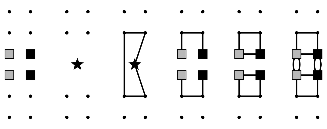
We repair the parity constraint and the $\mathcal{P}$-connectivity constraint independently. Let $T:=\operatorname{odd}(H)\triangle Q$. Since $Q,\operatorname{odd}(H)\subseteq I$ and both have even cardinality, $T$ is an even-cardinality subset of $I$. We compute a minimum $T$-join $J$; then $\operatorname{odd}(H\uplus J)=\operatorname{odd}(H)\triangle T=Q$, so parity is restored. To restore the $\mathcal{P}$-connectivity constraint, for each set $C\in\mathcal{P}$, choose a representative $c_{C}\in C$ and define $\mathcal{D}:=\{\{c_{C},v\}:C\in\mathcal{P},\ v\in C\setminus\{c_{C}\}\}$. We compute a Steiner forest $K$ for the demand pairs in $\mathcal{D}$. Then $K$ connects all vertices in each set $C\in\mathcal{P}$, and adding two copies of $K$ does not change parity. The final edge multiset is $F_{\mathrm{bas}}:=H\uplus J\uplus K\uplus K$. The complete procedure is summarized in Algorithm 1 and illustrated in Figure 2.

The laminar families $\mathcal{L}_{T}$ and $\mathcal{L}_{\mathcal{D}}$ computed in Algorithm 1 will be used as inputs to the dynamic program in Section 4. Let $F^{*}$ be an optimum solution to the input PC-$\Phi$-TSP instance and set $\mathrm{OPT}:=\ell(F^{*})+\pi_{V}^{\Phi}(F^{*})$. We now analyze the approximation guarantee of Algorithm 1.

The proof is given in Appendix A. It uses three simple facts. $F^{*}$ induces a solution to the auxiliary PCTSP instance of value at most $\mathrm{OPT}$, so $\ell(H)+\pi_{V}^{\Phi}(H)\leq\rho\mathrm{OPT}$. Also, $H\uplus F^{*}$ contains a $T$-join of length at most $\ell(H)+\ell(F^{*})$, giving $\ell(J)\leq(\rho+1)\mathrm{OPT}$. Finally, since $F^{*}$ connects every set $C\in\mathcal{P}$, it contains a Steiner forest for the demand pairs $\mathcal{D}$ of length at most $\ell(F^{*})$, and weak duality gives $\sum_{S\in\mathcal{L}_{\mathcal{D}}}y_{S}^{\mathcal{D}}\leq\ell(F^{*})\leq\mathrm{OPT}$.

The second algorithm is a dynamic program that, given a PC-$\Phi$-TSP instance with interface $\Phi=(I,Q,\mathcal{P})$, a fixed constant $h$, an explicitly given laminar family $\mathcal{L}$, and a $\beta$-approximation algorithm $\mathcal{A}_{\beta}$ for the PC-$\Phi$-TSP that runs in polynomial time on instances whose number of prescribed vertices is bounded by a fixed constant, returns a feasible solution in polynomial time when $|I|$ and $\operatorname{width}(\mathcal{L})$ are bounded by constants. As in [21], the dynamic program guesses edges in an optimum solution; larger $h$ allows more such edges to be guessed, but increases the running time. In Section 5, we apply the algorithm to $\mathcal{L}_{T}$ and $\mathcal{L}_{\mathcal{D}}$ computed by Algorithm 1.

The dynamic program constructs and solves instances on certain subgraphs of the given graph. To avoid notational confusion, we call them local PC-$\Psi$-TSP instances, where $\Psi$ denotes the local interface. For $S\subseteq V$, a local interface on $S$ is a triple $\Psi=(I_{\Psi},Q_{\Psi},\mathcal{P}_{\Psi})$, where $I_{\Psi}\subseteq S$, $Q_{\Psi}\subseteq I_{\Psi}$ has even cardinality, and $\mathcal{P}_{\Psi}$ is a partition of $I_{\Psi}$. The corresponding local PC-$\Psi$-TSP instance is the instance on $G[S]$ with local interface $\Psi$. A local feasible solution for this instance is an edge multiset $F\subseteq E(S)$ such that $(I_{\Psi}\cup V(F),F)$ satisfies the parity, $I_{\Psi}$-connectivity, and $\mathcal{P}_{\Psi}$-connectivity constraints for $\Psi$. Its local objective value is $\ell(F)+\pi_{S}^{\Psi}(F)$.

We now describe the dynamic program. Fix a PC-$\Phi$-TSP instance with $\Phi=(I,Q,\mathcal{P})$, a laminar family $\mathcal{L}$, and a fixed positive integer $h$. Let $w:=\operatorname{width}(\mathcal{L})$ and set $B:=|I|+h(w+1)$. For every set $S\in\mathcal{L}\cup\{V\}$, the dynamic program enumerates all local interfaces $\Psi$ on $S$ with $|I_{\Psi}|\leq B$, including the empty interface $(\emptyset,\emptyset,\emptyset)$. For each such interface $\Psi$, it computes a feasible solution $Z[S,\Psi]$ to the corresponding local PC-$\Psi$-TSP instance. The sets $S\in\mathcal{L}\cup\{V\}$ are processed in increasing order of $|S|$. At the end, the algorithm returns $Z[V,\Phi]$, which is a feasible solution to the input PC-$\Phi$-TSP instance. When $k,h,w$ are fixed and $|I|\leq k$, the number of enumerated interfaces with $|I_{\Psi}|\leq B$ is polynomial in $|V|$.

When a set $S\in\mathcal{L}\cup\{V\}$ is processed, the order above ensures that all local solutions $Z[S^{\prime},\Psi^{\prime}]$ with $S^{\prime}\in\mathcal{L}$, $S^{\prime}\subsetneq S$, and $|I_{\Psi^{\prime}}|\leq B$ have already been computed. For each enumerated interface $\Psi_{S}=(I_{S},Q_{S},\mathcal{P}_{S})$ on $S$, the algorithm enumerates all child decompositions of $S$. A child decomposition is a possibly empty pairwise disjoint collection $S_{1},\ldots,S_{p}$ of sets of $\mathcal{L}$ with $S_{i}\subsetneq S$ for every $i=1,\ldots,p$. If $S$ contains no set $S^{\prime}\in\mathcal{L}$ with $S^{\prime}\subsetneq S$, then the empty child decomposition is the only child decomposition. Let $S_{0}:=S\setminus\bigcup_{i=1}^{p}S_{i}$. We call $S_{0}$ the residual part and call $S_{0},S_{1},\ldots,S_{p}$ the parts of this child decomposition. Since every child decomposition contains at most $w$ sets, the number of child decompositions for a fixed $S$ is at most $(|\mathcal{L}|+1)^{w}$, which is polynomial for fixed $w$ because $\mathcal{L}$ is laminar and $|\mathcal{L}|=O(|V|)$.

For the chosen child decomposition, the algorithm enumerates all boundary multisets. A boundary multiset is an edge multiset $X\subseteq E(S)$ such that each edge of $X$ has endpoints in two distinct parts among $S_{0},S_{1},\ldots,S_{p}$, and $|X\cap\delta(S_{i})|\leq h$ for every $i=1,\ldots,p$. Since $p\leq w$, we have $|X|\leq hw$, so the number of possible boundary multisets is polynomial in $|V|$ when $h$ and $w$ are fixed.

For each boundary multiset $X$ and each $i=0,\ldots,p$, set $I_{i}:=(I_{S}\cup V(X))\cap S_{i}$ and $Q_{i}:=I_{i}\cap(Q_{S}\triangle\operatorname{odd}(X))$. If there exists $i\in\{0,\ldots,p\}$ such that $|I_{i}|>B$ or $|Q_{i}|$ is odd, this choice of $X$ is rejected and the algorithm proceeds to the next boundary multiset. Otherwise, the algorithm enumerates all partitions $\mathcal{P}_{i}$ of $I_{i}$ for which $\Psi_{i}=(I_{i},Q_{i},\mathcal{P}_{i})$ is an interface on $S_{i}$ for every $i=0,\ldots,p$. For $i=1,\ldots,p$, let $F_{i}:=Z[S_{i},\Psi_{i}]$, which has been computed since $|I_{i}|\leq B$ and $S_{i}\subsetneq S$. The residual part $S_{0}$ is handled by applying $\mathcal{A}_{\beta}$ to the local PC-$\Psi_{0}$-TSP instance on $G[S_{0}]$; let $F_{0}$ be the returned edge multiset. We compute $F^{\prime}:=X\uplus F_{0}\uplus F_{1}\uplus\cdots\uplus F_{p}$. If $F^{\prime}$ is feasible for the local PC-$\Psi_{S}$-TSP instance on $G[S]$, we keep $F^{\prime}$ as a candidate.

Among all candidates constructed over all enumerated choices for the local PC-$\Psi_{S}$-TSP instance on $G[S]$, the dynamic program chooses one with minimum local objective value and denotes it by $Z[S,\Psi_{S}]$. The empty child decomposition always produces a candidate: then $S_{0}=S$ and $X=\emptyset$, and choosing $\mathcal{P}_{0}=\mathcal{P}_{S}$ gives $\Psi_{0}=\Psi_{S}$, so $\mathcal{A}_{\beta}$ is applied to the local PC-$\Psi_{S}$-TSP instance on $G[S]$. Hence, for every enumerated interface $\Psi_{S}$ on $S$ with $|I_{\Psi_{S}}|\leq B$, the solution $Z[S,\Psi_{S}]$ is defined after $S$ is processed. Since $Z[V,\Phi]$ is defined when the algorithm terminates, the dynamic program returns a feasible solution to the input instance.

The complete procedure is summarized in Algorithm 2 and illustrated in Figure 3.

For fixed $k,h$, Algorithm 2 runs in polynomial time on instances with $|I|\leq k$ when applied to either $\mathcal{L}_{T}$ or $\mathcal{L}_{\mathcal{D}}$, assuming that $\mathcal{A}_{\beta}$ runs in polynomial time on instances whose number of prescribed vertices is bounded by a fixed constant. Indeed, Lemma 3.2 gives $w=\operatorname{width}(\mathcal{L})\leq|I|\leq k$ in these applications, and hence $B=|I|+h(w+1)$ is bounded by a fixed constant. For fixed $B,h,w$, the numbers of local interfaces, child decompositions, boundary multisets, and partition choices are polynomial in $|V|$, so Algorithm 2 considers polynomially many $F^{\prime}$. Each call to $\mathcal{A}_{\beta}$ is made on a local PC-$\Psi$-TSP instance with $|I_{\Psi}|\leq B$, so runs in polynomial time.

Fix an optimum solution $F^{*}$. For $S\subseteq V$, define the interface $\Psi_{S}^{*}$ induced by $F^{*}$ on $S$. Let $I_{S}^{*}:=(I\cup V(F^{*}\cap\delta(S)))\cap S$ and $Q_{S}^{*}:=I_{S}^{*}\cap\operatorname{odd}(F^{*}[S])$. Then $Q_{S}^{*}$ has even cardinality. If $S=V$, set $\mathcal{P}_{S}^{*}:=\mathcal{P}$; otherwise, let $\mathcal{P}_{S}^{*}:=\{D\cap I_{S}^{*}:D\text{ is a connected component of }(I_{S}^{*}\cup V(F^{*}[S]),F^{*}[S])\text{ and }D\cap I_{S}^{*}\neq\emptyset\}$. Write $\Psi_{S}^{*}:=(I_{S}^{*},Q_{S}^{*},\mathcal{P}_{S}^{*})$. In particular, $\Psi_{V}^{*}=\Phi$. By construction, $F^{*}[S]$ is feasible for the local PC-$\Psi_{S}^{*}$-TSP instance on $G[S]$. Define $\mathcal{L}(F^{*},h):=\{L\in\mathcal{L}:1\leq|F^{*}\cap\delta(L)|\leq h\}$ and $F^{*}(\mathcal{L},h):=F^{*}\cap\bigcup_{L\in\mathcal{L}(F^{*},h)}\delta(L)$. Thus $\mathcal{L}(F^{*},h)$ consists of the sets in $\mathcal{L}$ crossed by $F^{*}$ between one and $h$ times, and $F^{*}(\mathcal{L},h)$ consists of the edges of $F^{*}$ crossing at least one such set. The edges in $F^{*}(\mathcal{L},h)$ are the edges Algorithm 2 tries to guess. As $h$ increases, $F^{*}(\mathcal{L},h)$ may contain more edges of $F^{*}$. Figure 4 illustrates $\mathcal{L}(F^{*},h)$ and $F^{*}(\mathcal{L},h)$.

Consider the run of Algorithm 2 on input $(G,\ell,\pi,\Phi,\mathcal{L},h;\mathcal{A}_{\beta})$, where $\mathcal{A}_{\beta}$ is as specified above. We use the following lemmas.

References

- [1] H.-C. An, R. Kleinberg, and D. B. Shmoys. Improving Christofides’ algorithm for the - path TSP. Journal of the ACM, 62(5):34:1–34:28, 2015.
- [2] A. Archer, M. H. Bateni, M. T. Hajiaghayi, and H. Karloff. Improved approximation algorithms for prize-collecting Steiner tree and TSP. SIAM Journal on Computing, 40(2):309–332, 2011.
- [3] A. Archer and A. Blasiak. Improved approximation algorithms for the minimum latency problem via prize-collecting strolls. In Proceedings of the 21st Annual ACM-SIAM Symposium on Discrete Algorithms (SODA), pages 429–447, 2010.
- [4] E. Balas. The prize collecting traveling salesman problem. Networks, 19(6):621–636, 1989.
- [5] D. Bienstock, M. X. Goemans, D. Simchi-Levi, and D. P. Williamson. A note on the prize collecting traveling salesman problem. Mathematical Programming, 59:413–420, 1993.
- [6] J. Blauth and M. Nägele. An improved approximation guarantee for prize-collecting TSP. In Proceedings of the 55th Annual ACM Symposium on Theory of Computing (STOC), pages 1848–1861, 2023.
- Blauth et al. [2026] J. Blauth, N. Klein, and M. Nägele. A better-than-1.6-approximation for prize-collecting TSP. Mathematical Programming, 216:87–109, 2026.
- [8] J. Cheriyan, Z. Friggstad, and Z. Gao. Approximating minimum-cost connected -joins. Algorithmica, 72(1):126–147, 2015.
- [9] K. Chaudhuri, B. Godfrey, S. Rao, and K. Talwar. Paths, trees, and minimum latency tours. In Proceedings of the 44th Annual IEEE Symposium on Foundations of Computer Science (FOCS), pages 36–45, 2003.
- [10] N. Christofides. Worst-case analysis of a new heuristic for the travelling salesman problem. Technical Report 388, Graduate School of Industrial Administration, Carnegie Mellon University, 1976.
- [11] M. X. Goemans. Combining approximation algorithms for the prize-collecting TSP. arXiv:0910.0553, 2009.
- [12] M. X. Goemans and D. P. Williamson. A general approximation technique for constrained forest problems. SIAM Journal on Computing, 24(2):296–317, 1995.
- [13] C. Gottschalk and J. Vygen. Better --tours by Gao trees. Mathematical Programming, 172(1–2):191–207, 2018.
- [14] J. A. Hoogeveen. Analysis of Christofides’ heuristic: Some paths are more difficult than cycles. Operations Research Letters, 10(5):291–295, 1991.
- [15] A. R. Karlin, N. Klein, and S. Oveis Gharan. A deterministic better-than- approximation algorithm for metric TSP. In Proceedings of the 24th International Conference on Integer Programming and Combinatorial Optimization (IPCO), pages 261–274, 2023.
- [16] A. R. Karlin, N. Klein, and S. Oveis Gharan. A (slightly) improved approximation algorithm for metric TSP. Operations Research, 72(6):2543–2594, 2024.
- [17] A. V. Karzanov. How to tidy up a symmetric set-system by use of uncrossing operations. Theoretical Computer Science, 157(2):215–225, 1996.
- [18] A. Schrijver. Combinatorial Optimization: Polyhedra and Efficiency. Springer, Berlin, 2003.
- [19] A. Sebő. Eight-fifth approximation for the path TSP. In Proceedings of the 16th International Conference on Integer Programming and Combinatorial Optimization (IPCO), pages 362–374, 2013.
- [20] A. Sebő and A. van Zuylen. The salesman’s improved paths through forests. Journal of the ACM, 66(4):28:1–28:16, 2019.
- [21] V. Traub, J. Vygen, and R. Zenklusen. Reducing path TSP to TSP. SIAM Journal on Computing, 51(3):STOC20–24–STOC20–53, 2022.
- [22] J. Vygen. Reassembling trees for the traveling salesman. SIAM Journal on Discrete Mathematics, 30(2):875–894, 2016.
- [23] Z. Xu and B. Rodrigues. A 3/2-approximation algorithm for the multiple TSP with a fixed number of depots. INFORMS Journal on Computing, 27(4):636–645, 2015.
- [24] R. Zenklusen. A 1.5-approximation for path TSP. In Proceedings of the 30th Annual ACM-SIAM Symposium on Discrete Algorithms (SODA), pages 1539–1549, 2019.