kokorev24aK24 \defcitealiasakins24aA24
Dust in the Average Galaxy: Attenuation, Emission, and Opacity from
Abstract
We present constraints on the dust emission and attenuation properties of galaxies across using JWST imaging from the COSMOS-Web Survey combined with deep FIR/(sub)millimeter data from Spitzer, Herschel, SCUBA-2, NIKA-2 and ALMA. We analyze over 500,000 galaxies to independently constrain attenuation as inferred in the rest-frame UV/optical as well as dust emission from stacked FIR SEDs, enabling a direct comparison between the two. We find UV/optical attenuation systematically underpredicts IR luminosity by a factor of 3 at and up to an order of magnitude for M⊙. We derive empirical relationships for the effective attenuation (AUV and AV), dust temperature, fraction of star formation that is unobscured, and dust-to-stellar mass ratio as functions of redshift and stellar mass. On galaxy-integrated scales, we separate the first order effect of star/dust geometry from dust grain properties by combining constraints on the IR SED, the UV SED, and the dust mass surface density. Importantly, we measure over an order of magnitude decrease in — the ratio of dust mass absorption coefficients in the UV at 1600Å and FIR at 500m — from to . A depressed ratio is consistent with a deficit of small dust grains, possibly attributable to the intense radiation fields of high- star formation; indeed, we find a redshift-invariant inverse relationship between and . Assuming the varying dust opacity is dominated by changes to small grains and not large grains, we infer a modest evolution in the dust-to-stellar mass ratio with secondary stellar mass dependence, . Most evolution in the dust-to-stellar ratio is at , the product of mild downward evolution in the dust-to-gas ratio combined with steep evolution in the gas-to-stellar ratio. The significant evolution and dynamic range of and prevailing disconnect between the UV/optical and FIR regimes emphasize that direct dust constraints are irreplaceable for the majority of star-forming galaxies at , not just the most extreme star-formers.
keywords:
Galaxies, Attenuation, Dust1 Introduction
Dust makes up a negligible fraction of the cosmic mass budget (%), and yet it has a profound impact on the perception of starlight via attenuation (Salim and Narayanan, 2020; Schneider and Maiolino, 2024). While dust efficiently absorbs ultraviolet and optical photons and converts them to thermal energy re-radiated at much longer wavelengths, our ability to fully characterize interstellar dust beyond our immediate neighborhood has been severely limited by observational hurdles and degeneracies. Dust extinction measurements are limited to individual stellar sightlines in the Milky Way relative to localized measurements of the hydrogen column density (Reina and Tarenghi, 1973; Gorenstein, 1975; Predehl and Schmitt, 1995; Güver and Özel, 2009). Dust attenuation curves have been constrained for nearby galaxies and increasingly larger samples out to (Reddy et al., 2015; Shivaei et al., 2020; Battisti et al., 2022), but the inference relies on assumptions – empirical effective laws (Calzetti et al., 2000), specific star/dust geometries, or fixed grain populations – that have not been independently tested. Direct comparison between attenuation derived from the UV/optical and absorption derived from the FIR remains rare. Dust in emission has been seen predominantly in the rarest of bright submillimeter galaxies (e.g. Smail et al., 1997, see reviews by Blain, Smail, Ivison, Kneib, and Frayer 2002 and Casey, Narayanan, and Cooray 2014a), with relatively little understanding as to how exceptional that dust emission is relative to more ‘normal’ galaxies at high redshift.
The framework through which we study dust in the distant universe is thus anchored to nearby universe calibrations, with a limited range of attenuation curves, dust mass absorption coefficients, and assumptions about star/dust geometries. We implicitly assume that these calibrations apply at greater redshifts. If these assumptions are systemically inaccurate, then much of what we infer regarding dust at high redshift may not hold — dust masses may be off by up to an order of magnitude, and even stellar masses could be under/over-estimated based on the application of an inappropriate attenuation law (e.g. McKinney et al., 2025). Furthermore, dust is built from metals and complex molecules, thus its total mass is also inherently linked to the metallicity of the ISM and star formation histories in galaxies (Draine and Li, 2007; Rémy-Ruyer et al., 2014; De Vis et al., 2019). Both metallicity and star formation histories are believed to be quite different for the ‘average’ galaxy at than at (Maiolino et al., 2008; Mannucci et al., 2010; Zahid et al., 2014; Jain et al., 2026): more metal poor and potentially burstier. Observations of dust at these epochs may reveal interesting details about the integrated enrichment and star formation history. Further it may also reveal its future potential for star formation as a key catalyst for gas cooling in molecular clouds.
Studying and calibrating the impact of dust is intrinsically difficult beyond the local universe, given that extraordinary sensitivity is required to understand the ‘normal’ galaxy population. In this paper we place empirical constraints on galaxies’ dust emission and absorption, and the direct relationship between the two, out to using the marriage of improved constraints from the James Webb Space Telescope, JWST, and the Atacama Large Millimeter and submillimeter Array, ALMA, combined with other FIR datasets, together in the COSMOS field (Scoville et al., 2007). By pushing near-infrared imaging more than 10 deeper than previous imaging at high spatial resolution over large areas, JWST has revolutionized the precision at which we characterize galaxies’ photometric and spectroscopic redshifts as well as the intrinsic shape of galaxies’ rest-frame optical SEDs (Shuntov et al., 2025). This in turn also dramatically improves constraints on their star formation histories (Arango-Toro et al., 2025) and stellar masses measurements. JWST fundamentally pushes this characterization of the rest-frame UV/optical for more galaxies per unit area on the sky, and for galaxies much fainter (1-2 magnitudes) than previously possible. ALMA, along with other (sub)mm facilities, adds constraints on galaxies’ dust emission. The wealth of ALMA data in JWST-imaged areas has ballooned in recent years, such that many galaxies less luminous than traditional dusty star-forming galaxies are now routinely accessible. Furthermore, large areas in the COSMOS field now have deep ALMA continuum maps, enabling truly sensitive stacking experiments propelled in sensitivity by the density of JWST-detected galaxies on the sky.
This paper is organized as follows. § 2 provides a framework for understanding the goals of this work; it discusses the physical relationship between attenuation and emission, and discusses key unknowns. § 3 presents the JWST, ALMA, and other submillimeter data used in this work, focused in and around the COSMOS-Web JWST Survey (Casey et al., 2023). § 4 presents the methodology by which we constrain the UV/optical and, independently, the dust SEDs for galaxies measured as a function of stellar mass and redshift through a FIR stacking analysis. § 5 presents a number of key measurements of implied physical characteristics, their evolution, and redshift dependence; this includes properties derived from the UV/optical portion of the SED, properties derived from the stacked dust SEDs in the FIR, and properties that present physical measurements through a combination of the two. § 6 connects the unique constraints presented in the previous section; we focus in particular on applying the framework of § 2 to separate out the impact of star/dust geometry from dust grain properties and comment on the underlying drivers of the evolution in the dust-to-stellar ratio. § 7 concludes. Throughout, we presume a Kroupa IMF (Kroupa, 2001) and a Planck cosmology (Planck Collaboration et al., 2020). All appearances of imply and implies a natural logarithm.
2 Framework & Approach
It is beneficial to revisit fundamental definitions linking galaxies’ dust attenuation to their emission and mass to clarify our aims in this work. The relationship between optical depth , the dust mass absorption coefficient , path length , and dust density , is . From that, it follows that the magnitudes of attenuation and dust mass surface density, , relate via:
| (1) |
This presumes a simple foreground screen of dust in front of a light source (i.e. starlight).
The dust mass absorption coefficient (Weingartner and Draine, 2001; Draine, 2003) encodes the complex absorption properties of different dust grains, and the grain type and size distribution, as a function of wavelength. It may also be broken into two components corresponding to the intrinsic absorptive properties of the dust (, which goes directly into re-radiated thermal emission) and a scattered light component (, accounting for photons of wavelength that are not destroyed, but rather scattered), such that the total . Milky Way dust has significant scattering for UV/optical photons such that (Cardelli et al., 1989). The scattering vs. absorption distinction is crucial in the consideration of narrow sightlines over which extinction is being measured (e.g. in the Milky Way); in the case of integrated light from entire galaxies, is taken entirely as an absorption factor due to all scattered light being accounted for within the galaxy aperture, as discussed in Calzetti et al. (2000).
Generalizing to a mixed star/dust geometry then can be written as:
| (2) |
where the additional term, , we introduce as a wavelength-dependent factor that encodes the star/dust geometry. It may be defined as the ratio of the effective optical depth (, or optical depth of “apparent extinction”, Charlot and Fall 2000) to the physical optical depth, or similarly the ratio of observed (measured using standard techniques in the rest-frame UV/optical) to directly-inferred (inferred by measures of dust mass surface density, ). By its nature, is bounded such that (the following works all explore the crucial role of geometry, though they do not explicitly use the convention we have outlined with ; Disney et al., 1989; Byun et al., 1994; Witt and Gordon, 1996, 2000; Charlot and Fall, 2000; Chevallard et al., 2013; Narayanan et al., 2018; Trayford et al., 2020; Ferrara et al., 2022; Qin et al., 2024; Sommovigo et al., 2026). corresponds to a uniform foreground slab, and for a uniform, optically-thin () slab with stars mixed uniformly throughout. A case where stars are completely decoupled from dust would correspond to (i.e. a background dust screen), but the reality of mixed star/dust geometries is that some emergent starlight usually escapes near the surface, and should not get very close to 0. The impact of is to lessen for a given dust mass surface density, and while can be worked out analytically for some simple toy models (dust screen, dust slab, exponential disks at given inclination, etc.), it will generally not be a function that is easy to directly measure or derive. For example, it is understood that geometry also has a strong wavelength dependence, such that a clumpy ISM with narrow escape channels for starlight results in a grayer attenuation curve (Natta and Panagia, 1984; Calzetti et al., 1994; Witt and Gordon, 2000; Salim and Narayanan, 2020) or bluer rest-frame UV slope (Goldader et al., 2002; Howell et al., 2010; Casey et al., 2014b; Narayanan et al., 2018) for fixed dust mass.
What is known about from observational constraints? The dust mass absorption coefficient has been empirically measured in the Milky Way via the relation:
| (3) |
where is the attenuation per unit hydrogen column density measured for individual stellar sightlines in the Milky Way to be AV/NH 5.3mag cm2 /H (Bohlin et al., 1978; Diplas and Savage, 1994; Güver and Özel, 2009) in the V-band, where a dust-screen is implicitly assumed (). Mdust/ is the dust to hydrogen gas ratio which has some metallicity dependence (Draine and Li, 2007; Rémy-Ruyer et al., 2014); for the Milky Way, solar metallicity, and a uniform dust screen (), this gives cm2 g-1. This is fairly well constrained to 10% under these conditions. For a general metallicity-dependent dust-to-gas ratio, and no metallicity-dependent geometry, one would expect (in the optical where is measured) to scale with metallicity following, e.g., Eq 9 of Draine et al. (2014).
At longer wavelengths, the total dust mass of a galaxy scales linearly with the rest-frame flux density in the optically-thin portion of the spectrum (Hildebrand, 1983):
| (4) |
Here is the rest-frame flux density of a given dust reservoir emitting longward of 250 m (i.e. on the Rayleigh-Jeans tail of dust blackbody emission), is the luminosity distance, is the dust mass absorption coefficient at the frequency where the flux density is inferred (i.e. in the FIR), is the mass-weighted average dust temperature in the reservoir, and is the Planck function evaluated at temperature . The re-radiated spectrum per dust grain is given by111In practice, the Planck function is computed in erg s-1 cm-2 Hz-1 str-1 and the use of in Equation 4 reflects the use of Janskys in the FIR as typical convention. and the total dust luminosity set by ; another factor of 4 arises from the conversion of from specific intensity to a grain-normalized luminosity, and they cancel out.
The optically-thin portion of the dust spectrum typically occurs at rest-frame wavelengths longward of m. For this work, we will use rest-frame 500m emission to anchor dust mass calculations. Here we adopt a dust mass absorption coefficient at 500 m, cm2 g-1 following Clark et al. (2019), and we note that where throughout the FIR/mm regime. Throughout this paper we will refer to as specifically evaluated at 500m, with the Clark et al. (2019) value denoted . Importantly, we emphasize that dust mass coefficients in the FIR are highly uncertain because the FIR lacks direct empirical constraints unlike the UV/optical where attenuation along stellar sightlines can be directly constrained. A suite of foundational grain models (Mathis et al., 1977) calculate from the UV through the submm (Draine and Lee, 1984), and highlight the impact of dust grain morphology — fluffy aggregates vs. bare compact grains — on (Ossenkopf and Henning, 1994; Henning and Stognienko, 1996). These models were updated to include polycyclic aromatic hydrocarbons (PAHs) in Weingartner and Draine (2001); Li and Draine (2001) and Draine (2003) with a complementary analysis on grain shape in Siebenmorgen et al. (2014). Given the lack of direct, empirical constraints on , we conservatively caution that dust masses cannot be known better than within a factor of 2 following the 2 modeling uncertainty on . The dust mass also has a dependence on flux density and presumed dust temperature Tdust via the Planck Function, and there is also a concern about applying single-temperature models to recover the total dust mass, which is discussed in detail in Sommovigo and Algera (2025). However, despite the dependence on dust temperature and flux density precision, the uncertainty of both (20%) are dwarfed by the uncertainty of .
Dust mass can then be translated to dust mass surface density with knowledge of the dust emitting size effective radius, . In practice, resolved dust sizes are not available for large samples of galaxies to high redshift, but for those that exist, FIR sizes and morphologies draw parallel to trends observed in optical light: higher redshift galaxies are smaller and FIR emission broadly appears consistent with Sérsic profiles with (Hodge and da Cunha, 2020). In this work, we will generalize to use galaxies’ measured sizes from JWST NIRCam imaging (rest-frame optical to near-infrared) as a good proxy of their dust sizes for the purpose of calculating dust mass surface densities. We will assert in this work that . This presumption is one of convenience and necessitated by the limitation of current datasets; it could be lifted in the future with improved constraints on that relationship. The factor of accommodates the fact that dust reservoirs are often slightly more compact than their stellar reservoirs and centrally peaked (Conselice, 2014; Mosenkov et al., 2019); while this prefactor is not precisely constrained, the important component of this is that does not evolve in a wildly different manner than , which is not just consistent with recent observations but also theoretical expectation (e.g. Popping et al., 2022). It then follows that dust mass surface density is then given by:
| (5) |
The dominant uncertainty on still comes from the uncertainty on based on the critical size assumption made here (where future observations could change the error budget).
Joining Equations 2 and 5 for attenuation at wavelength in the UV/optical regime gives:
| (6) |
Here the observables from the FIR are , from an SED fit to observed-frame photometric constraints, from high-resolution imaging, and from a detailed SED fit to the UV/optical SED. The dominant uncertainty in this equation comes from the product of which we will set empirical limits on in this work in the UV (=1600).
Following from Eq. 6, it will be handy later in this work to define the term
| (7) |
which represents the ratio of effective attenuation to dust mass surface density. Here, = kpc2 M⊙-1, our fiducial adopted value of the dust mass absorption coefficient at rest-frame 500m in units of kpc2 M⊙-1. This renders a unitless ratio of attenuation to dust mass surface density. In the V-band, Aniano et al. (2012) infer CV = 0.67, and Draine et al. (2014) find CV = 0.74, both based on Milky Way and dust model calibrations assuming a foreground screen.
If the FIR SED of a galaxy can be observed, then the integrated IR luminosity is known (LIR, typically integrated from rest-frame 8–1000 m, but dominated by emission right around 100 m rest-frame), in addition to constraints on dust mass Mdust from the Rayleigh-Jeans tail. While Mdust depends on which traces dust grain properties, the IR luminosity is free of any such dependence. Through energy balance, the IR tells us, objectively, how much light has ultimately been absorbed in the rest-frame UV/optical and reprocessed by dust grains. LIR is simply equal to the difference between the intrinsic UV (and optical) luminosity and the observed LUV. A wealth of literature exists on IRX LIR/LUV where LIR and LUV are both observed quantities (e.g. Meurer et al., 1999) and its relationship to both AUV (Buat et al., 2005; Hao et al., 2011; Cortese et al., 2008) and rest-frame UV slope (Calzetti et al., 1994; Reddy et al., 2006; Gil de Paz et al., 2007; Takeuchi et al., 2012). We can thus draw a direct line between IRX, this ratio of energy output in the IR and UV, and the attenuation that should be seen in the optical if a simple dust screen is assumed:
| (8) |
The coefficient is the ratio of two bolometric correction factors, BC(1600)/BC(FIR), as discussed in Meurer et al. (1999) and McLure et al. (2018). is approximately equal to one, dominated by the bolometric correction in the UV (where 1600Å luminosity does not reflect the total UV light that is absorbed by dust); later in § 6.1 we discuss further and describe how it can be directly inferred for a given UV/optical SED. The second term in Eq. 8 follows from the first, where funobs is the ratio of star-formation that is unobscured relative to the total, i.e. funobsSFRUV/(SFRUV+SFRIR), which is another convenient conceptual way of framing IRX. The coefficient, , then represents the ratio of SFR-to-luminosity scalings222 is used in Kennicutt and Evans (2012) to denote the coefficient between luminosity and SFR, but here we use to be clear this is a different quantity than is denoted in Eq. 7 between the total infrared, TIR, and far ultraviolet, FUV, in Kennicutt and Evans (2012): 1.15.
We can then draw direct comparison between AUV,direct, the attenuation that should be present if all of the dust were concentrated in a screen, and AUV, the effective or ‘observed’ attenuation in the UV. The latter may be derived through detailed UV/optical SED fitting when sufficient constraints are at hand to also constrain the star formation history (there is always some degeneracy between stellar age and attenuation causing redder SEDs in the UV/optical; see review on stellar population synthesis by Conroy, 2013). The difference between AUV,direct and AUV is attributable to geometry alone, such that:
| (9) |
This also follows from dividing Eq. 2 by Eq. 1 in the UV (we will use 1600Å to denote UV in this work). So while the geometry itself is complex, we can use the rest-frame UV to directly parameterize in a global, integrated sense. Then we may combine Eq. 6 with Eq. 8 and Eq. 9 and place constraints on the galaxy-integrated ratio of dust mass absorption coefficients, directly:
| (10) |
Measurement of this ratio can provide some first steps towards a greater understanding of the dust grain properties in the early Universe through a relatively straightforward set of observations. The observables333The framework we discuss takes for granted that redshift, , is reasonably well constrained. here are LIR, LUV, , Tdust and . We also note that the ratio of LIR and form a proxy for Tdust, leaving the number of true independent, observational constraints needed to four. We note that, theoretically, is a microphysical characteristic of dust grain properties, but here we are calculating a quantity linked in meaning, but integrated on macroscopic scales, which inherently folds in second-order effects of ISM geometry, which are complex and not directly measured. While this ratio may still be uncertain within a factor of two or more (again, from uncertainty on ), we can infer if it evolves, which can inform future models of dust grain physics in the early Universe where no direct constraints on exist.
Our work aims to make such measurements, and simultaneously present observations on the evolution and stellar-mass dependence of related quantities: the magnitudes of attenuation in the UV and optical, the effective attenuation law slope, LIR, Mdust and Tdust, the fraction of unobscured star formation relative to total (funobs), and the dust-to-stellar mass ratio. This paper focuses on a stacking analysis, while a future work will focus on the specific characteristics of galaxies that have direct detections in the IR.
3 Data
We use data from the COSMOS-Web Survey (PIs: Kartaltepe & Casey; Casey et al., 2023). The unique combination of depth and area covered by JWST and ALMA datasets in recent years is particularly notable in the COSMOS field, making it the only dataset uniquely capable of this type of measurement: stacking many thousands of galaxies across uniquely diverse (sub)mm datasets.
3.1 JWST Data
The JWST data in COSMOS, which forms the backbone of the dataset used in this paper, is described in the imaging reduction papers presenting NIRCam data (a contiguous 0.54 deg2 in four filters; Franco et al., 2025) and MIRI data (0.2 deg2 taken in parallel; Harish et al., 2025) and the COSMOS-Web “COSMOS2025” catalog description paper (Shuntov et al., 2025). To briefly summarize these data, NIRCam imaging in COSMOS-Web includes four filters (F115W, F150W, F277W, and F444W) with 5 point source depth (in 03 diameter apertures) roughly 27.5-28.2 AB. MIRI includes one filter (F770W) to a 5 point source depth of 25.5-26 AB. The COSMOS2025 catalog was assembled using a NIRCam-only combined detection image, hotcold detection with SEP (Barbary et al., 2016), 2D morphological Sérsic model construction using SE on NIRCam, and fixed model photometric extraction on 37 photometric bands spanning ultraviolet through mid-infrared. The catalog contains 784,016 sources spanning the 0.54 deg2 of NIRCam coverage. Photometric redshifts are fit using LePhare (Arnouts et al., 2002; Ilbert et al., 2006) and a broad range of templates spanning a wide range of attenuations, emission line strengths, and complex star formation histories (see Shuntov et al. 2025 for details on modifications made to LePhare for COSMOS-Web and Arango-Toro et al., 2025, for more detail on CIGALE-derived physical properties of sources in COSMOS2025 and the consistency of those properties with LePhare).
Of the 0.54 deg2 area, 16% of the area (0.086 deg2) is contained within ground-based star masks; in other words, the ground-based photometry in these regions is severely limited by spatial confusion with bright foreground stars that are less problematic in space-based imaging. Space-based photometric redshifts, including only HST and JWST photometry, are generated for all objects in the catalog and these are used in place of the full ground+space redshifts inside of these star masked regions (see Shuntov et al. 2025 for discussion of the broad consistency between ground+space and space-only photometric redshifts).
3.2 (Sub)Millimeter Data
COSMOS has a wealth of (sub)millimeter ([sub]mm) data from which we can derive accurate dust emission constraints. The most notable datasets of competitive depth and unique wavelength coverage include Spitzer/MIPS, Herschel/PACS+SPIRE, SCUBA-2, NIKA-2, and ALMA coverage. Spitzer MIPS 24m imaging (Sanders et al., 2007) covers the full field to 1=16 Jy depth. Herschel PACS 100m and 160m imaging (Lutz et al., 2011) also cover the full field to 2.37 mJy and 4.75 mJy 1 depth, respectively. Similarly, Herschel SPIRE imaging, at 250m, 350m, and 500m (Oliver et al., 2012) is confusion-limited to a 1 RMS of 5.8 mJy, 6.3 mJy and 6.8 mJy respectively. SCUBA-2 imaging in the field is described by Simpson et al. (2019), which has 1 depth ranging from 0.6–1.4 mJy at 870m (while the effective monochromatic flux density of the filter is 870m, the filter is often referred to as 850m). NIKA-2 data in the field covers an area of 0.3 deg2 (Carvajal-Bohorquez et al., 2026; Béthermin et al., 2026) mostly overlapping the COSMOS-Web area; maps at 1.3 mm and 2 mm have 1 depths of 0.32 mJy and 0.091 mJy, respectively, with corresponding spatial resolutions of 11′′ and 17′′.
Finally, ALMA data, though not exhaustive or uniform, covers a large number of sources at different frequencies and depths. The two roughly uniform blank-field survey datasets used in this work are the Ex-MORA survey (Long et al., 2026, a continuation of the MORA survey described in Casey et al. 2021 and Zavala et al. 2021), a 2 mm deep field (1 90 Jy at 2.1 mm) covering 0.16 deg2, and the CHAMPS survey (Faisst et al., in prep, Martinez et al., in prep Zavala et al., 2026), a 1.2 mm mosaic (10.14 mJy) covering the 0.2 deg2 of JWST MIRI imaging in the field from COSMOS-Web and PRIMER (Donnan et al., 2024).
Beyond these blank-field efforts, we make use of the A3COSMOS444See https://sites.google.com/view/a3cosmos survey (Liu et al., 2019; Adscheid et al., 2024) to formulate a complete list of individual dust detections in the field, combining data from the SCUBA-Dive project (McKinney et al., 2024) on the brightest submm galaxies in the field, to CHAMPS, and Ex-MORA detections. The A3COSMOS dataset (in particular the 2025-03-12 data release) contributes most of the direct detection sources: 725 out of a total of 1024 across the field. In the stacking analysis that follows we keep track of these individual detections and their influence on the results but save analysis of their characteristics to a future work.
4 Methods
Here we present the derivation of physical parameters closely associated with dust emission and absorption. To do this, we treat dust emission and dust absorption independently. The former is measured in the submm and the latter is measured from the rest-frame UV/optical portion of the SED. This is complementary to, though different than, common efforts that use energy balance techniques to fit both portions of the spectrum simultaneously. Energy balance approaches directly translate absorbed rest-frame UV/optical light to re-radiated FIR/millimeter emission (Silva et al., 1998; da Cunha et al., 2008, 2015; Burgarella et al., 2005; Noll et al., 2009; Boquien et al., 2019). Such energy balance techniques, though insightful, rely on some key assumptions we aim to break down empirically in this work: fixed (or relatively inflexible) attenuation laws, fixed dust mass absorption and emissivity assumptions, as well as fundamental presumptions made regarding star/dust geometry. By not enforcing energy balance, we are able to compare the inferred attenuation to the output LIR and assess, under what conditions, the UV/optical SED accurately recovers re-radiated dust emission.
In what follows we first describe the selection and pruning of galaxies in the COSMOS-Web catalog for stacking in FIR/(sub)mm datasets in § 4.1. Note that we explicitly aim to exclude quiescent systems from our stacks for ease of physical interpretation; at high masses and low redshifts, a significant population of quiescent galaxies are known to have markedly different dust characteristics than mass-matched galaxies with higher star-formation rates, with quiescent galaxies showing both suppressed dust emission and absorption (e.g. Paspaliaris et al., 2023; Chang et al., 2026). So it is in the interest of not mixing physically distinct populations – quenched systems and star forming systems – that we restrict to those thought to have dust warmed by the interstellar radiation field generated from star formation.
We then describe the IR SED fitting procedure to the stacked SEDs in § 4.2. Finally, we bootstrap the COSMOS2025 catalog to re-derive flexible attenuation law characteristics using priors based on the COSMOS2025 photometric redshifts (§ 4.3).
4.1 Stacking
Of 784,016 sources in the COSMOS-Web catalog, only 1024 (0.1%) currently have direct detections in the FIR/(sub)mm. Those individual galaxies are a focus of a separate work. We use submm stacking to characterize the dust properties of a broader dynamic range of ‘normal’ galaxies here. Submillimeter stacking is not a new enterprise (for example, Dole et al., 2006; Pascale et al., 2009; Penner et al., 2011; Viero et al., 2013; Béthermin et al., 2015a; Coppin et al., 2015; Tacconi et al., 2018; Inami et al., 2020; Magnelli et al., 2020). However, the limits of stacking results (in redshift, IR-luminosity, and mass) are dependent both on the size of the sample being stacked, and the precision with which its characteristics (like redshift, mass) are known, and the depth and wavelength of the (sub)mm data used in the stacking. JWST has taken us into a new realm of stackable samples: the on-sky density of galaxies has increased significantly, both at higher redshifts and for lower mass galaxies. JWST data has also significantly improved galaxies’ photometric redshifts, improving the purity of stackable samples (Shuntov et al., 2025). Similarly, ALMA has now built up significant (sub)mm datasets to competitive depths such that stacking of yet-unreached mass regimes is now possible. ALMA also has more long wavelength data (1 mm) than single-dish facilities that have covered wide areas (like Herschel, SCUBA-2); the long wavelengths, as well as ALMA-like depths at those wavelengths, are crucial for measuring reliable dust masses out to high redshifts (because they still probe the regime where the dust SED is still safely optically thin, longward of rest-frame 250 m).
The FIR/(sub)millimeter data we stack in this analysis includes: Spitzer MIPS-24m (Sanders et al., 2007), Herschel-PACS 100m and 160m maps (Lutz et al., 2011), Herschel-SPIRE 250m, 350m, and 500m maps (Oliver et al., 2012), SCUBA-2 850m (Simpson et al., 2019), NIKA-2 1.3mm and 2mm (Carvajal-Bohorquez et al., 2026; Béthermin et al., 2026), CHAMPS 1.2mm (Martinez et al., Faisst et al., in prep), and Ex-MORA 2mm (Long et al., 2026).
We stack these datasets by stellar mass and photometric redshift as presented in the COSMOS2025 catalog (Shuntov et al., 2025). We first apply some basic filtering of the COSMOS2025 catalog to remove sources of potential low quality. Of the 784,016 sources in the catalog, we select those with:
-
1.
mag_model_f277w 28.2 &
-
2.
warn_flag = 0 &
-
3.
((chi_star/chi2_best) 1 OR
(radius_sersic3600) -2.3) & -
4.
(flag_star_hsc = 0 OR zpdf_med-zpdf_med_space/(1+zpdf_med) 0.15) &
-
5.
zpdf_u68-zpdf_l68/(1+zpdf_med) 3
The first criterion selects sources brighter than the nominal 5 point source detection limit in the deepest COSMOS-Web band; the second criterion selects non-flagged sources (see Shuntov et al., 2025, for flagging details, mostly related to artifacts). The third criterion serves to exclude Milky Way stars from analysis: unresolved point sources where the . This is a bit more conservative than the stellar flag included in the COSMOS-Web catalog public release to prevent marginal or unclear sources from entering the stackable galaxy population. The fourth criterion requires a source lie outside the HSC star mask region (where ground-based data is potentially faulty due to bright star contamination) or, if within the HSC star mask region, that there is close agreement between the redshift solutions found with and without exclusion of the ground-based photometric constraints. The last criterion down-selects to sources without significant bimodality in their redshift PDFs. This filtering of the catalog produces a set of 595,351“stackable” sources (accounting for 79.6% of the COSMOS2025 catalog).
We make two final cuts to the set of stackable sources. The first cut removes sources with suspiciously high stellar mass estimates for their photometric redshift. To do this we calculate a mass threshold above which sources should be regarded with suspicion for formation within CDM. We determine this redshift-dependent mass threshold using the Sheth and Tormen (1999) halo mass function and calculate the most massive object expected in a given redshift bin (of width ) in the 0.54 deg2 area of the survey, assuming that source has converted 30% of its baryons to stars (following the same logic as in Boylan-Kolchin, 2023). The threshold of a 30% conversion exceeds typical expectation for the efficiency of star formation of, at most, % (e.g. Evans et al., 2009; Bigiel et al., 2010; Thompson et al., 2005; Ostriker and Shetty, 2011). Objects with masses higher than this redshift-dependent maximum mass limit are excluded from the stacks. There are 142 such sources above the limit, likely because their photometric redshifts are overestimated; alternatively their stellar masses may be overestimated due to significant non-stellar contributions to their SEDs. Whatever the origin, we make the conservative choice of cutting them out of the stacking process.
One final, important cut is made to remove quiescent galaxies. Galaxies at low redshifts and high stellar masses follow a bimodal division where the dust characteristics of star-forming massive galaxies are quite a bit different than for quiescent massive galaxies (Paspaliaris et al., 2023). We expect dust emission in the former and not the latter (Toni et al., 2026). We cut out quiescent systems using a SFR cut with respect to the galaxy main sequence, or SFR-M⋆ relation. For a given zpdf_med and mass_med (i.e. and M⋆), we calculate the expected main sequence SFR “SFRMS” using the Speagle et al. (2014) parameterization and excludes sources that are more than a dex lower than the main sequence. In other words, retained sources have SFRSFRMS/10; this includes all sources down to an order of magnitude below the main sequence. This reduces the total stackable star-forming galaxy sample to 501,656 sources (64.0% of COSMOS2025). The distribution of sources in the redshift, mass plane is shown in Figure 1, along with the mass and redshift bins used in this work ( and ).
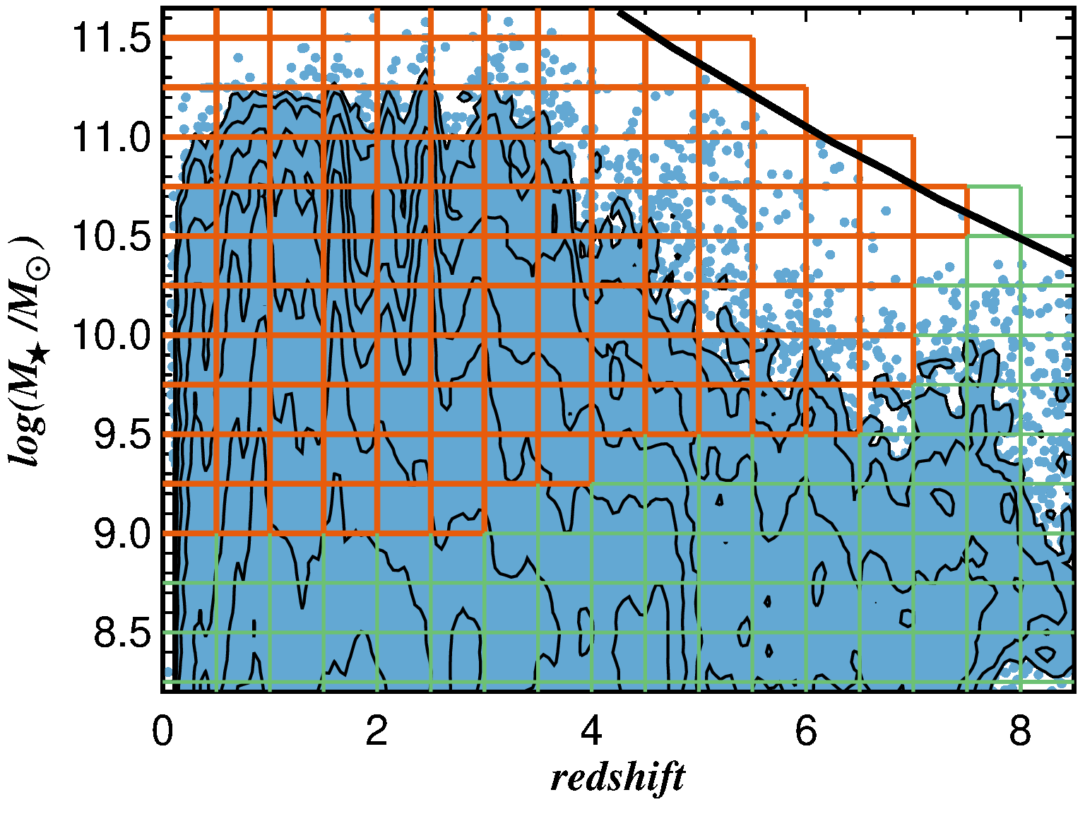
We note that all stackable sources are covered by MIPS, PACS, SPIRE and SCUBA-2 maps. There are 351,222 of those within the NIKA2 1.3 mm map footprint, and 348,503 in the NIKA2 2 mm map footprint. Similarly there are 209,320 sources covered in the CHAMPS map and 149,685 in the ExMORA map. These numbers are reflective of the area within COSMOS-Web covered by each survey.
Note that we do not explicitly exclude any additional special category of source from this list of stackable sources. Both X-ray AGN and submillimeter luminous galaxies are included as a result. We have relatively few concerns about ‘contamination’ of IR flux by the former. Luminous X-ray AGN do correlate somewhat with IR luminous galaxies (Iwasawa et al., 2011), however the wavelengths of light we are stacking predominantly correspond to cold ISM dust. Constraints in the mid-infrared, where an AGN might boost the luminosity substantially, are very weak relative to the longer-wavelength, cold dust constraints. The primary concern regarding AGN is their impact on a galaxy’s SED-modeled stellar mass (Ciesla et al., 2015; Florez et al., 2020; Buchner et al., 2024), such that stellar masses may be overestimated with inclusion of buried AGN luminosity in the UV/optical SED fitting. This is likely a persistent issue, indeed, and the fix for it would involve a very careful analysis of AGN content of the galaxies being stacked, which is beyond the scope of this work. However, we note that AGN luminosity (via the black hole accretion rate density) follows the star formation rate density evolution closely (Delvecchio et al., 2014; Madau and Dickinson, 2014), suggesting that whatever the systematic offset is for stellar masses due to AGN, it is likely to be uniform and smoothly evolving over the redshift and mass range studied.
The inclusion of IR luminous galaxies (e.g. DSFGs broadly defined) is a potential contaminant some readers may worry about as it is possible their IR flux densities are significantly elevated above the norm. To check the impact of the IR luminous population, we have run two versions of our stacks: one with the 1024 direct detections explicitly removed and one including them. We find our stacking results, with and without DSFGs, consistent within errors and attribute this to the relative on-sky rarity of IR luminous galaxies compared to the size of the samples used in the stacking (1024/501,6560.2%). The bins that are most substantially affected (where 50% of the stackable sample is removed) are at , though the resulting flux densities are consistent within (large) errors. For the sake of simplicity in our measurements, and in the interest of avoiding cherry-picking the stacked sample, we proceed in our analysis without excluding IR luminous galaxies.
Our stacked flux densities are measured via a weighted inverse-variance median based on the RMS of the (sub)mm datasets (not the quality of the redshift or stellar mass estimates). Because we are not accounting for redshift uncertainties, we will point out that there will be some level of ‘bin-smearing’ in bins where the photometric redshift quality is a bit worse. This happens at the low-mass and high- end of our stacks where is of order the bin size; the vast majority of bins have somewhat precise photometric redshift uncertainties, , out to . A full description of the stacking procedure, including a comparative analysis of correcting flux densities for clustering bias, is detailed in the Appendix. We note that confusion noise, due to low spatial resolution maps from Herschel or Scuba-2, is greatly mitigated when combining data during a stack as the maps are set to have zero background, a key advantage that lets us push the depth of these maps with sufficient statistics. We provide stacked cutouts as well as a full tabulation of the measured flux densities (Table 30) and derived SED characteristics (Table 30, derivation thereof described below) from the stacked samples above stellar masses 109 M⊙ from in the Appendix555Both tables are available online in fits format at https://github.com/caitlinmcasey/duststacks ..
4.2 Fitting IR Dust SEDs
Our IR SED fitting follows the methodology of MCIRSED described in Drew and Casey (2022), built on earlier SED methodology described in Casey (2012), which joins a single modified blackbody to a mid-infrared powerlaw and fits SEDs to photometry in a Bayesian framework. The model is quite flexible and requires some choices. The free parameters of the dust SED are the following, from best-constrained to least-constrained:
-
1.
the integrated IR luminosity LIR (which determines the normalization of the fit and is canonically integrated between 8–1000m),
-
2.
the luminosity-weighted cold dust temperature Tdust,
-
3.
the emissivity spectral index (which determines the slope of the Rayleigh-Jeans tail of dominant dust blackbody emission),
-
4.
the mid-infrared spectral slope (which determines the relative proportion of warm dust to the dominant cold dust in the SED), and
-
5.
an assumption regarding the opacity of the dust (i.e. at what wavelength the SED transitions from optically thin to thick, ).
In only rare cases — DSFGs with a wealth of IR photometric constraints as well as spatially-resolved IR maps — can all of these parameters be directly constrained. In practice, most galaxies have a tremendous dearth of information in this wavelength regime, so some assumptions must be applied. That is the case for the stacked SEDs.
After extensive testing and evaluation of the resulting SEDs, we decide to uniformly fix the last parameter described above: the wavelength at which opacity shifts from thick to thin (). We use at 100 m, which is consistent with existing constraints in the literature (Draine, 2006; Conley et al., 2011; Greve et al., 2012; Simpson et al., 2017). We note that the choice of impacts the mapping of the rest-frame peak wavelength, , to the dust temperature, Tdust (see Figure 20 of Casey, Narayanan, and Cooray 2014a), but it does not significantly change the shape of the best-fit SED. For example, a similar optically-thin SED fit would produce the same peak wavelength and same LIR, but a correspondingly lower dust temperature. Note that the observables really are and LIR, and our inference of temperature is model dependent. The adopted opacity model, similarly, does not impact dust mass, because the mass is inferred from the optically-thin portion of the dust SED, longward of rest-frame 250 m.
Our constraints on the mid-infrared, governing , come from Spitzer 24m and Herschel PACS. Over a large range of low-redshift SEDs both Spitzer and PACS measurements have high SNR, so we allow to vary as long as there are two or more photometric constraints significant short-ward of rest-frame 200 m. When those constraints are not present, we adopt translating to a moderately steep drop off of the Wien’s side of the dust blackbody. We note this is somewhat steeper than the empirically measured for local (U)LIRGs (U et al., 2012; Casey, 2012), but consistent with many other high- DSFGs (Kirkpatrick et al., 2012; Casey et al., 2014a) and our own measurements in bins where it is explicitly measured: .
Our constraints on the Rayleigh-Jeans tail are quite good below allowing for a direct fit of the emissivity spectral index, . If there are more than two photometric constraints significant at rest-frame wavelengths longward of 300 m, we allow a free fit for . We otherwise fix the value to (Hildebrand, 1983; Dunne and Eales, 2001; da Cunha et al., 2008). This fixed value is consistent with the bins where was directly fit, , as well as other recent literature constraints (Casey et al., 2021; Cooper et al., 2022; Long et al., 2026). While one might be concerned about a comparison of fits with free and to those with fixed values, we note that the dynamic range of both parameters impact the measured LIR by less than 20%.
Photometry is given an additional 10% flux calibration uncertainty and individual stack measurements are capped at a maximum SNR of 10 in order to minimize the statistical power of individual high SNR photometric measurements (e.g. 24m). LIR and Tdust are left as free parameters for all fits. Dust mass is not a parameter fit for explicitly, but inferred directly within the SED fitting and calculated using Eq. 4 for each set of SED parameters. All SED fitting is corrected for CMB heating following the prescriptions provided in da Cunha et al. (2013). A gallery of resulting SED fits over all stacked bins is shown in Figure 2.


4.3 Derivation of Attenuation Characteristics
The primary purpose of the COSMOS2025 catalog is to measure photometric redshifts and, second, to measure basic physical characteristics like rest-frame UV magnitude and stellar mass. Photometric redshift fitting requires a delicate balance of increased free parameters dictating the galaxy template SEDs against obtaining a realistically constrained redshift. The COSMOS2025 approach, more thoroughly described in Shuntov et al. (2025), uses more free parameters than the simplest photometric redshift techniques like EaZY (Brammer et al., 2008). This is done to provide the most realistic estimates on photometric redshift uncertainties; with too few free parameters, the uncertainty is often under-estimated, and with too many it will be overestimated.
A crucial piece of photometric redshift fitting is applying an attenuation law to galaxy templates. So as not to introduce too many free parameters into the fits, COSMOS2025 adopts three possible rigid attenuation laws – the Calzetti et al. (2000) starburst attenuation law, the Arnouts et al. (2013) attenuation law and the Salim et al. (2018) attenuation law – with a range of spanning 0–1.2 in bins of 0.1 magnitudes. This roughly translates to magnitudes of attenuation , with a majority of sources (99%) fit to . Most sources (51%) are fit to the Calzetti et al. (2000) attenuation law, while the remainder are evenly split between the Arnouts et al. (2013) and Salim et al. (2018) laws. This range of choices – quantized choices of and attenuation law – is well suited for the broad application of fitting photometric redshifts. However, in this work we are digging deeper into the attenuation characteristics of galaxies as measured from the UV/optical and to do that, we need some more flexible, direct fits to the primary parameters governing attenuation.
To constrain sources’ attenuation characteristics, we fit detailed SEDs to all COSMOS-Web galaxies’ fiducial model-based photometry using bagpipes (Carnall et al., 2018). We use the BPASS stellar model grids (Eldridge and Stanway, 2009). A Gaussian prior is placed on redshift centered on the median redshift from LePhare (zpdf_med) with standard deviation set to the maximum value of the upper or lower 68th percentiles with hard limits at 3 (or , whichever is more restrictive). A non-parametric star formation history with a continuity prior is used (a -distribution with degrees of freedom =2 and scale = 0.3); twelve bins are used at , nine bins are used at , and seven bins are used at . The four most recent bins have fixed age intervals of 0-10, 10-30, 30-100 and 100-300 Myrs, and the remainder are spaced uniformly in from 300 Myr to . A uniform prior on metallicity is placed between 0–2.5 solar, and nebular emission is fit with uniform prior between .


A flexible attenuation law is modeled with a Salim et al. (2018) parameterization originally presented in Noll et al. (2009), with uniform prior on AV between AV, uniform prior on , the powerlaw deviation from a Calzetti dust law, between (where corresponds roughly to the SMC attenuation curve), and a uniform prior on the 2175Å bump strength between . To reproduce the attenuation curve for a given and , the Calzetti attenuation law, , (specifically equation 4 of Calzetti et al., 2000) is manipulated via equations 3, 4 and 9 in Salim et al. (2018).
We save the posterior median and 68th-percentile confidence intervals on redshift, stellar mass, AV, AUV, (deviation from Calzetti dust law), (bump strength), , and (rest-frame UV slope). AUV and are evaluated at rest-frame 1600Å. We note that, given this is a photometrically-constrained sample with some redshift uncertainty, attenuation characteristics are uncertain on a source-by-source basis: is only well constrained for sources with well-sampled rest-frame UV and optical, while bump strength, is not well constrained in a majority of cases; however we still keep it as a free parameter in an effort to realistically inflate the uncertainties on other attenuation-related quantities.
We verify that bagpipes output is consistent with LePhare-derived characteristics, as shown in Figure 3. The posterior on derived bagpipes redshift differs by , of order the uncertainty on the photometric redshift, without any systematic offset. The derived bagpipes stellar masses are 0.06 dex lower than those from LePhare, slightly less than the average uncertainty on the LePhare stellar mass, of 0.07 dex. Further, we also drew comparison to the stellar masses derived in Arango-Toro et al. (2025) using cigale and find similar consistency. While the LePhare attenuation fits are quantized, they too are broadly consistent with the attenuation fit in bagpipes with a slight skew towards higher magnitudes of attenuation with bagpipes.
5 Results
Here we summarize a number of comparisons between physically-derived galaxy properties. In § 5.1 and § 5.2 we first analyze the results of attenuation characteristics, derived from UV/optical SEDs alone, independent from dust SEDs. We look at the attenuation - stellar mass relation and the implied evolution of inferred attenuation characteristics. Next we analyze galaxies’ FIR SED characteristics, measured independently from UV/optical SEDs. In § 5.3 we show the evolution of LIR and Mdust, and in § 5.4 we show the evolution of dust temperatures. § 5.5 summarizes the measured mid-infrared slope and emissivity spectral index from the dust SED. Finally, we measure quantities that draw both on the results of UV/optical SED fitting and FIR SED fitting; in § 5.6 we analyze the fraction of star formation that is unobscured as a function of stellar mass and redshift, and in § 5.7 we present the mass and redshift dependence of galaxies’ dust-to-stellar (DTS) ratios. Throughout this paper we use a uniform color scheme to show different mass bins evolving with redshift (drawn from the magma color palette) and redshift bins as a function of stellar mass (viridis color palette).
5.1 Attenuation - Mass Relation
The relationship between stellar mass and globally-averaged attenuation has been established in the literature (Devour and Bell, 2016; Bogdanoska and Burgarella, 2020; Qin et al., 2024). The relation exists between stellar mass and AUV as well as AV, where the difference is driven by the underlying nature of the attenuation curve (AUV2.5AV for a Calzetti attenuation curve). We first anchor our measurements to other literature measurements of AUV-M⋆ and proceed to interpret trends we measure across the full range of mass and redshift accessible in our analysis. We emphasize that we are discussing the effective or observed attenuation here, derived from constraints in the UV/optical only.
Figure 4 presents a comparison of our derived relation against literature measurements from 9 and . Plotted are the median values of AUV and 68% spread on AUV values in each bin. At intermediate redshifts (), literature measurements are broadly consistent with our findings within uncertainties; these literature measurements draw specifically on Herschel (Heinis et al., 2014; Pannella et al., 2015) and ALMA-observed (McLure et al., 2018) samples of galaxies, and sources with direct Balmer decrement measurements (Shapley et al., 2022). The primary discrepancy is at the lowest redshifts () where we infer systematically higher median attenuation, AUV for galaxies with stellar mass M⊙ compared to local measurements of AUV in the same mass range (Garn and Best, 2010; Salim et al., 2016). While the median attenuations differ, we note that all literature measures fall well within the inner 68%-ile confidence interval of sample measurements. Note that constraints on AUV in the lowest redshift bin, , in our work will be somewhat more uncertain than both the literature constraints at similar redshifts or our work at higher redshifts because we have not explicitly included GALEX photometric constraints in the COSMOS2025 catalog. Our measurements of AUV-M⋆ suggest little evolution across this mass and redshift range, and broad consistency with the literature, especially at .


Given the relatively good agreement, we present the extended attenuation - stellar mass relationships in fixed redshift bins out to in Figure 5.
While there was little evidence for evolution in AUV-M⋆ out to (Shapley et al., 2022), the data in Figure 5 suggest some slight downward evolution in AUV at fixed stellar mass with increasing redshift out to . The same trend is seen in AV at fixed stellar mass as a function of increasing redshift. The lower AUV and AV is most striking in the mass range from . Higher stellar mass bins show little evolutionary trend, suggesting that non-quenched massive galaxies tend to be quite obscured regardless of redshift.
Both AV-M⋆ and AUV-M⋆ resemble logistic growth functions with a monotonic decline in AUV and AV at fixed stellar mass with redshift (out to ). Thus we fit our binned data to a simplified model describing the average AV expected at a given stellar mass and redshift:
| (11) | ||||
where . We similarly fit this same model to AUV and report the derived parameters for both relations in our appendix, Table 1. We also plot the fitted relation split into individual redshift panels in the appendix.
At redshifts higher than , we see an interesting inflection in the data, such that AUV and AV at fixed stellar mass increase with redshift, where the minimum attenuation is around . The sample scatter on binned AUV and AV are significant, but the increase from to is seen in every mass bin between M⊙. The reason for this reversal is unclear. is the end of reionization, before which the IGM is more optically thick; though our model fitting with Bagpipes lacks a direct implementation of the IGM damping wing (Miralda-Escudé and Rees, 1998) or significant nebular 2-photon continuum contributions (Katz et al., 2024), both of which could artificially redden the spectra of galaxies without dust. Another possibility is that galaxies’ ISM at earlier times may undergo some type of transition around , related to their compact sizes, star/dust geometry, and/or sources of early dust. We will leave a further investigation of this phenomenon – whether physical or an artifact of our SED modeling – to a future work.

5.2 Evolution in the Attenuation Curve
Salim and Narayanan (2020) provide an overview of recent (pre-JWST) results pertaining to the derivation of the attenuation curve, both for low redshift and high redshift samples. To briefly summarize the consensus view, the literature clearly demonstrates that galaxies’ attenuation curves are diverse; there is significant evidence that some star-forming galaxies in the local volume have attenuation curves similar to (if not steeper than) the SMC (Conroy et al., 2010; Leja et al., 2017; Salim et al., 2018) and significantly steeper than the Calzetti attenuation law (Calzetti et al., 2000, see also Battisti et al. 2016), though it is perhaps stellar mass and metallicity dependent in the local volume. Similarly, work beyond from the pre-JWST era suggests steeper-than-Calzetti attenuation laws may be common, but not quite as steep as work on local star-forming galaxies.
Figure 6 highlights our primary finding, that , the deviation of the attenuation law slope from Calzetti, averaged over mass-matched bins shows redshift dependence from to , with especially pronounced evolution seen over . We do not find that has a significant stellar mass dependence though slight mass variance is seen in Figure 6 at fixed redshift, but we caution that lower mass sources are fainter and their attenuation curve slopes are less well constrained (cf. Vijayan et al., 2024). Specifically we find that the average attenuation law steepens with decreasing redshift such that:
| (12) |
This is explicitly fit to all sources above stellar masses M⊙ and where is best constrained. Our results, though of marginal significance (the redshift evolution is 2.1 significant) are consistent with the prior measurements of the attenuation law slope from both (Conroy et al., 2010; Salim et al., 2018) and samples (Buat et al., 2012; Kriek and Conroy, 2013; Reddy et al., 2016), though our data show significant scatter at . We attribute the scatter at low- to a limitation of our data: specifically, the GALEX data was not included in the COSMOS2025 catalog, and thus measurement of our low- attenuation curves are done from extrapolation from the -band blueward. At our photometric data cover the entirety of the rest-frame UV, and correspondingly, the distribution in measured slopes narrows.
We note that our results here are complementary though less constrained than spectroscopic analyses (Markov et al., 2025a, b; Shivaei et al., 2025). We also note that constraints from Balmer decrements (Calzetti et al., 2000; Reddy et al., 2015; Battisti et al., 2022) can differ from SED-fitting methods and favor a steepening of attenuation law with increasing redshift.


5.3 LIR and Mdust
Pivoting in focus to the FIR SEDs, we present the derived IR luminosities and dust masses of our stacked SEDs in Figure 7 split into stellar mass bins to highlight their redshift evolution. We observe a few general trends in the SEDs: at , IR luminosities are exceedingly low, with median LIR1010 L⊙ even for galaxies around masses M⊙. IR luminosities are a factor of 100 brighter around , the peak of the cosmic star formation rate density, across all mass bins for which we have measured SEDs. This sharp evolution in galaxies’ IR luminosities is well documented in the literature going back to some of the first measurements of the IR luminosity function from Spitzer and Herschel and implications for the star-formation rate density (e.g. Le Floc’h et al., 2005; Caputi et al., 2007; Casey et al., 2012; Gruppioni et al., 2013). Two phenomena conspire to produce the great abundance of IR-luminous galaxies at : the evolution of the galaxy SFR-M⋆ relation such that galaxies’ SFRs at are much higher likely driven by increased gas surface densities at , and in parallel, the observed star formation is dominated by dust-reradiated emission and not direct UV light at high stellar masses, above M⋆109.5 M⊙, which we will discuss more in § 5.6.

At , extending out to (the limit of our stacked SEDs), IR luminosities at fixed stellar masses appear flat to 0th order. However, a more detailed look sees some higher order variation. At low stellar masses M⊙, IR luminosities at are markedly lower than they are at where they peak (though not as low as at ). Galaxies of intermediate masses, , do appear to have non-evolving IR luminosities. Galaxies in the highest mass bins, M⊙, appear to have higher IR luminosities at than at . Note that, if galaxies’ IR luminosities were to track exactly with their SFRs as given by the evolution of SFR-M⋆ (using the parameterization of Speagle et al., 2014), they would rise by 0.3 dex from to and then rise another 0.3 dex out to , following the dashed lines on the left panel of Figure 7.
Dust masses tell a slightly different narrative. The caveat of the dust mass here is that the dominant source of uncertainty is , and here we apply a fixed value and assert no redshift evolution, a topic we return to in the discussion. With fixed in mind, galaxies at have less dust than at . The drop in the recent universe is less severe than galaxies’ IR luminosities, about a factor of 5-10. Beyond , the highest stellar mass systems have a non-evolving average dust mass. At intermediate masses, dust masses at are slightly larger than at (by 3-5) and lower beyond , though constraints are limited to two mass bins and increasingly uncertain SEDs. At lower stellar masses there may be a significant inflection, such that galaxies with M⊙ may have lower dust masses at earlier epochs than they do at . Note that these dust masses far exceed, on average, what is expected to surround the hosts of little red dots (Casey et al., 2024, 2025; Setton et al., 2025; Xiao et al., 2025) but still sufficiently low that galaxies in most mass bins evade individual source detection in typical-depth ALMA continuum maps.
We will return to a discussion of these trends in LIR and Mdust in the context of potential predictive power from UV/optical-derived characteristics in the discussion, in particular § 6.1.
5.4 Evolution of Dust Temperature
Galaxies’ dust temperatures have been shown in a number of works to evolve with redshift (Béthermin et al., 2015b; Schreiber et al., 2018; Bouwens et al., 2020; Viero et al., 2022; Drew and Casey, 2022; Jones and Stanway, 2023). Most commonly this evolution is traced with galaxies directly-detected in the IR, for the obvious reason that those are the sources for which it can be measured. In all works, the actual observable is the rest-frame peak wavelength of the dust SED, , but as discussed in § 4.2, the mapping to a dust temperature is opacity-model dependent, so works that assume different IR SED methodology do not have directly comparable dust temperatures. In this work we explicitly constrain and convert that to a representative dust temperature using:
| (13) |
which falls out directly based on the presumption of an optically thick SED short-ward of 100 m as described in § 4.2; this equation is also explicitly described in Burnham et al. (2021). We report dust temperatures from elsewhere in the literature at face value as they are reported in those works. Overall, existing studies have concluded that galaxies’ dust SEDs increase in temperature with increasing redshift.

Figure 8 shows the evolution in measured dust temperatures of our stacks, binned by stellar mass out to . We note a few key trends: from , dust temperatures for all mass bins evolve similarly, with the hottest SEDs at higher-, ranging between 50–70 K (25–40 K) at for the adopted opacity model (for optically-thin SEDs). In other words, at a given redshift 2, Tdust appears to have no stellar mass dependence. At higher redshifts, the lower mass bins M⊙ have constant temperatures out to , hovering around 50 K (30 K for optically-thin), while galaxies of higher stellar masses continue to evolve upward, reaching average temperatures of 90 K (50 K, optically-think) at above M⊙.
Three curves from the literature are overplotted on Figure 8. Drew and Casey (2022) is a comprehensive analysis of galaxies’ dust temperatures at that deduces a fundamental relationship between LIR and Tdust, such that more luminous galaxies are hotter. They explore the possible redshift evolution of Tdust due to galaxies’ increasing IR luminosities at higher redshifts, and that relation is shown in Figure 8; its evolution marks the change in SFR of a main sequence galaxy, which sees the most evolution from and evolves shallowly at . We also overplot the relation derived in Viero et al. (2022) which drew from stacked IR SEDs out to using COSMOS2020; Viero et al. fit a polynomial to their Tdust() data finding a steep evolution. Many of their higher mass, higher redshift bins are somewhat overpopulated; in other words, the COSMOS2020 catalog, at face value, has many galaxies at high stellar masses and high redshifts (), some masses unphysically large. These bins in the Viero et al. analysis may skew towards unusually hot temperatures either from contamination from low- sources (where redshift and Tdust have a degeneracy, such that low- ‘cold’ SEDs could be mistaken as high- ‘hot’ SEDs) or galaxies with especially strong AGN boosting their stellar masses above a reasonable threshold (and an AGN can also serve to heat ISM dust). The last literature relationship we show is the meta-analysis presented in Jones and Stanway (2023), that empirically draw a linear increase in dust temperatures from , which is between the extremes set by Drew and Casey (2022) and Viero et al. (2022) works. The Jones and Stanway (2023) fits the evolution we see in Tdust() fairly well, especially for stellar masses M⊙. While Jones and Stanway does not explicitly address the stellar mass range of their analysis, we can infer they are likely high mass systems from the existence of direct dust detections.
We directly fit all of our data to a relation of the form:
| (14) |
where . We infer coefficients of , , and . This relation, as well as the -Tdust relationship, is given in our appendix, Table 1. We discuss the physical driver of dust temperature and its relation to other measured quantities more in the discussion, in § 6.4.


5.5 Mid-IR Slope and Emissivity Spectral Index
Two parameters of the IR SEDs that are less well constrained than LIR and Tdust are the mid-infrared powerlaw slope, , and the emissivity spectral index, . reflects the slope of the dust emission on the Wien side of the dust blackbody and reflects the emission on the Rayleigh-Jeans tail of the blackbody. Only when sufficient SED constraints are on-hand do we explicitly fit for one or both. Figure 9 show the distribution of both for stacked bins where the parameter is fit. Within the range of available data, we see no clear evolutionary or mass-dependent trend. The median of both distributions, and , motivate the choice of the fixed values and for SEDs without sufficient SNR on either end of the blackbody peak.
5.6 funobs- Mass Relation
The relationship between the unobscured fraction of star formation and stellar mass gives some intuitive sense as to the dominant sources of both UV and IR emission and is complementary to AUV(,) discussed in § 5.1, though most closely a probe of the ‘direct’ attenuation as given in Eq 8. The unobscured fraction of star formation, funobs, is equal to the star-formation rate probed in the UV over the total (i.e. ). Conversely, the obscured fraction, , is . For the remainder of this work, we focus on funobs rather than fobs given the dynamic range of funobs seen in the data. Measurements of galaxies’ star formation rates from SED fitting should theoretically be sensitive to SFRtotal, accounting for both unobscured and obscured components. However, they typically do this by extrapolating the measurement of dust from AV with a fixed set of IR templates, and in some cases implements a full energy-balance technique to fit out to submillimeter wavelengths (da Cunha et al., 2015; Boquien et al., 2019). The COSMOS2025 catalog does not fit the IR portion of the SED for lack of constraints for the vast majority of sources which are not directly detected at long wavelengths. For the purposes of this paper where we are intentionally decoupling the two, our Bagpipes fitting from § 4.3 also does not fit the IR.
To calculate funobs for our mass and bins we need both SFRUV and SFRIR. First we remeasure rest-frame UV magnitudes for all individual sources from bagpipes; this is very close to the circulated in the COSMOS2025 catalog, but evaluated at 1600Å rather than in the NUV filter. That is then converted to using the Kennicutt and Evans (2012) FUV scaling. SFRIR is calculated from LIR using the Kennicutt and Evans TIR scaling. For each bin, we keep track of the full distribution in and the posterior distribution on LIR for the same bin to derive realistic, representative uncertainties on funobs at a given stellar mass and redshift.
Figure 10 shows the breakdown between IR and UV components of the star-forming main sequence (or SFR-M⋆ relation) relative to the total SFR calculated over the same mass and redshift bins using COSMOS2025. We note that the coaddition of UV and IR components of the SFR agrees very well with the Speagle et al. (2014) meta-analysis of the main sequence parameterization from (shown as gold lines on Fig. 10) as well as the prior measurements out to in Whitaker et al. (2017).
Figure 11 shows the derived funobs-M⋆ relation in redshift bins spanning as well as the redshift evolution of funobs in fixed mass bins. We overplot the relation as measured by Whitaker et al. (2017) in gray, who found no evidence for an evolution from ; their analysis used data from the 3D-HST survey (Whitaker et al., 2014; Skelton et al., 2014) as well as 24m-extrapolated IR star-formation rates. Our stacked SEDs suggest a lower funobs at fixed stellar mass than found by Whitaker et al. (2017), though we largely attribute the offset to the different treatment of the IR SED, primarily our direct fits vs. a 24m-extrapolation, as well as a discrepancy in UV SFR tracer, NUV (2300Å) vs. FUV (). We can reproduce the Whitaker et al. (2017) relation if we use a similar approach as described therein.
The main takeaway from Figure 11 is that all galaxies seem heavily obscured, even at relatively low stellar masses at all redshifts, with exception of the lowest redshift bin (we exclude the bin as an outlier). There is a steep mass dependence to funobs at all redshifts, with some subtle redshift evolution on funobs for values at M⋆ M⊙.
We fit these data to a generalized logistic growth function such that:
| (15) |
again where . We first fit this function to each redshift bin and note some broad evolutionary trends, such that is constant and and Mt can be described as smooth functions of within measurement error:
| (16) |
| (17) |
Given the smooth evolution observed across a broad range of redshifts, we fit the five parameters (, , , , ) to the measured funobs(,) data from and present the derived values in our appendix, Table 1.
The first notable observation is that tells us that even at low stellar masses, only 385% of the star-formation is probed directly by the rest-frame UV on average. The second notable effect is that the stellar mass at which the obscured component overwhelms the unobscured component is between , closer to 109 M⊙ at and evolving to higher masses with increasing redshift. The third observation is that the drop off with mass is steep and steepens with increasing redshift, with at steepening to at higher redshifts. We note that Whitaker et al. (2017) observed no evidence for redshift evolution of fobs-M⋆. Without the extended redshift lever arm available in this work, our results over the same redshift range would not be well-enough constrained to claim redshift evolution either. This is similar to the observed trends in fobs-M⋆ seen in the simba cosmological hydrodynamic simulations, where redshift evolution is seen over but is subtle at (Zimmerman et al., 2024); the Zimmerman et al. (2024) results, translated to funobs from fobs, are shown in the full panel version of the funobs-M⋆ relation in the Appendix. We will return to a detailed comparison of funobs and AUV measures further in the discussion.
5.7 Dust to Stellar Mass Ratio
Dust is the byproduct of star formation, thus it follows that the total dust mass of star-forming galaxies should be fundamentally linked to their stellar masses. This relation may be further complicated by growth of dust in the ISM or, alternatively, dust destruction by supernovae and feedback, the rates of which depend on a complex mix of physical conditions: density, temperature, clumpiness, metallicity, and strength/hardness of the radiation field (Galliano et al., 2018). The dust-to-gas ratio (DTG) is more often studied due to gas’s direct link to the star formation process, and dust’s key role in cooling gas and thus catalyzing star formation. However, the lion’s share of gas measurements at high-, in practice, actually measure dust and presume a DTG rather than provide an independent anchor by which to assess the relative relationship (Scoville et al., 2016); this is because dust continuum observations are much more time efficient than CO observations.
Measurements of the dust-to-stellar ratio (DTS) is less broadly discussed in the literature but has advantages in that the two quantities – dust and stars – are measured from vastly different parts of a galaxy’s spectrum. Most literature samples with measurements of the DTS ratio are either local samples, or limited high- samples. For example, directly-detected IR-luminous sources, like local ULIRGs (e.g. da Cunha et al., 2010), and Herschel-selected galaxies presented in the HATLAS survey (Dunne et al., 2011) or PEP and HerMES surveys (Santini et al., 2014). Beyond this, a volume-limited sample of local galaxies with IR constraints exists from the Herschel Reference Survey (HRS) and is presented in Cortese et al. (2012) and Andreani et al. (2018) and from DustPedia presented in Galliano et al. (2021).
We compare the inferred dust-to-stellar ratios of our stacked dust SEDs to literature measurements at in Figure 12 and the full constraints of our data out to are shown in Figure 13. In the literature comparison, we note that both Dunne et al. (2011) and Santini et al. (2014) observe a steep rise in the DTS from to . Though our stacks are only sampled in bins, we note the same rise from to . Like Santini et al. (2014), we see this rapid evolution in the DTS at low redshift level out towards higher redshifts (), and both datasets exhibit a lower DTS at higher stellar masses. The trend of a lower DTS at higher masses is also seen in the nearby HRS sample (Cortese et al., 2012; Andreani et al., 2018, note the DustPedia sample occupies very similar space). Galaxies explicitly selected to be dust-luminous (ULIRGs and DSFGs; da Cunha et al., 2010, 2015) have higher dust-to-stellar ratios than our stacks suggest is typical for galaxies of their same stellar mass. We note that we broadly observe the same trends in the DTS ratio with redshift and mass, but the normalization of the DTS is often offset. For example, the HRS sample seems to show a consistent DTS-M⋆ relation as we measure at , at much higher DTS than our redshift-matched sample. Similarly the Herschel samples have consistently higher DTS than we measure over the same mass and redshift ranges. We attribute the differences to the methodology of deriving the dust mass itself (dust mass absorption coefficient assumed, which carries significant uncertainty, and to a lesser extent dust temperature).
Looking in more detail at Figure 13, we draw a few conclusions over a wide dynamic range of mass and redshift. The DTS ratio falls by nearly an order of magnitude between and , most of that evolution at . Also all mass bins show no significant (or very shallow) evolution toward higher redshifts (). It is notable that no significant drop in the DTS is seen even beyond where we have sufficient sensitivity to draw measurements from our stacks. Then where constraints on lower-mass M⋆ M⊙ galaxies exist (), their DTS ratios are markedly higher than at higher stellar masses. The mass and redshift dependence seen in Figure 13 is well described via a powerlaw, such that
| (18) |
again where . We fit the parameters of the function as , and . These parameters are also summarized in Table 1. We will expand on how these constraints on the DTS inform our understanding of the changing evolution of galaxies’ dust content, and relationship to gas and stars, further in the discussion, § 6.5.


5.8 measurements as an outlier
The lowest redshift bin is a persistent outlier in this analysis. Why? We have noted higher average AV (and AUV) than literature measurements and low LIR and Mdust, as well as higher funobs. The low LIR and Mdust are in agreement with prior literature (e.g. Le Floc’h et al., 2005; Santini et al., 2014). However, the slightly higher average attenuation, particularly around M⊙, is discrepant with the literature. To form a clear understanding of potential systematics in our dataset, we dug deeper into the cause of this low-redshift discrepancy. The relevant population are largely Milky Way analogs at : spirals with some lenticulars and early type galaxies.
The Salim et al. (2016), henceforth S16, derivation of the local AUV-M⋆ relation is anchored on the GALEX-SDSS-WISE legacy dataset, drawn from SDSS spectroscopically-confirmed galaxies in the local volume. Strauss et al. (2002) describes this sample, selected to be brighter than ; they note that the color distribution of the population is rather narrow about , which is consistent with photometry from COSMOS2025 in the HSC and filters for the matched population. Forty-six of the GALEX-SDSS-WISE sources sit in the COSMOS-Web field so we use that sample to directly compare derived AV, AUV, and M⋆. The predicted masses are 0.210.38 dex lower for bagpipes-derived SEDs than found in S16. Despite this, there is a persistent discrepancy between predicted attenuations: AV=0.200.09 (S16) vs our AV=1.360.53 and AUV=1.630.58 (S16) vs our AUV=5.072.52.
One might suspect that differences in photometry or SED fitting techniques cause the discrepancy in inferred dust attenuation with the literature. SED fitting in S16 is performed with CIGALE with a similar suite of flexible (though parametric) star formation histories as used here for bagpipes. The photometry for the overlapping sample is broadly consistent, whether modeled or based on Kron apertures (Kron, 1980), though one key difference is extreme ends of wavelength coverage for either set of photometry. Our fits include much longer rest-frame wavelengths (i.e. F444W and F770W) and omit the rest-frame UV (from GALEX). These two differences are significant – in the case of S16 it results in fits with lower SFR and older stellar populations than we have fit. This leads our models to have a higher AV and SFR (and thus predicted LIR) than may hold.
Last, we emphasize our initial down-selection to our ’stackable’ sample, where we excluded quiescent galaxies. S16 does not exclude quiescent systems, and so the fact that they find lower AV at fixed stellar mass correlate, in part, with real differences in either sample. For these reasons we have excluded the lowest redshift bin from a number of our fitted relations and we issue caution in particular on the interpretation of UV/optical-inferred properties of the lowest redshift stacks in this work, leaving a more careful approach to the low- subsample to a future work.
6 Discussion
The measurements in this paper — thanks in particular to the remarkable sensitivity of both JWST and ALMA — present a new view on the average dust absorption and emission characteristics of galaxies over the majority of cosmic time for typical galaxies, down to stellar masses of M⊙ and out to . Such progress is enabled by the rich density of galaxies detected by JWST imaging, and the increased precision with which we can characterize their redshifts, masses, sizes, and star formation characteristics. It is also enabled by the decades’ long accumulation of exquisitely deep FIR/(sub)mm imaging in fields like COSMOS; taken in aggregate, from Spitzer, Herschel, SCUBA-2 and ALMA, average galaxies’ dust SEDs can finally be well understood to much lower masses and higher redshifts than previously accessible.
This discussion focuses on the relationship between quantities presented in § 5, the physical interpretation of those quantities and relationship to ongoing discussions elsewhere in the literature. Specifically we touch on the UV/optical’s ability to capture dust attenuation and emission (§ 6.1), the relationship between AV and (§ 6.2), a discussion of a possible grain size distribution evolution (§ 6.3), dust temperature evolution (§ 6.4), and inference from the dust-to-stellar ratio of galaxies (§ 6.5).
6.1 Can rest-frame UV/optical SEDs accurately measure attenuation, or infer LIR?
A wealth of literature on DSFGs has made clear that the rest-frame optical imaging or spectra for the most dust-rich galaxies has zero constraining power on our understanding of the actual attenuation present, because the ISM in such galaxies is optically thick through the near-IR. Swinbank et al. (2004) and Chapman et al. (2005) demonstrate that far-infrared star formation rates measured in the submm are factors of 10-120 higher than predicted from the UV/optical. In other words, the most extreme star-forming galaxies simply look like typical Lyman-break galaxies in the UV/optical (Adelberger and Steidel, 2000); they may not even be particularly red (Smail et al., 2004; McKinney et al., 2024). So, while DSFGs are “catastrophic failures” of the predictive power of the UV/optical, what about the full range of stellar masses and redshifts probed in this work?


To answer this question, we can compare the UV/optical-inferred attenuation, as measured with Bagpipes, with the direct attenuation inferred from funobs or IRX. Revisiting our framework from § 2, Equation 8 describes such a AUV,direct, which is representative of the AUV you would expect to see if all of the dust in the galaxy presented as a foreground dust screen (which is often taken as the presumed geometry in the interpretation of AUV). We note that Eq. 8 does have a coefficient not yet described, , which is the ratio of bolometric corrections between the UV and the FIR. Conceptually, it translates our non-bolometric proxies (LUV measured at rest-frame 1600Å and LIR integrated between 8–1000 m) for absorbed light (UV/optical) and emitted light (FIR) to their bolometric ideals: the integrated light lost due to attenuation from the UV through the near-IR and the total light emitted over all wavelengths in the dust’s modified blackbody emission. The value666Meurer et al. (1999) and McLure et al. (2018) refer to this as a bolometric correction ratio simply as , but here we name it to avoid confusion with the modeled bump strength, . It is defined such that . of has been discussed as a constant 1.190.20 (Meurer et al., 1999), 1.710.05 (McLure et al., 2018), 1.75 (Cullen et al., 2017), or BC(1600)=1.660.15 (Meurer et al., 1999; Seibert et al., 2005; Overzier et al., 2011). Hao et al. (2011) fit a value of 0.460.12 for 1/, which would imply . While prior works have largely treated as a scalar, can be derived precisely for a given modeled SED. For example, BC(1600) has a predictable dependence on the shape of the intrinsic UV spectrum (like the observed rest-frame UV slope ), the total attenuation (like AV), properties of the attenuation law ( and ); similarly BC(FIR) should have some dependence on the FIR SED shape (primarily driven by Tdust). We used a wide array of Bagpipes-generated SEDs and FIR SEDs to derive the following approximation for on AV, , and , noting that bump strength and Tdust (assuming Tdust100 K) have 1% impact. We find this approximation is able to infer to within 5-10% accuracy based on our model SEDs:
| (19) |
where , , , and . The scatter about this relation (owing to other critical details driving the SED like the star-formation history and ionization parameter) is of order . Galaxies with low attenuation and blue have higher than those with more attenuation or redder UV slopes (). The dependence on is such that shallower attenuation results in higher . For the Bagpipes SEDs fit directly to the COSMOS-Web sample, the median . For each mass and redshift bin of our stack, we calculate a median value of to use in the comparison of AUV to AUV,direct.
Figure 14 shows the ratio of SED-inferred AUV and the directly-inferred AUV,direct as a function of stellar mass and redshift. As a reminder, this ratio is a direct proxy for the impact of star/dust geometry, , as noted in Equation 9. The figure also shows a direct comparison between the measured LIR luminosity and a SED-predicted , based on inverting Eq. 8 to solve for LIR (via IRX) and using the SED-derived AUV instead of AUV,direct; in other words, this would be the observed LIR if the presumption of a foreground dust screen were correct.
We note a few key observations from these comparisons, first the AUV comparison. Recalling that should be bounded by , we note that our data are broadly consistent with that limit. One notable exception again is the bin, which overall sits off the plot around . Values of are technically unphysical; but this can arise if AUV from SED fitting overpredicts the dust content. This may be the case for the bin as discussed in § 5.8. Above , we note that all measurements of are statistically consistent with values . Lower values of correspond to a larger mis-match between SED-measured AUV and directly-inferred AUV,direct, implying that the ISM is more optically thick and/or clumpy. While the scatter on is large, because the range of AUV in each bin is somewhat broad, we note the general trend that it increases slightly with stellar mass (approaching the ‘screen’ approximation) but decreases with increasing redshift, perhaps signaling that at fixed stellar mass, the ISM is more optically thick to UV photons at higher redshifts. This is not entirely surprising when we also consider how higher redshift galaxies are more compact at fixed stellar mass (Yang et al., 2025).

Looking at the LIR comparisons in Figure 14, which is an alternative way of digesting the same information, we note that overall, LIR from UV/optical SEDs underpredicts the true IR luminosity. From across all mass bins, this seems to be by roughly a factor of 0.5 dex . For intermediate masses M⊙ this factor of 3 underprediction holds out to , while for the highest mass bins the underprediction grows to 1 dex or a factor of .
Are these results surprising? If the reader reminds themselves that the results of Figure 14 are not for DSFGs, but rather representative of the average galaxy at these masses and redshifts, the answer is likely yes. It has often been thought that there is a great chasm between the attenuation properties of ‘normal’ galaxies and DSFGs (Swinbank et al., 2004), with the latter an extreme caricature of the former. It has long been thought that rare, extreme phenomena, like gas rich mergers (Hopkins et al., 2010), drive these extreme characteristics (star formation rates, dust production, disturbed star/dust geometries) making them so different from galaxies’ normal mode.
What our data suggest is that this chasm does not exist. Rather, DSFGs are simply the tip of the iceberg, or the light-post that was always there giving us early hints that the dust in all galaxies’ ISM is transformative across a wide mass and redshift range. These results reinforce the idea that galaxies simply are moderately to significantly optically thick through the rest-frame UV, and that, as a result, UV diagnostics – not just continuum but corresponding line diagnostics – can only tell a partial story of galaxies’ ISM, permeating one optical depth path length into a much more complex ecosystem that can be revealed through its dust emission. Indeed, other recent results from JWST reinforce this result, that optically luminous galaxies also have optically thick dust (Cheng et al., 2025). Furthermore, radiative transfer models applied to cosmological simulations have long emphasized these global trends, that UV can underestimate the total SFR across a wide range of masses (Sommovigo et al., 2020; Liang et al., 2021; Parente et al., 2024).
6.2 The AV - relation
While direct comparisons of LIR and AUV tell us about dust geometry, the AV- relation tells us about both dust geometry and the inherent properties of the dust. This is because of the reliance on the dust mass absorption coefficient, , in calculating dust mass from flux density on the Rayleigh-Jeans tail. Beyond our earlier calculation of Mdust for our stacked SEDs, we take some steps to convert to . Rather than applying any scaling relations on galaxies’ sizes, we directly compute median and inner 68th percent confidence intervals on sizes for the stacked galaxy samples in each bin and Monte Carlo the uncertainties on both Mdust and to generate a realistic distribution of per mass and redshift bin. Figure 15 shows where the stacks fall in AV vs. directly in redshift bins. Higher stellar masses at all redshifts are at higher AV, following from § 5.1 and Fig. 5. It is striking how the stacks evolve sharply with redshift toward higher dust mass surface densities. This is especially interesting considering our earlier discussion of the decreasing measured attenuation (AV) with increasing redshift; in other words, at higher redshifts, AV decreases (mildly) while increases by over an order of magnitude.
While the evolution in Figure 15 is striking, we can be a bit more precise in our calculations if we instead show the mass dependence and evolution of CUV and CV, measured via Eq 7. Because the IR SEDs are stacked, we cannot undo the ‘averaging’ that is inherent to the stack, i.e. we have a single measurement of Mdust per mass and redshift bin. However, we have complete information on AUV (AV) and for each source contributing to that stack. Thus, to compute the most precise bin-averaged CUV (CV), we compute the median and inner 68th quartile on AUV, such that = (AUV) /Mdust.


Figure 16 shows the mass dependence and evolution of CV and CUV with redshift. Higher CV (or CUV) corresponds to higher AV (AUV) per unit dust mass surface density. As a reminder, CV groups the effect of both geometry () and dust physics (/) into one factor and reveals how it evolves. This figure shows us a strong redshift dependence in CUV and CV, where both are over an order of magnitude lower at compared to . The stellar mass variance shows interesting second order effects: at the highest stellar masses the redshift evolution is more subtle than at lower masses where the change in CV (or CUV) is more extreme. What drives the striking redshift evolution in particular, given that dust masses Mdust is relatively constant with redshift, and AV (AUV) only drops by a factor of 2 towards high redshifts? It comes from the evolution in galaxy sizes, where, because dust masses (and the DTS ratio) seem relatively constant but higher redshift galaxies are smaller, the dust mass surface density of those high- systems are substantially higher.
How do we interpret this drop in CV (or CUV) at high-? Is this related to the graying of the attenuation curves at higher- seen in Figure 6? Both the attenuation curve and CV (CUV) carry the uncertainty of star/dust geometry as well as grain size distribution and dust grain properties. How much of it is geometry versus the fundamental characteristics of the dust grains themselves? We begin to disentangle the two in the next subsection.
6.3 An evolving grain size distribution?


The wealth of our stacks capture enough detail in the IR SEDs relative to the rest-frame UV and optical to inform a direct calibration of the relative opacity of dust grains, from the UV to the FIR, as they evolve to high redshifts. This relative opacity is captured in our dataset by the ratio of dust mass absorption coefficients in the UV to the FIR, ; this quantity traces the integrated effects of the grain size distribution (relative mass ratio of small to large grains), the dust composition, and the morphology of dust grains. As a reminder, it is not a true measure of dust microphysics, given that it is a galaxy-integrated quantity. Equation 10 sets the measurement of that we use, set by a measurement of the relative luminosities emitted in the UV and IR, as well as shape of the IR SED and galaxy size. The nominal value of the ratio for Milky Way dust is (Draine and Li, 2007).
Figure 17 shows the ratio’s stellar mass dependence and evolution. The ratio clearly falls by over an order of magnitude from across all stellar masses. High stellar mass galaxies have low at all redshifts beyond . From there is substantial stellar mass dependence. What physical phenomena explain this complex evolution in ?
The Draine (2003) grain model indicates that is dominated by the small grain population, including PAHs and very small carbonaceous and silicate grains. On the other hand, depends on the total grain cross-section dominated by the larger grain population. The factor of 10 drop in from signals a significant depletion of the small grain population at high redshifts relative to larger grains. This may be expected for a number of reasons. First, small grains tend to be destroyed in intense radiation fields (Engelbracht et al., 2005; Calzetti et al., 2007); galaxies are more compact and have higher SFRs at high redshifts, driven by their higher gas fractions (Tacconi et al., 2018). Intense radiation fields leads to sputtering, Coulomb destruction, and photo-destruction of PAHs and other very small grains (Draine and Li, 2007; Rémy-Ruyer et al., 2014). Second, high redshift galaxies’ ISMs are generally more metal-poor at fixed mass (Maiolino and Mannucci, 2019); at lower metallicities, the dominant dust production channels shift (Galliano et al., 2018). AGB stars – while efficient producers of small carbonaceous grains – have not had time to contribute significantly to the ISM at (Schneider and Maiolino, 2024) in galaxies that are metal poor and did not have significant star formation at early times. Instead, dust production may be dominated by core-collapse supernovae and ISM grain growth, which is thought to preferentially produce larger grains (Asano et al., 2013a, b; Zhukovska et al., 2016). There is additional complexity introduced by the concept of shattering and coagulation. Grain-grain collisions (shattering) in turbulent media can replenish the small grain population (Hirashita and Omukai, 2009; Jones et al., 2017), but at sufficient densities, dust coagulation may counterbalance shattering by turning smaller grains into larger grains, shifting the balance of . Last, aside from intense star formation, AGN can also produce the radiation fields that lead to the destruction of small grains (Laor and Draine, 1993; Maiolino et al., 2001a, b) further complicating the physical drivers of an evolving .
Because we see a distinctly different behavior in the evolution of in different mass bins, and because an underlying physical hypothesis as to the driver of its evolution is the intensity of the stellar radiation field, we plot against , the star-formation rate surface density, in Figure 18. What we see is clear: that the more intense radiation fields that are thought to accompany high SFR surface densities have a much lower , consistent with a depletion of small dust grains. We fit the relationship between and as:
| (20) |
where the fit has an overall scatter of 0.69 dex. This fit is summarized in our appendix, Table 1.

Complementary work on cosmological simulations (e.g. Aoyama et al., 2017; Hou et al., 2019) suggests a similar trend, that a deficit of small grains at high- produces flatter (grayer) intrinsic extinction curves (Narayanan et al., 2026). And while, in this work, we cannot disentangle the relative impact of grain size distribution and geometry on the attenuation curve, we do note that the suggested depletion of small grains at high- would result in both a grayer attenuation curve (higher at higher-) and decrease in . Similarly, is found to drive significant variation in line-of-sight attenuation (Sommovigo and Algera, 2025).
Indeed, the evolution in , and the evolution in (the scaling between Aλ and ) and (slope of the attenuation law) are all intertwined. Both and are dependent on both star/dust geometry and inherent dust properties, while only informs the latter. Empirically, we have measured steep evolution in and (both changing by over an order of magnitude across ), while the evolution in is more subtle. The fact that CUV and CV evolve in very similar ways to one another relates closely to the subtle evolution of (a steeper evolution in would mean that CUV and CV evolve very differently from one another). It is difficult to take the interpretation of the magnitude of evolution of these measurements – i.e. steep evolution in CUV and relative to – further without making some significant assumptions (on the relative ratio of geometries between UV and V, and between the unanchored evolution of ). Another cautionary note is that we fundamentally restricted the dynamic range of to to avoid overfitting the UV/optical portion of galaxies’ SEDs. Future work with large spectroscopic samples may be able to disentangle the relationship between and fundamental dust properties, as well as geometry, further with more precise constraints on hand.
6.4 What drives dust temperature?
The physical drivers of a galaxies’ average dust temperature have been extensively discussed in the literature (e.g. Chapman et al., 2003; Symeonidis et al., 2013; Magnelli et al., 2014; Simpson et al., 2017) with many works, especially those focusing on nearby galaxies where SEDs are often more extensively studied (Lehnert and Heckman, 1996; Chanial et al., 2007; Lutz et al., 2016; Díaz-Santos et al., 2010) drawing the conclusion that star formation surface density, or IR luminosity surface density, , correlates most tightly with Tdust. This conclusion is also drawn in Burnham et al. (2021) for high- galaxies studied with high-resolution ALMA imaging and from radiative transfer simulations (Parente et al., 2025). The framework from Burnham et al. is useful for parameterizing a predictive behavior of Tdust as a function of both redshift and stellar mass. While Drew and Casey (2022) recognized that galaxies’ dust temperatures at fixed stellar masses would evolve primarily between from the evolution of the SFR-M⋆ relation alone, it did not account for the potential increase in temperature due to galaxies’ smaller sizes and thus increase in . To accurately model the evolution of and its impact on Tdust, the size evolution of galaxies forms a critical piece. Following the work of Yang et al. (2025) using the COSMOS-Web data, we fit a global average relation to the size-mass evolution of galaxies’ half light radii in the stacked sample we use in the analysis:
| (21) |
We measure , , and . We note that Yang et al. measure and which roughly agrees with our fit to the ‘stackable’ sample here.
From a galaxy’s stellar mass and redshift, one can estimate the star formation rate using the Speagle et al. (2014) parameterization. Burnham et al. (2021) presents, in their Eq. 7, a tight empirical relationship between ( Tdust-1) and . The translation of that relation using SFR and directly is:
| (22) | ||||
With SFR in M⊙ yr-1 and in kpc. The translation between and Tdust for the type of SED fitting used in this work is given in Eq 13.
We refer to Equation 22, or the expected relationship between SFR surface density and , as the “Stefan-Boltzmann” expectation. This is because the backbone of this inference comes from an application of the Stefan-Boltzmann law to galaxy scales (see the Burnham et al. 2021 discussion § 5.1 and measurement in 5.2.1). To summarize, Stefan-Boltzmann informs the relationship between the emergent luminosity and temperature from an optically thick body; galaxies are likely optically thick in some regimes but certainly not others. In the rest-frame millimeter, we explicitly presume they are optically thin (allowing the calibration of the dust masses and dust mass surface densities), but the dominant IR emission is at significantly shorter wavelengths, at rest-frame 100 m. Despite complex geometry, by making a simplified assumption (that galaxies are optically thick disks rather than spheroids), Equation 22 emerges. Does it hold with our data?
Figure 19 compares measurements to this Stefan-Boltzmann expectation at fixed stellar mass intervals. All mass bins show increasing temperatures over the mass range, consistent with the dominant evolution in the SFRs of galaxies on the main sequence between those epochs. At higher redshifts, we note that the high mass bins ( M⊙) show remarkably good agreement with the Stefan-Boltzmann model; those bins predict the steepest evolution in dust temperature due to their relatively compact sizes and high SFRs. The intermediate mass bins ( M⊙) are slightly discrepant from the model, with some indication of flatter temperature evolution than expected beyond . That may indicate that the ISM is less optically thick near the m peak. The lowest mass bins do not have sufficient constraints at high redshifts to draw conclusions.

6.5 Dust-to-Stellar Ratio in the context of evolving metallicity and gas fractions
In Figure 13 we have measured the evolution and mass dependence of the dust-to-stellar ratio finding a evolution and stellar mass dependence. How does this measured DTS evolution stack up against other literature measurements?
Theoretical predictions fro the DTS are largely inferred through semi-analytic models that employ scaling relations determined using hydrodynamic simulations on smaller cosmological volumes, with radiative transfer applied. Our work here does not perform detailed comparisons with simulations predictions (given the scope required for such a comparison), though we do note the general trends expected for the DTS in a suite of semi-analytic models including the Santa Cruz model (Popping et al., 2017), SHARK (Lagos et al., 2019, 2024), L-Galaxies (Vijayan et al., 2019), and Gaea (Osman et al., 2025). The mean model expectations are shown in Figure 20 relative to the averaged binned relations in our work. Popping et al. (2017) generally observe a DTS that falls with cosmic time, in line with our observations, though their stellar mass dependence is substantially flatter than what our data suggest. SHARK (Lagos et al., 2018, 2019, 2024) shows similar trends as the Santa Cruz model, though with generally better agreement with our measurements over the mass and redshift ranges where there is constraining power. The L-Galaxies model (Vijayan et al., 2019) predicts a trend in the opposite direction, such that higher redshift galaxies have lower DTS ratios, discrepant with our data, though the stellar mass dependence in L-Galaxies, like SHARK, reflects what we see: higher mass galaxies have lower DTS ratios. Dusty-Gaea (Osman et al., 2025) show lower DTS ratios at higher redshifts and higher DTS ratios with increased mass. From existing models, it seems clear there is little convergence on the behavior of the DTS with stellar mass and redshift.

Observational measurements of the DTS at high- are somewhat limited, though Béthermin et al. (2015a), Magnelli et al. (2020), Donevski et al. (2020), and recently Jolly et al. (2025) and Eales et al. (2026) offer direct measurements for high-redshift samples. The Béthermin et al. is analogous to our measurements here, in that they stack massive galaxies in the Ilbert et al. (2013) iteration of the COSMOS catalog and fit full dust SEDs (a notably shallower catalog than used herein, though the best available at the time). Their analysis is limited to . While they did not have the resolution to infer a stellar mass dependence of the DTS, they do see some redshift evolution , shallower than seen in our dataset. This could be driven by the limitation of their analysis to the most massive stellar reservoirs.
The Magnelli et al. work does stack galaxies by stellar mass and redshift in ASPECS 1.2 mm maps, and infers dust mass with adopted , as we do in this work (though we stack multiple FIR datasets). They anchor the DTS measurement in an integrated sense by comparing the dust mass density to the stellar mass function (Mortlock et al., 2015) and constrain it to as having a steeper redshift dependence than we find here, and shallow stellar mass dependence, . Broadly speaking, our results are consistent in order of magnitude: most of the change in the DTS is in its redshift evolution, with a more minor variation dependent on the underlying galaxy mass.
The Donevski et al. work presents the DTS for galaxies directly detected in the IR; they find a much shallower redshift evolution in this sample with a stellar mass dependence . While our stacking results indicate steeper redshift evolution of the DTS, we are consistent with Donevski et al. in its finding of a weak, but negative, stellar mass dependence.
Jolly et al. (2025) stacks 1.2 mm continuum data from the ALMA Lensing Cluster Survey and find mild evidence for lower dust-to-stellar mass ratios at higher redshifts than at ; their assumptions regarding are different than our work by a factor of two and high- samples are limited by small sample sizes; the work does see lower DTS ratios in higher mass galaxies.
Finally, recent work in Eales et al. (2026) presents a similar stacking analysis as our work, using the COSMOS2025 catalog to stack the SCUBA-2 imaging and infer dust mass evolution with stellar mass and Hubble Sequence. Even stacking on a single band and varying their assumptions with respect to dust temperatures, Eales et al. (2026) find an evolution of the DTS that is consistent with what we find: increasing DTS at higher redshift and lower stellar masses.
These literature sources set the stage for contextualizing the (lack of) precision with which the DTS is understood. It is helpful to pedagogically break the DTS into its components:
| (23) |
In other words, the DTS ratio can be expressed as the product of the dust-to-gas (DTG) ratio and the gas-to-stellar (GTS) ratio, or . Does our earlier fit to the DTS ratio agree with literature measurements of the DTG ratio and ?
Our understanding of the dust-to-gas and its metallicity dependence is anchored to works like Rémy-Ruyer et al. (2014) and Galliano et al. (2021). The DTG ratio is substantially lower at lower metallicity. Further, the relationship between galaxies’ metallicities and their stellar masses is extensively studied (Maiolino et al., 2008; Mannucci et al., 2010; Zahid et al., 2013, 2014; Maiolino and Mannucci, 2019; Curti et al., 2020; Sanders et al., 2021, 2023; Jain et al., 2026). While some work argue for a fundamental metallicity relationship, where is exclusively determined from M⋆ and SFR alone, we instead adopt an evolving mass-metallicity relationship (MZR) in the form of Eq. 2 of Curti et al. (2020) with redshift evolution described by Eq. 4 of Jain et al. (2026).
Combining the MZR with the GTS ratio in Rémy-Ruyer et al. (2014), then gives us a concrete prediction of the evolution in the DTG ratio with redshift and stellar mass. We show the implied DTG evolution, renormalized to the measured DTS ratio, in Figure 21 and parameterize it as a 2nd order polynomial of the form
| (24) |
Where and . We fit the coefficients such that . The DTG ratio increases for higher stellar masses (due to their higher metallicities) but decreases at high redshift (due to their higher star formation rates and overall lower metallicities).
Given the expectation for the evolution of the DTG ratio in Eq. 24, and the earlier fit to the DTS ratio in Eq. 18, we explicitly predict that the gas-to-stellar ratio would evolve as . In other words, this would imply that higher gas-to-stellar ratios exist at higher redshifts but that at fixed redshift, higher mass systems have lower relative gas-to-stellar ratios. This implied GTS evolution is also shown in Figure 21; again, it represents the difference in evolution between the measured DTS and the implied DTG given our understanding of metallicity evolution and dependence of DTG on metallicity.

We can then compare this directly to measurements of from Tacconi et al. (2018) and Liu et al. (2019) and reflect on discrepancies. Both Tacconi et al. and Liu et al. find a steeper redshift dependence and shallower mass dependence than is implied in our data, such that and , respectively. What causes this discrepancy? There may be wiggle room in this comparison that alleviates sufficient tension, or it may hint at some breakdown of assumptions.
A major assumption on our part in the measurement of the DTS is that does not evolve; all dust masses in this work use a fixed value. That would place all of the evolution we observe in on the evolution of and the lack of small grains, with little to no change in the large grain population to which is most sensitive. If, instead, there is some redshift evolution in due to different characteristics of the large grain population, that would change the redshift evolution of the DTS measured in Eq. 18. Importantly, simulations suggest that the dust-to-stellar ratio is also directly related to the dust size distribution and thus : SN-produced dust would preferentially form larger grains dictating lower DTS ratios (Schneider and Maiolino, 2024). An evolving would not only impact the measured DTS, but indeed it would also percolate to an evolution in DTG, because the DTG- relationship derived in Rémy-Ruyer et al. (2014) would have an additional redshift dependence with a variable . Furthermore, a changing would also change the GTS ratio; this is not because gas or stars are directly linked to , but because many of the gas measurements used to anchor measurements of GTS rely on dust masses and a presumed DTG ratio!
Beyond this concern regarding the evolution of is the additional dependence of dust mass on dust temperature where, for example, Tacconi et al. (2018) presume a mass-weighted dust temperature of 25 K; if that differs substantially at higher redshifts where dust temperatures may be higher, then dust masses could be lower than currently inferred, drawing down the GTS ratio.
The complex relationship between and the evolution of DTS, as well as DTG and GTS is beyond the scope of what our data can constrain directly, but with more detailed sets of observations to calibrate these relationships at high-, we may learn quite a bit about the relative role that dust and gas play in shaping our interpretation of the growth of galaxies alongside their well-studied stellar components.
7 Conclusions
In this work we have presented a detailed comparison of galaxies’ attenuation characteristics – inferred from the rest-frame UV/optical – to their average dust emission characteristics – inferred from the rest-frame FIR. We take 500,000 galaxies from the latest JWST catalog in the COSMOS field and pair that catalog with some of the deepest, wide-field submm extragalactic maps to reach sensitivities down to stellar masses M⊙ and redshifts in a stacking analysis. Our main conclusions are as follows:
-
1.
Attenuation inferred from the UV/optical is a strong function of mass and falls slightly at increased redshift (§ 5.1, Eq. 11, Figs. 4, 5). Specifically the UV attenuation to stellar mass relation (AUV-M⋆) shows mild redshift evolution out to with decreasing AUV (and AV) towards high-, followed by a reversal and upturn beyond whose origin is uncertain.
-
2.
Attenuation curves are grayer at higher redshifts (§ 5.2, Eq. 12, Fig. 6). The slope of the attenuation curve, as inferred from UV/optical tracers, evolves with redshift, steepening monotonically toward lower redshift with the slope evolving as , transitioning from near-Calzetti at high- to SMC-like slopes locally. This points to a deficit of small grains in the early Universe.
-
3.
Dust temperatures rise steeply with redshift, tracking expectations from a toy Stefan-Boltzmann model at M⊙ (§ 5.4, 6.4, Eq 13, 22 Fig. 8, 19). We postulate this is driven by the evolution of star formation surface densities. Lower mass galaxies show less evolution in dust temperature beyond than high mass galaxies, possibly hinting that FIR SEDs for lower-mass systems are less optically thick around their peak at rest-frame 100 m.
- 4.
-
5.
UV/optical SED fitting systematically underestimates attenuation and obscured star formation by a factor of at (§ 6.1, Fig. 14) for all mass bins, and by up to an order of magnitude for the most massive galaxies at high redshifts. Nearly all galaxies are effectively optically thick to rest-frame UV light, meaning UV diagnostics alone give a fundamentally incomplete picture of star formation and the ISM.
-
6.
The relationship between dust mass surface density and UV/optical attenuation evolves by over an order of magnitude between (§ 6.2, Figs. 15, 16). The AUV- (AV-) relation is parameterized via the evolution of CUV (CV), a coefficient relating the two. The strong evolution seen in CUV and CV is attributable to both an evolving star/dust geometry and dust grain size distribution and composition. By combining constraints that relate AUV to LIR (independent of dust properties) and -AUV, we loosely constrain the evolution in dust geometry, . We find that the impact of geometry is weakly evolving though largely inconsistent with a foreground dust screen across all masses and redshifts .
-
7.
Significant evolution in the grain size distribution is inferred via the measurement of (§ 6.3, Eq 20 Figs. 17, 18). is measured independent of first-order geometric effects and is inferred to fall by over an order of magnitude from to . This is consistent with preferential destruction of small grains by intense radiation fields at early cosmic times and appears to be primarily driven by a redshift-invariant inverse relationship to SFR surface density.
-
8.
The dust-to-stellar mass ratio (DTS) evolves as with slight mass dependence , with the most rapid evolution seen between and (§ 5.7, 6.5, Eq. 23, Figs. 12, 13, 21). The evolution in the dust-to-stellar ratio is dominated by the steep redshift dependence of the gas-to-stellar mass ratio which counterbalances the shallow (and negative) evolution in the dust-to-gas ratio. The mass dependence originates from the higher gas fractions of lower mass galaxies.
We have found that the standard framework for inferring dust properties from the rest-frame UV/optical – attenuation curves, a presumed foreground dust screen geometry, and fixed opacity – is insufficient across most masses and redshifts. The combination of JWST photometry and deep ALMA/(sub)mm stacking reveals that the ISM of typical star-forming galaxies is moderately to significantly opaque through the rest-frame UV across a wide range of masses and redshifts, not just the extreme, dusty star-forming galaxy population as previously thought. This holds even with high quality constraints from JWST. As a result, FIR measurements remain irreplaceable for accurate star formation rate budgets across cosmic time: UV/optical SEDs are not simply noisy proxies for the total SFR, but systematically biased ones whose systematics worsen in precisely the mass and redshift regimes where the most star formation is occurring.
The measurement of an evolving , constrained independent of first-order star/dust geometry effects, suggests a significant shift in typical ISM dust grain properties in the early Universe relative to now. This may serve as direct observational evidence that small grains are being preferentially destroyed in the intense radiation fields of early star-forming galaxies, but we caution that we are constraining the galaxy-integrated ratio, , not the UV and FIR evolution of independently, and certainly not on microscopic scales; it is possible that, aside from small grain depletion, the evolution of large grains and dust composition could impact this ratio significantly. The implications of such an evolution, whatever the cause, are significant. It implies that interpretation and calibration of both dust attenuation inferences and dust mass measurements may be moving targets. Any high- work relying on fixed dust prescriptions calibrated in the local universe should proceed with caution.
Acknowledgements.
CMC thanks the University of California Santa Barbara’s Division of Mathematical, Life and Physical Sciences for support of this work, as well as the National Science Foundation for support through grants AST-2009577 and AST-2307006 and to NASA through grant JWST-GO-01727 awarded by the Space Telescope Science Institute, which is operated by the Association of Universities for Research in Astronomy, Inc., under NASA contract NAS 5-26555. HBA acknowledges support from the Harrington Graduate Fellowship at UT Austin as well as the National Science Foundation Graduate Research Fellowship. ET acknowledges support from the ANID CATA-BASAL program FB210003, and FONDECYT Regular 1241005 and 1250821. This project has received funding from the European Union’s Horizon 2020 research and innovation program under the Marie Skłodowska-Curie grant agreement No. 101148925. MA is supported by FONDECYT grant number 1252054, and gratefully acknowledges support from ANID Basal Project FB210003, ANID MILENIO NCN2024_112 and ANID + Vinculación Internacional + FOVI250261. The NIKA2 N2CLS is based on observations carried out under project 192-16 with the IRAM 30m telescope, and follow-up projects W16EE, E16AI, W21CV, W23CX, W23CJ, and S24CF with NOEMA. Much of this work was conducted on land traditionally occupied by the Chumash people in what is now known as the Santa Barbara area of California. We pay our respects to the Chumash elders, past, present, and future, who call this place-—the land that the university sits upon—-their home.Appendix A Best-Fit Relations Derived in this Work
Here we provide a summary of the fitted relations in this work and show those fitted relations explicitly binned by stellar mass and redshift. These include attenuation as a function of redshift and mass, both in the UV, AUV(,), as well as optical, AV(,); the fraction of star formation that is unobscured, funobs(,); the dust-to-stellar mass ratio, DTS(,); the rest-frame peak wavelength of the dust SED, (,) ( is inversely proportional to temperature); and the relationship between and . Table 1 presents a summary of the derived relationships and their best-fit parameters.
Figure 22 and Figure 23 show the stellar mass dependence in redshift bins, and redshift evolution in stellar mass bins, respectively for AUV. A similar behavior is seen in the evolution of AV. Figure 24 show the redshift evolution of dust temperature via the measured quantity, , in different stellar mass bins. Figure 25 and Figure 26 show the behavior of funobs with redshift and stellar mass. Figure 27 and Figure 28 show the evolution of the dust-to-stellar mass ratio as well as its stellar mass dependence; note that the DTS calculations presume that there is no redshift evolution or mass dependence of as discussed in the main text.
| Relationship | Description & Parameters |
|---|---|
| Eq. 11: Attenuation | |
| Applies to both AUV(,) and AV(,). The best-fit parameters for AUV: , , , , and . The best-fit parameters for AV: , , , , and . | |
| Eq. 12: Attenuation Slope | |
| Best-fit parameters are: , and . | |
| Eq. 14: Dust Temperature (Rest-Frame Peak Wavelength of Dust SED) | |
| Best-fit parameters are: , , and . | |
| Rest-Frame Peak Wavelength to Dust Temperature Conversion | |
|
Optically-thin dust:
Generic Opacity (this work): |
When a dust SED is measured, the observable quantity is , the rest-frame peak wavelength. via Wien’s Displacement Law. However, the exact mapping of modeled dust temperature to depends on the opacity of the dust throughout the IR. Caution should be used in comparing dust temperatures from different works that use different opacity assumptions; it is safest to use and understand how relates to the observable. |
| Eq. 15: Fraction of Star Formation that is Unobscured | |
| Best-fit parameters are: , , , , and . | |
| Eq. 18: Dust-to-Stellar Mass Ratio | |
| Best-fit parameters are: , , and . | |
| Eq. 20: Ratio of Dust Mass Absorption Coefficients UV-to-FIR | |
| While this ratio shows clear redshift evolution and mass dependence, it shows a more direct relation to the inferred star formation surface density, . Best-fit parameters are: , and . | |


Appendix B Stacking Procedure Details
There are several possible approaches that have been used to stack IR/submm data in the literature. We specifically explore direct mean and median stacking (Schreiber et al., 2015), and a clustering-based approach to modeling the stacking signal (Kurczynski and Gawiser, 2010; Viero et al., 2013, 2022; Béthermin et al., 2015b, 2017). The stacking methodology will change the results of the stacking in regimes where maps are dominated by confusion noise: large beamsizes and high source densities. In practice this is most significant in the Herschel/SPIRE bands, as detailed in many of the references above.
To fully test stacking techniques and their sensitivity to confusion noise and clustering we generate two sets of mock submillimeter images. The first set of maps use random positions to populate maps and are thus unclustered, while the second set of maps is built on the framework of a cosmological light cone and thus contains clustering.
The unclustered model maps are built on the framework presented in Casey et al. (2018) to generate the infrared luminosity function; the exact IRLF parameters are specified in Zavala et al. (2021) which also uses the same framework. Stellar masses are assigned to sources of a given IR luminosity working backward from the SFR-M⋆ relation (adopting the Speagle et al., 2014, model) following similar methodology to Long et al. (2023); scatter is added as inferred from the width of the SFR-M⋆ relation.
The clustered model builds on the SIDES framework (Béthermin et al., 2017) and uses the same 2 deg2 light cone produced from the Bolshoi-Planck cosmological simulation (Klypin et al., 2016; Rodríguez-Puebla et al., 2016). Béthermin et al. (2017) populated dark-matter halos using abundance matching (Vale and Ostriker, 2004) and assigned various physical (luminous) properties to galaxies in the halos using the 2SFM model (Sargent et al., 2012; Béthermin et al., 2012, 2013). While the SIDES model itself has associated submillimeter maps, we note that SIDES has adopted a different IR SED convention than we have in this work. In order to directly test the impact of clustering alone, and not clustering plus the differences in IR SEDs, we use a uniform procedure for assigning flux densities to simulated sources. Thus we use the stellar masses and positions from the light cone, but reassign flux densities. We do note that the clustered model has about double the number of sources as the unclustered model.
The IR emission associated with sources in the unclustered maps is generated using a tweak of the prescription given in Casey et al.; mainly, we introduce some redshift evolution of dust temperature towards higher redshifts following the Jones and Stanway (2023) meta-analysis with a characteristic scatter about the mean temperature of 20% (in line with observations of large samples at , Drew and Casey 2022). We note that this model is roughly in agreement with our final findings of the evolution of dust temperature with redshift in § 5.4. Monochromatic flux densities are then inferred from SEDs and injected into maps at each wavelength, then convolved with the observed beam as noted in Table 1 of Casey et al. (2018). Instrumental noise is added to match the observed dataset. In the Herschel-SPIRE bands, there is a strong positive skew to the flux distribution in the map from confusion noise; we then subtract the median value of the map to reset the pixel distribution about zero. This has minimal impact for highly significant emission and allows stacking to proceed with the expected results: a null result for stacking on blank sky. We note that SPIRE maps, by default, have the mean set to zero (not the median) so we shift the map to the median using offsets of 1.262 mJy, 1.202 mJy and 0.946 mJy at 250m, 350m, and 500m, respectively.
We first present the results of random position stacks on the real maps, simulated unclustered maps, and simulated clustered maps in Figure 29. Within each mass and redshift bin we have stacked the same number of sources that exist in the real data, but scrambled their positions in the map such that they should probe blank portions of sky. Thus, the random stacks give us the intrinsic map background. As should be the case for random positions, there is no significant deviation from zero across all redshift and stellar mass bins at any wavelength. We note that SPIRE bands, due to their significant source confusion, do show slight deviations in the positive direction, even after mean-subtraction, though these deviations are well within the measurement uncertainty inferred through 100 different realization of stacking measurements over the same map.

We then proceed to analyze the input and output of median stacking measurements on the simulated maps to understand the impact of both confusion noise and clustering. We first investigate the ratio of measured output flux density to input flux density across all redshifts and stellar masses. Figure 30 shows the results. Within uncertainties, we see broad agreement with a flux ratio of unity, especially where the significance of real stacked detections is high (3, solid lines). However, there are some regimes of greater concern. In the unclustered simulation, some of the lower mass bins in SPIRE 350m or 500m show significantly elevated output flux density (2-4 input) from . This is more significant in the clustered simulation, but extends to PACS 160m and all of the SPIRE bands, with SPIRE 500m the most severe, with 4 elevated flux density at M⊙ and even higher, reaching 10 at 108.5 M⊙. We note that uncertainties on this ratio are quite large in the higher redshift bins: in this regime source numbers dwindle. We note that, despite large implied ratios of stacked flux to true input flux in this regime, none of the reported flux densities in the corresponding mass, redshift, wavelength bins are deemed statistically significant. In other words, only flux density limits are used to constrain the SED in this regime.

The deviation towards higher stacked flux densities than input is a result of how confusion-limited the maps are in the given mass regime – when stacking low mass galaxies with a very high source density and low expected flux density, the contribution of flux from other (brighter) sources within the beamsize becomes significant. If we are to recover true flux densities in this regime, we should divide the measured stacked flux by the measured ratio implied in Figure 30, in particular using the results from the clustered simulation. Indeed, the difference between non-clustered and clustered simulations should be caused by the relative clustering of low mass galaxies around higher mass galaxies which does not exist in the unclustered maps. This is the approach that Béthermin et al. (2015a) take; we overplot their measured clustering bias for galaxies (in their samples for galaxies with M⋆3 M⊙) as a solid black line on the bottom row of Figure 30; our clustered map results agree for the matched mass bins with the Béthermin et al. estimate of clustering bias. We infer a much larger clustering correction for lower mass galaxies, below the mass threshold fit in previous stacking analyses. However, an important note is that we infer much larger uncertainties on the ratio of output to input flux density than previous work suggests. In other words, we find the same clustering bias but at far less statistical significance. We attribute the difference in the significance of the clustering signal to be due to the differences between our SED model and that of SIDES: with greater dynamic range of SED shapes (ie. input dust temperatures thus input flux density distributions in a given mass and redshift bin), there is naturally far larger scatter in the resulting output stack measurement and associated uncertainty, as well as greater range in the input flux density. While it is a less tidy outcome, we feel this may better reflect the true range of SEDs present in the real universe.
Given the low significance of implied clustering bias inferred from our analysis, it is not entirely clear if the correction of clustering bias should be applied to our measured flux densities or not. To test the relative impact, we did a direct comparison of clustering-corrected flux densities to non-corrected flux densities, the impact on the best-fit SEDs and the scientific conclusions in this work overall. As per Figure 30, the most clustering-impacted regime is at low mass (M⋆ M⊙); beyond , the maximum SNR in this mass regime is across all PACS and SPIRE bands, but the stacks are primarily dominated by non-detections. We found that, given the inherently low SNR of the stacks and the uncertainty of the clustering correction factor, the clustering-corrected flux densities are statistically consistent with the original flux density measurements and have no resulting impact on the derived SED properties. One might think that the additional uncertainty introduced by the correction factor would change at least the uncertainty on the derived dust temperature, for example; however, the uncertainties on luminosity and dust temperature remain about the same with and without the correction because the clustering correction downweights the flux density while inflating the uncertainty, so the 2 upper limits on non-detections is largely unchanged. Because we find that the clustering effect is, in the end, not impacting our conclusions and simultaneously is dependent on model assumptions for SEDs and HOD modeling, we decline to implement it in our flux density measurements to provide a more straightforward reporting of our direct measurements.
A full table of our measured flux density constraints in every redshift and mass bin shown in Figure 2 is given in Table 30. Note we only report flux densities for bins where dust SED fits have been measured: those with at least two 3 significant detections or one 5 detection. For illustrative purposes, we also show stacked cutouts in all mass and redshift bins at each wavelength in the following: Figure 31 (24m), Figure 32 (100m), Figure 33 (160m), Figure 34 (250m), Figure 35 (350m), Figure 36 (500m), Figure 37 (850m), Figures 38 and 39 (1200m from CHAMPS and 1300m NIKA-2, respectively), and Figures 40 and 41 (2100m from Ex-MORA and 2000m from NIKA-2, respectively). Stacked 2D images are generated by shifting imaging on sub-pixel scales to center sources before median stacking. Bins with SED fits are outlined in thick black.
cc rrrrr ccccccccccc
\tablewidth0pt
\tablecaptionMaster stacked flux densities.
\@table@not@headedfalse
\@tablecaption
\colhead \colhead \colhead \colhead \colhead
\colhead \colhead
\colhead \colhead \colhead \colhead
\colhead \colhead \colhead
\colhead \colhead
\colhead \colhead
\colhead \colhead \colhead \colhead \colhead
\colhead \colhead
\colhead(mJy) \colhead(mJy) \colhead(mJy) \colhead(mJy)
\colhead(mJy) \colhead(mJy) \colhead(mJy)
\colhead(mJy) \colhead(mJy) \colhead(mJy) \colhead(mJy)
\endfirsthead— Continued
\colhead \colhead \colhead \colhead \colhead
\colhead \colhead
\colhead \colhead \colhead \colhead
\colhead \colhead \colhead
\colhead \colhead
\colhead \colhead
\colhead \colhead \colhead \colhead \colhead
\colhead \colhead
\colhead(mJy) \colhead(mJy) \colhead(mJy) \colhead(mJy)
\colhead(mJy) \colhead(mJy) \colhead(mJy)
\colhead(mJy) \colhead(mJy) \colhead(mJy) \colhead(mJy)
\endhead\endfoot
\startdata0.25 9.125 4838 1873 1565 615 610
0.25 9.375 3800 1472 1262 454 451
0.25 9.625 2843 1130 937 337 332
0.25 9.875 2210 877 737 249 248
0.25 10.125 1691 656 571 211 212
0.25 10.375 1241 503 428 143 142
0.25 10.625 788 319 288 99 98
0.25 10.875 369 119 131 43 42
0.25 11.125 122 40 39 8 8
0.25 11.375 20 7 6 0 0 \nodata \nodata
0.75 9.125 14453 6053 4434 3015 3001
0.75 9.375 11658 4882 3667 2550 2531
0.75 9.625 8867 3770 2807 1925 1916
0.75 9.875 6610 2779 2065 1493 1487
0.75 10.125 4745 2003 1528 1073 1066
0.75 10.375 3451 1501 1161 825 815
0.75 10.625 2391 1021 787 506 507
0.75 10.875 1257 514 379 264 264
0.75 11.125 438 173 119 79 79
0.75 11.375 76 31 24 6 6
1.25 9.125 18660 7558 5333 2780 2750
1.25 9.375 15123 6120 4394 2113 2091
1.25 9.625 11707 4796 3458 1623 1614
1.25 9.875 8719 3600 2553 1154 1147
1.25 10.125 6069 2607 1845 765 757
1.25 10.375 4335 1922 1368 538 537
1.25 10.625 3148 1401 954 398 390
1.25 10.875 1835 842 532 249 243
1.25 11.125 683 306 199 92 93
1.25 11.375 122 57 42 7 7
1.75 9.125 16963 6886 4690 3351 3338
1.75 9.375 13045 5283 3689 2554 2538
1.75 9.625 9704 3956 2800 1917 1905
1.75 9.875 6871 2851 1963 1328 1320
1.75 10.125 4433 1926 1301 851 843
1.75 10.375 2857 1289 867 558 556
1.75 10.625 1984 916 599 416 411
1.75 10.875 1227 596 385 293 293
1.75 11.125 486 232 162 80 79
1.75 11.375 94 45 35 8 8
2.25 9.125 13762 5766 3847 2326 2302
2.25 9.375 10064 4267 2902 1806 1785
2.25 9.625 7288 3109 2105 1372 1367
2.25 9.875 5108 2184 1448 943 935
2.25 10.125 3364 1438 948 692 687
2.25 10.375 2091 898 613 445 440
2.25 10.625 1272 540 388 301 299
2.25 10.875 767 312 237 156 154
2.25 11.125 356 143 116 68 68
2.25 11.375 94 41 32 11 11
2.75 9.375 7175 2825 2022 1130 1123
2.75 9.625 5435 2173 1467 890 880
2.75 9.875 4179 1683 1185 651 644
2.75 10.125 3019 1182 862 410 404
2.75 10.375 2039 781 590 277 274
2.75 10.625 1242 470 383 133 133
2.75 10.875 730 244 202 97 98
2.75 11.125 376 121 106 37 37
2.75 11.375 114 40 30 12 12
3.25 9.375 5089 2030 1516 845 841
3.25 9.625 3720 1483 1064 638 628
3.25 9.875 2791 1093 832 456 448
3.25 10.125 1908 726 580 352 347
3.25 10.375 1241 458 384 230 230
3.25 10.625 764 277 247 146 145
3.25 10.875 456 156 127 89 89
3.25 11.125 245 75 60 42 42
3.25 11.375 80 19 15 12 12
3.75 9.625 2354 932 723 393 391
3.75 9.875 1697 641 499 290 288
3.75 10.125 1179 483 356 218 215
3.75 10.375 760 312 227 169 168
3.75 10.625 459 191 133 83 83
3.75 10.875 262 105 83 46 47
3.75 11.125 127 43 35 25 25
3.75 11.375 40 10 9 8 8
4.25 9.625 1764 694 523 301 300
4.25 9.875 1161 460 347 188 186
4.25 10.125 718 320 228 114 112
4.25 10.375 414 205 133 51 51
4.25 10.625 231 131 79 32 32
4.25 10.875 109 55 39 20 20
4.25 11.125 50 15 13 6 6
4.25 11.375 18 4 5 1 1 \nodata \nodata
4.75 9.625 1219 481 364 206 203
4.75 9.875 693 278 223 103 100
4.75 10.125 347 143 121 53 53
4.75 10.375 203 94 75 33 33
4.75 10.625 129 68 48 27 27
4.75 10.875 81 38 24 17 17
4.75 11.125 45 14 9 2 2
4.75 11.375 13 1 2 0 0 \nodata \nodata
5.25 9.875 335 141 117 54 52
5.25 10.125 162 73 64 24 24
5.25 10.375 94 43 34 21 20
5.25 10.625 73 40 27 16 16
5.25 10.875 58 31 23 13 13
5.25 11.125 32 14 10 7 7
5.25 11.375 9 3 4 1 1 \nodata \nodata
5.75 9.875 230 94 89 28 27
5.75 10.125 120 47 44 20 20
5.75 10.375 50 22 19 5 5
5.75 10.625 36 21 15 4 4
5.75 10.875 31 19 13 4 4
5.75 11.125 18 12 7 3 3
6.25 9.625 297 118 93 63 61
6.25 9.875 157 55 46 32 31
6.25 10.375 26 12 8 3 3
6.25 10.625 19 8 5 3 3
6.25 10.875 17 9 3 3 3
6.25 11.125 14 11 4 4 4
6.75 10.625 10 3 2 2 2
6.75 10.875 14 5 4 5 5
\enddata\tablecommentsMedian (sub)mm stacked flux densities (mJy) per redshift and stellar-mass bin in this work.
Values in parentheses are detections.
: number of sources stacked maps that cover the entirety of COSMOS-Web;
: number of sources covered in CHAMPS (1.2 mm); : ExMORA (2.1 mm); : NIKA2 (1.3 mm); : NIKA2 (2.0 mm). This table is available online in fits format at https://github.com/caitlinmcasey/duststacks.
\tabletypesize
\twocolumngrid
ccccccccccccc
\tabletypesize
\tablewidth0pt
\tablecaptionDerived SED Physical Properties.
\@table@not@headedfalse
\@tablecaption
\colhead \colhead
\colhead \colhead
\colhead \colhead
\colhead
\colhead \colhead
\colhead \colhead \colhead \colhead
\colhead \colhead
\colhead \colhead
\colhead \colhead
\colhead
\colhead \colhead
\colhead \colhead \colhead(mag) \colhead(mag)
\endfirsthead— Continued
\colhead \colhead
\colhead \colhead
\colhead \colhead
\colhead
\colhead \colhead
\colhead \colhead \colhead \colhead
\colhead \colhead
\colhead \colhead
\colhead \colhead
\colhead
\colhead \colhead
\colhead \colhead \colhead(mag) \colhead(mag)
\endhead\endfoot
\startdata0.25 9.125
0.25 9.375
0.25 9.625
0.25 9.875
0.25 10.125
0.25 10.375
0.25 10.625
0.25 10.875
0.25 11.125
0.75 9.125
0.75 9.375
0.75 9.625
0.75 9.875
0.75 10.125
0.75 10.375
0.75 10.625
0.75 10.875
0.75 11.125
0.75 11.375
1.25 9.125
1.25 9.375
1.25 9.625
1.25 9.875
1.25 10.125
1.25 10.375
1.25 10.625
1.25 10.875
1.25 11.125
1.25 11.375
1.75 9.125
1.75 9.375
1.75 9.625
1.75 9.875
1.75 10.125
1.75 10.375
1.75 10.625
1.75 10.875
1.75 11.125
1.75 11.375
2.25 9.125
2.25 9.375
2.25 9.625
2.25 9.875
2.25 10.125
2.25 10.375
2.25 10.625
2.25 10.875
2.25 11.125
2.25 11.375
2.75 9.375
2.75 9.625
2.75 9.875
2.75 10.125
2.75 10.375
2.75 10.625
2.75 10.875
2.75 11.125
2.75 11.375
3.25 9.375
3.25 9.625
3.25 9.875
3.25 10.125
3.25 10.375
3.25 10.625
3.25 10.875
3.25 11.125
3.25 11.375
3.75 9.625
3.75 9.875
3.75 10.125
3.75 10.375
3.75 10.625
3.75 10.875
3.75 11.125
3.75 11.375
4.25 9.625
4.25 9.875
4.25 10.125
4.25 10.375
4.25 10.625
4.25 10.875
4.25 11.125
4.25 11.375
4.75 9.625
4.75 9.875
4.75 10.125
4.75 10.375
4.75 10.625
4.75 10.875
4.75 11.125
4.75 11.375
5.25 9.875
5.25 10.125
5.25 10.375
5.25 10.625
5.25 10.875
5.25 11.125
5.25 11.375
5.75 9.875
5.75 10.125
5.75 10.375
5.75 10.625
5.75 10.875
5.75 11.125
6.25 9.625
6.25 9.875
6.25 10.375
6.25 10.625
6.25 10.875
6.25 11.125
6.75 10.625
6.75 10.875
\enddata\tablecommentsDerived SED and physical properties per redshift and stellar-mass bin from this work.
and are derived from modified-blackbody SED fits to stacked photometry.
and are the mid-infrared power-law slope and Rayleigh–Jeans emissivity index; entries with fixed to 2 by the fit prior and with no meaningful posterior constraint are shown as .
is uncorrected for dust attenuation; is inferred from .
is the fraction of star formation unobserved in the UV; a lower error of 0 indicates the posterior lower bound is consistent with zero.
is the ratio of bolometric corrections between the 1600Å to total UV and 8–1000 m to total IR. Both AUV and AV are inferred from rest-frame UV/optical SED fitting where the quoted statistic is representative of the median and 68% confidence intervals on the stackable sample in the corresponding bin (where the number of sources included are ; these are not representative of errors on individual galaxy AUV or AV measurements).
This table is available online in fits format at https://github.com/caitlinmcasey/duststacks.
\tabletypesize
\twocolumngrid


References
- Salim and Narayanan (2020) S. Salim and D. Narayanan, arXiv e-prints , arXiv:2001.03181 (2020).
- Schneider and Maiolino (2024) R. Schneider and R. Maiolino, A&A Rev. 32, 2 (2024).
- Reina and Tarenghi (1973) C. Reina and M. Tarenghi, A&A 26, 257 (1973).
- Gorenstein (1975) P. Gorenstein, ApJ 198, 95 (1975).
- Predehl and Schmitt (1995) P. Predehl and J. H. M. M. Schmitt, A&A 293, 889 (1995).
- Güver and Özel (2009) T. Güver and F. Özel, MNRAS 400, 2050 (2009).
- Reddy et al. (2015) N. A. Reddy, M. Kriek, A. E. Shapley, W. R. Freeman, et al., ApJ 806, 259 (2015).
- Shivaei et al. (2020) I. Shivaei, B. Darvish, Z. Sattari, N. Chartab, et al., ApJ 903, L28 (2020).
- Battisti et al. (2022) A. J. Battisti, M. B. Bagley, I. Baronchelli, Y. S. Dai, et al., MNRAS 513, 4431 (2022).
- Calzetti et al. (2000) D. Calzetti, L. Armus, R. Bohlin, A. Kinney, et al., ApJ 533, 682 (2000).
- Smail et al. (1997) I. Smail, R. Ivison, and A. Blain, ApJ 490, L5+ (1997).
- Blain et al. (2002) A. Blain, I. Smail, R. Ivison, J. Kneib, et al., Phys. Rep. 369, 111 (2002).
- Casey et al. (2014a) C. Casey, D. Narayanan, and A. Cooray, Phys. Rep. 541, 45 (2014a).
- McKinney et al. (2025) J. McKinney, O. R. Cooper, C. M. Casey, J. B. Muñoz, et al., ApJ 985, L21 (2025).
- Draine and Li (2007) B. Draine and A. Li, ApJ 657, 810 (2007).
- Rémy-Ruyer et al. (2014) A. Rémy-Ruyer, S. Madden, F. Galliano, M. Galametz, et al., A&A 563, A31 (2014).
- De Vis et al. (2019) P. De Vis, A. Jones, S. Viaene, V. Casasola, et al., A&A 623, A5 (2019).
- Maiolino et al. (2008) R. Maiolino, T. Nagao, A. Grazian, F. Cocchia, et al., A&A 488, 463 (2008).
- Mannucci et al. (2010) F. Mannucci, G. Cresci, R. Maiolino, A. Marconi, et al., MNRAS 408, 2115 (2010).
- Zahid et al. (2014) H. J. Zahid, G. I. Dima, R.-P. Kudritzki, L. J. Kewley, et al., ApJ 791, 130 (2014).
- Jain et al. (2026) S. Jain, R. L. Sanders, A. A. Khostovan, T. Jones, et al., ApJ 1000, 109 (2026).
- Scoville et al. (2007) N. Scoville, H. Aussel, M. Brusa, P. Capak, et al., ApJS 172, 1 (2007).
- Shuntov et al. (2025) M. Shuntov, H. B. Akins, L. Paquereau, C. M. Casey, et al., arXiv e-prints , arXiv:2506.03243 (2025).
- Arango-Toro et al. (2025) R. C. Arango-Toro, O. Ilbert, L. Ciesla, M. Shuntov, et al., A&A 696, A159 (2025).
- Casey et al. (2023) C. M. Casey, J. S. Kartaltepe, N. E. Drakos, M. Franco, et al., ApJ 954, 31 (2023).
- Kroupa (2001) P. Kroupa, MNRAS 322, 231 (2001).
- Planck Collaboration et al. (2020) Planck Collaboration, N. Aghanim, Y. Akrami, M. Ashdown, et al., A&A 641, A6 (2020).
- Weingartner and Draine (2001) J. Weingartner and B. Draine, ApJ 548, 296 (2001).
- Draine (2003) B. Draine, ARA&A 41, 241 (2003).
- Cardelli et al. (1989) J. Cardelli, G. Clayton, and J. Mathis, ApJ 345, 245 (1989).
- Charlot and Fall (2000) S. Charlot and S. Fall, ApJ 539, 718 (2000).
- Disney et al. (1989) M. Disney, J. Davies, and S. Phillipps, MNRAS 239, 939 (1989).
- Byun et al. (1994) Y. I. Byun, K. C. Freeman, and N. D. Kylafis, ApJ 432, 114 (1994).
- Witt and Gordon (1996) A. N. Witt and K. D. Gordon, ApJ 463, 681 (1996).
- Witt and Gordon (2000) A. N. Witt and K. D. Gordon, ApJ 528, 799 (2000).
- Chevallard et al. (2013) J. Chevallard, S. Charlot, B. Wandelt, and V. Wild, MNRAS 432, 2061 (2013).
- Narayanan et al. (2018) D. Narayanan, R. Davé, B. Johnson, R. Thompson, et al., MNRAS 474, 1718 (2018).
- Trayford et al. (2020) J. W. Trayford, C. d. P. Lagos, A. S. Robotham, and D. Obreschkow, MNRAS 491, 3937 (2020).
- Ferrara et al. (2022) A. Ferrara, L. Sommovigo, P. Dayal, A. Pallottini, et al., MNRAS 512, 58 (2022).
- Qin et al. (2024) J. Qin, X. Z. Zheng, S. Wuyts, Z. Lyu, et al., MNRAS 528, 658 (2024).
- Sommovigo et al. (2026) L. Sommovigo, L. Lancaster, S. H. Menon, J. A. O’Leary, et al., ApJ 1003, 170 (2026).
- Natta and Panagia (1984) A. Natta and N. Panagia, ApJ 287, 228 (1984).
- Calzetti et al. (1994) D. Calzetti, A. Kinney, and T. Storchi-Bergmann, ApJ 429, 582 (1994).
- Goldader et al. (2002) J. Goldader, G. Meurer, T. Heckman, M. Seibert, et al., ApJ 568, 651 (2002).
- Howell et al. (2010) J. Howell, L. Armus, J. Mazzarella, A. Evans, et al., ApJ 715, 572 (2010).
- Casey et al. (2014b) C. Casey et al., ApJ 796, 95 (2014b).
- Bohlin et al. (1978) R. Bohlin, B. Savage, and J. Drake, ApJ 224, 132 (1978).
- Diplas and Savage (1994) A. Diplas and B. D. Savage, ApJS 93, 211 (1994).
- Draine et al. (2014) B. T. Draine, G. Aniano, O. Krause, B. Groves, et al., ApJ 780, 172 (2014).
- Hildebrand (1983) R. Hildebrand, QJRAS 24, 267 (1983).
- Clark et al. (2019) C. J. R. Clark, P. De Vis, M. Baes, S. Bianchi, et al., MNRAS 489, 5256 (2019).
- Mathis et al. (1977) J. S. Mathis, W. Rumpl, and K. H. Nordsieck, ApJ 217, 425 (1977).
- Draine and Lee (1984) B. Draine and H. Lee, ApJ 285, 89 (1984).
- Ossenkopf and Henning (1994) V. Ossenkopf and T. Henning, A&A 291, 943 (1994).
- Henning and Stognienko (1996) T. Henning and R. Stognienko, A&A 311, 291 (1996).
- Li and Draine (2001) A. Li and B. Draine, ApJ 554, 778 (2001).
- Siebenmorgen et al. (2014) R. Siebenmorgen, N. V. Voshchinnikov, and S. Bagnulo, A&A 561, A82 (2014).
- Sommovigo and Algera (2025) L. Sommovigo and H. Algera, MNRAS 540, 3693 (2025).
- Hodge and da Cunha (2020) J. A. Hodge and E. da Cunha, Royal Society Open Science 7, 200556 (2020).
- Conselice (2014) C. Conselice, ARA&A 52, 291 (2014).
- Mosenkov et al. (2019) A. V. Mosenkov, M. Baes, S. Bianchi, V. Casasola, et al., A&A 622, A132 (2019).
- Popping et al. (2022) G. Popping, A. Pillepich, G. Calistro Rivera, S. Schulz, et al., MNRAS 510, 3321 (2022).
- Aniano et al. (2012) G. Aniano, B. T. Draine, D. Calzetti, D. A. Dale, et al., ApJ 756, 138 (2012).
- Meurer et al. (1999) G. Meurer, T. Heckman, and D. Calzetti, ApJ 521, 64 (1999).
- Buat et al. (2005) V. Buat, J. Iglesias-Páramo, M. Seibert, D. Burgarella, et al., ApJ 619, L51 (2005).
- Hao et al. (2011) C.-N. Hao, R. C. Kennicutt, B. D. Johnson, D. Calzetti, et al., ApJ 741, 124 (2011).
- Cortese et al. (2008) L. Cortese, A. Boselli, P. Franzetti, R. Decarli, et al., MNRAS 386, 1157 (2008).
- Reddy et al. (2006) N. Reddy, C. Steidel, D. Erb, A. Shapley, et al., ApJ 653, 1004 (2006).
- Gil de Paz et al. (2007) A. Gil de Paz, S. Boissier, B. Madore, M. Seibert, et al., ApJS 173, 185 (2007).
- Takeuchi et al. (2012) T. Takeuchi, F.-T. Yuan, A. Ikeyama, K. Murata, et al., ApJ 755, 144 (2012).
- McLure et al. (2018) R. J. McLure, J. S. Dunlop, F. Cullen, N. Bourne, et al., MNRAS 476, 3991 (2018).
- Kennicutt and Evans (2012) R. Kennicutt and N. Evans, ARA&A 50, 531 (2012).
- Conroy (2013) C. Conroy, ARA&A 51, 393 (2013).
- Franco et al. (2025) M. Franco, C. M. Casey, H. B. Akins, O. Ilbert, et al., arXiv e-prints , arXiv:2508.04791 (2025).
- Harish et al. (2025) S. Harish, J. S. Kartaltepe, D. Liu, A. M. Koekemoer, et al., ApJ 992, 45 (2025).
- Barbary et al. (2016) K. Barbary, K. Boone, C. McCully, M. Craig, et al., “kbarbary/sep: v1.0.0,” (2016).
- Arnouts et al. (2002) S. Arnouts, L. Moscardini, E. Vanzella, S. Colombi, et al., MNRAS 329, 355 (2002).
- Ilbert et al. (2006) O. Ilbert, S. Arnouts, H. J. McCracken, M. Bolzonella, et al., A&A 457, 841 (2006).
- Sanders et al. (2007) D. Sanders, M. Salvato, H. Aussel, O. Ilbert, et al., ApJS 172, 86 (2007).
- Lutz et al. (2011) D. Lutz, A. Poglitsch, B. Altieri, P. Andreani, et al., A&A 532, A90 (2011).
- Oliver et al. (2012) S. Oliver, J. Bock, B. Altieri, A. Amblard, et al., MNRAS 424, 1614 (2012).
- Simpson et al. (2019) J. Simpson, I. Smail, A. Swinbank, S. Chapman, et al., ApJ 880, 43 (2019).
- Carvajal-Bohorquez et al. (2026) C. R. Carvajal-Bohorquez, G. Lagache, A. Beelen, R. Adam, et al., arXiv e-prints , arXiv:2605.00659 (2026).
- Béthermin et al. (2026) M. Béthermin, G. Lagache, C. Carvajal-Bohorquez, R. Adam, et al., A&A 708, A295 (2026).
- Long et al. (2026) A. S. Long, C. M. Casey, J. McKinney, J. A. Zavala, et al., ApJ 999, 47 (2026).
- Casey et al. (2021) C. M. Casey, J. A. Zavala, S. M. Manning, M. Aravena, et al., ApJ 923, 215 (2021).
- Zavala et al. (2021) J. A. Zavala, C. M. Casey, S. M. Manning, M. Aravena, et al., ApJ 909, 165 (2021).
- Zavala et al. (2026) J. A. Zavala, A. L. Faisst, M. Aravena, C. M. Casey, et al., ApJ 998, L36 (2026).
- Donnan et al. (2024) C. T. Donnan, R. J. McLure, J. S. Dunlop, D. J. McLeod, et al., MNRAS 533, 3222 (2024).
- Liu et al. (2019) D. Liu, P. Lang, B. Magnelli, E. Schinnerer, et al., ApJS 244, 40 (2019).
- Adscheid et al. (2024) S. Adscheid, B. Magnelli, D. Liu, F. Bertoldi, et al., A&A 685, A1 (2024).
- McKinney et al. (2024) J. McKinney, C. M. Casey, A. S. Long, O. R. Cooper, et al., arXiv e-prints , arXiv:2408.08346 (2024).
- Silva et al. (1998) L. Silva, G. Granato, A. Bressan, and L. Danese, ApJ 509, 103 (1998).
- da Cunha et al. (2008) E. da Cunha, S. Charlot, and D. Elbaz, MNRAS 388, 1595 (2008).
- da Cunha et al. (2015) E. da Cunha, F. Walter, I. Smail, A. Swinbank, et al., ApJ 806, 110 (2015).
- Burgarella et al. (2005) D. Burgarella, V. Buat, and J. Iglesias-Páramo, MNRAS 360, 1413 (2005).
- Noll et al. (2009) S. Noll, D. Burgarella, E. Giovannoli, V. Buat, et al., A&A 507, 1793 (2009).
- Boquien et al. (2019) M. Boquien, D. Burgarella, Y. Roehlly, V. Buat, et al., A&A 622, A103 (2019).
- Paspaliaris et al. (2023) E.-D. Paspaliaris, E. M. Xilouris, A. Nersesian, S. Bianchi, et al., A&A 669, A11 (2023).
- Chang et al. (2026) W. Chang, G. Wilson, B. Forrest, I. McConachie, et al., ApJ 1001, 131 (2026).
- Dole et al. (2006) H. Dole, G. Lagache, J.-L. Puget, K. I. Caputi, et al., A&A 451, 417 (2006).
- Pascale et al. (2009) E. Pascale, P. A. R. Ade, J. J. Bock, E. L. Chapin, et al., ApJ 707, 1740 (2009).
- Penner et al. (2011) K. Penner, A. Pope, E. L. Chapin, T. R. Greve, et al., MNRAS 410, 2749 (2011).
- Viero et al. (2013) M. Viero, L. Wang, M. Zemcov, G. Addison, et al., ApJ 772, 77 (2013).
- Béthermin et al. (2015a) M. Béthermin, E. Daddi, G. Magdis, C. Lagos, et al., A&A 573, A113 (2015a).
- Coppin et al. (2015) K. Coppin, J. Geach, O. Almaini, V. Arumugam, et al., MNRAS 446, 1293 (2015).
- Tacconi et al. (2018) L. Tacconi, R. Genzel, A. Saintonge, F. Combes, et al., ApJ 853, 179 (2018).
- Inami et al. (2020) H. Inami, R. Decarli, F. Walter, A. Weiss, et al., ApJ 902, 113 (2020).
- Magnelli et al. (2020) B. Magnelli, L. Boogaard, R. Decarli, J. Gónzalez-López, et al., ApJ 892, 66 (2020).
- Sheth and Tormen (1999) R. K. Sheth and G. Tormen, MNRAS 308, 119 (1999).
- Boylan-Kolchin (2023) M. Boylan-Kolchin, Nature Astronomy 7, 731 (2023).
- Evans et al. (2009) N. Evans, II, M. Dunham, J. Jørgensen, M. Enoch, et al., ApJS 181, 321 (2009).
- Bigiel et al. (2010) F. Bigiel, A. Leroy, F. Walter, L. Blitz, et al., AJ 140, 1194 (2010).
- Thompson et al. (2005) T. Thompson, E. Quataert, and N. Murray, ApJ 630, 167 (2005).
- Ostriker and Shetty (2011) E. C. Ostriker and R. Shetty, ApJ 731, 41 (2011).
- Toni et al. (2026) G. Toni, M. Maturi, G. Castignani, L. Moscardini, et al., A&A 707, A87 (2026).
- Speagle et al. (2014) J. Speagle, C. Steinhardt, P. Capak, and J. Silverman, ApJS 214, 15 (2014).
- Iwasawa et al. (2011) K. Iwasawa, D. B. Sanders, S. H. Teng, V. U, et al., A&A 529, A106 (2011).
- Ciesla et al. (2015) L. Ciesla, V. Charmandaris, A. Georgakakis, E. Bernhard, et al., A&A 576, A10 (2015).
- Florez et al. (2020) J. Florez, S. Jogee, S. Sherman, M. L. Stevans, et al., MNRAS 497, 3273 (2020).
- Buchner et al. (2024) J. Buchner, H. Starck, M. Salvato, H. Netzer, et al., A&A 692, A161 (2024).
- Delvecchio et al. (2014) I. Delvecchio, C. Gruppioni, F. Pozzi, S. Berta, et al., MNRAS 439, 2736 (2014).
- Madau and Dickinson (2014) P. Madau and M. Dickinson, ARA&A 52, 415 (2014).
- Drew and Casey (2022) P. M. Drew and C. M. Casey, ApJ 930, 142 (2022).
- Casey (2012) C. M. Casey, MNRAS 425, 3094 (2012).
- Draine (2006) B. Draine, ApJ 636, 1114 (2006).
- Conley et al. (2011) A. Conley, A. Cooray, J. D. Vieira, E. A. González Solares, et al., ApJ 732, L35 (2011).
- Greve et al. (2012) T. Greve, J. Vieira, A. Weiß, J. Aguirre, et al., ApJ 756, 101 (2012).
- Simpson et al. (2017) J. Simpson, I. Smail, A. Swinbank, R. Ivison, et al., ApJ 839, 58 (2017).
- U et al. (2012) V. U, D. Sanders, J. Mazzarella, A. Evans, et al., ApJS 203, 9 (2012).
- Kirkpatrick et al. (2012) A. Kirkpatrick, A. Pope, D. Alexander, V. Charmandaris, et al., ApJ 759, 139 (2012).
- Dunne and Eales (2001) L. Dunne and S. Eales, MNRAS 327, 697 (2001).
- Cooper et al. (2022) O. R. Cooper, C. M. Casey, J. A. Zavala, J. B. Champagne, et al., ApJ 930, 32 (2022).
- da Cunha et al. (2013) E. da Cunha, B. Groves, F. Walter, R. Decarli, et al., ApJ 766, 13 (2013).
- Brammer et al. (2008) G. Brammer, P. van Dokkum, and P. Coppi, ApJ 686, 1503 (2008).
- Arnouts et al. (2013) S. Arnouts, E. Le Floc’h, J. Chevallard, B. D. Johnson, et al., A&A 558, A67 (2013).
- Salim et al. (2018) S. Salim, M. Boquien, and J. C. Lee, ApJ 859, 11 (2018).
- Carnall et al. (2018) A. C. Carnall, R. J. McLure, J. S. Dunlop, and R. Davé, MNRAS 480, 4379 (2018).
- Eldridge and Stanway (2009) J. J. Eldridge and E. R. Stanway, MNRAS 400, 1019 (2009).
- Garn and Best (2010) T. Garn and P. N. Best, MNRAS 409, 421 (2010).
- Salim et al. (2016) S. Salim, J. C. Lee, S. Janowiecki, E. da Cunha, et al., ApJS 227, 2 (2016).
- Heinis et al. (2014) S. Heinis, V. Buat, M. Béthermin, J. Bock, et al., MNRAS 437, 1268 (2014).
- Pannella et al. (2015) M. Pannella, D. Elbaz, E. Daddi, M. Dickinson, et al., ApJ 807, 141 (2015).
- Shapley et al. (2022) A. E. Shapley, R. L. Sanders, S. Salim, N. A. Reddy, et al., ApJ 926, 145 (2022).
- Devour and Bell (2016) B. M. Devour and E. F. Bell, MNRAS 459, 2054 (2016).
- Bogdanoska and Burgarella (2020) J. Bogdanoska and D. Burgarella, MNRAS 496, 5341 (2020).
- Miralda-Escudé and Rees (1998) J. Miralda-Escudé and M. J. Rees, ApJ 497, 21 (1998).
- Katz et al. (2024) H. Katz, A. J. Cameron, A. Saxena, L. Barrufet, et al., arXiv e-prints , arXiv:2408.03189 (2024).
- Conroy et al. (2010) C. Conroy, D. Schiminovich, and M. Blanton, ApJ 718, 184 (2010).
- Buat et al. (2012) V. Buat, S. Noll, D. Burgarella, E. Giovannoli, et al., A&A 545, A141 (2012).
- Kriek and Conroy (2013) M. Kriek and C. Conroy, ApJ 775, L16 (2013).
- Reddy et al. (2016) N. Reddy, C. Steidel, M. Pettini, and M. Bogosavljevic, ArXiv e-prints (2016).
- Leja et al. (2017) J. Leja, B. D. Johnson, C. Conroy, P. G. van Dokkum, et al., ApJ 837, 170 (2017).
- Battisti et al. (2016) A. J. Battisti, D. Calzetti, and R.-R. Chary, ApJ 818, 13 (2016).
- Vijayan et al. (2024) A. P. Vijayan, P. A. Thomas, C. C. Lovell, S. M. Wilkins, et al., MNRAS 527, 7337 (2024).
- Markov et al. (2025a) V. Markov, S. Gallerani, A. Ferrara, A. Pallottini, et al., Nature Astronomy 9, 458 (2025a).
- Markov et al. (2025b) V. Markov, S. Gallerani, A. Pallottini, M. Bradač, et al., A&A 702, A33 (2025b).
- Shivaei et al. (2025) I. Shivaei, R. P. Naidu, F. Rodríguez Montero, K. Matsumoto, et al., arXiv e-prints , arXiv:2509.01795 (2025).
- Le Floc’h et al. (2005) E. Le Floc’h, C. Papovich, H. Dole, E. Bell, et al., ApJ 632, 169 (2005).
- Caputi et al. (2007) K. Caputi, G. Lagache, L. Yan, H. Dole, et al., ApJ 660, 97 (2007).
- Casey et al. (2012) C. Casey, S. Berta, M. Béthermin, J. Bock, et al., ApJ 761, 140 (2012).
- Gruppioni et al. (2013) C. Gruppioni et al., MNRAS 432, 23 (2013).
- Viero et al. (2022) M. P. Viero, G. Sun, D. T. Chung, L. Moncelsi, et al., MNRAS 516, L30 (2022).
- Jones and Stanway (2023) G. T. Jones and E. R. Stanway, MNRAS 525, 5720 (2023).
- Casey et al. (2024) C. M. Casey, H. B. Akins, V. Kokorev, J. McKinney, et al., ApJ 975, L4 (2024).
- Casey et al. (2025) C. M. Casey, H. B. Akins, S. L. Finkelstein, M. Franco, et al., ApJ 990, L61 (2025).
- Setton et al. (2025) D. J. Setton, J. E. Greene, J. S. Spilker, C. C. Williams, et al., arXiv e-prints , arXiv:2503.02059 (2025).
- Xiao et al. (2025) M. Xiao, P. A. Oesch, L. Bing, D. Elbaz, et al., arXiv e-prints , arXiv:2503.01945 (2025).
- Béthermin et al. (2015b) M. Béthermin, C. De Breuck, M. Sargent, and E. Daddi, A&A 576, L9 (2015b).
- Schreiber et al. (2018) C. Schreiber, D. Elbaz, M. Pannella, L. Ciesla, et al., A&A 609, A30 (2018).
- Bouwens et al. (2020) R. Bouwens, J. González-López, M. Aravena, R. Decarli, et al., ApJ 902, 112 (2020).
- Burnham et al. (2021) A. D. Burnham, C. M. Casey, J. A. Zavala, S. M. Manning, et al., ApJ 910, 89 (2021).
- Whitaker et al. (2017) K. E. Whitaker, A. Pope, R. Cybulski, C. M. Casey, et al., ApJ 850, 208 (2017).
- Zimmerman et al. (2024) D. T. Zimmerman, D. Narayanan, K. E. Whitaker, and R. Davé, ApJ 973, 146 (2024).
- Whitaker et al. (2014) K. Whitaker, M. Franx, J. Leja, P. van Dokkum, et al., ApJ 795, 104 (2014).
- Skelton et al. (2014) R. Skelton, K. Whitaker, I. Momcheva, G. Brammer, et al., ApJS 214, 24 (2014).
- Galliano et al. (2018) F. Galliano, M. Galametz, and A. P. Jones, ARA&A 56, 673 (2018).
- Scoville et al. (2016) N. Scoville, K. Sheth, H. Aussel, P. Vanden Bout, et al., ApJ 820, 83 (2016).
- da Cunha et al. (2010) E. da Cunha, V. Charmandaris, T. Díaz-Santos, L. Armus, et al., A&A 523, A78 (2010).
- Dunne et al. (2011) L. Dunne, H. L. Gomez, E. da Cunha, S. Charlot, et al., MNRAS 417, 1510 (2011).
- Santini et al. (2014) P. Santini, R. Maiolino, B. Magnelli, D. Lutz, et al., A&A 562, A30 (2014).
- Cortese et al. (2012) L. Cortese, L. Ciesla, A. Boselli, S. Bianchi, et al., A&A 540, A52 (2012).
- Andreani et al. (2018) P. Andreani, A. Boselli, L. Ciesla, R. Vio, et al., A&A 617, A33 (2018).
- Galliano et al. (2021) F. Galliano, A. Nersesian, S. Bianchi, I. De Looze, et al., A&A 649, A18 (2021).
- Eales et al. (2026) S. Eales, M. Smith, T. Bakx, J. D’Silva, et al., arXiv e-prints , arXiv:2605.19661 (2026).
- Strauss et al. (2002) M. A. Strauss, D. H. Weinberg, R. H. Lupton, V. K. Narayanan, et al., AJ 124, 1810 (2002).
- Kron (1980) R. G. Kron, ApJS 43, 305 (1980).
- Swinbank et al. (2004) A. Swinbank, I. Smail, S. Chapman, A. Blain, et al., ApJ 617, 64 (2004).
- Chapman et al. (2005) S. Chapman, A. Blain, I. Smail, and R. Ivison, ApJ 622, 772 (2005).
- Adelberger and Steidel (2000) K. Adelberger and C. Steidel, ApJ 544, 218 (2000).
- Smail et al. (2004) I. Smail, S. Chapman, A. Blain, and R. Ivison, ApJ 616, 71 (2004).
- Cullen et al. (2017) F. Cullen, R. J. McLure, S. Khochfar, J. S. Dunlop, et al., MNRAS 470, 3006 (2017).
- Seibert et al. (2005) M. Seibert, D. Martin, T. Heckman, V. Buat, et al., ApJ 619, L55 (2005).
- Overzier et al. (2011) R. Overzier, T. Heckman, J. Wang, L. Armus, et al., ApJ 726, L7 (2011).
- Yang et al. (2025) L. Yang, J. S. Kartaltepe, M. Franco, X. Ding, et al., ApJS 281, 68 (2025).
- Hopkins et al. (2010) P. F. Hopkins, N. Murray, E. Quataert, and T. A. Thompson, MNRAS 401, L19 (2010).
- Cheng et al. (2025) Y. Cheng, M. Giavalisco, B. E. Backhaus, R. Bhatawdekar, et al., ApJ 979, 71 (2025).
- Sommovigo et al. (2020) L. Sommovigo, A. Ferrara, A. Pallottini, S. Carniani, et al., MNRAS 497, 956 (2020).
- Liang et al. (2021) L. Liang, R. Feldmann, C. C. Hayward, D. Narayanan, et al., MNRAS 502, 3210 (2021).
- Parente et al. (2024) M. Parente, C. Ragone-Figueroa, P. López, H. J. Martínez, et al., ApJ 966, 154 (2024).
- Engelbracht et al. (2005) C. W. Engelbracht, K. D. Gordon, G. H. Rieke, M. W. Werner, et al., ApJ 628, L29 (2005).
- Calzetti et al. (2007) D. Calzetti, R. C. Kennicutt, C. W. Engelbracht, C. Leitherer, et al., ApJ 666, 870 (2007).
- Maiolino and Mannucci (2019) R. Maiolino and F. Mannucci, A&A Rev. 27, 3 (2019).
- Asano et al. (2013a) R. Asano, T. Takeuchi, H. Hirashita, and A. Inoue, Earth, Planets, and Space 65, 213 (2013a).
- Asano et al. (2013b) R. S. Asano, T. T. Takeuchi, H. Hirashita, and A. K. Inoue, Earth, Planets and Space 65, 213 (2013b).
- Zhukovska et al. (2016) S. Zhukovska, C. Dobbs, E. B. Jenkins, and R. S. Klessen, ApJ 831, 147 (2016).
- Hirashita and Omukai (2009) H. Hirashita and K. Omukai, MNRAS 399, 1795 (2009).
- Jones et al. (2017) G. Jones, C. Willott, C. Carilli, A. Ferrara, et al., ArXiv e-prints (2017).
- Laor and Draine (1993) A. Laor and B. T. Draine, ApJ 402, 441 (1993).
- Maiolino et al. (2001a) R. Maiolino, A. Marconi, M. Salvati, G. Risaliti, et al., A&A 365, 28 (2001a).
- Maiolino et al. (2001b) R. Maiolino, A. Marconi, and E. Oliva, A&A 365, 37 (2001b).
- Aoyama et al. (2017) S. Aoyama, K.-C. Hou, I. Shimizu, H. Hirashita, et al., MNRAS 466, 105 (2017).
- Hou et al. (2019) K.-C. Hou, S. Aoyama, H. Hirashita, K. Nagamine, et al., MNRAS 485, 1727 (2019).
- Narayanan et al. (2026) D. Narayanan, P. Torrey, D. Stark, J. Chisholm, et al., The Open Journal of Astrophysics 9, 59986 (2026).
- Chapman et al. (2003) S. Chapman, A. Barger, L. Cowie, D. Scott, et al., ApJ 585, 57 (2003).
- Symeonidis et al. (2013) M. Symeonidis et al., MNRAS 431, 2317 (2013).
- Magnelli et al. (2014) B. Magnelli, D. Lutz, A. Saintonge, S. Berta, et al., A&A 561, A86 (2014).
- Lehnert and Heckman (1996) M. Lehnert and T. Heckman, ApJ 462, 651 (1996).
- Chanial et al. (2007) P. Chanial, H. Flores, B. Guiderdoni, D. Elbaz, et al., A&A 462, 81 (2007).
- Lutz et al. (2016) D. Lutz, S. Berta, A. Contursi, N. Förster Schreiber, et al., A&A 591, A136 (2016).
- Díaz-Santos et al. (2010) T. Díaz-Santos, V. Charmandaris, L. Armus, A. Petric, et al., ApJ 723, 993 (2010).
- Parente et al. (2025) M. Parente, C. Ragone-Figueroa, G. L. Granato, L. Silva, et al., A&A 697, A231 (2025).
- Popping et al. (2017) G. Popping, R. Somerville, and M. Galametz, MNRAS 471, 3152 (2017).
- Lagos et al. (2019) C. d. P. Lagos, A. S. Robotham, J. W. Trayford, R. Tobar, et al., MNRAS 489, 4196 (2019).
- Lagos et al. (2024) C. d. P. Lagos, M. Bravo, R. Tobar, D. Obreschkow, et al., MNRAS 531, 3551 (2024).
- Vijayan et al. (2019) A. P. Vijayan, S. J. Clay, P. A. Thomas, R. M. Yates, et al., MNRAS 489, 4072 (2019).
- Osman et al. (2025) O. Osman, G. De Lucia, F. Fontanot, L. Xie, et al., arXiv e-prints , arXiv:2512.15902 (2025).
- Lagos et al. (2018) C. d. P. Lagos, R. J. Tobar, A. S. Robotham, D. Obreschkow, et al., MNRAS 481, 3573 (2018).
- Donevski et al. (2020) D. Donevski, A. Lapi, K. Małek, D. Liu, et al., A&A 644, A144 (2020).
- Jolly et al. (2025) J.-B. Jolly, K. Knudsen, N. Laporte, A. Guerrero, et al., A&A 693, A190 (2025).
- Ilbert et al. (2013) O. Ilbert, H. McCracken, O. Le Fèvre, P. Capak, et al., A&A 556, A55 (2013).
- Mortlock et al. (2015) A. Mortlock, C. J. Conselice, W. G. Hartley, K. Duncan, et al., MNRAS 447, 2 (2015).
- Zahid et al. (2013) H. J. Zahid, M. J. Geller, L. J. Kewley, H. S. Hwang, et al., ApJ 771, L19 (2013).
- Curti et al. (2020) M. Curti, F. Mannucci, G. Cresci, and R. Maiolino, MNRAS 491, 944 (2020).
- Sanders et al. (2021) R. L. Sanders, A. E. Shapley, T. Jones, N. A. Reddy, et al., ApJ 914, 19 (2021).
- Sanders et al. (2023) R. L. Sanders, A. E. Shapley, M. W. Topping, N. A. Reddy, et al., ApJ 955, 54 (2023).
- Schreiber et al. (2015) C. Schreiber, M. Pannella, D. Elbaz, M. Béthermin, et al., A&A 575, A74 (2015).
- Kurczynski and Gawiser (2010) P. Kurczynski and E. Gawiser, AJ 139, 1592 (2010).
- Béthermin et al. (2017) M. Béthermin, H.-Y. Wu, G. Lagache, I. Davidzon, et al., A&A 607, A89 (2017).
- Casey et al. (2018) C. Casey, J. Zavala, J. Spilker, E. da Cunha, et al., ApJ 862, 77 (2018).
- Long et al. (2023) A. S. Long, C. M. Casey, C. del P. Lagos, E. L. Lambrides, et al., ApJ 953, 11 (2023).
- Klypin et al. (2016) A. Klypin, G. Yepes, S. Gottlöber, F. Prada, et al., MNRAS 457, 4340 (2016).
- Rodríguez-Puebla et al. (2016) A. Rodríguez-Puebla, P. Behroozi, J. Primack, A. Klypin, et al., MNRAS 462, 893 (2016).
- Vale and Ostriker (2004) A. Vale and J. P. Ostriker, MNRAS 353, 189 (2004).
- Sargent et al. (2012) M. Sargent, M. Béthermin, E. Daddi, and D. Elbaz, ApJ 747, L31 (2012).
- Béthermin et al. (2012) M. Béthermin, E. Le Floc’h, O. Ilbert, A. Conley, et al., A&A 542, A58 (2012).
- Béthermin et al. (2013) M. Béthermin, L. Wang, O. Doré, G. Lagache, et al., A&A 557, A66 (2013).
Affiliations
-
1
Department of Physics, University of California, Santa Barbara, Santa Barbara, CA 93106, USA
-
2
Cosmic Dawn Center (DAWN), Denmark
-
3
Department of Astronomy, The University of Texas at Austin, 2515 Speedway Blvd Stop C1400, Austin, TX 78712, USA
-
4
International Centre for Radio Astronomy Research, University of Western Australia, 35 Stirling Hwy, Crawley, WA 6009, Australia
-
5
Research School of Astronomy and Astrophysics, Australian National University, Cotter Road, Weston Creek, ACT 2611, Australia
-
6
Instituto de Alta Investigación, Universidad de Tarapacá, Casilla 7D, Arica, Chile
-
7
University of Massachusetts Amherst, 710 North Pleasant Street, Amherst, MA 01003-9305, USA
-
8
Academia Sinica Institute of Astronomy and Astrophysics (ASIAA), No. 1, Sec. 4, Roosevelt Road, Taipei 10617, Taiwan
-
9
Instituto de Estudios Astrofícos, Facultad de Ingeniería y Ciencias, Universidad Diego Portales, Av. Ejército 441, Santiago, Chile
-
10
Millenium Nucleus for Galaxies (MINGAL)
-
11
Department of Astronomy, The University of Washington, Seattle, WA 98195, USA
-
12
Department of Physics and Astronomy, University of Hawaii, Hilo, 200 W Kawili St, Hilo, HI 96720, USA
-
13
Caltech/IPAC, MS 314-6, 1200 E. California Blvd., Pasadena, CA 91125, USA
-
14
Université Paris-Saclay, Université Paris Cité, CEA, CNRS, AIM, 91191 Gif-sur-Yvette, France
-
15
David A. Dunlap Department of Astronomy & Astrophysics, University of Toronto, 50 St. George Street, Toronto, ON M5S 3H4, Canada
-
16
Department of Computer Science, Aalto University, P.O. Box 15400, FI-00076 Espoo, Finland
-
17
Department of Physics, University of Helsinki, P.O. Box 64, FI-00014 Helsinki, Finland
-
18
Department of Physics and Astronomy, University of California, Riverside, 900 University Ave, Riverside, CA 92521, USA
-
19
Space Telescope Science Institute, 3700 San Martin Dr., Baltimore, MD 21218, USA
-
20
Institute of Physics, GalSpec, Ecole Polytechnique Federale de Lausanne, Observatoire de Sauverny, Chemin Pegasi 51, 1290 Versoix, Switzerland
-
21
INAF, Astronomical Observatory of Trieste, Via Tiepolo 11, 34131 Trieste, Italy
-
22
Aix Marseille Univ, CNRS, CNES, LAM, Marseille, France
-
23
Kavli Institute for Astronomy and Astrophysics, Peking University, Beijing 100871, China
-
24
Laboratory for Multiwavelength Astrophysics, School of Physics and Astronomy, Rochester Institute of Technology, 84 Lomb Memorial Drive, Rochester, NY 14623, USA
-
25
National Astronomical Observatory of Japan, 2-21-1 Osawa, Mitaka, Tokyo 181-8588, Japan
-
26
NASA-Goddard Space Flight Center, Code 662, Greenbelt, MD 20771, USA
-
27
Purple Mountain Observatory, Chinese Academy of Sciences, 10 Yuanhua Road, Nanjing 210023, China
-
28
DTU-Space, Technical University of Denmark, Elektrovej 327, 2800, Kgs. Lyngby, Denmark
-
29
Niels Bohr Institute, University of Copenhagen, Jagtvej 128, DK-2200, Copenhagen, Denmark
-
30
Department of Physics, Centre for Extragalactic Astronomy, Durham University, South Road, Durham DH1 3LE, UK
-
31
Department of Physics, Northeastern University, 360 Huntington Ave, Boston, MA
-
32
Institut d’Astrophysique de Paris, CNRS, Sorbonne Université, 98 bis Boulevard Arago, F-75014 Paris, France
-
33
University of Bologna – Department of Physics and Astronomy “Augusto Righi” (DIFA), Via Gobetti 93/2, I-40129 Bologna, Italy
-
34
INAF – Osservatorio di Astrofisica e Scienza dello Spazio, Via Gobetti 93/3, I-40129 Bologna, Italy
-
35
INFN – Sezione di Bologna, Viale Berti Pichat 6/2, I-40127 Bologna, Italy
-
36
Department of Astronomy, University of Florida, 211 Bryant Space Sciences Center, Gainesville, FL 32611, USA
-
37
Department of Space, Earth and Environment, Chalmers University of Technology, SE-412 96 Gothenburg, Sweden
-
38
Jet Propulsion Laboratory, California Institute of Technology, 4800 Oak Grove Drive, Pasadena, CA 91109, USA
-
39
Department of Astronomy and Astrophysics, University of California, Santa Cruz, 1156 High Street, Santa Cruz, CA 95064, USA
-
40
Department of Astronomy, National Research Institute of Astronomy and Geophysics (NRIAG), Cairo 11421, Egypt
-
41
Minnesota Institute for Astrophysics, School of Physics and Astronomy, University of Minnesota, 116 Church St. SE, Minneapolis, MN 55455, USA
-
42
University of Geneva, 24 rue du Général-Dufour, 1211 Genève 4, Switzerland
-
43
Center for Computational Astrophysics, Flatiron Institute, 162 Fifth Avenue, New York, NY 10010, USA
-
44
Astronomy Centre, University of Sussex, Falmer, Brighton BN1 9QH, UK
-
45
School of Astronomy and Space Science, Nanjing University, Nanjing, Jiangsu 210093, China
-
46
Key Laboratory of Modern Astronomy and Astrophysics, Nanjing University, Ministry of Education, Nanjing 210093, China
-
47
Kavli Institute for the Physics and Mathematics of the Universe (WPI), The University of Tokyo, Kashiwa, Chiba 277-8583, Japan
-
NSF Graduate Research Fellow
-
NASA Hubble Fellow
-
NPP Fellow