BRDFusion: Physics Meets Generation
for Urban Scene Inverse Rendering

Yi-Ruei Liu Affiliation: Jie-Ying Lee Affiliation: Zheng-Hui Huang Affiliation: University of Illinois Urbana-Champaign National Taiwan University Yu-Lun Liu^† Affiliation: Chih-Hao Lin^†

Abstract

Inverse rendering of urban scenes from captured videos enables numerous applications, including content creation and autonomous driving simulation. Physically-based rendering methods follow and control lighting physics, but suffer from reconstruction and rendering artifacts. While generative models produce realistic videos, they offer limited consistency and controllability. We present BRDFusion, a unified framework that combines two complementary models for inverse and forward rendering. Specifically, BRDFusion recovers explicit, consistent scene properties with physical modeling and alleviates optimization ambiguity with generative priors. During forward rendering, the physical model provides controllable rendering from the scene configuration, and the generative model denoises and fixes artifacts. Therefore, our method produces high-quality videos while allowing precise control, outperforming baselines in real and synthetic scenes. Moreover, BRDFusion supports novel-view relighting, night simulation, and dynamic object insertion/editing. Project page: https://shigon255.github.io/brdfusion-page/.

Keywords:

Inverse rendering Relighting Generative model

⁴⁴footnotetext: Equal advising.

https://shigon255.github.io/brdfusion-page/

Refer to caption — Figure 1: High-fidelity inverse rendering for outdoor urban scenes. Given (a) multi-view input video, our hybrid framework performs (b) inverse rendering to explicitly decompose the scene into high-quality geometry, material (albedo, roughness, metallic), and HDR environment lighting. (c) This robust decomposition enables numerous downstream applications, including novel view relighting, extreme night simulation, and object insertion with physically consistent shadows (highlighted in orange).

1 Introduction

Reconstructing and editing large-scale urban environments from casual driving videos is a critical and challenging problem in computer vision. Achieving photorealism and controllability is crucial for several downstream applications, including autonomous driving simulation, AR/VR, and content creation. To enable such editing, we need to solve the highly ill-posed inverse rendering problem. This involves explicitly decomposing a captured scene into its underlying 3D geometry, material properties (e.g., albedo, roughness, and metallic), and environmental lighting. Reconstructing and decomposing the intrinsic properties of large-scale urban scenes is especially challenging, since the input images and videos are usually sparse and capture only partial scenes.

Recent works have proposed approaches to this problem, but struggle to achieve physical accuracy and visual realism simultaneously. Physically-based inverse rendering has progressed from simple object-centric scenes to more complex scene environments. Several optimization-based methods utilized Neural Radiance Fields (NeRF) and various lighting models [63, 76, 50] to disentangle intrinsic properties from input images and videos. Recently, the field has rapidly shifted to 3D Gaussian Splatting (3DGS) [40] because of its explicit representation and rendering efficiency. Methods like InvRGB+L [9] extend inverse rendering to large-scale and dynamic urban scenes. These physically-based models allow precise control over viewpoints, lighting, and scene composition. Nevertheless, due to ambiguity in optimization, they are often prone to inaccurate reconstruction and decomposition, producing rendering artifacts, as shown in Fig. (b). To mitigate the inherent ambiguities in inverse rendering, another line of research leverages generative models pretrained on large-scale image and video data [45, 58, 27, 47], generating clean, realistic visuals. However, these works cannot produce consistent long sequences or precisely control local illuminations (e.g., intensity & direction of vehicle headlights), failing to simulate diverse driving scenarios (e.g, night), shown in Fig. (c).

In this paper, we propose BRDFusion, a unified framework that bridges physical accuracy and generative photorealism (Fig. (d)). Our key idea is to effectively integrate physical and generative models in both forward and inverse rendering. Specifically, BRDFusion represents lighting as an HDR environment map, and the geometry and material as 3D Gaussians [40], producing 2D G-buffers via efficient volume rendering. The physically-based rendering (PBR) pass follows the rendering equation [35] and produces accurate shading from lighting configurations. To remove noise and artifacts in the PBR pass, we leverage generative video models as denoiser. Inspired by SDEdit [53], the generative model is conditioned on the noised PBR results and produces the final high-quality rendering (Figure ). To reconstruct a relightable scene from input videos, we perform differentiable rendering with generative priors. The generative model is conditioned on the current reconstruction and iteratively refines and sharpens the geometry and material. Furthermore, the physical model recovers the lighting and ensures the physical plausibility of various intrinsic parameters (Fig. ). Therefore, BRDFusion recovers accurate geometry, material, and lighting, and enables numerous relighting and simulation applications (Fig. ).

We summarize our main contributions as follows:

•

We present a unified rendering framework for dynamic urban scenes. It successfully combines the controllability of physically-based models with the photorealism of generative models.
•

We introduce a multi-stage optimization pipeline that resolves ambiguities in geometry, material, and HDR lighting. The generative model regularizes accurate decomposition, and the physical model ensures 3D consistency and physical plausibility.
•

We achieve state-of-the-art performance on challenging downstream tasks, evaluated on several real and synthetic scenes. BRDFusion enables photorealistic, controllable novel-view relighting, night simulation with local lights, and dynamic object editing.

2 Related Works

Physically-Based Inverse Rendering in Urban Scenes.

Recovering geometry, material, and lighting is a long-standing challenge [3, 2, 22, 5]. Differentiable rendering via NeRFs [54] and meshes [56, 25] enabled the joint optimization of these properties [96, 67, 92, 34, 81, 91]. The advent of 3D Gaussian Splatting (3DGS) [40] accelerated this to real-time relightable rendering [32, 18, 48, 83, 68, 7, 23], further improved by physical constraints [77] and hybrid fallbacks [84]. However, scaling inverse rendering to outdoor and urban scenes introduces unique challenges like unbounded extents, high-dynamic-range (HDR) sunlight, and sparse viewpoints. Early outdoor methods progressed from single-image [30, 29] and learning-based decomposition [86, 85, 85, 100] to multi-view relighting [57, 21], neural fields [19], and NeRF frameworks managing complex illumination [64, 75, 42, 80, 20]. For autonomous driving, recent methods tackle outdoor lighting via sky domes (FEGR [76]), SDF shadows (SOL-NeRF [69]), single-camera setups (UrbanIR [50]), LiDAR (InvRGB+L [9]), and lighting-aware simulation (LightSim [60]). Concurrently, 3DGS methods handle static outdoor scenes via radiance transfer [36, 49, 1, 78] and synthetic benchmarks [73]. Our method differs from all of the above: we handle dynamic urban objects with a scene graph, and we complement PBR optimization with generative diffusion priors to resolve characteristic material-lighting ambiguities at driving scale.

Generative and Diffusion Priors for Inverse Rendering.

Learned priors are essential when single illumination conditions leave decomposition underdetermined. While feed-forward networks offer fast initialization [41, 8, 44], the field increasingly leverages large-scale diffusion models [62] as richer priors for geometry [39, 17, 82, 26], materials [65, 97, 31, 51], and lighting [58, 89, 93]. Coupling these priors to optimization is critical: SDS-based distillation [51, 31] is effective but prone to over-saturation, whereas feed-forward prediction [28, 10, 99, 90] trades diversity for speed. Empirically, relighting-trained models develop material representations without explicit supervision [95]. We utilize DiffusionLight [58] for lighting and DiffusionRenderer [45] for materials. To handle the sequence-length and temporal-consistency limits of video diffusion models in long driving captures, we couple the material prior via a sliding-window averaging strategy.

Hybrid PBR and Generative Rendering.

Pure PBR optimization suffers from Monte Carlo noise and artifacts, while purely generative approaches lack the 3D grounding necessary for consistent relighting. Early hybrid works embed diffusion posteriors directly into path-tracing loops [52, 46]. This paradigm now extends to full relighting: IllumiNeRF [98] and Neural Gaffer [33] bypass inverse rendering by relighting input views before reconstruction, with the latter showing that SDEdit-style inference avoids SDS-induced over-saturation. Feed-forward approaches like RGB $\leftrightarrow$ X [90], FrameDiffuser [4], DiffusionRenderer [45], and UniRelight [27] translate between RGB and G-buffers for high visual quality, but lack persistent 3D representations. Our method is most closely related to DiffusionRenderer, but differs critically: instead of operating as a 2D per-clip video model, we anchor the generation process to our 3D Gaussian scene graph via SDEdit [53]. By initializing the denoising trajectory with PBR renders, we ensure our generative outputs respect explicit lighting changes and remain consistent across viewpoints and time. This hybrid design is our central contribution.

3 Method

Problem setting.

Given $F$ posed video frames $\{\mathbf{T}_{i},\mathbf{I}_{i}\}_{i=1}$ with $\mathbf{T}_{i}\in\mathbb{SE}(3)$ and $\mathbf{I}_{i}\in{\mathbb{R}}$ , captured in an outdoor scene under a fixed lighting condition, and with optional sparse LiDAR points, our goal is to recover a relightable scene representation that supports novel view synthesis, relighting, and object insertion.

Key idea.

Our central design is to integrate two complementary models in a single, unified framework. Specifically, physically-based rendering (PBR) follows the rendering equation and therefore offers precise, controllable lighting (e.g., correctly cast shadows from local light sources), but is noisy and artifact-prone when geometry is imperfectly reconstructed. Generative diffusion models produce photorealistic images, but expose no explicit handle on 3D structure or lighting. BRDFusion couples them so that physics supplies controllability while the generative prior supplies realism, and applies this coupling in both the forward (Sec. ) and inverse (Sec. ) renderings. In this section, we first introduce the relightable scene representation (Sec. ), then the forward rendering pipeline that renders an image (Sec. ), and finally the multi-stage optimization that recovers the scene representation from the input (Sec. ).

3.1 Relightable Scene Representation

The left part of Fig. illustrates the scene representation. The scene is represented as a set of 3D Gaussians [40, 12] because explicit geometry is precisely what a purely 2D generative model lacks: it is what enables ray-traced shadows, multi-view-consistent intrinsics, and controllable relighting. The 3D Gaussians $\{\mathbf{g}_{i}\}$ encode geometry, appearance, and material. Specifically, a Gaussian is parameterized as $\mathbf{g}=(o,\boldsymbol{\mu},\mathbf{q},\mathbf{s},\mathbf{n},\mathbf{c},\mathbf{a},r,m)$ : opacity $o\in(0,1)$ , 3D mean position $\boldsymbol{\mu}\in{\mathbb{R}}$ , rotation quaternion $\mathbf{q}\in{\mathbb{R}}$ , scale $\mathbf{s}\in{\mathbb{R}}$ , surface normal $\mathbf{n}\in{\mathbb{R}}$ , view-dependent color $\mathbf{c}\in{\mathbb{R}}$ , albedo $\mathbf{a}\in{\mathbb{R}}$ , roughness $r\in{\mathbb{R}}$ , and metallic $m\in{\mathbb{R}}$ .

To model movable entities (e.g., cars, pedestrians), we follow OmniRe [12] and build a scene graph from detected 3D bounding boxes, where each node is a group of 3D Gaussians in its local coordinate. At each time step $t$ , the nodes connect to the static background node through a rigid transformation. The scene lighting is an HDR environment map $\mathbf{E}$ , parameterized as a $512\times 1024\times 3$ image, from which the incoming radiance along any direction $\boldsymbol{\omega}$ is retrieved as $\mathbf{E}(\boldsymbol{\omega})\in{\mathbb{R}}$ .

3.2 Hybrid Forward Rendering

Fig. shows the forward rendering pipeline, which turns the representation into an image through three passes: a volume rendering pass that rasterizes scene attributes (Fig. (b)), a PBR pass that simulates physical light transport (Fig. (c)), and a generative pass that removes the residual noise (Fig. (d)). Each pass addresses a specific shortcoming of the previous one.

Volume Rendering Pass.

This pass efficiently rasterizes scene attributes from any viewpoint. Given the object transformations at time $t$ , the Gaussians of every scene-graph node are transformed into a shared world coordinate, forming a holistic scene. Given a camera pose, the Gaussians are sorted by depth and splatted to image space; the color at pixel $\mathbf{p}\in{\mathbb{R}}$ is composited by alpha blending [40]: $\mathbf{C}=\sum_{i\in N}T_{i}\alpha_{i}\mathbf{c}_{i}$ , where $T_{i}=\prod_{j=1}(1-\alpha_{j})$ , $\alpha_{i}=o_{i}g_{i}(\mathbf{p})$ , and $g_{i}(\mathbf{p})=\exp\!\left(-\tfrac{1}{2}(\mathbf{p}-\boldsymbol{\mu}_{i})\mathbf{\Sigma}_{i}(\mathbf{p}-\boldsymbol{\mu}_{i})\right)$ represents the Gaussian contribution at pixel $\mathbf{p}$ , with $\mathbf{\Sigma}_{i}$ the 2D covariance computed from $\mathbf{q}_{i}$ , $\mathbf{s}_{i}$ , and the camera pose. The same compositing yields the per-pixel geometry maps: opacity $\mathbf{O}=\sum T_{i}\alpha_{i}$ , depth $\mathbf{D}=\sum T_{i}\alpha_{i}d_{i}$ , normal $\mathbf{N}=\sum T_{i}\alpha_{i}\mathbf{n}_{i}$ , and material maps: albedo $\mathbf{A}=\sum T_{i}\alpha_{i}\mathbf{a}_{i}$ , roughness $\mathbf{R}=\sum T_{i}\alpha_{i}r_{i}$ , metallic $\mathbf{M}=\sum T_{i}\alpha_{i}m_{i}$ . This pass is fast and sets the foundations for the following passes, but does not model global light transport, so it cannot produce shadows or reflections.

Physically-based Rendering Pass.

To simulate the proper light transport, this pass evaluates the rendering equation [35]:

\mathbf{L}_{\text{o}}(\mathbf{x},\boldsymbol{\omega}_{\text{o}})\hskip-1.84995pt=\hskip-1.84995pt\mathbf{L}_{\text{e}}(\mathbf{x},\boldsymbol{\omega}_{\text{o}})+\hskip-1.84995pt\int_{\Omega}\hskip-4.62497pt\mathbf{L}_{\text{i}}(\mathbf{x},\boldsymbol{\omega}_{\text{i}})f(\mathbf{x},\boldsymbol{\omega}_{\text{i}},\boldsymbol{\omega}_{\text{o}})(\boldsymbol{\omega}_{\text{i}}\cdot\mathbf{N})\,d\boldsymbol{\omega}_{\text{i}},

(1)

where $\mathbf{L}_{\text{o}}$ is the outgoing radiance at surface point $\mathbf{x}$ in direction $\boldsymbol{\omega}_{\text{o}}$ , $\mathbf{L}_{\text{e}}$ the emission, $\mathbf{L}_{\text{i}}$ the incident radiance, and $f$ the surface BRDF. Since the hemispherical integral is expensive, we approximate it with Monte Carlo integration [15] and importance sampling [71]. Concretely, we unproject surface points $\mathbf{x}$ from the depth $\mathbf{D}$ and camera pose. From surface point $\mathbf{x}$ , we draw $N_{r}$ rays $\{\mathbf{r}_{i}=\mathbf{x}+t\,\boldsymbol{\omega}_{i}\}_{i=1}$ , and the sampling PDF $p_{i}$ of ray $\mathbf{r}_{i}$ is computed with importance sampling from environment map. To estimate the ray color, we compute the incident radiance $\mathbf{L}_{\text{i}}(\mathbf{x},\boldsymbol{\omega}_{\text{i}})=\mathbf{E}(\boldsymbol{\omega}_{\text{i}})\,V(\mathbf{x},\boldsymbol{\omega}_{\text{i}})$ , where $V\in(0,1)$ is the visibility (i.e., “how much light passes through”): $V(\mathbf{x},\boldsymbol{\omega}_{i})=1-\sum_{k}T_{k}\alpha_{k}$ , implemented with efficient 3D Gaussian ray tracing [55]. To capture diverse lighting patterns of various materials, we use physically-based Cook-Torrance BRDF $f$ [16] (please refer to the supplementary material for full derivation). Now we can put the components together and compute the per-pixel HDR radiance, by blending emission term $\mathbf{L}_{\text{e}}$ and reflectance term $\mathbf{L}_{\text{r}}$ with opacity $\mathbf{O}$ [11]:

\mathbf{C}_{\text{pbr}}=(1-\mathbf{O})\,\mathbf{E}(\boldsymbol{\omega}_{\text{o}})+\mathbf{L}_{\text{r}},\hskip 9.24994pt\mathbf{L}_{\text{r}}=\frac{1}{N_{r}}\sum_{i=1}\frac{\mathbf{E}(\boldsymbol{\omega}_{\text{i}})\,V(\mathbf{x},\boldsymbol{\omega}_{\text{i}})\,f(\mathbf{x},\boldsymbol{\omega}_{\text{i}},\boldsymbol{\omega}_{\text{o}})\,(\boldsymbol{\omega}_{\text{i}}\cdot\mathbf{N})}{p_{i}},

(2)

where $\mathbf{L}_{\text{r}}$ is estimated with Monte Carlo integration [15]. While PBR is performed in HDR, most images/videos, including the input, are stored in LDR format. Therefore, we further transform the HDR radiance to LDR with tone-mapping: $\mathbf{C}_{\text{ldr}}=\mathbf{C}_{\text{pbr}}$ , where $\gamma=2.2$ , following [43, 76].

Generative Rendering Pass.

While physically-based rendering $\mathbf{C}_{\text{ldr}}$ produces accurate, controllable shadows and reflections, it suffers from Monte Carlo noise and reconstruction artifacts, degrading visual quality. To remove residual noise, we leverage a pretrained video diffusion model as a learned denoiser, since such models have been trained on large-scale video data and synthesize high-quality, temporally coherent frames. In this work, we use the pretrained video diffusion [45] forward model, consisting of a VAE encoder $\mathcal{E}$ , decoder $\mathcal{D}$ , and latent space denoiser $\mathbf{F}_{\theta}$ .

Full denoising from pure noise would hallucinate shading inconsistent with the PBR result. Therefore, inspired by SDEdit [53], we start denoising from a partially-noised version of the PBR image, preserving structure and lighting while improving visual quality. Specifically, we aggregate $\mathbf{C}_{\text{ldr}}$ across all pixels, $F$ frames to obtain PBR video $\mathbf{C}_{\text{ldr}}$ . We formulate the process as:

\begin{split}\mathbf{C}_{\text{gen}}=\textsc{SDEdit}(\mathbf{C}_{\text{ldr}}\mid\mathbf{F}_{\theta},\mathbf{G},\tau)=\mathcal{D}(\mathbf{z}_{0}),\\ \mathbf{z}_{0}=\texttt{denoise}(\mathbf{z}_{\tau}\mid\mathbf{F}_{\theta},\mathbf{G},\tau),\mathbf{z}_{\tau}=\beta_{\tau}\mathcal{E}(\mathbf{C}_{\text{ldr}})+\sigma_{\tau}\boldsymbol{\epsilon},\end{split}

(3)

which first adds noise to input at step $\tau$ , denoises it with diffusion model $\mathbf{F}_{\theta}$ under conditioning $\mathbf{G}$ , and decodes to final video $\mathbf{C}_{\text{gen}}$ . ( $\boldsymbol{\epsilon}$ is Gaussian noise; $\beta_{\tau},\sigma_{\tau}$ follow EDM [38]). The condition is the encoded G-buffer sequences and target environment map: $\mathbf{G}=\{\mathcal{E}(\mathbf{N}),\mathcal{E}(\mathbf{D}),\mathcal{E}(\mathbf{A}),\mathcal{E}(\mathbf{R}),\mathcal{E}(\mathbf{M}),\mathcal{E}(\mathbf{E})\}$ [45]. Please note that the PBR frames are not discarded. Instead, they are starting point of SDEdit, anchoring the generation process. As a result, the final rendering $\mathbf{C}_{\text{gen}}$ is both photorealistic and faithful to PBR lighting, which makes high-quality, accurate relighting possible.

3.3 Inverse Rendering with Physical and Generative Models

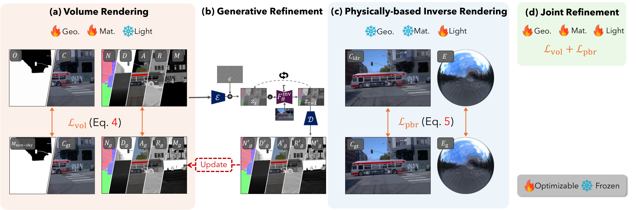
Inverse rendering recovers the scene geometry, material, and lighting (Sec . ) from the input video. However, recovering all scene properties jointly is highly ill-posed. Therefore, we adopt a multi-stage framework that optimizes one sub-problem at a time (Fig. ): (a) a volume rendering stage reconstructs geometry and material under generative G-buffer priors; (b) a generative refinement step sharpens those intrinsics while enforcing multi-view consistency, and stages (a)(b) alternate to progressively clean the supervision; (c) a physically-based inverse rendering stage solves for lighting; and (d) a final stage jointly refines all parameters. We argue that the order matters: lighting can be disentangled only once geometry and material are reliable. We describe each stage in detail below.

Volume Rendering Stage.

This stage optimizes all Gaussian attributes, recovering geometry and material. First, We initialize the Gaussian positions $\{\boldsymbol{\mu}\}$ from unprojected LiDAR points [12], run the volume rendering pass each iteration, and minimize

\mathcal{L}_{\text{vol}}=\mathcal{L}_{\text{rgb}}+\lambda_{O}\mathcal{L}_{O}+\lambda_{D}\mathcal{L}_{D}+\lambda_{N}\mathcal{L}_{N}+\lambda_{A}\mathcal{L}_{A}+\lambda_{R}\mathcal{L}_{R}+\lambda_{M}\mathcal{L}_{M}.

(4)

The photometric loss $\mathcal{L}_{\text{rgb}}=\|\mathbf{C}-\mathbf{C}_{\text{gt}}\|+\text{SSIM}(\mathbf{C},\mathbf{C}_{\text{gt}})$ supervises appearance. Although $\mathbf{C}$ is not the final render, fitting it reconstructs accurate geometry. An opacity term $\mathcal{L}_{O}=\text{B.C.E}(\mathbf{O},\mathbf{M}_{\text{non-sky}})$ aligns opacity and non-sky mask from SegFormer [79] with binary cross-entropy, suppressing sky floaters that would cast spurious shadows. The remaining terms regularize the geometry and material toward the generative prior [45], which is essential for alleviating the inverse-rendering ambiguity. The inverse model $\mathbf{F}_{\theta}$ generates G-buffers $\{\mathbf{N}_{g},\mathbf{D}_{g},\mathbf{A}_{g},\mathbf{R}_{g},\mathbf{M}_{g}\}$ from the input frames. Because a full sequence exceeds the model’s frame limit, we split it into overlapping clips and blend the outputs using sliding-window averaging. These priors regularize depth: $\mathcal{L}_{D}=\|\mathbf{D}-\mathbf{D}_{\text{lidar}}\|+\|(u\mathbf{D}+v)-\mathbf{D}_{g}\|$ , with $u,v$ aligning scale & shift [87], normals: $\mathcal{L}_{N}=\|\mathbf{N}-\mathbf{N}_{g}\|-\mathbf{N}\cdot\mathbf{N}_{g}$ , and materials: $\mathcal{L}_{A}=\|\mathbf{A}-\mathbf{A}_{g}\|$ , $\mathcal{L}_{R}=\|\mathbf{R}-\mathbf{R}_{g}\|$ , $\mathcal{L}_{M}=\|\mathbf{M}-\mathbf{M}_{g}\|$ .

Generative Refinement Stage.

Sliding-window averaging reduces, but does not eliminate, the temporal inconsistency of the per-frame G-buffer priors $\{\mathbf{X}_{g}\}$ (where $\mathbf{X}\in\{\mathbf{N},\mathbf{D},\mathbf{A},\mathbf{R},\mathbf{M}\}$ ). The residual inconsistency feeds contradictory supervision signals into Eq. , producing floaters and blurry reconstructions. We resolve this with the same SDEdit operator used in forward rendering (Eq. ), but now applied to intrinsics at training time rather than RGB at inference time, which is the key distinction between the two generative steps. After the volume rendering stage converges, we render each intrinsic map $\mathbf{X}$ from the 3D representation: these renders are multi-view consistent but blurrier than the raw priors $\mathbf{X}_{g}$ . We use them as structural anchors and refine them with the video diffusion [45] inverse model $\mathbf{F}_{\theta}$ by $\mathbf{X}_{g}=\textsc{SDEdit}(\mathbf{X}_{g}\mid\mathbf{F}_{\theta},\mathcal{E}(\mathbf{C}_{\text{gt}}),\tau)$ . Hence, the refined intrinsic maps $\mathbf{X}_{g}$ are sharp and temporally consistent. We update $\{\mathbf{X}_{g}\}$ as supervision in the next round of the volume rendering stage, enhancing reconstruction quality.

Physically-based Inverse Rendering Stage.

With geometry and material reconstructed, we solve for lighting. Lighting cannot be supervised directly under the heavy occlusion of driving sequences, but it can be recovered by matching shading: we freeze geometry and material, render with the PBR pass (Eq. ), and minimize:

\mathcal{L}_{\text{pbr}}=\|\mathbf{C}_{\text{ldr}}-\mathbf{C}_{\text{gt}}\|+\lambda_{E}\mathcal{L}_{E},\hskip 9.24994pt\mathcal{L}_{E}=\sum_{\boldsymbol{\omega}}\|\log\mathbf{E}(\boldsymbol{\omega})-\log\mathbf{E}_{g}(\boldsymbol{\omega})\|.

(5)

The photometric term aligns the PBR rendering with the input frames. The lighting loss $\mathcal{L}_{E}$ regularizes $\mathbf{E}$ toward the generative prior $\mathbf{E}_{g}$ , the HDR environment maps predicted by DiffusionLight [58, 13] and averaged over views. We compute this term in log space because the lighting is high dynamic range, which stabilizes the loss. Finally, a joint refinement stage optimizes geometry, material, and lighting together with loss $\mathcal{L}_{\text{vol}}+\mathcal{L}_{\text{pbr}}$ , maximizing overall quality.

4 Experiments

4.1 Evaluation Settings

Datasets.

We evaluate our method on real-world and synthetic datasets. For real-world evaluation, we use scenes from the Waymo Open Dataset (WOD) [70], featuring diverse lighting and driving dynamics. From each scene, we select 50 consecutive single-camera frames, reserving every 10th frame for testing and the remainder for training or conditioning.

Because capturing ground-truth materials and relighting videos are difficult, we simulate 6 synthetic urban scenes. Specifically, we composite city assets [6] with HDR environment maps [59] and render RGB and PBR material maps using Blender Cycles [14]. Each scene features two parallel camera trajectories, providing 46 training frames and 51 testing frames. To evaluate under diverse illuminations (sunny, cloudy, sunset), we render each scene with 4 environment maps: one for training and three for relighting evaluation. This enables a comprehensive quantitative assessment of inverse rendering, view synthesis, and relighting.

Baselines.

We compare our method against physically-based inverse rendering methods, including UrbanIR [50] and InvRGB+L [9]. UrbanIR represents geometry and base color as neural fields and renders videos using sun-sky lighting. InvRGB+L embeds scene properties in 3D Gaussian attributes and leverages LiDAR reflectance model for robust material estimation. Additionally, to compare against pure generative models in our target task, we construct a baseline that uses Gen3C [61] for view synthesis and DiffusionRenderer (DR) [45] for inverse rendering and relighting. We refer to this baseline as Gen3C+DR. The official implementation is used throughout the evaluation.

Metrics.

For view synthesis and relighting, the metric is calculated with PSNR, SSIM [74], and LPIPS [94]. For inverse rendering, roughness and metallic are evaluated using root-mean-square error (RMSE), and the normal is evaluated using mean angular error (MAE). For albedo, we follow [45] to estimate a three-channel scaling factor via least-squares minimization and apply the scaling before calculating PSNR, referred to as si-PSNR.

4.2 Qualitative Evaluation

Forward Rendering.

Figure compares our novel view synthesis and relighting results against baselines on real-world WOD scenes. First of all, we synthesize novel view and relight the dynamic scene with a new lighting condition (e.g., sunset). To ensure a fair comparison, we converted the environment map into the representations required by UrbanIR [50] and InvRGB+L [9] (full details of both procedures are provided in the supplementary material). In this evaluation, UrbanIR [50] is limited to static scene, and reconstructs poorly for dynamic objects. InvRGB+L [9] suffers from imperfect reconstruction of physical models and produces severe artifacts that degrade the relighting quality. In contrast, BRDFusion follows the lighting and produces realistic shading.

Additionally, we simulate starry night scenes with local light sources, such as streetlights and car headlights. We set the positions and directions of local lights in 3D and render using importance sampling. Please refer to the supplementary material for more details. Physically-based methods like UrbanIR [50] and InvRGB+L [9] can simulate these effects, but they suffer from shadow baking, geometry artifacts exposed by local lighting. On the other hand, the generative approach Gen3C [61]+DR [45] fails to simulate local lights because it lacks an explicit 3D representation. The generation process cannot be precisely controlled, and the output cannot follow the target lighting while modifying scene structures (e.g., trees). In contrast, our method leverages both physically based and generative models for inverse and forward rendering, achieving high-quality rendering and precise lighting control, outperforming baselines significantly.

Inverse Rendering.

Figure compares our inverse rendering performance against the baselines in novel viewpoints from a dynamic WOD scene. UrbanIR [50] fails to reconstruct the dynamic scenes, while InvRGB+L [9] predicts incorrect material (e.g., white cars with dark albedo) and produces overly smooth G-buffers without scene details, degrading rendering quality for downstream applications (Fig. ). Although the Gen3C [61] + DR [45] baseline produces highly detailed outputs, its inherent randomness cannot guarantee physically plausible and consistent predictions. In contrast, BRDFusion integrates generative modeling into physically-based optimization, yielding detailed, physically-plausible, and view- and temporally-consistent geometry and material.

Table 1: Quantitative comparison on synthetic data. The best, second best, and the third result is marked as red, orange, and yellow.

	Inverse Rendering				Novel View Synthesis			Novel View Relighting
Method	Albedo (si-PSNR $\uparrow$ )	Roughness (RMSE $\downarrow$ )	Metallic (RMSE $\downarrow$ )	Normal (MAE $\downarrow$ )	PSNR $\uparrow$	SSIM $\uparrow$	LPIPS $\downarrow$	PSNR $\uparrow$	SSIM $\uparrow$	LPIPS $\downarrow$
UrbanIR [50]	16.55	-	-	26.21	20.97	0.677	0.258	15.61	0.586	0.415
InvRGB+L [9]	18.17	0.329	-	17.67	20.62	0.673	0.352	14.55	0.544	0.482
Gen3C [61]+DR [45]	19.33	0.206	0.321	21.93	22.74	0.710	0.293	16.49	0.599	0.415
Ours	18.99	0.187	0.174	17.11	21.83	0.670	0.390	18.33	0.604	0.448

4.3 Quantitative Evaluation

Table reports the quantitative comparison for inverse rendering, novel view synthesis, and relighting on the synthetic dataset. We compute inverse rendering metrics only over non-sky regions to avoid ambiguity in sky material definition. For inverse rendering, we achieve the highest accuracy in roughness, metallic, and normal estimation, with albedo estimation comparable to the Gen3C [61]+DR [45] baseline. BRDFusion only achieves a comparable metric for novel-view synthesis, at the cost of clean decomposition. However, it performs significantly better at novel-view relighting. Specifically, we achieve the highest PSNR, SSIM, and comparable LPIPS scores across all baselines, demonstrating our ability to faithfully simulate diverse lighting effects. This highlights the benefits of reconstructing high-quality 3D geometry and material, and integration of generative models.

4.4 Ablation Study

To validate the design choices, we conduct an ablation study on a scene from our synthetic dataset. To better demonstrate the effectiveness of our full pipeline, we adopt a more comprehensive setting than qualitative comparison: 3 synchronized cameras, 273 training frames, and 300 testing frames. Quantitative results are presented in Tab. . Additional ablations and qualitative visualizations are provided in the supplementary material due to space constraints.

We ablate the following configurations: No PBR Optim.: The variant bypasses PBR optimization and relies solely on the Volume Rendering with generative models [45, 58, 13]. While the generative models provide roughly correct initial estimates, they are not view- and temporally-consistent, leading to artifacts during optimization. Therefore, PBR optimization is essential for accurately disentangling materials, geometry, and lighting to achieve optimal inverse rendering and relighting. No Gen. Optim.: The variant performs physically-based inverse rendering without the generative prior during the optimization. The highly ill-posed nature of inverse rendering makes the model fail catastrophically. Without proper regularization, the model bakes lighting effects, such as shadows, directly into the geometry or material representations. While this yields high-quality novel view synthesis, the method cannot accurately estimate meaningful scene decomposition (e.g., 110.8 for normal MAE), thereby degrading novel view relighting performance. No Gen. Render: Finally, bypassing the generative rendering stage negatively impacts the final output quality. The generative rendering stage effectively alleviates artifacts of Monte Carlo integration and imperfect reconstruction, resulting in improved metrics for view synthesis and relighting. As reported in Tab. , the full pipeline elegantly integrates physically-based and generative models, achieving the best overall performance.

Table 2: Ablation study on our synthetic dataset. The best, second best, and the third result is marked as red, orange, and yellow. Inverse rendering metrics for the "No Gen. Render" baseline are identical to our full method, as generative rendering is only applied for view synthesis and relighting.

	Inverse Rendering				Novel View Synthesis			Novel View Relighting
Method	Albedo (si-PSNR $\uparrow$ )	Roughness (RMSE $\downarrow$ )	Metallic (RMSE $\downarrow$ )	Normal (MAE $\downarrow$ )	PSNR $\uparrow$	SSIM $\uparrow$	LPIPS $\downarrow$	PSNR $\uparrow$	SSIM $\uparrow$	LPIPS $\downarrow$
No PBR Optim.	18.64	0.200	0.230	17.17	13.58	0.525	0.511	18.41	0.590	0.473
No Gen. Optim.	15.72	0.248	0.724	110.8	22.93	0.690	0.366	14.83	0.523	0.519
No Gen. Render	18.72	0.199	0.233	16.88	19.88	0.619	0.375	18.64	0.597	0.406
Ours (Full Method)	18.72	0.199	0.233	16.88	20.54	0.646	0.417	18.83	0.608	0.450

4.5 Implementation Details

Our method is built upon OmniRe [11] and 3DGRT [55]. Our pipeline executes sequentially: an initial Volume Rendering stage for 30,000 iterations, Generative Refinement, a second Volume Rendering pass for 30,000 iterations, Physically-based Inverse Rendering for 5,000 iterations, and a final joint optimization stage for 20,000 iterations. We set the learning rate to $1\times 10$ . All experiments are conducted on a single NVIDIA RTX A6000 GPU. During training, we trace $N_{r}=512$ rays and sample 2048 pixels per iteration [24] to accelerate the process. $N_{r}=256$ rays are used for testing. Total training takes approximately 10-11 hours. Detailed hyperparameters and runtime breakdowns are provided in the supplementary material.

4.6 Diverse Applications

By decomposing the scene into its underlying geometry, material, and lighting components, our method enables a diverse range of downstream applications, as illustrated in Fig. . We perform relighting using publicly available environment maps [88] to simulate varying conditions, such as sunset or nighttime scenarios (Fig. (b), (c)). Beyond lighting changes, our explicit 3D representation supports realistic object insertion with consistent secondary lighting effects, such as cast shadows (Fig. (d)); this is achieved by seamlessly integrating a reconstructed object from another scene into the target environment. Furthermore, we can introduce localized illumination, such as headlights or streetlights, by placing point or spot lights within the reconstructed 3D scene (Fig. (e)). These capabilities demonstrate the potential of our representation for high-fidelity scene manipulation and for generating physically consistent synthetic data for various vision tasks, such as simulation for autonomous driving systems.

5 Conclusion

We present BRDFusion, a novel framework for inverse rendering in dynamic urban scenes. By integrating physically-based inverse rendering with a generative refinement process, our approach successfully bridges the high controllability of PBR methods with the photorealism of generative models. This hybrid rendering pipeline enables a variety of downstream tasks, including novel view relighting, object insertion, and nighttime simulation.

Limitations.

First, while our method supports inserting virtual local lights, the inverse rendering pipeline does not explicitly model emissive materials. Consequently, decomposing nighttime sequences with active headlights or streetlights remains challenging. Second, like other 3D reconstruction methods, floaters may appear in unobserved regions. Finally, while our refinement mitigates minor inconsistencies, catastrophic failures of generative models can still cause incorrect scene decomposition. We detail failure cases in the supplementary material and leave them for future work.

Acknowledgements

This research was funded by the National Science and Technology Council, Taiwan, under Grants NSTC 112-2222-E-A49-004-MY2 and 113-2628-E-A49-023-. The authors are grateful to Google, NVIDIA, and MediaTek Inc. for their generous donations. Yu-Lun Liu acknowledges the Yushan Young Fellow Program by the MOE in Taiwan.

References

[1] Bai, H., Zhu, J., Jiang, S., Huang, W., Lu, T., Li, Y., Guo, J., Fu, R., Guo, Y., Chen, L.: Gare: Relightable 3d gaussian splatting for outdoor scenes from unconstrained photo collections. arXiv preprint arXiv:2507.20512 (2025)
[2] Barron, J.T., Malik, J.: Shape, illumination, and reflectance from shading. IEEE transactions on pattern analysis and machine intelligence 37(8), 1670–1687 (2014)
[3] Barrow, H., Tenenbaum, J., Hanson, A., Riseman, E.: Recovering intrinsic scene characteristics. Comput. vis. syst 2(3-26), 2 (1978)
[4] Beißwenger, O., Dihlmann, J.N., Lensch, H.P.: Framediffuser: G-buffer-conditioned diffusion for neural forward frame rendering. arXiv preprint (2025)
[5] Bell, S., Bala, K., Snavely, N.: Intrinsic images in the wild. ACM Transactions on Graphics (TOG) (2014)
[6] BlenderKit Community: Blenderkit – free 3d assets for blender. https://www.blenderkit.com (2025), accessed: 2025-08-14
[7] Chen, H., Lin, Z., Zhang, J.: Gi-gs: Global illumination decomposition on gaussian splatting for inverse rendering. arXiv preprint arXiv:2410.02619 (2024)
[8] Chen, X., Peng, S., Yang, D., Liu, Y., Pan, B., Lv, C., Zhou, X.: Intrinsicanything: Learning diffusion priors for inverse rendering under unknown illumination. In: European Conference on Computer Vision. pp. 450–467. Springer (2024)
[9] Chen, X., Chandaka, B., Lin, C.H., Zhang, Y.Q., Forsyth, D., Zhao, H., Wang, S.: Invrgb+l: Inverse rendering of complex scenes with unified color and lidar reflectance modeling. In: ICCV (2025)
[10] Chen, Z., Xu, T., Ge, W., Wu, L., Yan, D., He, J., Wang, L., Zeng, L., Zhang, S., Chen, Y.C.: Uni-renderer: Unifying rendering and inverse rendering via dual stream diffusion. In: Proceedings of the Computer Vision and Pattern Recognition Conference. pp. 26504–26513 (2025)
[11] Chen, Z., Yang, J., Huang, J., De Lutio, R., Esturo, J.M., Ivanovic, B., Litany, O., Gojcic, Z., Fidler, S., Pavone, M., et al.: Omnire: Omni urban scene reconstruction. arXiv preprint arXiv:2408.16760 (2024)
[12] Chen, Z., Yang, J., Huang, J., de Lutio, R., Esturo, J.M., Ivanovic, B., Litany, O., Gojcic, Z., Fidler, S., Pavone, M., Song, L., Wang, Y.: Omnire: Omni urban scene reconstruction. In: ICLR (2025)
[13] Chinchuthakun, W., Phongthawee, P., Raj, A., Jampani, V., Khungurn, P., Suwajanakorn, S.: Diffusionlight-turbo: Accelerated light probes for free via single-pass chrome ball inpainting. IEEE Transactions on Pattern Analysis and Machine Intelligence (2026)
[14] Community, B.O.: Blender - a 3D modelling and rendering package. Blender Foundation, Stichting Blender Foundation, Amsterdam (2018), http://www.blender.org
[15] Cook, R.L., Porter, T., Carpenter, L.: Distributed ray tracing. In: Proceedings of the 11th annual conference on Computer graphics and interactive techniques (1984)
[16] Cook, R.L., Torrance, K.E.: A reflectance model for computer graphics. ACM Transactions on Graphics (ToG) (1982)
[17] Fu, X., Yin, W., Hu, M., Wang, K., Ma, Y., Tan, P., Shen, S., Lin, D., Long, X.: Geowizard: Unleashing the diffusion priors for 3d geometry estimation from a single image. In: European Conference on Computer Vision. pp. 241–258. Springer (2024)
[18] Gao, J., Gu, C., Lin, Y., Li, Z., Zhu, H., Cao, X., Zhang, L., Yao, Y.: Relightable 3d gaussians: Realistic point cloud relighting with brdf decomposition and ray tracing. In: European Conference on Computer Vision. pp. 73–89. Springer (2024)
[19] Gardner, J., Egger, B., Smith, W.: Rotation-equivariant conditional spherical neural fields for learning a natural illumination prior. Advances in Neural Information Processing Systems 35, 26309–26323 (2022)
[20] Gardner, J.A., Kashin, E., Egger, B., Smith, W.A.: The sky’s the limit: Relightable outdoor scenes via a sky-pixel constrained illumination prior and outside-in visibility. In: European conference on computer vision. pp. 126–143. Springer (2024)
[21] Griffiths, D., Ritschel, T., Philip, J.: Outcast: Outdoor single-image relighting with cast shadows. Computer Graphics Forum 41(2), 179–193 (2022)
[22] Grosse, R., Johnson, M.K., Adelson, E.H., Freeman, W.T.: Ground truth dataset and baseline evaluations for intrinsic image algorithms. In: 2009 IEEE 12th International Conference on Computer Vision. pp. 2335–2342. Ieee (2009)
[23] Gu, C., Wei, X., Zeng, Z., Yao, Y., Zhang, L.: Irgs: Inter-reflective gaussian splatting with 2d gaussian ray tracing. In: Proceedings of the Computer Vision and Pattern Recognition Conference. pp. 10943–10952 (2025)
[24] Gu, C., Wei, X., Zeng, Z., Yao, Y., Zhang, L.: Irgs: Inter-reflective gaussian splatting with 2d gaussian ray tracing. In: CVPR (2025)
[25] Hasselgren, J., Hofmann, N., Munkberg, J.: Shape, light, and material decomposition from images using monte carlo rendering and denoising. Advances in Neural Information Processing Systems 35, 22856–22869 (2022)
[26] He, J., Li, H., Yin, W., Liang, Y., Li, L., Zhou, K., Zhang, H., Liu, B., Chen, Y.C.: Lotus: Diffusion-based visual foundation model for high-quality dense prediction. arXiv preprint arXiv:2409.18124 (2024)
[27] He, K., Liang, R., Munkberg, J., Hasselgren, J., Vijaykumar, N., Keller, A., Fidler, S., Gilitschenski, I., Gojcic, Z., Wang, Z.: Unirelight: Learning joint decomposition and synthesis for video relighting. NeurIPS (2025)
[28] He, Z., Wang, T., Huang, X., Pan, X., Liu, Z.: Neural lightrig: Unlocking accurate object normal and material estimation with multi-light diffusion. In: Proceedings of the Computer Vision and Pattern Recognition Conference. pp. 26514–26524 (2025)
[29] Hold-Geoffroy, Y., Athawale, A., Lalonde, J.F.: Deep sky modeling for single image outdoor lighting estimation. In: Proceedings of the IEEE/CVF conference on computer vision and pattern recognition. pp. 6927–6935 (2019)
[30] Hold-Geoffroy, Y., Sunkavalli, K., Hadap, S., Gambaretto, E., Lalonde, J.F.: Deep outdoor illumination estimation. In: Proceedings of the IEEE conference on computer vision and pattern recognition. pp. 7312–7321 (2017)
[31] Huang, X., Wang, T., Liu, Z., Wang, Q.: Material anything: Generating materials for any 3d object via diffusion. In: Proceedings of the Computer Vision and Pattern Recognition Conference. pp. 26556–26565 (2025)
[32] Jiang, Y., Tu, J., Liu, Y., Gao, X., Long, X., Wang, W., Ma, Y.: Gaussianshader: 3d gaussian splatting with shading functions for reflective surfaces. In: Proceedings of the IEEE/CVF conference on computer vision and pattern recognition. pp. 5322–5332 (2024)
[33] Jin, H., Li, Y., Luan, F., Xiangli, Y., Bi, S., Zhang, K., Xu, Z., Sun, J., Snavely, N.: Neural gaffer: Relighting any object via diffusion. Advances in Neural Information Processing Systems 37, 141129–141152 (2024)
[34] Jin, H., Liu, I., Xu, P., Zhang, X., Han, S., Bi, S., Zhou, X., Xu, Z., Su, H.: Tensoir: Tensorial inverse rendering. In: Proceedings of the IEEE/CVF Conference on Computer Vision and Pattern Recognition. pp. 165–174 (2023)
[35] Kajiya, J.T.: The rendering equation. In: Proceedings of the 13th Annual Conference on Computer Graphics and Interactive Techniques (1986)
[36] Kaleta, J., Kania, K., Trzcinski, T., Kowalski, M.: Lumigauss: relightable gaussian splatting in the wild. In: Proceedings of the Winter Conference on Applications of Computer Vision. pp. 1–10 (2025)
[37] Karis, B.: Real shading in Unreal Engine 4. ACM SIGGRAPH Course on Physically Based Shading Theory and Practice (2013)
[38] Karras, T., Aittala, M., Aila, T., Laine, S.: Elucidating the design space of diffusion-based generative models. In: Proc. NeurIPS (2022)
[39] Ke, B., Obukhov, A., Huang, S., Metzger, N., Daudt, R.C., Schindler, K.: Repurposing diffusion-based image generators for monocular depth estimation. In: Proceedings of the IEEE/CVF conference on computer vision and pattern recognition. pp. 9492–9502 (2024)
[40] Kerbl, B., Kopanas, G., Leimkühler, T., Drettakis, G.: 3d gaussian splatting for real-time radiance field rendering. ACM Trans. Graph. (2023)
[41] Kocsis, P., Sitzmann, V., Nießner, M.: Intrinsic image diffusion for indoor single-view material estimation. In: Proceedings of the IEEE/CVF Conference on Computer Vision and Pattern Recognition. pp. 5198–5208 (2024)
[42] Li, Q., Guo, J., Fei, Y., Li, F., Guo, Y.: Neulighting: Neural lighting for free viewpoint outdoor scene relighting with unconstrained photo collections. In: SIGGRAPH Asia 2022 Conference Papers. pp. 1–9 (2022)
[43] Li, Z., Shafiei, M., Ramamoorthi, R., Sunkavalli, K., Chandraker, M.: Inverse rendering for complex indoor scenes: Shape, spatially-varying lighting and svbrdf from a single image. In: CVPR (2020)
[44] Li, Z., Wu, T., Tan, J., Zhang, M., Wang, J., Lin, D.: Idarb: Intrinsic decomposition for arbitrary number of input views and illuminations. arXiv preprint arXiv:2412.12083 (2024)
[45] Liang, R., Gojcic, Z., Ling, H., Munkberg, J., Hasselgren, J., Lin, Z.H., Gao, J., Keller, A., Vijaykumar, N., Fidler, S., Wang, Z.: Diffusionrenderer: Neural inverse and forward rendering with video diffusion models. In: CVPR (2025)
[46] Liang, R., Gojcic, Z., Nimier-David, M., Acuna, D., Vijaykumar, N., Fidler, S., Wang, Z.: Photorealistic object insertion with diffusion-guided inverse rendering. In: European Conference on Computer Vision. pp. 446–465. Springer (2024)
[47] Liang, R., He, K., Gojcic, Z., Gilitschenski, I., Fidler, S., Vijaykumar, N., Wang, Z.: Luxdit: Lighting estimation with video diffusion transformer. NeurIPS (2026)
[48] Liang, Z., Zhang, Q., Feng, Y., Shan, Y., Jia, K.: Gs-ir: 3d gaussian splatting for inverse rendering. arXiv preprint arXiv:2311.16473 (2023)
[49] Liao, L., Zhang, C., Wu, T., Lv, H., Deng, B., Gao, L.: Rosgs: Relightable outdoor scenes with gaussian splatting. arXiv preprint arXiv:2509.11275 (2025)
[50] Lin, C.H., Liu, B., Chen, Y.T., Chen, K.S., Forsyth, D., Huang, J.B., Bhattad, A., Wang, S.: Urbanir: Large-scale urban scene inverse rendering from a single video. In: 2025 International Conference on 3D Vision (3DV). pp. 512–523. IEEE (2025)
[51] Litman, Y., Patashnik, O., Deng, K., Agrawal, A., Zawar, R., De la Torre, F., Tulsiani, S.: Materialfusion: Enhancing inverse rendering with material diffusion priors. In: 2025 International Conference on 3D Vision (3DV). pp. 802–812. IEEE (2025)
[52] Lyu, L., Tewari, A., Habermann, M., Saito, S., Zollhöfer, M., Leimkühler, T., Theobalt, C.: Diffusion posterior illumination for ambiguity-aware inverse rendering. ACM Transactions on Graphics (TOG) 42(6), 1–14 (2023)
[53] Meng, C., He, Y., Song, Y., Song, J., Wu, J., Zhu, J.Y., Ermon, S.: SDEdit: Guided image synthesis and editing with stochastic differential equations. In: International Conference on Learning Representations (2022)
[54] Mildenhall, B., Srinivasan, P.P., Tancik, M., Barron, J.T., Ramamoorthi, R., Ng, R.: NeRF: representing scenes as neural radiance fields for view synthesis. arXiv preprint arXiv:2003.08934 (2020)
[55] Moenne-Loccoz, N., Mirzaei, A., Perel, O., de Lutio, R., Esturo, J.M., State, G., Fidler, S., Sharp, N., Gojcic, Z.: 3d gaussian ray tracing: Fast tracing of particle scenes. ACM Transactions on Graphics and SIGGRAPH Asia (2024)
[56] Munkberg, J., Hasselgren, J., Shen, T., Gao, J., Chen, W., Evans, A., Müller, T., Fidler, S.: Extracting triangular 3d models, materials, and lighting from images. In: Proceedings of the IEEE/CVF conference on computer vision and pattern recognition. pp. 8280–8290 (2022)
[57] Philip, J., Gharbi, M., Zhou, T., Efros, A.A., Drettakis, G.: Multi-view relighting using a geometry-aware network. ACM Transactions on Graphics (TOG) (2019)
[58] Phongthawee, P., Chinchuthakun, W., Sinsunthithet, N., Jampani, V., Raj, A., Khungurn, P., Suwajanakorn, S.: Diffusionlight: Light probes for free by painting a chrome ball. In: Proceedings of the IEEE/CVF conference on computer vision and pattern recognition. pp. 98–108 (2024)
[59] Poly Haven: Poly haven: The public asset library. Online Resource (2024), https://polyhaven.com/, accessed: 2024-03-01
[60] Pun, A., Sun, G., Wang, J., Chen, Y., Yang, Z., Manivasagam, S., Ma, W.C., Urtasun, R.: Lightsim: Neural lighting simulation for urban scenes. arXiv preprint arXiv:2312.06654 (2023)
[61] Ren, X., Shen, T., Huang, J., Ling, H., Lu, Y., Nimier-David, M., Müller, T., Keller, A., Fidler, S., Gao, J.: Gen3c: 3d-informed world-consistent video generation with precise camera control. In: CVPR (2025)
[62] Rombach, R., Blattmann, A., Lorenz, D., Esser, P., Ommer, B.: High-resolution image synthesis with latent diffusion models. In: Proceedings of the IEEE/CVF conference on computer vision and pattern recognition. pp. 10684–10695 (2022)
[63] Rudnev, V., Elgharib, M., Smith, W., Liu, L., Golyanik, V., Theobalt, C.: Nerf for outdoor scene relighting. In: European Conference on Computer Vision. pp. 615–631. Springer (2022)
[64] Rudnev, V., Elgharib, M., Smith, W., Liu, L., Golyanik, V., Theobalt, C.: NeRF for outdoor scene relighting. In: ECCV (2022)
[65] Sartor, S., Peers, P.: Matfusion: a generative diffusion model for svbrdf capture. In: SIGGRAPH Asia 2023 conference papers. pp. 1–10 (2023)
[66] Schlick, C.: An inexpensive brdf model for physically-based rendering. Computer Graphics Forum 13(3), 233–246 (1994)
[67] Srinivasan, P.P., Deng, B., Zhang, X., Tancik, M., Mildenhall, B., Barron, J.T.: Nerv: Neural reflectance and visibility fields for relighting and view synthesis. In: CVPR (2021)
[68] Sun, H., Gao, Y., Xie, J., Yang, J., Wang, B.: Svg-ir: Spatially-varying gaussian splatting for inverse rendering. In: Proceedings of the Computer Vision and Pattern Recognition Conference. pp. 16143–16152 (2025)
[69] Sun, J.M., Wu, T., Yang, Y.L., Lai, Y.K., Gao, L.: Sol-nerf: Sunlight modeling for outdoor scene decomposition and relighting. In: SIGGRAPH Asia 2023 Conference Papers. pp. 1–11 (2023)
[70] Sun, P., Kretzschmar, H., Dotiwalla, X., Chouard, A., Patnaik, V., Tsui, P., Guo, J., Zhou, Y., Chai, Y., Caine, B., et al.: Scalability in perception for autonomous driving: Waymo open dataset. In: CVPR (2020)
[71] Veach, E., Guibas, L.J.: Optimally combining sampling techniques for monte carlo rendering. In: Proceedings of the 22nd annual conference on Computer graphics and interactive techniques (1995)
[72] Walter, B., Marschner, S.R., Li, H., Torrance, K.E.: Microfacet models for refraction through rough surfaces. In: Proceedings of the 18th Eurographics Conference on Rendering Techniques. p. 195–206. EGSR’07, Eurographics Association, Goslar, DEU (2007)
[73] Wang, J., Hu, Q., Bao, C., Zhu, Y., Bao, H., Cui, Z., Zhang, G.: Lightcity: An urban dataset for outdoor inverse rendering and reconstruction under multi-illumination conditions. In: Proceedings of the IEEE/CVF International Conference on Computer Vision. pp. 26477–26487 (2025)
[74] Wang, Z., Bovik, A.C., Sheikh, H.R., Simoncelli, E.P.: Image quality assessment: from error visibility to structural similarity. IEEE transactions on image processing (2004)
[75] Wang, Z., Chen, W., Acuna, D., Kautz, J., Fidler, S.: Neural light field estimation for street scenes with differentiable virtual object insertion. In: European Conference on Computer Vision. pp. 380–397. Springer (2022)
[76] Wang, Z., Shen, T., Gao, J., Huang, S., Munkberg, J., Hasselgren, J., Gojcic, Z., Chen, W., Fidler, S.: Neural fields meet explicit geometric representations for inverse rendering of urban scenes. In: Proceedings of the IEEE/CVF Conference on Computer Vision and Pattern Recognition. pp. 8370–8380 (2023)
[77] Wu, S., Basu, S., Broedermann, T., Van Gool, L., Sakaridis, C.: Pbr-nerf: Inverse rendering with physics-based neural fields. In: Proceedings of the Computer Vision and Pattern Recognition Conference. pp. 10974–10984 (2025)
[78] Wu, Z., Chen, J., Li, L., Wu, S., Zhu, Z., Xu, K., Oswald, M.R., Song, J.: 3d gaussian inverse rendering with approximated global illumination. arXiv preprint arXiv:2504.01358 (2025)
[79] Xie, E., Wang, W., Yu, Z., Anandkumar, A., Alvarez, J.M., Luo, P.: Segformer: Simple and efficient design for semantic segmentation with transformers. In: Advances in Neural Information Processing Systems (2021)
[80] Yang, S., Cui, X., Zhu, Y., Tang, J., Li, S., Yu, Z., Shi, B.: Complementary intrinsics from neural radiance fields and cnns for outdoor scene relighting. In: Proceedings of the IEEE/CVF conference on computer vision and pattern recognition. pp. 16600–16609 (2023)
[81] Yao, Y., Zhang, J., Liu, J., Qu, Y., Fang, T., McKinnon, D., Tsin, Y., Quan, L.: Neilf: Neural incident light field for physically-based material estimation. In: ECCV (2022)
[82] Ye, C., Qiu, L., Gu, X., Zuo, Q., Wu, Y., Dong, Z., Bo, L., Xiu, Y., Han, X.: Stablenormal: Reducing diffusion variance for stable and sharp normal. ACM Transactions on Graphics (ToG) 43(6), 1–18 (2024)
[83] Ye, K., Hou, Q., Zhou, K.: 3d gaussian splatting with deferred reflection. In: ACM SIGGRAPH 2024 Conference Papers. pp. 1–10 (2024)
[84] Ye, K., Hou, Q., Zhou, K.: Progressive radiance distillation for inverse rendering with gaussian splatting. arXiv preprint arXiv:2408.07595 (2024)
[85] Yu, Y., Meka, A., Elgharib, M., Seidel, H.P., Theobalt, C., Smith, W.A.: Self-supervised outdoor scene relighting. In: European Conference on Computer Vision. pp. 84–101. Springer (2020)
[86] Yu, Y., Smith, W.A.: Inverserendernet: Learning single image inverse rendering. In: Proceedings of the IEEE/CVF Conference on Computer Vision and Pattern Recognition. pp. 3155–3164 (2019)
[87] Yu, Z., Peng, S., Niemeyer, M., Sattler, T., Geiger, A.: Monosdf: Exploring monocular geometric cues for neural implicit surface reconstruction. in arXiv (2022)
[88] Zaal, G., et al.: Poly Haven - The Public 3D Asset Library (2024), https://polyhaven.com
[89] Zeng, C., Dong, Y., Peers, P., Kong, Y., Wu, H., Tong, X.: Dilightnet: Fine-grained lighting control for diffusion-based image generation. In: ACM SIGGRAPH 2024 Conference Papers. pp. 1–12 (2024)
[90] Zeng, Z., Deschaintre, V., Georgiev, I., Hold-Geoffroy, Y., Hu, Y., Luan, F., Yan, L.Q., Hašan, M.: RGB $\leftrightarrow$ X: image decomposition and synthesis using material-and lighting-aware diffusion models. In: ACM SIGGRAPH 2024 Conference Papers (2024)
[91] Zhang, J., Yao, Y., Li, S., Liu, J., Fang, T., McKinnon, D., Tsin, Y., Quan, L.: Neilf++: Inter-reflectable light fields for geometry and material estimation. In: Proceedings of the IEEE/CVF International Conference on Computer Vision. pp. 3601–3610 (2023)
[92] Zhang, K., Luan, F., Wang, Q., Bala, K., Snavely, N.: PhySG: Inverse rendering with spherical Gaussians for physics-based material editing and relighting. In: CVPR (2021)
[93] Zhang, L., Rao, A., Agrawala, M.: Scaling in-the-wild training for diffusion-based illumination harmonization and editing by imposing consistent light transport. In: The Thirteenth International Conference on Learning Representations (2025)
[94] Zhang, R., Isola, P., Efros, A.A., Shechtman, E., Wang, O.: The unreasonable effectiveness of deep features as a perceptual metric. In: Proceedings of the IEEE conference on computer vision and pattern recognition (2018)
[95] Zhang, X., Gao, W., Jain, S., Maire, M., Forsyth, D., Bhattad, A.: Latent intrinsics emerge from training to relight. Advances in Neural Information Processing Systems 37, 96775–96796 (2024)
[96] Zhang, X., Srinivasan, P.P., Deng, B., Debevec, P., Freeman, W.T., Barron, J.T.: Nerfactor: Neural factorization of shape and reflectance under an unknown illumination. ACM Transactions on Graphics (ToG) 40(6), 1–18 (2021)
[97] Zhang, Y., Liu, Y., Xie, Z., Yang, L., Liu, Z., Yang, M., Zhang, R., Kou, Q., Lin, C., Wang, W., et al.: Dreammat: High-quality pbr material generation with geometry-and light-aware diffusion models. ACM Transactions on Graphics (TOG) 43(4), 1–18 (2024)
[98] Zhao, X., Srinivasan, P., Verbin, D., Park, K., Martin Brualla, R., Henzler, P.: Illuminerf: 3d relighting without inverse rendering. Advances in Neural Information Processing Systems 37, 42593–42617 (2024)
[99] Zheng, R., Zhang, Q., Long, C., Zheng, W.S.: Dnf-intrinsic: Deterministic noise-free diffusion for indoor inverse rendering. In: Proceedings of the IEEE/CVF International Conference on Computer Vision. pp. 10342–10352 (2025)
[100] Zhu, Y., Tang, J., Li, S., Shi, B.: Derendernet: Intrinsic image decomposition of urban scenes with shape-(in) dependent shading rendering. In: 2021 IEEE International Conference on Computational Photography (ICCP). pp. 1–11. IEEE (2021)

Supplementary Material

This supplementary material provides additional details and experimental results. First, we present additional qualitative evaluations of the synthetic dataset in . Then, we provide additional qualitative ablation studies to validate each of our proposed components in , followed by comprehensive implementation details, including optimization formulations and baseline adaptations, in . Next, we detail the Cook-Torrance BRDF derivation utilized in our rendering pipeline in . We further report the training and rendering efficiency of our method in . Finally, we discuss current limitations and failure cases in . Additionally, we include dynamic video visualizations of view synthesis, inverse rendering, and relighting results, along with several downstream applications in our project page.

Appendix 0.A Additional Qualitative Results

In Fig. , we present a qualitative comparison with baseline methods using a scene from our synthetic dataset. UrbanIR [50] and InvRGB+L [9] fail to reconstruct detailed geometry and material, introducing severe artifacts under different viewpoints or illumination. Additionally, Gen3C [61] + DR [45] not only introduces artifacts in novel views but also predicts inaccurate shading when novel lighting is presented (see the bottom row of Fig. ). Compared with the baselines, our method recovers accurate geometry and material and produces physically plausible relighting that better aligns with the ground truth.

Appendix 0.B Additional Ablation Studies

A qualitative comparison of the ablation study is presented in Fig. . Without physically-based inverse rendering (Fig. (a) No PBR Optim.), both the novel-view synthesis (NVS) and relighting results exhibit artifacts, demonstrating the necessity of physically-based optimization. In the absence of a generative prior (Fig. (b) No Gen. Optim.), the model fails to properly decompose the scene geometry, material, and lighting due to the ill-posed nature of inverse rendering, leading to completely wrong relighting results. Furthermore, omitting the generative rendering pass (Fig. (c) No Gen. Render) introduces artifacts in the relighting results, which are attributed to the imperfect reconstruction and noises in physically-based rendering. Our full method (Fig. (d) Ours) elegantly combines physically-based and generative models in both forward and inverse rendering pipelines. As a result, we recover accurate scene properties and produce high-quality view synthesis and relighting, validating the effectiveness of each proposed design choice.

We additionally validate the importance of the generative refinement stage in the optimization pipeline, as shown in Fig. . The material prior generated by DiffusionRenderer [45] is temporally inconsistent (e.g., the window metallic changes across different timesteps), which results in noticeable artifacts in the reconstructed 3DGS [40]. After applying generative refinement, the material prior becomes temporally consistent and cleaner, which in turn leads to a more accurate reconstruction.

Appendix 0.C Implementation Details

Optimization.

For the Volume Rendering stage, the total loss is defined as:

\mathcal{L}_{\text{vol}}=\mathcal{L}_{\text{rgb}}+\lambda_{O}\mathcal{L}_{O}+\lambda_{D}\mathcal{L}_{D}+\lambda_{N}\mathcal{L}_{N}+\lambda_{A}\mathcal{L}_{A}+\lambda_{R}\mathcal{L}_{R}+\lambda_{M}\mathcal{L}_{M}.

We empirically set the loss weights to $\lambda_{O}=0.05$ , $\lambda_{D}=0.01$ , $\lambda_{N}=0.3$ , $\lambda_{A}=0.5$ , and $\lambda_{R}=\lambda_{M}=0.3$ . For the Physically-based Inverse Rendering stage, the loss objective is:

\mathcal{L}_{\text{pbr}}=\|\mathbf{C}_{\text{ldr}}-\mathbf{C}_{\text{gt}}\|+\lambda_{E}\mathcal{L}_{E},\hskip 9.24994pt\mathcal{L}_{E}=\sum_{\boldsymbol{\omega}}\|\log\mathbf{E}(\boldsymbol{\omega})-\log\mathbf{E}_{g}(\boldsymbol{\omega})\|.

where we initialize $\lambda_{E}=1.0$ and linearly decay it to $0.1$ over the course of this stage. In the final joint refinement stage, both losses are combined:

\mathcal{L}_{\text{all}}=\mathcal{L}_{\text{vol}}+\lambda_{\text{pbr}}\mathcal{L}_{\text{pbr}},

with $\lambda_{\text{pbr}}=0.1$ . To balance the joint optimization, the volume rendering weights are adjusted to $\lambda_{N}=0.3$ , $\lambda_{A}=0.4$ , and $\lambda_{R}=\lambda_{M}=0.1$ .

Light Representation Conversion for Baselines.

HDR environment maps are used for relighting. However, the baselines UrbanIR [50] and InvRGB+L [9] rely on parametric sun-sky models. To ensure a fair comparison, we transform the HDR environment lighting into their respective light representations.

UrbanIR [50] represents lighting as a sun-sky model:

\mathbf{L}=\{(L_{\text{sun}},\psi_{\text{sun}},\phi_{\text{sun}}),\;L_{\text{amb}},\;L_{\text{sky}}\}

, where $(L_{\text{sun}},\psi_{\text{sun}},\phi_{\text{sun}})$ denotes the sun intensity, azimuth, and zenith angles, $L_{\text{amb}}$ represents ambient illumination, and $C_{\text{sky}}=L_{\text{sky}}(\mathbf{r})$ represents sky dome radiance for viewing direction $\mathbf{r}$ . Given a target HDR environment map, we identify the pixel with the maximum intensity, and use its corresponding direction and intensity to define the sun parameters $(L_{\text{sun}},\psi_{\text{sun}},\phi_{\text{sun}})$ . The ambient light $L_{\text{amb}}$ is calculated as the average intensity of the environment map, excluding the detected sun region. UrbanIR originally uses an MLP to fit sky color. To ensure accurate sky rendering, we bypass this MLP during relighting and directly query the environment map for sky color. Furthermore, because UrbanIR does not explicitly support HDR intensities, directly applying the extracted $L_{\text{sun}}$ causes over-saturation. We therefore apply a linear scaling factor to align the sun intensity with the magnitude expected by the trained checkpoint.

InvRGB+L [9] parameterizes the light using 3rd-order Spherical Harmonics $L_{\text{sky}}\in\mathbb{R}$ , and the sun via direction and intensity $(\omega_{\text{sun}},I_{\text{sun}})$ . We extract the sun representation using the same peak-detection method applied to UrbanIR. For sky radiance and PBR rendering, we similarly bypass their inherent sky model and directly sample from the HDR environment map.

Local Light Rendering.

To support localized illumination (e.g., car and street lights), we extend our rendering to evaluate the direct contributions of point and spot lights. Specifically, for each surface point $\mathbf{x}$ , we compute its visibility to a local point light at position $\mathbf{p}_{l}$ by casting a deterministic shadow ray, yielding visibility $V(\mathbf{x},\boldsymbol{\omega}_{l})$ , where $\boldsymbol{\omega}_{l}=\frac{\mathbf{p}_{l}-\mathbf{x}}{\|\mathbf{p}_{l}-\mathbf{x}\|}$ is the normalized direction to the light. The incident local radiance $\mathbf{E}_{l}$ is the light’s base intensity attenuated by a distance falloff $1/\|\mathbf{p}_{l}-\mathbf{x}\|$ . For spot lights, $\mathbf{E}_{l}$ is additionally modulated by a cone attenuation factor smoothly interpolating between predefined inner and outer cone angles. This local contribution is evaluated via the Cook-Torrance BRDF and added to the environment-mapped reflectance to compute the total outgoing radiance $\mathbf{L}_{\text{r}}$ :

	$\displaystyle\mathbf{L}_{\text{r}}$	$\displaystyle=\frac{1}{N_{r}}\sum_{i=1}\frac{\mathbf{E}(\boldsymbol{\omega}_{\text{i}})V(\mathbf{x},\boldsymbol{\omega}_{\text{i}})f(\mathbf{x},\boldsymbol{\omega}_{\text{i}},\boldsymbol{\omega}_{\text{o}})(\boldsymbol{\omega}_{\text{i}}\cdot\mathbf{N})}{p_{i}}$
		$\displaystyle+\sum_{l}\mathbf{E}_{l}V(\mathbf{x},\boldsymbol{\omega}_{l})f(\mathbf{x},\boldsymbol{\omega}_{l},\boldsymbol{\omega}_{\text{o}})(\boldsymbol{\omega}_{l}\cdot\mathbf{N})$

Table 3: Computational Efficiency. (Left) Training time in hours. Our pipeline executes sequentially: Volume Rendering

\rightarrow

Gen. Ref.

\rightarrow

Volume Rendering

\rightarrow

PBR

\rightarrow

All-finetune. The total time includes two distinct Volume Rendering passes (2.50 hours each). (Right) Rendering speed. We report the frames per second (FPS) of our method for PBR rendering (PBR), generative refinement (Gen.), and the full rendering pipeline (Full).

Method	Training (hrs) $\downarrow$
UrbanIR [50]	15.80
InvRGB+L [9]	9.00
Ours (Total)	10.25
- Vol. Render ( $\times 2$ )	5.00
- Gen. Ref.	0.25
- PBR	1.00
- All-finetune	4.00

Method	Rendering (FPS) $\uparrow$
UrbanIR [50]	0.08
InvRGB+L [9]	0.19
Ours (PBR)	0.06
Ours (Gen.)	0.36
Ours (Full)	0.05

Appendix 0.D Cook-Torrance BRDF derivation

Our rendering pipeline employs a standard Cook-Torrance BRDF [16]. The surface material response $f(\mathbf{x},\boldsymbol{\omega}_{\text{i}},\boldsymbol{\omega}_{\text{o}})$ is modeled as a linear combination of a Lambertian diffuse component and a Cook-Torrance microfacet specular component [16]:

f(\mathbf{x},\boldsymbol{\omega}_{\text{i}},\boldsymbol{\omega}_{\text{o}})=(1-\mathbf{M})\frac{\mathbf{A}}{\pi}+\frac{D(\mathbf{H})G(\boldsymbol{\omega}_{\text{i}},\boldsymbol{\omega}_{\text{o}})F(\boldsymbol{\omega}_{\text{o}},\mathbf{H})}{4(\mathbf{N}\cdot\boldsymbol{\omega}_{\text{i}})(\mathbf{N}\cdot\boldsymbol{\omega}_{\text{o}})},

where $\mathbf{A}$ is the albedo, $\mathbf{M}\in[0,1]$ is metallic, $\mathbf{N}$ is the surface normal, and $\mathbf{H}=\frac{\boldsymbol{\omega}_{\text{i}}+\boldsymbol{\omega}_{\text{o}}}{\|\boldsymbol{\omega}_{\text{i}}+\boldsymbol{\omega}_{\text{o}}\|}$ is the half-vector between the incident direction $\boldsymbol{\omega}_{\text{i}}$ and outgoing direction $\boldsymbol{\omega}_{\text{o}}$ . The specular component is evaluated using the following standard approximations [37]:

Normal Distribution Function ( $D$ ): We use the GGX distribution [72] parameterized by $\alpha=\mathbf{R}$ , where $\mathbf{R}$ is surface roughness:

D(\mathbf{H})=\frac{\alpha}{\pi((\mathbf{N}\cdot\mathbf{H})(\alpha-1)+1)}

Geometry Function ( $G$ ): We apply Schlick’s approximation of the Smith geometry term, $G(\boldsymbol{\omega}_{\text{i}},\boldsymbol{\omega}_{\text{o}})=G_{1}(\boldsymbol{\omega}_{\text{o}})G_{1}(\boldsymbol{\omega}_{\text{i}})$ , where:

G_{1}(\boldsymbol{\omega})=\frac{\mathbf{N}\cdot\boldsymbol{\omega}}{(\mathbf{N}\cdot\boldsymbol{\omega})(1-k)+k},\hskip 8.50012ptk=\frac{(\mathbf{R}+1)}{8}

Fresnel Function ( $F$ ): We utilize Schlick’s approximation [66]:

F(\boldsymbol{\omega}_{\text{o}},\mathbf{H})=F_{0}+(1-F_{0})(1-\boldsymbol{\omega}_{\text{o}}\cdot\mathbf{H})

where the normal-incidence reflectance $F_{0}$ is linearly interpolated between a baseline dielectric value of $0.04$ and the surface albedo $\mathbf{A}$ :

F_0 = (1 - M) 0.04 + MA

Appendix 0.E Computation Efficiency

We report the training time and rendering speed in Tab . We compare with physically-based baselines UrbanIR [50] and InvRGB+L [9]. Since generative refinement is processed by chunk, we report the frame per second (FPS) amortized over a 57-frame chunk. All measurements are conducted on a single NVIDIA RTX A6000 GPU at a $960\times 640$ resolution. The time spent on generative refinement (11 denoising steps) and generative rendering (8 denoising steps) is measured per chunk. Our method achieves a runtime comparable to the baselines. Note that we run the baselines on a different machine from that used in InvRGB+L (NVIDIA A100 GPU). As a result, the reported efficiency may differ from the results reported in the InvRGB+L paper.

Appendix 0.F Failure Case

While our method generalizes well to complex urban scenes, it shares a limitation common to many reconstruction-based pipelines. Specifically, because the available training views are limited, it is non-trivial to resolve unobserved geometry. As a result, these unconstrained regions may produce artifacts and cast inaccurate shadows during relighting, as shown in Fig. .

	Frame $t$	Frame $t+7$	Frame $t+14$
(a) Init Prior
(b) Init Recon
	$\downarrow$ Generative Refinement $\downarrow$
(c) Refined Prior
(d) Refined Recon

	Novel View Synthesis	+ Relighting	Novel View Synthesis	+ Relighting
GT & Lighting
Gen3C [61]+DR [45]
UrbanIR [50]
InvRGB+L [9]
Ours

	Novel View Synthesis	Normal	Albedo	Roughness	Metallic
Gen3C [61]+DR [45]
UrbanIR [50]
InvRGB+L [9]
Ours

	UrbanIR [50]	InvRGB+L [9]	Gen3C [61] + DR [45]	Ours	GT
Albedo
Roughness
Metallic
Normal
NVS
NVS + Relighting

	(a) No PBR Optim.	(b) No Gen. Optim.	(c) No Gen. Render	(d) Ours (Full Method)	(e) GT
Normal
Albedo
Roughness
Metallic
Env. Lighting
NVS
NVS + Relighting

BRDFusion: Physics Meets Generation for Urban Scene Inverse Rendering