Novel insights into Pareto fronts in multiobjective topology optimization and a comparative study of scalarization strategies

Generally, there is no single solution $\mathbf{x}$ that minimizes all objectives simultaneously. A solution is considered (weakly) efficient via the concept of Edgeworth-Pareto efficiency [15, 16], defined as follows.

Definition 1 reflects that an efficient solution cannot be improved for one objective function value without worsening another. Definition 2 reflects that a weakly efficient solution cannot be improved for all objectives simultaneously. The terms (weak) (Edgeworth)-Pareto minimality/optimality are used as synonyms in the literature, but for clarity not further used in this paper.

When a solution $\mathbf{x}^{\star}$ is (weakly) efficient, its image $\mathbf{f}(\mathbf{x}^{\star})$ is called (weakly) nondominated. A more geometric definition of a nondominated point is as follows.

Here, the notation $\mathbf{u}-\mathbb{R}_{+}^{m}$ and $\mathbf{u}-\mathbb{R}_{++}^{m}$ denotes the set of points $\mathbf{v}\in\mathbb{R}^{m}$ such that $\mathbf{u}-\mathbf{v}$ is in $\mathbb{R}_{+}^{m}$ and $\mathbb{R}_{++}^{m}$, respectively. The set of all efficient solutions is denoted the efficient set $\mathcal{E}(\mathbf{f},X)\subseteq\mathbb{R}^{n}$ and its image

is called the nondominated set. In engineering contexts, this is more often called the Pareto frontier/front/curve, although technically, the nondominated set is not necessarily a curve. Similarly, the set of all weakly efficient solution is denoted as the weakly efficient set $\mathcal{E}_{w}(\mathbf{f},X)\subseteq\mathbb{R}^{n}$ and its image $\mathcal{N}_{w}:=\mathbf{f}(\mathcal{E}_{w}(\mathbf{f},X))$ the weakly nondominated set. Weakly nondominated solutions that are not nondominated, i.e., the pre-image of the set $\mathcal{N}_{w}\backslash\mathcal{N}$, are (for numerical reasons) not found in any of the examples in this work and hence of lesser importance. The notion is only introduced to support the theorems on scalarization methods (Section 2.2).

Figure 1 illustrates the concepts introduced in this section for a bi-objective example ($m=2$) with three optimization variables ($n=3$). Here, the feasible set $X\subseteq\mathbb{R}^{3}$ is mapped by the objective function to the image set $\mathbf{f}(X)\subseteq\mathbb{R}^{2}$. Definition 3 is illustrated as well: the point $\mathbf{f}(\mathbf{x}^{\star})$ is nondominated since there are no feasible points in the set $\mathbf{f}(\mathbf{x}^{\star})-\mathbb{R}_{+}^{2}$ except $\mathbf{f}(\mathbf{x}^{\star})$ itself. It is therefore part of the nondominated set $\mathcal{N}$, shown in green. Additionally, the blue line illustrates $\mathcal{N}_{w}\backslash\mathcal{N}$.

Under this definition, the nondominated set of Figure 1 is nonconvex since it bends inwards around the illustrated point $\mathbf{f}(\mathbf{x}^{\star})$.

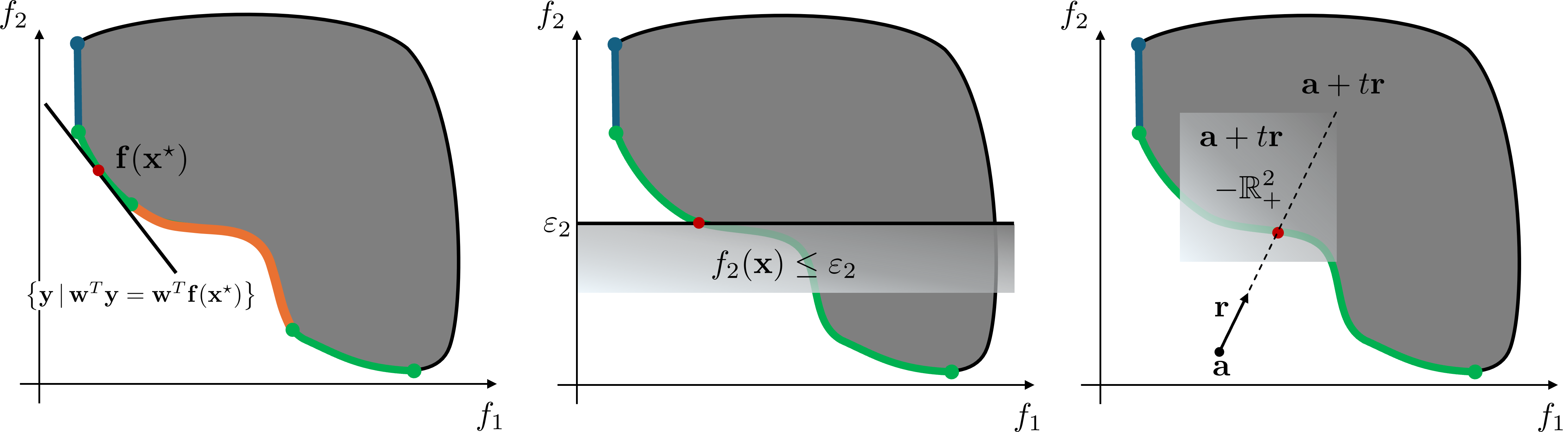
Scalarization methods transform MOP into a single-objective optimization problem that depends on one or more scalarization parameters. By varying these parameters, different efficient points are obtained. Scalarization thus replaces a multiobjective problem with a family of single-objective problems. A crucial property is if $\mathcal{E}$ can be completely recovered by varying the parameters. To this end, we introduce the recovery properties of the three scalarization methods studied in this work, namely weighted-sum scalarization [17], $\varepsilon$-constraint scalarization [18, 19] and the scalarization proposed by Pascoletti and Serafini [12]. The former two are selected due to their wide usage in topology optimization, as further discussed in Section 4. The latter is chosen because of its attractive theoretical properties. All three are illustrated in Figure 2.

Consider a rectangular domain $\Omega\subseteq\mathbb{R}^{2}$ of size $l_{x}$ by $l_{y}$, with $l_{x},l_{y}\in\mathbb{R}_{++}$, meshed with $n=n_{x}\times n_{y}$ square elements. The goal of topology optimization is to choose the physical design vector $\mathbf{x}_{P}\in\{0,1\}^{n}$, where an entry $x_{P,i}\in\{0,1\}$ corresponds to the density of element $i$. Elements with $x_{P,i}=1$ denote the presence of solid material and, conversely, elements with $x_{P,i}=0$ denote void, i.e., the absence of material.

To avoid solving an integer problem and allow the use of efficient gradient-based algorithms, the problem is relaxed to allow for continuous design variables: $\mathbf{x}_{P}\in[0,1]^{n}$. To prevent checkerboard patterns and enforce a length scale, we use the filtering scheme illustrated in Figure 3. The scheme employs the PDE filter from Lazarov and Sigmund [21] with the consistent boundary conditions from Wallin et al. [22] and the smoothed Heaviside projection [23], combined through the robust approach from Wang et al. [24]. Because of the robust approach, the Heaviside operator is performed at three different levels and hence produces three physical design vectors: the blueprint design $\mathbf{x}_{b}$, the eroded design $\mathbf{x}_{e}$ and the dilated design $\mathbf{x}_{d}$. The value of the objective and constraint functions are then defined by taking the maximum of the three designs. That is,

where the $\max$-operator is applied elementwise and $f$ and $\mathbf{g}$ are generic objective and constraint functions. A generic single-objective density-based topology optimization problem is thus formulated as

where $f:\mathbb{R}^{n}\rightarrow\mathbb{R}$ is the objective function and $\mathbf{g}:\mathbb{R}^{n}\rightarrow\mathbb{R}^{k}$ is a $k$-dimensional constraint. Both objective and constraint function values depend on $\mathbf{x}_{P}$, which is produced from $\mathbf{x}$ via the filter of Equation 3.

For the volume and compliance objectives, discussed below, the $\max$-operator reduces to the dilated volume and the eroded compliance. However, for the more challenging objectives studied in this work, namely dynamic compliance and maximum stress, the nondifferentiable $\max$ function is dealt with via a bound formulation and additional optimization variables. This is discussed in A. The compliance and volume objective functions are now briefly introduced.

The volume $V:\mathbb{R}^{n}\rightarrow\mathbb{R}$ is found by summing the density values,

The volume of the design domain, $V_{\max}\in\mathbb{R}$, is used to define the volume fraction $v:\mathbb{R}^{n}\rightarrow\mathbb{R}$

Thus, the constraint $v(\mathbf{x})\leq 0.5$ means that at most $50\%$ of the design domain can contain solid material. The robust filtering approach means the volume fraction is the maximum of the volume of the eroded, dilated and blueprint design. However, due to filter’s structure, the dilated design always has the largest volume [25]. Thus, $\max(v(\mathbf{x}_{b}(\mathbf{x})),v(\mathbf{x}_{e}(\mathbf{x})),v(\mathbf{x}_{d}(\mathbf{x})))=v(\mathbf{x}_{d}(\mathbf{x})):=v_{d}\in\mathbb{R}_{+}$.

Compliance is the oldest objective function in structural optimization, going back to the work of Michell [26]. It equals the work of the external forces and hence represents the inverse of the stiffness of the design. Compliance is here computed numerically via the finite element method. Consider again the rectangular finite element grid with $n=n_{x}\times n_{y}$ elements and thus $(n_{x}+1)\times(n_{y}+1)$ nodes. Each node $N_{i}$ has two associated degrees of freedom, its $x$ translation $u_{i,x}$ and $y$ translation $u_{i,y}$, for a total of $q=2(n_{x}+1)\times(n_{y}+1)$ degrees of freedom. These are collected in the displacement vector $\mathbf{u}\in\mathbb{R}^{q}$. We also introduce the external force vector $\mathbf{f}_{\mathrm{ext}}\in\mathbb{R}^{q}$. Finally, the stiffness matrix $\mathbf{K}(\mathbf{x})\in\mathbb{R}^{q\times q}$ is found by evaluating a map $\mathbb{R}^{n}\rightarrow\mathbb{R}^{q\times q}$ that sums the $n$ elemental stiffness matrices $\mathbf{K}_{i}\in\mathbb{R}^{q\times q}$:

Here, $p:\mathbb{R}\rightarrow\mathbb{R}$ is the Solid Isotropic Material with Penalization (SIMP) interpolation $p:=x\rightarrow\delta+(x-\delta)^{P}$ [27]. Here, $\delta$ is a small number to ensure $p(0)=\delta\neq 0$ and prevent ill-conditioning of $\mathbf{K}(\mathbf{x})$. The penalization $P\in\mathbb{R}_{+}$ is increased during optimization to drive the design towards black-white solutions. Numerical details are in B.

Using the above, we now write the state equation:

The state equation enforces linear elasticity and is enforced implicitly. That is, after the filtering operation provides a design vector $\mathbf{x}$, we construct $\mathbf{K}(\mathbf{x})$ and solve Equation 8. As a result, the state vector $\mathbf{u}$ depends implicitly on the design vector $\mathbf{x}$. To incorporate the Dirichlet boundary conditions, we select the nodes which lie on a fixed edge and set their corresponding degrees of freedom to zero. That is, for every fixed node $N_{i}$, we set $u_{i,x}=u_{i,y}=0$. Static condensation of $\mathbf{K}$ then yields a reduced system

where $\hat{\mathbf{u}},\hat{\mathbf{f}}_{\mathrm{ext}}\in\mathbb{R}^{q-\Delta q}$ and $\hat{\mathbf{K}}\in\mathbb{R}^{(q-\Delta q)\times(q-\Delta q)}$ with $\Delta q$ the number of fixed degrees of freedom. The compliance objective function is then defined as $c:=\mathbf{u}^{\top}\mathbf{f}_{\mathrm{ext}}\in\mathbb{R}_{+}$. Note that the compliance of the eroded design is always the largest [25] and therefore

This paper uses the shorthand notation $c(\mathbf{x}_{e}(\mathbf{x}))=c(\mathbf{x}_{e})=c_{e}\in\mathbb{R}$.

The compliance minimization problem is stated as follows.

Here, the state equation is satisfied implicitly and the filter produces $\mathbf{x}_{d}$ for the volume and $\mathbf{x}_{e}$ for the compliance. All topology optimization examples employ the Method of Moving Asymptotes (MMA) [28]. Interfacing between the employed scalarizations, as well as hyperparameters, are explained in A.

Because topology optimization is inherently nonconvex, it is difficult to draw strong conclusions in multiobjective contexts that rely on global optimality. To simplify the setting and illustrate the concept of local Pareto fronts, this section considers a truss optimization example.

Figure 5 shows three truss ground structures: a symmetric two- and eight-bar truss and an asymmetric four-bar truss. They represent three stable and non-crossing truss topologies for the considered boundary conditions. Note that although there exist other truss topologies, e.g. with five or six members, these were omitted for brevity.

Consider compliance and volume minimization of each of these truss layouts under a vertical load at the node on the far right (at $(x,y)=(2,0)$). The bar areas, collected in the bar area vector $\mathbf{a}_{\mathrm{bar}}$, must be optimized and a volume and length scale constraint is added. This leads to the following formulation.

For this section, $c$ and $v$ are redefined as the compliance and volume function dependent on the bar areas $\mathbf{a}_{\mathrm{bar}}$. The truss compliance is defined as $c(\mathbf{a}_{\mathrm{bar}})=\mathbf{u}^{\top}\mathbf{f}_{\mathrm{ext}}$ with $\mathbf{f}_{\mathrm{ext}}$ the external force vector and $\mathbf{u}$ the displacement vector. The latter is implicitly dependent on $\mathbf{a}_{\mathrm{bar}}$ via the state equation $\mathbf{K}(\mathbf{a}_{\mathrm{bar}})\mathbf{u}=\mathbf{f}$, where $\mathbf{K}=\sum_{i}a_{i}\mathbf{K}_{i}$ is a linearly weighted sum of elemental stiffness matrices.

The volume is $v(\mathbf{a}_{\mathrm{bar}})=\mathbf{a}_{\mathrm{bar}}^{\top}\mathbf{l}$, with $\mathbf{l}$ containing the bar lengths. The lower bound on the areas is uniform, i.e., $\mathbf{a}_{\min}=a_{\min}\mathbf{1}$ with $\mathbf{1}$ a vector of ones. It enforces a minimum length scale of $a_{\min}>0$.

The trusses are statically determinate and no member can vanish due to the length scale ($a_{\min}>0$), so $\mathbf{K}(\mathbf{a}_{\mathrm{bar}})$ is invertible and the compliance is convex in the bar areas. The volume constraint and compliance objective are linear in the bar areas and the length scale is a simple box constraint. Hence, the truss optimization problem of Equation 13 is convex [47]: local optima are also global optima.

Figure 6 shows the nondominated points when minimizing both volume and compliance, for each of the truss layouts. They are obtained by finding the individual minimum for the volume ($v_{\min}$ occurs at $\mathbf{a}_{\mathrm{bar}}=\mathbf{a}_{\min}$) and doing successive $\varepsilon$-constraint scalarizations between $v_{\min}$ and $v_{\max}$. For a fixed truss layout (two-bar, four-bar or eight-bar), the optimization problem of Equation 13 is from now on referred to as a truss subproblem. If the choice of the groundstructure is also considered, the problem is referred to as the truss superproblem. As stated, each subproblem is convex and hence the found solutions are globally optimal.

Figures 7(a) and 7(b) plot the nondominated points of each subproblem to illustrate the superproblem. Each truss layout thus represents a local optimum of the superproblem. In this multiobjective context, the Pareto frontier of each subproblem corresponds to a local Pareto frontier of the superproblem.

A crucial feature of the truss superproblem is that the globally optimal groundstructure depends on the volume. At high volumes (above $v(\mathbf{a})\approx 0.07$), the eight-bar symmetric truss is preferable. However, around $v(\mathbf{a}_{\mathrm{bar}})\approx 0.07$, this truss reaches $a_{\min}$ for all of its bars and hence no more feasible solutions exist with a lower volume. The optimal design switches from the symmetric eight-bar truss to the asymmetric four-bar truss, and then again to the symmetric 2-bar truss at $v(\mathbf{a}_{\mathrm{bar}})\approx 0.055$. The groundstructure switch also causes a discontinuity in the nondominated set: the compliance and stiffness jump when the ground structure changes. Finally, note that the volume-vs-stiffness frontiers are piecewise linear and that, in the pre-image space corresponding to each piece, the bars with an active minimum area constraint remain at $a_{\min}$ and the others scale linearly with $v(\mathbf{a}_{\mathrm{bar}})$.

When the node positions are also allowed to vary (see Figure 7), the nondominated set remains a collection of pieces stemming from each of the three truss layouts (two-bar at low $v(\mathbf{a}_{\mathrm{bar}})$, four-bar at medium $v(\mathbf{a}_{\mathrm{bar}})$ and eight-bar at high $v(\mathbf{a}_{\mathrm{bar}})$). However, the additional design freedom leads to (i) a more concave nondominated set $\mathcal{N}$, (ii) a nonlinear relation between volume and stiffness due to changing node positions and (iii) a continuous switch from one piece to another in the image space since the Pareto frontiers of each set now cross each other..

The remainder of the numerical examples consider topology optimization. This section considers the cantilever example of Figure 4, but only focuses on the volume $v(\mathbf{x}_{d})$ and the compliance $c_{1}(\mathbf{x}_{e})$ under the first load case, for the remainder of this section simply referred to as $c(\mathbf{x}_{e})$. Since compliance can become unbounded, it is bounded by $5c_{\mathrm{solid}}$, with $c_{\mathrm{solid}}=c(\mathbf{1})$ the compliance of the fully solid structure. The optimization problem is then written as

where $x_{i}=1$ for the elements in the $b$ by $b$ square (see Figure 4).

This section studies compliance minimization of the cantilever of Figure 4 under two load cases: a vertical and a compressive load. To limit compliance, an upper bound of $10$ times the solid compliance is added for both load cases. The volume is constrained to prevent convergence to the trivial solution of $v(\mathbf{x})=100\%$. This yields the following formulation.

The Pareto frontier is approximated with weighted-sum, $\varepsilon$-constraint and Pascoletti-Serafini scalarization, each with $30$ points, and the results are shown in Figure 13 for $v_{\max}=50\%$. Weighted-sum scalarization again shows a clustered Pareto frontier and the two $\varepsilon$-constraint variants each miss out on one “leg” of the frontier. In contrast, Pascoletti-Serafini scalarization leads to a much more uniform approximation.

Looking at the image space, it is notable that the approximated Pareto frontier is slightly nonconvex: point (c) lies above the line connecting point (b) and (e). Due to the many local optima in topology optimization, it is unclear if the actual Pareto frontier is also nonconvex.

Comparing the image and design space, it is clear that the obtained points belong to distinct local frontiers. Design (b) and (c) have the same topology (an internal cross) and hence belong to the same local frontier. However, going from design (c) to (e) leads to a change in topology and hence a change in local frontier: either the internal cross is replaced by a single diagonal bar (design $(\mathrm{d}_{1})$) or the cross moves to the right (design $(\mathrm{d}_{2})$). Moving from design $(\mathrm{d}_{1})$ or $(\mathrm{d}_{2})$ to (e) requires an additional topological change: the internal structure is removed, leaving only the two outer bars. Finally, going from design (e) to (f) and eventually (g) sees a slow merging of the two beams until only a single one remains. Note that at the top left side of the frontier, design (a) is a single dominated local optimum containing a double internal cross.

Figure 14 shows the same study carried out at $v_{\max}=30\%$. Three differences to the previous $v_{\max}=50\%$ case are noteworthy.

First, the compliance upper bound of $10c_{1}(\mathbf{1})$ is now reached, for example by design (h). This causes a single beam design, such as design (g) in Figure 13, to be no longer feasible. Instead, the transition from design (g) to (h) sees the transformation from a symmetric two-beam design to an asymmetric two-beam design. The asymmetry seems necessary for optimality: design (i) found by Pascoletti-Serafini scalarization retains symmetry and is strongly dominated.

Second, several topologies and local frontiers found at $v_{\max}=50\%$ reappear for $v_{\max}=30\%$, although they are now partly dominated. Consider for example the transition of point (a) to (b) and then ($\mathrm{c}_{1}$), which corresponds to a design with an internal cross whose outer bars become straight. This resembles the transition from design (b) to (c) in Figure 13, but in Figure 14 the corresponding points are now dominated by point (f). The transitions from ($\mathrm{c}_{1}$) to ($\mathrm{d}_{1}$) and ($\mathrm{c}_{2}$) to ($\mathrm{d}_{2}$), as well as the appearance of either asymmetry (design ($\mathrm{e}_{1}$)) or an internal cross that moves to the right (design ($\mathrm{e}_{2}$)) is similar to before but now dominated.

Third, as a result of the many dominated local optima, the approximation of the nondominated set ($\tilde{\mathcal{N}}$) contains a wide gap between point (f) and (g). It is unclear whether nondominated points exist in this region. This could be further investigated by solving Equation $\mathrm{PS}(\mathbf{a},\mathbf{r})$ for more values of $\mathbf{a}$, using a tracing method (Section 5.2.2) or starting from multiple initial guesses (Section 5.2.4).

To study the effect of more difficult objective functions, this section considers the trade-off between compliance and the maximum stress. Consider the L-shaped design domain of Figure 15, with $l_{x}=l_{y}=1$ and meshed with square elements of size $1/200$ by $1/200$ for a total of $n=\frac{3}{4}200^{2}=30000$. The $b$ by $b$ region consists of $10$ by $10$ solid elements on which a downward force of size $1$ is applied. The volume fraction is bounded from above by $v_{\max}=50\%$. The objectives are the compliance under the applied load and the maximum stress.

After application of the load, each element $k$ in the L-shaped design domain has an associated Von Mises stress $\sigma_{k,\mathrm{VM}}$, defined at the element center. The elemental stresses are aggregated into the aggregated stress function $s(\mathbf{x})\approx\max(\{\sigma_{1,\mathrm{VM}},\ldots,\sigma_{n,\mathrm{VM}}\})$. This work employs the function of Kreisselmeier and Steinhauser [55] to provide a differentiable approximation of the maximum stress among the elements. Due to the filtering approach, the maximum must also be taken over the eroded, dilated and blueprint design (see Equation 3). To circumvent the nondifferentiability of the $\max$ operator, additional optimization variables are used, with details in A.

The compliance and stress minimization problem is formulated as

where $\mathbf{x}$ is fixed at $1$ for those entries corresponding to the $100$ elements in the $b$ by $b$ solid region. Continuation and material parameters are in C.

Figure 16 shows the Pareto frontier approximation obtained with twenty points of the weighted-sum, $\varepsilon$-constraint and Pascoletti-Serafini scalarization. With the weighted-sum scalarization, the approximate nondominated set consists of two parts, with a large gap in between. The high-stress, low-compliance part corresponds to designs that stick to the sharp corner. The low-stress, high-compliance part consists of designs fully detached from this corner. Curiously, the three highest-compliance designs (with $c(\mathbf{x})>2.4c_{\mathrm{solid}}$) are dominated by some of the stiffer designs. This has knock-on effects for the other scalarizations since they consider these dominated designs to be the endpoints of the nondominated set. In particular, the “$\min c(\mathbf{x})$” variant of the $\varepsilon$-constraint scalarization yields an approximation of the nondominated set that does not cover the lowest-stress region. The “$\min s(\mathbf{x})$” variant has a cluster of points around $c(\mathbf{x})\approx 2.45c_{\mathrm{solid}}$, where the compliance constraint is inactive. The Pascoletti-Serafini also clusters in this region for the same reason.

Regarding overall approximation quality, the Pascoletti-Serafini scalarization is superior: it finds points uniformly along the complete nondominated set. However, three low-compliance points are slightly dominated, possibly due to the same convergence issues noted before (e.g., Section 5.2.3).

This section applies weighted-sum, $\varepsilon$-constraints and Pascoletti-Serafini scalarization to the minimization of compliance $c(\mathbf{x})$ and dynamic compliance $d(\mathbf{x})$ of a $2$-by-$1$ cantilever with volume fraction $v(\mathbf{x})\leq 0.5$. For brevity, most numerical details are moved to D. Figure 17 shows the obtained results.

The nondominated set has a long flat portion at low dynamic compliance, cut short due to the compliance constraint at $c(\mathbf{x}_{e})=10c_{\mathrm{solid}}$. This complicates its approximation, although in a different way depending on the scalarization technique. The weighted-sum scalarization produces a very clustered approximation of the nondominated set, leaving a large gap between $c(\mathbf{x}_{e})/c_{\mathrm{solid}}=4$ and $10$. The compliance minimization (“$\min c(\mathbf{x})$”) variant of the $\varepsilon$-constraint scalarization nicely approximates the low compliance portion of the nondominated set, but leaves larger holes at higher compliance due to the steepness of the nondominated set. The dynamic compliance minimization (“$\min d(\mathbf{x})$”) variant sees the opposite effect: good approximation of the low dynamic compliance portion but relatively few points in the high dynamic compliance region. The Pascoletti-Serafini scalarization provides a marginally better spacing in the low compliance region. The difference with respect to the “$\min d(\mathbf{x})$” is however limited due to the large difference between the two objective functions: lines $\mathbf{p}=\left\{\mathbf{a}+t\mathbf{r}\,|\,t\in\mathbb{R}\right\}$ are almost vertical. Additionally, it also produces several dominated points due to a slower convergence speed.

Resources and services were provided by the VSC (Flemish Supercomputer Center), funded by the Research Foundation - Flanders (FWO) and the Flemish Government. The research stay of T. De Weer was funded by FWO grant V456025N. Financial support from the Villum Foundation through the Villum Investigator Project AMSTRAD (VIL54487) is gratefully acknowledged.

On behalf of all authors, the corresponding author states that there is no conflict of interest.

All authors contributed to the study conceptualization and design, commented on previous versions and read and approved the final version. Data collection, analysis and writing was performed by the corresponding author.

Not applicable.

Methodological details are described to facilitate the replication of the results. Data will be made available on request.

References

- [1] M. P. Bendsøe, N. Kikuchi, Generating optimal topologies in structural design using a homogenization method, Computer Methods in Applied Mechanics and Engineering 71 (2) (1988) 197–224.
- [2] P. Duysinx, M. P. Bendsøe, Topology optimization of continuum structures with local stress constraints, International Journal for Numerical Methods in Engineering 43 (8) (1998) 1453–1478.
- [3] G. A. da Silva, A. T. Beck, O. Sigmund, Stress-constrained topology optimization considering uniform manufacturing uncertainties, Computer Methods in Applied Mechanics and Engineering 344 (2019) 512–537.
- [4] M. M. Neves, H. C. Rodrigues, J. M. Guedes, Generalized topology design of structures with a buckling load criterion, Structural optimization 10 (1995) 71–78.
- [5] F. Ferrari, O. Sigmund, Revisiting topology optimization with buckling constraints, Structural and Multidisciplinary Optimization 59 (2019) 1401–1415.
- [6] A. R. Díaaz, N. Kikuchi, Solutions to shape and topology eigenvalue optimization problems using a homogenization method, International Journal for Numerical Methods in Engineering 35 (7) (1992) 1487–1502.
- [7] T. Borrvall, J. Petersson, Topology optimization of fluids in stokes flow, International Journal for Numerical Methods in Fluids 41 (1) (2003) 77–107.
- [8] V. Cool, O. Sigmund, N. Aage, F. Naets, E. Deckers, Vibroacoustic topology optimization for sound transmission minimization through sandwich structures, Journal of Sound and Vibration 568 (2024) 117959.
- [9] J. Jensen, O. Sigmund, Topology optimization for nano-photonics, Laser & Photonics Reviews 5 (2) (2011) 308–321.
- [10] M. Ehrgott, Multicriteria Optimization, 2nd Edition, Springer, Berlin, Heidelberg, 2005.
- [11] G. Eichfelder, Twenty years of continuous multiobjective optimization in the twenty-first century, EURO Journal on Computational Optimization 9 (2021) 100014.
- [12] A. Pascoletti, P. Serafini, Scalarizing vector optimization problems, Journal of Optimization Theory and Applications 42 (1984) 499–524.
- [13] K. Miettinen, Nonlinear Multiobjective Optimization, 1st Edition, Springer, New York, 1998.
- [14] G. Eichfelder, Adaptive Scalarization Methods in Multiobjective Optimization, 1st Edition, Springer, Berlin, Heidelberg, 2008.
- [15] F. Y. Edgeworth, Mathematical Psychics, McMaster University Archive for the History of Economic Thought, 1881.
- [16] V. Pareto, Cours d’Economie Politique, 1898.
- [17] L. Zadeh, Optimality and non-scalar-valued performance criteria, IEEE Transactions on Automatic Control 8 (1) (1963) 59–60.
- [18] Y. Y. Haimes, L. S. Lasdon, D. A. Wismer, On a bicriterion formulation of the problems of integrated system identification and system optimization, IEEE Transactions on Systems, Man, and Cybernetics 1 (3) (1971) 296–297.
- [19] S. A. Marglin., Public Investment Criteria, MIT press, Cambridge, 1969.
- [20] G. Eichfelder, Scalarizations for adaptively solving multi-objective optimization problems, Computational Optimization and Applications 44 (2009) 249–273.
- [21] B. S. Lazarov, O. Sigmund, Filters in topology optimization based on helmholtz-type differential equations, International Journal for Numerical Methods in Engineering 86 (6) (2011) 765–781.
- [22] M. Wallin, N. Ivarsson, O. Amir, D. Tortorelli, Consistent boundary conditions for pde filter regularization in topology optimization, Structural and Multidisciplinary Optimization 62 (2020) 1299–1311.
- [23] J. K. Guest, J. H. Prévost, T. Belytschko, Achieving minimum length scale in topology optimization using nodal design variables and projection functions, International Journal for Numerical Methods in Engineering 61 (2) (2004) 238–254.
- [24] F. Wang, B. S. Lazarov, O. Sigmund, On projection methods, convergence and robust formulations in topology optimization, Structural and Multidisciplinary Optimization 43 (6) (2011) 767–784.
- [25] B. S. Lazarov, F. S. Wang, O. Sigmund, Length scale and manufacturability in density-based topology optimization, Archive of Applied Mechanics 86 (2016) 189–218.
- [26] A. Michell, The limits of economy of material in frame-structures, Philosophical Magazine 8 (47) (1904) 589–597.
- [27] M. Bendsøe, Optimal shape design as a material distribution problem, Structural Optimization 1 (1989) 193–202.
- [28] K. Svanberg, The method of moving asymptotes—a new method for structural optimization, International Journal for Numerical Methods in Engineering 24 (2) (1987) 359–373.
- [29] T. Cheng, X. Wu, Multiobjective optimal topology design of structures, Computational Mechanics 21 (6) (1998) 483–492.
- [30] D. M. De Lean, J. Alexandersen, J. S. O. Fonseca, O. Sigmund, Stress-constrained topology optimization for compliant mechanism design, Structural and Multidisciplinary Optimization 52 (2015) 929–943.
- [31] Y. Sato, K. Izui, T. Yamada, S. Nishiwaki, Pareto frontier exploration in multiobjective topology optimization using adaptive weighting and point selection schemes, Structural and Multidisciplinary Optimization 55 (3) (2017) 409–422.
- [32] J. Wang, Y. Wang, L. Ma, X. Liu, Multi-objective topology optimization and flow characteristics study of the microfluidic reactor, Reaction Kinetics, Mechanisms and Catalysis 135 (5) (2022) 2475–2501.
- [33] C. F. Christensen, F. Wang, O. Sigmund, Topology optimization of multiscale structures considering local and global buckling response, Computer Methods in Applied Mechanics and Engineering 408 (2023) 115969.
- [34] D. Chen, P. Kumar, Y. Kametani, Y. Hasegawa, Multi-objective topology optimization of heat transfer surface using level-set method and adaptive mesh refinement in openfoam, International Journal of Heat and Mass Transfer 221 (2024) 125099.
- [35] C. Almeida, P. Coelho, J. Guedes, A. Custódio, F. Conde, A. Velhinho, Multiobjective topology optimization of metamaterials to analyse the conflicting nature of negative poisson’s ratio and negative thermal expansion, Structural and Multidisciplinary Optimization 68 (2025) 202.
- [36] E. Wotten, K. I. Yong, Multi-objective build orientation and topology optimization for cost and time minimization in fiber-reinforced additive manufacturing, Structural and Multidisciplinary Optimization 69 (2026) 73.
- [37] K. Suresh, A 199-line matlab code for pareto-optimal tracing in topology optimization, Structural and Multidisciplinary Optimization 42 (2010) 665–679.
- [38] F. Zhao, A meshless pareto-optimal method for topology optimization, Engineering Analysis with Boundary Elements 37 (12) (2013) 1625–1631.
- [39] M. Takalloozadeh, G. H. Yoon, Development of pareto topology optimization considering thermal loads, Computer Methods in Applied Mechanics and Engineering 317 (2017) 554–579.
- [40] M. Arifin, Nathan, L. Zuhal, A. Sumboya, P. Palar, Multi-objective robust topology optimization of metalenses via pareto optimal tracing and polynomial chaos, Structural and Multidisciplinary Optimization 68 (2025) 157.
- [41] F. Lucchini, R. Torchio, P. Alotto, Gradient-informed pareto-based multi-objective binary topology optimization, IEEE Access 13 (2025) 86576–86587.
- [42] T. Kunakote, S. Bureerat, Multi-objective topology optimization using evolutionary algorithms, Engineering Optimization 43 (5) (2011) 541–557.
- [43] H. L. Simonetti, V. S. Almeida, F. de Assis das Neves, M. Greco, Multi-objective topology optimization using the boundary element method, Structures 19 (2019) 84–95.
- [44] J. Lim, C. You, I. Dayyani, Multi-objective topology optimization and structural analysis of periodic spaceframe structures, Materials & Design 190 (2020) 108552.
- [45] N. Ryu, M. Seo, S. Min, Multi-objective topology optimization incorporating an adaptive weighed-sum method and a configuration-based clustering scheme, Computer Methods in Applied Mechanics and Engineering 385 (2021) 114015.
- [46] F. Crescenti, T. Kipouros, D. J. Munk, M. A. Savill, Generating minimal pareto sets in multi-objective topology optimisation: an application to the wing box structural layout, Structural and Multidisciplinary Optimization 63 (2021) 1119–1134.
- [47] K. Svanberg, On local and global minima in structural optimization, in: E. Atrek, R. Gallagher (Eds.), Proceedings of the International Symposium on Optimum Structural Design, Vol. 1, University of Arizona, 1981, pp. 6–3 to 6–10.
- [48] T. D. Weer, V. Cool, E. Deckers, Continuation strategies to mitigate convergence to low-performing local optima in dynamic topology optimization, Structural and Multidisciplinary Optimization 69 (2026) 148.
- [49] M. Stolpe, On some fundamental properties of structural topology optimization problems, Structural and Multidisciplinary Optimization 41 (5) (2010) 661–670.
- [50] G. Rozvany, On symmetry and non-uniqueness in exact topology optimization, Structural and Multidisciplinary Optimization 43 (2011) 297–317.
- [51] G. Cheng, X. Liu, Discussion on symmetry of optimum topology design, Structural and Multidisciplinary Optimization 44 (5) (2011) 713–717.
- [52] X. Guo, C. Ni, G. Cheng, Z. Du, Some symmetry results for optimal solutions in structural optimization, Structural and Multidisciplinary Optimization 46 (5) (2012) 631–645.
- [53] J. N. Richardson, S. Adriaenssens, P. Bouillard, R. Filomeno Coelho, Symmetry and asymmetry of solutions in discrete variable structural optimization, Structural and multidisciplinary optimization 47 (5) (2013) 631–643.
- [54] D. A. White, A. Voronin, A computational study of symmetry and well-posedness of structural topology optimization, Structural and Multidisciplinary Optimization 59 (2019) 759–766.
- [55] G. Kreisselmeier, R. Steinhauser, Systematic control design by optimizing a vector performance index, IFAC Proceedings Volumes 12 (7) (1979) 113–117.
- [56] X. Qian, O. Sigmund, Topological design of electromechanical actuators with robustness toward over-and under-etching, Computer Methods in Applied Mechanics and Engineering 253 (2013) 237–251.
- [57] G. D. Cheng, X. Guo, -relaxed approach in structural topology optimization, Structural Optimization 13 (4) (1997) 258–266.
- [58] N. L. Pedersen, Maximization of eigenvalues using topology optimization, Structural and Multidisciplinary Optimization 20 (1) (2000) 2–11.
- [59] R. E. Christiansen, B. S. Lazarov, J. S. Jensen, O. Sigmund, Creating geometrically robust designs for highly sensitive problems using topology optimization, Structural and Multidisciplinary Optimization 52 (4) (2015) 737–754.