Deep Projections and the Local Nature of the Cass Criterion

Leandro Lyra Braga Dognini Department of Economics, Rio de Janeiro State University Legislative Advisory, Federal Senate of Brazil

(June 14, 2026)

Abstract

This paper defines the deep projections of the indifference and the offer hypersurfaces. These projections are used to measure how much the trade hyperplane must be curved to reach these other two canonical manifolds. In particular, it is shown that the factor $\lambda_{n}(p)\partial e(p,v_{n}(p))/\partial u>0$ measures how much more bent the offer hypersurface is relative to the indifference hypersurface, where $\lambda_{n}(\cdot)$ is the Lagrange multiplier and $v_{n}(\cdot)$ is the indirect utility associated with the normalized Walrasian demand $x_{n}(\cdot)$ . These definitions and results are then applied to a consumption-loan overlapping generations economy to provide general statements for the sufficiency and necessity of the Cass criterion based on $\sum^{\infty}_{t=1}1/(\|p_{t}\|\sum_{h\in G_{t}}\|c^{h}_{t}\|)=\infty$ (thus allowing unbounded dynamics for both the demography and per capita endowments) under assumptions that reveal its local nature.

Keywords: Consumer Theory, General Equilibrium Theory, Overlapping Generations Economies, Differential Topology.

JEL: D11, D50.

1. Introduction

The canonical manifolds of consumer theory are the trade hyperplane, the indifference hypersurface, and the offer hypersurface. A natural and intuitive graphical description of the local behavior of these manifolds is the following: the trade hyperplane is the supporting hyperplane of both the indifference and the offer hypersurfaces, which are the boundaries of strictly convex sets that are strictly included one within the other.

With this depiction in mind, this paper shows that the indifference and offer hypersurfaces can be seen as curved versions of the trade hyperplane and defines the deep projections in order to quantify how bent the trade hyperplane must be to reach these other two manifolds. In particular, it is shown that the factor $\lambda_{n}(p)\partial e(p,v_{n}(p))/\partial u>0$ measures how much more bent the offer hypersurface is relative to the indifference hypersurface, where $\lambda_{n}(\cdot)$ is the Lagrange multiplier and $v_{n}(\cdot)$ is the indirect utility associated with the normalized Walrasian demand $x_{n}(\cdot)$ [8].

These projections serve as a complementary analytical tool for other well-known measures of curvature, as the Gaussian one (e.g., [7, pp. 612–613] and [15, pp. 39-40]), and an immediate application of them provides general statements for the necessity and sufficiency of the Cass criterion in consumption-loan overlapping generations economies [17].

It is well-known that in these overlapping generations economies all equilibria are weakly Pareto optimal [2, p. 286]. However, the First Welfare Theorem fails and they may be inefficient (e.g., [17, 5, 21]). Therefore, following [6], the literature has derived necessary and sufficient conditions to characterize efficient allocations (e.g., [3, 4, 2, 16, 11]) that are based on the asymptotic behavior of the supporting price sequence, in the form of

\displaystyle\sum^{\infty}_{t=1}\frac{1}{\|p_{t}\|}=\infty.

This statement of the Cass criterion assumes bounded dynamics for both the demography and per capita endowments. [11, pp. 1932–1936, Theorems 5a and 5b] derive a more general version that allows for unbounded demographic dynamics, which is given by

\displaystyle\sum^{\infty}_{t=1}\frac{1}{H_{t}\|p_{t}\|}=\infty,

with $H_{t}\in\mathbb{N}$ the number of households born at period $t\geq 1$ . This paper further generalizes the statement of the Cass criterion as

\displaystyle\sum^{\infty}_{t=1}\frac{1}{\|p_{t}\|\sum_{h\in G_{t}}\|c^{h}_{t}\|}=\infty,

(1)

thus allowing for unbounded dynamics for both the demography and per capita endowments. Reaching a more general statement for the Cass criterion is a relevant milestone for properly deploying overlapping generations models, which are used for a wide range of economic applications stemming from monetary theory (e.g., [13, 20, 9]) to the literature on bubbles (e.g., [22, 19, 12]) and social security design (e.g., [18, 10]).

Furthermore, the assumptions that support the general statement (1) are presented “on demand” in a step-by-step proof that highlights either their pointwise or local nature. Pointwise assumptions are those that depend only on the allocation and the supporting price sequence, whereas local assumptions depend on the behavior of the indifference hypersurfaces in a neighborhood of each household allocation. These local assumptions thus reveal the local nature of the Cass criterion and are all backed by results derived from the deep projections (see Theorems 6 and 7).

After this Introduction, the outline of the paper is as follows. Section 2 defines and characterizes the local behavior of the deep projections. Section 3 derives the general statements for the sufficiency and necessity of the Cass criterion. Finally, a brief discussion of the results is presented in the Conclusion and all omitted proofs are stated in the Appendix.

2. The deep projections of the canonical manifolds

The consumption set¹¹1I follow [14] for classical demand theory definitions and results. is $X=\mathbb{R}^{L}_{+}$ , $L\geq 2$ , and preferences are defined through a smooth, strictly increasing, and strictly quasi-concave utility function $u:\mathbb{R}^{L}_{+}\rightarrow\mathbb{R}$ . The Walrasian demand function $x:\mathbb{R}^{L+1}_{++}\rightarrow\mathbb{R}^{L}_{+}$ is defined as

\displaystyle x(p,w)=\arg\max_{c\in\mathbb{R}^{L}_{+}}u(c)\textrm{ s.t. }p\cdot c\leq w,

(2)

and I assume $x(p,w)\in\mathbb{R}^{L}_{++}$ , $(p,w)\in\mathbb{R}^{L+1}_{++}$ (i.e., (2) has no corner solutions²²2I preferred to state this assumption rather than impose conditions that ensure it. For instance, if the utility functions are strongly monotonic, satisfy a strong bordered Hessian condition, and the indifference curves are closed in $\mathbb{R}^{L}$ , then this assumption is satisfied (e.g., [23, p. 2]).). I proceed with the following definition from [8].

Definition 1.

The normalized Walrasian demand $x_{n}:\mathbb{R}^{L}_{++}\rightarrow\mathbb{R}^{L}_{++}$ is given by $x_{n}(p)=x(p,1)$ .

The normalized Walrasian demand is a diffeomorphism that represents the consumer demand when prices are stated as percentages of his wealth. Let $\lambda(p,w)>0$ be the Lagrange multiplier of (2) and the indirect utility function $v:\mathbb{R}^{L+1}_{++}\rightarrow\mathbb{R}$ be given by $v(p,w)=u(x(p,w))$ . Following Definition 1, let $\lambda_{n}(p)=\lambda(p,1)$ and $v_{n}(p)=u(x_{n}(p))$ , $p\in\mathbb{R}^{L}_{++}$ .

The Hicksian demand function $h:\mathbb{R}^{L}_{++}\times\mathbb{R}\rightarrow\mathbb{R}^{L}_{+}$ is defined as

\displaystyle h(p,u)=\arg\min_{c\in\mathbb{R}^{L}_{+}}p\cdot c\textrm{\ s.t.\ }u(c)\geq u,

and I assume $h(p,u)\in\mathbb{R}^{L}_{++}$ , $(p,u)\in\mathbb{R}^{L}_{++}\times\mathbb{R}$ . The expenditure function $e:\mathbb{R}^{L}_{++}\times\mathbb{R}\rightarrow\mathbb{R}_{++}$ is $e(p,u)=ph(p,u)^{T}$ . To ease notation, I write $\nabla e(p,u)=(\nabla_{1}e(p,u),\nabla_{2}e(p,u))\in\mathbb{R}^{L}_{++}\times\mathbb{R}_{++}$ , $\mathbf{H}_{11}e(p,u)=\mathbf{J}_{1}\nabla_{1}e(p,u)\in\mathbb{R}^{L\times L}$ and $\mathbf{H}_{21}e(p,u)=\partial\nabla_{1}e(p,u)/\partial u\in\mathbb{R}^{L}$ . The following result is taken from [8] (see it for a detailed proof and discussion of these definitions and their relations to the consumption, normalized and flat domains).

Proposition 1.

Let $x_{n}(\cdot)$ , $v_{n}(\cdot)$ , $\lambda_{n}(\cdot)$ , $h(\cdot)$ and $e(\cdot)$ be as defined above. Then, for $p,c\in\mathbb{R}^{L}_{++}$ , $u\in\mathbb{R}$ : (i) $\nabla_{1}e(p,u)=h(p,u)$ and $p\mathbf{H}_{11}e(p,u)=0$ ; (ii) $p\cdot x_{n}(p)=1$ , $p\mathbf{J}x_{n}(p)=-x_{n}(p)$ and $\lambda_{n}(p)=\nabla u(x_{n}(p))\cdot x_{n}(p)$ ; (iii) $x_{n}(p)=\nabla v_{n}(p)/p\cdot\nabla v_{n}(p)$ , $p\cdot\nabla v_{n}(p)=-\lambda_{n}(p)$ , and $x_{n}^{-1}(c)=\nabla u(c)/c\cdot\nabla u(c)$ ; and, (iv) $x_{n}(p)=h(p,v_{n}(p))$ , $h(p,u)=x_{n}(p/e(p,u))$ and $e(p,v_{n}(p))=1$ .

I proceed with the following definition.

Definition 2.

The canonical manifolds through $c\in\mathbb{R}^{L}_{++}$ are:

(i)

The indifference hypersurface, given by $\mathcal{I}(c)=\{y\in\mathbb{R}^{L}_{++}\mid u(y)=u(c)\}$ ;
(ii)

The offer hypersurface, given by $\mathcal{O}(c)=\{y\in\mathbb{R}^{L}_{++}\mid\nabla u(y)(y-c)^{T}=0\}$ ;
(iii)

The trade hyperplane, given by $\mathcal{H}(c)=\{y\in\mathbb{R}^{L}_{++}\mid\nabla u(c)(y-c)^{T}=0\}$ .

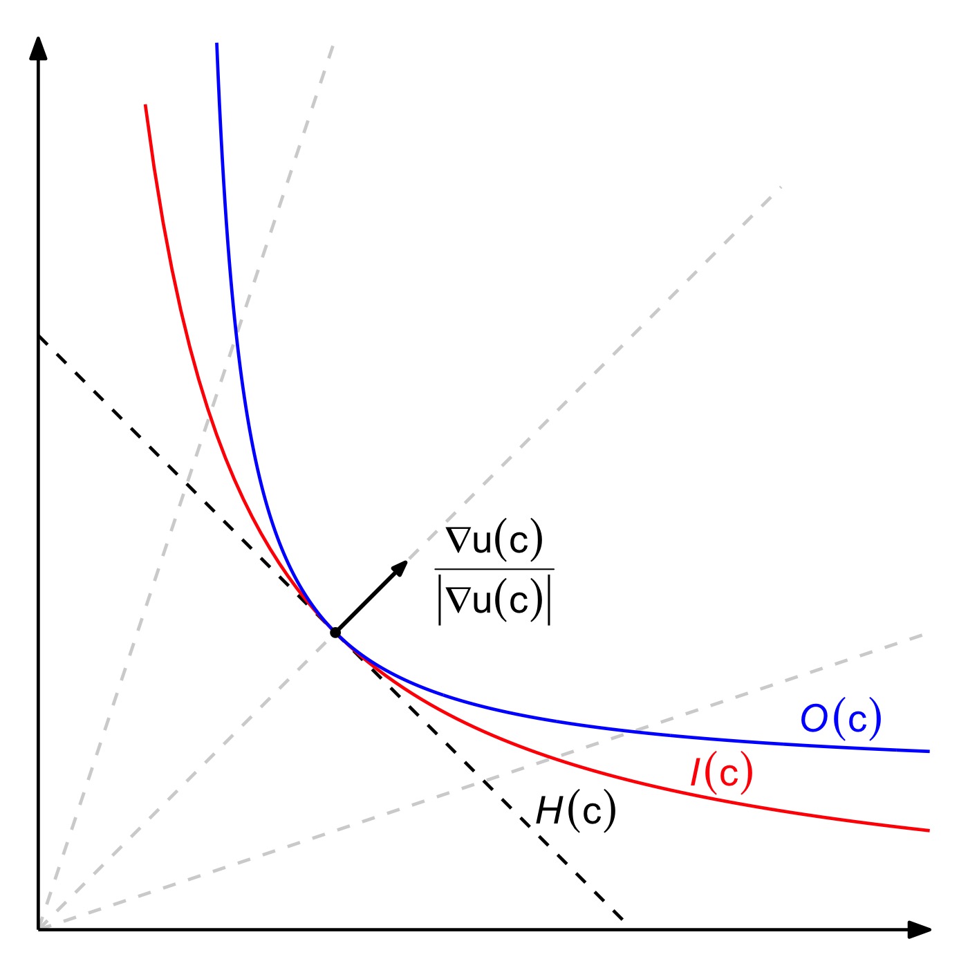
The three canonical manifolds are connected $L-1$ -dimensional manifolds with a single intersection at $c\in\mathbb{R}^{L}_{++}$ . Furthermore, the indifference and the offer hypersurfaces can be written as $\mathcal{I}(c)=\{h((q,1),u(c))\mid q\in\mathbb{R}^{L-1}_{++}\}$ and $\mathcal{O}(c)=\{x_{n}((q,1)/(q,1)\cdot c)\mid q\in\mathbb{R}^{L-1}_{++}\}$ [8, Proposition 5]. Figure 1 depicts the canonical manifolds through $c=(1,1)$ for $u(c)=c_{1}c_{2}$ .

Refer to caption — Figure 1: Graphical depiction of the canonical manifolds through $c=(1,1)$ for $u(c)=c_{1}c_{2}$ .

The gray dotted rays in Figure 1 are wealth expansion paths ([14, p. 25]) and lead us to note that these paths, for any given relative prices, intersect each of the three canonical manifolds at a unique point. By associating these points, one can see the indifference hypersurface as a bent version of the trade hyperplane around the point $c=(1,1)$ .

Further bending the indifference hypersurface thus leads us to the offer hypersurface, and the degree to which the trade hyperplane is curved can be measured by how far the projection along $\nabla u(c)/\|\nabla u(c)\|$ “runs deep” into the interior of the convex sets. This motivates the following definition.

Definition 3.

For $c\in\mathbb{R}^{L}_{++}$ , the deep projections of the indifference hypersurface $\mathcal{I}(c)$ , $\pi_{i}:\mathbb{R}^{L-1}_{++}\rightarrow\mathbb{R}_{+}$ , and of the offer hypersurface $\mathcal{O}(c)$ , $\pi_{o}:\mathbb{R}^{L-1}_{++}\rightarrow\mathbb{R}_{+}$ , are given by

	$\displaystyle\pi_{i}(q)$	$\displaystyle=$	$\displaystyle\frac{\nabla u(c)}{\\|\nabla u(c)\\|}\cdot(h((q,1),u(c))-c)$
	$\displaystyle\pi_{o}(q)$	$\displaystyle=$	$\displaystyle\frac{\nabla u(c)}{\\|\nabla u(c)\\|}\cdot\biggr(x_{n}\biggr(\frac{(q,1)}{(q,1)\cdot c}\biggr)-c\biggr),$

for $q\in\mathbb{R}^{L-1}_{++}$ .

For $p\in\mathbb{R}^{L}_{++}$ , it is convenient to define the auxiliary functions $\eta:\mathbb{R}^{L}_{++}\rightarrow\mathbb{R}_{+}$ and $\omega:\mathbb{R}^{L}_{++}\rightarrow\mathbb{R}_{+}$ as

	$\displaystyle\eta(q)$	$\displaystyle=$	$\displaystyle p\cdot(h(q,v_{n}(p))-x_{n}(p))$
	$\displaystyle\omega(q)$	$\displaystyle=$	$\displaystyle p\cdot\biggr(x_{n}\biggr(\frac{q}{q\cdot x_{n}(p)}\biggr)-x_{n}(p)\biggr).$

Notice that, for $c=x_{n}(p)\in\mathbb{R}^{L}_{++}$ , we have $\pi_{i}(q)=\|p\|\eta(q,1)$ and $\pi_{o}(q)=\|p\|\omega(q,1)$ . The next theorem characterizes the local behavior of these auxiliary functions.

Theorem 2.

Let $p\in\mathbb{R}^{L}_{++}$ , $\eta(\cdot)$ and $\omega(\cdot)$ be as defined above. Then, $\eta(p)=\omega(p)=0$ , $\nabla\eta(p)=\nabla\omega(p)=0$ , $\mathbf{H}\eta(p)=-\mathbf{H}_{11}e(p,v_{n}(p))$ , and

\displaystyle\mathbf{H}\omega(p)=-\biggr(1+\lambda_{n}(p)\frac{\partial e(p,v_{n}(p))}{\partial u}\biggr)\mathbf{H}_{11}e(p,v_{n}(p)).

The following example illustrates Theorem 2.

Example 1.

Let $u:\mathbb{R}^{2}_{++}\rightarrow\mathbb{R}$ be given by $u(c)=c_{1}c_{2}$ . The normalized Walrasian demand is $x_{n}(p)=(1/2p_{1},1/2p_{2})$ , $\lambda_{n}(p)=1/2p_{1}p_{2}$ , and the normalized indirect utility function is $v_{n}(p)=1/4p_{1}p_{2}$ , $p\in\mathbb{R}^{2}_{++}$ . The Hicksian demand function is $h(p,u)=(\sqrt{up_{2}/p_{1}},\sqrt{up_{1}/p_{2}})$ and the expenditure function is $e(p,u)=2\sqrt{p_{1}p_{2}u}$ , $(p,u)\in\mathbb{R}^{3}_{++}$ . Notice that

\displaystyle\mathbf{H}_{11}e(p,v_{n}(p))=\frac{1}{4p_{1}p_{2}}\begin{bmatrix}-\dfrac{p_{2}}{p_{1}}&1\\ 1&-\dfrac{p_{1}}{p_{2}}\end{bmatrix},

which is negative semi-definite and has eigenvalues $\mu_{1}=0$ and $\mu_{2}=-\|p\|^{2}/4p_{1}^{2}p_{2}^{2}$ , $p\in\mathbb{R}^{2}_{++}$ . Next, we have

\displaystyle\eta(q)=\frac{1}{2}\sqrt{\frac{p_{1}q_{2}}{p_{2}q_{1}}}+\frac{1}{2}\sqrt{\frac{p_{2}q_{1}}{p_{1}q_{2}}}-1,

so that

\displaystyle\nabla\eta(q)=\biggr(-\frac{1}{4}\sqrt{\frac{p_{1}q_{2}}{p_{2}q_{1}^{3}}}+\frac{1}{4}\sqrt{\frac{p_{2}}{p_{1}q_{1}q_{2}}},\frac{1}{4}\sqrt{\frac{p_{1}}{p_{2}q_{1}q_{2}}}-\frac{1}{4}\sqrt{\frac{p_{2}q_{1}}{p_{1}q_{2}^{3}}}\biggr)

and

\displaystyle\mathbf{H}\eta(q)=\begin{bmatrix}\dfrac{3}{8}\sqrt{\dfrac{p_{1}q_{2}}{p_{2}q_{1}^{5}}}-\dfrac{1}{8}\sqrt{\dfrac{p_{2}}{p_{1}q_{1}^{3}q_{2}}}&-\dfrac{1}{8}\sqrt{\dfrac{p_{1}}{p_{2}q_{1}^{3}q_{2}}}-\dfrac{1}{8}\sqrt{\dfrac{p_{2}}{p_{1}q_{1}q_{2}^{3}}}\\ -\dfrac{1}{8}\sqrt{\dfrac{p_{1}}{p_{2}q_{1}^{3}q_{2}}}-\dfrac{1}{8}\sqrt{\dfrac{p_{2}}{p_{1}q_{1}q_{2}^{3}}}&-\dfrac{1}{8}\sqrt{\dfrac{p_{1}}{p_{2}q_{1}q_{2}^{3}}}+\dfrac{3}{8}\sqrt{\dfrac{p_{2}q_{1}}{p_{1}q_{2}^{5}}}\end{bmatrix},

for $q\in\mathbb{R}^{2}_{++}$ . Therefore, $\eta(p)=0$ , $\nabla\eta(p)=0$ and

\displaystyle\mathbf{H}\eta(p)=\begin{bmatrix}\dfrac{1}{4p_{1}^{2}}&-\dfrac{1}{4p_{1}p_{2}}\\ -\dfrac{1}{4p_{1}p_{2}}&\dfrac{1}{4p_{2}^{2}}\end{bmatrix}=-\frac{1}{4p_{1}p_{2}}\begin{bmatrix}-\dfrac{p_{2}}{p_{1}}&1\\ 1&-\dfrac{p_{1}}{p_{2}}\end{bmatrix}=-\mathbf{H}_{11}e(p,v_{n}(p)).

Next, we have

\displaystyle\omega(q)=\frac{p_{1}q_{2}}{4p_{2}q_{1}}+\frac{p_{2}q_{1}}{4p_{1}q_{2}}-\frac{1}{2},

so that

\displaystyle\nabla\omega(q)=\biggr(-\frac{p_{1}q_{2}}{4p_{2}q_{1}^{2}}+\frac{p_{2}}{4p_{1}q_{2}},\frac{p_{1}}{4p_{2}q_{1}}-\frac{p_{2}q_{1}}{4p_{1}q_{2}^{2}}\biggr),

and

\displaystyle\mathbf{H}\omega(q)=\begin{bmatrix}\dfrac{p_{1}q_{2}}{2p_{2}q_{1}^{3}}&-\dfrac{p_{1}}{4p_{2}q_{1}^{2}}-\dfrac{p_{2}}{4p_{1}q_{2}^{2}}\\ -\dfrac{p_{1}}{4p_{2}q_{1}^{2}}-\dfrac{p_{2}}{4p_{1}q_{2}^{2}}&\dfrac{p_{2}q_{1}}{2p_{1}q_{2}^{3}}\end{bmatrix},

for $q\in\mathbb{R}^{2}_{++}$ . Notice that $\partial e(p,v_{n}(p))/\partial u=p_{1}p_{2}/2$ , so that $\lambda_{n}(p)\partial e(p,v_{n}(p))/\partial u=1$ . Therefore, $\omega(p)=0$ , $\nabla\omega(p)=0$ and

\displaystyle\mathbf{H}\omega(p)=\begin{bmatrix}\dfrac{1}{2p_{1}^{2}}&-\dfrac{1}{2p_{1}p_{2}}\\ -\dfrac{1}{2p_{1}p_{2}}&\dfrac{1}{2p_{2}^{2}}\end{bmatrix}=-2\mathbf{H}_{11}e(p,v_{n}(p))=-\biggr(1+\lambda_{n}(p)\frac{\partial e(p,v_{n}(p))}{\partial u}\biggr)\mathbf{H}_{11}e(p,v_{n}(p)).

Before stating the next result, it is convenient to define $f:\mathbb{R}^{L}_{++}\rightarrow\mathbb{R}^{L-1}_{++}$ as³³3It is important to notice that this auxiliary function is not the flattening diffeomorphism from [8] (although it coincides with the first $L-1$ coordinates of it).

\displaystyle f(x)=\frac{\nabla_{L-1}u(x)}{\partial_{L}u(x)}

for $x\in\mathbb{R}^{L}_{++}$ , and $M=\begin{bmatrix}I&0\end{bmatrix}\in\mathbb{R}^{(L-1)\times L}$ , with $I\in\mathbb{R}^{(L-1)\times(L-1)}$ the identity matrix. An immediate corollary of Theorem 2 is the following.

Corollary 3.

Let $c\in\mathbb{R}^{L}_{++}$ , $p=x_{n}^{-1}(c)$ , $\pi_{i}(\cdot)$ , $\pi_{o}(\cdot)$ and $f(\cdot)$ be as defined above. Then, $\pi_{i}(f(c))=0$ , $\pi_{o}(f(c))=0$ , $\nabla\pi_{i}(f(c))=0$ , $\nabla\pi_{o}(f(c))=0$ , and

	$\displaystyle\mathbf{H}\pi_{o}(f(c))$	$\displaystyle=$	$\displaystyle-\biggr(1+\lambda_{n}(p)\frac{\partial e(p,v_{n}(p))}{\partial u}\biggr)\frac{p_{L}^{2}}{\\|p\\|}M\mathbf{H}_{11}e(p,v_{n}(p))M^{T}$
		$\displaystyle=$	$\displaystyle\biggr(1+\lambda_{n}(p)\frac{\partial e(p,v_{n}(p))}{\partial u}\biggr)\mathbf{H}\pi_{i}(f(c)),$

for $p=x_{n}^{-1}(c)$ .

Corollary 3 reveals that the factor $\lambda_{n}(p)\partial e(p,v_{n}(p))/\partial u>0$ measures how much more bent around $c\in\mathbb{R}^{L}_{++}$ the offer hypersurface is relative to the indifference hypersurface. The following example illustrates Corollary 3.

Example 2.

I build on Example 1. For $c\in\mathbb{R}^{2}_{++}$ , Definition 3 implies

	$\displaystyle\pi_{i}(q)$	$\displaystyle=$	$\displaystyle\sqrt{\frac{c_{1}c_{2}}{q(c_{1}^{2}+c_{2}^{2})}}(\sqrt{c_{2}}-\sqrt{qc_{1}})^{2}$
	$\displaystyle\pi_{o}(q)$	$\displaystyle=$	$\displaystyle\frac{(c_{2}-qc_{1})^{2}}{2q\sqrt{c_{1}^{2}+c_{2}^{2}}}$

for $q>0$ . Also, $f(c)=\partial_{1}u(c)/\partial_{2}u(c)=c_{2}/c_{1}$ and, therefore, $\pi_{i}(f(c))=\pi_{o}(f(c))=0$ . Next,

	$\displaystyle\pi_{i}^{\prime}(q)$	$\displaystyle=$	$\displaystyle-\frac{1}{2}\sqrt{\frac{c_{1}c_{2}}{q^{3}(c_{1}^{2}+c_{2}^{2})}}(\sqrt{c_{2}}-\sqrt{qc_{1}})^{2}-\sqrt{\frac{c_{1}c_{2}}{q(c_{1}^{2}+c_{2}^{2})}}(\sqrt{c_{2}}-\sqrt{qc_{1}})\sqrt{\frac{c_{1}}{q}}$
	$\displaystyle\pi_{o}^{\prime}(q)$	$\displaystyle=$	$\displaystyle-\frac{(c_{2}-qc_{1})^{2}}{2q^{2}\sqrt{c_{1}^{2}+c_{2}^{2}}}-\frac{(c_{2}-qc_{1})}{q\sqrt{c_{1}^{2}+c_{2}^{2}}}c_{1}$

for $q>0$ . Therefore, $\pi_{i}^{\prime}(f(c))=\pi_{o}^{\prime}(f(c))=0$ . Finally, notice that

	$\displaystyle\pi^{\prime\prime}_{i}(f(c))$	$\displaystyle=$	$\displaystyle\frac{c_{1}^{3}}{2c_{2}\sqrt{c_{1}^{2}+c_{2}^{2}}}$
	$\displaystyle\pi^{\prime\prime}_{o}(f(c))$	$\displaystyle=$	$\displaystyle\frac{c_{1}^{3}}{c_{2}\sqrt{c_{1}^{2}+c_{2}^{2}}}.$

Since $p=x_{n}^{-1}(c)=(1/2c_{1},1/2c_{2})$ and $\lambda_{n}(p)\partial e(p,v_{n}(p))/\partial u=1$ , we have

\displaystyle-\frac{p_{2}^{2}}{\|p\|}M\mathbf{H}_{11}e(p,v_{n}(p))M^{T}=\frac{p_{2}^{2}}{\|p\|}\frac{1}{4p_{1}^{2}}=\frac{c_{1}^{3}}{2c_{2}\sqrt{c_{1}^{2}+c_{2}^{2}}}=\pi^{\prime\prime}_{i}(f(c))=\frac{\pi^{\prime\prime}_{o}(f(c))}{2}.

The next result uses the Taylor expansion to provide upper and lower bounds for the deep projections in a neighborhood of $c\in\mathbb{R}^{L}_{++}$ .

Proposition 4.

Let $c\in\mathbb{R}^{L}_{++}$ , $p=x^{-1}_{n}(c)$ , $\pi_{i}(\cdot)$ and $\pi_{o}(\cdot)$ be as defined above. If $\mathbf{dim}\,\mathbf{ker}\,\mathbf{H}_{11}e(p,v_{n}(p))=1$ , there is $\varepsilon>0$ such that

\displaystyle\frac{p_{L}^{2}}{\|p\|}\|q-f(c)\|^{2}\frac{\mu_{\min}(p)}{4}\leq\pi_{i}(q)\leq\frac{p_{L}^{2}}{\|p\|}\|q-f(c)\|^{2}\mu_{\max}(p)

and

\displaystyle\frac{p_{L}^{2}}{\|p\|}\|q-f(c)\|^{2}\frac{\mu_{\min}(p)}{2}\leq\frac{\pi_{o}(q)}{1+\lambda_{n}(p)\partial e(p,v_{n}(p))/\partial u}\leq\frac{p_{L}^{2}}{\|p\|}\|q-f(c)\|^{2}2\mu_{\max}(p),

for $q\in B(f(c),\varepsilon)$ , with $0<\mu_{\min}(p)\leq\mu_{\max}(p)$ the smallest and greatest eigenvalues of $-M\mathbf{H}_{11}e(p,v_{n}(p))M^{T}\in\mathbb{R}^{(L-1)\times(L-1)}$ .

Before stating the next result, the following lemma is necessary. It is convenient to define, given $c,y\in\mathbb{R}^{L}_{++}$ , $g:(-\delta,\delta)\rightarrow\mathbb{R}$ as $g(t)=u(c+ty)$ , for $\delta>0$ sufficiently small so that $B(c,\delta\|y\|)\subset\mathbb{R}^{L}_{++}$ .

Lemma 5.

Let $c\in\mathbb{R}^{L}_{++}$ , $f(\cdot)$ and $g(\cdot)$ be as defined above. Suppose that $g^{\prime\prime\prime}(0)\neq 0$ , for all $y\in\mathbf{span}\{\nabla u(c)\}^{\perp}$ . Then, for all $K>0$ , there is $\varepsilon>0$ such that

\displaystyle\biggr\|\frac{(\tilde{c}-c)}{\|\tilde{c}-c\|}\mathbf{H}u(c)(I-e_{L}^{T}(f(c),1))\biggr\|^{2}>\varepsilon,

for all $\tilde{c}\in B(c,\varepsilon K)/\{c\}\subset\mathbb{R}^{L}_{++}$ with $u(\tilde{c})=u(c)$ .

Theorem 6.

Let $c\in\mathbb{R}^{L}_{++}$ , $\pi_{i}(\cdot)$ , $f(\cdot)$ and $g(\cdot)$ be as defined above. Suppose that $g^{\prime\prime\prime}(0)\neq 0$ , for all $y\in\mathbf{span}\{\nabla u(c)\}^{\perp}$ . Then, for all $K>0$ , there is $\varepsilon>0$ such that $\pi_{i}(f(\tilde{c}))\geq\varepsilon\|\tilde{c}-c\|^{2}$ , for $\tilde{c}\in B(c,\varepsilon K)\subseteq\mathbb{R}^{L}_{++}$ , $u(\tilde{c})=u(c)$ .

Theorem 6 reveals a local quadratic lower bound for the deep projection of the indifference hypersurface when one considers not the marginal rates as arguments, but the consumption vectors themselves. Similarly, the next result provides a local quadratic upper bound when $L=2$ .

Theorem 7.

Let $L=2$ , $c\in\mathbb{R}^{2}_{++}$ , $\pi_{i}(\cdot)$ and $f(\cdot)$ be as defined above. Then, for all $K>0$ , there is $\varepsilon>0$ such that $\pi_{i}(f(\tilde{c}))\leq(\tilde{c}_{2}-c_{2})^{2}/\varepsilon$ , for $\tilde{c}\in B(c,\varepsilon K)\subset\mathbb{R}^{L}_{++}$ , $u(\tilde{c})=u(c)$ , $\tilde{c}_{1}<c_{1}$ .

Theorems 6 and 7 support the statements of the local assumptions that ensure the sufficiency and necessity of the Cass criterion in the next section. The last result of this section is a lemma that will also prove useful.

Lemma 8.

Let $L=2$ , $c\in\mathbb{R}^{2}_{++}$ and $p=x_{n}^{-1}(c)$ . Then, there are $\varepsilon,\beta>0$ such that if $c\in B(c,\varepsilon)$ , $\tilde{c}_{1}<c_{1}$ , $\tilde{c}_{2}-c_{2}\geq\beta(c_{1}-\tilde{c}_{1})$ and $p\cdot(\tilde{c}-c)>0$ , then $u(\tilde{c})>u(c)$ .

3. The local nature of the Cass criterion

This section derives general statements for the sufficiency and necessity of the Cass criterion with possibly unbounded dynamics for the demography and per capita endowments. The assumptions are made “on demand” in a step-by-step proof that follows closely the reasoning by [3].

The economy $\mathcal{E}$ is a consumption-loan overlapping generations one with discrete time periods $t\in\mathbb{N}$ and $L/2\geq 1$ perishable commodities in each period. Households are indexed by $h\in\mathbb{N}$ and gathered in generations $G_{t}=\{h\in\mathbb{N}\mid h\textrm{ is born in period }t\}$ , $t\geq 0$ , according to their period of birth. All households live for two periods, the one they are born into and the next, except those from generation $G_{0}$ that only live period $t=1$ . Generation $G_{t}$ , $t\geq 0$ , has a finite number of households given by $H_{t}\in\mathbb{N}$ . Household $h\in G_{t}$ , $t\geq 1$ , is defined through a consumption set $X^{h}=\mathbb{R}^{L}_{+}$ and a smooth, strictly increasing, and strictly quasiconcave utility function $u^{h}:\mathbb{R}^{L}_{+}\rightarrow\mathbb{R}$ . Also, household $h\in G_{0}$ is defined through a consumption set $X^{h}=\mathbb{R}^{L/2}_{+}$ and a smooth, strictly increasing, and strictly quasiconcave utility function $u^{h}:\mathbb{R}^{L/2}_{+}\rightarrow\mathbb{R}$ .

An allocation for this economy is $c=\{c^{h}\}_{h\geq 1}\in\mathbb{R}^{\infty}_{++}$ and the set of Pareto optimal allocations is given by

	$\displaystyle\mathcal{P}=\{c\in\mathbb{R}^{\infty}_{++}\mid\nexists\tilde{c}\in\mathbb{R}^{\infty}_{++}\textrm{ s.t. }\sum_{h\in G_{t-1}}(\tilde{c}^{h}_{t}-c^{h}_{t})+\sum_{h\in G_{t}}(\tilde{c}^{h}_{t}-c^{h}_{t})=0,t\geq 1,\textrm{ and }$
	$\displaystyle u^{h}(\tilde{c}^{h})\geq u^{h}(c^{h}),h\geq 1,\textrm{ with at least one strict inequality}\}.$

In particular, notice that this definition of $\mathcal{P}$ does not use any concept of feasibility and focuses only on the impossibility of utility-enhancing redistribution of resources (i.e., it is possible to have $c,\tilde{c}\in\mathcal{P}$ and $u^{h}(\tilde{c}^{h})>u^{h}(c^{h})$ , $h\geq 1$ ).

The set of weakly Pareto optimal allocations [2, Definition 2.5, p. 286] is given by

	$\displaystyle\mathcal{W}=\biggr\{c\in\mathbb{R}^{\infty}_{++}\mid\exists p=(p_{1},\ldots)\in\mathbb{R}^{\infty}_{++}\textrm{ s.t. }\frac{p_{1}}{\\|p_{1}\\|}=\frac{x^{-1}_{nh}(c^{h})}{\\|x^{-1}_{nh}(c^{h})\\|},h\in G_{0},\textrm{ and }$
	$\displaystyle\frac{(p_{t},p_{t+1})}{\\|(p_{t},p_{t+1})\\|}=\frac{x^{-1}_{nh}(c^{h})}{\\|x^{-1}_{nh}(c^{h})\\|},h\in G_{t},t\geq 1\biggr\}.$

For $c\in\mathcal{W}$ ⁴⁴4[2, Lemma 2.8, p. 286] have shown that $\mathcal{W}$ coincides with the set of short-run Pareto optimal allocations, which is the set of allocations that cannot be Pareto improved by a redistribution of resources limited to a finite number of periods., $p\in\mathbb{R}^{\infty}_{++}$ satisfying the definition above is called a supporting price sequence. The equilibrium existence result from [1] implies that $\mathcal{P}\subseteq\mathcal{W}$ and it is well-known that in this overlapping generations setting the First Welfare Theorem fails and, therefore, $\mathcal{P}\subsetneq\mathcal{W}$ .

The aim of this section is to provide a step-by-step proof of general statements for the sufficiency and necessity of the Cass criterion, which highlights the assumptions behind it. An assumption will be called pointwise if it depends only on the allocation $c\in\mathcal{W}$ and the supporting price sequence $p\in\mathbb{R}^{\infty}_{++}$ . It will be called local if it depends on the behavior of the indifference hypersurfaces in a neighborhood of each $c^{h}$ , $h\geq 1$ . I start with the following two local assumptions.

Assumption 1 (Local).

Let $\{c^{h}\}_{h\geq 1}\in\mathcal{W}$ . If $\{c^{h}\}_{h\geq 1}\notin\mathcal{P}$ , then for all $\varepsilon>0$ , there is an allocation $\{\tilde{c}^{h}\}_{h\geq 1}$ such that: (i) $\tilde{c}^{h}\in B(0,\varepsilon\|c^{h}_{t}\|)$ , $h\in G_{t}$ , $t\geq 1$ ; (ii) $u^{h}(\tilde{c}^{h})>u^{h}(c^{h})$ , $h\in G_{0}$ , and $u^{h}(\tilde{c}^{h})=u^{h}(c^{h})$ , $h\in G_{t}$ , $t\geq 1$ ; and (iii) $\sum_{h\in G_{t-1}}(\tilde{c}^{h}_{t}-c^{h}_{t})+\sum_{h\in G_{t}}(\tilde{c}^{h}_{t}-c^{h}_{t})=0$ , $t\geq 1$ .

Assumption 2 (Local).

Let $\{c^{h}\}_{h\geq 1}\in\mathcal{W}$ . Then, there is a sequence $\{\varepsilon^{h}_{1}\}_{h\geq 1}$ such that: (i) $\pi^{h}_{i}(f^{h}(\tilde{c}^{h}))\geq\varepsilon^{h}_{1}\|\tilde{c}^{h}-c^{h}\|^{2}$ , for $\tilde{c}^{h}\in B(c^{h},\varepsilon^{h}_{1}\|c^{h}_{t}\|)\subseteq\mathbb{R}^{L}_{++}$ , $u(\tilde{c}^{h})=u(c^{h})$ ; and (ii) $\inf\{\varepsilon^{h}_{1}\}_{h\in G_{t},\,t\geq 1}>0$ .

Assumption 1 implies that every weakly Pareto optimal allocation that is not Pareto optimal can be improved by “bringing consumption from the far future” to the older generation in $t=1$ while leaving all other generations indifferent to the relatively small shifts in their consumption bundles. Assumption 2 can be seen as placing a lower bound on the sequence $\{\varepsilon^{h}_{1}\}_{h\in G_{t},\,t\geq 1}$ given by Theorem 6 with $K=\|c^{h}_{t}\|$ , $h\in G_{t}$ , $t\geq 1$ .

Let $\{c^{h}\}_{h\geq 1}\in\mathcal{W}$ and $p\in\mathbb{R}^{\infty}_{++}$ be a supporting price sequence. I follow the reasoning of [3] to reach a general statement for the sufficiency of the Cass criterion. If $\{c^{h}\}_{h\geq 1}\notin\mathcal{P}$ , Assumptions 1–2 allow us to take $0<\varepsilon<\inf\{\varepsilon^{h}_{1}\}_{h\geq 1}$ and find $\{\tilde{c}^{h}\}_{h\geq 1}$ such that: (i) $\tilde{c}^{h}\in B(c^{h},\varepsilon\|c^{h}_{t}\|)\subseteq B(c^{h},\varepsilon^{h}_{1}\|c^{h}_{t}\|)$ , $h\in G_{t}$ , $t\geq 1$ ; (ii) $u^{h}(\tilde{c}^{h})>u^{h}(c^{h})$ , $h\in G_{0}$ , and $u^{h}(\tilde{c}^{h})=u^{h}(c^{h})$ , $h\in G_{t}$ , $t\geq 1$ ; and (iii) $\sum_{h\in G_{t-1}}(\tilde{c}^{h}_{t}-c^{h}_{t})+\sum_{h\in G_{t}}(\tilde{c}^{h}_{t}-c^{h}_{t})=0$ , $t\geq 1$ . Then, Assumption 2 implies

\displaystyle\pi^{h}_{i}(f^{h}(\tilde{c}^{h}))\geq\varepsilon\|\tilde{c}^{h}-c^{h}\|^{2}\geq\varepsilon\|\tilde{c}^{h}_{t}-c^{h}_{t}\|^{2}\geq\frac{\varepsilon}{\|p_{t}\|^{2}}(p_{t}\cdot(\tilde{c}^{h}_{t}-c^{h}_{t}))^{2},

(3)

for $h\in G_{t}$ , $t\geq 1$ . Let $\delta^{t}_{1}=\sum_{h\in G_{t}}p_{t}\cdot(\tilde{c}^{h}_{t}-c^{h}_{t})$ and $\delta^{t}_{2}=\sum_{h\in G_{t-1}}p_{t}\cdot(\tilde{c}^{h}_{t}-c^{h}_{t})$ , $t\geq 1$ . Notice that $\delta^{t}_{1}+\delta^{t}_{2}=0$ and $\delta^{t}_{1}+\delta^{t+1}_{2}\geq 0$ , for $t\geq 1$ . Therefore, $\delta^{t+1}_{2}\geq\delta^{t}_{2}$ and $\delta^{t+1}_{1}\leq\delta^{t}_{1}$ , for $t\geq 1$ . Furthermore, since households from $G_{0}$ live only in $t=1$ and $u^{h}(\tilde{c}^{h})>u^{h}(c^{h})$ , $h\in G_{0}$ , we have $\delta^{1}_{2}=\sum_{h\in G_{0}}p_{1}\cdot(\tilde{c}^{h}_{1}-c^{h}_{1})=\sum_{h\in G_{0}}p_{1}\cdot(\tilde{c}^{h}-c^{h})>0$ . We conclude that $\{\delta^{t}_{2}\}_{t\geq 1}$ is a non-decreasing sequence of positive numbers. Analogously, $\{\delta^{t}_{1}\}_{t\geq 1}$ is a non-increasing sequence of negative numbers.

Next, notice that

\displaystyle\delta^{t}_{1}-\delta^{t+1}_{1}=(p_{t},p_{t+1})\cdot\sum_{h\in G_{t}}(\tilde{c}^{h}-c^{h})=\|(p_{t},p_{t+1})\|\sum_{h\in G_{t}}\pi^{h}_{i}(f^{h}(\tilde{c}^{h})),

for $t\geq 1$ . Then, (3) implies that

\displaystyle\delta^{t}_{1}-\delta^{t+1}_{1}=-|\delta^{t}_{1}|+|\delta^{t+1}_{1}|\geq\frac{\varepsilon\|(p_{t},p_{t+1})\|}{\|p_{t}\|^{2}}\sum_{h\in G_{t}}(p_{t}\cdot(\tilde{c}^{h}_{t}-c^{h}_{t}))^{2}\geq\frac{\varepsilon\|(p_{t},p_{t+1})\|}{H_{t}\|p_{t}\|^{2}}(\delta^{t}_{1})^{2},

(4)

for $t\geq 1$ , where the last inequality is due to Cauchy-Schwarz. To ease notation, let $\gamma_{t}=\varepsilon\|(p_{t},p_{t+1})\|/H_{t}\|p_{t}\|^{2}$ , $t\geq 1$ . Then, rearranging and taking the inverse of the terms in (4) we obtain

\displaystyle\frac{1}{|\delta^{t+1}_{1}|}\leq\frac{1}{|\delta^{t}_{1}|(1+\gamma_{t}|\delta^{t}_{1})|}=\frac{1}{|\delta^{t}_{1}|}-\frac{\gamma_{t}}{1+\gamma_{t}|\delta^{t}_{1}|},

for $t\geq 1$ , and, therefore,

\displaystyle\sum^{\infty}_{t=1}\frac{\gamma_{t}}{1+\gamma_{t}|\delta^{t}_{1}|}\leq\lim_{T\rightarrow\infty}\sum^{T}_{t=1}\biggr(\frac{1}{|\delta^{t}_{1}|}-\frac{1}{|\delta^{t+1}_{1}|}\biggr)=\frac{1}{|\delta^{1}_{1}|}-\lim_{T\rightarrow\infty}\frac{1}{|\delta^{T+1}_{1}|}<\infty.

(5)

I proceed with the following pointwise assumption.

Assumption 3 (Pointwise).

Let $\{c^{h}\}_{h\geq 1}\in\mathcal{W}$ and $p\in\mathbb{R}^{\infty}_{++}$ be a supporting price sequence. Then, there is $\sigma>0$ such that $\sup_{t\geq 1}\|p_{t+1}\|/\|p_{t}\|\leq\sigma$ .

Assumption 3 requires that $\|\nabla_{t+1}u(c^{h})\|/\|\nabla_{t}u(c^{h})\|\leq\sigma$ , $h\in G_{t}$ , $t\geq 1$ , so that the interperiod substitution rates based on the reference bundle $(1,\ldots,1)\in\mathbb{R}^{L/2}_{++}$ are uniformly bounded. To ease notation, let $E_{t}=\sum_{h\in G_{t}}\|c^{h}_{t}\|/H_{t}$ , $t\geq 1$ . Then,

$\displaystyle\frac{\gamma_{t}\|\delta^{t}_{1}\|}{E_{t}}$	$\displaystyle=$	$\displaystyle\frac{\varepsilon\\|(p_{t},p_{t+1})\\|}{\\|p_{t}\\|}\frac{1}{H_{t}E_{t}}\biggr\|\sum_{h\in G_{t}}\frac{p_{t}}{\\|p_{t}\\|}\cdot(\tilde{c}^{h}_{t}-c^{h}_{t})\biggr\|$	(6)
	$\displaystyle\leq$	$\displaystyle\varepsilon\sqrt{1+\frac{\\|p_{t+1}\\|^{2}}{\\|p_{t}\\|^{2}}}\frac{1}{H_{t}E_{t}}\sum_{h\in G_{t}}\\|\tilde{c}^{h}_{t}-c^{h}_{t}\\|$
	$\displaystyle\leq$	$\displaystyle\varepsilon^{2}\sqrt{1+\frac{\\|p_{t+1}\\|^{2}}{\\|p_{t}\\|^{2}}}\frac{1}{H_{t}E_{t}}\sum_{h\in G_{t}}\\|c^{h}_{t}\\|$
	$\displaystyle\leq$	$\displaystyle\varepsilon^{2}\sqrt{1+\sigma^{2}},$

for $t\geq 1$ , where the penultimate inequality is due to Assumption 1 and the last inequality is due to Assumption 3. I proceed with the following pointwise assumption.

Assumption 4 (Pointwise).

Let $\{c^{h}\}_{h\geq 1}\in\mathcal{W}$ . Then, $\inf\{\sum_{h\in G_{t}}\|c^{h}_{t}\|/H_{t}\}_{t\geq 1}>0$ .

Assumption 4 requires that the average first-period bundle does not vanish over time. Then, (5), (6), and Assumption 4 allow us to write

	$\displaystyle\sum^{\infty}_{t=1}\frac{\gamma_{t}}{1+\gamma_{t}\|\delta^{t}_{1}\|}$	$\displaystyle=$	$\displaystyle\sum^{\infty}_{t=1}\frac{1}{1/E_{t}+\gamma_{t}\delta^{t}_{2}/E_{t}}\frac{\varepsilon\\|(p_{t},p_{t+1})\\|}{\\|p_{t}\\|}\frac{1}{E_{t}H_{t}\\|p_{t}\\|}$
		$\displaystyle\geq$	$\displaystyle\frac{\varepsilon}{1/\inf\{E_{t}\}_{t\geq 1}+\varepsilon^{2}\sqrt{1+\sigma^{2}}}\sum^{\infty}_{t=1}\frac{1}{E_{t}H_{t}\\|p_{t}\\|},$

and, therefore, $\sum^{\infty}_{t=1}1/E_{t}H_{t}\|p_{t}\|<\infty$ . We state this as the following theorem.

Theorem 9.

Let $\{c^{h}\}_{h\geq 1}\in\mathcal{W}$ and $p\in\mathbb{R}^{\infty}_{++}$ be a supporting price sequence. Under Assumptions 1–4, if $\sum^{\infty}_{t=1}1/(\|p_{t}\|\sum_{h\in G_{t}}\|c^{h}_{t}\|)=\infty$ , then $\{c^{h}\}_{h\geq 1}\in\mathcal{P}$ .

One can build examples in which the Cass criterion fails when we drop assumptions of Theorem 9. The following one is due to [16, p. 805].

Example 3.

Let $L=2$ and $H_{t}=1$ , $t\geq 0$ , with $u^{0}(c_{1})=\ln c_{1}$ , $u^{1}(c_{1},c_{2})=\ln c_{1}+\ln c_{2}$ and $u^{t}(c_{t},c_{t+1})=c_{t}^{1-t^{-2}}+c_{t+1}^{1-t^{-2}}$ , $t\geq 2$ . The allocation is $c^{0}=1$ and $c^{t}=(3,1)$ , and a supporting price sequence is given by $p_{1}=1$ and $p_{t+1}=3^{t^{-2}}p_{t}$ , $t\geq 1$ . Therefore, $p_{t}=3^{\sum^{t-1}_{n=1}n^{-2}}$ , $t\geq 2$ , and, since $\lim_{t\rightarrow\infty}p_{t}=3^{\pi^{2}/6}<\infty$ , we have $\sum^{\infty}_{t=1}1/p_{t}=\infty$ . This allocation, however, is Pareto dominated by $c^{0}=2$ and $c^{t}=(2,2)$ , $t\geq 1$ .

After some careful thought, one may notice that Assumptions 1, 3–4 are satisfied. However, Assumption 2 is not. This is because the indifference curves are becoming flatter each time around $(3,1)$ , since $\lim_{t\rightarrow\infty}u^{t}(y_{1},y_{2})=y_{1}+y_{2}$ , $(y_{1},y_{2})\in\mathbb{R}^{2}_{+}$ . Therefore, the indifference hypersurfaces are approaching the trade hyperplanes (see Figure 1), and this implies that the deep projections are getting uniformly closer to zero each time in any fixed neighborhood of $(3,1)$ , so Assumption 2 cannot be valid.

For a converse of Theorem 9, I suppose first that $L=2$ and follow, once again, the reasoning in [3]. Let $\{c^{h}\}_{h\geq 1}\in\mathcal{W}$ , $p\in\mathbb{R}^{\infty}_{++}$ a supporting price sequence, and $\sum^{\infty}_{t=1}1/(p_{t}\sum_{h\in G_{t}}c^{h}_{t})=L<\infty$ . Since $\lim_{t\rightarrow\infty}p_{t}\sum_{h\in G_{t}}c^{h}_{t}=\infty$ , there is $\varepsilon\in(0,1)$ such that $p_{t}\sum_{h\in G_{t}}c^{h}_{t}>\varepsilon$ , $t\geq 1$ . For $\delta_{1},M>0$ , let

\displaystyle p_{t+1}\delta_{t+1}=p_{t}\delta_{t}+\frac{M}{p_{t}\sum_{h\in G_{t}}c^{h}_{t}}(p_{t}\delta_{t})^{2},

(7)

for $t\geq 1$ . By inverting and rearranging terms, we obtain

\displaystyle\frac{1}{p_{t+1}\delta_{t+1}}=\frac{1}{p_{t}\delta_{t}}-\frac{M}{p_{t}\sum_{h\in G_{t}}c^{h}_{t}+Kp_{t}\delta_{t}}\geq\frac{1}{p_{t}\delta_{t}}-\frac{M}{p_{t}\sum_{h\in G_{t}}c^{h}_{t}},

so that

\displaystyle\frac{1}{p_{1}\delta_{1}}-\frac{1}{p_{t}\delta_{t}}=\sum_{i=1}^{t-1}\frac{1}{p_{i}\delta_{i}}-\frac{1}{p_{i+1}\delta_{i+1}}\leq LM<\infty,

for $t\geq 2$ . Therefore, for $0<\delta_{1}<\varepsilon^{3}/p_{1}(1+\varepsilon^{3}LM)$ , we have

	$\displaystyle\frac{1}{p_{t}\delta_{t}}\geq\frac{1}{p_{1}\delta_{1}}-LM\geq\frac{1+\varepsilon^{3}LM}{\varepsilon^{3}}-LM=\frac{1}{\varepsilon^{3}}$	$\displaystyle\implies$	$\displaystyle p_{t}\delta_{t}\leq\varepsilon^{3}<\varepsilon^{2}p_{t}\sum_{h\in G_{t}}c^{h}_{t}$		(8)
		$\displaystyle\implies$	$\displaystyle\delta_{t}<\varepsilon^{2}\sum_{h\in G_{t}}c^{h}_{t},$		(8)

for $t\geq 2$ . Furthermore, we can also assume $\delta_{1}<\varepsilon^{2}\sum_{h\in G_{1}}c^{h}_{1}$ , so that (8) becomes valid for $t\geq 1$ . I proceed with the following pointwise assumption.

Assumption 5 (Pointwise).

Let $\{c^{h}\}_{h\geq 1}$ be an allocation. Then,

\displaystyle\inf_{t\geq 1}\frac{\sum_{h\in G_{t}}c^{h}_{t}}{\sum_{h\in G_{t}}c^{h}_{t}+\sum_{h\in G_{t+1}}c^{h}_{t+1}}>0.

Assumption 5 requires that first period endowments cannot have arbitrarily large growth rates. Under Assumption 5, we can take, without loss of generality,

\displaystyle\varepsilon<\inf_{t\geq 1}\frac{\sum_{h\in G_{t}}c^{h}_{t}}{\sum_{h\in G_{t}}c^{h}_{t}+\sum_{h\in G_{t+1}}c^{h}_{t+1}}.

(9)

Next, let $\lambda^{h}=c^{h}_{t}/\sum_{i\in G_{t}}c^{i}_{t}\in(0,1)$ , $\delta^{h}_{t}=\lambda^{h}\delta_{t}$ , $\delta^{h}_{t+1}=\lambda^{h}\delta_{t+1}$ , and $\tilde{c}^{h}=(c^{h}-\delta^{h}_{t},c^{h}+\delta^{h}_{t+1})$ , $h\in G_{t}$ , $t\geq 1$ . Notice that (8) and (9) imply

\displaystyle\|\tilde{c}^{h}-c^{h}\|=\lambda^{h}\|(\delta_{t},\delta_{t+1})\|<c^{h}_{t}\varepsilon^{2}\frac{\sum_{i\in G_{t}}c^{i}_{t}+\sum_{i\in G_{t+1}}c^{i}_{t+1}}{\sum_{i\in G_{t}}c^{i}_{t}}<\varepsilon c^{h}_{t},

for $h\in G_{t}$ , $t\geq 1$ , and (7) implies

\displaystyle p_{t+1}\delta^{h}_{t+1}=p_{t}\delta^{h}_{t}+\frac{M}{\lambda^{h}p_{t}\sum_{i\in G_{t}}c^{i}_{t}}(p_{t}\delta^{h}_{t})^{2}=p_{t}\delta^{h}_{t}+\frac{M}{c^{h}_{t}p_{t}}(p_{t}\delta^{h}_{t})^{2},

which can also be written as

\displaystyle\frac{(p_{t},p_{t+1})}{\|(p_{t},p_{t+1})\|}\cdot(\tilde{c}^{h}-c^{h})=\frac{M}{c^{h}_{t}}\frac{p_{t}}{\|(p_{t},p_{t+1})\|}(\tilde{c}_{t}^{h}-c_{t}^{h})^{2}>0,

(10)

for $h\in G_{t}$ , $t\geq 1$ . Let

\displaystyle\tilde{c}^{h}-c^{h}=\alpha^{h}\frac{(p_{t},p_{t+1})}{\|(p_{t},p_{t+1})\|}+\beta^{h}\frac{(-p_{t+1},p_{t})}{\|(p_{t},p_{t+1})\|},

for $h\in G_{t}$ , $t\geq 1$ , and notice that $\tilde{c}^{h}_{t}-c^{h}_{t}=-\delta^{h}_{t}<0$ implies $\beta^{h}>0$ . Suppose $u(\tilde{c}^{h})\leq u(c^{h})$ for some $h\in G_{t}$ , $t\geq 1$ . Then, (10) implies that there is $\theta^{h}\in(0,1]$ such that

\displaystyle u^{h}\biggr(\alpha^{h}\frac{(p_{t},p_{t+1})}{\|(p_{t},p_{t+1})\|}+\beta^{h}\theta^{h}\frac{(-p_{t+1},p_{t})}{\|(p_{t},p_{t+1})\|}\biggr)=u(\bar{c}^{h})=u(c^{h}),

with $\|\bar{c}^{h}-c^{h}\|\leq\|\tilde{c}^{h}-c^{h}\|\leq\varepsilon c^{h}_{t}$ and, therefore, $\bar{c}^{h}\in B(c^{h},\varepsilon c^{h}_{t})$ . I proceed with the following local assumption.

Assumption 6 (Local).

Let $\{c^{h}\}_{h\geq 1}$ be an allocation. Then, there is a sequence $\{\varepsilon^{h}_{2}\}_{h\geq 1}$ such that: (i) $\pi^{h}_{i}(f^{h}(\tilde{c}^{h}))\leq(\tilde{c}^{h}_{t+1}-c^{h}_{t+1})^{2}/\varepsilon^{h}_{2}$ , for $\tilde{c}^{h}\in B(c^{h},\varepsilon^{h}_{2}c^{h}_{t})\subseteq\mathbb{R}^{2}_{++}$ , $u(\tilde{c}^{h})=u(c^{h})$ , $h\in G_{t}$ , $t\geq 1$ ; and (ii) $\inf\{\varepsilon^{h}_{2}\}_{h\in G_{t},\,t\geq 1}>0$ .

Assumption 6 can be seen as placing a lower bound on the sequence $\{\varepsilon^{h}_{2}\}_{h\in G_{t},\,t\geq 1}$ given by Theorem 7 with $K=\|c^{h}_{t}\|$ , $h\in G_{t}$ , $t\geq 1$ . Under Assumption 6, we can take, without loss of generality, $\varepsilon<\inf\{\varepsilon^{h}_{2}\}_{h\in G_{t},\,t\geq 1}$ . Since $\bar{c}^{h}\in B(c^{h},\varepsilon c^{h}_{t})\subseteq B(c^{h},\varepsilon^{h}_{2}c^{h}_{t})$ , Assumption 6, (10), the fact that $\tilde{c}^{h}-\bar{c}^{h}\perp(p_{t},p_{t+1})$ and $c^{h}_{t+1}<\bar{c}^{h}_{t+1}<\tilde{c}^{h}_{t+1}$ allow us to write

$\displaystyle\pi^{h}_{i}(f^{h}(\bar{c}^{h}))\leq\frac{(\bar{c}^{h}_{t+1}-c^{h}_{t+1})^{2}}{\varepsilon}$	$\displaystyle\implies$	$\displaystyle\frac{(p_{t},p_{t+1})}{\\|(p_{t},p_{t+1})\\|}\cdot(\bar{c}^{h}-c^{h})\leq\frac{(\bar{c}^{h}_{t+1}-c^{h}_{t+1})^{2}}{\varepsilon}$	(11)
	$\displaystyle\implies$	$\displaystyle\frac{M}{c^{h}_{t}}\frac{p_{t}}{\\|(p_{t},p_{t+1})\\|}(\tilde{c}_{t}^{h}-c_{t}^{h})^{2}\leq\frac{(\bar{c}^{h}_{t+1}-c^{h}_{t+1})^{2}}{\varepsilon}$
	$\displaystyle\implies$	$\displaystyle\frac{M}{c^{h}_{t}}\frac{p_{t}}{\\|(p_{t},p_{t+1})\\|}(\tilde{c}_{t}^{h}-c_{t}^{h})^{2}\leq\frac{(\tilde{c}^{h}_{t+1}-c^{h}_{t+1})^{2}}{\varepsilon}$
	$\displaystyle\implies$	$\displaystyle\frac{M}{c^{h}_{t}}\frac{p_{t}}{\\|(p_{t},p_{t+1})\\|}(\tilde{c}_{t}^{h}-c_{t}^{h})^{2}\leq\frac{(\tilde{c}^{h}_{t+1}-c^{h}_{t+1})^{2}}{\varepsilon}$
	$\displaystyle\implies$	$\displaystyle\sqrt{\frac{\varepsilon Mp_{t}}{c^{h}_{t}\\|(p_{t},p_{t+1})\\|}}\leq\frac{\tilde{c}^{h}_{t+1}-c^{h}_{t+1}}{c^{h}_{t}-\tilde{c}^{h}_{t}}.$

I proceed with the following local and pointwise assumptions.

Assumption 7 (Local).

Let $\{c^{h}\}_{h\geq 1}$ be an allocation. Then, there is a sequence $\{(\varepsilon^{h}_{3},\beta^{h})\}_{h\geq 1}$ such that: (i) $u^{h}(\tilde{c}^{h})>u^{h}(c^{h})$ , for $\tilde{c}^{h}\in B(c^{h},\varepsilon^{h}_{3}c^{h}_{t})$ , $\tilde{c}^{h}_{t}<c^{h}_{t}$ , $\tilde{c}^{h}_{t+1}-c^{h}_{t+1}\geq\beta^{h}(c^{h}_{t}-\tilde{c}^{h}_{t})$ ; and (ii) $\inf\{\varepsilon^{h}_{3}\}_{h\in G_{t},t\geq 1}>0$ and $\sup\{\beta^{h}\}_{h\geq 1}<\infty$ .

Assumption 8 (Pointwise).

Let $\{c^{h}\}_{h\geq 1}$ be a weak Pareto optimal allocation and $p\in\mathbb{R}^{\infty}_{++}$ a supporting price sequence. Then, $\sup_{h\in G_{t},\,t\geq 1}c^{h}_{t}\|(p_{t},p_{t+1})\|/p_{t}<\infty$ .

Assumption 7 can be seen as placing uniform bounds on the sequence $\{(\varepsilon^{h}_{3},\beta^{h})\}_{h\in G_{t},\,t\geq 1}$ given by Lemma 8, and we can take, without loss of generality, $\varepsilon<\inf\{\varepsilon^{h}_{3}\}_{h\in G_{t},\,t\geq 1}$ . Also, let $\beta=\sup\{\beta^{h}\}_{h\in G_{t},\,t\geq 1}$ . Assumption 8 then allows us to choose

\displaystyle M\geq\sup_{h\in G_{i},i\geq 1}\frac{\beta^{2}c^{h}_{i}\|(p_{i},p_{i+1})\|}{\varepsilon p_{i}}\implies\beta\leq\sqrt{\frac{\varepsilon Mp_{t}}{c^{h}_{t}\|(p_{t},p_{t+1})\|}},

(12)

for $h\in G_{t}$ , $t\geq 1$ . Therefore, (i) in Assumption 7, (11), and (12) imply that $u^{h}(\tilde{c}^{h})>u^{h}(c^{h})$ , absurd. We conclude that $u^{h}(\tilde{c}^{h})>u^{h}(c^{h})$ , $h\geq 1$ , and $\{c^{h}\}_{h\geq 1}$ is not Pareto optimal.

Now consider the $L>2$ case. Let $\{c^{h}\}_{h\geq 1}\in\mathcal{W}$ , $p\in\mathbb{R}^{\infty}_{++}$ a supporting price sequence, and $\sum^{\infty}_{t=1}1/(\|p_{t}\|\sum_{h\in G_{t}}\|c^{h}_{t}\|)<\infty$ . Notice that, for all $t\geq 1$ , there is $1\leq l(t)\leq L/2$ such that

\displaystyle\|p_{t}\|_{\infty}=p_{tl(t)}\geq\frac{2\|p_{t}\|}{L}.

(13)

I proceed with the following pointwise assumption.

Assumption 9 (Pointwise).

Let $\{c^{h}\}_{h\geq 1}$ be an allocation. Then,

\displaystyle\inf_{t\geq 1,\,1\leq j\leq L/2}\frac{\sum_{h\in G_{t}}c^{h}_{tj}}{\sum_{h\in G_{t}}\|c^{h}_{t}\|}>0.

Assumption 9 requires that all goods in the younger periods of life represent a minimum fraction of the total existing goods. Under Assumption 9, (13) allows us to write that

\displaystyle\sum^{\infty}_{t=1}\frac{1}{\|p_{t}\|\sum_{h\in G_{t}}\|c^{h}_{t}\|}<\infty\implies\sum^{\infty}_{t=1}\frac{1}{p_{tl(t)}\sum_{h\in G_{t}}c^{h}_{tl(t)}}<\infty.

Then, we can define a 2-dimensional overlapping generations economy $\tilde{\mathcal{E}}$ through the following “restricted” utility functions $\tilde{u}^{h}:\mathbb{R}^{2}_{+}\rightarrow\mathbb{R}$ , $h\in G_{t}$ , $t\geq 1$ , as

\displaystyle\tilde{u}^{h}(y_{t},y_{t+1})=u^{h}(c^{h}_{t1},\ldots,y_{t},\ldots,y^{t+1},\ldots,c^{h}_{(t+1)L/2}),

where the arguments $y_{t}$ and $y_{t+1}$ enter the $l(t)$ and $l(t+1)$ coordinates of the corresponding $L/2$ -dimensional consumption vectors. Finally, if Assumptions 5–8 are valid for this lower dimensional economy $\tilde{\mathcal{E}}$ , we arrive at the following general statement for the necessity of the Cass criterion.

Theorem 10.

Let $\mathcal{E}$ , $\{c^{h}\}_{h\geq 1}\in\mathcal{W}$ , $p\in\mathbb{R}^{\infty}_{++}$ be a supporting price sequence, $l(\cdot)$ and $\tilde{\mathcal{E}}$ be as defined above. Under Assumptions 9 and 5–8 for $\mathcal{E}$ and $\tilde{\mathcal{E}}$ , respectively, if $\sum^{\infty}_{t=1}1/(\|p_{t}\|\sum_{h\in G_{t}}\|c^{h}_{t}\|)<\infty$ , then $\{c^{h}\}_{h\geq 1}\notin\mathcal{P}$ .

4. Concluding remarks

This paper introduces deep projections as a tool for consumer theory to measure the local behavior of the indifference and offer hypersurfaces, and shows how they are related to the efficiency of weakly Pareto optimal allocations in overlapping generations economies. In particular, the proof of the general statements for the Cass criterion reveals its local nature, since no global information about the indifference hypersurfaces is needed.

Furthermore, these deep projections serve as an auxiliary and tractable method for measuring the curvature of the indifference and offer hypersurfaces, a method that this paper has shown to be possibly more convenient for economic applications than the traditional Gaussian curvature.

Appendix

All proofs are stated in this Appendix.

Proof of Theorem 2.

Definition 3 implies $\eta(p)=0$ . Also,

\displaystyle\nabla\eta(q)=p\mathbf{J}_{1}h(q,v_{n}(p))=p\mathbf{J}_{1}\nabla_{1}e(q,v_{n}(p))=p\mathbf{H}_{11}e(q,v_{n}(p)),

(14)

where the previous to last equality is due to Lemma 1. Then, Lemma 1 allows us to conclude that $\nabla\eta(p)=p\mathbf{H}_{11}e(p,v_{n}(p))=0$ . Since $q\mathbf{H}_{11}e(q,v_{n}(p))=0$ , $q\in\mathbb{R}^{L}_{++}$ , we can differentiate this expression to obtain

\displaystyle\mathbf{J}(q\mathbf{H}_{11}e(q,v_{n}(p)))=\mathbf{H}_{11}e(q,v_{n}(p))+\sum^{L}_{i=1}q_{i}\mathbf{H}_{11}\partial_{i}e(q,v_{n}(p))=0,

with the operator $\partial_{i}$ , $1\leq i\leq L$ , denoting the partial derivative relative to the $i$ -th price coordinate. Therefore, taking $q=p$ , we obtain

\displaystyle\sum^{L}_{i=1}p_{i}\mathbf{H}_{11}\partial_{i}e(p,v_{n}(p))=-\mathbf{H}_{11}e(p,v_{n}(p)).

(15)

Then, differentiating (14),

\displaystyle\mathbf{H}\eta(q)=\mathbf{J}\nabla\eta(q)=\mathbf{J}\biggr(\sum^{L}_{i=1}p_{i}\nabla_{1}\partial_{i}e(q,v_{n}(p))\biggr)=\sum^{L}_{i=1}p_{i}\mathbf{H}_{11}\partial_{i}e(q,v_{n}(p)).

for $q\in\mathbb{R}^{L}_{++}$ . We conclude through (15) that $\mathbf{H}\eta(p)=-\mathbf{H}_{11}e(p,v_{n}(p))$ .

Next, Lemma 1 implies $p\cdot x_{n}(p)=1$ , so that $\omega(p)=0$ . It is convenient to define $m:\mathbb{R}^{L}_{++}\rightarrow\mathbb{R}^{L}_{++}$ as $m(q)=q/q\cdot x_{n}(p)$ , $q\in\mathbb{R}^{L}_{++}$ , so that $\omega(q)=p\cdot(x_{n}(m(q))-x_{n}(p))$ . Lemma 1 implies $m(p)=p$ and we have

\displaystyle\mathbf{J}m(q)=\frac{1}{q\cdot x_{n}(p)}\biggr(Id-m(q)^{T}x_{n}(p)\biggr),

(16)

for $q\in\mathbb{R}^{L}_{++}$ . Lemma 1 also allows us to write $\omega(q)=p\cdot(\nabla_{1}e(q,v_{n}(m(q)))-x_{n}(p))$ , $q\in\mathbb{R}^{L}_{++}$ , so that

$\displaystyle\nabla\omega(q)$	$\displaystyle=$	$\displaystyle p\cdot\mathbf{J}\nabla_{1}e(q,v_{n}(m(q)))\begin{bmatrix}Id\\ \nabla v_{n}(m(q))\mathbf{J}m(q)\end{bmatrix}$	(17)
	$\displaystyle=$	$\displaystyle p\cdot\begin{bmatrix}\mathbf{H}_{11}e(q,v_{n}(m(q)))&\mathbf{H}_{21}e(q,v_{n}(m(q)))\end{bmatrix}\begin{bmatrix}Id\\ \nabla v_{n}(m(q))\mathbf{J}m(q)\end{bmatrix}$
	$\displaystyle=$	$\displaystyle p\cdot(\mathbf{H}_{11}e(q,v_{n}(m(q)))+\mathbf{H}_{21}e(q,v_{n}(m(q)))^{T}\nabla v_{n}(m(q))\mathbf{J}m(q)).$

Notice that Lemma 1 and (16) imply

	$\displaystyle\nabla v_{n}(m(q))\mathbf{J}m(q)$	$\displaystyle=$	$\displaystyle-\frac{\lambda_{n}(m(q))x_{n}(m(q))}{q\cdot x_{n}(p)}\biggr(Id-m(q)^{T}x_{n}(p)\biggr)$
		$\displaystyle=$	$\displaystyle-\frac{\lambda_{n}(m(q))}{q\cdot x_{n}(p)}\biggr(x_{n}(m(q))-x_{n}(p)\biggr).$

for $q\in\mathbb{R}^{L}_{++}$ . Since $m(p)=p$ , we have

\displaystyle\nabla v_{n}(m(p))\mathbf{J}m(p)=0,

(18)

and, therefore, Lemma 1 and (17) imply $\nabla\omega(p)=0$ . It is convenient to define the following auxiliary functions $g_{1}:\mathbb{R}^{L}_{++}\rightarrow\mathbb{R}^{L}$ , $g_{2}:\mathbb{R}^{L}_{++}\rightarrow\mathbb{R}^{L}$ , given by

	$\displaystyle g_{1}(q)$	$\displaystyle=$	$\displaystyle-\frac{p\cdot\mathbf{H}_{21}e(q,v_{n}(m(q)))\lambda_{n}(m(q))}{q\cdot x_{n}(p)}(\nabla_{1}e(q,v_{n}(m(q)))-x_{n}(p))$
	$\displaystyle g_{2}(q)$	$\displaystyle=$	$\displaystyle\sum^{L}_{i=1}p_{i}\nabla_{1}\partial_{i}e(q,v_{n}(m(q))),$

so that $\nabla\omega(q)=g_{1}(q)+g_{2}(q)$ , $q\in\mathbb{R}^{L}_{++}$ . Notice that

$\displaystyle\mathbf{J}g_{1}(q)$	$\displaystyle=$	$\displaystyle-(\nabla_{1}e(q,v_{n}(m(q)))-x_{n}(p))^{T}\nabla\biggr(\frac{p\cdot\mathbf{H}_{21}e(q,v_{n}(m(q)))\lambda_{n}(m(q))}{q\cdot x_{n}(p)}\biggr)-\ldots$
		$\displaystyle\ldots\frac{p\cdot\mathbf{H}_{21}e(q,v_{n}(m(q)))\lambda_{n}(m(q))}{q\cdot x_{n}(p)}\mathbf{J}\nabla_{1}e(q,v_{n}(m(q)))\begin{bmatrix}Id\\ \nabla v_{n}(m(q))\mathbf{J}m(q)\end{bmatrix}$
	$\displaystyle=$	$\displaystyle-(\nabla_{1}e(q,v_{n}(m(q)))-x_{n}(p))^{T}\nabla\biggr(\frac{p\cdot\mathbf{H}_{21}e(q,v_{n}(m(q)))\lambda_{n}(m(q))}{q\cdot x_{n}(p)}\biggr)-\ldots$
		$\displaystyle\ldots\frac{p\cdot\mathbf{H}_{21}e(q,v_{n}(m(q)))\lambda_{n}(m(q))}{q\cdot x_{n}(p)}(\mathbf{H}_{11}e(q,v_{n}(m(q)))+\ldots$
		$\displaystyle\ldots\mathbf{H}_{21}e(q,v_{n}(m(q)))^{T}\nabla v_{n}(m(q))\mathbf{J}m(q)),$

for $q\in\mathbb{R}^{L}_{++}$ . Therefore, Lemma 1 and (18) imply

\displaystyle\mathbf{J}g_{1}(p)=-p\cdot\mathbf{H}_{21}e(p,v_{n}(p))\lambda_{n}(p)\mathbf{H}_{11}e(p,v_{n}(p)).

(19)

Next,

	$\displaystyle\mathbf{J}g_{2}(p)$	$\displaystyle=$	$\displaystyle\sum^{L}_{i=1}p_{i}\mathbf{J}\nabla_{1}\partial_{i}e(q,v_{n}(m(q)))\begin{bmatrix}Id\\ \nabla v_{n}(m(q))\mathbf{J}m(q)\end{bmatrix}$
		$\displaystyle=$	$\displaystyle\sum^{L}_{i=1}p_{i}(\mathbf{H}_{11}\partial_{i}e(q,v_{n}(m(q)))+\mathbf{H}_{21}\partial_{i}e(q,v_{n}(m(q)))^{T}\nabla v_{n}(m(q))\mathbf{J}m(q)).$

Therefore, (15) and (18) imply

\displaystyle\mathbf{J}g_{2}(p)=-\mathbf{H}_{11}e(p,v_{n}(p)).

(20)

Finally, (19) and (20) imply

\displaystyle\mathbf{H}\omega(p)=\mathbf{J}g_{1}(p)+\mathbf{J}g_{2}(p)=-(1+\lambda_{n}(p)p\cdot\mathbf{H}_{21}e(p,v_{n}(p)))\mathbf{H}_{11}e(p,v_{n}(p)),

and Lemma 1 allows us to conclude that

	$\displaystyle\mathbf{H}\omega(p)$	$\displaystyle=$	$\displaystyle-\biggr(1+\lambda_{n}(p)p\cdot\frac{\partial h(p,v_{n}(p))}{\partial u}\biggr)\mathbf{H}_{11}e(p,v_{n}(p))$
		$\displaystyle=$	$\displaystyle-\biggr(1+\lambda_{n}(p)\frac{\partial e(p,v_{n}(p))}{\partial u}\biggr)\mathbf{H}_{11}e(p,v_{n}(p)).$

∎

Proof of Corollary 3.

Since $p=x_{n}^{-1}(c)$ , we have $\pi_{i}(q)=\eta(q,1)/\|p\|$ and $\pi_{o}(q)=\omega(q,1)/\|p\|$ , $q\in\mathbb{R}^{L-1}_{++}$ . Since $\eta(\cdot)$ and $\omega(\cdot)$ are homogeneous of degree zero, we can write $\pi_{i}(q)=\eta(p_{L}q,p_{L})/\|p\|$ and $\pi_{o}(q)=\omega(p_{L}q,p_{L})/\|p\|$ , $q\in\mathbb{R}^{L-1}_{++}$ . Notice also that

\displaystyle p=x^{-1}_{n}(c)=\frac{\nabla u(c)}{\nabla u(c)\cdot c}\implies p=(p_{L}f(c),p_{L}).

Therefore, Theorem 2 implies $\pi_{i}(f(c))=\eta(p_{L}f(c),p_{L})/\|p\|=\eta(p)/\|p\|=0$ and $\pi_{o}(f(c))=\omega(p_{L}f(c),p_{L})/\|p\|=\eta(p)/\|p\|=0$ . Next, $\nabla\pi_{i}(q)=\nabla\eta(p_{L}q,p_{L})M^{T}p_{L}/\|p\|$ and $\nabla\pi_{o}(q)=\nabla\omega(p_{L}q,p_{L})M^{T}p_{L}/\|p\|$ , $q\in\mathbb{R}^{L-1}_{++}$ , so that Theorem 2 implies $\nabla\pi_{i}(f(c))=0$ and $\nabla\pi_{o}(f(c))=0$ . Finally, we have

	$\displaystyle\mathbf{H}\pi_{i}(q)$	$\displaystyle=$	$\displaystyle\frac{1}{\\|p\\|}M\mathbf{H}\eta(p_{L}q,p_{L})M^{T}p_{L}^{2}$
	$\displaystyle\mathbf{H}\pi_{o}(q)$	$\displaystyle=$	$\displaystyle\frac{1}{\\|p\\|}M\mathbf{H}\omega(p_{L}q,p_{L})M^{T}p_{L}^{2},$

and Theorem 2 allows us to conclude that

	$\displaystyle\mathbf{H}\pi_{i}(f(c))$	$\displaystyle=$	$\displaystyle-\frac{p_{L}^{2}}{\\|p\\|}M\mathbf{H}_{11}e(p,v_{n}(p))M^{T}$
	$\displaystyle\mathbf{H}\pi_{o}(f(c))$	$\displaystyle=$	$\displaystyle-\biggr(1+\lambda_{n}(p)\frac{\partial e(p,v_{n}(p))}{\partial u}\biggr)\frac{p_{L}^{2}}{\\|p\\|}M\mathbf{H}_{11}e(p,u(c))M^{T}.$

∎

Proof of Proposition 4.

Corollary 3 allows us to write the following Taylor expansion of $\pi_{i}(\cdot)$ around $f(c)\in\mathbb{R}^{L-1}_{++}$

\displaystyle\pi_{i}(q)=-\frac{1}{2}\frac{p_{L}^{2}}{\|p\|}(q-f(c))M\mathbf{H}_{11}e(p,v_{n}(p))M^{T}(q-f(c))^{T}+\|q-f(c)\|^{2}o(1)

(21)

for $p=x_{n}^{-1}(c)$ . If $y\in\mathbf{ker}\,M\mathbf{H}_{11}e(p,v_{n}(p))M^{T}$ , then $yM\in\mathbf{ker}\,\mathbf{H}_{11}e(p,v_{n}(p))$ . Since $\mathbf{dim}\,\mathbf{ker}\,\mathbf{H}_{11}e(p,v_{n}(p))=1$ , Proposition 1 implies $\mathbf{ker}\,\mathbf{H}_{11}e(p,v_{n}(p))=\mathbf{span}\{p\}$ and, therefore, $yM=\alpha p$ , $\alpha\in\mathbb{R}$ . Since $p\in\mathbb{R}^{L}_{++}$ , $y=0$ . We conclude that $M\mathbf{H}_{11}e(p,v_{n}(p))M^{T}\in\mathbb{R}^{(L-1)\times(L-1)}$ is a symmetric negative definite matrix.

Next, let $0<\mu_{\min}(p)\leq\mu_{\max}(p)$ be the smallest and the greatest eigenvalues of $-M\mathbf{H}_{11}e(p,v_{n}(p))M^{T}$ . Then, (21) implies that there is $\varepsilon>0$ such that

\displaystyle\frac{p_{L}^{2}}{\|p\|}\|q-f(c)\|^{2}\frac{\mu_{\min}(p)}{4}\leq\pi_{i}(q)\leq\frac{p_{L}^{2}}{\|p\|}\|q-f(c)\|^{2}\mu_{\max}(p)

for $q\in B(f(c),\varepsilon)$ . The same reasoning can be applied to $\pi_{o}(\cdot)$ . ∎

Proof of Lemma 5.

I prove by contradiction. If the claim is false, for a given $K>0$ , there is a sequence $\{\tilde{c}_{n}\}_{n\geq 1}$ , such that: $\tilde{c}_{n}\neq c$ , $u(\tilde{c}_{n})=u(c)$ , $n\geq 1$ ; $\lim_{n\rightarrow\infty}\tilde{c}_{n}=c$ ; $\lim_{n\rightarrow\infty}y_{n}=y$ , for $y_{n}=(\tilde{c}_{n}-c)/\|\tilde{c}_{n}-c\|$ , $n\geq 1$ ; and,

\displaystyle\lim_{n\rightarrow\infty}\biggr\|\frac{(\tilde{c}_{n}-c)}{\|\tilde{c}_{n}-c\|}\mathbf{H}u(c)(I-e_{L}^{T}(f(c),1))\biggr\|^{2}=\|y\mathbf{H}u(c)(I-e_{L}^{T}(f(c),1))\|^{2}=0.

First, notice that $\|y\|=1$ , so that $y\neq 0$ , and

\displaystyle 0=\frac{u(\tilde{c}_{n})-u(c)}{\|\tilde{c}_{n}-c\|}=\nabla u(c)\cdot\frac{\tilde{c}_{n}-c}{\|\tilde{c}_{n}-c\|}+o(1).

Therefore, by taking the limit we conclude that $y\in\mathbf{span}\{\nabla u(c)\}^{\perp}$ . Next, notice that

\displaystyle y\mathbf{H}u(c)(I-e_{L}^{T}(f(c),1))=0\implies y\mathbf{H}u(c)=\beta\nabla u(c),

for some $\beta\in\mathbb{R}$ . Then, $g^{\prime}(0)=\nabla u(c)\cdot y=0$ and $g^{\prime\prime}(0)=y\mathbf{H}u(c)y^{T}=\beta\nabla u(c)\cdot y=0$ , and the Taylor expansion becomes

\displaystyle u(c+ty)-u(c)=g^{\prime\prime\prime}(0)t^{3}+t^{3}o(1),

with $g^{\prime\prime\prime}(0)\neq 0$ by assumption of the theorem. Therefore, if $g^{\prime\prime\prime}(0)>0$ ( $g^{\prime\prime\prime}(0)<0$ ), then $u(c+ty)>u(c)$ , for $t>0$ ( $t<0$ ) sufficiently small. Absurd, since $y\in\mathbf{span}\{\nabla u(c)\}^{\perp}$ and the indifference sets are strictly concave. ∎

Proof of Theorem 6.

Let $K>0$ , $c,\tilde{c}\in\mathbb{R}^{L}_{++}$ , $c\neq\tilde{c}$ , $u(c)=u(\tilde{c})$ , and $c=x_{n}(p)$ , $p\in\mathbb{R}^{L}_{++}$ . Proposition 4 and the continuity of $f(\cdot)$ implies that there is $\varepsilon>0$ such that if $\tilde{c}\in B(c,\varepsilon K)$ , then

\displaystyle\pi_{i}(f(\tilde{c}))\geq\frac{p_{L}^{2}}{\|p\|}\frac{\mu_{\min}(p)}{2}\|f(\tilde{c})-f(c)\|^{2}.

Define the auxiliary function $m:\mathbb{R}^{L}_{++}\rightarrow\mathbb{R}$ , $m(x)=\|f(x)-f(c)\|^{2}$ . Then, $\nabla m(x)=2(f(x)-f(c))\mathbf{J}f(x)$ , for $x\in\mathbb{R}^{L}_{++}$ , and $\mathbf{H}m(c)=2\mathbf{J}f(c)^{T}\mathbf{J}f(c)$ .

Next, notice that

\displaystyle f(x)=\frac{\nabla u(x)M^{T}}{\nabla u(x)\cdot e_{L}},

for $x\in\mathbb{R}^{L}_{++}$ , where $M\in\mathbb{R}^{(L-1)\times L}$ , $M=\begin{bmatrix}I&0\end{bmatrix}$ , and $e_{L}=(0,\ldots,0,1)\in\mathbb{R}^{L}$ . Then,

$\displaystyle\mathbf{J}f(x)$	$\displaystyle=$	$\displaystyle\frac{\nabla u(x)\cdot e_{L}M\mathbf{H}u(x)-M\nabla u(c)^{T}e_{L}\mathbf{H}u(x)}{(\nabla u(x)\cdot e_{L})^{2}}$
	$\displaystyle=$	$\displaystyle\frac{1}{(\nabla u(x)\cdot e_{L})^{2}}M\biggr(\nabla u(x)\cdot e_{L}I-\nabla u(x)^{T}e_{L}^{T}\biggr)\mathbf{H}u(x)$
	$\displaystyle=$	$\displaystyle\frac{1}{\nabla u(x)\cdot e_{L}}M\biggr(I-(f(x),1)^{T}e_{L}^{T}\biggr)\mathbf{H}u(x),$

and we can write

\displaystyle\mathbf{J}f(c)^{T}\mathbf{J}f(c)=\frac{1}{(\nabla u(c)\cdot e_{L})^{2}}\mathbf{H}u(c)\biggr(I-(f(c),1)^{T}e_{L}\biggr)^{T}\biggr(I-(f(c),1)^{T}e_{L}\biggr)\mathbf{H}u(c).

Therefore,

\displaystyle\|f(x)-f(c)\|^{2}=\frac{\|x-c\|^{2}}{(\nabla u(c)\cdot e_{L})^{2}}\biggr\|\frac{(x-c)}{\|x-c\|}\mathbf{H}u(c)(I-e_{L}^{T}(f(c),1))\biggr\|^{2}+\|x-c\|^{2}o(1).

for $x\in\mathbb{R}^{L}_{++}$ . Next, by reducing $\varepsilon>0$ if necessary, Lemma 5 implies that

\displaystyle\biggr\|\frac{(\tilde{c}-c)}{\|\tilde{c}-c\|}\mathbf{H}u(c)(I-e_{L}^{T}(f(c),1))\biggr\|^{2}>\varepsilon,

for all $\tilde{c}\in B(c,\varepsilon K)\subset\mathbb{R}^{L}_{++}$ with $u(\tilde{c})=u(c)$ . Then, it is possible to further reduce $\varepsilon>0$ , if necessary, such that

\displaystyle\|f(\tilde{c})-f(c)\|^{2}\geq\frac{\varepsilon}{2(\nabla u(c)\cdot e_{L})^{2}}\|\tilde{c}-c\|^{2}

for all $\tilde{c}\in B(c,\varepsilon K)\subset\mathbb{R}^{L}_{++}$ with $u(\tilde{c})=u(c)$ , and, therefore,

\displaystyle\pi_{i}(f(\tilde{c}))\geq\frac{p_{L}^{2}}{\|p\|}\frac{\mu_{\min}(p)\varepsilon}{4(\nabla u(c)\cdot e_{L})^{2}}\|\tilde{c}-c\|^{2}=\frac{\mu_{\min}(p)\varepsilon}{4\|p\|\lambda_{n}(p)^{2}}\|\tilde{c}-c\|^{2},

where the last equality is due to $p=x^{-1}_{n}(c)=\nabla u(c)/\nabla u(c)\cdot c$ and $\lambda_{n}(p)=\nabla u(c)\cdot c$ from Lemma 1. Finally, let $\tilde{\varepsilon}=\min\{\varepsilon,\mu_{\min}(p)\varepsilon/4(\nabla u(c)\cdot e_{L})^{2}\}$ , and notice that for $\tilde{c}\in B(c,\tilde{\varepsilon}K)\subseteq B(c,\varepsilon K)$ , $u(\tilde{c})=u(c)$ , we have

\displaystyle\pi_{i}(f(\tilde{c}))\geq\frac{\mu_{\min}(p)\varepsilon}{4\|p\|\lambda_{n}(p)^{2}}\|\tilde{c}-c\|^{2}\geq\tilde{\varepsilon}\|\tilde{c}-c\|^{2}.

∎

Proof of Theorem 7.

Let $K>0$ . Proposition 4 implies that there is $\varepsilon_{1}>0$ such that $q\in B(f(c),\varepsilon_{1})$ implies $\pi_{i}(q)\leq p_{L}^{2}\mu_{\max}(p)\|q-f(c)\|^{2}/\|p\|$ . Since $f(\cdot)$ is continuous, there is $\varepsilon>0$ such that $\tilde{c}\in B(c,\varepsilon K)$ implies $f(\tilde{c})\in B(f(c),\varepsilon_{1})$ . Therefore, $\tilde{c}\in B(c,\varepsilon K)$ and $u(\tilde{c})=u(c)$ imply

\displaystyle\pi(f(\tilde{c}))\leq\frac{p_{L}^{2}\mu_{\max}(p)}{\|p\|}\|f(\tilde{c})-f(c)\|^{2}=\frac{p_{L}^{2}\mu_{\max}(p)}{\|p\|}\biggr(\frac{\tilde{c}_{1}}{\tilde{c}_{2}}-\frac{c_{1}}{c_{2}}\biggr)^{2}.

Let $\tilde{c}-c=\delta\in\mathbb{R}^{2}$ , with $\delta_{1}<0$ and, therefore, $\delta_{2}>0$ . Since $p_{1}\delta_{1}+p_{2}\delta_{2}>0$ , we have $|\delta_{1}|<p_{2}\delta_{2}/p_{1}$ . Also, we can take $\varepsilon>0$ sufficiently small so that $|\delta_{2}|<c_{2}/2$ , and this allows us to conclude that

\displaystyle\pi(f(\tilde{c}))\leq\frac{p_{L}^{2}\mu_{\max}(p)}{\|p\|}\biggr(\frac{\delta_{1}c_{2}-\delta_{2}c_{1}}{c_{2}(c_{2}+\delta_{2})}\biggr)^{2}\leq\frac{p_{L}^{2}\mu_{\max}(p)}{\|p\|}\biggr(\frac{p_{2}c_{2}/p_{1}+c_{1}}{c_{2}^{2}/2}\biggr)^{2}\delta_{2}^{2}.

Finally, let

\displaystyle\tilde{\varepsilon}=\min\biggr\{\varepsilon,\frac{\|p\|}{p_{L}^{2}\mu_{\max}(p)}\biggr(\frac{p_{2}c_{2}/p_{1}+c_{1}}{c_{2}^{2}/2}\biggr)^{-2}\biggr\},

so that $\tilde{c}\in B(c,\tilde{\varepsilon}K)\subseteq B(c,\varepsilon K)$ , $u(\tilde{c})=u(c)$ and $\tilde{c}_{1}<c_{1}$ imply

\displaystyle\pi(f(\tilde{c}))\leq\frac{p_{L}^{2}\mu_{\max}(p)}{\|p\|}\biggr(\frac{p_{2}c_{2}/p_{1}+c_{1}}{c_{2}^{2}/2}\biggr)^{2}\delta_{2}^{2}\leq\frac{(\tilde{c}_{2}-c_{2})^{2}}{\tilde{\varepsilon}}.

∎

Proof of Lemma 8.

I prove by contradiction. If the claim is false, there is a sequence $\{\tilde{c}_{n}\}_{n\geq 1}$ such that: $u(\tilde{c}_{n})\leq u(c)$ ; $\tilde{c}_{n1}\leq c_{1}$ ; $\tilde{c}_{n2}-c_{2}\geq n(c_{1}-\tilde{c}_{n1})$ ; $p\cdot(\tilde{c}_{n}-c)>0$ ; and $\lim_{n\rightarrow\infty}\tilde{c}_{n}=c$ . Let $y_{n}=(\tilde{c}_{n}-c)/\|\tilde{c}_{n}-c\|$ , $n\geq 1$ , and assume, without loss of generality, $\lim_{n\rightarrow\infty}y_{n}=y$ , with $y_{1}\leq 0$ , $y_{2}\geq 0$ and $\|y\|=1$ . Notice that

\displaystyle 0\geq\frac{1}{c\cdot\nabla u(c)}\frac{u(\tilde{c}_{n})-u(c)}{\|\tilde{c}_{n}-c\|}=p\cdot y_{n}+o(1)\implies p\cdot y\leq 0

(22)

However, $p\cdot y_{n}\|\tilde{c}_{n}-c\|>0$ , $n\geq 1$ , so that $p\cdot y\geq 0$ . Therefore, $p\cdot y=0$ . Next, notice that $\|y_{n}\|=1$ , $n\geq 1$ , allow us to write

\displaystyle\frac{1}{|y_{n1}|}\geq\frac{y_{n2}}{|y_{n1}|}=\frac{\tilde{c}_{n2}-c_{2}}{c_{1}-\tilde{c}_{n1}}\geq n\implies\lim_{n\rightarrow\infty}y_{n1}=y_{1}=0,

and, therefore, $y_{2}=1$ . But, then, $p\cdot y=0$ implies $p_{2}=0$ , absurd. ∎

References

[1] Y. Balasko, D. Cass, and K. Shell (1980) Existence of competitive equilibrium in a general overlapping-generations model. Journal of Economic Theory 23 (3), pp. 307–322. Cited by: §3.
[2] Y. Balasko and K. Shell (1980) The overlapping-generations model i: the case of pure exchange without money. Journal of Economic Theory 23 (3), pp. 281–306. Cited by: §1, §3, footnote 4.
[3] L. M. Benveniste (1976) A complete characterization of efficiency for a general capital accumulation model. Journal of Economic Theory 12 (2), pp. 325–337. Cited by: §1, §3, §3, §3.
[4] L. M. Benveniste (1986) Pricing optimal distributions to overlapping generations: a corollary to efficiency pricing. The Review of Economic Studies 53 (2), pp. 301. Cited by: §1.
[5] D. Cass and M. E. Yaari (1966) A re-examination of the pure consumption loans model. Journal of Political Economy 74 (4), pp. 353–367. Cited by: §1.
[6] D. Cass (1972) On capital overaccumulation in the aggregative, neoclassical model of economic growth: a complete characterization. Journal of Economic Theory 4 (2), pp. 200–223. Cited by: §1.
[7] G. Debreu (1972) Smooth preferences. Econometrica 40 (4), pp. 603–615. Cited by: §1.
[8] L. L. B. Dognini (2025) Stochastic non-tâtonnement processes and the attraction principle. Note: Unpublished manuscript Cited by: §1, §2, §2, §2, footnote 3.
[9] L. L. B. Dognini (2026) Existence and calculation of optimal monetary equilibria on overlapping generations economies. Journal of Mathematical Economics, pp. 103255. Cited by: §1.
[10] L. L. B. Dognini (2026) The design of optimally balanced pay-as-you-go social security systems. Note: Unpublished manuscript Cited by: §1.
[11] J. D. Geanakoplos and H. M. Polemarchakis (1991) Overlapping generations. In Handbook of Mathematical Economics, W. Hildenbrand and H. Sonnenschein (Eds.), Vol. 4, pp. 1899–1960. Cited by: §1, §1.
[12] T. Hirano and A. A. Toda (2025) Bubble necessity theorem. Journal of Political Economy 133 (1), pp. 111–145. Cited by: §1.
[13] R. E. Lucas (1972) Expectations and the neutrality of money. Journal of Economic Theory 4 (2), pp. 103–124. Cited by: §1.
[14] A. Mas-Colell, M. D. Whinston, and J. R. Green (1995) Microeconomic theory. Oxford University Press, New York. Cited by: §2, footnote 1.
[15] A. Mas-Colell (1985) The theory of general economic equilibrium: a differentiable approach. Econometric Society Monographs, Cambridge University Press. Cited by: §1.
[16] M. Okuno and I. Zilcha (1980) On the efficiency of a competitive equilibrium in infinite horizon monetary economies. The Review of Economic Studies 47 (4), pp. 797–807. Cited by: §1, §3.
[17] P. A. Samuelson (1958) An exact consumption-loan model of interest with or without the social contrivance of money. Journal of Political Economy 66 (6), pp. 467–467. Cited by: §1, §1.
[18] P. A. Samuelson (1975) Optimum social security in a life-cycle growth model. International Economic Review 16 (3), pp. 539–544. Cited by: §1.
[19] M. S. Santos and M. Woodford (1997) Rational asset pricing bubbles. Econometrica 65 (1), pp. 19–57. Cited by: §1.
[20] M. S. Santos (1990) Existence of equilibria for monetary economies. International Economic Review 31 (4), pp. 783–797. Cited by: §1.
[21] K. Shell (1971) Notes on the economics of infinity. Journal of Political Economy 79 (5), pp. 1002–1011. Cited by: §1.
[22] J. Tirole (1985) Asset bubbles and overlapping generations. Econometrica 53 (5), pp. 1071–1100. Cited by: §1.
[23] C. Yu and Y. Hosoya (2022) Continuous adjustments and smale’s non-tâtonnement processes. Journal of Mathematical Economics 100, pp. 102619. Cited by: footnote 2.

	$\displaystyle\sum^{\infty}_{t=1}\frac{\gamma_{t}}{1+\gamma_{t}\|\delta^{t}_{1}\|}$	$\displaystyle=$	$\displaystyle\sum^{\infty}_{t=1}\frac{1}{1/E_{t}+\gamma_{t}\delta^{t}_{2}/E_{t}}\frac{\varepsilon\\|(p_{t},p_{t+1})\\|}{\\|p_{t}\\|}\frac{1}{E_{t}H_{t}\\|p_{t}\\|}$
		$\displaystyle\geq$	$\displaystyle\frac{\varepsilon}{1/\inf\{E_{t}\}_{t\geq 1}+\varepsilon^{2}\sqrt{1+\sigma^{2}}}\sum^{\infty}_{t=1}\frac{1}{E_{t}H_{t}\\|p_{t}\\|},$