Unavoidable Loop-Induced Quintessence – Higgs Mixing and Its Phenomenological Consequences
Z. Kepuladze111zurab.kepuladze.1@iliauni.edu.ge, zkepuladze@yahoo.com
Institute of Theoretical Physics, Ilia State University, 0162 Tbilisi,
Georgia
and Andronikashvili Institute of Physics, 0177 Tbilisi, Georgia
Abstract
We investigate a class of quintessence models in which the dark-energy scalar field interacts with sterile neutrinos responsible for neutrino mass generation through the seesaw mechanism. Radiative corrections involving sterile neutrinos induce Higgs–quintessence mixing and provide an effective portal between quintessence and Standard Model particles. We calculate the corresponding one-loop mixing amplitude and show that its structure depends on the relation between the characteristic momentum transfer and the sterile-neutrino mass. In the low-momentum regime the mixing is effectively kinetic, while at high energies it acquires a mass-mixing form. A notable result is that the overall suppression of the induced mixing is governed by the physical neutrino mass scale, leading to a predictive relation between neutrino properties and Higgs–quintessence interactions. The resulting loop-induced effects are found to be suppressed by factors comparable to those controlling the tree-level quintessence–neutrino interaction. The induced mixing generates effective couplings of quintessence to Standard Model fermions and gauge bosons, leading to modified Higgs, W and Z boson processes and opening decay channels for the quintessence field, which may prove to be cosmologically important. While the corresponding effects remain well below current experimental sensitivities in the minimal heavy-seesaw scenario, the framework establishes a direct connection between dark-energy dynamics, neutrino mass generation and Higgs-sector phenomenology and provides a basis for studying scenarios with lighter sterile neutrino states where observable effects may be enhanced.
1 Introduction
The modeling of dark energy (DE) remains one of the most intriguing yet least understood topics at the intersection of particle physics and cosmology. While certain aspects – such as its energy density, evolution, and equation of state – are relatively well characterized, its fundamental nature and origin remain speculative. Much like inflation, DE is often modeled phenomenologically through the dynamics of a scalar field, commonly referred to as quintessence [1, 2, 3, 4, 5]. In some approaches, this field is identified with the inflaton, leading to the notion of “inflessence” [6, 7, 8]. Other frameworks achieve the desired scalar dynamics via interactions with matter, typically dark matter and/or neutrinos. Such interacting models have gained traction following recent results reported by Dessi.
Models in which quintessence mimics late-time DE behavior through coupling to neutrinos are known as mass-varying neutrino (MaVaN) scenarios [9, 10, 11, 12]. MaVaN scenarios are also viable within the inflessence framework [13, 14, 15]. Linking scalar field dynamics with neutrino physics provides insight into two persistent puzzles: the timing of DE activation (the coincidence problem) and its small energy scale, naturally aligned with the tiny neutrino masses. These features make the framework worth exploring, even if it ultimately proves to be more of a theoretical exercise. In MaVaN models, the quintessence field typically settles into a slow-roll regime – an adiabatic equilibrium – where its behavior resembles DE. Yet these constructions are highly phenomenological, differing in how DE-like behavior is achieved and in the resulting particle masses and interactions. In principle, the quintessence mass could range from values near the present Hubble constant up to the grand unified theory (GUT) scale, with also diverse neutrino couplings.
From a particle physics perspective, incorporating mechanisms such as the seesaw [15], gauging the quintessence field [16], and accounting for radiative corrections can be essential [9, 14, 15, 17]. Theoretical subtleties also arise, for example, the role of one-loop Coleman–Weinberg corrections. These are universally recognized as important, yet sometimes mishandled, with undue focus on divergences that are properly addressed within renormalizable theories. Such attempts to realisticely describe the quintessence can generate a variety of non-standard neutrino interactions and rare decay channels. Some of these phenomenology are described in literature [18, 19, 20].
When the seesaw mechanism is included, Standard Model (SM) symmetries must be respected. This requires the left-handed lepton doublet to couple to the Higgs doublet in order to contract SU(2)L indices, producing a Dirac-type mass term for neutrinos after electroweak symmetry breaking, as in Type I seesaw frameworks. Consequently, interference between the Higgs and quintessence fields becomes unavoidable. In this work, we aim to explore how these scalar fields influence one another’s dynamics, identify possible particle physics and cosmological signatures, and establish bounds on such effects.
To probe the mechanism, we consider a simplified case with one heavy sterile and one active neutrino. While this setup captures the essential nature and dynamics of the processes, certain aspects, such as flavor-changing effects, cannot be characterized within such a framework. Recognizing these limitations, we nevertheless proceed with the outlined plan, as a complete schematic description of all processes lies beyond the scope of a single paper. Although these effects are naturally expected to be suppressed – given the need for the quintessence field to remain sufficiently sterile and stable – their exploration is nonetheless essential.
2 Quintessence – neutrino coupling structure
Given that and denote Yukawa couplings to the Higgs and quintessence fields respectively, the SM Lagrangian can be extended in the following way:
| (1) | ||||
| (2) |
Here, denotes the standard kinetic term of the Lagrangian, is the potential of the quintessence field with mass , represents the sterile neutrino, is the Dirac neutrino mass, is the sterile neutrino mass, is the Higgs field, and is the electroweak vacuum expectation value. is a flavor neutrino state. are spinor projection operators. As discussed earlier, the range of acceptable values for is broad. The parameters and are not tightly constrained either, though they are correlated: together they define the active neutrino mass scale via . A reasonable lower bound for the sterile neutrino mass is about 1 Gev, corresponding values in the 1-10 keV range. The upper bound for can be closer to the GUT scale rather than the electroweak scale, thereby lifting and enhancing the Yukawa coupling to the Higgs 222We introduced , , , as renormalizable constants, but can also be understood as a more general form of non-renormalizable cosmological phenomenological models, expanded in series around the slow-roll “vacuum/frozen” value of the quintessence field..
In this work, we will not attempt to diagonalize the neutrino states. Instead, to fully capture the mechanism, we treat the states as they are and include mixing effects when necessary. The relevant propagators and vertices are:
where , , denote propagators of the corresponding particles, while and are transition/oscillation factors. We denote vertex factors by and decay widths by decay rates of the to avoid confusion between the two notions.
If we calculate oscillation effects in the propagator, the off-diagonal propagator for a flavor neutrino oscillating into a sterile neutrino is:
We see that the difference between fully summing all oscillations and considering only a single oscillation is of order . Thus, accounting for one oscillation captures the essence of the process with good reliability, motivating us to restrict attention to single transitions in the processes considered below.
3 Tree processes
The two immediate processes that come to mind are the decays of the Higgs boson and the quintessence field into flavor neutrinos. Quintessence does not couple directly to flavor neutrinos, but it couples to sterile neutrinos, which can then oscillate into flavor states. The Higgs boson, by contrast, can decay into both flavor and sterile neutrinos, with the sterile component subsequently oscillating into flavor neutrinos. However, this Higgs decay channel follows directly from the seesaw mechanism and is not intrinsically tied to quintessence physics.
Nevertheless, under the assumptions of (2) the matrix elements for these processes vanish, implying that such decays do not occur. This is straightforward to see if we denote the momentum of the Higgs/quintessence by and the neutrino momenta by and :
| (3) | ||||
| (4) |
with denoting the Dirac spinor. This cancellation arises from the chiral structure of the matrix element, together with the condition .
The decay rates of the Higgs boson into the flavor plus sterile neutrino, or into two sterile neutrinos (when kinematically allowed), are not zero. However, they are purely seesaw specific and remain unaffected by the inclusion of quintessence. Quintessence itself can also decay into sterile neutrinos if kinematically allowed. In most scenarios this channel is forbidden, but when it is open the decay rate is approximately (usual formula for boson decay into light fermion states)
| (5) |
which enforces an extremely suppressed Yukawa coupling if quintessence stability is paramount.
3.1 Higgs tree-level decay into quintessence and neutrinos
At tree level, the Higgs boson can decay into quintessence and two flavor neutrinos, provided the quintessence is light enough for the process to be kinematically allowed. This channel is expected to be suppressed by both the electroweak scale and the quintessence Yukawa coupling: . The matrix element corresponding to the diagram in Fig. 1

is the following expression
| (6) |
which simplifies to
| (7) |
with and, more generally, we define for brevity .
Squaring the amplitude yields
| (8) |
The differential decay rate is then defined as
| (9) |
where , , .
We can consider the Higgs decay rate in the rest frame of the Higgs boson, since results can always be transformed to a general reference frame. In this case,
| (10) |
The squared matrix element then takes the form
| (11) |
Integration over the phase space in , enforces momentum conservation:
| (12) | ||||
| (13) |
Further integration with respect to enforces energy conservation:
| (14) |
Here, is the angle between and . Solving for
| (15) |
Its value ranges from zero up to
| (16) |
With this, the phase space integration over yields
| (17) |
For simplicity, let us neglect the quintessence mass . When is small, it is negligable and when it is not, unless approaches , the effect is not order changing. Setting gives
| (18) |
Before integrating over , note that resonance occurs when , but in the heavy sterile neutrino limit , the decay rate can be approximated as
| (19) |
This is extremely suppressed. For example, with eV and TeV
| (20) |
If the sterile neutrino is only slightly heavier than the Higgs boson, the leading order rate is
| (21) |
still negligible for Higgs phenomenology.
In the resonance case, the sterile neutrino is unstable, and the propagator must be modified:
where is the sterile neutrino decay width. The differential rate becomes
| (22) |
At the resonance energy
| (23) |
we have
| (24) |
For sterile neutrino masses around the GeV scale, this can be amplified by the factor , giving
| (25) |
Integrating over the full phase space, however, shows that the total decay rate is not significantly enhanced – at most by an order of magnitude:
| (26) |
This is explained by the fact that although the resonance peak is amplified, its narrow width prevents it from substantially affecting the integrated rate.
We can conclude that this process has no parameter space with significant impact on Higgs physics unless the Yukawa coupling is taken to be uncomfortably large. In most scenarios, the effective Yukawa coupling is assumed to be of order unity or smaller.
4 One loop effects
The immediate physical effect that comes to mind is the mixing between the Higgs and quintessence fields induced by neutrino loops Fig. 2 .
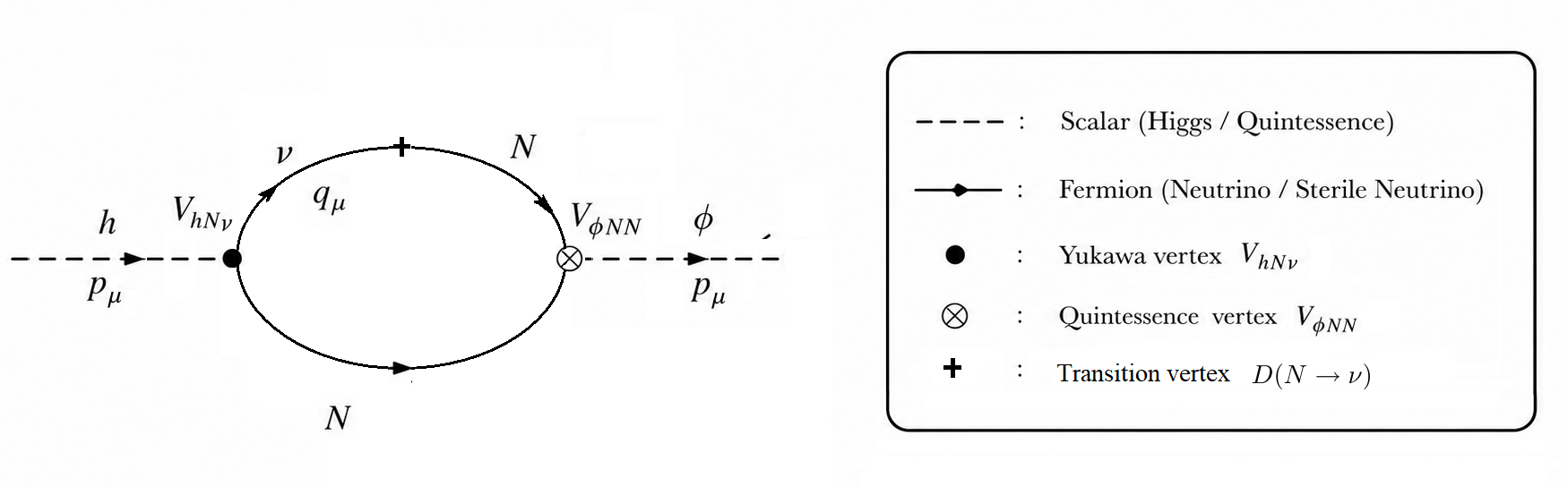
This polarization loop (self-energy), which mixes the scalar fields, has the following form:
Using Feynman parametrization, the integral can be rewritten as
| (27) |
This expression is finite. Integrating over momentum gives
| (28) |
The final part of the integral can be evaluated, but the expression is not simple. Instead, we can estimate useful limits to obtain asymptotic behavior:
| (29) | ||||
| (30) |
Correspondingly, the polarization function becomes
| (31) | ||||
| (32) |
with
| (33) |
has the same structure whether the Higgs oscillates into quintessence or vice versa, when expressed in terms of and with out apprixmations. From the form of , we conclude that depending on the process one can encounter either kinetic mixing, mass mixing, or a mixed case. For on shell processes, is naturally associated with the corresponding mass scales or , while for off shell effects, a wide variety of possible values can arise. Thus, we can distinguish three scenarios:
1. Heavy sterile neutrino case: and . At TeV scales and below, regardless of the hierarchy between quintessence and Higgs masses, the mixing is of kinetic type.
2. Light sterile neutrino case: and . This corresponds to a clear example of mass type mixing, but is only realizable for very heavy quintessence scenarios.
3. Intermediate or near-degenerate case: When the mass scales are close to one another, or the sterile neutrino is lighter than the Higgs but heavier than quintessence, or when the propagating momentum satisfies , the full expression must be retained and mixing effects evaluated case-by-case at the Feynman diagram level.
Let us note that the suppression structure appearing in this loop induced mixing effect is the same as in the Higgs tree level decay process considered above.
4.1 The kinetic mixing
For the case , kinetic mixing remains uniform at and below the electroweak scale. In this regime, it is straightforward to incorporate the corresponding mixing operator into the Lagrangian:
| (34) |
Diagonalization can then be attempted by identifying mass states. The linear transformation
| (35) |
diagonalizes the scalar states. This procedure is equivalent to performing an orthogonal transformation between the Higgs and quintessence scalars, normalizing the kinetic structure, and then diagonalizing the mass matrix by another orthogonal transformation. However, the transformation is given only to linear order in . In this limit, the mass values remain unchanged. Calculating effects at order would not be consistent, since two loop contributions are expected to be of the same order.
Physically, this mixing corresponds to on-shell quintessence or Higgs bosons oscillating into their counterpart and then decaying into whatever channels are kinematically allowed. Such mixing allows quintessence to interact with SM particles – lepton–antilepton pairs, quark–antiquark pairs, and massive gauge bosons similar to the Higgs itself, but with reduced strength defined by the transformation above. Some of this three particle interaction verteces are:
| (36) | ||||
| (37) | ||||
| (38) |
Here, are the Yukawa couplings of leptons and quarks to the Higgs, while and are masses of and charged -bosons. Although these couplings are strongly suppressed and none of them open direct kinematic decay channels for a light quintessence field, the analogy with the Higgs suggests that radiative decay into two photons remains the only guaranteed possibility. This process, together with other potential quintessence decay channels, may be relevant for cosmological signatures: a quintessence condensate could undergo perturbative decay, emit photons of characteristic energy, and thereby alter the dynamics of dark energy.
Finally, if the masses of quintessence and the Higgs are correlated by some yet unknown physics, and a certain level of fine-tuning occurs between them, the mixing effect could be significantly amplified, increasing the likelihood of detection.
4.1.1
Fig. 3 below illustrates how this process proceeds.

To calculate its matrix element, we first recall the form of the -lepton-antilepton vertex:
| (39) |
where is the electric charge, is Weinberg angle and for neutrinoes, while for electrons, muons, and tau leptons. In the leading order, lepton masses can be neglected.
Employing (37), the matrix element becomes
| (40) |
where is the Z-boson propagator in unitary gauge carrying momentum . Using on-shell conditions, this simplifies to
| (41) |
Squaring the amplitude and averaging over Z-boson polarizations yields
| (42) |
The Dirac traces evaluate to
Thus,
| (43) |
Using momentum conservation and taking the Z-boson in its rest frame simplifies the expression to
| (44) |
The differential decay rate is then
| (45) |
Integration over phase space proceeds analogously to the Higgs decay case discussed earlier. Here, however, resonance does not occur. As before, we can neglect the quintessence mass, since small maximizes the weak boson decay rate (excluding effect because of mixing ratio (35), as it mentioned above fine-tuned values of and may leave perturabative limit for the mixing). In the limit of small , in the leading order we obtain
| (46) |
Relative to the Standard Model Z-boson decay rate into a specific lepton channel, , the ratio is
| (47) |
This ratio is proportional to the square of the mixing parameter (35).
A similar result holds for analogous three-particle decay processes of the charged weak boson and the Higgs boson (madiated by the (38)). In all cases, the suppression factor is too severe to have any meaningful impact on accelerator or cosmic ray physics.
4.1.2 The Higgs decay via quintessence self interaction
Apart from decay processes fostered by Standard Model interactions, depending on the model one may also encounter three point self-interactions of the quintessence field. Through mixing, such interactions generate the possibility of Higgs decay into two quintessence particles in light quintessence scenarios:
| (48) |
This scalar process is straightforward. In the Higgs rest frame, the decay rate into the quintessence channel can be written as
| (49) | ||||
| (50) |
where and are the outgoing quintessence momenta and . Taking (33) into account, and assuming an eV, we obtain
| (51) |
This necessarily pushes to scales higher than eV in order for the decay rate to remain at least in the eV range. Such a requirement corresponds to an extremely strong coupling. For reference, in inflessence models where mass and coupling are defined as
| (52) |
with the Planck mass and the inflation scale, such a large value of pushes the inflation scale up to the GUT regime and the inflessence mass also near the GUT scale. Consequently, this decay becomes impossible in inflessence scenarios where the coupling is strong enough. Beyond inflessence models, quintessence potentials and self-couplings are typically feeble.
4.1.3 Quintessence decay
From the decay processes of massive bosons discussed earlier, it is clear that the tiny contributions to SM particle decay rates play no practical role. However, the situation for the quintessence field is different. Quintessence is supposed to be sufficiently stable to fulfill the role of dark energy, and even very small decay rates can have significant consequences for its cosmological evolution. If we denote the quintessence decay rate by , then the evolution of the field energy density in coupled models can be modeled by
| (53) |
where is the Hubble constant and is the equation of state parameter. In the slow-roll regime, even if remains close to and if (with the current Hubble constant), the energy density decays exponentially:
| (54) |
Depending on how close is to minus one and how large is, quintessence decay can be unacceptably fast for DE modeling. In any case, provides a natural reference scale for constraining . Models in which quintessence does not sit at the absolute minimum of its potential, and achieves slow roll differently, cannot afford . In the recent work [21] it is even claimed that few order of magnitude smaller then is to explain DESI results and phantom crossing. So, may be smaller is even preferable.
. One loop mixing effects open the possibility for quintessence decay into an electron–positron pair if . With mixing already taken into account, this is a simple tree-level process with coupling strength (36). The squared matrix element is
| (55) |
where and are the electron and positron four momenta. Momentum conservation gives , so
| (56) |
In the rest frame, the decay rate is
| (57) | ||||
| (58) |
From this clean expression, assuming MeV, we estimate
| (59) |
which implies the constraint
| (60) |
This becomes meaningful only if GeV, since GeV.
. Quintessence can always decay radiatively into two photons, analogous to the Higgs decay into two photons. The Higgs decay rate is well known [22],
| (61) |
where is the Fermi constant, the fine-structure constant, the color factor, the fermion charge, and , with . The loop functions are:
| (62) | ||||
| (63) |
with
| (64) | ||||
| (65) |
To obtain , quintessence decay rate, we should replace with where is a need and adjust couplings. We note that typically is light compared to heavy fermions and W bosons, so and . This gives the approximations
| (66) |
For very light quintessence, all fermions contribute similarly. If four momentum of the quintessence is
| (67) | ||||
| (68) |
Since , for the rest frame quintessence decay rate we should have
| (69) |
Comparing this to the Hubble constant, we find
| (70) |
Since is at leasy , being proportional to the ratio of the active neutrino mass to the electroweak scale, this constraint may become cosmologically relevant if . For , lighter fermions no longer contribute significantly, but the overall magnitude of the decay rate remains unchanged.
Here we compared the tiny decay rate of quintessence to . However, if values below are preferred [21], the (, ) parameter space becomes more narrow.
5 The mass mixing
When the mixing term is introduced as
| (71) |
an orthogonal transformation linear in
| (72) |
diagonalizes the scalar states. Here the transformation parameter depends explicitly on the sterile neutrino mass . Since in this case the sterile neutrino is comparatively light, the mixing is additionally suppressed. The contribution to the diagonal mass values is again a second order effect, proportional to . New interactions appear in analogy to the kinetic mixing case, but are further suppressed by the ratio of the sterile neutrino mass to the heavier of the Higgs and quintessence masses.
Unlike the kinetic mixing scenario, processes requiring light quintessence (such as weak and Higgs boson decays considered above) do not occur here. However, quintessence decay processes are amplified by the large quintessence mass.
Quintessence decay into . The decay rate into an electron–positron pair is modified directly from (58) by replacing
| (73) |
This modifies the restriction to
numerically yelding
| (74) | ||||
| (75) |
This sets a constraint on the Yukawa coupling which is of order unity for TeV, GeV. This is essentially equivalent to the limit derived in the previous subsection. For heavier quintessence, the constraint becomes considerably relaxed. In any case, this is not a primary decay channel for quintessence. Compared to the dominant sterile neutrino decay rate (5), it is completely negligible – unlike the light quintessence scenarios, where the sterile neutrino decay channel is kinematically forbidden.
| (76) |
Quintessence decay into photons. For the decay channel into photons, when quintessence is assumed to be much heavier than the Higgs, the loop contributions simplify:
The decay rate is then estimated as
| (77) |
This decay rate is also strongly suppressed compared to (5) and appears unimportant.
6 Momentum-dependent mixing
When the parameter space or energy scale of the process does not allow a blanket diagonalization of the scalar fields, the off diagonal self-energy depends nontrivially on momentum. In such cases, a single momentum independent diagonalization of the fields is not possible, and one must instead account for the effects of directly at the Feynman diagram level.
For example, consider an on-shell Higgs decaying through oscillation into quintessence, followed by quintessence decaying into some final state . The matrix element for the decay rate in the rest frame is
| (78) |
- •
- •
When the situation is reversed — quintessence decaying through oscillation into the Higgs, followed by Higgs decay into some final state – the amplitude is
| (81) |
again reproducing either kinetic or mass mixing behavior depending on the hierarchy of scales.
Because of possible hierarchies between mass scales, we can encounter mixed behavior. When there is no clear hierarchy, or when the propagating momentum is off-shell, the full expression must be retained and evaluated case-by-case.
This non-uniform regime does not introduce fundamentally new phenomena; it simply interpolates between the properties of mass mixing and kinetic mixing depending on the process. The approach described here is universally valid but requires case-by-case consideration, whereas the pure mass mixing or kinetic mixing limits offer more simplicity and uniformity when the parameter space allows them.
7 Conclusion
We investigated the consequences of coupling a quintessence field to sterile neutrinos in a seesaw framework. While the interaction between quintessence and sterile neutrinos is introduced at tree level, the presence of the standard Higgs–sterile-neutrino Yukawa interaction inevitably generates Higgs – quintessence mixing through radiative corrections. This effect provides a portal through which quintessence acquires effective interactions with Standard Model particles.
The one-loop mixing amplitude was calculated and analysed in different momentum regimes. We find that the nature of the mixing depends on the relation between the characteristic momentum transfer and the sterile-neutrino mass. For the mixing assumes a kinetic form and can be represented by an effective derivative operator between the Higgs and quintessence fields. In contrast, for the mixing behaves as a mass-type contribution. Between these limits the mixing remains momentum dependent and cannot generally be removed by a single field redefinition. The induced Higgs–quintessence mixing generates effective couplings of quintessence to fermions and gauge bosons. As a result, processes involving Higgs, and bosons receive additional contributions through intermediate quintessence states. The corresponding corrections are strongly suppressed by neutrino masses and by loop factors and are therefore expected to remain below current experimental sensitivities in the minimal scenario considered here.
The same mixing mechanism opens decay channels for quintessence. For sufficiently heavy quintessence fields, decays into charged fermions become possible, while radiative decay into two photons remains available even for very light quintessence. Although these processes are highly suppressed, the extreme longevity required of a dark-energy field makes even tiny decay rates potentially relevant from a cosmological perspective. The resulting constraints provide a complementary way of probing interactions between quintessence and sterile neutrinos.
The suppression obtained in the present work is largely a consequence of the heavy-seesaw limit. In models containing several sterile neutrino states, lighter sterile neutrinos may contribute significantly to loop processes and modify the phenomenology. In such cases the momentum dependence of the mixing and threshold effects can become considerably more important, potentially enhancing observable signatures.
Overall, the results demonstrate that sterile-neutrino-assisted quintessence models naturally predict Higgs–quintessence mixing and consequently a broad class of effective interactions between quintessence and Standard Model fields. While the effects appear small in the simplest heavy-seesaw realization, the framework establishes a direct connection between dark-energy dynamics, neutrino mass generation and collider-scale particle physics.
Acknowledgments
I would like to thank Jon Chkareuli and Michael Maziashvili for useful and fruitful discussions.
References
- [1] P.J.E.Peebles, B.Ratra. Cosmology with a Time Variable Cosmological Constant. Astrophys. J.Lett.325, L17(1988). DOI: 10.1086/185100. B.Ratra, P.J.E.Peebles. Cosmological Consequences of a Rolling Homogeneous Scalar Field. Phys.Rev.D37, 3406(1988). https://doi.org/10.1103/PhysRevD.37.3406
- [2] I. Zlatev, L.M.Wang, P.J.Steinhardt. Quintessence, cosmic coincidence, and the cosmological constant. Phys.Rev.Lett.82,896(1999). https://doi.org/10.1103/PhysRevLett.82.896 P.J.Steinhardt, L.M.Wang, I.Zlatev. Cosmological tracking solutions. Phys.Rev.D59,123504(1999). https://doi.org/10.1103/PhysRevD.59.123504
- [3] P.Binetruy. Models of dynamical supersymmetry breaking and quintessence. Phys.Rev.D60,063502(1999). https://doi.org/10.48550/arXiv.hep-ph/9810553
- [4] P.Brax, J.Martin. The Robustness of quintessence. Phys.Rev.D61,103502(2000). https://doi.org/10.48550/arXiv.astro-ph/9912046
- [5] S.Dutta, R.J.Scherrer. Hilltop Quintessence. Phys. Rev. D 78, 123525 (2008). https://doi.org/10.48550/arXiv.0809.4441
- [6] A.Gonzalez, T.Matos, I.Quiros. Unified Models of Inflation and Quintessence. Phys.Rev. D71 (2005) 084029. https://doi.org/10.48550/arXiv.hep-th/0410069
- [7] L.A.Salo, J.Haro. Quintessential Inflation for Exponential Type Potentials: Scaling and Tracker Behavior. Eur. Phys. J. C 81, 105 (2021). https://doi.org/10.48550/arXiv.2009.12912
- [8] S.C.Park. Non-minimally coupled quintessential inflation. Progress of Theoretical and Experimental Physics, Volume 2025, Issue 10, October 2025, 103E02. https://doi.org/10.48550/arXiv.2412.08833
- [9] R.Fardon, A.E.Nelson, N.Weiner. Dark Energy from Mass Varying Neutrinos. JCAP 0410:005,2004. https://doi.org/10.48550/arXiv.astro-ph/0309800
- [10] A.W.Brookfield, C.van de Bruck, D.F.Mota, D.Tocchini-Valentini. Cosmology with massive neutrinos coupled to dark energy. Phys. Rev. Lett. 96, 061301 (2006). https://doi.org/10.48550/arXiv.astro-ph/0503349 A.W.Brookfield, C.van de Bruck, D.F.Mota, D.Tocchini-Valentini. Cosmology of mass-varying neutrinos driven by quintessence: theory and observations. Phys. Rev. D73, 083515 (2006), Phys. Rev. D76, 049901 (2007). https://doi.org/10.48550/arXiv.astro-ph/0512367
- [11] Ole Eggers Bjælde et al. Neutrino dark energy—revisiting the stability issue. JCAP01(2008)026. https://doi.org/10.48550/arXiv.0705.2018
- [12] M.Maziashvili, V.Tsintsabadze. Avoiding parameter fine-tuning in mass varying neutrino models of DE? Astropart. Phys. 154, 102901 (2024). https://doi.org/10.48550/arXiv.2302.00380
- [13] Z.Kepuladze, M.Maziashvili. A new take on the inflationary quintessence. Phys. Rev. D103, 063540 (2021). https://doi.org/10.48550/arXiv.2102.09203
- [14] Z.Kepuladze. Quantum dark energy from neutrino loops: model, stability and oscillation imprints. Eur.Phys.J.C 85 (2025) 12, 1423. : 10.1140/epjc/s10052-025-15150-5. https://doi.org/10.1140/epjc/s10052-025-15150-5
- [15] Z.Kepuladze. Radiative dark energy in a seesaw framework. Phys.Lett.B 876 (2026) 140422. https://doi.org/10.1016/j.physletb.2026.140422
- [16] K.Kaneta, Hye-Sung Lee, J.Lee, J.Yi. Gauged Quintessence. JCAP02(2023)005. https://doi.org/10.48550/arXiv.2208.09229
- [17] R.Barbieri, L.J.Hall, Steven J. Oliver, A.Strumia. Dark Energy and Right-Handed Neutrinos. Phys.Lett.B625:189-195,2005. https://doi.org/10.48550/arXiv.hep-ph/0505124
- [18] K.S.Babu, G.Chauhan, P.S.Bhupal Dev. Neutrino Non-Standard Interactions via Light Scalars in the Earth, Sun, Supernovae and the Early Universe. Phys. Rev. D 101, 095029 (2020). https://doi.org/10.48550/arXiv.1912.13488
- [19] G.D’Amico, T.Hamill, N.Kaloper. Neutrino Masses from Outer Space. Phys.Lett.B 797 (2019) 134846. https://doi.org/10.48550/arXiv.1804.01542
- [20] V.Brdar, M.Lindner, S.Vogl, Xun-Jie Xu. Revisiting Neutrino Self-Interaction Constraints from and decays. Phys. Rev. D 101, 115001 (2020). https://doi.org/10.48550/arXiv.2003.05339
- [21] Prolay Chanda, Subinoy Das, Suratna Das. Dissipative Dark Energy can explain the DESI phantom crossing. Arxiv Preprint: https://doi.org/10.48550/arXiv.2606.04886
- [22] Abdelhak Djouadi (LPTO). The Anatomy of Electro-Weak Symmetry Breaking. I: The Higgs boson in the Standard Model. Phys.Rept.457:1-216,2008. https://doi.org/10.48550/arXiv.hep-ph/0503172