Interference Queueing Networks: A Replica Mean-Field Approach in the Symmetric Setting

Philippe Sarotte, Nahuel Soprano-Loto¹¹footnotemark: 1, François Baccelli¹¹footnotemark: 1 INRIA, Paris

Abstract

We propose a model for evaluating the performance of wireless communication networks beyond the ubiquitous full-buffer assumption, under which every transmitter is always active. The network is represented by $N$ interacting queues arranged on a torus, with homogeneous arrival rate $\lambda$ and service rates depending on the activity of neighboring interferers. More precisely, each queue is associated with a transmitter–receiver pair, and its service rate is given by the Shannon capacity, which depends on the corresponding Signal-to-Interference-plus-Noise Ratio (SINR). Since interfering transmitters only emit when their queue is non-empty, the SINR – and hence the service rate – improves when neighboring queues are empty. We first derive the stability region of the system. To investigate the stationary regime, we introduce two mean-field approximations. The first one is obtained from a finite $K$ -replica system, for which we prove propagation of chaos as $K\to\infty$ . The second one describes a queueing system evolving in a suitably chosen autonomous environment. We derive quantitative estimates comparing these two approximations. Finally, we prove that the original interacting queueing system converges exponentially fast to stationarity.

Index Terms—Spectrum sharing, queueing networks, wireless interference, mean-field approximation, McKean–Vlasov dynamics, performance analysis, coupling

1 Introduction

1.1 Motivation

The goal of this paper is to introduce a tractable model for analysing the performance of wireless networks operating over a shared bandwidth beyond the classical full-buffer assumption. Rather than assuming that all transmitters are perpetually backlogged, we consider a system with bursty traffic, where packets arrive dynamically and are stored in queues before transmission. The resulting interaction between traffic dynamics and interference leads to a coupled queueing system whose analysis is challenging. Beyond its theoretical interest, this finer-grained analysis can provide useful guidance for network dimensioning and engineering. By explicitly accounting for the interaction between packet arrivals, queue occupancy, and interference, it becomes possible to assess more accurately the admissible load, the density of simultaneously active links, and the conditions under which full spectrum sharing remains viable. This, in turn, can inform the design of current wireless networks by indicating when mechanisms such as admission control, power control, or partial spectrum partitioning are needed to avoid persistent congestion.

We model the network as a collection of transmitter–receiver pairs sharing the same wireless medium. Each transmitter stores packets arriving at a rate $\lambda$ in a queue and serves them over its associated wireless link. When several neighbouring transmitters are simultaneously active, they interfere with one another, so that the transmission rate of each active link depends on the current activity of the surrounding queues. Under adaptive coding and ideal Gaussian signalling, this dependence is captured through the Shannon capacity formula, which links the service rate of each queue to the instantaneous signal-to-interference-plus-noise ratio. The service process is therefore state-dependent, and all queues become coupled through interference. Our aim in this paper is to study the fundamental queue–interference coupling within a mathematically tractable framework, at the expense of several simplifying assumptions. These assumptions are admittedly restrictive, but they allow us to introduce the main phenomena and develop mathematical tools that can later be extended to more realistic settings. We now summarise them.

•

One queue per wireless link. Each queue corresponds to a transmitter–receiver pair, with each transmitter serving at most one receiver at a time.
•

Short links. Receiver–transmitter distances are assumed small compared with inter-transmitter distances, i.e., $T\ll d(i,j)$ . Hence, the interference at a receiver is approximated by that at its transmitter.
•

Homogeneous queues. All queues are statistically identical, with common arrival rate, file-size distribution, transmit power, link distance, and fading statistics.
•

Interference-dependent service. A queue service rate depends on the set of simultaneously active transmitters through interference, according to the Shannon capacity formula.
•

Full frequency reuse. All links share the same frequency band, so interference is not mitigated by orthogonal resource allocation.
•

Symmetric geometry. Transmitters are equally spaced on a torus, ensuring identical interference conditions for all nodes and eliminating edge effects. Periodic boundary conditions should be understood as a proxy for a finite window within a larger homogeneous network.
•

Static channel model. We consider a quasi-static channel with constant noise over the time interval of interest. Under translation invariance, links with the same relative geometry have identical fading statistics, and instantaneous fading is replaced by its mean power in the SINR.
•

Ideal rate adaptation. Rate adaptation is assumed instantaneous and overhead-free, so transmission always operates at the Shannon capacity corresponding to the current interference state.

Within this setting, several natural performance questions arise. Can the stability region of the system be characterised explicitly? When the system is stable, can one describe its stationary regime and derive performance metrics such as mean delay or congestion? Can the analysis be extended to random spatial configurations? Finally, what can be said about the long-time behaviour of the system and its convergence to equilibrium?

1.2 Related Work

Stochastic analysis has long been central to the performance evaluation of telecommunication networks, providing mathematically grounded approximations and scaling laws that help identify key design parameters without costly deployment campaigns or extensive measurements; see, e.g., [2].

Several works have relaxed the full-buffer assumption in wireless settings. In [28], a device-to-device model is introduced in which files are transmitted at the Shannon rate in a bounded continuous space with randomly located transmitters. A related model on an infinite countable space with deterministic transmitter locations is studied in [27]. For cellular downlink systems, [1] considers the single-cell case, while [22], [32], [8], and [7] study multi-cell models with randomly located users and explicit multiple-access mechanisms.

A major challenge in the analysis of such systems is the presence of spatial and temporal correlations between particles, which typically make an exact treatment intractable. A natural approach is therefore to approximate the original dynamics by a mean-field limit; see, e.g., [22, 25]. While mean-field limits provide a powerful analytical framework, proving the existence of the limiting model may itself be delicate, as the limits in time and in the number of particles do not necessarily commute. This phenomenon appears, for instance, in the Kuramoto model [6] and in the Curie–Weiss model [21]. The long-time behaviour of either the finite system or its mean-field approximation has been investigated in various settings, such as [19], where the limiting dynamics are governed by an ODE, and [12], where the McKean–Vlasov nonlinearity enters through the drift.

1.3 Contributions

We now summarize the main contributions of the paper, their interpretation in plain terms, the main technical obstacles encountered in the analysis, and their relevance for performance evaluation.

As described in the motivation section, the system consists of interacting queues receiving jobs at rate $\lambda$ and transmitting them at rates that depend on the activity of the whole network. More congested systems have smaller transmission rates. This creates a natural competition between the arrival mechanism, which tends to increase the workload, and the service mechanism, which allows the system to empty itself.

Our first contribution is to make this intuition rigorous. We prove the existence of a critical threshold for the arrival rate. Below this threshold, the system is stable, in the sense that it returns to the empty state infinitely often. Above it, with probability $1$ the number of jobs diverges to infinity. This threshold has a natural interpretation: the arrival rate must be smaller than the worst-case transmission rate $\mu^{*}$ , corresponding to the rate at which a queue transmits when all surrounding queues are active. We also realize that it means that taking into account the empty slots does not enlarge the stability region of the queuing system.

To establish this result, we first provide a stochastic differential equation representation of the system, in a form reminiscent of interacting neuron models. This formulation makes it possible to construct explicit couplings by using the same Poisson random measures. In the regime $\lambda<\mu^{*}$ , stability follows from stochastic domination by the full-buffer system, whose explosion region is known. The converse direction is more delicate, since a direct stochastic domination argument is no longer available. Instead of relying on Lyapunov methods or fluid-limit techniques at this stage, we use coupling arguments that exploit the fact that the true system behaves like the full-buffer system whenever no queue is empty.

We then turn to the stable regime and to the problem of estimating stationary performance metrics, such as delay, congestion, and busy probability. Obtaining closed-form expressions, or even sampling from the exact stationary distribution, is a notoriously difficult problem. In the present setting, the difficulty is closely related to the analysis of random walks in the positive orthant with boundary interactions. Existing results, in particular those of [14], indicate that an exact description is in general out of reach. We therefore adopt an approximation approach.

The purpose of our approximations is to remove the main source of analytical difficulty, namely the randomness of the transmission rates induced by the current state of the other queues. Mean-field approximations achieve this by replacing this random quantity with a simpler averaged one. This reduction leads to tractable objects, essentially of $M/M/1$ type, for which stationary performance metrics can be computed. A further difficulty, however, is that the approximation should still preserve the geometry of the original system, in particular the notion of distance between queues. To this end, we introduce a replica-type mean-field construction.

More precisely, we define a replica-type prelimit system and prove propagation of chaos towards a limiting system in which the random interaction term is replaced by its averaged counterpart. This gives a rigorous interpretation of the approximation as the limit of a finite interacting system. The proof relies on classical Sznitman coupling techniques, adapted to Poisson random measures, in the spirit of mean-field limits for interacting neuron systems. In this way, the difficulty associated with random service rates in the original system is transferred to the McKean–Vlasov nonlinearity of the limiting system. Nevertheless, in stationarity, the limiting queues recover an $M/M/1$ -type structure, which makes the approximation analytically tractable. We also observe that the well-posedness region of the approximation coincides with the stability region of the true system. This agreement further supports the relevance of the approximation.

We also introduce a second mean-field approximation. In this case, we do not address the question of identifying a prelimit system from which it arises. Instead, we focus on replacing the random transmission rate by an independent copy with the same distributional structure. This leads to a different class of tractable models, namely queues in a random autonomous environment. We use known stability and stochastic-ordering results for such systems, in particular convex-order comparisons with respect to the averaged environment. Using functional inequalities and the convexity properties of the Shannon rate, we obtain qualitative comparisons between the two mean-field approximations through Jensen-type arguments.

The analytical results are then compared with numerical simulations. The simulations confirm the theoretical predictions and highlight a significant difference between the full-buffer system and the true system. This confirms the need for a refined analysis that accounts for empty queues. The numerical results also show that the two mean-field approximations capture different aspects of the system: the first approximation performs well for the mean delay and congestion, whereas the second approximation is more accurate for the busy probability. Moreover, as the impact of interference decreases, the discrepancies between the different systems become smaller.

We further study the long-time behaviour of the true system. To do this, we prove a Foster–Lyapunov drift condition and then use exponential ergodicity criterion. This result is relevant for numerical implementation, since it justifies that stationary samples can be obtained without simulating the system over excessively long time horizons.

Finally, we extend the analysis to systems with randomly spaced queues. This extension emphasizes that our approximations preserve the underlying geometry of the network and that the mean-field results can still be applied in this more general spatial setting.

1.4 Structure of the paper

The remainder of the paper is organized as follows. Section˜2 introduces the main physical concepts underlying the analysis, fixes the notation, and presents the model in two equivalent formulations: through its Markovian description and through its SDE representation. The latter point of view will play an important role throughout the paper. Section˜3 states the main results, first in a mathematically rigorous form and then in a more intuitive formulation. More precisely, Section˜3.1 describes the stability region, while Section˜3.2 studies the stationary distribution and its approximation by two McKean–Vlasov systems. One of these systems arises as the limit of a system of replicas, for which propagation of chaos is established. Next, Section˜3.3 investigates the long-time behavior of the original system. Section˜3.4 then considers random transmitter positions, which, in the symmetric case, amounts to random common spacings. The proofs of the results are given in Section˜4, in the same order as their presentation. Section˜5 discusses several extensions that will be addressed in subsequent papers. Finally, Appendix˜A collects auxiliary results and proofs, included either for completeness or to avoid interrupting the flow of the main text.

2 Setting, notation, and assumptions

2.1 Assumption on the Physical Model

As mentioned in the introduction, our model applies to almost any network sharing a common bandwidth, in which each transmitter serves only one receiver at a time and the distances between transmitters are relatively large compared with those between transmitters and receivers. As already acknowledged, one may argue that this framework is not fully realistic, especially given the additional assumptions of homogeneous arrival rates, equally spaced transmitters, assuming the availability of capacity-achieving codebooks across different channel conditions and density of the interaction graph neglecting frequency reuse. However, we emphasize that this paper is the first in a sequence of works whose purpose is to progressively relax these assumptions in order to better reflect reality. The goal here is to introduce the main ideas and mathematical tools in the simplest possible setting, so that the exposition remains clear.

2.2 Key Physical quantities

Here we describe precisely the main quantities of the model, namely the Signal to interference Noise ratio (SINR) and the Shannon rate.

2.2.1 SINR

The Signal to Interference Noise ratio is a key quantity to understand whether signal can be transmitted reliably at a given rate. For a scenario where a transmitter located at position $0$ sends a message to a receiver at position $x$ in the presence of other transmitters, having a message to send, located in the atomic set $S$ , we will use the following definition:

\displaystyle\mathrm{SINR}(x)=\frac{P_{e}\,h_{0}\,l(0,x)}{W+\sum_{y\in S}P_{e}\,h_{y}\,l(y,x)}.

1.

The transmissions power is $P_{e}$ . In this framework, all transmitters are assumed to operate at the same constant power.
2.

The fading coefficient is denoted by $h_{y}$ for the $y$ -th transmitter. This term models channel fluctuations due to multi path in a simplified manner without solving the full electromagnetic wave equations. Typically, $h_{y}$ is a random variable following a specific distribution, for example, Rayleigh, see [2]. Here we assume it is constant.

The path loss function is $l(x,y)$ . It accounts for the reduction in signal power with distance. The further away the receiver is from the transmitter, the weaker the received signal. Common models include power-law functions, which may or may not exhibit a singularity at $0$ . In this paper, we consider a family of path-loss functions belonging to the following set:

\mathcal{L}(A,C,r_{0})\;=\;\left\{\begin{aligned} &\ell_{1}(r)=\frac{1}{\bigl(A\cdot\max(r,r_{0})\bigr)^{C}},\\[6.00006pt] &\ell_{2}(r)=\frac{1}{\bigl(1+Ar\bigr)^{C}},\\[6.00006pt] &\ell_{3}(r)=A\,e^{-Cr}\end{aligned}\;\middle|\;A>0,\;C>0,\;r_{0}>0\right\}.

4.

$W$ represents the power of the noise aside from interference, such as thermal noise. It can be modeled by a non negative random variable independent of the rest of the system. Here we assume it is constant.

For the sake of readability, we henceforth set all constants equal to one. This does entail a loss of generality at the level of the model, but the analysis extends to arbitrary constants with only notational modifications.

2.2.2 Shannon Rate

The Shannon rate is another fundamental concept in telecommunications and information theory. When transmitting a message, one encodes it into symbols which are transmitted over a channel subject to perturbations before being decoded at the receiver. The goal is to design an encoding and decoding scheme such that the original message is recovered with probability arbitrarily close to one. In a basic, non-adaptive transmission scheme, successful transmission occurs if the SINR exceeds a certain threshold. However, when one has multiple codes that can be dynamically adapted to changing channel conditions, [29] showed that when treating interference as noise, the maximum achievable rate of reliable information transmission is given by the Shannon capacity:

\displaystyle C=B\log_{2}\bigl(1+\mathrm{SINR}\bigr),

where $B$ denotes the bandwidth used by the network. In our framework, we assume that we have coding schemes capable of matching any channel condition. We further assume that adaptation to channel conditions is instantaneous, and therefore ignore any delay induced by the adaptation mechanism.

2.3 Description of the system and notation

2.3.1 Markovian Description

We consider a system of $N$ queues equally spaced on the torus $[0,N-1]$ , where each job represents a file to be transmitted (see Figure˜1). The state of the system is described by the congestion process

\displaystyle Q(t)=\bigl(q_{1}(t),\dots,q_{N}(t)\bigr),

(1)

where $q_{i}(t)$ denotes the number of jobs present in queue $i$ at time $t$ .

Refer to caption — Figure 1: Mathematical representation of the symetric wireless network

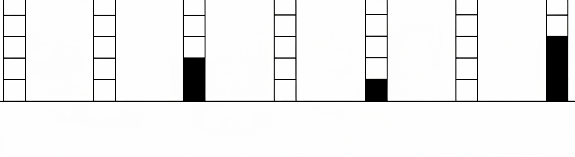
We place ourselves in a Markov framework, hence $Q$ is a (non explosive) continuous time Markov chain with respect to its natural filtration and can be described thanks to its generator: For any bounded $f$ from $\mathbb{R}^{N}$ to $\mathbb{R}$ :

\displaystyle\mathcal{L}f(q)=\lambda\sum_{i}\big(f(q+e_{i})-f(q)\big)\;-\;\sum_{i}\mu_{i}(q)\,\big(f(q)-f(q-e_{i})\big)\,\mathbf{1}_{\{q_{i}>0\}},

(2)

where

•

$\mu_{i}(q)=\frac{B}{L}\log_{2}\!\left(1+\frac{1}{1+\sum_{j\neq i}\mathbf{1}_{\{q_{j}>0\}}\,l(d(i,j))}\right).$
•

The vector $e_{i}$ is only 0 except at position $i$ there is a $1$ .
•

$l\in\mathcal{L}(A,C,r_{0})$ ,
•

The circular distance between the i-th buffer and the j-th one is denoted by $d(i,j)$ .
•

We define $\xi_{N}:=\sum_{j\neq i}l(d(i,j))$ , which refers to the worst interference conditions, that is, all neighboring queues are non-empty. Note that it is a common quantity for each queues in our equally spaced, periodic boundary conditions.
•

In the same fashion we define $\mu^{*}:=\frac{B}{L}\log_{2}\!\left(1+\frac{1}{1+\xi_{N}}\right)$ and $\mu^{**}:=\frac{B}{L}$ as being the worst and best service rates.

In essence, the system operates as follows:

•

Job arrivals at each queue form independent Poisson processes with rate $\lambda$ .
•

Job sizes are i.i.d. exponential random variables with parameter (mean) $L$ , independent of the arrival processes. We will take $L=1$ to simplify notations.
•

The instantaneous transmission rate of queue $i$ at time $t$ is denoted by $\mu_{i}(t)$ .

Remark 2.1.

The full-buffer system is obtained by replacing each $\mathbf{1}_{\{q_{j}>0\}}$ with $1$ . In this case, the system reduces to $N$ independent $M/M/1$ queues.

Remark 2.2.

We used the Shannon rate for the departure rate but actually we can broaden the analysis to any $g:[0;\xi_{N}]\to\mathbb{R}^{+}$ , being bounded, non increasing, convex, smooth enough (mainly Lipschitz) and $\mu_{i}(t)=\frac{1}{L}g(\sum_{j\neq i}\mathbf{1}_{\{q_{j}(t)>0\}}\,l(d(i,j)))$ . Doing so, all the following results still hold. The Shannon rate description is retrieved by taking $g(x)=B\log_{2}(1+\frac{1}{1+x})$ .

Remark 2.3.

Thanks to the periodic boundary condition and the equal spacing of the queues, they have the same marginals.

2.3.2 Dynamical description

Here we describe the system in terms of SDE with respect to Poisson random measures which is, as we mentioned, crucial in our analysis . We will see that those two representations are equivalent in law thanks to Martingale problem considerations. Consider $(A_{i})_{i\in[0;N-1]}$ , $N$ i.i.d. Poisson point processes of intensity $\lambda\rm{d}x$ . In addition consider $(D_{i})_{i\in[0;N-1]}$ i.i.d. Poisson point processes of intensity $\rm{d}xdy$ . Now define $\tilde{Q}=(\tilde{q}_{1},\dots,\tilde{q}_{N})$ as

\displaystyle\widetilde{q}_{i}(t)

\displaystyle=\widetilde{q}_{i}(0)+A_{i}[0,t]-\int_{0}^{t}\int_{\mathbb{R}_{+}}\mathbf{1}_{\{\widetilde{q}_{i}(z^{-})>0\}}\mathbf{1}_{\{u\leq\mu_{i}(\widetilde{Q}(z^{-}))\}}\,D_{i}(\mathrm{d}u,\mathrm{d}z),\qquad i=0,\dots,N-1.

(3)

Remark 2.4.

(3) is well defined and represents the same object in law as (1). See Appendix˜A for the proofs.

2.3.3 Notation

•

For $x,y\in\mathbb{N}^{N}$ , we denote by $x\leq y$ the partial order on $\mathbb{N}^{N}$ defined component-wise, that is,

$x\leq y\quad\text{if and only if}\quad x_{i}\leq y_{i}\text{ for all }i\in\{1,\dots,N\}.$
•

For two $\mathbb{N}^{N}$ -valued random variables $X$ and $Y$ , we write $X\leq_{\mathrm{st}}Y$ whenever $X$ is stochastically dominated by $Y$ .
•

For two $\mathbb{N}^{N}$ -valued random variables $X$ and $Y$ , we write $X\leq_{\mathrm{icx}}Y$ whenever $X$ is greater than $Y$ for the increasing convex ordering, see [3] for more details.

3 Main Results

3.1 Stability Region

In this section, we state the stability region of the system. Since $Q$ is a countable state space Markov chain, it is natural to characterize its region of positive recurrence. Our goal is to study this region as a function of the parameter $\lambda$ . Intuitively, as the arrival rate increases, the number of jobs in the system also increases, leading to more severe interference conditions and, consequently, to congestion buildup. One may then ask whether there exists a threshold beyond which the system becomes unstable. We show that this is indeed the case. Relying on monotonicity properties and using the full-buffer system as a benchmark, we prove that this threshold is exactly $\mu^{*}$ . In other words, stability requires the arrival rate to be smaller than the minimal service rate.

Theorem 3.1 (Stability Region).

For $\lambda>\mu^{*}$ , the process $Q$ is transient, whereas for $\lambda<\mu^{*}$ , it is positive recurrent.

Remark 3.2.

In [14] necessary and sufficient conditions for ergodicity (here same as positive recurrence) were established for such chains in the case N = 2. One can check our condition match their. In $N=2$ , they are also able to settle the boundary case $\lambda=\mu^{*}$ , showing that the process is not positive recurrent — a result that goes beyond our analysis.

Remark 3.3.

Analysing the system without the full buffer assumption does not change the performance compared to the full buffer system in terms of range of the stability region.

Remark 3.4.

Since the chain $Q$ is irreducible, for $\lambda<\mu^{*}$ , the system admits a unique stationary distribution that we denote by $\pi_{\lambda}$

We introduce here the notion of association and prove that the system satisfies this property. Informally, association means that the occupancy states of the queues are positively correlated: if some queues are busy, then the remaining queues are more likely to be busy as well, and similarly for emptiness. This is a notable structural property for interacting particle systems, and it plays a fundamental role in classical models such as the Ising model; see [16]. Although this property is not used in the sequel, it may provide a useful tool for future developments.

Definition 3.5.

We say that $\mu$ is associated if for any $f$ and $g$ increasing real function for the partial order on $\mathbb{N}^{N}$ ,

\displaystyle\mu(fg)\geq\mu(f)\mu(g)

(4)

Definition 3.6.

We say that $Q$ is associated if for any $f$ and $g$ increasing real function for the partial order on $\mathbb{N}^{N}$ , and $t\in\mathbb{R}^{+}$

\displaystyle\mathbb{P}^{Q(t)}(fg)\geq\mathbb{P}^{Q(t)}(f)\mathbb{P}^{Q(t)}(g)\Leftrightarrow\mathbb{E}[f(Q(t))g(Q(t))]\geq\mathbb{E}[f(Q(t))]\mathbb{E}[g(Q(t))]

(5)

Proposition 3.7 (The system is associated).

$\forall x\in\mathbb{N}^{N},Q$ with initial law $\delta_{x}$ is associated.

3.2 Stationary distribution

Now that the stability region has been identified, a natural question is to understand the stationary behavior of the system. This would require, in principle, a description of its stationary distribution. Such a description is difficult to obtain, since the problem can be viewed as that of finding the stationary distribution of a random walk in the positive orthant with boundary conditions. In dimension two, a direct characterization was obtained in [14]. In higher dimension, however, the problem is known to become substantially more involved; see, for instance, [11].

3.2.1 Mean-Field 1

Having characterized the maximal stability region, we now turn to the equilibrium behavior of the system. In principle, performance metrics could be derived along the lines of [28, 27], using the Rate Conservation Principle applied to suitable test functionals. In the present work, we instead take a mean-field approximation viewpoint.

The main difficulty comes from the state-dependent departure rates. It is therefore natural to compare the original system with a simplified one in which the relevant random quantity is replaced by its mean.

An additional constraint is that the notion of distance between queues must be retained in the approximation. This prevents us from considering prelimit systems in which the number of queues tends to infinity, as in [15, 18]. We therefore introduce a replica-type prelimit system, in the spirit of [5]: it replaces the problematic random quantity by its limiting counterpart while preserving the underlying geometry.

Definition 3.8.

(K-Replica System) We denote by $Q^{K}=(q^{(K,l)}_{i})_{l\in[1,K],i\in[1,N]}$ the K-Replica System which is a Markov chain on $(\mathbb{N}^{N})^{K}$ defined by the generator :

\displaystyle\mathcal{L}^{K}f(q)=\lambda\!\sum_{i,l}\!\big(f(q+e_{(l,i)})-f(q)\big)-\sum_{i,l}\!\mu^{K}_{i}(q)\big(f(q)-f(q-e_{(l,i)})\big)\mathbf{1}_{\{q_{(l,i)}>0\}},

(6)

where

•

$e_{(l,i)}$ is the vector of $(\mathbb{N}^{N})^{K}$ having a 1 position $l\times i$ ,
•

$\mu^{K}_{i}(t)=B\log_{2}\!\Biggl(1+\frac{1}{\,1+\frac{1}{K}\sum\limits_{k=1}^{K}I_{i}^{k}(t)}\Biggr)$ ,
•

$I_{i}^{k}(t)=\sum_{j\neq i}\mathbf{1}_{\{q_{j}^{(K,k)}(t)>0\}}\,l(d(i,j))$ .

Remark 3.9.

Note that every i-th queue of each replica experiences the same departure rate $\mu^{K}_{i}(t)$ for all times.

Definition 3.10 (McKean-Vlasov 1).

Consider $A_{l,i}$ and $D_{l,i}$ Poisson processes of intensity $\lambda\rm{dx}$ and Poisson processes of intensity $\rm{dxdy}$ respectively, each being independent in $l,i$ . The initial condition

\left(q_{i}^{(MF1,l)}(0)\right)_{l\geq 1,\;0\leq i\leq N-1}

is assumed to be invariant in law under translations of the index $i$ on the discrete torus. Define $Q^{MF1}=(q^{(MF1,l)}_{i})_{l\in\mathbb{N}_{*},i\in[1,N]}$

	$\displaystyle q_{i}^{(MF1,l)}(t)$	$\displaystyle=q_{i}^{(MF1,l)}(0)+A_{l,i}[0,t]$
		$\displaystyle\quad-\int_{0}^{t}\int_{\mathbb{R}_{+}}\mathbf{1}_{\{q_{i}^{(MF1,l)}(z^{-})>0\}}\mathbf{1}_{\{u\leq\mu^{MF1}(z^{-})\}}\,D_{l,i}(\mathrm{d}u,\mathrm{d}z),$		(7)

where $\mu^{MF1}(z)=B\log_{2}(1+\frac{1}{1+\mathbb{P}(q_{1}^{(MF1,1)}(z)>0)\xi_{N}})$ .

Remark 3.11.

Note that $\mu^{MF1}(z)$ does not depend on $i$ , which is the main benefit of working in the symmetric setting.

Since (7) is nonlinear, we first need to justify that the equation is well posed

Theorem 3.12 (Well-posedeness of McKean–Vlasov).

(7) admits a strong solution which is path-wise unique.

In some interacting particle models, such a replacement, between the random quantity and the mean, arises directly in a suitable asymptotic regime of the original system; see, for example, [15]. In the present setting, however, this is not the case: one needs to introduce an auxiliary prelimit system for which the quantity of interest emerges in the appropriate limit.

Consequently, unlike in a direct limiting procedure, one should not expect immediate quantitative or qualitative bounds between the original system and the limiting system. Nevertheless, the two systems can be compared numerically, and the convergence of the auxiliary prelimit system toward the intended limit can be established rigorously.

Theorem 3.13 (Propagation of chaos 1).

Let $T>0$ and $i\in[1,N]$ . Assume that, for all $K$ , for all $l\leq K$ , and for all $j\in[1,N]$ ,

q_{j}^{(K,l)}(0)=q_{j}^{(MF1,l)}(0),

and that $\bigl(q_{j}^{(MF1,l)}(0)\bigr)_{j,l}$ are i.i.d. with finite mean. Then for all $i\in[1;N]$ ,

\bigl(q_{i}^{(K,1)}(t)\bigr)_{0\leq t\leq T}\xrightarrow[K\to\infty]{d}\bigl(q_{i}^{(MF1,1)}(t)\bigr)_{0\leq t\leq T}.

Theorem 3.14 (Propagation of chaos 2).

Let $T>0$ . Assume that, for all $K$ , for all $l\leq K$ , and for all $j\in[1,N]$ ,

q_{j}^{(K,l)}(0)=q_{j}^{(MF1,l)}(0),

and that $\bigl(q_{j}^{(MF1,l)}(0)\bigr)_{j,l}$ are i.i.d. with finite mean. Then

\bigl((q_{i}^{(K,1)}(t))_{i\in[1,N]}\bigr)_{0\leq t\leq T}\xrightarrow[K\to\infty]{d}\bigotimes_{i=1}^{N}\bigl(q_{i}^{(MF1,1)}(t)\bigr)_{0\leq t\leq T}.

The two last theorems show that, for large enough number replicas, if one looks at the trajectory of the first replica for a finite horizon of time $T$ , it looks likes $N$ independent trajectories of particles evolving according (7).

Lemma 3.15.

For $\lambda\in(0,\mu^{*})$ , there exists a unique solution in $[0,1]$ to

(E):\qquad\frac{\lambda}{x}=B\log_{2}\!\Bigl(1+\frac{1}{1+x\,\xi^{N}}\Bigr).

(8)

Theorem 3.16 (Existence and uniqueness of the stationary distribution of the McKean–Vlasov process).

Assume that $\lambda<\mu^{*}$ . Then $Q^{(MF1,1)}$ admits a unique stationary distribution, which is given by the product measure with marginals

\pi^{MF1}_{\lambda}\sim\operatorname{Geom}\bigl(1-x^{*}(\lambda)\bigr),

where $x^{*}(\lambda)$ is the solution of (8).

This illustrates the usefulness of the McKean–Vlasov approximation: stationary performance metrics can be obtained by solving the scalar fixed-point equation (8).

Remark 3.17.

Observe that the Mean-field limit arising here is of a different nature from the one usually used to approximate such systems: the limit remains stochastic, instead of being deterministic and governed by an ODE as in [9], [25], or [17]. This is a characteristic feature of replica mean-field models.

3.2.2 Mean-Field 2

Having derived a first mean-field approximation in order to obtain a tractable description of the original coupled system, we now turn to an alternative approach. Although this first approximation is natural, in that it replaces random quantities by their expectations, it may also be viewed as a rather crude simplification. A more refined approximation consists in preserving the intrinsic randomness of the system while relaxing its dependence structure, namely by assuming full independence between the components.

To this end, we introduce a second limiting system, which also exhibits a McKean–Vlasov-type nonlinearity. We show that it can be qualitatively compared with the first mean-field approximation, although we are still unable to relate it rigorously to the original system, except through numerical simulations. Numerically, this new approximation appears to perform better in estimating the busy probability, but worse than the first one in predicting the mean delay and the congestion level. At this stage, this phenomenon remains only partially understood.

We now describe this new approximation:

Definition 3.18 (Random environment system).

Fix $p\in[0,1]$ . For each $i\in\{1,\dots,N\}$ , let $D_{i}^{p}$ be a Poisson random measure on

\mathbb{R}_{+}\times\mathbb{R}_{+}\times\{0,1\}^{N-1}

with intensity

\mathrm{d}u\,\mathrm{d}z\,\nu_{p}(\mathrm{d}\theta),

where $\nu_{p}$ is the product measure of $N-1$ independent Bernoulli random variables with parameter $p$ .

For $\theta=(\theta_{m})_{m\neq i}\in\{0,1\}^{N-1}$ , define

\mu_{i}^{p}(\theta)=B\log_{2}\left(1+\frac{1}{1+\sum_{m\neq i}\theta_{m}l(d(i,m))}\right).

The random-environment system is defined, for each $i\in\{1,\dots,N\}$ , by

q_{i}^{p}(t)=q_{i}^{p}(0)+A_{i}[0,t]-\int_{\{0,1\}^{N-1}}\int_{\mathbb{R}_{+}}\int_{0}^{t}\mathbf{1}_{\{u\leq\mu_{i}^{p}(\theta)\}}\mathbf{1}_{\{q_{i}^{p}(z^{-})>0\}}\,D_{i}^{p}(\mathrm{d}u,\mathrm{d}z,\mathrm{d}\theta).

The process $Q^{p}$ is well defined as a queueing system evolving in a stationary autonomous random environment. Classical criteria for the positive recurrence of such systems are available in [4]. In particular, if

\lambda<\mathbb{E}[\mu_{1}^{p}(\theta)],

then the queueing system $Q^{p}$ is stable.

Since the purpose of this auxiliary system is to analyze the original model in its stationary regime, we may restrict attention to the case $\lambda<\mu^{*}$ . Now, by definition,

\mu^{*}=\mu_{i}^{1}(1),

and, for every $p\in[0,1]$ ,

\mathbb{E}[\mu_{1}^{p}(\theta)]\geq\mu_{i}^{1}(1)=\mu^{*}.

Therefore, whenever $\lambda<\mu^{*},$ it follows that

\lambda<\mathbb{E}[\mu_{1}^{p}(\theta)],

for all $p\in[0,1]$ , and hence the auxiliary queuing system $Q^{p}$ is stable for every $p$ and has a unique stationary distribution for every $p$ .

Now we want to choose $p$ such that it mimics the true system. To do so, we try $p=\mathbb{P}(q^{p}>0)$ . This introduces a non linearity and one has to be sure that we can find such a $p$ .

Proposition 3.19.

There exists $p$ such that

p=\mathbb{P}(q^{p}>0)

(9)

Remark 3.20.

Here we only prove the existence of such a $p$ ; we did not find conditions with respect to $\lambda$ to show it is unique even if it seems to be unique numerically.

Definition 3.21 (McKean–Vlasov approximation of type 2).

Let $p^{\star}\in[0,1]$ be a solution of the fixed-point equation

p^{\star}=\mathbb{P}(q^{p^{\star}}>0),

where $q^{p}$ denotes the stationary random-environment queue defined above.

For each $i\in\{1,\dots,N\}$ , let $D_{i}^{p}$ be a Poisson random measure on

\mathbb{R}_{+}\times\mathbb{R}_{+}\times\{0,1\}^{N-1}

with intensity

\mathrm{d}u\,\mathrm{d}z\,\nu_{p}(\mathrm{d}\theta),

where $\nu_{p}$ is the product measure of $N-1$ independent Bernoulli random variables with parameter $p$ .

For $\theta=(\theta_{m})_{m\neq i}\in\{0,1\}^{N-1}$ , define

\mu_{i}^{\mathrm{MF2}}(\theta)=B\log_{2}\left(1+\frac{1}{1+\sum_{m\neq i}\theta_{m}l(d(i,m))}\right).

The McKean–Vlasov approximation of type 2 is defined by

q_{i}^{\mathrm{MF2}}(t)=q_{i}^{\mathrm{MF2}}(0)+A_{i}[0,t]-\int_{\{0,1\}^{N-1}}\int_{\mathbb{R}_{+}}\int_{0}^{t}\mathbf{1}_{\{u\leq\mu_{i}^{\mathrm{MF2}}(\theta)\}}\mathbf{1}_{\{q_{i}^{\mathrm{MF2}}(z^{-})>0\}}\,D_{i}^{p^{\star}}(\mathrm{d}u,\mathrm{d}z,\mathrm{d}\theta).

(10)

Remark 3.22.

The previous analysis, gives us strong existence of (10) but not the path-wise uniqueness since we have no guarantees for the uniqueness of $p$ . When we simulate (10), we take the solution given by the numerical solver of the fixed point:

\displaystyle p

\displaystyle=\frac{\lambda}{\sum_{k=0}^{N-1}p^{k}(1-p)^{N-1-k}\sum_{j=1}^{\binom{N-1}{k}}w_{j}^{k}}.

(11)

Here, $w_{j}^{k}$ denotes the $j$ -th distinct value in the support of $\mu_{1}^{MF2}$ , corresponding to the configuration where exactly $k$ out of $N-1$ Bernoulli random variables are equal to 1. However all the following results hold for the potential family of solutions of (10). We will now consider only the bigger one to ease the notation.

We denote $\pi^{MF2}_{\lambda}$ the stationary distribution of (10), which exists and is unique based on the discussion after definition 3.18. We can compare the two approximations:

Proposition 3.23 (MF2 is less congested than MF1).

For $\lambda<\mu^{*}$ ,

\displaystyle\pi_{\lambda}^{\mathrm{MF2}}(q>0)\leq\pi_{\lambda}^{\mathrm{MF1}}(q>0).

(12)

This new approximation, however, comes with a drawback: it is less tractable than the first one, since the resulting model is a queueing system evolving in an autonomous random environment. Although the stationary distribution of such systems can in principle be analyzed in closed form (see [26, 33]), the corresponding expressions are often intricate, which makes the derivation of performance metrics more difficult.

We therefore introduce a further approximation, which consists in replacing the random environment by its average effect. This approximation is motivated by the qualitative comparison results established in [4]. It restores tractability, since the resulting model again consists of $M/M/1$ queues, now with service rate $\mathbb{E}[\mu^{\mathrm{MF2}}]$ .

Definition 3.24 (Average McKean-Vlasov 2).

Let $p^{\star}\in[0,1]$ be a solution of the MF2 self-consistency equation: $p^{\star}=\mathbb{P}(q^{p^{\star}}>0)$ , and let $\nu_{p^{\star}}$ denote the law of the corresponding Bernoulli random environment. For $i\in\{1,\dots,N\}$ , define

\overline{\mu}_{i}(p^{\star}):=\mathbb{E}_{\nu_{p^{\star}}}\left[B\log_{2}\left(1+\frac{1}{1+\sum_{m\neq i}T_{i,m}l(d(i,m))}\right)\right],

where the random variables $(T_{i,m})_{m\neq i}$ are independent Bernoulli random variables with parameter $p^{\star}$ .

The average second mean-field approximation

Q^{\mathrm{AMF2}}=(q_{i}^{\mathrm{AMF2}})_{i=1}^{N}

is defined, for each $i\in\{1,\dots,N\}$ , by

\displaystyle q_{i}^{\mathrm{AMF2}}(t)

\displaystyle=q_{i}^{\mathrm{AMF2}}(0)+A_{i}[0,t]-\int_{\mathbb{R}_{+}}\int_{0}^{t}\mathbf{1}_{\{q_{i}^{\mathrm{AMF2}}(z^{-})>0\}}\mathbf{1}_{\{u\leq\overline{\mu}_{i}(p^{\star})\}}\,D_{i}(\mathrm{d}u,\mathrm{d}z).

(13)

Now we present the different comparison results between the different approximation systems.

Proposition 3.25 (Convex ordering of $Q^{MF2}$ and $Q^{AMF2}$ ).

Assume that $\lambda<\mu^{*}$ . Suppose that, for all $i\in[1,N]$ ,

q^{AMF2}_{i}(0)\sim q^{MF2}_{i}(0)\quad\text{and}\quad\mathbb{E}\bigl[q^{AMF2}_{i}(0)\bigr]<\infty.

Then

Q^{MF2}\geq_{icx}Q^{AMF2}.

Proposition 3.26 (Stochastic ordering of $Q^{AMF2}$ and $Q^{(MF1,1)}$ ).

Assume that $\lambda<\mu^{*}$ . Suppose that, for all $i\in[1,N]$ ,

q^{AMF2}_{i}(0)\sim q^{(MF1,1)}_{i}(0)\quad\text{and}\quad\mathbb{E}\bigl[q^{AMF2}_{i}(0)\bigr]<\infty.

Then

Q^{AMF2}\leq_{st}Q^{(MF1,1)}.

Conjecture 3.27 (Comparison between the True system and the Mean-Field approximations).

For $\lambda<\mu^{*}$ , the stationary busy probability of the original system lies between those predicted by the two mean-field models:

\pi_{\lambda}^{\mathrm{MF2}}(q>0)\leq\pi_{\lambda}(q>0)\leq\pi_{\lambda}^{\mathrm{MF1}}(q>0).

In particular, Mean-Field 1 overestimates the busy probability, whereas Mean-Field 2 underestimates it.

3.2.3 Numerical Results

We first illustrate the theoretical result of Theorem 3.1 through numerical simulations of the dynamics, using the parameter values $N=5$ , $B=10$ , $l=\frac{1}{r^{2}}$ , $\mu^{*}=2.51$ , $L=1$ :

Then the following figures illustrate the solution of the fixed-point equation and report on the absolute relative difference between the mean performance metrics of the true system and those of the approximations, for both delay and congestion. They also show, for each system, the corresponding means, variances, and busy probabilities.

Here $L=1$ , $B=10$ , $N=5$ and Monte Carlo average are performed for time between $10^{4}$ and $10^{5}$ , for the different path-loss models $\ell_{1},\ell_{2}$ and $\ell_{3}$ with $A=1$ , $C=3$ , $r_{0}=1$ .

The figures are obtained using the formulas of the previous paragraph. For those for which there is no closed form, mainly the true system and the mean-field 2 systems, we used Monte-Carlo average to get the different statistics. Figures 3 and 4 provide numerical evidence for the existence and uniqueness of the solutions to the fixed-point equations associated with the two mean-field systems, in the regime $\lambda<\mu^{*}$ . These observations are consistent with the theoretical results. They also support our conjecture that uniqueness holds for equation (11), although we were not able to prove it analytically.

We then compare the different approximations in terms of the mean and variance of both delay and congestion. A clear discrepancy can be observed between the full-buffer system and the original system. In particular, for the path-loss function $\ell_{1}$ , shown in Figure 6(a), the mean delays differ by approximately one order of magnitude. Among the proposed approximations, the first mean-field model performs best, especially away from the stability boundary. In particular, its relative error for the mean delay remains around $10^{-2}$ for all values of $\lambda$ sufficiently far from the stability threshold.

The differences between the approximation schemes become less pronounced as the interference level decreases. Indeed, the path-loss function $\ell_{1}$ induces stronger interference than $\ell_{2}$ , while $\ell_{3}$ corresponds to a regime where interference is comparatively weak. Consequently, in scenarios where the main quantities of interest are the mean and variance of delay and congestion, and where interference is low, all approximation schemes appear to provide satisfactory estimates.

The situation is different for the busy probability. For this metric, the full-buffer system remains significantly different from the true system, with a discrepancy of roughly a factor three across all path-loss functions. The second mean-field approximation performs better for this quantity. As the effect of interference decreases with the choice of path-loss function, the other approximation schemes tend to exhibit similar performance. Nevertheless, they remain noticeably different from the true process, at least away from the stability boundary.

We also observe that the analytical comparisons between the different approximation systems, established in Propositions 3.23, 3.25, and 3.26, are numerically confirmed in Figures 6 and 8.

3.3 Long Time behavior

Since the process evolves on a countable state space and is irreducible, and since the existence and uniqueness of an invariant distribution have already been established, convergence to equilibrium follows from standard Markov chain theory. The aim of this section is to obtain a quantitative estimate on this convergence.

Theorem 3.28 (Exponential convergence of the true system).

Assume that $\lambda<\mu^{*}$ . Let $\pi_{\lambda}$ denote the unique invariant distribution of the true system. Then, for every initial state $x\in\mathbb{N}^{N}$ , there exist constants $C_{x}<\infty$ and $\kappa>0$ such that

\|\delta_{x}P_{t}-\pi_{\lambda}\|_{TV}\leq C_{x}e^{-\kappa t},\qquad t\geq 0.

3.4 Random positions

We were dealing with non random position. Now let’s take this into account and try to get estimate on principal parameter thanks to the Replica Mean-field machinery. Since we are in the equi-distant setting the randomness will be on the spacing of the queues. We will take it uniformly distributed on $[a,b]$ with $b>a>0$ and use the power law path loss function $l(x)=x^{-\alpha}$ . Take:

•

$\psi=\sum_{k=1}^{N}\delta_{(R\cos(\frac{2\pi k}{N}),R\sin(\frac{2\pi k}{N}))}.$
•

$R=\frac{N}{2\pi}S$ , with $S\sim$ Unif $(a,b)$ .
•

$J:=\sum\limits_{j=1}^{N-1}j^{-\alpha}$

This implies a common distance $S$ between the points. First let’s compute the average worst speed $\mathbb{E}[\mu^{*}]$ .

$\displaystyle\mathbb{E}[\mu^{*}]$	$\displaystyle=\mathbb{E}[B\log_{2}(1+\frac{1}{1+JS^{-\alpha}})]$	(14)
	$\displaystyle=\frac{B}{\ln(2)(b-a)}\int_{a}^{b}\log(1+\frac{1}{1+Js^{-\alpha}})\rm{d}s$
	$\displaystyle=-\frac{B}{\ln(2)\alpha(b-a)}J^{1/\alpha}\int_{\frac{J}{a^{\alpha}}}^{\frac{J}{b^{\alpha}}}\frac{1}{u^{\frac{\alpha+1}{\alpha}}}\log(1+\frac{1}{1+u})\rm{d}u$
	$\displaystyle=-\frac{B}{\ln(2)\alpha(b-a)}J^{1/\alpha}\Bigg[[\frac{-\alpha}{u^{1/\alpha}}\log(1+\frac{1}{1+u})]_{\frac{J}{a^{\alpha}}}^{\frac{J}{b^{\alpha}}}$
	$\displaystyle-\int_{\frac{J}{a^{\alpha}}}^{\frac{J}{b^{\alpha}}}\frac{\alpha}{u^{1/\alpha}}\frac{1}{1+u}\frac{1}{2+u}\rm{d}u\Bigg].$	(15)

Depending on the choice of $\alpha$ , one can continue the computation thanks to a partial fraction decomposition and change of variable and have final expression in terms of the logarithm and arctan functions.

Now we want $\mathbb{E}[q]$ using the Mean-field approximation: $\mathbb{E}[q]\approx\mathbb{E}^{MF1}[q]$ and:

	$\displaystyle\mathbb{E}^{\mathrm{MF1}}[q]=\mathbb{E}^{\mathrm{MF1}}\!\left[\mathbb{E}^{\mathrm{MF1}}[q\mid S]\right]$
	$\displaystyle\mathbb{E}^{\mathrm{MF1}}\!\left[\mathbb{E}^{\mathrm{MF1}}[q\mid S]\right]=\mathbb{E}^{\mathrm{MF1}}\!\left[\frac{x^{\star}(S)}{1-x^{\star}(S)}\right].$		(16)

Unfortunately $x^{*}$ has no closed form but we can approximate it when the number of users is sufficiently large. Note that, in this regime, the zone of stability shrinks.

Proposition 3.29 (Random Spacing Formulas).

$\forall\epsilon>0,\exists N$ , such that for all $0<\lambda<B\log_{2}(1+\frac{1}{1+\frac{J}{a^{\alpha}}})$ ,

\mathbb{E}^{MF1}[q]=\frac{\lambda}{(b-a)\alpha}J^{1/\alpha}\int_{\frac{J}{b^{\alpha}}}^{\frac{J}{a^{\alpha}}}\frac{1}{B/\ln(2)-\lambda u}\frac{1}{u^{1+1/\alpha}}\rm{d}u+\epsilon.

We can get closed form expressions for certain values of $\alpha$ . With Little’s law, we get for free the expected delay of typical job: $\mathbb{E}^{MF1,0}[D]=\frac{1}{\lambda}\mathbb{E}^{MF}[q]$ .

4 Proofs

In this section we dive into the details of the proofs. To ease the notations we sometimes replace $B\log_{2}(1+\frac{1}{1+x})$ by $g(x)$ .

4.1 Stability Region

First we can bound the stability region using $\mu^{*}$ and $\mu^{**}$ defined in Section˜2.3,

Lemma 4.1.

The stability region of Q, i.e the range of $\lambda$ for which the chain Q is positive recurrent, is at least $[0,\mu^{*})$ and at most $[0,\mu^{**})$ .

Proof.

Use the monotonicity property of the system proved in Lemma A.3 for the departure rate being constant equal to $\mu^{*}$ and $\mu^{**}$ ∎

We are now able to prove the exact stability region.

Proof of Theorem 3.1.

The case $\lambda<\mu^{*}$ follows from Lemma 4.1. We now consider the case $\lambda>\mu^{*}$ .

Let

\partial:=\{q\in\mathbb{N}^{N}:\exists i,\ q_{i}=0\},\qquad\tau_{\partial}:=\inf\{t\geq 0:Q(t)\in\partial\}.

We shall prove that there exists $n\geq 1$ such that

\mathbb{P}_{(n,\dots,n)}(\tau_{\partial}=\infty)>0.

This is incompatible with recurrence. Indeed, for an irreducible Markov process on a countable state space, recurrence implies that every state is hit almost surely from every other state. In particular, starting from $(n,\dots,n)$ , the process would hit a state in $\partial$ almost surely.

We construct on the same probability space as $Q$ a process $X=(X_{1},\dots,X_{N})$ , where the coordinates are independent $M/M/1$ queues with arrival rate $\lambda$ and service rate $\mu^{*}$ . Namely, for $i=1,\dots,N$ ,

X_{i}(t)=X_{i}(0)+A_{i}(t)-\int_{0}^{t}\int_{0}^{\infty}\mathbf{1}_{\{X_{i}(s-)>0\}}\mathbf{1}_{\{u\leq\mu^{*}\}}D_{i}(ds,du),

with

X(0)=Q(0)=(n,\dots,n).

The coordinates of $X$ are independent since they are driven by independent arrival processes and independent potential service processes.

On the time interval $[0,\tau_{\partial})$ , all coordinates of $Q$ are strictly positive. Hence, for every $i$ and every $s<\tau_{\partial}$ ,

\mu_{i}(Q(s-))=\mu^{*}.

Therefore, by pathwise uniqueness for the jump equation driven by the same Poisson processes,

Q(t)=X(t),\qquad 0\leq t<\tau_{\partial}.

Consequently,

\{\tau_{\partial}=\infty\}=\bigcap_{i=1}^{N}\{\tau_{0}^{(i)}=\infty\},

where

\tau_{0}^{(i)}:=\inf\{t\geq 0:X_{i}(t)=0\}.

Thus, using the independence of the coordinates of $X$ ,

\mathbb{P}_{(n,\dots,n)}(\tau_{\partial}=\infty)=\prod_{i=1}^{N}\mathbb{P}_{n}(\tau_{0}^{(i)}=\infty).

Each $X_{i}$ is an $M/M/1$ queue with arrival rate $\lambda$ and service rate $\mu^{*}$ . Since $\lambda>\mu^{*}$ , the associated birth–death chain has positive drift and

\mathbb{P}_{n}(\tau_{0}^{(i)}=\infty)=1-\left(\frac{\mu^{*}}{\lambda}\right)^{n}>0.

Therefore,

\mathbb{P}_{(n,\dots,n)}(\tau_{\partial}=\infty)=\left[1-\left(\frac{\mu^{*}}{\lambda}\right)^{n}\right]^{N}>0.

Hence $Q$ cannot be recurrent. Since the process is irreducible on a countable state space, it follows from the standard classification that $Q$ is transient. ∎

We now prove that the system is associated.

Proof of Proposition 3.7.

Define $Q^{M}$ the truncate of $Q$ , i.e. $Q^{M}(t)=(q_{1}(t)\wedge M,...,q_{N}(t)\wedge M)$ . Then $Q^{M}$ is a Markov chained valued in a finite space. Hence we can apply the theorem of [20], which says that if a Markov chain Q on finite state space with partial order is monotone, and only jumps between comparable states in terms of the ordering then if the initial law is associated then Q is associated.

Take $t\in\mathbb{R}^{+}$ , $M\in\mathbb{N}$ , $x\in[0;M]^{N}$ $Q^{M}$ inherit of the monotonicity of $Q$ showed in Lemma A.3. It jumps from comparable states and $\delta_{x}$ is clearly associated. Hence by [20] $Q^{M}$ is associated. Now since there is no explosion in finite time, at fixed $t$ , I can coupled the truncated $Q^{M}$ and $Q$ such that $Q^{M}(t)\xrightarrow{a.s}Q(t)$ in a monotone way. Hence using monotone convergence, since $f$ and $g$ are non decreasing, on $\mathbb{E}[f(Q^{M}(t))g(Q^{M}(t))]\geq\mathbb{E}[f(Q^{M}(t))]\mathbb{E}[g(Q^{M}(t))]$ when $M$ goes to $\infty$ gives the result. ∎

4.2 Stationary Distribution

We now establish the well-posedness of (7) and the propagation of chaos of (6) toward it. We base our analysis on [10] and [15].

Lemma 4.2.

Let $T>0$ and $m\in C([0,T],[0,1])$ . Define

\mu^{m}(t)=g\left(m(t)\xi_{N}\right),\qquad t\in[0,T].

Then the equation

\displaystyle q^{m}(t)

\displaystyle=q^{m}(0)+A[0,t]-\int_{0}^{t}\int_{\mathbb{R}_{+}}\mathbf{1}_{\{q^{m}(z^{-})>0\}}\mathbf{1}_{\{u\leq\mu^{m}(z^{-})\}}\,D(\mathrm{d}u,\mathrm{d}z)

(17)

admits a unique strong solution.

Proof.

The two equations above define a birth–death process with an inhomogeneous, deterministic, and bounded death rate. For the same reasons as in Lemma A.1, this process admits an SDE representation. ∎

We now define the map

	$\displaystyle\Phi:C([0,T],[0,1])$	$\displaystyle\longrightarrow C([0,T],[0,1])$
	$\displaystyle m$	$\displaystyle\longmapsto\Phi(m),$

where

\Phi(m)(t):=\mathbb{P}\left(q^{m}(t)>0\right),\qquad t\in[0,T].

We first check that $\Phi$ is well defined.

Lemma 4.3.

For every $m\in C([0,T],[0,1])$ , the map

t\longmapsto\mathbb{P}\left(q^{m}(t)>0\right)

is Lipschitz continuous. In particular, $\Phi(m)\in C([0,T],[0,1])$ .

Proof.

The generator of $q^{m}$ at time $t$ is given, for bounded functions $h$ , by

\mathcal{L}_{t}^{m}h(x)=\lambda\big(h(x+1)-h(x)\big)+\mu^{m}(t)\mathbf{1}_{\{x>0\}}\big(h(x-1)-h(x)\big).

Let

h(x)=\mathbf{1}_{\{x>0\}}.

By Dynkin’s formula, for $0\leq s\leq t\leq T$ ,

\mathbb{E}[h(q^{m}(t))]-\mathbb{E}[h(q^{m}(s))]=\int_{s}^{t}\mathbb{E}\left[\mathcal{L}_{u}^{m}h(q^{m}(u))\right]\,\mathrm{d}u.

Moreover,

\left|\mathcal{L}_{u}^{m}h(x)\right|\leq\lambda+\|\mu^{m}\|_{\infty,[0,T]}.

Therefore,

\left|\mathbb{P}(q^{m}(t)>0)-\mathbb{P}(q^{m}(s)>0)\right|\leq\left(\lambda+\|\mu^{m}\|_{\infty,[0,T]}\right)|t-s|.

Thus $t\mapsto\mathbb{P}(q^{m}(t)>0)$ is Lipschitz continuous. ∎

We next prove that $\Phi$ is a contraction on a sufficiently small time interval.

Lemma 4.4.

There exists $\widetilde{T}>0$ such that $\Phi$ is a contraction on $C([0,\widetilde{T}],[0,1])$ .

Proof.

Let $m_{1},m_{2}\in C([0,T],[0,1])$ . We construct $q^{m_{1}}$ and $q^{m_{2}}$ on the same probability space, using the same arrival process $A$ , the same departure Poisson point measure $D$ , and the same initial condition.

For every $t\in[0,T]$ ,

	$\displaystyle\left\|\Phi(m_{1})(t)-\Phi(m_{2})(t)\right\|$	$\displaystyle=\left\|\mathbb{P}(q^{m_{1}}(t)>0)-\mathbb{P}(q^{m_{2}}(t)>0)\right\|$
		$\displaystyle\leq\mathbb{E}\left[\left\|\mathbf{1}_{\{q^{m_{1}}(t)>0\}}-\mathbf{1}_{\{q^{m_{2}}(t)>0\}}\right\|\right].$

Since $q^{m_{1}}(t),q^{m_{2}}(t)\in\mathbb{N}$ , we have

\left|\mathbf{1}_{\{q^{m_{1}}(t)>0\}}-\mathbf{1}_{\{q^{m_{2}}(t)>0\}}\right|\leq\left|q^{m_{1}}(t)-q^{m_{2}}(t)\right|.

Hence

\left|\Phi(m_{1})(t)-\Phi(m_{2})(t)\right|\leq\mathbb{E}\left[\left|q^{m_{1}}(t)-q^{m_{2}}(t)\right|\right].

Define the symmetric difference of the two thinning regions up to time $T$ by

\Delta_{m_{1},m_{2}}(T):=\left\{(u,z)\in\mathbb{R}_{+}\times[0,T]:\mu^{m_{1}}(z)\wedge\mu^{m_{2}}(z)<u\leq\mu^{m_{1}}(z)\vee\mu^{m_{2}}(z)\right\}.

Under the above coupling, the two processes may differ only because of departure marks falling in $\Delta_{m_{1},m_{2}}(T)$ . Thus, pathwise,

\left|q^{m_{1}}(t)-q^{m_{2}}(t)\right|\leq D\left(\Delta_{m_{1},m_{2}}(T)\right),\qquad t\in[0,T].

Indeed, common arrivals affect both processes in the same way, and departure marks lying in the common thinning region are used simultaneously, except possibly when one of the queues is empty; in that case such a departure mark cannot increase the discrepancy. Therefore only marks in the symmetric difference of the thinning regions can increase the discrepancy.

Consequently,

	$\displaystyle\left\|\Phi(m_{1})(t)-\Phi(m_{2})(t)\right\|$	$\displaystyle\leq\mathbb{E}\left[D\left(\Delta_{m_{1},m_{2}}(T)\right)\right]$
		$\displaystyle=\left\|\Delta_{m_{1},m_{2}}(T)\right\|$
		$\displaystyle=\int_{0}^{T}\left\|\mu^{m_{1}}(z)-\mu^{m_{2}}(z)\right\|\,\mathrm{d}z.$

Since $g$ is $L$ -Lipschitz,

\left|\mu^{m_{1}}(z)-\mu^{m_{2}}(z)\right|=\left|g(m_{1}(z)\xi_{N})-g(m_{2}(z)\xi_{N})\right|\leq L\xi_{N}|m_{1}(z)-m_{2}(z)|.

Therefore,

\left|\Phi(m_{1})(t)-\Phi(m_{2})(t)\right|\leq TL\xi_{N}\|m_{1}-m_{2}\|_{\infty,[0,T]}.

Taking the supremum over $t\in[0,T]$ , we obtain

\|\Phi(m_{1})-\Phi(m_{2})\|_{\infty,[0,T]}\leq TL\xi_{N}\|m_{1}-m_{2}\|_{\infty,[0,T]}.

Hence $\Phi$ is a contraction on $C([0,\widetilde{T}],[0,1])$ as soon as

\widetilde{T}L\xi_{N}<1.

This proves the claim. ∎

Proposition 4.5.

The McKean–Vlasov equation (3.10) admits a unique strong solution on $[0,\widetilde{T}]$ , for every $\widetilde{T}>0$ such that $\widetilde{T}L\xi_{N}<1.$

Proof.

By Lemma 4.4, $\Phi$ is a contraction on $C([0,\widetilde{T}],[0,1])$ . Since this space is complete for the uniform norm, Banach’s fixed point theorem yields a unique $m^{*}\in C([0,\widetilde{T}],[0,1])$ such that

\Phi(m^{*})=m^{*}.

Equivalently,

m^{*}(t)=\mathbb{P}(q^{m^{*}}(t)>0),\qquad t\in[0,\widetilde{T}].

The process $q^{m^{*}}$ therefore satisfies

q^{m^{*}}(t)=q^{m^{*}}(0)+A[0,t]-\int_{0}^{t}\int_{\mathbb{R}_{+}}\mathbf{1}_{\{q^{m^{*}}(z^{-})>0\}}\mathbf{1}_{\{u\leq g(m^{*}(z^{-})\xi_{N})\}}\,D(\mathrm{d}u,\mathrm{d}z),

with

m^{*}(t)=\mathbb{P}(q^{m^{*}}(t)>0).

Thus $q^{m^{*}}$ is a strong solution of the McKean–Vlasov equation on $[0,\widetilde{T}]$ . Uniqueness follows from the uniqueness of the fixed point. ∎

Proof of Theorem 3.12.

The previous argument is local in time. However, the contraction time $\widetilde{T}$ depends only on $L$ and $\xi_{N}$ , and not on the initial condition. Therefore, after constructing the solution on $[0,\widetilde{T}]$ , one can restart the argument at time $\widetilde{T}$ , using $q^{m^{*}}(\widetilde{T})$ as initial condition.

Repeating this procedure on successive intervals of length $\widetilde{T}$ yields existence and uniqueness on any finite time interval $[0,T]$ . Hence the McKean–Vlasov equation (3.10) admits a strong solution and is pathwise unique. ∎

Proof of Theorem 3.13.

We define $I_{i}^{(MF1,r)}(t):=\sum_{j\neq i}\mathbf{1}_{\{q_{j}^{(MF1,r)}(t)>0\}}l(d(i,j))$ and remark that $\mu^{MF1}(t)=g\left(\mathbb{E}\left[I_{i}^{(MF1,1)}(t)\right]\right).$

Fix $T>0$ and $i\in\{1,\dots,N\}$ . Since the two processes $q_{i}^{(K,1)}$ and $q_{i}^{(MF1,1)}$ are driven by the same arrivals and the same Poisson point measure, the arrivals and the initial conditions cancel in the difference.

Moreover, departures accepted by both processes simultaneously cannot increase the distance between the two queue lengths. Hence the two processes can differ only through Poisson points which are accepted by one of the two thinning procedures but not by the other. Therefore, pathwise, We introduce the notations

\underline{\mu}_{i}(z^{-}):=\mu_{i}^{K}(Q^{K}(z^{-}))\wedge\mu^{MF1}(z^{-}),\qquad\overline{\mu}_{i}(z^{-}):=\mu_{i}^{K}(Q^{K}(z^{-}))\vee\mu^{MF1}(z^{-}).

(18)

With these notations, we obtain the pathwise control

\displaystyle\sup_{0\leq s\leq t}\left|q_{i}^{(K,1)}(s)-q_{i}^{(MF1,1)}(s)\right|

\displaystyle\leq\int_{0}^{t}\!\!\int_{\mathbb{R}_{+}}\mathbf{1}_{\left\{\underline{\mu}_{i}(z^{-})<u\leq\overline{\mu}_{i}(z^{-})\right\}}\,D_{1,i}(\mathrm{d}u,\mathrm{d}z).

(19)

Taking expectations and using the compensation formula for Poisson point measures yields

\displaystyle\mathbb{E}\left[\sup_{0\leq s\leq t}\left|q_{i}^{(K,1)}(s)-q_{i}^{(MF1,1)}(s)\right|\right]

\displaystyle\leq\int_{0}^{t}\mathbb{E}\left[\left|\mu_{i}^{K}(Q^{K}(z))-\mu^{MF1}(z)\right|\right]\,\mathrm{d}z.

(20)

By the Lipschitz continuity of $g$ ,

\displaystyle\mathbb{E}\left[\left|\mu_{i}^{K}(Q^{K}(z))-\mu^{MF1}(z)\right|\right]

\displaystyle\leq L\,\mathbb{E}\Bigg[\Bigg|\frac{1}{K}\sum_{r=1}^{K}\sum_{j\neq i}\mathbf{1}_{\{q_{j}^{(K,r)}(z)>0\}}l(d(i,j))-\mathbb{E}\left[I_{i}^{(MF1,1)}(z)\right]\Bigg|\Bigg].

(21)

We decompose the right-hand side as

	$\displaystyle\mathbb{E}\Bigg[\Bigg\|\frac{1}{K}\sum_{r=1}^{K}\sum_{j\neq i}\mathbf{1}_{\{q_{j}^{(K,r)}(z)>0\}}l(d(i,j))-\mathbb{E}\left[I_{i}^{(MF1,1)}(z)\right]\Bigg\|\Bigg]$
	$\displaystyle\leq\mathbb{E}\Bigg[\Bigg\|\frac{1}{K}\sum_{r=1}^{K}\sum_{j\neq i}\left(\mathbf{1}_{\{q_{j}^{(K,r)}(z)>0\}}-\mathbf{1}_{\{q_{j}^{(MF1,r)}(z)>0\}}\right)l(d(i,j))\Bigg\|\Bigg]$
	$\displaystyle\quad+\mathbb{E}\left[\left\|\frac{1}{K}\sum_{r=1}^{K}I_{i}^{(MF1,r)}(z)-\mathbb{E}\left[I_{i}^{(MF1,1)}(z)\right]\right\|\right].$

For the first term, since $q_{j}^{(K,r)}(z)$ and $q_{j}^{(MF1,r)}(z)$ are integer-valued,

\left|\mathbf{1}_{\{q_{j}^{(K,r)}(z)>0\}}-\mathbf{1}_{\{q_{j}^{(MF1,r)}(z)>0\}}\right|\leq\left|q_{j}^{(K,r)}(z)-q_{j}^{(MF1,r)}(z)\right|.

Therefore, using equality in law in $j$ and $r$ ,

		$\displaystyle\mathbb{E}\Bigg[\Bigg\|\frac{1}{K}\sum_{r=1}^{K}\sum_{j\neq i}\left(\mathbf{1}_{\{q_{j}^{(K,r)}(z)>0\}}-\mathbf{1}_{\{q_{j}^{(MF1,r)}(z)>0\}}\right)l(d(i,j))\Bigg\|\Bigg]$
		$\displaystyle\leq\xi_{N}\mathbb{E}\left[\left\|q_{i}^{(K,1)}(z)-q_{i}^{(MF1,1)}(z)\right\|\right].$		(22)

For the second term, the random variables $I_{i}^{(MF1,r)}(z)$ are independent with respect to $r$ , identically distributed, and bounded by $\xi_{N}$ . Hence, by Cauchy–Schwarz,

$\displaystyle\mathbb{E}\left[\left\|\frac{1}{K}\sum_{r=1}^{K}I_{i}^{(MF1,r)}(z)-\mathbb{E}\left[I_{i}^{(MF1,1)}(z)\right]\right\|\right]$	$\displaystyle\leq\left(\operatorname{Var}\left(\frac{1}{K}\sum_{r=1}^{K}I_{i}^{(MF1,r)}(z)\right)\right)^{1/2}$
	$\displaystyle=\frac{1}{\sqrt{K}}\left(\operatorname{Var}\left(I_{i}^{(MF1,1)}(z)\right)\right)^{1/2}$
	$\displaystyle\leq\frac{\xi_{N}}{\sqrt{K}}.$	(23)

Combining (20), (21), (4.2), and (4.2), we obtain

\mathbb{E}\left[\sup_{0\leq s\leq t}\left|q_{i}^{(K,1)}(s)-q_{i}^{(MF1,1)}(s)\right|\right]\leq L\xi_{N}\int_{0}^{t}\mathbb{E}\left[\left|q_{i}^{(K,1)}(z)-q_{i}^{(MF1,1)}(z)\right|\right]\,\mathrm{d}z+\frac{L\xi_{N}t}{\sqrt{K}}.

Define

\delta_{K}(t):=\mathbb{E}\left[\sup_{0\leq s\leq t}\left|q_{i}^{(K,1)}(s)-q_{i}^{(MF1,1)}(s)\right|\right].

Since

\mathbb{E}\left[\left|q_{i}^{(K,1)}(z)-q_{i}^{(MF1,1)}(z)\right|\right]\leq\delta_{K}(z),

we get

\delta_{K}(t)\leq L\xi_{N}\int_{0}^{t}\delta_{K}(z)\,\mathrm{d}z+\frac{L\xi_{N}t}{\sqrt{K}}.

By Grönwall’s lemma,

\delta_{K}(T)\leq\frac{L\xi_{N}T}{\sqrt{K}}\exp(L\xi_{N}T).

In particular,

\mathbb{E}\left[\sup_{0\leq t\leq T}\left|q_{i}^{(K,1)}(t)-q_{i}^{(MF1,1)}(t)\right|\right]\xrightarrow[K\to\infty]{}0.

Let $d_{\mathrm{Sk}}$ denote the usual Skorokhod distance on $D([0,T],\mathbb{N})$ , and define its truncated version by

\bar{d}_{\mathrm{Sk}}(x,y):=d_{\mathrm{Sk}}(x,y)\wedge 1.

Since the Skorokhod distance is bounded from above by the uniform distance, we have, for all $x,y\in D([0,T],\mathbb{N})$ ,

\bar{d}_{\mathrm{Sk}}(x,y)\leq d_{\mathrm{Sk}}(x,y)\leq\sup_{0\leq t\leq T}|x(t)-y(t)|.

We denote the two coupled paths by

Q_{i}^{K}:=\left(q_{i}^{(K,1)}(t)\right)_{0\leq t\leq T},\qquad Q_{i}^{MF1}:=\left(q_{i}^{(MF1,1)}(t)\right)_{0\leq t\leq T}.

(24)

Hence, using the coupling constructed above,

W_{1}^{\bar{d}_{\mathrm{Sk}}}\left(\mathcal{L}\left(Q_{i}^{K}\right),\mathcal{L}\left(Q_{i}^{MF1}\right)\right)\leq\mathbb{E}\left[\bar{d}_{\mathrm{Sk}}\left(Q_{i}^{K},Q_{i}^{MF1}\right)\right].

Therefore,

W_{1}^{\bar{d}_{\mathrm{Sk}}}\left(\mathcal{L}\left(Q_{i}^{K}\right),\mathcal{L}\left(Q_{i}^{MF1}\right)\right)\leq\delta_{K}(T)\leq\frac{L\xi_{N}T}{\sqrt{K}}\exp(L\xi_{N}T).

Consequently,

W_{1}^{\bar{d}_{\mathrm{Sk}}}\left(\mathcal{L}\left(Q_{i}^{K}\right),\mathcal{L}\left(Q_{i}^{MF1}\right)\right)\xrightarrow[K\to\infty]{}0.

Since the truncated distance $\bar{d}_{\mathrm{Sk}}$ is bounded and induces the same topology as the usual Skorokhod distance $d_{\mathrm{Sk}}$ , convergence in the Wasserstein distance $W_{1}^{\bar{d}_{\mathrm{Sk}}}$ is equivalent to weak convergence of the laws on $D([0,T],\mathbb{N})$ (see [31]). Therefore,

\left(q_{i}^{(K,1)}(t)\right)_{0\leq t\leq T}\xrightarrow[K\to\infty]{d}\left(q_{i}^{(MF1,1)}(t)\right)_{0\leq t\leq T}

in $D([0,T],\mathbb{N})$ endowed with the Skorokhod topology. ∎

Proof of Theorem 3.14.

We couple the finite replica system and the McKean–Vlasov system as in Theorem 3.13, using the same initial conditions, arrival processes and Poisson point measures.

For every $i\in\{1,\dots,N\}$ , Theorem 3.13 gives

\mathbb{E}\left[\sup_{0\leq t\leq T}\left|q_{i}^{(K,1)}(t)-q_{i}^{(MF1,1)}(t)\right|\right]\leq\frac{L\xi_{N}T}{\sqrt{K}}\exp(L\xi_{N}T).

Hence,

	$\displaystyle\mathbb{E}\left[\sup_{1\leq i\leq N}\sup_{0\leq t\leq T}\left\|q_{i}^{(K,1)}(t)-q_{i}^{(MF1,1)}(t)\right\|\right]$	$\displaystyle\leq\sum_{i=1}^{N}\mathbb{E}\left[\sup_{0\leq t\leq T}\left\|q_{i}^{(K,1)}(t)-q_{i}^{(MF1,1)}(t)\right\|\right]$
		$\displaystyle\leq\frac{NL\xi_{N}T}{\sqrt{K}}\exp(L\xi_{N}T).$

This converges to $0$ as $K\to\infty$ .

Therefore, by the same argument as in Theorem 3.13, using the Wasserstein distance associated with the truncated product Skorokhod distance, we obtain

\left(\left(q_{i}^{(K,1)}(t)\right)_{0\leq t\leq T}\right)_{i=1}^{N}\xrightarrow[K\to\infty]{d}\left(\left(q_{i}^{(MF1,1)}(t)\right)_{0\leq t\leq T}\right)_{i=1}^{N}

in $D([0,T],\mathbb{N})^{N}$ , endowed with the product Skorokhod topology.

It remains to identify the law of the limiting vector. In the McKean–Vlasov system, the rate $\mu^{MF1}(t)$ is deterministic. Moreover, the arrival processes $A_{1,i}$ , the Poisson point measures $D_{1,i}$ , and the initial conditions $q_{i}^{(MF1,1)}(0)$ are independent with respect to $i$ . Hence the processes

\left(q_{i}^{(MF1,1)}(t)\right)_{0\leq t\leq T},\qquad i=1,\dots,N,

are independent, and their joint law is

\bigotimes_{i=1}^{N}\mathcal{L}\left(\left(q_{i}^{(MF1,1)}(t)\right)_{0\leq t\leq T}\right).

This proves the theorem. ∎

Proof of Theorem 3.16.

We proceed by an analytic–synthetic proof. Suppose that the solution of (7) admits a stationary distribution and initialise from it. Then the solution of (7) is also the solution of an M/M/1 queue. Being a solution of an M/M/1 queue and being in stationary regime impose that the stationary distribution is $\pi_{\lambda}$ parameterized by the unique solution of (8). Consider now that the system is initialised by $\pi_{\lambda}$ for the corresponding M/M/1 queue. By the balance equation, it is in stationary regime. Moreover it satisfies (7) hence it is a stationary measure for (7). ∎

We now derived the proof concerning the second McKean-Vlasov approximation.

Proof of Proposition 3.19.

Assume that $\lambda<\mu^{*}$ ,

Fix $p\in[0,1]$ . In stationarity, the rate conservation equation gives

\lambda=\mathbb{E}\left[\mu_{i}^{p}(\Theta)\mathbf{1}_{\{q_{i}^{p}>0\}}\right].

By construction, the environment $\Theta$ used at a potential service epoch is sampled independently of the current queue state. Therefore,

\mathbb{E}\left[\mu_{i}^{p}(\Theta)\mathbf{1}_{\{q_{i}^{p}>0\}}\right]=\mathbb{E}_{\nu_{p}}\left[\mu_{i}^{p}(\Theta)\right]\mathbb{P}(q_{i}^{p}>0).

Hence

\mathbb{P}(q_{i}^{p}>0)=\frac{\lambda}{\overline{\mu}_{i}(p)}.

Define

G(p):=\frac{\lambda}{\overline{\mu}_{i}(p)}-p.

We now show that $G$ has a zero on $[0,1]$ .

The map $p\mapsto\overline{\mu}_{i}(p)$ is continuous. Indeed,

\overline{\mu}_{i}(p)=\sum_{\theta\in\{0,1\}^{N-1}}g\left(\sum_{m\neq i}\theta_{m}l(d(i,m))\right)p^{|\theta|}(1-p)^{N-1-|\theta|},

where

|\theta|=\sum_{m\neq i}\theta_{m}.

Thus $\overline{\mu}_{i}(p)$ is a finite sum of continuous functions of $p$ . Moreover, $\overline{\mu}_{i}(p)>0$ for all $p\in[0,1]$ , so $G$ is continuous.

At $p=0$ , we have

G(0)=\frac{\lambda}{\overline{\mu}_{i}(0)}>0.

At $p=1$ , all potential interferers are active, hence

\overline{\mu}_{i}(1)=\mu^{*}.

Therefore,

G(1)=\frac{\lambda}{\mu^{*}}-1<0,

because $\lambda<\mu^{*}$ .

By the intermediate value theorem, there exists $p^{\star}\in(0,1)$ such that

G(p^{\star})=0.

Equivalently,

p^{\star}=\frac{\lambda}{\overline{\mu}_{i}(p^{\star})}=\mathbb{P}(q_{i}^{p^{\star}}>0).

This proves the result. ∎

Proof of proposition 3.23.

Take $\lambda<\mu^{*}$ . By the balance equation and the autonomy of $\mu_{i}^{MF2}$ with respect to $Q^{MF2}$ we have that

\mathbb{P}(q^{MF2}>0)=\frac{\lambda}{\mathbb{E}[\mu^{MF2}]}.

Now remark that $g:x\mapsto\log(1+\frac{1}{1+x})$ is convex since $g^{\prime\prime}>0$ . Hence Jensen’s inequality gives us :

\mathbb{E}\!\left[\mu^{\mathrm{MF2}}\right]\geq B\log\!\left(1+\frac{1}{1+\xi_{N}\,\mathbb{P}\!\left(q^{\mathrm{MF2}}>0\right)}\right).

Combining the last two equations we end up with:

\mathbb{P}(q^{MF2}>0)\leq\frac{\lambda}{B\log(1+\frac{1}{1+\xi_{N}\mathbb{P}(q^{MF2}>0)})}.

Now using the analysis we did in Lemma 3.15 with $f:=x\mapsto\frac{\lambda}{x}-B\log(1+\frac{1}{1+\xi_{N}x})$ , we have $f(\mathbb{P}(q^{MF2}>0))\geq 0$ and because of the property of $f$ , it implies that

	$\displaystyle\mathbb{P}(q^{MF2}>0)$	$\displaystyle\leq x^{*}$
	$\displaystyle\mathbb{P}(q^{MF2}>0)$	$\displaystyle\leq\pi_{\lambda}(q>0)$		(25)

∎

Proof of proposition 3.25.

It is a direct consequence of the result of [4]. ∎

Proof of proposition 3.26.

Use Jensen for the departure rate of the average Mckean–Vlasov then proposition 3.23 and finally Lemma A.3. ∎

4.3 Long Time behavior

We prove a Foster–Lyapunov drift condition for the original system. We then use the exponential ergodicity criterion of [23]. In the present countable-state setting, the petite set condition is automatically satisfied for finite sets. Therefore, once a drift condition of the form

\mathcal{L}V\leq-cV+b\mathbf{1}_{C}

has been established with $C$ finite, the process is $V$ -uniformly exponentially ergodic.

We denote by $\mathbb{P}_{x}^{FB}$ the law of the full-buffer process started from $x$ , namely the process consisting of $N$ independent $M/M/1(\lambda,\mu^{*})$ queues. Its generator is denoted by $\mathcal{L}^{FB}$ .

The Lyapunov function introduced below was obtained with the assistance of an AI tool (ChatGPT Thinking 5.2 ).

Lemma 4.6.

Assume that $\lambda<\mu^{*}$ . There exists $r>1$ such that the function

V(x)=\sum_{i=1}^{N}r^{x_{i}},\qquad x\in\mathbb{N}^{N},

satisfies the Foster–Lyapunov drift condition

\mathcal{L}V(x)\leq\mathcal{L}^{FB}V(x)\leq-cV(x)+b\mathbf{1}_{C}(x),

for some constants $c,b>0$ and some finite set $C\subset\mathbb{N}^{N}$ .

Remark 4.7.

The function $V$ is unbounded, whereas the operator $\mathcal{L}^{FB}$ was initially defined on bounded test functions. Throughout this argument, $\mathcal{L}^{FB}$ is understood as the extended generator. For the present countable-state, non-explosive jump process, with bounded jump, the extended generator coincides pointwise with the formal jump operator. In particular, every pointwise finite function $f$ for which $\mathcal{L}^{FB}f(x)$ is finite for all $x$ belongs to the domain of the extended generator; see [24].

Proof.

Theorem 3.28 By the previous lemma, the process satisfies a Foster–Lyapunov drift condition of the form

\mathcal{L}V\leq-cV+b\mathbf{1}_{C},

where $C$ is finite. Since the process is irreducible on a countable state space, every finite set is petite. Therefore the exponential ergodicity theorem of [23] applies and yields constants $M<\infty$ and $\kappa>0$ such that

\|\delta_{x}P_{t}-\pi_{\lambda}\|_{TV}\leq MV(x)e^{-\kappa t},\qquad t\geq 0.

The result follows by taking $C_{x}=MV(x)$ . ∎

4.4 Random positions

Lemma 4.8.

For any $\epsilon>0$ , $\exists N$ such that $\forall 0<\lambda<B\log_{2}(1+\frac{1}{1+\frac{N(N-1)}{2a^{\alpha}}})$ , we have $x^{*}(s)=\frac{\lambda}{B/\ln(2)-\lambda\frac{N(N-1)}{2s^{\alpha}}}+\epsilon$

Proof.

Do the Taylor expansion of order 1 of $\log(1+x)$ in:

\frac{B}{\ln(2)}\log(1+\frac{1}{1+x^{*}(s)\frac{N(N-1)}{2s^{\alpha}}})=\frac{\lambda}{x^{*}(s)}.

∎

Lemma 4.9.

For any $\epsilon>0$ , $\exists N$ such that $\forall 0<\lambda<B\log_{2}(1+\frac{1}{1+\frac{N(N-1)}{2a^{\alpha}}})$ ,

\mathbb{E}^{MF}[q|S=s]=\frac{\lambda}{B/\ln(2)-\lambda(1+\frac{N(N-1)}{2s^{\alpha}})}+\epsilon.

Proof.

Use Lemma 4.8 and that $\mathbb{E}^{MF}[q|S=s]=\frac{x^{*}(s)}{1-x^{*}(s)}$ . ∎

Proof of Proposition 3.29.

Use the previous lemma and apply the transfer theorem and the change of variable $u=\frac{J}{s^{\alpha}}.$ ∎

5 Extensions, variants, and open problems

5.1 Possible generalizations

As discussed in the introduction, the model considered in this paper is deliberately idealized and relies on several assumptions that are unlikely to hold exactly in practical systems. A first natural direction is to relax the assumption that transmitters are equally spaced. In this case, the queues are no longer statistically identical, which considerably complicates the analysis. At the same time, this setting reveals a richer behaviour, including the possible coexistence of stable and unstable queues. In forthcoming work, we will investigate this phenomenon through the order of explosion and the characterization of the spatial regions in which queues become unstable.

In this more general framework, the mean-field approximation leads to a fixed-point equation in $\mathbb{R}^{N}$ , rather than to a scalar equation. It is also natural to question the assumption of homogeneous arrival rates across transmitters, especially in cellular networks. Since cells may have different sizes, the arrival rate should in general depend, at least partially, on the size of the corresponding cell. This heterogeneous setting will also be addressed in subsequent work.

A further possible approximation consists in retaining only nearest-neighbour interactions and neglecting longer-range interference terms. Such a local-interaction model may provide a tractable intermediate regime between the full interacting system and the mean-field approximations studied here. This direction will be investigated in future work.

A promising direction for future work is to study the impact of decoding interference through successive interference cancellation (SIC), rather than treating it as noise. This could potentially lead to a larger achievable capacity region and provide stronger evidence in favor of full-spectrum sharing strategies. This topic is currently under investigation.

Finally, another important extension is the incorporation of feedback mechanisms. In particular, one may ask whether some system parameters can be dynamically controlled in order to improve performance, for instance by reducing delay, congestion, or instability. This control-oriented perspective is currently under investigation.

5.2 Open problems

Several questions remain open and deserve further study:

•

Can one derive quantitative error bounds between the true system and the proposed mean-field approximations?
•

Can uniqueness be proved for the fixed-point equation (9)?
•

Can one exhibit a limiting system from which the second mean-field approximation arises rigorously?
•

Can one manage to study the long time behavior of the first Mean-field approximation ?

Appendix A Appendix

This appendix contain the technical results.

Lemma A.1.

There exist a path wise unique solution to (3)

Proof.

Since $\mu$ is bounded and $\lambda$ is constant conditions of Theorem 117 of [30] applies. ∎

Proposition A.2.

Let $Q$ be defined as in (1) and $\tilde{Q}$ defined as in (3). If $Q$ and $\tilde{Q}$ have the same law for the initial condition then $Q\overset{d}{=}\tilde{Q}$

Proof.

Since the jump rates are uniformly bounded, the martingale problem associated with $(\mathcal{L},\mathcal{B}_{b})$ is well posed; see [13]. It is therefore enough to show that the process defined by the stochastic equation solves this martingale problem.

Let $h$ be a bounded function. By the jump representation of $Q$ ,

	$\displaystyle h(Q(t))-h(Q(0))$	$\displaystyle=\sum_{i=1}^{N}\int_{0}^{t}\int_{0}^{\infty}\Delta_{i}^{+}h(Q(s-))\mathbf{1}_{\{u\leq\lambda\}}\,M_{i}^{a}(\mathrm{d}u,\mathrm{d}s)$
		$\displaystyle\quad+\sum_{i=1}^{N}\int_{0}^{t}\int_{0}^{\infty}\Delta_{i}^{-}h(Q(s-))\mathbf{1}_{\{Q_{i}(s-)>0\}}\mathbf{1}_{\{u\leq\mu_{i}(Q(s-))\}}\,M_{i}^{d}(\mathrm{d}u,\mathrm{d}s),$

where

\Delta_{i}^{+}h(q):=h(q+e_{i})-h(q),\qquad\Delta_{i}^{-}h(q):=h(q-e_{i})-h(q).

Adding and subtracting the compensators gives

h(Q(t))-h(Q(0))=M_{t}^{h}+\int_{0}^{t}\mathcal{L}h(Q(s))\,\mathrm{d}s,

where

	$\displaystyle M_{t}^{h}$	$\displaystyle=\sum_{i=1}^{N}\int_{0}^{t}\int_{0}^{\infty}\Delta_{i}^{+}h(Q(s-))\mathbf{1}_{\{u\leq\lambda\}}\,\widetilde{M}_{i}^{a}(\mathrm{d}u,\mathrm{d}s)$
		$\displaystyle\quad+\sum_{i=1}^{N}\int_{0}^{t}\int_{0}^{\infty}\Delta_{i}^{-}h(Q(s-))\mathbf{1}_{\{Q_{i}(s-)>0\}}\mathbf{1}_{\{u\leq\mu_{i}(Q(s-))\}}\,\widetilde{M}_{i}^{d}(\mathrm{d}u,\mathrm{d}s),$

with

\widetilde{M}_{i}^{a}(\mathrm{d}u,\mathrm{d}s):=M_{i}^{a}(\mathrm{d}u,\mathrm{d}s)-\mathrm{d}u\,\mathrm{d}s,\qquad\widetilde{M}_{i}^{d}(\mathrm{d}u,\mathrm{d}s):=M_{i}^{d}(\mathrm{d}u,\mathrm{d}s)-\mathrm{d}u\,\mathrm{d}s.

Since $Q(s)=Q(s-)$ for Lebesgue-a.e. $s$ , the drift term is

\int_{0}^{t}\mathcal{L}h(Q(s))\,\mathrm{d}s,

where

\mathcal{L}h(q)=\sum_{i=1}^{N}\lambda\Delta_{i}^{+}h(q)+\sum_{i=1}^{N}\mu_{i}(q)\mathbf{1}_{\{q_{i}>0\}}\Delta_{i}^{-}h(q).

Since $h$ is bounded and the intensities are uniformly bounded, the integrands are bounded and predictable and the above stochastic integrals are martingales. Thus, for every $h\in\mathcal{B}_{b}(\mathbb{N}^{N})$ ,

h(Q(t))-h(Q(0))-\int_{0}^{t}\mathcal{L}h(Q(s))\,\mathrm{d}s

is a martingale. Hence $Q$ solves the martingale problem for $\mathcal{L}$ , and by well-posedness it is a Markov process with generator $\mathcal{L}$ . ∎

Lemma A.3 (Monotonicity).

The Markov chain $Q$ is monotone with respect to the arrival rate, the initial condition, and the departure rate. More precisely:

•

Monotonicity in the arrival rate. If $\lambda_{1}<\lambda_{2}$ , then the chains $Q^{(1)}$ and $Q^{(2)}$ defined by (2) with arrival rates $\lambda_{1}$ , $\lambda_{2}$ and $Q^{(1)}(0)=Q^{(2)}(0)$ satisfy

$Q^{(1)}\leq_{\mathrm{st}}Q^{(2)}.$
•

Monotonicity in the initial condition. If $x\leq y$ , then the chains $Q^{x}$ and $Q^{y}$ defined by (2) with initial conditions $Q^{x}(0)=x$ and $Q^{y}(0)=y$ satisfy

$Q^{x}\leq_{\mathrm{st}}Q^{y}.$
•

Monotonicity in the departure rate. If for all $i\in[1;N]$ , $f\leq\mu_{i}$ (resp. $f\geq\mu_{i}$ ), and $Q^{f}(0)=Q(0)$ , then the chain $Q^{f}$ defined by (2) with departure rate $\mu_{i}=f$ for every $i$ satisfies

$Q\leq_{\mathrm{st}}Q^{f}\qquad(\text{resp. }Q^{f}\leq_{\mathrm{st}}Q).$

Proof.

Our argument relies on Strassen’s theorem (see Theorem 4.2.1 in [3]), which reduces the proof of a stochastic domination to the construction of a probability space on which the two processes can be ordered almost surely.

Let $\lambda_{1}\leq\lambda_{2}$ and let both processes start from the same initial condition $x\in\mathbb{N}^{N}$ . We construct $Q^{\lambda_{1}}$ and $Q^{\lambda_{2}}$ on the same probability space, using the same Poisson measures $(A_{i})$ and $(D_{i})$ . For $k=1,2$ , the process $Q^{\lambda_{k}}$ is defined by

	$\displaystyle q_{i}^{\lambda_{k}}(t)$	$\displaystyle=x_{i}+\int_{0}^{t}\int_{\mathbb{R}_{+}}\mathbf{1}_{\{z\leq\lambda_{k}\}}\,A_{i}(\mathrm{d}z,\mathrm{d}s)$
		$\displaystyle\quad-\int_{0}^{t}\int_{\mathbb{R}_{+}}\mathbf{1}_{\{q_{i}^{\lambda_{k}}(s^{-})>0\}}\mathbf{1}_{\{u\leq\mu_{i}(Q^{\lambda_{k}}(s^{-}))\}}\,D_{i}(\mathrm{d}u,\mathrm{d}s),\qquad i=1,\dots,N.$

By Proposition 2.1, these equations define a valid coupling of $Q^{\lambda_{1}}$ and $Q^{\lambda_{2}}$ .

Since $\lambda_{1}\leq\lambda_{2}$ , every arrival accepted by $Q^{\lambda_{1}}$ is also accepted by $Q^{\lambda_{2}}$ . We show that

Q^{\lambda_{1}}(t)\leq Q^{\lambda_{2}}(t),\qquad t\geq 0,

almost surely.

The coupled system has locally finitely many jumps on compact time intervals. The order holds at time $0$ . Assume that it holds on $[0,T)$ , where $T$ is a jump time, and write

Q^{\lambda_{1}}(T^{-})\leq Q^{\lambda_{2}}(T^{-}).

We check that the order is preserved at time $T$ .

If the jump is an arrival, then either both processes receive the arrival, or only $Q^{\lambda_{2}}$ receives it. In both cases the order is preserved.

Now consider a departure attempt on coordinate $i$ . The order can only be violated if

q_{i}^{\lambda_{1}}(T^{-})=q_{i}^{\lambda_{2}}(T^{-})

and if the departure occurs in $Q^{\lambda_{2}}$ but not in $Q^{\lambda_{1}}$ . If this common value is zero, no departure can occur in either process because of the factor

\mathbf{1}_{\{q_{i}^{\lambda_{k}}(T^{-})>0\}}.

If the common value is positive, then the departure indicator due to non-emptiness is equal to one for both processes. Moreover, since

Q^{\lambda_{1}}(T^{-})\leq Q^{\lambda_{2}}(T^{-})

and since $g$ is decreasing, we have

\mu_{i}(Q^{\lambda_{2}}(T^{-}))\leq\mu_{i}(Q^{\lambda_{1}}(T^{-})).

Therefore, any atom satisfying

u\leq\mu_{i}(Q^{\lambda_{2}}(T^{-}))

also satisfies

u\leq\mu_{i}(Q^{\lambda_{1}}(T^{-})).

Thus a departure of $Q^{\lambda_{2}}$ on coordinate $i$ necessarily implies a departure of $Q^{\lambda_{1}}$ on the same coordinate. Hence the order is preserved.

By induction over the jump times, we obtain

Q^{\lambda_{1}}(t)\leq Q^{\lambda_{2}}(t),\qquad t\geq 0,

almost surely. This gives

Q^{\lambda_{1}}\leq_{\mathrm{st}}Q^{\lambda_{2}}.

The arguments for ordered initial conditions and ordered departure rates follow exactly the same lines ∎

Proof of Lemma 3.15.

We study the function

f:x\mapsto\frac{\lambda}{x}-B\log_{2}\left(1+\frac{1}{1+x\xi_{N}}\right)

on $[0,1]$ . Its derivative is given by

f^{\prime}(x)=\frac{A(x)}{x^{2}(1+x\xi_{N})(2+x\xi_{N})},

with

A(x):=\xi_{N}(\frac{B}{ln(2)}-\lambda\xi_{N})x^{2}-3\lambda\xi_{N}x-2\lambda.

Note that $f(0)=+\infty$ and $f(1)=\lambda-\mu^{*}$ <0 (since $\lambda\in[0,\mu^{*})$ ). Because $f$ is continuous, the intermediate value theorem guarantees the existence of a solution. For uniqueness, observe that, on the domain where $f^{\prime}$ is defined, its sign coincides with that of $A$ . The zeros of $A$ are determined by the discriminant

\Delta=(3\lambda\xi_{N})^{2}+8\lambda\xi_{N}(\frac{B}{ln(2)}-\lambda\xi_{N}),

which is positive since $\lambda<\mu^{*}$ and $\log(1+x)<x$ for $x>0$ . Moreover, the first root of $A$ is

x_{1}:=\frac{3\lambda\xi_{N}-\sqrt{\Delta}}{2\xi_{N}(\frac{B}{ln(2)}-\lambda\xi_{N})}<0,

thus $f$ can cross the axis only once.

∎

Proof of Lemma 4.6.

For the full-buffer process, the generator is given by

(\mathcal{L}^{FB}f)(x)=\sum_{i=1}^{N}\left[\lambda\big(f(x+e_{i})-f(x)\big)+\mu^{*}\mathbf{1}_{\{x_{i}>0\}}\big(f(x-e_{i})-f(x)\big)\right].

Let $r>1$ and define

V(x)=\sum_{i=1}^{N}r^{x_{i}}.

For the original process, we have

\mathcal{L}V(x)=\sum_{i=1}^{N}r^{x_{i}}\left[\lambda(r-1)+\mu_{i}(x)(r^{-1}-1)\mathbf{1}_{\{x_{i}>0\}}\right].

Since $r>1$ , we have $r^{-1}-1<0$ . Therefore,

\mu_{i}(x)(r^{-1}-1)\mathbf{1}_{\{x_{i}>0\}}\leq\mu^{*}(r^{-1}-1)\mathbf{1}_{\{x_{i}>0\}},

and hence

\mathcal{L}V(x)\leq\mathcal{L}^{FB}V(x).

Then:

•

if $x_{i}\geq 1$ ,

\mathcal{L}^{FB}\big(r^{x_{i}}\big)(x)=\lambda\big(r^{x_{i}+1}-r^{x_{i}}\big)+\mu^{*}\big(r^{x_{i}-1}-r^{x_{i}}\big)=r^{x_{i}}\Big(\lambda(r-1)+\mu^{*}(r^{-1}-1)\Big);

•

if $x_{i}=0$ ,

\mathcal{L}^{FB}\big(r^{x_{i}}\big)(x)=\lambda(r^{1}-r^{0})=\lambda(r-1).

a(r):=\lambda(r-1)+\mu^{*}(r^{-1}-1)=\lambda r+\frac{\mu^{*}}{r}-(\lambda+\mu^{*}).

Because $\lambda<\mu^{*}$ , we can choose $r>1$ such that $a(r)<0$ . Indeed

a(1)=0,\qquad a^{\prime}(r)=\lambda-\frac{\mu^{*}}{r^{2}}\ \Rightarrow\ a^{\prime}(1)=\lambda-\mu^{*}<0.

Hence,

\mathcal{L}^{FB}V(x)=a(r)\sum_{i:x_{i}>0}r^{x_{i}}+\lambda(r-1)\,\#\{i:x_{i}=0\}.

Define

n_{0}(x):=\#\{i:x_{i}=0\}\leq N.

We have

\sum_{i:x_{i}>0}r^{x_{i}}=V(x)-n_{0}(x),

Hence

	$\displaystyle\mathcal{L}V(x)$	$\displaystyle=a(r)\big(V(x)-n_{0}(x)\big)+\lambda(r-1)n_{0}(x)$
		$\displaystyle=a(r)V(x)+\big(\lambda(r-1)-a(r)\big)n_{0}(x).$		(26)

Therefore

\mathcal{L}^{FB}V(x)\leq a(r)V(x)+B,\qquad B:=N\big(\lambda(r-1)-a(r)\big)<\infty,

with $a(r)<0$ . Define

C:=\{x\in\mathbb{Z}_{+}^{N}:V(x)\leq M\},\qquad M:=\frac{2B}{|a(r)|}.

Then for all $x\notin C$ (i.e. $V(x)>M$ ),

$\displaystyle\mathcal{L}^{FB}V(x)$	$\displaystyle\leq a(r)V(x)+B$
	$\displaystyle=-\|a(r)\|\,V(x)+B.$	(27)
	$\displaystyle\leq-\|a(r)\|\,V(x)+\frac{\|a(r)\|}{2}V(x)$
	$\displaystyle=-\frac{\|a(r)\|}{2}V(x).$	(28)

Hence the inequality:

\mathcal{L}^{FB}V(x)\leq-c\,V(x)+b\,\mathbf{1}_{C}(x),\qquad c:=\frac{|a(r)|}{2},\qquad b:=B+cM.

∎

References

[1] A. AlAmmouri, J. G. Andrews, and F. Baccelli (2020-10) Stability and metastability of traffic dynamics in uplink random access networks. Note: arXiv preprint arXiv:1906.0468314 October 2020 External Links: Document Cited by: §1.2.
[2] F. Baccelli and B. Błlaszczyszyn (2009-01) Stochastic geometry and wireless networks: volume ii applications. Found. Trends Netw. 4 (1–2), pp. 1–312. External Links: ISSN 1554-057X, Link, Document Cited by: §1.2, item 2.
[3] F. Baccelli and P. Brémaud (1994) Elements of queueing theory: palm martingale calculus and stochastic recurrences. Stochastic Modelling and Applied Probability, Springer, Berlin, Heidelberg. External Links: Document, Link Cited by: Appendix A, 3rd item.
[4] F. Baccelli and A. Makowski (1986) Stability and bounds for single server queues in random environment. Technical report Technical Report RR-0536, INRIA. Note: Inria Research Report Cited by: §3.2.2, §3.2.2, §4.2.
[5] F. Baccelli and T. Taillefumier (2019-01) Replica-mean-field limits for intensity-based neural networks. SIAM Journal on Applied Dynamical Systems 18 (4), pp. 1756–1797. External Links: Document Cited by: §3.2.1.
[6] L. Bertini, G. Giacomin, and K. Pakdaman (2010-02) Dynamical aspects of mean field plane rotators and the kuramoto model. Journal of Statistical Physics 138 (1-3), pp. 270–290. External Links: Document Cited by: §1.2.
[7] B. Blaszczyszyn, M. Jovanovic, and M. K. Karray (2014-05) How user throughput depends on the traffic demand in large cellular networks. In 2014 12th International Symposium on Modeling and Optimization in Mobile, Ad Hoc, and Wireless Networks (WiOpt), Hammamet, Tunisia, pp. 611–619. External Links: Document Cited by: §1.2.
[8] T. Bonald, S. Borst, N. Hegde, and A. Proutière Wireless data performance in multi-cell scenarios. Note: Manuscript in preparation Cited by: §1.2.
[9] C. Bordenave, D. McDonald, and A. Proutiere (2009-02) A particle system in interaction with a rapidly varying environment: mean field limits and applications. External Links: math/0701363, Document Cited by: Remark 3.17.
[10] J. Chevallier Approximation par champ-moyen: le couplage à la sznitman pour les nuls. Note: Manuscrit non publié Cited by: §4.2.
[11] J. W. Cohen (1984) On a functional relation in three complex variables; three coupled processors. Technical Report Technical Report 359, Mathematical Institute, University of Utrecht. Cited by: §3.2.
[12] Q. Cormier, E. Tanré, and R. Veltz (2020-05) Long time behavior of a mean-field model of interacting neurons. Stochastic Processes and Their Applications 130 (5), pp. 2553–2595. External Links: Document, Link Cited by: §1.2.
[13] S. N. Ethier and T. G. Kurtz (1986) Markov processes: characterization and convergence. John Wiley & Sons, New York. External Links: ISBN 978-0-471-08186-0, Document, Link Cited by: Appendix A.
[14] G. Fayolle, R. Iasnogorodski, and V. Malyshev (2017) Random walks in the quarter plane: algebraic methods, boundary value problems, applications to queueing systems and analytic combinatorics. Probability Theory and Stochastic Modelling, Vol. 40, Springer International Publishing, Cham. External Links: Document Cited by: §1.3, §3.2, Remark 3.2.
[15] N. Fournier and E. Löcherbach (2015) On a toy model of interacting neurons. External Links: 1410.3263, Link Cited by: §3.2.1, §3.2.1, §4.2.
[16] S. Friedli and Y. Velenik (2017) Statistical mechanics of lattice systems: a concrete mathematical introduction. Cambridge University Press, Cambridge. External Links: ISBN 978-1-107-18482-4, Document Cited by: §3.1.
[17] N. Gast and B. Van Houdt (2017-12) A refined mean field approximation. Proc. ACM Meas. Anal. Comput. Syst. 1 (2). External Links: Link, Document Cited by: Remark 3.17.
[18] D. Goldsztajn, S. C. Borst, and J. S. H. Van Leeuwaarden (2026-02) Fluid limits for interacting queues in sparse dynamic graphs. Stochastic Processes and their Applications 192, pp. 104794. External Links: Document Cited by: §3.2.1.
[19] C. Graham (2000) Chaoticity on path space for a queueing network with selection of the shortest queue among several. Journal of Applied Probability 37 (1), pp. 198–211. External Links: Document Cited by: §1.2.
[20] T. E. Harris (1977) A Correlation Inequality for Markov Processes in Partially Ordered State Spaces. The Annals of Probability 5 (3), pp. 451 – 454. External Links: Document, Link Cited by: §4.1, §4.1.
[21] L. Journel and P. L. Bris (2025) On uniform in time propagation of chaos in metastable cases: the curie-weiss model. arXiv preprint arXiv:2502.06429. External Links: Document, 2502.06429 Cited by: §1.2.
[22] I. Kaj and T. Morozova (2023-06) Retransmission performance in a stochastic geometric cellular network model. Note: arXiv preprint arXiv:2306.1620028 June 2023 External Links: Document Cited by: §1.2, §1.2.
[23] S. P. Meyn and R. L. Tweedie (1993) Stability of markovian processes iii: foster-lyapunov criteria for continuous-time processes. Advances in Applied Probability 25 (3), pp. 518–548. Cited by: §4.3, §4.3.
[24] S. P. Meyn and R. L. Tweedie (1993) Stability of markovian processes III: Foster-Lyapunov criteria for continuous-time processes. Advances in Applied Probability 25 (3), pp. 518–548. External Links: ISSN 0001-8678, Document, Link Cited by: Remark 4.7.
[25] M. Mitzenmacher (2001-10) The power of two choices in randomized load balancing. IEEE Transactions on Parallel and Distributed Systems 12 (10), pp. 1094–1104. External Links: Document Cited by: §1.2, Remark 3.17.
[26] M. F. Neuts (1994) Matrix-geometric solutions in stochastic models: an algorithmic approach. Courier Corporation. Cited by: §3.2.2.
[27] A. Sankararaman, F. Baccelli, and S. Foss (2019-10) Interference queueing networks on grids. Annals of Applied Probability 29 (5). External Links: Document Cited by: §1.2, §3.2.1.
[28] A. Sankararaman and F. Baccelli (2017-06) Spatial birth–death wireless networks. IEEE Transactions on Information Theory 63 (6), pp. 3964–3982. External Links: Document Cited by: §1.2, §3.2.1.
[29] C. E. Shannon (1948-07) A mathematical theory of communication. Bell System Technical Journal 27 (3), pp. 379–423. External Links: Document, Link Cited by: §2.2.2.
[30] R. Situ (2005) Theory of stochastic differential equations with jumps and applications. Springer, New York. External Links: ISBN 978-0-387-25083-0, Document Cited by: Appendix A.
[31] C. Villani (2008) Optimal transport: old and new. Grundlehren der mathematischen Wissenschaften, Vol. 338, Springer. External Links: ISBN 9783540710493 Cited by: §4.2.
[32] H. H. Yang and T. Q. S. Quek (2018-01) SIR coverage analysis in cellular networks with temporal traffic: a stochastic geometry approach. Note: arXiv preprint arXiv:1801.0988830 January 2018 External Links: Document Cited by: §1.2.
[33] Y. Zhu (1994) Markovian queueing networks in a random environment. Operations Research Letters 15 (1), pp. 11–17. External Links: ISSN 0167-6377, Document, Link Cited by: §3.2.2.

	$\displaystyle\left\|\Phi(m_{1})(t)-\Phi(m_{2})(t)\right\|$	$\displaystyle\leq\mathbb{E}\left[D\left(\Delta_{m_{1},m_{2}}(T)\right)\right]$
		$\displaystyle=\left\|\Delta_{m_{1},m_{2}}(T)\right\|$
		$\displaystyle=\int_{0}^{T}\left\|\mu^{m_{1}}(z)-\mu^{m_{2}}(z)\right\|\,\mathrm{d}z.$

Interference Queueing Networks: A Replica Mean-Field Approach in the Symmetric Setting

Abstract

1 Introduction

1.1 Motivation

1.2 Related Work

1.3 Contributions

1.4 Structure of the paper

2 Setting, notation, and assumptions

2.1 Assumption on the Physical Model

2.2 Key Physical quantities

2.2.1 SINR

2.2.2 Shannon Rate

2.3 Description of the system and notation

2.3.1 Markovian Description

Remark 2.1.

Remark 2.2.

Remark 2.3.

2.3.2 Dynamical description

Remark 2.4.

2.3.3 Notation

3 Main Results

3.1 Stability Region

Theorem 3.1 (Stability Region).

Remark 3.2.

Remark 3.3.

Remark 3.4.

Definition 3.5.

Definition 3.6.

Proposition 3.7 (The system is associated).

3.2 Stationary distribution

3.2.1 Mean-Field 1

Definition 3.8.

Remark 3.9.

Definition 3.10 (McKean-Vlasov 1).

Remark 3.11.

Theorem 3.12 (Well-posedeness of McKean–Vlasov).

Theorem 3.13 (Propagation of chaos 1).

Theorem 3.14 (Propagation of chaos 2).

Lemma 3.15.

Theorem 3.16 (Existence and uniqueness of the stationary distribution of the McKean–Vlasov process).

Remark 3.17.

3.2.2 Mean-Field 2

Definition 3.18 (Random environment system).

Proposition 3.19.

Remark 3.20.

Definition 3.21 (McKean–Vlasov approximation of type 2).

Remark 3.22.

Proposition 3.23 (MF2 is less congested than MF1).

Definition 3.24 (Average McKean-Vlasov 2).

Proposition 3.25 (Convex ordering of QM​F​2Q^{MF2} and QA​M​F​2Q^{AMF2}).

Proposition 3.26 (Stochastic ordering of QA​M​F​2Q^{AMF2} and Q(M​F​1,1)Q^{(MF1,1)}).

Conjecture 3.27 (Comparison between the True system and the Mean-Field approximations).

3.2.3 Numerical Results

3.3 Long Time behavior

Theorem 3.28 (Exponential convergence of the true system).

3.4 Random positions

Proposition 3.29 (Random Spacing Formulas).

4 Proofs

4.1 Stability Region

Lemma 4.1.

Proof.

Proof of Theorem 3.1.

Proof of Proposition 3.7.

4.2 Stationary Distribution

Lemma 4.2.

Proof.

Lemma 4.3.

Proof.

Lemma 4.4.

Proof.

Proposition 4.5.

Proof.

Proof of Theorem 3.12.

Proof of Theorem 3.13.

Proof of Theorem 3.14.

Proof of Theorem 3.16.

Proof of Proposition 3.19.

Proof of proposition 3.23.

Proof of proposition 3.25.

Proof of proposition 3.26.

Proposition 3.25 (Convex ordering of $Q^{MF2}$ and $Q^{AMF2}$ ).

Proposition 3.26 (Stochastic ordering of $Q^{AMF2}$ and $Q^{(MF1,1)}$ ).