跳到论文正文
W Papers独立论文阅读器 arXiv:2606.13229 论文正文 计算阅读时间 · 0%
引用这篇论文根据当前论文元数据生成,正式投稿前建议核对。


Embedded Trefftz DG method for steady Navier–Stokes flow
Part I: Oseen linearization

Paul Stocker Thanks: Faculty of Mathematics, University of Vienna, Oskar-Morgenstern-Platz 1, 1090 Vienna, Austria.    Igor Voulis Thanks: Institute for Numerical and Applied Mathematics, University of Göttingen, Lotzestr. 16–18, 37083 Göttingen, Germany.    Christoph Lehrenfeld22footnotemark: 2    Philip L. Lederer Thanks: Department of Mathematics, University of Hamburg, Bundesstraße 55, 20146 Hamburg, Germany.
Abstract

We develop an embedded Trefftz-DG method for the Oseen problem and prove a complete stability and quasi-optimality theory in standard DG norms. The key ingredient is a construction of a suitable local complement space to the Trefftz space, on which the Oseen operator is stably invertible. We also derive a reduced formulation of the method, the resulting system is posed in terms of the velocity unknown only, a crucial step in the analysis especially for the nonlinear Navier–Stokes problem in Part II.

Keywords: embedded Trefftz methods, discontinuous Galerkin methods, Oseen problem

MSC2020: 65N30, 65N12, 65N15, 76D07, 76M10

1 Introduction

The present paper is the first part of a two-part work on embedded Trefftz discontinuous Galerkin methods for time-harmonic incompressible flow problems. In this first part we consider the steady Oseen problem, which forms the linear building block for the Navier–Stokes analysis developed in the second part. A very detailed comparison with other methods in terms of computational cost is given in [19] for the Stokes problem, and the exact same comparison applies to the Oseen setting as well.

Trefftz methods, dating back to Trefftz [40], are based on approximation spaces contained in the kernel of the underlying differential operator. By building the PDE locally into the discrete space, they can deliver high approximation quality with substantially fewer degrees of freedom than standard polynomial methods, and are therefore particularly appealing in combination with discontinuous Galerkin (DG) discretizations. Trefftz-DG methods have by now been developed for a broad range of problems; see, for instance, [15, 14, 8, 16, 10, 9, 28, 1, 2, 17, 18, 32]. For a detailed comparison to other methods on general meshes, see [23]. At the same time, classical Trefftz constructions remain most natural for homogeneous linear equations with piecewise-constant coefficients, while variable coefficients and nonzero right-hand sides are well known to be significantly more challenging.

The embedded Trefftz-DG approach introduced in [26, 21] avoids the explicit construction of local Trefftz bases. Instead, one starts from an underlying polynomial DG space and imposes the PDE only through local projection constraints, thereby selecting a PDE-adapted subspace inside the full DG space. This point of view makes Trefftz techniques accessible for variable-coefficient operators and inhomogeneous right-hand sides in a generic way. The approach has already been investigated for a wide range of problems [37, 13, 27, 34, 12, 31, 11]. Most importantly for the present work is the study of the Stokes problem presented in [19], which is the direct predecessor of the present paper. There, higher-order pressure components are locally tied to the velocity unknowns, so that only piecewise-constant pressures remain globally coupled, and full stability and quasi-optimality were established. A unified abstract local-global framework for embedded Trefftz methods was subsequently formulated in [20].

The extension from Stokes to Oseen is, however, far from formal. The convection term introduces variable coefficients through the prescribed convection field, so the constant-coefficient arguments used in the Stokes analysis no longer apply directly. In particular, the approximation arguments in [19] rely on Taylor-polynomial constructions on affinely shifted Trefftz spaces, and these are tied to the constant-coefficient structure of the Stokes operator. For the Oseen operator, a different route is needed. The key idea of the present paper is therefore to exploit the abstract local-global splitting from [20] and to construct suitable local complement spaces on which the Oseen operator is stably invertible. This leads naturally to a reduced formulation for the velocity unknown, in which the higher-order pressure components are again locally determined by the velocity and only the piecewise-constant pressure component remains globally coupled. The resulting analysis removes the saddle-point structure at the critical local step and allows us to transfer coercivity from the Stokes setting to reduced Oseen-Trefftz spaces under a suitable smallness condition on the convection field.

At the DG level, our construction is also connected to the discrete functional analysis framework of Di Pietro and Ern [6, 7], in particular to the treatment of convective terms and to energy-stable DG formulations for incompressible flow problems. More broadly, the Oseen problem sits at the interface between classical DG discretizations of viscous incompressible flows and Trefftz-type model reduction ideas. While Trefftz techniques for Stokes problems do exist, they are much less developed than for wave propagation problems; see, for instance, the spectral-type constructions in [33, 3], the spectral method of [25], and the collocation Trefftz approach of [24]. As well as approximations via Solenoidal functions, i.e. element-wise divergence-free, a partial requirement of the PDE, in [30, 29]. Another important and complementary strategy for reducing globally coupled degrees of freedom is provided by hybridizable DG methods [4]. However, hybridization and Trefftz reduction act in rather different ways, and their benefits are to a large extent competing rather than cumulative.

Contributions.

This paper extends the embedded Trefftz-DG methodology from the Stokes problem [19] to the steady Oseen equations and provides the linear foundation for the nonlinear Navier–Stokes analysis in Part II [38]. Compared with the Stokes predecessor, the present work contains three main new ingredients:

  • •

    We construct suitable local complement spaces 𝕃⁡(T)\mathbb{L}(T) for the Oseen operator. In contrast to the Stokes case, where the construction relied on constant-coefficient Taylor-polynomial arguments, the convection term leads to a variable-coefficient local operator and requires a more delicate construction.

  • •

    We treat inhomogeneous right-hand sides through a local problem built directly into the formulation, rather than through a correction argument as in the Stokes analysis. This is better adapted to the Oseen setting and fits naturally into the abstract local-global splitting framework of [20].

  • •

    We derive a reduced formulation for the velocity unknown and prove reduced inf–sup stability for the full Oseen operator. More precisely, after eliminating the higher-order pressure components locally, we establish stability of the reduced Oseen problem and transfer it to the full embedded Trefftz-DG discretization, leading to well-posedness and quasi-optimality in standard DG norms.

These linear results provide the key analytical groundwork for the nonlinear Navier–Stokes theory developed in Part II, [38].

Outline.

In Section 1.1 we introduce the steady Oseen problem as the linearization of the Navier–Stokes equations. The embedded Trefftz-DG discretization and the local Trefftz constraint are presented in Section 2, including the convection trilinear form. The local-global splitting framework and the construction of the complement spaces 𝕃⁡(T)\mathbb{L}(T) are developed in Section 3. Based on this, Section 4 introduces the reduced formulation in which the higher-order pressure components are locally tied to the velocity unknown. The core stability and error analysis of the Oseen Trefftz-DG method is carried out in Section 5. Numerical results, including Oseen–Kovasznay tests and parameter studies, are presented in Section 6. Finally, auxiliary discrete estimates and concrete choices of the convection form are collected in Appendices A and B.

1.1 The Oseen problem

The Oseen problem is the canonical linearization of the steady incompressible Navier–Stokes equations around a given convection field. It is obtained by freezing the advecting velocity in the nonlinear term, replacing (u⋅∇)u(u\cdot\nabla)u by (w⋅∇)u(w\cdot\nabla)u for a prescribed field ww. As such, the Oseen problem serves as the fundamental linear building block for Navier–Stokes theory and, in particular, for fixed-point and iterative linearization arguments.

Consider an open bounded Lipschitz domain Ω⊂ℝd\Omega\subset\mathbb{R}^{d} with d=2,3d=2,3. The central model problem of this paper is the Oseen problem, obtained by linearizing the steady Navier–Stokes equations around a given convection field w∈[L4​(Ω)]dw\in[L^{4}(\Omega)]^{d}: Find velocity u:Ω→ℝdu\mathrel{\mathop{\mathchar 58\relax}}\Omega\to\mathbb{R}^{d} and pressure p:Ω→ℝp\mathrel{\mathop{\mathchar 58\relax}}\Omega\to\mathbb{R} such that

−νΔu+(w⋅∇)u+∇p\displaystyle-\nu\Delta u+(w\cdot\nabla)u+\nabla p =f,in Ω,\displaystyle=f,\quad\text{in }\Omega, (1)
div⁡u\displaystyle\Div u =0,in Ω,\displaystyle=0,\quad\text{in }\Omega,
u\displaystyle u =0,on ∂Ω,\displaystyle=0,\quad\text{on }\partial\Omega,

where f:Ω→ℝdf\mathrel{\mathop{\mathchar 58\relax}}\Omega\to\mathbb{R}^{d} is the external body force and ν>0\nu>0 is the dynamic viscosity. For the ease of presentation we only consider homogeneous Dirichlet boundary conditions. The Navier–Stokes problem (obtained by setting w=uw=u in (1)) is treated in Part II, [38].

2 Embedded Trefftz-DG discretization

2.1 DG discretization of the Oseen problem

We consider a sequence of shape-regular simplicial meshes 𝒯h{\mathcal{T}_{h}} of a polygonal domain Ω{\Omega}. We introduce the underlying DG space given by

𝕏k​(𝒯h)=[ℙk]d​(𝒯h)×ℙk−1​(𝒯h)/ℝ\mathbb{X}^{k}({\mathcal{T}_{h}})=[\mathbb{P}^{k}]^{d}({\mathcal{T}_{h}})\times\mathbb{P}^{k-1}({\mathcal{T}_{h}})/\mathbb{R} (𝕏\mathbb{X})

where ℙk​(𝒯h)\mathbb{P}^{k}({\mathcal{T}_{h}}) denotes the broken space of polynomials of degree at most kk on each element T∈𝒯hT\in{\mathcal{T}_{h}}. We adopt three notational conventions throughout this paper to keep the number of indices manageable (they will be plentiful enough regardless):

  1. 1.

    We drop the customary subscript hh from discrete spaces, even though all spaces below are mesh-dependent. This departs from much of the FEM and DG literature.

  2. 2.

    All discrete spaces are element-wise defined on 𝒯h{\mathcal{T}_{h}}; when no mesh argument is written, the full mesh 𝒯h{\mathcal{T}_{h}} is understood. Thus 𝕏k\mathbb{X}^{k} stands for 𝕏k​(𝒯h)\mathbb{X}^{k}({\mathcal{T}_{h}}), while 𝕏k​(T)\mathbb{X}^{k}(T) refers to the local space on a single element T∈𝒯hT\in{\mathcal{T}_{h}}. The same convention applies to all discrete spaces 𝕋w\mathbb{T}_{w}, 𝕃\mathbb{L}, ℚ\mathbb{Q}, ℙk\mathbb{P}^{k}, 𝕎\mathbb{W}, … introduced below.

  3. 3.

    The superscript ⋅k\cdot^{k} indicating the polynomial degree is suppressed throughout, unless the specific degree is important in context, for instance 𝕏=𝕏k(=𝕏k​(𝒯h))\mathbb{X}=\mathbb{X}^{k}(=\mathbb{X}^{k}({\mathcal{T}_{h}})). For the plain polynomial spaces ℙk\mathbb{P}^{k}, ℙk−1\mathbb{P}^{k-1}, ℙk−2\mathbb{P}^{k-2} the superscript is always retained.

Let ℱh=ℱhi∪ℱhb{\mathcal{F}_{h}}={\mathcal{F}_{h}^{\text{i}}}\cup{\mathcal{F}_{h}^{\text{b}}} be the set of all (interior and boundary, resp.) facets. On F∈ℱhiF\in{\mathcal{F}_{h}^{\text{i}}} we use the usual definitions of averages {{⋅}}\{\!\!\{\cdot\}\!\!\} and jumps [[⋅]][\![\cdot]\!] across facets. On F∈ℱhbF\in{\mathcal{F}_{h}^{\text{b}}} we set {{ϕ}}=ϕ\{\!\!\{\phi\}\!\!\}=\phi and [[ϕ]]=ϕ[\![\phi]\!]=\phi. With abuse of notation, we write hh both for the global mesh size h:=maxT∈𝒯h⁡hTh\mathrel{\mathop{\mathchar 58\relax}}=\max_{T\in{\mathcal{T}_{h}}}h_{T} and for the corresponding piecewise constant mesh-size functions on 𝒯h{\mathcal{T}_{h}}, ℱh{\mathcal{F}_{h}}, and ∂𝒯h\partial{\mathcal{T}_{h}}. Thus h|T=hTh|_{T}=h_{T} on elements, h|F=hF:=diam⁡(F)h|_{F}=h_{F}\mathrel{\mathop{\mathchar 58\relax}}=\mathrm{diam}(F) on facets, and on element-boundaries F⊂∂TF\subset\partial T we may take h|F=hTh|_{F}=h_{T}. By shape regularity, these choices are uniformly equivalent, hF≃hTh_{F}\simeq h_{T} for F⊂∂TF\subset\partial T.

We define the standard interior penalty DG bilinear forms for the diffusion and pressure-velocity coupling as follows:

ahd​(uh,vh)\displaystyle a_{h}^{\!\texttt{d}}(u_{h},v_{h})\! ≔(ν​∇⁡uh,∇⁡vh)𝒯h−({{ν​∂nuh}},[[vh]])ℱh−({{ν​∂nvh}},[[uh]])ℱh+λ​νh​([[uh]],[[vh]])ℱh,\displaystyle\coloneqq(\nu\!\Grad\!u_{h},\Grad\!v_{h})_{\mathcal{T}_{h}}\!-\!(\{\!\!\{\nu\partial_{n}u_{h}\}\!\!\},[\![v_{h}]\!])_{\mathcal{F}_{h}}\!-\!(\{\!\!\{\nu\partial_{n}v_{h}\}\!\!\},[\![u_{h}]\!])_{\mathcal{F}_{h}}\!+\!\frac{\lambda\nu}{h}([\![u_{h}]\!],[\![v_{h}]\!])_{\mathcal{F}_{h}}, (2a)
bh​(vh,ph)\displaystyle b_{h}(v_{h},p_{h})\! ≔−(div⁡vh,ph)𝒯h+([[vh⋅n]],{{ph}})ℱh,\displaystyle\coloneqq-(\Div v_{h},p_{h})_{{\mathcal{T}_{h}}}\!+\!([\![v_{h}\cdot n]\!],\{\!\!\{p_{h}\}\!\!\})_{{\mathcal{F}_{h}}}, (2b)

where we used the notation (⋅,⋅)𝒯h:=∑T∈𝒯h(⋅,⋅)T(\cdot,\cdot)_{\mathcal{T}_{h}}\mathrel{\mathop{\mathchar 58\relax}}=\sum_{T\in{\mathcal{T}_{h}}}(\cdot,\cdot)_{T}. The interior penalty parameter λ=𝒪⁡(k2)\lambda=\mathcal{O}(k^{2}) is chosen sufficiently large (depending on kk and shape regularity) and we used the notation ∂nw≔∇w⋅n\partial_{n}w\coloneqq\nabla w\cdot n where nn is the unit normal to the facet. We are ready to introduce the bilinear form kh,wk_{h,w}, writing ξh:=(uh,ph)\xi_{h}\mathrel{\mathop{\mathchar 58\relax}}=(u_{h},p_{h}) and ηh:=(vh,qh)\eta_{h}\mathrel{\mathop{\mathchar 58\relax}}=(v_{h},q_{h}), as

kh,w​(ξh,ηh):=ahd​(uh,vh)+bh​(uh,qh)+bh​(vh,ph)+ah,wc​(uh,vh),\displaystyle k_{h,w}(\xi_{h},\eta_{h})\mathrel{\mathop{\mathchar 58\relax}}=a_{h}^{\!\texttt{d}}(u_{h},v_{h})+b_{h}(u_{h},q_{h})+b_{h}(v_{h},p_{h})+a_{h,w}^{\!\texttt{c}}(u_{h},v_{h}), (kh,wk_{h,w})

where ah,wca_{h,w}^{\!\texttt{c}} is an abstract trilinear form discretizing the convective term (w⋅∇)u(w\cdot\nabla)u; its precise assumptions and concrete choices are discussed below in Section 2.4. The corresponding DG method then reads as: Find ξh∈𝕏\xi_{h}\in\mathbb{X}, s.t.

kh,w​(ξh,ηh)=(f,vh)𝒯h∀ηh∈𝕏.k_{h,w}(\xi_{h},\eta_{h})=(f,v_{h})_{\mathcal{T}_{h}}\quad\forall\eta_{h}\in\mathbb{X}. (DG)

2.2 Local operator and Trefftz condition

We now introduce our Trefftz space as the local kernel of a relaxed PDE operator. Rather than requiring functions to lie in the kernel of the strong PDE operator—which may be trivial for w≠0w\neq 0—we relax the condition by testing only against a suitable lower-order polynomial space. We therefore first introduce the test space

ℚ⁡(T)=[ℙk−2​(T)]d×ℙk−1​(T),ℚ=ℚ⁡(𝒯h):=∏T∈𝒯hℚ⁡(T),\mathbb{Q}(T)=[\mathbb{P}^{k-2}(T)]^{d}\times\mathbb{P}^{k-1}(T),\quad\mathbb{Q}=\mathbb{Q}({\mathcal{T}_{h}})\mathrel{\mathop{\mathchar 58\relax}}=\prod_{T\in{\mathcal{T}_{h}}}\mathbb{Q}(T), (ℚ\mathbb{Q})

where we write elements as σh=(rh,sh)∈ℚ⁡(T)\sigma_{h}=(r_{h},s_{h})\in\mathbb{Q}(T).

With 𝕏reg​(T):=[H2​(T)]d×H1​(T)\mathbb{X}^{\texttt{reg}}(T)\mathrel{\mathop{\mathchar 58\relax}}=[H^{2}(T)]^{d}\times H^{1}(T), we define the local PDE operator KT,w:𝕏reg​(T)→ℚ​(T)′K_{T,w}\mathrel{\mathop{\mathchar 58\relax}}\mathbb{X}^{\texttt{reg}}(T)\to\mathbb{Q}(T)^{\prime} directly via the duality pairing for σh=(rh,sh)∈ℚ⁡(T)\sigma_{h}=(r_{h},s_{h})\in\mathbb{Q}(T) and ξ=(u,p)∈𝕏reg​(T)\xi=(u,p)\in\mathbb{X}^{\texttt{reg}}(T):

⟨KT,w​ξ,σh⟩T:=h​ν−12​(−ν​Δ​u+w⋅∇u+∇p,rh)T+ν12​(−div⁡u,sh)T.\langle K_{T,w}\xi,\,\sigma_{h}\rangle_{T}\mathrel{\mathop{\mathchar 58\relax}}=h\nu^{-\frac{1}{2}}\big(-\nu\Delta u+w\cdot\nabla u+\nabla p,\,r_{h}\big)_{T}+\nu^{\frac{1}{2}}\big(-\Div u,\,s_{h}\big)_{T}. (KT,wK_{T,w})

Accordingly, we set Kw:𝕏reg→ℚ′K_{w}\mathrel{\mathop{\mathchar 58\relax}}\mathbb{X}^{\texttt{reg}}\to\mathbb{Q}^{\prime} via ⟨Kw​ξh,σh⟩𝒯h=∑T∈𝒯h⟨KT,w​ξh,σh⟩T\langle K_{w}\xi_{h},\,\sigma_{h}\rangle_{\mathcal{T}_{h}}=\sum_{T\in{\mathcal{T}_{h}}}\langle K_{T,w}\xi_{h},\,\sigma_{h}\rangle_{T}. Here 𝕏reg=𝕏reg​(𝒯h)=[H2​(𝒯h)]d×H1​(𝒯h)\mathbb{X}^{\texttt{reg}}=\mathbb{X}^{\texttt{reg}}({\mathcal{T}_{h}})=[H^{2}({\mathcal{T}_{h}})]^{d}\times H^{1}({\mathcal{T}_{h}}). The scaling factor h​ν−12h\nu^{-\frac{1}{2}} in the first component balances the scaling with respect to our choice of norms, as we will see in the analysis.

With this PDE operator defined, we set the Trefftz space as the subspace of 𝕏\mathbb{X} satisfying the Trefftz condition element-wise:

𝕋w:=\displaystyle\mathbb{T}_{w}\mathrel{\mathop{\mathchar 58\relax}}= {ξh∈𝕏∣⟨Kwξh,σh⟩T=0∀σh∈ℚ(𝒯h)}.\displaystyle\{\xi_{h}\in\mathbb{X}\mid\langle K_{w}\xi_{h},\sigma_{h}\rangle_{T}=0\quad\forall\sigma_{h}\in\mathbb{Q}({\mathcal{T}_{h}})\}. (𝕋w\mathbb{T}_{w})

For w=0w=0 (the Stokes case), the residuals −ν​Δ​uh+∇ph-\nu\Delta u_{h}+\nabla p_{h} and −div⁡uh-\Div u_{h} already lie in ℚ⁡(T)\mathbb{Q}(T) for any ξh∈𝕏⁡(T)\xi_{h}\in\mathbb{X}(T), T∈𝒯hT\in{\mathcal{T}_{h}}, so K0K_{0} coincides with the (element-wise) strong Stokes operator. For w≠0w\neq 0, the pairing (w⋅∇uh,rh)𝒯h(w\cdot\nabla u_{h},r_{h})_{\mathcal{T}_{h}} implicitly involves only the L2L^{2}-projection of w⋅∇uhw\cdot\nabla u_{h} into [ℙk−2]d[\mathbb{P}^{k-2}]^{d}, i.e. functions in 𝕋w\mathbb{T}_{w} fulfill the PDE only in a relaxed sense.

2.3 The embedded Trefftz-DG formulation

With the above definitions, we are ready to introduce the embedded Trefftz-DG method for the Oseen problem. The Trefftz-DG method to (1) then reads: Find ξh=(uh,ph)∈𝕏\xi_{h}=(u_{h},p_{h})\in\mathbb{X} so that

kh,w​(ξh,ηh)\displaystyle k_{h,w}(\xi_{h},\eta_{h}) =(f,vh)𝒯h\displaystyle=(f,v_{h})_{{\mathcal{T}_{h}}} ∀ηh=(vh,qh)∈𝕋w\displaystyle\forall\eta_{h}=(v_{h},q_{h})\in\mathbb{T}_{w} (3a)
⟨Kw​ξh,σh⟩𝒯h\displaystyle\big\langle K_{w}\xi_{h},\sigma_{h}\big\rangle_{\mathcal{T}_{h}} =(h​ν−12​f,rh)𝒯h\displaystyle=\big(h\nu^{-\frac{1}{2}}f,r_{h}\big)_{\mathcal{T}_{h}} ∀σh=(rh,sh)∈ℚ.\displaystyle\forall\sigma_{h}=(r_{h},s_{h})\in\mathbb{Q}. (3b)

Eq. 3 is a coupled system for the unknown ξh\xi_{h} in the ambient DG space 𝕏\mathbb{X}, where the first line corresponds to the (global) problem on the Trefftz space and the second line corresponds to local problems on each element. For compact notation of the coupled system (3), we introduce the product test space ℤw:=𝕋w×ℚ\mathbb{Z}_{w}\mathrel{\mathop{\mathchar 58\relax}}=\mathbb{T}_{w}\times\mathbb{Q} and introduce the bilinear and linear forms

ch,w​(ξh,ζh)\displaystyle c_{h,w}(\xi_{h},\zeta_{h}) :=kh,w(ξh,ηh)+⟨KT,wξh,σh⟩𝒯h,\displaystyle\mathrel{\mathop{\mathchar 58\relax}}=k_{h,w}(\xi_{h},\eta_{h})+\langle K_{T,w}\xi_{h},\sigma_{h}\rangle_{\mathcal{T}_{h}}, ξh\displaystyle\xi_{h} ∈𝕏,\displaystyle\in\mathbb{X}, (ch,wc_{h,w})
F⁡(ζh)\displaystyle F(\zeta_{h}) :=(f,vh)𝒯h+(hν−12f,rh)𝒯h,\displaystyle\mathrel{\mathop{\mathchar 58\relax}}=(f,v_{h})_{\mathcal{T}_{h}}+(h\nu^{-\frac{1}{2}}f,r_{h})_{\mathcal{T}_{h}}, ζh=(ηh,σh)=((vh,qh),(rh,sh))\displaystyle\zeta_{h}=(\eta_{h},\sigma_{h})=((v_{h},q_{h}),(r_{h},s_{h})) ∈ℤw.\displaystyle\in\mathbb{Z}_{w}. (FF)

so that (3) also reads: Find ξh∈𝕏\xi_{h}\in\mathbb{X}, so that ch,w​(ξh,ζh)=F⁡(ζh)c_{h,w}(\xi_{h},\zeta_{h})=F(\zeta_{h}) for all ζh∈ℤw\zeta_{h}\in\mathbb{Z}_{w}.

Figure 1: Schematic comparison between Standard DG formulation in velocity and pressure unknowns and equations (left) vs. Trefftz formulation as a block triangular system coupling Trefftz solution and local solution (right).

This can be interpreted as a (upper) block triangular system where the lower right block is additionally block-diagonal with blocks given by the local operator KwK_{w}. This hence yields a different algebraic structure as the usual DG method, cf. Fig. 1 for a schematic comparison of the algebraic structure of the standard DG method and the embedded Trefftz-DG method.

On the implementation.

The system (3) is a coupled upper-triangular block system that can be solved by first solving the local problems on each element, possibly in parallel, cf. Fig. 1, which allows us to compute the Trefftz space via embedding in the same breath. And then solving the global problem on the much smaller Trefftz space. In this sense, the solution is split into a local part ξ𝕃=(u𝕃,p𝕃)\xi_{\mathbb{L}}=(u_{\mathbb{L}},p_{\mathbb{L}}) and a global part ξ𝕋=(u𝕋,p𝕋)∈𝕋w\xi_{\mathbb{T}}=(u_{\mathbb{T}},p_{\mathbb{T}})\in\mathbb{T}_{w}, where the local part is given by the solution of the local problems and the global part is then solved for by

kh,w​(ξ𝕋,η𝕋)=(f,v𝕋)𝒯h−kh,w​(ξ𝕃,η𝕋)∀η𝕋=(v𝕋,q𝕋)∈𝕋w.k_{h,w}(\xi_{\mathbb{T}},\eta_{\mathbb{T}})=(f,v_{\mathbb{T}})_{{\mathcal{T}_{h}}}-k_{h,w}(\xi_{\mathbb{L}},\eta_{\mathbb{T}})\quad\forall\eta_{\mathbb{T}}=(v_{\mathbb{T}},q_{\mathbb{T}})\in\mathbb{T}_{w}.

The local problems, can be solved on each element by computing a pseudo-inverse of the local operator KT,w:𝕏⁡(T)→ℚ​(T)′K_{T,w}\mathrel{\mathop{\mathchar 58\relax}}\mathbb{X}(T)\to\mathbb{Q}(T)^{\prime}. Using an QR-decomposition or SVD of the matrix representation of KT,wK_{T,w}, we can compute simultaneously an embedding for the Trefftz space 𝕋w\mathbb{T}_{w} into the ambient 𝕏\mathbb{X} space and the pseudo-inverse of KT,wK_{T,w}. The implementation is discussed in more detail in [22].

We note that the Trefftz-DG method presented here yields a solution in 𝕏\mathbb{X}. Above, we defined the Trefftz subspace 𝕋w\mathbb{T}_{w}, but not a complement space to 𝕏\mathbb{X}. We do not need to explicitly construct such a complementary space for the realization of the method. In contrast, for the analysis we will consider a specific complementary space 𝕃\mathbb{L} so that 𝕏=𝕋w⊕𝕃\mathbb{X}=\mathbb{T}_{w}\oplus\mathbb{L}.

Norms and projections.

Below, we use the mesh dependent DG norms for u∈[H1​(𝒯h)]du\in[H^{1}({\mathcal{T}_{h}})]^{d}, v∈[H2​(𝒯h)]dv\in[H^{2}({\mathcal{T}_{h}})]^{d}:

∥u∥1,h2:=∥∇u∥𝒯h2+∥h−12[[u]]∥ℱh2,∥v∥1,h,∗2:=∥v∥1,h2+∥h12∂nv∥∂𝒯h2+∥hΔv∥𝒯h2,\displaystyle\lVert u\rVert_{1,h}^{2}\!\mathrel{\mathop{\mathchar 58\relax}}=\!\lVert\Grad u\rVert_{{\mathcal{T}_{h}}}^{2}\!+\!\lVert h^{-\frac{1}{2}}[\![u]\!]\rVert^{2}_{{\mathcal{F}_{h}}},\penalty\ \penalty\ \penalty\ \lVert v\rVert_{1,h,\ast}^{2}\!\mathrel{\mathop{\mathchar 58\relax}}=\!\lVert v\rVert_{1,h}^{2}\!+\!\lVert h^{\frac{1}{2}}\ \partial_{n}v\rVert^{2}_{\partial{\mathcal{T}_{h}}}+\lVert h\Delta v\rVert^{2}_{{\mathcal{T}_{h}}}, (∥⋅∥1,h(,∗)\|\cdot\|_{1,h(,\ast)})

For uh∈[ℙk]du_{h}\in[\mathbb{P}^{k}]^{d}, the inverse inequality (37), and a trace inequality shows that the two versions of the mesh-dependent norm are equivalent on [ℙk]d[\mathbb{P}^{k}]^{d}.

Let us also equip the spaces 𝕏\mathbb{X} and ℤw\mathbb{Z}_{w} with suitable norms. For (u,p)∈𝕏reg(u,p)\in\mathbb{X}^{\texttt{reg}} and ζh=(ηh,σh)∈ℤw\zeta_{h}=(\eta_{h},\sigma_{h})\in\mathbb{Z}_{w} we introduce the following mesh-dependent norms:

∥p∥0,h2\displaystyle\lVert p\rVert_{0,h}^{2} :=∥h∇p∥𝒯h2+∥h12[[Π0p]]∥ℱhi2,\displaystyle\mathrel{\mathop{\mathchar 58\relax}}=\lVert h\Grad p\rVert_{{\mathcal{T}_{h}}}^{2}+\lVert h^{\frac{1}{2}}[\![\Pi^{0}p]\!]\rVert_{{\mathcal{F}_{h}^{\text{i}}}}^{2}, ∥(u,p)∥𝕏2\displaystyle\lVert(u,p)\rVert_{\mathbb{X}}^{2} :=ν∥u∥1,h2+ν−1∥p∥0,h2,\displaystyle\mathrel{\mathop{\mathchar 58\relax}}=\nu\lVert u\rVert_{1,h}^{2}+\nu^{-1}\lVert p\rVert_{0,h}^{2},
∥(u,p)∥𝕏,∗2\displaystyle\lVert(u,p)\rVert_{\mathbb{X},\ast}^{2} :=ν∥u∥1,h,∗2+ν−1∥p∥0,h2,\displaystyle\mathrel{\mathop{\mathchar 58\relax}}=\nu\lVert u\rVert_{1,h,\ast}^{2}+\nu^{-1}\lVert p\rVert_{0,h}^{2}, ‖ζh‖ℤ2\displaystyle\|\zeta_{h}\|_{\mathbb{Z}}^{2} :=∥ηh∥𝕏2+∥σh∥ℚ2,\displaystyle\mathrel{\mathop{\mathchar 58\relax}}=\lVert\eta_{h}\rVert_{\mathbb{X}}^{2}+\|\sigma_{h}\|_{\mathbb{Q}}^{2},

where for σh=(rh,sh)∈ℚ\sigma_{h}=(r_{h},s_{h})\in\mathbb{Q} we introduce the norm

‖σh‖ℚ2:=‖rh‖𝒯h2+‖sh‖𝒯h2.\|\sigma_{h}\|_{\mathbb{Q}}^{2}\mathrel{\mathop{\mathchar 58\relax}}=\|r_{h}\|_{{\mathcal{T}_{h}}}^{2}+\|s_{h}\|_{{\mathcal{T}_{h}}}^{2}.

We let ∥⋅∥ℚ′\|\cdot\|_{\mathbb{Q}^{\prime}} be the induced dual norm; by the standard L2L^{2}-identification we have ∥⋅∥ℚ′=∥Πℚ⋅∥ℚ\|\cdot\|_{\mathbb{Q}^{\prime}}=\|\Pi_{\mathbb{Q}}\cdot\|_{\mathbb{Q}} where Πℚ\Pi_{\mathbb{Q}} is the element-wise orthogonal projection from [L2​(T)]d×L2​(T)[L^{2}(T)]^{d}\times L^{2}(T) to ℚ⁡(T)\mathbb{Q}(T).

On the broken space W1,4​(𝒯h)W^{1,4}({\mathcal{T}_{h}}) we introduce

|w|1,4,h:=∥w∥L4​(𝒯h)+∥h∇w∥L4​(𝒯h)+∥h14[[w⋅n]]∥L4​(ℱh).|w|_{1,4,h}\mathrel{\mathop{\mathchar 58\relax}}=\|w\|_{L^{4}({\mathcal{T}_{h}})}+\|h\nabla w\|_{L^{4}({\mathcal{T}_{h}})}+\|h^{\frac{1}{4}}[\![w\cdot n]\!]\|_{L^{4}({\mathcal{F}_{h}})}. (|⋅|1,4,h|\cdot|_{1,4,h})

Throughout, ΠSℓ\Pi^{\ell}_{S} denotes the L2L^{2}-orthogonal projection onto ℙℓ​(S)\mathbb{P}^{\ell}(S) for scalar functions, or onto [ℙℓ​(S)]d[\mathbb{P}^{\ell}(S)]^{d} for vector-valued functions (the dimension is clear from context). More generally, Π\Pi with suitable super- and subscripts always denotes an L2L^{2}-orthogonal projection; for instance Π0\Pi^{0} is the elementwise mean, and ΠTk−2\Pi_{T}^{k-2} projects onto [ℙk−2​(T)]d[\mathbb{P}^{k-2}(T)]^{d}.

2.4 The convection trilinear form

To discretize the convective term (w⋅∇)u(w\cdot\nabla)u many choices are possible. For now, we keep the discretization of the convection term abstract, and denote it as trilinear form ah,wca_{h,w}^{\!\texttt{c}}. We give concrete possible (and standard) choices for the trilinear forms in Appendix B. The analysis of the method only relies on some abstract assumptions on the trilinear form which are fulfilled for the standard choices.

We define the subspace of admissible convection fields as

𝕎:=[W1,4​(𝒯h)]d.\mathbb{W}\mathrel{\mathop{\mathchar 58\relax}}=[W^{1,4}({\mathcal{T}_{h}})]^{d}. (𝕎\mathbb{W})

We define the resolution quantity

|w|h,d:=ν−1(maxT∈𝒯hC4∥h1−d4w∥L4​(T)+maxT∈𝒯hCW,4∥h2−d4∇w∥L4​(T)+maxF∈ℱhCJ,4∥h14[[w⋅n]]∥L4​(F)),|w|_{h,d}\mathrel{\mathop{\mathchar 58\relax}}=\nu^{-1}\Big(\max_{T\in{\mathcal{T}_{h}}}C_{4}\|h^{1-\frac{d}{4}}w\|_{L^{4}(T)}+\max_{T\in{\mathcal{T}_{h}}}C_{W,4}\|h^{2-\frac{d}{4}}\nabla w\|_{L^{4}(T)}+\max_{F\in{\mathcal{F}_{h}}}C_{J,4}\|h^{\frac{1}{4}}[\![w\cdot n]\!]\|_{L^{4}(F)}\Big), (|⋅|h,d|\cdot|_{h,d})

where C4C_{4} is the constant from the local discrete embedding (38) and CW,4C_{W,4} is the facet trace constant from (42). Notice that for fixed ww, the quantity |w|h,d|w|_{h,d} goes to zero as h→0h\to 0; this is the basis for a resolution condition.

For polynomial convection fields wh∈[ℙk]dw_{h}\in[\mathbb{P}^{k}]^{d}, the quantity |wh|h,d|w_{h}|_{h,d} is weaker than the discrete H1H^{1} norm by a factor h1−d4h^{1-\frac{d}{4}}:

|wh|h,d≤ν−1​Cγ​h1−d4​‖wh‖1,h.|w_{h}|_{h,d}\leq\nu^{-1}C_{\gamma}h^{1-\frac{d}{4}}\|w_{h}\|_{1,h}. (4)

Indeed, the first term is controlled by the discrete Sobolev embedding (40), the second and third by inverse estimates and the polynomial trace inequality (41).

Assumption 2.1 (Conditions on ah,wca_{h,w}^{\!\texttt{c}}).

There exists βac>0\beta_{\scalebox{0.6}{${a}^{\texttt{c}}$}}>0 (depending only on shape-regularity and kk) such that for all w∈𝕎w\in\mathbb{W}, u∈[H2​(𝒯h)]du\in[H^{2}({\mathcal{T}_{h}})]^{d}, and vh∈[ℙk]dv_{h}\in[\mathbb{P}^{k}]^{d},

|ah,wc​(u,vh)|≤βac​|w|1,4,h​‖u‖1,h,∗​‖vh‖1,h.|a_{h,w}^{\!\texttt{c}}(u,v_{h})|\leq\beta_{\scalebox{0.6}{${a}^{\texttt{c}}$}}\,|w|_{1,4,h}\,\|u\|_{1,h,\ast}\,\|v_{h}\|_{1,h}. (5)

We additionally assume

ah,wc​(uh,uh)≥0∀w∈𝕎,∀uh∈[ℙk]d,a_{h,w}^{\!\texttt{c}}(u_{h},u_{h})\geq 0\qquad\forall w\in\mathbb{W},\ \forall u_{h}\in[\mathbb{P}^{k}]^{d}, (6)

and the mixed L4L^{4}-estimate

|ah,wc​(z,vh)|≤Ct,∗​ν​|w|h,d​‖z‖1,h,∗​‖vh‖1,h,∀w∈𝕎,∀vh∈[ℙk]d,∀z∈𝕏ps​(𝒯h),|a_{h,w}^{\!\texttt{c}}(z,v_{h})|\leq C_{t,\ast}\nu|w|_{h,d}\|z\|_{1,h,\ast}\|v_{h}\|_{1,h},\qquad\forall w\in\mathbb{W},\ \forall v_{h}\in[\mathbb{P}^{k}]^{d},\ \forall z\in\mathbb{X}_{\rm ps}({\mathcal{T}_{h}}), (7)

where 𝕏ps⊂[H2​(𝒯h)]d\mathbb{X}_{\rm ps}\subset[H^{2}({\mathcal{T}_{h}})]^{d} is a space that satisfies a Poincaré estimate, i.e. on all K∈𝒯hK\in{\mathcal{T}_{h}} and for all zz in 𝕏ps\mathbb{X}_{\rm ps} there holds ‖z‖K≤C​hK​‖∇z‖K\|z\|_{K}\leq Ch_{K}\|\nabla z\|_{K}.

In the analysis below, 𝕏ps​(𝒯h)\mathbb{X}_{\rm ps}({\mathcal{T}_{h}}) will be instantiated either by the local complement space 𝕃u\mathbb{L}^{\!\!u} or by approximation-error classes u−v¯hu-\underline{v}_{h} satisfying the elementwise mean constraint Π0​v¯h=Π0​u\Pi^{0}\underline{v}_{h}=\Pi^{0}u. Concrete choices of ah,wca_{h,w}^{\!\texttt{c}} satisfying 2.1 are given in Appendix B.

In this work, we will further make the resolution assumption

w∈𝕎and|w|h,d≤cγ,w\in\mathbb{W}\quad\text{and}\quad|w|_{h,d}\leq c_{\gamma}, (A1)

for some fixed cγc_{\gamma}, depending only on kk and the shape-regularity of the mesh elements. Note that this is not a smallness assumption on the data, but rather a resolution assumption, as |w|h,d→0|w|_{h,d}\to 0 for h→0h\to 0. This resolution assumption will play a crucial role in the analysis of the validity of the Trefftz method, and the analysis of the Oseen problem.

3 Local-global splitting

Throughout, C>0C>0 denotes a generic constant depending only on kk (and dd), and may change from line to line.

3.1 Construction of 𝕃\mathbb{L}

While an explicit construction of the complement space to the Trefftz space is not needed for the implementation of the method, a crucial aspect of the analysis is the choice of a proper local spaces 𝕃⁡(T)\mathbb{L}(T) that complement 𝕏⁡(T)\mathbb{X}(T), so that 𝕏⁡(T)=𝕃⁡(T)⊕𝕋w​(T)\mathbb{X}(T)=\mathbb{L}(T)\oplus\mathbb{T}_{w}(T) for all T∈𝒯hT\in{\mathcal{T}_{h}} and hence 𝕏⁡(𝒯h)=𝕃⁡(𝒯h)⊕𝕋w​(𝒯h)\mathbb{X}({\mathcal{T}_{h}})=\mathbb{L}({\mathcal{T}_{h}})\oplus\mathbb{T}_{w}({\mathcal{T}_{h}}). The specific choice below enables the stability and well-posedness analysis of the coupled system.

We define the local complement space component-by-component, i.e. we define the velocity and pressure components separately, and then combine them to get 𝕃⁡(T)=𝕃u​(T)×𝕃p​(T)\mathbb{L}(T)=\mathbb{L}^{\!\!u}(T)\times\mathbb{L}^{\!\!p}(T). Correspondingly, we have dim(𝕃⁡(T))=dim(𝕃u​(T))+dim(𝕃p​(T))\dim(\mathbb{L}(T))=\dim(\mathbb{L}^{\!\!u}(T))+\dim(\mathbb{L}^{\!\!p}(T)) which needs to match dim(ℚ⁡(T))=dim(𝕏⁡(T))−dim(𝕋whk​(T))=d⋅dim(ℙk−2​(T))+dim(ℙk−1​(T))\dim(\mathbb{Q}(T))=\dim(\mathbb{X}(T))-\dim(\mathbb{T}_{w_{h}}^{k}(T))=d\cdot\dim(\mathbb{P}^{k-2}(T))+\dim(\mathbb{P}^{k-1}(T)).

3.1.1 Velocity component of the complement space

The construction of the velocity component 𝕃u​(T)\mathbb{L}^{\!\!u}(T) of 𝕃⁡(T)\mathbb{L}(T) is done in three steps. On each element T∈𝒯hT\in{\mathcal{T}_{h}}:

  1. 1.

    We first consider polynomials of degree kk that vanish on a ball BTB_{T} associated to TT.

  2. 2.

    We further enrich by span⁡{χ,nT,1,…,nT,d}\Span\{\chi,n_{T,1},\ldots,n_{T,d}\} to get control over the facet mean fluxes

  3. 3.

    Finally, we constrain the mean flux on dd (of d+1d+1) facets to be zero.

For each element T∈𝒯hT\in{\mathcal{T}_{h}}, we denote by nT,1,…,nT,d+1n_{T,1},\ldots,n_{T,d+1} the unit outward normals to the facets of TT and by FT,1,…,FT,d+1F_{T,1},\ldots,F_{T,d+1} the corresponding facets. We also denote by χ=x−xT\chi=x-x_{T} the local coordinate vector centered at the barycenter xTx_{T} of element TT and define BTB_{T} as the largest ball centered at xTx_{T} contained in TT, the radius of which we denote as hTh_{T}, cf. Fig. 2. This gives the precise meaning of the mesh-size parameter hTh_{T} used throughout the paper; it is equivalent to the element diameter up to a constant depending only on the shape-regularity of 𝒯h{\mathcal{T}_{h}}.

xTx_{T}xTx_{T}χ1\chi_{1}χ2\chi_{2}BTB_{T}FT,1F_{T,1}FT,2F_{T,2}FT,3F_{T,3}TTnT,1n_{T,1}nT,2n_{T,2}nT,3n_{T,3}
(a) Geometry of element TT.
argh
Refer to caption
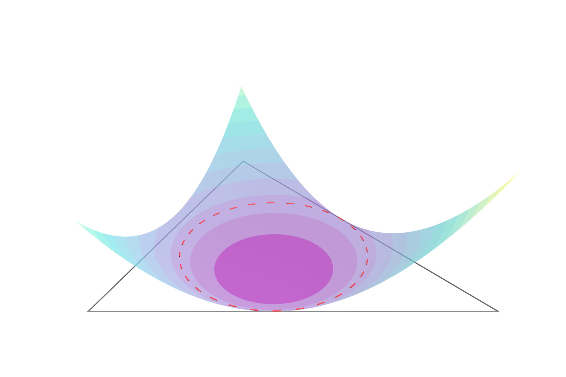
(b) Elevation plot of a bubble function (|χ|2−hT2)⋅q(|\chi|^{2}-h_{T}^{2})\cdot q on TT; the ball boundary ∂BT\partial B_{T} is highlighted in (dashed) red.
Figure 2: Sketch of element geometry and an example bubble function as in 𝕃u​(T)\mathbb{L}^{\!\!u}(T).

We define the space of vector-valued polynomials of degree at most kk on TT that vanish on ∂BT\partial B_{T} as

𝔹0k​(T):=ℙk​(T)∩H01​(BT).\mathbb{B}^{k}_{0}(T)\mathrel{\mathop{\mathchar 58\relax}}=\mathbb{P}^{k}(T)\cap H^{1}_{0}(B_{T}).

This is the first part in the definition of each velocity component of 𝕃u​(T)\mathbb{L}^{\!\!u}(T). The construction of this space allows to relate the Laplacian appearing in KT,wK_{T,w} to the H1H^{1}-semi norm — at least on BTB_{T} — through partial integration: (−Δ​uh,qh)BT=(∇uh,∇qh)BT(-\Delta u_{h},q_{h})_{B_{T}}=(\nabla u_{h},\nabla q_{h})_{B_{T}} for all uh∈[𝔹0k​(T)]du_{h}\in[\mathbb{B}^{k}_{0}(T)]^{d} (and suitable qhq_{h}). A ball as the domain for fixing zeros is chosen so that we can factor out the quadratic bubble (|χ|2−hT2)(|\chi|^{2}-h_{T}^{2}) and characterize

𝔹0k​(T)=(|χ|2−hT2)​ℙk−2​(T)⇒dim([𝔹0k​(T)]d)=d⋅dim(ℙk−2​(T)).\mathbb{B}^{k}_{0}(T)=(|\chi|^{2}-h_{T}^{2})\mathbb{P}^{k-2}(T)\quad\Rightarrow\quad\dim([\mathbb{B}^{k}_{0}(T)]^{d})=d\cdot\dim(\mathbb{P}^{k-2}(T)).

The next part in the construction of the velocity component 𝕃u​(T)\mathbb{L}^{\!\!u}(T) of 𝕃⁡(T)\mathbb{L}(T) is designed to control the net fluxes on the element and the facets. Each element in span⁡{χ}\Span\{\chi\} has constant divergence and is introduced to have an explicit degree of freedom — lying in the kernel of −ν​Δ-\nu\Delta — to control the mean flux on the element. The additional dd-dimensional space of constant vectors span⁡{nT,1,…,nT,d}(=ℝd)\Span\{n_{T,1},\ldots,n_{T,d}\}(=\mathbb{R}^{d}) is introduced to similarly control the mean flux on the first dd facets of the element while lying in the kernel of KT,wK_{T,w}.

In the final step, we make use of the added degrees of freedom in the second step to constrain the mean flux on the first dd facets to zero. We hence define:

𝕃u(T):={uh∈[𝔹0k(T)]d+span{χ,nT,1,…,nT,d}:∫FT,iuh⋅nT,i=0,i=1,…,d},\mathbb{L}^{\!\!u}(T)\mathrel{\mathop{\mathchar 58\relax}}=\{u_{h}\in[\mathbb{B}^{k}_{0}(T)]^{d}+\Span\{\chi,n_{T,1},\ldots,n_{T,d}\}\mathrel{\mathop{\mathchar 58\relax}}\int_{F_{T,i}}u_{h}\cdot n_{T,i}=0,i=1,\ldots,d\}, (𝕃u\mathbb{L}^{\!\!u})

and find dim(𝕃u​(T))=dim([𝔹0k​(T)]d)+d+1−d=dim([ℙk−2​(T)]d)+1\dim(\mathbb{L}^{\!\!u}(T))=\dim([\mathbb{B}^{k}_{0}(T)]^{d})+d+1-d=\dim([\mathbb{P}^{k-2}(T)]^{d})+1. Note that the remaining total facet flux on FT,d+1F_{T,d+1} compensates for the accumulated divergence on the element in the sense that

∫Tdiv⁡uh=∑i=1d+1∫FT,iuh⋅nT,i=∫FT,d+1uh⋅nT,d+1∀uh∈𝕃u​(T),\int_{T}\Div u_{h}=\sum_{i=1}^{d+1}\int_{F_{T,i}}u_{h}\cdot n_{T,i}=\int_{F_{T,d+1}}u_{h}\cdot n_{T,d+1}\qquad\forall u_{h}\in\mathbb{L}^{\!\!u}(T), (8)

The main motivation for the introduction of the constants span⁡{nT,1,…,nT,d}\Span\{n_{T,1},\dots,n_{T,d}\} alongside the constraints flux constraints on the edge FT,iF_{T,i}, i=1,..,di=1,..,d is the following simple observation due to (8):

Lemma 3.1.

For all uh∈𝕃uu_{h}\in\mathbb{L}^{\!\!u} with div⁡uh|𝒯h=0\Div u_{h}|_{\mathcal{T}_{h}}=0 we have ΠF0​(uh⋅n)=0\Pi_{F}^{0}(u_{h}\cdot n)=0 on all facets F∈ℱhF\in{\mathcal{F}_{h}}.

Remark 3.2.

The space 𝕃u​(T)\mathbb{L}^{\!\!u}(T) contains no nonzero constant vectors, i.e. 𝕃u​(T)∩[ℙ0​(T)]d={0}.\mathbb{L}^{\!\!u}(T)\cap[\mathbb{P}^{0}(T)]^{d}=\{0\}. Consequently, 𝕃u​(T)\mathbb{L}^{\!\!u}(T) satisfies a Poincaré estimate and in particular, it is an admissible choice for 𝕏ps​(𝒯h)\mathbb{X}_{\rm ps}({\mathcal{T}_{h}}) in (7).

3.1.2 Pressure component of complement space

The pressure of the local problem appears only in terms of its gradient. Hence, we choose zero-mean polynomials of degree at most k−1k-1 for the pressure component of 𝕃⁡(T)\mathbb{L}(T), i.e. we define:

𝕃p(T)={p∈ℙk−1(T):∫Tp=0}.\mathbb{L}^{\!\!p}(T)=\{p\in\mathbb{P}^{k-1}(T)\mathrel{\mathop{\mathchar 58\relax}}\int_{T}p=0\}. (𝕃p\mathbb{L}^{\!\!p})

3.1.3 The velocity-pressure complement space

Putting both together we define

𝕃⁡(T)=𝕃u​(T)×𝕃p​(T).\mathbb{L}(T)=\mathbb{L}^{\!\!u}(T)\times\mathbb{L}^{\!\!p}(T). (𝕃\mathbb{L})

and find dim(𝕃⁡(T))=dim(ℙk−2​(T))+1+dim(ℙk−1​(T))−1=d⋅dim(ℙk−2​(T))+dim(ℙk−1​(T))=dim(ℚ⁡(T))\dim(\mathbb{L}(T))=\dim(\mathbb{P}^{k-2}(T))+1+\dim(\mathbb{P}^{k-1}(T))-1=d\cdot\dim(\mathbb{P}^{k-2}(T))+\dim(\mathbb{P}^{k-1}(T))=\dim(\mathbb{Q}(T)), which matches the dimension of the test space for the local problem, as required for the invertibility of the local operator KT,wK_{T,w} on 𝕃⁡(T)\mathbb{L}(T). We then compose canonically, 𝕃=𝕃⁡(𝒯h)=∏T∈𝒯h𝕃⁡(T)\mathbb{L}=\mathbb{L}({\mathcal{T}_{h}})=\prod_{T\in{\mathcal{T}_{h}}}\mathbb{L}(T).

3.2 Local operator

Having defined the complement space 𝕃⁡(T)\mathbb{L}(T) in Section 3.1, we now establish that the local operator KT,w:𝕃⁡(T)→ℚ′​(T)K_{T,w}\mathrel{\mathop{\mathchar 58\relax}}\mathbb{L}(T)\to\mathbb{Q}^{\prime}(T) is boundedly invertible. This is the key structural result that justifies the local-global splitting: invertibility of KT,wK_{T,w} on 𝕃⁡(T)\mathbb{L}(T) implies the direct-sum decomposition 𝕏=𝕋w⊕𝕃\mathbb{X}=\mathbb{T}_{w}\oplus\mathbb{L} (cf. Corollary 3.8), so every discrete function in 𝕏\mathbb{X} can be uniquely split into a Trefftz component in 𝕋w\mathbb{T}_{w} and a complement component in 𝕃\mathbb{L}, and within the Trefftz DG method the latter can be solved for (locally on each element independently).

The analysis is carried out in two steps. We first treat the Stokes case w=0w=0 in Section 3.2.1. We then extend to the Oseen case Section 3.2.2 w≠0w\neq 0 by treating the convection term as a perturbation and showing that invertibility is preserved whenever resolution is sufficient.

3.2.1 Stokes case w=0w=0

We start off with the following continuity result for the local Stokes operator KT,0K_{T,0}.

Lemma 3.3 (Continuity of KT,0K_{T,0}).

For all ξ=(u,p)∈𝕏reg\xi=(u,p)\in\mathbb{X}^{\texttt{reg}} there holds

‖K0​ξ‖ℚ′2=∑T∈𝒯h‖KT,0​ξ‖ℚ​(T)′2≤βK02​∥ξ∥𝕏,∗2,\|K_{0}\xi\|_{\mathbb{Q}^{\prime}}^{2}=\sum_{T\in{\mathcal{T}_{h}}}\|K_{T,0}\xi\|_{\mathbb{Q}(T)^{\prime}}^{2}\leq\beta_{\scalebox{0.6}{$K_{0}$}}^{2}\,\,\lVert\xi\rVert_{\mathbb{X},\ast}^{2}, (9)

with βK0>0\beta_{\scalebox{0.6}{$K_{0}$}}>0 depending only on the shape-regularity of 𝒯h{\mathcal{T}_{h}} and on kk.

Proof.

The L2L^{2} representation of K0​ξK_{0}\xi in ℚ\mathbb{Q} is (hT​ν−12​Πk−2​(−ν​Δ​u+∇p),−Πk−1​div⁡u)(h_{T}\nu^{-\frac{1}{2}}\Pi^{k-2}(-\nu\Delta u+\nabla p),-\Pi^{k-1}\Div u). With the continuity of the L2L^{2} projection we then have on each element T∈𝒯hT\in{\mathcal{T}_{h}}

‖KT,0​ξ‖ℚ​(T)′2≤‖hT​ν−12​(−ν​Δ​u+∇p)‖T2+ν​‖div⁡u‖T2,\|K_{T,0}\xi\|_{\mathbb{Q}(T)^{\prime}}^{2}\leq\|h_{T}\nu^{-\frac{1}{2}}(-\nu\Delta u+\nabla p)\|_{T}^{2}+\nu\|\Div u\|_{T}^{2},

Using Cauchy-Schwarz inequality and ‖div⁡uh‖T≤‖∇uh‖T\|\Div u_{h}\|_{T}\leq\|\nabla u_{h}\|_{T} we bound

∥KT,0ξh∥ℚ​(T)′2≤C(ν∥∇u∥T2+ν∥hTΔu∥T2+ν−1∥hT∇ph∥T2).\displaystyle\|K_{T,0}\xi_{h}\|_{\mathbb{Q}(T)^{\prime}}^{2}\leq C\Big(\nu\,\|\nabla u\|_{T}^{2}+\nu\,\|h_{T}\Delta u\|_{T}^{2}+\nu^{-1}\|h_{T}\nabla p_{h}\|_{T}^{2}\Big).

Summing over T∈𝒯hT\in{\mathcal{T}_{h}} gives (9). ∎

We now wish to verify that the local Stokes operator K0K_{0} is invertible on a suitable subspace of 𝕏\mathbb{X}. As a intermediate result, we use the following estimate for functions in the bubble space [𝔹0k​(T)]d=[ℙk​(T)∩H01​(BT)]d[\mathbb{B}^{k}_{0}(T)]^{d}=[\mathbb{P}^{k}(T)\cap H^{1}_{0}(B_{T})]^{d} enriched by span⁡{χ}\Span\{\chi\}.

Lemma 3.4 (Auxiliary estimate for a bubble space).

There exists a constant C>0C>0 depending only on kk (and dd) such that for all uh∈[𝔹0k​(T)]d⊕span⁡{χ}u_{h}\in[\mathbb{B}^{k}_{0}(T)]^{d}\oplus\Span\{\chi\} and all ph∈ℙk−1​(T)p_{h}\in\mathbb{P}^{k-1}(T) there holds

‖∇uh‖T2≤C⁡(hT2ν2​‖−ν​Δ​uh+∇ph‖T2+‖div⁡uh‖T2).\|\nabla u_{h}\|_{T}^{2}\leq C\Big(\frac{h_{T}^{2}}{\nu^{2}}\|-\nu\Delta u_{h}+\nabla p_{h}\|_{T}^{2}+\|\Div u_{h}\|_{T}^{2}\Big). (10)
Proof.

We will show (10) w.r.t. to the L2​(BT)L^{2}(B_{T})-norms, which is sufficient since the norms on TT and BTB_{T} are equivalent on the finite-dimensional space [𝔹0k​(T)]d⊕span⁡{χ}[\mathbb{B}^{k}_{0}(T)]^{d}\oplus\Span\{\chi\}. In the following we will derive a splitting uh=uℓ+u0=uℓ+u⟂+udivu_{h}=u_{\ell}+u_{0}=u_{\ell}+u_{\perp}+u_{\Div} for which the obvious estimate

‖∇uh‖BT2≤C⁡(‖∇u0‖BT2+‖∇uℓ‖BT2)=C⁡(‖∇udiv‖BT2+‖∇u⟂‖BT2+‖∇uℓ‖BT2)\|\nabla u_{h}\|_{B_{T}}^{2}\leq C\big(\|\nabla u_{0}\|_{B_{T}}^{2}+\|\nabla u_{\ell}\|_{B_{T}}^{2}\big)=C\big(\|\nabla u_{\Div}\|_{B_{T}}^{2}+\|\nabla u_{\perp}\|_{B_{T}}^{2}+\|\nabla u_{\ell}\|_{B_{T}}^{2}\big)

holds. Subsequently, we will derive the splitting and a bound for each of these summands.

1. Split off the affine part. Set

uℓ:=Π0​(div⁡uh)div⁡(χ)χ=d−1Π0(divuh)χ∈span{χ},u0:=uh−uℓ∈𝔹0k,u_{\ell}\mathrel{\mathop{\mathchar 58\relax}}=\frac{\Pi^{0}(\Div u_{h})}{\Div(\chi)}\,\chi=d^{-1}\Pi^{0}(\Div u_{h})\,\chi\in\Span\{\chi\},\qquad u_{0}\mathrel{\mathop{\mathchar 58\relax}}=u_{h}-u_{\ell}\in\mathbb{B}^{k}_{0},

so that Π0​div⁡uh=Π0​div⁡uℓ\Pi^{0}\Div u_{h}=\Pi^{0}\Div u_{\ell} and Π0​div⁡u0=0\Pi^{0}\Div u_{0}=0 and with ∇χ=I\nabla\chi=I we find ‖∇uℓ‖BT≤d−12​‖div⁡uh‖BT\|\nabla u_{\ell}\|_{B_{T}}\leq d^{-\frac{1}{2}}\|\Div u_{h}\|_{B_{T}}.

2. H01H^{1}_{0}-orthogonal decomposition of u0u_{0} into udivu_{\Div} and u⟂u_{\perp}. Let

𝔹div​(T):={v∈𝔹0k​(T)∣div⁡v=0},\mathbb{B}_{\Div}(T)\mathrel{\mathop{\mathchar 58\relax}}=\{v\in\mathbb{B}^{k}_{0}(T)\mid\Div v=0\},

and let 𝔹div⟂​(T)\mathbb{B}_{\Div}^{\perp}(T) be its orthogonal complement in 𝔹0k​(T)\mathbb{B}^{k}_{0}(T) with respect to (∇⋅,∇⋅)BT(\nabla\cdot,\nabla\cdot)_{B_{T}}. Then u0=udiv+u⟂u_{0}=u_{\Div}+u_{\perp} with udiv∈𝔹div​(T)u_{\Div}\in\mathbb{B}_{\Div}(T), u⟂∈𝔹div⟂​(T)u_{\perp}\in\mathbb{B}_{\Div}^{\perp}(T), and

‖∇u0‖BT2=‖∇udiv‖BT2+‖∇u⟂‖BT2,div⁡u0=div⁡u⟂.\|\nabla u_{0}\|_{B_{T}}^{2}=\|\nabla u_{\Div}\|_{B_{T}}^{2}+\|\nabla u_{\perp}\|_{B_{T}}^{2},\qquad\Div u_{0}=\Div u_{\perp}.

Since v↦‖div⁡v‖BTv\mapsto\|\Div v\|_{B_{T}} is a norm on the finite-dimensional space 𝔹div⟂​(T)\mathbb{B}_{\Div}^{\perp}(T), there exists c⟂>0c_{\perp}>0 depending only on kk such that

‖∇u⟂‖BT\displaystyle\|\nabla u_{\perp}\|_{B_{T}} ≤c⟂​‖div⁡u⟂‖BT=c⟂​‖div⁡u0‖BT≤‖div⁡uh‖BT+‖div⁡uℓ‖BT\displaystyle\leq c_{\perp}\|\Div u_{\perp}\|_{B_{T}}=c_{\perp}\|\Div u_{0}\|_{B_{T}}\leq\|\Div u_{h}\|_{B_{T}}+\|\Div u_{\ell}\|_{B_{T}}
≤‖div⁡uh‖BT+‖∇uℓ‖BT≤(1+d−12)​‖div⁡uh‖BT.\displaystyle\leq\|\Div u_{h}\|_{B_{T}}+\|\nabla u_{\ell}\|_{B_{T}}\leq(1+d^{-\frac{1}{2}})\|\Div u_{h}\|_{B_{T}}.

3. Stokes estimate on the divergence-free part. Since udiv∈[H01​(BT)]du_{\Div}\in[H^{1}_{0}(B_{T})]^{d} and div⁡udiv=0\Div u_{\Div}=0, we have (∇ph,udiv)BT=0(\nabla p_{h},u_{\Div})_{B_{T}}=0. Moreover uℓu_{\ell} is affine, hence Δ​uh=Δ​u0\Delta u_{h}=\Delta u_{0}. Thus, integrating by parts, Cauchy–Schwarz and Poincaré on BTB_{T}

ν​‖∇udiv‖BT2\displaystyle\nu\|\nabla u_{\Div}\|_{B_{T}}^{2} =(ν∇(u0−u⟂),∇udiv)BT=(ν∇u0,∇udiv)BT=(−νΔu0,udiv)BT\displaystyle=(\nu\nabla(u_{0}-u_{\perp}),\nabla u_{\Div})_{B_{T}}=(\nu\nabla u_{0},\nabla u_{\Div})_{B_{T}}=(-\nu\Delta u_{0},u_{\Div})_{B_{T}}
=(−ν​Δ​uh+∇ph,udiv)BT≤‖−ν​Δ​uh+∇ph‖BT​‖udiv‖BT\displaystyle=(-\nu\Delta u_{h}+\nabla p_{h},u_{\Div})_{B_{T}}\leq\|-\nu\Delta u_{h}+\nabla p_{h}\|_{B_{T}}\,\|u_{\Div}\|_{B_{T}}
≤C​‖−ν​Δ​uh+∇ph‖BT​h​‖∇udiv‖BT.\displaystyle\leq C\|-\nu\Delta u_{h}+\nabla p_{h}\|_{B_{T}}\,h\,\|\nabla u_{\Div}\|_{B_{T}}.

Hence,

‖∇udiv‖BT2≤C2​h2ν2​‖−ν​Δ​uh+∇ph‖BT2.\|\nabla u_{\Div}\|_{B_{T}}^{2}\leq C^{2}\,\frac{h^{2}}{\nu^{2}}\,\|-\nu\Delta u_{h}+\nabla p_{h}\|_{B_{T}}^{2}.

∎

With the above estimate at hand, we can now show the following result for the local Stokes operator KT,0K_{T,0} on 𝕃⁡(T)\mathbb{L}(T).

Theorem 3.5 (Stable invertibility of K0K_{0} on 𝕃\mathbb{L}).

For T∈𝒯hT\in{\mathcal{T}_{h}}, the local Stokes operator KT,0:𝕃⁡(T)→ℚ​(T)′K_{T,0}\mathrel{\mathop{\mathchar 58\relax}}\mathbb{L}(T)\to\mathbb{Q}(T)^{\prime} is a bijection. Moreover, there exists αK0>0\alpha_{\scalebox{0.6}{$K_{0}$}}>0, depending only on kk and the shape-regularity of TT (in particular through the constant in Lemma 3.4), such that for all ξh∈𝕃⁡(T)\xi_{h}\in\mathbb{L}(T) there holds

∥KT,0ξh∥T≥αK0(ν∥∇uh∥T2+νhT−1∥uh∥∂T2+ν−1∥hT∇ph∥T2)12\|K_{T,0}\xi_{h}\|_{T}\geq\alpha_{\scalebox{0.6}{$K_{0}$}}\Big(\nu\|\nabla u_{h}\|_{T}^{2}+\nu h_{T}^{-1}\|u_{h}\|_{\partial T}^{2}+\nu^{-1}\|h_{T}\nabla p_{h}\|_{T}^{2}\Big)^{\frac{1}{2}}\! (11)

Hence, K0:𝕃→ℚ′K_{0}\mathrel{\mathop{\mathchar 58\relax}}\mathbb{L}\to\mathbb{Q}^{\prime} is also a bijection and ‖K0​ξh‖ℚ′≥αK0​∥ξh∥𝕏\|K_{0}\xi_{h}\|_{\mathbb{Q}^{\prime}}\geq\alpha_{\scalebox{0.6}{$K_{0}$}}\lVert\xi_{h}\rVert_{\mathbb{X}} for all ξh∈𝕃\xi_{h}\in\mathbb{L}.

Proof.

We set uh=u~h−ucu_{h}=\tilde{u}_{h}-u_{c} with u~h∈[𝔹0k​(T)]d+span⁡{χ}\tilde{u}_{h}\in[\mathbb{B}_{0}^{k}(T)]^{d}+\Span\{\chi\}, uc∈[ℙ0​(T)]d=span⁡{nT,1,…,nT,d}u_{c}\in[\mathbb{P}^{0}(T)]^{d}=\Span\{n_{T,1},\dots,n_{T,d}\}. Explicitly ucu_{c} is the unique vector such that ∫FT,iu~h⋅nT,i=|FT,i|​uc⋅nT,i\int_{F_{T,i}}\tilde{u}_{h}\cdot n_{T,i}=|F_{T,i}|u_{c}\cdot n_{T,i} for i=1,…,di=1,\ldots,d, which is well-defined by the linear independence of nT,1,…,nT,dn_{T,1},\ldots,n_{T,d}.

The bounds for the three contributions ν​‖∇uh‖T2\nu\|\nabla u_{h}\|_{T}^{2}, ν​hT−1​‖uh‖∂T2\nu h_{T}^{-1}\|u_{h}\|_{\partial T}^{2} and ν−1∥hT∇ph∥T2\nu^{-1}\|h_{T}\nabla p_{h}\|_{T}^{2} are then shown one after another.

1. Control of ν​‖∇uh‖T2\nu\|\nabla u_{h}\|_{T}^{2}. Applying (10) yields

ν​‖∇uh‖T2=ν​‖∇u~h‖T2≤C⁡(‖hT​ν−12​(−ν​Δ​uh+∇ph)‖T2+‖ν12​div⁡uh‖T2)=C​‖KT,0​ξh‖T2.\nu\|\nabla u_{h}\|_{T}^{2}=\nu\|\nabla\tilde{u}_{h}\|_{T}^{2}\leq C\Big(\|h_{T}\nu^{-\frac{1}{2}}(-\nu\Delta u_{h}+\nabla p_{h})\|_{T}^{2}+\|\nu^{\frac{1}{2}}\Div u_{h}\|_{T}^{2}\Big)=C\,\|K_{T,0}\xi_{h}\|_{T}^{2}.

2. Control of the boundary term ν​hT−1​‖uh‖∂T2\nu h_{T}^{-1}\|u_{h}\|_{\partial T}^{2}. Due to ∫FT,iu~h⋅nT,i=|FT,i|​uc⋅nT,i\int_{F_{T,i}}\tilde{u}_{h}\cdot n_{T,i}=|F_{T,i}|u_{c}\cdot n_{T,i} for i=1,…,di=1,\ldots,d, we have

‖uh‖∂T≤‖uc‖∂T+‖u~h‖∂T≤C​‖u~h‖∂T.\|u_{h}\|_{\partial T}\leq\|u_{c}\|_{\partial T}+\|\tilde{u}_{h}\|_{\partial T}\leq C\|\tilde{u}_{h}\|_{\partial T}.

It hence suffices to show the bound for u~h\tilde{u}_{h}. By the trace inequality on TT and a Poincaré estimate on [𝔹0k​(T)]d[\mathbb{B}_{0}^{k}(T)]^{d} (exploiting that it does not contain constants),

ν​h−1​‖u~h‖∂T2≤C​ν​‖∇u~h‖T2≤(10)C​‖KT,0​ξh‖T2.\displaystyle\nu h^{-1}\|\tilde{u}_{h}\|_{\partial T}^{2}\leq C\nu\|\nabla\tilde{u}_{h}\|_{T}^{2}\stackrel{{\scriptstyle\eqref{eq:ball_est}}}{{\leq}}C\|K_{T,0}\xi_{h}\|_{T}^{2}.

3. Control of pressure contribution ν−1∥hT∇ph∥T2\nu^{-1}\|h_{T}\nabla p_{h}\|_{T}^{2}. By the triangle inequality and the inverse bound hT​‖Δ​uh‖T≤C​‖∇uh‖Th_{T}\|\Delta u_{h}\|_{T}\leq C\|\nabla u_{h}\|_{T},

∥hT∇ph∥T≤∥hT(−νΔuh+∇ph)∥T+ν∥hTΔuh∥T≤∥hT(−νΔuh+∇ph)∥T+Cν∥∇uh∥T.\|h_{T}\nabla p_{h}\|_{T}\leq\|h_{T}(-\nu\Delta u_{h}+\nabla p_{h})\|_{T}+\nu\,\|h_{T}\Delta u_{h}\|_{T}\leq\|h_{T}(-\nu\Delta u_{h}+\nabla p_{h})\|_{T}+C\,\nu\|\nabla u_{h}\|_{T}.

Multiplying by ν−1\nu^{-1} and using step 1 yields

ν−1∥hT∇ph∥T2≤C∥KT,0ξh∥T2.\nu^{-1}\|h_{T}\nabla p_{h}\|_{T}^{2}\leq C\,\|K_{T,0}\xi_{h}\|_{T}^{2}.

4. Conclusion and bijectivity. Combining the above estimates, we obtain (11). In particular, KT,0​ξh=0K_{T,0}\xi_{h}=0 implies ξh=0\xi_{h}=0, so KT,0K_{T,0} is injective on 𝕃⁡(T)\mathbb{L}(T). Since 𝕃⁡(T)\mathbb{L}(T) and ℚ⁡(T)\mathbb{Q}(T) are finite-dimensional and have the same dimension (by construction), KT,0K_{T,0} is bijective. ∎

3.2.2 Oseen case w≠0w\neq 0

Let us first analyze the role of the convective field ww in the local operator KwK_{w}. To this end we consider the difference between Oseen and Stokes operators, Kw−K0∈ℒ⁡(𝕏,ℚ′)K_{w}-K_{0}\in\mathcal{L}(\mathbb{X},\mathbb{Q}^{\prime}) and denote its L2L^{2}-representative (under the identification ℚ′≅ℚ\mathbb{Q}^{\prime}\cong\mathbb{Q}) in the velocity component as the local convection operator

Awc:[ℙk]d→[ℙk−2]d,uh↦Π𝒯hk−2​(w⋅∇uh),A^{\!\texttt{c}}_{w}\mathrel{\mathop{\mathchar 58\relax}}[\mathbb{P}^{k}]^{d}\to[\mathbb{P}^{k-2}]^{d},\qquad u_{h}\mapsto\Pi_{\mathcal{T}_{h}}^{k-2}(w\cdot\nabla u_{h}), (AwcA^{\!\texttt{c}}_{w})

with AT,wc⋅=(Awc⋅)|TA^{\!\texttt{c}}_{T,w}\cdot=(A^{\!\texttt{c}}_{w}\cdot)|_{T} for all T∈𝒯hT\in{\mathcal{T}_{h}}, so that ⟨(KT,w−KT,0)​ξh,(rh,sh)⟩T=(hT​ν−12​AT,wc​uh,rh)T\langle(K_{T,w}-K_{T,0})\xi_{h},(r_{h},s_{h})\rangle_{T}=(h_{T}\nu^{-\frac{1}{2}}\,A^{\!\texttt{c}}_{T,w}u_{h},r_{h})_{T} for all (rh,sh)∈ℚ⁡(T)(r_{h},s_{h})\in\mathbb{Q}(T), where ΠTk−2\Pi_{T}^{k-2} is the L2L^{2}-orthogonal projection from [L2​(T)]d[L^{2}(T)]^{d} to [ℙk−2​(T)]d[\mathbb{P}^{k-2}(T)]^{d}.

Lemma 3.6.

The linear map AT,(⋅)c:[L4(T)]d→ℒ([H1(T)]d,[ℙk−2(T)]d),w↦AT,wcA^{\!\texttt{c}}_{T,(\cdot)}\mathrel{\mathop{\mathchar 58\relax}}[L^{4}(T)]^{d}\to\mathcal{L}([H^{1}(T)]^{d},[\mathbb{P}^{k-2}(T)]^{d}),\penalty\ w\mapsto A^{\!\texttt{c}}_{T,w} is bounded with

‖hT​ν−12​AT,wc​u‖T≤ν12​|w|h,d​‖∇u‖T,\|h_{T}\nu^{-\frac{1}{2}}\,A^{\!\texttt{c}}_{T,w}u\|_{T}\leq\nu^{\frac{1}{2}}|w|_{h,d}\|\nabla u\|_{T}, (12a)
for all uh∈[H1​(T)]du_{h}\in[H^{1}(T)]^{d}, w∈[L4​(Ω)]dw\in[L^{4}(\Omega)]^{d}, and T∈𝒯hT\in{\mathcal{T}_{h}}. With βKw2=2​βK02+2​|w|h,d2\beta_{\scalebox{0.6}{$K_{w}$}}^{2}=2\beta_{\scalebox{0.6}{$K_{0}$}}^{2}+2|w|_{h,d}^{2} it follows
‖Kw​ξ‖ℚ′≤βKw​∥ξ∥𝕏,∗,ξ∈𝕏reg.\displaystyle\|K_{w}\xi\|_{\mathbb{Q}^{\prime}}\leq\beta_{\scalebox{0.6}{$K_{w}$}}\,\lVert\xi\rVert_{\mathbb{X},\ast},\qquad\xi\in\mathbb{X}^{\texttt{reg}}. (12b)
Proof.

For any w∈[L4​(T)]dw\in[L^{4}(T)]^{d}, u∈[H1​(T)]u\in[H^{1}(T)] we have by the dual version of the L4L^{4}-embedding (39) and Hölder’s inequality

‖hT​ν−12​AT,wc​u‖T≤C4​‖ν−12​hT1−d4​w⋅∇u‖L43​(T)≤C4​ν−12​‖h1−d4​w‖L4​(T)​‖∇u‖L2​(T).\|h_{T}\nu^{-\frac{1}{2}}\,A^{\!\texttt{c}}_{T,w}u\|_{T}\leq C_{4}\|\nu^{-\frac{1}{2}}h_{T}^{1-\frac{d}{4}}w\cdot\nabla u\|_{L^{\frac{4}{3}}(T)}\leq C_{4}\nu^{-\frac{1}{2}}\|h^{1-\frac{d}{4}}w\|_{L^{4}(T)}\|\nabla u\|_{L^{2}(T)}. (13)

Using the definition of |w|h,d|w|_{h,d}, we have C4​ν−12​‖hT1−d4​w‖L4​(T)≤ν12​|w|h,dC_{4}\,\nu^{-\frac{1}{2}}\|h_{T}^{1-\frac{d}{4}}w\|_{L^{4}(T)}\leq\nu^{\frac{1}{2}}\,|w|_{h,d}, which concludes the first part of the proof. Next, observe that

‖Kw​ξ‖ℚ′≤‖K0​ξ‖ℚ′+‖h​ν−12​AT,wc​u‖𝒯h,\displaystyle\|K_{w}\xi\|_{\mathbb{Q}^{\prime}}\leq\|K_{0}\xi\|_{\mathbb{Q}^{\prime}}+\|h\nu^{-\frac{1}{2}}\,A^{\!\texttt{c}}_{T,w}u\|_{{\mathcal{T}_{h}}},

where the first term can be bounded by Lemma 3.3 and the second term by (12a). ∎

Following the analysis in [20], we can derive invertibility and stability of the local operator KT,wK_{T,w} on 𝕃⁡(T)\mathbb{L}(T) based on the invertibility of the prototype operator KT,0K_{T,0} on 𝕃⁡(T)\mathbb{L}(T) and the proximity of KT,wK_{T,w} to KT,0K_{T,0} provided that the convection field ww is sufficiently small in the |w|h,d|w|_{h,d}-norm.

Corollary 3.7 (Stable invertibility of KwK_{w} on 𝕃\mathbb{L}).

Assume that (A1) holds with the resolution assumption

|w|h,d≤cγ<αK0,|w|_{h,d}\leq c_{\gamma}<\alpha_{\scalebox{0.6}{$K_{0}$}}, (A2)

where αK0\alpha_{\scalebox{0.6}{$K_{0}$}} is the constant from Theorem 3.5. Then the restriction Kw:𝕃→ℚ′K_{w}\mathrel{\mathop{\mathchar 58\relax}}\mathbb{L}\to\mathbb{Q}^{\prime} is invertible and

‖Kw​ξh‖ℚ′≥αKw​∥ξh∥𝕏,∀ξh∈𝕃,\|K_{w}\xi_{h}\|_{\mathbb{Q}^{\prime}}\geq\alpha_{\scalebox{0.6}{$K_{w}$}}\,\lVert\xi_{h}\rVert_{\mathbb{X}},\qquad\forall\xi_{h}\in\mathbb{L}, (14)

with αKw:=αK0−cγ.\alpha_{\scalebox{0.6}{$K_{w}$}}\mathrel{\mathop{\mathchar 58\relax}}=\alpha_{\scalebox{0.6}{$K_{0}$}}-c_{\gamma}.

Proof.

Using Lemma 3.6 we get for T∈𝒯hT\in{\mathcal{T}_{h}}

‖(KT,w−KT,0)​ξh‖T=‖hT​ν−12​AT,wc​uh‖T≤ν12​|w|h,d​‖∇uh‖T∀ξh=(uh,ph)∈𝕏⁡(T),\|(K_{T,w}-K_{T,0})\xi_{h}\|_{T}=\|h_{T}\nu^{-\frac{1}{2}}\,A^{\!\texttt{c}}_{T,w}u_{h}\|_{T}\leq\nu^{\frac{1}{2}}\,|w|_{h,d}\,\|\nabla u_{h}\|_{T}\quad\forall\xi_{h}=(u_{h},p_{h})\in\mathbb{X}(T),

and hence

‖(Kw−K0)​ξh‖ℚ′≤|w|h,d​∥ξh∥𝕏∀ξh∈𝕏.\|(K_{w}-K_{0})\xi_{h}\|_{\mathbb{Q}^{\prime}}\leq|w|_{h,d}\,\lVert\xi_{h}\rVert_{\mathbb{X}}\quad\forall\xi_{h}\in\mathbb{X}.

Using Theorem 3.5 (i.e. ‖K0​ξh‖ℚ′≥αK0​∥ξh∥𝕏\|K_{0}\xi_{h}\|_{\mathbb{Q}^{\prime}}\geq\alpha_{\scalebox{0.6}{$K_{0}$}}\lVert\xi_{h}\rVert_{\mathbb{X}} for all ξh∈𝕃\xi_{h}\in\mathbb{L}) and the resolution assumption, we obtain the perturbation bound

‖(Kw−K0)​ξh‖ℚ′≤|w|h,dαK0​‖K0​ξh‖ℚ′≤γ​‖K0​ξh‖ℚ′∀ξh∈𝕃,\|(K_{w}-K_{0})\xi_{h}\|_{\mathbb{Q}^{\prime}}\leq\frac{|w|_{h,d}}{\alpha_{\scalebox{0.6}{$K_{0}$}}}\|K_{0}\xi_{h}\|_{\mathbb{Q}^{\prime}}\leq\gamma\,\|K_{0}\xi_{h}\|_{\mathbb{Q}^{\prime}}\quad\forall\xi_{h}\in\mathbb{L},

with γ:=cγαK0<1\gamma\mathrel{\mathop{\mathchar 58\relax}}=\frac{c_{\gamma}}{\alpha_{\scalebox{0.6}{$K_{0}$}}}<1 by assumption. Now, using the Neumann series argument as in [20, Lemma 3.4] we obtain the result. ∎

3.3 Space decomposition

Building on the local invertibility of KT,w|𝕃K_{T,w}|_{\mathbb{L}} established in Section 3.2 we obtain a global-local space decomposition.

Corollary 3.8.

The local operator Kw:𝕏→ℚ′K_{w}\mathrel{\mathop{\mathchar 58\relax}}\mathbb{X}\to\mathbb{Q}^{\prime} is bijective on 𝕃\mathbb{L}, i.e. for all σh∈ℚ\sigma_{h}\in\mathbb{Q} there exists a unique ξh∈𝕃\xi_{h}\in\mathbb{L} such that Kw​ξh=σhK_{w}\xi_{h}=\sigma_{h} in ℚ′\mathbb{Q}^{\prime}. This implies the space decomposition property

𝕏=𝕋w⊕𝕃,\mathbb{X}=\mathbb{T}_{w}\oplus\mathbb{L}, (15)

i.e. for all ξh∈𝕏\xi_{h}\in\mathbb{X} there exist unique ξ𝕋∈𝕋w\xi_{\mathbb{T}}\in\mathbb{T}_{w} and ξ𝕃∈𝕃\xi_{\mathbb{L}}\in\mathbb{L} such that ξh=ξ𝕋+ξ𝕃\xi_{h}=\xi_{\mathbb{T}}+\xi_{\mathbb{L}}.

Proof.

Follows from Theorem 3.5 (Stokes case w=0w=0) and Corollary 3.7 (Oseen case w∈𝕎w\in\mathbb{W}). ∎

Remark 3.9.

The complement space 𝕃\mathbb{L} is defined independently of the convection field ww. This is essential for the analysis of the nonlinear Navier–Stokes problem: the same local complement space is used for every iterate in the Picard iteration.

Remark 3.10 (The inverse Kw−1:ℚ′→𝕃K_{w}^{-1}\mathrel{\mathop{\mathchar 58\relax}}\mathbb{Q}^{\prime}\to\mathbb{L}).

The invertibility of KwK_{w} on 𝕃\mathbb{L} allows to define the (bounded) inverse operator Kw−1:ℚ′→𝕃K_{w}^{-1}\mathrel{\mathop{\mathchar 58\relax}}\mathbb{Q}^{\prime}\to\mathbb{L}. Then, the splitting ξh=ξ𝕋+ξ𝕃\xi_{h}=\xi_{\mathbb{T}}+\xi_{\mathbb{L}} can be explicitly characterized with ξ𝕃:=Kw−1​Kw​ξh∈𝕃\xi_{\mathbb{L}}\mathrel{\mathop{\mathchar 58\relax}}=K_{w}^{-1}K_{w}\xi_{h}\in\mathbb{L} and ξ𝕋:=ξh−ξ𝕃∈𝕋\xi_{\mathbb{T}}\mathrel{\mathop{\mathchar 58\relax}}=\xi_{h}-\xi_{\mathbb{L}}\in\mathbb{T}.

4 The reduced formulation

This section draws two additional structural consequences. In Section 4.1 we project the splitting (15) onto the velocity component, yielding a direct-sum decomposition [ℙk​(𝒯h)]d=𝕋wu⊕𝕃u[\mathbb{P}^{k}({\mathcal{T}_{h}})]^{d}=\mathbb{T}_{w}^{u}\oplus\mathbb{L}^{\!\!u} with a proper velocity Trefftz space 𝕋wu\mathbb{T}_{w}^{u}. In Section 4.2 we recall the reduced formulation from the DG case, setting up the reduced formulation for the Trefftz-DG formulation, which we present in Section 4.3. There, we further restrict both spaces to their discretely divergence-free parts, eliminating the saddle-point structure and producing a reduced space on which the problem is coercive — a key property exploited in the analyses of Section 5 and the Navier–Stokes case in [38].

4.1 Decomposition of the velocity space

In the following, we will see that the decomposition (15) implies a decomposition on the velocity space. We define

𝕋wu:={uh∈[ℙk]d∣there exists ​phu∈ℙk−1​such that ​(uh,phu)∈𝕋w}.\mathbb{T}_{w}^{u}\mathrel{\mathop{\mathchar 58\relax}}=\{u_{h}\in[\mathbb{P}^{k}]^{d}\mid\text{there exists }p_{h}^{u}\in\mathbb{P}^{k-1}\text{ such that }(u_{h},p_{h}^{u})\in\mathbb{T}_{w}\}. (𝕋wu\mathbb{T}_{w}^{u})

Let us introduce the L2L^{2}-projected convection-diffusion operator

Awcd:[ℙk]d→[ℙk−2]d,vh↦−ν​Δ​vh+Πk−2​(w⋅∇vh),A_{w}^{\!\texttt{cd}}\mathrel{\mathop{\mathchar 58\relax}}[\mathbb{P}^{k}]^{d}\to[\mathbb{P}^{k-2}]^{d},v_{h}\mapsto-\nu\Delta v_{h}+\Pi^{k-2}(w\cdot\nabla v_{h}), (AwcdA_{w}^{\!\texttt{cd}})

and the L2L^{2} projection into the space ℙk−1​(T)\mathbb{P}^{k-1}(T) via gradients

Π∇,T:[L2​(T)]d→ℙk−1​(T)/ℝ,v↦arg​minqh∈ℙk−1​(T)/ℝ⁡‖∇qh−v‖T,\Pi_{\nabla,T}\mathrel{\mathop{\mathchar 58\relax}}[L^{2}(T)]^{d}\to\mathbb{P}^{k-1}(T)/\mathbb{R},\qquad v\mapsto\argmin_{q_{h}\in\mathbb{P}^{k-1}(T)/\mathbb{R}}\|\nabla q_{h}-v\|_{T}, (Π∇,T\Pi_{\nabla,T})

with Π∇:[L2​(𝒯h)]d→ℙk−1/ℙ0\Pi_{\nabla}\mathrel{\mathop{\mathchar 58\relax}}[L^{2}({\mathcal{T}_{h}})]^{d}\to\mathbb{P}^{k-1}/\mathbb{P}^{0} defined accordingly s.t. (Π∇⋅)|T=Π∇,T⋅(\Pi_{\nabla}\cdot)|_{T}=\Pi_{\nabla,T}\cdot for all T∈𝒯hT\in{\mathcal{T}_{h}}. To express the dependency between pressures and velocities in the Trefftz space we define the higher-order pressure lifting

𝒫w:[H2​(𝒯h)]d→ℙk−1/ℙ0,vh↦−Π∇​Awcd​vh.\mathcal{P}_{\!w}\mathrel{\mathop{\mathchar 58\relax}}[H^{2}({\mathcal{T}_{h}})]^{d}\to\mathbb{P}^{k-1}/\mathbb{P}^{0},\quad v_{h}\mapsto-\Pi_{\nabla}A_{w}^{\!\texttt{cd}}v_{h}. (𝒫w\mathcal{P}_{\!w})

By definition of 𝕋wu\mathbb{T}_{w}^{u} we find that for u𝕋∈𝕋wuu_{\mathbb{T}}\in\mathbb{T}_{w}^{u} there holds (Awcd+∇𝒫w)​u𝕋=0(A_{w}^{\!\texttt{cd}}+\nabla\mathcal{P}_{\!w})u_{\mathbb{T}}=0 and hence Kw​(u𝕋,𝒫w​u𝕋)=0K_{w}(u_{\mathbb{T}},\mathcal{P}_{\!w}u_{\mathbb{T}})=0 (as 𝒫w​u𝕋\mathcal{P}_{\!w}u_{\mathbb{T}} exactly maps to a pressure phup_{h}^{u} as in the definition ( T w u ) ). With these preparations we can now state the splitting of the velocity space.

Lemma 4.1.

There holds

[ℙk]d=𝕋wu⊕𝕃u,[\mathbb{P}^{k}]^{d}=\mathbb{T}_{w}^{u}\oplus\mathbb{L}^{\!\!u}, (16)

i.e. to every uh∈[ℙk]du_{h}\in[\mathbb{P}^{k}]^{d} there exist unique u𝕋∈𝕋wuu_{\mathbb{T}}\in\mathbb{T}_{w}^{u} and u𝕃∈𝕃uu_{\mathbb{L}}\in\mathbb{L}^{\!\!u} such that uh=u𝕋+u𝕃u_{h}=u_{\mathbb{T}}+u_{\mathbb{L}}. Further, the following characterizations hold

𝕋wu\displaystyle\mathbb{T}_{w}^{u} ={uh∈[ℙk]d∣(uh,𝒫w​uh)∈𝕋w}\displaystyle=\{u_{h}\in[\mathbb{P}^{k}]^{d}\mid(u_{h},\mathcal{P}_{\!w}u_{h})\in\mathbb{T}_{w}\} (17a)
and the other way around:
𝕋w\displaystyle\mathbb{T}_{w} ={(uh,𝒫w​uh+ph0)​for ​uh∈𝕋wu,ph0∈ℙ0}=(id,𝒫w)​𝕋wu⊕{0}×ℙ0.\displaystyle=\{(u_{h},\mathcal{P}_{\!w}u_{h}+p_{h}^{0})\text{ for }u_{h}\in\mathbb{T}_{w}^{u},p_{h}^{0}\in\mathbb{P}^{0}\}=(\id,\mathcal{P}_{\!w})\mathbb{T}_{w}^{u}\oplus\{0\}\times\mathbb{P}^{0}. (17b)
Proof.

For ξh∈𝕏\xi_{h}\in\mathbb{X} one easily checks that the following explicit characterization of the splitting ξh=ξ𝕋+ξ𝕃\xi_{h}=\xi_{\mathbb{T}}+\xi_{\mathbb{L}} holds:

(uh,ph)⏞ξh∈𝕏=(u𝕋,Π0​ph+𝒫w​u𝕋)⏞ξ𝕋∈𝕋+(u𝕃,ph−Π0​ph−𝒫w​u𝕋)⏞ξ𝕃∈𝕃.\overbrace{(u_{h},p_{h})}^{\xi_{h}\in\mathbb{X}}=\overbrace{(u_{\mathbb{T}},\Pi^{0}p_{h}+\mathcal{P}_{\!w}u_{\mathbb{T}})}^{\xi_{\mathbb{T}}\in\mathbb{T}}+\overbrace{(u_{\mathbb{L}},p_{h}-\Pi^{0}p_{h}-\mathcal{P}_{\!w}u_{\mathbb{T}})}^{\xi_{\mathbb{L}}\in\mathbb{L}}.

We observe that the decomposition of uhu_{h} into u𝕋u_{\mathbb{T}} and u𝕃u_{\mathbb{L}} is independent of the choice of php_{h} and hence unique (as ξ𝕋\xi_{\mathbb{T}} and ξ𝕃\xi_{\mathbb{L}} are unique). The characterizations (17) follow immediately from the definition of 𝒫w\mathcal{P}_{\!w} and the above explicit characterization of the splitting which concludes the proof. ∎

↝\leadsto
Figure 3: Schematic of obtaining the reduced problem for the standard DG method.

4.2 Reduced DG formulation

For the analysis of the nonlinear Navier–Stokes problem, it will be crucial to consider the reduced problem, i.e. the problem where a discrete divergence-constraint is implemented into the definition of a subspace of 𝕏⁡(𝒯h)\mathbb{X}(\mathcal{T}_{h}), cf. [5]. For the standard DG formulation, e.g. (DG), this would be the kernel of the discrete divergence operator bh(⋅,⋅)b_{h}(\cdot,\cdot) resulting in the reduced DG formulation (for the Oseen problem) only for the velocity (on a subspace of [ℙk]d[\mathbb{P}^{k}]^{d}): Find uh¯∈{vh∈[ℙk]d∣bh​(vh,qh)=0​∀qh∈ℙk−1}\underline{u_{h}}\in\{v_{h}\in[\mathbb{P}^{k}]^{d}\mid\,b_{h}(v_{h},q_{h})=0\,\forall q_{h}\in\mathbb{P}^{k-1}\}, s.t.

ahd​(uh¯,vh¯)+ah,wc​(uh¯,vh¯)=(f,vh¯)𝒯h∀vh¯∈{vh∈[ℙk]d∣bh​(vh,qh)=0​∀qh∈ℙk−1}.a_{h}^{\!\texttt{d}}(\underline{u_{h}},\underline{v_{h}})+a_{h,w}^{\!\texttt{c}}(\underline{u_{h}},\underline{v_{h}})=(f,\underline{v_{h}})_{{\mathcal{T}_{h}}}\qquad\forall\underline{v_{h}}\in\{v_{h}\in[\mathbb{P}^{k}]^{d}\mid\,b_{h}(v_{h},q_{h})=0\,\forall q_{h}\in\mathbb{P}^{k-1}\}.

See Fig. 3 for a schematic of the algebraic structure. Similarly to the above notation, we will use an underline ⋅¯\underline{\cdot} to indicate reduced spaces in the following.

4.3 Reduced Trefftz-DG formulation

Formulating the reduced problem for the Trefftz-DG method is more subtle, as the discrete divergence constraint is part of the Trefftz problem as well as the local problems.

Reduction of the local velocity space.

We start with the local problem. The divergence constraint is simply the second component of the local operator KT,wK_{T,w}, i.e. div⁡u𝕃=0\Div u_{\mathbb{L}}=0 for u𝕃∈𝕃uu_{\mathbb{L}}\in\mathbb{L}^{\!\!u}. Hence, the reduced local velocity space is simply

𝕃¯​(T)\displaystyle\underline{\mathbb{L}}(T) :={u𝕃r∈𝕃u(T):divu𝕃r=0},\displaystyle\mathrel{\mathop{\mathchar 58\relax}}=\{u_{\mathbb{L}}^{r}\in\mathbb{L}^{\!\!u}(T)\mathrel{\mathop{\mathchar 58\relax}}\Div u_{\mathbb{L}}^{r}=0\}, 𝕃¯=𝕃¯​(𝒯h)=∏T∈𝒯h𝕃¯​(T).\displaystyle\!\!\!\!\!\!\underline{\mathbb{L}}=\underline{\mathbb{L}}({\mathcal{T}_{h}})\!=\!\!\prod_{T\in{\mathcal{T}_{h}}}\!\!\underline{\mathbb{L}}(T). (𝕃¯\underline{\mathbb{L}})
with dim(𝕃¯)=dim(𝕃u)−dim(ℙk−1)\dim(\underline{\mathbb{L}})=\dim(\mathbb{L}^{\!\!u})-\dim(\mathbb{P}^{k-1}) as div|𝒯h:𝕃u→(ℙk−1)′\Div|_{\mathcal{T}_{h}}\mathrel{\mathop{\mathchar 58\relax}}\mathbb{L}^{\!\!u}\to(\mathbb{P}^{k-1})^{\prime} is surjective (implied by Corollary 3.7). A corresponding reduced local test space acting only on velocities and which renders (pressure) gradient fields ∇ℙk−1​(T)\nabla\mathbb{P}^{k-1}(T) invisible to the local operator is given by the L2L^{2} orthogonal complement to ∇ℙk−1​(T)\nabla\mathbb{P}^{k-1}(T) in [ℙk−2]d[\mathbb{P}^{k-2}]^{d}. We define the reduced local test space as
ℚ¯​(T)\displaystyle\underline{\mathbb{Q}}(T) :=kerΠ∇,T\displaystyle\mathrel{\mathop{\mathchar 58\relax}}=\ker\Pi_{\nabla,T}\ ℚ¯=ℚ¯​(𝒯h)=∏T∈𝒯hℚ¯​(T),\displaystyle\!\!\!\!\!\!\underline{\mathbb{Q}}=\underline{\mathbb{Q}}({\mathcal{T}_{h}})\!=\!\!\prod_{T\in{\mathcal{T}_{h}}}\!\!\underline{\mathbb{Q}}(T), (ℚ¯\underline{\mathbb{Q}})

so that ⟨rh,∇qh⟩𝒯h=0\langle r_{h},\nabla q_{h}\rangle_{{\mathcal{T}_{h}}}=0 for all rh∈ℚ¯r_{h}\in\underline{\mathbb{Q}}, qh∈ℙk−1q_{h}\in\mathbb{P}^{k-1}. The norm is given by the velocity part of the ℚ\mathbb{Q}-norm, i.e. for rh∈ℚ¯r_{h}\in\underline{\mathbb{Q}} we set

‖rh‖ℚ¯:=‖rh‖𝒯h\|r_{h}\|_{\underline{\mathbb{Q}}}\mathrel{\mathop{\mathchar 58\relax}}=\|r_{h}\|_{{\mathcal{T}_{h}}}

and the dual norm ∥⋅∥ℚ¯′\|\cdot\|_{\underline{\mathbb{Q}}^{\prime}} is defined accordingly. The dimension of the reduced test space matches the reduced local velocity space, i.e. there holds dim(ℚ¯)=dim([ℙk−2]d)−dim(∇ℙk−1)=dim(𝕃¯)\dim(\underline{\mathbb{Q}})=\dim([\mathbb{P}^{k-2}]^{d})-\dim(\nabla\mathbb{P}^{k-1})=\dim(\underline{\mathbb{L}}). We define the reduced local operator K¯T,w:[H2​(T)]d→ℚ¯​(T)′\underline{K}_{T,w}\mathrel{\mathop{\mathchar 58\relax}}[H^{2}(T)]^{d}\to\underline{\mathbb{Q}}(T)^{\prime} as

⟨K¯T,w​u¯𝕃,rh⟩T:=⟨h​ν−12​(−ν​Δ​u¯𝕃+w⋅∇u¯𝕃),rh⟩T∀u¯𝕃∈[H2​(T)]d,rh∈ℚ¯​(T).\langle\underline{K}_{T,w}\underline{u}_{\mathbb{L}},r_{h}\rangle_{T}\mathrel{\mathop{\mathchar 58\relax}}=\langle h\nu^{-\frac{1}{2}}(-\nu\Delta\underline{u}_{\mathbb{L}}+w\cdot\nabla\underline{u}_{\mathbb{L}}),r_{h}\rangle_{T}\qquad\forall\underline{u}_{\mathbb{L}}\in[H^{2}(T)]^{d},r_{h}\in\underline{\mathbb{Q}}(T). (K¯T,w\underline{K}_{T,w})

Correspondingly, we define K¯w:[H2​(𝒯h)]d→ℚ¯′\underline{K}_{w}\mathrel{\mathop{\mathchar 58\relax}}[H^{2}({\mathcal{T}_{h}})]^{d}\to\underline{\mathbb{Q}}^{\prime}. Note that the difference between AwcdA_{w}^{\!\texttt{cd}} and K¯w\underline{K}_{w} is in the treatment of arising gradient fields and the scaling.

Corollary 4.2 (Continuity and stability of K¯w\underline{K}_{w} on 𝕃¯\underline{\mathbb{L}}).

Assume that (A1) holds with the resolution assumption (A2). Then K¯w:𝕃¯→ℚ¯′\underline{K}_{w}\mathrel{\mathop{\mathchar 58\relax}}\underline{\mathbb{L}}\to\underline{\mathbb{Q}}^{\prime} is invertible. With αKw\alpha_{\scalebox{0.6}{$K_{w}$}}, βKw\beta_{\scalebox{0.6}{$K_{w}$}} as in Lemmas 3.3 and 3.7, for all u¯𝕃∈𝕃¯\underline{u}_{\mathbb{L}}\in\underline{\mathbb{L}} and u¯∈[H2​(𝒯h)]d\underline{u}\in[H^{2}({\mathcal{T}_{h}})]^{d} there holds

αKw​ν12​∥u¯𝕃∥1,h≤‖K¯w​u𝕃¯‖ℚ¯′,‖K¯w​u¯‖ℚ¯′\displaystyle\alpha_{\scalebox{0.6}{$K_{w}$}}\,\nu^{\frac{1}{2}}\lVert\underline{u}_{\mathbb{L}}\rVert_{1,h}\leq\|\underline{K}_{w}\underline{u_{\mathbb{L}}}\|_{\underline{\mathbb{Q}}^{\prime}},\qquad\|\underline{K}_{w}\underline{u}\|_{\underline{\mathbb{Q}}^{\prime}} ≤βKw​ν​∥u¯∥1,h,∗.\displaystyle\leq\beta_{\scalebox{0.6}{$K_{w}$}}\,\nu\,\lVert\underline{u}\rVert_{1,h,\ast}. (18)
Proof.

By stable invertibility of KwK_{w}, cf. Corollary 3.7, there is unique ξ𝕃=(u𝕃,p𝕃)∈𝕃\xi_{\mathbb{L}}=(u_{\mathbb{L}},p_{\mathbb{L}})\in\mathbb{L} so that Kw​ξ𝕃=(K¯w​u¯𝕃,0)K_{w}\xi_{\mathbb{L}}=(\underline{K}_{w}\underline{u}_{\mathbb{L}},0). The corresponding full local solution has velocity component u𝕃=u¯𝕃u_{\mathbb{L}}=\underline{u}_{\mathbb{L}}, while the pressure component is the unique p𝕃∈𝕃pp_{\mathbb{L}}\in\mathbb{L}^{\!\!p} such that

Kw​(u𝕃,p𝕃)=(K¯w​u¯𝕃,0)in ​ℚ′.K_{w}(u_{\mathbb{L}},p_{\mathbb{L}})=(\underline{K}_{w}\underline{u}_{\mathbb{L}},0)\quad\text{in }\mathbb{Q}^{\prime}.

and hence

‖K¯w​u¯𝕃‖ℚ¯′=‖Kw​ξ𝕃‖ℚ′≥αKw​‖ξ𝕃‖𝕏≥αKw​ν12​∥u𝕃∥1,h=αKw​ν12​∥u¯𝕃∥1,h.\|\underline{K}_{w}\underline{u}_{\mathbb{L}}\|_{\underline{\mathbb{Q}}^{\prime}}=\|K_{w}\xi_{\mathbb{L}}\|_{\mathbb{Q}^{\prime}}\geq\alpha_{\scalebox{0.6}{$K_{w}$}}\|\xi_{\mathbb{L}}\|_{\mathbb{X}}\geq\alpha_{\scalebox{0.6}{$K_{w}$}}\nu^{\frac{1}{2}}\lVert u_{\mathbb{L}}\rVert_{1,h}=\alpha_{\scalebox{0.6}{$K_{w}$}}\nu^{\frac{1}{2}}\lVert\underline{u}_{\mathbb{L}}\rVert_{1,h}.

Similarly, we find

‖K¯w​u¯‖ℚ¯′≤‖Kw​(u¯,0)‖ℚ′,\|\underline{K}_{w}\underline{u}\|_{\underline{\mathbb{Q}}^{\prime}}\leq\|K_{w}(\underline{u},0)\|_{\mathbb{Q}^{\prime}},

which concludes the proof after applying the continuity estimate (12b) to ξ=(u¯,0)\xi=(\underline{u},0). ∎

Reduction of the Trefftz velocity space

We now carry out the analogous reduction for the Trefftz space. By (17b) from Section 4.1, the Trefftz space decomposes as

𝕋w=(id,𝒫w)​𝕋wu⊕{0}×ℙ0.\mathbb{T}_{w}=(\id,\mathcal{P}_{\!w})\mathbb{T}_{w}^{u}\oplus\{0\}\times\mathbb{P}^{0}.

The form kh,wk_{h,w} is coercive on the first component (id,𝒫w)​𝕋wu(\id,\mathcal{P}_{\!w})\mathbb{T}_{w}^{u} [19], while it vanishes identically on the second component {0}×ℙ0\{0\}\times\mathbb{P}^{0}, since no coupling between pressure-only test and trial functions arises. The two components interact solely through bhb_{h}, so the global problem has the standard saddle-point structure in which {0}×ℙ0\{0\}\times\mathbb{P}^{0} serves as the Lagrange multiplier space enforcing the discrete divergence constraint; cf. Fig. 4.

Lemma 4.3 (LBB stability).

Assume (A1) and (A2). There exists a constant α0>0\alpha_{0}>0, depending only on Ω\Omega, kk, and the shape-regularity of 𝒯h{\mathcal{T}_{h}}, such that

supu𝕋∈𝕋wu∖{0}bh​(u𝕋,ph0)‖u𝕋‖1,h≥α0​‖ph0‖0,h∀ph0∈ℙ0.\sup_{u_{\mathbb{T}}\in\mathbb{T}_{w}^{u}\setminus\{0\}}\frac{b_{h}(u_{\mathbb{T}},\,p_{h}^{0})}{\|u_{\mathbb{T}}\|_{1,h}}\;\geq\;\alpha_{0}\,\|p_{h}^{0}\|_{0,h}\qquad\forall\,p_{h}^{0}\in\mathbb{P}^{0}. (19)
Proof.

Following [19, Lemma 7], to ph0∈ℙ0p_{h}^{0}\in\mathbb{P}^{0} there is uhp∈[ℙ1]d∩{divuhp|𝒯h=0}u_{h}^{p}\in[\mathbb{P}^{1}]^{d}\cap\{\Div u_{h}^{p}|_{\mathcal{T}_{h}}=0\} s.t. bh​(uhp,ph0)=‖ph0‖0,h2b_{h}(u_{h}^{p},p_{h}^{0})=\|p_{h}^{0}\|_{0,h}^{2} with ‖uhp‖1,h≤C​‖ph0‖0,h\|u_{h}^{p}\|_{1,h}\leq C\|p_{h}^{0}\|_{0,h}. As uhp∈[ℙk]du_{h}^{p}\in[\mathbb{P}^{k}]^{d}, we can uniquely decompose it into uhp=u𝕋+u𝕃u_{h}^{p}=u_{\mathbb{T}}+u_{\mathbb{L}} with u𝕋∈𝕋wuu_{\mathbb{T}}\in\mathbb{T}_{w}^{u} and u𝕃∈𝕃uu_{\mathbb{L}}\in\mathbb{L}^{u}. As further div⁡u𝕋|𝒯h=0\Div u_{\mathbb{T}}|_{{\mathcal{T}_{h}}}=0 we also have div⁡u𝕃|𝒯h=0\Div u_{\mathbb{L}}|_{{\mathcal{T}_{h}}}=0 and with Lemma 3.1 we have bh​(u𝕃,ph0)=([[u𝕃⋅n]],{{ph0}})ℱh=0b_{h}(u_{\mathbb{L}},p_{h}^{0})=([\![u_{\mathbb{L}}\cdot n]\!],\{\!\!\{p_{h}^{0}\}\!\!\})_{{\mathcal{F}_{h}}}=0 and hence bh​(u𝕋,ph0)=bh​(uhp,ph0)−bh​(u𝕃,ph0)=‖ph0‖0,h2b_{h}(u_{\mathbb{T}},p_{h}^{0})=b_{h}(u_{h}^{p},p_{h}^{0})-b_{h}(u_{\mathbb{L}},p_{h}^{0})=\|p_{h}^{0}\|_{0,h}^{2}. Further, we have K¯w​u𝕋=0\underline{K}_{w}u_{\mathbb{T}}=0 and hence K¯w​u𝕃=K¯w​uhp\underline{K}_{w}u_{\mathbb{L}}=\underline{K}_{w}u_{h}^{p} which yields ‖u𝕃‖1,h≤‖K¯w−1‖​‖K¯w‖​‖uhp‖1,h\|u_{\mathbb{L}}\|_{1,h}\leq\|\underline{K}_{w}^{-1}\|\|\underline{K}_{w}\|\|u_{h}^{p}\|_{1,h} and hence

‖u𝕋‖1,h≤‖uhp‖1,h+‖u𝕃‖1,h≤(1+βKwαKw)​C​‖ph0‖0,h.\|u_{\mathbb{T}}\|_{1,h}\leq\|u_{h}^{p}\|_{1,h}+\|u_{\mathbb{L}}\|_{1,h}\leq(1+\frac{\beta_{\scalebox{0.6}{$K_{w}$}}}{\alpha_{\scalebox{0.6}{$K_{w}$}}})C\|p_{h}^{0}\|_{0,h}.\vskip-17.22217pt

∎

According to this structure, we set the notation of discretely divergence-free functions as those functions uh∈[ℙk]du_{h}\in[\mathbb{P}^{k}]^{d} that are element-wise divergence-free, i.e. div⁡uh|T=0\Div u_{h}|_{T}=0 for all T∈𝒯hT\in{\mathcal{T}_{h}}, and satisfy the discrete divergence constraint against ℙ0\mathbb{P}^{0} pressure test functions, i.e. bh​(uh,qh0)=0b_{h}(u_{h},q_{h}^{0})=0 for all qh0∈ℙ0q_{h}^{0}\in\mathbb{P}^{0}:

𝕏¯:={uh∈[ℙk]d∣bh​(uh,qh0)=0​∀qh0∈ℙ0​and ​div|𝒯h​uh=0}.\underline{\mathbb{X}}\mathrel{\mathop{\mathchar 58\relax}}=\{u_{h}\in[\mathbb{P}^{k}]^{d}\mid\,b_{h}(u_{h},q_{h}^{0})=0\penalty\ \forall q_{h}^{0}\in\mathbb{P}^{0}\text{ and }\Div|_{{\mathcal{T}_{h}}}u_{h}=0\}. (𝕏¯\underline{\mathbb{X}})

In analogy to 𝕏reg\mathbb{X}^{\texttt{reg}} we introduce the notation 𝕏¯reg:=[H2​(𝒯h)]d\underline{\mathbb{X}}^{\texttt{reg}}\mathrel{\mathop{\mathchar 58\relax}}=[H^{2}({\mathcal{T}_{h}})]^{d}. The subspace of 𝕏¯\underline{\mathbb{X}} of discretely divergence-free velocity Trefftz functions is then

𝕋¯w={u𝕋¯∈𝕋wu:bh(u𝕋¯,qh0)=0∀qh0∈ℙ0}⊂𝕋wu.\underline{\mathbb{T}}_{w}=\{\underline{u_{\mathbb{T}}}\in\mathbb{T}_{w}^{u}\mathrel{\mathop{\mathchar 58\relax}}b_{h}(\underline{u_{\mathbb{T}}},q_{h}^{0})=0\penalty\ \forall q_{h}^{0}\in\mathbb{P}^{0}\}\subset\mathbb{T}_{w}^{u}. (𝕋¯w\underline{\mathbb{T}}_{w})

We obviously have 𝕃¯⊆𝕏¯\underline{\mathbb{L}}\subseteq\underline{\mathbb{X}} and 𝕋¯w⊆𝕏¯\underline{\mathbb{T}}_{w}\subseteq\underline{\mathbb{X}}. Dimension counting shows that

dim(𝕋¯w)+dim(𝕃¯)=dim(𝕋wu)−dim(ℙ0)+dim(𝕃u)−dim(ℙk−1)\displaystyle\dim(\underline{\mathbb{T}}_{w})+\dim(\underline{\mathbb{L}})=\dim(\mathbb{T}_{w}^{u})-\dim(\mathbb{P}^{0})+\dim(\mathbb{L}^{\!\!u})-\dim(\mathbb{P}^{k-1})
=dim([ℙk]d)−dim([ℙk−2]d)−2​dim(ℙ0)+dim([ℙk−2]d)+dim(ℙ0)−dim(ℙk−1)=dim(𝕏¯),\displaystyle=\dim([\mathbb{P}^{k}]^{d})-\dim([\mathbb{P}^{k-2}]^{d})-2\dim(\mathbb{P}^{0})+\dim([\mathbb{P}^{k-2}]^{d})+\dim(\mathbb{P}^{0})-\dim(\mathbb{P}^{k-1})=\dim(\underline{\mathbb{X}}),

and hence we also have the space decomposition of the discretely divergence-free velocities into Trefftz velocities in 𝕋¯w\underline{\mathbb{T}}_{w} and complement 𝕃¯\underline{\mathbb{L}}:

𝕋¯w⊕𝕃¯=𝕏¯.\underline{\mathbb{T}}_{w}\oplus\underline{\mathbb{L}}=\underline{\mathbb{X}}. (20)
↝\leadsto
Figure 4: Algebraic structure before and after reformulation as a reduced problem on 𝕏¯\underline{\mathbb{X}}.

Next, we want to use this reduction to formulate a Trefftz-DG method on 𝕏¯\underline{\mathbb{X}} that yields an equivalent velocity solution to the formulation (3).

Find u¯h=u¯𝕋+u¯𝕃∈𝕏¯\underline{u}_{h}=\underline{u}_{\mathbb{T}}+\underline{u}_{\mathbb{L}}\in\underline{\mathbb{X}} such that for all z¯h=(v¯𝕋,r¯h)∈ℤ¯:=𝕋¯w×ℚ¯\underline{z}_{h}=(\underline{v}_{\mathbb{T}},\underline{r}_{h})\in\underline{\mathbb{Z}}\mathrel{\mathop{\mathchar 58\relax}}=\underline{\mathbb{T}}_{w}\times\underline{\mathbb{Q}} there holds

c¯h,w​(u¯h,z¯h)\displaystyle\underline{c}_{h,w}(\underline{u}_{h},\underline{z}_{h}) =ℓ¯h(v¯𝕋,r¯h),with c¯h,w(u¯h,z¯h):=k¯h,w(u¯h,v¯𝕋)+⟨K¯wu¯h,r¯h⟩𝒯h,\displaystyle=\underline{\ell}_{h}(\underline{v}_{\mathbb{T}},\underline{r}_{h}),\text{ with }\underline{c}_{h,w}(\underline{u}_{h},\underline{z}_{h})\mathrel{\mathop{\mathchar 58\relax}}=\underline{k}_{h,w}(\underline{u}_{h},\underline{v}_{\mathbb{T}})+\langle\underline{K}_{w}\underline{u}_{h},\underline{r}_{h}\rangle_{{\mathcal{T}_{h}}},\penalty\ \penalty\ (c¯h,w\underline{c}_{h,w})
where ​k¯h,w​(u¯,v¯)\displaystyle\text{ where }\underline{k}_{h,w}(\underline{u},\underline{v}) :=kh,w((u¯,𝒫wu¯),(v¯,𝒫wv¯))\displaystyle\mathrel{\mathop{\mathchar 58\relax}}=k_{h,w}((\underline{u},\mathcal{P}_{\!w}\underline{u}),(\underline{v},\mathcal{P}_{\!w}\underline{v})) (k¯h,w\underline{k}_{h,w})
and ​ℓ¯h​(v¯,r¯)\displaystyle\text{ and }\underline{\ell}_{h}(\underline{v},\underline{r}) :=(f,v¯)𝒯h−bh(v¯,Π∇f)+(f,hν−12r¯)𝒯h.\displaystyle\mathrel{\mathop{\mathchar 58\relax}}=(f,\underline{v})_{\mathcal{T}_{h}}-b_{h}(\underline{v},\Pi_{\nabla}f)+(f,h\nu^{-\frac{1}{2}}\underline{r})_{\mathcal{T}_{h}}. (ℓ¯h\underline{\ell}_{h})
Theorem 4.4 (Equivalence of (3) and ( ¯ c h , w )).

Under the assumptions of Corollary 3.7, the two formulations are equivalent: any solution (uh,ph)∈𝕏(u_{h},p_{h})\in\mathbb{X} of (3) has uh∈𝕏¯u_{h}\in\underline{\mathbb{X}} satisfying ( ¯ c h , w ), and conversely, any solution u¯h∈𝕏¯\underline{u}_{h}\in\underline{\mathbb{X}} of ( ¯ c h , w ) is the velocity component of a solution of (3).

Proof.

Let ξh=(uh,ph)∈𝕏\xi_{h}=(u_{h},p_{h})\in\mathbb{X} be solution to (3). We decompose ξh=ξ𝕋+ξ𝕃\xi_{h}=\xi_{\mathbb{T}}+\xi_{\mathbb{L}}, i.e (uh,ph)=(u𝕋,p𝕋)+(u𝕃,p𝕃)(u_{h},p_{h})=(u_{\mathbb{T}},p_{\mathbb{T}})+(u_{\mathbb{L}},p_{\mathbb{L}}) and have from the second equation of the local problem that div⁡uh|𝒯h=0\Div u_{h}|_{\mathcal{T}_{h}}=0. With the second Trefftz condition, we hence have div⁡uh|𝒯h=div⁡u𝕋|𝒯h=div⁡u𝕃|𝒯h=0\Div u_{h}|_{\mathcal{T}_{h}}=\Div u_{\mathbb{T}}|_{\mathcal{T}_{h}}=\Div u_{\mathbb{L}}|_{\mathcal{T}_{h}}=0. Further, testing (3) with (0,qh0)(0,q_{h}^{0}) for qh0∈ℙ0q_{h}^{0}\in\mathbb{P}^{0} we find – together with Lemma 3.1 – that we have bh​(uh,qh0)=bh​(u𝕋,qh0)=bh​(u𝕃,qh0)=0b_{h}(u_{h},q_{h}^{0})=b_{h}(u_{\mathbb{T}},q_{h}^{0})=b_{h}(u_{\mathbb{L}},q_{h}^{0})=0. Hence, uh,u𝕃,u𝕋∈𝕏¯u_{h},u_{\mathbb{L}},u_{\mathbb{T}}\in\underline{\mathbb{X}} and ξ𝕋=(u𝕋,𝒫w​u𝕋+ph0)\xi_{\mathbb{T}}=(u_{\mathbb{T}},\mathcal{P}_{\!w}u_{\mathbb{T}}+p_{h}^{0}), ph0∈ℙ0p_{h}^{0}\in\mathbb{P}^{0} so that u𝕋∈𝕋¯wu_{\mathbb{T}}\in\underline{\mathbb{T}}_{w} and u𝕃∈𝕃¯u_{\mathbb{L}}\in\underline{\mathbb{L}}. Writing out the first equation of the Trefftz condition we get

Awcd​uh+∇ph=Awcd​u𝕃+∇p𝕃=Πk−2​f.A_{w}^{\!\texttt{cd}}u_{h}+\nabla p_{h}=A_{w}^{\!\texttt{cd}}u_{\mathbb{L}}+\nabla p_{\mathbb{L}}=\Pi^{k-2}f.

With u𝕃∈𝕃¯u_{\mathbb{L}}\in\underline{\mathbb{L}} so that K¯w​u𝕃=h​ν−12​f\underline{K}_{w}u_{\mathbb{L}}=h\nu^{-\frac{1}{2}}f in ℚ¯′\underline{\mathbb{Q}}^{\prime} and p𝕃=Π∇​(f−Awcd​u𝕃)=Π∇​f+𝒫w​u𝕃p_{\mathbb{L}}=\Pi_{\nabla}(f-A_{w}^{\!\texttt{cd}}u_{\mathbb{L}})=\Pi_{\nabla}f+\mathcal{P}_{\!w}u_{\mathbb{L}} we found an expression for the unique solution ξ𝕃\xi_{\mathbb{L}} (uniqueness followed from Corollary 3.7). We conclude ξ𝕋=(u𝕋,𝒫w​u𝕋+ph0)\xi_{\mathbb{T}}=(u_{\mathbb{T}},\mathcal{P}_{\!w}u_{\mathbb{T}}+p_{h}^{0}) for u𝕋∈𝕋¯w,ph0∈ℙ0u_{\mathbb{T}}\in\underline{\mathbb{T}}_{w},\penalty\ p_{h}^{0}\in\mathbb{P}^{0} and ξ𝕃=(u𝕃,𝒫w​u𝕃)+(0,Π∇​f)\xi_{\mathbb{L}}=(u_{\mathbb{L}},\mathcal{P}_{\!w}u_{\mathbb{L}})+(0,\Pi_{\nabla}f) for u𝕃∈𝕃¯u_{\mathbb{L}}\in\underline{\mathbb{L}}, hence ξh=(uh,𝒫w​uh)+(0,Π∇​f+ph0)\xi_{h}=(u_{h},\mathcal{P}_{\!w}u_{h})+(0,\Pi_{\nabla}f+p_{h}^{0}).

Now, consider Trefftz test function η𝕋∈𝕋w\eta_{\mathbb{T}}\in\mathbb{T}_{w} with η𝕋=(v𝕋,𝒫w​v𝕋)\eta_{\mathbb{T}}=(v_{\mathbb{T}},\mathcal{P}_{\!w}v_{\mathbb{T}}) for v𝕋∈𝕋¯wv_{\mathbb{T}}\in\underline{\mathbb{T}}_{w} and plug these into (3): kh,w​(ξh,η𝕋)=(f,v𝕋)𝒯hk_{h,w}(\xi_{h},\eta_{\mathbb{T}})=(f,v_{\mathbb{T}})_{\mathcal{T}_{h}}. Plugging in the previously obtained characterizations for ξ𝕃\xi_{\mathbb{L}} we find

kh,w​(ξh,η𝕋)\displaystyle k_{h,w}(\xi_{h},\eta_{\mathbb{T}}) =kh,w​((uh,𝒫w​uh),(v𝕋,𝒫w​v𝕋))+kh,w​((0,Π∇​f+ph0),(v𝕋,𝒫w​v𝕋))\displaystyle=k_{h,w}((u_{h},\mathcal{P}_{\!w}u_{h}),(v_{\mathbb{T}},\mathcal{P}_{\!w}v_{\mathbb{T}}))+k_{h,w}((0,\Pi_{\nabla}f+p_{h}^{0}),(v_{\mathbb{T}},\mathcal{P}_{\!w}v_{\mathbb{T}}))
=k¯h,w​(uh,v𝕋)+bh​(v𝕋,Π∇​f)+bh​(v𝕋,ph0)=(f,v𝕋)𝒯h∀v𝕋∈𝕋¯w.\displaystyle=\underline{k}_{h,w}(u_{h},v_{\mathbb{T}})+b_{h}(v_{\mathbb{T}},\Pi_{\nabla}f)+b_{h}(v_{\mathbb{T}},p_{h}^{0})=(f,v_{\mathbb{T}})_{\mathcal{T}_{h}}\qquad\forall v_{\mathbb{T}}\in\underline{\mathbb{T}}_{w}. (21)

As v𝕋∈𝕋¯v_{\mathbb{T}}\in\underline{\mathbb{T}} we have bh​(v𝕋,ph0)=0b_{h}(v_{\mathbb{T}},p_{h}^{0})=0 and hence, the velocity solution of (3) also solves ( ¯ c h , w ). To go the other way around let u¯h=u¯𝕋+u¯𝕃∈𝕏¯\underline{u}_{h}=\underline{u}_{\mathbb{T}}+\underline{u}_{\mathbb{L}}\in\underline{\mathbb{X}} with u¯𝕋∈𝕋¯w\underline{u}_{\mathbb{T}}\in\underline{\mathbb{T}}_{w}, u¯𝕃∈𝕃¯\underline{u}_{\mathbb{L}}\in\underline{\mathbb{L}} be the solution to ( ¯ c h , w ). From the considerations above we know already that ξ𝕃=(u¯𝕃,𝒫w​u¯𝕃+Π∇​f)\xi_{\mathbb{L}}=(\underline{u}_{\mathbb{L}},\mathcal{P}_{\!w}\underline{u}_{\mathbb{L}}+\Pi_{\nabla}f) solves the local problem of (3). For ξ𝕋\xi_{\mathbb{T}} we set ξ𝕋=(u¯𝕋,𝒫w​u¯𝕋+ph0)\xi_{\mathbb{T}}=(\underline{u}_{\mathbb{T}},\mathcal{P}_{\!w}\underline{u}_{\mathbb{T}}+p_{h}^{0}), yielding ξh=(u¯h,𝒫w​u¯h+ph0+Π∇​f)\xi_{h}=(\underline{u}_{h},\mathcal{P}_{\!w}\underline{u}_{h}+p_{h}^{0}+\Pi_{\nabla}f) for an undetermined ph0∈ℙ0p_{h}^{0}\in\mathbb{P}^{0}. Plugging in yields (21), but this time bh​(v𝕋,ph0)b_{h}(v_{\mathbb{T}},p_{h}^{0}) does not vanish as we only have v𝕋∈𝕋wuv_{\mathbb{T}}\in\mathbb{T}_{w}^{u} and not v𝕋∈𝕋¯wv_{\mathbb{T}}\in\underline{\mathbb{T}}_{w}. However, due to the LBB condition Lemma 4.3 we know that there is a unique ph0∈ℙ0p_{h}^{0}\in\mathbb{P}^{0} so that (21) indeed holds. This concludes the proof. ∎

4.3.1 Norm equivalence between velocity and lifted velocity-pressure pair

Let us define the scaled velocity norm ∥⋅∥𝕏¯:=ν12∥⋅∥1,h\lVert\cdot\rVert_{\underline{\mathbb{X}}}\mathrel{\mathop{\mathchar 58\relax}}=\nu^{\frac{1}{2}}\lVert\cdot\rVert_{1,h} on [H1​(𝒯h)]d[H^{1}({\mathcal{T}_{h}})]^{d}. and ∥⋅∥𝕏¯,∗:=ν12∥⋅∥1,h,∗\lVert\cdot\rVert_{\underline{\mathbb{X}},\ast}\mathrel{\mathop{\mathchar 58\relax}}=\nu^{\frac{1}{2}}\lVert\cdot\rVert_{1,h,\ast} on 𝕏¯reg=[H2​(𝒯h)]d\underline{\mathbb{X}}^{\texttt{reg}}=[H^{2}({\mathcal{T}_{h}})]^{d}. A key auxiliary fact, used throughout, is that the pressure lifting satisfies Π𝒯h0​𝒫w​u=0\Pi^{0}_{\mathcal{T}_{h}}\mathcal{P}_{\!w}u=0 for any u∈[H2​(𝒯h)]du\in[H^{2}({\mathcal{T}_{h}})]^{d} (since 𝒫w\mathcal{P}_{\!w} maps into ℙk−1/ℙ0\mathbb{P}^{k-1}/\mathbb{P}^{0}), and by (12b) for any u¯∈𝕏¯reg\underline{u}\in\underline{\mathbb{X}}^{\texttt{reg}}

∥u¯∥𝕏¯,∗2\displaystyle\lVert\underline{u}\rVert_{\underline{\mathbb{X}},\ast}^{2} ≤∥(u¯,𝒫wu¯)∥𝕏,∗2=∥u¯∥𝕏¯,∗2+ν−1∥h∇𝒫wu¯∥𝒯h2≤∥u¯∥𝕏¯,∗2+∥ν−12hAwcdu¯∥𝒯h2\displaystyle\leq\lVert(\underline{u},\mathcal{P}_{\!w}\underline{u})\rVert_{\mathbb{X},\ast}^{2}=\lVert\underline{u}\rVert_{\underline{\mathbb{X}},\ast}^{2}+\nu^{-1}\|h\nabla\mathcal{P}_{\!w}\underline{u}\|_{\mathcal{T}_{h}}^{2}\leq\lVert\underline{u}\rVert_{\underline{\mathbb{X}},\ast}^{2}+\|\nu^{-\frac{1}{2}}hA_{w}^{\!\texttt{cd}}\underline{u}\|_{\mathcal{T}_{h}}^{2}
≤∥u¯∥𝕏¯,∗2+‖Kw​(u¯,0)‖ℚ′2≤(12b)∥u¯∥𝕏¯,∗2+βKw2​‖(u¯,0)‖𝕏,∗2≤(1+βKw2)​∥u¯∥𝕏¯,∗2.\displaystyle\leq\lVert\underline{u}\rVert_{\underline{\mathbb{X}},\ast}^{2}+\|K_{w}(\underline{u},0)\|_{\mathbb{Q}^{\prime}}^{2}\stackrel{{\scriptstyle\eqref{eq:AKw_continuity}}}{{\leq}}\lVert\underline{u}\rVert_{\underline{\mathbb{X}},\ast}^{2}+\beta_{\scalebox{0.6}{$K_{w}$}}^{2}\|(\underline{u},0)\|_{\mathbb{X},\ast}^{2}\leq(1+\beta_{\scalebox{0.6}{$K_{w}$}}^{2})\lVert\underline{u}\rVert_{\underline{\mathbb{X}},\ast}^{2}. (22a)
On the discrete space 𝕏¯\underline{\mathbb{X}} we have by norm equivalence of ∥⋅∥1,h,∗\lVert\cdot\rVert_{1,h,\ast} and ∥⋅∥1,h\lVert\cdot\rVert_{1,h} (i.e. ∥⋅∥𝕏¯,∗\lVert\cdot\rVert_{\underline{\mathbb{X}},\ast} and ∥⋅∥𝕏¯\lVert\cdot\rVert_{\underline{\mathbb{X}}})
∥u¯h∥𝕏¯≤∥(u¯h,𝒫w​u¯h)∥𝕏≤C​(1+βKw2)12​∥u¯h∥𝕏¯​for all ​u¯h∈𝕏¯.\lVert\underline{u}_{h}\rVert_{\underline{\mathbb{X}}}\leq\lVert(\underline{u}_{h},\mathcal{P}_{\!w}\underline{u}_{h})\rVert_{\mathbb{X}}\leq C(1+\beta_{\scalebox{0.6}{$K_{w}$}}^{2})^{\frac{1}{2}}\lVert\underline{u}_{h}\rVert_{\underline{\mathbb{X}}}\text{ for all }\underline{u}_{h}\in\underline{\mathbb{X}}. (22b)

5 Analysis of the Oseen Trefftz-DG method

We establish the three fundamental stability properties of the reduced bilinear form c¯h,w\underline{c}_{h,w} from ( ¯ c h , w ): continuity, coercivity of the global part k¯h,w\underline{k}_{h,w} on the Trefftz subspace 𝕋¯w\underline{\mathbb{T}}_{w}, and an inf-sup condition. The last result yields well-posedness of ( ¯ c h , w ). We equip the test space ℤ¯=𝕋¯w×ℚ¯\underline{\mathbb{Z}}=\underline{\mathbb{T}}_{w}\times\underline{\mathbb{Q}} with the norm

‖(v¯𝕋,r¯h)‖ℤ¯2:=‖v¯𝕋‖𝕏¯2+‖r¯h‖ℚ¯2.\|(\underline{v}_{\mathbb{T}},\underline{r}_{h})\|_{\underline{\mathbb{Z}}}^{2}\mathrel{\mathop{\mathchar 58\relax}}=\|\underline{v}_{\mathbb{T}}\|_{\underline{\mathbb{X}}}^{2}+\|\underline{r}_{h}\|_{\underline{\mathbb{Q}}}^{2}. (∥⋅∥ℤ¯\|\cdot\|_{\underline{\mathbb{Z}}})

5.1 Continuity

Lemma 5.1 (Continuity).

Assume (A1). There holds

kh,w​(ξ,ηh)\displaystyle k_{h,w}(\xi,\eta_{h}) ≤βkw​∥ξ∥𝕏,∗​∥ηh∥𝕏,\displaystyle\leq\beta_{\scalebox{0.6}{$k_{w}$}}\lVert\xi\rVert_{\mathbb{X},\ast}\lVert\eta_{h}\rVert_{\mathbb{X}},\hskip-11.38092pt (u,p)=ξ\displaystyle(u,p)=\xi ∈𝕏reg,\displaystyle\in\mathbb{X}^{\texttt{reg}},\hskip-11.38092pt (vh,ph)=ηh\displaystyle(v_{h},p_{h})=\eta_{h} ∈𝕏,\displaystyle\in\mathbb{X}, (23a)
ch,w​(ξ,ζh)\displaystyle c_{h,w}(\xi,\zeta_{h}) ≤βcw​∥ξ∥𝕏,∗​∥ζh∥ℤ,\displaystyle\leq\beta_{\scalebox{0.6}{$c_{w}$}}\lVert\xi\rVert_{\mathbb{X},\ast}\lVert\zeta_{h}\rVert_{\mathbb{Z}},\hskip-11.38092pt (u,p)=ξ\displaystyle(u,p)=\xi ∈𝕏reg,\displaystyle\in\mathbb{X}^{\texttt{reg}},\hskip-11.38092pt (η𝕋,σh)=ζh\displaystyle(\eta_{\mathbb{T}},\sigma_{h})=\zeta_{h} ∈ℤw,\displaystyle\in\mathbb{Z}_{w}, (23b)
k¯h,w​(u¯,v¯h)\displaystyle\underline{k}_{h,w}(\underline{u},\underline{v}_{h}) ≤βk¯w​∥u¯∥𝕏¯,∗​∥v¯h∥𝕏¯,\displaystyle\leq\beta_{\scalebox{0.6}{$\underline{k}_{w}$}}\lVert\underline{u}\rVert_{\underline{\mathbb{X}},\ast}\lVert\underline{v}_{h}\rVert_{\underline{\mathbb{X}}},\hskip-11.38092pt u¯\displaystyle\underline{u} ∈𝕏¯reg,\displaystyle\in\underline{\mathbb{X}}^{\texttt{reg}},\hskip-11.38092pt v¯h\displaystyle\underline{v}_{h} ∈𝕏¯,\displaystyle\in\underline{\mathbb{X}}, (23c)
c¯h,w​(u¯,z¯h)\displaystyle\underline{c}_{h,w}(\underline{u},\underline{z}_{h}) ≤βc¯w​∥u¯∥𝕏¯,∗​∥z¯h∥ℤ¯,\displaystyle\leq\beta_{\scalebox{0.6}{$\underline{c}_{w}$}}\lVert\underline{u}\rVert_{\underline{\mathbb{X}},\ast}\lVert\underline{z}_{h}\rVert_{\underline{\mathbb{Z}}},\hskip-11.38092pt u¯\displaystyle\underline{u} ∈𝕏¯reg,\displaystyle\in\underline{\mathbb{X}}^{\texttt{reg}},\hskip-11.38092pt (v¯𝕋,r¯h)=z¯h\displaystyle(\underline{v}_{\mathbb{T}},\underline{r}_{h})=\underline{z}_{h} ∈ℤ¯w,\displaystyle\in\underline{\mathbb{Z}}_{w}, (23d)
k¯h,w​(u¯𝕃,u¯𝕋)\displaystyle\underline{k}_{h,w}(\underline{u}_{\mathbb{L}},\underline{u}_{\mathbb{T}}) ≤β×w​‖u¯𝕃‖𝕏¯​‖u¯𝕋‖𝕏¯,\displaystyle\leq\beta_{\scalebox{0.6}{$\times_{w}$}}\,\|\underline{u}_{\mathbb{L}}\|_{\underline{\mathbb{X}}}\,\|\underline{u}_{\mathbb{T}}\|_{\underline{\mathbb{X}}},\hskip-11.38092pt u¯𝕃\displaystyle\underline{u}_{\mathbb{L}} ∈𝕃¯,\displaystyle\in\underline{\mathbb{L}},\hskip-11.38092pt u¯𝕋\displaystyle\underline{u}_{\mathbb{T}} ∈𝕋¯w.\displaystyle\in\underline{\mathbb{T}}_{w}. (23e)

where the constants βkw\beta_{\scalebox{0.6}{$k_{w}$}}, βcw\beta_{\scalebox{0.6}{$c_{w}$}}, βk¯w\beta_{\scalebox{0.6}{$\underline{k}_{w}$}}, βc¯w\beta_{\scalebox{0.6}{$\underline{c}_{w}$}}, depend on the convection field through the ratio |w|1,4,h/ν|w|_{1,4,h}/\nu. In contrast, β×w\beta_{\scalebox{0.6}{$\times_{w}$}} depends on the convection field only through the resolution quantity |w|h,d|w|_{h,d}, and not through |w|1,4,h/ν|w|_{1,4,h}/\nu.

Proof.

Bounding ahd​(u,vh)≤βad​ν​∥u∥1,h,∗​∥vh∥1,ha_{h}^{\!\texttt{d}}(u,v_{h})\leq\beta_{\scalebox{0.6}{${a}^{\texttt{d}}$}}\nu\lVert u\rVert_{1,h,\ast}\lVert v_{h}\rVert_{1,h}, ah,wc​(u,vh)≤βac​|w|1,4,h​‖u‖1,h,∗​‖vh‖1,ha_{h,w}^{\!\texttt{c}}(u,v_{h})\leq\beta_{\scalebox{0.6}{${a}^{\texttt{c}}$}}|w|_{1,4,h}\|u\|_{1,h,\ast}\|v_{h}\|_{1,h} (using (5)), and bh​(u,qh)≤βb​∥u∥1,h​∥qh∥0,hb_{h}(u,q_{h})\leq\beta_{\scalebox{0.6}{$b$}}\lVert u\rVert_{1,h}\lVert q_{h}\rVert_{0,h}, bh​(vh,q)≤βb​∥vh∥1,h​∥q∥0,hb_{h}(v_{h},q)\leq\beta_{\scalebox{0.6}{$b$}}\lVert v_{h}\rVert_{1,h}\lVert q\rVert_{0,h}, we obtain the first bound (23a) with βkw=C⁡(βad+βb+βac​|w|1,4,hν).\beta_{\scalebox{0.6}{$k_{w}$}}=C\Bigl(\beta_{\scalebox{0.6}{${a}^{\texttt{d}}$}}+\beta_{\scalebox{0.6}{$b$}}+\beta_{\scalebox{0.6}{${a}^{\texttt{c}}$}}\frac{|w|_{1,4,h}}{\nu}\Bigr). The second bound (23b) then follows from (23a) and (12b) with βcw=βkw+βKw\beta_{\scalebox{0.6}{$c_{w}$}}=\beta_{\scalebox{0.6}{$k_{w}$}}+\beta_{\scalebox{0.6}{$K_{w}$}}. For (23c) we find

k¯h,w​(u¯,v¯h)=kh,w​((u¯,𝒫w​u¯),(v¯h,𝒫w​v¯h))≤βkw​∥(u¯,𝒫w​u¯)∥𝕏,∗​∥(v¯h,𝒫w​v¯h)∥𝕏≤βk¯w​∥u¯∥𝕏¯,∗​∥v¯h∥𝕏¯\underline{k}_{h,w}(\underline{u},\underline{v}_{h})=k_{h,w}((\underline{u},\mathcal{P}_{\!w}\underline{u}),(\underline{v}_{h},\mathcal{P}_{\!w}\underline{v}_{h}))\leq\beta_{\scalebox{0.6}{$k_{w}$}}\lVert(\underline{u},\mathcal{P}_{\!w}\underline{u})\rVert_{\mathbb{X},\ast}\lVert(\underline{v}_{h},\mathcal{P}_{\!w}\underline{v}_{h})\rVert_{\mathbb{X}}\leq\beta_{\scalebox{0.6}{$\underline{k}_{w}$}}\lVert\underline{u}\rVert_{\underline{\mathbb{X}},\ast}\lVert\underline{v}_{h}\rVert_{\underline{\mathbb{X}}}

with βk¯w=C⁡(1+βKw2)​βkw\beta_{\scalebox{0.6}{$\underline{k}_{w}$}}=C(1+\beta_{\scalebox{0.6}{$K_{w}$}}^{2})\beta_{\scalebox{0.6}{$k_{w}$}}. Finally, for (23d) we gather (23c) and (18) so that βc¯w=βk¯w+βKw\beta_{\scalebox{0.6}{$\underline{c}_{w}$}}=\beta_{\scalebox{0.6}{$\underline{k}_{w}$}}+\beta_{\scalebox{0.6}{$K_{w}$}}.

Finally, since u¯𝕃∈𝕃¯⊂𝕃u\underline{u}_{\mathbb{L}}\in\underline{\mathbb{L}}\subset\mathbb{L}^{\!\!u} and 𝕃u\mathbb{L}^{\!\!u} is an admissible choice for 𝕏ps​(𝒯h)\mathbb{X}_{\rm ps}({\mathcal{T}_{h}}) by Remark 3.2, the improved convection estimate (7) yields

|ah,wc​(u¯𝕃,u¯𝕋)|≤Ct,∗​ν​|w|h,d​‖u¯𝕃‖1,h​‖u¯𝕋‖1,h=Ct,∗​|w|h,d​‖u¯𝕃‖𝕏¯​‖u¯𝕋‖𝕏¯,|a_{h,w}^{\!\texttt{c}}(\underline{u}_{\mathbb{L}},\underline{u}_{\mathbb{T}})|\leq C_{t,\ast}\,\nu\,|w|_{h,d}\,\|\underline{u}_{\mathbb{L}}\|_{1,h}\,\|\underline{u}_{\mathbb{T}}\|_{1,h}=C_{t,\ast}\,|w|_{h,d}\,\|\underline{u}_{\mathbb{L}}\|_{\underline{\mathbb{X}}}\,\|\underline{u}_{\mathbb{T}}\|_{\underline{\mathbb{X}}},

with β×w:=C⁡(βad+βb​βKw+Ct,∗​|w|h,d).\beta_{\scalebox{0.6}{$\times_{w}$}}\mathrel{\mathop{\mathchar 58\relax}}=C\bigl(\beta_{\scalebox{0.6}{${a}^{\texttt{d}}$}}+\beta_{\scalebox{0.6}{$b$}}\,\beta_{\scalebox{0.6}{$K_{w}$}}+C_{t,\ast}|w|_{h,d}\bigr). ∎

5.2 Stability of the reduced formulation

We first establish stability for the reduced velocity formulation. The stability proof reflects the space decomposition 𝕏¯=𝕋¯w⊕𝕃¯\underline{\mathbb{X}}=\underline{\mathbb{T}}_{w}\oplus\underline{\mathbb{L}}. The 𝕋¯w\underline{\mathbb{T}}_{w}-component is controlled by coercivity of the reduced Oseen form k¯h,w\underline{k}_{h,w}, whereas the 𝕃¯\underline{\mathbb{L}}-component is controlled by the local residual operator K¯w\underline{K}_{w}. The interaction between the two components is bounded by the improved cross estimate (23e).

The first result, Lemma 5.2, is therefore a coercivity statement on the reduced Trefftz kernel. The second result, Theorem 5.3, then combines this coercivity with the local stability on 𝕃¯\underline{\mathbb{L}} and yields the inf-sup condition for the reduced coupled form c¯h,w\underline{c}_{h,w} on 𝕏¯×ℤ¯\underline{\mathbb{X}}\times\underline{\mathbb{Z}}. Finally, Lemma 5.4, discusses the stability of the solution map, another crucial step in preparation for the analysis of the nonlinear problem in [38].

We begin with coercivity on 𝕋¯w\underline{\mathbb{T}}_{w}. The penalty parameter is chosen large enough to absorb the pressure-lifting contribution generated by 𝒫w\mathcal{P}_{\!w}.

Lemma 5.2 (Coercivity of k¯h,w\underline{k}_{h,w} on 𝕋¯w\underline{\mathbb{T}}_{w}).

There exist λDG>0\lambda_{\texttt{DG}}>0 and C>0C>0, depending only on shape-regularity, kk, such that for the IP parameter λ≥λDG+C​βKw2\lambda\geq\lambda_{\texttt{DG}}+C\beta_{\scalebox{0.6}{$K_{w}$}}^{2} in (2a), there holds

k¯h,w​(u¯𝕋,u¯𝕋)≥αk¯w​∥u¯𝕋∥𝕏¯2∀u¯𝕋∈𝕋¯w,with ​αk¯w=12.\underline{k}_{h,w}(\underline{u}_{\mathbb{T}},\underline{u}_{\mathbb{T}})\geq\alpha_{\scalebox{0.6}{$\underline{k}_{w}$}}\lVert\underline{u}_{\mathbb{T}}\rVert_{\underline{\mathbb{X}}}^{2}\qquad\forall\,\underline{u}_{\mathbb{T}}\in\underline{\mathbb{T}}_{w},\quad\text{with }\alpha_{\scalebox{0.6}{$\underline{k}_{w}$}}=\tfrac{1}{2}. (24)
Proof.

Let ξh:=(u¯𝕋,𝒫w​u¯𝕋)∈𝕋w\xi_{h}\mathrel{\mathop{\mathchar 58\relax}}=(\underline{u}_{\mathbb{T}},\mathcal{P}_{\!w}\underline{u}_{\mathbb{T}})\in\mathbb{T}_{w}. By 2.1, ah,wc​(u¯𝕋,u¯𝕋)≥0a_{h,w}^{\!\texttt{c}}(\underline{u}_{\mathbb{T}},\underline{u}_{\mathbb{T}})\geq 0, we have

k¯h,w​(u¯𝕋,u¯𝕋)=kh,w​(ξh,ξh)≥ahd​(u¯𝕋,u¯𝕋)+2​bh​(u¯𝕋,𝒫w​u¯𝕋).\underline{k}_{h,w}(\underline{u}_{\mathbb{T}},\underline{u}_{\mathbb{T}})=k_{h,w}(\xi_{h},\xi_{h})\geq a_{h}^{\!\texttt{d}}(\underline{u}_{\mathbb{T}},\underline{u}_{\mathbb{T}})+2b_{h}(\underline{u}_{\mathbb{T}},\mathcal{P}_{\!w}\underline{u}_{\mathbb{T}}).

The SIPG form satisfies ahd​(u¯𝕋,u¯𝕋)≥34​‖u¯𝕋‖𝕏¯2+(λ−λDG)​ν​‖h−12​[[u¯𝕋]]‖ℱh2a_{h}^{\!\texttt{d}}(\underline{u}_{\mathbb{T}},\underline{u}_{\mathbb{T}})\geq\frac{3}{4}\|\underline{u}_{\mathbb{T}}\|_{\underline{\mathbb{X}}}^{2}+(\lambda-\lambda_{\texttt{DG}})\nu\|h^{-\frac{1}{2}}[\![\underline{u}_{\mathbb{T}}]\!]\|_{{\mathcal{F}_{h}}}^{2} for λ≥λDG\lambda\geq\lambda_{\texttt{DG}}. We will use the latter contribution to bound the bh(⋅,⋅)b_{h}(\cdot,\cdot) contribution. Since div⁡u¯𝕋=0\Div\underline{u}_{\mathbb{T}}=0 on each TT,

2​bh​(u¯𝕋,𝒫w​u¯𝕋)\displaystyle 2b_{h}(\underline{u}_{\mathbb{T}},\mathcal{P}_{\!w}\underline{u}_{\mathbb{T}}) =2​([[u¯𝕋⋅n]],{{𝒫w​u¯𝕋}})ℱh≤ε−1​ν​‖h−12​[[u¯𝕋]]‖ℱh2+ε​ν−1​‖h12​{{𝒫w​u¯𝕋}}‖ℱh2,\displaystyle=2([\![\underline{u}_{\mathbb{T}}\cdot n]\!],\{\!\!\{\mathcal{P}_{\!w}\underline{u}_{\mathbb{T}}\}\!\!\})_{\mathcal{F}_{h}}\leq\varepsilon^{-1}\nu\|h^{-\frac{1}{2}}[\![\underline{u}_{\mathbb{T}}]\!]\|_{{\mathcal{F}_{h}}}^{2}+\varepsilon\nu^{-1}\|h^{\frac{1}{2}}\{\!\!\{\mathcal{P}_{\!w}\underline{u}_{\mathbb{T}}\}\!\!\}\|_{{\mathcal{F}_{h}}}^{2},

where we used Cauchy–Schwarz and Young with ε>0\varepsilon>0. With the polynomial trace inequality, discrete norm equivalences and scaling arguments and the Trefftz identity as in (22a) we obtain

ν−1∥h12{{𝒫wu¯𝕋}}∥ℱh2≤Cν−1∥𝒫wu¯𝕋∥𝒯h2≤Cν−1∥h∇𝒫wu¯𝕋∥𝒯h2≤(22a)CβKw2∥u¯𝕋∥𝕏¯2.\displaystyle\nu^{-1}\|h^{\frac{1}{2}}\{\!\!\{\mathcal{P}_{\!w}\underline{u}_{\mathbb{T}}\}\!\!\}\|_{{\mathcal{F}_{h}}}^{2}\leq C\nu^{-1}\|\mathcal{P}_{\!w}\underline{u}_{\mathbb{T}}\|_{{\mathcal{T}_{h}}}^{2}\leq C\nu^{-1}\|h\nabla\mathcal{P}_{\!w}\underline{u}_{\mathbb{T}}\|_{{\mathcal{T}_{h}}}^{2}\stackrel{{\scriptstyle\eqref{eq:plift_norm}}}{{\leq}}C\beta_{\scalebox{0.6}{$K_{w}$}}^{2}\|\underline{u}_{\mathbb{T}}\|_{\underline{\mathbb{X}}}^{2}.

With ε=(4​C​βKw2)−1\varepsilon=(4C\beta_{\scalebox{0.6}{$K_{w}$}}^{2})^{-1}, the claim then follows with λ≥λDG+4​C​βKw2\lambda\geq\lambda_{\texttt{DG}}+4C\beta_{\scalebox{0.6}{$K_{w}$}}^{2} as

k¯h,w​(u¯𝕋,u¯𝕋)≥34​‖u¯𝕋‖𝕏¯2+(λ−λDG)​ν​‖h−12​[[u¯𝕋]]‖ℱh2−14​‖u¯𝕋‖𝕏¯2−4​C​βKw2​ν​‖h−12​[[u¯𝕋]]‖ℱh2.\underline{k}_{h,w}(\underline{u}_{\mathbb{T}},\underline{u}_{\mathbb{T}})\geq\frac{3}{4}\|\underline{u}_{\mathbb{T}}\|_{\underline{\mathbb{X}}}^{2}+(\lambda-\lambda_{\texttt{DG}})\nu\|h^{-\frac{1}{2}}[\![\underline{u}_{\mathbb{T}}]\!]\|_{{\mathcal{F}_{h}}}^{2}-\frac{1}{4}\|\underline{u}_{\mathbb{T}}\|_{\underline{\mathbb{X}}}^{2}-4C\beta_{\scalebox{0.6}{$K_{w}$}}^{2}\nu\|h^{-\frac{1}{2}}[\![\underline{u}_{\mathbb{T}}]\!]\|_{{\mathcal{F}_{h}}}^{2}.\vskip-11.38092pt

∎

We now extend the preceding coercivity estimate from 𝕋¯w\underline{\mathbb{T}}_{w} to the whole space 𝕏¯\underline{\mathbb{X}}. The proof tests the Trefftz component by itself and the complement component by the Riesz representative of its local residual.

Theorem 5.3 (Inf-sup stability of c¯h,w\underline{c}_{h,w}).

Assume (A1) and (A2), and let λ\lambda be as in Lemma 5.2. For all u¯h∈𝕏¯\underline{u}_{h}\in\underline{\mathbb{X}}, there holds

supz¯h∈ℤ¯∖{0}c¯h,w​(u¯h,z¯h)‖z¯h‖ℤ¯≥αc¯w​‖u¯h‖𝕏¯,\sup_{\underline{z}_{h}\in\underline{\mathbb{Z}}\setminus\{0\}}\frac{\underline{c}_{h,w}(\underline{u}_{h},\underline{z}_{h})}{\|\underline{z}_{h}\|_{\underline{\mathbb{Z}}}}\;\geq\;\alpha_{\scalebox{0.6}{$\underline{c}_{w}$}}\|\underline{u}_{h}\|_{\underline{\mathbb{X}}}, (25)

with δ:=max{1,αKw−1,β×w2αk¯w​αKw2},αc¯w:=αk¯w2​2​δ,\delta\mathrel{\mathop{\mathchar 58\relax}}=\max\left\{1,\,\alpha_{\scalebox{0.6}{$K_{w}$}}^{-1},\,\frac{\beta_{\scalebox{0.6}{$\times_{w}$}}^{2}}{\alpha_{\scalebox{0.6}{$\underline{k}_{w}$}}\alpha_{\scalebox{0.6}{$K_{w}$}}^{2}}\right\},\ \alpha_{\scalebox{0.6}{$\underline{c}_{w}$}}\mathrel{\mathop{\mathchar 58\relax}}=\frac{\alpha_{\scalebox{0.6}{$\underline{k}_{w}$}}}{2\sqrt{2}\,\delta}, where αk¯w=12\alpha_{\scalebox{0.6}{$\underline{k}_{w}$}}=\tfrac{1}{2} is the coercivity constant from Lemma 5.2 and β×w\beta_{\scalebox{0.6}{$\times_{w}$}} is the constant from (23e). Again, αc¯w\alpha_{\scalebox{0.6}{$\underline{c}_{w}$}} depends on the convection field only through the resolution quantity |w|h,d|w|_{h,d}, and not through ‖w‖1,h/ν\|w\|_{1,h}/\nu.

Proof.

Decompose u¯h=u¯𝕋+u¯𝕃∈𝕏¯\underline{u}_{h}=\underline{u}_{\mathbb{T}}+\underline{u}_{\mathbb{L}}\in\underline{\mathbb{X}} with u¯𝕋∈𝕋¯w\underline{u}_{\mathbb{T}}\in\underline{\mathbb{T}}_{w} and u¯𝕃∈𝕃¯\underline{u}_{\mathbb{L}}\in\underline{\mathbb{L}}, and choose the test function

z¯h:=(u¯𝕋,δ​r¯h)∈ℤ¯.\underline{z}_{h}\mathrel{\mathop{\mathchar 58\relax}}=\bigl(\underline{u}_{\mathbb{T}},\delta\underline{r}_{h}\bigr)\in\underline{\mathbb{Z}}.

and where r¯h∈ℚ¯\underline{r}_{h}\in\underline{\mathbb{Q}} is the Riesz representative of K¯w​u¯𝕃∈ℚ¯′\underline{K}_{w}\underline{u}_{\mathbb{L}}\in\underline{\mathbb{Q}}^{\prime}, i.e.

⟨K¯w​u¯𝕃,r¯h⟩𝒯h=‖K¯w​u¯𝕃‖ℚ¯′2=‖r¯h‖ℚ¯2.\langle\underline{K}_{w}\underline{u}_{\mathbb{L}},\underline{r}_{h}\rangle_{\mathcal{T}_{h}}=\|\underline{K}_{w}\underline{u}_{\mathbb{L}}\|_{\underline{\mathbb{Q}}^{\prime}}^{2}=\|\underline{r}_{h}\|_{\underline{\mathbb{Q}}}^{2}.

Since u¯𝕋∈𝕋¯w\underline{u}_{\mathbb{T}}\in\underline{\mathbb{T}}_{w}, we have ⟨K¯w​u¯𝕋,r¯h⟩𝒯h=0\langle\underline{K}_{w}\underline{u}_{\mathbb{T}},\underline{r}_{h}\rangle_{\mathcal{T}_{h}}=0.

Using coercivity of k¯h,w\underline{k}_{h,w} on 𝕋¯w\underline{\mathbb{T}}_{w} (Lemma 5.2), the cross-coupling bound (23e), the stability estimate from Corollary 4.2, and Young’s inequality, we obtain

c¯h,w​(u¯h,z¯h)\displaystyle\underline{c}_{h,w}(\underline{u}_{h},\underline{z}_{h}) =k¯h,w​(u¯𝕋,u¯𝕋)+k¯h,w​(u¯𝕃,u¯𝕋)+δ​⟨K¯w​u¯𝕃,r¯h⟩𝒯h\displaystyle=\underline{k}_{h,w}(\underline{u}_{\mathbb{T}},\underline{u}_{\mathbb{T}})+\underline{k}_{h,w}(\underline{u}_{\mathbb{L}},\underline{u}_{\mathbb{T}})+\delta\langle\underline{K}_{w}\underline{u}_{\mathbb{L}},\underline{r}_{h}\rangle_{\mathcal{T}_{h}}
≥αk¯w​‖u¯𝕋‖𝕏¯2−β×w​‖u¯𝕃‖𝕏¯​‖u¯𝕋‖𝕏¯+δ​‖K¯w​u¯𝕃‖ℚ¯′2\displaystyle\geq\alpha_{\scalebox{0.6}{$\underline{k}_{w}$}}\|\underline{u}_{\mathbb{T}}\|_{\underline{\mathbb{X}}}^{2}-\beta_{\scalebox{0.6}{$\times_{w}$}}\|\underline{u}_{\mathbb{L}}\|_{\underline{\mathbb{X}}}\|\underline{u}_{\mathbb{T}}\|_{\underline{\mathbb{X}}}+\delta\|\underline{K}_{w}\underline{u}_{\mathbb{L}}\|_{\underline{\mathbb{Q}}^{\prime}}^{2}
≥αk¯w​‖u¯𝕋‖𝕏¯2−β×wαKw​‖K¯w​u¯𝕃‖ℚ¯′​‖u¯𝕋‖𝕏¯+δ​‖K¯w​u¯𝕃‖ℚ¯′2\displaystyle\geq\alpha_{\scalebox{0.6}{$\underline{k}_{w}$}}\|\underline{u}_{\mathbb{T}}\|_{\underline{\mathbb{X}}}^{2}-\frac{\beta_{\scalebox{0.6}{$\times_{w}$}}}{\alpha_{\scalebox{0.6}{$K_{w}$}}}\|\underline{K}_{w}\underline{u}_{\mathbb{L}}\|_{\underline{\mathbb{Q}}^{\prime}}\|\underline{u}_{\mathbb{T}}\|_{\underline{\mathbb{X}}}+\delta\|\underline{K}_{w}\underline{u}_{\mathbb{L}}\|_{\underline{\mathbb{Q}}^{\prime}}^{2}
≥αk¯w2​‖u¯𝕋‖𝕏¯2+(δ−β×w22​αk¯w​αKw2)​‖K¯w​u¯𝕃‖ℚ¯′2\displaystyle\geq\frac{\alpha_{\scalebox{0.6}{$\underline{k}_{w}$}}}{2}\|\underline{u}_{\mathbb{T}}\|_{\underline{\mathbb{X}}}^{2}+\left(\delta-\frac{\beta_{\scalebox{0.6}{$\times_{w}$}}^{2}}{2\alpha_{\scalebox{0.6}{$\underline{k}_{w}$}}\alpha_{\scalebox{0.6}{$K_{w}$}}^{2}}\right)\|\underline{K}_{w}\underline{u}_{\mathbb{L}}\|_{\underline{\mathbb{Q}}^{\prime}}^{2}
≥αk¯w2∥u¯𝕋∥𝕏¯2+δ2∥K¯wu¯𝕃∥ℚ¯′2.=αk¯w2​δ∥z¯h∥ℤ¯2.\displaystyle\geq\frac{\alpha_{\scalebox{0.6}{$\underline{k}_{w}$}}}{2}\|\underline{u}_{\mathbb{T}}\|_{\underline{\mathbb{X}}}^{2}+\frac{\delta}{2}\|\underline{K}_{w}\underline{u}_{\mathbb{L}}\|_{\underline{\mathbb{Q}}^{\prime}}^{2}.=\frac{\alpha_{\scalebox{0.6}{$\underline{k}_{w}$}}}{2\delta}\|\underline{z}_{h}\|_{\underline{\mathbb{Z}}}^{2}.

Moreover, since δ​αKw≥1\delta\alpha_{\scalebox{0.6}{$K_{w}$}}\geq 1, the stability estimate from Corollary 4.2 gives

‖z¯h‖ℤ¯2=‖u¯𝕋‖𝕏¯2+δ2​‖K¯w​u¯𝕃‖ℚ¯′2≥‖u¯𝕋‖𝕏¯2+‖u¯𝕃‖𝕏¯2≥12​‖u¯h‖𝕏¯2.\|\underline{z}_{h}\|_{\underline{\mathbb{Z}}}^{2}=\|\underline{u}_{\mathbb{T}}\|_{\underline{\mathbb{X}}}^{2}+\delta^{2}\|\underline{K}_{w}\underline{u}_{\mathbb{L}}\|_{\underline{\mathbb{Q}}^{\prime}}^{2}\geq\|\underline{u}_{\mathbb{T}}\|_{\underline{\mathbb{X}}}^{2}+\|\underline{u}_{\mathbb{L}}\|_{\underline{\mathbb{X}}}^{2}\geq\frac{1}{2}\|\underline{u}_{h}\|_{\underline{\mathbb{X}}}^{2}.

Taking the supremum over z¯h∈ℤ¯∖{0}\underline{z}_{h}\in\underline{\mathbb{Z}}\setminus\{0\} proves (25). ∎

Lemma 5.4 (Stability of the reduced Oseen solution map).

Let wh∈𝕎w_{h}\in\mathbb{W} and let (A1) and (A2) hold, such that the reduced Oseen problem ( ¯ c h , w ) admits a unique solution denoted by u¯h\underline{u}_{h}. Then

‖u¯h‖𝕏¯≤CFαc¯wh​ν−12​‖f‖𝒯h,\|\underline{u}_{h}\|_{\underline{\mathbb{X}}}\leq\frac{C_{F}}{\alpha_{\scalebox{0.6}{$\underline{c}_{w_{h}}$}}}\nu^{-\frac{1}{2}}\|f\|_{{\mathcal{T}_{h}}}, (26)

where CF:=((CΩ+βb​h)2+h2)1/2.C_{F}\mathrel{\mathop{\mathchar 58\relax}}=\Bigl((C_{\Omega}+\beta_{\scalebox{0.6}{$b$}}h)^{2}+h^{2}\Bigr)^{1/2}. In particular, the dependence on the convection field enters only through the reduced inf-sup constant αc¯wh\alpha_{\scalebox{0.6}{$\underline{c}_{w_{h}}$}}.

Proof.

Let z¯h=(v¯𝕋,r¯h)∈ℤ¯=𝕋¯wh×ℚ¯\underline{z}_{h}=(\underline{v}_{\mathbb{T}},\underline{r}_{h})\in\underline{\mathbb{Z}}=\underline{\mathbb{T}}_{w_{h}}\times\underline{\mathbb{Q}}. The right-hand side of ( ¯ c h , w ) is

(f,v¯𝕋)𝒯h−bh​(v¯𝕋,Π∇​f)+(f,h​ν−12​r¯h)𝒯h.(f,\underline{v}_{\mathbb{T}})_{\mathcal{T}_{h}}-b_{h}(\underline{v}_{\mathbb{T}},\Pi_{\nabla}f)+(f,h\nu^{-\frac{1}{2}}\underline{r}_{h})_{\mathcal{T}_{h}}.

We bound the three terms separately. For the first term, using discrete Poincaré inequality (36),

|(f,v¯𝕋)𝒯h|≤‖f‖𝒯h​‖v¯𝕋‖𝒯h≤CΩ​‖f‖𝒯h​‖v¯𝕋‖1,h=CΩ​ν−12​‖f‖𝒯h​‖v¯𝕋‖𝕏¯.|(f,\underline{v}_{\mathbb{T}})_{\mathcal{T}_{h}}|\leq\|f\|_{{\mathcal{T}_{h}}}\|\underline{v}_{\mathbb{T}}\|_{{\mathcal{T}_{h}}}\leq C_{\Omega}\|f\|_{{\mathcal{T}_{h}}}\|\underline{v}_{\mathbb{T}}\|_{1,h}=C_{\Omega}\nu^{-\frac{1}{2}}\|f\|_{{\mathcal{T}_{h}}}\|\underline{v}_{\mathbb{T}}\|_{\underline{\mathbb{X}}}.

For the second term, by continuity of bhb_{h} and since Π∇​f∈ℙk−1/ℙ0\Pi_{\nabla}f\in\mathbb{P}^{k-1}/\mathbb{P}^{0} has elementwise mean zero, we get

∥Π∇f∥0,h=∥h∇Π∇f∥𝒯h.\|\Pi_{\nabla}f\|_{0,h}=\|h\nabla\Pi_{\nabla}f\|_{{\mathcal{T}_{h}}}.

Moreover, ∇Π∇f\nabla\Pi_{\nabla}f is the L2L^{2}-orthogonal projection of ff onto the space of discrete gradients, hence

∥∇Π∇f∥𝒯h≤∥f∥𝒯h,and therefore∥Π∇f∥0,h≤h∥f∥𝒯h,\|\nabla\Pi_{\nabla}f\|_{{\mathcal{T}_{h}}}\leq\|f\|_{{\mathcal{T}_{h}}},\qquad\text{and therefore}\qquad\|\Pi_{\nabla}f\|_{0,h}\leq h\|f\|_{{\mathcal{T}_{h}}},

and thus

|bh​(v¯𝕋,Π∇​f)|≤βb​‖v¯𝕋‖1,h​‖Π∇​f‖0,h≤βb​h​ν−12​‖f‖𝒯h​‖v¯𝕋‖𝕏¯.|b_{h}(\underline{v}_{\mathbb{T}},\Pi_{\nabla}f)|\leq\beta_{\scalebox{0.6}{$b$}}\|\underline{v}_{\mathbb{T}}\|_{1,h}\|\Pi_{\nabla}f\|_{0,h}\leq\beta_{\scalebox{0.6}{$b$}}h\nu^{-\frac{1}{2}}\|f\|_{{\mathcal{T}_{h}}}\|\underline{v}_{\mathbb{T}}\|_{\underline{\mathbb{X}}}.

For the local term there holds

|(f,h​ν−12​r¯h)𝒯h|≤h​ν−12​‖f‖𝒯h​‖r¯h‖ℚ¯.|(f,h\nu^{-\frac{1}{2}}\underline{r}_{h})_{\mathcal{T}_{h}}|\leq h\nu^{-\frac{1}{2}}\|f\|_{{\mathcal{T}_{h}}}\|\underline{r}_{h}\|_{\underline{\mathbb{Q}}}.

Collecting the three bounds gives

|(f,v¯𝕋)𝒯h−bh​(v¯𝕋,Π∇​f)+(f,h​ν−12​r¯h)𝒯h|≤ν−12​‖f‖𝒯h​((CΩ+βb​h)​‖v¯𝕋‖𝕏¯+h​‖r¯h‖ℚ¯),\bigl|(f,\underline{v}_{\mathbb{T}})_{\mathcal{T}_{h}}-b_{h}(\underline{v}_{\mathbb{T}},\Pi_{\nabla}f)+(f,h\nu^{-\frac{1}{2}}\underline{r}_{h})_{\mathcal{T}_{h}}\bigr|\leq\nu^{-\frac{1}{2}}\|f\|_{{\mathcal{T}_{h}}}\Bigl((C_{\Omega}+\beta_{\scalebox{0.6}{$b$}}h)\|\underline{v}_{\mathbb{T}}\|_{\underline{\mathbb{X}}}+h\|\underline{r}_{h}\|_{\underline{\mathbb{Q}}}\Bigr),

thus using Cauchy–Schwarz,

|(f,v¯𝕋)𝒯h−bh​(v¯𝕋,Π∇​f)+(f,h​ν−12​r¯h)𝒯h|≤CF​ν−12​‖f‖𝒯h​‖z¯h‖ℤ¯.\bigl|(f,\underline{v}_{\mathbb{T}})_{\mathcal{T}_{h}}-b_{h}(\underline{v}_{\mathbb{T}},\Pi_{\nabla}f)+(f,h\nu^{-\frac{1}{2}}\underline{r}_{h})_{\mathcal{T}_{h}}\bigr|\leq C_{F}\nu^{-\frac{1}{2}}\|f\|_{{\mathcal{T}_{h}}}\|\underline{z}_{h}\|_{\underline{\mathbb{Z}}}.

Now apply the reduced inf-sup estimate (25) from Theorem 5.3 to the solution u¯h\underline{u}_{h} of ( ¯ c h , w ):

αc¯wh​‖u¯h‖𝕏¯≤supz¯h∈ℤ¯∖{0}c¯h,wh​(u¯h,z¯h)‖z¯h‖ℤ¯=supz¯h∈ℤ¯∖{0}(f,v¯𝕋)𝒯h−bh​(v¯𝕋,Π∇​f)+(f,h​ν−12​r¯h)𝒯h‖z¯h‖ℤ¯\alpha_{\scalebox{0.6}{$\underline{c}_{w_{h}}$}}\|\underline{u}_{h}\|_{\underline{\mathbb{X}}}\leq\sup_{\underline{z}_{h}\in\underline{\mathbb{Z}}\setminus\{0\}}\frac{\underline{c}_{h,w_{h}}(\underline{u}_{h},\underline{z}_{h})}{\|\underline{z}_{h}\|_{\underline{\mathbb{Z}}}}=\sup_{\underline{z}_{h}\in\underline{\mathbb{Z}}\setminus\{0\}}\frac{(f,\underline{v}_{\mathbb{T}})_{\mathcal{T}_{h}}-b_{h}(\underline{v}_{\mathbb{T}},\Pi_{\nabla}f)+(f,h\nu^{-\frac{1}{2}}\underline{r}_{h})_{\mathcal{T}_{h}}}{\|\underline{z}_{h}\|_{\underline{\mathbb{Z}}}}

Together with the preceding bound, this gives the claim. ∎

5.3 Stability of the full formulation

We now pass from the reduced velocity formulation to the full velocity-pressure formulation. This requires two additional ingredients. First, the pressure modes which are not represented in the reduced velocity problem are controlled by the piecewise-constant LBB estimate, from Lemma 4.3. Second, the stability of the local operator on the full local complement 𝕃\mathbb{L} established in Corollary 3.7.

The resulting argument has two levels. We first prove an inf-sup estimate for the full Oseen form on the Trefftz space 𝕋w\mathbb{T}_{w}. This step combines the reduced velocity stability with the pressure control supplied by the LBB estimate. We then obtain the stability of the full coupled Trefftz formulation on 𝕏\mathbb{X} by adding the local residual equation and using the stability and continuity of KwK_{w} on the complement. The final step is done by applying the framework of [20, §2.5]

Theorem 5.5 (Inf-sup stability of the full Oseen form on 𝕋w\mathbb{T}_{w}).

Assume (A1) and (A2), and let λ\lambda be chosen as in Lemma 5.2. Then there exists a constant αkw>0\alpha_{\scalebox{0.6}{$k_{w}$}}>0 such that

supη𝕋∈𝕋w∖{0}kh,w​(ξ𝕋,η𝕋)∥η𝕋∥𝕏≥αkw​∥ξ𝕋∥𝕏∀ξ𝕋∈𝕋w,\sup_{\eta_{\mathbb{T}}\in\mathbb{T}_{w}\setminus\{0\}}\frac{k_{h,w}(\xi_{\mathbb{T}},\eta_{\mathbb{T}})}{\lVert\eta_{\mathbb{T}}\rVert_{\mathbb{X}}}\geq\alpha_{\scalebox{0.6}{$k_{w}$}}\,\lVert\xi_{\mathbb{T}}\rVert_{\mathbb{X}}\qquad\forall\,\xi_{\mathbb{T}}\in\mathbb{T}_{w}, (27)

with the constant

αkw=C​min⁡{αk¯w,α02(1+βKw2)​βkw},\alpha_{\scalebox{0.6}{$k_{w}$}}=C\min\left\{\alpha_{\scalebox{0.6}{$\underline{k}_{w}$}},\frac{\alpha_{0}^{2}}{(1+\beta_{\scalebox{0.6}{$K_{w}$}}^{2})\beta_{\scalebox{0.6}{$k_{w}$}}}\right\}, (28)

where αk¯w\alpha_{\scalebox{0.6}{$\underline{k}_{w}$}} is the coercivity constant from Lemma 5.2, α0\alpha_{0} is the constant from Lemma 4.3, with C>0C>0 a constant that depends only on the equivalence constant in (22b).

Proof.

By (17b), every ξ𝕋∈𝕋w\xi_{\mathbb{T}}\in\mathbb{T}_{w} can be written uniquely as

ξ𝕋=(u𝕋,𝒫w​u𝕋+ph0),u𝕋∈𝕋wu,ph0∈ℙ0.\xi_{\mathbb{T}}=(u_{\mathbb{T}},\mathcal{P}_{\!w}u_{\mathbb{T}}+p_{h}^{0}),\qquad u_{\mathbb{T}}\in\mathbb{T}_{w}^{u},\quad p_{h}^{0}\in\mathbb{P}^{0}.

With this splitting, the Oseen form on 𝕋w\mathbb{T}_{w} reads

kh,w​(ξ𝕋,η𝕋)=k¯h,w​(u𝕋,v𝕋)+bh​(v𝕋,ph0)+bh​(u𝕋,qh0).k_{h,w}(\xi_{\mathbb{T}},\eta_{\mathbb{T}})=\underline{k}_{h,w}(u_{\mathbb{T}},v_{\mathbb{T}})+b_{h}(v_{\mathbb{T}},p_{h}^{0})+b_{h}(u_{\mathbb{T}},q_{h}^{0}).

Thus the full Oseen form on 𝕋w\mathbb{T}_{w} has the standard saddle-point structure with velocity block k¯h,w\underline{k}_{h,w} and coupling bh(⋅,⋅)b_{h}(\cdot,\cdot) on ℙ0\mathbb{P}^{0}.

By (22b), the DG norm ∥⋅∥𝕏\lVert\cdot\rVert_{\mathbb{X}} on 𝕋w\mathbb{T}_{w} is equivalent to the natural product norm on 𝕋wu×ℙ0\mathbb{T}_{w}^{u}\times\mathbb{P}^{0}. The continuity of the full form follows from Lemma 5.1, coercivity on the kernel is exactly Lemma 5.2, and the inf-sup condition for the piecewise-constant pressure part is Lemma 4.3. The classical Babuška–Brezzi theorem therefore yields (27). Inserting the corresponding continuity, coercivity, and inf-sup constants, and using the norm equivalence (22b), gives (28). ∎

Theorem 5.6 (Inf-sup stability of the full coupled Trefftz form on 𝕏\mathbb{X}).

Assume (A1) and (A2), and let λ\lambda be chosen as in Lemma 5.2. Then there exists a constant αcw>0\alpha_{\scalebox{0.6}{$c_{w}$}}>0 such that

supζh∈ℤw∖{0}ch,w​(ξh,ζh)‖ζh‖ℤ≥αcw​∥ξh∥𝕏∀ξh∈𝕏.\sup_{\zeta_{h}\in\mathbb{Z}_{w}\setminus\{0\}}\frac{c_{h,w}(\xi_{h},\zeta_{h})}{\|\zeta_{h}\|_{\mathbb{Z}}}\geq\alpha_{\scalebox{0.6}{$c_{w}$}}\,\lVert\xi_{h}\rVert_{\mathbb{X}}\qquad\forall\,\xi_{h}\in\mathbb{X}. (29)

Moreover, one may take

αcw:=C​αkw​(1+βKw​βkw2αKw2​αkw+βKw​αkwαKw2)−1.\alpha_{\scalebox{0.6}{$c_{w}$}}\mathrel{\mathop{\mathchar 58\relax}}=C\alpha_{\scalebox{0.6}{$k_{w}$}}\left(1+\frac{\beta_{\scalebox{0.6}{$K_{w}$}}\beta_{\scalebox{0.6}{$k_{w}$}}^{2}}{\alpha_{\scalebox{0.6}{$K_{w}$}}^{2}\alpha_{\scalebox{0.6}{$k_{w}$}}}+\beta_{\scalebox{0.6}{$K_{w}$}}\frac{\alpha_{\scalebox{0.6}{$k_{w}$}}}{\alpha_{\scalebox{0.6}{$K_{w}$}}^{2}}\right)^{-1}. (30)

where αkw\alpha_{\scalebox{0.6}{$k_{w}$}} is the constant from Theorem 5.5, and C>0C>0 depends only on the norm-equivalence constants in (22b) and norm equicalence constant in ∥η∥𝕏,∗≲∥η∥𝕏\lVert\eta\rVert_{\mathbb{X},\ast}\lesssim\lVert\eta\rVert_{\mathbb{X}} for all η∈𝕏h\eta\in\mathbb{X}_{h}.

Proof.

We apply the theory of coupled Trefftz problems from [20, §2.5] (and also [37] for explicit constants). We satisfy the assumptions of the theorem as follows by the results we have established so far: lower bound on the local operator Corollary 3.7, continuity of the local operator from Lemma 3.3, inf-sup stability of the global bilinear form Theorem 5.5, continuity of the global bilinear from Lemma 5.1. This proves (29). ∎

5.4 A priori error estimates

To prove a Céa-type error estimate and a priori error estimates, we need to assume an improved consistency bound for the convection term.

Theorem 5.7 (A priori error estimate).

Assume (A1), (A2), and 2.1. Let (u,p)(u,p) be a smooth solution to the Oseen problem with u∈[Hk+1​(𝒯h)]du\in[H^{k+1}({\mathcal{T}_{h}})]^{d} and p∈Hℓ​(𝒯h)p\in H^{\ell}({\mathcal{T}_{h}}), and let u¯h∈𝕏¯\underline{u}_{h}\in\underline{\mathbb{X}} be the solution of ( ¯ c h , w ). Then for 1≤ℓ≤k1\leq\ell\leq k,

∥u−u¯h∥𝕏¯≤(1+Capp​(w)αc¯w)infv¯h∈𝕏¯Π0​v¯h=Π0​u∥u−v¯h∥𝕏¯,∗+Cpαc¯wν−1/2hℓ∥p∥Hℓ​(𝒯h),\|u-\underline{u}_{h}\|_{\underline{\mathbb{X}}}\leq\left(1+\frac{C_{\rm app}(w)}{\alpha_{\scalebox{0.6}{$\underline{c}_{w}$}}}\right)\inf_{\begin{subarray}{c}\underline{v}_{h}\in\underline{\mathbb{X}}\\ \Pi^{0}\underline{v}_{h}=\Pi^{0}u\end{subarray}}\|u-\underline{v}_{h}\|_{\underline{\mathbb{X}},\ast}+\frac{C_{p}}{\alpha_{\scalebox{0.6}{$\underline{c}_{w}$}}}\nu^{-1/2}h^{\ell}\|p\|_{H^{\ell}({\mathcal{T}_{h}})}, (31)

with

Capp(w):=βad+(2βb+1)βKw+Ct,∗|w|h,d,Cp:=C(1+βb),C_{\rm app}(w)\mathrel{\mathop{\mathchar 58\relax}}=\beta_{\scalebox{0.6}{${a}^{\texttt{d}}$}}+(2\beta_{\scalebox{0.6}{$b$}}+1)\beta_{\scalebox{0.6}{$K_{w}$}}+C_{t,\ast}|w|_{h,d},\qquad C_{p}\mathrel{\mathop{\mathchar 58\relax}}=C(1+\beta_{\scalebox{0.6}{$b$}}),

where C>0C>0 depends only on kk, dd, and the shape-regularity. In particular for k≥2k\geq 2, with the BDM interpolant v¯h=Πk𝔹​𝔻​𝕄​u∈𝕏¯\underline{v}_{h}=\Pi^{\mathbb{B}\mathbb{D}\mathbb{M}}_{k}u\in\underline{\mathbb{X}}, we have that Π0​(Πk𝔹​𝔻​𝕄​u)=Π0​u\Pi^{0}(\Pi_{k}^{\mathbb{B}\mathbb{D}\mathbb{M}}u)=\Pi^{0}u elementwise and therefore

∥u−u¯h∥𝕏¯≲hℓ​(ν12​|u|Hℓ+1​(𝒯h)+ν−12​‖p‖Hℓ​(𝒯h)).\lVert u-\underline{u}_{h}\rVert_{\underline{\mathbb{X}}}\;\lesssim\;h^{\ell}\left(\nu^{\frac{1}{2}}|u|_{H^{\ell+1}({\mathcal{T}_{h}})}\;+\;\nu^{-\frac{1}{2}}\|p\|_{H^{\ell}({\mathcal{T}_{h}})}\right). (32)
Proof.

Let v¯h∈𝕏¯\underline{v}_{h}\in\underline{\mathbb{X}} be such that eh:=u−v¯h∈𝕏ps​(𝒯h)e_{h}\mathrel{\mathop{\mathchar 58\relax}}=u-\underline{v}_{h}\in\mathbb{X}_{\rm ps}({\mathcal{T}_{h}}). By the triangle inequality and the inf-sup bound (25) applied to u¯h−v¯h\underline{u}_{h}-\underline{v}_{h},

∥u−u¯h∥𝕏¯≤∥u−v¯h∥𝕏¯+∥v¯h−u¯h∥𝕏¯,αc¯w​∥v¯h−u¯h∥𝕏¯≤supz¯h≠0c¯h,w​(u¯h−v¯h,z¯h)‖z¯h‖ℤ¯.\lVert u-\underline{u}_{h}\rVert_{\underline{\mathbb{X}}}\leq\lVert u-\underline{v}_{h}\rVert_{\underline{\mathbb{X}}}+\lVert\underline{v}_{h}-\underline{u}_{h}\rVert_{\underline{\mathbb{X}}},\qquad\alpha_{\scalebox{0.6}{$\underline{c}_{w}$}}\lVert\underline{v}_{h}-\underline{u}_{h}\rVert_{\underline{\mathbb{X}}}\leq\sup_{\underline{z}_{h}\neq 0}\frac{\underline{c}_{h,w}(\underline{u}_{h}-\underline{v}_{h},\,\underline{z}_{h})}{\|\underline{z}_{h}\|_{\underline{\mathbb{Z}}}}.

Writing z¯h=(v¯𝕋,r¯h)∈ℤ¯\underline{z}_{h}=(\underline{v}_{\mathbb{T}},\underline{r}_{h})\in\underline{\mathbb{Z}}, we split

c¯h,w(u¯h−v¯h,z¯h)=k¯h,w​(u¯h−v¯h,v¯𝕋)⏟=:I+⟨K¯w​(u¯h−v¯h),r¯h⟩𝒯h⏟=:II.\underline{c}_{h,w}(\underline{u}_{h}-\underline{v}_{h},\underline{z}_{h})=\underbrace{\underline{k}_{h,w}(\underline{u}_{h}-\underline{v}_{h},\underline{v}_{\mathbb{T}})}_{=\mathrel{\mathop{\mathchar 58\relax}}I}+\underbrace{\langle\underline{K}_{w}(\underline{u}_{h}-\underline{v}_{h}),\underline{r}_{h}\rangle_{\mathcal{T}_{h}}}_{=\mathrel{\mathop{\mathchar 58\relax}}II}.

Bound for II. For all ph0∈ℙ0p_{h}^{0}\in\mathbb{P}^{0}, by consistency of the DG bilinear form and ( ¯ c h , w ),

kh,w​((u,p−ph0),(v¯𝕋,𝒫w​v¯𝕋))\displaystyle k_{h,w}((u,p-p_{h}^{0}),(\underline{v}_{\mathbb{T}},\mathcal{P}_{\!w}\underline{v}_{\mathbb{T}})) =(f,v¯𝕋)𝒯h=kh,w​((u¯h,𝒫w​u¯h+Π∇​f),(v¯𝕋,𝒫w​v¯𝕋))∀v¯𝕋∈𝕋¯w.\displaystyle=(f,\underline{v}_{\mathbb{T}})_{\mathcal{T}_{h}}=k_{h,w}((\underline{u}_{h},\mathcal{P}_{\!w}\underline{u}_{h}+\Pi_{\nabla}f),(\underline{v}_{\mathbb{T}},\mathcal{P}_{\!w}\underline{v}_{\mathbb{T}}))\quad\forall\underline{v}_{\mathbb{T}}\in\underline{\mathbb{T}}_{w}.

Setting p~:=p−ph0−Π∇​f\tilde{p}\mathrel{\mathop{\mathchar 58\relax}}=p-p_{h}^{0}-\Pi_{\nabla}f with ph0=Π0​pp_{h}^{0}=\Pi^{0}p (so Π0​p~=0\Pi^{0}\tilde{p}=0),

kh,w​((u−u¯h,p~−𝒫w​u¯h),(v¯𝕋,𝒫w​v¯𝕋))=0∀v¯𝕋∈𝕋¯w.k_{h,w}((u-\underline{u}_{h},\,\tilde{p}-\mathcal{P}_{\!w}\underline{u}_{h}),(\underline{v}_{\mathbb{T}},\mathcal{P}_{\!w}\underline{v}_{\mathbb{T}}))=0\quad\forall\underline{v}_{\mathbb{T}}\in\underline{\mathbb{T}}_{w}. (∗\ast)

Applying ( ∗ ‣ 5.4), we obtain

I=kh,w​((u¯h−v¯h,𝒫w​(u¯h−v¯h)),(v¯𝕋,𝒫w​v¯𝕋))=kh,w​((eh,p~−𝒫w​v¯h),(v¯𝕋,𝒫w​v¯𝕋)).I=k_{h,w}((\underline{u}_{h}-\underline{v}_{h},\mathcal{P}_{\!w}(\underline{u}_{h}-\underline{v}_{h})),(\underline{v}_{\mathbb{T}},\mathcal{P}_{\!w}\underline{v}_{\mathbb{T}}))=k_{h,w}((e_{h},\tilde{p}-\mathcal{P}_{\!w}\underline{v}_{h}),(\underline{v}_{\mathbb{T}},\mathcal{P}_{\!w}\underline{v}_{\mathbb{T}})).

Using the decomposition of kh,wk_{h,w}, continuity of ahda_{h}^{\!\texttt{d}}, 2.1, continuity of bhb_{h}, and

ν−12​‖𝒫w​v¯𝕋‖0,h≤βKw​‖v¯𝕋‖𝕏¯,\nu^{-\frac{1}{2}}\|\mathcal{P}_{\!w}\underline{v}_{\mathbb{T}}\|_{0,h}\leq\beta_{\scalebox{0.6}{$K_{w}$}}\,\|\underline{v}_{\mathbb{T}}\|_{\underline{\mathbb{X}}},

we infer

|I|\displaystyle|I| ≤|ahd​(eh,v¯𝕋)|+|ah,wc​(eh,v¯𝕋)|+|bh​(eh,𝒫w​v¯𝕋)|+|bh​(v¯𝕋,p~−𝒫w​v¯h)|\displaystyle\leq|a_{h}^{\!\texttt{d}}(e_{h},\underline{v}_{\mathbb{T}})|+|a_{h,w}^{\!\texttt{c}}(e_{h},\underline{v}_{\mathbb{T}})|+|b_{h}(e_{h},\mathcal{P}_{\!w}\underline{v}_{\mathbb{T}})|+|b_{h}(\underline{v}_{\mathbb{T}},\tilde{p}-\mathcal{P}_{\!w}\underline{v}_{h})|
≤(βad+Ct,∗​|w|h,d+βb​βKw)​‖eh‖𝕏¯,∗​‖v¯𝕋‖𝕏¯+|bh​(v¯𝕋,p~−𝒫w​v¯h)|.\displaystyle\leq\Bigl(\beta_{\scalebox{0.6}{${a}^{\texttt{d}}$}}+C_{t,\ast}|w|_{h,d}+\beta_{\scalebox{0.6}{$b$}}\,\beta_{\scalebox{0.6}{$K_{w}$}}\Bigr)\|e_{h}\|_{\underline{\mathbb{X}},\ast}\,\|\underline{v}_{\mathbb{T}}\|_{\underline{\mathbb{X}}}+|b_{h}(\underline{v}_{\mathbb{T}},\tilde{p}-\mathcal{P}_{\!w}\underline{v}_{h})|.

We bound the pressure term

ν−12∥p~−𝒫wv¯h∥0,h=ν−12∥h∇(p~−𝒫wv¯h)∥𝒯h,\nu^{-\frac{1}{2}}\|\tilde{p}-\mathcal{P}_{\!w}\underline{v}_{h}\|_{0,h}=\nu^{-\frac{1}{2}}\|h\nabla(\tilde{p}-\mathcal{P}_{\!w}\underline{v}_{h})\|_{{\mathcal{T}_{h}}},

by splitting at 𝒫w​u\mathcal{P}_{\!w}u:

ν−12∥p~−𝒫wv¯h∥0,h≤ν−12∥h∇(p−Π∇f−𝒫wu)∥𝒯h⏟=:Ia+ν−12∥h∇𝒫w(u−v¯h)∥𝒯h⏟=:Ib.\nu^{-\frac{1}{2}}\|\tilde{p}-\mathcal{P}_{\!w}\underline{v}_{h}\|_{0,h}\leq\underbrace{\nu^{-\frac{1}{2}}\|h\nabla(p-\Pi_{\nabla}f-\mathcal{P}_{\!w}u)\|_{\mathcal{T}_{h}}}_{=\mathrel{\mathop{\mathchar 58\relax}}I_{a}}+\underbrace{\nu^{-\frac{1}{2}}\|h\nabla\mathcal{P}_{\!w}(u-\underline{v}_{h})\|_{\mathcal{T}_{h}}}_{=\mathrel{\mathop{\mathchar 58\relax}}I_{b}}.

For IbI_{b}: since 𝒫w=−Π∇​Awcd\mathcal{P}_{\!w}=-\Pi_{\nabla}A_{w}^{\!\texttt{cd}} (see ( P w )),

Ib=ν−12​‖h​Π∇​Awcd​(u−v¯h)‖𝒯h≤βKw​∥u−v¯h∥𝕏¯,∗.I_{b}=\nu^{-\frac{1}{2}}\|h\Pi_{\nabla}A_{w}^{\!\texttt{cd}}(u-\underline{v}_{h})\|_{\mathcal{T}_{h}}\leq\beta_{\scalebox{0.6}{$K_{w}$}}\lVert u-\underline{v}_{h}\rVert_{\underline{\mathbb{X}},\ast}.

For IaI_{a}: using Awcd​u=Πk−2​(f−∇p)A_{w}^{\!\texttt{cd}}u=\Pi^{k-2}(f-\nabla p), ( P w ), and Π∇∘Πk−2=Π∇\Pi_{\nabla}\circ\Pi^{k-2}=\Pi_{\nabla}, we find

Π∇​f+𝒫w​u=Π∇​f−Π∇​Awcd​u=Π∇​f−Π∇​(f−∇p)=Π∇​(∇p).\Pi_{\nabla}f+\mathcal{P}_{\!w}u=\Pi_{\nabla}f-\Pi_{\nabla}A_{w}^{\!\texttt{cd}}u=\Pi_{\nabla}f-\Pi_{\nabla}(f-\nabla p)=\Pi_{\nabla}(\nabla p).

Hence

∇(p−Π∇​f−𝒫w​u)=∇p−Π∇​(∇p),\nabla(p-\Pi_{\nabla}f-\mathcal{P}_{\!w}u)=\nabla p-\Pi_{\nabla}(\nabla p),

which gives

Ia≲ν−12∥h(∇p−Π∇∇p)∥𝒯h≲ν−12hℓ∥p∥Hℓ​(𝒯h),I_{a}\lesssim\nu^{-\frac{1}{2}}\|h(\nabla p-\Pi_{\nabla}\nabla p)\|_{\mathcal{T}_{h}}\lesssim\nu^{-\frac{1}{2}}h^{\ell}\|p\|_{H^{\ell}({\mathcal{T}_{h}})},

for 1≤ℓ≤k1\leq\ell\leq k by a standard Bramble–Hilbert argument. Therefore,

|bh​(v¯𝕋,p~−𝒫w​v¯h)|\displaystyle|b_{h}(\underline{v}_{\mathbb{T}},\tilde{p}-\mathcal{P}_{\!w}\underline{v}_{h})| ≤βb​‖v¯𝕋‖𝕏¯​ν−12​‖p~−𝒫w​v¯h‖0,h\displaystyle\leq\beta_{\scalebox{0.6}{$b$}}\|\underline{v}_{\mathbb{T}}\|_{\underline{\mathbb{X}}}\,\nu^{-\frac{1}{2}}\|\tilde{p}-\mathcal{P}_{\!w}\underline{v}_{h}\|_{0,h}
≤βb​(βKw​‖eh‖𝕏¯,∗+C​ν−12​hℓ​‖p‖Hℓ​(𝒯h))​‖v¯𝕋‖𝕏¯,\displaystyle\leq\beta_{\scalebox{0.6}{$b$}}\Big(\beta_{\scalebox{0.6}{$K_{w}$}}\|e_{h}\|_{\underline{\mathbb{X}},\ast}+C\,\nu^{-\frac{1}{2}}h^{\ell}\|p\|_{H^{\ell}({\mathcal{T}_{h}})}\Big)\|\underline{v}_{\mathbb{T}}\|_{\underline{\mathbb{X}}},

and hence,

|I|≤([βad+2​βb​βKw+Ct,∗​|w|h,d]​‖eh‖𝕏¯,∗+C​βb​ν−12​hℓ​‖p‖Hℓ​(𝒯h))​‖z¯h‖ℤ¯.|I|\leq\Big(\bigl[\beta_{\scalebox{0.6}{${a}^{\texttt{d}}$}}+2\beta_{\scalebox{0.6}{$b$}}\,\beta_{\scalebox{0.6}{$K_{w}$}}+C_{t,\ast}|w|_{h,d}\bigr]\|e_{h}\|_{\underline{\mathbb{X}},\ast}+C\,\beta_{\scalebox{0.6}{$b$}}\,\nu^{-\frac{1}{2}}h^{\ell}\|p\|_{H^{\ell}({\mathcal{T}_{h}})}\Big)\|\underline{z}_{h}\|_{\underline{\mathbb{Z}}}. (33)

Bound for I​III. The local equation (3b) and the PDE itself yield for r¯h∈ℚ¯\underline{r}_{h}\in\underline{\mathbb{Q}}:

⟨K¯wu,rh⟩𝒯h=⟨hν−12(−νΔu+w⋅∇u),rh⟩𝒯h=⟨−hν−12∇p,rh⟩𝒯h+⟨hν−12f,rh⟩𝒯h\displaystyle\langle\underline{K}_{w}u,r_{h}\rangle_{\mathcal{T}_{h}}=\langle h\nu^{-\frac{1}{2}}(-\nu\Delta u+w\cdot\nabla u),r_{h}\rangle_{\mathcal{T}_{h}}=\langle-h\nu^{-\frac{1}{2}}\nabla p,r_{h}\rangle_{\mathcal{T}_{h}}+\langle h\nu^{-\frac{1}{2}}f,r_{h}\rangle_{\mathcal{T}_{h}}
⟹(3b)\displaystyle\stackrel{{\scriptstyle\eqref{eq:tdgoseen:2}}}{{\Longrightarrow}}\ ⟨K¯w(u−u¯h),rh⟩𝒯h=⟨−hν−12∇p,rh⟩𝒯h=⟨hν−12∇(qh−p),rh⟩𝒯h,\displaystyle\langle\underline{K}_{w}(u-\underline{u}_{h}),r_{h}\rangle_{\mathcal{T}_{h}}=\langle-h\nu^{-\frac{1}{2}}\nabla p,r_{h}\rangle_{\mathcal{T}_{h}}=\langle h\nu^{-\frac{1}{2}}\nabla(q_{h}-p),r_{h}\rangle_{\mathcal{T}_{h}},

for any qh∈ℙk−1q_{h}\in\mathbb{P}^{k-1} where in the last step we exploited that ℚ¯\underline{\mathbb{Q}} is orthogonal to discrete gradients (r¯h⟂∇ℙk−1​(T)\underline{r}_{h}\perp\nabla\mathbb{P}^{k-1}(T)). Applying that result and continuity from (18) to I​III, we obtain:

I​I\displaystyle II =⟨K¯w(u¯h−v¯h),r¯h⟩𝒯h=⟨K¯w(u−v¯h),r¯h⟩𝒯h+⟨hν−12∇(qh−p),rh⟩𝒯h\displaystyle=\langle\underline{K}_{w}(\underline{u}_{h}-\underline{v}_{h}),\underline{r}_{h}\rangle_{\mathcal{T}_{h}}=\langle\underline{K}_{w}(u-\underline{v}_{h}),\underline{r}_{h}\rangle_{\mathcal{T}_{h}}+\langle h\nu^{-\frac{1}{2}}\nabla(q_{h}-p),r_{h}\rangle_{\mathcal{T}_{h}}
≤‖K¯w​(u−v¯h)‖ℚ¯′​‖r¯h‖ℚ¯+ν−12​infqh∈ℙk−1∥h𝒯​(p−qh)∥H1​(𝒯h)​‖r¯h‖ℚ¯\displaystyle\leq\|\underline{K}_{w}(u-\underline{v}_{h})\|_{\underline{\mathbb{Q}}^{\prime}}\,\|\underline{r}_{h}\|_{\underline{\mathbb{Q}}}+\nu^{-\frac{1}{2}}\inf_{q_{h}\in\mathbb{P}^{k-1}}\lVert h_{\mathcal{T}}(p-q_{h})\rVert_{H^{1}({\mathcal{T}_{h}})}\,\|\underline{r}_{h}\|_{\underline{\mathbb{Q}}}
≤βKw​∥u−v¯h∥𝕏¯,∗​‖z¯h‖ℤ¯+C​ν−12​hℓ​‖p‖Hℓ​(𝒯h)​‖z¯h‖ℤ¯.\displaystyle\leq\beta_{\scalebox{0.6}{$K_{w}$}}\lVert u-\underline{v}_{h}\rVert_{\underline{\mathbb{X}},\ast}\,\|\underline{z}_{h}\|_{\underline{\mathbb{Z}}}+C\nu^{-\frac{1}{2}}h^{\ell}\|p\|_{H^{\ell}({\mathcal{T}_{h}})}\,\|\underline{z}_{h}\|_{\underline{\mathbb{Z}}}.

Assembly. Combining (33) with the estimate for I​III, dividing by ‖z¯h‖ℤ¯\|\underline{z}_{h}\|_{\underline{\mathbb{Z}}}, yields

αc¯w​∥v¯h−u¯h∥𝕏¯≤Capp​(w)​∥u−v¯h∥𝕏¯,∗+Cp​ν−12​hℓ​‖p‖Hℓ​(𝒯h).\alpha_{\scalebox{0.6}{$\underline{c}_{w}$}}\lVert\underline{v}_{h}-\underline{u}_{h}\rVert_{\underline{\mathbb{X}}}\leq C_{\rm app}(w)\lVert u-\underline{v}_{h}\rVert_{\underline{\mathbb{X}},\ast}+C_{p}\,\nu^{-\frac{1}{2}}h^{\ell}\|p\|_{H^{\ell}({\mathcal{T}_{h}})}.

The triangle inequality gives

∥u−u¯h∥𝕏¯≤(1+Capp​(w)αc¯w)​∥u−v¯h∥𝕏¯,∗+Cpαc¯w​ν−12​hℓ​‖p‖Hℓ​(𝒯h).\lVert u-\underline{u}_{h}\rVert_{\underline{\mathbb{X}}}\leq\left(1+\frac{C_{\rm app}(w)}{\alpha_{\scalebox{0.6}{$\underline{c}_{w}$}}}\right)\lVert u-\underline{v}_{h}\rVert_{\underline{\mathbb{X}},\ast}+\frac{C_{p}}{\alpha_{\scalebox{0.6}{$\underline{c}_{w}$}}}\,\nu^{-\frac{1}{2}}h^{\ell}\|p\|_{H^{\ell}({\mathcal{T}_{h}})}.

Taking the infimum over all v¯h∈𝕏¯\underline{v}_{h}\in\underline{\mathbb{X}} with u−v¯h∈𝕏ps​(𝒯h)u-\underline{v}_{h}\in\mathbb{X}_{\rm ps}({\mathcal{T}_{h}}) proves (31).

For (32), the standard BDM estimate gives Πk𝔹​𝔻​𝕄​u∈[ℙk]d\Pi^{\mathbb{B}\mathbb{D}\mathbb{M}}_{k}u\in[\mathbb{P}^{k}]^{d} with Π0​(Πk𝔹​𝔻​𝕄​u)=Π0​u\Pi^{0}(\Pi_{k}^{\mathbb{B}\mathbb{D}\mathbb{M}}u)=\Pi^{0}u elementwise for k≥2k\geq 2, div⁡Πk𝔹​𝔻​𝕄​u|𝒯h=0\Div\Pi^{\mathbb{B}\mathbb{D}\mathbb{M}}_{k}u|_{\mathcal{T}_{h}}=0 (for div⁡u=0\Div u=0) and [[Πk𝔹​𝔻​𝕄​u⋅n]]=0[\![\Pi^{\mathbb{B}\mathbb{D}\mathbb{M}}_{k}u\cdot n]\!]=0 on all F∈ℱhF\in{\mathcal{F}_{h}}. Further, ∥u−Πk𝔹​𝔻​𝕄​u∥𝕏¯,∗=ν12​∥u−Πk𝔹​𝔻​𝕄​u∥1,h,∗≲ν12​hk​|u|Hk+1​(𝒯h).\lVert u-\Pi^{\mathbb{B}\mathbb{D}\mathbb{M}}_{k}u\rVert_{\underline{\mathbb{X}},\ast}=\nu^{\frac{1}{2}}\lVert u-\Pi^{\mathbb{B}\mathbb{D}\mathbb{M}}_{k}u\rVert_{1,h,\ast}\lesssim\nu^{\frac{1}{2}}h^{k}|u|_{H^{k+1}({\mathcal{T}_{h}})}. Inserting this choice into (31) yields (32). ∎

Lemma 5.8 (Pressure error bound).

Assume (A1) and (A2), and in addition w∈[Wℓ2,∞​(𝒯h)]dw\in[W^{\ell_{2},\infty}({\mathcal{T}_{h}})]^{d} for 1≤ℓ2≤k1\leq\ell_{2}\leq k. Let (u,p)(u,p) be a Oseen solution with p∈Hℓ​(𝒯h)p\in H^{\ell}({\mathcal{T}_{h}}) and let (uh,ph)∈𝕏(u_{h},p_{h})\in\mathbb{X} be the solution of (3). Then for 0≤ℓ1≤k−10\leq\ell_{1}\leq k-1,

ν−12​‖p−ph‖0,h≲∥u−uh∥𝕏¯\displaystyle\nu^{-\frac{1}{2}}\|p-p_{h}\|_{0,h}\;\lesssim\;\lVert u-u_{h}\rVert_{\underline{\mathbb{X}}}\; +ν−12​hℓ1+1​‖f‖Hℓ1​(𝒯h)\displaystyle+\;\nu^{-\frac{1}{2}}h^{\ell_{1}+1}\|f\|_{H^{\ell_{1}}({\mathcal{T}_{h}})} (34)
+(ν12+ν−12​|w|Wℓ2,∞​(𝒯h)​h)​hℓ2​‖u‖Hℓ2+1​(𝒯h),\displaystyle+\;\left(\nu^{\frac{1}{2}}+\nu^{-\frac{1}{2}}|w|_{W^{\ell_{2},\infty}({\mathcal{T}_{h}})}h\right)h^{\ell_{2}}\|u\|_{H^{\ell_{2}+1}({\mathcal{T}_{h}})},

where the hidden constant depends on βad\beta_{\scalebox{0.6}{${a}^{\texttt{d}}$}}, βb\beta_{\scalebox{0.6}{$b$}}, βKw\beta_{\scalebox{0.6}{$K_{w}$}}, α0\alpha_{0}, and on Ct,∗​|w|h,dC_{t,\ast}|w|_{h,d}.

Proof.

Split p−ph=(p~−p~h)+(p0−ph0)p-p_{h}=(\tilde{p}-\tilde{p}_{h})+(p^{0}-p_{h}^{0}) with p0:=Π0​pp^{0}\mathrel{\mathop{\mathchar 58\relax}}=\Pi^{0}p, p~:=p−p0\tilde{p}\mathrel{\mathop{\mathchar 58\relax}}=p-p^{0}, and ph0=Π0​php_{h}^{0}=\Pi^{0}p_{h}. With the local problem, we find p~h=𝒫w​uh+Π∇​f\tilde{p}_{h}=\mathcal{P}_{\!w}u_{h}+\Pi_{\nabla}f. From the Trefftz property and the PDE we get

∇ph\displaystyle\nabla p_{h} =Πk−2​f−Πk−2​Awcd​uh,∇p=f+ν​Δ​u−w⋅∇u,\displaystyle=\Pi^{k-2}f-\Pi^{k-2}A_{w}^{\!\texttt{cd}}u_{h},\quad\nabla p=f+\nu\Delta u-w\cdot\nabla u,

which implies

∥h∇(p−ph)∥𝒯h\displaystyle\|h\nabla(p-p_{h})\|_{\mathcal{T}_{h}}
≤∥h⁡(id−Πk−2)​f∥𝒯h+∥h⁡(id−Πk−2)​(−ν​Δ​u+w⋅∇u)∥𝒯h+∥h​Awcd​(u−uh)∥𝒯h\displaystyle\leq\lVert h(\id-\Pi^{k-2})f\rVert_{\mathcal{T}_{h}}+\lVert h(\id-\Pi^{k-2})(-\nu\Delta u+w\cdot\nabla u)\rVert_{\mathcal{T}_{h}}+\lVert hA_{w}^{\!\texttt{cd}}(u-u_{h})\rVert_{\mathcal{T}_{h}}
≤C​hℓ1+1​‖f‖Hℓ1​(𝒯h)+C​ν​hℓ2​‖u‖Hℓ2+1​(𝒯h)+C​|w|Wℓ2−1,∞​(𝒯h)​hℓ2​‖u‖Hℓ2​(𝒯h)+βKw​ν12​∥u−uh∥𝕏¯,\displaystyle\leq Ch^{\ell_{1}+1}\|f\|_{H^{\ell_{1}}({\mathcal{T}_{h}})}+C\nu h^{\ell_{2}}\|u\|_{H^{\ell_{2}+1}({\mathcal{T}_{h}})}+C|w|_{W^{\ell_{2}-1,\infty}({\mathcal{T}_{h}})}h^{\ell_{2}}\|u\|_{H^{\ell_{2}}({\mathcal{T}_{h}})}+\beta_{\scalebox{0.6}{$K_{w}$}}\nu^{\frac{1}{2}}\lVert u-u_{h}\rVert_{\underline{\mathbb{X}}},

where we used the local approximation property of Πk−2\Pi^{k-2} and

‖(id−Πk−2)​(w⋅∇u)‖T≲hTℓ2−1​|w⋅∇u|Hℓ2−1​(T)≲hTℓ2−1​|w|Wℓ2−1,∞​(T)​‖u‖Hℓ2​(T),\|(\id-\Pi^{k-2})(w\cdot\nabla u)\|_{T}\lesssim h_{T}^{\ell_{2}-1}\,|w\cdot\nabla u|_{H^{\ell_{2}-1}(T)}\lesssim h_{T}^{\ell_{2}-1}\,|w|_{W^{\ell_{2}-1,\infty}(T)}\,\|u\|_{H^{\ell_{2}}(T)},

for 0≤ℓ1≤k−10\leq\ell_{1}\leq k-1, 1≤ℓ2≤k1\leq\ell_{2}\leq k.

It remains to bound the ℙ0\mathbb{P}^{0}-contribution. By (19) we get

α0​‖ph0−p0‖0,h≤supv𝕋∈𝕋wu∖{0}bh​(v𝕋,ph0−p0)‖v𝕋‖1,h.\alpha_{0}\|p_{h}^{0}-p^{0}\|_{0,h}\leq\sup_{v_{\mathbb{T}}\in\mathbb{T}_{w}^{u}\setminus\{0\}}\frac{b_{h}(v_{\mathbb{T}},p_{h}^{0}-p^{0})}{\|v_{\mathbb{T}}\|_{1,h}}.

Moreover we have the splitting

bh​(v𝕋,ph0−p0)\displaystyle b_{h}(v_{\mathbb{T}},p_{h}^{0}-p^{0}) =bh​(v𝕋,ph−p)+bh​(v𝕋,p~−p~h).\displaystyle=b_{h}(v_{\mathbb{T}},p_{h}-p)+b_{h}(v_{\mathbb{T}},\tilde{p}-\tilde{p}_{h}).

The second term is bounded by

|bh​(v𝕋,p~−p~h)|≤βb​‖v𝕋‖1,h​ν−12​‖p~−p~h‖0,h.|b_{h}(v_{\mathbb{T}},\tilde{p}-\tilde{p}_{h})|\leq\beta_{\scalebox{0.6}{$b$}}\|v_{\mathbb{T}}\|_{1,h}\,\nu^{-\frac{1}{2}}\|\tilde{p}-\tilde{p}_{h}\|_{0,h}.

For the first term, using the error identity for Trefftz test functions, together with the continuity of ahda_{h}^{\!\texttt{d}} and, if desired, 2.1 for the convection part, we obtain

|bh​(v𝕋,ph−p)|≤C⁡(‖u−uh‖𝕏¯,∗+ν−12​‖p~−p~h‖0,h)​‖v𝕋‖1,h,|b_{h}(v_{\mathbb{T}},p_{h}-p)|\leq C\Big(\|u-u_{h}\|_{\underline{\mathbb{X}},\ast}+\nu^{-\frac{1}{2}}\|\tilde{p}-\tilde{p}_{h}\|_{0,h}\Big)\|v_{\mathbb{T}}\|_{1,h},

with CC depending on βad\beta_{\scalebox{0.6}{${a}^{\texttt{d}}$}}, βb\beta_{\scalebox{0.6}{$b$}}, βKw\beta_{\scalebox{0.6}{$K_{w}$}}, and, under 2.1, on Ct,∗​|w|h,dC_{t,\ast}|w|_{h,d}. Therefore,

‖ph0−p0‖0,h≤C​α0−1​(‖u−uh‖𝕏¯,∗+ν−12​‖p~−p~h‖0,h).\|p_{h}^{0}-p^{0}\|_{0,h}\leq C\alpha_{0}^{-1}\Big(\|u-u_{h}\|_{\underline{\mathbb{X}},\ast}+\nu^{-\frac{1}{2}}\|\tilde{p}-\tilde{p}_{h}\|_{0,h}\Big).

∎

6 Numerical results

In the numerical examples we choose the discrete trilinear form ah,wca_{h,w}^{\!\texttt{c}} as a discrete counterpart of Temam’s modification given in (B.1). For the implementation of the methods we use NGSolve [35] and NGSTrefftz [36]. Replication data are available in [39].

6.1 Prescribed Oseen–Kovasznay flow

As a first test we consider the Kovasznay flow, but now interpreted as an exact solution of the stationary Oseen problem with prescribed convection field. More precisely, we set

u=(1−exp⁡(κ​x)​cos⁡(2​π​y)κ/(2​π)​exp⁡(κ​x)​sin⁡(2​π​y)),p=−12exp(2κx)+p¯,\displaystyle u=\begin{pmatrix}1-\exp(\kappa x)\cos(2\pi y)\\[1.99997pt] \kappa/(2\pi)\exp(\kappa x)\sin(2\pi y)\end{pmatrix},\qquad p=-\frac{1}{2}\exp(2\kappa x)+\bar{p}, (35)

with

κ=12​ν−14​ν2+4​π2,\kappa=\frac{1}{2\nu}-\sqrt{\frac{1}{4\nu^{2}}+4\pi^{2}},

where p¯\bar{p} is chosen such that ∫Ωp=0\int_{\Omega}p=0. We then prescribe the convecting field as

w=u,w=u,

so that (u,p)(u,p) solves the Oseen problem with right-hand side f=0f=0. As in the Navier–Stokes experiment, we impose inhomogeneous Dirichlet boundary conditions matching the exact velocity. The penalty parameter is chosen as λ=50​k2\lambda=50k^{2}.

We choose the computational domain

Ω=[−0.5,1.5]×[0,2],\Omega=[-0.5,1.5]\times[0,2],

set ν=1.0\nu=1.0, and compare the Trefftz-DG method with 𝕋w\mathbb{T}_{w} trial space against the standard DG method with ℙk\mathbb{P}^{k} elements for k=2,3,4,5k=2,3,4,5.

10−1.510^{-1.5}10−110^{-1}10−0.510^{-0.5}10−910^{-9}10−710^{-7}10−510^{-5}10−310^{-3}10−110^{-1}10110^{1}hhL2​(Ω)L^{2}(\Omega)-errorvelocity10−1.510^{-1.5}10−110^{-1}10−0.510^{-0.5}10−610^{-6}10−410^{-4}10−210^{-2}10010^{0}10210^{2}hhL2​(Ω)L^{2}(\Omega)-errorpressurek=2k=2k=3k=3k=4k=4k=5k=5𝒪⁡(hk+1)\mathcal{O}(h^{k+1})𝒪⁡(hk)\mathcal{O}(h^{k})
Figure 5: Convergence of the velocity and pressure in the L2L^{2}-norm for the prescribed Oseen–Kovasznay problem. The Trefftz-DG results are shown in solid lines, while the standard DG results are shown in dashed lines. The expected convergence rates are indicated by the black reference lines.

The results in Fig. 5 show that both discretizations recover the expected asymptotic convergence rates, namely 𝒪⁡(hk+1)\mathcal{O}(h^{k+1}) for the velocity and 𝒪⁡(hk)\mathcal{O}(h^{k}) for the pressure in the L2L^{2}-norm. Compared at the same polynomial degree, the standard DG method yields slightly smaller error constants, whereas the Trefftz-DG method exhibits the same asymptotic slopes.

10310^{3}10410^{4}10510^{5}10610^{6}10−910^{-9}10−710^{-7}10−510^{-5}10−310^{-3}10−110^{-1}10110^{1}DoFsL2​(Ω)L^{2}(\Omega)-errorvelocity10310^{3}10410^{4}10510^{5}10610^{6}10−610^{-6}10−410^{-4}10−210^{-2}10010^{0}10210^{2}DoFsL2​(Ω)L^{2}(\Omega)-errorpressurek=2k=2k=3k=3k=4k=4k=5k=5
Figure 6: As in Fig. 5, but with the error plotted against the number of degrees of freedom (DoFs) instead of the mesh size hh.

In Fig. 6, we plot the same errors against the number of degrees of freedom (DoFs) instead of the mesh size hh. This comparison shows that the Trefftz-DG method achieves a given error level with significantly fewer DoFs than the standard DG method, especially for higher polynomial degrees.

Meshsize 𝕋3\mathbb{T}^{3} ℙ3\mathbb{P}^{3} 𝕋4\mathbb{T}^{4} ℙ4\mathbb{P}^{4} 𝕋5\mathbb{T}^{5} ℙ5\mathbb{P}^{5}
1.0 0.020.02 0.030.03 0.030.03 0.060.06 0.070.07 0.090.09
2−12^{-1} 0.050.05 0.110.11 0.080.08 0.200.20 0.150.15 0.420.42
2−22^{-2} 0.180.18 0.430.43 0.290.29 0.800.80 0.450.45 1.851.85
2−32^{-3} 0.720.72 1.631.63 1.001.00 3.553.55 1.731.73 8.188.18
2−42^{-4} 2.742.74 7.957.95 5.225.22 15.8815.88 7.847.84 34.0634.06
Table 1: Total timings in seconds for the prescribed Oseen–Kovasznay problem.

The timing results in Table 1 show a clear advantage of the Trefftz-DG discretization. While the standard DG method is slightly more accurate at fixed polynomial degree, the Trefftz-DG method is consistently faster, and this advantage becomes more pronounced on finer meshes and for higher orders. Thus, for this smooth Oseen test, the Trefftz reduction pays off primarily in terms of computational cost rather than improved error constants.

6.2 Sensitivity with respect to viscosity and penalty parameter

We next consider the same Kovasznay Oseen problem as in Section 6.1, this time we vary both the viscosity ν\nu and the penalty parameter λ\lambda. More precisely, we fix the polynomial degree to k=4k=4, choose ν=0.25i,i=1,…,7,\nu=0.25^{i},\ i=1,\dots,7, for λ∈{32, 256}\lambda\in\{32,\,256\}, and consider the three mesh sizes h∈{0.25, 0.125, 0.0625}.h\in\{0.25,\,0.125,\,0.0625\}.

We compare the two discretizations directly through their L2L^{2} velocity errors. In Fig. 7 we show the errors as functions of the viscosity ν\nu for the two representative penalty parameters λ=32\lambda=32 and λ=256\lambda=256. Solid lines correspond to the Trefftz-DG method, whereas dashed lines show the standard DG method.

10−410^{-4}10−310^{-3}10−210^{-2}10−110^{-1}10−1210^{-12}10−810^{-8}10−410^{-4}10010^{0}10410^{4}Viscosity ν\nuVelocity errorh=0.25h=0.25TDG, λ=16\lambda=16DG, λ=16\lambda=16TDG, λ=256\lambda=256DG, λ=256\lambda=25610−410^{-4}10−310^{-3}10−210^{-2}10−110^{-1}Viscosity ν\nuh=0.125h=0.12510−410^{-4}10−310^{-3}10−210^{-2}10−110^{-1}Viscosity ν\nuh=0.0625h=0.0625
Figure 7: Velocity errors of the Trefftz-DG and standard DG discretizations as functions of the viscosity ν\nu for two representative penalty parameters and three mesh sizes hh. Solid lines show Trefftz-DG errors, whereas dashed lines show standard DG errors.

For moderate viscosities, both discretizations show comparable qualitative behaviour, although the standard DG method gives smaller errors at fixed polynomial degree, as already observed in Fig. 5. For smaller viscosities the Trefftz-DG errors deteriorate earlier than the corresponding standard DG errors. This loss of accuracy is most pronounced for the smaller penalty parameter, while increasing the penalty from λ=32\lambda=32 to λ=256\lambda=256 delays the onset of the deterioration. Mesh refinement has a similar stabilizing effect, indicating that the loss of accuracy is tied to the resolution and conditioning of the local embedded Trefftz construction in the convection-dominated regime.

Overall, the convection-dominated regime is clearly the most problematic for our approach, and improvements may be possible both at the level of the method itself and in the robustness of its implementation, for instance through more stable scaling strategies for the local Trefftz spaces. A thorough treatment of Trefftz-DG methods for singularly perturbed problems is beyond the scope of this work and remains an interesting direction for future research.

Acknowledgements

This research was funded in part by the Austrian Science Fund (FWF) 10.55776/ESP4389824. For open access purposes, the author has applied a CC BY public copyright license to any author-accepted manuscript version arising from this submission.

Appendix A Auxiliary results

A.1 Discrete inequalities

We collect the standard discrete inequalities used throughout the analysis. All constants below are independent of the mesh size; their precise dependence is indicated in each case.

Discrete Sobolev–Poincaré. There exists CΩ>0C_{\Omega}>0, depending only on Ω\Omega and kk, such that

‖vh‖𝒯h≤CΩ​‖vh‖1,h∀vh∈ℙk.\|v_{h}\|_{{\mathcal{T}_{h}}}\leq C_{\Omega}\|v_{h}\|_{1,h}\quad\forall v_{h}\in\mathbb{P}^{k}. (36)

Inverse inequality for the Laplacian. There exists CΔ>0C_{\Delta}>0, depending only on shape-regularity and kk, such that

‖hT​Δ​vh‖T≤CΔ​‖∇vh‖T∀vh∈ℙk.\|h_{T}\Delta v_{h}\|_{T}\leq C_{\Delta}\|\nabla v_{h}\|_{T}\quad\forall v_{h}\in\mathbb{P}^{k}. (37)

Local L2L^{2}–L4L^{4} embedding. There exists C4>0C_{4}>0, depending only on shape-regularity and kk, such that

‖vh‖L4​(T)≤C4​hT−d4​‖vh‖T∀vh∈ℙk.\|v_{h}\|_{L^{4}(T)}\leq C_{4}h_{T}^{-\frac{d}{4}}\|v_{h}\|_{T}\quad\forall v_{h}\in\mathbb{P}^{k}. (38)

We will often use the dual version of this estimate: for any v∈L43​(T)v\in L^{\frac{4}{3}}(T),

‖ΠTk​v‖T=‖v‖(ℙk​(T))′≤C4​hT−d4​‖v‖L43​(T),\|\Pi^{k}_{T}v\|_{T}=\|v\|_{(\mathbb{P}^{k}(T))^{\prime}}\leq C_{4}h_{T}^{-\frac{d}{4}}\|v\|_{L^{\frac{4}{3}}(T)}, (39)

where the dual norm is defined with respect to the standard L2L^{2}-scalar product. Indeed, by the definition of the dual norm and (38),

‖v‖(ℙk​(T))′=supr∈ℙk​(T)∖{0}|(v,r)T|‖r‖T≤C4​hT−d4​supr∈ℙk​(T)∖{0}|(v,r)T|‖r‖L4​(T)≤C4​hT−d4​‖v‖L43​(T).\|v\|_{(\mathbb{P}^{k}(T))^{\prime}}=\sup_{r\in\mathbb{P}^{k}(T)\setminus\{0\}}\frac{|(v,r)_{T}|}{\|r\|_{T}}\leq C_{4}h_{T}^{-\frac{d}{4}}\sup_{r\in\mathbb{P}^{k}(T)\setminus\{0\}}\frac{|(v,r)_{T}|}{\|r\|_{L^{4}(T)}}\leq C_{4}h_{T}^{-\frac{d}{4}}\|v\|_{L^{\frac{4}{3}}(T)}.

Discrete Sobolev embedding. By [7, Theorem 5.3], for q≤6q\leq 6 there exists CS,q>0C_{S,q}>0, depending only on shape-regularity, Ω\Omega, kk and qq, such that

‖vh‖Lq​(Ω)≤CS,q​‖vh‖1,h,∀vh∈ℙk.\|v_{h}\|_{L^{q}(\Omega)}\leq C_{S,q}\|v_{h}\|_{1,h},\quad\forall v_{h}\in\mathbb{P}^{k}. (40)

Polynomial L4L^{4} trace on facets. There exists Ct​r,4>0C_{tr,4}>0, depending only on shape-regularity and kk, such that for every facet F⊂∂TF\subset\partial T and every zh∈[ℙk​(T)]dz_{h}\in[\mathbb{P}^{k}(T)]^{d},

‖zh‖L4​(F)≤Ct​r,4​hT−14​‖zh‖L4​(T).\|z_{h}\|_{L^{4}(F)}\leq C_{tr,4}\,h_{T}^{-\frac{1}{4}}\,\|z_{h}\|_{L^{4}(T)}. (41)

Broken W1,4W^{1,4} trace on facets. There exists CW,4>0C_{W,4}>0, depending only on shape-regularity, such that for every facet F⊂∂TF\subset\partial T and every w∈[W1,4​(T)]dw\in[W^{1,4}(T)]^{d},

‖w‖L4​(F)≤CW,4​(hT−14​‖w‖L4​(T)+hT34​‖∇w‖L4​(T)).\|w\|_{L^{4}(F)}\leq C_{W,4}\Bigl(h_{T}^{-\frac{1}{4}}\|w\|_{L^{4}(T)}+h_{T}^{\frac{3}{4}}\|\nabla w\|_{L^{4}(T)}\Bigr). (42)

Appendix B Possible choices for ah,wca_{h,w}^{\!\texttt{c}}

The two conservative variants are only needed later in the polynomial case, so we keep their discussion in that setting. We record three standard DG realizations of the convective term. All of them fit into 2.1 (with possibly ah,wc​(uh,uh)=0a_{h,w}^{\!\texttt{c}}(u_{h},u_{h})=0 or, after adding upwinding, ah,wc​(uh,uh)≥0a_{h,w}^{\!\texttt{c}}(u_{h},u_{h})\geq 0), and they differ mainly in whether they are locally conservative and in how the kinetic-energy balance is enforced.

B.1 Temam-type (energy-stable) form

Following [6, 7], a discrete counterpart of Temam’s modification is obtained by adding a divergence correction

ah,wc​(u,v)\displaystyle a_{h,w}^{\!\texttt{c}}(u,v) :=(w⋅∇u,v)Ω−({{w}}⋅nF[[u]],{{v}})ℱhi\displaystyle\mathrel{\mathop{\mathchar 58\relax}}=(w\cdot\nabla u,v)_{\Omega}-\big(\{\!\!\{w\}\!\!\}\cdot n_{F}[\![u]\!],\{\!\!\{v\}\!\!\}\big)_{\mathcal{F}_{h}^{\text{i}}}
+12​((∇⋅w)​u,v)Ω−12​([[w]]⋅nF,{{u⋅v}})ℱh.\displaystyle\quad+\frac{1}{2}\big((\nabla\cdot w)u,v\big)_{\Omega}-\frac{1}{2}\big([\![w]\!]\cdot n_{F},\{\!\!\{u\cdot v\}\!\!\}\big)_{\mathcal{F}_{h}}. (43)

This choice satisfies the exact cancellation ah,vc​(v,v)=0a_{h,v}^{\!\texttt{c}}(v,v)=0, but it is not locally conservative since it contains a source term proportional to ∇⋅w\nabla\cdot w.

Lemma B.1.

The Temam-type trilinear form (B.1) satisfies 2.1.

Proof.

We first prove (7). No Trefftz property of the second argument is used below. We use the skew-symmetry in the last two arguments and therefore bound

ah,wc​(vh,z)=I+I​I+I​I​I+I​V,a_{h,w}^{\!\texttt{c}}(v_{h},z)=I+II+III+IV,

with the four terms corresponding to the four terms in (B.1).

For the volume term, by Hölder’s inequality, (38), and the elementwise Poincaré inequality for z∈𝕏ps​(𝒯h)z\in\mathbb{X}_{\rm ps}({\mathcal{T}_{h}}),

|I|≤‖w‖L4​(𝒯h)​‖∇vh‖𝒯h​‖z‖L4​(𝒯h)≲ν​|w|h,d​‖vh‖1,h​‖z‖1,h.|I|\leq\|w\|_{L^{4}({\mathcal{T}_{h}})}\|\nabla v_{h}\|_{{\mathcal{T}_{h}}}\|z\|_{L^{4}({\mathcal{T}_{h}})}\lesssim\nu|w|_{h,d}\,\|v_{h}\|_{1,h}\,\|z\|_{1,h}.

From the standard trace theorem from H1​(T^)→H1/2​(F^)H^{1}(\widehat{T})\to H^{1/2}(\widehat{F}) on the reference element and scaling we have

∥z∥L2​(F)+hT1/2|z|H1/2​(F)≲hT−1/2∥z∥L2​(T)+hT1/2∥∇z∥L2​(T)∀z∈H1(T).\|z\|_{L^{2}(F)}+h_{T}^{1/2}|z|_{H^{1/2}(F)}\lesssim h_{T}^{-1/2}\|z\|_{L^{2}(T)}+h_{T}^{1/2}\|\nabla z\|_{L^{2}(T)}\quad\forall\,z\in H^{1}(T).

Using the Sobolev embedding H1/2​(F)↪L4​(F)H^{1/2}(F)\hookrightarrow L^{4}(F), valid for d=2,3d=2,3, with the corresponding scaling, we obtain

∥hT1/4z∥L4​(F)≲hT−d/4∥z∥L2​(T)+hT1−d/4∥∇z∥L2​(T).\|h_{T}^{1/4}z\|_{L^{4}(F)}\lesssim h_{T}^{-d/4}\|z\|_{L^{2}(T)}+h_{T}^{1-d/4}\|\nabla z\|_{L^{2}(T)}.

Using the Poincaré, as z∈𝕏ps​(𝒯h)z\in\mathbb{X}_{\rm ps}({\mathcal{T}_{h}}), we obtain

‖h14​z‖L4​(F)≤C​hT1−d4​‖∇z‖T.\|h^{\frac{1}{4}}z\|_{L^{4}(F)}\leq Ch_{T}^{1-\frac{d}{4}}\|\nabla z\|_{T}. (44)

Moreover, by (42) and finite overlap of elements

∥h14{{w}}∥L4​(ℱhi)≲∥w∥L4​(𝒯h)+∥h∇w∥L4​(𝒯h)≲ν|w|h,d.\|h^{\frac{1}{4}}\{\!\!\{w\}\!\!\}\|_{L^{4}({\mathcal{F}_{h}^{\text{i}}})}\lesssim\|w\|_{L^{4}({\mathcal{T}_{h}})}+\|h\nabla w\|_{L^{4}({\mathcal{T}_{h}})}\lesssim\nu|w|_{h,d}.

Hence, for the facet transport term,

|I​I|≤‖h14​{{w}}‖L4​(ℱhi)​‖h−12​[[vh]]‖L2​(ℱhi)​‖h14​{{z}}‖L4​(ℱhi)≲ν​|w|h,d​‖vh‖1,h​‖z‖1,h.|II|\leq\|h^{\frac{1}{4}}\{\!\!\{w\}\!\!\}\|_{L^{4}({\mathcal{F}_{h}^{\text{i}}})}\|h^{-\frac{1}{2}}[\![v_{h}]\!]\|_{L^{2}({\mathcal{F}_{h}^{\text{i}}})}\|h^{\frac{1}{4}}\{\!\!\{z\}\!\!\}\|_{L^{4}({\mathcal{F}_{h}^{\text{i}}})}\lesssim\nu|w|_{h,d}\,\|v_{h}\|_{1,h}\,\|z\|_{1,h}.

For the divergence term, using standard embedding ∥hT1−d4divw∥L2​(T)≲∥hT2−d4∇w∥L4​(T)\|h_{T}^{1-\frac{d}{4}}\Div w\|_{L^{2}(T)}\lesssim\|h_{T}^{2-\frac{d}{4}}\nabla w\|_{L^{4}(T)} together with (38) and the Poincaré inequality for zz, we obtain

|I​I​I|≤‖div⁡w‖𝒯h​‖vh‖L4​(𝒯h)​‖z‖L4​(𝒯h)≲ν​|w|h,d​‖vh‖1,h​‖z‖1,h.|III|\leq\|\Div w\|_{{\mathcal{T}_{h}}}\|v_{h}\|_{L^{4}({\mathcal{T}_{h}})}\|z\|_{L^{4}({\mathcal{T}_{h}})}\lesssim\nu|w|_{h,d}\,\|v_{h}\|_{1,h}\,\|z\|_{1,h}.

Finally, using ‖{{z⋅vh}}‖L43​(F)≲‖z‖L2​(F)​‖vh‖L4​(F),\|\{\!\!\{z\cdot v_{h}\}\!\!\}\|_{L^{\frac{4}{3}}(F)}\lesssim\|z\|_{L^{2}(F)}\|v_{h}\|_{L^{4}(F)}, the trace inequality for zz, (41) for vhv_{h}, and the jump term in |w|h,d|w|_{h,d}, we get

|I​V|\displaystyle|IV| ≲‖[[w]]⋅n‖L4​(ℱh)​‖z‖L2​(ℱh)​‖vh‖L4​(ℱh)≲(ν​h−14​|w|h,d)​(h12​‖∇z‖𝒯h)​(h−14​‖vh‖L4​(𝒯h))\displaystyle\lesssim\|[\![w]\!]\cdot n\|_{L^{4}({\mathcal{F}_{h}})}\|z\|_{L^{2}({\mathcal{F}_{h}})}\|v_{h}\|_{L^{4}({\mathcal{F}_{h}})}\lesssim\bigl(\nu h^{-\frac{1}{4}}|w|_{h,d}\bigr)\bigl(h^{\frac{1}{2}}\|\nabla z\|_{{\mathcal{T}_{h}}}\bigr)\bigl(h^{-\frac{1}{4}}\|v_{h}\|_{L^{4}({\mathcal{T}_{h}})}\bigr)
≲ν​|w|h,d​‖z‖1,h​‖vh‖1,h.\displaystyle\lesssim\nu|w|_{h,d}\,\|z\|_{1,h}\,\|v_{h}\|_{1,h}.

Combining the bounds for I,…,I​VI,\dots,IV proves (7).

The proof of (5) is the same. Decomposing into the four terms as above, following the same steps, but instead of elementwise Poincaré and (38) for zz, use the discrete Sobolev embedding for z∈ℙkz\in\mathbb{P}^{k}, not gaining any powers of hh. ∎

B.2 Conservative form via a modified pressure

A locally conservative alternative in [6] is based on rewriting the momentum equation using a modified pressure so that the convective contribution is in divergence form. One discrete realization is

ah,whc​(uh,vh)\displaystyle a_{h,w_{h}}^{\!\texttt{c}}(u_{h},v_{h}) :=−(wh,(uh⋅∇)vh)Ω+((nF⋅{{uh}}){{wh}},[[vh]])ℱhi\displaystyle\mathrel{\mathop{\mathchar 58\relax}}=-\big(w_{h},(u_{h}\cdot\nabla)v_{h}\big)_{\Omega}+\big((n_{F}\cdot\{\!\!\{u_{h}\}\!\!\})\{\!\!\{w_{h}\}\!\!\},[\![v_{h}]\!]\big)_{\mathcal{F}_{h}^{\text{i}}}
+12​(vh,∇(uh⋅wh))Ω−12​(nF⋅{{vh}},[[uh⋅wh]])ℱhi.\displaystyle\quad+\frac{1}{2}\big(v_{h},\nabla(u_{h}\cdot w_{h})\big)_{\Omega}-\frac{1}{2}\big(n_{F}\cdot\{\!\!\{v_{h}\}\!\!\},[\![u_{h}\cdot w_{h}]\!]\big)_{\mathcal{F}_{h}^{\text{i}}}. (45)

The salient feature is local conservativity (in the standard DG flux sense), while still permitting an energy estimate through the same abstract assumptions on ah,wca_{h,w}^{\!\texttt{c}} used in [6]. Using similar arguments as for the Temam-type form, we can show that (B.2) also satisfies 2.1.

B.3 Upwind conservative form with exactly solenoidal convecting field

In the LDG framework of [5], convection is discretized by an upwind numerical flux. In the mixed (primal) setting, the convective contribution can be written (for a given convecting field ww) as

ah,wc​(uh,vh)\displaystyle a_{h,w}^{\!\texttt{c}}(u_{h},v_{h}) :=−((𝒫divwh⋅∇)uh,vh)𝒯h+⟨(𝒫divwh⋅nF)uhw,[[vh]]⟩ℱhi+⟨(𝒫divwh⋅n)uhw,vh⟩ℱhb\displaystyle\mathrel{\mathop{\mathchar 58\relax}}=-((\mathcal{P}_{\Div}w_{h}\cdot\nabla)u_{h},v_{h})_{\mathcal{T}_{h}}+\big\langle(\mathcal{P}_{\Div}w_{h}\cdot n_{F})u_{h}^{w},[\![v_{h}]\!]\big\rangle_{{\mathcal{F}_{h}^{\text{i}}}}+\big\langle(\mathcal{P}_{\Div}w_{h}\cdot n)\,u_{h}^{w},v_{h}\big\rangle_{{\mathcal{F}_{h}^{\text{b}}}} (46)

where 𝒫div\mathcal{P}_{\Div} is a suitable projection onto the space of H⁡(div)H(\Div)-conforming element-wise divergence-free vector fields, for example the BDM-interpolation operator. And uhwu_{h}^{w} is the standard upwind trace

uhw={uh+if ​𝒫div​w⋅nF>0,uh−if ​𝒫div​w⋅nF<0.u_{h}^{w}=\begin{cases}u_{h}^{+}&\text{if }\mathcal{P}_{\Div}w\cdot n_{F}>0,\\ u_{h}^{-}&\text{if }\mathcal{P}_{\Div}w\cdot n_{F}<0.\end{cases}

A key observation in [5] is that local conservativity follows provided the convecting field is globally divergence-free (in H⁡(div)H(\Div)), and they enforce this by taking w=P​uhw=Pu_{h} where PP is an element-wise post-processing/projection producing an exactly solenoidal field.

Following the same approach as in the proof of Lemma B.1, we can show that the upwind form (46) also satisfies the abstract assumptions in 2.1.

Lemma B.2.

Let ah,wca_{h,w}^{\!\texttt{c}} be given by (46). Assume w∈𝕎w\in\mathbb{W} and set 𝒫div​wh∈H⁡(div,Ω)∩[ℙk]d\mathcal{P}_{\Div}w_{h}\in H(\Div;\Omega)\cap[\mathbb{P}^{k}]^{d} with div⁡w~h|T=0\Div\tilde{w}_{h}|_{T}=0 for all T∈𝒯hT\in{\mathcal{T}_{h}}. Assume moreover that 𝒫div\mathcal{P}_{\Div} is L4L^{4}-stable in the sense that

‖𝒫div​wh‖L4​(T)≤Cdiv​‖wh‖L4​(T)∀T∈𝒯h.\|\mathcal{P}_{\Div}w_{h}\|_{L^{4}(T)}\leq C_{\Div}\,\|w_{h}\|_{L^{4}(T)}\qquad\forall T\in{\mathcal{T}_{h}}.

Then (7) holds.

References

  • [1] L. Banjai, E. H. Georgoulis, and O. Lijoka. A Trefftz polynomial space-time discontinuous Galerkin method for the second order wave equation. SIAM J. Numer. Anal., 55(1):63–86, 2017.
  • [2] H. Barucq, H. Calandra, J. Diaz, and E. Shishenina. Space–time Trefftz-DG approximation for elasto-acoustics. Appl. Anal., 99(5):747–760, 2020.
  • [3] M. Bouberbachene, C. Hochard, and A. Poitou. Domain optimisation using Trefftz functions - application to free boundaries. Computer Assisted Mechanics and Engineering Sciences, 4, 01 1997.
  • [4] B. Cockburn, J. Gopalakrishnan, and R. Lazarov. Unified hybridization of discontinuous Galerkin, mixed, and continuous Galerkin methods for second order elliptic problems. SIAM J. Numer. Anal., 47(2):1319–1365, 2009.
  • [5] B. Cockburn, G. Kanschat, and D. Schötzau. A locally conservative LDG method for the incompressible Navier-Stokes equations. Math. Comput., 74(251):1067–1095, 2005.
  • [6] D. A. Di Pietro and A. Ern. Discrete functional analysis tools for discontinuous Galerkin methods with application to the incompressible Navier-Stokes equations. Math. Comput., 79(271):1303–1330, 2010.
  • [7] D. A. Di Pietro and A. Ern. Mathematical aspects of discontinuous Galerkin methods, volume 69. Springer Science & Business Media, Heidelberg, 2011.
  • [8] H. Egger, F. Kretzschmar, S. M. Schnepp, and T. Weiland. A space-time discontinuous Galerkin Trefftz method for time dependent Maxwell’s equations. SIAM J. Sci. Comput., 37(5):B689–B711, 2015.
  • [9] S. Gómez and A. Moiola. A space-time Trefftz discontinuous Galerkin method for the linear Schrödinger equation. SIAM Journal on Numerical Analysis, 60(2):688–714, 2022.
  • [10] S. Gómez, A. Moiola, I. Perugia, and P. Stocker. On polynomial Trefftz spaces for the linear time-dependent Schrödinger equation. Applied Mathematics Letters, 146:108824, 2023.
  • [11] S. Gómez, C. Perinati, and P. Stocker. Inf-sup stable space-time local discontinuous Galerkin method for the heat equation. Journal of Scientific Computing, 106(1):22, 2025.
  • [12] C. Heil. Space-time Trefftz DG methods for parabolic PDEs. GRO.data, 2024.
  • [13] F. Heimann, C. Lehrenfeld, P. Stocker, and H. von Wahl. Unfitted Trefftz discontinuous Galerkin methods for elliptic boundary value problems. ESAIM: M2AN, 2023.
  • [14] R. Hiptmair, A. Moiola, and I. Perugia. A survey of Trefftz methods for the Helmholtz equation. In Building Bridges: Connections and Challenges in Modern Approaches to Numerical PDEs, Lect. Notes Comput. Sci. Eng., pages 237–278, Cham., 2016. Springer.
  • [15] R. Hiptmair, A. Moiola, I. Perugia, and C. Schwab. Approximation by harmonic polynomials in star-shaped domains and exponential convergence of Trefftz h​php-dGFEM. ESAIM Math. Model. Num. Anal., 48:727–752, 5 2014.
  • [16] T. Huttunen, M. Malinen, and P. Monk. Solving Maxwell’s equations using the ultra weak variational formulation. Journal of Computational Physics, 223(2):731–758, 2007.
  • [17] F. Kretzschmar, A. Moiola, I. Perugia, and S. M. Schnepp. A priori error analysis of space-time Trefftz discontinuous Galerkin methods for wave problems. IMA J. Numer. Anal., 36(4):1599–1635, 2016.
  • [18] F. Kretzschmar, S. M. Schnepp, I. Tsukerman, and T. Weiland. Discontinuous Galerkin methods with Trefftz approximations. J. Comput. Appl. Math., 270:211–222, 2014.
  • [19] P. L. Lederer, C. Lehrenfeld, and P. Stocker. Trefftz discontinuous Galerkin discretization for the Stokes problem. Numerische Mathematik, 2024.
  • [20] P. L. Lederer, C. Lehrenfeld, P. Stocker, and I. Voulis. A unified framework for Trefftz-like discretization methods. arXiv preprint arxiv:2412.00806, 2024.
  • [21] C. Lehrenfeld and J. Schöberl. High order exactly divergence-free hybrid discontinuous Galerkin methods for unsteady incompressible flows. Computer Methods in Applied Mechanics and Engineering, 307:339 – 361, 2016.
  • [22] C. Lehrenfeld and P. Stocker. Embedded Trefftz discontinuous Galerkin methods. Int. J. Numer. Methods Eng., 124(17):3637–3661, 2023.
  • [23] C. Lehrenfeld, P. Stocker, and M. Zienecker. Sparsity comparison of polytopal finite element methods. PAMM, 24(3):e202400150, 2024.
  • [24] Z.-C. Li, M.-G. Lee, and J. Y. Chiang. Collocation Trefftz methods for the Stokes equations with singularity. Numerical Methods for Partial Differential Equations, 29(2):361–395, 2013.
  • [25] S. A. Lifits, S. Y. Reutskiy, G. Pontrelli, and B. Tirozzi. Quasi Trefftz spectral method for Stokes problem. Mathematical Models and Methods in Applied Sciences, 07(08):1187–1212, 1997.
  • [26] A. Lozinski. A primal discontinuous Galerkin method with static condensation on very general meshes. Numer. Math., 143(3):583–604, 2019.
  • [27] J. C. Meyer, C. Lehrenfeld, and I. Voulis. On the conforming trefftz finite element method and applications. Zenodo, Oct. 2025.
  • [28] A. Moiola and I. Perugia. A space–time Trefftz discontinuous Galerkin method for the acoustic wave equation in first-order formulation. Numer. Math., 138(2):389–435, 2018.
  • [29] A. Montlaur, S. Fernandez-Mendez, and A. Huerta. Discontinuous Galerkin methods for the Stokes equations using divergence-free approximations. International Journal for Numerical Methods in Fluids, 57(9):1071–1092, 2008.
  • [30] A. Montlaur, S. Fernandez-Mendez, J. Peraire, and A. Huerta. Discontinuous Galerkin methods for the Navier–Stokes equations using solenoidal approximations. International Journal for Numerical Methods in Fluids, 64(5):549–564, 2010.
  • [31] C. Perinati, L.-M. Imbert-Gérard, A. Moiola, and P. Stocker. A discontinuous Galerkin method for elliptic-hyperbolic equations. arXiv preprint arXiv:2604.06910, 2026.
  • [32] I. Perugia, J. Schöberl, P. Stocker, and C. Wintersteiger. Tent pitching and Trefftz-DG method for the acoustic wave equation. Comput. Math. Appl., 79(10):2987–3000, 2020.
  • [33] A. Poitou, M. Bouberbachene, and C. Hochard. Resolution of three-dimensional Stokes fluid flows using a Trefftz method. Computer Methods in Applied Mechanics and Engineering, 190(5):561–578, 2000.
  • [34] E. Schlesinger. Embedded Trefftz Trace DG Methods for PDEs on unfitted Surfaces. GRO.data, 2023.
  • [35] J. Schöberl. C++ 11 implementation of finite elements in NGSolve. Institute for analysis and scientific computing, Vienna University of Technology, 30, 2014.
  • [36] P. Stocker. NGSTrefftz: Add-on to NGSolve for Trefftz methods. J. Open Source Softw., 7(71):4135, 2022.
  • [37] P. Stocker and I. Voulis. Embedded Trefftz DG method for the Helmholtz equation. arXiv preprint arXiv:2603.13034, 2026.
  • [38] P. Stocker, I. Voulis, P. L. Lederer, and C. Lehrenfeld. Embedded Trefftz DG method for steady Navier–Stokes flow. Part II: Nonlinear problem. arXiv preprint, 2026.
  • [39] P. Stocker, I. Voulis, C. Lehrenfeld, and P. L. Lederer. Replication Data for: Embedded Trefftz DG method for steady Navier–Stokes flow, June 2026.
  • [40] E. Trefftz. Ein Gegenstück zum Ritzschen Verfahren. Proc. 2nd Int. Cong. Appl. Mech., Zurich, 1926, pages 131–137, 1926.