Bayesian Triangulation Splines: Spatial Adaptation on Irregular Domains

A triangulation $\Delta=\{\tau_{1},\dots,\tau_{N}\}$ of a polygonal domain $\Omega$ is a finite collection of $N$ closed triangles $\tau_{i}$ that are pairwise disjoint except at common edges and vertices, and whose union equals the closure of $\Omega$; that is, for $i\neq j$, $\mu(\tau_{i}\cap\tau_{j})=0$ and $\overline{\Omega}=\cup_{i=1}^{N}\tau_{i}$, where $\mu$ denotes the Lebesgue measure on $\mathbb{R}^{2}$. Given $\Delta$, the spline space of degree $d$ and smoothness $r$ is defined as

where $\mathcal{C}^{r}(\Omega)$ denotes the space of functions $f:\Omega\rightarrow\mathbb{R}$ that are $r$-times continuously differentiable, and $\mathcal{P}_{d}(\tau)$ represents the space of polynomials of degree $d$ or less on a triangle $\tau\in\Delta$.

A basis for $\mathcal{S}_{d}^{r}(\Delta)$ can be constructed using the Bernstein-Bézier representation. For nonnegative integers $i,j,k$ with $i+j+k=d$, the Bernstein basis polynomials of degree $d$ relative to a triangle $\tau$ are defined as

where $(b_{1},b_{2},b_{3})$ is the barycentric coordinate of $\mathbf{s}$ relative to $\tau$. The tuple $\mathcal{B}_{\tau}=(B_{ijk}^{d,\tau})_{i+j+k=d}:\tau\rightarrow\mathbb{R}^{(d+1)(d+2)/2}$ forms a basis for $\mathcal{P}_{d}(\tau)$, meaning any polynomial $p\in\mathcal{P}_{d}(\tau)$ can be uniquely expressed as $p=\sum_{i+j+k=d}c_{ijk}B_{ijk}^{d,\tau}$ with coefficients $c_{ijk}$, which is known as the B-form of $p$ relative to $\tau$ (Theorem 2.4 of Lai and Schumaker (2007)). We define the concatenated tuple $\mathcal{B}_{\Delta}=(B_{ijk}^{d,\tau})_{i+j+k=d,\tau\in\Delta}:\Omega\rightarrow\mathbb{R}^{|\mathcal{B}_{\Delta}|}$, where $|\mathcal{B}_{\Delta}|=N(d+1)(d+2)/2$. Then, every $f\in\mathcal{S}_{d}^{r}(\Delta)$ can be represented as $f(\cdot)=\mathcal{B}_{\Delta}(\cdot)^{\mathsf{T}}\boldsymbol{\gamma}_{\Delta}$ for some coefficient vector $\boldsymbol{\gamma}_{\Delta}\in\mathbb{R}^{|\mathcal{B}_{\Delta}|}$.

However, $\mathcal{B}_{\Delta}$ does not form a basis for $\mathcal{S}_{d}^{r}(\Delta)$; rather, it spans an ambient space containing $\mathcal{S}_{d}^{r}(\Delta)$ without enforcing the $r$-smooth joins across triangle edges. To achieve a unique representation of $f\in\mathcal{S}_{d}^{r}(\Delta)$, additional linear constraints should be imposed on the spline coefficients. Specifically, $\boldsymbol{\gamma}_{\Delta}$ must satisfy $\mathbf{H}_{\Delta}\boldsymbol{\gamma}_{\Delta}=\mathbf{0}$, where $\mathbf{H}_{\Delta}$ is a matrix encoding all the $r$-smooth linear constraints associated with the shared edges of $\Delta$. These constraints ensure the matching of directional derivatives of the B-forms across adjacent triangles up to order $r$ (Theorem 2.28 of Lai and Schumaker (2007)). Moreover, to facilitate a convenient prior specification described later, we explicitly separate the constant component from the spline representation. Since $\mathcal{B}_{\Delta}(\cdot)^{\mathsf{T}}\mathbf{1}_{|\mathcal{B}_{\Delta}|}=1$ by the partition of unity, the coefficient vector in the direction of $\mathbf{1}_{|\mathcal{B}_{\Delta}|}$ corresponds to a constant function. Therefore, to separate the intercept from the spline component, it is sufficient to impose the identifying constraint $\mathbf{1}_{|\mathcal{B}_{\Delta}|}^{\mathsf{T}}\boldsymbol{\gamma}_{\Delta}=0$.

The two linear constraints are enforced by restricting $\boldsymbol{\gamma}_{\Delta}$ to the null space of $[\mathbf{H}_{\Delta}^{\mathsf{T}},\mathbf{1}_{|\mathcal{B}_{\Delta}|}]^{\mathsf{T}}$, whose basis is obtained by the QR decomposition. Toward this end, denote the QR decomposition of $[\mathbf{H}_{\Delta}^{\mathsf{T}},\mathbf{1}_{|\mathcal{B}_{\Delta}|}]$ by

where $[\mathbf{Q}_{\Delta},\tilde{\mathbf{Q}}_{\Delta}]$ is an orthogonal matrix and $\mathbf{R}_{\Delta}$ is a full row rank upper triangular matrix. Since $\tilde{\mathbf{Q}}_{\Delta}$ forms a basis of the null space of $[\mathbf{H}_{\Delta}^{\mathsf{T}},\mathbf{1}_{|\mathcal{B}_{\Delta}|}]$, we define $\tilde{\mathcal{B}}_{\Delta}=\tilde{\mathbf{Q}}_{\Delta}^{\mathsf{T}}\mathcal{B}_{\Delta}:\Omega\rightarrow\mathbb{R}^{J_{\Delta}}$, where $J_{\Delta}$ is the dimension of $\tilde{\mathcal{B}}_{\Delta}$. The spline space $\mathcal{S}_{d}^{r}(\Delta)$ is then expressed as

That is, $(1,\tilde{\mathcal{B}}_{\Delta})$ is a basis for $\mathcal{S}_{d}^{r}(\Delta)$.

A triangulation $\Delta$ of $\Omega$ can be represented as a planar straight-line graph (PSLG) denoted by $(\mathcal{V},\mathcal{E})$, where $\mathcal{V}\subset\overline{\Omega}$ is the set of vertices and $\mathcal{E}\subset\{[\mathbf{v},\mathbf{v}^{\prime}]:\mathbf{v}\neq\mathbf{v}^{\prime}\in\mathcal{V}\}$ is the set of edges, where $[\mathbf{v},\mathbf{v}^{\prime}]=\{t\mathbf{v}+(1-t)\mathbf{v}^{\prime}:t\in[0,1]\}$ is the closed line segment with endpoints $\mathbf{v}$ and $\mathbf{v}^{\prime}$. When a PSLG forms a triangulation, this representation induces the mapping $(\mathcal{V},\mathcal{E})\mapsto\Delta$, emphasizing that to specify a triangulation $\Delta$, it suffices to determine its vertex and edge sets. As discussed in Section 2.1, bivariate splines on $\Delta$ depend on its underlying geometric structure: they are polynomials of degree $d$ on each triangle with $r$-smooth continuity across edges. To approximate $f_{0}$ effectively, it is therefore important to choose the vertex set $\mathcal{V}$ and the edge set $\mathcal{E}$ so as to avoid sliver triangles, namely triangles with extremely acute or obtuse angles. However, jointly controlling both $\mathcal{V}$ and $\mathcal{E}$ leads to an excessively large number of combinatorial possibilities. An effective strategy is to construct a triangulation solely from a given vertex set $\mathcal{V}$, with edges generated automatically according to geometric criteria that control triangle shape, while always including the boundary edges required to form $\partial\Omega$. In this way, the triangulation is completely determined by $\partial\Omega$ and $\mathcal{V}$. For many commonly used geometric criteria, such canonical triangulations are unique under mild genericity conditions, allowing the mapping to be simplified to $(\partial\Omega,\mathcal{V})\mapsto\Delta$.

If $\Omega$ is convex, Delaunay triangulations are particularly popular owing to their efficient construction (Delaunay, 1934; Cheng et al., 2013). Delaunay triangulations subdivide the convex hull of a given point set into triangles whose circumcircles contain no other points. This construction maximizes the smallest angle in the triangulation–a property known as the max-min angle property–which helps to avoid sliver triangles. In our setting, however, Delaunay triangulations are not directly applicable because the domain $\Omega$ may be concave and strictly contained within the convex hull of the point set, and hence the domain boundary $\partial\Omega$ may not be properly respected. To address this, we employ constrained Delaunay triangulations (CDTs), which enforces prespecified edges as constraints (Chew, 1987; Cheng et al., 2013). More precisely, a CDT requires that the circumcircle of each triangle contains no vertex that is visible from the triangle, where visibility means that the straight-line segment connecting the two points does not intersect the interior of any constrained edge. Similar to Delaunay triangulations, CDTs satisfy the max-min angle property among triangulations with the same constrained edges (Cheng et al., 2013, Theorem 2.17). This property ensures that CDT constructions avoid sliver triangles, making them well suited for spline approximation on $\Omega$.

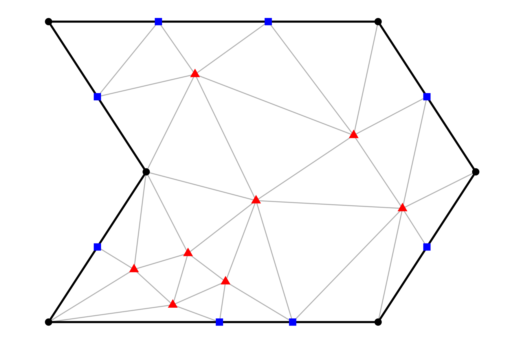
When constructing a CDT of $\Omega$, the constrained edges are chosen so as to preserve the domain boundary $\partial\Omega$. To fully specify these constraints and complete the triangulation, additional boundary vertices may be placed along $\partial\Omega$, and interior vertices can be introduced within $\Omega$ as needed. Specifically, let $\mathcal{V}_{\Omega}$ denote the vertex set of $\Omega$, and let $\mathcal{V}_{B}$ and $\mathcal{V}_{I}$ denote the additional vertices placed on $\partial\Omega$ and in $\Omega$, respectively. The constrained boundary edges are then generated from the vertex set $\mathcal{V}_{\Omega}\cup\mathcal{V}_{B}$ so as to coincide with $\partial\Omega$. The triangulation is completed by automatically generating the remaining edges to satisfy the visibility condition with respect to all vertices in $\mathcal{V}_{\Omega}\cup\mathcal{V}_{B}\cup\mathcal{V}_{I}$. Several efficient algorithms for obtaining CDTs are available (Chew, 1987; Wang and Schubert, 1987). In practice, CDTs can be easily constructed using convenient libraries. We use the Triangle library developed by Jonathan Shewchuk¹¹1https://www.cs.cmu.edu/~quake/triangle.html, available through the R package RTriangle. Figure 2 shows an example of a CDT for a polygon $\Omega$.

It is worth noting that a CDT is unique for a given vertex set under a mild genericity condition. As in the case of Delaunay triangulations, if the vertices are in general position, meaning that no four or more points are cocircular, then the resulting CDT is unique (Cheng et al., 2013, Theorem 2.18). When multiple CDTs are possible for a given vertex set, we resolve the ambiguity by deterministically selecting one in lexicographic order, following the implementation in the Triangle library. This tie-breaking rule ensures that the CDT mapping $(\partial\Omega,\mathcal{V}_{\Omega},\mathcal{V}_{B},\mathcal{V}_{I})\mapsto\Delta$ is well defined, so that the triangulation is uniquely specified once the vertex set is fixed. Consequently, our Bayesian procedure only needs to determine the vertex sets $\mathcal{V}_{B}$ and $\mathcal{V}_{I}$ for the triangulation. In what follows, we denote by $\Delta_{\Omega}^{\mathrm{CD}}(\mathcal{V}_{B},\mathcal{V}_{I})$ the CDT of $\Omega$ generated by $\mathcal{V}_{B}$ and set $\mathcal{V}_{I}$. For $\zeta>0$ and $\ell>0$, let $\mathcal{T}_{\Omega}^{\mathrm{CD}}(\zeta,\ell)$ be the collection of all such CDTs whose minimum angle is at least $\zeta$ and whose minimum edge length is at least $\ell$.

A CDT of $\Omega$ is determined by the vertex sets $(\mathcal{V}_{B},\mathcal{V}_{I})$. Thus, an appropriate choice of $\mathcal{V}_{B}$ and $\mathcal{V}_{I}$ is essential for obtaining a regular and adaptive triangulation. This choice should follow two main principles. First, the global complexity of the triangulation must balance approximation accuracy and model complexity. It should be large enough to provide an accurate approximation to $f_{0}$, but not so large as to impair computational efficiency or lead to overfitting. Second, the local placement of vertices determines the local resolution of the triangulation. Regions with smaller triangles provide greater local flexibility than regions with larger triangles, thereby allowing the spline estimator to adapt to spatial inhomogeneity.

Motivated by these principles, we treat both the number and locations of the vertices as unknown quantities and infer them from the data. This is naturally formulated in a Bayesian framework, where adaptivity can be induced through a prior distribution on the triangulation. A key ingredient is therefore a prior on $\mathcal{V}_{B}$ and $\mathcal{V}_{I}$ that controls the global complexity of the triangulation while allowing local refinement where the data support it. We specify this prior in the next section.

The true regression surface $f_{0}$ is approximated within $\mathcal{S}_{d}^{r}(\Delta)$. By the representation in (3), a prior on $\mathcal{S}_{d}^{r}(\Delta)$ is induced through priors for $(\Delta,\eta,\boldsymbol{\theta}_{\Delta})$. We first specify a prior over triangulations $\Delta\in\mathcal{T}_{\Omega}^{\mathrm{CD}}(\zeta,\ell)$ with given $\zeta>0$ and $\ell>0$. Since the CDT mapping $(\partial\Omega,\mathcal{V}_{\Omega},\mathcal{V}_{B},\mathcal{V}_{I})\mapsto\Delta_{\Omega}^{\mathrm{CD}}(\mathcal{V}_{B},\mathcal{V}_{I})$ is assumed to be well defined, it suffices to assign a prior to $(\mathcal{V}_{B},\mathcal{V}_{I})$.

Let $V_{B}=|\mathcal{V}_{B}|$ and $V_{I}=|\mathcal{V}_{I}|$. Let $\mu_{\partial\Omega}$ denote arclength measure on $\partial\Omega$ and let $\mu_{\Omega}$ denote Lebesgue measure on $\Omega$. We define the dominating measure $\mu_{\Omega}^{\oplus}=\sum_{v_{B}=0}^{\infty}\sum_{v_{I}=0}^{\infty}\mu_{\partial\Omega}^{v_{B}}\otimes\mu_{\Omega}^{v_{I}}$, on the disjoint union $\bigsqcup_{v_{B},v_{I}}(\partial\Omega)^{v_{B}}\times\Omega^{v_{I}}$, where the zeroth product measure is interpreted as the unit mass on the empty configuration. Define the admissible set of vertices,

We assign a prior to $(\mathcal{V}_{B},\mathcal{V}_{I})$ by specifying its density with respect to $\mu_{\Omega}^{\oplus}$ as

where $a_{B}(V_{B})=e^{-C_{B}V_{B}\log V_{B}}$ and $a_{I}(V_{I})=e^{-C_{I}V_{I}\log V_{I}}$ with prespecified constants $C_{B}>0$ and $C_{I}>0$. The omitted normalizing constant in (4) is independent of $(V_{B},V_{I})$ and cancels from all Metropolis-Hastings ratios. The factors $a_{B}$ and $a_{I}$ serve as a complexity penalty on the numbers of additional boundary and interior vertices. The induced marginal prior on $(V_{B},V_{I})$ is tilted by the admissible configuration volume. The induced prior distribution over $\mathcal{T}_{\Omega}^{\mathrm{CD}}(\zeta,\ell)$ is then given by the pushforward measure

Recall that the spline space is characterized by the basis representation in (3). To complete the prior specification on $\mathcal{S}_{d}^{r}(\Delta)$, we place a prior on the coefficients $(\eta,\boldsymbol{\theta}_{\Delta})$ conditional on the triangulation $\Delta$. The prior for $(\eta,\boldsymbol{\theta}_{\Delta})$ must be chosen carefully to reflect the model selection nature of the proposed framework (Moreno et al., 1998). The intercept $\eta$ is separated from the triangulation search and can be assigned a weakly informative prior. In contrast, a diffuse prior on $\boldsymbol{\theta}_{\Delta}$ is unsuitable because it may lead to Bartlett’s paradox (Bartlett, 1957). We therefore construct a prior for $\boldsymbol{\theta}_{\Delta}$ by combining a baseline coefficient-size penalty with a roughness penalty induced by the B-form representation.

Recall that under the linear constraints $\mathbf{H}_{\Delta}\boldsymbol{\gamma}_{\Delta}=0$ and $\mathbf{1}_{|\mathcal{B}_{\Delta}|}^{\mathsf{T}}\boldsymbol{\gamma}_{\Delta}=0$, the restricted spline $\mathcal{B}_{\Delta}(\cdot)^{\mathsf{T}}\boldsymbol{\gamma}_{\Delta}$ represents a function in $\mathcal{S}_{d}^{r}(\Delta)$ with the constant component removed. Since $\mathcal{B}_{\Delta}$ forms a partition of unity and hence has a comparable scale across its elements, a prior induced by the ridge penalty $\boldsymbol{\gamma}_{\Delta}^{\mathsf{T}}\boldsymbol{\gamma}_{\Delta}$ is reasonable to control the size of the spline $\mathcal{B}_{\Delta}(\cdot)^{\mathsf{T}}\boldsymbol{\gamma}_{\Delta}$. Since $\boldsymbol{\gamma}_{\Delta}=\tilde{\mathbf{Q}}_{\Delta}\boldsymbol{\theta}_{\Delta}$ and $\tilde{\mathbf{Q}}_{\Delta}^{\mathsf{T}}\tilde{\mathbf{Q}}_{\Delta}=\mathbf{I}_{J_{\Delta}}$, this leads to a Gaussian prior for $\boldsymbol{\theta}_{\Delta}$ with the quadratic term $\boldsymbol{\theta}_{\Delta}^{\mathsf{T}}\boldsymbol{\theta}_{\Delta}$. However, a coefficient-size penalty alone does not explicitly control the roughness of the fitted surface. Motivated by Lim et al. (2023), who observed that incorporating roughness penalization into a model selection prior can reduce the modeling bias induced by finite truncation, we augment the baseline ridge penalty with a roughness penalty. Following the triangulation literature (Lai and Wang, 2013; Yu et al., 2020), we employ the thin plate spline penalty of a function $f:\Omega\rightarrow\mathbb{R}$, given by

where $\nabla_{s_{j}}^{q}f$ denotes the $q$-th order derivative of $f$ in the direction of $s_{j}$ for $j=1,2$. The penalty applied to the spline $\mathcal{B}_{\Delta}(\cdot)^{\mathsf{T}}\boldsymbol{\gamma}_{\Delta}$ can be expressed as

for some $\mathbf{P}_{\Delta}\in\mathbb{R}^{|\mathcal{B}_{\Delta}|\times|\mathcal{B}_{\Delta}|}$ a block diagonal matrix whose blocks impose the penalty in (5) on the B-form over each $\tau\in\Delta$ (see the supplementary material for more details). By combining the two terms as a convex combination in the precision matrix, the proposed prior for $(\eta,\boldsymbol{\theta}_{\Delta})$ is given by

where $\kappa^{2}>0$ is a sufficiently large constant, $V_{\Delta}=|\mathcal{V}_{\Omega}|+|\mathcal{V}_{B}|+|\mathcal{V}_{I}|$ denotes the total number of vertices of the triangulation $\Delta$, $\lambda>0$ is a dispersion parameter, and $\nu\in(0,1)$ is a weight parameter that balances the two penalties. The factor $V_{\Delta}$ is introduced to appropriately scale the eigenvalues of $\tilde{\mathbf{Q}}_{\Delta}^{\mathsf{T}}\mathbf{P}_{\Delta}\tilde{\mathbf{Q}}_{\Delta}$ appropriately for the theoretical development, but it has little empirical effect. As $\nu\rightarrow 1$, the prior consists only of the term roughness penalty term on $\boldsymbol{\theta}_{\Delta}$. Conversely, as $\nu\rightarrow 0$, the prior reduces to ridge penalization on $\boldsymbol{\theta}_{\Delta}$.

To complete the prior specification, we assign priors with exponential tails on $\nu$ and $\lambda$, ensuring that for some $k>0$ and any increasing sequence $a_{n}>0$,

These tail properties are essential to satisfy the theoretical requirements. Note that an inverse-gamma prior for $\lambda$, despite its semi-conjugacy, does not satisfy (7) because of its polynomial right tail. Among priors with exponential tails, we adopt an exponential prior with rate $c_{\lambda}>0$ for $\lambda$. This choice yields a generalized inverse Gaussian conditional posterior for $\lambda$, thereby allowing convenient posterior updates. For $\nu$, computation can be efficiently performed using grid sampling for any prior distribution. To satisfy (7), we use a uniform prior on $(0,1-\delta_{\nu})$ with a small constant $\delta_{\nu}>0$. Lastly, for the variance parameter $\sigma^{2}$, we impose an inverse gamma prior,

with small $a_{\sigma}>0$ and $b_{\sigma}>0$. This specification is a natural choice because of its conjugacy, allowing complete marginalization in the posterior and thereby enabling efficient posterior updates for triangulations. Some additional technical difficulties arise from the polynomial tails of the induced marginal $t$-prior on $(\eta,\boldsymbol{\theta}_{\Delta})$. We address this issue by directly analyzing the marginal posterior of $\sigma^{2}$ and truncating regions with negligible posterior mass; see the supplementary material.

We first present the overall sampling steps. The priors introduced in Section 3 are carefully chosen to facilitate the construction of the sampler. As described, to meet the tail conditions in (7), we assign an exponential prior and a truncated uniform prior on $\lambda$ and $\nu$, respectively. Although an exponential prior for $\lambda$ is not conjugate, its monotone density enables a straightforward sampling scheme via data augmentation. For $\nu$, we employ grid sampling with efficiently evaluated density values at the specified grid points. We define $\mathbf{W}_{\Delta}=[\mathbf{1}_{n},\tilde{\mathbf{B}}_{\Delta}]\in\mathbb{R}^{n\times(J_{\Delta}+1)}$, where $\tilde{\mathbf{B}}_{\Delta}\in\mathbb{R}^{n\times J_{\Delta}}$ is the basis matrix with its $i$th row given by $\tilde{\mathcal{B}}_{\Delta}(\mathbf{s}_{i})$. We also define the block diagonal matrix $\boldsymbol{\Sigma}_{\Delta,\nu,\lambda}=\mathrm{diag}(\kappa^{2},\lambda(\nu V_{\Delta}^{-1}\tilde{\mathbf{Q}}_{\Delta}^{\mathsf{T}}\mathbf{P}_{\Delta}\tilde{\mathbf{Q}}_{\Delta}+(1-\nu)\mathbf{I}_{J_{\Delta}})^{-1})$. The following describes a blocked Gibbs sampler for exploring the posterior distribution.

1. (i)

   Draw $\Delta$ from $\pi(\Delta\mid\mathbf{y},\nu,\lambda)\propto\pi(\Delta)p(\mathbf{y}\mid\Delta,\nu,\lambda)$ using the birth-death-move proposals described in Section 4.2. The marginal likelihood $p(\mathbf{y}\mid\Delta,\nu,\lambda)$ is given by

   	$\displaystyle\textstyle p(\mathbf{y}\mid\Delta,\nu,\lambda)$	$\displaystyle\propto\Big\lvert\mathbf{I}_{J_{\Delta}+1}-\left(\mathbf{W}_{\Delta}^{\mathsf{T}}\mathbf{W}_{\Delta}+\boldsymbol{\Sigma}_{\Delta,\nu,\lambda}^{-1}\right)^{-1}\mathbf{W}_{\Delta}^{\mathsf{T}}\mathbf{W}_{\Delta}\Big\rvert^{1/2}$
   		$\displaystyle\quad\times\left[b_{\sigma}+\frac{1}{2}\Big(\mathbf{y}^{\mathsf{T}}\mathbf{y}-\mathbf{y}^{\mathsf{T}}\mathbf{W}_{\Delta}\left(\mathbf{W}_{\Delta}^{\mathsf{T}}\mathbf{W}_{\Delta}+\boldsymbol{\Sigma}_{\Delta,\nu,\lambda}^{-1}\right)^{-1}\mathbf{W}_{\Delta}^{\mathsf{T}}\mathbf{y}\Big)\right]^{-(a_{\sigma}+n/2)}.$

   The details of the Metropolis update are given in Section ?.

2. (ii)

   Draw $\sigma^{2}$ from $\pi(\sigma^{2}\mid\mathbf{y},\Delta,\nu,\lambda)$, which is

   $\displaystyle\text{IG}\!\left(a_{\sigma}+\frac{n}{2},b_{\sigma}+\frac{1}{2}\left(\mathbf{y}^{\mathsf{T}}\mathbf{y}-\mathbf{y}^{\mathsf{T}}\mathbf{W}_{\Delta}\left(\mathbf{W}_{\Delta}^{\mathsf{T}}\mathbf{W}_{\Delta}+\boldsymbol{\Sigma}_{\Delta,\nu,\lambda}^{-1}\right)^{-1}\mathbf{W}_{\Delta}^{\mathsf{T}}\mathbf{y}\right)\right).$

3. (iii)

   Draw $(\eta,\boldsymbol{\theta}_{\Delta})$ from $\pi(\eta,\boldsymbol{\theta}_{\Delta}\mid\mathbf{y},\Delta,\nu,\lambda,\sigma^{2})$, which is

   $\displaystyle\text{N}_{J_{\Delta}+1}\!\left(\left(\mathbf{W}_{\Delta}^{\mathsf{T}}\mathbf{W}_{\Delta}+\boldsymbol{\Sigma}_{\Delta,\nu,\lambda}^{-1}\right)^{-1}\mathbf{W}_{\Delta}^{\mathsf{T}}\mathbf{y},\sigma^{2}\!\left(\mathbf{W}_{\Delta}^{\mathsf{T}}\mathbf{W}_{\Delta}+\boldsymbol{\Sigma}_{\Delta,\nu,\lambda}^{-1}\right)^{-1}\right).$

4. (iv)

   Draw $\nu$ from $\pi(\nu\mid\mathbf{y},\Delta,\lambda,\sigma^{2},\eta,\boldsymbol{\theta}_{\Delta})\propto\pi(\nu)\pi(\boldsymbol{\theta}_{\Delta}\mid\Delta,\nu,\lambda,\sigma^{2})$ using grid sampling. Specifically,

   	$\displaystyle\pi(\boldsymbol{\theta}_{\Delta}\mid\Delta,\nu,\lambda,\sigma^{2})$	$\displaystyle\propto\nu^{{J_{\Delta}}/{2}}\prod_{k=1}^{J_{\Delta}}\left(\frac{\rho_{k}(\tilde{\mathbf{Q}}_{\Delta}^{\mathsf{T}}\mathbf{P}_{\Delta}\tilde{\mathbf{Q}}_{\Delta})}{V_{\Delta}}+\frac{1-\nu}{\nu}\right)^{1/2}$
   		$\displaystyle\quad\times\exp\left(-\frac{\nu}{2\lambda\sigma^{2}V_{\Delta}}\boldsymbol{\theta}_{\Delta}^{\mathsf{T}}\tilde{\mathbf{Q}}_{\Delta}^{\mathsf{T}}\mathbf{P}_{\Delta}\tilde{\mathbf{Q}}_{\Delta}\boldsymbol{\theta}_{\Delta}-\frac{1-\nu}{2\lambda\sigma^{2}}\boldsymbol{\theta}_{\Delta}^{\mathsf{T}}\boldsymbol{\theta}_{\Delta}\right),$

   where $\rho_{k}$ denotes the $k$th eigenvalue of the matrix. This sampling construction is highly efficient, as time-consuming operations such as eigen-decomposition and matrix multiplication need to be computed only once during the density evaluation.

5. (v)

   Draw $\lambda$ from $\pi(\lambda\mid\mathbf{y},\Delta,\nu,\sigma^{2},\eta,\boldsymbol{\theta}_{\Delta})$, which is

   $\displaystyle\lambda\mid\mathbf{y},\Delta,\nu,\sigma^{2},\eta,\boldsymbol{\theta}_{\Delta}$

   $\displaystyle\sim\text{GIG}\!\left(2c_{\lambda},\frac{\nu}{\sigma^{2}V_{\Delta}}\boldsymbol{\theta}_{\Delta}^{\mathsf{T}}\tilde{\mathbf{Q}}_{\Delta}^{\mathsf{T}}\mathbf{P}_{\Delta}\tilde{\mathbf{Q}}_{\Delta}\boldsymbol{\theta}_{\Delta}+\frac{1-\nu}{\sigma^{2}}\boldsymbol{\theta}_{\Delta}^{\mathsf{T}}\boldsymbol{\theta}_{\Delta},\frac{2-J_{\Delta}}{2}\right),$

   where $\mathrm{GIG}(a,b,p)$ denotes the generalized inverse Gaussian distribution with density proportional to $t\mapsto t^{p-1}\exp{-(at+b/t)/2}$ for $t>0$, where $a>0$, $b>0$, and $p\in\mathbb{R}$.

We first specify a proposal rule for updating triangulations over $\mathcal{T}_{\Omega}^{\mathrm{CD}}(\zeta,\ell)$. Since the CDT $\Delta_{\Omega}^{\mathrm{CD}}(\mathcal{V}_{B},\mathcal{V}_{I})$ is uniquely determined by the vertex sets $(\mathcal{V}_{B},\mathcal{V}_{I})$, updating $\Delta$ reduces to updating the vertices in $\mathcal{V}_{B}$ and $\mathcal{V}_{I}$. The corner vertices in $\mathcal{V}_{\Omega}$ are kept fixed throughout the Markov chain.

At each iteration, we choose one of the six proposal families

where $B^{+}$ and $I^{+}$ denote boundary and interior births, $B^{-}$ and $I^{-}$ denote boundary and interior deaths, and $B^{\leftrightarrow}$ and $I^{\leftrightarrow}$ denote boundary and interior moves. Let $p_{B^{+}}$, $p_{I^{+}}$, $p_{B^{-}}$, $p_{I^{-}}$, $p_{B^{\leftrightarrow}}$, $p_{I^{\leftrightarrow}}$ be the corresponding baseline probabilities. At the current state $\Delta$, unavailable proposal families are removed and the remaining probabilities are renormalized. Specifically, $B^{+}$ and $I^{+}$ are always available, $B^{-}$ and $B^{\leftrightarrow}$ are available only if $|\mathcal{V}_{B}|>0$, and $I^{-}$ and $I^{\leftrightarrow}$ are available only if $|\mathcal{V}_{I}|>0$. We denote the resulting state-dependent probability of selecting proposal family $a\in\mathcal{M}$ by

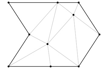
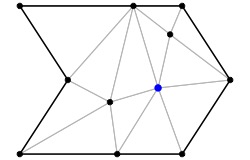
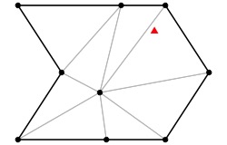
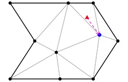
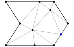
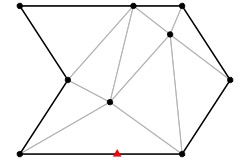
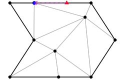
where $\mathcal{M}(\Delta)\subset\mathcal{M}$ is the set of proposal families available at $\Delta$. Each proposal is detailed below. Figure 3 provides a graphical illustration.

• •

  Boundary birth $(B^{+})$. A new boundary vertex is generated uniformly with respect to arclength measure on $\partial\Omega$. The proposal density is

  $$q(\Delta^{\prime}\mid\Delta)=\rho_{B^{+}}(\Delta)\frac{1}{|\partial\Omega|}.$$

• •

  Interior birth $(I^{+})$. A new interior vertex is generated uniformly over $\Omega$. The proposal density is

  $$q(\Delta^{\prime}\mid\Delta)=\rho_{I^{+}}(\Delta)\frac{1}{|\Omega|}.$$

• •

  Boundary death $(B^{-})$. This proposal is available only when $|\mathcal{V}_{B}|>0$. One boundary vertex is selected uniformly from $\mathcal{V}_{B}$ and removed. The proposal density is

  $$q(\Delta^{\prime}\mid\Delta)=\rho_{B^{-}}(\Delta)\frac{1}{|\mathcal{V}_{B}|}.$$

• •

  Interior death $(I^{-})$. This proposal is available only when $|\mathcal{V}_{I}|>0$. One interior vertex is selected uniformly from $\mathcal{V}_{I}$ and removed. The proposal density is

  $$q(\Delta^{\prime}\mid\Delta)=\rho_{I^{-}}(\Delta)\frac{1}{|\mathcal{V}_{I}|}.$$

• •

  Boundary move $(B^{\leftrightarrow})$. This proposal is available only when $|\mathcal{V}_{B}|>0$. One boundary vertex is selected uniformly from $\mathcal{V}_{B}$. Suppose the selected vertex $\mathbf{v}\in\mathcal{V}_{B}$ lies on boundary segment $[\mathbf{v}_{1},\mathbf{v}_{2}]$ and write $\mathbf{v}=(1-t)\mathbf{v}_{1}+t\mathbf{v}_{2}$ for $t\in(0,1)$. We draw $\delta$ from a uniform distribution on the interval $[-h_{B},h_{B}]$ and propose

  $$t^{\prime}=t+\delta,\qquad\mathbf{v}^{\prime}=(1-t^{\prime})\mathbf{v}_{1}+t^{\prime}\mathbf{v}_{2},$$

  where $h_{B}>0$ is a tuning parameter. If $t^{\prime}\notin(0,1)$, the proposal is rejected. Otherwise, the selected vertex $\mathbf{v}$ is moved to $\mathbf{v}^{\prime}$ and the CDT is recomputed. With respect to arclength measure on the boundary segment, the proposal density is

  $$q(\Delta^{\prime}\mid\Delta)=\rho_{B^{\leftrightarrow}}(\Delta)\frac{1}{|\mathcal{V}_{B}|}\times\frac{1}{2h_{B}\|\mathbf{v}_{1}-\mathbf{v}_{2}\|_{2}}.$$

  For admissible boundary moves, this proposal is symmetric.

• •

  Interior move $(I^{\leftrightarrow})$. This proposal is available only when $|\mathcal{V}_{I}|>0$. One interior vertex $\mathbf{v}$ is selected uniformly from $\mathcal{V}_{I}$. We draw uniformly $\mathbf{u}$ on the ball $\{\mathbf{z}\in\mathbb{R}^{2}:\|\mathbf{z}\|_{2}\leq r_{I}\}$ and propose $\mathbf{v}^{\prime}=\mathbf{v}+\mathbf{u}$. where $r_{I}>0$ is a tuning parameter. If $\mathbf{v}^{\prime}\notin\Omega$, the proposal is rejected. Otherwise, the selected vertex $\mathbf{v}$ is moved to $\mathbf{v}^{\prime}$ and the CDT is recomputed. The proposal density is

  $$q(\Delta^{\prime}\mid\Delta)=\rho_{I^{\leftrightarrow}}(\Delta)\frac{1}{|\mathcal{V}_{I}|}\frac{1}{\pi r_{I}^{2}}.$$

  For admissible interior moves, this proposal is symmetric.

Each proposed triangulation is accepted with probability

where $V_{B}=|\mathcal{V}_{B}|$, $V_{I}=|\mathcal{V}_{I}|$, $V^{\prime}_{B}=|\mathcal{V}^{\prime}_{B}|$, and $V^{\prime}_{I}=|\mathcal{V}^{\prime}_{I}|$, with the convention $0\log 0=0$. If the proposed triangulation is not admissible, the proposal is rejected.

We first show that the proposed method achieves a near-minimax posterior contraction rate under global Sobolev smoothness over $\Omega$. We assume that the true function $f_{0}$ belongs to the Sobolev space $\mathcal{W}^{m,\infty}$ for some $m\in\mathbb{N}$, so that all weak derivatives of $f_{0}$ up to order $m$ have finite $L^{\infty}$-norms. A key step in establishing the contraction rate is to construct an approximant of $f_{0}$ for which the prior places sufficient mass on a Kullback–Leibler neighborhood of $f_{0}$. Classical spline approximation theory implies that, for shape-regular triangulations, the approximation error is of order $L_{\Delta}^{m}$, where $L_{\Delta}$ is the maximum edge length of $\Delta$ (Lai and Schumaker, 1998). Since our prior controls triangulation complexity through the number of vertices rather than through the maximum edge length, we need to characterize the approximation resolution in terms of the number of vertices. To this end, we show that there exists a well-behaved vertex set such that, for the CDT $\Delta$ generated from any neighboring vertex set, $L_{\Delta}$ is of the same order as $V_{\Delta}^{-1/2}$; see the supplementary material.

Using this optimal approximator, we establish the posterior contraction rate through the standard argument based on prior concentration and suitable tests (Ghosal et al., 2000; Ghosal and van der Vaart, 2007). This argument requires a test function that is exponentially powerful with respect to the chosen metric. Although the Hellinger distance is well suited for constructing such tests (Le Cam, 1973; Birgé, 1983), its use in regression settings often requires relatively strong boundedness conditions (Ghosal and van der Vaart, 2007). To accommodate the unknown variance, we adopt the test function constructed by Jeong (2025), which employs a metric that jointly measures the discrepancy in the mean function and the variance parameter in Gaussian regression. Combining this test function with the entropy bound for a suitably chosen sieve yields the posterior contraction rate under the prior specified in Section 3. The proof is given in the supplementary material.

Theorem 1 shows that the posterior distribution contracts around the true parameter at the minimax rate for two-dimensional function estimation up to a logarithmic factor (Stone, 1982). The condition on $\zeta_{0}$ is mild because we can choose a sufficiently small positive minimum-angle threshold. The theoretical argument only needs $\zeta_{0}$ to be strictly positive, while the displayed upper bound ensures that the well-behaved CDT construction is contained in the support of the prior. The condition on $\ell_{n}$ requires the minimum admissible edge length to decrease at a suitable polynomial rate. It must decrease fast enough to allow the optimal approximating triangulation, but not so fast that the entropy bound becomes too large. Since $\ell_{n}$ is allowed to converge to zero at a sufficiently fast polynomial rate, this is merely a mild technical condition in practice.

Section 5.1 establishes optimal performance in a worst-case sense when the underlying function $f_{0}$ is globally regular. However, such a global smoothness result does not capture the ability of the proposed method to adapt to inhomogeneous or spatially varying features of $f_{0}$. In this section, we show that the proposed method indeed achieves ideal spatial adaptation in the sense of Donoho and Johnstone (1994). More precisely, although the prior is supported on CDTs, the resulting posterior contraction rate is governed by an oracle benchmark defined over an arbitrary class of triangulations of $\Omega$.

Let $\mathfrak{T}_{\Omega}$ be a collection of triangulations of $\Omega$. For $f_{0}:\Omega\rightarrow\mathbb{R}$, the benchmark oracle empirical $L^{2}$-risk is defined by

This quantity balances the approximation error of $f_{0}$ within the spline space $\mathcal{S}_{d}^{r}(\Delta)$ and the stochastic error associated with estimating the spline coefficients, with $J_{\Delta}$ serving as the dimension-based complexity penalty.

Unlike the minimax benchmark in Section 5.1, the oracle risk in (9) depends on the local and global features of the particular function $f_{0}$, and hence the benchmark reflects how well the triangulations in $\mathfrak{T}_{\Omega}$ can represent the spatial structure of $f_{0}$. In particular, the oracle may favor triangulations that allocate higher resolution to regions with localized features, while the penalty term $\sigma_{0}^{2}J_{\Delta}/n$ controls the total complexity of the resulting spline space. The oracle risk $R_{n}(f_{0};\mathfrak{T}_{\Omega})$ therefore provides a natural benchmark for procedures whose model class is restricted to $\mathfrak{T}_{\Omega}$. Because the triangulation prior is supported on $\mathcal{T}_{\Omega}^{\mathrm{CD}}(\zeta_{0},\ell_{n})$, the proposed method should ideally attain a near-oracle rate over a class of triangulations that closely reflects this support.

We identify the class of triangulations for which the proposed method attains near-optimality. For two finite point sets $\mathcal{V},\mathcal{V}^{\prime}\subset\mathbb{R}^{2}$ with $|\mathcal{V}|=|\mathcal{V}^{\prime}|$, define

where $\pi$ is a bijection. For vertex sets $\mathcal{V}_{B}\subset\partial\Omega$ and $\mathcal{V}_{I}\subset\Omega$, define

Let $\widetilde{\mathcal{T}}_{\Omega}^{\mathrm{CD}}(\zeta,\ell,\delta)$ be defined as the collection of triangulations $\Delta_{\Omega}^{\mathrm{CD}}(\mathcal{V}_{B},\mathcal{V}_{I})\in\mathcal{T}_{\Omega}^{\mathrm{CD}}(\zeta,\ell)$ such that, for every pair of vertex sets $(\mathcal{V}_{B}^{\prime},\mathcal{V}_{I}^{\prime})\in\mathfrak{V}_{\delta}(\mathcal{V}_{B},\mathcal{V}_{I})$, the perturbed CDT $\Delta_{\Omega}^{\mathrm{CD}}(\mathcal{V}_{B}^{\prime},\mathcal{V}_{I}^{\prime})$ satisfies $\Delta_{\Omega}^{\mathrm{CD}}(\mathcal{V}_{B}^{\prime},\mathcal{V}_{I}^{\prime})\in\mathcal{T}_{\Omega}^{\mathrm{CD}}(\zeta,\ell)$ and has the same combinatorial structure as $\Delta_{\Omega}^{\mathrm{CD}}(\mathcal{V}_{B},\mathcal{V}_{I})$. Hence, $\widetilde{\mathcal{T}}_{\Omega}^{\mathrm{CD}}(\zeta,\ell,\delta)$ consists of triangulations such that every $\delta$-perturbation of their vertex sets still induces a CDT in $\mathcal{T}_{\Omega}^{\mathrm{CD}}(\zeta,\ell)$ with the same combinatorial structure. By definition, $\widetilde{\mathcal{T}}_{\Omega}^{\mathrm{CD}}(\zeta,\ell,\delta)\subset\mathcal{T}_{\Omega}^{\mathrm{CD}}(\zeta,\ell)$, and we have $\widetilde{\mathcal{T}}_{\Omega}^{\mathrm{CD}}(\zeta,\ell,0)=\mathcal{T}_{\Omega}^{\mathrm{CD}}(\zeta,\ell)$. For small $\delta>0$, the robust core $\widetilde{\mathcal{T}}_{\Omega}^{\mathrm{CD}}(\zeta,\ell,\delta)$ may be viewed as a conservative inner approximation to $\mathcal{T}_{\Omega}^{\mathrm{CD}}(\zeta,\ell)$. It excludes triangulations lying too close to the boundary of the admissible class or to a change in CDT combinatorial structure, while retaining triangulations that are stable under small vertex perturbations.

The following theorem shows that the proposed method attains a near-oracle rate over this robust core. The proof is provided in the supplementary material.

The rate $r_{n}$ is slightly weaker than the oracle rate $R_{n}^{1/2}(f_{0};\mathcal{T}_{\Omega}^{\mathrm{CD}}(\zeta_{0},\ell_{n}))$. First, the approximation term is restricted to splines satisfying the uniform bound $\lVert f\rVert_{L^{\infty}}\leq B$. Second, the stochastic term contains an additional logarithmic factor. These two differences are mild because $f_{0}$ is assumed to be uniformly bounded and the logarithmic factor is negligible at the level of near-oracle rates. A more visible difference is that $r_{n}$ is defined over the perturbation-stable subcollection $\widetilde{\mathcal{T}}_{\Omega}^{\mathrm{CD}}(\zeta_{0},\ell_{n},\delta_{n})$ rather than over the entire CDT class $\mathcal{T}_{\Omega}^{\mathrm{CD}}(\zeta_{0},\ell_{n})$. This stability restriction is mild because $\delta_{n}$ decreases polynomially. Hence the robustness condition is imposed only against increasingly small vertex perturbations and becomes weaker as $n$ grows. Nevertheless, one might still worry that the proposed triangulation approach achieves near-optimality only over a restricted subset of the prior support. The following theorem shows that this is not the case. Up to constant losses in the shape-regularity parameters, the resulting rate is controlled by the near-oracle risk over arbitrary triangulations of $\Omega$ satisfying mild shape-regularity conditions. The proof is given in the supplementary material.