跳到论文正文
W Papers独立论文阅读器 arXiv:2606.10463 论文正文 计算阅读时间 · 0%
引用这篇论文根据当前论文元数据生成,正式投稿前建议核对。


License: arXiv.org perpetual non-exclusive license
arXiv:2606.10463v1 [math.ST] 09 Jun 2026

Distributionally Robust PCA with Data-Adaptive Wasserstein Geometry

Chuang Xu,    Andrew T. A. Wood and Yanrong Yang
Research School of Finance, Actuarial Studies and Statistics,
Australian National University
The authors are grateful to the Australian Research Council for supporting this research through grant DP220102232 
Abstract

We develop a distributionally robust formulation of principal component analysis that minimizes worst-case reconstruction risk over distributions lying within a Wasserstein neighborhood of the empirical measure. The Wasserstein neighborhood, viewed as an ambiguity set of distributions, is adaptively calibrated through a transport matrix GG to capture heterogeneous uncertainty across dimensions. The homogeneous case, in which GG is a scalar multiple of the identity matrix, recovers classical PCA. Under a general transport matrix GG, we derive a dual characterization of the associated minimax optimization problem and introduce a tractable surrogate objective function consisting of the square-root empirical reconstruction error plus a geometry-dependent residual exposure penalty. The exact and surrogate estimators are shown to be consistent for the population PCA subspace and asymptotically equivalent at the projector level. The transport geometry is allowed to be data adaptive, while the Wasserstein radius is calibrated via robust Wasserstein profile inference, yielding a data-driven radius of order n−1/2n^{-1/2}. Comprehensive theoretical guarantees are established, including consistency and local Grassmannian asymptotics exhibiting an explicit Wasserstein-induced drift determined by the limiting transport geometry and calibration level. Numerical experiments and a real-data application demonstrate that the proposed method can substantially improve finite-sample out-of-sample performance under structured covariance shifts, moderate contamination, and certain same-distribution regimes.

Keywords: Principal Component Analysis; Distributional Robust Optimisation; Wasserstein Distance; Adaptive Transport Geometry; Asymptotic theory.

1 Introduction

Principal component analysis (PCA) is one of the most widely used techniques for dimension reduction. It seeks a low-dimensional linear subspace that optimally represents the variation in original data, typically by maximizing explained variance or, equivalently, minimizing reconstruction error. Let X∈ℝpX\in\mathbb{R}^{p} be centered and the covariance matrix be Σ\Sigma, and if U∈𝕍p,r:={A∈ℝp×r:A⊤​A=Ir}U\in\mathbb{V}_{p,r}:=\{A\in\mathbb{R}^{p\times r}:A^{\top}A=I_{r}\} is an orthonormal basis for an rr-dimensional candidate principal subspace, then the population residual risk is

𝔼​{‖(Ip−U​U⊤)​X‖22}=tr⁡{Σ​(Ip−U​U⊤)}.\mathbb{E}\{\|(I_{p}-UU^{\top})X\|_{2}^{2}\}=\operatorname{tr}\{\Sigma(I_{p}-UU^{\top})\}.

In practice, PCA replaces the population covariance matrix Σ\Sigma with its sample counterpart Σ^n\widehat{\Sigma}_{n}. The asymptotic properties of the resulting estimator are well understood in the fixed-dimensional regime; see Anderson (1963), and extensive work has also studied in high-dimensional and functional settings (Johnstone and Lu 2009, Koltchinskii and Lounici 2017). Despite its optimality under the empirical distribution, ordinary PCA does not explicitly model uncertainty in the underlying data-generating mechanism. As a plug-in estimator based on the sample covariance matrix, it is inherently sensitive to sampling variability, contamination, and distributional shifts between the training and deployment environments. These issues are especially pronounced when eigengaps are small, when the covariance structure contains moderate spurious directions, or when future perturbations occur primarily in low-variance directions that are disregarded by classical PCA.

A substantial literature has developed robust alternatives to principal component analysis. Classical robust PCA methods either replace the empirical covariance matrix with a robust scatter estimator or define principal directions through projection pursuit. Early projection-pursuit approaches to robust dispersion matrices and principal components were introduced by Li and Chen (1985), while Croux and Haesbroeck (2000) studied PCA based on robust covariance and correlation estimators, including analyses of influence functions and efficiency. The ROBPCA procedure of Hubert et al. (2005), which combines projection pursuit with robust scatter estimation, has become a widely used method for outlier-resistant PCA. Another robustification strategy is based on Cauchy likelihood; see Fayomi et al. (2024). A different influential line of work uses the term robust PCA for low-rank-plus-sparse matrix decomposition. The seminal work of Candès et al. (2011) shows that a low-rank matrix can be exactly recovered from observations contaminated by sparse but potentially large corruptions. Robust PCA methods have also been developed for functional data; see, for example, the projection-pursuit approach of Bali et al. (2011). These contributions address important forms of robustness, including outliers, heavy tails, sparse corruptions and functional trajectory contamination. However, their primary objective is usually robust estimation of a covariance structure, a principal subspace, or a low-rank signal. In contrast, we aim to a general formulation which treats robustness as protection against a class of nearby distributions around the empirical distribution.

Distributionally robust optimization (DRO) provides a complementary robustness principle. Rather than replacing a sample quantity by a robust analogue, DRO optimizes the worst-case expected loss over an ambiguity set of probability distributions. Moment-based ambiguity sets were studied by Delage and Ye (2010), while Wasserstein ambiguity sets have become central in data-driven DRO because they provide a geometric framework for modelling distributional perturbations around the empirical distribution (Mohajerin Esfahani and Kuhn 2018, Blanchet and Murthy 2019, Gao and Kleywegt 2023). A key modelling choice is the transport cost, which determines the geometry of the ambiguity set. Most Wasserstein DRO formulations fix this geometry a priori and focus on tractability, guarantees, or radius calibration, whereas Blanchet et al. (2019a) show that learning transport costs can induce adaptive regularisation. This suggests that the ambiguity-set geometry may play an important statistical role: the radius controls the magnitude of distributional perturbations, while the transport cost determines which perturbation directions are considered plausible. Wasserstein DRO is closely connected to regularisation, generalisation and out-of-sample stability. For example, Wu et al. (2025a) establish broad regularisation and generalisation results, Gao et al. (2024) connect Wasserstein DRO with variation regularisation, and Gao (2023) study finite-sample guarantees. In portfolio optimisation, Blanchet et al. (2022a) develop a Wasserstein-robust mean–variance framework with data-driven uncertainty calibration, while related extensions consider high-dimensional factor portfolios (Wu et al. 2025b) and downside-risk optimisation under flexible risk measures and transport costs (Liu et al. 2026). More generally, dimensionality reduction has been proposed as a tool for improving tractability in high-dimensional DRO problems (Jiang et al. 2025). From a statistical perspective, robust Wasserstein profile inference (RWPI) calibrates Wasserstein ambiguity sets through profile statistics (Blanchet et al. 2019b), while related work develops confidence regions and asymptotic inference for Wasserstein DRO estimators (Blanchet et al. 2022b). More broadly, DRO has been linked to generalized empirical likelihood and uniform performance guarantees under distributional perturbations (Duchi et al. 2021, Duchi and Namkoong 2021).

A closely related contribution is Wang et al. (2025), who study PCA under a DRO formulation based on the standard Euclidean transport cost and show that it is equivalent to ordinary PCA. Motivated by this observation, we investigate the statistical role of anisotropic and data-adaptive transport geometry in Wasserstein DRO for PCA, together with RWPI-based radius calibration and local asymptotic analysis. Despite the growing DRO literature, statistically calibrated Wasserstein robustness for unsupervised PCA remains comparatively underexplored, particularly when the transport geometry is itself estimated from the data. The notion of robustness considered here differs from classical outlier resistance. Traditional robust PCA methods reduce the influence of atypical observations through robust scatter estimators, loss functions, or decomposition models. By contrast, distributional robustness treats the empirical distribution as a reference measure and seeks a subspace whose reconstruction risk remains controlled over a neighbourhood of nearby distributions. This reflects the broader distinction between classical robust statistics, which addresses data contamination, and DRO, which protects against distributional shifts between training and deployment environments (Blanchet et al. 2025). Ordinary PCA can also be sensitive to heterogeneous noise variances. For example, heteroskedastic PCA corrects coordinate-dependent noise in spiked covariance models (Zhang et al. 2022). By contrast, the transport geometry in our Wasserstein DRO formulation encodes heterogeneous distributional uncertainty rather than variance heterogeneity, providing robustness to distributional perturbations beyond classical heteroscedastic modelling.

This gap is not merely a matter of extending an existing Wasserstein DRO construction to an unsupervised setting. Under the standard Euclidean transport cost, the Wasserstein ambiguity set represents homogeneous uncertainty across directions, and the resulting robust optimization problem preserves the classical PCA ordering of subspaces. This observation shifts the focus from the size of the Wasserstein ambiguity set to its geometry. While the Euclidean transport cost provides a natural homogeneous-uncertainty benchmark, it is incapable of producing a non-trivial robustification of PCA. The relevant statistical object is therefore the transport geometry itself. We propose to model this geometry through a positive definite transport matrix GG, which specifies the relative cost of perturbations in different directions and thereby encodes heterogeneous distributional uncertainty. The induced Wasserstein DRO criterion regularizes PCA by controlling residual exposure along uncertainty-sensitive directions, while a locally calibrated Wasserstein radius captures the overall scale of uncertainty.

This paper develops a weighted Wasserstein DRO formulation of PCA. Let X1,…,Xn∈ℝpX_{1},\ldots,X_{n}\in\mathbb{R}^{p} be centred observations and write ℙ^n=1n​∑i=1nδXi,Σ^n=1n​∑i=1nXi​Xi⊤.\widehat{\mathbb{P}}_{n}=\frac{1}{n}\sum_{i=1}^{n}\delta_{X_{i}},\widehat{\Sigma}_{n}=\frac{1}{n}\sum_{i=1}^{n}X_{i}X_{i}^{\top}. For a candidate rank-rr principal basis U∈𝕍p,rU\in\mathbb{V}_{p,r}, let ΠU:=U​U⊤,QU:=Ip−ΠU,\Pi_{U}:=UU^{\top},Q_{U}:=I_{p}-\Pi_{U}, where ΠU\Pi_{U} is the principal projector and QUQ_{U} is the residual projector of rank s=p−rs=p-r. For a positive definite matrix GG, define the weighted quadratic transport cost cG​(x,y)=(x−y)⊤​G​(x−y),c_{G}(x,y)=(x-y)^{\top}G(x-y), and let W2,GW_{2,G} be the corresponding Wasserstein distance, defined below in (2). For Q∈𝒢sQ\in\mathcal{G}_{s}, where 𝒢s\mathcal{G}_{s} denotes the Grassmannian represented as rank-ss orthogonal projectors, we define the exact robust residual risk

Φn,δG​(Q):=supℙ:W2,G​(ℙ,ℙ^n)≤δ𝔼Z∼ℙ​(Z⊤​Q​Z).\Phi_{n,\delta}^{G}(Q):=\sup_{\mathbb{P}:\,W_{2,G}(\mathbb{P},\widehat{\mathbb{P}}_{n})\leq\delta}\mathbb{E}_{Z\sim\mathbb{P}}(Z^{\top}QZ).

The weighted Wasserstein DRO-PCA problem is then to minimise Φn,δG​(Q)\Phi_{n,\delta}^{G}(Q) over Q∈𝒢sQ\in\mathcal{G}_{s}.

The Euclidean transport cost provides a natural benchmark corresponding to homogeneous uncertainty across directions. In this case, Wasserstein robustification is degenerate for PCA: the exact worst-case reconstruction risk is a monotone transformation of the empirical reconstruction error and therefore yields exactly the same principal subspace. A related equivalence result for Euclidean Wasserstein DRO-PCA was obtained by Wang et al. (2025). Consequently, the key modelling ingredient is not the Wasserstein radius but the transport geometry. The positive definite matrix GG governs this geometry by determining which perturbation directions are relatively inexpensive for the adversary, thereby controlling how robustness reshapes the fitted subspace. The relevant directional quantity is the residual exposure ρG​(Q):=λmax​{G−1/2​Q​G−1/2}.\rho_{G}(Q):=\lambda_{\max}\{G^{-1/2}QG^{-1/2}\}. Directions that are inexpensive under the transport cost are amplified by G−1/2G^{-1/2}. Residual subspaces aligned with such directions therefore have larger worst-case exposure. Wasserstein duality yields an exact dual representation of Φn,δG\Phi_{n,\delta}^{G} and motivates the tractable surrogate criterion

𝒥n,δG​(Q):=tr⁡(Σ^n​Q)+δ​ρG​(Q).\displaystyle\mathcal{J}_{n,\delta}^{G}(Q):=\sqrt{\operatorname{tr}(\widehat{\Sigma}_{n}Q)}+\delta\sqrt{\rho_{G}(Q)}. (1)

The first term is the square root empirical reconstruction error, while the second term is a geometry-dependent exposure penalty. A key feature of this formulation is that the transport matrix GG is not merely a technical device. It determines which perturbation directions are inexpensive for the adversary and therefore which residual directions are penalised by the DRO criterion. While much of the Wasserstein DRO literature focuses on the ambiguity radius, the choice of the transport cost is itself a modelling problem. We therefore allow the geometry to be estimated from the data, writing G^n\widehat{G}_{n}, and develop the theory under general operator-norm consistency and spectral stability conditions.

The second ingredient is data-driven calibration of the Wasserstein radius. The radius δ\delta should be large enough to reflect sampling uncertainty, but not so large that the adversarial term dominates the empirical reconstruction term. We calibrate the radius through an RWPI statistic associated with the PCA first-order condition. For a data-adaptive transport matrix G^n\widehat{G}_{n}, the RWPI statistic is defined as the smallest squared W2,G^nW_{2,\widehat{G}_{n}}-perturbation of the empirical distribution under which the defined estimating equation holds at the population subspace. Its limiting law determines a radius δ^n,α\widehat{\delta}_{n,\alpha} of order n−1/2n^{-1/2}. This calibration places the robustification on the local statistical scale: the Wasserstein penalty is asymptotically small enough to preserve the population PCA target, but large enough to affect the root-nn local behaviour of the fitted subspace.

Note that the proposed method is designed to achieve distributional robustness in local neighborhood of the empirical distribution, defined in terms of the Wasserstein distance. Distributional robustness does not include robustness against distributions with arbitrarily heavy tails , because the Wasserstein distance (2) does not remain bounded in this setting. Nevertheless, the proposed framework achieves distributional robustness over a broad class of local perturbations characterized by bounded Wasserstein distance from the reference distribution, thereby providing protection against a wide range of realistic model mis-specifications.

The main contributions of the paper are as follows.

  1. (i)

    Methodology. We formulate PCA as a weighted Wasserstein DRO problem with transport matrix GG. The transport geometry encodes heterogeneous distributional uncertainty, and Euclidean geometry is shown to be degenerate for PCA. For general GG, we derive a dual representation of the robust risk and an interpretable upper bound, leading to the surrogate objective (1), which provides a tractable directional regularization of PCA.

  2. (ii)

    Data-adaptivity. We introduce a data-adaptive transport geometry G^n\widehat{G}_{n} together with an RWPI-calibrated radius δ^n,α\widehat{\delta}_{n,\alpha}. Under operator-norm consistency and spectral stability of G^n\widehat{G}_{n}, the adaptive profile statistic converges to a weighted chi-square distribution. This yields a fully data-driven radius calibration that avoids cross-validation and externally specified regularization parameters.

  3. (iii)

    Theory. Fundamental asymptotic theory is established on the Grassmannian. The exact adaptive DRO estimator is consistent, while the adaptive surrogate estimator satisfies a root-nn projector central limit theorem. Relative to classical PCA, the limiting distribution contains an explicit Wasserstein-induced drift determined by the transport geometry and RWPI calibration.

  4. (iv)

    Finite-sample performance. We evaluate the proposed method through simulations and real-data analysis. Across settings involving out-of-sample reconstruction, covariance shift, training contamination, and image-region transfer, the results show that adaptive Wasserstein geometry can improve reconstruction when aligned with the underlying perturbation structure. The experiments identify the settings in which calibrated Wasserstein regularization is most beneficial.

In the numerical studies, we consider two diagonal data-adaptive transport geometries. The first, a residual-variance geometry, assigns lower transport cost to coordinates with large variation unexplained by an initial PCA fit. The second, a PCA-block variance geometry, assigns lower transport cost to coordinates with large variation captured by the leading empirical principal components. These choices reflect different assumptions about whether target-relevant directions lie in the residual or PCA subspace. More generally, the theory applies to any adaptive transport geometry G^n\widehat{G}_{n} that converges in operator norm to a positive definite limit. The transport geometry can therefore be chosen to incorporate domain knowledge about plausible distributional perturbations.

For a matrix AA, ‖A‖op\|A\|_{\operatorname{op}} and ‖A‖F\|A\|_{F} denote the operator and Frobenius norms. If AA is a symmetric matrix, λmin​(A)\lambda_{\min}(A) and λmax​(A)\lambda_{\max}(A) denote its smallest and largest eigenvalues; A⪰0A\succeq 0 means that AA is positive semidefinite; and A⪯BA\preceq B means B−A⪰0B-A\succeq 0. Convergence in probability and convergence in distribution are denoted by →𝑝\xrightarrow{p} and ⇒\Rightarrow, respectively, and equality in distribution by =𝑑\overset{d}{=}. We use Op​(⋅)O_{p}(\cdot) and op​(⋅)o_{p}(\cdot) in their usual stochastic-order senses. We write A=Op​(⋅)A=O_{p}(\cdot) or A=op​(⋅)A=o_{p}(\cdot) for a matrix AA, if ‖A‖F=Op​(⋅)||A||_{F}=O_{p}(\cdot) or ‖A‖F=op​(⋅)||A||_{F}=o_{p}(\cdot), respectively.

The rest of the paper is organised as follows. Section 2 introduces the weighted Wasserstein DRO-PCA formulation, records the Euclidean degeneracy result in our formulation, and derives the surrogate criterion. Section 3 develops the RWPI calibration of the Wasserstein radius under an adaptive transport metric. Section 4 gives the consistency, local quadratic expansion, and Grassmannian central limit theorem for the adaptive surrogate estimator. Section 5 discusses practical choices of the transport geometry and summarises the adaptive DRO-PCA implementation. Section 6 reports simulation and Section 7 reports real-data evidence. The supplementary material contains proofs and additional numerical details.

2 A weighted Wasserstein formulation of DRO-PCA

Let X1,…,Xn∈ℝpX_{1},\ldots,X_{n}\in\mathbb{R}^{p} be centred observations, and write ℙ^n:=1n​∑i=1nδXi,Σ^n:=1n​∑i=1nXi​Xi⊤.\widehat{\mathbb{P}}_{n}:=\frac{1}{n}\sum_{i=1}^{n}\delta_{X_{i}},\widehat{\Sigma}_{n}:=\frac{1}{n}\sum_{i=1}^{n}X_{i}X_{i}^{\top}.

Remark 1.

Throughout the paper we assume, for notational convenience, that the observations have been centred. If the raw observations are not centred, the procedure may be applied after empirical centring. This empirical centring has asymptotically negligible effect on all of our results under suitable moment conditions.

For m∈{1,…,p−1}m\in\{1,\ldots,p-1\}, let 𝒢m:={Q∈ℝp×p:Q⊤=Q,Q2=Q,tr⁡(Q)=m}\mathcal{G}_{m}:=\{Q\in\mathbb{R}^{p\times p}:Q^{\top}=Q,\ Q^{2}=Q,\ \operatorname{tr}(Q)=m\} denote the Grassmannian represented as rank-mm orthogonal projectors. We fix a target principal dimension r<pr<p, set s:=p−rs:=p-r, and write

𝕍p,r:={U∈ℝp×r:U⊤​U=Ir},ΠU:=U​U⊤,QU:=Ip−ΠU.\mathbb{V}_{p,r}:=\{U\in\mathbb{R}^{p\times r}:U^{\top}U=I_{r}\},\qquad\Pi_{U}:=UU^{\top},\qquad Q_{U}:=I_{p}-\Pi_{U}.

Thus ΠU∈𝒢r\Pi_{U}\in\mathcal{G}_{r} is the candidate principal projector and QU∈𝒢sQ_{U}\in\mathcal{G}_{s} is its residual projector. Classical PCA solves minU∈𝕍p,r⁡tr⁡(Σ^n​QU),\min_{U\in\mathbb{V}_{p,r}}\operatorname{tr}(\widehat{\Sigma}_{n}Q_{U}), or equivalently maximises tr⁡(Σ^n​ΠU)\operatorname{tr}(\widehat{\Sigma}_{n}\Pi_{U}).

The distributionally robust version replaces the empirical reconstruction error by a worst-case reconstruction error over a neighbourhood of the empirical law. For a symmetric positive definite matrix GG, define ‖x‖G2:=x⊤​G​x,cG​(x,y):=‖x−y‖G2,\|x\|_{G}^{2}:=x^{\top}Gx,c_{G}(x,y):=\|x-y\|_{G}^{2}, and let W2,GW_{2,G} be the corresponding Wasserstein distance,

W2,G​(μ,ν)≔(infπ∈Π​(μ,ν)∫‖x−y‖G2​dπ​(x,y))1/2,W_{2,G}(\mu,\nu)\coloneqq\left(\inf_{\pi\in\Pi(\mu,\nu)}\int\|x-y\|_{G}^{2}\,\mathrm{d}\pi(x,y)\right)^{1/2}, (2)

where Π​(μ,ν)\Pi(\mu,\nu) denotes the set of couplings of μ\mu and ν\nu. The weighted Wasserstein ambiguity set is 𝒰δG​(ℙ^n):={ℙ:W2,G​(ℙ,ℙ^n)≤δ}.\mathcal{U}_{\delta}^{G}(\widehat{\mathbb{P}}_{n}):=\{\mathbb{P}:W_{2,G}(\mathbb{P},\widehat{\mathbb{P}}_{n})\leq\delta\}. Throughout, when writing 𝔼ℙ​f​(Z)\mathbb{E}_{\mathbb{P}}f(Z), we understand ZZ to be distributed according to ℙ\mathbb{P}. For Q∈𝒢sQ\in\mathcal{G}_{s}, define the exact robust residual risk

Φn,δG​(Q):=supℙ∈𝒰δG​(ℙ^n)𝔼ℙ​(Z⊤​Q​Z).\Phi_{n,\delta}^{G}(Q):=\sup_{\mathbb{P}\in\mathcal{U}_{\delta}^{G}(\widehat{\mathbb{P}}_{n})}\mathbb{E}_{\mathbb{P}}(Z^{\top}QZ). (3)

The weighted Wasserstein DRO-PCA problem is then

infQ∈𝒢sΦn,δG​(Q)=infU∈𝕍p,rsupℙ∈𝒰δG​(ℙ^n)𝔼ℙ​{‖QU​Z‖22}.\inf_{Q\in\mathcal{G}_{s}}\Phi_{n,\delta}^{G}(Q)=\inf_{U\in\mathbb{V}_{p,r}}\sup_{\mathbb{P}\in\mathcal{U}_{\delta}^{G}(\widehat{\mathbb{P}}_{n})}\mathbb{E}_{\mathbb{P}}\{\|Q_{U}Z\|_{2}^{2}\}. (4)

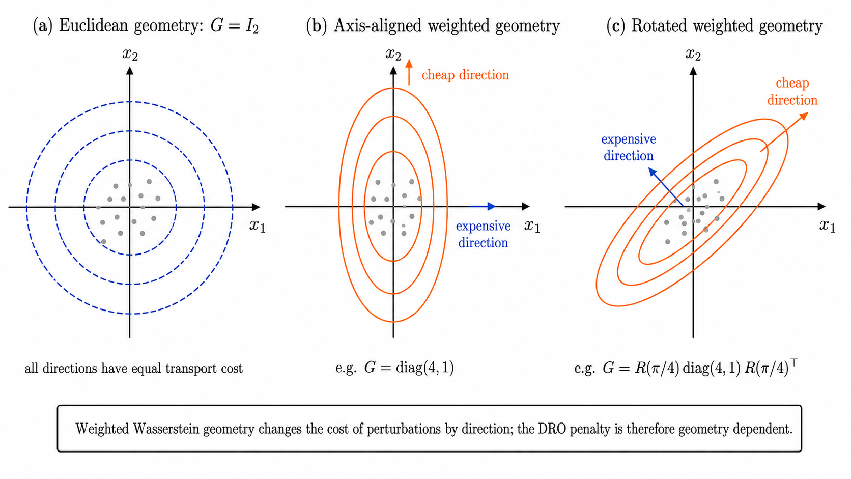
This formulation separates two choices: the radius δ\delta, which determines the size of the ambiguity set, and the matrix GG, which determines the geometry of admissible distributional perturbations. Figure 1 gives a two-dimensional schematic of the role of GG: changing GG changes the directions in which Wasserstein perturbations are cheap or expensive.
Refer to caption
Figure 1: Schematic illustration of the weighted Wasserstein transport geometry. Panel (a) shows the Euclidean case G=I2G=I_{2}, where all directions have the same transport cost. Panel (b) illustrates an axis-aligned weighted geometry, for example G=diag⁡(4,1)G=\operatorname{diag}(4,1), where perturbations in the second coordinate direction are cheaper. Panel (c) illustrates a rotated weighted geometry, for example G=R​(π/4)​diag⁡(4,1)​R​(π/4)⊤G=R(\pi/4)\operatorname{diag}(4,1)R(\pi/4)^{\top}, where the cheap and expensive perturbation directions are determined by the eigenvectors of GG. The figure illustrates that the matrix GG changes the cost of perturbations by direction.

The following theorem characterizes the homogeneous-geometry benchmark in our distributionally robust framework. Under the standard Euclidean transport geometry, the Wasserstein robust objective is equivalent to classical PCA and therefore induces the same ordering of subspaces. Related equivalence results for Euclidean Wasserstein DRO-PCA were also established by Wang et al. (2025). In the Euclidean case G=IpG=I_{p}, we write W2:=W2,IpW_{2}:=W_{2,I_{p}}.

Theorem 1.

Let X1,…,Xn∈ℝpX_{1},\ldots,X_{n}\in\mathbb{R}^{p} be centred observations, define ℙ^n=n−1​∑i=1nδXi,Σ^n=n−1​∑i=1nXi​Xi⊤,\widehat{\mathbb{P}}_{n}=n^{-1}\sum_{i=1}^{n}\delta_{X_{i}},\widehat{\Sigma}_{n}=n^{-1}\sum_{i=1}^{n}X_{i}X_{i}^{\top}, and let 1≤r<p1\leq r<p. Let 𝒫2​(ℝp)\mathcal{P}_{2}(\mathbb{R}^{p}) denote the set of probability measures on ℝp\mathbb{R}^{p} with finite second moment. For every δ≥0\delta\geq 0 and every U∈𝕍p,rU\in\mathbb{V}_{p,r},

supℙ∈𝒫2​(ℝp):W2​(ℙ,ℙ^n)≤δ𝔼ℙ​{‖QU​Z‖22}={tr⁡(Σ^n​QU)+δ}2.\sup_{\mathbb{P}\in\mathcal{P}_{2}(\mathbb{R}^{p}):W_{2}(\mathbb{P},\widehat{\mathbb{P}}_{n})\leq\delta}\mathbb{E}_{\mathbb{P}}\{\|Q_{U}Z\|_{2}^{2}\}=\left\{\sqrt{\operatorname{tr}(\widehat{\Sigma}_{n}Q_{U})}+\delta\right\}^{2}.

Consequently,

arg​minU∈𝕍p,r​supℙ∈𝒫2​(ℝp):W2​(ℙ,ℙ^n)≤δ𝔼ℙ​{‖QU​Z‖22}=arg​minU∈𝕍p,r⁡tr⁡(Σ^n​QU).\operatorname*{arg\,min}_{U\in\mathbb{V}_{p,r}}\sup_{\mathbb{P}\in\mathcal{P}_{2}(\mathbb{R}^{p}):W_{2}(\mathbb{P},\widehat{\mathbb{P}}_{n})\leq\delta}\mathbb{E}_{\mathbb{P}}\{\|Q_{U}Z\|_{2}^{2}\}=\operatorname*{arg\,min}_{U\in\mathbb{V}_{p,r}}\,\operatorname{tr}(\widehat{\Sigma}_{n}Q_{U}).
Remark 2.

Theorem 1 shows that Euclidean Wasserstein robustification applies a monotone transformation to the empirical reconstruction error and therefore preserves the ordinary PCA ordering of subspaces. Thus, classical PCA arises as a special case of Wasserstein DRO corresponding to a homogeneous transport geometry, where all perturbation directions are treated symmetrically. The weighted Wasserstein formulation considered here generalizes this benchmark by introducing a positive definite transport matrix GG that specifies an anisotropic geometry of distributional uncertainty and permits distributional robustness to act differently across directions.

We now return to a general positive definite matrix GG. The role of GG is most clearly seen through the residual exposure operator

𝖲G​(Q):=G−1/2​Q​G−1/2,ρG​(Q):=λmax​{𝖲G​(Q)},Q∈𝒢s.\displaystyle\mathsf{S}_{G}(Q):=G^{-1/2}QG^{-1/2},\qquad\rho_{G}(Q):=\lambda_{\max}\{\mathsf{S}_{G}(Q)\},\qquad Q\in\mathcal{G}_{s}. (5)

We also write Σ~n,G:=G1/2​Σ^n​G1/2\widetilde{\Sigma}_{n,G}:=G^{1/2}\widehat{\Sigma}_{n}G^{1/2}. The exposure term can be understood through the Rayleigh–Ritz characterisation ρG​(Q)=sup‖v‖2=1v⊤​G−1/2​Q​G−1/2​v.\rho_{G}(Q)=\sup_{\|v\|_{2}=1}v^{\top}G^{-1/2}QG^{-1/2}v. For example, if G=diag⁡(g1,…,gp)G=\operatorname{diag}(g_{1},\ldots,g_{p}), then for the jjth standard coordinate vector eje_{j},

ρG​(Q)≥gj−1​ej⊤​Q​ej=gj−1​‖Q​ej‖22.\rho_{G}(Q)\geq g_{j}^{-1}e_{j}^{\top}Qe_{j}=g_{j}^{-1}\|Qe_{j}\|_{2}^{2}.

Thus a coordinate with small transport cost gjg_{j} receives a large penalty if it has substantial projection onto the residual subspace. The surrogate (6) defined later therefore encourages the fitted principal subspace to capture directions that are inexpensive for the adversary to perturb. By standard Wasserstein DRO duality (e.g. Blanchet and Murthy 2019, Gao and Kleywegt 2023), followed by a direct quadratic calculation, we obtain

Φn,δG​(Q)=infλ>ρG​(Q)[λ​δ2+λ​tr⁡{Σ~n,G​𝖲G​(Q)​(λ​Ip−𝖲G​(Q))−1}],\Phi_{n,\delta}^{G}(Q)=\inf_{\lambda>\rho_{G}(Q)}\left[\lambda\delta^{2}+\lambda\operatorname{tr}\left\{\widetilde{\Sigma}_{n,G}\mathsf{S}_{G}(Q)\bigl(\lambda I_{p}-\mathsf{S}_{G}(Q)\bigr)^{-1}\right\}\right],

with the detailed derivation given in Supplementary Section 10.2. Although this dual representation is exact, it is most useful for our purposes because it makes explicit how the empirical second moment Σ~n,G\widetilde{\Sigma}_{n,G} interacts with 𝖲G​(Q)\mathsf{S}_{G}(Q). To obtain a tractable criterion, we bound the resolvent term by its worst spectral value. Since the eigenvalues of 𝖲G​(Q)\mathsf{S}_{G}(Q) are bounded above by ρG​(Q)\rho_{G}(Q), for λ>ρG​(Q)\lambda>\rho_{G}(Q),

𝖲G​(Q)​{λ​Ip−𝖲G​(Q)}−1⪯1λ−ρG​(Q)​𝖲G​(Q).\mathsf{S}_{G}(Q)\{\lambda I_{p}-\mathsf{S}_{G}(Q)\}^{-1}\preceq\frac{1}{\lambda-\rho_{G}(Q)}\mathsf{S}_{G}(Q).

Together with tr⁡{Σ~n,G​𝖲G​(Q)}=tr⁡(Σ^n​Q),\operatorname{tr}\{\widetilde{\Sigma}_{n,G}\mathsf{S}_{G}(Q)\}=\operatorname{tr}(\widehat{\Sigma}_{n}Q), this reduces the exact dual objective to a one-dimensional upper envelope depending only on the empirical reconstruction error and the residual exposure ρG​(Q)\rho_{G}(Q). Optimising this envelope over λ\lambda gives the following bound.

Theorem 2.

Let X1,…,Xn∈ℝpX_{1},\ldots,X_{n}\in\mathbb{R}^{p} be centred observations, let ℙ^n=n−1​∑i=1nδXi\widehat{\mathbb{P}}_{n}=n^{-1}\sum_{i=1}^{n}\delta_{X_{i}}, Σ^n=n−1​∑i=1nXi​Xi⊤\widehat{\Sigma}_{n}=n^{-1}\sum_{i=1}^{n}X_{i}X_{i}^{\top}, let G be symmetric positive definite matrix, and let δ≥0\delta\geq 0. Then, for every Q∈𝒢sQ\in\mathcal{G}_{s},

Φn,δG​(Q)≤{tr⁡(Σ^n​Q)+δ​ρG​(Q)}2,\Phi_{n,\delta}^{G}(Q)\leq\left\{\sqrt{\operatorname{tr}(\widehat{\Sigma}_{n}Q)}+\delta\sqrt{\rho_{G}(Q)}\right\}^{2},

where ρG​(Q)\rho_{G}(Q) is defined in (5).

Theorem 2 shows that, unlike the Euclidean case, the transport geometry now affects the relative ranking of residual subspaces through ρG​(Q)\rho_{G}(Q), thereby inducing a genuine regularisation effect.

The bound in Theorem 2 suggests the surrogate criterion

𝒥n,δG​(Q):=tr⁡(Σ^n​Q)+δ​ρG​(Q),Q∈𝒢s.\mathcal{J}_{n,\delta}^{G}(Q):=\sqrt{\operatorname{tr}(\widehat{\Sigma}_{n}Q)}+\delta\sqrt{\rho_{G}(Q)},\qquad Q\in\mathcal{G}_{s}. (6)

Since the map x↦x2x\mapsto x^{2} is increasing on [0,∞)[0,\infty), minimising 𝒥n,δG​(Q)\mathcal{J}_{n,\delta}^{G}(Q) is equivalent to minimising the upper bound in Theorem 2. We therefore use 𝒥n,δG\mathcal{J}_{n,\delta}^{G} as the tractable criterion for computation and for the local asymptotic analysis developed below. Numerical implementation details are given in Supplementary Section 14.

When GG is clear from context, we write 𝒥n,δ\mathcal{J}_{n,\delta} for 𝒥n,δG\mathcal{J}_{n,\delta}^{G}. The two terms in (6) have distinct statistical meanings. The first is the square root empirical reconstruction error, and therefore favours the ordinary PCA residual subspace. The second penalises residual subspaces that are aligned with low-cost transport directions. In this sense, the surrogate does not merely inflate the PCA criterion; it introduces a directional regularisation determined by the transport geometry.

Remark 3.

If G=IpG=I_{p}, then 𝖲G​(Q)=Q\mathsf{S}_{G}(Q)=Q and ρG​(Q)=1\rho_{G}(Q)=1 for every Q∈𝒢sQ\in\mathcal{G}_{s} so the surrogate minimisers coincide with ordinary PCA, consistent with Theorem 1.

It is important to distinguish the exact criterion Φn,δG\Phi_{n,\delta}^{G} from the surrogate criterion 𝒥n,δG\mathcal{J}_{n,\delta}^{G}. The former is the genuine Wasserstein worst-case reconstruction risk, whereas the latter is the tractable spectral criterion used for computation and local asymptotic analysis. We do not claim that the two criteria have identical finite-sample minimisers.

Remark 4.

Let Qsur∈arg​minQ∈𝒢s⁡𝒥n,δG​(Q),Qex∈arg​minQ∈𝒢s⁡Φn,δG​(Q).Q_{\mathrm{sur}}\in\operatorname*{arg\,min}_{Q\in\mathcal{G}_{s}}\mathcal{J}_{n,\delta}^{G}(Q),\quad Q_{\mathrm{ex}}\in\operatorname*{arg\,min}_{Q\in\mathcal{G}_{s}}\Phi_{n,\delta}^{G}(Q). Since Φn,δG​(Q)≤{𝒥n,δG​(Q)}2\Phi_{n,\delta}^{G}(Q)\leq\{\mathcal{J}_{n,\delta}^{G}(Q)\}^{2} for every Q∈𝒢sQ\in\mathcal{G}_{s}, optimality gives

0\displaystyle 0 ≤Φn,δG​(Qsur)−Φn,δG​(Qex)≤{𝒥n,δG​(Qex)}2−Φn,δG​(Qex)≤supQ∈𝒢s[{𝒥n,δG​(Q)}2−Φn,δG​(Q)].\displaystyle\leq\Phi_{n,\delta}^{G}(Q_{\mathrm{sur}})-\Phi_{n,\delta}^{G}(Q_{\mathrm{ex}})\leq\{\mathcal{J}_{n,\delta}^{G}(Q_{\mathrm{ex}})\}^{2}-\Phi_{n,\delta}^{G}(Q_{\mathrm{ex}})\leq\sup_{Q\in\mathcal{G}_{s}}\left[\{\mathcal{J}_{n,\delta}^{G}(Q)\}^{2}-\Phi_{n,\delta}^{G}(Q)\right].

Thus the exact-DRO regret incurred by using the surrogate optimiser is controlled by the relaxation gap between the spectral upper bound and the exact robust risk. A crude uniform bound follows from Φn,δG​(Q)≥tr⁡(Σ^n​Q)\Phi_{n,\delta}^{G}(Q)\geq\operatorname{tr}(\widehat{\Sigma}_{n}Q), tr⁡(Σ^n​Q)≤tr⁡(Σ^n)\operatorname{tr}(\widehat{\Sigma}_{n}Q)\leq\operatorname{tr}(\widehat{\Sigma}_{n}), and ρG​(Q)≤λmin​(G)−1\rho_{G}(Q)\leq\lambda_{\min}(G)^{-1}:

supQ∈𝒢s[{𝒥n,δG​(Q)}2−Φn,δG​(Q)]≤2​δ​tr⁡(Σ^n)λmin​(G)+δ2λmin​(G).\sup_{Q\in\mathcal{G}_{s}}\left[\{\mathcal{J}_{n,\delta}^{G}(Q)\}^{2}-\Phi_{n,\delta}^{G}(Q)\right]\leq 2\delta\sqrt{\frac{\operatorname{tr}(\widehat{\Sigma}_{n})}{\lambda_{\min}(G)}}+\frac{\delta^{2}}{\lambda_{\min}(G)}.

Moreover, if the exact objective satisfies the local quadratic growth condition

Φn,δG​(Q)−Φn,δG​(Qex)≥κ2​‖Q−Qex‖F2\Phi_{n,\delta}^{G}(Q)-\Phi_{n,\delta}^{G}(Q_{\mathrm{ex}})\geq\frac{\kappa}{2}\|Q-Q_{\mathrm{ex}}\|_{F}^{2}

on a neighbourhood containing QsurQ_{\mathrm{sur}}, then

‖Qsur−Qex‖F≤{2κ​supQ∈𝒢s[{𝒥n,δG​(Q)}2−Φn,δG​(Q)]}1/2.\|Q_{\mathrm{sur}}-Q_{\mathrm{ex}}\|_{F}\leq\left\{\frac{2}{\kappa}\sup_{Q\in\mathcal{G}_{s}}\left[\{\mathcal{J}_{n,\delta}^{G}(Q)\}^{2}-\Phi_{n,\delta}^{G}(Q)\right]\right\}^{1/2}.

The remaining problem is to choose the transport geometry and radius in a principled way. The next section introduces a data adaptive metric G^n\widehat{G}_{n} and calibrates the radius through robust Wasserstein profile inference.

3 Data-driven calibration

The previous section shows that anisotropic transport geometry is essential for obtaining a non-trivial Wasserstein robust PCA criterion. We now turn to the second ingredient: the size of the Wasserstein neighbourhood. The radius δ\delta should be large enough to account for sampling uncertainty, but not so large that the robust criterion becomes dominated by adversarial perturbations. Following the robust Wasserstein profile inference framework of Blanchet et al. (2019b), we calibrate the radius by the smallest Wasserstein perturbation of the empirical law under which the relevant estimating equation is satisfied. In our setting, the estimating equation is the first-order condition characterising the population PCA subspace. The construction is stated for a general data adaptive transport matrix G^n\widehat{G}_{n}.

Let U⋆∈𝕍p,rU_{\star}\in\mathbb{V}_{p,r} span the leading population eigenspace, let U⋆,⟂∈ℝp×sU_{\star,\perp}\in\mathbb{R}^{p\times s} be an orthonormal complement of U⋆U_{\star}, and write Π⋆:=U⋆​U⋆⊤,Q⋆:=Ip−Π⋆=U⋆,⟂​U⋆,⟂⊤,Γ:=[U⋆,U⋆,⟂].\Pi_{\star}:=U_{\star}U_{\star}^{\top},Q_{\star}:=I_{p}-\Pi_{\star}=U_{\star,\perp}U_{\star,\perp}^{\top},\Gamma:=[U_{\star},U_{\star,\perp}]. The population PCA first-order condition is the vanishing of the covariance cross-block between the leading subspace and its orthogonal complement: U⋆,⟂⊤​Σ​U⋆=0U_{\star,\perp}^{\top}\Sigma U_{\star}=0 or, equivalently, Q⋆​Σ​U⋆=0Q_{\star}\Sigma U_{\star}=0. We refer to this moment condition as the PCA estimating equation. To write it in estimating-equation form, define

h​(x;[U,U⟂]):=vec⁡(U⟂⊤​x​x⊤​U),\displaystyle h(x;[U,U_{\perp}]):=\operatorname{vec}(U_{\perp}^{\top}xx^{\top}U), (7)

where vec\operatorname{vec} denotes column-wise vectorisation. Since Σ=𝔼​(X​X⊤)\Sigma=\mathbb{E}(XX^{\top}), the population PCA subspace satisfies 𝔼​{h​(X;[U⋆,U⋆,⟂])}=vec⁡(U⋆,⟂⊤​Σ​U⋆)=0.\mathbb{E}\{h(X;[U_{\star},U_{\star,\perp}])\}=\operatorname{vec}(U_{\star,\perp}^{\top}\Sigma U_{\star})=0. Thus hh is the estimating function whose mean encodes first-order stationarity of the PCA subspace. Although hh is written using a particular basis and orthogonal complement, the condition 𝔼​{h​(X;[U,U⟂])}=0\mathbb{E}\{h(X;[U,U_{\perp}])\}=0 depends only on the subspace projector, not on the chosen orthonormal coordinates.

The adaptive-metric Robust Wasserstein profile inference(RWPI) statistic is defined by

Rn(G^)​([U⋆,U⋆,⟂]):=infℙ{W2,G^n2​(ℙ,ℙ^n):𝔼ℙ​{h​(Z;[U⋆,U⋆,⟂])}=0},R_{n}^{(\widehat{G})}([U_{\star},U_{\star,\perp}]):=\inf_{\mathbb{P}}\left\{W_{2,\widehat{G}_{n}}^{2}(\mathbb{P},\widehat{\mathbb{P}}_{n}):\mathbb{E}_{\mathbb{P}}\{h(Z;[U_{\star},U_{\star,\perp}])\}=0\right\}, (8)

where W2,G2​(μ,ν)W_{2,G}^{2}(\mu,\nu) is defined in (2). Thus Rn(G^)R_{n}^{(\widehat{G})} is the smallest squared adaptive Wasserstein perturbation of the empirical law that makes the population PCA estimating equation hold at the true subspace. Define the estimating equation plausible set

𝒫~n(G^)(δ):=⋃{ℙ:W2,G^n​(ℙ,ℙ^n)≤δ}{Π∈𝒢r:Π=U​U⊤​ for some ​U∈𝕍p,r,𝔼ℙ​{h​(Z;[U,U⟂])}=0​ for some ​U⟂},\widetilde{\mathcal{P}}_{n}^{(\widehat{G})}(\delta):=\bigcup_{\{\mathbb{P}:W_{2,\widehat{G}_{n}}(\mathbb{P},\widehat{\mathbb{P}}_{n})\leq\delta\}}\left\{\Pi\in\mathcal{G}_{r}:\begin{array}[]{l}\Pi=UU^{\top}\text{ for some }U\in\mathbb{V}_{p,r},\\ \mathbb{E}_{\mathbb{P}}\{h(Z;[U,U_{\perp}])\}=0\text{ for some }U_{\perp}\end{array}\right\}, (9)

and the corresponding global PCA plausibility set

𝒫n(G^)​(δ):=⋃{ℙ:W2,G^n​(ℙ,ℙ^n)≤δ}arg​minΠ∈𝒢r⁡𝔼ℙ​{‖(Ip−Π)​Z‖22}.\mathcal{P}_{n}^{(\widehat{G})}(\delta):=\bigcup_{\{\mathbb{P}:W_{2,\widehat{G}_{n}}(\mathbb{P},\widehat{\mathbb{P}}_{n})\leq\delta\}}\operatorname*{arg\,min}_{\Pi\in\mathcal{G}_{r}}\mathbb{E}_{\mathbb{P}}\{\|(I_{p}-\Pi)Z\|_{2}^{2}\}. (10)
Remark 5.

The role of the RWPI statistic (8) is to calibrate a Wasserstein radius for which the population PCA estimating equation is statistically plausible. For a fixed basis [U,U⟂][U,U_{\perp}], Rn(G^)​([U,U⟂])R_{n}^{(\widehat{G})}([U,U_{\perp}]) is the squared minimum W2,G^nW_{2,\widehat{G}_{n}}-distance from the empirical law to a distribution under which 𝔼ℙ​{h​(Z;[U,U⟂])}=0.\mathbb{E}_{\mathbb{P}}\{h(Z;[U,U_{\perp}])\}=0. Thus Rn(G^)​([U⋆,U⋆,⟂])R_{n}^{(\widehat{G})}([U_{\star},U_{\star,\perp}]) is the profile statistic attached to the population PCA subspace.

The plausible sets 𝒫n(G^)​(δ)\mathcal{P}_{n}^{(\widehat{G})}(\delta) and 𝒫~n(G^)​(δ)\widetilde{\mathcal{P}}_{n}^{(\widehat{G})}(\delta) are random subsets of the projector space. With the convention that {Π⋆∈𝒫n(G^)​(δ)}:={ω:Π⋆∈𝒫n(G^)​(δ;ω)}\{\Pi_{\star}\in\mathcal{P}_{n}^{(\widehat{G})}(\delta)\}:=\{\omega:\Pi_{\star}\in\mathcal{P}_{n}^{(\widehat{G})}(\delta;\omega)\} denotes the event that the random set constructed from the sample contains the fixed population projector Π⋆\Pi_{\star}, we have, for every δ≥0\delta\geq 0,

{Π⋆∈𝒫n(G^)​(δ)}⊆{Π⋆∈𝒫~n(G^)​(δ)}={Rn(G^)​([U⋆,U⋆,⟂])≤δ}.\{\Pi_{\star}\in\mathcal{P}_{n}^{(\widehat{G})}(\delta)\}\subseteq\{\Pi_{\star}\in\widetilde{\mathcal{P}}_{n}^{(\widehat{G})}(\delta)\}=\left\{\sqrt{R_{n}^{(\widehat{G})}([U_{\star},U_{\star,\perp}])}\leq\delta\right\}. (11)

The profile statistic should not be evaluated at the ordinary sample PCA subspace. Indeed, if U^PCA\widehat{U}_{\mathrm{PCA}} is the empirical PCA basis and U^PCA,⟂\widehat{U}_{\mathrm{PCA},\perp} is the corresponding empirical orthogonal complement, then Rn(G^)​([U^PCA,U^PCA,⟂])=0.R_{n}^{(\widehat{G})}([\widehat{U}_{\mathrm{PCA}},\widehat{U}_{\mathrm{PCA},\perp}])=0. This degeneracy is analogous to evaluating a profile or estimating-equation statistic at the empirical estimator itself. The sample PCA estimator may instead be used as a plug-in device for estimating the nuisance matrices in the limiting distribution of Rn(G^)​([U⋆,U⋆,⟂])R_{n}^{(\widehat{G})}([U_{\star},U_{\star,\perp}]).

The choice of radius follows directly from this profile interpretation. By (11), Rn(G^)​([U⋆,U⋆,⟂])R_{n}^{(\widehat{G})}([U_{\star},U_{\star,\perp}]) is equivalently the squared minimum Wasserstein perturbation required for the first-order plausibility set to contain the population PCA projector, the event Rn(G^)​([U⋆,U⋆,⟂])≤δ\sqrt{R_{n}^{(\widehat{G})}([U_{\star},U_{\star,\perp}])}\leq\delta means that the population PCA estimating equation can be made to hold by perturbing the empirical law by at most radius δ\delta. The asymptotic theory below shows that n​Rn(G^)​([U⋆,U⋆,⟂])nR_{n}^{(\widehat{G})}([U_{\star},U_{\star,\perp}]) has a non-degenerate limiting distribution. Hence, if q1−αq_{1-\alpha} denotes the (1−α)(1-\alpha)-quantile of this limiting law, the choice δn,α=q1−α/n\delta_{n,\alpha}=\sqrt{q_{1-\alpha}/n} satisfies

Pr⁡{Π⋆∈𝒫~n(G^)​(δn,α)}=Pr⁡{Rn(G^)​([U⋆,U⋆,⟂])≤δn,α}→1−α.\Pr\left\{\Pi_{\star}\in\widetilde{\mathcal{P}}_{n}^{(\widehat{G})}(\delta_{n,\alpha})\right\}=\Pr\left\{\sqrt{R_{n}^{(\widehat{G})}([U_{\star},U_{\star,\perp}])}\leq\delta_{n,\alpha}\right\}\to 1-\alpha.

In this sense, the RWPI radius is chosen so that the first-order plausibility set contains the population PCA projector with asymptotic probability 1−α1-\alpha.

We now derive the limiting law used to choose δ\delta. For the true subspace, write

h​(x):=h​(x;[U⋆,U⋆,⟂]),J​(x):=Dx​h​(⋅;[U⋆,U⋆,⟂])|x,\displaystyle h(x):=h(x;[U_{\star},U_{\star,\perp}]),\qquad J(x):=D_{x}h(\cdot;[U_{\star},U_{\star,\perp}])\big|_{x},
Σh:=Var⁡{h​(X)},AG:=𝔼​{J​(X)​G−1​J​(X)⊤},\displaystyle\Sigma_{h}:=\operatorname{Var}\{h(X)\},\qquad A_{G}:=\mathbb{E}\{J(X)G^{-1}J(X)^{\top}\}, (12)

where DxD_{x} denotes the differential operator with respect to the data argument.

Assumption 1.

The following hold.

  1. (i)

    X1,…,XnX_{1},\ldots,X_{n} are i.i.d., centred, and satisfy 𝔼​‖X1‖24<∞\mathbb{E}\|X_{1}\|_{2}^{4}<\infty. Let rr, 1≤r≤p1\leq r\leq p, be such that the covariance matrix Σ=Cov⁡(X1)\Sigma=\operatorname{Cov}(X_{1}) has the spectral decomposition

    Σ=Γ​(Λ100Λ2)​Γ⊤,Λ1=diag⁡(θ1,…,θr),Λ2=diag⁡(θr+1,…,θp),\Sigma=\Gamma\begin{pmatrix}\Lambda_{1}&0\\ 0&\Lambda_{2}\end{pmatrix}\Gamma^{\top},\qquad\Lambda_{1}=\operatorname{diag}(\theta_{1},\ldots,\theta_{r}),\quad\Lambda_{2}=\operatorname{diag}(\theta_{r+1},\ldots,\theta_{p}),

    with θ1≥⋯≥θr>θr+1≥⋯≥θp.\theta_{1}\geq\cdots\geq\theta_{r}>\theta_{r+1}\geq\cdots\geq\theta_{p}.

  2. (ii)

    The random transport matrices G^n\widehat{G}_{n} are symmetric positive definite and, for some deterministic G≻0G\succ 0, ‖G^n−G‖op→𝑝0.\|\widehat{G}_{n}-G\|_{\operatorname{op}}\xrightarrow{p}0. Moreover, for constants 0<c<C<∞0<c<C<\infty,

    Pr⁡{c≤λmin​(G^n)≤λmax​(G^n)≤C}→1.\Pr\{c\leq\lambda_{\min}(\widehat{G}_{n})\leq\lambda_{\max}(\widehat{G}_{n})\leq C\}\to 1.
  3. (iii)

    The matrix AGA_{G} defined in (12) is positive definite, where GG here refers to the limiting deterministic matrix of G^n\widehat{G}_{n}.

The second part of Assumption 1(ii) is deliberately general. It permits any data-adaptive transport geometry satisfying operator-norm consistency and spectral stability. The particular construction of G^n\widehat{G}_{n} used in our numerical experiments is therefore an implementation choice, not a restriction of the theory.

Define BG:=Σh1/2​AG−1​Σh1/2,B_{G}:=\Sigma_{h}^{1/2}A_{G}^{-1}\Sigma_{h}^{1/2}, and let λ1​(BG),…,λr​s​(BG)\lambda_{1}(B_{G}),\ldots,\lambda_{rs}(B_{G}) be the eigenvalues of BGB_{G}. If χ1,12,…,χ1,r​s2\chi_{1,1}^{2},\ldots,\chi_{1,rs}^{2} are independent χ12\chi_{1}^{2} random variables, then ∑j=1r​sλj​(BG)​χ1,j2\sum_{j=1}^{rs}\lambda_{j}(B_{G})\chi_{1,j}^{2} has the same distribution as Zh⊤​AG−1​ZhZ_{h}^{\top}A_{G}^{-1}Z_{h} for Zh∼N​(0,Σh)Z_{h}\sim N(0,\Sigma_{h}).

Theorem 3.

Under Assumption 1,

n​Rn(G^)​([U⋆,U⋆,⟂])⇒Zh⊤​AG−1​Zh​=𝑑​∑j=1r​sλj​(BG)​χ1,j2,Zh∼N​(0,Σh).nR_{n}^{(\widehat{G})}([U_{\star},U_{\star,\perp}])\Rightarrow Z_{h}^{\top}A_{G}^{-1}Z_{h}\overset{d}{=}\sum_{j=1}^{rs}\lambda_{j}(B_{G})\chi_{1,j}^{2},\qquad Z_{h}\sim N(0,\Sigma_{h}).

Let q1−α(G)q_{1-\alpha}^{(G)} denote the (1−α)(1-\alpha)-quantile of Zh⊤​AG−1​ZhZ_{h}^{\top}A_{G}^{-1}Z_{h}. The corresponding data-adaptive radius choice is

δn,α(G):=q1−α(G)n,\delta_{n,\alpha}^{(G)}:=\sqrt{\frac{q_{1-\alpha}^{(G)}}{n}}, (13)

then Pr⁡{Rn(G^)​([U⋆,U⋆,⟂])≤δn,α(G)}=Pr⁡{Π⋆∈𝒫~n(G^)​(δn,α(G))}→1−α.\Pr\left\{\sqrt{R_{n}^{(\widehat{G})}([U_{\star},U_{\star,\perp}])}\leq\delta_{n,\alpha}^{(G)}\right\}=\Pr\left\{\Pi_{\star}\in\widetilde{\mathcal{P}}_{n}^{(\widehat{G})}(\delta_{n,\alpha}^{(G)})\right\}\to 1-\alpha. Thus δn,α(G)\delta_{n,\alpha}^{(G)} is the oracle radius that gives asymptotic (1−α)(1-\alpha)-level first-order plausibility for the population PCA projector. Theorem 3 shows that the adaptive metric affects the first-order calibration only through its deterministic limit GG, through the eigenvalues of BG=Σh1/2​AG−1​Σh1/2B_{G}=\Sigma_{h}^{1/2}A_{G}^{-1}\Sigma_{h}^{1/2}. In particular, the fixed-metric version is recovered by taking G^n≡G\widehat{G}_{n}\equiv G.

The oracle quantile q1−α(G)q_{1-\alpha}^{(G)} is not directly available because Σh\Sigma_{h} and AGA_{G} are unknown. We estimate it by a plug-in weighted chi-square law. Let U^n∈𝕍p,r\widehat{U}_{n}\in\mathbb{V}_{p,r} be any preliminary estimator satisfying

Π^n(0):=U^n​U^n⊤,‖Π^n(0)−Π⋆‖F→𝑝0,\displaystyle\widehat{\Pi}_{n}^{(0)}:=\widehat{U}_{n}\widehat{U}_{n}^{\top},\qquad\|\widehat{\Pi}_{n}^{(0)}-\Pi_{\star}\|_{F}\xrightarrow{p}0, (14)

and let U^n,⟂\widehat{U}_{n,\perp} be an orthonormal complement. Define

h^i:=h​(Xi;[U^n,U^n,⟂]),h¯n:=1n​∑i=1nh^i,Σ^h,n:=1n​∑i=1n(h^i−h¯n)​(h^i−h¯n)⊤,\displaystyle\widehat{h}_{i}:=h(X_{i};[\widehat{U}_{n},\widehat{U}_{n,\perp}]),\qquad\bar{h}_{n}:=\frac{1}{n}\sum_{i=1}^{n}\widehat{h}_{i},\qquad\widehat{\Sigma}_{h,n}:=\frac{1}{n}\sum_{i=1}^{n}(\widehat{h}_{i}-\bar{h}_{n})(\widehat{h}_{i}-\bar{h}_{n})^{\top}, (15)

and

J^i:=Dx​h​(⋅;[U^n,U^n,⟂])|x=Xi,A^n(G^):=1n​∑i=1nJ^i​G^n−1​J^i⊤.\displaystyle\widehat{J}_{i}:=D_{x}h(\cdot;[\widehat{U}_{n},\widehat{U}_{n,\perp}])\big|_{x=X_{i}},\qquad\widehat{A}_{n}^{(\widehat{G})}:=\frac{1}{n}\sum_{i=1}^{n}\widehat{J}_{i}\widehat{G}_{n}^{-1}\widehat{J}_{i}^{\top}. (16)

Let B^n(G^):=Σ^h,n1/2​{A^n(G^)}−1​Σ^h,n1/2,\widehat{B}_{n}^{(\widehat{G})}:=\widehat{\Sigma}_{h,n}^{1/2}\{\widehat{A}_{n}^{(\widehat{G})}\}^{-1}\widehat{\Sigma}_{h,n}^{1/2}, and denote its eigenvalues by λ^1,n,…,λ^r​s,n\widehat{\lambda}_{1,n},\ldots,\widehat{\lambda}_{rs,n}. Conditioning on λ^1,n,…,λ^r​s,n\widehat{\lambda}_{1,n},\ldots,\widehat{\lambda}_{rs,n}, we define q^1−α\widehat{q}_{1-\alpha} as the conditional (1−α)(1-\alpha) quantile of

∑j=1r​sλ^j,n​χ1,j2,\sum_{j=1}^{rs}\widehat{\lambda}_{j,n}\chi_{1,j}^{2}, (17)

where χ1,12,…,χ1,r​s2\chi_{1,1}^{2},\ldots,\chi_{1,rs}^{2} are independent χ12\chi_{1}^{2} variables.

Remark 6.

The plug in distribution in (17) is independent of the particular orthonormal bases used for the estimated principal and residual subspaces.

Theorem 4.

Under Assumption 1 and the preceding preliminary-estimator condition (14), q^1−α→𝑝q1−α(G),\widehat{q}_{1-\alpha}\xrightarrow{p}q_{1-\alpha}^{(G)}, where q^1−α\widehat{q}_{1-\alpha} is defined in (17) and q1−α(G)q_{1-\alpha}^{(G)} denote the (1−α)(1-\alpha)-quantile of Zh⊤​AG−1​ZhZ_{h}^{\top}A_{G}^{-1}Z_{h}. Consequently,

δ^n,α:=q^1−αn\widehat{\delta}_{n,\alpha}:=\sqrt{\frac{\widehat{q}_{1-\alpha}}{n}} (18)

satisfies

Pr⁡{Rn(G^)​([U⋆,U⋆,⟂])≤δ^n,α}→1−α.\Pr\left\{\sqrt{R_{n}^{(\widehat{G})}([U_{\star},U_{\star,\perp}])}\leq\widehat{\delta}_{n,\alpha}\right\}\to 1-\alpha.

4 Asymptotic theory

The preceding sections introduced two ingredients of the proposed method: an adaptive transport geometry G^n\widehat{G}_{n} and an RWPI-calibrated radius δ^n,α\widehat{\delta}_{n,\alpha}. We now study the statistical effect of combining these two ingredients in the surrogate criterion. The purpose of this section is not merely to establish consistency. Rather, we identify the local first-order change induced by the Wasserstein penalty and show how it modifies the usual PCA fluctuation on the Grassmannian.

Recall that, for Q∈𝒢sQ\in\mathcal{G}_{s}, ρG^n(Q):=λmax(G^n−1/2QG^n−1/2).\rho_{\widehat{G}_{n}}(Q):=\lambda_{\max}(\widehat{G}_{n}^{-1/2}Q\widehat{G}_{n}^{-1/2}). The adaptive surrogate criterion is

𝒥nad​(Q):=𝒥n,δ^n,αG^n​(Q)=tr⁡(Σ^n​Q)+δ^n,α​ρG^n​(Q),Q∈𝒢s.\mathcal{J}_{n}^{\mathrm{ad}}(Q):=\mathcal{J}_{n,\widehat{\delta}_{n,\alpha}}^{\widehat{G}_{n}}(Q)=\sqrt{\operatorname{tr}(\widehat{\Sigma}_{n}Q)}+\widehat{\delta}_{n,\alpha}\sqrt{\rho_{\widehat{G}_{n}}(Q)},\qquad Q\in\mathcal{G}_{s}. (19)

We define the adaptive surrogate estimator by

Q^nad∈arg​minQ∈𝒢s⁡𝒥nad​(Q).\widehat{Q}_{n}^{\mathrm{ad}}\in\operatorname*{arg\,min}_{Q\in\mathcal{G}_{s}}\mathcal{J}_{n}^{\mathrm{ad}}(Q). (20)

For comparison, the corresponding exact adaptive DRO objective is

Φnad​(Q):=Φn,δ^n,αG^n​(Q)=supℙ:W2,G^n​(ℙ,ℙ^n)≤δ^n,α𝔼ℙ​(Z⊤​Q​Z),Q∈𝒢s.\Phi_{n}^{\mathrm{ad}}(Q):=\Phi_{n,\widehat{\delta}_{n,\alpha}}^{\widehat{G}_{n}}(Q)=\sup_{\mathbb{P}:W_{2,\widehat{G}_{n}}(\mathbb{P},\widehat{\mathbb{P}}_{n})\leq\widehat{\delta}_{n,\alpha}}\mathbb{E}_{\mathbb{P}}(Z^{\top}QZ),\qquad Q\in\mathcal{G}_{s}. (21)

The exact objective is the original DRO risk, whereas 𝒥nad\mathcal{J}_{n}^{\mathrm{ad}} is the tractable spectral surrogate in (6). The local limit theory below is developed for the surrogate estimator. We also show that the exact adaptive DRO minimiser is consistent for the same population residual projector, so that the surrogate and exact criterion agree at the first population level even though their finite-sample minimisers need not coincide.

We work locally around the population residual projector Q⋆Q_{\star}. For K∈ℝr×sK\in\mathbb{R}^{r\times s}, define

W​(K):=(KIs)​(Is+K⊤​K)−1/2,Q​(K):=Γ​W​(K)​W​(K)⊤​Γ⊤,W(K):=\begin{pmatrix}K\\ I_{s}\end{pmatrix}(I_{s}+K^{\top}K)^{-1/2},\qquad Q(K):=\Gamma W(K)W(K)^{\top}\Gamma^{\top},

where Γ\Gamma is the population orthogonal eigenbasis adapted to the PCA decomposition in Assumption 1(i). Then Q​(0)=Q⋆Q(0)=Q_{\star}, and every residual projector sufficiently close to Q⋆Q_{\star} has a unique representation of this form. Moreover,

D​Q​(0)​[Ξ]:=dd​t​Q​(t​Ξ)|t=0=Γ​(0ΞΞ⊤0)​Γ⊤,Ξ∈ℝr×s.DQ(0)[\Xi]:=\left.\frac{d}{dt}Q(t\Xi)\right|_{t=0}=\Gamma\begin{pmatrix}0&\Xi\\ \Xi^{\top}&0\end{pmatrix}\Gamma^{\top},\qquad\Xi\in\mathbb{R}^{r\times s}.

Thus KK parametrises local rotations between the leading and residual population eigenspaces. This is the natural coordinate system for deriving a local PCA limit, because the identifiable object is the projector rather than a particular eigenvector basis.

We impose the following local regularity conditions.

Assumption 2.

Suppose that

  1. (i)

    the scalar residual variance a⋆:=tr⁡(Λ2)a_{\star}:=\operatorname{tr}(\Lambda_{2}) is positive, where Λ2\Lambda_{2} is defined in Assumption 1(i);

  2. (ii)

    the largest eigenvalue ℓ⋆:=ρG​(Q⋆)=λmax​(G−1/2​Q⋆​G−1/2)\ell_{\star}:=\rho_{G}(Q_{\star})=\lambda_{\max}(G^{-1/2}Q_{\star}G^{-1/2}) is simple, where GG is the limiting matrix in Assumptions 1(ii).

Assumption 2(i) excludes the degenerate case in which the square-root reconstruction term has zero population value at Q⋆Q_{\star}. Assumption 2(ii) ensures differentiability of the spectral exposure Q↦ρG​(Q)1/2Q\mapsto\rho_{G}(Q)^{1/2} at Q⋆Q_{\star}. Let v⋆v_{\star} be a unit eigenvector associated with ℓ⋆\ell_{\star}, and write

Γ⊤​G−1/2​v⋆=(α⋆β⋆),α⋆∈ℝr,β⋆∈ℝs.\Gamma^{\top}G^{-1/2}v_{\star}=\begin{pmatrix}\alpha_{\star}\\ \beta_{\star}\end{pmatrix},\qquad\alpha_{\star}\in\mathbb{R}^{r},\quad\beta_{\star}\in\mathbb{R}^{s}.

The derivative of the spectral penalty at Q⋆Q_{\star} is represented in local coordinates by

gG:=ℓ⋆−1/2​α⋆​β⋆⊤∈ℝr×s.\displaystyle g_{G}:=\ell_{\star}^{-1/2}\alpha_{\star}\beta_{\star}^{\top}\in\mathbb{R}^{r\times s}. (22)

This quantity is invariant to the sign of v⋆v_{\star}. Let gG^ng_{\widehat{G}_{n}} denote the analogous object obtained by replacing GG with G^n\widehat{G}_{n}. Under Assumptions 1(ii) and 2(ii),

gG^n→𝑝gG.\displaystyle g_{\widehat{G}_{n}}\xrightarrow{p}g_{G}. (23)

By Theorem 4,

n​δ^n,α→𝑝τα,τα:=q1−α(G).\displaystyle\sqrt{n}\,\widehat{\delta}_{n,\alpha}\xrightarrow{p}\tau_{\alpha},\qquad\tau_{\alpha}:=\sqrt{q_{1-\alpha}^{(G)}}. (24)

Write the sample covariance in the population eigenbasis as

Γ⊤​Σ^n​Γ=(Σ^11,nΣ^12,nΣ^21,nΣ^22,n).\Gamma^{\top}\widehat{\Sigma}_{n}\Gamma=\begin{pmatrix}\widehat{\Sigma}_{11,n}&\widehat{\Sigma}_{12,n}\\ \widehat{\Sigma}_{21,n}&\widehat{\Sigma}_{22,n}\end{pmatrix}.

Define the empirical local score and the population local Hessian operator by

Zn:=a⋆−1/2​n​Σ^12,n,H⋆​Ξ:=a⋆−1/2​(Λ1​Ξ−Ξ​Λ2),Ξ∈ℝr×s.\displaystyle Z_{n}:=a_{\star}^{-1/2}\sqrt{n}\,\widehat{\Sigma}_{12,n},\qquad H_{\star}\Xi:=a_{\star}^{-1/2}(\Lambda_{1}\Xi-\Xi\Lambda_{2}),\quad\Xi\in\mathbb{R}^{r\times s}. (25)

The eigengap in Assumption 1(i) implies that H⋆H_{\star} is positive definite, where positivity is understood with respect to the Frobenius inner product in the operator sense. In this notation, ZnZ_{n} is the usual off-diagonal sample covariance fluctuation that drives local PCA asymptotics, while H⋆H_{\star} is the local curvature of the population reconstruction criterion.

The following theorem is the main expansion behind the asymptotic theory.

Theorem 5.

For Ξ∈ℝr×s\Xi\in\mathbb{R}^{r\times s}, define

𝒥~nad​(Ξ):=n​[𝒥nad​{Q​(n−1/2​Ξ)}−𝒥nad​(Q⋆)],\widetilde{\mathcal{J}}_{n}^{\mathrm{ad}}(\Xi):=n\left[\mathcal{J}_{n}^{\mathrm{ad}}\{Q(n^{-1/2}\Xi)\}-\mathcal{J}_{n}^{\mathrm{ad}}(Q_{\star})\right],

where 𝒥nad\mathcal{J}_{n}^{\mathrm{ad}} is defined in (19). Under Assumptions 1(i), 1(ii), 1(iii), 2(i) and 2(ii), and under the conditions of Theorem 4 so that n​δ^n,α→𝑝τα,\sqrt{n}\,\widehat{\delta}_{n,\alpha}\xrightarrow{p}\tau_{\alpha}, for every fixed R<∞R<\infty,

𝒥~nad​(Ξ)=⟨Zn+n​δ^n,α​gG^n,Ξ⟩F+12​⟨Ξ,H⋆​Ξ⟩F+op​(1),\widetilde{\mathcal{J}}_{n}^{\mathrm{ad}}(\Xi)=\left\langle Z_{n}+\sqrt{n}\,\widehat{\delta}_{n,\alpha}g_{\widehat{G}_{n}},\Xi\right\rangle_{F}+\frac{1}{2}\langle\Xi,H_{\star}\Xi\rangle_{F}+o_{p}(1),

uniformly over {Ξ:‖Ξ‖F≤R}\{\Xi:\|\Xi\|_{F}\leq R\}, where ⟨A,B⟩F=tr⁡(A⊤​B)\langle A,B\rangle_{F}=\operatorname{tr}(A^{\top}B) and gG^ng_{\widehat{G}_{n}}, ZnZ_{n} and H⋆H_{\star} are defined in (22) with G=G^nG=\widehat{G}_{n} and (25) respectively.

The interpretation of Theorem 5 is central. Without the Wasserstein penalty, the local objective consists of the usual PCA score ZnZ_{n} plus the quadratic curvature H⋆H_{\star}. The adaptive robustification adds the extra linear term n​δ^n,α​gG^n\sqrt{n}\,\widehat{\delta}_{n,\alpha}g_{\widehat{G}_{n}}. Since the RWPI radius is of order n−1/2n^{-1/2}, this penalty is neither asymptotically negligible nor dominant: it enters at exactly the same local scale as the sampling fluctuation. Thus the calibrated Wasserstein penalty acts as a first-order local regularisation drift, whose direction is determined by the limiting transport geometry GG and whose magnitude is determined by the RWPI quantile τα\tau_{\alpha}.

The local expansion immediately gives consistency and root-nn localisation.

Theorem 6.

Under the assumptions of Theorem 5, Q^nad→𝑝Q⋆\widehat{Q}_{n}^{\mathrm{ad}}\xrightarrow{p}Q_{\star}, where Q⋆Q_{\star} is the population residual projector and Q^nad\widehat{Q}_{n}^{\mathrm{ad}} is the optimiser defined in (20). Moreover, with probability tending to one, Q^nad\widehat{Q}_{n}^{\mathrm{ad}} lies in the coordinate neighbourhood of Q⋆Q_{\star}. On this event there exists a unique K^nad∈ℝr×s\widehat{K}_{n}^{\mathrm{ad}}\in\mathbb{R}^{r\times s} such that Q^nad=Q​(K^nad)\widehat{Q}_{n}^{\mathrm{ad}}=Q(\widehat{K}_{n}^{\mathrm{ad}}), where K^nad=Op​(n−1/2)\widehat{K}_{n}^{\mathrm{ad}}=O_{p}(n^{-1/2}).

Theorem 6 shows that the adaptive robustification does not change the population target at the consistency level. This should not be interpreted as saying that the DRO correction is asymptotically irrelevant. Rather, the RWPI calibration places the Wasserstein radius on the local scale δ^n,α=Op​(n−1/2)\widehat{\delta}_{n,\alpha}=O_{p}(n^{-1/2}). At this scale, the robust penalty is too small to move the estimator to a different population limit, but large enough to perturb the local optimisation problem. Consequently, the estimator remains consistent for the nominal PCA subspace while retaining a first order regularisation drift that can improve finite sample out of sample performance in certain scenarios.

Remark 7.

Although the local distribution theory is developed for the surrogate estimator, the exact adaptive DRO minimiser is consistent for the same population residual projector. Indeed, if

Q^nex,ad∈arg​minQ∈𝒢s⁡Φnad​(Q),\widehat{Q}_{n}^{\mathrm{ex,ad}}\in\operatorname*{arg\,min}_{Q\in\mathcal{G}_{s}}\Phi_{n}^{\mathrm{ad}}(Q),

then, under the assumptions of Theorem 5, Q^nex,ad→𝑝Q⋆\widehat{Q}_{n}^{\mathrm{ex,ad}}\xrightarrow{p}Q_{\star}. Hence, ‖Q^nex,ad−Q^nad‖F→𝑝0\|\widehat{Q}_{n}^{\mathrm{ex,ad}}-\widehat{Q}_{n}^{\mathrm{ad}}\|_{F}\xrightarrow{p}0. The proof is given in Supplementary Section 12.7.

We now state the local distributional consequences. Let

Γ⊤​Xi=(ξiηi),ξi∈ℝr,ηi∈ℝs,\Gamma^{\top}X_{i}=\begin{pmatrix}\xi_{i}\\ \eta_{i}\end{pmatrix},\qquad\xi_{i}\in\mathbb{R}^{r},\quad\eta_{i}\in\mathbb{R}^{s},

and define Ω12:=Var⁡{vec⁡(ξ1​η1⊤)}\Omega_{12}:=\operatorname{Var}\{\operatorname{vec}(\xi_{1}\eta_{1}^{\top})\} and ΩZ:=a⋆−1​Ω12\Omega_{Z}:=a_{\star}^{-1}\Omega_{12}.

Theorem 7.

Let Z∈ℝr×sZ\in\mathbb{R}^{r\times s} satisfy vec⁡(Z)∼N​(0,ΩZ)\operatorname{vec}(Z)\sim N(0,\Omega_{Z}) defined above, with gG,ταg_{G},\tau_{\alpha} and H⋆H_{\star} defined in (22), (24) and (25) respectively, then under the assumptions of Theorem 5,

n​K^nad⇒−H⋆−1​(Z+τα​gG)in ​ℝr×s,\sqrt{n}\,\widehat{K}_{n}^{\mathrm{ad}}\Rightarrow-H_{\star}^{-1}(Z+\tau_{\alpha}g_{G})\qquad\text{in }\mathbb{R}^{r\times s},

where K^nad\widehat{K}_{n}^{\mathrm{ad}} is defined in Theorem 6. Furthermore,

vec⁡(n​K^nad)⇒N​(μ⋆,α,V⋆),\operatorname{vec}(\sqrt{n}\,\widehat{K}_{n}^{\mathrm{ad}})\Rightarrow N(\mu_{\star,\alpha},V_{\star}),

where μ⋆,α=−τα​ℋ⋆−1​vec⁡(gG)\mu_{\star,\alpha}=-\tau_{\alpha}\mathcal{H}_{\star}^{-1}\operatorname{vec}(g_{G}), V⋆=ℋ⋆−1​ΩZ​(ℋ⋆−1)⊤V_{\star}=\mathcal{H}_{\star}^{-1}\Omega_{Z}(\mathcal{H}_{\star}^{-1})^{\top} and

ℋ⋆:=a⋆−1/2​(Is⊗Λ1−Λ2⊗Ir),\mathcal{H}_{\star}:=a_{\star}^{-1/2}(I_{s}\otimes\Lambda_{1}-\Lambda_{2}\otimes I_{r}),

where ⊗\otimes denotes the Kronecker product.

Theorem 7 separates two effects. The covariance matrix V⋆V_{\star} is the ordinary local PCA covariance after adjustment by the population Hessian H⋆H_{\star}. The mean shift −τα​H⋆−1​gG-\tau_{\alpha}H_{\star}^{-1}g_{G} is new and is entirely due to the adaptive Wasserstein penalty. Hence the proposed estimator has the same root-nn scale as PCA, but it is locally centred at a robustified perturbation of the ordinary PCA target. The direction of this perturbation is determined by the geometry GG, through the derivative gGg_{G}, and its magnitude is determined by the RWPI calibration level through τα\tau_{\alpha}. In particular, the CLT does not indicate that robustification uniformly improves PCA under every possible test distribution. Rather, it clarifies precisely how the method shifts the local subspace estimate, which is the mechanism behind improved out-of-sample performance when the target shift is aligned with the chosen transport geometry.

Finally, because the projector is the identifiable object, we translate the coordinate CLT back to the Grassmannian.

Theorem 8.

Under the assumptions and conditions of Theorem 7,

n​(Q^nad−Q⋆)⇒Γ​(0Ξ∞,αΞ∞,α⊤0)​Γ⊤,\sqrt{n}(\widehat{Q}_{n}^{\mathrm{ad}}-Q_{\star})\Rightarrow\Gamma\begin{pmatrix}0&\Xi_{\infty,\alpha}\\ \Xi_{\infty,\alpha}^{\top}&0\end{pmatrix}\Gamma^{\top},

where Ξ∞,α:=−H⋆−1​(Z+τα​gG)\Xi_{\infty,\alpha}:=-H_{\star}^{-1}(Z+\tau_{\alpha}g_{G}). Equivalently, for the adaptive principal projector Π^nad:=Ip−Q^nad\widehat{\Pi}_{n}^{\mathrm{ad}}:=I_{p}-\widehat{Q}_{n}^{\mathrm{ad}}, and writing Π⋆:=Ip−Q⋆\Pi_{\star}:=I_{p}-Q_{\star}, we have

n​(Π^nad−Π⋆)⇒−Γ​(0Ξ∞,αΞ∞,α⊤0)​Γ⊤.\sqrt{n}(\widehat{\Pi}_{n}^{\mathrm{ad}}-\Pi_{\star})\Rightarrow-\Gamma\begin{pmatrix}0&\Xi_{\infty,\alpha}\\ \Xi_{\infty,\alpha}^{\top}&0\end{pmatrix}\Gamma^{\top}.

Theorem 8 is the coordinate-free version of the preceding result. It confirms that the adaptive surrogate estimator is asymptotically normal on the tangent space of the Grassmannian at Q⋆Q_{\star}, with the same linearisation map as ordinary PCA but with a Wasserstein-induced mean shift. This makes the statistical role of the proposed procedure explicit: the adaptive metric and RWPI radius do not change the first-order rate, but they change the local centring of the estimated subspace in a direction dictated by the transport geometry.

5 Choice of adaptive transport geometry

This section discusses two data-adaptive geometries used in the numerical studies. They are both diagonal and are therefore statistically stable in moderate dimensions, but they encode different assumptions about where source information about future target variation is located.

Recall that the weighted surrogate criterion is

𝒥n,δG​(Q)=tr⁡(Σ^n​Q)+δ​ρG​(Q),ρG​(Q)=λmax​{G−1/2​Q​G−1/2}.\mathcal{J}_{n,\delta}^{G}(Q)=\sqrt{\operatorname{tr}(\widehat{\Sigma}_{n}Q)}+\delta\sqrt{\rho_{G}(Q)},\qquad\rho_{G}(Q)=\lambda_{\max}\{G^{-1/2}QG^{-1/2}\}.

The first term is the ordinary empirical reconstruction term. The second term measures the exposure of the residual subspace QQ to directions that are inexpensive under the transport cost cG​(x,y)=(x−y)⊤​G​(x−y)c_{G}(x,y)=(x-y)^{\top}G(x-y). Directions with small GG-cost are amplified by G−1/2G^{-1/2}, and residual subspaces containing such directions receive a larger value of ρG​(Q)\rho_{G}(Q). Thus the role of GG is to specify which directions of distributional perturbation are relatively cheap or expensive. Candidate residual subspaces that contain low-cost directions receive larger exposure penalties, so the surrogate encourages the fitted principal subspace to capture directions that are inexpensive to perturb.

Let U^PCA∈𝕍p,r\widehat{U}_{\mathrm{PCA}}\in\mathbb{V}_{p,r} denote the ordinary rank-rr PCA loading matrix computed from the centred training sample, and write P^PCA:=U^PCA​U^PCA⊤,Q^PCA:=Ip−P^PCA.\widehat{P}_{\mathrm{PCA}}:=\widehat{U}_{\mathrm{PCA}}\widehat{U}_{\mathrm{PCA}}^{\top},\quad\widehat{Q}_{\mathrm{PCA}}:=I_{p}-\widehat{P}_{\mathrm{PCA}}. The two geometries below are constructed from the decomposition of empirical variation into the empirical PCA block and its residual complement.

5.1 Residual variance geometry

The residual variance geometry uses coordinatewise variation left unexplained by the initial rank-rr PCA fit. Define

v^ℓ:=1n​∑i=1n[(Q^PCA​Xi)ℓ]2=[Q^PCA​Σ^n​Q^PCA]ℓ​ℓ,ℓ=1,…,p.\widehat{v}_{\ell}:=\frac{1}{n}\sum_{i=1}^{n}\left[(\widehat{Q}_{\mathrm{PCA}}X_{i})_{\ell}\right]^{2}=\left[\widehat{Q}_{\mathrm{PCA}}\widehat{\Sigma}_{n}\widehat{Q}_{\mathrm{PCA}}\right]_{\ell\ell},\qquad\ell=1,\ldots,p.

For a ridge parameter τn>0\tau_{n}>0, define

G^nres=cnres​diag⁡{(v^1+τn)−1,…,(v^p+τn)−1},\widehat{G}_{n}^{\mathrm{res}}=c_{n}^{\mathrm{res}}\operatorname{diag}\left\{(\widehat{v}_{1}+\tau_{n})^{-1},\ldots,(\widehat{v}_{p}+\tau_{n})^{-1}\right\}, (26)

where cnres>0c_{n}^{\mathrm{res}}>0 is a scale normalising constant.

This geometry makes directions with large empirical residual variance inexpensive under the transport cost. Since the surrogate penalises residual exposure, directions with large residual variance under the initial PCA fit become costly to leave in the final residual subspace. The residual geometry therefore encourages the fitted principal subspace to recover directions that ordinary PCA may have initially missed. It is therefore most natural when the ordinary source PCA fit may miss directions that are relevant under a future target distribution or under a clean distribution after contamination. In such settings, the target-relevant information is not primarily contained in the leading empirical PCA block, but it remains visible in the empirical residual covariance.

5.2 PCA-block variance geometry

A complementary construction uses the coordinatewise variation already represented inside the empirical PCA block. Define

w^ℓ:=1n​∑i=1n[(P^PCA​Xi)ℓ]2=[P^PCA​Σ^n​P^PCA]ℓ​ℓ,ℓ=1,…,p.\widehat{w}_{\ell}:=\frac{1}{n}\sum_{i=1}^{n}\left[(\widehat{P}_{\mathrm{PCA}}X_{i})_{\ell}\right]^{2}=\left[\widehat{P}_{\mathrm{PCA}}\widehat{\Sigma}_{n}\widehat{P}_{\mathrm{PCA}}\right]_{\ell\ell},\qquad\ell=1,\ldots,p.

The corresponding PCA-block geometry is

G^npca=cnpca​diag⁡{(w^1+τn)−1,…,(w^p+τn)−1},\widehat{G}_{n}^{\mathrm{pca}}=c_{n}^{\mathrm{pca}}\operatorname{diag}\left\{(\widehat{w}_{1}+\tau_{n})^{-1},\ldots,(\widehat{w}_{p}+\tau_{n})^{-1}\right\}, (27)

where cnpca>0c_{n}^{\mathrm{pca}}>0 is a scale normalising constant.

Coordinates with large w^ℓ\widehat{w}_{\ell} contribute strongly to the empirical PCA block. Under G^npca\widehat{G}_{n}^{\mathrm{pca}}, these coordinates have smaller transport cost, so a candidate residual subspace that leaves them unexplained receives a larger exposure penalty. The PCA-block geometry therefore reinforces directions that are already visible in the empirical PCA block. This is appropriate when source PCA contains partial information about the directions that will be important for the target distribution, or when contamination does not fully displace the clean low-rank structure from the empirical PCA block.

5.3 Interpretation and use

The residual and PCA-block geometries are not intended to estimate a single canonical transport metric. They encode different structural hypotheses. The residual geometry G^nres\widehat{G}_{n}^{\mathrm{res}} is designed for situations in which target-relevant directions are missed by the leading empirical PCA fit but remain detectable in the residual variation. The PCA-block geometry G^npca\widehat{G}_{n}^{\mathrm{pca}} is designed for situations in which target-relevant directions are already partially represented in the empirical PCA block and should be reinforced rather than sought in the residual covariance.

This distinction is useful for interpreting the numerical studies. In a same-distribution finite-sample setting, the relevant question is whether the population signal directions are already visible but unstable in the empirical PCA block, in which case the PCA-block geometry can reinforce them. Under covariance shift, the question is whether future target-relevant directions are visible in the source PCA block or are primarily residual directions relative to the source sample. Under training contamination, the analogous question is whether the clean oracle subspace remains visible in the PCA block of the contaminated empirical covariance, or whether contamination has pushed it into the empirical residual block. More generally, the relative performance of the two geometries depends on whether target-relevant variation is visible through the coordinatewise summaries used to construct the transport cost: in the empirical PCA block, in the empirical residual block, or not clearly in either diagonal summary. The numerical studies in Section 6 are designed to make this visibility mechanism explicit.

This interpretation also suggests a practical diagnostic principle. When no substantial future shift is expected, or when prior knowledge suggests that future target-relevant directions are already visible in the leading empirical PCA block, the PCA-block geometry G^npca\widehat{G}_{n}^{\mathrm{pca}} is the more conservative choice: it reinforces directions already represented in the initial PCA fit and can act as a finite-sample stabiliser. By contrast, the residual geometry G^nres\widehat{G}_{n}^{\mathrm{res}} is more appropriate when one expects important directions to be under-represented by ordinary PCA but still detectable through the empirical residual variation. It should not be interpreted as a device for discovering directions that are completely absent from the training distribution; its usefulness depends on whether the relevant structure leaves a detectable trace in the residual covariance. Thus the two geometries encode different assumptions about where useful source information is located, rather than providing universally dominant alternatives to PCA. In applications, these considerations can be used as qualitative guidance for choosing between the two geometries, or as a basis for reporting sensitivity to both choices when there is no clear prior reason to prefer one.

Remark 8.

Multiplying GG by a positive scalar rescales the Wasserstein distance but does not change the relative directional weights encoded by the transport geometry. Specifically, if Gc=c​GG_{c}=cG with c>0c>0, then W2,Gc=c​W2,GW_{2,G_{c}}=\sqrt{c}\,W_{2,G} and ρGc​(Q)=c−1​ρG​(Q)\rho_{G_{c}}(Q)=c^{-1}\rho_{G}(Q). The RWPI-calibrated radius rescales accordingly, so that the product δ^n,α​ρG​(Q)\widehat{\delta}_{n,\alpha}\sqrt{\rho_{G}(Q)} appearing in the surrogate criterion is unchanged up to the corresponding calibration. Hence the optimiser depends on the relative geometry encoded by GG, not on its arbitrary overall scale. In implementation we therefore normalise each G^n\widehat{G}_{n} so that its scale is stable across samples.

Other adaptive geometries may be considered when domain knowledge or a pilot analysis identifies specific directions of possible distributional shift.

5.4 Implementation summary

We summarise the proposed adaptive DRO-PCA procedure. The description is intentionally algorithmic but solver-agnostic: different numerical methods may be used to minimise the surrogate criterion in the final step.

  1. Step 1.

    Initial centring and empirical covariance. Given observations X1,…,Xn∈ℝpX_{1},\ldots,X_{n}\in\mathbb{R}^{p}, centre the sample and compute Σ^n=n−1​∑i=1nXi​Xi⊤.\widehat{\Sigma}_{n}=n^{-1}\sum_{i=1}^{n}X_{i}X_{i}^{\top}.

  2. Step 2.

    Preliminary PCA fit. Compute the ordinary rank-rr PCA estimator

    U^PCA∈𝕍p,r,P^PCA=U^PCA​U^PCA⊤,Q^PCA=Ip−P^PCA.\widehat{U}_{\mathrm{PCA}}\in\mathbb{V}_{p,r},\qquad\widehat{P}_{\mathrm{PCA}}=\widehat{U}_{\mathrm{PCA}}\widehat{U}_{\mathrm{PCA}}^{\top},\qquad\widehat{Q}_{\mathrm{PCA}}=I_{p}-\widehat{P}_{\mathrm{PCA}}.

    This initial fit is used both to construct interpretable adaptive geometries and to obtain a preliminary subspace for the RWPI plug-in calibration.

  3. Step 3.

    Choose an adaptive transport geometry. Construct a symmetric positive definite transport matrix G^n\widehat{G}_{n}. In the numerical studies we consider two diagonal choices. The residual variance geometry G^nres\widehat{G}_{n}^{\mathrm{res}} assigns smaller transport cost to coordinates with large empirical residual variation, while the PCA-block geometry G^npca\widehat{G}_{n}^{\mathrm{pca}} assigns smaller transport cost to coordinates with large empirical variation inside the initial PCA block. More generally, any positive definite G^n\widehat{G}_{n} may be used, provided it encodes the directions of perturbation regarded as plausible and is suitably stabilised.

  4. Step 4.

    Calibrate the Wasserstein radius. Using the preliminary subspace and the adaptive geometry G^n\widehat{G}_{n}, compute the plug-in RWPI quantities

    Σ^h,n,A^n(G^),B^n(G^)=Σ^h,n1/2​{A^n(G^)}−1​Σ^h,n1/2,\widehat{\Sigma}_{h,n},\qquad\widehat{A}_{n}^{(\widehat{G})},\qquad\widehat{B}_{n}^{(\widehat{G})}=\widehat{\Sigma}_{h,n}^{1/2}\{\widehat{A}_{n}^{(\widehat{G})}\}^{-1}\widehat{\Sigma}_{h,n}^{1/2},

    as defined in Section 3. Let λ^1,n,…,λ^r​s,n\widehat{\lambda}_{1,n},\ldots,\widehat{\lambda}_{rs,n} be the eigenvalues of B^n(G^)\widehat{B}_{n}^{(\widehat{G})}, and let q^1−α\widehat{q}_{1-\alpha} be the conditional (1−α)(1-\alpha)-quantile of ∑j=1r​sλ^j,n​χ1,j2.\sum_{j=1}^{rs}\widehat{\lambda}_{j,n}\chi_{1,j}^{2}. Set δ^n,α=q^1−αn.\widehat{\delta}_{n,\alpha}=\sqrt{\frac{\widehat{q}_{1-\alpha}}{n}}.

  5. Step 5.

    Minimise the adaptive surrogate. Compute

    Q^nad∈arg⁡minQ∈𝒢s⁡[tr⁡(Σ^n​Q)+δ^n,α​λmax​(G^n−1/2​Q​G^n−1/2)].\widehat{Q}_{n}^{\mathrm{ad}}\in\arg\min_{Q\in\mathcal{G}_{s}}\left[\sqrt{\operatorname{tr}(\widehat{\Sigma}_{n}Q)}+\widehat{\delta}_{n,\alpha}\sqrt{\lambda_{\max}(\widehat{G}_{n}^{-1/2}Q\widehat{G}_{n}^{-1/2})}\right].

    Equivalently, one may optimise over U∈𝕍p,rU\in\mathbb{V}_{p,r} with Q=Ip−U​U⊤Q=I_{p}-UU^{\top}.

  6. Step 6.

    Return the fitted subspace. The adaptive DRO-PCA estimate of the residual projector is Q^nad\widehat{Q}_{n}^{\mathrm{ad}}, and the fitted rank-rr principal projector is Π^nad=Ip−Q^nad\widehat{\Pi}_{n}^{\mathrm{ad}}=I_{p}-\widehat{Q}_{n}^{\mathrm{ad}}.

The role of the two calibration components is distinct. The geometry G^n\widehat{G}_{n} determines which perturbation directions are inexpensive and hence which residual directions are penalised by the exposure term. The RWPI radius δ^n,α\widehat{\delta}_{n,\alpha} determines the magnitude of this penalty on the local statistical scale. Thus the method combines geometry-aware regularisation with a data-driven radius calibration.

Remark 9.

The theory is stated for centred observations. In applications, one may instead first standardise the data, for example by applying X~i=D^n−1​(Xi−X¯n)\widetilde{X}_{i}=\widehat{D}_{n}^{-1}(X_{i}-\bar{X}_{n}), i=1,…,ni=1,\ldots,n, where D^n\widehat{D}_{n} is a diagonal matrix of sample marginal scales. The adaptive DRO-PCA procedure can then be applied directly to the transformed observations X~1,…,X~n\widetilde{X}_{1},\ldots,\widetilde{X}_{n}. In fixed dimension, under positive marginal variances and standard moment conditions, the sample centring and scaling are root-nn consistent, so the same arguments and proof strategy can apply on the standardised scale.

6 Numerical studies

This section studies the finite-sample behaviour of adaptive DRO-PCA in four settings: same-distribution out-of-sample reconstruction, controlled covariance shift, training contamination, and a real-data source–target reconstruction task. The numerical studies focus on the two adaptive geometries introduced in Section 5: the residual variance geometry G^nres\widehat{G}_{n}^{\mathrm{res}} in (26) and the PCA-block variance geometry G^npca\widehat{G}_{n}^{\mathrm{pca}} in (27).

Additional heavy-tailed t5t_{5} analogues with several robust PCA competitors of the main simulation designs are reported in Supplementary Section 15.3.

6.1 Simulation protocol and performance measures

For a fitted rank-rr basis U^\widehat{U}, the population target reconstruction risk is

Rtar​(U^)=tr⁡[Σtar​{Ip−U^​U^⊤}].R_{\mathrm{tar}}(\widehat{U})=\operatorname{tr}\left[\Sigma_{\mathrm{tar}}\{I_{p}-\widehat{U}\widehat{U}^{\top}\}\right].

Let UtarU_{\mathrm{tar}} denote the oracle rank-rr PCA basis of Σtar\Sigma_{\mathrm{tar}}. We also report the target excess risk

Excess⁡(U^)=Rtar​(U^)−Rtar​(Utar),\operatorname{Excess}(\widehat{U})=R_{\mathrm{tar}}(\widehat{U})-R_{\mathrm{tar}}(U_{\mathrm{tar}}),

and the percentage target-risk gain over ordinary PCA,

100​(Rtar​(U^PCA)−Rtar​(U^)Rtar​(U^PCA))%.100\,\left(\frac{R_{\mathrm{tar}}(\widehat{U}_{\mathrm{PCA}})-R_{\mathrm{tar}}(\widehat{U})}{R_{\mathrm{tar}}(\widehat{U}_{\mathrm{PCA}})}\right)\%.

Positive values indicate lower target reconstruction risk than ordinary PCA fitted from the same training sample. We additionally report win rates against PCA across Monte Carlo replications when useful.

All DRO estimators are computed from the adaptive surrogate criterion (19). In the numerical studies we use the deterministic path-based implementation described in Supplementary Section 14, which generates candidate subspaces and selects the one minimising the original surrogate criterion. Throughout the numerical studies, the RWPI radius is calibrated at level α=0.10\alpha=0.10.

6.2 Same-distribution out-of-sample performance

The preceding discussion motivates adaptive DRO-PCA primarily through distributional perturbations. We first consider a complementary same-distribution setting in which the training and test samples are independent draws from the same law. This experiment is not intended to demonstrate robustness to a literal source–target shift. Instead, it illustrates the finite-sample regularisation effect of the adaptive surrogate criterion. We set p=20p=20, r=3r=3, and n=200n=200. Let eje_{j} denote the jjth standard coordinate vector in ℝ20\mathbb{R}^{20}, and let V0=(e1,e2,e3)∈ℝ20×3.V_{0}=(e_{1},e_{2},e_{3})\in\mathbb{R}^{20\times 3}.

The population oracle subspace is span⁡(V0)\operatorname{span}(V_{0}). Training and test observations are generated independently from Xitrain,Xitest​∼i.i.d.​N​(0,Σ),X_{i}^{\mathrm{train}},X_{i}^{\mathrm{test}}\overset{\mathrm{i.i.d.}}{\sim}N(0,\Sigma), where

Σ=Ip+V0​diag⁡(5.5,5.0,4.5)​V0⊤+B​diag⁡(3.4,3.1,2.8,2.5,2.2)​B⊤.\Sigma=I_{p}+V_{0}\operatorname{diag}(5.5,5.0,4.5)V_{0}^{\top}+B\operatorname{diag}(3.4,3.1,2.8,2.5,2.2)B^{\top}. (28)

Here B∈ℝ20×5B\in\mathbb{R}^{20\times 5} is a random orthonormal matrix supported on span⁡(e4,…,e20)\operatorname{span}(e_{4},\ldots,e_{20}). The leading population eigenspace is therefore span⁡(V0)\operatorname{span}(V_{0}), while the dense lower-variance component creates nuisance directions that can compete with the signal directions in finite samples. The oracle population reconstruction risk is 31.0031.00.

All methods are fitted from the centred training sample and evaluated on an independent test sample from the same distribution. For a fitted basis U^\widehat{U}, we also report the population risk RΣ​(U^)=tr⁡{Σ​(Ip−U^​U^⊤)}R_{\Sigma}(\widehat{U})=\operatorname{tr}\{\Sigma(I_{p}-\widehat{U}\widehat{U}^{\top})\} and the oracle projector distance ‖U^​U^⊤−V0​V0⊤‖F.\left\|\widehat{U}\widehat{U}^{\top}-V_{0}V_{0}^{\top}\right\|_{F}. These quantities are particularly informative in this same-distribution design because the population target subspace is known.

Table 1: Same-distribution out-of-sample experiment under the dense-nuisance design (28). Entries are Monte Carlo averages over 1000 replications. Test risk is reported with Monte Carlo standard error in parentheses. Gain is the percentage reduction in independent test reconstruction risk relative to ordinary PCA.
Method Test risk Gain Win rate Population risk Projector distance
PCA 32.268 (0.015) 0.00 – 32.113 1.010
G^nres\widehat{G}_{n}^{\mathrm{res}} 32.454 (0.017) -0.58 0.113 32.300 1.093
G^npca\widehat{G}_{n}^{\mathrm{pca}} 31.388 (0.011) 2.72 0.994 31.237 0.403

Table 1 shows that the PCA-block geometry improves independent test reconstruction in this same-distribution design. The improvement is also visible at the population level: the average population risk decreases from 32.11332.113 for ordinary PCA to 31.23731.237 for adaptive DRO-PCA with G^npca\widehat{G}_{n}^{\mathrm{pca}}, and the average projector distance to the oracle subspace decreases from 1.0101.010 to 0.4030.403. Thus the improvement is not merely due to test-sample noise; the fitted subspace is, on average, closer to the population PCA subspace. This behaviour is consistent with the diagnostic interpretation in Section 5: when the population training and test distributions coincide and the signal directions are already visible in the empirical PCA block, G^npca\widehat{G}_{n}^{\mathrm{pca}} can stabilise the finite-sample PCA fit.

The residual geometry does not improve performance in this design. This is consistent with the interpretation in Section 5. The relevant signal directions are already visible through the empirical PCA block, whereas the residual block mainly contains nuisance and noise variation. The PCA-block geometry therefore reinforces the finite-sample signal structure, while the residual geometry can over-emphasise variation left outside the initial PCA fit. This example shows that adaptive DRO-PCA may improve independent out-of-sample reconstruction even when training and test distributions coincide, and that this improvement can be accompanied by a fitted subspace closer to the oracle population subspace. The gain therefore reflects geometry-aware finite-sample regularisation rather than protection against an explicit distributional shift.

6.3 Visibility of target-relevant directions under covariance shift

We next consider a covariance-shift experiment designed to isolate the role of the adaptive transport geometry under source–target distributional shift. The design separates two features: how visible the future target-relevant directions are in the source PCA block, and how strongly the target covariance shifts toward those directions. We set p=20p=20, r=3r=3, and n=100n=100. Let eje_{j} denote the jjth standard coordinate vector and let V0=(e1,e2,e3)∈ℝ20×3V_{0}=(e_{1},e_{2},e_{3})\in\mathbb{R}^{20\times 3} be an orthonormal basis for the target-shift coordinate subspace 𝒱0=span⁡(e1,e2,e3)\mathcal{V}_{0}=\operatorname{span}(e_{1},e_{2},e_{3}). This is the subspace in which the target covariance will later be amplified. For each Monte Carlo replication, let A∈ℝ20×3A\in\mathbb{R}^{20\times 3} be a random orthonormal matrix supported on span⁡(e4,…,e20)\operatorname{span}(e_{4},\ldots,e_{20}). Hence V0⊤​A=0V_{0}^{\top}A=0. For a visibility parameter ℓ∈[0,1]\ell\in[0,1], define Uℓ=ℓ​V0+1−ℓ​A.U_{\ell}=\sqrt{\ell}\,V_{0}+\sqrt{1-\ell}\,A.

The columns of UℓU_{\ell} are orthonormal. Geometrically, each source spike direction is a rotation between a coordinate direction in 𝒱0\mathcal{V}_{0} and an orthogonal direction outside 𝒱0\mathcal{V}_{0}. In particular, ℓ\ell is the squared cosine overlap between the source spike direction and the corresponding direction in 𝒱0\mathcal{V}_{0}. Thus small ℓ\ell means that the future target-relevant directions are mostly outside the leading source spike directions, whereas larger ℓ\ell makes those directions increasingly visible in the source PCA block. The source covariance is

Σsrc​(ℓ)=Ip+Uℓ​diag⁡(5.0,4.5,4.0)​Uℓ⊤+V0​diag⁡(3.6,3.4,3.2)​V0⊤.\Sigma_{\mathrm{src}}(\ell)=I_{p}+U_{\ell}\operatorname{diag}(5.0,4.5,4.0)U_{\ell}^{\top}+V_{0}\operatorname{diag}(3.6,3.4,3.2)V_{0}^{\top}. (29)

The second signal component ensures that the target-shift subspace is present in the source covariance for all values of ℓ\ell. However, because this component has smaller spikes than the UℓU_{\ell} component and the fitted rank is r=3r=3, the parameter ℓ\ell determines whether information about 𝒱0\mathcal{V}_{0} appears mainly in the leading source PCA block or remains in the residual block.

The target covariance is

Σtar​(ℓ,η)=Σsrc​(ℓ)+4​η​V0​V0⊤,η∈{0,0.5,1.0,1.5}.\Sigma_{\mathrm{tar}}(\ell,\eta)=\Sigma_{\mathrm{src}}(\ell)+4\eta V_{0}V_{0}^{\top},\qquad\eta\in\{0,0.5,1.0,1.5\}. (30)

Thus η\eta controls the strength of the future covariance shift toward 𝒱0\mathcal{V}_{0}, while ℓ\ell controls how visible that same subspace is in the source PCA structure. The training data are generated from N​{0,Σsrc​(ℓ)}N\{0,\Sigma_{\mathrm{src}}(\ell)\}, while target risk is evaluated under Σtar​(ℓ,η)\Sigma_{\mathrm{tar}}(\ell,\eta). We consider ℓ∈{0,0.05,0.15,0.30,0.50},\ell\in\{0,0.05,0.15,0.30,0.50\}, and report Monte Carlo averages over 1000 replications.

Table 2 verifies that the visibility parameter has the intended effect. We report the empirical overlap tr⁡(U^PCA⊤​V0​V0⊤​U^PCA),\operatorname{tr}(\widehat{U}_{\mathrm{PCA}}^{\top}V_{0}V_{0}^{\top}\widehat{U}_{\mathrm{PCA}}), which measures the extent to which the ordinary source PCA subspace overlaps with the target-shift subspace. We also report the coordinate contributions of 𝒱0\mathcal{V}_{0} to the empirical PCA block and residual block:

∑j=13[P^PCA​Σ^n​P^PCA]j​j,∑j=13[Q^PCA​Σ^n​Q^PCA]j​j.\sum_{j=1}^{3}\left[\widehat{P}_{\mathrm{PCA}}\widehat{\Sigma}_{n}\widehat{P}_{\mathrm{PCA}}\right]_{jj},\sum_{j=1}^{3}\left[\widehat{Q}_{\mathrm{PCA}}\widehat{\Sigma}_{n}\widehat{Q}_{\mathrm{PCA}}\right]_{jj}.

As ℓ\ell increases, the target-shift subspace becomes increasingly visible in the source PCA block and less visible in the residual block.

Table 2: Visibility diagnostics for the covariance-shift design. Values are Monte Carlo averages over 1000 replications.
ℓ\ell PCA overlap PCA-block sum Residual-block sum
0.00 0.947 5.604 7.377
0.05 1.184 7.535 6.212
0.15 1.556 10.645 4.361
0.30 1.957 14.460 2.609
0.50 2.315 18.444 1.330

Table 3 compares the residual geometry G^nres\widehat{G}_{n}^{\mathrm{res}} and the PCA-block geometry G^npca\widehat{G}_{n}^{\mathrm{pca}}. Entries are percentage target-risk gains over ordinary PCA fitted from the same source sample.

Table 3: Visibility-controlled covariance shift. Entries are percentage target-risk gains over ordinary PCA. Positive values indicate lower target reconstruction risk than PCA. Monte Carlo averages are over 1000 replications.
Geometry η\eta ℓ=0\ell=0 0.050.05 0.150.15 0.300.30 0.500.50
G^nres\widehat{G}_{n}^{\mathrm{res}} 0 -2.72 -1.06 0.42 0.05 -0.17
0.5 2.47 2.65 1.62 -0.25 -0.50
1.0 6.43 5.53 2.56 -0.51 -0.80
1.5 9.56 7.84 3.32 -0.74 -1.06
G^npca\widehat{G}_{n}^{\mathrm{pca}} 0 -0.83 -1.77 -2.09 -2.67 -2.30
0.5 0.68 1.07 2.48 2.94 2.34
1.0 1.89 3.35 6.23 7.69 6.44
1.5 2.87 5.21 9.35 11.78 10.09

The results exhibit a clear transition. When ℓ\ell is close to zero, the target-relevant directions are weakly represented in the source PCA block but remain prominent in the residual block. In this regime, the residual geometry is more effective under positive shift. For example, at ℓ=0\ell=0, the gain of G^nres\widehat{G}_{n}^{\mathrm{res}} increases from 2.47%2.47\% at η=0.5\eta=0.5 to 9.56%9.56\% at η=1.5\eta=1.5, whereas the PCA-block geometry gives only 0.68%0.68\% and 2.87%2.87\%, respectively.

As the visibility parameter increases, the ranking reverses. At ℓ=0.30\ell=0.30, the target-shift subspace is already strongly represented in the empirical source PCA block. The PCA-block geometry then gives gains of 2.94%2.94\%, 7.69%7.69\%, and 11.78%11.78\% at η=0.5,1.0,1.5\eta=0.5,1.0,1.5, while the residual geometry is slightly worse than PCA. At ℓ=0.50\ell=0.50, the same pattern persists. These findings are consistent with the diagnostics in Table 2: once the target-shift directions are already represented in the PCA block, the residual covariance no longer contains the most relevant source information.

The no-shift case η=0\eta=0 in this design also supports the interpretation. When the source and target covariances coincide and the adaptive geometry is not aligned with a beneficial finite-sample correction, moving away from ordinary PCA can incur a small cost. Thus the purpose of the adaptive geometry is not to uniformly dominate PCA, but to induce a targeted regularisation whose usefulness depends on the covariance structure and the chosen transport geometry.

6.4 Training contamination and visibility in the contaminated PCA block

We next consider training contamination. Unlike the covariance-shift experiment above, the target distribution is fixed and clean, while the training sample used to fit PCA and DRO-PCA is contaminated. The purpose of this design is to examine whether the relative performance of the two geometries can be explained by where the clean target-relevant directions are located after contamination: inside the empirical PCA block or in the empirical residual block. We again set p=20p=20, r=3r=3, and n=100n=100, and use the same matrix V0=(e1,e2,e3)∈ℝ20×3,V_{0}=(e_{1},e_{2},e_{3})\in\mathbb{R}^{20\times 3}, whose span is the clean target-relevant subspace. The clean covariance is

Σcl=Ip+V0​diag⁡(5.5,5.0,4.5)​V0⊤.\Sigma_{\mathrm{cl}}=I_{p}+V_{0}\operatorname{diag}(5.5,5.0,4.5)V_{0}^{\top}. (31)

Thus the clean oracle rank-rr PCA subspace is span⁡(V0)\operatorname{span}(V_{0}). To generate training contamination, let A∈ℝ20×3A\in\mathbb{R}^{20\times 3} be a random orthonormal matrix supported on span⁡(e4,…,e20)\operatorname{span}(e_{4},\ldots,e_{20}). For κ∈[0,1]\kappa\in[0,1], define Cκ=κ​V0+1−κ​A.C_{\kappa}=\sqrt{\kappa}\,V_{0}+\sqrt{1-\kappa}\,A.

The parameter κ\kappa controls the alignment between the contamination subspace and the clean target-relevant subspace. When κ=0\kappa=0, contamination is orthogonal to the clean subspace; when κ=1\kappa=1, contamination is fully aligned with it. For each replication, clean observations X1cl,…,Xncl​∼i.i.d.​N​(0,Σcl)X_{1}^{\mathrm{cl}},\ldots,X_{n}^{\mathrm{cl}}\overset{\mathrm{i.i.d.}}{\sim}N(0,\Sigma_{\mathrm{cl}}) are first generated. A proportion ϵ\epsilon of the observations is then contaminated by

Xiobs=Xicl+acont​Cκ​zi,zi∼N​(0,Ir),X_{i}^{\mathrm{obs}}=X_{i}^{\mathrm{cl}}+a_{\mathrm{cont}}C_{\kappa}z_{i},\qquad z_{i}\sim N(0,I_{r}),

where acont=8a_{\mathrm{cont}}=8. The remaining observations are left unchanged. The observed training sample is centred before fitting. We consider

κ∈{0,0.10,0.30,0.60,1.00},ϵ∈{0,0.05,0.10,0.15,0.20}.\kappa\in\{0,0.10,0.30,0.60,1.00\},\quad\epsilon\in\{0,0.05,0.10,0.15,0.20\}.

All methods are fitted using the contaminated training sample, but target risk is evaluated under the clean covariance Σcl\Sigma_{\mathrm{cl}}. Results are Monte Carlo averages over 1000 replications.

Table 4 reports tr⁡(U^PCA⊤​V0​V0⊤​U^PCA),\operatorname{tr}\left(\widehat{U}_{\mathrm{PCA}}^{\top}V_{0}V_{0}^{\top}\widehat{U}_{\mathrm{PCA}}\right), which is the average overlap between the clean target subspace and the empirical PCA subspace fitted from the contaminated training sample. Since both subspaces have rank 33, the maximum possible value is 33. When κ\kappa is small, increasing contamination pushes the clean subspace out of the contaminated empirical PCA block. In contrast, when κ=1\kappa=1, the contamination is aligned with the clean signal and the clean subspace remains almost fully visible in the empirical PCA block.

Table 4: Training contamination diagnostics. Entries are Monte Carlo averages of the overlap between the clean oracle subspace and the contaminated empirical PCA subspace.
κ\kappa ϵ=0\epsilon=0 0.050.05 0.100.10 0.150.15 0.200.20
0.00 2.873 2.037 1.329 0.818 0.410
0.10 2.873 2.208 1.634 1.186 0.877
0.30 2.873 2.492 2.109 1.785 1.563
0.60 2.874 2.704 2.531 2.393 2.279
1.00 2.872 2.918 2.943 2.957 2.965

Table 5 compares the residual and PCA-block geometries. Entries are percentage target-risk gains relative to ordinary PCA fitted from the same contaminated sample.

Table 5: Training contamination experiment. Entries are percentage target-risk gains over ordinary PCA fitted from the same contaminated training sample. Positive values indicate lower clean target reconstruction risk than PCA. Monte Carlo averages are over 1000 replications.
Geometry ϵ\epsilon κ=0\kappa=0 0.100.10 0.300.30 0.600.60 1.001.00
G^nres\widehat{G}_{n}^{\mathrm{res}} 0 -0.26 -0.28 -0.28 -0.28 -0.29
0.05 0.88 -0.24 -1.24 -0.62 -0.14
0.10 8.21 3.84 -0.65 -0.68 -0.07
0.15 8.48 6.65 0.73 -0.63 -0.05
0.20 4.88 5.77 1.94 -0.54 -0.03
G^npca\widehat{G}_{n}^{\mathrm{pca}} 0 2.43 2.40 2.42 2.38 2.43
0.05 8.80 10.41 9.62 5.56 1.44
0.10 4.07 7.97 12.43 8.21 0.88
0.15 0.91 3.67 8.56 9.21 0.58
0.20 -0.32 1.43 5.39 8.93 0.43

The results show a clear transition. When contamination is moderate, or when the contamination subspace remains aligned with the clean subspace, the PCA-block geometry is more effective. For example, when κ=0\kappa=0 and ϵ=0.05\epsilon=0.05, G^npca\widehat{G}_{n}^{\mathrm{pca}} improves over PCA by 8.80%8.80\%, while G^nres\widehat{G}_{n}^{\mathrm{res}} gives only 0.88%0.88\%. In this case the clean subspace is still substantially visible in the contaminated PCA block.

When contamination is nearly orthogonal to the clean subspace and sufficiently strong, the ranking reverses. For κ=0\kappa=0, the residual geometry gives gains of 8.21%8.21\%, 8.48%8.48\%, and 4.88%4.88\% at ϵ=0.10,0.15,0.20\epsilon=0.10,0.15,0.20, respectively, while the PCA-block geometry gives 4.07%4.07\%, 0.91%0.91\%, and −0.32%-0.32\%. The same transition occurs later for κ=0.10\kappa=0.10. These findings support the interpretation that, under training contamination, the relevant visibility question is whether the clean oracle subspace remains in the PCA block of the contaminated empirical covariance or is pushed into the residual block.

Taken together, the experiments show that the performance of adaptive DRO-PCA is governed by where the target-relevant directions are visible in the training sample. The residual geometry G^nres\widehat{G}_{n}^{\mathrm{res}} is useful when such directions remain in the empirical residual variation, whereas the PCA-block geometry G^npca\widehat{G}_{n}^{\mathrm{pca}} is useful when they are already partially represented in the empirical PCA block and should be reinforced rather than displaced.

7 Image Segmentation data

We finally consider a real-data source–target reconstruction experiment based on the UCI Image Segmentation data . The data consist of image regions represented by p=19p=19 numerical descriptors, including location, line-density, edge-contrast and colour-summary variables. The combined training and test files contain 2310 observations, with 330 observations in each of the seven image-region classes. Because these variables have different numerical meanings and scales, we use source standardisation before fitting either method.

For an ordered pair of image-region classes, one class is treated as the source population and the other as the target population. In each replication, a source training sample of size ntrainn_{\mathrm{train}} is drawn without replacement. Let μ^src\widehat{\mu}_{\mathrm{src}} and D^src\widehat{D}_{\mathrm{src}} denote the coordinatewise mean and standard-deviation matrix computed from this source training sample. Both source and target observations are transformed using X↦D^src−1​(X−μ^src).X\mapsto\widehat{D}_{\mathrm{src}}^{-1}(X-\widehat{\mu}_{\mathrm{src}}). Thus the target data are used only for evaluation, not for estimating the preprocessing parameters or the fitted subspace. Let ntarn_{\mathrm{tar}} denote the number of target observations. For a fitted rank-rr basis U^\widehat{U}, we report the empirical target reconstruction risk

R^tar​(U^)=1ntar​∑i=1ntar‖(Ip−U^​U^⊤)​D^src−1​(Xitar−μ^src)‖22.\widehat{R}_{\mathrm{tar}}(\widehat{U})=\frac{1}{n_{\mathrm{tar}}}\sum_{i=1}^{n_{\mathrm{tar}}}\left\|(I_{p}-\widehat{U}\widehat{U}^{\top})\widehat{D}_{\mathrm{src}}^{-1}(X_{i}^{\mathrm{tar}}-\widehat{\mu}_{\mathrm{src}})\right\|_{2}^{2}.

The empirical target PCA oracle is used only to compute excess target risk and is not used when fitting PCA or DRO-PCA. Motivated by the visibility simulations, we consider two source–target transfers for which target-relevant variation is plausibly not fully captured by the leading source PCA directions: FOLIAGE→PATH,WINDOW→BRICKFACE.\mathrm{FOLIAGE}\to\mathrm{PATH},\qquad\mathrm{WINDOW}\to\mathrm{BRICKFACE}. For these examples, we compare ordinary PCA with adaptive DRO-PCA using the residual variance geometry G^nres\widehat{G}_{n}^{\mathrm{res}}. We fix r=5r=5, use the RWPI-calibrated radius with α=0.10\alpha=0.10, and report Monte Carlo averages over 1000 random source-training subsamples.

Table 6: Image Segmentation source–target reconstruction experiment. Entries are Monte Carlo averages over 1000 random source-training subsamples. Target risk is reported with Monte Carlo standard error in parentheses. Gain is the percentage reduction in empirical target reconstruction risk relative to PCA.
Source Target ntrainn_{\mathrm{train}} Method Target risk Gain Win rate
FOLIAGE PATH 100 PCA 26.653 (0.208) 0.00 –
G^nres\widehat{G}_{n}^{\mathrm{res}} 21.560 (0.195) 16.72 0.804
200 PCA 25.746 (0.107) 0.00 –
G^nres\widehat{G}_{n}^{\mathrm{res}} 17.828 (0.101) 29.76 0.939
WINDOW BRICKFACE 100 PCA 10.940 (0.103) 0.00 –
G^nres\widehat{G}_{n}^{\mathrm{res}} 9.231 (0.068) 11.62 0.792
200 PCA 10.412 (0.046) 0.00 –
G^nres\widehat{G}_{n}^{\mathrm{res}} 8.292 (0.035) 18.62 0.899

Table 6 shows stable improvements for the residual geometry in both transfers. In the FOLIAGE→PATH\mathrm{FOLIAGE}\to\mathrm{PATH} experiment, increasing the source training size from 100 to 200 strengthens the gain from 16.72%16.72\% to 29.76%29.76\%, and the win rate increases from 0.8040.804 to 0.9390.939. In the WINDOW→BRICKFACE\mathrm{WINDOW}\to\mathrm{BRICKFACE} experiment, the corresponding gains are 11.62%11.62\% and 18.62%18.62\%. These results suggest that, for these standardised image features, target-relevant variation is not fully captured by the leading source PCA directions but is reflected in the residual coordinatewise variation used by G^nres\widehat{G}_{n}^{\mathrm{res}}. The example should be interpreted as evidence of improved transferability in this source–target reconstruction task, not as a claim of uniform dominance over PCA.

8 Discussion

This paper develops a weighted Wasserstein DRO formulation of PCA. The main preliminary conclusion is that the transport geometry is essential: Euclidean Wasserstein robustification preserves the ordinary PCA ordering, whereas anisotropic costs induce a genuine directional regularisation through the residual exposure term. With a data-adaptive geometry and an RWPI-calibrated radius, the surrogate estimator remains consistent for the population PCA subspace, but its root-nn limit contains an explicit Wasserstein-induced drift. Thus the robustification acts on the local statistical scale rather than changing the nominal population target.

The numerical results support this interpretation. The residual and PCA-block geometries are useful in different regimes, depending on whether the relevant variation is visible in the empirical residual block or already represented in the empirical PCA block. In the same-distribution experiment, the PCA-block geometry acts as a finite-sample stabiliser when signal directions are already visible but compete with nuisance directions. Under covariance shift or contamination, the same principle determines whether the residual or PCA-block geometry is preferable. Hence adaptive DRO-PCA should not be expected to uniformly dominate ordinary PCA; its benefit depends on the alignment between the chosen transport geometry and the relevant finite-sample or distributional perturbation structure.

Several extensions remain open. The present theory is fixed-dimensional and local; extending it to high-dimensional regimes is outside the scope of this paper and would require additional control of eigenspaces, adaptive geometries and RWPI calibration, therefore it is left for future work. A finer comparison between the exact DRO objective and the surrogate criterion is also an interesting direction for future work.

References

  • T. W. Anderson (1963) Asymptotic theory for principal component analysis. The Annals of Mathematical Statistics 34 (1), pp. 122–148. External Links: Document Cited by: §1.
  • J. L. Bali, G. Boente, D. E. Tyler, and J. Wang (2011) Robust functional principal components: a projection-pursuit approach. The Annals of Statistics 39 (6), pp. 2852–2882. External Links: Document Cited by: §1.
  • J. Blanchet, L. Chen, and X. Y. Zhou (2022a) Distributionally robust mean-variance portfolio selection with wasserstein distances. Management Science 68 (9), pp. 6382–6410. Cited by: §1.
  • J. Blanchet, Y. Kang, K. Murthy, and F. Zhang (2019a) Data-driven optimal transport cost selection for distributionally robust optimization. In 2019 Winter Simulation Conference (WSC), pp. 3740–3751. External Links: Document Cited by: §1.
  • J. Blanchet, Y. Kang, and K. Murthy (2019b) Robust Wasserstein profile inference and applications to machine learning. Journal of Applied Probability 56 (3), pp. 830–857. External Links: Document Cited by: §1, §11, §3.
  • J. Blanchet, J. Li, S. Lin, and X. Zhang (2025) Distributionally robust optimization and robust statistics. Statistical Science 40 (3), pp. 351–377. External Links: Document Cited by: §1.
  • J. Blanchet, K. Murthy, and N. Si (2022b) Confidence regions in Wasserstein distributionally robust estimation. Biometrika 109 (2), pp. 295–315. External Links: Document Cited by: §1.
  • J. Blanchet and K. Murthy (2019) Quantifying distributional model risk via optimal transport. Mathematics of Operations Research 44 (2), pp. 565–600. External Links: Document Cited by: §1, §10.1, §2.
  • E. J. Candès, X. Li, Y. Ma, and J. Wright (2011) Robust principal component analysis?. Journal of the ACM 58 (3), pp. 1–37. External Links: Document Cited by: §1.
  • C. Croux and G. Haesbroeck (2000) Principal component analysis based on robust estimators of the covariance or correlation matrix: influence functions and efficiencies. Biometrika 87 (3), pp. 603–618. External Links: Document Cited by: §1.
  • E. Delage and Y. Ye (2010) Distributionally robust optimization under moment uncertainty with application to data-driven problems. Operations Research 58 (3), pp. 595–612. External Links: Document Cited by: §1.
  • J. C. Duchi, P. W. Glynn, and H. Namkoong (2021) Statistics of robust optimization: a generalized empirical likelihood approach. Mathematics of Operations Research 46 (3), pp. 946–969. External Links: Document Cited by: §1.
  • J. C. Duchi and H. Namkoong (2021) Learning models with uniform performance via distributionally robust optimization. The Annals of Statistics 49 (3), pp. 1378–1406. External Links: Document Cited by: §1.
  • A. Fayomi, Y. Pantzakis, M. Tsagris, and A.T.A. Wood (2024) Cauchy principal components analysis with applications to high-dimensional datasets. Statistics and Computing 34 (1), pp. 1 – 14. Cited by: §1.
  • R. Gao, X. Chen, and A. J. Kleywegt (2024) Wasserstein distributionally robust optimization and variation regularization. Operations Research 72 (3), pp. 1177–1191. External Links: Document Cited by: §1.
  • R. Gao and A. J. Kleywegt (2023) Distributionally robust stochastic optimization with Wasserstein distance. Mathematics of Operations Research 48 (2), pp. 603–655. External Links: Document Cited by: §1, §10.1, §2.
  • R. Gao (2023) Finite-sample guarantees for wasserstein distributionally robust optimization: breaking the curse of dimensionality. Operations Research 71 (6), pp. 2291–2306. External Links: Document Cited by: §1.
  • M. Hubert, P. J. Rousseeuw, and K. Vanden Branden (2005) ROBPCA: a new approach to robust principal component analysis. Technometrics 47 (1), pp. 64–79. External Links: Document Cited by: §1, §15.3.
  • S. Jiang, J. Cheng, K. Pan, and Z. M. Shen (2025) Optimized dimensionality reduction for moment-based distributionally robust optimization. Operations Research 74 (3), pp. 1648–1669. External Links: Document Cited by: §1.
  • I. M. Johnstone and A. Y. Lu (2009) On consistency and sparsity for principal components analysis in high dimensions. Journal of the American Statistical Association 104 (486), pp. 682–693. External Links: Document Cited by: §1.
  • V. Koltchinskii and K. Lounici (2017) Concentration inequalities and moment bounds for sample covariance operators. Bernoulli 23 (1), pp. 110–133. External Links: Document Cited by: §1.
  • G. Li and Z. Chen (1985) Projection-pursuit approach to robust dispersion matrices and principal components: primary theory and monte carlo. Journal of the American Statistical Association 80 (391), pp. 759–766. External Links: Document Cited by: §1.
  • Z. Liu, N. Lassance, S. Vanduffel, and J. Yao (2026) Distributionally robust downside risk optimization. Note: SSRN working paper External Links: Document Cited by: §1.
  • P. Mohajerin Esfahani and D. Kuhn (2018) Data-driven distributionally robust optimization using the Wasserstein metric: performance guarantees and tractable reformulations. Mathematical Programming 171 (1–2), pp. 115–166. External Links: Document Cited by: §1.
  • L. Wang, X. Liu, and X. Chen (2025) Enhancing distributional robustness in principal component analysis by wasserstein distances. arXiv preprint arXiv:2503.02494. Cited by: §1, §1, §2.
  • Q. Wu, J. Y. Li, and T. Mao (2025a) On generalization and regularization via wasserstein distributionally robust optimization. Management Science. Note: Articles in Advance External Links: Document Cited by: §1.
  • R. Wu, Y. Yang, H. L. Shang, and H. Zhu (2025b) Making distributionally robust portfolios feasible in high dimension. Journal of Econometrics 252, pp. 106118. External Links: Document Cited by: §1.
  • A. R. Zhang, T. T. Cai, and Y. Wu (2022) Heteroskedastic PCA: algorithm, optimality, and applications. The Annals of Statistics 50 (1), pp. 53–80. External Links: Document Cited by: §1.

Supplementary material for Distributionally Robust PCA with Data-Adaptive Wasserstein Geometry

9 Overview and notation

This supplementary material contains the technical details and additional numerical evidence supporting the main paper. Section 10 gives the finite-sample Wasserstein dual calculations used to prove the Euclidean exact reduction and the weighted surrogate bound. Section 11 proves the adaptive RWPI limit and the consistency of the plug-in weighted chi-square calibration. Section 12 develops the local Grassmannian expansions underlying the consistency and central limit theory for the adaptive surrogate estimator. Section 12.7 proves consistency of the exact adaptive DRO minimiser. Section 13 verifies, in fixed dimension, the operator-norm stability and positive definiteness of the two diagonal adaptive transport geometries used in the numerical studies. Section 14 describes the numerical implementation. Finally, Section 15 reports additional numerical study summaries.

Unless otherwise stated, notation follows the main paper. The observations are denoted by X1,…,Xn∈ℝpX_{1},\ldots,X_{n}\in\mathbb{R}^{p}, with empirical measure

ℙ^n=1n​∑i=1nδXi,Σ^n=1n​∑i=1nXi​Xi⊤.\widehat{\mathbb{P}}_{n}=\frac{1}{n}\sum_{i=1}^{n}\delta_{X_{i}},\qquad\widehat{\Sigma}_{n}=\frac{1}{n}\sum_{i=1}^{n}X_{i}X_{i}^{\top}.

For 1≤r<p1\leq r<p, we write s=p−rs=p-r, denote the Stiefel manifold by

𝕍p,r={U∈ℝp×r:U⊤​U=Ir},\mathbb{V}_{p,r}=\{U\in\mathbb{R}^{p\times r}:U^{\top}U=I_{r}\},

and represent the Grassmannian as the set of orthogonal projectors

𝒢m={Q∈ℝp×p:Q⊤=Q,Q2=Q,tr⁡(Q)=m}.\displaystyle\mathcal{G}_{m}=\{Q\in\mathbb{R}^{p\times p}:Q^{\top}=Q,\ Q^{2}=Q,\ \operatorname{tr}(Q)=m\}. (32)

For U∈𝕍p,rU\in\mathbb{V}_{p,r}, we use

ΠU=U​U⊤,QU=Ip−ΠU\Pi_{U}=UU^{\top},\qquad Q_{U}=I_{p}-\Pi_{U}

for the principal and residual projectors, respectively. The population leading and residual projectors are denoted by Π⋆\Pi_{\star} and Q⋆Q_{\star}.

For a positive definite transport matrix GG, the weighted quadratic cost is

cG​(x,y)=(x−y)⊤​G​(x−y),c_{G}(x,y)=(x-y)^{\top}G(x-y),

and W2,GW_{2,G} denotes the corresponding Wasserstein distance. All Wasserstein ambiguity sets are understood to be taken over probability measures with finite second moment. When writing 𝔼ℙ​f​(Z)\mathbb{E}_{\mathbb{P}}f(Z), we understand Z∼ℙZ\sim\mathbb{P}.

For a residual projector Q∈𝒢sQ\in\mathcal{G}_{s}, we use

𝖲G​(Q)=G−1/2​Q​G−1/2,ρG​(Q)=λmax​{𝖲G​(Q)}\mathsf{S}_{G}(Q)=G^{-1/2}QG^{-1/2},\qquad\rho_{G}(Q)=\lambda_{\max}\{\mathsf{S}_{G}(Q)\}

for the exposure operator and its largest eigenvalue, respectively. The exact weighted Wasserstein DRO objective function is denoted by Φn,δG​(Q)\Phi_{n,\delta}^{G}(Q), while 𝒥n,δG​(Q)\mathcal{J}_{n,\delta}^{G}(Q) denotes the surrogate criterion. For the adaptive method, G^n\widehat{G}_{n} denotes the data-dependent transport geometry and δ^n,α\widehat{\delta}_{n,\alpha} denotes the RWPI-calibrated radius.

We use ∥⋅∥op\|\cdot\|_{\operatorname{op}} and ∥⋅∥F\|\cdot\|_{F} for the operator and Frobenius norms, respectively. If AA is symmetric, λmin​(A)\lambda_{\min}(A) and λmax​(A)\lambda_{\max}(A) denote its smallest and largest eigenvalues. The notation vec⁡(A)\operatorname{vec}(A) denotes column-wise vectorisation. Convergence in probability and convergence in distribution are written as →𝑝\xrightarrow{p} and ⇒\Rightarrow, respectively.

10 Wasserstein duality and surrogate bounds: proofs of Theorem 1 and 2

10.1 Euclidean transport cost: exact reduction to classical PCA

We prove Theorem 1. Throughout this subsection, Q∈𝒢sQ\in\mathcal{G}_{s} defined in (32) is fixed. By Wasserstein strong duality from Blanchet and Murthy (2019), Gao and Kleywegt (2023),

supℙ:W2​(ℙ,ℙ^n)≤δ𝔼ℙ​(Z⊤​Q​Z)=infλ≥0{λ​δ2+1n​∑i=1nsupy∈ℝp(y⊤​Q​y−λ​‖Xi−y‖22)}.\sup_{\mathbb{P}:W_{2}(\mathbb{P},\widehat{\mathbb{P}}_{n})\leq\delta}\mathbb{E}_{\mathbb{P}}(Z^{\top}QZ)=\inf_{\lambda\geq 0}\left\{\lambda\delta^{2}+\frac{1}{n}\sum_{i=1}^{n}\sup_{y\in\mathbb{R}^{p}}\bigl(y^{\top}Qy-\lambda\|X_{i}-y\|_{2}^{2}\bigr)\right\}. (33)
Lemma S1.

For any Q∈𝒢sQ\in\mathcal{G}_{s} and any x∈ℝpx\in\mathbb{R}^{p},

supy∈ℝp(y⊤​Q​y−λ​‖x−y‖22)={λλ−1​x⊤​Q​x,λ>1,+∞,0≤λ≤1.\sup_{y\in\mathbb{R}^{p}}\bigl(y^{\top}Qy-\lambda\|x-y\|_{2}^{2}\bigr)=\begin{cases}\dfrac{\lambda}{\lambda-1}x^{\top}Qx,&\lambda>1,\\[4.30554pt] +\infty,&0\leq\lambda\leq 1.\end{cases}
Proof.

Since QQ is an orthogonal projector, Ip−QI_{p}-Q is the complementary orthogonal projector. Decompose

y=(Ip−Q)​y+Q​y,x=(Ip−Q)​x+Q​x.y=(I_{p}-Q)y+Qy,\qquad x=(I_{p}-Q)x+Qx.

Then

y⊤​Q​y−λ​‖x−y‖22=−λ​‖(Ip−Q)​x−(Ip−Q)​y‖22+{‖Q​y‖22−λ​‖Q​x−Q​y‖22}.y^{\top}Qy-\lambda\|x-y\|_{2}^{2}=-\lambda\|(I_{p}-Q)x-(I_{p}-Q)y\|_{2}^{2}+\Bigl\{\|Qy\|_{2}^{2}-\lambda\|Qx-Qy\|_{2}^{2}\Bigr\}.

The first term is maximised by taking (Ip−Q)​y=(Ip−Q)​x(I_{p}-Q)y=(I_{p}-Q)x. Writing v:=Q​yv:=Qy and V:=Q​xV:=Qx, the remaining problem is

supv{‖v‖22−λ​‖V−v‖22},\sup_{v}\left\{\|v\|_{2}^{2}-\lambda\|V-v\|_{2}^{2}\right\},

where vv ranges over range⁡(Q)\operatorname{range}(Q). If λ≤1\lambda\leq 1, this quadratic is not bounded above. If λ>1\lambda>1, its maximiser is

v⋆=λλ−1​V,v^{\star}=\frac{\lambda}{\lambda-1}V,

and the optimal value is

λλ−1​‖V‖22=λλ−1​x⊤​Q​x.\frac{\lambda}{\lambda-1}\|V\|_{2}^{2}=\frac{\lambda}{\lambda-1}x^{\top}Qx.

∎

Proof of Theorem 1.

By (33) and Lemma S1,

supℙ:W2​(ℙ,ℙ^n)≤δ𝔼ℙ​(Z⊤​Q​Z)=infλ>1{λ​δ2+λλ−1​tr⁡(Σ^n​Q)}.\sup_{\mathbb{P}:W_{2}(\mathbb{P},\widehat{\mathbb{P}}_{n})\leq\delta}\mathbb{E}_{\mathbb{P}}(Z^{\top}QZ)=\inf_{\lambda>1}\left\{\lambda\delta^{2}+\frac{\lambda}{\lambda-1}\operatorname{tr}(\widehat{\Sigma}_{n}Q)\right\}.

Let aQ:=tr⁡(Σ^n​Q)≥0a_{Q}:=\operatorname{tr}(\widehat{\Sigma}_{n}Q)\geq 0. We claim that

infλ>1{λ​δ2+λλ−1​aQ}=(aQ+δ)2.\inf_{\lambda>1}\left\{\lambda\delta^{2}+\frac{\lambda}{\lambda-1}a_{Q}\right\}=(\sqrt{a_{Q}}+\delta)^{2}.

If δ>0\delta>0 and aQ>0a_{Q}>0, differentiating in λ\lambda gives

δ2−aQ(λ−1)2=0,λ⋆=1+aQδ.\delta^{2}-\frac{a_{Q}}{(\lambda-1)^{2}}=0,\qquad\lambda^{\star}=1+\frac{\sqrt{a_{Q}}}{\delta}.

Substitution yields

λ⋆​δ2+λ⋆λ⋆−1​aQ=(aQ+δ)2.\lambda^{\star}\delta^{2}+\frac{\lambda^{\star}}{\lambda^{\star}-1}a_{Q}=(\sqrt{a_{Q}}+\delta)^{2}.

If aQ=0a_{Q}=0, then

infλ>1{λ​δ2+λλ−1​aQ}=infλ>1λ​δ2=δ2,\inf_{\lambda>1}\left\{\lambda\delta^{2}+\frac{\lambda}{\lambda-1}a_{Q}\right\}=\inf_{\lambda>1}\lambda\delta^{2}=\delta^{2},

where the infimum is attained in the limit λ↓1\lambda\downarrow 1. This agrees with (aQ+δ)2(\sqrt{a_{Q}}+\delta)^{2}. If δ=0\delta=0, then

infλ>1{λ​δ2+λλ−1​aQ}=infλ>1λλ−1​aQ=aQ,\inf_{\lambda>1}\left\{\lambda\delta^{2}+\frac{\lambda}{\lambda-1}a_{Q}\right\}=\inf_{\lambda>1}\frac{\lambda}{\lambda-1}a_{Q}=a_{Q},

where the infimum is attained in the limit λ→∞\lambda\to\infty. This again agrees with (aQ+δ)2(\sqrt{a_{Q}}+\delta)^{2}. Therefore, for all δ≥0\delta\geq 0 and aQ≥0a_{Q}\geq 0,

supℙ:W2​(ℙ,ℙ^n)≤δ𝔼ℙ​(Z⊤​Q​Z)={tr⁡(Σ^n​Q)+δ}2.\sup_{\mathbb{P}:W_{2}(\mathbb{P},\widehat{\mathbb{P}}_{n})\leq\delta}\mathbb{E}_{\mathbb{P}}(Z^{\top}QZ)=\left\{\sqrt{\operatorname{tr}(\widehat{\Sigma}_{n}Q)}+\delta\right\}^{2}.

Since x↦(x+δ)2x\mapsto(\sqrt{x}+\delta)^{2} is increasing on [0,∞)[0,\infty), the minimisers over 𝒢s\mathcal{G}_{s} coincide with those of tr⁡(Σ^n​Q)\operatorname{tr}(\widehat{\Sigma}_{n}Q). ∎

10.2 Weighted transport geometry: dual calculation and upper bound

We prove the weighted dual identity used in Section 2 and then prove Theorem 2. Throughout this subsection, Q∈𝒢sQ\in\mathcal{G}_{s} is fixed and

𝖲G​(Q):=G−1/2​Q​G−1/2,ρG​(Q):=λmax​{𝖲G​(Q)},Σ~n,G:=G1/2​Σ^n​G1/2.\mathsf{S}_{G}(Q):=G^{-1/2}QG^{-1/2},\qquad\rho_{G}(Q):=\lambda_{\max}\{\mathsf{S}_{G}(Q)\},\qquad\widetilde{\Sigma}_{n,G}:=G^{1/2}\widehat{\Sigma}_{n}G^{1/2}.

By Wasserstein strong duality,

Φn,δG​(Q)=infλ≥0{λ​δ2+1n​∑i=1nϕXi​(λ)},\Phi_{n,\delta}^{G}(Q)=\inf_{\lambda\geq 0}\left\{\lambda\delta^{2}+\frac{1}{n}\sum_{i=1}^{n}\phi_{X_{i}}(\lambda)\right\},

where

ϕx​(λ):=supy∈ℝp{y⊤​Q​y−λ​(x−y)⊤​G​(x−y)}.\phi_{x}(\lambda):=\sup_{y\in\mathbb{R}^{p}}\bigl\{y^{\top}Qy-\lambda(x-y)^{\top}G(x-y)\bigr\}.

Expanding the quadratic form gives

ϕx​(λ)=supy∈ℝp[y⊤​(Q−λ​G)​y+2​λ​x⊤​G​y−λ​x⊤​G​x].\phi_{x}(\lambda)=\sup_{y\in\mathbb{R}^{p}}\left[y^{\top}(Q-\lambda G)y+2\lambda x^{\top}Gy-\lambda x^{\top}Gx\right].

The supremum is finite if and only if

Q−λ​G≺0,Q-\lambda G\prec 0,

which is equivalent to

λ>λmax​(G−1/2​Q​G−1/2)=ρG​(Q).\lambda>\lambda_{\max}(G^{-1/2}QG^{-1/2})=\rho_{G}(Q).

For such λ\lambda, the maximiser is

y⋆=(λ​G−Q)−1​(λ​G​x),y^{\star}=(\lambda G-Q)^{-1}(\lambda Gx),

and therefore

ϕx​(λ)=λ2​x⊤​G​(λ​G−Q)−1​G​x−λ​x⊤​G​x.\phi_{x}(\lambda)=\lambda^{2}x^{\top}G(\lambda G-Q)^{-1}Gx-\lambda x^{\top}Gx.

Using

(λ​G−Q)−1=G−1/2​{λ​Ip−𝖲G​(Q)}−1​G−1/2,(\lambda G-Q)^{-1}=G^{-1/2}\{\lambda I_{p}-\mathsf{S}_{G}(Q)\}^{-1}G^{-1/2},

we obtain

1n​∑i=1nϕXi​(λ)\displaystyle\frac{1}{n}\sum_{i=1}^{n}\phi_{X_{i}}(\lambda) =λ2​tr⁡[Σ^n​G1/2​{λ​Ip−𝖲G​(Q)}−1​G1/2]−λ​tr⁡(Σ^n​G).\displaystyle=\lambda^{2}\operatorname{tr}\left[\widehat{\Sigma}_{n}G^{1/2}\{\lambda I_{p}-\mathsf{S}_{G}(Q)\}^{-1}G^{1/2}\right]-\lambda\operatorname{tr}(\widehat{\Sigma}_{n}G).

Finally, the matrix identity

λ2​(λ​I−S)−1−λ​I=λ​S​(λ​I−S)−1\lambda^{2}(\lambda I-S)^{-1}-\lambda I=\lambda S(\lambda I-S)^{-1}

gives

1n​∑i=1nϕXi​(λ)=λ​tr⁡[Σ~n,G​𝖲G​(Q)​{λ​Ip−𝖲G​(Q)}−1].\frac{1}{n}\sum_{i=1}^{n}\phi_{X_{i}}(\lambda)=\lambda\operatorname{tr}\left[\widetilde{\Sigma}_{n,G}\mathsf{S}_{G}(Q)\{\lambda I_{p}-\mathsf{S}_{G}(Q)\}^{-1}\right].

Hence

Φn,δG​(Q)=infλ>ρG​(Q)[λ​δ2+λ​tr⁡{Σ~n,G​𝖲G​(Q)​(λ​Ip−𝖲G​(Q))−1}].\Phi_{n,\delta}^{G}(Q)=\inf_{\lambda>\rho_{G}(Q)}\left[\lambda\delta^{2}+\lambda\operatorname{tr}\left\{\widetilde{\Sigma}_{n,G}\mathsf{S}_{G}(Q)\bigl(\lambda I_{p}-\mathsf{S}_{G}(Q)\bigr)^{-1}\right\}\right].
Proof of Theorem 2.

Since 𝖲G​(Q)\mathsf{S}_{G}(Q) is symmetric positive semidefinite, for λ>ρG​(Q)\lambda>\rho_{G}(Q),

𝖲G​(Q)​{λ​Ip−𝖲G​(Q)}−1⪯1λ−ρG​(Q)​𝖲G​(Q).\mathsf{S}_{G}(Q)\{\lambda I_{p}-\mathsf{S}_{G}(Q)\}^{-1}\preceq\frac{1}{\lambda-\rho_{G}(Q)}\mathsf{S}_{G}(Q).

The weighted dual identity therefore implies

Φn,δG​(Q)≤infλ>ρG​(Q)[λ​δ2+λλ−ρG​(Q)​tr⁡{Σ~n,G​𝖲G​(Q)}].\Phi_{n,\delta}^{G}(Q)\leq\inf_{\lambda>\rho_{G}(Q)}\left[\lambda\delta^{2}+\frac{\lambda}{\lambda-\rho_{G}(Q)}\operatorname{tr}\{\widetilde{\Sigma}_{n,G}\mathsf{S}_{G}(Q)\}\right].

By cyclicity of the trace,

tr⁡{Σ~n,G​𝖲G​(Q)}=tr⁡{G1/2​Σ^n​G1/2​G−1/2​Q​G−1/2}=tr⁡(Σ^n​Q).\operatorname{tr}\{\widetilde{\Sigma}_{n,G}\mathsf{S}_{G}(Q)\}=\operatorname{tr}\{G^{1/2}\widehat{\Sigma}_{n}G^{1/2}G^{-1/2}QG^{-1/2}\}=\operatorname{tr}(\widehat{\Sigma}_{n}Q).

Let aQ:=tr⁡(Σ^n​Q)a_{Q}:=\operatorname{tr}(\widehat{\Sigma}_{n}Q) and ρQ:=ρG​(Q)\rho_{Q}:=\rho_{G}(Q). We then have

Φn,δG​(Q)≤infλ>ρQ{λ​δ2+λλ−ρQ​aQ}.\Phi_{n,\delta}^{G}(Q)\leq\inf_{\lambda>\rho_{Q}}\left\{\lambda\delta^{2}+\frac{\lambda}{\lambda-\rho_{Q}}a_{Q}\right\}.

We claim that

infλ>ρQ{λ​δ2+λλ−ρQ​aQ}=(aQ+δ​ρQ)2.\inf_{\lambda>\rho_{Q}}\left\{\lambda\delta^{2}+\frac{\lambda}{\lambda-\rho_{Q}}a_{Q}\right\}=\left(\sqrt{a_{Q}}+\delta\sqrt{\rho_{Q}}\right)^{2}.

If δ>0\delta>0 and aQ>0a_{Q}>0, differentiating in λ\lambda gives the interior minimiser

λ⋆=ρQ+ρQ​aQδ.\lambda^{\star}=\rho_{Q}+\frac{\sqrt{\rho_{Q}a_{Q}}}{\delta}.

Substitution gives

λ⋆​δ2+λ⋆λ⋆−ρQ​aQ=(aQ+δ​ρQ)2.\lambda^{\star}\delta^{2}+\frac{\lambda^{\star}}{\lambda^{\star}-\rho_{Q}}a_{Q}=\left(\sqrt{a_{Q}}+\delta\sqrt{\rho_{Q}}\right)^{2}.

If aQ=0a_{Q}=0, then

infλ>ρQ{λ​δ2+λλ−ρQ​aQ}=infλ>ρQλ​δ2=ρQ​δ2,\inf_{\lambda>\rho_{Q}}\left\{\lambda\delta^{2}+\frac{\lambda}{\lambda-\rho_{Q}}a_{Q}\right\}=\inf_{\lambda>\rho_{Q}}\lambda\delta^{2}=\rho_{Q}\delta^{2},

where the infimum is attained in the limit λ↓ρQ\lambda\downarrow\rho_{Q}. This agrees with (aQ+δ​ρQ)2(\sqrt{a_{Q}}+\delta\sqrt{\rho_{Q}})^{2}. If δ=0\delta=0, then

infλ>ρQ{λ​δ2+λλ−ρQ​aQ}=infλ>ρQλλ−ρQ​aQ=aQ,\inf_{\lambda>\rho_{Q}}\left\{\lambda\delta^{2}+\frac{\lambda}{\lambda-\rho_{Q}}a_{Q}\right\}=\inf_{\lambda>\rho_{Q}}\frac{\lambda}{\lambda-\rho_{Q}}a_{Q}=a_{Q},

where the infimum is attained in the limit λ→∞\lambda\to\infty. This again agrees with (aQ+δ​ρQ)2(\sqrt{a_{Q}}+\delta\sqrt{\rho_{Q}})^{2}. Hence, for all δ≥0\delta\geq 0 and aQ≥0a_{Q}\geq 0,

Φn,δG​(Q)≤{aQ+δ​ρQ}2={tr⁡(Σ^n​Q)+δ​ρG​(Q)}2.\Phi_{n,\delta}^{G}(Q)\leq\left\{\sqrt{a_{Q}}+\delta\sqrt{\rho_{Q}}\right\}^{2}=\left\{\sqrt{\operatorname{tr}(\widehat{\Sigma}_{n}Q)}+\delta\sqrt{\rho_{G}(Q)}\right\}^{2}.

∎

11 RWPI calibration: proofs of Theorem 3 and 4

The proof is organised in three steps. First, we derive the PCA estimating equation and establish a fixed-GG expansion of the Wasserstein profile statistic. Lemmas S6–S10 show that the Dirac-restricted profile problem has the expansion R¯n=Mn+op​(n−1)\bar{R}_{n}=M_{n}+o_{p}(n^{-1}), and Theorem S1 shows that this restriction is asymptotically tight for the original profile statistic Rn(G)R_{n}^{(G)}. This yields the fixed-metric limit in Theorem S2. Second, Lemma S11 compares the random metric W2,G^nW_{2,\widehat{G}_{n}} with its deterministic limit W2,GW_{2,G}, which transfers the fixed-GG limit to the adaptive statistic and proves Theorem 3. Third, Subsection 11.2 proves Theorem 4 by showing that the plug-in weighted chi-square law consistently estimates the limiting calibration distribution.

The calibration argument is motivated by the robust Wasserstein profile inference framework of Blanchet et al. (2019b), in which the radius is chosen through the Wasserstein distance from the empirical law to a set of distributions satisfying an estimating equation. The proof below is specialised to the PCA first-order condition and uses a direct primal perturbation argument.

11.1 Estimating equation for PCA and RWPI calibration

We derive the estimating equation used in the Wasserstein profile statistic. Let U∈𝕍p,rU\in\mathbb{V}_{p,r}, let U⟂∈ℝp×sU_{\perp}\in\mathbb{R}^{p\times s} be an orthonormal complement, and define

ΠU:=U​U⊤,QU:=Ip−ΠU=U⟂​U⟂⊤.\Pi_{U}:=UU^{\top},\qquad Q_{U}:=I_{p}-\Pi_{U}=U_{\perp}U_{\perp}^{\top}.

The population PCA problem is

minΠ∈𝒢r⁡𝔼​{‖(Ip−Π)​X‖22},\min_{\Pi\in\mathcal{G}_{r}}\mathbb{E}\{\|(I_{p}-\Pi)X\|_{2}^{2}\},

or equivalently

maxU∈𝕍p,r⁡tr⁡(U⊤​Σ​U),Σ:=𝔼​(X​X⊤).\max_{U\in\mathbb{V}_{p,r}}\operatorname{tr}(U^{\top}\Sigma U),\qquad\Sigma:=\mathbb{E}(XX^{\top}).

The first-order condition for an rr-dimensional invariant subspace is

QU​Σ​U=0.Q_{U}\Sigma U=0.
Lemma S2.

Assume U⊤​U=IrU^{\top}U=I_{r}. Then

Σ​U=U​Mfor some ​M∈ℝr×r⇔(Ip−U​U⊤)​Σ​U=0.\Sigma U=UM\quad\text{for some }M\in\mathbb{R}^{r\times r}\iff(I_{p}-UU^{\top})\Sigma U=0.
Proof.

If Σ​U=U​M\Sigma U=UM, then

(Ip−U​U⊤)​Σ​U=(Ip−U​U⊤)​U​M=0.(I_{p}-UU^{\top})\Sigma U=(I_{p}-UU^{\top})UM=0.

Conversely, if (Ip−U​U⊤)​Σ​U=0(I_{p}-UU^{\top})\Sigma U=0, then each column of Σ​U\Sigma U lies in span⁡(U)\operatorname{span}(U), so there exists M∈ℝr×rM\in\mathbb{R}^{r\times r} such that Σ​U=U​M\Sigma U=UM. ∎

Since

QU​Σ​U=𝔼​(QU​X​X⊤​U),Q_{U}\Sigma U=\mathbb{E}(Q_{U}XX^{\top}U),

a natural matrix-valued estimating equation for the subspace is

𝔼​{U⟂⊤​X​X⊤​U}=0.\mathbb{E}\{U_{\perp}^{\top}XX^{\top}U\}=0.

We therefore define

h​(X;[U,U⟂]):=vec⁡(U⟂⊤​X​X⊤​U)∈ℝr​s.h(X;[U,U_{\perp}]):=\operatorname{vec}(U_{\perp}^{\top}XX^{\top}U)\in\mathbb{R}^{rs}. (34)
Lemma S3.

Let O∈ℝr×rO\in\mathbb{R}^{r\times r} be orthogonal. Then

𝔼​{h​(X;[U​O,U⟂])}=0⇔𝔼​{h​(X;[U,U⟂])}=0.\mathbb{E}\{h(X;[UO,U_{\perp}])\}=0\iff\mathbb{E}\{h(X;[U,U_{\perp}])\}=0.

Hence the zero set of the estimating equation depends on the subspace span⁡(U)\operatorname{span}(U), not on the particular orthonormal basis.

Proof.

Since

h​(X;[U​O,U⟂])=vec⁡(U⟂⊤​X​X⊤​U​O),h(X;[UO,U_{\perp}])=\operatorname{vec}(U_{\perp}^{\top}XX^{\top}UO),

we have

vec⁡(U⟂⊤​X​X⊤​U​O)=(O⊤⊗Is)​vec⁡(U⟂⊤​X​X⊤​U).\operatorname{vec}(U_{\perp}^{\top}XX^{\top}UO)=(O^{\top}\otimes I_{s})\operatorname{vec}(U_{\perp}^{\top}XX^{\top}U).

Because O⊤⊗IsO^{\top}\otimes I_{s} is invertible, the two expectations vanish simultaneously. ∎

For the true principal subspace, write

h​(x):=h​(x;[U⋆,U⋆,⟂]).h(x):=h(x;[U_{\star},U_{\star,\perp}]).

The Fréchet derivative of hh at x∈ℝpx\in\mathbb{R}^{p} is the linear map

J​(x):ℝp→ℝr​s,J​(x)​δ:=vec⁡{U⋆,⟂⊤​(δ​x⊤+x​δ⊤)​U⋆}.J(x):\mathbb{R}^{p}\to\mathbb{R}^{rs},\qquad J(x)\delta:=\operatorname{vec}\{U_{\star,\perp}^{\top}(\delta x^{\top}+x\delta^{\top})U_{\star}\}.

We identify J​(x)J(x) with its representing matrix in ℝr​s×p\mathbb{R}^{rs\times p}.

Lemma S4.

For all x,δ∈ℝpx,\delta\in\mathbb{R}^{p},

h​(x+δ)=h​(x)+J​(x)​δ+q​(δ),h(x+\delta)=h(x)+J(x)\delta+q(\delta),

where

q​(δ):=vec⁡(U⋆,⟂⊤​δ​δ⊤​U⋆).q(\delta):=\operatorname{vec}(U_{\star,\perp}^{\top}\delta\delta^{\top}U_{\star}).

Moreover, there exists a constant C>0C>0, depending only on (U⋆,U⋆,⟂)(U_{\star},U_{\star,\perp}), such that

‖h​(x)‖≤‖x‖22,‖q​(δ)‖≤‖δ‖22,‖J​(x)‖op≤2​‖x‖2,‖J​(x)‖F≤C​‖x‖2.\|h(x)\|\leq\|x\|_{2}^{2},\qquad\|q(\delta)\|\leq\|\delta\|_{2}^{2},\qquad\|J(x)\|_{\operatorname{op}}\leq 2\|x\|_{2},\qquad\|J(x)\|_{F}\leq C\|x\|_{2}.
Proof.

Expanding (x+δ)​(x+δ)⊤(x+\delta)(x+\delta)^{\top} gives

U⋆,⟂⊤​(x+δ)​(x+δ)⊤​U⋆=U⋆,⟂⊤​x​x⊤​U⋆+U⋆,⟂⊤​(δ​x⊤+x​δ⊤)​U⋆+U⋆,⟂⊤​δ​δ⊤​U⋆.U_{\star,\perp}^{\top}(x+\delta)(x+\delta)^{\top}U_{\star}=U_{\star,\perp}^{\top}xx^{\top}U_{\star}+U_{\star,\perp}^{\top}(\delta x^{\top}+x\delta^{\top})U_{\star}+U_{\star,\perp}^{\top}\delta\delta^{\top}U_{\star}.

Vectorising yields the stated expansion. Since U⋆U_{\star} and U⋆,⟂U_{\star,\perp} have orthonormal columns,

‖U⋆,⟂⊤​a​b⊤​U⋆‖F≤‖a‖2​‖b‖2for all ​a,b∈ℝp.\|U_{\star,\perp}^{\top}ab^{\top}U_{\star}\|_{F}\leq\|a\|_{2}\|b\|_{2}\qquad\text{for all }a,b\in\mathbb{R}^{p}.

Taking a=b=xa=b=x gives ‖h​(x)‖≤‖x‖22\|h(x)\|\leq\|x\|_{2}^{2}, and taking a=b=δa=b=\delta gives ‖q​(δ)‖≤‖δ‖22\|q(\delta)\|\leq\|\delta\|_{2}^{2}. Finally, for any δ∈ℝp\delta\in\mathbb{R}^{p},

‖J​(x)​δ‖\displaystyle\|J(x)\delta\| ≤‖U⋆,⟂⊤​δ​x⊤​U⋆‖F+‖U⋆,⟂⊤​x​δ⊤​U⋆‖F\displaystyle\leq\|U_{\star,\perp}^{\top}\delta x^{\top}U_{\star}\|_{F}+\|U_{\star,\perp}^{\top}x\delta^{\top}U_{\star}\|_{F}
≤2​‖x‖2​‖δ‖2.\displaystyle\leq 2\|x\|_{2}\|\delta\|_{2}.

Thus ‖J​(x)‖op≤2​‖x‖2\|J(x)\|_{\operatorname{op}}\leq 2\|x\|_{2}. Since the dimensions are fixed, ‖J​(x)‖F≤C​‖x‖2\|J(x)\|_{F}\leq C\|x\|_{2} for some constant C>0C>0. ∎

Throughout the fixed-GG part of this subsection we assume Assumptions 1(i) and 1(iii) from the main text. For a fixed transport matrix GG, define

Rn(G):=infℙ{W2,G2​(ℙ,ℙ^n):𝔼ℙ​{h​(Z)}=0}.R_{n}^{(G)}:=\inf_{\mathbb{P}}\left\{W_{2,G}^{2}(\mathbb{P},\widehat{\mathbb{P}}_{n}):\mathbb{E}_{\mathbb{P}}\{h(Z)\}=0\right\}.

To simplify notation in the fixed-GG arguments, we write Rn:=Rn(G)R_{n}:=R_{n}^{(G)}. Define

h¯n,⋆:=1n​∑i=1nh​(Xi),Σh:=Var⁡{h​(X1)},Ji:=J​(Xi),\bar{h}_{n,\star}:=\frac{1}{n}\sum_{i=1}^{n}h(X_{i}),\qquad\Sigma_{h}:=\operatorname{Var}\{h(X_{1})\},\qquad J_{i}:=J(X_{i}),

and

A^n,G:=1n​∑i=1nJi​G−1​Ji⊤.\widehat{A}_{n,G}:=\frac{1}{n}\sum_{i=1}^{n}J_{i}G^{-1}J_{i}^{\top}.
Lemma S5.

Under Assumptions 1(i) and 1(iii),

n​h¯n,⋆⇒N​(0,Σh),A^n,G→𝑝AG,A^n,G−1=Op​(1).\sqrt{n}\,\bar{h}_{n,\star}\Rightarrow N(0,\Sigma_{h}),\qquad\widehat{A}_{n,G}\xrightarrow{p}A_{G},\qquad\widehat{A}_{n,G}^{-1}=O_{p}(1).
Proof.

By Lemma S4,

‖h​(X1)‖≤‖X1‖22.\|h(X_{1})\|\leq\|X_{1}\|_{2}^{2}.

Assumption 1(i) implies 𝔼​‖X1‖24<∞\mathbb{E}\|X_{1}\|_{2}^{4}<\infty, hence 𝔼​‖h​(X1)‖2<∞\mathbb{E}\|h(X_{1})\|^{2}<\infty. Since 𝔼​{h​(X1)}=0\mathbb{E}\{h(X_{1})\}=0, the multivariate central limit theorem gives

n​h¯n,⋆⇒N​(0,Σh).\sqrt{n}\,\bar{h}_{n,\star}\Rightarrow N(0,\Sigma_{h}).

Also, Lemma S4 implies ‖J​(X1)‖F≤C​‖X1‖2\|J(X_{1})\|_{F}\leq C\|X_{1}\|_{2} for some constant C>0C>0, and therefore

𝔼​‖J​(X1)‖F2<∞.\mathbb{E}\|J(X_{1})\|_{F}^{2}<\infty.

The law of large numbers gives

A^n,G=1n​∑i=1nJi​G−1​Ji⊤→𝑝𝔼​{J​(X1)​G−1​J​(X1)⊤}=AG.\widehat{A}_{n,G}=\frac{1}{n}\sum_{i=1}^{n}J_{i}G^{-1}J_{i}^{\top}\xrightarrow{p}\mathbb{E}\{J(X_{1})G^{-1}J(X_{1})^{\top}\}=A_{G}.

By Assumption 1(iii), AGA_{G} is positive definite. Hence

λmin​(A^n,G)→𝑝λmin​(AG)>0,\lambda_{\min}(\widehat{A}_{n,G})\xrightarrow{p}\lambda_{\min}(A_{G})>0,

which implies A^n,G−1=Op​(1)\widehat{A}_{n,G}^{-1}=O_{p}(1). ∎

Dirac upper bound. Using the definition of the Wasserstein distance and conditioning on the atoms of ℙ^n\widehat{\mathbb{P}}_{n}, the profile statistic can be written as

Rn=infμ1,…,μn{1n​∑i=1n∫‖z−Xi∥G2​μi​(d​z):1n​∑i=1n∫h​(z)​μi​(d​z)=0},R_{n}=\inf_{\mu_{1},\dots,\mu_{n}}\left\{\frac{1}{n}\sum_{i=1}^{n}\int\|z-X_{i}\|_{G}^{2}\,\mu_{i}(dz):\frac{1}{n}\sum_{i=1}^{n}\int h(z)\,\mu_{i}(dz)=0\right\},

where each μi\mu_{i} ranges over probability measures on ℝp\mathbb{R}^{p}. Restricting to Dirac measures μi=δzi=δXi+Δi\mu_{i}=\delta_{z_{i}}=\delta_{X_{i}+\Delta_{i}} yields the upper bound

R¯n:=infΔ∈(ℝp)n{CnG​(Δ):Fn​(Δ)=0},\bar{R}_{n}:=\inf_{\Delta\in(\mathbb{R}^{p})^{n}}\left\{C_{n}^{G}(\Delta):F_{n}(\Delta)=0\right\}, (35)

where

Δ=(Δ1,…,Δn),CnG​(Δ):=1n​∑i=1nΔi⊤​G​Δi,Fn​(Δ):=1n​∑i=1nh​(Xi+Δi).\Delta=(\Delta_{1},\ldots,\Delta_{n}),\qquad C_{n}^{G}(\Delta):=\frac{1}{n}\sum_{i=1}^{n}\Delta_{i}^{\top}G\Delta_{i},\qquad F_{n}(\Delta):=\frac{1}{n}\sum_{i=1}^{n}h(X_{i}+\Delta_{i}).

Clearly,

Rn≤R¯n.R_{n}\leq\bar{R}_{n}. (36)

Linearised problem. By Lemma S4,

Fn​(Δ)=h¯n,⋆+1n​∑i=1nJi​Δi+ℛnquad​(Δ),F_{n}(\Delta)=\bar{h}_{n,\star}+\frac{1}{n}\sum_{i=1}^{n}J_{i}\Delta_{i}+\mathcal{R}_{n}^{\operatorname{quad}}(\Delta),

where

ℛnquad(Δ):=1n∑i=1nq(Δi)=1n∑i=1nvec(U⋆,⟂⊤ΔiΔi⊤U⋆).\mathcal{R}_{n}^{\operatorname{quad}}(\Delta):=\frac{1}{n}\sum_{i=1}^{n}q(\Delta_{i})=\frac{1}{n}\sum_{i=1}^{n}\operatorname{vec}\left(U_{\star,\perp}^{\top}\Delta_{i}\Delta_{i}^{\top}U_{\star}\right).

This motivates the linearised problem

Rnlin:=infΔ∈(ℝp)n{CnG​(Δ):h¯n,⋆+1n​∑i=1nJi​Δi=0}.R_{n}^{\operatorname{lin}}:=\inf_{\Delta\in(\mathbb{R}^{p})^{n}}\left\{C_{n}^{G}(\Delta):\bar{h}_{n,\star}+\frac{1}{n}\sum_{i=1}^{n}J_{i}\Delta_{i}=0\right\}. (37)
Lemma S6.

If A^n,G\widehat{A}_{n,G} is invertible, then the minimiser of (37) is

Δi(0)=−G−1​Ji⊤​A^n,G−1​h¯n,⋆,1≤i≤n,\Delta_{i}^{(0)}=-G^{-1}J_{i}^{\top}\widehat{A}_{n,G}^{-1}\bar{h}_{n,\star},\qquad 1\leq i\leq n,

and the minimum value is

Mn:=h¯n,⋆⊤​A^n,G−1​h¯n,⋆.M_{n}:=\bar{h}_{n,\star}^{\top}\widehat{A}_{n,G}^{-1}\bar{h}_{n,\star}. (38)

Moreover,

Mn=Op​(n−1),‖Δ(0)‖n,G=Op​(n−1/2).M_{n}=O_{p}(n^{-1}),\qquad\|\Delta^{(0)}\|_{n,G}=O_{p}(n^{-1/2}).
Proof.

The problem is convex with quadratic objective and linear constraints. Its Lagrangian is

L​(Δ;λ)=1n​∑i=1nΔi⊤​G​Δi+λ⊤​(h¯n,⋆+1n​∑i=1nJi​Δi).L(\Delta;\lambda)=\frac{1}{n}\sum_{i=1}^{n}\Delta_{i}^{\top}G\Delta_{i}+\lambda^{\top}\left(\bar{h}_{n,\star}+\frac{1}{n}\sum_{i=1}^{n}J_{i}\Delta_{i}\right).

Differentiating with respect to Δi\Delta_{i} yields

2​G​Δi+Ji⊤​λ=0,Δi=−12​G−1​Ji⊤​λ.2G\Delta_{i}+J_{i}^{\top}\lambda=0,\qquad\Delta_{i}=-\frac{1}{2}G^{-1}J_{i}^{\top}\lambda.

Substituting into the constraint gives

h¯n,⋆−12​A^n,G​λ=0,λ=2​A^n,G−1​h¯n,⋆.\bar{h}_{n,\star}-\frac{1}{2}\widehat{A}_{n,G}\lambda=0,\qquad\lambda=2\widehat{A}_{n,G}^{-1}\bar{h}_{n,\star}.

Therefore

Δi(0)=−G−1​Ji⊤​A^n,G−1​h¯n,⋆.\Delta_{i}^{(0)}=-G^{-1}J_{i}^{\top}\widehat{A}_{n,G}^{-1}\bar{h}_{n,\star}.

Substituting this into the objective yields

Mn=h¯n,⋆⊤​A^n,G−1​h¯n,⋆.M_{n}=\bar{h}_{n,\star}^{\top}\widehat{A}_{n,G}^{-1}\bar{h}_{n,\star}.

Finally, Lemma S5 gives

‖h¯n,⋆‖=Op​(n−1/2),A^n,G−1=Op​(1),\|\bar{h}_{n,\star}\|=O_{p}(n^{-1/2}),\qquad\widehat{A}_{n,G}^{-1}=O_{p}(1),

and hence Mn=Op​(n−1)M_{n}=O_{p}(n^{-1}). Since

Mn=CnG​(Δ(0))=‖Δ(0)‖n,G2,M_{n}=C_{n}^{G}(\Delta^{(0)})=\|\Delta^{(0)}\|_{n,G}^{2},

we obtain ‖Δ(0)‖n,G=Op​(n−1/2)\|\Delta^{(0)}\|_{n,G}=O_{p}(n^{-1/2}). ∎

Correction lemma. For Δ,Γ∈(ℝp)n\Delta,\Gamma\in(\mathbb{R}^{p})^{n}, define

⟨Δ,Γ⟩n,G:=1n​∑i=1nΔi⊤​G​Γi,‖Δ‖n,G:=⟨Δ,Δ⟩n,G.\langle\Delta,\Gamma\rangle_{n,G}:=\frac{1}{n}\sum_{i=1}^{n}\Delta_{i}^{\top}G\Gamma_{i},\qquad\|\Delta\|_{n,G}:=\sqrt{\langle\Delta,\Delta\rangle_{n,G}}.
Lemma S7.

Under Assumptions 1(i) and 1(iii), let Δ∈(ℝp)n\Delta\in(\mathbb{R}^{p})^{n} satisfy

CnG​(Δ)=Op​(n−1),‖Fn​(Δ)‖=Op​(n−1).C_{n}^{G}(\Delta)=O_{p}(n^{-1}),\qquad\|F_{n}(\Delta)\|=O_{p}(n^{-1}).

Then there exists a random vector Δ~∈(ℝp)n\widetilde{\Delta}\in(\mathbb{R}^{p})^{n} such that

Pr⁡{Fn​(Δ~)=0}→1,CnG​(Δ~)=CnG​(Δ)+op​(n−1),\Pr\{F_{n}(\widetilde{\Delta})=0\}\to 1,\qquad C_{n}^{G}(\widetilde{\Delta})=C_{n}^{G}(\Delta)+o_{p}(n^{-1}),

and

‖Δ~−Δ‖n,G=Op​(n−1).\|\widetilde{\Delta}-\Delta\|_{n,G}=O_{p}(n^{-1}).
Proof.

Since CnG​(Δ)=‖Δ‖n,G2=Op​(n−1)C_{n}^{G}(\Delta)=\|\Delta\|_{n,G}^{2}=O_{p}(n^{-1}), we have

‖Δ‖n,G=Op​(n−1/2).\|\Delta\|_{n,G}=O_{p}(n^{-1/2}).

Define the linear operator

Ln​(η):=1n​∑i=1nJi​ηi,η=(η1,…,ηn)∈(ℝp)n.L_{n}(\eta):=\frac{1}{n}\sum_{i=1}^{n}J_{i}\eta_{i},\qquad\eta=(\eta_{1},\ldots,\eta_{n})\in(\mathbb{R}^{p})^{n}.

For b∈ℝr​sb\in\mathbb{R}^{rs}, define

(Kn​b)i:=G−1​Ji⊤​A^n,G−1​b,1≤i≤n.(K_{n}b)_{i}:=G^{-1}J_{i}^{\top}\widehat{A}_{n,G}^{-1}b,\qquad 1\leq i\leq n.

Then

Ln​(Kn​b)=1n​∑i=1nJi​G−1​Ji⊤​A^n,G−1​b=A^n,G​A^n,G−1​b=b,L_{n}(K_{n}b)=\frac{1}{n}\sum_{i=1}^{n}J_{i}G^{-1}J_{i}^{\top}\widehat{A}_{n,G}^{-1}b=\widehat{A}_{n,G}\widehat{A}_{n,G}^{-1}b=b,

so KnK_{n} is a right inverse of LnL_{n}. Moreover,

‖Kn​b‖n,G2\displaystyle\|K_{n}b\|_{n,G}^{2} =1n​∑i=1n(Kn​b)i⊤​G​(Kn​b)i\displaystyle=\frac{1}{n}\sum_{i=1}^{n}(K_{n}b)_{i}^{\top}G(K_{n}b)_{i}
=b⊤​A^n,G−1​(1n​∑i=1nJi​G−1​Ji⊤)​A^n,G−1​b=b⊤​A^n,G−1​b.\displaystyle=b^{\top}\widehat{A}_{n,G}^{-1}\left(\frac{1}{n}\sum_{i=1}^{n}J_{i}G^{-1}J_{i}^{\top}\right)\widehat{A}_{n,G}^{-1}b=b^{\top}\widehat{A}_{n,G}^{-1}b.

Hence, on any event on which λmin​(A^n,G)≥c0>0\lambda_{\min}(\widehat{A}_{n,G})\geq c_{0}>0,

‖Kn​b‖n,G≤c0−1/2​‖b‖.\|K_{n}b\|_{n,G}\leq c_{0}^{-1/2}\|b\|.

For η∈(ℝp)n\eta\in(\mathbb{R}^{p})^{n}, define

Bn​(Δ,η):=1n​∑i=1nvec⁡(U⋆,⟂⊤​(Δi​ηi⊤+ηi​Δi⊤)​U⋆),B_{n}(\Delta,\eta):=\frac{1}{n}\sum_{i=1}^{n}\operatorname{vec}\left(U_{\star,\perp}^{\top}(\Delta_{i}\eta_{i}^{\top}+\eta_{i}\Delta_{i}^{\top})U_{\star}\right),

and

ℛnquad​(η):=1n​∑i=1nvec⁡(U⋆,⟂⊤​ηi​ηi⊤​U⋆).\mathcal{R}_{n}^{\operatorname{quad}}(\eta):=\frac{1}{n}\sum_{i=1}^{n}\operatorname{vec}\left(U_{\star,\perp}^{\top}\eta_{i}\eta_{i}^{\top}U_{\star}\right).

Then

Fn​(Δ+η)=Fn​(Δ)+Ln​(η)+Bn​(Δ,η)+ℛnquad​(η).F_{n}(\Delta+\eta)=F_{n}(\Delta)+L_{n}(\eta)+B_{n}(\Delta,\eta)+\mathcal{R}_{n}^{\operatorname{quad}}(\eta).

Because GG is positive definite, there exists a constant cG>0c_{G}>0 such that

‖v‖2≤cG​‖v‖G,v∈ℝp.\|v\|_{2}\leq c_{G}\|v\|_{G},\qquad v\in\mathbb{R}^{p}.

Also, since U⋆U_{\star} and U⋆,⟂U_{\star,\perp} have orthonormal columns,

‖vec⁡(U⋆,⟂⊤​a​b⊤​U⋆)‖≤‖a‖2​‖b‖2for all ​a,b∈ℝp.\left\|\operatorname{vec}(U_{\star,\perp}^{\top}ab^{\top}U_{\star})\right\|\leq\|a\|_{2}\|b\|_{2}\qquad\text{for all }a,b\in\mathbb{R}^{p}.

Therefore, for all η,η′∈(ℝp)n\eta,\eta^{\prime}\in(\mathbb{R}^{p})^{n},

‖ℛnquad​(η)‖\displaystyle\|\mathcal{R}_{n}^{\operatorname{quad}}(\eta)\| ≤1n​∑i=1n‖ηi‖22≤cG2​‖η‖n,G2,\displaystyle\leq\frac{1}{n}\sum_{i=1}^{n}\|\eta_{i}\|_{2}^{2}\leq c_{G}^{2}\|\eta\|_{n,G}^{2}, (39)
‖Bn​(Δ,η)‖\displaystyle\|B_{n}(\Delta,\eta)\| ≤2n​∑i=1n‖Δi‖2​‖ηi‖2≤2​cG2​‖Δ‖n,G​‖η‖n,G,\displaystyle\leq\frac{2}{n}\sum_{i=1}^{n}\|\Delta_{i}\|_{2}\|\eta_{i}\|_{2}\leq 2c_{G}^{2}\|\Delta\|_{n,G}\|\eta\|_{n,G}, (40)
‖Bn​(Δ,η)−Bn​(Δ,η′)‖\displaystyle\|B_{n}(\Delta,\eta)-B_{n}(\Delta,\eta^{\prime})\| ≤2​cG2​‖Δ‖n,G​‖η−η′‖n,G,\displaystyle\leq 2c_{G}^{2}\|\Delta\|_{n,G}\|\eta-\eta^{\prime}\|_{n,G}, (41)
‖ℛnquad​(η)−ℛnquad​(η′)‖\displaystyle\|\mathcal{R}_{n}^{\operatorname{quad}}(\eta)-\mathcal{R}_{n}^{\operatorname{quad}}(\eta^{\prime})\| ≤cG2​(‖η‖n,G+‖η′‖n,G)​‖η−η′‖n,G.\displaystyle\leq c_{G}^{2}(\|\eta\|_{n,G}+\|\eta^{\prime}\|_{n,G})\|\eta-\eta^{\prime}\|_{n,G}. (42)

Let

rn:=Fn​(Δ),Tn​(η):=−Kn​{rn+Bn​(Δ,η)+ℛnquad​(η)}.r_{n}:=F_{n}(\Delta),\qquad T_{n}(\eta):=-K_{n}\{r_{n}+B_{n}(\Delta,\eta)+\mathcal{R}_{n}^{\operatorname{quad}}(\eta)\}.

Since Ln​(Kn​b)=bL_{n}(K_{n}b)=b, the fixed-point equation η=Tn​(η)\eta=T_{n}(\eta) is equivalent to Fn​(Δ+η)=0F_{n}(\Delta+\eta)=0. Fix R>0R>0, and define

ℬn​(R):={η∈(ℝp)n:‖η‖n,G≤R​n−1}.\mathcal{B}_{n}(R):=\{\eta\in(\mathbb{R}^{p})^{n}:\|\eta\|_{n,G}\leq Rn^{-1}\}.

By Lemma S5 and Assumption 1(iii), there exist c0,C0,C1>0c_{0},C_{0},C_{1}>0 and an event Ωn\Omega_{n} with Pr⁡(Ωn)→1\Pr(\Omega_{n})\to 1 such that on Ωn\Omega_{n},

λmin​(A^n,G)≥c0,‖Δ‖n,G≤C0​n−1/2,‖rn‖≤C1​n−1.\lambda_{\min}(\widehat{A}_{n,G})\geq c_{0},\qquad\|\Delta\|_{n,G}\leq C_{0}n^{-1/2},\qquad\|r_{n}\|\leq C_{1}n^{-1}.

For η∈ℬn​(R)\eta\in\mathcal{B}_{n}(R), using (39) and (40),

‖Tn​(η)‖n,G\displaystyle\|T_{n}(\eta)\|_{n,G} ≤c0−1/2​{‖rn‖+‖Bn​(Δ,η)‖+‖ℛnquad​(η)‖}\displaystyle\leq c_{0}^{-1/2}\{\|r_{n}\|+\|B_{n}(\Delta,\eta)\|+\|\mathcal{R}_{n}^{\operatorname{quad}}(\eta)\|\}
≤c0−1/2​(C1​n−1+2​cG2​C0​R​n−3/2+cG2​R2​n−2).\displaystyle\leq c_{0}^{-1/2}\left(C_{1}n^{-1}+2c_{G}^{2}C_{0}R\,n^{-3/2}+c_{G}^{2}R^{2}n^{-2}\right).

Choose R>2​c0−1/2​C1R>2c_{0}^{-1/2}C_{1}. Then, for all sufficiently large nn,

Tn​{ℬn​(R)}⊆ℬn​(R)on ​Ωn.T_{n}\{\mathcal{B}_{n}(R)\}\subseteq\mathcal{B}_{n}(R)\qquad\text{on }\Omega_{n}.

For η,η′∈ℬn​(R)\eta,\eta^{\prime}\in\mathcal{B}_{n}(R), using (41) and (42),

‖Tn​(η)−Tn​(η′)‖n,G\displaystyle\|T_{n}(\eta)-T_{n}(\eta^{\prime})\|_{n,G} ≤c0−1/2​[2​cG2​‖Δ‖n,G+cG2​{‖η‖n,G+‖η′‖n,G}]​‖η−η′‖n,G\displaystyle\leq c_{0}^{-1/2}\bigl[2c_{G}^{2}\|\Delta\|_{n,G}+c_{G}^{2}\{\|\eta\|_{n,G}+\|\eta^{\prime}\|_{n,G}\}\bigr]\|\eta-\eta^{\prime}\|_{n,G}
≤c0−1/2​(2​cG2​C0​n−1/2+2​cG2​R​n−1)​‖η−η′‖n,G.\displaystyle\leq c_{0}^{-1/2}\bigl(2c_{G}^{2}C_{0}n^{-1/2}+2c_{G}^{2}Rn^{-1}\bigr)\|\eta-\eta^{\prime}\|_{n,G}.

The factor multiplying ‖η−η′‖n,G\|\eta-\eta^{\prime}\|_{n,G} tends to zero. Hence, for all sufficiently large nn, TnT_{n} is a contraction on ℬn​(R)\mathcal{B}_{n}(R) on Ωn\Omega_{n}.

By Banach’s fixed-point theorem, on Ωn\Omega_{n} there exists a unique ηn∈ℬn​(R)\eta_{n}\in\mathcal{B}_{n}(R) such that ηn=Tn​(ηn)\eta_{n}=T_{n}(\eta_{n}). Set

Δ~:=Δ+ηnon ​Ωn.\widetilde{\Delta}:=\Delta+\eta_{n}\qquad\text{on }\Omega_{n}.

Then, on Ωn\Omega_{n},

Fn​(Δ~)=0,‖Δ~−Δ‖n,G=‖ηn‖n,G≤R​n−1.F_{n}(\widetilde{\Delta})=0,\qquad\|\widetilde{\Delta}-\Delta\|_{n,G}=\|\eta_{n}\|_{n,G}\leq Rn^{-1}.

Thus

Pr⁡{Fn​(Δ~)=0}→1,‖Δ~−Δ‖n,G=Op​(n−1).\Pr\{F_{n}(\widetilde{\Delta})=0\}\to 1,\qquad\|\widetilde{\Delta}-\Delta\|_{n,G}=O_{p}(n^{-1}).

Finally, on Ωn\Omega_{n},

CnG​(Δ~)\displaystyle C_{n}^{G}(\widetilde{\Delta}) =‖Δ+ηn‖n,G2\displaystyle=\|\Delta+\eta_{n}\|_{n,G}^{2}
=‖Δ‖n,G2+2​⟨Δ,ηn⟩n,G+‖ηn‖n,G2\displaystyle=\|\Delta\|_{n,G}^{2}+2\langle\Delta,\eta_{n}\rangle_{n,G}+\|\eta_{n}\|_{n,G}^{2}
=CnG​(Δ)+Op​(n−1/2)​Op​(n−1)+Op​(n−2)\displaystyle=C_{n}^{G}(\Delta)+O_{p}(n^{-1/2})O_{p}(n^{-1})+O_{p}(n^{-2})
=CnG​(Δ)+op​(n−1).\displaystyle=C_{n}^{G}(\Delta)+o_{p}(n^{-1}).

This proves the lemma. ∎

Lemma S8.

Under Assumptions 1(i) and 1(iii),

R¯n≤Mn+op​(n−1).\bar{R}_{n}\leq M_{n}+o_{p}(n^{-1}).
Proof.

By Lemma S6,

CnG​(Δ(0))=Mn=Op​(n−1),‖Δ(0)‖n,G=Op​(n−1/2).C_{n}^{G}(\Delta^{(0)})=M_{n}=O_{p}(n^{-1}),\qquad\|\Delta^{(0)}\|_{n,G}=O_{p}(n^{-1/2}).

Because Δ(0)\Delta^{(0)} satisfies the linearised constraint exactly,

h¯n,⋆+1n​∑i=1nJi​Δi(0)=0.\bar{h}_{n,\star}+\frac{1}{n}\sum_{i=1}^{n}J_{i}\Delta_{i}^{(0)}=0.

Hence, by the exact expansion from Lemma S4,

Fn​(Δ(0))=ℛnquad​(Δ(0)).F_{n}(\Delta^{(0)})=\mathcal{R}_{n}^{\operatorname{quad}}(\Delta^{(0)}).

Using (39), we obtain

‖Fn​(Δ(0))‖≤cG2​‖Δ(0)‖n,G2=Op​(n−1).\|F_{n}(\Delta^{(0)})\|\leq c_{G}^{2}\|\Delta^{(0)}\|_{n,G}^{2}=O_{p}(n^{-1}).

Therefore Δ(0)\Delta^{(0)} satisfies the hypotheses of Lemma S7. Applying that lemma with Δ=Δ(0)\Delta=\Delta^{(0)}, we obtain a corrected perturbation Δ~∈(ℝp)n\widetilde{\Delta}\in(\mathbb{R}^{p})^{n} such that

Pr⁡{Fn​(Δ~)=0}→1\Pr\{F_{n}(\widetilde{\Delta})=0\}\to 1

and

CnG​(Δ~)=CnG​(Δ(0))+op​(n−1)=Mn+op​(n−1).C_{n}^{G}(\widetilde{\Delta})=C_{n}^{G}(\Delta^{(0)})+o_{p}(n^{-1})=M_{n}+o_{p}(n^{-1}).

Since Δ~\widetilde{\Delta} is feasible for the Dirac problem with probability tending to one,

R¯n≤CnG​(Δ~)=Mn+op​(n−1).\bar{R}_{n}\leq C_{n}^{G}(\widetilde{\Delta})=M_{n}+o_{p}(n^{-1}).

This proves the claim. ∎

For b∈ℝr​sb\in\mathbb{R}^{rs}, define the shifted linearised value function

ϕn​(b):=infΔ∈(ℝp)n{CnG​(Δ):h¯n,⋆+1n​∑i=1nJi​Δi=b}.\phi_{n}(b):=\inf_{\Delta\in(\mathbb{R}^{p})^{n}}\left\{C_{n}^{G}(\Delta):\bar{h}_{n,\star}+\frac{1}{n}\sum_{i=1}^{n}J_{i}\Delta_{i}=b\right\}.
Lemma S9.

If A^n,G\widehat{A}_{n,G} is invertible, then

ϕn​(b)=(b−h¯n,⋆)⊤​A^n,G−1​(b−h¯n,⋆).\phi_{n}(b)=(b-\bar{h}_{n,\star})^{\top}\widehat{A}_{n,G}^{-1}(b-\bar{h}_{n,\star}).

In particular,

ϕn​(0)=Mn.\phi_{n}(0)=M_{n}.
Proof.

This is the same quadratic-programming calculation as in Lemma S6, with right-hand side bb instead of 0. The Lagrangian is

L​(Δ;λ)=1n​∑i=1nΔi⊤​G​Δi+λ⊤​(h¯n,⋆+1n​∑i=1nJi​Δi−b).L(\Delta;\lambda)=\frac{1}{n}\sum_{i=1}^{n}\Delta_{i}^{\top}G\Delta_{i}+\lambda^{\top}\left(\bar{h}_{n,\star}+\frac{1}{n}\sum_{i=1}^{n}J_{i}\Delta_{i}-b\right).

Differentiating with respect to Δi\Delta_{i} gives

2​G​Δi+Ji⊤​λ=0,Δi=−12​G−1​Ji⊤​λ.2G\Delta_{i}+J_{i}^{\top}\lambda=0,\qquad\Delta_{i}=-\frac{1}{2}G^{-1}J_{i}^{\top}\lambda.

Substituting into the constraint yields

h¯n,⋆−12​A^n,G​λ=b,λ=2​A^n,G−1​(h¯n,⋆−b).\bar{h}_{n,\star}-\frac{1}{2}\widehat{A}_{n,G}\lambda=b,\qquad\lambda=2\widehat{A}_{n,G}^{-1}(\bar{h}_{n,\star}-b).

Therefore the minimiser is

Δi​(b)=G−1​Ji⊤​A^n,G−1​(b−h¯n,⋆),1≤i≤n.\Delta_{i}(b)=G^{-1}J_{i}^{\top}\widehat{A}_{n,G}^{-1}(b-\bar{h}_{n,\star}),\qquad 1\leq i\leq n.

Substituting this into the objective gives

ϕn​(b)=(b−h¯n,⋆)⊤​A^n,G−1​(b−h¯n,⋆).\phi_{n}(b)=(b-\bar{h}_{n,\star})^{\top}\widehat{A}_{n,G}^{-1}(b-\bar{h}_{n,\star}).

Taking b=0b=0 yields ϕn​(0)=Mn\phi_{n}(0)=M_{n}. ∎

Lemma S10.

Under Assumptions 1(i) and 1(iii),

R¯n≥Mn−op​(n−1).\bar{R}_{n}\geq M_{n}-o_{p}(n^{-1}).
Proof.

Let εn↓0\varepsilon_{n}\downarrow 0 be deterministic with εn=o​(n−1)\varepsilon_{n}=o(n^{-1}). By the definition of R¯n\bar{R}_{n}, we may choose Δn∈(ℝp)n\Delta_{n}\in(\mathbb{R}^{p})^{n} such that

Fn​(Δn)=0,CnG​(Δn)≤R¯n+εn.F_{n}(\Delta_{n})=0,\qquad C_{n}^{G}(\Delta_{n})\leq\bar{R}_{n}+\varepsilon_{n}.

By Lemma S8,

R¯n≤Mn+op​(n−1)=Op​(n−1),\bar{R}_{n}\leq M_{n}+o_{p}(n^{-1})=O_{p}(n^{-1}),

and therefore

CnG​(Δn)=Op​(n−1).C_{n}^{G}(\Delta_{n})=O_{p}(n^{-1}).

Define

bn:=−ℛnquad​(Δn)=−1n​∑i=1nvec⁡(U⋆,⟂⊤​Δn,i​Δn,i⊤​U⋆).b_{n}:=-\mathcal{R}_{n}^{\operatorname{quad}}(\Delta_{n})=-\frac{1}{n}\sum_{i=1}^{n}\operatorname{vec}\left(U_{\star,\perp}^{\top}\Delta_{n,i}\Delta_{n,i}^{\top}U_{\star}\right).

Since Fn​(Δn)=0F_{n}(\Delta_{n})=0, the exact expansion

Fn​(Δn)=h¯n,⋆+1n​∑i=1nJi​Δn,i+ℛnquad​(Δn)F_{n}(\Delta_{n})=\bar{h}_{n,\star}+\frac{1}{n}\sum_{i=1}^{n}J_{i}\Delta_{n,i}+\mathcal{R}_{n}^{\operatorname{quad}}(\Delta_{n})

implies

h¯n,⋆+1n​∑i=1nJi​Δn,i=bn.\bar{h}_{n,\star}+\frac{1}{n}\sum_{i=1}^{n}J_{i}\Delta_{n,i}=b_{n}.

Hence Δn\Delta_{n} is feasible for the shifted linearised problem with right-hand side bnb_{n}, so

CnG​(Δn)≥ϕn​(bn).C_{n}^{G}(\Delta_{n})\geq\phi_{n}(b_{n}).

By Lemma S9,

ϕn​(bn)\displaystyle\phi_{n}(b_{n}) =(bn−h¯n,⋆)⊤​A^n,G−1​(bn−h¯n,⋆)=Mn−2​bn⊤​A^n,G−1​h¯n,⋆+bn⊤​A^n,G−1​bn.\displaystyle=(b_{n}-\bar{h}_{n,\star})^{\top}\widehat{A}_{n,G}^{-1}(b_{n}-\bar{h}_{n,\star})=M_{n}-2b_{n}^{\top}\widehat{A}_{n,G}^{-1}\bar{h}_{n,\star}+b_{n}^{\top}\widehat{A}_{n,G}^{-1}b_{n}.

By (39),

‖bn‖≤cG2​‖Δn‖n,G2=cG2​CnG​(Δn)=Op​(n−1).\|b_{n}\|\leq c_{G}^{2}\|\Delta_{n}\|_{n,G}^{2}=c_{G}^{2}C_{n}^{G}(\Delta_{n})=O_{p}(n^{-1}).

Also, Lemma S5 gives

A^n,G−1=Op​(1),‖h¯n,⋆‖=Op​(n−1/2).\widehat{A}_{n,G}^{-1}=O_{p}(1),\qquad\|\bar{h}_{n,\star}\|=O_{p}(n^{-1/2}).

Therefore

|bn⊤​A^n,G−1​h¯n,⋆|=Op​(n−3/2),bn⊤​A^n,G−1​bn=Op​(n−2).|b_{n}^{\top}\widehat{A}_{n,G}^{-1}\bar{h}_{n,\star}|=O_{p}(n^{-3/2}),\qquad b_{n}^{\top}\widehat{A}_{n,G}^{-1}b_{n}=O_{p}(n^{-2}).

Thus

ϕn​(bn)=Mn+op​(n−1).\phi_{n}(b_{n})=M_{n}+o_{p}(n^{-1}).

In particular, ϕn​(bn)≥Mn−op​(n−1)\phi_{n}(b_{n})\geq M_{n}-o_{p}(n^{-1}). Consequently,

CnG​(Δn)≥Mn−op​(n−1).C_{n}^{G}(\Delta_{n})\geq M_{n}-o_{p}(n^{-1}).

Since CnG​(Δn)≤R¯n+εnC_{n}^{G}(\Delta_{n})\leq\bar{R}_{n}+\varepsilon_{n} and εn=o​(n−1)\varepsilon_{n}=o(n^{-1}), we obtain

R¯n≥Mn−op​(n−1).\bar{R}_{n}\geq M_{n}-o_{p}(n^{-1}).

This proves the lower bound. ∎

Combining Lemmas S8 and S10, we obtain

R¯n=Mn+op​(n−1).\bar{R}_{n}=M_{n}+o_{p}(n^{-1}). (43)

Asymptotic tightness of the Dirac upper bound.

Theorem S1.

Under Assumptions 1(i) and 1(iii),

0≤R¯n−Rn=op​(n−1).0\leq\bar{R}_{n}-R_{n}=o_{p}(n^{-1}).
Proof.

Since the class of Dirac measures is a subclass of the class of all admissible probability measures, Rn≤R¯nR_{n}\leq\bar{R}_{n}. Thus 0≤R¯n−Rn0\leq\bar{R}_{n}-R_{n}. It remains to prove

R¯n≤Rn+op​(n−1).\bar{R}_{n}\leq R_{n}+o_{p}(n^{-1}).

By Lemma S8,

R¯n≤Mn+op​(n−1),\bar{R}_{n}\leq M_{n}+o_{p}(n^{-1}),

and by Lemma S6, Mn=Op​(n−1)M_{n}=O_{p}(n^{-1}). Hence R¯n=Op​(n−1)\bar{R}_{n}=O_{p}(n^{-1}), and therefore Rn=Op​(n−1)R_{n}=O_{p}(n^{-1}), since Rn≤R¯nR_{n}\leq\bar{R}_{n}.
Fix a deterministic sequence εn↓0\varepsilon_{n}\downarrow 0 such that

εn=o​(n−1).\varepsilon_{n}=o(n^{-1}).

By the definition of the infimum, there exists a collection of probability measures {μn,i}i=1n\{\mu_{n,i}\}_{i=1}^{n} on ℝp\mathbb{R}^{p} such that

1n​∑i=1n∫h​(z)​μn,i​(d​z)=0\frac{1}{n}\sum_{i=1}^{n}\int h(z)\,\mu_{n,i}(dz)=0

and

1n​∑i=1n∫‖z−Xi‖G2​μn,i​(d​z)≤Rn+εn.\frac{1}{n}\sum_{i=1}^{n}\int\|z-X_{i}\|_{G}^{2}\,\mu_{n,i}(dz)\leq R_{n}+\varepsilon_{n}. (44)

For each ii, define

mn,i:=∫z​μn,i​(d​z),Σn,i:=∫(z−mn,i)​(z−mn,i)⊤​μn,i​(d​z),m_{n,i}:=\int z\,\mu_{n,i}(dz),\qquad\Sigma_{n,i}:=\int(z-m_{n,i})(z-m_{n,i})^{\top}\,\mu_{n,i}(dz),

and set

Δn,i:=mn,i−Xi,Δn:=(Δn,1,…,Δn,n).\Delta_{n,i}:=m_{n,i}-X_{i},\qquad\Delta_{n}:=(\Delta_{n,1},\ldots,\Delta_{n,n}).

By the bias–variance decomposition,

∫‖z−Xi‖G2​μn,i​(d​z)\displaystyle\int\|z-X_{i}\|_{G}^{2}\,\mu_{n,i}(dz) =(mn,i−Xi)⊤​G​(mn,i−Xi)+tr⁡(G​Σn,i)\displaystyle=(m_{n,i}-X_{i})^{\top}G(m_{n,i}-X_{i})+\operatorname{tr}(G\Sigma_{n,i})
=‖Δn,i‖G2+tr⁡(G​Σn,i).\displaystyle=\|\Delta_{n,i}\|_{G}^{2}+\operatorname{tr}(G\Sigma_{n,i}).

Averaging over ii gives

CnG​(Δn)+Vn​(Σn)≤Rn+εn,C_{n}^{G}(\Delta_{n})+V_{n}(\Sigma_{n})\leq R_{n}+\varepsilon_{n}, (45)

where

Vn​(Σn):=1n​∑i=1ntr⁡(G​Σn,i).V_{n}(\Sigma_{n}):=\frac{1}{n}\sum_{i=1}^{n}\operatorname{tr}(G\Sigma_{n,i}).

Since Rn=Op​(n−1)R_{n}=O_{p}(n^{-1}) and εn=o​(n−1)\varepsilon_{n}=o(n^{-1}), it follows that

CnG​(Δn)=Op​(n−1),Vn​(Σn)=Op​(n−1).C_{n}^{G}(\Delta_{n})=O_{p}(n^{-1}),\qquad V_{n}(\Sigma_{n})=O_{p}(n^{-1}).

Next we use feasibility of the measures. Since

1n​∑i=1n∫h​(z)​μn,i​(d​z)=0,\frac{1}{n}\sum_{i=1}^{n}\int h(z)\,\mu_{n,i}(dz)=0,

and

h​(z)=vec⁡(U⋆,⟂⊤​z​z⊤​U⋆),h(z)=\operatorname{vec}(U_{\star,\perp}^{\top}zz^{\top}U_{\star}),

we have

∫h​(z)​μn,i​(d​z)\displaystyle\int h(z)\,\mu_{n,i}(dz) =vec⁡[U⋆,⟂⊤​{mn,i​mn,i⊤+Σn,i}​U⋆]\displaystyle=\operatorname{vec}\left[U_{\star,\perp}^{\top}\{m_{n,i}m_{n,i}^{\top}+\Sigma_{n,i}\}U_{\star}\right]
=h​(Xi+Δn,i)+vec⁡(U⋆,⟂⊤​Σn,i​U⋆).\displaystyle=h(X_{i}+\Delta_{n,i})+\operatorname{vec}(U_{\star,\perp}^{\top}\Sigma_{n,i}U_{\star}).

Averaging over ii, and using feasibility, yields

Fn​(Δn)+Sn=0,F_{n}(\Delta_{n})+S_{n}=0, (46)

where

Sn:=1n​∑i=1nvec⁡(U⋆,⟂⊤​Σn,i​U⋆).S_{n}:=\frac{1}{n}\sum_{i=1}^{n}\operatorname{vec}(U_{\star,\perp}^{\top}\Sigma_{n,i}U_{\star}).

For each ii,

‖vec⁡(U⋆,⟂⊤​Σn,i​U⋆)‖\displaystyle\left\|\operatorname{vec}(U_{\star,\perp}^{\top}\Sigma_{n,i}U_{\star})\right\| =‖U⋆,⟂⊤​Σn,i​U⋆‖F\displaystyle=\|U_{\star,\perp}^{\top}\Sigma_{n,i}U_{\star}\|_{F}
=‖(Σn,i1/2​U⋆,⟂)⊤​(Σn,i1/2​U⋆)‖F\displaystyle=\|(\Sigma_{n,i}^{1/2}U_{\star,\perp})^{\top}(\Sigma_{n,i}^{1/2}U_{\star})\|_{F}
≤12​{‖Σn,i1/2​U⋆,⟂‖F2+‖Σn,i1/2​U⋆‖F2}\displaystyle\leq\frac{1}{2}\{\|\Sigma_{n,i}^{1/2}U_{\star,\perp}\|_{F}^{2}+\|\Sigma_{n,i}^{1/2}U_{\star}\|_{F}^{2}\}
≤tr⁡(Σn,i).\displaystyle\leq\operatorname{tr}(\Sigma_{n,i}).

Because GG is positive definite, there exists cG>0c_{G}>0 such that

tr⁡(Σn,i)≤cG​tr⁡(G​Σn,i).\operatorname{tr}(\Sigma_{n,i})\leq c_{G}\operatorname{tr}(G\Sigma_{n,i}).

Therefore

‖Sn‖≤cG​Vn​(Σn)=Op​(n−1).\|S_{n}\|\leq c_{G}V_{n}(\Sigma_{n})=O_{p}(n^{-1}).

Combining this with (46), we obtain

‖Fn​(Δn)‖=Op​(n−1).\|F_{n}(\Delta_{n})\|=O_{p}(n^{-1}).

We may now apply Lemma S7. Since

CnG​(Δn)=Op​(n−1),‖Fn​(Δn)‖=Op​(n−1),C_{n}^{G}(\Delta_{n})=O_{p}(n^{-1}),\qquad\|F_{n}(\Delta_{n})\|=O_{p}(n^{-1}),

there exists a corrected perturbation Δ~n∈(ℝp)n\widetilde{\Delta}_{n}\in(\mathbb{R}^{p})^{n}, with probability tending to one, such that

Fn​(Δ~n)=0F_{n}(\widetilde{\Delta}_{n})=0

and

CnG​(Δ~n)=CnG​(Δn)+op​(n−1).C_{n}^{G}(\widetilde{\Delta}_{n})=C_{n}^{G}(\Delta_{n})+o_{p}(n^{-1}).

Set

z~n,i:=Xi+Δ~n,i,1≤i≤n.\widetilde{z}_{n,i}:=X_{i}+\widetilde{\Delta}_{n,i},\qquad 1\leq i\leq n.

Then {z~n,i}i=1n\{\widetilde{z}_{n,i}\}_{i=1}^{n} is feasible for the Dirac problem defining R¯n\bar{R}_{n}, so

R¯n≤CnG​(Δ~n)=CnG​(Δn)+op​(n−1).\bar{R}_{n}\leq C_{n}^{G}(\widetilde{\Delta}_{n})=C_{n}^{G}(\Delta_{n})+o_{p}(n^{-1}).

Using (45),

CnG​(Δn)≤Rn+εn.C_{n}^{G}(\Delta_{n})\leq R_{n}+\varepsilon_{n}.

Hence

R¯n≤Rn+εn+op​(n−1)=Rn+op​(n−1).\bar{R}_{n}\leq R_{n}+\varepsilon_{n}+o_{p}(n^{-1})=R_{n}+o_{p}(n^{-1}).

Together with Rn≤R¯nR_{n}\leq\bar{R}_{n}, this proves

0≤R¯n−Rn=op​(n−1).0\leq\bar{R}_{n}-R_{n}=o_{p}(n^{-1}).

∎

Theorem S2.

Let Zh∼N​(0,Σh)Z_{h}\sim N(0,\Sigma_{h}). Under Assumptions 1(i) and 1(iii),

n​Rn(G)⇒Zh⊤​AG−1​Zh.nR_{n}^{(G)}\Rightarrow Z_{h}^{\top}A_{G}^{-1}Z_{h}.

Equivalently, with the abbreviation Rn=Rn(G)R_{n}=R_{n}^{(G)},

n​Rn⇒Zh⊤​AG−1​Zh.nR_{n}\Rightarrow Z_{h}^{\top}A_{G}^{-1}Z_{h}.
Proof.

By (43) and Theorem S1,

Rn=R¯n+op​(n−1)=Mn+op​(n−1).R_{n}=\bar{R}_{n}+o_{p}(n^{-1})=M_{n}+o_{p}(n^{-1}).

Using

Mn=h¯n,⋆⊤​A^n,G−1​h¯n,⋆,M_{n}=\bar{h}_{n,\star}^{\top}\widehat{A}_{n,G}^{-1}\bar{h}_{n,\star},

we obtain

n​Rn=(n​h¯n,⋆)⊤​A^n,G−1​(n​h¯n,⋆)+op​(1).nR_{n}=(\sqrt{n}\,\bar{h}_{n,\star})^{\top}\widehat{A}_{n,G}^{-1}(\sqrt{n}\,\bar{h}_{n,\star})+o_{p}(1).

By Lemma S5,

n​h¯n,⋆⇒Zh,A^n,G−1→𝑝AG−1.\sqrt{n}\,\bar{h}_{n,\star}\Rightarrow Z_{h},\qquad\widehat{A}_{n,G}^{-1}\xrightarrow{p}A_{G}^{-1}.

The result follows from the continuous mapping theorem. ∎

11.1.1 Adaptive transport geometry

Lemma S11.

Under Assumption 1(ii), define

Δn,G:=‖G−1/2​G^n​G−1/2−Ip‖op.\Delta_{n,G}:=\bigl\|G^{-1/2}\widehat{G}_{n}G^{-1/2}-I_{p}\bigr\|_{\operatorname{op}}.

Then

Δn,G→𝑝0.\Delta_{n,G}\xrightarrow{p}0.

Moreover, on the event {Δn,G<1}\{\Delta_{n,G}<1\}, for every x,y∈ℝpx,y\in\mathbb{R}^{p},

(1−Δn,G)​‖x−y‖G2≤(x−y)⊤​G^n​(x−y)≤(1+Δn,G)​‖x−y‖G2.(1-\Delta_{n,G})\|x-y\|_{G}^{2}\leq(x-y)^{\top}\widehat{G}_{n}(x-y)\leq(1+\Delta_{n,G})\|x-y\|_{G}^{2}.

Consequently, for any probability measures ℙ,ℚ\mathbb{P},\mathbb{Q},

(1−Δn,G)​W2,G2​(ℙ,ℚ)≤W2,G^n2​(ℙ,ℚ)≤(1+Δn,G)​W2,G2​(ℙ,ℚ),(1-\Delta_{n,G})W_{2,G}^{2}(\mathbb{P},\mathbb{Q})\leq W_{2,\widehat{G}_{n}}^{2}(\mathbb{P},\mathbb{Q})\leq(1+\Delta_{n,G})W_{2,G}^{2}(\mathbb{P},\mathbb{Q}),

and therefore

(1−Δn,G)​Rn(G)≤Rn(G^)​([U⋆,U⋆,⟂])≤(1+Δn,G)​Rn(G).(1-\Delta_{n,G})R_{n}^{(G)}\leq R_{n}^{(\widehat{G})}([U_{\star},U_{\star,\perp}])\leq(1+\Delta_{n,G})R_{n}^{(G)}.
Proof.

Set

Bn:=G−1/2​G^n​G−1/2.B_{n}:=G^{-1/2}\widehat{G}_{n}G^{-1/2}.

Then

Bn−Ip=G−1/2​(G^n−G)​G−1/2,B_{n}-I_{p}=G^{-1/2}(\widehat{G}_{n}-G)G^{-1/2},

so Assumption 1(ii) implies

‖Bn−Ip‖op≤‖G−1/2‖op2​‖G^n−G‖op→𝑝0.\|B_{n}-I_{p}\|_{\operatorname{op}}\leq\|G^{-1/2}\|_{\operatorname{op}}^{2}\|\widehat{G}_{n}-G\|_{\operatorname{op}}\xrightarrow{p}0.

This proves Δn,G→𝑝0\Delta_{n,G}\xrightarrow{p}0.

Let v:=x−yv:=x-y and u:=G1/2​vu:=G^{1/2}v. Then

v⊤​G^n​v=u⊤​Bn​u,‖v‖G2=u⊤​u=‖u‖22.v^{\top}\widehat{G}_{n}v=u^{\top}B_{n}u,\qquad\|v\|_{G}^{2}=u^{\top}u=\|u\|_{2}^{2}.

Since ‖Bn−Ip‖op=Δn,G\|B_{n}-I_{p}\|_{\operatorname{op}}=\Delta_{n,G},

|u⊤​(Bn−Ip)​u|≤Δn,G​‖u‖22,|u^{\top}(B_{n}-I_{p})u|\leq\Delta_{n,G}\|u\|_{2}^{2},

which gives the pointwise cost comparison. Integrating the comparison with respect to any coupling of ℙ\mathbb{P} and ℚ\mathbb{Q}, and taking the infimum over couplings, gives the Wasserstein comparison. Finally, the feasible set

{ℙ:𝔼ℙ​{h​(Z)}=0}\{\mathbb{P}:\mathbb{E}_{\mathbb{P}}\{h(Z)\}=0\}

is the same in the definitions of Rn(G)R_{n}^{(G)} and Rn(G^)​([U⋆,U⋆,⟂])R_{n}^{(\widehat{G})}([U_{\star},U_{\star,\perp}]). Taking the infimum over this common feasible set gives the comparison of the profile statistics. ∎

Lemma S12.

Under Assumptions 1(i), 1(ii) and 1(iii),

A~n(G^):=1n​∑i=1nJi​G^n−1​Ji⊤→𝑝AG,{A~n(G^)}−1=Op​(1).\widetilde{A}_{n}^{(\widehat{G})}:=\frac{1}{n}\sum_{i=1}^{n}J_{i}\widehat{G}_{n}^{-1}J_{i}^{\top}\xrightarrow{p}A_{G},\qquad\{\widetilde{A}_{n}^{(\widehat{G})}\}^{-1}=O_{p}(1).
Proof.

Write

A~n(G^)−A^n,G=1n​∑i=1nJi​(G^n−1−G−1)​Ji⊤.\widetilde{A}_{n}^{(\widehat{G})}-\widehat{A}_{n,G}=\frac{1}{n}\sum_{i=1}^{n}J_{i}(\widehat{G}_{n}^{-1}-G^{-1})J_{i}^{\top}.

The identity

G^n−1−G−1=G−1​(G−G^n)​G^n−1\widehat{G}_{n}^{-1}-G^{-1}=G^{-1}(G-\widehat{G}_{n})\widehat{G}_{n}^{-1}

and Assumption 1(ii) imply

‖G^n−1−G−1‖op→𝑝0,‖G^n−1‖op=Op​(1).\|\widehat{G}_{n}^{-1}-G^{-1}\|_{\operatorname{op}}\xrightarrow{p}0,\qquad\|\widehat{G}_{n}^{-1}\|_{\operatorname{op}}=O_{p}(1).

Therefore

‖A~n(G^)−A^n,G‖op≤‖G^n−1−G−1‖op​1n​∑i=1n‖Ji‖F2.\|\widetilde{A}_{n}^{(\widehat{G})}-\widehat{A}_{n,G}\|_{\operatorname{op}}\leq\|\widehat{G}_{n}^{-1}-G^{-1}\|_{\operatorname{op}}\frac{1}{n}\sum_{i=1}^{n}\|J_{i}\|_{F}^{2}.

By Lemma S4, ‖Ji‖F≤C​‖Xi‖2\|J_{i}\|_{F}\leq C\|X_{i}\|_{2}, and Assumption 1(i) gives

1n​∑i=1n‖Ji‖F2=Op​(1).\frac{1}{n}\sum_{i=1}^{n}\|J_{i}\|_{F}^{2}=O_{p}(1).

Hence

A~n(G^)−A^n,G→𝑝0.\widetilde{A}_{n}^{(\widehat{G})}-\widehat{A}_{n,G}\xrightarrow{p}0.

Since A^n,G→𝑝AG\widehat{A}_{n,G}\xrightarrow{p}A_{G} by Lemma S5, it follows that

A~n(G^)→𝑝AG.\widetilde{A}_{n}^{(\widehat{G})}\xrightarrow{p}A_{G}.

Because AGA_{G} is positive definite, the inverse is Op​(1)O_{p}(1). ∎

Proof of Theorem 3.

By Lemma S11,

|Rn(G^)​([U⋆,U⋆,⟂])−Rn(G)|≤Δn,G​Rn(G)\left|R_{n}^{(\widehat{G})}([U_{\star},U_{\star,\perp}])-R_{n}^{(G)}\right|\leq\Delta_{n,G}R_{n}^{(G)}

on an event whose probability tends to one. Multiplying by nn,

n​|Rn(G^)​([U⋆,U⋆,⟂])−Rn(G)|≤Δn,G​n​Rn(G).n\left|R_{n}^{(\widehat{G})}([U_{\star},U_{\star,\perp}])-R_{n}^{(G)}\right|\leq\Delta_{n,G}\,nR_{n}^{(G)}.

By Lemma S11, Δn,G→𝑝0\Delta_{n,G}\xrightarrow{p}0, while Theorem S2 gives

n​Rn(G)⇒Zh⊤​AG−1​Zh.nR_{n}^{(G)}\Rightarrow Z_{h}^{\top}A_{G}^{-1}Z_{h}.

Thus n​Rn(G)=Op​(1)nR_{n}^{(G)}=O_{p}(1), and hence

n​|Rn(G^)​([U⋆,U⋆,⟂])−Rn(G)|=op​(1).n\left|R_{n}^{(\widehat{G})}([U_{\star},U_{\star,\perp}])-R_{n}^{(G)}\right|=o_{p}(1).

Therefore

n​Rn(G^)​([U⋆,U⋆,⟂])=n​Rn(G)+op​(1)⇒Zh⊤​AG−1​Zh.nR_{n}^{(\widehat{G})}([U_{\star},U_{\star,\perp}])=nR_{n}^{(G)}+o_{p}(1)\Rightarrow Z_{h}^{\top}A_{G}^{-1}Z_{h}.

If q1−αq_{1-\alpha} denotes the (1−α)(1-\alpha)-quantile of Zh⊤​AG−1​ZhZ_{h}^{\top}A_{G}^{-1}Z_{h}, then

δn,α(G)=q1−αn\delta_{n,\alpha}^{(G)}=\sqrt{\frac{q_{1-\alpha}}{n}}

satisfies, at every continuity point q1−αq_{1-\alpha},

Pr⁡{Rn(G^)​([U⋆,U⋆,⟂])≤δn,α(G)}\displaystyle\Pr\left\{\sqrt{R_{n}^{(\widehat{G})}([U_{\star},U_{\star,\perp}])}\leq\delta_{n,\alpha}^{(G)}\right\} =Pr⁡{n​Rn(G^)​([U⋆,U⋆,⟂])≤q1−α}\displaystyle=\Pr\left\{nR_{n}^{(\widehat{G})}([U_{\star},U_{\star,\perp}])\leq q_{1-\alpha}\right\}
→1−α.\displaystyle\to 1-\alpha.

This proves the theorem. ∎

11.2 Proof of the plug-in quantile consistency result

Proof of Theorem 4.

By the assumption of Theorem 4,

‖Π^n(0)−Π⋆‖F→𝑝0,Π^n(0)=U^n​U^n⊤.\|\widehat{\Pi}_{n}^{(0)}-\Pi_{\star}\|_{F}\xrightarrow{p}0,\qquad\widehat{\Pi}_{n}^{(0)}=\widehat{U}_{n}\widehat{U}_{n}^{\top}.

We may choose orthonormal bases so that, after a random right orthogonal rotation if necessary,

U^n→𝑝U⋆,U^n,⟂→𝑝U⋆,⟂.\widehat{U}_{n}\xrightarrow{p}U_{\star},\qquad\widehat{U}_{n,\perp}\xrightarrow{p}U_{\star,\perp}.

Define

hi⋆:=h​(Xi;[U⋆,U⋆,⟂]),h^i:=h​(Xi;[U^n,U^n,⟂]).h_{i}^{\star}:=h(X_{i};[U_{\star},U_{\star,\perp}]),\qquad\widehat{h}_{i}:=h(X_{i};[\widehat{U}_{n},\widehat{U}_{n,\perp}]).

Let

an:=‖U^n−U⋆‖F+‖U^n,⟂−U⋆,⟂‖F.a_{n}:=\|\widehat{U}_{n}-U_{\star}\|_{F}+\|\widehat{U}_{n,\perp}-U_{\star,\perp}\|_{F}.

Then an→𝑝0a_{n}\xrightarrow{p}0. Moreover,

‖h^i−hi⋆‖\displaystyle\|\widehat{h}_{i}-h_{i}^{\star}\| =‖vec⁡(U^n,⟂⊤​Xi​Xi⊤​U^n−U⋆,⟂⊤​Xi​Xi⊤​U⋆)‖\displaystyle=\left\|\operatorname{vec}\left(\widehat{U}_{n,\perp}^{\top}X_{i}X_{i}^{\top}\widehat{U}_{n}-U_{\star,\perp}^{\top}X_{i}X_{i}^{\top}U_{\star}\right)\right\|
≤an​‖Xi‖22.\displaystyle\leq a_{n}\|X_{i}\|_{2}^{2}.

Therefore

1n​∑i=1n‖h^i−hi⋆‖≤an​1n​∑i=1n‖Xi‖22,\frac{1}{n}\sum_{i=1}^{n}\|\widehat{h}_{i}-h_{i}^{\star}\|\leq a_{n}\frac{1}{n}\sum_{i=1}^{n}\|X_{i}\|_{2}^{2},

and

1n​∑i=1n‖h^i−hi⋆‖2≤an2​1n​∑i=1n‖Xi‖24.\frac{1}{n}\sum_{i=1}^{n}\|\widehat{h}_{i}-h_{i}^{\star}\|^{2}\leq a_{n}^{2}\frac{1}{n}\sum_{i=1}^{n}\|X_{i}\|_{2}^{4}.

By Assumption 1(i) and the law of large numbers,

1n​∑i=1n‖Xi‖22=Op​(1),1n​∑i=1n‖Xi‖24=Op​(1),\frac{1}{n}\sum_{i=1}^{n}\|X_{i}\|_{2}^{2}=O_{p}(1),\qquad\frac{1}{n}\sum_{i=1}^{n}\|X_{i}\|_{2}^{4}=O_{p}(1),

so

1n​∑i=1n‖h^i−hi⋆‖→𝑝0,1n​∑i=1n‖h^i−hi⋆‖2→𝑝0.\frac{1}{n}\sum_{i=1}^{n}\|\widehat{h}_{i}-h_{i}^{\star}\|\xrightarrow{p}0,\qquad\frac{1}{n}\sum_{i=1}^{n}\|\widehat{h}_{i}-h_{i}^{\star}\|^{2}\xrightarrow{p}0.

Write

h¯n:=1n​∑i=1nh^i,h¯n,⋆:=1n​∑i=1nhi⋆.\bar{h}_{n}:=\frac{1}{n}\sum_{i=1}^{n}\widehat{h}_{i},\qquad\bar{h}_{n,\star}:=\frac{1}{n}\sum_{i=1}^{n}h_{i}^{\star}.

Then

‖h¯n−h¯n,⋆‖≤1n​∑i=1n‖h^i−hi⋆‖→𝑝0.\|\bar{h}_{n}-\bar{h}_{n,\star}\|\leq\frac{1}{n}\sum_{i=1}^{n}\|\widehat{h}_{i}-h_{i}^{\star}\|\xrightarrow{p}0.

Since 𝔼​{hi⋆}=0\mathbb{E}\{h_{i}^{\star}\}=0 and 𝔼​‖hi⋆‖2<∞\mathbb{E}\|h_{i}^{\star}\|^{2}<\infty,

h¯n,⋆→𝑝0,\bar{h}_{n,\star}\xrightarrow{p}0,

and hence h¯n→𝑝0\bar{h}_{n}\xrightarrow{p}0.
Now

Σ^h,n=1n​∑i=1n(h^i−h¯n)​(h^i−h¯n)⊤=1n​∑i=1nh^i​h^i⊤−h¯n​h¯n⊤.\widehat{\Sigma}_{h,n}=\frac{1}{n}\sum_{i=1}^{n}(\widehat{h}_{i}-\bar{h}_{n})(\widehat{h}_{i}-\bar{h}_{n})^{\top}=\frac{1}{n}\sum_{i=1}^{n}\widehat{h}_{i}\widehat{h}_{i}^{\top}-\bar{h}_{n}\bar{h}_{n}^{\top}.

Similarly, define

Σ^h,n⋆:=1n​∑i=1nhi⋆​hi⋆⊤−h¯n,⋆​h¯n,⋆⊤.\widehat{\Sigma}_{h,n}^{\star}:=\frac{1}{n}\sum_{i=1}^{n}h_{i}^{\star}h_{i}^{\star\top}-\bar{h}_{n,\star}\bar{h}_{n,\star}^{\top}.

The preceding bounds imply

Σ^h,n−Σ^h,n⋆→𝑝0.\widehat{\Sigma}_{h,n}-\widehat{\Sigma}_{h,n}^{\star}\xrightarrow{p}0.

By the law of large numbers,

1n​∑i=1nhi⋆​hi⋆⊤→𝑝Σh,h¯n,⋆​h¯n,⋆⊤→𝑝0.\frac{1}{n}\sum_{i=1}^{n}h_{i}^{\star}h_{i}^{\star\top}\xrightarrow{p}\Sigma_{h},\qquad\bar{h}_{n,\star}\bar{h}_{n,\star}^{\top}\xrightarrow{p}0.

Thus

Σ^h,n→𝑝Σh.\widehat{\Sigma}_{h,n}\xrightarrow{p}\Sigma_{h}.

For each ii, define

Ji⋆:=Dx​h​(⋅;[U⋆,U⋆,⟂])|x=Xi,J^i:=Dx​h​(⋅;[U^n,U^n,⟂])|x=Xi.J_{i}^{\star}:=D_{x}h(\cdot;[U_{\star},U_{\star,\perp}])\big|_{x=X_{i}},\qquad\widehat{J}_{i}:=D_{x}h(\cdot;[\widehat{U}_{n},\widehat{U}_{n,\perp}])\big|_{x=X_{i}}.

Since

Dx​h​(⋅;[U,U⟂])|x​[δ]=vec⁡{U⟂⊤​(δ​x⊤+x​δ⊤)​U},D_{x}h(\cdot;[U,U_{\perp}])\big|_{x}[\delta]=\operatorname{vec}\{U_{\perp}^{\top}(\delta x^{\top}+x\delta^{\top})U\},

the derivative map is continuous in (U,U⟂,x)(U,U_{\perp},x). Moreover, there exists C>0C>0 such that, uniformly over orthonormal (U,U⟂)(U,U_{\perp}),

‖Dx​h​(⋅;[U,U⟂])|x∥F≤C​‖x‖2,\|D_{x}h(\cdot;[U,U_{\perp}])\big|_{x}\|_{F}\leq C\|x\|_{2},

and

‖J^i−Ji⋆‖F≤C​an​‖Xi‖2.\|\widehat{J}_{i}-J_{i}^{\star}\|_{F}\leq Ca_{n}\|X_{i}\|_{2}.

Consequently,

1n​∑i=1n‖J^i−Ji⋆‖F2≤C2​an2​1n​∑i=1n‖Xi‖22→𝑝0,\frac{1}{n}\sum_{i=1}^{n}\|\widehat{J}_{i}-J_{i}^{\star}\|_{F}^{2}\leq C^{2}a_{n}^{2}\frac{1}{n}\sum_{i=1}^{n}\|X_{i}\|_{2}^{2}\xrightarrow{p}0,

and

1n​∑i=1n‖J^i‖F2=Op​(1),1n​∑i=1n‖Ji⋆‖F2=Op​(1).\frac{1}{n}\sum_{i=1}^{n}\|\widehat{J}_{i}\|_{F}^{2}=O_{p}(1),\qquad\frac{1}{n}\sum_{i=1}^{n}\|J_{i}^{\star}\|_{F}^{2}=O_{p}(1).

Define the plug-in estimator

A^n(G^):=1n​∑i=1nJ^i​G^n−1​J^i⊤,\widehat{A}_{n}^{(\widehat{G})}:=\frac{1}{n}\sum_{i=1}^{n}\widehat{J}_{i}\widehat{G}_{n}^{-1}\widehat{J}_{i}^{\top},

and the oracle-basis adaptive version

A~n(G^):=1n​∑i=1nJi⋆​G^n−1​Ji⋆⊤.\widetilde{A}_{n}^{(\widehat{G})}:=\frac{1}{n}\sum_{i=1}^{n}J_{i}^{\star}\widehat{G}_{n}^{-1}J_{i}^{\star\top}.

By Lemma S12,

A~n(G^)→𝑝AG.\widetilde{A}_{n}^{(\widehat{G})}\xrightarrow{p}A_{G}.

Furthermore, Assumption 1(ii) gives ‖G^n−1‖op=Op​(1)\|\widehat{G}_{n}^{-1}\|_{\operatorname{op}}=O_{p}(1). Hence

‖A^n(G^)−A~n(G^)‖op\displaystyle\|\widehat{A}_{n}^{(\widehat{G})}-\widetilde{A}_{n}^{(\widehat{G})}\|_{\operatorname{op}} ≤‖G^n−1‖op​1n​∑i=1n‖J^i−Ji⋆‖F​{‖J^i‖F+‖Ji⋆‖F}\displaystyle\leq\|\widehat{G}_{n}^{-1}\|_{\operatorname{op}}\frac{1}{n}\sum_{i=1}^{n}\|\widehat{J}_{i}-J_{i}^{\star}\|_{F}\{\|\widehat{J}_{i}\|_{F}+\|J_{i}^{\star}\|_{F}\}
≤‖G^n−1‖op​(1n​∑i=1n‖J^i−Ji⋆‖F2)1/2​(1n​∑i=1n{‖J^i‖F+‖Ji⋆‖F}2)1/2\displaystyle\leq\|\widehat{G}_{n}^{-1}\|_{\operatorname{op}}\left(\frac{1}{n}\sum_{i=1}^{n}\|\widehat{J}_{i}-J_{i}^{\star}\|_{F}^{2}\right)^{1/2}\left(\frac{1}{n}\sum_{i=1}^{n}\{\|\widehat{J}_{i}\|_{F}+\|J_{i}^{\star}\|_{F}\}^{2}\right)^{1/2}
=op​(1).\displaystyle=o_{p}(1).

Therefore

A^n(G^)→𝑝AG.\widehat{A}_{n}^{(\widehat{G})}\xrightarrow{p}A_{G}.

Since AGA_{G} is positive definite by Assumption 1(iii),

{A^n(G^)}−1→𝑝AG−1.\{\widehat{A}_{n}^{(\widehat{G})}\}^{-1}\xrightarrow{p}A_{G}^{-1}.

Now define

B^n(G^):=Σ^h,n1/2​{A^n(G^)}−1​Σ^h,n1/2.\widehat{B}_{n}^{(\widehat{G})}:=\widehat{\Sigma}_{h,n}^{1/2}\{\widehat{A}_{n}^{(\widehat{G})}\}^{-1}\widehat{\Sigma}_{h,n}^{1/2}.

The matrix square-root map is continuous on the cone of symmetric positive semidefinite matrices, so

Σ^h,n1/2→𝑝Σh1/2.\widehat{\Sigma}_{h,n}^{1/2}\xrightarrow{p}\Sigma_{h}^{1/2}.

Therefore

B^n(G^)→𝑝Σh1/2​AG−1​Σh1/2.\widehat{B}_{n}^{(\widehat{G})}\xrightarrow{p}\Sigma_{h}^{1/2}A_{G}^{-1}\Sigma_{h}^{1/2}.

Let λ1,…,λr​s\lambda_{1},\ldots,\lambda_{rs} denote the eigenvalues of Σh1/2​AG−1​Σh1/2\Sigma_{h}^{1/2}A_{G}^{-1}\Sigma_{h}^{1/2}, and let λ^1,n,…,λ^r​s,n\widehat{\lambda}_{1,n},\ldots,\widehat{\lambda}_{rs,n} denote the eigenvalues of B^n(G^)\widehat{B}_{n}^{(\widehat{G})}. By continuity of eigenvalues on symmetric matrices,

λ^j,n→𝑝λj,j=1,…,r​s.\widehat{\lambda}_{j,n}\xrightarrow{p}\lambda_{j},\qquad j=1,\ldots,rs.

Let

Yn:=∑j=1r​sλ^j,n​χ1,j2,Y_{n}:=\sum_{j=1}^{rs}\widehat{\lambda}_{j,n}\chi_{1,j}^{2},

where χ1,12,…,χ1,r​s2\chi_{1,1}^{2},\ldots,\chi_{1,rs}^{2} are independent χ12\chi_{1}^{2} random variables. Then

Yn⇒∑j=1r​sλj​χ1,j2.Y_{n}\Rightarrow\sum_{j=1}^{rs}\lambda_{j}\chi_{1,j}^{2}.

The limiting random variable has the same distribution as

Zh⊤​AG−1​Zh,Zh∼N​(0,Σh).Z_{h}^{\top}A_{G}^{-1}Z_{h},\qquad Z_{h}\sim N(0,\Sigma_{h}).

Hence, if q1−αq_{1-\alpha} is a continuity point of this limiting distribution, standard quantile convergence gives

q^1−α→𝑝q1−α.\widehat{q}_{1-\alpha}\xrightarrow{p}q_{1-\alpha}.

Consequently,

nδ^n,α=q^1−α→𝑝q1−α=:τα.\sqrt{n}\,\widehat{\delta}_{n,\alpha}=\sqrt{\widehat{q}_{1-\alpha}}\xrightarrow{p}\sqrt{q_{1-\alpha}}=:\tau_{\alpha}.

Finally, by Theorem 3,

n​Rn(G^)​([U⋆,U⋆,⟂])⇒Zh⊤​AG−1​Zh.nR_{n}^{(\widehat{G})}([U_{\star},U_{\star,\perp}])\Rightarrow Z_{h}^{\top}A_{G}^{-1}Z_{h}.

Since

δ^n,α=q^1−αn,\widehat{\delta}_{n,\alpha}=\sqrt{\frac{\widehat{q}_{1-\alpha}}{n}},

we have

Pr⁡{Rn(G^)​([U⋆,U⋆,⟂])≤δ^n,α}\displaystyle\Pr\left\{\sqrt{R_{n}^{(\widehat{G})}([U_{\star},U_{\star,\perp}])}\leq\widehat{\delta}_{n,\alpha}\right\} =Pr⁡{n​Rn(G^)​([U⋆,U⋆,⟂])≤q^1−α}\displaystyle=\Pr\left\{nR_{n}^{(\widehat{G})}([U_{\star},U_{\star,\perp}])\leq\widehat{q}_{1-\alpha}\right\}
→1−α.\displaystyle\to 1-\alpha.

This proves the theorem. ∎

12 Local asymptotic theory on the Grassmannian: proofs of Theorem 5-8

The proofs in this section use a local coordinate parametrisation of the Grassmannian around the population residual projector Q⋆Q_{\star}, following the standard perturbative viewpoint underlying fixed-dimensional PCA asymptotics. The first group of lemmas constructs the local chart Q​(K)Q(K) and records its first-order projector expansion. The second group proves the two components of the local surrogate objective: Lemma S15 gives the nominal PCA expansion, while Lemma S18 gives the expansion of the adaptive Wasserstein exposure term. Combining these two expansions proves Theorem 5. The consistency and root-nn localisation result, Theorem 6, then follows from the local quadratic expansion with the strict population eigengap. Finally, Lemma S20 gives the limiting behaviour of the local random linear term Zn+n​δ^n,α​gG^nZ_{n}+\sqrt{n}\widehat{\delta}_{n,\alpha}g_{\widehat{G}_{n}}, which yields the coordinate CLT in Theorem 7. Lemma S13 then transfers this coordinate CLT back to the projector scale, proving Theorem 8.

12.1 Local coordinates near the population minimiser

Throughout this subsection, assume Assumption 1(i). Recall that

Q⋆=U⋆,⟂​U⋆,⟂⊤,Π⋆=U⋆​U⋆⊤,Γ=[U⋆,U⋆,⟂].Q_{\star}=U_{\star,\perp}U_{\star,\perp}^{\top},\qquad\Pi_{\star}=U_{\star}U_{\star}^{\top},\qquad\Gamma=[U_{\star},U_{\star,\perp}].

For matrices A,BA,B of the same size, define

⟨A,B⟩F:=tr⁡(A​B⊤),‖A‖F:=⟨A,A⟩F.\langle A,B\rangle_{F}:=\operatorname{tr}(AB^{\top}),\qquad\|A\|_{F}:=\sqrt{\langle A,A\rangle_{F}}.

For K∈ℝr×sK\in\mathbb{R}^{r\times s}, define

W​(K):=(KIs)​(Is+K⊤​K)−1/2∈ℝp×s,W(K):=\begin{pmatrix}K\\ I_{s}\end{pmatrix}(I_{s}+K^{\top}K)^{-1/2}\in\mathbb{R}^{p\times s},

and

Q​(K):=Γ​W​(K)​W​(K)⊤​Γ⊤.Q(K):=\Gamma W(K)W(K)^{\top}\Gamma^{\top}.

Then Q​(K)∈𝒢sQ(K)\in\mathcal{G}_{s} and Q​(0)=Q⋆Q(0)=Q_{\star}. Moreover, every projector in a sufficiently small neighbourhood of Q⋆Q_{\star} can be represented uniquely in this form. Let

M​(K):=(Is+K⊤​K)−1.M(K):=(I_{s}+K^{\top}K)^{-1}.

Then

Q​(K)=Γ​(K​M​(K)​K⊤K​M​(K)M​(K)​K⊤M​(K))​Γ⊤.Q(K)=\Gamma\begin{pmatrix}KM(K)K^{\top}&KM(K)\\ M(K)K^{\top}&M(K)\end{pmatrix}\Gamma^{\top}.
Lemma S13.

For fixed Ξ∈ℝr×s\Xi\in\mathbb{R}^{r\times s} and t→0t\to 0,

Q​(t​Ξ)=Q⋆+t​D​Q​(0)​[Ξ]+t2​R2​(Ξ)+O​(t3),Q(t\Xi)=Q_{\star}+t\,DQ(0)[\Xi]+t^{2}R_{2}(\Xi)+O(t^{3}),

uniformly for ‖Ξ‖F≤R\|\Xi\|_{F}\leq R, where

D​Q​(0)​[Ξ]=Γ​(0ΞΞ⊤0)​Γ⊤,DQ(0)[\Xi]=\Gamma\begin{pmatrix}0&\Xi\\ \Xi^{\top}&0\end{pmatrix}\Gamma^{\top},

and

R2​(Ξ)=Γ​(Ξ​Ξ⊤00−Ξ⊤​Ξ)​Γ⊤.R_{2}(\Xi)=\Gamma\begin{pmatrix}\Xi\Xi^{\top}&0\\ 0&-\Xi^{\top}\Xi\end{pmatrix}\Gamma^{\top}.
Proof.

Since

M​(t​Ξ)=(Is+t2​Ξ⊤​Ξ)−1=Is−t2​Ξ⊤​Ξ+O​(t4),M(t\Xi)=(I_{s}+t^{2}\Xi^{\top}\Xi)^{-1}=I_{s}-t^{2}\Xi^{\top}\Xi+O(t^{4}),

uniformly for ‖Ξ‖F≤R\|\Xi\|_{F}\leq R, we have

t​Ξ​M​(t​Ξ)​(t​Ξ)⊤=t2​Ξ​Ξ⊤+O​(t4),t\Xi M(t\Xi)(t\Xi)^{\top}=t^{2}\Xi\Xi^{\top}+O(t^{4}),
t​Ξ​M​(t​Ξ)=t​Ξ+O​(t3),M​(t​Ξ)​(t​Ξ)⊤=t​Ξ⊤+O​(t3),t\Xi M(t\Xi)=t\Xi+O(t^{3}),\qquad M(t\Xi)(t\Xi)^{\top}=t\Xi^{\top}+O(t^{3}),

and

M​(t​Ξ)=Is−t2​Ξ⊤​Ξ+O​(t4).M(t\Xi)=I_{s}-t^{2}\Xi^{\top}\Xi+O(t^{4}).

Substituting these expansions into the block representation of Q​(K)Q(K) yields the claim. ∎

12.2 Nominal local expansion

Write

Γ⊤​Σ^n​Γ=(Σ^11,nΣ^12,nΣ^21,nΣ^22,n).\Gamma^{\top}\widehat{\Sigma}_{n}\Gamma=\begin{pmatrix}\widehat{\Sigma}_{11,n}&\widehat{\Sigma}_{12,n}\\ \widehat{\Sigma}_{21,n}&\widehat{\Sigma}_{22,n}\end{pmatrix}.
Lemma S14.

Let

Γ⊤​Xi=(ξiηi),ξi∈ℝr,ηi∈ℝs.\Gamma^{\top}X_{i}=\begin{pmatrix}\xi_{i}\\ \eta_{i}\end{pmatrix},\qquad\xi_{i}\in\mathbb{R}^{r},\quad\eta_{i}\in\mathbb{R}^{s}.

Under Assumption 1(i),

Σ^12,n=1n​∑i=1nξi​ηi⊤,𝔼​(ξi​ηi⊤)=0,\widehat{\Sigma}_{12,n}=\frac{1}{n}\sum_{i=1}^{n}\xi_{i}\eta_{i}^{\top},\qquad\mathbb{E}(\xi_{i}\eta_{i}^{\top})=0,

and

n​vec⁡(Σ^12,n)⇒N​(0,Ω12),Ω12:=Var⁡{vec⁡(ξ1​η1⊤)}.\sqrt{n}\,\operatorname{vec}(\widehat{\Sigma}_{12,n})\Rightarrow N(0,\Omega_{12}),\qquad\Omega_{12}:=\operatorname{Var}\{\operatorname{vec}(\xi_{1}\eta_{1}^{\top})\}.

Hence

vec⁡(Zn)⇒N​(0,ΩZ),Zn:=a⋆−1/2​n​Σ^12,n,ΩZ:=a⋆−1​Ω12.\operatorname{vec}(Z_{n})\Rightarrow N(0,\Omega_{Z}),\qquad Z_{n}:=a_{\star}^{-1/2}\sqrt{n}\,\widehat{\Sigma}_{12,n},\qquad\Omega_{Z}:=a_{\star}^{-1}\Omega_{12}.
Proof.

Since

𝔼​(Γ⊤​Xi​Xi⊤​Γ)=Γ⊤​Σ​Γ=(Λ100Λ2),\mathbb{E}(\Gamma^{\top}X_{i}X_{i}^{\top}\Gamma)=\Gamma^{\top}\Sigma\Gamma=\begin{pmatrix}\Lambda_{1}&0\\ 0&\Lambda_{2}\end{pmatrix},

the off-diagonal block vanishes, so 𝔼​(ξi​ηi⊤)=0\mathbb{E}(\xi_{i}\eta_{i}^{\top})=0. The moment condition 𝔼​‖Xi‖24<∞\mathbb{E}\|X_{i}\|_{2}^{4}<\infty implies

𝔼​‖ξi​ηi⊤‖F2<∞.\mathbb{E}\|\xi_{i}\eta_{i}^{\top}\|_{F}^{2}<\infty.

The multivariate central limit theorem yields the claim. ∎

Lemma S15.

Let

An​(K):=tr⁡{Σ^n​Q​(K)}.A_{n}(K):=\operatorname{tr}\{\widehat{\Sigma}_{n}Q(K)\}.

Under Assumptions 1(i) and 2(i), uniformly for ‖Ξ‖F≤R\|\Xi\|_{F}\leq R,

An​(n−1/2​Ξ)−An​(0)=2n​⟨Σ^12,n,Ξ⟩F+1n​⟨Ξ,Σ^11,n​Ξ−Ξ​Σ^22,n⟩F+op​(n−1).A_{n}(n^{-1/2}\Xi)-A_{n}(0)=\frac{2}{\sqrt{n}}\langle\widehat{\Sigma}_{12,n},\Xi\rangle_{F}+\frac{1}{n}\langle\Xi,\widehat{\Sigma}_{11,n}\Xi-\Xi\widehat{\Sigma}_{22,n}\rangle_{F}+o_{p}(n^{-1}). (47)

Moreover,

An​(0)=tr⁡(Σ^22,n)→𝑝a⋆:=tr⁡(Λ2).A_{n}(0)=\operatorname{tr}(\widehat{\Sigma}_{22,n})\xrightarrow{p}a_{\star}:=\operatorname{tr}(\Lambda_{2}).

Hence, uniformly for ‖Ξ‖F≤R\|\Xi\|_{F}\leq R,

n​[An​(n−1/2​Ξ)−An​(0)]=⟨Zn,Ξ⟩F+12​⟨Ξ,H⋆​Ξ⟩F+op​(1),n\left[\sqrt{A_{n}(n^{-1/2}\Xi)}-\sqrt{A_{n}(0)}\right]=\langle Z_{n},\Xi\rangle_{F}+\frac{1}{2}\langle\Xi,H_{\star}\Xi\rangle_{F}+o_{p}(1), (48)

where

H⋆​Ξ:=a⋆−1/2​(Λ1​Ξ−Ξ​Λ2).H_{\star}\Xi:=a_{\star}^{-1/2}(\Lambda_{1}\Xi-\Xi\Lambda_{2}).
Proof.

Set t=n−1/2t=n^{-1/2}. By Lemma S13,

Q​(t​Ξ)=Γ​(t2​Ξ​Ξ⊤+O​(t4)t​Ξ+O​(t3)t​Ξ⊤+O​(t3)Is−t2​Ξ⊤​Ξ+O​(t4))​Γ⊤,Q(t\Xi)=\Gamma\begin{pmatrix}t^{2}\Xi\Xi^{\top}+O(t^{4})&t\Xi+O(t^{3})\\ t\Xi^{\top}+O(t^{3})&I_{s}-t^{2}\Xi^{\top}\Xi+O(t^{4})\end{pmatrix}\Gamma^{\top},

uniformly for ‖Ξ‖F≤R\|\Xi\|_{F}\leq R. Therefore

An​(t​Ξ)\displaystyle A_{n}(t\Xi) =tr⁡(Σ^22,n)+2​t​⟨Σ^12,n,Ξ⟩F+t2​{tr⁡(Σ^11,n​Ξ​Ξ⊤)−tr⁡(Σ^22,n​Ξ⊤​Ξ)}+Op​(t3),\displaystyle=\operatorname{tr}(\widehat{\Sigma}_{22,n})+2t\langle\widehat{\Sigma}_{12,n},\Xi\rangle_{F}+t^{2}\left\{\operatorname{tr}(\widehat{\Sigma}_{11,n}\Xi\Xi^{\top})-\operatorname{tr}(\widehat{\Sigma}_{22,n}\Xi^{\top}\Xi)\right\}+O_{p}(t^{3}),

uniformly for ‖Ξ‖F≤R\|\Xi\|_{F}\leq R, because ‖Σ^n‖op=Op​(1)\|\widehat{\Sigma}_{n}\|_{\operatorname{op}}=O_{p}(1) under Assumption 1(i). Since t3=n−3/2=o​(n−1)t^{3}=n^{-3/2}=o(n^{-1}), this proves (47). Also,

An​(0)=tr⁡(Σ^22,n)→𝑝tr⁡(Λ2)=a⋆A_{n}(0)=\operatorname{tr}(\widehat{\Sigma}_{22,n})\xrightarrow{p}\operatorname{tr}(\Lambda_{2})=a_{\star}

by the law of large numbers.

Define

𝔞n​(Ξ):=An​(n−1/2​Ξ)−An​(0).\mathfrak{a}_{n}(\Xi):=A_{n}(n^{-1/2}\Xi)-A_{n}(0).

By (47) and Σ^11,n,Σ^22,n=Op​(1)\widehat{\Sigma}_{11,n},\widehat{\Sigma}_{22,n}=O_{p}(1),

sup‖Ξ‖F≤R|𝔞n​(Ξ)|=Op​(n−1).\sup_{\|\Xi\|_{F}\leq R}|\mathfrak{a}_{n}(\Xi)|=O_{p}(n^{-1}).

Using

a+u−a=u2​a−u22​a​(a+u+a)2,\sqrt{a+u}-\sqrt{a}=\frac{u}{2\sqrt{a}}-\frac{u^{2}}{2\sqrt{a}(\sqrt{a+u}+\sqrt{a})^{2}},

with a=An​(0)a=A_{n}(0) and u=𝔞n​(Ξ)u=\mathfrak{a}_{n}(\Xi), we obtain

n​[An​(n−1/2​Ξ)−An​(0)]=n​𝔞n​(Ξ)2​An​(0)+op​(1)n\left[\sqrt{A_{n}(n^{-1/2}\Xi)}-\sqrt{A_{n}(0)}\right]=\frac{n\,\mathfrak{a}_{n}(\Xi)}{2\sqrt{A_{n}(0)}}+o_{p}(1)

uniformly for ‖Ξ‖F≤R\|\Xi\|_{F}\leq R, because An​(0)→𝑝a⋆>0A_{n}(0)\xrightarrow{p}a_{\star}>0 and

n​sup‖Ξ‖F≤R|𝔞n​(Ξ)|2=op​(1).n\sup_{\|\Xi\|_{F}\leq R}|\mathfrak{a}_{n}(\Xi)|^{2}=o_{p}(1).

Substituting (47), replacing An​(0)A_{n}(0) by a⋆a_{\star}, and using

Σ^11,n→𝑝Λ1,Σ^22,n→𝑝Λ2,\widehat{\Sigma}_{11,n}\xrightarrow{p}\Lambda_{1},\qquad\widehat{\Sigma}_{22,n}\xrightarrow{p}\Lambda_{2},

yields (48). ∎

12.3 Adaptive transport geometry and adaptive radius

Throughout this subsection, write

𝒥nad​(Q):=tr⁡(Σ^n​Q)+δ^n,α​ρG^n​(Q),Q∈𝒢s,\mathcal{J}_{n}^{\mathrm{ad}}(Q):=\sqrt{\operatorname{tr}(\widehat{\Sigma}_{n}Q)}+\widehat{\delta}_{n,\alpha}\sqrt{\rho_{\widehat{G}_{n}}(Q)},\qquad Q\in\mathcal{G}_{s},

where

ρG^n​(Q):=λmax​(G^n−1/2​Q​G^n−1/2).\rho_{\widehat{G}_{n}}(Q):=\lambda_{\max}(\widehat{G}_{n}^{-1/2}Q\widehat{G}_{n}^{-1/2}).
Lemma S16.

Under the assumptions of Theorem 4,

n​δ^n,α→𝑝τα,τα:=q1−α.\sqrt{n}\,\widehat{\delta}_{n,\alpha}\xrightarrow{p}\tau_{\alpha},\qquad\tau_{\alpha}:=\sqrt{q_{1-\alpha}}.

In particular,

δ^n,α=Op​(n−1/2),δ^n,α→𝑝0.\widehat{\delta}_{n,\alpha}=O_{p}(n^{-1/2}),\qquad\widehat{\delta}_{n,\alpha}\xrightarrow{p}0.
Proof.

By Theorem 4,

q^1−α→𝑝q1−α.\widehat{q}_{1-\alpha}\xrightarrow{p}q_{1-\alpha}.

Since

δ^n,α=q^1−αn,\widehat{\delta}_{n,\alpha}=\sqrt{\frac{\widehat{q}_{1-\alpha}}{n}},

the conclusion follows from the continuous mapping theorem. ∎

Define

A⋆,nad:=G^n−1/2​Q⋆​G^n−1/2,A⋆:=G−1/2​Q⋆​G−1/2,A_{\star,n}^{\mathrm{ad}}:=\widehat{G}_{n}^{-1/2}Q_{\star}\widehat{G}_{n}^{-1/2},\qquad A_{\star}:=G^{-1/2}Q_{\star}G^{-1/2},

and

Lnad​(K):=λmax​{G^n−1/2​Q​(K)​G^n−1/2},ℓ⋆,nad:=Lnad​(0)=λmax​(A⋆,nad).L_{n}^{\mathrm{ad}}(K):=\lambda_{\max}\{\widehat{G}_{n}^{-1/2}Q(K)\widehat{G}_{n}^{-1/2}\},\qquad\ell_{\star,n}^{\mathrm{ad}}:=L_{n}^{\mathrm{ad}}(0)=\lambda_{\max}(A_{\star,n}^{\mathrm{ad}}).

By Assumption 2(ii),

ℓ⋆:=λmax​(A⋆)=ρG​(Q⋆)\ell_{\star}:=\lambda_{\max}(A_{\star})=\rho_{G}(Q_{\star})

is simple.

Let v⋆∈ℝpv_{\star}\in\mathbb{R}^{p} be a unit eigenvector of A⋆A_{\star} associated with ℓ⋆\ell_{\star}, and write

Γ⊤​G−1/2​v⋆=(α⋆β⋆),α⋆∈ℝr,β⋆∈ℝs.\Gamma^{\top}G^{-1/2}v_{\star}=\begin{pmatrix}\alpha_{\star}\\ \beta_{\star}\end{pmatrix},\qquad\alpha_{\star}\in\mathbb{R}^{r},\quad\beta_{\star}\in\mathbb{R}^{s}.

Define

gG:=ℓ⋆−1/2​α⋆​β⋆⊤∈ℝr×s.g_{G}:=\ell_{\star}^{-1/2}\alpha_{\star}\beta_{\star}^{\top}\in\mathbb{R}^{r\times s}.

On the event that ℓ⋆,nad\ell_{\star,n}^{\mathrm{ad}} is simple, let v⋆,nv_{\star,n} be a unit eigenvector of A⋆,nadA_{\star,n}^{\mathrm{ad}} associated with ℓ⋆,nad\ell_{\star,n}^{\mathrm{ad}}, and write

Γ⊤​G^n−1/2​v⋆,n=(α⋆,nβ⋆,n),α⋆,n∈ℝr,β⋆,n∈ℝs.\Gamma^{\top}\widehat{G}_{n}^{-1/2}v_{\star,n}=\begin{pmatrix}\alpha_{\star,n}\\ \beta_{\star,n}\end{pmatrix},\qquad\alpha_{\star,n}\in\mathbb{R}^{r},\quad\beta_{\star,n}\in\mathbb{R}^{s}.

Define

gG^n:=(ℓ⋆,nad)−1/2​α⋆,n​β⋆,n⊤.g_{\widehat{G}_{n}}:=(\ell_{\star,n}^{\mathrm{ad}})^{-1/2}\alpha_{\star,n}\beta_{\star,n}^{\top}.

Changing the sign of v⋆v_{\star} or v⋆,nv_{\star,n} changes both block components by −1-1, so gGg_{G} and gG^ng_{\widehat{G}_{n}} are well defined.

Lemma S17.

Under Assumptions 2(ii) and 1(ii),

ℓ⋆,nad→𝑝ℓ⋆,gG^n→𝑝gG.\ell_{\star,n}^{\mathrm{ad}}\xrightarrow{p}\ell_{\star},\qquad g_{\widehat{G}_{n}}\xrightarrow{p}g_{G}.

Moreover, with probability tending to one, ℓ⋆,nad\ell_{\star,n}^{\mathrm{ad}} is simple.

Proof.

By Assumption 1(ii),

‖G^n−G‖op→𝑝0,\|\widehat{G}_{n}-G\|_{\operatorname{op}}\xrightarrow{p}0,

and, with probability tending to one, all eigenvalues of G^n\widehat{G}_{n} lie in a fixed compact interval [c,C]⊂(0,∞)[c,C]\subset(0,\infty). Since x↦x−1/2x\mapsto x^{-1/2} is continuous on [c,C][c,C], standard matrix functional calculus gives

‖G^n−1/2−G−1/2‖op→𝑝0.\|\widehat{G}_{n}^{-1/2}-G^{-1/2}\|_{\operatorname{op}}\xrightarrow{p}0.

Hence

‖A⋆,nad−A⋆‖op\displaystyle\|A_{\star,n}^{\mathrm{ad}}-A_{\star}\|_{\operatorname{op}} ≤‖G^n−1/2−G−1/2‖op​‖Q⋆‖op​‖G^n−1/2‖op\displaystyle\leq\|\widehat{G}_{n}^{-1/2}-G^{-1/2}\|_{\operatorname{op}}\|Q_{\star}\|_{\operatorname{op}}\|\widehat{G}_{n}^{-1/2}\|_{\operatorname{op}}
+‖G−1/2‖op​‖Q⋆‖op​‖G^n−1/2−G−1/2‖op→𝑝0.\displaystyle\quad+\|G^{-1/2}\|_{\operatorname{op}}\|Q_{\star}\|_{\operatorname{op}}\|\widehat{G}_{n}^{-1/2}-G^{-1/2}\|_{\operatorname{op}}\xrightarrow{p}0.

By Weyl’s theorem,

ℓ⋆,nad=λmax​(A⋆,nad)→𝑝λmax​(A⋆)=ℓ⋆.\ell_{\star,n}^{\mathrm{ad}}=\lambda_{\max}(A_{\star,n}^{\mathrm{ad}})\xrightarrow{p}\lambda_{\max}(A_{\star})=\ell_{\star}.

Since Q⋆≠0Q_{\star}\neq 0 and GG is positive definite, A⋆A_{\star} is a nonzero symmetric positive semidefinite matrix, and therefore ℓ⋆>0\ell_{\star}>0.

Let

γ⋆:=λmax​(A⋆)−λ2​(A⋆)>0,\gamma_{\star}:=\lambda_{\max}(A_{\star})-\lambda_{2}(A_{\star})>0,

where λ2​(A⋆)\lambda_{2}(A_{\star}) is the second-largest eigenvalue of A⋆A_{\star}. Weyl’s theorem gives

λmax​(A⋆,nad)−λ2​(A⋆,nad)≥γ⋆−2​‖A⋆,nad−A⋆‖op.\lambda_{\max}(A_{\star,n}^{\mathrm{ad}})-\lambda_{2}(A_{\star,n}^{\mathrm{ad}})\geq\gamma_{\star}-2\|A_{\star,n}^{\mathrm{ad}}-A_{\star}\|_{\operatorname{op}}.

Therefore

Pr⁡{λmax​(A⋆,nad)−λ2​(A⋆,nad)>γ⋆2}→1,\Pr\left\{\lambda_{\max}(A_{\star,n}^{\mathrm{ad}})-\lambda_{2}(A_{\star,n}^{\mathrm{ad}})>\frac{\gamma_{\star}}{2}\right\}\to 1,

so ℓ⋆,nad\ell_{\star,n}^{\mathrm{ad}} is simple with probability tending to one.

On this event, choose the sign of v⋆,nv_{\star,n} so that

⟨v⋆,n,v⋆⟩≥0.\langle v_{\star,n},v_{\star}\rangle\geq 0.

By the Davis–Kahan theorem and the positive eigengap γ⋆\gamma_{\star},

‖v⋆,n−v⋆‖2→𝑝0.\|v_{\star,n}-v_{\star}\|_{2}\xrightarrow{p}0.

Combining this with

‖G^n−1/2−G−1/2‖op→𝑝0\|\widehat{G}_{n}^{-1/2}-G^{-1/2}\|_{\operatorname{op}}\xrightarrow{p}0

gives

Γ⊤​G^n−1/2​v⋆,n→𝑝Γ⊤​G−1/2​v⋆.\Gamma^{\top}\widehat{G}_{n}^{-1/2}v_{\star,n}\xrightarrow{p}\Gamma^{\top}G^{-1/2}v_{\star}.

Hence

α⋆,n→𝑝α⋆,β⋆,n→𝑝β⋆.\alpha_{\star,n}\xrightarrow{p}\alpha_{\star},\qquad\beta_{\star,n}\xrightarrow{p}\beta_{\star}.

Finally, since ℓ⋆,nad→𝑝ℓ⋆>0\ell_{\star,n}^{\mathrm{ad}}\xrightarrow{p}\ell_{\star}>0,

gG^n=(ℓ⋆,nad)−1/2​α⋆,n​β⋆,n⊤→𝑝ℓ⋆−1/2​α⋆​β⋆⊤=gG.g_{\widehat{G}_{n}}=(\ell_{\star,n}^{\mathrm{ad}})^{-1/2}\alpha_{\star,n}\beta_{\star,n}^{\top}\xrightarrow{p}\ell_{\star}^{-1/2}\alpha_{\star}\beta_{\star}^{\top}=g_{G}.

∎

We now expand the adaptive spectral penalty

K↦λmax​(G^n−1/2​Q​(K)​G^n−1/2)K\mapsto\sqrt{\lambda_{\max}(\widehat{G}_{n}^{-1/2}Q(K)\widehat{G}_{n}^{-1/2})}

along local perturbations of size n−1/2n^{-1/2}.

Lemma S18.

Under Assumptions 2(ii) and 1(ii), for every fixed R>0R>0,

Lnad​(n−1/2​Ξ)=ℓ⋆,nad+2n​⟨α⋆,n​β⋆,n⊤,Ξ⟩F+op​(n−1/2),L_{n}^{\mathrm{ad}}(n^{-1/2}\Xi)=\ell_{\star,n}^{\mathrm{ad}}+\frac{2}{\sqrt{n}}\langle\alpha_{\star,n}\beta_{\star,n}^{\top},\Xi\rangle_{F}+o_{p}(n^{-1/2}),

uniformly for ‖Ξ‖F≤R\|\Xi\|_{F}\leq R. Consequently,

n​δ^n,α​[Lnad​(n−1/2​Ξ)−ℓ⋆,nad]=n​δ^n,α​⟨gG^n,Ξ⟩F+op​(1),n\widehat{\delta}_{n,\alpha}\left[\sqrt{L_{n}^{\mathrm{ad}}(n^{-1/2}\Xi)}-\sqrt{\ell_{\star,n}^{\mathrm{ad}}}\right]=\sqrt{n}\,\widehat{\delta}_{n,\alpha}\langle g_{\widehat{G}_{n}},\Xi\rangle_{F}+o_{p}(1), (49)

uniformly for ‖Ξ‖F≤R\|\Xi\|_{F}\leq R.

Proof.

By Lemma S13, with t=n−1/2t=n^{-1/2},

Q​(n−1/2​Ξ)=Q⋆+n−1/2​D​Q​(0)​[Ξ]+n−1​R2​(Ξ)+O​(n−3/2),Q(n^{-1/2}\Xi)=Q_{\star}+n^{-1/2}DQ(0)[\Xi]+n^{-1}R_{2}(\Xi)+O(n^{-3/2}),

uniformly for ‖Ξ‖F≤R\|\Xi\|_{F}\leq R. Hence

G^n−1/2​Q​(n−1/2​Ξ)​G^n−1/2=A⋆,nad+En​(Ξ),\widehat{G}_{n}^{-1/2}Q(n^{-1/2}\Xi)\widehat{G}_{n}^{-1/2}=A_{\star,n}^{\mathrm{ad}}+E_{n}(\Xi),

where

En​(Ξ)\displaystyle E_{n}(\Xi) =n−1/2​G^n−1/2​D​Q​(0)​[Ξ]​G^n−1/2+n−1​G^n−1/2​R2​(Ξ)​G^n−1/2+Op​(n−3/2),\displaystyle=n^{-1/2}\widehat{G}_{n}^{-1/2}DQ(0)[\Xi]\widehat{G}_{n}^{-1/2}+n^{-1}\widehat{G}_{n}^{-1/2}R_{2}(\Xi)\widehat{G}_{n}^{-1/2}+O_{p}(n^{-3/2}),

uniformly for ‖Ξ‖F≤R\|\Xi\|_{F}\leq R. Since ‖G^n−1/2‖op=Op​(1)\|\widehat{G}_{n}^{-1/2}\|_{\operatorname{op}}=O_{p}(1) under Assumption 1(ii), and D​Q​(0)​[Ξ]DQ(0)[\Xi] and R2​(Ξ)R_{2}(\Xi) are respectively linear and quadratic in Ξ\Xi,

sup‖Ξ‖F≤R‖En​(Ξ)‖op=Op​(n−1/2).\sup_{\|\Xi\|_{F}\leq R}\|E_{n}(\Xi)\|_{\operatorname{op}}=O_{p}(n^{-1/2}). (50)

Let

γ⋆:=λmax​(A⋆)−λ2​(A⋆)>0.\gamma_{\star}:=\lambda_{\max}(A_{\star})-\lambda_{2}(A_{\star})>0.

By Lemma S17, with probability tending to one, A⋆,nadA_{\star,n}^{\mathrm{ad}} has a simple largest eigenvalue and its spectral gap is at least γ⋆/2\gamma_{\star}/2. On this event, the map A↦λmax​(A)A\mapsto\lambda_{\max}(A) is C1C^{1} on a neighbourhood of A⋆,nadA_{\star,n}^{\mathrm{ad}}. Since (50) implies

sup‖Ξ‖F≤R‖En​(Ξ)‖op=op​(1),\sup_{\|\Xi\|_{F}\leq R}\|E_{n}(\Xi)\|_{\operatorname{op}}=o_{p}(1),

the first-order perturbation expansion holds uniformly:

λmax​(A⋆,nad+En​(Ξ))=λmax​(A⋆,nad)+v⋆,n⊤​En​(Ξ)​v⋆,n+Op​(‖En​(Ξ)‖op2),\lambda_{\max}(A_{\star,n}^{\mathrm{ad}}+E_{n}(\Xi))=\lambda_{\max}(A_{\star,n}^{\mathrm{ad}})+v_{\star,n}^{\top}E_{n}(\Xi)v_{\star,n}+O_{p}(\|E_{n}(\Xi)\|_{\operatorname{op}}^{2}),

uniformly for ‖Ξ‖F≤R\|\Xi\|_{F}\leq R. Therefore

Lnad​(n−1/2​Ξ)=ℓ⋆,nad+v⋆,n⊤​En​(Ξ)​v⋆,n+op​(n−1/2),L_{n}^{\mathrm{ad}}(n^{-1/2}\Xi)=\ell_{\star,n}^{\mathrm{ad}}+v_{\star,n}^{\top}E_{n}(\Xi)v_{\star,n}+o_{p}(n^{-1/2}),

uniformly for ‖Ξ‖F≤R\|\Xi\|_{F}\leq R, because

sup‖Ξ‖F≤R‖En​(Ξ)‖op2=Op​(n−1)=op​(n−1/2).\sup_{\|\Xi\|_{F}\leq R}\|E_{n}(\Xi)\|_{\operatorname{op}}^{2}=O_{p}(n^{-1})=o_{p}(n^{-1/2}).

It remains to compute the linear term. By the definition of En​(Ξ)E_{n}(\Xi),

v⋆,n⊤​En​(Ξ)​v⋆,n=1n​v⋆,n⊤​G^n−1/2​D​Q​(0)​[Ξ]​G^n−1/2​v⋆,n+Op​(n−1),v_{\star,n}^{\top}E_{n}(\Xi)v_{\star,n}=\frac{1}{\sqrt{n}}v_{\star,n}^{\top}\widehat{G}_{n}^{-1/2}DQ(0)[\Xi]\widehat{G}_{n}^{-1/2}v_{\star,n}+O_{p}(n^{-1}),

uniformly for ‖Ξ‖F≤R\|\Xi\|_{F}\leq R. Since

D​Q​(0)​[Ξ]=Γ​(0ΞΞ⊤0)​Γ⊤DQ(0)[\Xi]=\Gamma\begin{pmatrix}0&\Xi\\ \Xi^{\top}&0\end{pmatrix}\Gamma^{\top}

and

Γ⊤​G^n−1/2​v⋆,n=(α⋆,nβ⋆,n),\Gamma^{\top}\widehat{G}_{n}^{-1/2}v_{\star,n}=\begin{pmatrix}\alpha_{\star,n}\\ \beta_{\star,n}\end{pmatrix},

we obtain

v⋆,n⊤​G^n−1/2​D​Q​(0)​[Ξ]​G^n−1/2​v⋆,n\displaystyle v_{\star,n}^{\top}\widehat{G}_{n}^{-1/2}DQ(0)[\Xi]\widehat{G}_{n}^{-1/2}v_{\star,n} =(α⋆,nβ⋆,n)⊤​(0ΞΞ⊤0)​(α⋆,nβ⋆,n)\displaystyle=\begin{pmatrix}\alpha_{\star,n}\\ \beta_{\star,n}\end{pmatrix}^{\!\top}\begin{pmatrix}0&\Xi\\ \Xi^{\top}&0\end{pmatrix}\begin{pmatrix}\alpha_{\star,n}\\ \beta_{\star,n}\end{pmatrix}
=2​α⋆,n⊤​Ξ​β⋆,n\displaystyle=2\alpha_{\star,n}^{\top}\Xi\beta_{\star,n}
=2​⟨α⋆,n​β⋆,n⊤,Ξ⟩F.\displaystyle=2\langle\alpha_{\star,n}\beta_{\star,n}^{\top},\Xi\rangle_{F}.

This proves the first display.

For the square-root expansion, Lemma S17 gives

ℓ⋆,nad→𝑝ℓ⋆>0.\ell_{\star,n}^{\mathrm{ad}}\xrightarrow{p}\ell_{\star}>0.

Moreover, by the first part,

sup‖Ξ‖F≤R|Lnad​(n−1/2​Ξ)−ℓ⋆,nad|=Op​(n−1/2).\sup_{\|\Xi\|_{F}\leq R}|L_{n}^{\mathrm{ad}}(n^{-1/2}\Xi)-\ell_{\star,n}^{\mathrm{ad}}|=O_{p}(n^{-1/2}).

Thus, uniformly for ‖Ξ‖F≤R\|\Xi\|_{F}\leq R,

Lnad​(n−1/2​Ξ)−ℓ⋆,nad=Lnad​(n−1/2​Ξ)−ℓ⋆,nad2​(ℓ⋆,nad)1/2+Op​(n−1),\sqrt{L_{n}^{\mathrm{ad}}(n^{-1/2}\Xi)}-\sqrt{\ell_{\star,n}^{\mathrm{ad}}}=\frac{L_{n}^{\mathrm{ad}}(n^{-1/2}\Xi)-\ell_{\star,n}^{\mathrm{ad}}}{2(\ell_{\star,n}^{\mathrm{ad}})^{1/2}}+O_{p}(n^{-1}),

because the derivative of x↦x1/2x\mapsto x^{1/2} is Lipschitz on a neighbourhood of ℓ⋆>0\ell_{\star}>0. Multiplying by n​δ^n,αn\widehat{\delta}_{n,\alpha}, using

δ^n,α=Op​(n−1/2)\widehat{\delta}_{n,\alpha}=O_{p}(n^{-1/2})

from Lemma S16, and recalling that

gG^n=(ℓ⋆,nad)−1/2​α⋆,n​β⋆,n⊤,g_{\widehat{G}_{n}}=(\ell_{\star,n}^{\mathrm{ad}})^{-1/2}\alpha_{\star,n}\beta_{\star,n}^{\top},

we obtain (49). ∎

Proof of Theorem 5.

For Ξ∈ℝr×s\Xi\in\mathbb{R}^{r\times s}, define

𝒥~nad​(Ξ):=n​[𝒥nad​{Q​(n−1/2​Ξ)}−𝒥nad​(Q⋆)].\widetilde{\mathcal{J}}_{n}^{\mathrm{ad}}(\Xi):=n\left[\mathcal{J}_{n}^{\mathrm{ad}}\{Q(n^{-1/2}\Xi)\}-\mathcal{J}_{n}^{\mathrm{ad}}(Q_{\star})\right].

Combining Lemma S15 with Lemma S18 gives, uniformly for ‖Ξ‖F≤R\|\Xi\|_{F}\leq R,

𝒥~nad​(Ξ)=⟨Zn+n​δ^n,α​gG^n,Ξ⟩F+12​⟨Ξ,H⋆​Ξ⟩F+op​(1).\widetilde{\mathcal{J}}_{n}^{\mathrm{ad}}(\Xi)=\langle Z_{n}+\sqrt{n}\,\widehat{\delta}_{n,\alpha}g_{\widehat{G}_{n}},\Xi\rangle_{F}+\frac{1}{2}\langle\Xi,H_{\star}\Xi\rangle_{F}+o_{p}(1).

Moreover,

⟨Ξ,H⋆​Ξ⟩F=a⋆−1/2​∑i=1r∑j=1s(θi−θr+j)​Ξi​j2.\langle\Xi,H_{\star}\Xi\rangle_{F}=a_{\star}^{-1/2}\sum_{i=1}^{r}\sum_{j=1}^{s}(\theta_{i}-\theta_{r+j})\Xi_{ij}^{2}.

The eigengap in Assumption 1(i) implies that H⋆H_{\star} is positive definite. ∎

12.4 Consistency and root-nn localisation for the adaptive criterion

Lemma S19 (Argmin consistency on a compact parameter space).

Let Θ\Theta be a compact metric space, let Mn:Θ→ℝM_{n}:\Theta\to\mathbb{R} be random functions, and let M:Θ→ℝM:\Theta\to\mathbb{R} be deterministic. Assume:

  1. 1.

    MM is continuous on Θ\Theta;

  2. 2.

    MM has a unique minimiser θ0∈Θ\theta_{0}\in\Theta;

  3. 3.
    supθ∈Θ|Mn​(θ)−M​(θ)|→𝑝0.\sup_{\theta\in\Theta}|M_{n}(\theta)-M(\theta)|\xrightarrow{p}0.

If θ^n∈arg⁡minθ∈Θ⁡Mn​(θ)\widehat{\theta}_{n}\in\arg\min_{\theta\in\Theta}M_{n}(\theta), then

θ^n→𝑝θ0.\widehat{\theta}_{n}\xrightarrow{p}\theta_{0}.
Proof.

Fix ε>0\varepsilon>0, and define

Fε:={θ∈Θ:d​(θ,θ0)≥ε}.F_{\varepsilon}:=\{\theta\in\Theta:d(\theta,\theta_{0})\geq\varepsilon\}.

Since Θ\Theta is compact, FεF_{\varepsilon} is compact. Because MM is continuous and θ0\theta_{0} is the unique minimiser,

infθ∈FεM​(θ)>M​(θ0).\inf_{\theta\in F_{\varepsilon}}M(\theta)>M(\theta_{0}).

Choose ηε>0\eta_{\varepsilon}>0 such that

infθ∈FεM​(θ)≥M​(θ0)+2​ηε.\inf_{\theta\in F_{\varepsilon}}M(\theta)\geq M(\theta_{0})+2\eta_{\varepsilon}.

Set

An,ε:={supθ∈Θ|Mn​(θ)−M​(θ)|≤ηε}.A_{n,\varepsilon}:=\left\{\sup_{\theta\in\Theta}|M_{n}(\theta)-M(\theta)|\leq\eta_{\varepsilon}\right\}.

Then Pr⁡(An,ε)→1\Pr(A_{n,\varepsilon})\to 1. On An,εA_{n,\varepsilon},

Mn​(θ0)≤M​(θ0)+ηε,M_{n}(\theta_{0})\leq M(\theta_{0})+\eta_{\varepsilon},

whereas for θ∈Fε\theta\in F_{\varepsilon},

Mn​(θ)≥M​(θ)−ηε≥M​(θ0)+ηε≥Mn​(θ0).M_{n}(\theta)\geq M(\theta)-\eta_{\varepsilon}\geq M(\theta_{0})+\eta_{\varepsilon}\geq M_{n}(\theta_{0}).

Thus no minimiser can lie in FεF_{\varepsilon} on An,εA_{n,\varepsilon}, and therefore

Pr⁡{d​(θ^n,θ0)≥ε}≤Pr⁡(An,εc)→0.\Pr\{d(\widehat{\theta}_{n},\theta_{0})\geq\varepsilon\}\leq\Pr(A_{n,\varepsilon}^{c})\to 0.

∎

Lemma S20.

Under Assumptions 1(i), 2(i), 2(ii), 1(iii), and 1(ii), let

Wnad:=Zn+n​δ^n,α​gG^n.W_{n}^{\mathrm{ad}}:=Z_{n}+\sqrt{n}\,\widehat{\delta}_{n,\alpha}g_{\widehat{G}_{n}}.

Then

Wnad⇒Z+τα​gGin ​ℝr×s,W_{n}^{\mathrm{ad}}\Rightarrow Z+\tau_{\alpha}g_{G}\qquad\text{in }\mathbb{R}^{r\times s},

where vec⁡(Z)∼N​(0,ΩZ)\operatorname{vec}(Z)\sim N(0,\Omega_{Z}). In particular,

Wnad=Op​(1).W_{n}^{\mathrm{ad}}=O_{p}(1).
Proof.

By Lemma S14,

Zn⇒Z.Z_{n}\Rightarrow Z.

By Lemma S16,

n​δ^n,α→𝑝τα.\sqrt{n}\,\widehat{\delta}_{n,\alpha}\xrightarrow{p}\tau_{\alpha}.

By Lemma S17,

gG^n→𝑝gG.g_{\widehat{G}_{n}}\xrightarrow{p}g_{G}.

Therefore

n​δ^n,α​gG^n→𝑝τα​gG.\sqrt{n}\,\widehat{\delta}_{n,\alpha}g_{\widehat{G}_{n}}\xrightarrow{p}\tau_{\alpha}g_{G}.

Slutsky’s theorem yields the result. ∎

Proof of Theorem 6.

Define

𝒥0​(Q):=tr⁡(Σ​Q),Q∈𝒢s.\mathcal{J}_{0}(Q):=\sqrt{\operatorname{tr}(\Sigma Q)},\qquad Q\in\mathcal{G}_{s}.

Since 𝒢s\mathcal{G}_{s} is compact and Q↦𝒥nad​(Q)Q\mapsto\mathcal{J}_{n}^{\mathrm{ad}}(Q) is continuous, a minimiser Q^nad\widehat{Q}_{n}^{\mathrm{ad}} exists. For the nominal term,

supQ∈𝒢s|tr⁡{(Σ^n−Σ)​Q}|≤s​‖Σ^n−Σ‖op→𝑝0.\sup_{Q\in\mathcal{G}_{s}}\left|\operatorname{tr}\{(\widehat{\Sigma}_{n}-\Sigma)Q\}\right|\leq s\|\widehat{\Sigma}_{n}-\Sigma\|_{\operatorname{op}}\xrightarrow{p}0.

Since a,b≥0a,b\geq 0 implies

|a−b|≤|a−b|,|\sqrt{a}-\sqrt{b}|\leq\sqrt{|a-b|},

it follows that

supQ∈𝒢s|tr⁡(Σ^n​Q)−tr⁡(Σ​Q)|→𝑝0.\sup_{Q\in\mathcal{G}_{s}}\left|\sqrt{\operatorname{tr}(\widehat{\Sigma}_{n}Q)}-\sqrt{\operatorname{tr}(\Sigma Q)}\right|\xrightarrow{p}0.

For the adaptive penalty,

supQ∈𝒢sδ^n,α​λmax​(G^n−1/2​Q​G^n−1/2)≤δ^n,α​‖G^n−1/2‖op→𝑝0,\sup_{Q\in\mathcal{G}_{s}}\widehat{\delta}_{n,\alpha}\sqrt{\lambda_{\max}(\hat{G}_{n}^{-1/2}Q\hat{G}_{n}^{-1/2})}\leq\widehat{\delta}_{n,\alpha}\|\widehat{G}_{n}^{-1/2}\|_{\operatorname{op}}\xrightarrow{p}0,

because δ^n,α=Op​(n−1/2)\widehat{\delta}_{n,\alpha}=O_{p}(n^{-1/2}) and ‖G^n−1/2‖op=Op​(1)\|\widehat{G}_{n}^{-1/2}\|_{\operatorname{op}}=O_{p}(1) under Assumption 1(ii). Therefore

supQ∈𝒢s|𝒥nad​(Q)−𝒥0​(Q)|→𝑝0.\sup_{Q\in\mathcal{G}_{s}}|\mathcal{J}_{n}^{\mathrm{ad}}(Q)-\mathcal{J}_{0}(Q)|\xrightarrow{p}0.

Since x↦xx\mapsto\sqrt{x} is strictly increasing on [0,∞)[0,\infty), minimising 𝒥0​(Q)\mathcal{J}_{0}(Q) is equivalent to minimising tr⁡(Σ​Q)\operatorname{tr}(\Sigma Q), whose unique minimiser is Q⋆Q_{\star} by the eigengap in Assumption 1(i). Lemma S19 gives

Q^nad→𝑝Q⋆.\widehat{Q}_{n}^{\mathrm{ad}}\xrightarrow{p}Q_{\star}.

Because Q​(⋅)Q(\cdot) is a local chart at 0, there exist ρ>0\rho>0 and an open neighbourhood 𝒰ρ⊂𝒢s\mathcal{U}_{\rho}\subset\mathcal{G}_{s} of Q⋆Q_{\star} such that Q​(⋅)Q(\cdot) is one-to-one on

Bρ:={K∈ℝr×s:‖K‖F<ρ},Q​(Bρ)=𝒰ρ.B_{\rho}:=\{K\in\mathbb{R}^{r\times s}:\|K\|_{F}<\rho\},\qquad Q(B_{\rho})=\mathcal{U}_{\rho}.

Since Q^nad→𝑝Q⋆\widehat{Q}_{n}^{\mathrm{ad}}\xrightarrow{p}Q_{\star},

Pr⁡{Q^nad∈𝒰ρ}→1.\Pr\{\widehat{Q}_{n}^{\mathrm{ad}}\in\mathcal{U}_{\rho}\}\to 1.

On this event, there is a unique K^nad∈Bρ\widehat{K}_{n}^{\mathrm{ad}}\in B_{\rho} such that

Q^nad=Q​(K^nad).\widehat{Q}_{n}^{\mathrm{ad}}=Q(\widehat{K}_{n}^{\mathrm{ad}}).

It remains to prove that K^nad=Op​(n−1/2)\widehat{K}_{n}^{\mathrm{ad}}=O_{p}(n^{-1/2}). Define

Dn​(K):=𝒥nad​{Q​(K)}−𝒥nad​(Q⋆),K∈Bρ.D_{n}(K):=\mathcal{J}_{n}^{\mathrm{ad}}\{Q(K)\}-\mathcal{J}_{n}^{\mathrm{ad}}(Q_{\star}),\qquad K\in B_{\rho}.

On the event {Q^nad∈𝒰ρ}\{\widehat{Q}_{n}^{\mathrm{ad}}\in\mathcal{U}_{\rho}\}, the point K^nad\widehat{K}_{n}^{\mathrm{ad}} minimises K↦Dn​(K)K\mapsto D_{n}(K) over BρB_{\rho}, and

Dn​(K^nad)≤Dn​(0)=0.D_{n}(\widehat{K}_{n}^{\mathrm{ad}})\leq D_{n}(0)=0.

Let

κ⋆:=min1≤i≤r, 1≤j≤s⁡(θi−θr+j)>0.\kappa_{\star}:=\min_{1\leq i\leq r,\ 1\leq j\leq s}(\theta_{i}-\theta_{r+j})>0.

From the block representation of Q​(K)Q(K), the same calculation as in Lemma S15 gives

An​(K)−An​(0)=2​⟨Σ^12,n,K⟩F+⟨K,Σ^11,n​K−K​Σ^22,n⟩F+r1​n​(K),A_{n}(K)-A_{n}(0)=2\langle\widehat{\Sigma}_{12,n},K\rangle_{F}+\langle K,\widehat{\Sigma}_{11,n}K-K\widehat{\Sigma}_{22,n}\rangle_{F}+r_{1n}(K),

where An​(K):=tr⁡{Σ^n​Q​(K)}A_{n}(K):=\operatorname{tr}\{\widehat{\Sigma}_{n}Q(K)\}, and for every fixed ρ0∈(0,ρ)\rho_{0}\in(0,\rho),

sup‖K‖F≤ρ0|r1​n​(K)|‖K‖F3=Op​(1).\sup_{\|K\|_{F}\leq\rho_{0}}\frac{|r_{1n}(K)|}{\|K\|_{F}^{3}}=O_{p}(1).

Similarly, the spectral perturbation argument used in Lemma S18 gives

Lnad​(K)=ℓ⋆,nad+2​⟨α⋆,n​β⋆,n⊤,K⟩F+r2​n​(K),L_{n}^{\mathrm{ad}}(K)=\ell_{\star,n}^{\mathrm{ad}}+2\langle\alpha_{\star,n}\beta_{\star,n}^{\top},K\rangle_{F}+r_{2n}(K),

where

Lnad​(K)=λmax​{G^n−1/2​Q​(K)​G^n−1/2},L_{n}^{\mathrm{ad}}(K)=\lambda_{\max}\{\widehat{G}_{n}^{-1/2}Q(K)\widehat{G}_{n}^{-1/2}\},

and

sup‖K‖F≤ρ0|r2​n​(K)|‖K‖F2=Op​(1).\sup_{\|K\|_{F}\leq\rho_{0}}\frac{|r_{2n}(K)|}{\|K\|_{F}^{2}}=O_{p}(1).

Fix ε>0\varepsilon>0. Choose M>0M>0 so large that, for all sufficiently large nn, the event

‖Σ^11,n−Λ1‖op≤κ⋆4,‖Σ^22,n−Λ2‖op≤κ⋆4,An​(0)∈[a⋆2,3​a⋆2],ℓ⋆,nad∈[ℓ⋆2,3​ℓ⋆2],sup‖K‖F≤ρ0|r1​n​(K)|‖K‖F3≤M,sup‖K‖F≤ρ0|r2​n​(K)|‖K‖F2≤M,‖α⋆,n​β⋆,n⊤‖F≤M\begin{gathered}\|\widehat{\Sigma}_{11,n}-\Lambda_{1}\|_{\operatorname{op}}\leq\frac{\kappa_{\star}}{4},\qquad\|\widehat{\Sigma}_{22,n}-\Lambda_{2}\|_{\operatorname{op}}\leq\frac{\kappa_{\star}}{4},\\ A_{n}(0)\in\left[\frac{a_{\star}}{2},\frac{3a_{\star}}{2}\right],\qquad\ell_{\star,n}^{\mathrm{ad}}\in\left[\frac{\ell_{\star}}{2},\frac{3\ell_{\star}}{2}\right],\\ \sup_{\|K\|_{F}\leq\rho_{0}}\frac{|r_{1n}(K)|}{\|K\|_{F}^{3}}\leq M,\qquad\sup_{\|K\|_{F}\leq\rho_{0}}\frac{|r_{2n}(K)|}{\|K\|_{F}^{2}}\leq M,\qquad\|\alpha_{\star,n}\beta_{\star,n}^{\top}\|_{F}\leq M\end{gathered}

has probability at least 1−ε1-\varepsilon. Choose ρ0∈(0,ρ)\rho_{0}\in(0,\rho) so small that

M​ρ0≤κ⋆4.M\rho_{0}\leq\frac{\kappa_{\star}}{4}.

On this event, for all ‖K‖F≤ρ0\|K\|_{F}\leq\rho_{0},

⟨K,Σ^11,n​K−K​Σ^22,n⟩F≥κ⋆2​‖K‖F2,\langle K,\widehat{\Sigma}_{11,n}K-K\widehat{\Sigma}_{22,n}\rangle_{F}\geq\frac{\kappa_{\star}}{2}\|K\|_{F}^{2},

and therefore

An​(K)−An​(0)≥−2​‖Σ^12,n‖F​‖K‖F+κ⋆4​‖K‖F2.A_{n}(K)-A_{n}(0)\geq-2\|\widehat{\Sigma}_{12,n}\|_{F}\|K\|_{F}+\frac{\kappa_{\star}}{4}\|K\|_{F}^{2}.

Since An​(0)→a⋆>0A_{n}(0)\to a_{\star}>0, after shrinking ρ0\rho_{0} if necessary, a Taylor expansion of x↦xx\mapsto\sqrt{x} on a compact neighbourhood of a⋆a_{\star} gives constants c1,C1>0c_{1},C_{1}>0 such that

An​(K)−An​(0)≥−C1​‖Σ^12,n‖F​‖K‖F+c1​‖K‖F2\sqrt{A_{n}(K)}-\sqrt{A_{n}(0)}\geq-C_{1}\|\widehat{\Sigma}_{12,n}\|_{F}\|K\|_{F}+c_{1}\|K\|_{F}^{2} (51)

for all ‖K‖F≤ρ0\|K\|_{F}\leq\rho_{0}.

Similarly, since ℓ⋆,nad→ℓ⋆>0\ell_{\star,n}^{\mathrm{ad}}\to\ell_{\star}>0, a Taylor expansion of x↦xx\mapsto\sqrt{x} gives a constant C2>0C_{2}>0 such that

δ^n,α​[Lnad​(K)−ℓ⋆,nad]≥−C2​δ^n,α​‖K‖F\widehat{\delta}_{n,\alpha}\left[\sqrt{L_{n}^{\mathrm{ad}}(K)}-\sqrt{\ell_{\star,n}^{\mathrm{ad}}}\right]\geq-C_{2}\widehat{\delta}_{n,\alpha}\|K\|_{F} (52)

for all ‖K‖F≤ρ0\|K\|_{F}\leq\rho_{0}.

Combining (51) and (52), we obtain

Dn​(K)≥−bn​‖K‖F+c1​‖K‖F2for all ​‖K‖F≤ρ0,D_{n}(K)\geq-b_{n}\|K\|_{F}+c_{1}\|K\|_{F}^{2}\qquad\text{for all }\|K\|_{F}\leq\rho_{0},

where

bn:=C1​‖Σ^12,n‖F+C2​δ^n,α.b_{n}:=C_{1}\|\widehat{\Sigma}_{12,n}\|_{F}+C_{2}\widehat{\delta}_{n,\alpha}.

By Lemma S14,

‖Σ^12,n‖F=Op​(n−1/2),\|\widehat{\Sigma}_{12,n}\|_{F}=O_{p}(n^{-1/2}),

and by Lemma S16,

δ^n,α=Op​(n−1/2),\widehat{\delta}_{n,\alpha}=O_{p}(n^{-1/2}),

so

bn=Op​(n−1/2).b_{n}=O_{p}(n^{-1/2}).

Let FnF_{n} denote the high-probability event on which the preceding bounds hold uniformly for ‖K‖F≤ρ0\|K\|_{F}\leq\rho_{0}, and let

En:={Q^nad∈𝒰ρ0}.E_{n}:=\{\widehat{Q}_{n}^{\mathrm{ad}}\in\mathcal{U}_{\rho_{0}}\}.

Then Pr⁡(En∩Fn)→1\Pr(E_{n}\cap F_{n})\to 1. On En∩FnE_{n}\cap F_{n}, K^nad∈Bρ0\widehat{K}_{n}^{\mathrm{ad}}\in B_{\rho_{0}}, and

0≥Dn​(K^nad)≥−bn​‖K^nad‖F+c1​‖K^nad‖F2.0\geq D_{n}(\widehat{K}_{n}^{\mathrm{ad}})\geq-b_{n}\|\widehat{K}_{n}^{\mathrm{ad}}\|_{F}+c_{1}\|\widehat{K}_{n}^{\mathrm{ad}}\|_{F}^{2}.

Therefore

‖K^nad‖F≤bnc1.\|\widehat{K}_{n}^{\mathrm{ad}}\|_{F}\leq\frac{b_{n}}{c_{1}}.

Since bn=Op​(n−1/2)b_{n}=O_{p}(n^{-1/2}), it follows that

K^nad=Op​(n−1/2).\widehat{K}_{n}^{\mathrm{ad}}=O_{p}(n^{-1/2}).

This completes the proof. ∎

12.5 Adaptive coordinate CLT

Proof of Theorem 7.

Let

Ξ^nad:=n​K^nad,Wnad:=Zn+n​δ^n,α​gG^n.\widehat{\Xi}_{n}^{\mathrm{ad}}:=\sqrt{n}\,\widehat{K}_{n}^{\mathrm{ad}},\qquad W_{n}^{\mathrm{ad}}:=Z_{n}+\sqrt{n}\,\widehat{\delta}_{n,\alpha}g_{\widehat{G}_{n}}.

Define

Gnad​(Ξ):=⟨Wnad,Ξ⟩F+12​⟨Ξ,H⋆​Ξ⟩F,Ξ∈ℝr×s.G_{n}^{\mathrm{ad}}(\Xi):=\langle W_{n}^{\mathrm{ad}},\Xi\rangle_{F}+\frac{1}{2}\langle\Xi,H_{\star}\Xi\rangle_{F},\qquad\Xi\in\mathbb{R}^{r\times s}.

Its unique minimiser is

Ξn0:=−H⋆−1​Wnad.\Xi_{n}^{0}:=-H_{\star}^{-1}W_{n}^{\mathrm{ad}}.

By Lemma S20,

Wnad⇒Z+τα​gG,Wnad=Op​(1).W_{n}^{\mathrm{ad}}\Rightarrow Z+\tau_{\alpha}g_{G},\qquad W_{n}^{\mathrm{ad}}=O_{p}(1).

Therefore, by continuity of the linear map w↦−H⋆−1​ww\mapsto-H_{\star}^{-1}w,

Ξn0=−H⋆−1​Wnad⇒−H⋆−1​(Z+τα​gG),\Xi_{n}^{0}=-H_{\star}^{-1}W_{n}^{\mathrm{ad}}\Rightarrow-H_{\star}^{-1}(Z+\tau_{\alpha}g_{G}),

and Ξn0=Op​(1)\Xi_{n}^{0}=O_{p}(1). Also, by Theorem 6,

Ξ^nad=Op​(1).\widehat{\Xi}_{n}^{\mathrm{ad}}=O_{p}(1).

Since H⋆H_{\star} is positive definite, there exists cH>0c_{H}>0 such that

⟨Ξ,H⋆​Ξ⟩F≥cH​‖Ξ‖F2for all ​Ξ∈ℝr×s.\langle\Xi,H_{\star}\Xi\rangle_{F}\geq c_{H}\|\Xi\|_{F}^{2}\qquad\text{for all }\Xi\in\mathbb{R}^{r\times s}.

Because ∇Gnad​(Ξn0)=0\nabla G_{n}^{\mathrm{ad}}(\Xi_{n}^{0})=0,

Gnad​(Ξ)−Gnad​(Ξn0)≥cH2​‖Ξ−Ξn0‖F2for all ​Ξ∈ℝr×s.G_{n}^{\mathrm{ad}}(\Xi)-G_{n}^{\mathrm{ad}}(\Xi_{n}^{0})\geq\frac{c_{H}}{2}\|\Xi-\Xi_{n}^{0}\|_{F}^{2}\qquad\text{for all }\Xi\in\mathbb{R}^{r\times s}. (53)

Fix ε>0\varepsilon>0. Choose R>0R>0 so large that

Pr⁡(‖Ξ^nad‖F≤R2)≥1−ε,Pr⁡(‖Ξn0‖F≤R2)≥1−ε\Pr\left(\|\widehat{\Xi}_{n}^{\mathrm{ad}}\|_{F}\leq\frac{R}{2}\right)\geq 1-\varepsilon,\qquad\Pr\left(\|\Xi_{n}^{0}\|_{F}\leq\frac{R}{2}\right)\geq 1-\varepsilon

for all sufficiently large nn. Let

BR:={Ξ∈ℝr×s:‖Ξ‖F≤R},B_{R}:=\{\Xi\in\mathbb{R}^{r\times s}:\|\Xi\|_{F}\leq R\},

and

ηn,R:=supΞ∈BR|𝒥~nad​(Ξ)−Gnad​(Ξ)|.\eta_{n,R}:=\sup_{\Xi\in B_{R}}\left|\widetilde{\mathcal{J}}_{n}^{\mathrm{ad}}(\Xi)-G_{n}^{\mathrm{ad}}(\Xi)\right|.

By Theorem 5,

ηn,R→𝑝0.\eta_{n,R}\xrightarrow{p}0.

Let

En,R:={‖Ξ^nad‖F≤R2,‖Ξn0‖F≤R2,ηn,R≤1}.E_{n,R}:=\left\{\|\widehat{\Xi}_{n}^{\mathrm{ad}}\|_{F}\leq\frac{R}{2},\quad\|\Xi_{n}^{0}\|_{F}\leq\frac{R}{2},\quad\eta_{n,R}\leq 1\right\}.

Then Pr⁡(En,R)→1\Pr(E_{n,R})\to 1, and on En,RE_{n,R} both Ξ^nad\widehat{\Xi}_{n}^{\mathrm{ad}} and Ξn0\Xi_{n}^{0} belong to BRB_{R}.

For sufficiently large nn, n−1/2​R<ρn^{-1/2}R<\rho, so the local chart is valid on BRB_{R}. Since Q^nad\widehat{Q}_{n}^{\mathrm{ad}} is a global minimiser of 𝒥nad\mathcal{J}_{n}^{\mathrm{ad}} and

Q^nad=Q​(n−1/2​Ξ^nad)\widehat{Q}_{n}^{\mathrm{ad}}=Q(n^{-1/2}\widehat{\Xi}_{n}^{\mathrm{ad}})

on En,RE_{n,R}, it follows that

𝒥~nad​(Ξ^nad)≤𝒥~nad​(Ξ)for every ​Ξ∈BR.\widetilde{\mathcal{J}}_{n}^{\mathrm{ad}}(\widehat{\Xi}_{n}^{\mathrm{ad}})\leq\widetilde{\mathcal{J}}_{n}^{\mathrm{ad}}(\Xi)\qquad\text{for every }\Xi\in B_{R}.

In particular,

𝒥~nad​(Ξ^nad)≤𝒥~nad​(Ξn0).\widetilde{\mathcal{J}}_{n}^{\mathrm{ad}}(\widehat{\Xi}_{n}^{\mathrm{ad}})\leq\widetilde{\mathcal{J}}_{n}^{\mathrm{ad}}(\Xi_{n}^{0}).

Therefore, on En,RE_{n,R},

Gnad​(Ξ^nad)−Gnad​(Ξn0)\displaystyle G_{n}^{\mathrm{ad}}(\widehat{\Xi}_{n}^{\mathrm{ad}})-G_{n}^{\mathrm{ad}}(\Xi_{n}^{0}) ≤|Gnad​(Ξ^nad)−𝒥~nad​(Ξ^nad)|\displaystyle\leq\left|G_{n}^{\mathrm{ad}}(\widehat{\Xi}_{n}^{\mathrm{ad}})-\widetilde{\mathcal{J}}_{n}^{\mathrm{ad}}(\widehat{\Xi}_{n}^{\mathrm{ad}})\right|
+𝒥~nad​(Ξ^nad)−𝒥~nad​(Ξn0)\displaystyle\quad+\widetilde{\mathcal{J}}_{n}^{\mathrm{ad}}(\widehat{\Xi}_{n}^{\mathrm{ad}})-\widetilde{\mathcal{J}}_{n}^{\mathrm{ad}}(\Xi_{n}^{0})
+|𝒥~nad​(Ξn0)−Gnad​(Ξn0)|\displaystyle\quad+\left|\widetilde{\mathcal{J}}_{n}^{\mathrm{ad}}(\Xi_{n}^{0})-G_{n}^{\mathrm{ad}}(\Xi_{n}^{0})\right|
≤2​ηn,R.\displaystyle\leq 2\eta_{n,R}.

Combining this with (53) gives

cH2​‖Ξ^nad−Ξn0‖F2≤2​ηn,Ron ​En,R.\frac{c_{H}}{2}\|\widehat{\Xi}_{n}^{\mathrm{ad}}-\Xi_{n}^{0}\|_{F}^{2}\leq 2\eta_{n,R}\qquad\text{on }E_{n,R}.

Since Pr⁡(En,R)→1\Pr(E_{n,R})\to 1 and ηn,R→𝑝0\eta_{n,R}\xrightarrow{p}0,

Ξ^nad−Ξn0→𝑝0.\widehat{\Xi}_{n}^{\mathrm{ad}}-\Xi_{n}^{0}\xrightarrow{p}0.

Hence, by Slutsky’s theorem,

Ξ^nad⇒−H⋆−1​(Z+τα​gG).\widehat{\Xi}_{n}^{\mathrm{ad}}\Rightarrow-H_{\star}^{-1}(Z+\tau_{\alpha}g_{G}).

Recalling that

Ξ^nad=n​K^nad,\widehat{\Xi}_{n}^{\mathrm{ad}}=\sqrt{n}\,\widehat{K}_{n}^{\mathrm{ad}},

we obtain

n​K^nad⇒−H⋆−1​(Z+τα​gG).\sqrt{n}\,\widehat{K}_{n}^{\mathrm{ad}}\Rightarrow-H_{\star}^{-1}(Z+\tau_{\alpha}g_{G}).

For the vectorised form, note that

vec⁡(H⋆​Ξ)=ℋ⋆​vec⁡(Ξ),ℋ⋆=a⋆−1/2​(Is⊗Λ1−Λ2⊗Ir).\operatorname{vec}(H_{\star}\Xi)=\mathcal{H}_{\star}\operatorname{vec}(\Xi),\qquad\mathcal{H}_{\star}=a_{\star}^{-1/2}(I_{s}\otimes\Lambda_{1}-\Lambda_{2}\otimes I_{r}).

Therefore

vec⁡{−H⋆−1​(Z+τα​gG)}=−ℋ⋆−1​vec⁡(Z)−τα​ℋ⋆−1​vec⁡(gG).\operatorname{vec}\{-H_{\star}^{-1}(Z+\tau_{\alpha}g_{G})\}=-\mathcal{H}_{\star}^{-1}\operatorname{vec}(Z)-\tau_{\alpha}\mathcal{H}_{\star}^{-1}\operatorname{vec}(g_{G}).

Since vec⁡(Z)∼N​(0,ΩZ)\operatorname{vec}(Z)\sim N(0,\Omega_{Z}), the limit law is Gaussian with mean

μ⋆,α=−τα​ℋ⋆−1​vec⁡(gG)\mu_{\star,\alpha}=-\tau_{\alpha}\mathcal{H}_{\star}^{-1}\operatorname{vec}(g_{G})

and covariance

V⋆=ℋ⋆−1​ΩZ​(ℋ⋆−1)⊤.V_{\star}=\mathcal{H}_{\star}^{-1}\Omega_{Z}(\mathcal{H}_{\star}^{-1})^{\top}.

This completes the proof. ∎

12.6 Adaptive projector CLT

Proof of Theorem 8.

By Lemma S13,

Q​(n−1/2​Ξ)=Q⋆+n−1/2​D​Q​(0)​[Ξ]+n−1​R2​(Ξ)+o​(n−1),Q(n^{-1/2}\Xi)=Q_{\star}+n^{-1/2}DQ(0)[\Xi]+n^{-1}R_{2}(\Xi)+o(n^{-1}),

uniformly for bounded Ξ\Xi. Since

Ξ^nad:=n​K^nad=Op​(1)\widehat{\Xi}_{n}^{\mathrm{ad}}:=\sqrt{n}\,\widehat{K}_{n}^{\mathrm{ad}}=O_{p}(1)

by Theorem 6, we have

n​(Q^nad−Q⋆)\displaystyle\sqrt{n}(\widehat{Q}_{n}^{\mathrm{ad}}-Q_{\star}) =n​[Q​(n−1/2​Ξ^nad)−Q⋆]\displaystyle=\sqrt{n}\left[Q(n^{-1/2}\widehat{\Xi}_{n}^{\mathrm{ad}})-Q_{\star}\right]
=D​Q​(0)​[Ξ^nad]+n−1/2​R2​(Ξ^nad)+op​(1).\displaystyle=DQ(0)[\widehat{\Xi}_{n}^{\mathrm{ad}}]+n^{-1/2}R_{2}(\widehat{\Xi}_{n}^{\mathrm{ad}})+o_{p}(1).

Because R2​(⋅)R_{2}(\cdot) is quadratic and Ξ^nad=Op​(1)\widehat{\Xi}_{n}^{\mathrm{ad}}=O_{p}(1),

n−1/2​R2​(Ξ^nad)=op​(1).n^{-1/2}R_{2}(\widehat{\Xi}_{n}^{\mathrm{ad}})=o_{p}(1).

Thus

n​(Q^nad−Q⋆)=D​Q​(0)​[Ξ^nad]+op​(1).\sqrt{n}(\widehat{Q}_{n}^{\mathrm{ad}}-Q_{\star})=DQ(0)[\widehat{\Xi}_{n}^{\mathrm{ad}}]+o_{p}(1).

By Theorem 7,

Ξ^nad⇒Ξ∞,α:=−H⋆−1​(Z+τα​gG).\widehat{\Xi}_{n}^{\mathrm{ad}}\Rightarrow\Xi_{\infty,\alpha}:=-H_{\star}^{-1}(Z+\tau_{\alpha}g_{G}).

Applying the continuous mapping theorem to the linear map Ξ↦D​Q​(0)​[Ξ]\Xi\mapsto DQ(0)[\Xi] yields

n​(Q^nad−Q⋆)⇒D​Q​(0)​[Ξ∞,α].\sqrt{n}(\widehat{Q}_{n}^{\mathrm{ad}}-Q_{\star})\Rightarrow DQ(0)[\Xi_{\infty,\alpha}].

Finally,

D​Q​(0)​[Ξ∞,α]=Γ​(0Ξ∞,αΞ∞,α⊤0)​Γ⊤.DQ(0)[\Xi_{\infty,\alpha}]=\Gamma\begin{pmatrix}0&\Xi_{\infty,\alpha}\\ \Xi_{\infty,\alpha}^{\top}&0\end{pmatrix}\Gamma^{\top}.

This proves the residual-projector limit. Since

Π^nad:=Ip−Q^nad,Π⋆:=Ip−Q⋆,\widehat{\Pi}_{n}^{\mathrm{ad}}:=I_{p}-\widehat{Q}_{n}^{\mathrm{ad}},\qquad\Pi_{\star}:=I_{p}-Q_{\star},

we also have

n​(Π^nad−Π⋆)=−n​(Q^nad−Q⋆),\sqrt{n}(\widehat{\Pi}_{n}^{\mathrm{ad}}-\Pi_{\star})=-\sqrt{n}(\widehat{Q}_{n}^{\mathrm{ad}}-Q_{\star}),

which gives the stated principal-projector limit. ∎

12.7 Consistency of the exact adaptive DRO minimiser

Recall that

Φnad​(Q)=Φn,δ^n,αG^n​(Q)=supℙ:W2,G^n​(ℙ,ℙ^n)≤δ^n,α𝔼ℙ​(Z⊤​Q​Z),Q∈𝒢s.\Phi_{n}^{\mathrm{ad}}(Q)=\Phi_{n,\widehat{\delta}_{n,\alpha}}^{\widehat{G}_{n}}(Q)=\sup_{\mathbb{P}:W_{2,\widehat{G}_{n}}(\mathbb{P},\widehat{\mathbb{P}}_{n})\leq\widehat{\delta}_{n,\alpha}}\mathbb{E}_{\mathbb{P}}(Z^{\top}QZ),\qquad Q\in\mathcal{G}_{s}.

Let

Q^nex,ad∈arg⁡minQ∈𝒢s⁡Φnad​(Q).\widehat{Q}_{n}^{\mathrm{ex,ad}}\in\arg\min_{Q\in\mathcal{G}_{s}}\Phi_{n}^{\mathrm{ad}}(Q).
Lemma S21.

Suppose Assumptions 1(i), 1(ii) and 1(iii) hold, and suppose

δ^n,α=Op​(n−1/2).\widehat{\delta}_{n,\alpha}=O_{p}(n^{-1/2}).

Then

Q^nex,ad→𝑝Q⋆.\widehat{Q}_{n}^{\mathrm{ex,ad}}\xrightarrow{p}Q_{\star}.

Consequently, under the assumptions of Theorem 6,

‖Q^nex,ad−Q^nad‖F→𝑝0.\|\widehat{Q}_{n}^{\mathrm{ex,ad}}-\widehat{Q}_{n}^{\mathrm{ad}}\|_{F}\xrightarrow{p}0.
Proof.

Define the population residual risk

L​(Q):=tr⁡(Σ​Q),Q∈𝒢s.L(Q):=\operatorname{tr}(\Sigma Q),\qquad Q\in\mathcal{G}_{s}.

We first show that

supQ∈𝒢s|Φnad​(Q)−L​(Q)|→𝑝0.\sup_{Q\in\mathcal{G}_{s}}|\Phi_{n}^{\mathrm{ad}}(Q)-L(Q)|\xrightarrow{p}0.

Since the empirical law ℙ^n\widehat{\mathbb{P}}_{n} belongs to its own Wasserstein ball,

W2,G^n​(ℙ^n,ℙ^n)=0≤δ^n,α,W_{2,\widehat{G}_{n}}(\widehat{\mathbb{P}}_{n},\widehat{\mathbb{P}}_{n})=0\leq\widehat{\delta}_{n,\alpha},

we have, for every Q∈𝒢sQ\in\mathcal{G}_{s},

Φnad​(Q)≥𝔼ℙ^n​(Z⊤​Q​Z)=tr⁡(Σ^n​Q).\Phi_{n}^{\mathrm{ad}}(Q)\geq\mathbb{E}_{\widehat{\mathbb{P}}_{n}}(Z^{\top}QZ)=\operatorname{tr}(\widehat{\Sigma}_{n}Q).

On the other hand, applying the weighted DRO upper bound conditionally on the realised matrix G^n\widehat{G}_{n}, we obtain

Φnad​(Q)≤{tr⁡(Σ^n​Q)+δ^n,α​ρG^n​(Q)}2.\Phi_{n}^{\mathrm{ad}}(Q)\leq\left\{\sqrt{\operatorname{tr}(\widehat{\Sigma}_{n}Q)}+\widehat{\delta}_{n,\alpha}\sqrt{\rho_{\widehat{G}_{n}}(Q)}\right\}^{2}.

Therefore,

0\displaystyle 0 ≤Φnad​(Q)−tr⁡(Σ^n​Q)\displaystyle\leq\Phi_{n}^{\mathrm{ad}}(Q)-\operatorname{tr}(\widehat{\Sigma}_{n}Q)
≤2​δ^n,α​tr⁡(Σ^n​Q)​ρG^n​(Q)+δ^n,α2​ρG^n​(Q).\displaystyle\leq 2\widehat{\delta}_{n,\alpha}\sqrt{\operatorname{tr}(\widehat{\Sigma}_{n}Q)\rho_{\widehat{G}_{n}}(Q)}+\widehat{\delta}_{n,\alpha}^{2}\rho_{\widehat{G}_{n}}(Q).

Uniformly over Q∈𝒢sQ\in\mathcal{G}_{s},

tr⁡(Σ^n​Q)≤s​‖Σ^n‖op,\operatorname{tr}(\widehat{\Sigma}_{n}Q)\leq s\|\widehat{\Sigma}_{n}\|_{\operatorname{op}},

and

ρG^n​(Q)=λmax​(G^n−1/2​Q​G^n−1/2)≤‖G^n−1/2‖op2.\rho_{\widehat{G}_{n}}(Q)=\lambda_{\max}(\widehat{G}_{n}^{-1/2}Q\widehat{G}_{n}^{-1/2})\leq\|\widehat{G}_{n}^{-1/2}\|_{\operatorname{op}}^{2}.

By Assumption 1(i),

‖Σ^n−Σ‖op→𝑝0,\|\widehat{\Sigma}_{n}-\Sigma\|_{\operatorname{op}}\xrightarrow{p}0,

and hence ‖Σ^n‖op=Op​(1)\|\widehat{\Sigma}_{n}\|_{\operatorname{op}}=O_{p}(1). By Assumption 1(ii),

‖G^n−1/2‖op=Op​(1).\|\widehat{G}_{n}^{-1/2}\|_{\operatorname{op}}=O_{p}(1).

Since δ^n,α=Op​(n−1/2)\widehat{\delta}_{n,\alpha}=O_{p}(n^{-1/2}), it follows that

supQ∈𝒢s|Φnad​(Q)−tr⁡(Σ^n​Q)|=op​(1).\sup_{Q\in\mathcal{G}_{s}}\left|\Phi_{n}^{\mathrm{ad}}(Q)-\operatorname{tr}(\widehat{\Sigma}_{n}Q)\right|=o_{p}(1).

Moreover,

supQ∈𝒢s|tr⁡{(Σ^n−Σ)​Q}|≤s​‖Σ^n−Σ‖op→𝑝0.\sup_{Q\in\mathcal{G}_{s}}\left|\operatorname{tr}\{(\widehat{\Sigma}_{n}-\Sigma)Q\}\right|\leq s\|\widehat{\Sigma}_{n}-\Sigma\|_{\operatorname{op}}\xrightarrow{p}0.

Combining the last two displays yields

supQ∈𝒢s|Φnad​(Q)−L​(Q)|→𝑝0.\sup_{Q\in\mathcal{G}_{s}}|\Phi_{n}^{\mathrm{ad}}(Q)-L(Q)|\xrightarrow{p}0.

It remains to identify the unique minimiser of LL. Since

Σ=Γ​(Λ100Λ2)​Γ⊤\Sigma=\Gamma\begin{pmatrix}\Lambda_{1}&0\\ 0&\Lambda_{2}\end{pmatrix}\Gamma^{\top}

with

θ1≥⋯≥θr>θr+1≥⋯≥θp,\theta_{1}\geq\cdots\geq\theta_{r}>\theta_{r+1}\geq\cdots\geq\theta_{p},

the rank-ss projector minimising Q↦tr⁡(Σ​Q)Q\mapsto\operatorname{tr}(\Sigma Q) is uniquely

Q⋆=U⋆,⟂​U⋆,⟂⊤.Q_{\star}=U_{\star,\perp}U_{\star,\perp}^{\top}.

Indeed, this is the projector onto the eigenspace corresponding to the smallest ss eigenvalues of Σ\Sigma, and the eigengap θr>θr+1\theta_{r}>\theta_{r+1} separates it from the leading rr-dimensional eigenspace.

The space 𝒢s\mathcal{G}_{s} is compact, and LL is continuous with unique minimiser Q⋆Q_{\star}. The uniform convergence just proved and the standard argmin theorem therefore give

Q^nex,ad→𝑝Q⋆.\widehat{Q}_{n}^{\mathrm{ex,ad}}\xrightarrow{p}Q_{\star}.

Finally, Theorem 6 gives

Q^nad→𝑝Q⋆.\widehat{Q}_{n}^{\mathrm{ad}}\xrightarrow{p}Q_{\star}.

Hence, by the triangle inequality,

‖Q^nex,ad−Q^nad‖F≤‖Q^nex,ad−Q⋆‖F+‖Q^nad−Q⋆‖F→𝑝0.\|\widehat{Q}_{n}^{\mathrm{ex,ad}}-\widehat{Q}_{n}^{\mathrm{ad}}\|_{F}\leq\|\widehat{Q}_{n}^{\mathrm{ex,ad}}-Q_{\star}\|_{F}+\|\widehat{Q}_{n}^{\mathrm{ad}}-Q_{\star}\|_{F}\xrightarrow{p}0.

∎

13 Stability of the diagonal adaptive geometries

The main asymptotic theory assumes that the adaptive transport matrix G^n\widehat{G}_{n} converges in operator norm to a deterministic positive definite limit and that its eigenvalues remain bounded away from zero and infinity with probability tending to one. We record here a simple fixed-dimensional verification for the two diagonal geometries used in the numerical studies.

Let U^PCA∈𝕍p,r\widehat{U}_{\mathrm{PCA}}\in\mathbb{V}_{p,r} be the ordinary empirical PCA basis, and write

P^PCA=U^PCA​U^PCA⊤,Q^PCA=Ip−P^PCA.\widehat{P}_{\mathrm{PCA}}=\widehat{U}_{\mathrm{PCA}}\widehat{U}_{\mathrm{PCA}}^{\top},\qquad\widehat{Q}_{\mathrm{PCA}}=I_{p}-\widehat{P}_{\mathrm{PCA}}.

Recall that the residual and PCA-block diagonal weights are

v^j=[Q^PCA​Σ^n​Q^PCA]j​j,w^j=[P^PCA​Σ^n​P^PCA]j​j,j=1,…,p.\widehat{v}_{j}=\left[\widehat{Q}_{\mathrm{PCA}}\widehat{\Sigma}_{n}\widehat{Q}_{\mathrm{PCA}}\right]_{jj},\qquad\widehat{w}_{j}=\left[\widehat{P}_{\mathrm{PCA}}\widehat{\Sigma}_{n}\widehat{P}_{\mathrm{PCA}}\right]_{jj},\qquad j=1,\ldots,p.

For a ridge parameter τn>0\tau_{n}>0 and positive normalising constants cnresc_{n}^{\mathrm{res}} and cnpcac_{n}^{\mathrm{pca}}, the corresponding transport matrices are

G^nres=cnres​diag⁡{(v^1+τn)−1,…,(v^p+τn)−1},\widehat{G}_{n}^{\mathrm{res}}=c_{n}^{\mathrm{res}}\operatorname{diag}\{(\widehat{v}_{1}+\tau_{n})^{-1},\ldots,(\widehat{v}_{p}+\tau_{n})^{-1}\},

and

G^npca=cnpca​diag⁡{(w^1+τn)−1,…,(w^p+τn)−1}.\widehat{G}_{n}^{\mathrm{pca}}=c_{n}^{\mathrm{pca}}\operatorname{diag}\{(\widehat{w}_{1}+\tau_{n})^{-1},\ldots,(\widehat{w}_{p}+\tau_{n})^{-1}\}.
Proposition S1 (Fixed-dimensional stability of the diagonal geometries).

Suppose pp is fixed, Σ^n→Σ\widehat{\Sigma}_{n}\to\Sigma in operator norm, and P^PCA→Π⋆\widehat{P}_{\mathrm{PCA}}\to\Pi_{\star} in operator norm, where Π⋆\Pi_{\star} is the population rank-rr PCA projector and Q⋆=Ip−Π⋆Q_{\star}=I_{p}-\Pi_{\star}. Suppose also that

τn→τ>0,cnres→cres∈(0,∞),cnpca→cpca∈(0,∞).\tau_{n}\to\tau>0,\qquad c_{n}^{\mathrm{res}}\to c^{\mathrm{res}}\in(0,\infty),\qquad c_{n}^{\mathrm{pca}}\to c^{\mathrm{pca}}\in(0,\infty).

Then

G^nres→Gres,G^npca→Gpca\widehat{G}_{n}^{\mathrm{res}}\to G^{\mathrm{res}},\qquad\widehat{G}_{n}^{\mathrm{pca}}\to G^{\mathrm{pca}}

in operator norm, where

Gres=cres​diag⁡{([Q⋆​Σ​Q⋆]11+τ)−1,…,([Q⋆​Σ​Q⋆]p​p+τ)−1},G^{\mathrm{res}}=c^{\mathrm{res}}\operatorname{diag}\left\{([Q_{\star}\Sigma Q_{\star}]_{11}+\tau)^{-1},\ldots,([Q_{\star}\Sigma Q_{\star}]_{pp}+\tau)^{-1}\right\},

and

Gpca=cpca​diag⁡{([Π⋆​Σ​Π⋆]11+τ)−1,…,([Π⋆​Σ​Π⋆]p​p+τ)−1}.G^{\mathrm{pca}}=c^{\mathrm{pca}}\operatorname{diag}\left\{([\Pi_{\star}\Sigma\Pi_{\star}]_{11}+\tau)^{-1},\ldots,([\Pi_{\star}\Sigma\Pi_{\star}]_{pp}+\tau)^{-1}\right\}.

Moreover, GresG^{\mathrm{res}} and GpcaG^{\mathrm{pca}} are positive definite, and the eigenvalues of G^nres\widehat{G}_{n}^{\mathrm{res}} and G^npca\widehat{G}_{n}^{\mathrm{pca}} are bounded away from zero and infinity with probability tending to one.

Proof.

We prove the claim for G^nres\widehat{G}_{n}^{\mathrm{res}}; the proof for G^npca\widehat{G}_{n}^{\mathrm{pca}} is identical. Since P^PCA→Π⋆\widehat{P}_{\mathrm{PCA}}\to\Pi_{\star} in operator norm, we also have Q^PCA→Q⋆\widehat{Q}_{\mathrm{PCA}}\to Q_{\star}. Hence

Q^PCA​Σ^n​Q^PCA→Q⋆​Σ​Q⋆\widehat{Q}_{\mathrm{PCA}}\widehat{\Sigma}_{n}\widehat{Q}_{\mathrm{PCA}}\to Q_{\star}\Sigma Q_{\star}

in operator norm. In fixed dimension this implies convergence of every diagonal entry:

v^j=[Q^PCA​Σ^n​Q^PCA]j​j→[Q⋆​Σ​Q⋆]j​j,j=1,…,p.\widehat{v}_{j}=[\widehat{Q}_{\mathrm{PCA}}\widehat{\Sigma}_{n}\widehat{Q}_{\mathrm{PCA}}]_{jj}\to[Q_{\star}\Sigma Q_{\star}]_{jj},\qquad j=1,\ldots,p.

Because τn→τ>0\tau_{n}\to\tau>0, the map x↦(x+τn)−1x\mapsto(x+\tau_{n})^{-1} is eventually uniformly continuous on the relevant bounded set and its denominator is bounded away from zero. Together with cnres→cres∈(0,∞)c_{n}^{\mathrm{res}}\to c^{\mathrm{res}}\in(0,\infty), this gives entrywise convergence of the diagonal entries of G^nres\widehat{G}_{n}^{\mathrm{res}} to those of GresG^{\mathrm{res}}. Since the matrices are diagonal and pp is fixed, entrywise convergence is equivalent to operator-norm convergence.

The same argument gives

P^PCA​Σ^n​P^PCA→Π⋆​Σ​Π⋆\widehat{P}_{\mathrm{PCA}}\widehat{\Sigma}_{n}\widehat{P}_{\mathrm{PCA}}\to\Pi_{\star}\Sigma\Pi_{\star}

and hence G^npca→Gpca\widehat{G}_{n}^{\mathrm{pca}}\to G^{\mathrm{pca}}. The limiting diagonal entries are strictly positive because τ>0\tau>0 and the limiting normalising constants are positive. Therefore the limiting matrices are positive definite. Since the diagonal entries of the estimated matrices converge to positive finite limits, their smallest and largest eigenvalues are bounded away from zero and infinity with probability tending to one. ∎

The matrices P^PCA​Σ^n​P^PCA\widehat{P}_{\mathrm{PCA}}\widehat{\Sigma}_{n}\widehat{P}_{\mathrm{PCA}} and Q^PCA​Σ^n​Q^PCA\widehat{Q}_{\mathrm{PCA}}\widehat{\Sigma}_{n}\widehat{Q}_{\mathrm{PCA}} may be rank deficient. This does not affect the positive definiteness of the transport matrices, because G^nres\widehat{G}_{n}^{\mathrm{res}} and G^npca\widehat{G}_{n}^{\mathrm{pca}} are not the PCA-block or residual-block covariance matrices themselves. They are diagonal inverse-ridge constructions based on the diagonal entries of those matrices. The ridge τn>0\tau_{n}>0 ensures that every diagonal entry of the resulting transport matrix is finite and strictly positive.

14 Numerical optimisation of the adaptive surrogate

This section describes the numerical optimisation procedures used for the adaptive DRO-PCA surrogate. For a fixed adaptive geometry G^n\widehat{G}_{n} and RWPI-calibrated radius δ^\widehat{\delta}, the objective can be written as a function of a rank-rr orthonormal basis U∈𝕍p,rU\in\mathbb{V}_{p,r}:

𝒥n,δ^G^n​(U)=tr⁡{Σ^n​(Ip−U​U⊤)}+δ^​λmax​[G^n−1/2​(Ip−U​U⊤)​G^n−1/2].\mathcal{J}_{n,\widehat{\delta}}^{\widehat{G}_{n}}(U)=\sqrt{\operatorname{tr}\left\{\widehat{\Sigma}_{n}(I_{p}-UU^{\top})\right\}}+\widehat{\delta}\sqrt{\lambda_{\max}\left[\widehat{G}_{n}^{-1/2}(I_{p}-UU^{\top})\widehat{G}_{n}^{-1/2}\right]}. (54)

The criterion depends on UU only through the projector U​U⊤UU^{\top}, and therefore is a function on the Grassmann manifold of rank-rr subspaces. The optimisation problem is non-convex, so the numerical procedures below should be interpreted as reproducible algorithms for computing stable local solutions rather than as global optimisation guarantees.

14.1 Path-based grid implementation

The main numerical experiments use a path-based implementation of (54). For a chosen geometry G^n\widehat{G}_{n}, let

sn=1p​tr⁡(Σ^n)s_{n}=\frac{1}{p}\operatorname{tr}(\widehat{\Sigma}_{n})

be the average empirical coordinate variance. For the diagonal geometries used in the numerical studies, let

bn:=diag⁡(G^n−1)∈ℝpb_{n}:=\operatorname{diag}(\widehat{G}_{n}^{-1})\in\mathbb{R}^{p}

denote the vector of inverse transport weights, and define the mean-normalised weights

dn:=bnp−1​∑j=1pbn,j.d_{n}:=\frac{b_{n}}{p^{-1}\sum_{j=1}^{p}b_{n,j}}.

Thus p−1​∑j=1pdn,j=1p^{-1}\sum_{j=1}^{p}d_{n,j}=1, so the path scale is controlled by δ^​sn\widehat{\delta}s_{n}, while dnd_{n} determines only the relative coordinate weights. This normalisation matches the implementation used in the simulations and prevents the path scale from changing when G^n\widehat{G}_{n} is multiplied by a positive constant.

For a deterministic grid 𝒯γ⊂[0,∞)\mathcal{T}_{\gamma}\subset[0,\infty), we form candidate subspaces

U^γ=Eigr⁡{Σ^n+γ​δ^​sn​Diag⁡(dn)},γ∈𝒯γ,\widehat{U}_{\gamma}=\operatorname{Eig}_{r}\left\{\widehat{\Sigma}_{n}+\gamma\,\widehat{\delta}\,s_{n}\operatorname{Diag}(d_{n})\right\},\qquad\gamma\in\mathcal{T}_{\gamma},

where Eigr⁡(A)\operatorname{Eig}_{r}(A) denotes the leading rank-rr eigenspace of the symmetric matrix AA, and Diag⁡(dn)\operatorname{Diag}(d_{n}) denotes the diagonal matrix with diagonal vector dnd_{n}. We also include the ordinary PCA subspace and, for diagonal geometries, the coordinate subspace spanned by the rr largest entries of dnd_{n}. Among these candidates we select

U^path∈arg⁡minU∈𝒞𝒯γ⁡𝒥n,δ^G^n​(U),\widehat{U}_{\mathrm{path}}\in\arg\min_{U\in\mathcal{C}_{\mathcal{T}_{\gamma}}}\mathcal{J}_{n,\widehat{\delta}}^{\widehat{G}_{n}}(U),

where 𝒞𝒯γ\mathcal{C}_{\mathcal{T}_{\gamma}} is the finite candidate set generated by the path.

This path-based procedure is computationally stable because it reduces the search to a sequence of ordinary eigenvalue problems. It is also reproducible, since the same grid is used for all geometries and all Monte Carlo replications. However, the path is only a restricted family of candidate subspaces. The robust term in (54) depends nonlinearly on U​U⊤UU^{\top}, so the path-based solution need not coincide with a local minimiser of the full Grassmann problem.

The tuning choices in the path-based implementation are not part of the statistical definition of adaptive DRO-PCA. They are numerical choices used to compute the reported tables. In all experiments, the same deterministic path construction, ridge stabilisation, weight normalisation and candidate-selection rule are applied to ordinary PCA, G^nres\widehat{G}_{n}^{\mathrm{res}} and G^npca\widehat{G}_{n}^{\mathrm{pca}} wherever relevant, so that the comparisons isolate the effect of the transport geometry rather than method-specific optimisation tuning. The exact numerical values used for the path grid, ridge, clipping and Monte Carlo approximation of the RWPI quantile are given in the accompanying reproducibility code.

14.2 Alternative direct optimisation

The path-based estimator used in the numerical studies is a deterministic finite-candidate implementation of the surrogate criterion. The full surrogate objective (54) may also be optimised directly on the Grassmann manifold using standard Riemannian optimisation methods. Such a direct approach treats U∈𝕍p,rU\in\mathbb{V}_{p,r} as the optimisation variable, uses QU=Ip−U​U⊤Q_{U}=I_{p}-UU^{\top}, and minimises

𝒥n,δ^G^n​(U)=tr⁡(Σ^n​QU)+δ^​λmax​(G^n−1/2​QU​G^n−1/2).\mathcal{J}_{n,\widehat{\delta}}^{\widehat{G}_{n}}(U)=\sqrt{\operatorname{tr}(\widehat{\Sigma}_{n}Q_{U})}+\widehat{\delta}\sqrt{\lambda_{\max}(\widehat{G}_{n}^{-1/2}Q_{U}\widehat{G}_{n}^{-1/2})}.

When the leading eigenvalue in the exposure term is simple, gradients can be obtained by differentiating the empirical reconstruction term and the leading-eigenvalue map; otherwise one may use a subgradient direction. A Riemannian gradient or proximal-gradient method, combined with a standard retraction onto the Stiefel or Grassmann manifold, then gives a direct local solver.

14.3 Rationale for the path-based implementation

The numerical studies in the main text use the path-based estimator U^path\widehat{U}_{\mathrm{path}} defined in Section 14.1. This choice is deliberate. Although direct manifold optimisation of (54) is possible, the objective is non-convex and contains a spectral maximum term. Consequently, a manifold implementation requires choices of initial subspaces, step-size rules, stopping tolerances and local descent safeguards. These choices can affect the selected local solution, especially when the empirical geometry is highly anisotropic.

By contrast, the path-based implementation reduces the computation to a deterministic collection of ordinary eigenvalue problems. For each geometry G^n\widehat{G}_{n}, the same grid 𝒯γ\mathcal{T}_{\gamma} is used across all replications, and the final estimator is selected by evaluating the original surrogate objective (54) on the resulting finite candidate set. The procedure is therefore reproducible, stable across Monte Carlo replications, and directly comparable across the residual and PCA-block geometries. These properties are particularly important in the numerical experiments, where the goal is to compare the statistical effect of different transport geometries rather than the behaviour of competing non-convex optimisation routines.

The path should not be interpreted as a claim of global optimisation over the full Grassmann manifold. Rather, it is a structured approximation to the adaptive surrogate problem that moves the fitted subspace in directions favoured by diag⁡(G^n−1)\operatorname{diag}(\widehat{G}_{n}^{-1}), while still selecting the final candidate using the original criterion. This is sufficient for the purposes of the numerical section: the reported estimators correspond to a fixed, transparent and reproducible computational rule. The same rule is applied to G^nres\widehat{G}_{n}^{\mathrm{res}} and G^npca\widehat{G}_{n}^{\mathrm{pca}}, so the comparisons isolate the effect of the adaptive geometry rather than differences in optimisation tuning.

The manifold formulation in Section 14.2 remains useful as a sensitivity check or as an alternative implementation when one wishes to study local solutions of the full surrogate more directly. In the main experiments, however, we report the path-based estimator because it gives a stable finite-sample procedure, avoids run-to-run variation from random initialisations, and provides a clear algorithmic object for comparing adaptive transport geometries.

15 Additional numerical results

This section reports additional Monte Carlo summaries for the two simulation designs in Section 6. The main text reports percentage target-risk gains and the main visibility diagnostics in order to display the principal patterns compactly. To avoid duplicating those tables, we report here complementary quantities: target risk, excess target risk, excess-risk gain, win rates and fitted-subspace overlap diagnostics.

For a fitted rank-rr basis U^\widehat{U}, let Rtar​(U^)R_{\mathrm{tar}}(\widehat{U}) denote the population target reconstruction risk and let

Excess⁡(U^)=Rtar​(U^)−Rtar​(Utar)\operatorname{Excess}(\widehat{U})=R_{\mathrm{tar}}(\widehat{U})-R_{\mathrm{tar}}(U_{\mathrm{tar}})

be the excess target risk relative to the target oracle UtarU_{\mathrm{tar}}. In the supplementary tables, the excess-risk gain is

100​Excess⁡(U^PCA)−Excess⁡(U^)Excess⁡(U^PCA),100\,\frac{\operatorname{Excess}(\widehat{U}_{\mathrm{PCA}})-\operatorname{Excess}(\widehat{U})}{\operatorname{Excess}(\widehat{U}_{\mathrm{PCA}})},

where U^PCA\widehat{U}_{\mathrm{PCA}} is ordinary PCA fitted from the same training sample. The win rate is the Monte Carlo proportion of replications in which the fitted method has lower target reconstruction risk than ordinary PCA. All DRO estimates use the adaptive surrogate criterion with the same numerical implementation and RWPI calibration as described in Section 6 and Supplementary Section 14..

15.1 Additional results for the covariance-shift visibility design

We first give additional summaries for the covariance-shift design in Section 6.3. Recall that

𝒱0=span⁡(e1,e2,e3)\mathcal{V}_{0}=\operatorname{span}(e_{1},e_{2},e_{3})

is the target-shift coordinate subspace. The parameter ℓ\ell controls how visible 𝒱0\mathcal{V}_{0} is in the source PCA block, while η\eta controls the strength of the target covariance shift toward 𝒱0\mathcal{V}_{0}. The main text reports the target-risk gain table over the full grid of (ℓ,η)(\ell,\eta). Here we report fitted-overlap movement relative to PCA and full risk-scale quantities for the largest shift level η=1.5\eta=1.5.

For a fitted basis U^\widehat{U}, define the target-shift overlap

O𝒱0​(U^):=tr⁡(U^⊤​V0​V0⊤​U^).O_{\mathcal{V}_{0}}(\widehat{U}):=\operatorname{tr}(\widehat{U}^{\top}V_{0}V_{0}^{\top}\widehat{U}).

This quantity is between 0 and r=3r=3, and equals the sum of squared cosines between the fitted subspace and 𝒱0\mathcal{V}_{0}. Table 7 reports

O𝒱0​(U^)−O𝒱0​(U^PCA),O_{\mathcal{V}_{0}}(\widehat{U})-O_{\mathcal{V}_{0}}(\widehat{U}_{\mathrm{PCA}}),

so positive values indicate that the fitted DRO subspace is more aligned with the target-shift subspace than ordinary PCA fitted from the same source sample.

Table 7: Change in fitted target-shift overlap relative to ordinary PCA in the covariance-shift visibility design. Entries are Monte Carlo averages over 1000 replications. Positive values indicate greater overlap with 𝒱0=span⁡(e1,e2,e3)\mathcal{V}_{0}=\operatorname{span}(e_{1},e_{2},e_{3}) than ordinary PCA.
ℓ\ell G^nres\widehat{G}_{n}^{\mathrm{res}} G^npca\widehat{G}_{n}^{\mathrm{pca}}
0.00 0.792 0.231
0.05 0.556 0.406
0.15 0.177 0.612
0.30 -0.037 0.683
0.50 -0.039 0.508

Table 7 supports the interpretation in the main text. When ℓ\ell is small, the residual geometry produces the larger increase in overlap with the target-shift subspace. When ℓ\ell is moderate or large, the PCA-block geometry produces the larger increase. Thus the two adaptive geometries move the fitted subspace in different directions depending on whether the target-relevant variation is visible in the residual block or in the PCA block of the source sample.

Table 8: Additional risk summaries for the covariance-shift visibility design at η=1.5\eta=1.5. Entries are Monte Carlo averages over 1000 replications. Parentheses in the target-risk column are Monte Carlo standard errors. Excess gain is the percentage reduction in excess target risk relative to ordinary PCA.
ℓ\ell Method Oracle risk Target risk Excess risk Excess gain Win rate Fitted overlap
0.00 PCA 30.500 40.884 (0.051) 10.384 0.00 – 0.947
G^nres\widehat{G}_{n}^{\mathrm{res}} 36.906 (0.087) 6.406 36.23 0.977 1.739
G^npca\widehat{G}_{n}^{\mathrm{pca}} 39.739 (0.081) 9.239 12.34 0.863 1.178
0.05 PCA 29.295 38.166 (0.051) 8.871 0.00 – 1.184
G^nres\widehat{G}_{n}^{\mathrm{res}} 35.118 (0.060) 5.823 32.36 0.957 1.740
G^npca\widehat{G}_{n}^{\mathrm{pca}} 36.214 (0.084) 6.918 24.44 0.966 1.590
0.15 PCA 27.298 33.884 (0.047) 6.586 0.00 – 1.556
G^nres\widehat{G}_{n}^{\mathrm{res}} 32.710 (0.033) 5.413 14.77 0.835 1.733
G^npca\widehat{G}_{n}^{\mathrm{pca}} 30.734 (0.072) 3.437 51.48 0.998 2.168
0.30 PCA 24.870 29.397 (0.032) 4.527 0.00 – 1.957
G^nres\widehat{G}_{n}^{\mathrm{res}} 29.607 (0.030) 4.737 -5.77 0.132 1.920
G^npca\widehat{G}_{n}^{\mathrm{pca}} 25.920 (0.026) 1.050 77.96 1.000 2.640
0.50 PCA 22.211 25.271 (0.021) 3.060 0.00 – 2.315
G^nres\widehat{G}_{n}^{\mathrm{res}} 25.540 (0.024) 3.329 -9.10 0.004 2.276
G^npca\widehat{G}_{n}^{\mathrm{pca}} 22.707 (0.007) 0.496 83.61 1.000 2.823

The risk-scale results in Table 8 are consistent with the gain patterns reported in the main text. In the low-visibility regimes ℓ=0\ell=0 and ℓ=0.05\ell=0.05, the residual geometry gives the smaller target risk and the smaller excess risk. In the moderate- and high-visibility regimes ℓ=0.15,0.30,0.50\ell=0.15,0.30,0.50, the PCA-block geometry gives the smaller risk and the larger excess-risk reduction.

15.2 Additional results for the training-contamination design

We next report additional summaries for the training-contamination design in Section 6.4. Recall that the clean oracle subspace is

𝒱0=span⁡(e1,e2,e3),\mathcal{V}_{0}=\operatorname{span}(e_{1},e_{2},e_{3}),

while CκC_{\kappa} is the contamination subspace. The parameter κ\kappa controls the alignment between the contamination subspace and the clean target-relevant subspace, and ϵ\epsilon is the contamination proportion. The main text reports the clean-in-PCA diagnostic and the target-risk gain table over the full grid of (κ,ϵ)(\kappa,\epsilon). Here we report complementary diagnostics and full risk-scale summaries for ϵ=0.10\epsilon=0.10 and ϵ=0.20\epsilon=0.20.

Table 9 reports two diagnostics for ordinary PCA fitted from the contaminated training sample. The clean-in-residual column is

r−tr⁡(U^PCA⊤​V0​V0⊤​U^PCA),r-\operatorname{tr}\left(\widehat{U}_{\mathrm{PCA}}^{\top}V_{0}V_{0}^{\top}\widehat{U}_{\mathrm{PCA}}\right),

which measures how much of the clean oracle subspace is absent from the contaminated PCA block. The contamination-in-PCA column is

tr⁡(U^PCA⊤​Cκ​Cκ⊤​U^PCA),\operatorname{tr}\left(\widehat{U}_{\mathrm{PCA}}^{\top}C_{\kappa}C_{\kappa}^{\top}\widehat{U}_{\mathrm{PCA}}\right),

which measures how strongly the empirical PCA block is aligned with the contamination subspace.

Table 9: Additional visibility diagnostics for the training-contamination design at ϵ=0.10\epsilon=0.10 and ϵ=0.20\epsilon=0.20. Entries are Monte Carlo averages over 1000 replications.
κ\kappa ϵ\epsilon Clean in residual Contamination in PCA
0.00 0.10 1.671 1.604
0.00 0.20 2.590 2.549
0.10 0.10 1.366 1.829
0.10 0.20 2.123 2.635
0.30 0.10 0.891 2.198
0.30 0.20 1.437 2.726
0.60 0.10 0.469 2.580
0.60 0.20 0.721 2.828
1.00 0.10 0.057 2.943
1.00 0.20 0.035 2.965

The diagnostics show that when κ\kappa is small and ϵ\epsilon is large, the clean oracle subspace is substantially displaced from the contaminated PCA block. For example, at (κ,ϵ)=(0,0.20)(\kappa,\epsilon)=(0,0.20), the clean-in-residual overlap is 2.5902.590, close to the maximum possible value 33. In contrast, when κ=1\kappa=1, the contamination is aligned with the clean signal and the clean subspace remains almost fully contained in the empirical PCA block.

For the fitted methods, we report two overlap quantities:

Ocl​(U^):=tr⁡(U^⊤​V0​V0⊤​U^),Ocont​(U^):=tr⁡(U^⊤​Cκ​Cκ⊤​U^).O_{\mathrm{cl}}(\widehat{U}):=\operatorname{tr}(\widehat{U}^{\top}V_{0}V_{0}^{\top}\widehat{U}),\qquad O_{\mathrm{cont}}(\widehat{U}):=\operatorname{tr}(\widehat{U}^{\top}C_{\kappa}C_{\kappa}^{\top}\widehat{U}).

The first measures alignment with the clean oracle subspace, and the second measures alignment with the contamination subspace.

Table 10: Additional risk summaries for the training-contamination design at ϵ=0.10\epsilon=0.10. Entries are Monte Carlo averages over 1000 replications. Parentheses in the target-risk column are Monte Carlo standard errors. Excess gain is the percentage reduction in excess target risk relative to ordinary PCA fitted from the same contaminated sample.
κ\kappa Method Target risk Excess risk Excess gain Win rate OclO_{\mathrm{cl}} OcontO_{\mathrm{cont}}
0.00 PCA 25.211 (0.060) 8.211 0.00 – 1.329 1.604
G^nres\widehat{G}_{n}^{\mathrm{res}} 23.033 (0.052) 6.033 22.89 0.832 1.811 1.140
G^npca\widehat{G}_{n}^{\mathrm{pca}} 24.222 (0.082) 7.222 14.06 0.882 1.519 1.407
0.10 PCA 23.737 (0.048) 6.737 0.00 – 1.634 1.829
G^nres\widehat{G}_{n}^{\mathrm{res}} 22.767 (0.036) 5.767 11.63 0.784 1.848 1.649
G^npca\widehat{G}_{n}^{\mathrm{pca}} 21.881 (0.074) 4.881 30.94 0.991 2.001 1.453
0.30 PCA 21.413 (0.032) 4.413 0.00 – 2.109 2.198
G^nres\widehat{G}_{n}^{\mathrm{res}} 21.545 (0.030) 4.545 -3.90 0.211 2.084 2.224
G^npca\widehat{G}_{n}^{\mathrm{pca}} 18.753 (0.040) 1.753 63.00 1.000 2.645 1.662
0.60 PCA 19.328 (0.015) 2.328 0.00 – 2.531 2.580
G^nres\widehat{G}_{n}^{\mathrm{res}} 19.459 (0.016) 2.459 -5.83 0.001 2.504 2.595
G^npca\widehat{G}_{n}^{\mathrm{pca}} 17.735 (0.012) 0.735 68.60 1.000 2.852 2.275
1.00 PCA 17.285 (0.003) 0.285 0.00 – 2.943 2.943
G^nres\widehat{G}_{n}^{\mathrm{res}} 17.298 (0.003) 0.298 -4.29 0.001 2.940 2.940
G^npca\widehat{G}_{n}^{\mathrm{pca}} 17.132 (0.001) 0.132 52.01 1.000 2.974 2.974
Table 11: Additional risk summaries for the training-contamination design at ϵ=0.20\epsilon=0.20. Entries are Monte Carlo averages over 1000 replications. Parentheses in the target-risk column are Monte Carlo standard errors. Excess gain is the percentage reduction in excess target risk relative to ordinary PCA fitted from the same contaminated sample.
κ\kappa Method Target risk Excess risk Excess gain Win rate OclO_{\mathrm{cl}} OcontO_{\mathrm{cont}}
0.00 PCA 29.902 (0.054) 12.902 0.00 – 0.410 2.549
G^nres\widehat{G}_{n}^{\mathrm{res}} 28.459 (0.083) 11.459 11.64 0.952 0.699 2.266
G^npca\widehat{G}_{n}^{\mathrm{pca}} 30.008 (0.061) 13.008 -0.63 0.287 0.387 2.545
0.10 PCA 27.575 (0.040) 10.575 0.00 – 0.877 2.635
G^nres\widehat{G}_{n}^{\mathrm{res}} 25.985 (0.052) 8.985 15.20 0.992 1.196 2.396
G^npca\widehat{G}_{n}^{\mathrm{pca}} 27.195 (0.051) 10.195 4.00 0.844 0.949 2.544
0.30 PCA 24.159 (0.027) 7.159 0.00 – 1.563 2.726
G^nres\widehat{G}_{n}^{\mathrm{res}} 23.680 (0.022) 6.680 6.31 0.935 1.659 2.688
G^npca\widehat{G}_{n}^{\mathrm{pca}} 22.871 (0.044) 5.871 18.90 0.996 1.820 2.559
0.60 PCA 20.588 (0.014) 3.588 0.00 – 2.279 2.828
G^nres\widehat{G}_{n}^{\mathrm{res}} 20.699 (0.014) 3.699 -3.16 0.003 2.257 2.837
G^npca\widehat{G}_{n}^{\mathrm{pca}} 18.751 (0.020) 1.751 52.01 1.000 2.648 2.588
1.00 PCA 17.176 (0.002) 0.176 0.00 – 2.965 2.965
G^nres\widehat{G}_{n}^{\mathrm{res}} 17.181 (0.002) 0.181 -3.10 0.003 2.964 2.964
G^npca\widehat{G}_{n}^{\mathrm{pca}} 17.101 (0.001) 0.101 41.30 1.000 2.980 2.980

Tables 10 and 11 provide the risk-scale analogue of the gain table in the main text without repeating the target-risk gain columns. In this contamination design, the target distribution is the fixed clean distribution Σcl\Sigma_{\mathrm{cl}}, so the target oracle subspace is span⁡(V0)\operatorname{span}(V_{0}) for every value of (κ,ϵ)(\kappa,\epsilon). The corresponding oracle target risk is 1717, and hence the excess-risk column is equal to the target-risk column minus 1717. At ϵ=0.10\epsilon=0.10, the residual geometry is preferable when κ=0\kappa=0, where the clean signal is substantially hidden from the contaminated PCA block. For larger κ\kappa, the clean subspace remains more visible in the PCA block and the PCA-block geometry gives the smaller risk. At ϵ=0.20\epsilon=0.20, the residual geometry remains preferable for κ=0\kappa=0 and κ=0.10\kappa=0.10, while the PCA-block geometry is preferable for moderate and large alignment. These patterns confirm that the relative performance of G^nres\widehat{G}_{n}^{\mathrm{res}} and G^npca\widehat{G}_{n}^{\mathrm{pca}} is governed by where the clean target-relevant directions are located after contamination.

15.3 Heavy-tailed t5t_{5} experiments

We also repeated the main simulation designs under heavy-tailed sampling. In these experiments, the Gaussian observations in the corresponding designs are replaced by multivariate t5t_{5} observations, scaled so that the covariance matrix is the same as in the Gaussian experiment. Thus the covariance structures, target subspaces, adaptive geometries, RWPI calibration level α=0.10\alpha=0.10, and path-based implementation are kept unchanged.

For the same-distribution experiment, we report the t5t_{5} analogue of the design used in the main text. For the covariance-shift and training-contamination experiments, we also include two robust PCA baselines. The first is MCD-based covariance PCA, obtained by computing a robust scatter estimate and taking its leading eigenvectors. The second is ROBPCA, the robust PCA method of Hubert et al. (2005), implemented in the R package rrcov through the function PcaHubert. These baselines are included as heavy-tail and contamination diagnostics. They should not be interpreted as targeting exactly the same robustness notion as adaptive DRO-PCA: robust PCA baselines seek robust scatter or robust subspace estimation, whereas adaptive DRO-PCA regularises reconstruction through a calibrated Wasserstein neighbourhood and a data-adaptive transport geometry.

Each reported entry is based on 1000 Monte Carlo replications. Gains are percentage reductions in reconstruction risk relative to ordinary PCA, with Monte Carlo standard errors in parentheses. Win rates are the proportions of replications in which the method has smaller reconstruction risk than ordinary PCA.

Table 12: Heavy-tailed t5t_{5} same-distribution out-of-sample reconstruction. Training and test samples are independent and have the same scaled t5t_{5} distribution.
Method Test risk Gain over PCA (%) Win rate Projector distance
PCA 33.18 (0.03) – – 1.31
G^nres\widehat{G}_{n}^{\mathrm{res}} 33.25 (0.03) -0.24 (0.05) 0.28 1.32
G^npca\widehat{G}_{n}^{\mathrm{pca}} 31.80 (0.03) 4.15 (0.06) 0.99 0.64

Table 12 shows that the PCA-block geometry remains the more favourable choice in the same-distribution heavy-tailed setting. This is consistent with the interpretation in the main text: when the evaluation distribution coincides with the training distribution, the geometry that regularises directions visible in the empirical PCA block can improve finite-sample reconstruction and can move the fitted subspace closer to the population oracle.

Table 13: Heavy-tailed t5t_{5} covariance-shift experiment with robust PCA baselines. The source sample is drawn from a scaled t5t_{5} distribution with the same source covariance as in the Gaussian visibility design. Entries report gain over PCA in percentage points, with Monte Carlo standard errors in parentheses, and win rates.
Visibility ℓ\ell Shift η\eta MCD-PCA ROBPCA DRO, G^nres\widehat{G}_{n}^{\mathrm{res}} DRO, G^npca\widehat{G}_{n}^{\mathrm{pca}}
Gain Win Gain Win Gain Win Gain Win
0.00 0.00 0.20 (0.06) 0.53 0.96 (0.06) 0.70 -1.62 (0.06) 0.12 -0.83 (0.04) 0.23
0.00 0.50 0.38 (0.06) 0.56 0.84 (0.05) 0.67 2.26 (0.07) 0.93 1.14 (0.05) 0.86
0.00 1.00 0.48 (0.11) 0.56 0.71 (0.10) 0.59 5.26 (0.15) 0.94 2.71 (0.10) 0.89
0.00 1.50 0.54 (0.15) 0.56 0.58 (0.14) 0.56 7.65 (0.22) 0.94 4.00 (0.14) 0.91
0.05 0.00 -0.32 (0.10) 0.46 1.04 (0.10) 0.64 -0.60 (0.06) 0.40 -1.25 (0.05) 0.20
0.05 0.50 -0.26 (0.10) 0.46 0.87 (0.09) 0.58 2.45 (0.08) 0.89 1.59 (0.06) 0.87
0.05 1.00 -0.26 (0.14) 0.48 0.70 (0.12) 0.57 4.82 (0.14) 0.92 3.87 (0.10) 0.95
0.05 1.50 -0.28 (0.18) 0.48 0.54 (0.16) 0.54 6.71 (0.20) 0.93 5.75 (0.14) 0.96
0.15 0.00 -0.36 (0.15) 0.47 1.82 (0.13) 0.70 0.36 (0.06) 0.72 -1.18 (0.07) 0.31
0.15 0.50 -0.32 (0.16) 0.47 1.89 (0.14) 0.68 1.66 (0.10) 0.79 2.94 (0.08) 0.92
0.15 1.00 -0.32 (0.19) 0.47 1.92 (0.16) 0.66 2.68 (0.14) 0.79 6.32 (0.12) 0.99
0.15 1.50 -0.35 (0.22) 0.47 1.92 (0.19) 0.64 3.51 (0.18) 0.78 9.14 (0.16) 0.99
0.30 0.00 -0.35 (0.14) 0.42 1.91 (0.12) 0.72 0.13 (0.06) 0.56 -0.82 (0.09) 0.38
0.30 0.50 -0.39 (0.16) 0.44 2.10 (0.13) 0.70 0.05 (0.08) 0.37 4.54 (0.09) 0.97
0.30 1.00 -0.45 (0.19) 0.45 2.24 (0.16) 0.68 -0.03 (0.11) 0.34 9.06 (0.11) 1.00
0.30 1.50 -0.53 (0.22) 0.45 2.34 (0.18) 0.66 -0.10 (0.13) 0.33 12.92 (0.14) 1.00
0.50 0.00 -0.21 (0.12) 0.44 1.90 (0.10) 0.75 -0.47 (0.05) 0.05 -0.15 (0.09) 0.46
0.50 0.50 -0.29 (0.15) 0.43 2.16 (0.12) 0.73 -0.92 (0.07) 0.03 4.79 (0.09) 0.98
0.50 1.00 -0.39 (0.18) 0.43 2.37 (0.15) 0.71 -1.31 (0.09) 0.03 9.11 (0.10) 1.00
0.50 1.50 -0.48 (0.20) 0.44 2.54 (0.17) 0.70 -1.65 (0.11) 0.03 12.93 (0.11) 1.00

Table 13 shows that the geometry-dependent pattern observed in the Gaussian covariance-shift experiment persists under heavy-tailed sampling. The residual geometry is favourable when the target-relevant protected directions are only weakly visible in the source PCA block, while the PCA-block geometry becomes stronger as those directions become more visible. The robust PCA baselines provide useful protection against heavy tails, but they do not reproduce the same shift-adaptive pattern: their gains are comparatively stable across shift levels, whereas the DRO gains change with the alignment between the target shift and the adaptive geometry.

Table 14: Heavy-tailed t5t_{5} training-contamination experiment with robust PCA baselines. Clean observations are drawn from the scaled t5t_{5} distribution, and a proportion ϵ\epsilon of the training sample is contaminated along a subspace with overlap κ\kappa with the clean population subspace. Entries report gain over PCA in percentage points, with Monte Carlo standard errors in parentheses, and win rates.
Overlap κ\kappa Contamination ϵ\epsilon MCD-PCA ROBPCA DRO, G^nres\widehat{G}_{n}^{\mathrm{res}} DRO, G^npca\widehat{G}_{n}^{\mathrm{pca}}
Gain Win Gain Win Gain Win Gain Win
0.00 0.00 0.03 (0.11) 0.45 2.12 (0.10) 0.78 -1.14 (0.07) 0.01 5.44 (0.08) 1.00
0.00 0.05 17.70 (0.22) 0.98 19.19 (0.21) 1.00 1.82 (0.21) 0.56 9.54 (0.24) 0.99
0.00 0.10 27.79 (0.17) 1.00 28.97 (0.16) 1.00 8.40 (0.26) 0.87 4.97 (0.19) 0.91
0.00 0.15 33.54 (0.14) 1.00 34.38 (0.13) 1.00 8.42 (0.26) 0.94 1.49 (0.11) 0.74
0.00 0.20 37.55 (0.13) 1.00 37.99 (0.13) 1.00 4.94 (0.19) 0.95 -0.07 (0.07) 0.39
0.10 0.00 -0.21 (0.11) 0.41 1.83 (0.10) 0.76 -1.13 (0.07) 0.01 5.28 (0.08) 1.00
0.10 0.05 14.79 (0.21) 0.98 16.41 (0.20) 1.00 0.51 (0.17) 0.45 12.00 (0.20) 1.00
0.10 0.10 23.73 (0.16) 1.00 24.97 (0.16) 1.00 4.39 (0.19) 0.82 8.28 (0.20) 0.98
0.10 0.15 29.28 (0.14) 1.00 30.27 (0.13) 1.00 6.63 (0.17) 0.96 4.25 (0.15) 0.95
0.10 0.20 33.23 (0.11) 1.00 33.59 (0.12) 1.00 5.93 (0.14) 0.99 1.65 (0.08) 0.82
0.30 0.00 -0.25 (0.11) 0.42 1.83 (0.09) 0.76 -1.09 (0.07) 0.01 5.31 (0.07) 1.00
0.30 0.05 8.91 (0.16) 0.97 10.54 (0.15) 1.00 -1.54 (0.12) 0.09 11.84 (0.13) 1.00
0.30 0.10 15.85 (0.14) 1.00 17.18 (0.14) 1.00 -0.45 (0.10) 0.30 12.40 (0.14) 1.00
0.30 0.15 20.91 (0.12) 1.00 21.97 (0.11) 1.00 0.83 (0.08) 0.70 9.02 (0.16) 1.00
0.30 0.20 23.99 (0.10) 1.00 24.18 (0.11) 1.00 1.61 (0.07) 0.90 6.10 (0.13) 1.00
0.60 0.00 -0.14 (0.11) 0.42 1.90 (0.10) 0.76 -1.01 (0.06) 0.01 5.42 (0.08) 1.00
0.60 0.05 3.01 (0.11) 0.84 4.85 (0.10) 0.97 -1.32 (0.08) 0.02 7.51 (0.08) 1.00
0.60 0.10 6.48 (0.10) 0.98 7.87 (0.09) 1.00 -0.99 (0.05) 0.00 9.46 (0.08) 1.00
0.60 0.15 9.17 (0.09) 1.00 10.18 (0.09) 1.00 -0.92 (0.05) 0.01 10.21 (0.07) 1.00
0.60 0.20 10.85 (0.09) 1.00 10.80 (0.09) 1.00 -0.71 (0.03) 0.00 9.56 (0.07) 1.00
1.00 0.00 -0.06 (0.12) 0.45 2.01 (0.10) 0.78 -1.02 (0.06) 0.01 5.45 (0.08) 1.00
1.00 0.05 -2.84 (0.10) 0.13 0.34 (0.08) 0.51 -0.64 (0.06) 0.01 2.96 (0.06) 1.00
1.00 0.10 -3.66 (0.09) 0.06 0.01 (0.07) 0.44 -0.34 (0.04) 0.01 1.80 (0.05) 1.00
1.00 0.15 -4.10 (0.08) 0.02 -0.28 (0.05) 0.35 -0.19 (0.02) 0.00 1.05 (0.03) 1.00
1.00 0.20 -3.55 (0.08) 0.03 -0.06 (0.03) 0.46 -0.16 (0.02) 0.00 0.73 (0.02) 1.00

Table 14 shows that robust scatter methods are very strong in the direct training-contamination setting, as expected. This comparison is useful because it separates two robustness mechanisms. MCD-PCA and ROBPCA primarily target outlier-resistant subspace estimation. Adaptive DRO-PCA is instead a geometry-calibrated regularisation of reconstruction. The DRO procedures remain competitive in several contamination configurations, especially for G^npca\widehat{G}_{n}^{\mathrm{pca}} when the contaminating directions have non-negligible overlap with the clean signal, but the table also shows that classical robust PCA can be preferable when the contamination is the dominant difficulty. This supports the interpretation that adaptive DRO-PCA is not a universal replacement for robust PCA; it is a complementary method whose benefit depends on the alignment between the adaptive transport geometry and the perturbation structure.