Balmer decrements as a new diagnostic for period-bounce Cataclysmic Variable stars

Santiago Hernández-Díaz Affiliation: Institut für Astronomie und Astrophysik, Eberhard Karls Universität Tübingen, Sand 1, 72076 Tübingen, Germany Email: hernandez@astro.uni-tuebingen.de Beate Stelzer Affiliation: Institut für Astronomie und Astrophysik, Eberhard Karls Universität Tübingen, Sand 1, 72076 Tübingen, Germany Email: hernandez@astro.uni-tuebingen.de Daniela Muñoz-Giraldo Affiliation: Institut für Astronomie und Astrophysik, Eberhard Karls Universität Tübingen, Sand 1, 72076 Tübingen, Germany Email: hernandez@astro.uni-tuebingen.de

(Received 19 January 2026 / Accepted 07 June 2026)

Abstract

Context. Cataclysmic variable stars (CVs) evolve toward shorter orbital periods ( $P_{\rm orb}$ ) until they reach a minimum $P_{\rm orb}$ near $P_{\rm orb}\sim 80$ min. Beyond this point, the donor star becomes out of thermal equilibrium or increasingly degenerate, causing the system to “bounce back” to longer $P_{\rm orb}$ values. Such highly evolved systems are known as period-bouncers. Although 40–80% of all CVs are expected to have reached this stage, period-bouncers come up for only 3–25% of the observed CV population. This is likely a consequence of their intrinsic faintness associated with lower mass-transfer rates. Establishing new diagnostics to unveil this missing population of evolved CVs is therefore crucial.

Aims. The aim of this study is to investigate whether period-bounce CVs can be distinguished from short-period pre-bounce CVs through their Balmer decrements, that is the Balmer line ratios, using optical spectra from the Sloan Digital Sky Survey (SDSS). Differences in their Balmer decrements are expected to trace the distinct physical conditions in the accretion discs of period-bouncers resulting from their lower mass-transfer rates.

Methods. Two samples of non-magnetic CVs with public SDSS optical spectra were constructed: one of short-period pre-bounce CVs and another of period-bounce CVs. For systems showing Balmer absorption from the white dwarf (WD), hydrogen-dominated atmosphere models were fitted and subtracted to correct for the WD component. H $\alpha$ , H $\beta$ , and H $\gamma$ fluxes were measured. We then investigated statistical relations between the Balmer decrements, the H $\beta$ line luminosity, and $P_{\rm orb}$ , and compared the measured Balmer decrements with theoretical predictions from accretion disc models.

Results. Short-period pre-bounce CVs show flat Balmer decrements, that is Balmer line ratios close to unity, consistent with optically thick line emission and local thermodynamic equilibrium accretion disc models. In contrast, systems near and beyond the period minimum exhibit progressively steeper decrements ( $\text{H}{\alpha}/\text{H}{\beta}>1$ and $\text{H}{\gamma}/\text{H}{\beta}<1$ ). This behaviour is attributed to their lower mass accretion rates, as inferred from the H $\beta$ line luminosity. We fitted a linear logistic regression model to the diagram of H $\gamma$ /H $\beta$ versus H $\alpha$ /H $\beta$ . We establish that this diagnostic diagram effectively separates period-bouncers from pre-bounce CVs, with remaining contaminants including period-bouncer candidates and evolved pre-bounce CVs with low mass accretion rates.

Conclusions. Our study shows that Balmer decrements are an effective discriminator between short-period pre-bouncers and period-bouncers, consistent with enlarged optically thin disc regions and a more pronounced radial stratification in the physical conditions of the accretion discs of period-bouncers. Our logistic-regression classifier based on the $\text{H}{\gamma}/\text{H}{\beta}$ and $\text{H}{\alpha}/\text{H}{\beta}$ ratios offers a robust and efficient tool for identifying period-bouncer candidates in optical spectroscopic surveys.

Key Words.

Stars: cataclysmic variables – Accretion, accretion disks – Line: formation – Techniques: spectroscopic

1 Introduction

Cataclysmic variable stars (CVs) are compact binary systems in which a white dwarf (WD) primary accretes material from a low-mass main-sequence secondary star (the donor) that fills its Roche lobe (see 113 for a comprehensive review). The evolution of CVs is primarily driven by angular momentum loss through magnetic braking (67, 66) and gravitational radiation (30, 78), which causes the binary to evolve toward progressively shorter orbital periods ( $P_{\rm orb}$ ) (90, 56, 51, 47). For short-period systems below the period gap at $2-3$ h (55, 43) the angular momentum loss is believed to be mainly due to gravitational radiation. Eventually, the system reaches the period minimum at $P_{\rm orb}\sim 80\,$ min (90, 79, 52, 51, 86, 32). Once the binary reaches the minimum $P_{\rm orb}$ , it evolves back toward longer $P_{\rm orb}$ values, as the donor starts expanding in response to continued mass loss. Two effects can cause the donor to expand. First, the donor is driven out of thermal equilibrium if mass is removed more rapidly than the star can thermally readjust, that is, when the mass-loss timescale becomes shorter than the thermal (Kelvin–Helmholtz) timescale. Second, if the donor instead manages to remain in thermal equilibrium while its mass steadily decreases, the donor’s mass will eventually drop below the threshold required for sustained hydrogen burning. The donor then becomes increasingly degenerate, causing its mass–radius relation to invert (52, 51). The system accommodates this expanding donor by settling Roche-lobe overflow at larger orbital separations, and therefore evolving toward longer $P_{\rm orb}$ values (113). CVs that have passed this evolutionary turning point are referred to as period-bouncers (85, 71).

While theoretical evolutionary models predict that the majority of the CV population is expected to be conformed by period-bouncers, with estimations between 40–80% of the CV population (see e.g., 56, 32, and 9), their observed numbers remain very small. Only 39 systems have been confirmed to date (70), and current surveys suggest that period-bouncers represent just 3–25% of the known CV population (44, 83, 91).

Recent theoretical work has proposed new mechanisms that may explain the scarcity of observed PBs. Angular momentum loss during nova eruptions in systems with low-mass WDs may lead to mergers, preventing many systems from evolving into period-bouncers (94, 10). Additionally, 95 proposed that CVs may become magnetic after reaching the period minimum, with magnetic coupling between the WD and donor causing the transfer of the WD’s spin angular momentum to the orbit and ultimately driving the systems to detachment.

CVs are commonly classified into magnetic systems, where the WD’s magnetic field governs the accretion flow and either truncates or entirely suppresses the disc formation (see 84 and 21); and non-magnetic systems, where the accretion is mediated by the formation of an accretion disc around the WD.

Optical spectra of non-magnetic CVs are typically characterised by a blue continuum with superimposed emission features from H, He_I, He_II, Ca_II, and Fe lines (see e.g. 101). Most of the optical line emission originates in the accretion disc, as indicated by the characteristic double-peaked line profiles and broad linewidths of thousands of kilometers per second, which trace the Keplerian velocity field of the rotating gas (98, 99, 42). Low excitation transitions are generally attributed to the cooler, low-density regions in the outer parts of the accretion disc, while higher excitation transitions are thought to form in the inner parts of the disc, where the transition region between the inner edge of the accretion disc and the surface of the WD, the boundary layer (BL), generates an intense radiation field (119, 112, 88). Additional contributions can also arise from other structures of the binary system, including the gas stream flowing from the donor star (e.g. 36), the hot spot formed by the collision of the stream of accreting material with the disc (e.g. 74), and the irradiated hemisphere of the donor (e.g. 23).

A well-known characteristic of many CV spectra is that the Balmer emission lines exhibit nearly flat decrements, meaning Balmer line ratios close to unity (e.g. 115), indicating that the accretion disc is optically thick in these lines. Statistical studies of emission lines in CVs were first carried out by 28 and 93. 28 compiled measurements of the $\mathrm{H}\alpha$ , $\mathrm{H}\beta$ , $\mathrm{H}\gamma$ , $\mathrm{H}\delta$ , $\mathrm{He_{\rm I}}\,\lambda 4471$ , and $\mathrm{He_{\rm II}}\,\lambda 4686$ emission lines available in the literature, and compared them with predictions from Local Thermodynamic Equilibrium (LTE) models (26, 119, 112). 93 applied multivariate statistical analyses—principal component analysis (PCA) and discriminant function analysis—to the spectroscopic Balmer emission line data set of 115, finding that variations in Balmer line ratios correlate with $P_{\rm orb}$ and the $\mathrm{H}\beta$ equivalent width. 93 also compared the observed Balmer decrements, that is the Balmer line ratios, with a wider variety of models, including LTE models of accretion discs (119), non-LTE models (117), and chromospheric models (118).

In this work, we extend these earlier studies by focusing specifically on non-magnetic, short-period CVs. In short-period CVs, with lower mass accretion rates, the disc is thought to become cooler and increasingly optically thin (119). The main focus of this study is to investigate whether the Balmer decrements can act as a diagnostic of the physical conditions in the accretion discs of period-bounce CVs, whose lower mass-transfer rates are expected to produce systematically different line ratios compared to pre-bounce CVs (119, 112).

We describe the samples of short-period pre-bounce and period-bounce CVs in Sect. 2. Our methodology for measuring the line fluxes is detailed in Sect. 3. In Sect. 4, we present our results and establish a diagnostic diagram constructed using a linear logistic regression model trained on the measured Balmer decrements. This model allows to estimate the probability that a system is a period-bouncer based on its position in the Balmer decrement parameter space. We then compare our results with predictions from theoretical accretion disc models in Sect. 5. Finally, in Sect. 6, we provide a summary of our findings and present our conclusions.

2 Sample

For this study we define two samples of CVs around the period minimum: one composed of short-period pre-bounce CVs and another of period-bounce CVs. The two samples are drawn entirely from systems observed in the Sloan Digital Sky Survey (SDSS), and make exclusive use of publicly available data collected during its first four phases, including Data Release 17 (hereafter, SDSS I-IV) (121, 14, 1). SDSS I-IV operated from 2000 to 2020, employing a multi-object, fibre-fed spectrograph. The spectral range covered $\simeq 3800-9200\,\AA$ in the first two phases and was extended to $\simeq 3600-10,000\,\AA$ in the later surveys (100).

Our sample of pre-bounce CVs is drawn from the catalogue of 45, who compiled 507 CVs observed during SDSS I–IV. The catalogue provides Gaia DR3 source identifiers (19) (hereafter, Gaia DR3 IDs), $P_{\rm orb}$ values, and type classifications that we adopt here. To select systems approaching the minimum $P_{\rm orb}$ but not yet evolved past it, we required $P_{\text{orb}}<130$ min, and Gaia magnitude $G<18.5$ mag. The latter condition is adopted to avoid contamination of the pre-bouncer sample with as yet unidentified period-bouncers, that might hide among the low-luminosity systems. Applying these criteria yields an initial sample of 65 pre-bounce CVs.

However, several systems in this initial sample—V379 Vir, PM J12507+1549, V406 Vir, EZ Lyn, and SDSS J101421.55+063857.7—have been identified as period-bouncers (see 70) and were therefore excluded from the sample of pre-bounce CVs. Two AM CVn systems, GP Com and SDSS J080449.49+161624.8, were also excluded, as these systems follow a distinct evolutionary path (see 102). Three systems—V355 UMa, LV Cnc, and SDSS J102905.24+485515.2—are classified as WZ Sge systems or WZ Sge candidates in 45. These three systems were identified as period-bouncer candidates by 71. They were therefore retained in the analysis but treated as a separate group. A detailed discussion of these three systems is provided in Sect. 4.1. Finally, the system OV Boo is likely a CV that formed directly from a detached WD–brown dwarf binary (see 58). According to the multiwavelength period-bouncer scorecard of 71—which consists of ten parameters derived from multiwavelength observational characteristics expected for an ideal period-bouncer—OV Boo has a 50% probability of being a period-bouncer. Given this ambiguity, we excluded OV Boo from the analysis. After discarding these systems, the sample of pre-bounce CVs comprises 54 systems.

The period-bouncer sample is adopted from the catalogue of period-bounce CVs presented by 70, which builds upon the initial catalogue of 71. This catalogue comprises $39$ systems identified as period-bouncers based on their observational properties being consistent with expectations for highly evolved CVs. While only a subset of these systems have a direct detection of a very late-type donor, all exhibit multi-wavelength characteristics supporting their classification as period-bouncers. In this work, the period-bouncer sample initially comprised the 15 systems from 70 that were observed during SDSS I–IV. This catalogue includes Gaia DR3 IDs, $P_{\rm orb}$ values and magnetic/non-magnetic classifications (see 71).

The number of confirmed magnetic period-bouncers is too small to allow a meaningful statistical analysis, therefore, we aim to focus on disc-dominated accretion. We discarded all magnetic CVs, that is, objects classified as polars or intermediate polars in 45, or as magnetic in 71. We note that although V406 Vir is known to host a magnetic WD, its field strength ( $50\,\mathrm{kG}\lesssim\langle B\rangle\lesssim 100\,\mathrm{kG}$ ; 81) is too weak to significantly disrupt the accretion disc, as evidenced by the double-peaked Balmer emission lines (see Fig. 1) which trace the Keplerian velocity field of the rotating gas in the disc. This system was therefore retained in the sample. After discarding the magnetic CVs, the samples comprise 43 pre-bounce CVs, 12 period-bounce CVs, and 3 period-bounce candidates.

Refer to caption — Figure 1: SDSS spectrum of V406 Vir (plate 335, fibre 85, MJD 52000) showing double-peaked Balmer emission lines.

For both samples, we retrieved SDSS I-IV optical spectra using their J2000 coordinates and a search radius of 3″. Using the Gaia DR3 IDs, the Gaia DR3 photometry was retrieved through the Gaia Archive¹¹ 1 29, Gaia Archive and distances were adopted from 6.

Several systems have multiple SDSS observations obtained at different epochs. Some individual SDSS observations were discarded due to problems in the spectrum or because the spectrum shows evidence of being observed during, or close to, an outburst. In such cases, the continuum becomes significantly bluer with respect to the quiescent state (see e.g. 7, 61, and 76), and the Balmer lines can appear in absorption as the optically thick accretion disc dominates the spectrum, producing broad absorption profiles (see e.g. 39 and 57). Spectra observed near an outburst can lead to steeper Balmer decrements, that is $\text{H}{\alpha}/\text{H}{\beta}>1$ and $\text{H}{\gamma}/\text{H}{\beta}<1$ , as the inner regions of the accretion disc become ionised or collapse onto the WD, causing the suppression of line emission from the densest and hottest disc regions that would otherwise produce a flatter decrement (see e.g. 18). Including these observations would therefore bias the results. All spectra were visually inspected to identify signatures of an outburst and confirmed by comparison with spectra of the same objects obtained at different epochs (see Fig. 2 for an example). For QW Ser there is only one available SDSS spectrum, which nevertheless shows clear evidence of having been obtained near an outburst (see Fig. 3).

The 12 discarded spectra, along with the reasons for their exclusion, are listed in Table 2. Additionally, we note that the spectrum of IR Com (plate 2613, fibre 523, and MJD 54481) shows a gap in the blue region that affects the H $\gamma$ line (see Fig. 12 in Sect. 4.1). Since the H $\alpha$ and H $\beta$ lines remain unaffected, the spectrum was retained.

The final samples comprise 12 period-bounce CVs with a total of 17 SDSS spectra, 3 period-bouncer candidates with 3 SDSS spectra, and 42 pre-bounce CVs with 62 SDSS spectra. A Gaia colour–magnitude diagram for the final samples is shown in Fig. 4. All pre-bounce CVs are located between the WD sequence and the main sequence, in the typical area for CVs (see the centroid position of different types of CVs from 2 overlaid as cross symbols in Fig. 4). Period-bouncers and period-bouncer candidates lie within the WD locus, consistent with their evolutionary status, as the very low-mass donor in period-bouncers contributes primarily at infrared wavelengths.

The journal of observations and the results from the analysis described in Sect. 3 are available electronically at CDS (see Table 3 in Appendix B for a description of contents).

3 Emission line fluxes

3.1 Subtraction of the white dwarf contribution

The SDSS spectra of all systems were visually inspected to identify broad Balmer absorption from the WD photosphere superposed on the emission component from the accretion disc. Neglecting this WD contribution would systematically reduce the measured emission line fluxes, and because the strength of the WD Balmer line absorption varies depending on the WD effective temperature, $T_{\rm{eff}}$ , and surface gravity, $\log(g)$ (see e.g. 111), failing to correct for this WD photospheric absorption would result in biased Balmer decrements. For typical WDs in CVs around the period minimum, with $T_{\rm{eff}}\sim 10000-15000$ K, correcting for the WD contribution generally produces flatter Balmer decrements as the absorption in H ${\beta}$ is stronger than in H ${\alpha}$ . This is particularly relevant for the sample of period-bouncers, for which such corrections were required in all 17 observed spectra.

For systems exhibiting WD absorption according to our visual inspection, we fitted a hydrogen-dominated (DA) WD atmosphere model to the spectrum and subtracted its contribution. The fitting procedure follows the same approach as in 70, which we summarise here. We employ pure-hydrogen, Local Thermodynamic Equilibrium (LTE) models from 53, spanning effective temperatures $T_{\rm{eff}}=8000-30000$ K. The grid spacing is 250 K between 8000 and 20000 K, and 1000 K above 20000 K, with $\log(g)$ =6.5 - 9.5 in steps of 0.25 dex. Each spectral model is resampled to the same wavelength resolution as the observed spectra via cubic-spline interpolation.

To resolve possible degeneracies in the optical fitting, we incorporate near- and far-ultraviolet photometry from the Galaxy Evolution Explorer (64; 68; 12, GALEX;), as ultraviolet fluxes are highly sensitive to the WD temperature. Synthetic photometric fluxes for both GALEX bands are computed from the model spectra using the corresponding instrument filter response curves (see 16).

The model fitting is performed by minimising a chi-square function that includes both the SDSS spectroscopic and GALEX photometric contributions,

\begin{split}&\chi^{2}=\sum_{i}\left(\frac{f_{\text{obs},i}(\lambda)-K_{\text{WD}}f_{\text{model},i}(\lambda)}{\sigma_{\text{obs},i}(\lambda)}\right)^{2}\\ &+\sum_{j}\left(\frac{F_{\text{obs, GALEX},j}-K_{\text{WD}}F_{\text{model, GALEX},j}}{\sigma_{\text{obs, GALEX},j}}\right)^{2},\end{split}

(1)

Here, $f_{\text{obs},i}$ denotes the observed flux density values, with $\sigma_{\text{obs},i}$ representing their associated uncertainties, while $f_{\text{model},i}$ are the surface flux density values from the WD model. The terms $F_{\text{obs, GALEX},j}$ and $\sigma_{\text{obs, GALEX},j}$ refer to the observed GALEX fluxes and their uncertainties, and $F_{\text{model, GALEX},j}$ are the synthetic GALEX surface fluxes derived from the WD model spectra. Finally, the scaling factor $K_{\text{WD}}$ is the free parameter to be optimised. Physically, $K_{\rm{WD}}$ corresponds to the dilution factor, $(R_{WD}/d)^{2}$ , where $R_{WD}$ is the radius of the WD and $d$ is the distance to the object.

The fit is performed over specific wavelength regions selected to exclude the red optical range and to mask the Balmer emission cores as illustrated in Fig. 5. At wavelengths $\gtrsim 5000$ Å, the accretion disc begins to contribute noticeably to the continuum flux, while in systems near the period minimum, the very low-mass donor star starts to contribute only at $\lambda\gtrsim 7000\,\AA$ (see e.g. 34, 123, and 4). The spectral regions selected for the fitting also encompass the broad Balmer absorption wings from the WD, which are important to constrain $\log(g)$ .

Among the models yielding low total $\chi^{2}$ values (Eq. 1), the best-fit model is adopted as the one in best agreement with the GALEX photometry. This model is then subtracted from the observed spectrum to correct for the WD photospheric contribution. We note that for some systems GALEX photometry was unavailable. In these cases, the fit was performed using only the optical SDSS spectrum and the best-fit model was chosen as the one minimising the first component in the right-hand side of Eq. 1. Additionally, for a few systems where GALEX photometry was available but no model could satisfactorily reproduce the ultraviolet fluxes together with the SDSS spectrum, the GALEX photometry was found to be likely contaminated by nearby sources and was therefore excluded from the fitting process. These systems are 1RXS J101421.4+063855, SDSS J102905.24+485515.2, and IR Com.

We note that we do not include an accretion disc component in our fitting procedure, implicitly assuming a small contribution in the optical blue and UV wavelengths. In studies where a power law is used as an approximation for the accretion disc, its UV contribution is typically $\sim$ 10–20% for period-bouncers and negligible in some cases (see 80). As our approximation may bias our best-fitting models compared to methods that explicitly include a spectral component for the accretion disc, we assessed the impact of the WD subtraction for a subset of spectra by refitting models with $T_{\mathrm{eff}}$ offset by $\pm 500$ K relative to the best-fit value and remeasuring the line fluxes (see Sect. 3.2). We found that the changes are within the uncertainties of the flux values, thus supporting the robustness of our analysis.

Table 4 in Appendix C lists the 34 SDSS observations to which a WD model was fitted to correct for the WD absorption in the spectral lines. For each spectrum, the table reports the $T_{\rm eff}$ and $\log(g)$ of the best-fitting DA WD atmosphere model, together with the corresponding scaling factor $K_{\rm WD}$ . A flag indicates whether GALEX photometry was included in the fitting procedure. These WD parameters should be interpreted as approximate physical parameters, particularly for pre-bounce CVs, where the accretion disc is expected to contribute to the optical continuum.

3.2 Emission line flux measurements

The fluxes of the emission lines were measured using an interactive routine that allows to define the local continuum and the integration window of the emission line. Two continuum regions on either side of the line are selected and fitted with a weighted ordinary least squares linear regression (WOLS(Y—X); see 120), where the flux density uncertainties are used as weights $1/\sigma_{\text{f}}^{2}$ . This linear model serves as a local continuum estimate across the line profile. The line flux is then measured by subtracting this local continuum and integrating the residual line profile within the chosen wavelength window. Integration is performed numerically by summing the residual flux density in each spectral bin multiplied by its corresponding wavelength width across the selected spectral window. This ensures that the full flux of the line is recovered regardless of its detailed profile shape. The calculation of the uncertainties is explained in Appendix D.

4 Results

We measured the H ${\alpha}$ , H ${\beta}$ , and H ${\gamma}$ line fluxes for 82 SDSS spectra, comprising 17 spectra of period-bounce CVs, 3 spectra of period-bouncer candidates, and 62 spectra of short-period pre-bounce CVs (see Sect. 2). Using the distances from 6, we converted these fluxes into line luminosities (hereafter $L_{\mathrm{H}{\alpha}}$ , $L_{\mathrm{H}{\beta}}$ , and $L_{\mathrm{H}{\gamma}}$ ) (see Table 3 and Appendix D).

For most pre-bouncer systems, we find nearly flat Balmer decrements, with $L_{\mathrm{H}{\alpha}}/L_{\mathrm{H}{\beta}}\sim 1$ and $L_{\mathrm{H}{\gamma}}/L_{\mathrm{H}{\beta}}\sim 0.85$ (see Fig. 6), in agreement with previous studies of Balmer decrements in CVs (see 115). In contrast, the distributions of $L_{\mathrm{H}{\alpha}}/L_{\mathrm{H}{\beta}}$ and $L_{\mathrm{H}{\gamma}}/L_{\mathrm{H}{\beta}}$ ratios for period-bouncers are steeper, that is they exhibit systematically higher $L_{\mathrm{H}{\alpha}}/L_{\mathrm{H}{\beta}}$ and lower $L_{\mathrm{H}{\gamma}}/L_{\mathrm{H}{\beta}}$ values than pre-bouncers (see Fig. 6). These results are consistent with previous individual studies of period-bouncers (see e.g. 82, 4 and 75). Our findings on a larger sample suggests that we can statistically separate the population of period-bouncers from pre-bouncer systems based on their Balmer decrements, which reflect differences in the physical conditions under which the Balmer lines are formed in each class.

Figure 7 presents the $L_{\mathrm{H}{\alpha}}/L_{\mathrm{H}{\beta}}$ and $L_{\mathrm{H}{\gamma}}/L_{\mathrm{H}{\beta}}$ ratios as a function of the H $\beta$ line luminosity, which we chose as a proxy for the mass accretion rate. As can be seen, H $\beta$ line luminosities are systematically lower for period-bouncers and are associated with steeper Balmer decrements. The observed correlations are quantified for the full data set of pre-bounce and period-bounce CVs with the Spearman correlation coefficient (103), which gives $\rho_{\rm s}=-0.77$ for the $L_{\mathrm{H}{\alpha}}/L_{\mathrm{H}{\beta}}$ ratios and $\rho_{\rm s}=0.35$ for the $L_{\mathrm{H}{\gamma}}/L_{\mathrm{H}{\beta}}$ ratios, each against $L_{\mathrm{H}{\beta}}$ . This continuously steeper observed Balmer decrements towards lower $L_{\mathrm{H}{\beta}}$ suggests that as CVs evolve toward and beyond the minimum $P_{\rm orb}$ , their mass-transfer rates decline steadily, leading to cooler and more optically thin emission regions (see Sect. 5). We note that no correction was applied for the effect of binary inclination, since the orientation of most systems is unknown. The spread due to different inclinations likely contributes to the observed scatter in Fig. 7.

The relation between the $L_{\mathrm{H}{\alpha}}/L_{\mathrm{H}{\beta}}$ ratio and $P_{\rm orb}$ (see Fig. 8) further supports this evolutionary interpretation. In particular, for $L_{\mathrm{H}{\alpha}}/L_{\mathrm{H}{\beta}}\gtrsim 1.5$ , the sample is dominated almost exclusively by period-bouncers and period-bouncer candidates.

The left panel of Figure 9 shows the relationship between the $L_{\mathrm{H}{\gamma}}/L_{\mathrm{H}{\beta}}$ and $L_{\mathrm{H}{\alpha}}/L_{\mathrm{H}{\beta}}$ ratios for different CV subclasses. An anti-correlation is observed across the full data set, with a Spearman coefficient $\rho_{\rm s}=-0.44$ , consistent with the behaviour expected from theoretical models of accretion discs (see Sect. 5).

4.1 Diagnostic diagram

To statistically separate period-bouncers from short-period pre-bounce CVs, we trained a linear logistic regression model (11, 20) to the $L_{\mathrm{H}{\gamma}}/L_{\mathrm{H}{\beta}}$ versus $L_{\mathrm{H}{\alpha}}/L_{\mathrm{H}{\beta}}$ diagram. The model has the form,

P_{\text{PB}}=\dfrac{1}{1+\exp\left[-\left(\beta_{0}+\beta_{1}\cdot\left(\dfrac{L_{\mathrm{H}\alpha}}{L_{\mathrm{H}\beta}}\right)+\beta_{2}\cdot\left(\dfrac{L_{\mathrm{H}\gamma}}{L_{\mathrm{H}\beta}}\right)\right)\right]}

(2)

where $P_{\text{PB}}$ denotes the probability that a system is a period-bouncer and $\beta_{i}$ ( $i=0,1,2$ ) are the model coefficients. We note that the three period-bouncer candidates are not used for the training and evaluation of the model.

This approach allows us to estimate the probability of a system being a period-bouncer as a function of its position in the Balmer decrement parameter space, and it provides a quantitative boundary between the two samples, that we find to be located at $P_{\text{PB}}=0.535$ (see Appendix E.3). In the right panel of Fig. 9, we illustrate this decision boundary and the predicted probability field across the observed Balmer decrement parameter space, together with the observed decrements of our targets.

The performance of the model was evaluated using standard classification metrics, including accuracy, precision, recall, and F1-score (see Eqs. 9–11 in Appendix E.2). The results demonstrate a high discriminative capability with an accuracy of $0.885\pm 0.031$ , a global precision of $0.833\pm 0.047$ , a global recall of $0.888\pm 0.016$ , and a global F1-score of $0.847\pm 0.036$ . Details on the model training and evaluation procedures, and additional class-specific metrics are provided in Appendix E. The final model coefficients and their uncertainties are $\beta_{0}=-0.953\pm 0.085$ , $\beta_{1}=1.40\pm 0.11$ , and $\beta_{2}=-1.01\pm 0.16$ . In Fig. 10, the confusion matrix corresponding to the model’s classification is presented. The model correctly classifies 54 out of 61 pre-bouncers and 15 out of 17 period-bouncers. We note that the pre-bouncer sample used for the training and evaluation of the model contains 61 systems, rather than 62, as in one spectrum of IR Com the H $\gamma$ line could not be measured.

4.1.1 Incorrectly classified period-bouncers

As indicated in Fig. 10, the trained logistic regression model fails for only two spectra to identify the period-bouncer classification. The first case is V406 Vir (plate 335, fibre 85, MJD 52000), which lies close to the model’s decision boundary with $P_{\text{PB}}=51\%$ . The second misclassified spectrum belongs to SDSS J143317.78+101122.8 (plate 5465, fibre 138, MJD 55988), which shows a more pronounced deviation with $P_{\text{PB}}=44\%$ . For this system, a second SDSS spectrum is available (plate 1709, fibre 153, MJD 53533), which is correctly classified as a period-bouncer with $P_{\text{PB}}=55\%$ , as it exhibits noticeably steeper Balmer decrements. As shown in Fig. 11, the two spectra of SDSS J143317.78+101122.8 differ significantly: the spectrum observed during MJD 53533 shows much stronger Balmer emission lines, whereas the continuum slope remains mostly unchanged between the two epochs. Possibly, the misclassified spectrum was obtained near an outburst, when additional absorption from the accretion disc could have weakened the emission lines.

4.1.2 Classification of period-bouncer candidates

The three period-bouncer candidates (green rhombus in Fig. 9)—V355 UMa, LV Cnc, and SDSS J102905.24+485515.2—are classified as period-bouncers by the logistic regression model, with predicted probabilities of 59%, 60%, and 88%, respectively. As mentioned in Sect. 2, 45 classifies them as WZ Sge systems (V355 UMa) or WZ Sge candidates (LV Cnc and SDSS J102905.24+485515.2). WZ Sge-type dwarf novae are characterised by rare, large-amplitude outbursts, typically $\sim$ 8 mag, with recurrence times of about a decade. They generally exhibit low mass accretion rates and have a short orbital period ( $P_{\rm orb}\lesssim 86$ min) (see 48 for a comprehensive review). As evolved CVs near the period minimum, WZ Sge systems are classical period-bouncer candidates. Thus, it is not surprising that the physical conditions in their accretion discs, as indicated by their Balmer decrements, closely resemble those of known period-bouncers.

Based on the multiwavelength period-bouncer scorecard of 71, V355 UMa and SDSS J102905.24+485515.2 have scores of 80% and 71%, respectively. Both sources lie outside the western half of the sky (Galactic longitude $l\geq 180^{\circ}$ ) with German data rights on the extended ROentgen Survey with an Imaging Telescope Array (eROSITA)²² 2 extended ROentgen Survey with an Imaging Telescope Array (89, eROSITA;) on board the Spektrum-Roentgen-Gamma mission (106, SRG;).. Consequently, 71 could not estimate an instantaneous mass accretion rate based on their X-ray luminosities, which is essential for their confirmation as period-bouncers. LV Cnc has a period-bouncer score of 79% and, although detected with eROSITA (within the German sky area), it did not satisfy the period-bouncer selection criteria defined by 71 (see also 72). The position of these systems in the Balmer decrement parameter space further supports their status as period-bouncer candidates, and future measurements of their mass ratios or secondary spectral types will enable a definitive confirmation.

4.1.3 Incorrectly classified pre-bouncers

Seven spectra corresponding to pre-bouncer systems are misclassified as period-bouncers by the logistic regression model (Fig. 10 and Table 1). In the cases of IR Com and QZ Ser, the steeper Balmer decrements could arise from a transient state or atypical characteristics of the system, as we explain in the following.

Table 1: SDSS spectra of pre-bounce CVs misclassified by the logistic regression model.

Name	Plate	Fibre	MJD
IR Com	5985	232	56089
QZ Ser	2171	7	53557
V521 Peg	7578	83	56956
HY Psc	380	575	51792
QU Aqr	984	533	52442
OU Vir	306	4	51637
SDSS J083845.23+491055.5	445	89	51873

IR Com was studied in greater detail by 60, who reported that the SDSS spectrum obtained at MJD 56089 corresponds to an unusually long low-state lasting more than two years, as indicated by its long-term light curve. During this phase, accretion nearly ceased, and the WD photosphere and its M dwarf companion dominated the optical emission. During this state, the Balmer emission lines were strongly diminished and narrow compared to those in the other available spectrum of IR Com. The two SDSS spectra of IR Com are shown in Fig. 12. This extended low state, rather than the system’s true evolutionary status, is the main reason why the spectrum of IR Com obtained at MJD 56089 is misclassified by our model as a period-bouncer. As suggested by 60, the WD in IR Com may possess a weak magnetic field (of a few hundred kG to a few MG), which could account for the occurrence of this extended low state. Low states are generally associated with a reduction in the mass transfer rate from the donor, and in systems with a magnetic WD, where the accretion flow is directly channelled onto the WD, a decrease in the mass-loss rate leads to a rapid decline in the system’s brightness (46).

QZ Ser is a dwarf nova that exhibits several unusual characteristics. 109 identified it as a short-period CV with $P_{\rm orb}=119.75$ min and a K-type secondary star, an uncommon combination for systems in this evolutionary regime, where late-M dwarf donors are typically observed. The secondary’s mass is significantly lower than that of a typical K-type star, suggesting that it had experienced substantial nuclear evolution prior to the onset of mass transfer. 17 proposed that the system may host a third body in a close, nearly circular, and coplanar orbit to account for the observed very long photometric period of 277.72 days. Such a tertiary companion could introduce perturbations in the eccentricity of the central binary, leading to periodic shifts in the position of the inner Lagrangian point (L₁), and consequently driving cyclic changes in the system’s brightness and mass-transfer rate. Periods of reduced mass transfer may thus lead QZ Ser to exhibit Balmer decrements that are more similar to those observed in period-bouncers.

For the remaining misclassified pre-bounce CVs, there is no additional observational information that could be linked to their misclassification as period-bouncers. We note that partial overlap between short-period pre-bounce systems and period-bouncers is expected, as no sharp evolutionary transition is predicted. For example, V521 Peg has been suggested to lie on the evolutionary boundary between SU UMa and WZ Sge-type systems (see 108). With an orbital period of $P_{\rm orb}=86.2$ min (92), the system is located near the period minimum . Although a donor star of spectral type M5 or later has been identified spectroscopically (92), indicating that the system still hosts a non-degenerate secondary, this system can exhibit Balmer decrements consistent with low mass accretion rates.

In order to assess whether any of the misclassified pre-bounce CVs should instead be considered as new period-bouncer candidates, we applied the period-bouncer scorecard introduced by 71. All systems yield final scores inconsistent with a period-bouncer classification, with V521 Peg attaining the highest score (42 $\%$ ), and the remaining systems having scores $\leq 17\%$ , well below the lowest score obtained by a bona fide confirmed period-bouncer (64 $\%$ for V406 Vir).

5 Comparison with theoretical models

The systematically enhanced Balmer decrements that are observed in period-bounce CVs compared to those seen in short-period pre-bounce CVs indicate a distinct line formation regime in period-bouncers. This motivates a comparison with predictions from theoretical models.

While a fraction of the Balmer line emission may arise from the hotspot, the accretion stream, or from radiation reflected by the secondary star, the typically observed double-peaked line profiles and broad linewidths—often reaching several thousand kilometres per second—(see 98, 99, and 42), are indicative of emission originating primarily in the accretion disc. This is further supported by observations in high-inclination systems, where the blue side of the emission line profile is eclipsed by the donor star before the red side (see e.g. 33 and 122), strongly indicating that the dominant emission originates in extended regions of the accretion disc rotating in the prograde direction around the WD.

Photoionisation-recombination models predict $L_{\mathrm{H}{\alpha}}/L_{\mathrm{H}{\beta}}$ ratios of $2.5-3.5$ (77), significantly higher than the ratios observed in our sample. While emission from the photoionisation-recombination processes may be present in the accretion disc or accretion stream, the observed flatter decrements—including some inverted $L_{\mathrm{H}{\alpha}}/L_{\mathrm{H}{\beta}}$ ratios in pre-bouncer systems—indicate that pure photoionisation-recombination can not account for the line formation processes in these systems.

The flat Balmer decrements measured in pre-bounce CVs can be explained with the LTE accretion disc models of 119. In these models, the continuum originates from the hot, optically thick inner disc, which radiates approximately as a blackbody, while the outer disc is optically thin to the continuum but optically thick in the Balmer lines. In this framework, the line source function is given approximately by the Planck function at the local disc temperature, that is, the temperature at the specific radius where the line is formed, as determined by the balance between dissipative heating and radiative losses. Accounting for Doppler broadening, which scales with the rest wavelength of the transition of the emitted line, these models produce nearly flat Balmer decrements.

The models of 119 showed that lower mass accretion rates lead to lower temperatures throughout the accretion disc, with larger fractions of the outer disc becoming optically thin to the continuum. Observational evidence suggesting the presence of optically thin outer disc regions has been reported for some systems (see e.g. 59 and 74). This results in steeper Balmer decrements, as H ${\alpha}$ approaches the maximum intensity of the local Planck function more closely than H ${\beta}$ at lower local temperatures.

The calculations of 119 extend down to mass accretion rates of $\dot{M}=10^{-12}\,M_{\odot}\,\mathrm{yr}^{-1}$ , for which they predict $L_{\mathrm{H}{\alpha}}/L_{\mathrm{H}{\beta}}\sim 1.2$ . This value is lower than the $L_{\mathrm{H}{\alpha}}/L_{\mathrm{H}{\beta}}$ ratios measured in period-bouncers. These models were not computed for lower mass accretion rates, and it is therefore unclear whether extrapolation to $\dot{M}\lesssim 10^{-13}\,M_{\odot}\,\mathrm{yr}^{-1}$ could reproduce the values observed in period-bouncers.

The LTE models from 112, which also consider accretion discs with low mass accretion rates and an optically thin continuum in the outer regions, predict significantly steeper Balmer decrements than those from 119. In particular, these models predict $L_{\mathrm{H}{\alpha}}/L_{\mathrm{H}{\beta}}\sim 1.8$ – $1.3$ and $L_{\mathrm{H}{\gamma}}/L_{\mathrm{H}{\beta}}\sim 0.6$ – $0.7$ for $\dot{M}\sim 10^{-12}$ – $10^{-9}\,M_{\odot}\,\text{yr}^{-1}$ . Overall, the predictions for the $\mathrm{H}\alpha/\mathrm{H}\beta$ ratios from 112 are more consistent with the steeper $\mathrm{H}\alpha/\mathrm{H}\beta$ Balmer decrements observed in period-bouncers, but they predict significantly lower $\mathrm{H}\gamma/\mathrm{H}\beta$ ratios than those observed in period-bouncers. Moreover, they remain significantly steep for a wide range of mass accretion rates in contrast to what is observed in pre-bounce CVs.

The primary difference between the two sets of models lies in their treatment of viscosity. A larger value of the dimensionless coefficient $\alpha$ (96) implies more efficient angular momentum transport, leading to a lower surface density, reduced optical thickness, and a higher temperature at a given radius. The treatment of the viscosity in 119 is equivalent to values of $\alpha>1$ , while the models of 112 adopt the standard $\alpha$ -disc formalism with $\alpha=1$ . This difference in viscous efficiency directly affects the predicted Balmer decrements. We note that both these values of $\alpha$ are unrealistically high, as observational estimates constrain $\alpha$ to lie in the range $0.1-0.4$ (see 50).

At low temperatures ( $\leq 10000$ K) and in low-density accretion discs—conditions expected in period-bouncers—the higher energy levels of hydrogen are expected to no longer follow LTE (see 116 and 27). This departure from LTE is strongest for all energy levels in the cooler and less dense surface layers. Thus, a more accurate treatment of the physics in discs with low mass accretion rates requires non-LTE modelling, where both collisional and radiative processes are included in determining the hydrogen level populations and resulting line emission. Such models were developed by 116 and 117.

In Fig. 13, we adopt the 117 non-LTE radiative transfer calculations, which predict Balmer decrements as a function of temperature, midplane density, and disc inclinations, and we compare them with our measurements. In these models, the density is represented by the logarithm of the neutral plus ionised hydrogen number density at the disc midplane, $\log(N_{0})$ . The horizontal, shaded colour bands represent the ranges spanned by the 25th to 75th percentiles of the observed Balmer decrements in our period-bouncer (red) and pre-bouncer (blue) samples. We note that the observations represent values integrated over the entire accretion disc, while the theoretical Balmer decrements correspond to emission from a single point in the disc.

The comparison with the non-LTE models suggests that, in period-bouncers the Balmer lines originate in cooler or less dense regions of the accretion disc (see Fig. 13). The difference—also observed in the distributions of observed Balmer decrements (see Fig. 6 in Sect. 4)—is more pronounced in the $\mathrm{H}\alpha/\mathrm{H}\beta$ ratios than for the $\mathrm{H}\gamma/\mathrm{H}\beta$ ratios, indicating that the physical conditions of the regions where the higher-order Balmer lines form are relatively similar in both CV populations, while the regions producing $\mathrm{H}\alpha$ differ more strongly. Furthermore, while in pre-bouncers the observed $\mathrm{H}\alpha/\mathrm{H}\beta$ and $\mathrm{H}\gamma/\mathrm{H}\beta$ ratios are consistent with similar temperatures and midplane densities, this is not true for period-bouncers. Assuming comparable temperatures, the $\mathrm{H}\alpha/\mathrm{H}\beta$ ratios in period-bouncers imply lower midplane densities than those inferred from $\mathrm{H}\gamma/\mathrm{H}\beta$ ratios. This reinforces the view that, in the accretion discs of period-bouncers, the $\mathrm{H}\alpha$ emission arises in regions of the accretion disc with markedly different physical conditions relative to those in which the higher-order Balmer lines form, indicating that period-bouncers could have a stronger radial disc stratification than pre-bounce CVs.

These results suggest that the viscosity parameter $\alpha$ may not be constant throughout the disc but instead decreases with radius. The radial dependence of the $\alpha$ parameter was already anticipated by 96. At large radii, the accretion discs of period-bouncers are expected to be sufficiently cool that the gas becomes less ionised (see e.g. 119). Under such conditions, the magnetorotational instability, which is widely thought to drive angular-momentum transport in accretion discs (8), can be significantly suppressed (see 31). This would lead to a reduced effective viscosity in the outer disc regions. Theoretical models including a radially varying $\alpha$ parameter may therefore be capable of reproducing the full range of Balmer decrements observed in short-period CVs.

The radial distribution of the Balmer line–forming regions can be probed directly with Doppler tomography, which provides a two-dimensional velocity map of CV accretion discs from emission-line spectra observed at multiple orbital phases (62, 63). Such studies showed that in CVs with low mass accretion rates, higher-order Balmer lines appear to extend to comparatively higher velocities in the Doppler maps relative to $\mathrm{H}\alpha$ , while $\mathrm{H}\alpha$ typically shows stronger emission at lower velocities. Assuming a Keplerian velocity field, this behaviour indicates that the higher-order Balmer lines originate preferentially from regions closer to the WD, whereas $\mathrm{H}\alpha$ traces emission from larger disc radii (see e.g. 82 and 65). This supports our findings from the Balmer decrements. However, Doppler tomography in long-period CVs might suggest a similar stratification (see e.g. 73). This appears to question our interpretation that the radial stratification is systematically stronger in the accretion discs of period-bouncers compared to those of less evolved CVs. So far, only a small number of systems has been analysed with Doppler tomography including at least $\mathrm{H}\alpha$ and $\mathrm{H}\beta$ simultaneously, and - given its diagnostic power - this topic deserves more attention.

An additional possible contributor to the observed Balmer emission lines is a chromosphere or corona above the disc. Hot coronae can emerge naturally through a thermal instability (see 97, 3, 22, and 25) or sound waves propagating vertically in the accretion disc (see 69). In addition, the BL can release a substantial fraction of the accretion energy, producing ultraviolet (UV) and soft and hard X-ray emission in CVs (see e.g. 38 and references therein). This radiation can be reprocessed by the disc’s surface layers, giving rise to a hot chromosphere.

Accretion disc models including chromosphere heating by reprocessed radiation from the BL were presented by 114 and 118. 114 showed that the presence of a chromosphere above a steady-state $\alpha$ -disc mainly increases the intensity of the hydrogen emission lines in the inner, optically thick regions of the disc. In 118, these calculations were extended to a range of mass accretion rates. For the lowest mass accretion rate considered $\dot{M}\sim 10^{-13}\,M_{\odot},\text{yr}^{-1}$ , the resulting Balmer decrement was $\sim 1.1$ . To investigate whether other processes could produce a more extended chromosphere, such as magnetohydrodynamic waves (see 110, 105, and 104), 118 presented models in which the BL luminosity was increased by a factor of 10 relative to that expected from the mass accretion rate. The resulting effect was modest, yielding about a 14% increase in line strength and only a minor change in the Balmer decrements toward ratios near unity. Thus, although the presence of a chromosphere in the accretion discs of our sample is likely, its influence can not reproduce the steeper Balmer decrements observed in period-bouncers.

6 Summary and conclusions

We have shown that the Balmer decrements observed in CVs constitute key diagnostics of the physical conditions and emission mechanisms operating within these systems. We determined H ${\alpha}$ , H ${\beta}$ , and H ${\gamma}$ line luminosities for a sample of 82 SDSS spectra, including 17 spectra of period-bounce CVs, 3 spectra of period-bouncer candidates, and 62 spectra of short-period pre-bounce CVs. Our results show that the Balmer decrements observed in period-bouncers are significantly steeper, especially in the $\mathrm{H}\alpha/\mathrm{H}\beta$ ratios (see Fig. 6), indicating different physical conditions in their accretion discs compared to those of pre-bounce CVs with higher mass accretion rates.

We find that lower $\mathrm{H}\beta$ luminosities correlate with steeper Balmer decrements (see Fig. 7), directly linking the steeper Balmer decrements observed in period-bouncers to their intrinsically lower mass-accretion rates. This interpretation is further supported by the relation between the $\mathrm{H}\alpha/\mathrm{H}\beta$ ratio and $P_{\rm orb}$ (see Fig. 8). As additional period-bounce CVs are discovered and confirmed, larger samples of optical spectroscopy will allow these relationships to be constrained with greater precision.

We trained a linear logistic regression model on the H $\gamma$ /H $\beta$ versus H $\alpha$ /H $\beta$ diagram (see Fig. 9). This diagnostic diagram shows a high capability to separate period-bounce CVs from pre-bounce CVs, providing an efficient and robust means of identifying new period-bouncer candidates in large spectroscopic surveys such as SDSS.

We note, however, that steep Balmer decrements do not uniquely identify period-bounce CVs, as systems observed near an outburst and other low accretion rate CVs, such as evolved SU UMa or WZ Sge systems, can also show steep Balmer decrements without necessarily being located beyond the period minimum. To maximise its efficiency, this diagnostic must be combined with other indicators characteristic of period-bounce CVs, such as $P_{\rm orb}$ near the $\sim 80$ min minimum or ultraviolet and infrared colours (see 71 for a detailed description on period-bouncer diagnostics).

Finally, the observed Balmer decrements in short-period pre-bounce and period-bounce CVs were compared with calculations from LTE, non-LTE, and chromospheric accretion-disc models (see Sect. 5). The steep Balmer decrements observed in period-bouncers reflect cool, extended, and predominantly optically thin discs resulting from very low mass accretion rates. Together with a more pronounced radial stratification in the physical conditions of the disc, this provides a consistent explanation for their observed systematically steeper Balmer decrements.

Data availability

The table described by Table 3 is available at the CDS.

Acknowledgements.

We wish to thank the anonymous referee for constructive comments and suggestions that helped improve the clarity and quality of this article. We are also grateful to Axel Schwope and Valery Suleimanov for helpful discussions and valuable comments on this work. SHD acknowledges financial support from Deutsche Forschungsgemeinschaft (DFG) under grant number STE 1068/6-2. This work has made use of data from the European Space Agency (ESA) mission Gaia (https://www.cosmos.esa.int/gaia), processed by the Gaia Data Processing and Analysis Consortium (DPAC, https://www.cosmos.esa.int/web/gaia/dpac/consortium). Funding for the DPAC has been provided by national institutions, in particular the institutions participating in the Gaia Multilateral Agreement. Funding for the Sloan Digital Sky Survey IV has been provided by the Alfred P. Sloan Foundation, the U.S. Department of Energy Office of Science, and the Participating Institutions. SDSS-IV acknowledges support and resources from the Center for High Performance Computing at the University of Utah. The SDSS website is www.sdss4.org. SDSS-IV is managed by the Astrophysical Research Consortium for the Participating Institutions of the SDSS Collaboration including the Brazilian Participation Group, the Carnegie Institution for Science, Carnegie Mellon University, Center for Astrophysics — Harvard & Smithsonian, the Chilean Participation Group, the French Participation Group, Instituto de Astrofísica de Canarias, The Johns Hopkins University, Kavli Institute for the Physics and Mathematics of the Universe (IPMU) / University of Tokyo, the Korean Participation Group, Lawrence Berkeley National Laboratory, Leibniz Institut für Astrophysik Potsdam (AIP), Max-Planck-Institut für Astronomie (MPIA Heidelberg), Max-Planck-Institut für Astrophysik (MPA Garching), Max-Planck-Institut für Extraterrestrische Physik (MPE), National Astronomical Observatories of China, New Mexico State University, New York University, University of Notre Dame, Observatário Nacional / MCTI, The Ohio State University, Pennsylvania State University, Shanghai Astronomical Observatory, United Kingdom Participation Group, Universidad Nacional Autónoma de México, University of Arizona, University of Colorado Boulder, University of Oxford, University of Portsmouth, University of Utah, University of Virginia, University of Washington, University of Wisconsin, Vanderbilt University, and Yale University. Based on observations made with the NASA Galaxy Evolution Explorer. GALEX is operated for NASA by the California Institute of Technology under NASA contract NAS5-98034.

References

[1] Abdurro’uf, K. Accetta, C. Aerts, V. Silva Aguirre, R. Ahumada, N. Ajgaonkar, N. Filiz Ak, S. Alam, C. Allende Prieto, A. Almeida, F. Anders, S. F. Anderson, B. H. Andrews, B. Anguiano, E. Aquino-Ortíz, A. Aragón-Salamanca, M. Argudo-Fernández, M. Ata, M. Aubert, V. Avila-Reese, C. Badenes, R. H. Barbá, K. Barger, J. K. Barrera-Ballesteros, R. L. Beaton, T. C. Beers, F. Belfiore, C. F. Bender, M. Bernardi, M. A. Bershady, F. Beutler, C. M. Bidin, J. C. Bird, D. Bizyaev, G. A. Blanc, M. R. Blanton, N. F. Boardman, A. S. Bolton, M. Boquien, J. Borissova, J. Bovy, W. N. Brandt, J. Brown, J. R. Brownstein, M. Brusa, J. Buchner, K. Bundy, J. N. Burchett, M. Bureau, A. Burgasser, T. K. Cabang, S. Campbell, M. Cappellari, J. K. Carlberg, F. C. Wanderley, R. Carrera, J. Cash, Y. Chen, W. Chen, B. Cherinka, C. Chiappini, P. D. Choi, S. D. Chojnowski, H. Chung, N. Clerc, R. E. Cohen, J. M. Comerford, J. Comparat, L. da Costa, K. Covey, J. D. Crane, I. Cruz-Gonzalez, C. Culhane, K. Cunha, Y. S. Dai, G. Damke, J. Darling, J. J. W. Davidson, R. Davies, K. Dawson, N. De Lee, A. M. Diamond-Stanic, M. Cano-Díaz, H. D. Sánchez, J. Donor, C. Duckworth, T. Dwelly, D. J. Eisenstein, Y. P. Elsworth, E. Emsellem, M. Eracleous, S. Escoffier, X. Fan, E. Farr, S. Feng, J. G. Fernández-Trincado, D. Feuillet, A. Filipp, S. P. Fillingham, P. M. Frinchaboy, S. Fromenteau, L. Galbany, R. A. García, D. A. García-Hernández, J. Ge, D. Geisler, J. Gelfand, T. Géron, B. J. Gibson, J. Goddy, D. Godoy-Rivera, K. Grabowski, P. J. Green, M. Greener, C. J. Grier, E. Griffith, H. Guo, J. Guy, M. Hadjara, P. Harding, S. Hasselquist, C. R. Hayes, F. Hearty, J. Hernández, L. Hill, D. W. Hogg, J. A. Holtzman, D. Horta, B. Hsieh, C. Hsu, Y. Hsu, D. Huber, M. Huertas-Company, B. Hutchinson, H. S. Hwang, H. J. Ibarra-Medel, J. I. Chitham, G. S. Ilha, J. Imig, W. Jaekle, T. Jayasinghe, X. Ji, J. A. Johnson, A. Jones, H. Jönsson, I. Katkov, D. A. Khalatyan, K. Kinemuchi, S. Kisku, J. H. Knapen, J. Kneib, J. A. Kollmeier, M. Kong, M. Kounkel, K. Kreckel, D. Krishnarao, I. Lacerna, R. R. Lane, R. Langgin, R. Lavender, D. R. Law, D. Lazarz, H. W. Leung, H. Leung, H. M. Lewis, C. Li, R. Li, J. Lian, F. Liang, L. Lin, Y. Lin, S. Lin, C. Lintott, D. Long, P. Longa-Peña, C. López-Cobá, S. Lu, B. F. Lundgren, Y. Luo, J. T. Mackereth, A. de la Macorra, S. Mahadevan, S. R. Majewski, A. Manchado, T. Mandeville, C. Maraston, B. Margalef-Bentabol, T. Masseron, K. L. Masters, S. Mathur, R. M. McDermid, M. Mckay, A. Merloni, M. Merrifield, S. Meszaros, A. Miglio, F. Di Mille, D. Minniti, R. Minsley, and A. Monachesi (2022) The Seventeenth Data Release of the Sloan Digital Sky Surveys: Complete Release of MaNGA, MaStar, and APOGEE-2 Data. ApJS 259 (2), pp. 35. External Links: 10.3847/1538-4365/ac4414 Cited by: §2.
[2] J. Abril, L. Schmidtobreick, A. Ederoclite, and C. López-Sanjuan (2020) Disentangling cataclysmic variables in Gaia's HR diagram. MNRAS 492 (1), pp. L40-L44. External Links: 10.1093/mnrasl/slz181 Cited by: Figure 4, Figure 4, §2.
[3] J. Adam, H. Stoerzer, R. Wehrse, and G. Shaviv (1988) Radiation from accretion discs. A&A 193 (1-2), pp. L1-L3. Cited by: §5.
[4] A. Amantayeva, S. Zharikov, K. L. Page, E. Pavlenko, A. Sosnovskij, S. Khokhlov, and M. Ibraimov (2021) Period Bouncer Cataclysmic Variable EZ Lyn in Quiescence. ApJ 918 (2), pp. 58. External Links: 10.3847/1538-4357/ac0e36, https://dx.doi.org/10.3847/1538-4357/ac0e36 Cited by: §3.1, §4.
[5] C. Apté, F. Damerau, and S. M. Weiss (1994) Automated learning of decision rules for text categorization. ACM Trans. Inf. Syst. 12 (3), pp. 233–251. External Links: 1046-8188, https://doi.org/10.1145/183422.183423, 10.1145/183422.183423 Cited by: §E.2.
[6] C. A. L. Bailer-Jones, J. Rybizki, M. Fouesneau, M. Demleitner, and R. Andrae (2021) VizieR Online Data Catalog: Distances to 1.47 billion stars in Gaia EDR3 (Bailer-Jones+, 2021). Cited by: Appendix D, Figure 4, Figure 4, §2, §4.
[7] J. Bailey (1980) Colour variations during dwarf nova outbursts. MNRAS 190 (2), pp. 119-123. External Links: 0035-8711, 10.1093/mnras/190.2.119, https://doi.org/10.1093/mnras/190.2.119 Cited by: §2.
[8] S. A. Balbus and J. F. Hawley (1991) A Powerful Local Shear Instability in Weakly Magnetized Disks. I. Linear Analysis. ApJ 376, pp. 214. External Links: 10.1086/170270 Cited by: §5.
[9] D. Belloni, M. R. Schreiber, A. F. Pala, B. T. Gänsicke, M. Zorotovic, and C. V. Rodrigues (2020) Evidence for reduced magnetic braking in polars from binary population models. MNRAS 491 (4), pp. 5717–5731. Cited by: §1.
[10] D. Belloni, M. R. Schreiber, M. Zorotovic, K. Iłkiewicz, J. R. Hurley, M. Giersz, and F. Lagos (2018) No cataclysmic variables missing: higher merger rate brings into agreement observed and predicted space densities. MNRAS 478 (4), pp. 5626-5637. External Links: 0035-8711, 10.1093/mnras/sty1421, https://doi.org/10.1093/mnras/sty1421 Cited by: §1.
[11] J. Berkson (1944) Application of the Logistic Function to Bio-Assay. JASA 39 (227), pp. 357–365. External Links: 10.1080/01621459.1944.10500699, https://doi.org/10.1080/01621459.1944.10500699 Cited by: §4.1.
[12] L. Bianchi, B. Shiao, and D. Thilker (2017) Revised Catalog of GALEX Ultraviolet Sources. I. The All-Sky Survey: GUVcat_AIS. ApJS 230 (2), pp. 24. External Links: 10.3847/1538-4365/aa7053 Cited by: §3.1.
[13] D. C. Blair (1979) Information Retrieval, 2nd ed. C.J. Van Rijsbergen. London: Butterworths; 1979: 208 pp. Price: $32.50. JASIS 30 (6), pp. 374-375. External Links: https://doi.org/10.1002/asi.4630300621, https://asistdl.onlinelibrary.wiley.com/doi/abs/10.1002/asi.4630300621 Cited by: §E.2.
[14] M. R. Blanton, M. A. Bershady, B. Abolfathi, F. D. Albareti, C. Allende Prieto, A. Almeida, J. Alonso-García, F. Anders, S. F. Anderson, B. Andrews, E. Aquino-Ortíz, A. Aragón-Salamanca, M. Argudo-Fernández, E. Armengaud, E. Aubourg, V. Avila-Reese, C. Badenes, S. Bailey, K. A. Barger, J. Barrera-Ballesteros, C. Bartosz, D. Bates, F. Baumgarten, J. Bautista, R. Beaton, T. C. Beers, F. Belfiore, C. F. Bender, A. A. Berlind, M. Bernardi, F. Beutler, J. C. Bird, D. Bizyaev, G. A. Blanc, M. Blomqvist, A. S. Bolton, M. Boquien, J. Borissova, R. van den Bosch, J. Bovy, W. N. Brandt, J. Brinkmann, J. R. Brownstein, K. Bundy, A. J. Burgasser, E. Burtin, N. G. Busca, M. Cappellari, M. L. Delgado Carigi, J. K. Carlberg, A. Carnero Rosell, R. Carrera, N. J. Chanover, B. Cherinka, E. Cheung, Y. Gómez Maqueo Chew, C. Chiappini, P. D. Choi, D. Chojnowski, C. Chuang, H. Chung, R. F. Cirolini, N. Clerc, R. E. Cohen, J. Comparat, L. da Costa, M. Cousinou, K. Covey, J. D. Crane, R. A. C. Croft, I. Cruz-Gonzalez, D. Garrido Cuadra, K. Cunha, G. J. Damke, J. Darling, R. Davies, K. Dawson, A. de la Macorra, F. Dell’Agli, N. De Lee, T. Delubac, F. Di Mille, A. Diamond-Stanic, M. Cano-Díaz, J. Donor, J. J. Downes, N. Drory, H. du Mas des Bourboux, C. J. Duckworth, T. Dwelly, J. Dyer, G. Ebelke, A. D. Eigenbrot, D. J. Eisenstein, E. Emsellem, M. Eracleous, S. Escoffier, M. L. Evans, X. Fan, E. Fernández-Alvar, J. G. Fernandez-Trincado, D. K. Feuillet, A. Finoguenov, S. W. Fleming, A. Font-Ribera, A. Fredrickson, G. Freischlad, P. M. Frinchaboy, C. E. Fuentes, L. Galbany, R. Garcia-Dias, D. A. García-Hernández, P. Gaulme, D. Geisler, J. D. Gelfand, H. Gil-Marín, B. A. Gillespie, D. Goddard, V. Gonzalez-Perez, K. Grabowski, P. J. Green, C. J. Grier, J. E. Gunn, H. Guo, J. Guy, A. Hagen, C. Hahn, M. Hall, P. Harding, S. Hasselquist, S. L. Hawley, F. Hearty, J. I. Gonzalez Hernández, S. Ho, D. W. Hogg, K. Holley-Bockelmann, J. A. Holtzman, P. H. Holzer, J. Huehnerhoff, T. A. Hutchinson, H. S. Hwang, H. J. Ibarra-Medel, G. da Silva Ilha, I. I. Ivans, K. Ivory, K. Jackson, T. W. Jensen, J. A. Johnson, A. Jones, H. Jönsson, E. Jullo, V. Kamble, K. Kinemuchi, D. Kirkby, F. Kitaura, M. Klaene, G. R. Knapp, J. Kneib, J. A. Kollmeier, I. Lacerna, R. R. Lane, D. Lang, D. R. Law, D. Lazarz, Y. Lee, J. Le Goff, F. Liang, C. Li, H. Li, J. Lian, M. Lima, L. Lin, Y. Lin, S. Bertran de Lis, C. Liu, M. A. C. de Icaza Lizaola, D. Long, S. Lucatello, B. Lundgren, N. K. MacDonald, A. Deconto Machado, C. L. MacLeod, S. Mahadevan, M. A. Geimba Maia, R. Maiolino, S. R. Majewski, E. Malanushenko, V. Malanushenko, A. Manchado, S. Mao, C. Maraston, R. Marques-Chaves, T. Masseron, K. L. Masters, C. K. McBride, R. M. McDermid, B. McGrath, I. D. McGreer, N. Medina Peña, and M. Melendez (2017) Sloan Digital Sky Survey IV: Mapping the Milky Way, Nearby Galaxies, and the Distant Universe. AJ 154 (1), pp. 28. External Links: 10.3847/1538-3881/aa7567 Cited by: §2.
[15] A. S. Bolton, D. J. Schlegel, É. Aubourg, S. Bailey, V. Bhardwaj, J. R. Brownstein, S. Burles, Y. Chen, K. Dawson, D. J. Eisenstein, J. E. Gunn, G. R. Knapp, C. P. Loomis, R. H. Lupton, C. Maraston, D. Muna, A. D. Myers, M. D. Olmstead, N. Padmanabhan, I. Pâris, W. J. Percival, P. Petitjean, C. M. Rockosi, N. P. Ross, D. P. Schneider, Y. Shu, M. A. Strauss, D. Thomas, C. A. Tremonti, D. A. Wake, B. A. Weaver, and W. M. Wood-Vasey (2012) SPECTRAL CLASSIFICATION AND REDSHIFT MEASUREMENT FOR THE SDSS-III BARYON OSCILLATION SPECTROSCOPIC SURVEY. AJ 144 (5), pp. 144. External Links: 10.1088/0004-6256/144/5/144, https://doi.org/10.1088/0004-6256/144/5/144 Cited by: Appendix D.
[16] L. Casagrande and D. A. VandenBerg (2014) Synthetic stellar photometry – I. General considerations and new transformations for broad-band systems. MNRAS 444 (1), pp. 392-419. Cited by: §3.1.
[17] C. E. Chavez, N. Georgakarakos, A. Aviles, H. Aceves, G. Tovmassian, S. Zharikov, J. E. Perez–Leon, and F. Tamayo (2022) Testing the third-body hypothesis in the cataclysmic variables LU Camelopardalis, QZ Serpentis, V1007 Herculis and BK Lyncis. MNRAS 514 (3), pp. 4629-4638. External Links: 0035-8711, 10.1093/mnras/stac1112, https://doi.org/10.1093/mnras/stac1112 Cited by: §4.1.3.
[18] J. T. Clarke and S. Bowyer (1984) Spectrophotometry of the outburst and quiescent states of the dwarf novae RX And and KT Per.. A&A 140, pp. 345-351. Cited by: §2.
[19] G. Collaboration, A. Vallenari, A. G. A. Brown, T. Prusti, J. H. J. de Bruijne, F. Arenou, C. Babusiaux, M. Biermann, O. L. Creevey, C. Ducourant, D. W. Evans, L. Eyer, R. Guerra, A. Hutton, C. Jordi, S. A. Klioner, U. L. Lammers, L. Lindegren, X. Luri, F. Mignard, C. Panem, D. Pourbaix, S. Randich, P. Sartoretti, C. Soubiran, P. Tanga, N. A. Walton, C. A. L. Bailer-Jones, U. Bastian, R. Drimmel, F. Jansen, D. Katz, M. G. Lattanzi, F. van Leeuwen, J. Bakker, C. Cacciari, J. Castañeda, F. De Angeli, C. Fabricius, M. Fouesneau, Y. Frémat, L. Galluccio, A. Guerrier, U. Heiter, E. Masana, R. Messineo, N. Mowlavi, C. Nicolas, K. Nienartowicz, F. Pailler, P. Panuzzo, F. Riclet, W. Roux, G. M. Seabroke, R. Sordo, F. Thévenin, G. Gracia-Abril, J. Portell, D. Teyssier, M. Altmann, R. Andrae, M. Audard, I. Bellas-Velidis, K. Benson, J. Berthier, R. Blomme, P. W. Burgess, D. Busonero, G. Busso, H. Cánovas, B. Carry, A. Cellino, N. Cheek, G. Clementini, Y. Damerdji, M. Davidson, P. de Teodoro, M. Nuñez Campos, L. Delchambre, A. Dell’Oro, P. Esquej, J. Fernández-Hernández, E. Fraile, D. Garabato, P. García-Lario, E. Gosset, R. Haigron, J. -L. Halbwachs, N. C. Hambly, D. L. Harrison, J. Hernández, D. Hestroffer, S. T. Hodgkin, B. Holl, K. Janßen, G. Jevardat de Fombelle, S. Jordan, A. Krone-Martins, A. C. Lanzafame, W. Löffler, O. Marchal, P. M. Marrese, A. Moitinho, K. Muinonen, P. Osborne, E. Pancino, T. Pauwels, A. Recio-Blanco, C. Reylé, M. Riello, L. Rimoldini, T. Roegiers, J. Rybizki, L. M. Sarro, C. Siopis, M. Smith, A. Sozzetti, E. Utrilla, M. van Leeuwen, U. Abbas, P. Ábrahám, A. Abreu Aramburu, C. Aerts, J. J. Aguado, M. Ajaj, F. Aldea-Montero, G. Altavilla, M. A. Álvarez, J. Alves, F. Anders, R. I. Anderson, E. Anglada Varela, T. Antoja, D. Baines, S. G. Baker, L. Balaguer-Núñez, E. Balbinot, Z. Balog, C. Barache, D. Barbato, M. Barros, M. A. Barstow, S. Bartolomé, J. -L. Bassilana, N. Bauchet, U. Becciani, M. Bellazzini, A. Berihuete, M. Bernet, S. Bertone, L. Bianchi, A. Binnenfeld, S. Blanco-Cuaresma, A. Blazere, T. Boch, A. Bombrun, D. Bossini, S. Bouquillon, A. Bragaglia, L. Bramante, E. Breedt, A. Bressan, N. Brouillet, E. Brugaletta, B. Bucciarelli, A. Burlacu, A. G. Butkevich, R. Buzzi, E. Caffau, R. Cancelliere, T. Cantat-Gaudin, R. Carballo, T. Carlucci, M. I. Carnerero, J. M. Carrasco, L. Casamiquela, M. Castellani, A. Castro-Ginard, L. Chaoul, P. Charlot, L. Chemin, V. Chiaramida, A. Chiavassa, N. Chornay, G. Comoretto, G. Contursi, W. J. Cooper, T. Cornez, S. Cowell, F. Crifo, M. Cropper, M. Crosta, C. Crowley, C. Dafonte, A. Dapergolas, M. David, P. David, P. de Laverny, F. De Luise, R. De March, J. De Ridder, R. de Souza, A. de Torres, E. F. del Peloso, E. del Pozo, M. Delbo, A. Delgado, J. -B. Delisle, C. Demouchy, T. E. Dharmawardena, P. Di Matteo, S. Diakite, C. Diener, E. Distefano, C. Dolding, B. Edvardsson, H. Enke, C. Fabre, M. Fabrizio, S. Faigler, G. Fedorets, P. Fernique, A. Fienga, F. Figueras, Y. Fournier, C. Fouron, F. Fragkoudi, M. Gai, A. Garcia-Gutierrez, M. Garcia-Reinaldos, M. García-Torres, A. Garofalo, A. Gavel, P. Gavras, E. Gerlach, R. Geyer, P. Giacobbe, G. Gilmore, S. Girona, G. Giuffrida, R. Gomel, A. Gomez, J. González-Núñez, I. González-Santamaría, J. J. González-Vidal, M. Granvik, P. Guillout, J. Guiraud, R. Gutiérrez-Sánchez, L. P. Guy, D. Hatzidimitriou, M. Hauser, M. Haywood, A. Helmer, A. Helmi, M. H. Sarmiento, S. L. Hidalgo, T. Hilger, N. Hładczuk, D. Hobbs, G. Holland, H. E. Huckle, K. Jardine, G. Jasniewicz, A. Jean-Antoine Piccolo, Ó. Jiménez-Arranz, A. Jorissen, J. Juaristi Campillo, F. Julbe, L. Karbevska, P. Kervella, S. Khanna, M. Kontizas, G. Kordopatis, A. J. Korn, Á. Kóspál, Z. Kostrzewa-Rutkowska, K. Kruszyńska, M. Kun, P. Laizeau, S. Lambert, A. F. Lanza, Y. Lasne, J. -F. Le Campion, Y. Lebreton, T. Lebzelter, S. Leccia, N. Leclerc, I. Lecoeur-Taibi, S. Liao, E. L. Licata, H. E. P. Lindstrøm, T. A. Lister, E. Livanou, A. Lobel, A. Lorca, C. Loup, P. Madrero Pardo, A. Magdaleno Romeo, S. Managau, R. G. Mann, M. Manteiga, J. M. Marchant, M. Marconi, J. Marcos, M. M. S. Marcos Santos, D. Marín Pina, S. Marinoni, F. Marocco, D. J. Marshall, L. Martin Polo, J. M. Martín-Fleitas, G. Marton, N. Mary, A. Masip, D. Massari, A. Mastrobuono-Battisti, T. Mazeh, P. J. McMillan, S. Messina, D. Michalik, N. R. Millar, A. Mints, D. Molina, R. Molinaro, L. Molnár, G. Monari, M. Monguió, P. Montegriffo, A. Montero, R. Mor, A. Mora, R. Morbidelli, T. Morel, D. Morris, T. Muraveva, C. P. Murphy, I. Musella, Z. Nagy, L. Noval, F. Ocaña, A. Ogden, C. Ordenovic, J. O. Osinde, C. Pagani, I. Pagano, L. Palaversa, P. A. Palicio, L. Pallas-Quintela, A. Panahi, S. Payne-Wardenaar, X. Peñalosa Esteller, A. Penttilä, B. Pichon, A. M. Piersimoni, F. -X. Pineau, E. Plachy, G. Plum, E. Poggio, A. Prša, L. Pulone, E. Racero, S. Ragaini, M. Rainer, C. M. Raiteri, N. Rambaux, P. Ramos, M. Ramos-Lerate, P. Re Fiorentin, S. Regibo, P. J. Richards, C. Rios Diaz, V. Ripepi, A. Riva, H. -W. Rix, G. Rixon, N. Robichon, A. C. Robin, C. Robin, M. Roelens, H. R. O. Rogues, L. Rohrbasser, M. Romero-Gómez, N. Rowell, F. Royer, D. Ruz Mieres, K. A. Rybicki, G. Sadowski, A. Sáez Núñez, A. Sagristà Sellés, J. Sahlmann, E. Salguero, N. Samaras, V. Sanchez Gimenez, N. Sanna, R. Santoveña, M. Sarasso, M. Schultheis, E. Sciacca, M. Segol, J. C. Segovia, D. Ségransan, D. Semeux, S. Shahaf, H. I. Siddiqui, A. Siebert, L. Siltala, A. Silvelo, E. Slezak, I. Slezak, R. L. Smart, O. N. Snaith, E. Solano, F. Solitro, D. Souami, J. Souchay, A. Spagna, L. Spina, F. Spoto, I. A. Steele, H. Steidelmüller, C. A. Stephenson, M. Süveges, J. Surdej, L. Szabados, E. Szegedi-Elek, F. Taris, M. B. Taylor, R. Teixeira, L. Tolomei, N. Tonello, F. Torra, J. Torra, G. Torralba Elipe, M. Trabucchi, A. T. Tsounis, C. Turon, A. Ulla, N. Unger, M. V. Vaillant, E. van Dillen, W. van Reeven, O. Vanel, A. Vecchiato, Y. Viala, D. Vicente, S. Voutsinas, M. Weiler, T. Wevers, Ł. Wyrzykowski, A. Yoldas, P. Yvard, H. Zhao, J. Zorec, S. Zucker, and T. Zwitter (2023) Gaia Data Release 3. Summary of the content and survey properties. A&A 674, pp. A1. External Links: 10.1051/0004-6361/202243940 Cited by: §2.
[20] D. R. Cox (1958) The Regression Analysis of Binary Sequences. Journal of the Royal Statistical Society. Series B (Methodological) 20 (2), pp. 215–242. External Links: 00359246, http://www.jstor.org/stable/2983890 Cited by: §4.1.
[21] M. Cropper (1990) The Polars. Space Sci. Rev. 54 (3-4), pp. 195-295. External Links: 10.1007/BF00177799 Cited by: §1.
[22] M. Czerny and A. R. King (1989) Accretion disc winds and coronae. MNRAS 236 (4), pp. 843-850. External Links: 0035-8711, 10.1093/mnras/236.4.843, https://doi.org/10.1093/mnras/236.4.843 Cited by: §5.
[23] S. Davey and R. C. Smith (1992) Irradiation of the secondary star in cataclysmic variables.. MNRAS 257, pp. 476-484. External Links: 10.1093/mnras/257.3.476 Cited by: §1.
[24] K. S. Dawson, J. Kneib, W. J. Percival, S. Alam, F. D. Albareti, S. F. Anderson, E. Armengaud, É. Aubourg, S. Bailey, J. E. Bautista, A. A. Berlind, M. A. Bershady, F. Beutler, D. Bizyaev, M. R. Blanton, M. Blomqvist, A. S. Bolton, J. Bovy, W. N. Brandt, J. Brinkmann, J. R. Brownstein, E. Burtin, N. G. Busca, Z. Cai, C. Chuang, N. Clerc, J. Comparat, F. Cope, R. A. C. Croft, I. Cruz-Gonzalez, L. N. d. Costa, M. Cousinou, J. Darling, A. d. l. Macorra, S. d. l. Torre, T. Delubac, H. d. M. d. Bourboux, T. Dwelly, A. Ealet, D. J. Eisenstein, M. Eracleous, S. Escoffier, X. Fan, A. Finoguenov, A. Font-Ribera, P. Frinchaboy, P. Gaulme, A. Georgakakis, P. Green, H. Guo, J. Guy, S. Ho, D. Holder, J. Huehnerhoff, T. Hutchinson, Y. Jing, E. Jullo, V. Kamble, K. Kinemuchi, D. Kirkby, F. Kitaura, M. A. Klaene, R. R. Laher, D. Lang, P. Laurent, J. L. Goff, C. Li, Y. Liang, M. Lima, Q. Lin, W. Lin, Y. Lin, D. C. Long, B. Lundgren, N. MacDonald, M. A. G. Maia, E. Malanushenko, V. Malanushenko, V. Mariappan, C. K. McBride, I. D. McGreer, B. Ménard, A. Merloni, A. Meza, A. D. Montero-Dorta, D. Muna, A. D. Myers, K. Nandra, T. Naugle, J. A. Newman, P. Noterdaeme, P. Nugent, R. Ogando, M. D. Olmstead, A. Oravetz, D. J. Oravetz, N. Padmanabhan, N. Palanque-Delabrouille, K. Pan, J. K. Parejko, I. Pâris, J. A. Peacock, P. Petitjean, M. M. Pieri, A. Pisani, F. Prada, A. Prakash, A. Raichoor, B. Reid, J. Rich, J. Ridl, S. Rodriguez-Torres, A. C. Rosell, A. J. Ross, G. Rossi, J. Ruan, M. Salvato, C. Sayres, D. P. Schneider, D. J. Schlegel, U. Seljak, H. Seo, B. Sesar, S. Shandera, Y. Shu, A. Slosar, F. Sobreira, A. Streblyanska, N. Suzuki, D. Taylor, C. Tao, J. L. Tinker, R. Tojeiro, M. Vargas-Magaña, Y. Wang, B. A. Weaver, D. H. Weinberg, M. White, W. M. Wood-Vasey, C. Yeche, Z. Zhai, C. Zhao, G. Zhao, Z. Zheng, G. B. Zhu, and H. Zou (2016) THE SDSS-IV EXTENDED BARYON OSCILLATION SPECTROSCOPIC SURVEY: OVERVIEW AND EARLY DATA. AJ 151 (2), pp. 44. External Links: 10.3847/0004-6256/151/2/44, https://doi.org/10.3847/0004-6256/151/2/44 Cited by: Appendix D.
[25] M. De Kool and D. Wickramasinghe (1999) Thermal instability and evaporation of accretion disc atmospheres. MNRAS 307 (2), pp. 449-458. External Links: 0035-8711, 10.1046/j.1365-8711.1999.02641.x, https://doi.org/10.1046/j.1365-8711.1999.02641.x Cited by: §5.
[26] S. A. Drake and R. K. Ulrich (1980) The emission-line spectrum from a slab of hydrogen at moderate to high densities.. ApJS 42, pp. 351-383. External Links: 10.1086/190654 Cited by: §1.
[27] A. M. Dumont, J. P. Lasota, S. Collin-Souffrin, and A. R. King (1991) Optically thin accretion discs. A&A 242 (2), pp. 503-509. Cited by: §5.
[28] J. Echevarría (1988) A statistical analysis of the emission line ratios in cataclysmic variables. MNRAS 233 (3), pp. 513-527. External Links: 0035-8711, 10.1093/mnras/233.3.513, https://doi.org/10.1093/mnras/233.3.513 Cited by: §1.
[29] European Space Agency (2024)Gaia Archive(Website) Note: \urlhttps://gea.esac.esa.int/archive/ Accessed: 2025-06-15 External Links: https://gea.esac.esa.int/archive/ Cited by: footnote 1.
[30] J. Faulkner (1971) Ultrashort-Period Binaries, Gravitational Radiation, and Mass Transfer. I. The Standard Model, with Applications to WZ Sagittae and Z Camelopardalis. ApJ 170, pp. L99. External Links: 10.1086/180848 Cited by: §1.
[31] C. F. Gammie (1996) Layered Accretion in T Tauri Disks. ApJ 457, pp. 355. External Links: 10.1086/176735 Cited by: §5.
[32] J. Goliasch and L. Nelson (2015) Population synthesis of cataclysmic variables. I. Inclusion of detailed nuclear evolution. ApJ 809 (1), pp. 80. Cited by: §1, §1.
[33] J. L. Greenstein and R. P. Kraft (1959) The Binary System Nova DQ Herculis. I. The Spectrum and Radial Velocity during the Eclipse Cycle.. ApJ 130, pp. 99. External Links: 10.1086/146700 Cited by: §5.
[34] B. T. Gänsicke, M. Dillon, J. Southworth, J. R. Thorstensen, P. Rodríguez-Gil, A. Aungwerojwit, T. R. Marsh, P. Szkody, S. C. C. Barros, J. Casares, D. De Martino, P. J. Groot, P. Hakala, U. Kolb, S. P. Littlefair, I. G. Martínez-Pais, G. Nelemans, and M. R. Schreiber (2009) SDSS unveils a population of intrinsically faint cataclysmic variables at the minimum orbital period. MNRAS 397 (4), pp. 2170-2188. External Links: 0035-8711, 10.1111/j.1365-2966.2009.15126.x, https://doi.org/10.1111/j.1365-2966.2009.15126.x Cited by: §3.1.
[35] J. A. Hanley and B. J. McNeil (1982) The meaning and use of the area under a receiver operating characteristic (ROC) curve.. Radiology 143 1, pp. 29-36 . External Links: https://api.semanticscholar.org/CorpusID:10511727 Cited by: §E.3.
[36] E. T. Harlaftis and T. R. Marsh (1996) OY Carinae in outburst: Balmer emission from the red star and the gas stream.. A&A 308, pp. 97-106. External Links: 10.48550/arXiv.astro-ph/9510025 Cited by: §1.
[37] H. He and E. A. Garcia (2009) Learning from Imbalanced Data. IEEE Transactions on Knowledge and Data Engineering 21, pp. 1263-1284. External Links: https://api.semanticscholar.org/CorpusID:206742563 Cited by: §E.1.
[38] Hertfelder, Marius, Kley, Wilhelm, Suleimanov, Valery, and Werner, Klaus (2013) The boundary layer in compact binaries. A&A 560, pp. A56. External Links: 10.1051/0004-6361/201322542, https://doi.org/10.1051/0004-6361/201322542 Cited by: §5.
[39] F. V. Hessman, E. L. Robinson, R. E. Nather, and E. -H. Zhang (1984) Time-resolved spectroscopy of SS Cygni at minimum and maximum light.. ApJ 286, pp. 747-759. External Links: 10.1086/162651 Cited by: §2.
[40] A. E. Hoerl and R. W. Kennard (1970) Ridge Regression: Applications to Nonorthogonal Problems. Technometrics 12 (1), pp. 69–82. External Links: 10.1080/00401706.1970.10488635, https://www.tandfonline.com/doi/abs/10.1080/00401706.1970.10488635 Cited by: §E.1.
[41] A. E. Hoerl and R. W. Kennard (1970) Ridge Regression: Biased Estimation for Nonorthogonal Problems. Technometrics 12 (1), pp. 55–67. External Links: 00401706, http://www.jstor.org/stable/1267351 Cited by: §E.1.
[42] K. Horne and T. R. Marsh (1986) Emission line formation in accretion discs. MNRAS 218, pp. 761-773. External Links: 10.1093/mnras/218.4.761 Cited by: §1, §5.
[43] S. B. Howell, L. A. Nelson, and S. Rappaport (2001) An exploration of the paradigm for the 2-3 hour period gap in cataclysmic variables. ApJ 550 (2), pp. 897. Cited by: §1.
[44] K. Inight, B. T. Gänsicke, A. Schwope, S. F. Anderson, C. Badenes, E. Breedt, V. Chandra, B. D. R. Davies, N. P. Gentile Fusillo, M. J. Green, J. J. Hermes, I. A. Huamani, H. Hwang, K. Knauff, J. Kurpas, K. S. Long, V. Malanushenko, S. Morrison, I. J. Quiroz C., G. N. A. Ramos, A. Roman-Lopes, M. R. Schreiber, A. Standke, L. Stutz, J. R. Thorstensen, O. Toloza, G. Tovmassian, and N. L. Zakamska (2023) Cataclysmic Variables from Sloan Digital Sky Survey - V. The search for period bouncers continues. MNRAS 525 (3), pp. 3597-3625. External Links: 10.1093/mnras/stad2409 Cited by: §1.
[45] K. Inight, B. T. Gänsicke, E. Breedt, H. T. Israel, S. P. Littlefair, C. J. Manser, T. R. Marsh, T. Mulvany, A. F. Pala, and J. R. Thorstensen (2023) A catalogue of cataclysmic variables from 20 yr of the Sloan Digital Sky Survey with new classifications, periods, trends, and oddities. MNRAS 524 (4), pp. 4867-4898. External Links: 0035-8711, 10.1093/mnras/stad2018, https://doi.org/10.1093/mnras/stad2018 Cited by: §2, §2, §2, §4.1.2.
[46] S. Kafka and R. K. Honeycutt (2005) High/Low States in Magnetic Cataclysmic Variables. AJ 130 (2), pp. 742. External Links: 10.1086/431793, https://doi.org/10.1086/431793 Cited by: §4.1.3.
[47] B. Kalomeni, L. Nelson, S. Rappaport, M. Molnar, J. Quintin, and K. Yakut (2016) EVOLUTION OF CATACLYSMIC VARIABLES AND RELATED BINARIES CONTAINING A WHITE DWARF. ApJ 833 (1), pp. 83. External Links: 10.3847/1538-4357/833/1/83, https://doi.org/10.3847/1538-4357/833/1/83 Cited by: §1.
[48] T. Kato (2015) WZ Sge-type dwarf novae. PASJ 67 (6), pp. 108. External Links: 0004-6264, 10.1093/pasj/psv077, https://doi.org/10.1093/pasj/psv077 Cited by: §4.1.2.
[49] A. Kent, M. M. Berry, F. U. Luehrs Jr., and J. W. Perry (1955) Machine literature searching VIII. Operational criteria for designing information retrieval systems. American Documentation 6 (2), pp. 93-101. External Links: https://doi.org/10.1002/asi.5090060209, https://onlinelibrary.wiley.com/doi/abs/10.1002/asi.5090060209 Cited by: §E.2.
[50] A. R. King, J. E. Pringle, and M. Livio (2007) Accretion disc viscosity: how big is alpha?. MNRAS 376 (4), pp. 1740-1746. External Links: 0035-8711, 10.1111/j.1365-2966.2007.11556.x, https://doi.org/10.1111/j.1365-2966.2007.11556.x Cited by: §5.
[51] C. Knigge, I. Baraffe, and J. Patterson (2011) The Evolution of Cataclysmic Variables as Revealed by Their Donor Stars. ApJS 194 (2), pp. 28. External Links: 10.1088/0067-0049/194/2/28 Cited by: §1.
[52] C. Knigge (2006) The donor stars of cataclysmic variables. MNRAS 373 (2), pp. 484-502. External Links: 10.1111/j.1365-2966.2006.11096.x Cited by: §1.
[53] D. Koester (2010) White dwarf spectra and atmosphere models. Memorie della Societa Astronomica Italiana 81, pp. 921-931. Cited by: Figure 5, Figure 5, §3.1.
[54] R. Kohavi (1995) A study of cross-validation and bootstrap for accuracy estimation and model selection. In Proceedings of the 14th International Joint Conference on Artificial Intelligence - Volume 2, Morgan Kaufmann Publishers Inc., pp. 1137–1143. External Links: 1558603638 Cited by: §E.2.
[55] U. Kolb, A. King, and H. Ritter (1998) The cataclysmic variable period gap: still there. MNRAS 298 (2), pp. L29–L33. Cited by: §1.
[56] U. Kolb (1993) A model for the intrinsic population of cataclysmic variables. A&A 271, pp. 149. Cited by: §1, §1.
[57] Kromer, M., Nagel, T., and Werner, K. (2007) Synthetic NLTE accretion disc spectra for the dwarf nova SS Cygni during an outburst cycle. A&A 475 (1), pp. 301-308. External Links: 10.1051/0004-6361:20077898, https://doi.org/10.1051/0004-6361:20077898 Cited by: §2.
[58] S. P. Littlefair, V. S. Dhillon, T. R. Marsh, B. T. Gänsicke, I. Baraffe, and C. A. Watson (2007) SDSS J150722.30+523039.8: a cataclysmic variable formed directly from a detached white dwarf/brown dwarf binary?. MNRAS 381 (2), pp. 827-834. External Links: 10.1111/j.1365-2966.2007.12285.x Cited by: §2.
[59] S.P. Littlefair, V.S. Dhillon, T.R. Marsh, and E.T. Harlaftis (2001) Mirror eclipses in the cataclysmic variable IP Peg. MNRAS 327 (2), pp. 475-482. External Links: 0035-8711, 10.1046/j.1365-8711.2001.04744.x, https://doi.org/10.1046/j.1365-8711.2001.04744.x Cited by: §5.
[60] C. J. Manser and B. T. Gänsicke (2014) Spectroscopy of the enigmatic short-period cataclysmic variable IR Com in an extended low state.. MNRAS 442, pp. L23-L27. External Links: 10.1093/mnrasl/slu049 Cited by: §4.1.3.
[61] C. S. Mansperger and R. H. Kaitchuck (1990) Spectroscopy of the Dwarf Nova TW Virginis Caught on the Rise to Outburst. ApJ 358, pp. 268. External Links: 10.1086/168983 Cited by: §2.
[62] T. R. Marsh (1988) A spectroscopic study of the deeply eclipsing dwarf nova IP Peg.. MNRAS 231, pp. 1117-1138. External Links: 10.1093/mnras/231.4.1117 Cited by: §5.
[63] T. R. Marsh (2005) Doppler Tomography. Ap&SS 296 (1-4), pp. 403-415. External Links: 10.1007/s10509-005-4859-3 Cited by: §5.
[64] D. C. Martin, J. Fanson, D. Schiminovich, P. Morrissey, P. G. Friedman, T. A. Barlow, T. Conrow, R. Grange, P. N. Jelinsky, B. Milliard, O. H. W. Siegmund, L. Bianchi, Y. Byun, J. Donas, K. Forster, T. M. Heckman, Y. Lee, B. F. Madore, R. F. Malina, S. G. Neff, R. M. Rich, T. Small, F. Surber, A. S. Szalay, B. Welsh, and T. K. Wyder (2005) The Galaxy Evolution Explorer: A Space Ultraviolet Survey Mission. ApJ 619 (1), pp. L1-L6. External Links: 10.1086/426387 Cited by: §3.1.
[65] Mennickent, R. E., Unda-Sanzana, E., and Tappert, C. (2006) Doppler tomography of the dwarf novae VYari and WXi. A&A 451 (2), pp. 613-619. External Links: 10.1051/0004-6361:20064850, https://doi.org/10.1051/0004-6361:20064850 Cited by: §5.
[66] L. Mestel and H. Spruit (1987) On magnetic braking of late-type stars. MNRAS 226 (1), pp. 57–66. Cited by: §1.
[67] L. Mestel (1968) Magnetic braking by a stellar wind-I. MNRAS 138, pp. 359. Cited by: §1.
[68] P. Morrissey, T. Conrow, T. A. Barlow, T. Small, M. Seibert, T. K. Wyder, T. Budavári, S. Arnouts, P. G. Friedman, K. Forster, D. C. Martin, S. G. Neff, D. Schiminovich, L. Bianchi, J. Donas, T. M. Heckman, Y. Lee, B. F. Madore, B. Milliard, R. M. Rich, A. S. Szalay, B. Y. Welsh, and S. K. Yi (2007) The Calibration and Data Products of GALEX. ApJS 173 (2), pp. 682-697. External Links: 10.1086/520512 Cited by: §3.1.
[69] S. D. Murray and D. N. C. Lin (1992) The Formation of Coronal Regions in Accretion Disks. ApJ 384, pp. 177. External Links: 10.1086/170861 Cited by: §5.
[70] D. Muñoz-Giraldo, B. Stelzer, A. Schwope, S. Hernández-Díaz, S. F. Anderson, and S. Demasi (2026) eROSITA selection of new period-bounce cataclysmic variables - First follow-up confirmation using TESS and SDSS. A&A 707, pp. A62. External Links: 10.1051/0004-6361/202557266, https://doi.org/10.1051/0004-6361/202557266 Cited by: §1, §2, §2, §3.1.
[71] D. Muñoz-Giraldo, B. Stelzer, and A. Schwope (2024) Cataclysmic variables around the period-bounce: An eROSITA-enhanced multiwavelength catalog. A&A 687, pp. A305. External Links: 10.1051/0004-6361/202449358 Cited by: §1, §2, §2, §2, §4.1.2, §4.1.3, §6.
[72] D. Muñoz-Giraldo, B. Stelzer, and A. Schwope (2024) Catalog of Cataclysmic Variables Around the Period-bounce: New Systems. Research Notes of the AAS 8 (11), pp. 279. Cited by: §4.1.2.
[73] V. V. Neustroev, N. V. Borisov, H. Barwig, A. Bobinger, K. H. Mantel, D. Šimić, and S. Wolf (2002) IP Pegasi: Investigation of the accretion disk structure. Searching evidences for spiral shocks in the quiescent accretion disk. A&A 393, pp. 239-250. External Links: 10.1051/0004-6361:20021008 Cited by: §5.
[74] V. V. Neustroev, S. V. Zharikov, and N. V. Borisov (2016) Voracious vortexes in cataclysmic variables - A multi-epoch tomographic study of HT Cassiopeia. A&A 586, pp. A10. External Links: 10.1051/0004-6361/201526363, https://doi.org/10.1051/0004-6361/201526363 Cited by: §1, §5.
[75] V. V. Neustroev and I. Mäntynen (2023) A brown dwarf donor and an optically thin accretion disc with a complex stream impact region in the period-bouncer candidate BW Sculptoris. MNRAS 523 (4), pp. 6114-6137. External Links: 0035-8711, 10.1093/mnras/stad1730, https://doi.org/10.1093/mnras/stad1730 Cited by: §4.
[76] D. Nogami and T. Iijima (2004) Dramatic Spectral Evolution of WZ Sagittae during the 2001 Superoutburst. PASJ 56 (sp1), pp. S163-S182. External Links: 0004-6264, 10.1093/pasj/56.sp1.S163, https://doi.org/10.1093/pasj/56.sp1.S163 Cited by: §2.
[77] D. E. Osterbrock (1989) Astrophysics of Gaseous Nebulae and Active Galactic Nuclei. University Science Books. Cited by: §5.
[78] B. Paczynski and R. Sienkiewicz (1981) Gravitational radiation and the evolution of cataclysmic binaries. ApJ 248, pp. L27-L30. External Links: 10.1086/183616 Cited by: §1.
[79] B. Paczynski and R. Sienkiewicz (1983) The minimum period and the gap in periods of cataclysmic binaries. ApJ 268, pp. 825-831. External Links: 10.1086/161004 Cited by: §1.
[80] A. F. Pala, B. T. Gänsicke, D. Belloni, S. G. Parsons, T. R. Marsh, M. R. Schreiber, E. Breedt, C. Knigge, E. M. Sion, P. Szkody, D. Townsley, L. Bildsten, D. Boyd, M. J. Cook, D. De Martino, P. Godon, S. Kafka, V. Kouprianov, K. S. Long, B. Monard, G. Myers, P. Nelson, D. Nogami, A. Oksanen, R. Pickard, G. Poyner, D. E. Reichart, D. Rodriguez Perez, J. Shears, R. Stubbings, and O. Toloza (2022) Constraining the evolution of cataclysmic variables via the masses and accretion rates of their underlying white dwarfs. MNRAS 510 (4), pp. 6110-6132. External Links: 0035-8711, 10.1093/mnras/stab3449, https://doi.org/10.1093/mnras/stab3449 Cited by: §3.1.
[81] A. F. Pala, B. T. Gänsicke, T. R. Marsh, E. Breedt, J. J. Hermes, J. D. Landstreet, M. R. Schreiber, D. M. Townsley, L. Wang, A. Aungwerojwit, F. Hambsch, B. Monard, G. Myers, P. Nelson, R. Pickard, G. Poyner, D. E. Reichart, R. Stubbings, P. Godon, P. Szkody, D. De Martino, V. S. Dhillon, C. Knigge, and S. G. Parsons (2018) Evidence for mass accretion driven by spiral shocks onto the white dwarf in SDSS J123813.73–033933.0. MNRAS 483 (1), pp. 1080-1103. External Links: 0035-8711, 10.1093/mnras/sty3174, https://doi.org/10.1093/mnras/sty3174 Cited by: §2.
[82] A. F. Pala, L. Schmidtobreick, C. Tappert, B. T. Gänsicke, and A. Mehner (2018) The cataclysmic variable QZ Lib: a period bouncer. MNRAS 481 (2), pp. 2523-2535. External Links: 0035-8711, 10.1093/mnras/sty2434, https://doi.org/10.1093/mnras/sty2434 Cited by: §4, §5.
[83] A. Pala, B. Gänsicke, E. Breedt, C. Knigge, J. Hermes, N. Gentile Fusillo, M. Hollands, T. Naylor, I. Pelisoli, M. Schreiber, et al. (2020) A volume-limited sample of cataclysmic variables from Gaia DR2: space density and population properties. MNRAS 494 (3), pp. 3799–3827. Cited by: §1.
[84] J. Patterson (1994) THE DQ HERCULIS STARS. PASP 106 (697), pp. 209. External Links: 10.1086/133375, https://dx.doi.org/10.1086/133375 Cited by: §1.
[85] J. Patterson (1998) Late evolution of cataclysmic variables. PASP 110 (752), pp. 1132. Cited by: §1.
[86] J. Patterson (2011) Distances and absolute magnitudes of dwarf novae: murmurs of period bounce. MNRAS 411 (4), pp. 2695–2716. Cited by: §1.
[87] F. Pedregosa, G. Varoquaux, A. Gramfort, V. Michel, B. Thirion, O. Grisel, M. Blondel, P. Prettenhofer, R. Weiss, V. Dubourg, J. Vanderplas, A. Passos, D. Cournapeau, M. Brucher, M. Perrot, and E. Duchesnay (2011) Scikit-learn: Machine Learning in Python. JMLR 12, pp. 2825–2830. Cited by: Appendix E.
[88] R. Popham and R. Narayan (1995) Accretion Disk Boundary Layers in Cataclysmic Variables. I. Optically Thick Boundary Layers. ApJ 442, pp. 337. External Links: 10.1086/175444 Cited by: §1.
[89] P. Predehl, R. Andritschke, V. Arefiev, V. Babyshkin, O. Batanov, W. Becker, H. Böhringer, A. Bogomolov, T. Boller, K. Borm, et al. (2021) The eROSITA X-ray telescope on SRG. A&A 647, pp. A1. Cited by: footnote 2.
[90] S. Rappaport, P. C. Joss, and R. F. Webbink (1982) The evolution of highly compact binary stellar systems.. ApJ 254, pp. 616-640. External Links: 10.1086/159772 Cited by: §1.
[91] A. C. Rodriguez, K. El-Badry, V. Suleimanov, A. F. Pala, S. R. Kulkarni, B. Gaensicke, K. Mori, R. M. Rich, A. Sarkar, T. Bao, et al. (2025) Cataclysmic Variables and AM CVn Binaries in SRG/eROSITA+ Gaia: Volume Limited Samples, X-Ray Luminosity Functions, and Space Densities. PASP 137 (1), pp. 014201. Cited by: §1.
[92] P. Rodriguez-Gil, B. Gänsicke, H. Hagen, T. Marsh, E. Harlaftis, S. Kitsionas, and D. Engels (2005) Detection of the white dwarf and the secondary star in the new SU UMa dwarf nova HS 2219+ 1824. A&A 431 (1), pp. 269–277. Cited by: §4.1.3.
[93] G. E. Sarty and K. Wu (2006) Multivariate Characterization of Hydrogen Balmer Emission in Cataclysmic Variables. PASA 23 (3), pp. 106-118. External Links: 10.1071/AS06011 Cited by: §1.
[94] M. R. Schreiber, M. Zorotovic, and T. P. G. Wijnen (2016) Three in one go: consequential angular momentum loss can solve major problems of CV evolution. MNRAS 455 (1), pp. L16-L20. External Links: 10.1093/mnrasl/slv144 Cited by: §1.
[95] M. R. Schreiber, D. Belloni, and J. van Roestel (2023) Period bouncers as detached magnetic cataclysmic variables. A&A 679, pp. L8. External Links: 10.1051/0004-6361/202347766, https://doi.org/10.1051/0004-6361/202347766 Cited by: §1.
[96] N. I. Shakura and R. A. Sunyaev (1973) Black holes in binary systems. Observational appearance.. A&A 24, pp. 337-355. Cited by: §5, §5.
[97] G. Shaviv and R. Wehrse (1986) The vertical temperature stratification and corona formation of accretion disc atmospheres. A&A 159 (1-2), pp. L5-L7. Cited by: §5.
[98] J. Smak (1969) On the Rotational Velocities of Gaseous Rings in Close Binary Systems. Acta Astron. 19, pp. 155. Cited by: §1, §5.
[99] J. Smak (1982) On the emission lines from rotating gaseous disks.. Acta Astron. 31, pp. 395-408. Cited by: §1, §5.
[100] S. A. Smee, J. E. Gunn, A. Uomoto, N. Roe, D. Schlegel, C. M. Rockosi, M. A. Carr, F. Leger, K. S. Dawson, M. D. Olmstead, J. Brinkmann, R. Owen, R. H. Barkhouser, K. Honscheid, P. Harding, D. Long, R. H. Lupton, C. Loomis, L. Anderson, J. Annis, M. Bernardi, V. Bhardwaj, D. Bizyaev, A. S. Bolton, H. Brewington, J. W. Briggs, S. Burles, J. G. Burns, F. J. Castander, A. Connolly, J. R. A. Davenport, G. Ebelke, H. Epps, P. D. Feldman, S. D. Friedman, J. Frieman, T. Heckman, C. L. Hull, G. R. Knapp, D. M. Lawrence, J. Loveday, E. J. Mannery, E. Malanushenko, V. Malanushenko, A. J. Merrelli, D. Muna, P. R. Newman, R. C. Nichol, D. Oravetz, K. Pan, A. C. Pope, P. G. Ricketts, A. Shelden, D. Sandford, W. Siegmund, A. Simmons, D. S. Smith, S. Snedden, D. P. Schneider, M. SubbaRao, C. Tremonti, P. Waddell, and D. G. York (2013) THE MULTI-OBJECT, FIBER-FED SPECTROGRAPHS FOR THE SLOAN DIGITAL SKY SURVEY AND THE BARYON OSCILLATION SPECTROSCOPIC SURVEY. AJ 146 (2), pp. 32. External Links: 10.1088/0004-6256/146/2/32, https://doi.org/10.1088/0004-6256/146/2/32 Cited by: §2.
[101] A. J. Smith, C. A. Haswell, and R. I. Hynes (2006) VW Hyi: optical spectroscopy and Doppler tomography. MNRAS 369 (4), pp. 1537-1546. External Links: 0035-8711, 10.1111/j.1365-2966.2006.10409.x, https://doi.org/10.1111/j.1365-2966.2006.10409.x Cited by: §1.
[102] J. -E. Solheim (2010) AM CVn Stars: Status and Challenges. PASP 122 (896), pp. 1133. External Links: 10.1086/656680 Cited by: §2.
[103] C. Spearman (1904) The Proof and Measurement of Association between Two Things. AJP 15 (1), pp. 72–101. External Links: 00029556, http://www.jstor.org/stable/1412159 Cited by: §4.
[104] A. K. Srivastava, J. L. Ballester, P. S. Cally, M. Carlsson, M. Goossens, D. B. Jess, E. Khomenko, M. Mathioudakis, K. Murawski, and T. V. Zaqarashvili (2021) Chromospheric Heating by Magnetohydrodynamic Waves and Instabilities. Journal of Geophysical Research: Space Physics 126 (6), pp. e2020JA029097. Note: e2020JA029097 2020JA029097 External Links: https://doi.org/10.1029/2020JA029097, https://agupubs.onlinelibrary.wiley.com/doi/abs/10.1029/2020JA029097 Cited by: §5.
[105] J. M. Stone, J. F. Hawley, C. F. Gammie, and S. A. Balbus (1996) Three-dimensional Magnetohydrodynamical Simulations of Vertically Stratified Accretion Disks. ApJ 463, pp. 656. External Links: 10.1086/177280 Cited by: §5.
[106] R. Sunyaev, V. Arefiev, V. Babyshkin, A. Bogomolov, K. Borisov, M. Buntov, H. Brunner, R. Burenin, E. Churazov, D. Coutinho, et al. (2021) SRG X-ray orbital observatory-Its telescopes and first scientific results. A&A 656, pp. A132. Cited by: footnote 2.
[107] J. A. Swets (1988) Measuring the Accuracy of Diagnostic Systems. Science 240 (4857), pp. 1285-1293. External Links: 10.1126/science.3287615, https://www.science.org/doi/abs/10.1126/science.3287615 Cited by: §E.3.
[108] H. Szegedi, P. A. Charles, P. J. Meintjes, and A. Odendaal (2022) Transient behaviour of three SU UMa-type dwarf novae: AR Pic, QW Ser, and V521 Peg. MNRAS 513 (4), pp. 4682–4695. Cited by: §4.1.3.
[109] J. R. Thorstensen, W. H. Fenton, J. Patterson, J. Kemp, J. Halpern, and I. Baraffe (2002) QZ Serpentis: A Dwarf Nova with a 2 Hour Orbital Period and an Anomalously Hot, Bright Secondary Star1. PASP 114 (800), pp. 1117. External Links: 10.1086/342513, https://doi.org/10.1086/342513 Cited by: §4.1.3.
[110] C. A. Tout and J. E. Pringle (1992) Accretion disc viscosity: a simple model for a magnetic dynamo. MNRAS 259 (4), pp. 604-612. External Links: 0035-8711, 10.1093/mnras/259.4.604, https://doi.org/10.1093/mnras/259.4.604 Cited by: §5.
[111] P. -E. Tremblay, P. Bergeron, and A. Gianninas (2011) An Improved Spectroscopic Analysis of DA White Dwarfs from the Sloan Digital Sky Survey Data Release 4. ApJ 730 (2), pp. 128. External Links: 10.1088/0004-637X/730/2/128 Cited by: §3.1.
[112] R. Tylenda (1981) Radiation from Optically Thin Accretion Discs. Acta Astron. 31, pp. 127. Cited by: §1, §1, §1, §5, §5.
[113] B. Warner (1995) Cataclysmic variable stars. Vol. 28. Cited by: §1.
[114] G. A. Williams (1992) Accretion Disk Chromospheres due to Boundary Layer Radiation. In Cataclysmic Variable Stars, (N. Vogt Ed.), pp. 90. Cited by: §5.
[115] G. Williams (1983) Spectroscopy of cataclysmic variables. I. Observations.. ApJS 53, pp. 523-552. External Links: 10.1086/190900 Cited by: §1, §4.
[116] G. A. Williams and H. L. Shipman (1988) Hydrogen Line Emission from Optically Thin Accretion Disks. ApJ 326, pp. 738. External Links: 10.1086/166132 Cited by: §5.
[117] G. A. Williams (1991) Hydrogen line emission from accretion disks. II - A grid of models with applications to the optically thin regions of disks.. AJ 101, pp. 1929-1941. External Links: 10.1086/115818 Cited by: §1, Figure 13, Figure 13, §5, §5.
[118] G. A. Williams (1995) Hydrogen Line Emission From Various Accretion Disk Models. AJ 109, pp. 319. External Links: 10.1086/117275 Cited by: §1, §5.
[119] R. E. Williams (1980) Emission lines from the accretion disks of cataclysmic variables.. ApJ 235, pp. 939-944. External Links: 10.1086/157698 Cited by: §1, §1, §1, §5, §5, §5, §5, §5, §5.
[120] D. York (1966) Least-Squares Fitting of a Straight Line. Can. J. Phys. 44 (5), pp. 1079-1086. External Links: 10.1139/p66-090 Cited by: §3.2.
[121] D. G. York, J. Adelman, J. J. E. Anderson, S. F. Anderson, J. Annis, N. A. Bahcall, J. A. Bakken, R. Barkhouser, S. Bastian, E. Berman, W. N. Boroski, S. Bracker, C. Briegel, J. W. Briggs, J. Brinkmann, R. Brunner, S. Burles, L. Carey, M. A. Carr, F. J. Castander, B. Chen, P. L. Colestock, A. J. Connolly, J. H. Crocker, I. Csabai, P. C. Czarapata, J. E. Davis, M. Doi, T. Dombeck, D. Eisenstein, N. Ellman, B. R. Elms, M. L. Evans, X. Fan, G. R. Federwitz, L. Fiscelli, S. Friedman, J. A. Frieman, M. Fukugita, B. Gillespie, J. E. Gunn, V. K. Gurbani, E. de Haas, M. Haldeman, F. H. Harris, J. Hayes, T. M. Heckman, G. S. Hennessy, R. B. Hindsley, S. Holm, D. J. Holmgren, C. Huang, C. Hull, D. Husby, S. Ichikawa, T. Ichikawa, Ž. Ivezić, S. Kent, R. S. J. Kim, E. Kinney, M. Klaene, A. N. Kleinman, S. Kleinman, G. R. Knapp, J. Korienek, R. G. Kron, P. Z. Kunszt, D. Q. Lamb, B. Lee, R. F. Leger, S. Limmongkol, C. Lindenmeyer, D. C. Long, C. Loomis, J. Loveday, R. Lucinio, R. H. Lupton, B. MacKinnon, E. J. Mannery, P. M. Mantsch, B. Margon, P. McGehee, T. A. McKay, A. Meiksin, A. Merelli, D. G. Monet, J. A. Munn, V. K. Narayanan, T. Nash, E. Neilsen, R. Neswold, H. J. Newberg, R. C. Nichol, T. Nicinski, M. Nonino, N. Okada, S. Okamura, J. P. Ostriker, R. Owen, A. G. Pauls, J. Peoples, R. L. Peterson, D. Petravick, J. R. Pier, A. Pope, R. Pordes, A. Prosapio, R. Rechenmacher, T. R. Quinn, G. T. Richards, M. W. Richmond, C. H. Rivetta, C. M. Rockosi, K. Ruthmansdorfer, D. Sandford, D. J. Schlegel, D. P. Schneider, M. Sekiguchi, G. Sergey, K. Shimasaku, W. A. Siegmund, S. Smee, J. A. Smith, S. Snedden, R. Stone, C. Stoughton, M. A. Strauss, C. Stubbs, M. SubbaRao, A. S. Szalay, I. Szapudi, G. P. Szokoly, A. R. Thakar, C. Tremonti, D. L. Tucker, A. Uomoto, D. Vanden Berk, M. S. Vogeley, P. Waddell, S. Wang, M. Watanabe, D. H. Weinberg, B. Yanny, and N. Yasuda (2000) The Sloan Digital Sky Survey: Technical Summary. AJ 120 (3), pp. 1579. External Links: 10.1086/301513, https://doi.org/10.1086/301513 Cited by: §2.
[122] P. Young, D. P. Schneider, and S. A. Shectman (1981) The voracious vortex in HT Cassiopeiae.. ApJ 245, pp. 1035-1042. External Links: 10.1086/158880 Cited by: §5.
[123] Zharikov, S., Tovmassian, G., Aviles, A., Michel, R., Gonzalez-Buitrago, D., and García-Díaz, Ma. T. (2013) The accretion disk in the post period-minimum cataclysmic variable SDSS J080434.20 + 510349.2⋆. A&A 549, pp. A77. External Links: 10.1051/0004-6361/201220099, https://doi.org/10.1051/0004-6361/201220099 Cited by: §3.1.

Appendix A Discarded observations

Table 2: SDSS spectra discarded from the analysis due to outburst contamination or poor quality.

Name	Plate	Fibre	MJD	Comment
QW Ser	1721	21	53857	Likely observed during or near an outburst
V1240 Her	1688	232	53462	Likely observed during or near an outburst
AK Cnc	5293	322	55953	Likely observed during or near an outburst
KS UMa	904	147	52381	Likely observed during or near an outburst
DI UMa	5730	518	56607	Likely observed during or near an outburst
EZ Lyn	3699	734	55517	Likely observed during or near an outburst
EZ Lyn	3700	450	55542	Likely observed during or near an outburst
EZ Lyn	4528	442	55559	Likely observed during or near an outburst
EZ Lyn	4527	728	55590	Likely observed during or near an outburst
CY UMa	6700	434	56384	Gaps in wavelength coverage
PM J11384+0619	5377	374	55957	Poor continuum calibration
V355 UMa	6744	345	56399	Poor continuum calibration

Appendix B Sample properties and results from Balmer line analysis

Table 3: Description of the 34 columns in the sample, including identifiers, coordinates, photometric data, distance, system’s classification,

P_{\rm orb}

, Balmer line fluxes, Balmer line luminosities, and Balmer decrements.

#	Name	Unit	Description
1	System		Object’s common name.
2	GaiaDR3		Gaia ID from data release 3.
3	ra_DR3	deg	Gaia DR3 Right Ascension.
4	dec_DR3	deg	Gaia DR3 Declination.
5	SDSS_Name		SDSS name.
6	Plate		SDSS spectroscopic plate number.
7	Fibre		SDSS fibre identification number.
8	MJD		Modified Julian Date of the SDSS spectroscopic observation.
9	bp_phot	mag	Gaia $BP$ mean magnitude.
10	rp_phot	mag	Gaia $RP$ mean magnitude.
11	g_phot	mag	Gaia $G$ mean magnitude.
12	Distance	pc	Distance to the object.
13	lo_e_Distance	pc	Lower uncertainty in Distance.
14	up_e_Distance	pc	Upper uncertainty in Distance.
13	Type		Cataclysmic variable type
14	Porb	min	Orbital period of the system.
15	F_Halpha	$10^{-17}\,$ erg/cm²/s	$\text{H}\alpha$ line flux.
16	e_F_Halpha	$10^{-17}\,$ erg/cm²/s	Uncertainty in F_Halpha
17	F_Hbeta	$10^{-17}\,$ erg/cm²/s	$\text{H}\beta$ line flux.
18	e_F_Hbeta	$10^{-17}\,$ erg/cm²/s	Uncertainty in F_Hbeta
19	F_Hgamma	$10^{-17}\,$ erg/cm²/s	$\text{H}\gamma$ line flux.
20	e_F_Hgamma	$10^{-17}\,$ erg/cm²/s	Uncertainty in F_Hgamma.
21	L_Halpha	$10^{27}\,$ erg/s	$\text{H}\alpha$ line luminosity.
22	lo_e_L_Halpha	$10^{27}\,$ erg/s	Lower uncertainty in L_Halpha.
23	up_e_L_Halpha	$10^{27}\,$ erg/s	Upper uncertainty in L_Halpha.
24	L_Hbeta	$10^{27}\,$ erg/s	$\text{H}\beta$ line luminosity.
25	lo_e_L_Hbeta	$10^{27}\,$ erg/s	Lower uncertainty in L_Hbeta.
26	up_e_L_Hbeta	$10^{27}\,$ erg/s	Upper uncertainty in L_Hbeta.
27	L_Hgamma	$10^{27}\,$ erg/s	$\text{H}\gamma$ line luminosity.
28	lo_e_L_Hgamma	$10^{27}\,$ erg/s	Lower uncertainty in L_Hgamma.
29	up_e_L_Hgamma	$10^{27}\,$ erg/s	Upper uncertainty in L_Hgamma.
30	Halpha/Hbeta		Ratio between H $\alpha$ and H $\beta$ lines.
31	e_Halpha/Hbeta		Uncertainty in Halpha/Hbeta.
32	Hgamma/Hbeta		Ratio between H $\gamma$ and H $\beta$ lines.
33	e_Hgamma/Hbeta		Uncertainty in Hgamma/Hbeta.
34	P_PB		Period-Bouncer probability from the logistic regression model (expressed as a percentage).

Appendix C White dwarf model fittings

Table 4: Results from the WD model atmosphere fittings to the spectra corrected for the WD contribution, including observation identifiers, the effective temperature and surface gravity of the best-fitting model, the scaling factor (

K_{\rm WD}

), and a flag denoting the inclusion of GALEX photometry in the fit.³³ 3 Notes. The fitted parameters were derived for the purpose of subtracting the photospheric Balmer absorption from the WD and recover the full Balmer emission-line fluxes. They should be regarded only as approximate physical parameters, especially for pre-bounce CVs, where the accretion disc is expected to contribute to the optical spectrum.

Name	Plate	Fibre	MJD	$T_{\rm eff}$ [K]	$\log(g)$	$K_{\rm WD}$	GALEX
SDSS J102905.24+485515.2	6656	533	56624	10750	8.0	$8.73\cdot 10^{-25}$	N
SDSS J100515.38+191107.9	2372	473	53768	14250	8.75	$1.14\cdot 10^{-24}$	Y
SDSS J100515.38+191107.9	9571	520	57808	14750	9.25	$9.52\cdot 10^{-25}$	Y
SDSS J100515.38+191107.9	5882	272	56029	15750	9.5	$6.86\cdot 10^{-25}$	Y
V355 UMa	1283	591	52762	12000	8.5	$3.29\cdot 10^{-24}$	N
LV Cnc	1301	624	52976	13000	8.25	$1.60\cdot 10^{-24}$	Y
IY UMa	7088	960	56657	14750	6.75	$2.49\cdot 10^{-24}$	Y
IY UMa	949	358	52427	14500	6.5	$2.72\cdot 10^{-24}$	Y
IR Com	5985	232	56089	14750	9.5	$7.93\cdot 10^{-25}$	N
GZ Cet	662	541	52178	12250	9.5	$1.04\cdot 10^{-24}$	N
GZ Cet	662	552	52147	11500	9.5	$1.25\cdot 10^{-24}$	N
V0493 Ser	344	315	51693	10500	8.75	$1.83\cdot 10^{-24}$	N
AK Cnc	2575	318	54085	14750	9.5	$7.11\cdot 10^{-25}$	Y
BC UMa	968	280	52412	15500	8.75	$7.62\cdot 10^{-25}$	Y
BC UMa	6677	612	56385	14250	8.5	$1.16\cdot 10^{-24}$	Y
RZ Leo	513	70	51989	14000	8.0	$1.27\cdot 10^{-24}$	Y
RZ Leo	4740	188	55651	15000	8.5	$8.23\cdot 10^{-25}$	Y
EG Cnc	1588	278	52965	11750	8.75	$1.08\cdot 10^{-24}$	Y
MT Com	5972	566	56334	10250	8.0	$1.13\cdot 10^{-24}$	N
V406 Vir	335	85	52000	12250	8.0	$2.70\cdot 10^{-24}$	Y
EZ Lyn	1780	431	53090	11500	8.75	$2.87\cdot 10^{-24}$	N
PM J11384+0619	1620	290	53137	12500	8.75	$8.57\cdot 10^{-25}$	Y
PM J12192+2049	5978	185	56073	11750	7.75	$7.50\cdot 10^{-25}$	Y
PM J12192+2049	2611	376	54477	12000	8.0	$6.85\cdot 10^{-25}$	Y
1RXS J101421.4+063855	4876	652	55679	11000	9.0	$5.62\cdot 10^{-25}$	N
SDSS J075507.70+143547.6	4501	555	55590	17750	8.75	$6.87\cdot 10^{-25}$	Y
SDSS J075507.70+143547.6	2264	416	53682	16500	8.75	$1.00\cdot 10^{-24}$	Y
SDSS J103533.02+055158.4	999	55	52636	11000	8.25	$1.59\cdot 10^{-24}$	Y
SDSS J103533.02+055158.4	4852	323	55689	11750	9.0	$1.05\cdot 10^{-24}$	Y
SDSS J105754.25+275947.5	2359	105	53826	10250	6.5	$6.97\cdot 10^{-25}$	Y
SDSS J105754.25+275947.5	2359	102	53800	10250	6.5	$6.66\cdot 10^{-25}$	Y
SDSS J121607.03+052013.9	844	423	52378	10250	6.75	$4.90\cdot 10^{-25}$	Y
SDSS J143317.78+101122.8	1709	153	53533	12500	7.0	$1.17\cdot 10^{-24}$	Y
SDSS J143317.78+101122.8	5465	138	55988	12250	7.0	$1.31\cdot 10^{-24}$	Y

Appendix D Uncertainties

As described in Sect. 3.2, the line flux is obtained by subtracting a locally fitted linear continuum and integrating the residual profile over a selected wavelength window. The integrated line flux is then defined as,

F_{\text{line}}=\sum_{i}\left(f_{i}-c_{i}\right)\,\Delta\lambda_{i}

(3)

where $f_{i}$ and $c_{i}$ are the flux density and local continuum estimate in the $i$ -th spectral bin, respectively, and $\Delta\lambda_{i}$ is the bin width. The sum extends over all bins within the integration window including the line.

The uncertainties in the local continuum across the emission line region are obtained by propagating the uncertainties of the linear fit parameters,

\sigma_{\mathrm{c,i}}=\sqrt{\lambda_{i}^{\,2}\,\sigma_{m}^{2}+\sigma_{b}^{2}}

(4)

where $\sigma_{\mathrm{c},i}$ is the uncertainty in the continuum estimate at the $i$ -th bin, and $\sigma_{m}^{2}$ and $\sigma_{b}^{2}$ are the variances of the slope and intercept of the linear fit, respectively.

The uncertainty in the integrated flux is calculated as,

\sigma_{F_{\text{line}}}=\sqrt{3}\sqrt{\sum_{i}\left[(\sigma_{f,i}\,\Delta\lambda_{i})^{2}+(\sigma_{c,i}\,\Delta\lambda_{i})^{2}\right]}

(5)

where $\sigma_{F_{\text{line}}}$ is the uncertainty in the integrated line flux and $\sigma_{f,i}$ is the uncertainty of the flux density in the $i$ -th bin. The factor $\sqrt{3}$ accounts for short-range correlations between adjacent bins introduced during SDSS spectral processing (see 15 and 24), assuming an effective correlation length of three bins.

Line luminosities, $L_{\text{line}}$ , are computed from $F_{\text{line}}$ using the distance to the source from 6. As the distances from 6 have asymmetric errors, we calculate upper and lower errors for the line luminosities,

\sigma_{L_{\text{line}}}^{+}=L_{\text{line}}\sqrt{\left(\frac{\sigma_{F_{\text{line}}}}{F_{\text{line}}}\right)^{2}+\left(2\frac{\sigma_{d}^{+}}{d}\right)^{2}}

(6)

\sigma_{L_{\text{line}}}^{-}=L_{\text{line}}\sqrt{\left(\frac{\sigma_{F_{\text{line}}}}{F_{\text{line}}}\right)^{2}+\left(2\frac{\sigma_{d}^{-}}{d}\right)^{2}}

(7)

where $\sigma_{L,\text{line}}^{+}$ and $\sigma_{L,\text{line}}^{-}$ are the upper and lower uncertainties on the line luminosity, $d$ is the distance to the source, and $\sigma_{d}^{+}$ and $\sigma_{d}^{-}$ denote the upper and lower uncertainties on the distance, respectively.

Finally, uncertainties in line ratios are propagated as,

\sigma_{R}=R\sqrt{\left(\frac{\sigma_{F_{\text{line},1}}}{F_{\text{line},1}}\right)^{2}+\left(\frac{\sigma_{F_{\text{line},2}}}{F_{\text{line},2}}\right)^{2}}.

(8)

where $F_{\text{line},1}$ and $F_{\text{line},2}$ are the fluxes of two emission lines, and $R=F_{1}/F_{2}$ (or equivalently $L_{1}/L_{2}$ ).

Appendix E Logistic regression model training and evaluation

As explained in Sect. 4.1, to classify CVs as pre-bouncers or period-bouncers based on their Balmer emission line ratios, we have trained a linear logistic regression model (see Fig. 9 and Eq. 2 in Sect. 4.1). Here, we explain the detailed training and evaluation procedures. The software routines used in this work are based on Python implementations available in the scikit-learn package (87).

E.1 Training

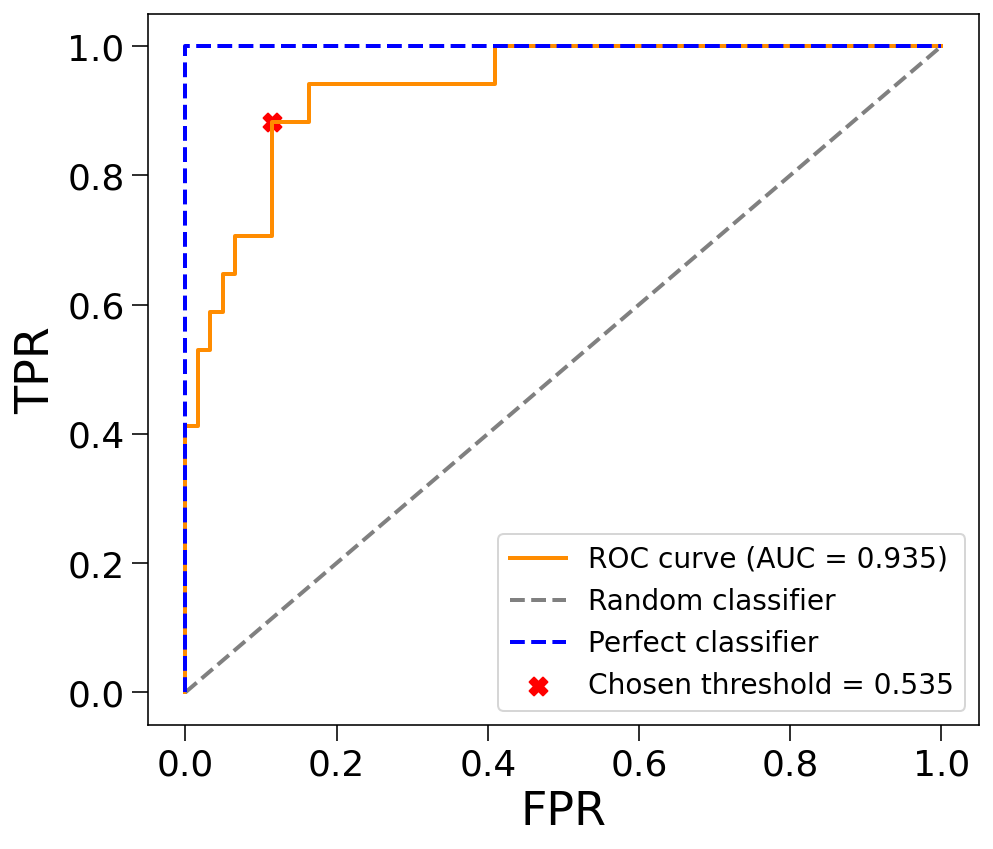
The two classes in our data set are not equally represented, with 61 SDSS spectra of pre-bouncers and 17 SDSS spectra of period-bouncers, corresponding to an approximate ratio of 3:1. To prevent the logistic regression from being biased towards the majority class, we used balanced class weights during training (see e.g. 37). This way, the loss function assigns a higher penalty to misclassifications of the minority class in proportion to the inverse of their class frequency. In consequence, the model becomes more sensitive to the underrepresented class, in our case the period-bouncers, resulting in a more balanced predictive performance across both classes.

To prevent overfitting, L2 regularisation (ridge penalty; 41, 40) was applied during training, with the regularisation strength controlled by the inverse penalty parameter set to $\text{C}=0.4$ .

E.2 Evaluation

Given the limited number of spectra for period-bouncers, we did not reserve a separate test data set for evaluating the performance of the model, instead, we implemented k-fold stratified cross-validation (see e.g. 54). In this method, the sample is split into k disjoint folds of approximately equal size. An untrained copy of the model is trained on k-1 folds and evaluated on the remaining fold, being this process repeated k times so that each object in the sample is used exactly once for testing the model. Stratification divides the data into distinct groups based on their class labels and then randomly selects examples from each group in proportion to their representation in the full data set. Thus, it ensures that the class proportions are preserved in each fold, which is particularly important in our case due to the class imbalance. We used k = 3 folds.

The predictions from each test fold can be summarised in terms of four outcomes: number of true positives (TP), true negatives (TN), false positives (FP), and false negatives (FN) (see Fig. 10 in Sect. 4.1). Based on these quantities, we compute both class-specific and global performance metrics. In each iteration, all evaluation metrics are computed on the test fold and the mean across the iterations is calculated to provide an estimate of the model’s generalisation performance. The variability across folds allows us to quantify an uncertainty for each metric, expressed as the standard deviation. We report in Table 5 the class-specific and global precision, recall, and F1-score (see Eqs. 9–11) (49, 13, 5).

\text{Precision}=\dfrac{\text{TP}}{\text{TP}+\text{FP}},

(9)

\text{Recall}=\dfrac{\text{TP}}{\text{TP}+\text{FN}},

(10)

\text{F1}=\dfrac{2\cdot\text{Precision}\cdot\text{Recall}}{\text{Precision}+\text{Recall}},

(11)

\text{Accuracy}=\dfrac{\text{TP}+\text{TN}}{\text{TP}+\text{TN}+\text{FP}+\text{FN}},

(12)

Precision quantifies the reliability of positive classifications, recall measures the degree of completeness, and the F1-score, defined as the harmonic mean of precision and recall, summarises the trade-off between the two. Global metrics are obtained as the unweighted mean between the class-specific metrics (macro-averaging), thus ensuring that each class contributes equally, regardless of its frequency in the data set. Additionally, we report in Table 5 the accuracy of the model (see Eq. 12), which measures the aggregate rate of correct predictions. We note that the accuracy of the model is defined only globally.

E.3 Final model

The final model coefficients were determined by training on the complete data set, and coefficient uncertainties were quantified using a bootstrap approach. In this procedure, the data set of all Balmer decrement measurements was repeatedly resampled with replacement to generate new pseudo-samples, using stratification to preserve the class proportions in each pseudo-sample. Consequently, some measurements may appear multiple times within a pseudo-sample, while others may not be selected at all. In each iteration, an untrained copy of the model was trained on the resampled data. This process was iterated 1000 times, yielding distributions for each coefficient. The standard deviation of these distributions was adopted as the corresponding uncertainty estimate. The final model coefficients and their uncertainties are $\beta_{0}=-0.953\pm 0.085$ , $\beta_{1}=1.40\pm 0.11$ , and $\beta_{2}=-1.01\pm 0.16$ .

Table 5: Class-specific and global performance metrics of the logistic regression model.

Metric	Pre-bouncers	Period-bouncers	Global
Precision	$0.966\pm 0.024$	$0.701\pm 0.114$	$0.833\pm 0.047$
Recall	$0.887\pm 0.058$	$0.889\pm 0.079$	$0.888\pm 0.016$
F1	$0.923\pm 0.023$	$0.772\pm 0.049$	$0.847\pm 0.036$
Accuracy	-	-	$0.885\pm 0.031$

The decision threshold, that is, the probability value above which a system is classified as a period-bouncer, was chosen to maximize the F1-score of the period-bouncer class, providing an optimal trade-off between precision and recall for period-bouncers. The optimal threshold value is $P_{\text{PB}}=0.535$ , and it was determined using cross-validated out-of-fold predictions, that is, the prediction for each observation was generated by a model trained on the remaining folds during cross-validation, thus ensuring an unbiased estimate of model performance. The same threshold value was consistently applied during the cross-validation evaluation of the model (see Appendix E.2). In Fig. 14, we additionally present the Receiver Operating Characteristic (ROC) curve (107), which illustrates the true positive rate (TPR) against the false positive rate (FPR) across all possible threshold values. As a measure of the model’s discriminative capability, we report the ROC Area Under Curve (AUC) (35), which is $\text{ROC\,AUC}=0.935$ , indicating strong discriminative performance. The ROC curve and ROC AUC metric were calculated using cross-validated out-of-fold predictions. The chosen optimal threshold value at $P_{\text{PB}}=0.535$ is indicated in Fig. 14. As can be seen, the model’s performance lies close to that of a perfect classifier, and the chosen threshold value is also well supported from this perspective.