跳到论文正文
W Papers独立论文阅读器 arXiv:2606.09153 论文正文 计算阅读时间 · 0%
引用这篇论文根据当前论文元数据生成,正式投稿前建议核对。


License: arXiv.org perpetual non-exclusive license
arXiv:2606.09153v1 [math.ST] 08 Jun 2026

The Asymptotic Distribution of Sample Canonical Directions in Gaussian Spiked High-dimensional CCA

Zhangni Pu puzn687@nenu.edu.cn KLASMOE, Key Laboratory of Big Data Analysis of Jilin Province and School of Mathematics & Statistics, Northeast Normal University, No. 5268 People’s Street, Changchun 130024, China Zhangxiao Zhuo zhangxz722@nenu.edu.cn KLASMOE, Key Laboratory of Big Data Analysis of Jilin Province and School of Mathematics & Statistics, Northeast Normal University, No. 5268 People’s Street, Changchun 130024, China Jiang Hu huj156@nenu.edu.cn KLASMOE, Key Laboratory of Big Data Analysis of Jilin Province and School of Mathematics & Statistics, Northeast Normal University, No. 5268 People’s Street, Changchun 130024, China
Abstract

This paper studies the asymptotic behavior of sample canonical directions in a finite-rank spiked high-dimensional canonical correlation analysis model under a Gaussian population assumption. Under the asymptotic regime in which the dimensions of the two data blocks grow proportionally with the sample size, sample canonical directions are generally not consistent estimators of their population counterparts, even when the corresponding sample canonical correlations separate from the bulk spectrum. To quantify directional recovery, we investigate the squared alignment between a sample canonical direction and its associated population direction. For each simple population spike, we first establish a deterministic first-order limit for this squared alignment, which gives an explicit measure of the population-level directional information retained by the sample direction. We then prove a central limit theorem for its fluctuations around the deterministic limit, with an explicit asymptotic variance expressed through deterministic limits of resolvent trace functionals. To make the theoretical quantities computable from data, we further construct plug-in estimators for both the limiting mean and the asymptotic variance by inverting the deterministic outlier eigenvalue map, and prove their consistency. Numerical simulations and a real-data illustration support the theoretical results and demonstrate how the proposed estimators assess the recovery quality of sample canonical directions.

Keywords: Canonical correlation analysis, Random matrix theory, Spiked model, Sample canonical directions, Central limit theorem, Eigenvector alignment

1 Introduction

Canonical correlation analysis (CCA), introduced by Hotelling [14, 13], is a classical method for studying the linear association between two random vectors. Given two centered random vectors 𝐱{\bf x} in ℝp\mathbb{R}^{p} and 𝐲{\bf y} in ℝq\mathbb{R}^{q}, CCA seeks pairs of linear combinations whose correlations are successively maximized. In the population formulation, the squared canonical correlations and the associated canonical directions are determined by the eigenstructure of the population canonical correlation matrix

𝚺x​x−1​𝚺x​y​𝚺y​y−1​𝚺y​x.\boldsymbol{\Sigma}_{xx}^{-1}\boldsymbol{\Sigma}_{xy}\boldsymbol{\Sigma}_{yy}^{-1}\boldsymbol{\Sigma}_{yx}.

In the sample formulation, they are estimated by the eigenvalues and eigenvectors of the sample canonical correlation matrix

𝐒x​x−1​𝐒x​y​𝐒y​y−1​𝐒y​x.{\bf S}_{xx}^{-1}{\bf S}_{xy}{\bf S}_{yy}^{-1}{\bf S}_{yx}.

This eigenvalue-eigenvector representation makes CCA particularly suitable for analysis through random matrix theory.

Classical multivariate analysis studies CCA in the regime where pp and qq are fixed while n→∞n\to\infty; see, for example, [21, 1]. In many modern applications, however, the dimensions of the two data blocks are comparable to the sample size. In such high-dimensional regimes, sample canonical correlations and their associated directions exhibit behavior that is fundamentally different from classical low-dimensional asymptotics. In particular, sample canonical directions need not consistently estimate their population counterparts, even when the associated signal eigenvalues are separated from the noise bulk.

Let the columns of (𝐗⊤,𝐘⊤)⊤({\bf X}^{\top},{\bf Y}^{\top})^{\top} be nn independent observations of the centered random vector (𝐱⊤,𝐲⊤)⊤({\bf x}^{\top},{\bf y}^{\top})^{\top}. Denote the population covariance matrix by

𝚺=(𝚺x​x𝚺x​y𝚺y​x𝚺y​y).\displaystyle\boldsymbol{\Sigma}=\begin{pmatrix}\boldsymbol{\Sigma}_{xx}&\boldsymbol{\Sigma}_{xy}\\ \boldsymbol{\Sigma}_{yx}&\boldsymbol{\Sigma}_{yy}\end{pmatrix}.

The population squared canonical correlations rir_{i} and the corresponding population canonical directions 𝒖i{\boldsymbol{u}}_{i} are determined by

𝚺x​x−1​𝚺x​y​𝚺y​y−1​𝚺y​x​𝒖i=ri​𝒖i.\boldsymbol{\Sigma}_{xx}^{-1}\boldsymbol{\Sigma}_{xy}\boldsymbol{\Sigma}_{yy}^{-1}\boldsymbol{\Sigma}_{yx}{\boldsymbol{u}}_{i}=r_{i}{\boldsymbol{u}}_{i}.

The sample analogues are the eigenvalues lil_{i} and eigenvectors 𝝂i\boldsymbol{\nu}_{i} of

𝐒x​x−1​𝐒x​y​𝐒y​y−1​𝐒y​x.{\bf S}_{xx}^{-1}{\bf S}_{xy}{\bf S}_{yy}^{-1}{\bf S}_{yx}.

The main objective of this paper is to quantify, in a finite-rank spiked high-dimensional CCA model, how well a sample canonical direction 𝝂i\boldsymbol{\nu}_{i} aligns with its population counterpart 𝒖i{\boldsymbol{u}}_{i}.

Throughout the theoretical analysis we work in the Gaussian spiked CCA model

𝐗=𝚲​𝐘+𝚪​𝐖,𝚲​𝚲⊤+𝚪​𝚪⊤=𝐈p,{\bf X}=\boldsymbol{\Lambda}{\bf Y}+\boldsymbol{\Gamma}{\bf W},~~\boldsymbol{\Lambda}\boldsymbol{\Lambda}^{\top}+\boldsymbol{\Gamma}\boldsymbol{\Gamma}^{\top}={\bf I}_{p},

following the spiked CCA framework in [8]. Here 𝐘{\bf Y} and 𝐖{\bf W} have independent Gaussian entries. The nonzero eigenvalues of 𝚲​𝚲⊤\boldsymbol{\Lambda}\boldsymbol{\Lambda}^{\top} are the population spikes r1,…,rkr_{1},\dots,r_{k}. Since canonical directions are defined only up to sign, we measure directional recovery through the squared alignment

⟨𝒖i,𝝂i⟩2.\langle{\boldsymbol{u}}_{i},\boldsymbol{\nu}_{i}\rangle^{2}.

This quantity is the squared cosine of the angle between the population and sample canonical directions and is invariant under sign changes of the eigenvectors.

We work under the following dimensional assumption.

Assumption 1.1 (On the dimensions).

We assume that p:=p​(n)p:=p(n), q:=q​(n)q:=q(n), and, as n→∞n\to\infty,

p/n→c1∈(0,1),q/n→c2∈(0,1), s.t. ​c1+c2∈(0,1).p/n\to c_{1}\in(0,1),~~~~q/n\to c_{2}\in(0,1),~~~~\mbox{ s.t. \par\par}c_{1}+c_{2}\in(0,1).

Without loss of generality, we always work with the additional assumption p>qp>q, thus c1>c2c_{1}>c_{2}.

Assumption 1.2 (On the population spiked model).

We assume that rank​(𝚺x​y)=k\text{rank}(\boldsymbol{\Sigma}_{xy})=k for some fixed positive integer kk. Let rir_{i} denote the ii-th largest non-zero eigenvalue of the population matrix 𝚺x​x−1​𝚺x​y​𝚺y​y−1​𝚺y​x\boldsymbol{\Sigma}_{xx}^{-1}\boldsymbol{\Sigma}_{xy}\boldsymbol{\Sigma}_{yy}^{-1}\boldsymbol{\Sigma}_{yx}. We assume these eigenvalues are ”spiked”:

1>r1≥⋯≥ri≥⋯≥rk>rc:=c1​c2(1−c1)​(1−c2).1>r_{1}\geq\dots\geq r_{i}\geq\dots\geq r_{k}>r_{c}:=\sqrt{\frac{c_{1}c_{2}}{(1-c_{1})(1-c_{2})}}.
Remark 1.3.

The threshold rcr_{c} is the phase-transition threshold for sample canonical correlation matrices [8, 20]. Population spikes above this threshold produce sample eigenvalues that separate from the upper edge of the bulk limiting spectral distribution. Under Assumption 1.2, the associated sample eigenvalues are therefore sample spiked eigenvalues, and the corresponding sample eigenvectors can be studied individually.

1.1 Previous related theoretical results

We first recall the spectral theory for sample canonical correlation matrices in the high-dimensional null and spiked settings. The empirical spectral distribution (ESD)

Fn​(x):=1q​∑i=1qI​(li≤x)F_{n}(x):=\frac{1}{q}\sum_{i=1}^{q}I(l_{i}\leq x)

converges weakly to a deterministic probability distribution F​(x)F(x) [24], whose density is

f​(x)=12​π​c2​(d+−x)​(x−d−)x​(1−x)​I​(d−≤x≤d+),\displaystyle f(x)=\frac{1}{2\pi c_{2}}\frac{\sqrt{(d_{+}-x)(x-d_{-})}}{x(1-x)}I(d_{-}\leq x\leq d_{+}), (1)

where d±=(c1​(1−c2)±c2​(1−c1))2d_{\pm}=(\sqrt{c_{1}(1-c_{2})}\pm\sqrt{c_{2}(1-c_{1})})^{2}. Central limit theorems for linear spectral statistics and related global spectral quantities have been further developed in [28, 29, 30].

In the finite-rank setting, the sample canonical correlation matrix 𝐒x​x−1​𝐒x​y​𝐒y​y−1​𝐒y​x{\bf S}_{xx}^{-1}{\bf S}_{xy}{\bf S}_{yy}^{-1}{\bf S}_{yx} can be viewed as a finite-rank perturbation of the null model. The perturbation does not change the limiting spectral distribution of the bulk, but sufficiently strong population canonical correlations generate sample outliers. Bao et al. [8] analyzed the limiting behavior and fluctuations of its largest eigenvalues in this spiked setting. Let

γi:=ri​(1−c1+c1​ri−1)​(1−c2+c2​ri−1).\displaystyle\gamma_{i}:=r_{i}(1-c_{1}+c_{1}r_{i}^{-1})(1-c_{2}+c_{2}r_{i}^{-1}). (2)
Theorem 1.4 (Theorem 1.7 of [8]).

Under Assumptions 1.1 and 1.2, the squares of the sample canonical coefficients exhibit the following convergence:

  1. 1.

    (Outliers) For 1≤i≤k1\leq i\leq k, as n→∞n\to\infty, we have li−γi→a.s.0l_{i}-\gamma_{i}\xrightarrow{a.s.}0.

  2. 2.

    (Sticking eigenvalues) For each fixed i≥k+1i\geq k+1, as n→∞n\to\infty, we have li−d+→a.s.0l_{i}-d_{+}\xrightarrow{a.s.}0.

Extensions of the spiked CCA eigenvalue theory to non-Gaussian populations and related Fisher-type models have been studied in [20, 27, 4, 15]. These eigenvalue results provide the spectral foundation for signal detection in high-dimensional CCA. However, eigenvalue separation alone does not quantify directional recovery. A separated sample canonical correlation indicates that a signal is detectable from the spectrum, but it does not describe how accurately the associated sample canonical direction estimates the corresponding population direction. This distinction motivates the eigenvector analysis developed in this paper.

The study of eigenvectors in random matrix theory (RMT) is generally more challenging than that of eigenvalues. Global-level results have investigated eigenvector empirical spectral distributions (VESD) and related quantities [3, 26, 25, 17]. Local-level studies, which are close to the goal of this paper, characterize the ”distance” or ”alignment” between an individual sample eigenvector and a fixed population direction. Such phenomena have been studied for spiked sample covariance matrices [22, 6, 23], deformed Wigner matrices [11, 16, 9], and information-plus-noise models [7, 18]. These works show that the squared inner product between a sample eigenvector and its population counterpart is a natural measure of directional recovery.

For high-dimensional CCA, the eigenvector problem remains less developed. Bykhovskaya and Gorin [10] study the high-dimensional behavior of canonical variables, or canonical variates, and obtain first-order limits for angles between sample and population canonical variables such as 𝐗⊤​𝝂i{\bf X}^{\top}\boldsymbol{\nu}_{i}, 𝐗⊤​𝒖i{\bf X}^{\top}{\boldsymbol{u}}_{i}. These angles are defined in the sample space. They are different from the alignment between the canonical direction vectors themselves, namely the eigenvectors and their population counterparts in the original variable spaces. The latter quantity is sensitive to the covariance structure and coordinate normalization. In particular, an asymptotic theory for the squared alignment ⟨𝒖i,𝝂i⟩2\langle{\boldsymbol{u}}_{i},\boldsymbol{\nu}_{i}\rangle^{2} in a finite-rank spiked CCA model does not seem to be available in the existing literature.

1.2 Contributions and Overview of Results

This paper develops a first- and second-order asymptotic theory for sample canonical directions associated with finite-rank population spikes in high-dimensional CCA under Gaussian assumptions. Our object of interest is the squared alignment

⟨𝒖i,𝝂i⟩2,\langle{\boldsymbol{u}}_{i},\boldsymbol{\nu}_{i}\rangle^{2},

which measures the amount of population-level directional information retained by the sample canonical direction.

Our first contribution is a deterministic first-order characterization of this squared alignment. For each simple spike rir_{i}, we prove that

⟨𝒖i,𝝂i⟩2→𝑝11+d​(ri),\langle{\boldsymbol{u}}_{i},\boldsymbol{\nu}_{i}\rangle^{2}\xrightarrow{p}\frac{1}{1+d(r_{i})},

where d​(ri)d(r_{i}) is an explicit function of the population spike rir_{i} and c1,c2c_{1},c_{2}. The limit is generally strictly smaller than one. Thus, the sample canonical direction is not classically consistent in the high-dimensional regime. At the same time, the result gives an explicit limiting measure of the recovery quality of the sample direction. Similar non-consistency phenomena and nontrivial eigenvector alignment limits have appeared in other spiked random matrix models, including spiked sample covariance matrices [22, 6, 23], deformed Wigner matrices [11], and information-plus-noise matrices [7, 18].

Our main contribution is a CLT for the fluctuation of the squared alignment. Specifically, we show that

n​(⟨𝒖i,𝝂i⟩2−11+d​(ri))\sqrt{n}\left(\langle{\boldsymbol{u}}_{i},\boldsymbol{\nu}_{i}\rangle^{2}-\frac{1}{1+d(r_{i})}\right)

converges in distribution to a centered normal distribution with variance σ2​(ri)/(1+d​(ri))4\sigma^{2}(r_{i})/(1+d(r_{i}))^{4}. Here σ​(ri)2\sigma(r_{i})^{2} is given explicitly in terms of deterministic limits of resolvent trace functionals. To the best of our knowledge, this is the first CLT for the squared alignment between a sample canonical direction and its population counterpart in the finite-rank spiked high-dimensional CCA model. This result upgrades the directional recovery theory from a deterministic approximation to a distributional approximation.

Our third contribution is to make the preceding asymptotic quantities estimable from data. Since both the limiting mean and the asymptotic variance depend on the unknown population spike rir_{i}, we estimate rir_{i} through the deterministic outlier map

r^i=γ−1​(li).\hat{r}_{i}=\gamma^{-1}(l_{i}).

Substituting r^i\hat{r}_{i} into the deterministic expressions yields plug-in estimators

μ^i=11+d​(r^i)a​n​dτ^i2=σ2​(r^i)(1+d​(r^i))4.\hat{\mu}_{i}=\dfrac{1}{1+d(\hat{r}_{i})}~~~~and~~~~\hat{\tau}_{i}^{2}=\dfrac{\sigma^{2}(\hat{r}_{i})}{(1+d(\hat{r}_{i}))^{4}}.

We prove that these estimators consistently estimate the limiting mean and asymptotic variance of the squared alignment, respectively. Consequently, the theory provides a sample-based measure of both the strength and the uncertainty of directional recovery.

On the technical side, our proof is based on a detailed analysis of the characteristic equation for the sample canonical correlation matrix. By applying the Schur complement, the eigenvector problem is reduced to the study of a finite-dimensional random matrix involving resolvents of the noise part of the CCA matrix. This reduction expresses the normalization of the sample eigenvector in terms of finite-dimensional random matrices involving resolvents of the noise part of the model. We then derive deterministic equivalents and fluctuation estimates for the resulting resolvent trace functionals. The Gaussian assumption allows us to use the Gaussian Poincaré inequality and Stein’s lemma, or equivalently the Gaussian cumulant expansion, to control variances and compute the limiting covariance structure.

Finally, we provide numerical illustrations to support the theoretical results. The simulation study illustrates the first-order deterministic limit and the Gaussian fluctuation in rank-one and multi-spike settings. We also present a real-data illustration using the limestone grassland community data originally reported by Gittins [12] and also analyzed in Bao et al. [8]. In this example, the leading sample squared canonical correlation separates from the bulk, and the plug-in estimate μ^1\hat{\mu}_{1} provides a quantitative assessment of the recovery quality of the leading sample canonical direction. This illustrates how the proposed theory can be used to interpret sample canonical directions when the corresponding population directions are unobservable.

1.3 Organization and notation

The remainder of the paper is organized as follows. Section 2 presents the preliminary technical lemmas and our main theoretical results, including the first-order limit and the central limit theorem for the squared alignment. Section 3 constructs plug-in estimators for the limiting mean and asymptotic variance of the squared alignment and presents a real-data illustration. Section 4 reports Monte Carlo simulations supporting the theoretical results. Section 5 proves the main theorems, while the remaining sections provide the required technical estimates.

Throughout the paper, ||⋅||||\cdot|| denotes the Euclidean norm for vectors and the operator norm for matrices. For a matrix 𝐀{\bf A}, tr​𝐀{\rm tr}{\bf A} denotes its trace, and 𝐀⊤{\bf A}^{\top} denotes its transpose. We write →𝑝\xrightarrow{p}, →a.s.\xrightarrow{a.s.}, and →𝐷\xrightarrow{D} for convergence in probability, almost sure convergence, and convergence in distribution, respectively.

2 Main Results

In this section, we state our main results and introduce the necessary technical lemmas that support our proofs and calculations in the subsequent sections.

2.1 Preliminary Technical Lemmas

We begin with several standard definitions and results that are fundamental to our analysis.

Definition 2.1.

Let ξn{\xi_{n}} be a sequence of random variables and {Cn}\{C_{n}\} be a sequence of positive constants. We say ξn=Op​(Cn)\xi_{n}=O_{p}(C_{n}) if for all ε>0\varepsilon>0, there exist constants NεN_{\varepsilon} and KεK_{\varepsilon} such that for all n>Nεn>N_{\varepsilon}, ℙ​(|ξn/Cn|≤Kε)≥1−ε\mathbb{P}(|\xi_{n}/C_{n}|\leq K_{\varepsilon})\geq 1-\varepsilon.

Note that if supn𝔼​|ξn|l<∞\sup_{n}\mathbb{E}|\xi_{n}|^{l}<\infty for some l≥1l\geq 1, then ξn=Op​(1)\xi_{n}=O_{p}(1) by Markov’s inequality. The following cumulant expansion formula plays a central role in our computation, with a proof found in [19].

Lemma 2.2 (Cumulant expansion formula).

Let f:ℝ→ℂf:\mathbb{R}\to\mathbb{C} be a smooth function, and denote by f(k)f^{(k)} its kkth derivative. Then for every fixed l∈ℕl\in\mathbb{N}, we have

𝔼​[ξ​f​(ξ)]=∑k=0lκk+1​(ξ)k!​𝔼​[f(k)​(ξ)]+ℛl+1,\displaystyle\mathbb{E}[\xi f(\xi)]=\sum_{k=0}^{l}\frac{\kappa_{k+1}(\xi)}{k!}\mathbb{E}[f^{(k)}(\xi)]+\mathcal{R}_{l+1}, (3)

assuming that all expectations in (3) exist, where ℛl+1\mathcal{R}_{l+1} is the remainder term (depending on ff and ξ\xi), such that for any t>0t>0,

ℛl+1=O​(1)​𝔼​[|ξ|l+2​I​|ξ|>t]​supx∈ℝ|f(l+1)​(x)|+O​(1)​𝔼​[|ξ|l+2]​sup|x|≤t|f(l+1)​(x)|.\displaystyle\mathcal{R}_{l+1}=O(1)\mathbb{E}[|\xi|^{l+2}I{|\xi|>t}]\sup_{x\in\mathbb{R}}|f^{(l+1)}(x)|+O(1)\mathbb{E}[|\xi|^{l+2}]\sup_{|x|\leq t}|f^{(l+1)}(x)|.

In particular, if ξ\xi is from a standard normal distribution, κ1​(ξ)=0,κ2​(ξ)=1\kappa_{1}(\xi)=0,\kappa_{2}(\xi)=1, and κj​(ξ)=0\kappa_{j}(\xi)=0 for j≥3j\geq 3. We then get the famous Stein’s Lemma:

𝔼​[ξ​f​(ξ)]=𝔼​[f′​(ξ)].\displaystyle\mathbb{E}[\xi f(\xi)]=\mathbb{E}[f^{\prime}(\xi)]. (4)
Lemma 2.3 (Gaussian Poincaré inequality).

Let μ\mu be the standard Gaussian measure on M=ℝnM=\mathbb{R}^{n}. Assume f:ℝn→ℝf:\mathbb{R}^{n}\to\mathbb{R} is C1C^{1}. Then, Varμ⁡(f)≤C​𝔼μ​|∇f|2\operatorname{Var}_{\mu}(f)\leq C\mathbb{E}_{\mu}|\nabla f|^{2} holds with C=1C=1. In particular, let {ξi}i=1n\{\xi_{i}\}_{i=1}^{n} with standard normal distribution be independent, and assume the function f:ℝn→ℝf:\mathbb{R}^{n}\to\mathbb{R} has first-order continuous partial derivatives. Then we have

Var⁡[f​(ξ1,…,ξn)]≤𝔼​∑i=1n[∂f​(ξ1,…,ξn)∂ξi]2.\displaystyle\operatorname{Var}[f(\xi_{1},\dots,\xi_{n})]\leq\mathbb{E}\sum_{i=1}^{n}\left[\frac{\partial f(\xi_{1},\dots,\xi_{n})}{\partial\xi_{i}}\right]^{2}.

2.2 Asymptotic Results for the Squared Alignment

Under the model 𝐗=𝚲​𝐘+𝚪​𝐖{\bf X}=\boldsymbol{\Lambda}{\bf Y}+\boldsymbol{\Gamma}{\bf W}, the finite-rank population correlation structure is encoded in 𝚲\boldsymbol{\Lambda}. Since the population and sample canonical directions are defined only up to sign and are normalized to have unit norm, we study the squared inner product between them. The squared inner product ⟨𝒖i,𝝂i⟩2\langle{\boldsymbol{u}}_{i},\boldsymbol{\nu}_{i}\rangle^{2} is the squared cosine of the angle between the population and sample canonical directions. The first-order approximation of the squared cosine of this angle is given below.

Theorem 2.4 (First-order limit).

Under Assumptions 1.1-1.2, fix 1≤i≤k1\leq i\leq k such that rir_{i} is a simple spike. Then

⟨𝒖i,𝝂i⟩2→𝑝11+d​(ri),\displaystyle\langle{\boldsymbol{u}}_{i},\boldsymbol{\nu}_{i}\rangle^{2}\xrightarrow{p}\frac{1}{1+d(r_{i})}, (5)

where d​(ri)=D1​(ri)+D2​(ri),d(r_{i})=D_{1}(r_{i})+D_{2}(r_{i}), and

D1​(ri)=\displaystyle D_{1}(r_{i})= (1−ri)(2​(η​ri−ω)​(1−ri)−ririF1(ri)\displaystyle(1-r_{i})\left(\frac{2(\eta r_{i}-\omega)(1-r_{i})-r_{i}}{r_{i}}F_{1}(r_{i})\right.
+ri​(η​ri−ω)​(1−ri)−(η​ri−ω)2​(1−ri)2ri2F2(ri)),\displaystyle\left.+\frac{r_{i}(\eta r_{i}-\omega)(1-r_{i})-(\eta r_{i}-\omega)^{2}(1-r_{i})^{2}}{r_{i}^{2}}F_{2}(r_{i})\right),
D2​(ri)=\displaystyle D_{2}(r_{i})= ri​(η​ri−ω)2​(1−ri)2c2​ri2((c1​ri+ω​(1−ri)ri−(η​ri−ω)​(1−ri)−ωη​ri−ω)F1(ri)\displaystyle\frac{r_{i}(\eta r_{i}-\omega)^{2}(1-r_{i})^{2}}{c_{2}r_{i}^{2}}\left(\left(\frac{c_{1}r_{i}+\omega(1-r_{i})}{r_{i}-(\eta r_{i}-\omega)(1-r_{i})}-\frac{\omega}{\eta r_{i}-\omega}\right)F_{1}(r_{i})\right.
+(c1+c2−2​ω​(1−ri)ri)F2(ri)),\displaystyle\left.+\left(c_{1}+c_{2}-\frac{2\omega(1-r_{i})}{r_{i}}\right)F_{2}(r_{i})\right),
F1​(ri)=\displaystyle F_{1}(r_{i})= −c1​ri​((1−c2)​ri+c2)ri​(η​ri−ω)−(η​ri−ω)2​(1−ri),\displaystyle\frac{-c_{1}r_{i}((1-c_{2})r_{i}+c_{2})}{r_{i}(\eta r_{i}-\omega)-(\eta r_{i}-\omega)^{2}(1-r_{i})},
F2​(ri)=\displaystyle F_{2}(r_{i})= ri2​(ω​(1−c2)​ri​((1−c1)​ri+c1)+c1​(η​ri−ω)​(η​ri2−ω))((1−c1)​ri+c1)2​((1−c2)​ri+c2)​(η​ri−ω)2​(η​ri2−ω),\displaystyle\frac{r_{i}^{2}\left(\omega(1-c_{2})r_{i}\big((1-c_{1})r_{i}+c_{1}\big)+c_{1}(\eta r_{i}-\omega)(\eta r_{i}^{2}-\omega)\right)}{\big((1-c_{1})r_{i}+c_{1}\big)^{2}\big((1-c_{2})r_{i}+c_{2}\big)(\eta r_{i}-\omega)^{2}(\eta r_{i}^{2}-\omega)},

with η=(1−c1)​(1−c2)\eta=(1-c_{1})(1-c_{2}) and ω=c1​c2\omega=c_{1}c_{2}.

Theorem 2.4 shows that the squared inner product has a deterministic limit, which implies that the sample spiked eigenvector 𝝂i\boldsymbol{\nu}_{i} is asymptotically inconsistent, lying on a cone around the true population spiked eigenvector 𝒖i{\boldsymbol{u}}_{i}. Similar behavior has been observed in several spiked random matrix models, including spiked sample covariance matrices [22, 6, 23], deformed Wigner matrices [11], and information-plus-noise matrices [7, 18]. We next study the fluctuations of the squared alignment around this first-order limit. This leads to the following central limit theorem.

Theorem 2.5 (Central limit theorem).

Under the same assumptions as in Theorem 2.4, for the same simple spike rir_{i}, the following convergence in distribution holds:

n​(⟨𝒖i,𝝂i⟩2−11+d​(ri))→𝐷𝒩​(0,σ2​(ri)/(1+d​(ri))4),\displaystyle\sqrt{n}\left(\langle{\boldsymbol{u}}_{i},\boldsymbol{\nu}_{i}\rangle^{2}-\frac{1}{1+d(r_{i})}\right)\xrightarrow{D}\mathcal{N}(0,\sigma^{2}(r_{i})/(1+d(r_{i}))^{4}), (6)

where

σ2​(ri)=\displaystyle\sigma^{2}(r_{i})= 2​(1−ri)2​P1​(ri)−4​η​ri−ωri​(1−ri)3​(P1​(ri)+F3​(ri))\displaystyle 2(1-r_{i})^{2}P_{1}(r_{i})-4\frac{\eta r_{i}-\omega}{r_{i}}(1-r_{i})^{3}(P_{1}(r_{i})+F_{3}(r_{i})) (7)
+2​(η​ri−ω)2ri2​(1−ri)4​(P1​(ri)+2​F3​(ri)+Q3​(ri))\displaystyle+\frac{2(\eta r_{i}-\omega)^{2}}{r_{i}^{2}}(1-r_{i})^{4}(P_{1}(r_{i})+2F_{3}(r_{i})+Q_{3}(r_{i}))
+2​(η​ri−ω)4​(1−ri)4ri2​(Jk​1​(ri)+Jk​2​(ri)+Jk​3​(ri)+Jk​4​(ri)+Jk​5​(ri))\displaystyle+\frac{2(\eta r_{i}-\omega)^{4}(1-r_{i})^{4}}{r_{i}^{2}}\left(J_{k1}(r_{i})+J_{k2}(r_{i})+J_{k3}(r_{i})+J_{k4}(r_{i})+J_{k5}(r_{i})\right)
+4​(η​ri−ω)3​(1−ri)4​Q4​(ri)c2​ri2+4​c1​(η​ri−ω)2​(1−ri)3​Q7​(ri)c2​ri.\displaystyle+\frac{4(\eta r_{i}-\omega)^{3}(1-r_{i})^{4}Q_{4}(r_{i})}{c_{2}r_{i}^{2}}+\frac{4c_{1}(\eta r_{i}-\omega)^{2}(1-r_{i})^{3}Q_{7}(r_{i})}{c_{2}r_{i}}. (8)

The deterministic quantities P1​(ri)P_{1}(r_{i}), F3​(ri)F_{3}(r_{i}), Q3​(ri)Q_{3}(r_{i}), Jk​ℓ​(ri)J_{k\ell}(r_{i}), ℓ=1,…,5\ell=1,\ldots,5, Q4​(ri)Q_{4}(r_{i}), and Q7​(ri)Q_{7}(r_{i}) are defined in (24), (36), (37), (31) – (35), (38), and (40), respectively.

Remark 2.6.

To the best of our knowledge, Theorem 2.5 is the first central limit theorem for the squared alignment ⟨𝒖i,𝝂i⟩2\langle{\boldsymbol{u}}_{i},\boldsymbol{\nu}_{i}\rangle^{2} in high-dimensional CCA with finite-rank population spikes. This result is proved under Assumptions 1.1–1.2, for a fixed number of spikes and for a simple spike in the separated, supercritical regime. Critical or near-critical spikes, multiple spikes with the same limiting location, and possible interactions among several spikes are not considered here.

3 Estimation of the Asymptotic Mean and Variance of the Squared Alignment

In the previous section, we show that, for each simple spike rir_{i}, the squared alignment

⟨𝒖i,𝝂i⟩2\langle{\boldsymbol{u}}_{i},\boldsymbol{\nu}_{i}\rangle^{2}

does not converge to one. Instead, it converges to a nontrivial limit that is strictly smaller than one. Moreover, the fluctuation around this limit occurs on the n−1/2n^{-1/2} scale and admits an asymptotically Gaussian description. Thus, under the high-dimensional regime considered in this paper, the sample canonical direction is not a classically consistent estimator of the population canonical direction. Instead, its squared alignment with the population direction has a nontrivial limiting value.

This suggests that, in the present setting, the relevant question is not whether the sample canonical direction fully recovers the population one, but how large the limiting squared alignment is and how it fluctuates around its limit. Theorem 2.4 identifies the asymptotic center of this alignment, while Theorem 2.5 characterizes its second-order fluctuation. However, both quantities depend on the population spike rir_{i}, and are therefore not directly computable from data. The purpose of this section is to construct plug-in estimators for these quantities based on the sample spiked eigenvalue lil_{i}, thereby turning the asymptotic results of Theorems 2.4 and 2.5 into quantities that can be evaluated from the observed sample. In this sense, eigenvalue separation and directional recovery represent two different aspects of the problem. A sample spiked eigenvalue indicates that a signal direction is detectable from the spectrum, whereas the squared alignment quantifies how accurately the associated sample direction represents its population counterpart. The estimators constructed below are designed to assess this directional recovery.

3.1 Estimation of the Asymptotic Mean

By Theorem 1.4, for each sample spiked eigenvalue associated with a population spike rir_{i}, we have

li−γi→a.s.0,γi=γ​(ri),l_{i}-\gamma_{i}\xrightarrow{a.s.}0,~~\gamma_{i}=\gamma(r_{i}),

where γ​(⋅)\gamma(\cdot) is the deterministic mapping from the population spike rir_{i} to its associated outlier location. On the other hand, Theorem 2.4 shows that

⟨𝒖i,𝝂i⟩2→𝑝μi,μi:=11+d​(ri).\langle{\boldsymbol{u}}_{i},\boldsymbol{\nu}_{i}\rangle^{2}\xrightarrow{p}\mu_{i},~~\mu_{i}:=\frac{1}{1+d(r_{i})}.

Accordingly, μi\mu_{i} describes the limiting mean of the squared alignment between the sample and population canonical directions. Since μi\mu_{i} depends on the unknown spike rir_{i}, a natural strategy is to estimate rir_{i} from the observed spiked eigenvalue lil_{i}, and then substitute the resulting estimator into the expression for μi\mu_{i}.

Proposition 3.1.

Suppose the assumptions of Theorem 1.4 and 2.4 hold, and fix a simple spike rir_{i}. Assume that the function γ​(⋅)\gamma(\cdot) is locally one-to-one in a neighborhood of rir_{i}, and that d​(⋅)d(\cdot) is continuous at rir_{i}. Denote by γ−1​(⋅)\gamma^{-1}(\cdot) the corresponding local inverse on a neighborhood of γ​(ri)\gamma(r_{i}). Define

r^i:=γ−1​(li),μ^i:=11+d​(r^i).\hat{r}_{i}:=\gamma^{-1}(l_{i}),~~\hat{\mu}_{i}:=\dfrac{1}{1+d(\hat{r}_{i})}.

Then

r^i→𝑝ri,μ^i→𝑝μi.\hat{r}_{i}\xrightarrow{p}r_{i},~~\hat{\mu}_{i}\xrightarrow{p}\mu_{i}.

The proof is postponed to Section 8.

The construction in Proposition 3.1 can be summarized as the following plug-in procedure.

Remark 3.2.

The role of Proposition 3.1 is not to estimate the population direction 𝒖i{\boldsymbol{u}}_{i} itself, but to estimate the limiting mean μi\mu_{i} appearing in Theorem 2.4. Since μi\mu_{i} is precisely the limit of the squared alignment ⟨𝒖i,𝝂i⟩2\langle{\boldsymbol{u}}_{i},\boldsymbol{\nu}_{i}\rangle^{2}, it may be interpreted as the limiting mean of the squared alignment between the sample and population directions. Proposition 3.1 shows that this quantity can be consistently estimated from the observed sample spiked eigenvalue. Thus, μ^i\hat{\mu}_{i} provides a sample-based measure of recovery quality for a direction that is itself not consistently estimable.

Table 1: Plug-in procedure for estimating the limiting mean μi\mu_{i}.
Step Procedure
1 Given the centered data matrices 𝐗∈ℝp×n{\bf X}\in\mathbb{R}^{p\times n} and 𝐘∈ℝq×n{\bf Y}\in\mathbb{R}^{q\times n}, form the sample canonical correlation matrix S_xx^-1S_xyS_yy^-1S_yx. Compute its nonzero eigenvalues l1≥l2≥⋯≥lql_{1}\geq l_{2}\geq\cdots\geq l_{q}.
2 Identify the sample spiked eigenvalues. In practice, retain those lil_{i} satisfying l_i¿d_+, or, more conservatively, li>d++εnl_{i}>d_{+}+\varepsilon_{n}, where εn↓0\varepsilon_{n}\downarrow 0 is a deterministic sequence chosen to separate sample outliers from the bulk edge.
3 For each retained sample spiked eigenvalue lil_{i}, estimate the corresponding population spike by ^r_i=γ^-1(l_i)=2c1c2-c1-c2+li+(li-d-)(li-d+)2(c1c2-c1-c2+1).
4 Compute the plug-in estimator of the limiting mean of the squared alignment: ^μ_i=11+d(^ri).

3.2 Estimation of the Asymptotic Variance

The limiting mean alone does not fully describe the behavior of the squared alignment. Theorem 2.5 further shows that

n​(⟨𝒖i,𝝂i⟩2−11+d​(ri))→𝐷𝒩​(0,σ2​(ri)/(1+d​(ri))4).\sqrt{n}\left(\langle{\boldsymbol{u}}_{i},\boldsymbol{\nu}_{i}\rangle^{2}-\frac{1}{1+d(r_{i})}\right)\xrightarrow{D}\mathcal{N}(0,\sigma^{2}(r_{i})/(1+d(r_{i}))^{4}).

Thus the corresponding asymptotic variance is

τi2:=σ2​(ri)(1+d​(ri))4.\tau_{i}^{2}:=\dfrac{\sigma^{2}(r_{i})}{(1+d(r_{i}))^{4}}.

This quantity measures the fluctuation scale of the squared alignment around its limiting mean. As in the previous subsection, we estimate τi2\tau_{i}^{2} by substituting r^i\hat{r}_{i} into the deterministic expression above.

Proposition 3.3.

Under the assumptions of Proposition 3.1, further assume that σ2​(⋅)\sigma^{2}(\cdot) is continuous at rir_{i}, and that 0<σ2​(ri)<∞0<\sigma^{2}(r_{i})<\infty. Define

τ^i2:=σ2​(r^i)(1+d​(r^i))4,τ^i:=τ^i2,\hat{\tau}_{i}^{2}:=\dfrac{\sigma^{2}(\hat{r}_{i})}{(1+d(\hat{r}_{i}))^{4}},~~\hat{\tau}_{i}:=\sqrt{\hat{\tau}_{i}^{2}},

on the event where τ^i2≥0\hat{\tau}_{i}^{2}\geq 0. Then

τ^i2→𝑝τi2,τ^i→𝑝τi.\hat{\tau}_{i}^{2}\xrightarrow{p}\tau_{i}^{2},~~\hat{\tau}_{i}\xrightarrow{p}\tau_{i}.

The proof is postponed to Section 8.

Remark 3.4.

Proposition 3.3 shows that the asymptotic variance appearing in Theorem 2.5 is likewise estimable from the sample. Consequently, one can estimate not only the limiting mean of the squared alignment itself, but also the scale of its random fluctuation. In this sense, Propositions 3.1 and 3.3 provide complementary information: μ^i\hat{\mu}_{i} estimates the limiting mean of the squared alignment, whereas τ^i\hat{\tau}_{i} estimates its fluctuation scale.

3.3 A Real-Data Illustration

Since the population canonical directions are unobservable in real data, the quantity

⟨𝒖i,𝝂i⟩2\langle{\boldsymbol{u}}_{i},\boldsymbol{\nu}_{i}\rangle^{2}

cannot be evaluated directly. Accordingly, the purpose of this subsection is not to validate the population-level limit in Theorem 2.4, but rather to illustrate how the plug-in estimator proposed in Proposition 3.1 can be used to assess the quality of the leading sample canonical directions in practice. The real-data illustration focuses on the first-order estimator μ^i\hat{\mu}_{i}, since the main purpose is to assess the recovery quality of the detected sample direction.

We consider the limestone grassland community data originally reported in Table A-2 of Gittins [12]. The data contain n=45n=45 sampling sites from a limestone grassland community in Anglesey, North Wales, and include two blocks of variables: an 8-dimensional block of plant species abundances and a 6-dimensional block of soil characteristics. The same dataset was also used in Bao et al. [8] as a real-data example for high-dimensional canonical correlation analysis. Following the standard CCA preprocessing used there, we first center all variables across samples and then form the sample canonical correlation matrix from the centered data.

Let 𝐗{\bf X} and 𝐘{\bf Y} denote the centered species and soil data matrices, with dimensions p×np\times n and q×nq\times n, respectively. We then form the sample canonical correlation matrix

𝐒x​x−1​𝐒x​y​𝐒y​y−1​𝐒y​x,{\bf S}_{xx}^{-1}{\bf S}_{xy}{\bf S}_{yy}^{-1}{\bf S}_{yx},

and compute its leading eigenvalues lil_{i}. The six sample squared canonical correlations computed from the centered Table A-2 data of Gittins [12] are

l1=0.8293,l2=0.5198,l3=0.3589,l4=0.1074,l5=0.0938,l6=0.0378.l_{1}=0.8293,~~l_{2}=0.5198,~~l_{3}=0.3589,~~l_{4}=0.1074,~~l_{5}=0.0938,~~l_{6}=0.0378.

Here p=8,q=6p=8,q=6, and n=45n=45, and the corresponding upper edge is d+=0.5236d_{+}=0.5236. Thus only the first sample eigenvalue satisfies l1>d+l_{1}>d_{+}. The remaining eigenvalues all lie below the threshold, with the second eigenvalue l2=0.5198l_{2}=0.5198 being close to, but still below, d+d_{+}. This suggests that the data contain one statistically separated leading direction. In other words, the dominant association between the species block and the soil block is essentially captured by a single leading canonical direction.

Refer to caption
Figure 1: Sample squared canonical correlations for the limestone grassland community data. The dashed horizontal line indicates the upper edge d+=0.5236d_{+}=0.5236. Only the first eigenvalue is identified as a sample spiked eigenvalue.

We next apply the plug-in estimation procedure stated in Proposition 3.1 to this separated direction. For the sample spiked eigenvalue l1=0.8293l_{1}=0.8293, we define

r^1:=γ−1​(l1),μ^1:=11+d​(r^1).\hat{r}_{1}:=\gamma^{-1}(l_{1}),~~\hat{\mu}_{1}:=\frac{1}{1+d(\hat{r}_{1})}.

This gives

r^1=0.7494,μ^1=0.8155.\hat{r}_{1}=0.7494,~~\hat{\mu}_{1}=0.8155.

The value of l1l_{1} indicates that the first direction is detectable from the sample spectrum, whereas μ^1\hat{\mu}_{1} gives a different type of information: it quantifies the estimated asymptotic alignment between the first sample canonical direction and its population counterpart. Thus, the first direction in this dataset is not only separated from the bulk, but is also estimated to have relatively high recovery quality.

Table 2: The leading sample canonical direction and its estimated recovery quality.
Quantity Value
𝝂1\boldsymbol{\nu}_{1} (0.7670, 0.5141, 0.1644, 0.1037,−0.0952, 0.1547, 0.1197,−0.2495)(0.7670,\ 0.5141,\ 0.1644,\ 0.1037,\ -0.0952,\ 0.1547,\ 0.1197,\ -0.2495)
𝝃1\boldsymbol{\xi}_{1} (0.2968, 0.4852, 0.7982, 0.0840,−0.1542,−0.0924)(0.2968,\ 0.4852,\ 0.7982,\ 0.0840,\ -0.1542,\ -0.0924)
l1l_{1} 0.82930.8293
r^1\hat{r}_{1} 0.74940.7494
μ^1\hat{\mu}_{1} 0.81550.8155

The vectors 𝝂1\boldsymbol{\nu}_{1} and 𝝃1\boldsymbol{\xi}_{1} in Table 2 are the two sample canonical direction vectors associated with the first sample spiked eigenvalue l1l_{1}, on the species and soil sides, respectively. They should not be interpreted as consistent estimates of the corresponding population directions. Rather, they identify which variables contribute most to the leading sample direction, while the plug-in estimator μ^1\hat{\mu}_{1} provides the corresponding assessment of recovery quality. On the species side, the first sample canonical direction has its largest coefficients on the first two variables, whose coefficients are 0.7670 and 0.5141. On the soil side, the largest coefficient is attached to the third soil variable, with coefficient 0.7982, while the first two soil variables also have positive contributions. Under the sign convention used in the table, the fifth and sixth soil variables have negative coefficients. Thus, at the sample level, the leading canonical direction is primarily determined by a small number of variables from each block. The value μ^1=0.8155\hat{\mu}_{1}=0.8155 further indicates that this empirically observed direction has relatively high estimated alignment with its population counterpart. Therefore, the loading vectors provide a sample-level interpretation of the leading direction, whereas μ^1\hat{\mu}_{1} quantifies the reliability of this interpretation under the high-dimensional asymptotic framework.
Refer to caption
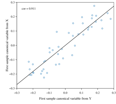
Figure 2: Scatter plot of the first pair of sample canonical variates for the limestone grassland community data.

Figure 2 plots the first pair of sample variates 𝝂1⊤​𝐗\boldsymbol{\nu}_{1}^{\top}{\bf X} and 𝝃1⊤​𝐘\boldsymbol{\xi}_{1}^{\top}{\bf Y}. The sample correlation between them is approximately

l1=0.9107.\sqrt{l_{1}}=0.9107.

The points display a clear positive linear trend, which is consistent with the large first squared canonical correlation. This plot describes the sample-level association between the two canonical variates. The plug-in estimator μ^1\hat{\mu}_{1}, on the other hand, provides an estimate of the population-level recovery quality: it measures how reliably the corresponding sample direction represents its population counterpart under the high-dimensional asymptotic framework.

This example illustrates the additional information provided by the proposed plug-in estimator. The inequality l1>d+l_{1}>d_{+} shows that the leading direction is detectable from the sample spectrum, but it does not by itself indicate whether the corresponding sample direction is a reliable representative of the population direction. The estimator μ^1\hat{\mu}_{1} addresses this second question. In the present dataset, μ^1=0.8155\hat{\mu}_{1}=0.8155 suggests that the leading sample canonical direction retains a substantial amount of population-level directional information. Thus, the proposed estimator does not merely restate the presence of a sample spiked eigenvalue; rather, it quantifies the recovery quality of the associated sample direction.

This distinction is important in the high-dimensional regime. Since sample canonical directions are generally not consistent estimators of their population counterparts, the direct recovery of the population directions is no longer the appropriate benchmark. A more relevant question is how much population-level structural information is preserved by the sample directions. Theorem 2.4 provides a quantitative answer to this question through the limit of the squared alignment, and Proposition 3.1 makes this quantity estimable from the data. In this sense, μ^i\hat{\mu}_{i} turns the non-consistency of sample canonical directions into a data-based measure of recovery quality, thereby complementing the usual eigenvalue-based detection of spiked directions.

4 Simulation

We conduct Monte Carlo simulations to examine the finite-sample performance of the first-order limit and the Gaussian fluctuation stated in Theorems 2.4 and 2.5. Throughout, we take p=⌊c1​n⌋p=\lfloor c_{1}n\rfloor and q=⌊c2​n⌋q=\lfloor c_{2}n\rfloor with (c1,c2)=(0.5,0.3)(c_{1},c_{2})=(0.5,0.3). The data matrices are generated under the Gaussian model: the entries {yi​j}\{y_{ij}\} and {wi​j}\{w_{ij}\} are independent and identically distributed (i.i.d.) as 𝒩​(0,1/n)\mathcal{N}(0,1/n). The simulations have two goals: to illustrate the convergence of ⟨𝒖i,𝝂i⟩2\langle{\boldsymbol{u}}_{i},\boldsymbol{\nu}_{i}\rangle^{2} to its deterministic limit, and to assess the normal approximation after the standardization in Theorem 2.5. For each value of nn, we repeat the experiment independently 50005000 times and compute ⟨𝒖i,𝝂i⟩2\langle{\boldsymbol{u}}_{i},\boldsymbol{\nu}_{i}\rangle^{2} in each repetition.

We consider two population canonical correlation structures. In the first setting, the population spike structure has rank one, with a single spike r1=0.8r_{1}=0.8. In the second setting, 𝚲​𝚲⊤\boldsymbol{\Lambda}\boldsymbol{\Lambda}^{\top} has rank three, with spikes r1=0.86r_{1}=0.86, r2=0.81r_{2}=0.81, and r3=0.76r_{3}=0.76. For (c1,c2)=(0.5,0.3)(c_{1},c_{2})=(0.5,0.3), the phase-transition threshold is

rc=c1​c2(1−c1)​(1−c2)≈0.655.r_{c}=\sqrt{\dfrac{c_{1}c_{2}}{(1-c_{1})(1-c_{2})}}\approx 0.655.

In both settings, the spikes are chosen above the phase-transition threshold, so that the associated sample eigenvalues separate from the bulk.

We first examine the deterministic limit in Theorem 2.4. For the rank-one setting, Figure 3 displays, for n∈{400,800,1200,1600,2000,2400,2800,3200,3600,4000}n\in\{400,800,1200,1600,2000,2400,2800,3200,3600,4000\}, the boxplots of ⟨𝒖1,𝝂1⟩2\langle{\boldsymbol{u}}_{1},\boldsymbol{\nu}_{1}\rangle^{2} over 50005000 repetitions, together with the corresponding Monte Carlo mean curve. As nn increases, the empirical distribution becomes more concentrated; both the interquartile range and the whiskers shrink. The Monte Carlo mean approaches the deterministic limit 1/(1+d​(r1))1/(1+d(r_{1})) predicted by Theorem 2.4. A mild finite-sample deviation from the theoretical limit is observed at small nn (e.g., n=400n=400), but it diminishes rapidly as nn grows, indicating a stable convergence to the theoretical limit.

Refer to caption
Figure 3: Rank-one setting: boxplots of ⟨𝒖1,𝝂1⟩2\langle{\boldsymbol{u}}_{1},\boldsymbol{\nu}_{1}\rangle^{2} over 50005000 repetitions for n∈{400,800,…,4000}n\in\{400,800,\ldots,4000\}, illustrating the first-order limit in Theorem 2.4.

We next investigate the fluctuation result in Theorem 2.5. Still in the rank-one setting, we fix a large sample size n=4000n=4000 and standardize ⟨𝒖1,𝝂1⟩2\langle{\boldsymbol{u}}_{1},\boldsymbol{\nu}_{1}\rangle^{2} according to Theorem 2.5:

Z1=n​(⟨𝒖1,𝝂1⟩2−1/(1+d​(r1)))σ​(r1)/(1+d​(r1))2.Z_{1}=\frac{\sqrt{n}\Big(\langle{\boldsymbol{u}}_{1},\boldsymbol{\nu}_{1}\rangle^{2}-1/(1+d(r_{1}))\Big)}{\sigma(r_{1})/(1+d(r_{1}))^{2}}.

Here and below, σ​(ri)=σ2​(ri)\sigma(r_{i})=\sqrt{\sigma^{2}(r_{i})}. Figure 4 shows the histogram of Z1Z_{1} based on 50005000 repetitions, overlaid with the 𝒩​(0,1)\mathcal{N}(0,1) density. The empirical histogram agrees well with the standard normal density, supporting the Gaussian approximation in Theorem 2.5 for large but finite nn.

Refer to caption
Figure 4: Rank-one setting: histogram of the standardized statistic Z1Z_{1} at n=4000n=4000 over 50005000 repetitions, overlaid with the 𝒩​(0,1)\mathcal{N}(0,1) density, supporting the Gaussian approximation in Theorem 2.5.

We then turn to the rank-three setting. For each spike rir_{i} (i=1,2,3)(i=1,2,3), we compute ⟨𝒖i,𝝂i⟩2\langle{\boldsymbol{u}}_{i},\boldsymbol{\nu}_{i}\rangle^{2} over repeated Monte Carlo simulations and plot the running empirical mean against the number of repetitions. Figure 5 displays the convergence trajectories together with the corresponding theoretical first-order limits. The three panels show that the running averages stabilize around their predicted limits, providing numerical support for the first-order asymptotic theory. The convergence behavior varies across the three spike components. In all three cases, the running empirical means fluctuate around their corresponding theoretical first-order limits and gradually stabilize as the number of repetitions increases. The components associated with stronger spikes, such as r1r_{1} and r2r_{2}, settle near their limiting values after the initial transient fluctuations. The weakest spike r3r_{3} displays a more pronounced initial deviation and a slower stabilization pattern. Overall, these numerical results are broadly consistent with the theoretical prediction that stronger spectral separation improves the stability of the associated squared alignment.

Refer to caption
(a) r1=0.86r_{1}=0.86
Refer to caption
(b) r2=0.81r_{2}=0.81
Refer to caption
(c) r3=0.76r_{3}=0.76
Figure 5: Rank-three setting: convergence trajectories of the running means of ⟨𝒖i,𝝂i⟩2\langle{\boldsymbol{u}}_{i},\boldsymbol{\nu}_{i}\rangle^{2} (i=1,2,3)(i=1,2,3) over 5000 repetitions, illustrating the first-order limits and the dependence on signal strength.

Finally, we assess the Gaussian fluctuation in the rank-three setting. For n∈{2000,4000,6000}n\in\{2000,4000,6000\}, we form the standardized statistics

Zi=n​(⟨𝒖i,𝝂i⟩2−1/(1+d​(ri)))σ​(ri)/(1+d​(ri))2,i=1,2,3,Z_{i}=\frac{\sqrt{n}\Big(\langle{\boldsymbol{u}}_{i},\boldsymbol{\nu}_{i}\rangle^{2}-1/(1+d(r_{i}))\Big)}{\sigma(r_{i})/(1+d(r_{i}))^{2}},\qquad i=1,2,3,

and repeat the experiment 50005000 times. Figures 6–8 provide three complementary diagnostics for the asymptotic normality of the standardized statistics ZiZ_{i} (i=1,2,3)(i=1,2,3) in the rank-three setting. Figure 6 shows the empirical histograms at n=2000n=2000, overlaid with the standard normal density. The histograms are centered near zero and exhibit an approximately bell-shaped profile, indicating that the normal approximation is already visible at this sample size. Figure 7 presents the corresponding Q-Q plots at n=4000n=4000. The sample quantiles lie close to the reference normal line for all three spiked components, which confirms the normal approximation from a quantile perspective. Mild deviations appear mainly in the tails, as is typical in finite-sample simulations. Figure 8 compares the empirical distribution functions at n=6000n=6000 with the standard normal distribution function. The empirical CDFs almost overlap with the theoretical CDF, showing good agreement at the level of the full distribution function. Overall, these graphical diagnostics demonstrate that the finite-sample behavior of the standardized statistics ZiZ_{i} is consistent with the asymptotic normality result established in Theorem 2.5.

Refer to caption
(a) r1=0.86,n=2000r_{1}=0.86,\,n=2000
Refer to caption
(b) r2=0.81,n=2000r_{2}=0.81,\,n=2000
Refer to caption
(c) r3=0.76,n=2000r_{3}=0.76,\,n=2000
Figure 6: Rank-three setting: histograms of the standardized statistics ZiZ_{i} (i=1,2,3i=1,2,3) at n=2000n=2000 over 50005000 repetitions, overlaid with the 𝒩​(0,1)\mathcal{N}(0,1) density.
Refer to caption
(a) r1=0.86,n=4000r_{1}=0.86,\,n=4000
Refer to caption
(b) r2=0.81,n=4000r_{2}=0.81,\,n=4000
Refer to caption
(c) r3=0.76,n=4000r_{3}=0.76,\,n=4000
Figure 7: Rank-three setting: Q-Q plots of the standardized statistics ZiZ_{i} (i=1,2,3)(i=1,2,3) at n=4000n=4000 against the standard normal distribution.
Refer to caption
(a) r1=0.86,n=6000r_{1}=0.86,\,n=6000
Refer to caption
(b) r2=0.81,n=6000r_{2}=0.81,\,n=6000
Refer to caption
(c) r3=0.76,n=6000r_{3}=0.76,\,n=6000
Figure 8: Rank-three setting: empirical distribution functions of the standardized statistics ZiZ_{i} (i=1,2,3)(i=1,2,3) at n=6000n=6000, compared with the standard normal distribution function.

5 Proof of Main Theorems

This section outlines the main proof strategy. We first use the characteristic equation to transform the eigenvector projection problem into a problem concerning quadratic forms of resolvent matrices. We then demonstrate how the proofs of our main results, Theorem 2.4 and 2.5, are reduced to the computation of the deterministic limits and fluctuations of these quadratic forms, which are established in the subsequent technical lemmas.

5.1 Schur Complement Reduction

Consider the following characteristic equation:

𝐒x​y​𝐒y​y−1​𝐒y​x​𝝂i=li​𝐒x​x​𝝂i,\displaystyle{\bf S}_{xy}{\bf S}_{yy}^{-1}{\bf S}_{yx}\boldsymbol{\nu}_{i}=l_{i}{\bf S}_{xx}\boldsymbol{\nu}_{i},

i.e.,

(𝐒x​y​𝐒y​y−1​𝐒y​x−li​𝐒x​x)​𝝂i=0,\displaystyle\left({\bf S}_{xy}{\bf S}_{yy}^{-1}{\bf S}_{yx}-l_{i}{\bf S}_{xx}\right)\boldsymbol{\nu}_{i}=0,

where lil_{i} is the ii-th eigenvalue of 𝐒x​x−1​𝐒x​y​𝐒y​y−1​𝐒y​x{\bf S}_{xx}^{-1}{\bf S}_{xy}{\bf S}_{yy}^{-1}{\bf S}_{yx}, and 𝝂i\boldsymbol{\nu}_{i} is the eigenvector corresponding to the eigenvalue lil_{i}. Using the model 𝐗=𝚲​𝐘+𝚪​𝐖{\bf X}=\boldsymbol{\Lambda}{\bf Y}+\boldsymbol{\Gamma}{\bf W} and the definitions of the sample covariance matrices, we can write 𝐒x​x=𝐗𝐗⊤{\bf S}_{xx}={\bf X}{\bf X}^{\top} and 𝐒x​y​𝐒y​y−1​𝐒y​x=𝐗𝐏y​𝐗⊤{\bf S}_{xy}{\bf S}_{yy}^{-1}{\bf S}_{yx}={\bf X}{\bf P}_{y}{\bf X}^{\top}, where 𝐏y=𝐘⊤​(𝐘𝐘⊤)−1​𝐘{\bf P}_{y}={\bf Y}^{\top}({\bf Y}{\bf Y}^{\top})^{-1}{\bf Y}. Note that 𝐏y{\bf P}_{y} is an orthogonal projector: 𝐏y⊤=𝐏y{\bf P}_{y}^{\top}={\bf P}_{y} and 𝐏y2=𝐏y{\bf P}_{y}^{2}={\bf P}_{y}. The equation becomes (𝐗𝐏y​𝐗⊤−li​𝐗𝐗⊤)​𝝂i=0\left({\bf X}{\bf P}_{y}{\bf X}^{\top}-l_{i}{\bf X}{\bf X}^{\top}\right)\boldsymbol{\nu}_{i}=0, or

𝐗​(𝐏y−li​𝐈n)​𝐗⊤​𝝂i=0.\displaystyle{\bf X}({\bf P}_{y}-l_{i}{\bf I}_{n}){\bf X}^{\top}\boldsymbol{\nu}_{i}=0.

Let 𝚲\boldsymbol{\Lambda} have the SVD 𝚲=𝐔​(𝚲k𝟎𝟎𝟎)​𝐕⊤\boldsymbol{\Lambda}={\bf U}\begin{pmatrix}\boldsymbol{\Lambda}_{k}&\mathbf{0}\\ \mathbf{0}&\mathbf{0}\end{pmatrix}{\bf V}^{\top}, where 𝐔=(𝐔1,𝐔2)∈ℝp×p{\bf U}=({\bf U}_{1},{\bf U}_{2})\in\mathbb{R}^{p\times p}, 𝐕=(𝐕1,𝐕2)∈ℝq×q{\bf V}=({\bf V}_{1},{\bf V}_{2})\in\mathbb{R}^{q\times q} are orthogonal, and 𝚲k∈ℝk×k\boldsymbol{\Lambda}_{k}\in\mathbb{R}^{k\times k} satisfies 𝚲k​𝚲k⊤=diag​(r1,…,rk)\boldsymbol{\Lambda}_{k}\boldsymbol{\Lambda}_{k}^{\top}=\mathrm{diag}(r_{1},\dots,r_{k}). We also write 𝚪=𝐔​diag​(𝚪k,𝐈p−k)​𝐔⊤\boldsymbol{\Gamma}={\bf U}\mathrm{diag}(\boldsymbol{\Gamma}_{k},{\bf I}_{p-k}){\bf U}^{\top} with 𝚪k=diag​(1−r1,…,1−rk)\boldsymbol{\Gamma}_{k}=\mathrm{diag}(\sqrt{1-r_{1}},\dots,\sqrt{1-r_{k}}). We further analyze the block matrix form of the characteristic equation. Let 𝐔=(𝐔1,𝐔2){\bf U}=({\bf U}_{1},{\bf U}_{2}) where 𝐔1{\bf U}_{1} consists of the first kk columns (the population spiked eigenvectors) and 𝐔2{\bf U}_{2} the remaining p−kp-k. Substituting the model for 𝐗{\bf X}, we have that 𝝂i\boldsymbol{\nu}_{i} satisfies

(𝐔1,𝐔2)​((𝚲k𝟎𝟎𝟎)​(𝐕1,𝐕2)⊤​𝐘+(𝚪k𝟎𝟎𝐈p−k)​𝐔⊤​𝐖)​(𝐏y−li​𝐈n)\displaystyle\left({\bf U}_{1},{\bf U}_{2}\right)\left(\begin{pmatrix}\boldsymbol{\Lambda}_{k}&\mathbf{0}\\ \mathbf{0}&\mathbf{0}{}\end{pmatrix}({\bf V}_{1},{\bf V}_{2})^{\top}{\bf Y}+\begin{pmatrix}\boldsymbol{\Gamma}_{k}&\mathbf{0}\\ \mathbf{0}&{\bf I}_{p-k}\end{pmatrix}{\bf U}^{\top}{\bf W}\right)({\bf P}_{y}-l_{i}{\bf I}_{n})
×(𝐘⊤(𝐕1,𝐕2)(𝚲k𝟎𝟎𝟎)+𝐖⊤𝐔(𝚪k𝟎𝟎𝐈p−k))(𝐔1⊤𝐔2⊤)𝝂i=0,\displaystyle~~~~~~~~~~~~~~~~~~~~~~~~\times\left({\bf Y}^{\top}({\bf V}_{1},{\bf V}_{2})\begin{pmatrix}\boldsymbol{\Lambda}_{k}&\mathbf{0}\\ \mathbf{0}&\mathbf{0}\end{pmatrix}+{\bf W}^{\top}{\bf U}\begin{pmatrix}\boldsymbol{\Gamma}_{k}&\mathbf{0}\\ \mathbf{0}&{\bf I}_{p-k}\end{pmatrix}\right)\begin{pmatrix}{\bf U}_{1}^{\top}{}\\ {\bf U}_{2}^{\top}\end{pmatrix}\boldsymbol{\nu}_{i}=0,

expanding this yields:

(𝐔1,𝐔2)​(𝐀𝐁𝐂𝐃)​(ϖi​1ϖi​2)=0,\displaystyle\left({\bf U}_{1},{\bf U}_{2}\right)\begin{pmatrix}{\bf A}&{\bf B}\\ {\bf C}&{\bf D}\end{pmatrix}\begin{pmatrix}\boldsymbol{\varpi}_{i1}\\ \boldsymbol{\varpi}_{i2}\end{pmatrix}=0,

where ϖi​1=𝐔1⊤​𝝂i\boldsymbol{\varpi}_{i1}={\bf U}_{1}^{\top}\boldsymbol{\nu}_{i} (a k×1k\times 1 vector) and ϖi​2=𝐔2⊤​𝝂i\boldsymbol{\varpi}_{i2}={\bf U}_{2}^{\top}\boldsymbol{\nu}_{i} (a (p−k)×1(p-k)\times 1 vector). The matrices are defined as

𝐀=𝐀​(li):=(𝚲k​𝐕1⊤​𝐘+𝚪k​𝐔1⊤​𝐖)​(𝐏y−li​𝐈n)​(𝐘⊤​𝐕1​𝚲k+𝐖⊤​𝐔1​𝚪k),\displaystyle{\bf A}={\bf A}(l_{i}):=(\boldsymbol{\Lambda}_{k}{\bf V}_{1}^{\top}{\bf Y}\!+\!\boldsymbol{\Gamma}_{k}{\bf U}_{1}^{\top}{\bf W})({\bf P}_{y}\!-\!l_{i}{\bf I}_{n})({\bf Y}^{\top}{\bf V}_{1}\boldsymbol{\Lambda}_{k}\!+\!{\bf W}^{\top}{\bf U}_{1}\boldsymbol{\Gamma}_{k}),
𝐁=𝐁​(li):=(𝚲k​𝐕1⊤​𝐘+𝚪k​𝐔1⊤​𝐖)​(𝐏y−li​𝐈n)​𝐖⊤​𝐔2,\displaystyle{\bf B}={\bf B}(l_{i}):=(\boldsymbol{\Lambda}_{k}{\bf V}_{1}^{\top}{\bf Y}\!+\!\boldsymbol{\Gamma}_{k}{\bf U}_{1}^{\top}{\bf W})({\bf P}_{y}\!-\!l_{i}{\bf I}_{n}){\bf W}^{\top}{\bf U}_{2},
𝐂=𝐂​(li):=𝐔2⊤​𝐖​(𝐏y−li​𝐈n)​(𝐘⊤​𝐕1​𝚲k+𝐖⊤​𝐔1​𝚪k),\displaystyle{\bf C}={\bf C}(l_{i}):={\bf U}_{2}^{\top}{\bf W}({\bf P}_{y}\!-\!l_{i}{\bf I}_{n})({\bf Y}^{\top}{\bf V}_{1}\boldsymbol{\Lambda}_{k}\!+\!{\bf W}^{\top}{\bf U}_{1}\boldsymbol{\Gamma}_{k}),
𝐃=𝐃​(li):=𝐔2⊤​𝐖​(𝐏y−li​𝐈n)​𝐖⊤​𝐔2.\displaystyle{\bf D}={\bf D}(l_{i}):={\bf U}_{2}^{\top}{\bf W}({\bf P}_{y}\!-\!l_{i}{\bf I}_{n}){\bf W}^{\top}{\bf U}_{2}.

Since lil_{i} is a sample spike and li→a.s.γil_{i}\xrightarrow{a.s.}\gamma_{i}, on an event whose probability tends to one, the matrix 𝐃​(li)=𝐔2⊤​𝐖​(𝐏y−li​𝐈n)​𝐖⊤​𝐔2{\bf D}(l_{i})={\bf U}_{2}^{\top}{\bf W}({\bf P}_{y}-l_{i}{\bf I}_{n}){\bf W}^{\top}{\bf U}_{2} is invertible. On this event, we may apply the Schur complement to the block matrix above.

(𝐔1,𝐔2)​(𝐈k𝐁𝐃−10𝐈p−k)​(𝐀−𝐁𝐃−1​𝐂𝟎𝟎𝐃)​(ϖi​1𝐃−1​𝐂​ϖi​1+ϖi​2)=0,\displaystyle\left({\bf U}_{1},{\bf U}_{2}\right)\begin{pmatrix}{\bf I}_{k}&{\bf B}{\bf D}^{-1}\\ 0&{\bf I}_{p-k}\end{pmatrix}\begin{pmatrix}{\bf A}-{\bf B}{\bf D}^{-1}{\bf C}&\mathbf{0}\\ \mathbf{0}&{\bf D}\end{pmatrix}\begin{pmatrix}\boldsymbol{\varpi}_{i1}{}\\ {\bf D}^{-1}{\bf C}\boldsymbol{\varpi}_{i1}+\boldsymbol{\varpi}_{i2}{}\end{pmatrix}=0,

This yields the equivalent system of equations:

{(𝐀−𝐁𝐃−1​𝐂)​ϖi​1=0,𝐂​ϖi​1+𝐃​ϖi​2=0,\displaystyle\left\{\begin{matrix}({\bf A}-{\bf B}{\bf D}^{-1}{\bf C})\boldsymbol{\varpi}_{i1}=0,\\ {\bf C}\boldsymbol{\varpi}_{i1}+{\bf D}\boldsymbol{\varpi}_{i2}=0,\end{matrix}\right.

which implies

{(𝐀−𝐁𝐃−1​𝐂)​ϖi​1=0,ϖi​2=−𝐃−1​𝐂​ϖi​1.\displaystyle\left\{\begin{matrix}({\bf A}-{\bf B}{\bf D}^{-1}{\bf C})\boldsymbol{\varpi}_{i1}=0,\\ \boldsymbol{\varpi}_{i2}=-{\bf D}^{-1}{\bf C}\boldsymbol{\varpi}_{i1}.\end{matrix}\right. (9)

The first equation determines the direction of ϖi​1\boldsymbol{\varpi}_{i1}, while the second equation links ϖi​2\boldsymbol{\varpi}_{i2} to ϖi​1\boldsymbol{\varpi}_{i1}. The vector of interest is ϖi​1\boldsymbol{\varpi}_{i1}, which contains the projections ⟨𝒖j,𝝂i⟩\langle{\boldsymbol{u}}_{j},\boldsymbol{\nu}_{i}\rangle for j=1,…,kj=1,\dots,k. Since 𝝂i\boldsymbol{\nu}_{i} has unit norm, we have ‖ϖi​1‖2+‖ϖi​2‖2=1\|\boldsymbol{\varpi}_{i1}\|^{2}+\|\boldsymbol{\varpi}_{i2}\|^{2}=1. Substituting the second equation of (9) gives the normalization constraint:

ϖi​1⊤​ϖi​1+ϖi​1⊤​𝐂⊤​(𝐃−1)⊤​𝐃−1​𝐂​ϖi​1=1.\displaystyle\boldsymbol{\varpi}_{i1}^{\top}\boldsymbol{\varpi}_{i1}+\boldsymbol{\varpi}_{i1}^{\top}{\bf C}^{\top}({\bf D}^{-1})^{\top}{\bf D}^{-1}{\bf C}\boldsymbol{\varpi}_{i1}=1.

Since 𝐃{\bf D} is symmetric, this simplifies to

ϖi​1⊤​(𝐈k+𝐂⊤​𝐃−2​𝐂)​ϖi​1=1.\displaystyle\boldsymbol{\varpi}_{i1}^{\top}\left({\bf I}_{k}+{\bf C}^{\top}{\bf D}^{-2}{\bf C}\right)\boldsymbol{\varpi}_{i1}=1. (10)

The kk-dimensional matrix 𝐀−𝐁𝐃−1​𝐂{\bf A}-{\bf B}{\bf D}^{-1}{\bf C} above is consistent with the content shown in equation (4.13) of Bao et al. (2019) [8]. Let

MΛ​(z):=𝐀​(z)−𝐁​(z)​𝐃​(z)−1​𝐂​(z)M_{\Lambda}(z):={\bf A}(z)-{\bf B}(z){\bf D}(z)^{-1}{\bf C}(z)

be the (random) k×kk\times k matrix-valued function arising from the Schur complement. For the ii-th sample outlier lil_{i} with limit γi\gamma_{i}, we invoke (6.9) of [8]. In particular, for α,β∈Ii\alpha,\beta\in I_{i} (the index set associated with the population spike rir_{i}), there exists a random matrix ℛ\mathcal{R} (defined in Lemma 6.2 of [8]) such that

(MΛ)α​β​(li)=Mα​β​(γi)−δα​β​Δi​i​(li−γi)​(1+op​(1))+1n​ℛα​β+op​(n−1/2),(M_{\Lambda})_{\alpha\beta}(l_{i})=M_{\alpha\beta}(\gamma_{i})-\delta_{\alpha\beta}\Delta_{ii}\,(l_{i}-\gamma_{i})\,(1+o_{p}(1))+\frac{1}{\sqrt{n}}\mathcal{R}_{\alpha\beta}+o_{p}(n^{-1/2}), (11)

where M​(z)M(z) is a deterministic diagonal matrix with diagonal entries mj​(z)m_{j}(z) and Δ\Delta is also diagonal. Moreover, mj​(γj)=0m_{j}(\gamma_{j})=0 for each jj. Let 𝒥i\mathcal{J}_{i} denote the index set of population eigenvalues equal to rir_{i}. For the simple spike rir_{i}, we have

(MΛ)i​i​(li)=Op​(n−1/2).(M_{\Lambda})_{ii}(l_{i})=O_{p}(n^{-1/2}).

Moreover, the off-diagonal blocks satisfy

(MΛ​(li))−i,i=Op​(n−1/2),(MΛ​(li))i,−i=Op​(n−1/2).(M_{\Lambda}(l_{i}))_{-i,i}=O_{p}(n^{-1/2}),\qquad(M_{\Lambda}(l_{i}))_{i,-i}=O_{p}(n^{-1/2}).

For j≠ij\neq i, since mj​(γi)≠0m_{j}(\gamma_{i})\neq 0, the diagonal entries of M​(γi)M(\gamma_{i}) in the (−i,−i)(-i,-i) block are bounded away from zero. Hence

(MΛ​(li))−i,−i=(M​(γi))−i,−i+Op​(n−1/2)(M_{\Lambda}(l_{i}))_{-i,-i}=(M(\gamma_{i}))_{-i,-i}+O_{p}(n^{-1/2})

is invertible with probability tending to one, and

‖(MΛ​(li))−i,−i−1‖=Op​(1).\|(M_{\Lambda}(l_{i}))_{-i,-i}^{-1}\|=O_{p}(1).

Therefore, from the equation MΛ​(li)​ϖi​1=0M_{\Lambda}(l_{i})\boldsymbol{\varpi}_{i1}=0 we obtain

ϖi​1,−i=−(MΛ​(li))−i,−i−1​(MΛ​(li))−i,i​ϖi​1,i=Op​(n−1/2)​ϖi​1,i,\boldsymbol{\varpi}_{i1,-i}=-(M_{\Lambda}(l_{i}))_{-i,-i}^{-1}(M_{\Lambda}(l_{i}))_{-i,i}\,\boldsymbol{\varpi}_{i1,i}=O_{p}(n^{-1/2})\,\boldsymbol{\varpi}_{i1,i},

which shows that all components of ϖi​1\boldsymbol{\varpi}_{i1} except the ii-th one are of order Op​(n−1/2)O_{p}(n^{-1/2}). Thus, under the simple spike assumption 𝒥i={i}\mathcal{J}_{i}=\{i\},

ϖi​1,−i=Op​(n−1/2)​ϖi​1,i.\boldsymbol{\varpi}_{i1,-i}=O_{p}(n^{-1/2})\,\boldsymbol{\varpi}_{i1,i}.

Since ‖𝝂i‖=1\|\boldsymbol{\nu}_{i}\|=1, we have ϖi​1,i=Op​(1)\boldsymbol{\varpi}_{i1,i}=O_{p}(1), and hence

‖ϖi​1,−i‖=Op​(n−1/2).\|\boldsymbol{\varpi}_{i1,-i}\|=O_{p}(n^{-1/2}).

Let

𝐌i:=𝐈k+𝐂⊤​𝐃−2​𝐂.{\bf M}_{i}:={\bf I}_{k}+{\bf C}^{\top}{\bf D}^{-2}{\bf C}.

From the Schur complement reduction, we have

ϖi​1⊤​𝐌i​ϖi​1=1.\boldsymbol{\varpi}_{i1}^{\top}{\bf M}_{i}\boldsymbol{\varpi}_{i1}=1.

Moreover, for a simple spike rir_{i},

ϖi​1,−i=Op​(n−1/2)​ϖi​1,i.\boldsymbol{\varpi}_{i1,-i}=O_{p}(n^{-1/2})\boldsymbol{\varpi}_{i1,i}.

Since ‖𝝂i‖=1\|\boldsymbol{\nu}_{i}\|=1, we have ϖi​1,i=Op​(1)\boldsymbol{\varpi}_{i1,i}=O_{p}(1), and hence

‖ϖi​1,−i‖=Op​(n−1/2).\|\boldsymbol{\varpi}_{i1,-i}\|=O_{p}(n^{-1/2}).

Define

𝐫i=ϖi​1−ϖi​1,i​𝐞i.\mathbf{r}_{i}=\boldsymbol{\varpi}_{i1}-\boldsymbol{\varpi}_{i1,i}{\bf e}_{i}.

Then the ii-th component of 𝐫i\mathbf{r}_{i} is zero and

ϖi​1=ϖi​1,i​𝐞i+𝐫i,‖𝐫i‖=Op​(n−1/2).\boldsymbol{\varpi}_{i1}=\boldsymbol{\varpi}_{i1,i}{\bf e}_{i}+\mathbf{r}_{i},\qquad\|\mathbf{r}_{i}\|=O_{p}(n^{-1/2}).

Substituting this decomposition into the normalization constraint gives

1=ϖi​1,i2​[𝐌i]i​i+2​ϖi​1,i​𝐞i⊤​𝐌i​𝐫i+𝐫i⊤​𝐌i​𝐫i.1=\boldsymbol{\varpi}_{i1,i}^{2}[{\bf M}_{i}]_{ii}+2\boldsymbol{\varpi}_{i1,i}{\bf e}_{i}^{\top}{\bf M}_{i}\mathbf{r}_{i}+\mathbf{r}_{i}^{\top}{\bf M}_{i}\mathbf{r}_{i}.

By Lemma 5.1, for j≠ij\neq i,

[𝐌i]i​j=Op​(n−1/2).[{\bf M}_{i}]_{ij}=O_{p}(n^{-1/2}).

Since the ii-th component of 𝐫i\mathbf{r}_{i} is zero and kk is fixed,

𝐞i⊤​𝐌i​𝐫i=∑j≠i[𝐌i]i​j​(𝐫i)j=Op​(n−1).{\bf e}_{i}^{\top}{\bf M}_{i}\mathbf{r}_{i}=\sum_{j\neq i}[{\bf M}_{i}]_{ij}(\mathbf{r}_{i})_{j}=O_{p}(n^{-1}).

Also, since ‖𝐌i‖=Op​(1)\|{\bf M}_{i}\|=O_{p}(1),

𝐫i⊤​𝐌i​𝐫i=Op​(n−1).\mathbf{r}_{i}^{\top}{\bf M}_{i}\mathbf{r}_{i}=O_{p}(n^{-1}).

Therefore,

1=ϖi​1,i2​[𝐌i]i​i+Op​(n−1).1=\boldsymbol{\varpi}_{i1,i}^{2}[{\bf M}_{i}]_{ii}+O_{p}(n^{-1}).

Recalling that

ϖi​1,i2=⟨𝒖i,𝝂i⟩2,\boldsymbol{\varpi}_{i1,i}^{2}=\langle{\boldsymbol{u}}_{i},\boldsymbol{\nu}_{i}\rangle^{2},

we obtain the strengthened normalization reduction

⟨𝒖i,𝝂i⟩2​[𝐌i]i​i=1+Op​(n−1).\langle{\boldsymbol{u}}_{i},\boldsymbol{\nu}_{i}\rangle^{2}[{\bf M}_{i}]_{ii}=1+O_{p}(n^{-1}).

This strengthened reduction is sufficient for both the first-order limit and the second-order fluctuation. Therefore, up to the order needed for the first- and second-order analysis, the behavior of ⟨𝒖i,𝝂i⟩2\langle{\boldsymbol{u}}_{i},\boldsymbol{\nu}_{i}\rangle^{2} is governed by the ii-th diagonal entry of 𝐌i{\bf M}_{i}. Recalling the definitions of matrices 𝐂{\bf C} and 𝐃{\bf D}, we obtain the decomposition:

𝐌i\displaystyle{\bf M}_{i}
=\displaystyle= 𝐈k\displaystyle{\bf I}_{k}
+𝚪k​𝐔1⊤​𝐖​(𝐏y−li​𝐈n)​𝐖⊤​𝐔2​(𝐔2⊤​𝐖​(𝐏y−li​𝐈n)​𝐖⊤​𝐔2)−2​𝐔2⊤​𝐖​(𝐏y−li​𝐈n)​𝐖⊤​𝐔1​𝚪k\displaystyle+\boldsymbol{\Gamma}_{k}{\bf U}_{1}^{\top}{\bf W}({\bf P}_{y}\!-\!l_{i}{\bf I}_{n}){\bf W}^{\top}{\bf U}_{2}\left({\bf U}_{2}^{\top}{\bf W}({\bf P}_{y}\!-\!l_{i}{\bf I}_{n}){\bf W}^{\top}{\bf U}_{2}\right)^{-2}{\bf U}_{2}^{\top}{\bf W}({\bf P}_{y}\!-\!l_{i}{\bf I}_{n}){\bf W}^{\top}{\bf U}_{1}\boldsymbol{\Gamma}_{k}
+𝚲k​𝐕1⊤​𝐘​(𝐏y−li​𝐈n)​𝐖⊤​𝐔2​(𝐔2⊤​𝐖​(𝐏y−li​𝐈n)​𝐖⊤​𝐔2)−2​𝐔2⊤​𝐖​(𝐏y−li​𝐈n)​𝐘⊤​𝐕1​𝚲k\displaystyle+\boldsymbol{\Lambda}_{k}{\bf V}_{1}^{\top}{\bf Y}({\bf P}_{y}\!-\!l_{i}{\bf I}_{n}){\bf W}^{\top}{\bf U}_{2}\left({\bf U}_{2}^{\top}{\bf W}({\bf P}_{y}\!-\!l_{i}{\bf I}_{n}){\bf W}^{\top}{\bf U}_{2}\right)^{-2}{\bf U}_{2}^{\top}{\bf W}({\bf P}_{y}\!-\!l_{i}{\bf I}_{n}){\bf Y}^{\top}{\bf V}_{1}\boldsymbol{\Lambda}_{k}
+𝚲k​𝐕1⊤​𝐘​(𝐏y−li​𝐈n)​𝐖⊤​𝐔2​(𝐔2⊤​𝐖​(𝐏y−li​𝐈n)​𝐖⊤​𝐔2)−2​𝐔2⊤​𝐖​(𝐏y−li​𝐈n)​𝐖⊤​𝐔1​𝚪k\displaystyle+\boldsymbol{\Lambda}_{k}{\bf V}_{1}^{\top}{\bf Y}({\bf P}_{y}\!-\!l_{i}{\bf I}_{n}){\bf W}^{\top}{\bf U}_{2}\left({\bf U}_{2}^{\top}{\bf W}({\bf P}_{y}\!-\!l_{i}{\bf I}_{n}){\bf W}^{\top}{\bf U}_{2}\right)^{-2}{\bf U}_{2}^{\top}{\bf W}({\bf P}_{y}\!-\!l_{i}{\bf I}_{n}){\bf W}^{\top}{\bf U}_{1}\boldsymbol{\Gamma}_{k}
+𝚪k​𝐔1⊤​𝐖​(𝐏y−li​𝐈n)​𝐖⊤​𝐔2​(𝐔2⊤​𝐖​(𝐏y−li​𝐈n)​𝐖⊤​𝐔2)−2​𝐔2⊤​𝐖​(𝐏y−li​𝐈n)​𝐘⊤​𝐕1​𝚲k\displaystyle+\boldsymbol{\Gamma}_{k}{\bf U}_{1}^{\top}{\bf W}({\bf P}_{y}\!-\!l_{i}{\bf I}_{n}){\bf W}^{\top}{\bf U}_{2}\left({\bf U}_{2}^{\top}{\bf W}({\bf P}_{y}\!-\!l_{i}{\bf I}_{n}){\bf W}^{\top}{\bf U}_{2}\right)^{-2}{\bf U}_{2}^{\top}{\bf W}({\bf P}_{y}\!-\!l_{i}{\bf I}_{n}){\bf Y}^{\top}{\bf V}_{1}\boldsymbol{\Lambda}_{k}
:=\displaystyle:= 𝐈k+Ik​1+Ik​2+Ik​3+Ik​4.\displaystyle{\bf I}_{k}+I_{k1}+I_{k2}+I_{k3}+I_{k4}. (12)

Here 𝐃−2{\bf D}^{-2} means 𝐃−1​𝐃−1{\bf D}^{-1}{\bf D}^{-1}. Our proofs now hinge on finding the limits and fluctuations of the diagonal elements of these four matrices.

5.2 Technical Lemmas

The Schur complement reduction above shows that the proofs of Theorems 2.4 and 2.5 depend on the asymptotic behavior of the entries of

𝐌i:=𝐈k+𝐂⊤​𝐃−2​𝐂.{\bf M}_{i}:={\bf I}_{k}+{\bf C}^{\top}{\bf D}^{-2}{\bf C}.

Using the decomposition

𝐌i=𝐈k+Ik​1+Ik​2+Ik​3+Ik​4,{\bf M}_{i}={\bf I}_{k}+I_{k1}+I_{k2}+I_{k3}+I_{k4},

we summarize the required deterministic limits, off-diagonal bounds, and fluctuation limits in the following two lemmas. Their proofs are given in Sections 6 and 7.

Lemma 5.1 (First-order expansion and off-diagonal control).

Under the assumptions of Theorem 2.4, fix a simple spike rir_{i}. Then the ii-th diagonal entry of 𝐌i{\bf M}_{i} satisfies

[𝐌i]i​i=1+d​(ri)+Op​(n−1/2),[{\bf M}_{i}]_{ii}=1+d(r_{i})+O_{p}(n^{-1/2}),

where d​(ri)d(r_{i}) is the deterministic function appearing in Theorem 2.4. Moreover,

[Ik​3]i​i=Op​(n−1/2),[Ik​4]i​i=Op​(n−1/2).[I_{k3}]_{ii}=O_{p}(n^{-1/2}),\qquad[I_{k4}]_{ii}=O_{p}(n^{-1/2}).

For any a≠ba\neq b, the off-diagonal entries satisfy

[Ik​j]a​b=Op​(n−1/2),j=1,2,3,4.[I_{kj}]_{ab}=O_{p}(n^{-1/2}),\qquad j=1,2,3,4.

Consequently,

[𝐌i]a​b=Op​(n−1/2),a≠b.[{\bf M}_{i}]_{ab}=O_{p}(n^{-1/2}),\qquad a\neq b.

In particular,

‖𝐌i‖=Op​(1).\|{\bf M}_{i}\|=O_{p}(1).

Let 𝒱k​1\mathcal{V}_{k1} and 𝒱k​2\mathcal{V}_{k2} denote the centered Op​(n−1/2)O_{p}(n^{-1/2}) fluctuation terms of [Ik​1]i​i[I_{k1}]_{ii} and [Ik​2]i​i[I_{k2}]_{ii}, respectively. More precisely, define

[𝒱k​1]i​i:=[Ik​1]i​i−𝔼​([Ik​1]i​i∣𝐘,𝐔2⊤​𝐖),[𝒱k​2]i​i:=[Ik​2]i​i−𝔼​([Ik​2]i​i∣𝐘,𝐔2⊤​𝐖),[\mathcal{V}_{k1}]_{ii}:=[I_{k1}]_{ii}-\mathbb{E}\!\left([I_{k1}]_{ii}\mid{\bf Y},{\bf U}_{2}^{\top}{\bf W}\right),\qquad[\mathcal{V}_{k2}]_{ii}:=[I_{k2}]_{ii}-\mathbb{E}\!\left([I_{k2}]_{ii}\mid{\bf Y},{\bf U}_{2}^{\top}{\bf W}\right),

so that 𝔼​([𝒱k​1]i​i∣𝐘,𝐔2⊤​𝐖)=𝔼​([𝒱k​2]i​i∣𝐘,𝐔2⊤​𝐖)=0\mathbb{E}([\mathcal{V}_{k1}]_{ii}\mid{\bf Y},{\bf U}_{2}^{\top}{\bf W})=\mathbb{E}([\mathcal{V}_{k2}]_{ii}\mid{\bf Y},{\bf U}_{2}^{\top}{\bf W})=0. The following lemma characterizes the limiting variances and covariances of all fluctuation terms.

Lemma 5.2 (Fluctuation of the normalization factor).

Under the assumptions of Theorem 2.5, let

Gi,n:=n​([𝐌i]i​i−1−d​(ri)).G_{i,n}:=\sqrt{n}\left([{\bf M}_{i}]_{ii}-1-d(r_{i})\right).

Then

Gi,n→𝐷𝒩​(0,σ2​(ri)).G_{i,n}\xrightarrow{D}\mathcal{N}(0,\sigma^{2}(r_{i})).

More precisely, let

X1​n:=n​[𝒱k​1]i​i,X2​n:=n​[𝒱k​2]i​i,X3​n:=n​[Ik​3+Ik​4]i​i.X_{1n}:=\sqrt{n}[\mathcal{V}_{k1}]_{ii},\qquad X_{2n}:=\sqrt{n}[\mathcal{V}_{k2}]_{ii},\qquad X_{3n}:=\sqrt{n}[I_{k3}+I_{k4}]_{ii}.

Then

(X1​n,X2​n,X3​n)(X_{1n},X_{2n},X_{3n})

converges jointly in distribution to a centered Gaussian vector. Moreover,

Gi,n=X1​n+X2​n+X3​n+op​(1).G_{i,n}=X_{1n}+X_{2n}+X_{3n}+o_{p}(1).

The limiting variances are

Var⁡(X1​n)=A1​(ri)+o​(1),\operatorname{Var}(X_{1n})=A_{1}(r_{i})+o(1),

where

A1​(ri)=\displaystyle A_{1}(r_{i})= 2​(1−ri)2​P1​(ri)−4​η​ri−ωri​(1−ri)3​(P1​(ri)+F3​(ri))\displaystyle 2(1-r_{i})^{2}P_{1}(r_{i})-4\frac{\eta r_{i}-\omega}{r_{i}}(1-r_{i})^{3}(P_{1}(r_{i})+F_{3}(r_{i}))
+2​(η​ri−ω)2ri2​(1−ri)4​(P1​(ri)+2​F3​(ri)+Q3​(ri)),\displaystyle+\frac{2(\eta r_{i}-\omega)^{2}}{r_{i}^{2}}(1-r_{i})^{4}(P_{1}(r_{i})+2F_{3}(r_{i})+Q_{3}(r_{i})),
Var⁡(X2​n)=A2​(ri)+o​(1),\operatorname{Var}(X_{2n})=A_{2}(r_{i})+o(1),

where

A2​(ri)=2​(η​ri−ω)4​(1−ri)4ri2​(Jk​1​(ri)+Jk​2​(ri)+Jk​3​(ri)+Jk​4​(ri)+Jk​5​(ri)),A_{2}(r_{i})=\frac{2(\eta r_{i}-\omega)^{4}(1-r_{i})^{4}}{r_{i}^{2}}\left(J_{k1}(r_{i})+J_{k2}(r_{i})+J_{k3}(r_{i})+J_{k4}(r_{i})+J_{k5}(r_{i})\right),

and

Var⁡(X3​n)=A3​(ri)+o​(1),\operatorname{Var}(X_{3n})=A_{3}(r_{i})+o(1),

where

A3​(ri)=4​(η​ri−ω)3​(1−ri)4​Q4​(ri)c2​ri2+4​c1​(η​ri−ω)2​(1−ri)3​Q7​(ri)c2​ri.A_{3}(r_{i})=\frac{4(\eta r_{i}-\omega)^{3}(1-r_{i})^{4}Q_{4}(r_{i})}{c_{2}r_{i}^{2}}+\frac{4c_{1}(\eta r_{i}-\omega)^{2}(1-r_{i})^{3}Q_{7}(r_{i})}{c_{2}r_{i}}.

The scaled cross-covariances satisfy

Cov⁡(X1​n,X2​n)=o​(1),Cov⁡(X1​n,X3​n)=o​(1),Cov⁡(X2​n,X3​n)=o​(1).\operatorname{Cov}(X_{1n},X_{2n})=o(1),\qquad\operatorname{Cov}(X_{1n},X_{3n})=o(1),\qquad\operatorname{Cov}(X_{2n},X_{3n})=o(1).

Therefore,

σ2​(ri)=A1​(ri)+A2​(ri)+A3​(ri).\sigma^{2}(r_{i})=A_{1}(r_{i})+A_{2}(r_{i})+A_{3}(r_{i}).

The deterministic quantities

P1​(ri),F3​(ri),Q3​(ri),Jk​ℓ​(ri),ℓ=1,…,5,Q4​(ri),Q7​(ri)P_{1}(r_{i}),\quad F_{3}(r_{i}),\quad Q_{3}(r_{i}),\quad J_{k\ell}(r_{i}),\ \ell=1,\ldots,5,\quad Q_{4}(r_{i}),\quad Q_{7}(r_{i})

are defined in Section 7.

5.3 Proofs of Main Results

We now prove the main theorems, assuming Lemmas 5.1 and 5.2 hold.

Proof of Theorem 2.4.

By Lemma 5.1,

[𝐌i]i​i=1+d​(ri)+Op​(n−1/2).[{\bf M}_{i}]_{ii}=1+d(r_{i})+O_{p}(n^{-1/2}).

Together with the strengthened normalization reduction,

⟨𝒖i,𝝂i⟩2​[𝐌i]i​i=1+Op​(n−1),\langle{\boldsymbol{u}}_{i},\boldsymbol{\nu}_{i}\rangle^{2}[{\bf M}_{i}]_{ii}=1+O_{p}(n^{-1}),

we have

⟨𝒖i,𝝂i⟩2=1+Op​(n−1)1+d​(ri)+Op​(n−1/2).\langle{\boldsymbol{u}}_{i},\boldsymbol{\nu}_{i}\rangle^{2}=\frac{1+O_{p}(n^{-1})}{1+d(r_{i})+O_{p}(n^{-1/2})}.

Since 1+d​(ri)>01+d(r_{i})>0, the continuous mapping theorem gives

⟨𝒖i,𝝂i⟩2→𝑝11+d​(ri).\langle{\boldsymbol{u}}_{i},\boldsymbol{\nu}_{i}\rangle^{2}\xrightarrow{p}\frac{1}{1+d(r_{i})}.

This proves Theorem 2.4. ∎

Proof of Theorem 2.5.

By Lemma 5.2, we have

[𝐌i]i​i=1+d​(ri)+n−1/2​Gi,n+op​(n−1/2),[{\bf M}_{i}]_{ii}=1+d(r_{i})+n^{-1/2}G_{i,n}+o_{p}(n^{-1/2}),

where

Gi,n→𝐷𝒩​(0,σ2​(ri)).G_{i,n}\xrightarrow{D}\mathcal{N}(0,\sigma^{2}(r_{i})).

Using the strengthened normalization reduction,

⟨𝒖i,𝝂i⟩2​[𝐌i]i​i=1+Op​(n−1),\langle{\boldsymbol{u}}_{i},\boldsymbol{\nu}_{i}\rangle^{2}[{\bf M}_{i}]_{ii}=1+O_{p}(n^{-1}),

we obtain

⟨𝒖i,𝝂i⟩2=1+Op​(n−1)1+d​(ri)+n−1/2​Gi,n+op​(n−1/2).\langle{\boldsymbol{u}}_{i},\boldsymbol{\nu}_{i}\rangle^{2}=\frac{1+O_{p}(n^{-1})}{1+d(r_{i})+n^{-1/2}G_{i,n}+o_{p}(n^{-1/2})}.

Since 1+d​(ri)>01+d(r_{i})>0, a first-order Taylor expansion yields

⟨𝒖i,𝝂i⟩2=11+d​(ri)−n−1/2​Gi,n(1+d​(ri))2+op​(n−1/2).\langle{\boldsymbol{u}}_{i},\boldsymbol{\nu}_{i}\rangle^{2}=\frac{1}{1+d(r_{i})}-\frac{n^{-1/2}G_{i,n}}{(1+d(r_{i}))^{2}}+o_{p}(n^{-1/2}).

Therefore,

n​(⟨𝒖i,𝝂i⟩2−11+d​(ri))=−Gi,n(1+d​(ri))2+op​(1).\sqrt{n}\left(\langle{\boldsymbol{u}}_{i},\boldsymbol{\nu}_{i}\rangle^{2}-\frac{1}{1+d(r_{i})}\right)=-\frac{G_{i,n}}{(1+d(r_{i}))^{2}}+o_{p}(1).

Since

Gi,n→𝐷𝒩​(0,σ2​(ri)),G_{i,n}\xrightarrow{D}\mathcal{N}(0,\sigma^{2}(r_{i})),

Slutsky’s theorem implies

n​(⟨𝒖i,𝝂i⟩2−11+d​(ri))→𝐷𝒩​(0,σ2​(ri)(1+d​(ri))4).\sqrt{n}\left(\langle{\boldsymbol{u}}_{i},\boldsymbol{\nu}_{i}\rangle^{2}-\frac{1}{1+d(r_{i})}\right)\xrightarrow{D}\mathcal{N}\left(0,\frac{\sigma^{2}(r_{i})}{(1+d(r_{i}))^{4}}\right).

This proves Theorem 2.5. ∎

6 Proofs of Technical Lemmas

This section provides the proofs for the key technical lemmas, 5.1 and 5.2.

Proof of Lemma 5.1.

Based on the decomposition in Section 5, write

Ik​1=𝚪k​𝐔1⊤​𝐖​(𝐏y−li​𝐈n)​𝐖⊤​𝐔2​Φ2​(li)​𝐔2⊤​𝐖​(𝐏y−li​𝐈n)​𝐖⊤​𝐔1​𝚪k,I_{k1}=\boldsymbol{\Gamma}_{k}{\bf U}_{1}^{\top}{\bf W}({\bf P}_{y}-l_{i}{\bf I}_{n}){\bf W}^{\top}{\bf U}_{2}\Phi^{2}(l_{i}){\bf U}_{2}^{\top}{\bf W}({\bf P}_{y}-l_{i}{\bf I}_{n}){\bf W}^{\top}{\bf U}_{1}\boldsymbol{\Gamma}_{k},

where

Φ​(z)=(𝐔2⊤​𝐖​(𝐏y−z​𝐈n)​𝐖⊤​𝐔2)−1.\Phi(z)=\left({\bf U}_{2}^{\top}{\bf W}({\bf P}_{y}-z{\bf I}_{n}){\bf W}^{\top}{\bf U}_{2}\right)^{-1}.

Conditional on 𝐘{\bf Y} and 𝐔2⊤​𝐖{\bf U}_{2}^{\top}{\bf W}, the rows of 𝐔1⊤​𝐖{\bf U}_{1}^{\top}{\bf W} are independent centered Gaussian vectors with covariance n−1​𝐈nn^{-1}{\bf I}_{n}. Hence

𝔼​(Ik​1∣𝐘,𝐔2⊤​𝐖)=1n​tr​[(𝐏y−li​𝐈n)​𝐖⊤​𝐔2​Φ2​(li)​𝐔2⊤​𝐖​(𝐏y−li​𝐈n)]​𝚪k​𝚪k⊤.\mathbb{E}\!\left(I_{k1}\mid{\bf Y},{\bf U}_{2}^{\top}{\bf W}\right)=\frac{1}{n}{\rm tr}\!\left[({\bf P}_{y}-l_{i}{\bf I}_{n}){\bf W}^{\top}{\bf U}_{2}\Phi^{2}(l_{i}){\bf U}_{2}^{\top}{\bf W}({\bf P}_{y}-l_{i}{\bf I}_{n})\right]\boldsymbol{\Gamma}_{k}\boldsymbol{\Gamma}_{k}^{\top}.

Define

𝒱k​1:=Ik​1−𝔼​(Ik​1∣𝐘,𝐔2⊤​𝐖).\mathcal{V}_{k1}:=I_{k1}-\mathbb{E}\!\left(I_{k1}\mid{\bf Y},{\bf U}_{2}^{\top}{\bf W}\right).

Then

Ik​1=1n​tr​[(𝐏y−li​𝐈n)​𝐖⊤​𝐔2​Φ2​(li)​𝐔2⊤​𝐖​(𝐏y−li​𝐈n)]​𝚪k​𝚪k⊤+𝒱k​1.I_{k1}=\frac{1}{n}{\rm tr}\!\left[({\bf P}_{y}-l_{i}{\bf I}_{n}){\bf W}^{\top}{\bf U}_{2}\Phi^{2}(l_{i}){\bf U}_{2}^{\top}{\bf W}({\bf P}_{y}-l_{i}{\bf I}_{n})\right]\boldsymbol{\Gamma}_{k}\boldsymbol{\Gamma}_{k}^{\top}+\mathcal{V}_{k1}.

Under the Gaussian assumption on the entries of 𝐖{\bf W} and the orthogonality of 𝐔1{\bf U}_{1} and 𝐔2{\bf U}_{2}, it follows that 𝐔1⊤​𝐖{\bf U}_{1}^{\top}{\bf W} and 𝐔2⊤​𝐖{\bf U}_{2}^{\top}{\bf W} are independent. Moreover, by the proof of Theorem 1.1 in Bai and Silverstein (2004) [2], we have 𝒱k​1=Op​(n−1/2)\mathcal{V}_{k1}=O_{p}(n^{-1/2}). Throughout the proof, we adopt the standard normalization that the entries of 𝐖{\bf W} are i.i.d. N​(0,1/n)N(0,1/n).

Let Φ​(z)=(𝐔2⊤​𝐖​(𝐏y−z​𝐈n)​𝐖⊤​𝐔2)−1\Phi(z)=\left({\bf U}_{2}^{\top}{\bf W}({\bf P}_{y}\!-\!z{\bf I}_{n}){\bf W}^{\top}{\bf U}_{2}\right)^{-1}. Note that n​𝐄=n​𝐔2⊤​𝐖𝐏y​𝐖⊤​𝐔2∼𝒲p−k​(𝐈p−k,q)n{\bf E}=n{\bf U}_{2}^{\top}{\bf W}{\bf P}_{y}{\bf W}^{\top}{\bf U}_{2}\sim\mathcal{W}_{p-k}({\bf I}_{p-k},q) and n​𝐇=n​𝐔2⊤​𝐖​(𝐈−𝐏y)​𝐖⊤​𝐔2∼𝒲p−k​(𝐈p−k,n−q)n{\bf H}=n{\bf U}_{2}^{\top}{\bf W}({\bf I}-{\bf P}_{y}){\bf W}^{\top}{\bf U}_{2}\sim\mathcal{W}_{p-k}({\bf I}_{p-k},n-q). Hence Φ​(z)=((1−z)​𝐄−z​𝐇)−1\Phi(z)=\left((1-z){\bf E}-z{\bf H}\right)^{-1}. Consequently,

1n​tr​(𝐏y−li)​𝐖⊤​𝐔2​(𝐔2⊤​𝐖​(𝐏y−li)​𝐖⊤​𝐔2)−2​𝐔2⊤​𝐖​(𝐏y−li)\displaystyle\frac{1}{n}\text{tr}({\bf P}_{y}\!-\!l_{i}){\bf W}^{\top}{\bf U}_{2}\left({\bf U}_{2}^{\top}{\bf W}({\bf P}_{y}\!-\!l_{i}){\bf W}^{\top}{\bf U}_{2}\right)^{-2}{\bf U}_{2}^{\top}{\bf W}({\bf P}_{y}\!-\!l_{i})
=\displaystyle= (1−li)2​1n​tr​𝐄​Φ2​(li)+li2​1n​tr​𝐇​Φ2​(li).\displaystyle(1\!-\!l_{i})^{2}\frac{1}{n}\text{tr}{\bf E}\Phi^{2}(l_{i})\!+\!l_{i}^{2}\frac{1}{n}\text{tr}{\bf H}\Phi^{2}(l_{i}).

Differentiating with respect to zz yields

{(1n​tr​Φ​(li))′=1n​tr​Φ​(li)​(𝐄+𝐇)​Φ​(li),1n​tr​Φ​(li)=1−lin​tr​𝐄​Φ2−lin​tr​𝐇​Φ2​(li),\left\{\begin{aligned} \left(\frac{1}{n}\text{tr}\Phi(l_{i})\right)^{\prime}&=\frac{1}{n}\text{tr}\Phi(l_{i})({\bf E}+{\bf H})\Phi(l_{i}),\\ \frac{1}{n}\text{tr}\Phi(l_{i})&=\frac{1-l_{i}}{n}\text{tr}{\bf E}\Phi^{2}-\frac{l_{i}}{n}\text{tr}{\bf H}\Phi^{2}(l_{i}),\\ \end{aligned}\right.

that is,

{1n​tr​𝐄​Φ2​(li)=1n​tr​Φ​(li)+li​(1n​tr​Φ​(li))′,1n​tr​𝐇​Φ2​(li)=(1−li)​(1n​tr​Φ​(li))′−1n​tr​Φ​(li).\left\{\begin{aligned} \frac{1}{n}\text{tr}{\bf E}\Phi^{2}(l_{i})&=\frac{1}{n}\text{tr}\Phi(l_{i})+l_{i}\left(\frac{1}{n}\text{tr}\Phi(l_{i})\right)^{\prime},\\ \frac{1}{n}\text{tr}{\bf H}\Phi^{2}(l_{i})&=(1-l_{i})\left(\frac{1}{n}\text{tr}\Phi(l_{i})\right)^{\prime}-\frac{1}{n}\text{tr}\Phi(l_{i}).\\ \end{aligned}\right.

Therefore, it suffices to estimate the two key quantities n−1​tr​Φ​(li)n^{-1}\text{tr}\Phi(l_{i}) and (n−1​tr​Φ​(li))′\bigl(n^{-1}\text{tr}\Phi(l_{i})\bigr)^{\prime}.

Let 𝒳(p−k)×q\mathcal{X}_{(p-k)\times q} and 𝒴(p−k)×(n−q)\mathcal{Y}_{(p-k)\times(n-q)} be independent matrices with i.i.d. standard normal entries. Since

Φ​(z)=((1−z)​𝐄−z​𝐇)−1=n​((1−z)​n​𝐄−z​n​𝐇)−1,\Phi(z)=\left((1-z){\bf E}-z{\bf H}\right)^{-1}=n\left((1-z)n{\bf E}-zn{\bf H}\right)^{-1},

we have

1n​tr​Φ​(z)=11−z​tr​(n​𝐄−z1−z​n​𝐇)−1.\frac{1}{n}{\rm tr}\Phi(z)=\frac{1}{1-z}{\rm tr}\left(n{\bf E}-\frac{z}{1-z}n{\bf H}\right)^{-1}.

Therefore,

1n​tr​Φ​(z)​=𝑑​11−z​tr​(𝒳​𝒳⊤−z1−z​𝒴​𝒴⊤)−1.\frac{1}{n}{\rm tr}\Phi(z)\overset{d}{=}\frac{1}{1-z}{\rm tr}\left(\mathcal{X}\mathcal{X}^{\top}-\frac{z}{1-z}\mathcal{Y}\mathcal{Y}^{\top}\right)^{-1}.

Applying the Poincaré inequality in Lemma 2.3, we obtain the variance bound

Var⁡(tr​Φ​(z))\displaystyle\operatorname{Var}(\text{tr}\Phi(z))
≤\displaystyle\leq 𝔼​1n​∑i=1p−k∑j=1n−q[∂tr​Φ​(z)∂𝓎i​j]2+𝔼​1n​∑i=1p−k∑j=1q[∂tr​Φ​(z)∂𝓍i​j]2=O​(p+qn).\displaystyle\mathbb{E}\frac{1}{n}\sum_{i=1}^{p-k}\sum_{j=1}^{n-q}\left[\frac{\partial\text{tr}\Phi(z)}{\partial\mathcal{y}_{ij}}\right]^{2}+\mathbb{E}\frac{1}{n}\sum_{i=1}^{p-k}\sum_{j=1}^{q}\left[\frac{\partial\text{tr}\Phi(z)}{\partial\mathcal{x}_{ij}}\right]^{2}=O\left(\frac{p+q}{n}\right). (13)

The Poincaré inequality gives

Var⁡(tr​Φ​(z))=O​(1),\operatorname{Var}({\rm tr}\Phi(z))=O(1),

uniformly for zz in a compact set away from the limiting spectral support. Hence

1n​tr​Φ​(z)−𝔼​1n​tr​Φ​(z)=Op​(n−1).\frac{1}{n}{\rm tr}\Phi(z)-\mathbb{E}\frac{1}{n}{\rm tr}\Phi(z)=O_{p}(n^{-1}).

Combining this with the cumulant expansion formula in Lemma 2.2, we obtain

𝔼​tr​(𝒳​𝒳⊤​(𝒴​𝒴⊤)−1−z​𝐈p−k)−1\displaystyle\mathbb{E}\text{tr}(\mathcal{X}\mathcal{X}^{\top}(\mathcal{Y}\mathcal{Y}^{\top})^{-1}-z{\bf I}_{p-k})^{-1}
=\displaystyle= 𝔼​tr​𝒴​𝒴⊤​(𝒳​𝒳⊤−z​𝒴​𝒴⊤)−1\displaystyle\mathbb{E}\text{tr}\mathcal{Y}\mathcal{Y}^{\top}(\mathcal{X}\mathcal{X}^{\top}-z\mathcal{Y}\mathcal{Y}^{\top})^{-1}
=\displaystyle= 𝔼​1n​∑a=1p−k∑b=1n−qya​b​[𝒴⊤​(𝒳​𝒳⊤−z​𝒴​𝒴⊤)−1]b​a\displaystyle\mathbb{E}\frac{1}{n}\sum_{a=1}^{p-k}\sum_{b=1}^{n-q}y_{ab}\left[\mathcal{Y}^{\top}(\mathcal{X}\mathcal{X}^{\top}-z\mathcal{Y}\mathcal{Y}^{\top})^{-1}\right]_{ba}
=\displaystyle= n−qn​𝔼​tr​(𝒳​𝒳⊤−z​𝒴​𝒴⊤)−1+zn​𝔼​tr​(𝒳​𝒳⊤​(𝒴​𝒴⊤)−1−z​𝐈p−k)−1​tr​(𝒳​𝒳⊤−z​𝒴​𝒴⊤)−1+O​(1)\displaystyle\frac{n-q}{n}\mathbb{E}\text{tr}(\mathcal{X}\mathcal{X}^{\top}\!-\!z\mathcal{Y}\mathcal{Y}^{\top})^{-1}\!+\!\frac{z}{n}\mathbb{E}\text{tr}(\mathcal{X}\mathcal{X}^{\top}(\mathcal{Y}\mathcal{Y}^{\top})^{-1}\!-\!z{\bf I}_{p-k})^{-1}\text{tr}(\mathcal{X}\mathcal{X}^{\top}\!-\!z\mathcal{Y}\mathcal{Y}^{\top})^{-1}\!+\!O(1)
=\displaystyle= n−qn​𝔼​tr​(𝒳​𝒳⊤−z​𝒴​𝒴⊤)−1+zn​𝔼​tr​(𝒳​𝒳⊤​(𝒴​𝒴⊤)−1−z​𝐈p−k)−1​𝔼​tr​(𝒳​𝒳⊤−z​𝒴​𝒴⊤)−1+O​(1),\displaystyle\frac{n-q}{n}\mathbb{E}\text{tr}(\mathcal{X}\mathcal{X}^{\top}\!\!-\!\!z\mathcal{Y}\mathcal{Y}^{\top})^{-1}\!+\!\frac{z}{n}\mathbb{E}\text{tr}(\mathcal{X}\mathcal{X}^{\top}(\mathcal{Y}\mathcal{Y}^{\top})^{-1}\!\!-\!z{\bf I}_{p-k})^{-1}\mathbb{E}\text{tr}(\mathcal{X}\mathcal{X}^{\top}\!\!-\!\!z\mathcal{Y}\mathcal{Y}^{\top})^{-1}\!+\!O(1),

where the last equality follows from the Cauchy–Schwarz inequality. Consequently,

|𝔼1ntr(𝒳𝒳⊤(𝒴𝒴⊤)−1−z𝐈)−1tr(𝒳𝒳⊤−z𝒴𝒴⊤)−1\displaystyle\left|\mathbb{E}\frac{1}{n}\text{tr}(\mathcal{X}\mathcal{X}^{\top}(\mathcal{Y}\mathcal{Y}^{\top})^{-1}-z{\bf I})^{-1}\text{tr}(\mathcal{X}\mathcal{X}^{\top}-z\mathcal{Y}\mathcal{Y}^{\top})^{-1}\right.
−𝔼1ntr(𝒳𝒳⊤(𝒴𝒴⊤)−1−z𝐈)−1𝔼tr(𝒳𝒳⊤−z𝒴𝒴⊤)−1|\displaystyle~~~~~~~~~~~~~~~~~~~~~~~~~~\left.-\mathbb{E}\frac{1}{n}\text{tr}(\mathcal{X}\mathcal{X}^{\top}(\mathcal{Y}\mathcal{Y}^{\top})^{-1}-z{\bf I})^{-1}\mathbb{E}\text{tr}(\mathcal{X}\mathcal{X}^{\top}-z\mathcal{Y}\mathcal{Y}^{\top})^{-1}\right|
=\displaystyle= |𝔼​(1−𝔼)​1n​tr​(𝒳​𝒳⊤​(𝒴​𝒴⊤)−1−z​𝐈)−1​(1−𝔼)​tr​(𝒳​𝒳⊤−z​𝒴​𝒴⊤)−1|\displaystyle\left|\mathbb{E}(1-\mathbb{E})\frac{1}{n}\text{tr}(\mathcal{X}\mathcal{X}^{\top}(\mathcal{Y}\mathcal{Y}^{\top})^{-1}-z{\bf I})^{-1}(1-\mathbb{E})\text{tr}(\mathcal{X}\mathcal{X}^{\top}-z\mathcal{Y}\mathcal{Y}^{\top})^{-1}\right|
≤\displaystyle\leq 𝔼​|(1−𝔼)​1n​tr​(𝒳​𝒳⊤​(𝒴​𝒴⊤)−1−z​𝐈)−1|2​𝔼​|(1−𝔼)​tr​(𝒳​𝒳⊤−z​𝒴​𝒴⊤)−1|2\displaystyle\sqrt{\mathbb{E}\left|(1-\mathbb{E})\frac{1}{n}\text{tr}(\mathcal{X}\mathcal{X}^{\top}(\mathcal{Y}\mathcal{Y}^{\top})^{-1}-z{\bf I})^{-1}\right|^{2}}\sqrt{\mathbb{E}\left|(1-\mathbb{E})\text{tr}(\mathcal{X}\mathcal{X}^{\top}-z\mathcal{Y}\mathcal{Y}^{\top})^{-1}\right|^{2}}
≤\displaystyle\leq O​(1n).\displaystyle O\left(\frac{1}{n}\right).

Here the replacement of 𝔼​(tr​𝐀​tr​𝐁)\mathbb{E}({\rm tr}{\bf A}\,{\rm tr}{\bf B}) by 𝔼​tr​𝐀​𝔼​tr​𝐁\mathbb{E}{\rm tr}{\bf A}\,\mathbb{E}{\rm tr}{\bf B} introduces an O​(1)O(1) error, since by the Poincaré inequality both Var⁡(tr​𝐀)\operatorname{Var}({\rm tr}{\bf A}) and Var⁡(tr​B)\operatorname{Var}({\rm tr}B) are uniformly bounded, and hence the covariance is O​(1)O(1). After dividing by nn, this error becomes O​(1/n)O(1/n).

It follows that

𝔼​tr​(𝒳​𝒳⊤−z​𝒴​𝒴⊤)−1=𝔼​tr​(𝒳​𝒳⊤​(𝒴​𝒴⊤)−1−z​𝐈)−1n−qn+zn​𝔼​tr​(𝒳​𝒳⊤​(𝒴​𝒴⊤)−1−z​𝐈)−1+O​(1),\displaystyle\mathbb{E}\text{tr}(\mathcal{X}\mathcal{X}^{\top}-z\mathcal{Y}\mathcal{Y}^{\top})^{-1}=\frac{\mathbb{E}\text{tr}(\mathcal{X}\mathcal{X}^{\top}(\mathcal{Y}\mathcal{Y}^{\top})^{-1}-z{\bf I})^{-1}}{\frac{n-q}{n}+\frac{z}{n}\mathbb{E}\text{tr}(\mathcal{X}\mathcal{X}^{\top}(\mathcal{Y}\mathcal{Y}^{\top})^{-1}-z{\bf I})^{-1}}+O(1),

and hence

1n​tr​Φ​(z)=\displaystyle\frac{1}{n}\text{tr}\Phi(z)= 11−z​1n​𝔼​tr​(𝒳​𝒳⊤​(𝒴​𝒴⊤)−1−z1−z​𝐈)−1n−qn+z1−z​1n​𝔼​tr​(𝒳​𝒳⊤​(𝒴​𝒴⊤)−1−z1−z​𝐈)−1+Op​(1n)\displaystyle\frac{1}{1-z}\frac{\frac{1}{n}\mathbb{E}\text{tr}\left(\mathcal{X}\mathcal{X}^{\top}(\mathcal{Y}\mathcal{Y}^{\top})^{-1}-\frac{z}{1-z}{\bf I}\right)^{-1}}{\frac{n-q}{n}+\frac{z}{1-z}\frac{1}{n}\mathbb{E}\text{tr}\left(\mathcal{X}\mathcal{X}^{\top}(\mathcal{Y}\mathcal{Y}^{\top})^{-1}-\frac{z}{1-z}{\bf I}\right)^{-1}}+O_{p}\left(\frac{1}{n}\right)
=\displaystyle= 1z​−c1+(1−z)​s​(z)1−c2−c1+(1−z)​s​(z)+Op​(1n)\displaystyle\frac{1}{z}\frac{-c_{1}+(1-z)s(z)}{1-c_{2}-c_{1}+(1-z)s(z)}+O_{p}\left(\frac{1}{n}\right)
:=\displaystyle:= Q​Q1​(z)+Op​(1n).\displaystyle QQ_{1}(z)+O_{p}\left(\frac{1}{n}\right). (14)

Since n−1​tr​Φ​(z)n^{-1}{\rm tr}\Phi(z) is analytic on ℂ∖ℝ\mathbb{C}\setminus\mathbb{R} and converges to its deterministic limit uniformly on compact subsets of a neighborhood of lil_{i} (by standard resolvent convergence results for the Fisher-type matrix), Cauchy’s integral formula implies that the derivatives also converge, and thus the limit and differentiation can be interchanged:

limn→∞∂∂z​𝔼​1n​tr​Φ​(z)=∂∂z​limn→∞𝔼​1n​tr​Φ​(z).\displaystyle\lim_{n\to\infty}\frac{\partial}{\partial z}\mathbb{E}\frac{1}{n}\text{tr}\Phi(z)=\frac{\partial}{\partial z}\lim_{n\to\infty}\mathbb{E}\frac{1}{n}\text{tr}\Phi(z).

Therefore,

(1n​tr​Φ​(z))′=\displaystyle\left(\frac{1}{n}\text{tr}\Phi(z)\right)^{\prime}= dd​z​(1z​−c1+(1−z)​s​(z)1−c2−c1+(1−z)​s​(z))+Op​(1n)\displaystyle\frac{d}{dz}\left(\frac{1}{z}\frac{-c_{1}+(1-z)s(z)}{1-c_{2}-c_{1}+(1-z)s(z)}\right)+O_{p}\left(\frac{1}{\sqrt{n}}\right)
=\displaystyle= 1z2​c1−(1−z)​s​(z)1−c1−c2+(1−z)​s​(z)+(1−c2)​(−s​(z)+(1−z)​s′​(z))z​(1−c1−c2+(1−z)​s​(z))2+Op​(1n)\displaystyle\frac{1}{z^{2}}\frac{c_{1}-(1-z)s(z)}{1-c_{1}-c_{2}+(1-z)s(z)}\!+\!\frac{(1-c_{2})(-s(z)+(1-z)s^{\prime}(z))}{z(1-c_{1}-c_{2}+(1-z)s(z))^{2}}\!+\!O_{p}\left(\frac{1}{\sqrt{n}}\right)
:=\displaystyle:= Q​Q2​(z)+Op​(1n).\displaystyle QQ_{2}(z)+O_{p}\left(\frac{1}{\sqrt{n}}\right). (15)

The above resolvent estimates hold uniformly for zz in a fixed neighborhood of γi\gamma_{i} that stays away from the limiting spectral support. Since rir_{i} is spike, li−γi=Op​(n−1/2)l_{i}-\gamma_{i}=O_{p}(n^{-1/2}). Therefore, by the resolvent identity and Taylor expansion of the deterministic limits, these estimates may be evaluated at the random point z=liz=l_{i}, with an additional error of order Op​(n−1/2)O_{p}(n^{-1/2}). Consequently, combining (14) and (15) yields

Q​Q1​(li)=\displaystyle QQ_{1}(l_{i})= −c1​ri​((1−c2)​ri+c2)ri​(η​ri−ω)−(η​ri−ω)2​(1−ri)+Op​(1n)\displaystyle\frac{-c_{1}r_{i}((1-c_{2})r_{i}+c_{2})}{r_{i}(\eta r_{i}-\omega)-(\eta r_{i}-\omega)^{2}(1-r_{i})}+O_{p}\left(\frac{1}{\sqrt{n}}\right)
:=\displaystyle:= F1​(ri)+Op​(1n),\displaystyle F_{1}(r_{i})+O_{p}\left(\frac{1}{\sqrt{n}}\right), (16)
Q​Q2​(li)=\displaystyle QQ_{2}(l_{i})= ri2​(ω​(1−c2)​ri​((1−c1)​ri+c1)+c1​(η​ri−ω)​(η​ri2−ω))((1−c1)​ri+c1)2​((1−c2)​ri+c2)​(η​ri−ω)2​(η​ri2−ω)+Op​(1n)\displaystyle\frac{r_{i}^{2}\left(\omega(1-c_{2})r_{i}\big((1-c_{1})r_{i}+c_{1}\big)+c_{1}(\eta r_{i}-\omega)(\eta r_{i}^{2}-\omega)\right)}{\big((1-c_{1})r_{i}+c_{1}\big)^{2}\big((1-c_{2})r_{i}+c_{2}\big)(\eta r_{i}-\omega)^{2}(\eta r_{i}^{2}-\omega)}+O_{p}\left(\frac{1}{\sqrt{n}}\right)
:=\displaystyle:= F2​(ri)+Op​(1n),\displaystyle F_{2}(r_{i})+O_{p}\left(\frac{1}{\sqrt{n}}\right), (17)
1n​tr​𝐄​Φ2​(li)=\displaystyle\frac{1}{n}\text{tr}{\bf E}\Phi^{2}(l_{i})= ω​(1−c2)​ri2(η​ri−ω)2​(η​ri2−ω)+Op​(1n),\displaystyle\frac{\omega(1-c_{2})r_{i}^{2}}{(\eta r_{i}-\omega)^{2}(\eta r_{i}^{2}-\omega)}+O_{p}\left(\frac{1}{\sqrt{n}}\right), (18)
1n​tr​𝐇​Φ2​(li)=\displaystyle\frac{1}{n}\text{tr}{\bf H}\Phi^{2}(l_{i})= c1​ri2(η​ri2−ω)​((1−c1)​ri+c1)2+Op​(1n).\displaystyle\frac{c_{1}r_{i}^{2}}{(\eta r_{i}^{2}-\omega)((1-c_{1})r_{i}+c_{1})^{2}}+O_{p}\left(\frac{1}{\sqrt{n}}\right). (19)

Here η=(1−c1)​(1−c2)\eta=(1-c_{1})(1-c_{2}) and ω=c1​c2\omega=c_{1}c_{2}. Substituting these expansions into Ik​1I_{k1} yields

Ik​1=\displaystyle I_{k1}= ((1−li)2​1n​tr​𝐄​Φ2​(li)+li2​1n​tr​𝐇​Φ2​(li))​𝚪k​𝚪k⊤+𝒱k​1\displaystyle\left((1\!-\!l_{i})^{2}\frac{1}{n}\text{tr}{\bf E}\Phi^{2}(l_{i})\!+\!l_{i}^{2}\frac{1}{n}\text{tr}{\bf H}\Phi^{2}(l_{i})\right)\boldsymbol{\Gamma}_{k}\boldsymbol{\Gamma}_{k}^{\top}+\mathcal{V}_{k1}
=\displaystyle= ((1−2​li)​1n​tr​Φ​(li)+li​(1−li)​(1n​tr​Φ​(li))′)​𝚪k​𝚪k⊤+𝒱k​1\displaystyle\left((1-2l_{i})\frac{1}{n}\text{tr}\Phi(l_{i})+l_{i}(1-l_{i})\left(\frac{1}{n}\text{tr}\Phi(l_{i})\right)^{\prime}\right)\boldsymbol{\Gamma}_{k}\boldsymbol{\Gamma}_{k}^{\top}+\mathcal{V}_{k1}
=\displaystyle= ((1−2​li)​Q​Q1​(li)+li​(1−li)​Q​Q2​(li))×𝚪k​𝚪k⊤+Op​(1n).\displaystyle\left((1-2l_{i})QQ_{1}(l_{i})+l_{i}(1-l_{i})QQ_{2}(l_{i})\right)\times\boldsymbol{\Gamma}_{k}\boldsymbol{\Gamma}_{k}^{\top}+O_{p}\left(\frac{1}{\sqrt{n}}\right). (20)

We next analyze Ik​2I_{k2}. Let 𝐘=𝐔y​𝚲y​𝐕y{\bf Y}={\bf U}_{y}\boldsymbol{\Lambda}_{y}{\bf V}_{y}. Following the treatment in Bao et al. (2019) [8], since 𝐘{\bf Y} has i.i.d. Gaussian entries, in its SVD the left singular vectors 𝐔y{\bf U}_{y} are Haar distributed on the orthogonal group and are independent of (𝚲y,𝐕y)(\boldsymbol{\Lambda}_{y},{\bf V}_{y}). Let 𝐔~y\tilde{{\bf U}}_{y} be an independent Haar orthogonal matrix with the same dimension as 𝐔y{\bf U}_{y}. Then replacing 𝐔y{\bf U}_{y} by 𝐔~y\tilde{{\bf U}}_{y} does not change the distribution of Ik​2,Ik​3,Ik​4I_{k2},I_{k3},I_{k4}. Accordingly, Ik​2I_{k2} can be decomposed as

Ik​2=\displaystyle I_{k2}= 𝚲k​𝐕1⊤​𝐔~y​𝚲y​𝐕y⊤​(𝐏y−li​𝐈n)​𝐖⊤​𝐔2​(𝐔2⊤​𝐖​(𝐏y−li​𝐈n)​𝐖⊤​𝐔2)−2\displaystyle\boldsymbol{\Lambda}_{k}{\bf V}_{1}^{\top}\tilde{{\bf U}}_{y}\boldsymbol{\Lambda}_{y}{\bf V}_{y}^{\top}({\bf P}_{y}\!-\!l_{i}{\bf I}_{n}){\bf W}^{\top}{\bf U}_{2}({\bf U}_{2}^{\top}{\bf W}({\bf P}_{y}\!-\!l_{i}{\bf I}_{n}){\bf W}^{\top}{\bf U}_{2})^{-2}
×𝐔2⊤​𝐖​(𝐏y−li​𝐈n)​𝐕y​𝚲y​𝐔~y⊤​𝐕1​𝚲k+Op​(log⁡nn)\displaystyle\times{\bf U}_{2}^{\top}{\bf W}({\bf P}_{y}\!-\!l_{i}{\bf I}_{n}){\bf V}_{y}\boldsymbol{\Lambda}_{y}\tilde{{\bf U}}_{y}^{\top}{\bf V}_{1}\boldsymbol{\Lambda}_{k}+O_{p}\left(\frac{\log n}{n}\right)
=\displaystyle= 1q​tr​𝚲y​𝐕y⊤​(𝐏y−li​𝐈n)​𝐖⊤​𝐔2​(𝐔2⊤​𝐖​(𝐏y−li​𝐈n)​𝐖⊤​𝐔2)−2\displaystyle\frac{1}{q}\text{tr}\boldsymbol{\Lambda}_{y}{\bf V}_{y}^{\top}({\bf P}_{y}\!-\!l_{i}{\bf I}_{n}){\bf W}^{\top}{\bf U}_{2}({\bf U}_{2}^{\top}{\bf W}({\bf P}_{y}\!-\!l_{i}{\bf I}_{n}){\bf W}^{\top}{\bf U}_{2})^{-2}
×𝐔2⊤​𝐖​(𝐏y−li​𝐈n)​𝐕y​𝚲y×𝚲k​𝚲k⊤+Op​(log⁡nn)\displaystyle\times{\bf U}_{2}^{\top}{\bf W}({\bf P}_{y}\!-\!l_{i}{\bf I}_{n}){\bf V}_{y}\boldsymbol{\Lambda}_{y}\times\boldsymbol{\Lambda}_{k}\boldsymbol{\Lambda}_{k}^{\top}+O_{p}\left(\frac{\log n}{n}\right)
:=\displaystyle:= (1−li)2​1q​tr​𝐘𝐖⊤​𝐔2​Φ​(li)2​𝐔2⊤​𝐖𝐘⊤×𝚲k​𝚲k⊤+𝒱k​2+Op​(log⁡nn).\displaystyle(1-l_{i})^{2}\frac{1}{q}\text{tr}{\bf Y}{\bf W}^{\top}{\bf U}_{2}\Phi(l_{i})^{2}{\bf U}_{2}^{\top}{\bf W}{\bf Y}^{\top}\times\boldsymbol{\Lambda}_{k}\boldsymbol{\Lambda}_{k}^{\top}+\mathcal{V}_{k2}+O_{p}\left(\frac{\log n}{n}\right). (21)

By the Poincaré inequality, the variance of the normalized trace q−1​tr​𝐘𝐖⊤​𝐔2​Φ​(li)2​𝐔2⊤​𝐖𝐘⊤q^{-1}\text{tr}{\bf Y}{\bf W}^{\top}{\bf U}_{2}\Phi(l_{i})^{2}{\bf U}_{2}^{\top}{\bf W}{\bf Y}^{\top} is uniformly bounded, which is analogous to (6). Using the cumulant expansion, we obtain

𝔼​tr​𝐘𝐖⊤​𝐔2​Φ​(li)2​𝐔2⊤​𝐖𝐘⊤\displaystyle\mathbb{E}\text{tr}{\bf Y}{\bf W}^{\top}{\bf U}_{2}\Phi(l_{i})^{2}{\bf U}_{2}^{\top}{\bf W}{\bf Y}^{\top}
=\displaystyle= 𝔼​qn​tr​(𝐄+𝐇)​Φ2​(li)−𝔼​1n​(tr​𝐇​Φ​(li)​tr​𝐄​Φ2​(li)+tr​𝐄​Φ​(li)​tr​𝐇​Φ2​(li))+O​(qn),\displaystyle\mathbb{E}\frac{q}{n}\text{tr}({\bf E}+{\bf H})\Phi^{2}(l_{i})\!-\!\mathbb{E}\frac{1}{n}\left(\text{tr}{\bf H}\Phi(l_{i})\text{tr}{\bf E}\Phi^{2}(l_{i})\!+\!\text{tr}{\bf E}\Phi(l_{i})\text{tr}{\bf H}\Phi^{2}(l_{i})\right)\!+\!O\left(\frac{q}{n}\right),

and hence

𝔼​1n​tr​𝐘𝐖⊤​𝐔2​Φ​(li)2​𝐔2⊤​𝐖𝐘⊤\displaystyle\mathbb{E}\frac{1}{n}\text{tr}{\bf Y}{\bf W}^{\top}{\bf U}_{2}\Phi(l_{i})^{2}{\bf U}_{2}^{\top}{\bf W}{\bf Y}^{\top}
=\displaystyle= 𝔼​qn​1n​tr​(𝐄+𝐇)​Φ2​(li)−𝔼​1n​tr​𝐇​Φ​(li)​1n​tr​𝐄​Φ2​(li)−𝔼​1n​tr​𝐄​Φ​(li)​1n​tr​𝐇​Φ2​(li)+O​(qn2)\displaystyle\mathbb{E}\frac{q}{n}\frac{1}{n}\text{tr}({\bf E}+{\bf H})\Phi^{2}(l_{i})\!-\!\mathbb{E}\frac{1}{n}\text{tr}{\bf H}\Phi(l_{i})\frac{1}{n}\text{tr}{\bf E}\Phi^{2}(l_{i})\!-\!\mathbb{E}\frac{1}{n}\text{tr}{\bf E}\Phi(l_{i})\frac{1}{n}\text{tr}{\bf H}\Phi^{2}(l_{i})\!+\!O\left(\frac{q}{n^{2}}\right)
=\displaystyle= 𝔼​qn​1n​tr​(𝐄+𝐇)​Φ2​(li)−𝔼​1n​tr​𝐇​Φ​(li)​𝔼​1n​tr​𝐄​Φ2​(li)−𝔼​1n​tr​𝐄​Φ​(li)​𝔼​1n​tr​𝐇​Φ2​(li)+O​(qn2).\displaystyle\mathbb{E}\frac{q}{n}\frac{1}{n}\text{tr}({\bf E}+{\bf H})\Phi^{2}(l_{i})\!-\!\mathbb{E}\frac{1}{n}\text{tr}{\bf H}\Phi(l_{i})\mathbb{E}\frac{1}{n}\text{tr}{\bf E}\Phi^{2}(l_{i})\!-\!\mathbb{E}\frac{1}{n}\text{tr}{\bf E}\Phi(l_{i})\mathbb{E}\frac{1}{n}\text{tr}{\bf H}\Phi^{2}(l_{i})\!+\!O\left(\frac{q}{n^{2}}\right).

By the same argument as for Ik​1I_{k1}, we further obtain

1n​tr​𝐘𝐖⊤​𝐔2​Φ​(li)2​𝐔2⊤​𝐖𝐘\displaystyle\frac{1}{n}\text{tr}{\bf Y}{\bf W}^{\top}{\bf U}_{2}\Phi(l_{i})^{2}{\bf U}_{2}^{\top}{\bf W}{\bf Y}
=\displaystyle= (c1li−1−lili​s​(li)+s​(li))​1n​tr​Φ​(li)\displaystyle\left(\frac{c_{1}}{l_{i}}-\frac{1-l_{i}}{l_{i}}s(l_{i})+s(l_{i})\right)\frac{1}{n}\text{tr}\Phi(l_{i})
+(c1+c2−2​(1−li)​s​(li))​(1n​tr​Φ​(li))′+Op​(1n)\displaystyle+\left(c_{1}+c_{2}-2(1-l_{i})s(l_{i})\right)\left(\frac{1}{n}\text{tr}\Phi(l_{i})\right)^{\prime}+O_{p}\left(\frac{1}{\sqrt{n}}\right)
=\displaystyle= (c1li−1−lili​s​(li)+s​(li))​Q​Q1​(li)+(c1+c2−2​(1−li)​s​(li))​Q​Q2​(li)+Op​(1n).\displaystyle\left(\frac{c_{1}}{l_{i}}-\frac{1-l_{i}}{l_{i}}s(l_{i})+s(l_{i})\right)QQ_{1}(l_{i})+\left(c_{1}+c_{2}-2(1-l_{i})s(l_{i})\right)QQ_{2}(l_{i})+O_{p}\left(\frac{1}{\sqrt{n}}\right).

Therefore, the asymptotic expansion of Ik​2I_{k2} is

Ik​2=\displaystyle I_{k2}= (1−li)2c2​(c1−(1−2​li)​s​(li)li​Q​Q1​(li)+(c1+c2−2​(1−li)​s​(li))​Q​Q2​(li))\displaystyle\frac{(1-l_{i})^{2}}{c_{2}}\left(\frac{c_{1}-(1-2l_{i})s(l_{i})}{l_{i}}QQ_{1}(l_{i})+\left(c_{1}+c_{2}-2(1-l_{i})s(l_{i})\right)QQ_{2}(l_{i})\right)
×𝚲k​𝚲k⊤+Op​(1n).\displaystyle\times\boldsymbol{\Lambda}_{k}\boldsymbol{\Lambda}_{k}^{\top}+O_{p}\left(\frac{1}{\sqrt{n}}\right). (22)

For the cross terms Ik​3I_{k3} and Ik​4I_{k4}, conditional on 𝐔2⊤​𝐖{\bf U}_{2}^{\top}{\bf W} and 𝐘{\bf Y}, they can be viewed as linear combinations of Gaussian random variables. Using the boundedness of the operator norm,

‖𝐕1⊤​𝐘​(𝐏y−li)​𝐖⊤​𝐔2​Φ​(li)2​𝐔2⊤​𝐖​(𝐏y−li)2​𝐖⊤​𝐔2​Φ​(li)2​𝐔2⊤​𝐖​(𝐏y−li)​𝐘⊤​𝐕1‖=O​(1),\displaystyle\left\|{\bf V}_{1}^{\top}{\bf Y}({\bf P}_{y}\!-\!l_{i}){\bf W}^{\top}{\bf U}_{2}\Phi(l_{i})^{2}{\bf U}_{2}^{\top}{\bf W}({\bf P}_{y}\!-\!l_{i})^{2}{\bf W}^{\top}{\bf U}_{2}\Phi(l_{i})^{2}{\bf U}_{2}^{\top}{\bf W}({\bf P}_{y}\!-\!l_{i}){\bf Y}^{\top}{\bf V}_{1}\right\|=O(1),

Since kk is fixed, this gives the entrywise bounds

[Ik​3]a​b=Op​(n−1/2),[Ik​4]a​b=Op​(n−1/2),1≤a,b≤k.[I_{k3}]_{ab}=O_{p}(n^{-1/2}),\qquad[I_{k4}]_{ab}=O_{p}(n^{-1/2}),\qquad 1\leq a,b\leq k.

In particular,

[Ik​3]i​i=Op​(n−1/2),[Ik​4]i​i=Op​(n−1/2).[I_{k3}]_{ii}=O_{p}(n^{-1/2}),\qquad[I_{k4}]_{ii}=O_{p}(n^{-1/2}).

It remains to control the off-diagonal entries. We explain the argument for Ik​1I_{k1}, the other terms are handled in the same way. Conditional on 𝐘{\bf Y} and 𝐔2⊤​𝐖{\bf U}_{2}^{\top}{\bf W}, the rows of 𝐔1⊤​𝐖{\bf U}_{1}^{\top}{\bf W} are independent centered Gaussian vectors and are independent of 𝐔2⊤​𝐖{\bf U}_{2}^{\top}{\bf W}. Hence, for a≠ba\neq b,

𝔼​([Ik​1]a​b∣𝐘,𝐔2⊤​𝐖)=0.\mathbb{E}\left([I_{k1}]_{ab}\mid{\bf Y},{\bf U}_{2}^{\top}{\bf W}\right)=0.

Moreover, by the resolvent bound ‖𝐃−1‖=Op​(1)\|{\bf D}^{-1}\|=O_{p}(1) and the fact that kk is fixed, the corresponding conditional variance satisfies

Var⁡([Ik​1]a​b∣𝐘,𝐔2⊤​𝐖)=Op​(n−1).\operatorname{Var}\left([I_{k1}]_{ab}\mid{\bf Y},{\bf U}_{2}^{\top}{\bf W}\right)=O_{p}(n^{-1}).

Therefore,

[Ik​1]a​b=Op​(n−1/2),a≠b.[I_{k1}]_{ab}=O_{p}(n^{-1/2}),\qquad a\neq b.

For Ik​2I_{k2}, after the Haar replacement of the left singular vectors of 𝐘{\bf Y}, the off-diagonal entries have conditional mean zero and conditional variance Op​(n−1)O_{p}(n^{-1}). Thus

[Ik​2]a​b=Op​(n−1/2),a≠b.[I_{k2}]_{ab}=O_{p}(n^{-1/2}),\qquad a\neq b.

Similarly, the cross terms Ik​3I_{k3} and Ik​4I_{k4} are conditionally centered Gaussian bilinear forms with conditional variances of order n−1n^{-1}. Hence

[Ik​3]a​b=Op​(n−1/2),[Ik​4]a​b=Op​(n−1/2),a≠b.[I_{k3}]_{ab}=O_{p}(n^{-1/2}),\qquad[I_{k4}]_{ab}=O_{p}(n^{-1/2}),\qquad a\neq b.

Combining these bounds gives

[𝐌i]a​b=Op​(n−1/2),a≠b.[{\bf M}_{i}]_{ab}=O_{p}(n^{-1/2}),\qquad a\neq b.

Since kk is fixed and the diagonal entries of 𝐌i{\bf M}_{i} are Op​(1)O_{p}(1), it follows that

‖𝐌i‖=Op​(1).\|{\bf M}_{i}\|=O_{p}(1).

This completes the proof of Lemma 5.1. ∎

Proof of Lemma 5.2.

We first justify the joint Gaussian convergence of the fluctuation terms. By the Cramér–Wold device, it is enough to consider an arbitrary fixed linear combination

Tn=a1​X1​n+a2​X2​n+a3​X3​n,a1,a2,a3∈ℝ.T_{n}=a_{1}X_{1n}+a_{2}X_{2n}+a_{3}X_{3n},\qquad a_{1},a_{2},a_{3}\in\mathbb{R}.

The terms X1​nX_{1n}, X2​nX_{2n}, and X3​nX_{3n} can be represented, up to negligible errors, as centered quadratic and bilinear forms with random coefficient matrices that are independent of the leading Gaussian variables after conditioning on 𝐘{\bf Y} and 𝐔2⊤​𝐖{\bf U}_{2}^{\top}{\bf W}. These coefficient matrices are uniformly bounded in operator norm with probability tending to one, and the normalized trace quantities appearing in their variance formulas have deterministic limits. Therefore, by the central limit theorem for random sesquilinear forms in Bai and Yao (2008) [5], every fixed linear combination of X1​nX_{1n}, X2​nX_{2n}, and X3​nX_{3n} has an asymptotically normal distribution. Since the coefficients in the linear combination are arbitrary, the Cramér–Wold device implies the joint Gaussian convergence of (X1​n,X2​n,X3​n)(X_{1n},X_{2n},X_{3n}).

It remains to compute the limiting variances and covariances, which determine the variance of the final linear combination appearing in Gi,nG_{i,n}. These are obtained as follows. We next study the fluctuation behavior of the ii-th diagonal entry [𝐌i]j​j[{\bf M}_{i}]_{jj}. Since the entries of the random matrices 𝒱k​1\mathcal{V}_{k1} and 𝒱k​2\mathcal{V}_{k2} are quadratic forms, their variances can be derived from Bai and Yao (2008) [5]:

Var⁡([n​𝒱k​1]j​j)=\displaystyle\operatorname{Var}([\sqrt{n}\mathcal{V}_{k1}]_{jj})= 𝔼​2​(1−ri)2n​tr​(𝐏y−li​𝐈n)​𝐖⊤​𝐔2​Φ2​(li)​𝐔2⊤​𝐖​(𝐏y−li​𝐈n)2\displaystyle\mathbb{E}\frac{2(1-r_{i})^{2}}{n}\text{tr}({\bf P}_{y}\!-\!l_{i}{\bf I}_{n}){\bf W}^{\top}{\bf U}_{2}\Phi^{2}(l_{i}){\bf U}_{2}^{\top}{\bf W}({\bf P}_{y}\!-\!l_{i}{\bf I}_{n})^{2}
×𝐖⊤​𝐔2​Φ2​(li)​𝐔2⊤​𝐖​(𝐏y−li​𝐈n),\displaystyle\times{\bf W}^{\top}{\bf U}_{2}\Phi^{2}(l_{i}){\bf U}_{2}^{\top}{\bf W}({\bf P}_{y}\!-\!l_{i}{\bf I}_{n}),
Var⁡([n​𝒱k​2]j​j)=\displaystyle\operatorname{Var}([\sqrt{n}\mathcal{V}_{k2}]_{jj})= 𝔼​(1−li)4​2​ri2q​tr​𝐘𝐖⊤​𝐔2​Φ2​(li)​𝐔2⊤​𝐖𝐘⊤​𝐘𝐖⊤​𝐔2​Φ2​(li)​𝐔2⊤​𝐖𝐘⊤.\displaystyle\mathbb{E}(1-l_{i})^{4}\frac{2r_{i}^{2}}{q}\text{tr}{\bf Y}{\bf W}^{\top}{\bf U}_{2}\Phi^{2}(l_{i}){\bf U}_{2}^{\top}{\bf W}{\bf Y}^{\top}{\bf Y}{\bf W}^{\top}{\bf U}_{2}\Phi^{2}(l_{i}){\bf U}_{2}^{\top}{\bf W}{\bf Y}^{\top}.

Using the matrix identity (𝐄+𝐇)​Φ​(z)=z−1​(𝐄​Φ−𝐈p−k)({\bf E}+{\bf H})\Phi(z)=z^{-1}({\bf E}\Phi-{\bf I}_{p-k}), we may rewrite the variance of 𝒱k​1\mathcal{V}_{k1} into the limiting forms of three expectation terms:

Var⁡([n​𝒱k​1]j​j)=\displaystyle\operatorname{Var}([\sqrt{n}\mathcal{V}_{k1}]_{jj})= 𝔼​2​(1−ri)2n​tr​Φ2​(li)​𝐔2⊤​𝐖​(𝐏y−li​𝐈n)2​𝐖⊤​𝐔2​Φ2​(li)​𝐔2⊤​𝐖​(𝐏y−li​𝐈n)2​𝐖⊤​𝐔2\displaystyle\mathbb{E}\frac{2(1-r_{i})^{2}}{n}\text{tr}\Phi^{2}(l_{i}){\bf U}_{2}^{\top}{\bf W}({\bf P}_{y}\!-\!l_{i}{\bf I}_{n})^{2}{\bf W}^{\top}{\bf U}_{2}\Phi^{2}(l_{i}){\bf U}_{2}^{\top}{\bf W}({\bf P}_{y}\!-\!l_{i}{\bf I}_{n})^{2}{\bf W}^{\top}{\bf U}_{2}
=\displaystyle= 𝔼​2​(1−ri)2n​tr​Φ2​(li)​((1−li)2​𝐄+li2​𝐇)​Φ2​(li)​((1−li)2​𝐄+li2​𝐇)\displaystyle\mathbb{E}\frac{2(1-r_{i})^{2}}{n}\text{tr}\Phi^{2}(l_{i})((1-l_{i})^{2}{\bf E}+l_{i}^{2}{\bf H})\Phi^{2}(l_{i})((1-l_{i})^{2}{\bf E}+l_{i}^{2}{\bf H})
=\displaystyle= 𝔼​2​(1−ri)2n​tr​((1−li)​𝐄​Φ​(li)−li​𝐈)​Φ​(li)​((1−li)​𝐄​Φ​(li)−li​𝐈)​Φ​(li)\displaystyle\mathbb{E}\frac{2(1-r_{i})^{2}}{n}\text{tr}((1-l_{i}){\bf E}\Phi(l_{i})-l_{i}{\bf I})\Phi(l_{i})((1-l_{i}){\bf E}\Phi(l_{i})-l_{i}{\bf I})\Phi(l_{i})
=\displaystyle= 2(1−ri)2((1−li)2𝔼1ntr𝐄Φ2(li)𝐄Φ2(li)\displaystyle 2(1\!-\!r_{i})^{2}\left((1\!-\!l_{i})^{2}\mathbb{E}\frac{1}{n}\text{tr}{\bf E}\Phi^{2}(l_{i}){\bf E}\Phi^{2}(l_{i})\!\right.
−2(1−li)li𝔼1ntr𝐄Φ3(li)+𝔼li2ntrΦ2(li)).\displaystyle~~~~~~~~~~~~~~~~~~~~~~~~~~\left.-\!2(1\!-\!l_{i})l_{i}\mathbb{E}\frac{1}{n}\text{tr}{\bf E}\Phi^{3}(l_{i})\!+\!\mathbb{E}\frac{l_{i}^{2}}{n}\text{tr}\Phi^{2}(l_{i})\right). (23)

This shows that the limiting variance of n​𝒱k​1\sqrt{n}\mathcal{V}_{k1} reduces to the limits of the three expectation terms in (23).

We now turn to

Var⁡([n​𝒱k​2]j​j)=𝔼​2​ri2​(1−li)4q​tr​𝐘𝐖⊤​𝐔2​Φ2​(li)​𝐔2⊤​𝐖𝐘⊤​𝐘𝐖⊤​𝐔2​Φ2​(li)​𝐔2⊤​𝐖𝐘⊤.\displaystyle\operatorname{Var}([\sqrt{n}\mathcal{V}_{k2}]_{jj})=\mathbb{E}\frac{2r_{i}^{2}(1-l_{i})^{4}}{q}\text{tr}{\bf Y}{\bf W}^{\top}{\bf U}_{2}\Phi^{2}(l_{i}){\bf U}_{2}^{\top}{\bf W}{\bf Y}^{\top}{\bf Y}{\bf W}^{\top}{\bf U}_{2}\Phi^{2}(l_{i}){\bf U}_{2}^{\top}{\bf W}{\bf Y}^{\top}.

Expanding this variance via the cumulant expansion yields

𝔼​1q​tr​𝐘𝐖⊤​𝐔2​Φ2​(li)​𝐔2⊤​𝐖𝐘⊤​𝐘𝐖⊤​𝐔2​Φ2​(li)​𝐔2⊤​𝐖𝐘⊤\displaystyle\mathbb{E}\frac{1}{q}\text{tr}{\bf Y}{\bf W}^{\top}{\bf U}_{2}\Phi^{2}(l_{i}){\bf U}_{2}^{\top}{\bf W}{\bf Y}^{\top}{\bf Y}{\bf W}^{\top}{\bf U}_{2}\Phi^{2}(l_{i}){\bf U}_{2}^{\top}{\bf W}{\bf Y}^{\top}
=\displaystyle= −𝔼​1n​tr​𝐇​Φ​(li)​1q​tr​𝐄​Φ2​(li)​𝐔2⊤​𝐖𝐘⊤​𝐘𝐖⊤​𝐔2​Φ2​(li)\displaystyle-\mathbb{E}\frac{1}{n}\text{tr}{\bf H}\Phi(l_{i})\frac{1}{q}\text{tr}{\bf E}\Phi^{2}(l_{i}){\bf U}_{2}^{\top}{\bf W}{\bf Y}^{\top}{\bf Y}{\bf W}^{\top}{\bf U}_{2}\Phi^{2}(l_{i})
−𝔼​1n​tr​𝐇​Φ2​(li)​1q​tr​𝐄​Φ​(li)​𝐔2⊤​𝐖𝐘⊤​𝐘𝐖⊤​𝐔2​Φ2​(li)\displaystyle-\mathbb{E}\frac{1}{n}\text{tr}{\bf H}\Phi^{2}(l_{i})\frac{1}{q}\text{tr}{\bf E}\Phi(l_{i}){\bf U}_{2}^{\top}{\bf W}{\bf Y}^{\top}{\bf Y}{\bf W}^{\top}{\bf U}_{2}\Phi^{2}(l_{i})
+𝔼​1n​tr​𝐄​Φ2​(li)​1q​tr​𝐔2⊤​𝐖𝐘⊤​𝐘𝐖⊤​𝐔2​Φ2​(li)\displaystyle+\mathbb{E}\frac{1}{n}\text{tr}{\bf E}\Phi^{2}(l_{i})\frac{1}{q}\text{tr}{\bf U}_{2}^{\top}{\bf W}{\bf Y}^{\top}{\bf Y}{\bf W}^{\top}{\bf U}_{2}\Phi^{2}(l_{i})
−𝔼​1q​tr​𝐇​Φ2​(li)​𝐔2⊤​𝐖𝐘⊤​𝐘𝐖⊤​𝐔2​Φ​(li)​1n​tr​𝐄​Φ2​(li)\displaystyle-\mathbb{E}\frac{1}{q}\text{tr}{\bf H}\Phi^{2}(l_{i}){\bf U}_{2}^{\top}{\bf W}{\bf Y}^{\top}{\bf Y}{\bf W}^{\top}{\bf U}_{2}\Phi(l_{i})\frac{1}{n}\text{tr}{\bf E}\Phi^{2}(l_{i})
−𝔼​1q​tr​𝐇​Φ2​(li)​𝐔2⊤​𝐖𝐘⊤​𝐘𝐖⊤​𝐔2​Φ2​(li)​1n​tr​𝐄​Φ​(li)+O​(1n)\displaystyle-\mathbb{E}\frac{1}{q}\text{tr}{\bf H}\Phi^{2}(l_{i}){\bf U}_{2}^{\top}{\bf W}{\bf Y}^{\top}{\bf Y}{\bf W}^{\top}{\bf U}_{2}\Phi^{2}(l_{i})\frac{1}{n}\text{tr}{\bf E}\Phi(l_{i})+O\left(\frac{1}{n}\right)
=\displaystyle= Jk​1​(ri)+Jk​2​(ri)+Jk​3​(ri)+Jk​4​(ri)+Jk​5​(ri)+O​(1n).\displaystyle J_{k1}(r_{i})\!+\!J_{k2}(r_{i})\!+\!J_{k3}(r_{i})\!+\!J_{k4}(r_{i})\!+\!J_{k5}(r_{i})\!+\!O\left(\frac{1}{n}\right).

Indeed, each normalized trace term is a smooth function of Gaussian entries with gradient of order O​(n−1)O(n^{-1}), so the Gaussian Poincaré inequality implies the variances of the above trace terms are of order O​(n−2)O(n^{-2}). Using the previously obtained estimates for n−1​tr​𝐄​Φn^{-1}\text{tr}{\bf E}\Phi, n−1​tr​𝐇​Φn^{-1}\text{tr}{\bf H}\Phi, n−1​tr​𝐄​Φ2n^{-1}\text{tr}{\bf E}\Phi^{2}, and n−1​tr​𝐇​Φ2n^{-1}\text{tr}{\bf H}\Phi^{2}, and controlling the approximation errors via the Cauchy–Schwarz inequality, it remains to compute the limits of three key quantities stated in Lemma 6.1:

1q​tr​𝐔2⊤​𝐖𝐘⊤​𝐘𝐖⊤​𝐔2​Φ2​(li),1q​tr​𝐄​Φ2​(li)​𝐔2⊤​𝐖𝐘⊤​𝐘𝐖⊤​𝐔2​Φ2​(li),\displaystyle\frac{1}{q}\text{tr}{\bf U}_{2}^{\top}{\bf W}{\bf Y}^{\top}{\bf Y}{\bf W}^{\top}{\bf U}_{2}\Phi^{2}(l_{i}),\ \frac{1}{q}\text{tr}{\bf E}\Phi^{2}(l_{i}){\bf U}_{2}^{\top}{\bf W}{\bf Y}^{\top}{\bf Y}{\bf W}^{\top}{\bf U}_{2}\Phi^{2}(l_{i}),
1q​tr​𝐇​Φ2​(li)​𝐔2⊤​𝐖𝐘⊤​𝐘𝐖⊤​𝐔2​Φ2​(li).\displaystyle\frac{1}{q}\text{tr}{\bf H}\Phi^{2}(l_{i}){\bf U}_{2}^{\top}{\bf W}{\bf Y}^{\top}{\bf Y}{\bf W}^{\top}{\bf U}_{2}\Phi^{2}(l_{i}).
Lemma 6.1 (Resolvent trace estimates).

Under the same conditions as in Theorem 2.4, the following estimates hold:

𝔼​1n​tr​Φ2​(li)=c1​(1−c2)​ri4((1−c1)​ri+c1)2​(η​ri−ω)2​(η​ri2−ω)+O​(1n)\displaystyle\mathbb{E}\frac{1}{n}\text{tr}\Phi^{2}(l_{i})=\frac{c_{1}(1-c_{2})r_{i}^{4}}{\left((1-c_{1})r_{i}+c_{1}\right)^{2}(\eta r_{i}-\omega)^{2}(\eta r_{i}^{2}-\omega)}+O\left(\frac{1}{\sqrt{n}}\right)
:=P1​(ri)+O​(1n),\displaystyle~~~~~~~~~~~~~~~~~~:=P_{1}(r_{i})+O\left(\frac{1}{\sqrt{n}}\right), (24)
𝔼​1n​tr​𝐄​Φ3​(li)=F3​(ri)+O​(n−14),\displaystyle\mathbb{E}\frac{1}{n}\text{tr}{\bf E}\Phi^{3}(l_{i})=F_{3}(r_{i})+O\left(n^{-\frac{1}{4}}\right), (25)
𝔼​1n​tr​𝐄​Φ2​(li)​𝐄​Φ2​(li)=Q3​(ri)+O​(n−116),\displaystyle\mathbb{E}\frac{1}{n}\text{tr}{\bf E}\Phi^{2}(l_{i}){\bf E}\Phi^{2}(l_{i})=Q_{3}(r_{i})+O\left(n^{-\frac{1}{16}}\right), (26)
𝔼​1q​tr​𝐘𝐖⊤​𝐔2​Φ2​(li)​𝐄​Φ2​(li)​𝐔2⊤​𝐖𝐘⊤=Q4​(ri)c2+O​(n−116),\displaystyle\mathbb{E}\frac{1}{q}\text{tr}{\bf Y}{\bf W}^{\top}{\bf U}_{2}\Phi^{2}(l_{i}){\bf E}\Phi^{2}(l_{i}){\bf U}_{2}^{\top}{\bf W}{\bf Y}^{\top}=\frac{Q_{4}(r_{i})}{c_{2}}+O\left(n^{-\frac{1}{16}}\right), (27)
𝔼​1q​tr​𝐘𝐖⊤​𝐔2​Φ2​(li)​𝐄​Φ​(li)​𝐔2⊤​𝐖𝐘⊤=Q5​(ri)c2+O​(n−14),\displaystyle\mathbb{E}\ \frac{1}{q}\text{tr}{\bf Y}{\bf W}^{\top}{\bf U}_{2}\Phi^{2}(l_{i}){\bf E}\Phi(l_{i}){\bf U}_{2}^{\top}{\bf W}{\bf Y}^{\top}=\frac{Q_{5}(r_{i})}{c_{2}}+O\left(n^{-\frac{1}{4}}\right), (28)
𝔼​1q​tr​𝐘𝐖⊤​𝐔2​Φ3​(li)​𝐔2⊤​𝐖𝐘⊤=Q7​(ri)c2+O​(n−18),\displaystyle\mathbb{E}\ \frac{1}{q}\text{tr}{\bf Y}{\bf W}^{\top}{\bf U}_{2}\Phi^{3}(l_{i}){\bf U}_{2}^{\top}{\bf W}{\bf Y}^{\top}=\frac{Q_{7}(r_{i})}{c_{2}}+O\left(n^{-\frac{1}{8}}\right), (29)

For notational convenience, the definitions of F3​(ri)F_{3}(r_{i}), Q3​(ri)Q_{3}(r_{i}), Q4​(ri)Q_{4}(r_{i}), Q5​(ri)Q_{5}(r_{i}), and Q7​(ri)Q_{7}(r_{i}) are given in (36), (37), (38), (39), and (40), respectively.

The detailed proof of Lemma 6.1 is deferred to Section 7.

For the cross terms Ik​3I_{k3} and Ik​4I_{k4}, one has Ik​3+Ik​4=op​(1)I_{k3}+I_{k4}=o_{p}(1). Moreover, their fluctuation can be quantified as follows:

Ik​3+Ik​4=2​(1−li)​𝚪k​𝐔1⊤​𝐖​(𝐏y−li​𝐈n)​𝐖⊤​𝐔2​Φ2​(li)​𝐔2⊤​𝐖𝐕y⊤​𝚲y​𝐔~y​𝚲k,\displaystyle I_{k3}+I_{k4}=2(1-l_{i})\boldsymbol{\Gamma}_{k}{\bf U}_{1}^{\top}{\bf W}({\bf P}_{y}\!-\!l_{i}{\bf I}_{n}){\bf W}^{\top}{\bf U}_{2}\Phi^{2}(l_{i}){\bf U}_{2}^{\top}{\bf W}{\bf V}_{y}^{\top}\boldsymbol{\Lambda}_{y}\tilde{{\bf U}}_{y}\boldsymbol{\Lambda}_{k},

where 𝐔1⊤​𝐖{\bf U}_{1}^{\top}{\bf W} and the Haar matrix 𝐔~y\tilde{{\bf U}}_{y} are independent of

ℬ=(𝐏y−li​𝐈n)​𝐖⊤​𝐔2​Φ2​(li)​𝐔2⊤​𝐖𝐕y⊤​𝚲y.\mathcal{B}=({\bf P}_{y}-l_{i}{\bf I}_{n}){\bf W}^{\top}{\bf U}_{2}\Phi^{2}(l_{i}){\bf U}_{2}^{\top}{\bf W}{\bf V}_{y}^{\top}\boldsymbol{\Lambda}_{y}.

Therefore,

Var⁡(n​[Ik​3+Ik​4]j​j)\displaystyle\operatorname{Var}(\sqrt{n}[I_{k3}+I_{k4}]_{jj})
=\displaystyle= 4​(1−li)2​(1−ri)​ri​𝔼​1q​tr​ℬ​ℬ⊤\displaystyle 4(1-l_{i})^{2}(1-r_{i})r_{i}\mathbb{E}\frac{1}{q}\text{tr}\mathcal{B}\mathcal{B}^{\top}
=\displaystyle= 4​(1−li)3​(1−ri)​ri​𝔼​1q​tr​𝐘𝐖⊤​𝐔2​Φ2​(li)​𝐄​Φ2​(li)​𝐔2⊤​𝐖𝐘⊤\displaystyle 4(1-l_{i})^{3}(1-r_{i})r_{i}\mathbb{E}\frac{1}{q}\text{tr}{\bf Y}{\bf W}^{\top}{\bf U}_{2}\Phi^{2}(l_{i}){\bf E}\Phi^{2}(l_{i}){\bf U}_{2}^{\top}{\bf W}{\bf Y}^{\top}
+4​(1−li)2​(1−ri)​ri​𝔼​pn​1q​tr​𝐘𝐖⊤​𝐔2​Φ3​(li)​𝐔2⊤​𝐖𝐘⊤\displaystyle+4(1-l_{i})^{2}(1-r_{i})r_{i}\mathbb{E}\frac{p}{n}\frac{1}{q}\text{tr}{\bf Y}{\bf W}^{\top}{\bf U}_{2}\Phi^{3}(l_{i}){\bf U}_{2}^{\top}{\bf W}{\bf Y}^{\top}
=\displaystyle= 4​(η​ri−ω)3​(1−ri)4​Q4​(ri)c2​ri2+4​c1​(η​ri−ω)2​(1−ri)3​Q7​(ri)c2​ri+O​(n−1/8).\displaystyle\frac{4(\eta r_{i}-\omega)^{3}(1-r_{i})^{4}Q_{4}(r_{i})}{c_{2}r_{i}^{2}}+\frac{4c_{1}(\eta r_{i}-\omega)^{2}(1-r_{i})^{3}Q_{7}(r_{i})}{c_{2}r_{i}}+O(n^{-1/8}).

Combining (23) with (24)–(26) yields

Var⁡([n​𝒱k​1]j​j)=\displaystyle\operatorname{Var}([\sqrt{n}\mathcal{V}_{k1}]_{jj})= 2​(1−ri)2​P1​(ri)−4​η​ri−ωri​(1−ri)3​(P1​(ri)+F3​(ri))\displaystyle 2(1\!-\!r_{i})^{2}P_{1}(r_{i})-4\frac{\eta r_{i}-\omega}{r_{i}}(1-r_{i})^{3}(P_{1}(r_{i})+F_{3}(r_{i}))
+2​(η​ri−ω)2ri2​(1−ri)4​(P1​(ri)+2​F3​(ri)+Q3​(ri))\displaystyle+\frac{2(\eta r_{i}-\omega)^{2}}{r_{i}^{2}}(1-r_{i})^{4}(P_{1}(r_{i})+2F_{3}(r_{i})+Q_{3}(r_{i}))
+O​(n−1/16),\displaystyle+O\left(n^{-1/16}\right), (30)

where the explicit expressions of P1​(ri)P_{1}(r_{i}), F3​(ri)F_{3}(r_{i}), and Q3​(ri)Q_{3}(r_{i}) are given in (24), (36), and (37), respectively.

We next compute Var⁡([n​𝒱k​2]j​j)\operatorname{Var}([\sqrt{n}\mathcal{V}_{k2}]_{jj}). Further derivations yield

Jk​1​(ri)=c1​ri+ω​(1−ri)c2​ri−c2​(η​ri−ω)​(1−ri)​Q4​(ri),\displaystyle J_{k1}(r_{i})=\frac{c_{1}r_{i}+\omega(1-r_{i})}{c_{2}r_{i}-c_{2}(\eta r_{i}-\omega)(1-r_{i})}Q_{4}(r_{i}), (31)
Jk​2​(ri)=−c1​ri2​Q5​(ri)c2​(η​ri2−ω)​((1−c1)​ri+c1)2,\displaystyle J_{k2}(r_{i})=\frac{-c_{1}r_{i}^{2}Q_{5}(r_{i})}{c_{2}(\eta r_{i}^{2}-\omega)((1-c_{1})r_{i}+c_{1})^{2}}, (32)

where Q4​(ri)Q_{4}(r_{i}) and Q5​(ri)Q_{5}(r_{i}) are defined in (38) and (39).

Next, the term n−1​tr​𝐔2⊤​𝐖𝐘⊤​𝐘𝐖⊤​𝐔2​Φ2​(li)=n−1​tr​𝐘𝐖⊤​𝐔2​Φ2​(li)​𝐔2⊤​𝐖𝐘⊤n^{-1}\text{tr}{\bf U}_{2}^{\top}{\bf W}{\bf Y}^{\top}{\bf Y}{\bf W}^{\top}{\bf U}_{2}\Phi^{2}(l_{i})=n^{-1}\text{tr}{\bf Y}{\bf W}^{\top}{\bf U}_{2}\Phi^{2}(l_{i}){\bf U}_{2}^{\top}{\bf W}{\bf Y}^{\top} appearing in Jk​3J_{k3} has already been computed in the analysis of Ik​2I_{k2}, and thus

Jk​3​(ri)=\displaystyle J_{k3}(r_{i})= ω​(1−c2)​ri2c2​(η​ri−ω)2​(η​ri2−ω)((c1​ri+ω​(1−ri)ri−(η​ri−ω)​(1−ri)−ωη​ri−ω)F1(ri)\displaystyle\frac{\omega(1-c_{2})r_{i}^{2}}{c_{2}(\eta r_{i}-\omega)^{2}(\eta r_{i}^{2}-\omega)}\left(\left(\frac{c_{1}r_{i}+\omega(1-r_{i})}{r_{i}-(\eta r_{i}-\omega)(1-r_{i})}-\frac{\omega}{\eta r_{i}-\omega}\right)F_{1}(r_{i})\right.
+(c1+c2+ω​(1−ri)ri)F2(ri)).\displaystyle~~~~~~~~~~~~~~~~~~~~~~~~~~~~~~~~~~~~~~~~~~~~~~~~~~~~~~~~~~~~~~~~~~~~\left.+(c_{1}+c_{2}+\frac{\omega(1-r_{i})}{r_{i}})F_{2}(r_{i})\right). (33)

Finally, we simplify Jk​4J_{k4} and Jk​5J_{k5}. Note that

1n​tr​𝐇​Φ2​(li)​𝐔2⊤​𝐖𝐘⊤​𝐘𝐖⊤​𝐔2​Φ​(li)=\displaystyle\frac{1}{n}\text{tr}{\bf H}\Phi^{2}(l_{i}){\bf U}_{2}^{\top}{\bf W}{\bf Y}^{\top}{\bf Y}{\bf W}^{\top}{\bf U}_{2}\Phi(l_{i})= 1−lili​1n​tr​𝐄​Φ2​(li)​𝐔2⊤​𝐖𝐘⊤​𝐘𝐖⊤​𝐔2​Φ​(li)\displaystyle\frac{1-l_{i}}{l_{i}}\frac{1}{n}\text{tr}{\bf E}\Phi^{2}(l_{i}){\bf U}_{2}^{\top}{\bf W}{\bf Y}^{\top}{\bf Y}{\bf W}^{\top}{\bf U}_{2}\Phi(l_{i})
−1li​n​tr​Φ​(li)​𝐔2⊤​𝐖𝐘⊤​𝐘𝐖⊤​𝐔2​Φ​(li),\displaystyle-\frac{1}{l_{i}n}\text{tr}\Phi(l_{i}){\bf U}_{2}^{\top}{\bf W}{\bf Y}^{\top}{\bf Y}{\bf W}^{\top}{\bf U}_{2}\Phi(l_{i}),
1n​tr​𝐇​Φ2​(li)​𝐔2⊤​𝐖𝐘⊤​𝐘𝐖⊤​𝐔2​Φ2​(li)=\displaystyle\frac{1}{n}\text{tr}{\bf H}\Phi^{2}(l_{i}){\bf U}_{2}^{\top}{\bf W}{\bf Y}^{\top}{\bf Y}{\bf W}^{\top}{\bf U}_{2}\Phi^{2}(l_{i})= 1−lili​1n​tr​𝐄​Φ2​(li)​𝐔2⊤​𝐖𝐘⊤​𝐘𝐖⊤​𝐔2​Φ2​(li)\displaystyle\frac{1-l_{i}}{l_{i}}\frac{1}{n}\text{tr}{\bf E}\Phi^{2}(l_{i}){\bf U}_{2}^{\top}{\bf W}{\bf Y}^{\top}{\bf Y}{\bf W}^{\top}{\bf U}_{2}\Phi^{2}(l_{i})
−1li​n​tr​Φ​(li)​𝐔2⊤​𝐖𝐘⊤​𝐘𝐖⊤​𝐔2​Φ2​(li),\displaystyle-\frac{1}{l_{i}n}\text{tr}\Phi(l_{i}){\bf U}_{2}^{\top}{\bf W}{\bf Y}^{\top}{\bf Y}{\bf W}^{\top}{\bf U}_{2}\Phi^{2}(l_{i}),

which leads to

Jk​4​(ri)=\displaystyle J_{k4}(r_{i})= −ω​(1−c2)​ri2(η​ri−ω)2​(η​ri2−ω)((η​ri−ω)​(1−ri)c2​(ri−(η​ri−ω)​(1−ri))Q5(ri)\displaystyle-\frac{\omega(1-c_{2})r_{i}^{2}}{(\eta r_{i}-\omega)^{2}(\eta r_{i}^{2}-\omega)}\left(\frac{(\eta r_{i}-\omega)(1-r_{i})}{c_{2}(r_{i}-(\eta r_{i}-\omega)(1-r_{i}))}Q_{5}(r_{i})\!\right.
−((c1​ri+ω​(1−ri))/(ri−(η​ri−ω)​(1−ri))−ω/(η​ri−ω))​F1​(ri)c2​(ri−(η​ri−ω)​(1−ri))/ri\displaystyle\left.-\frac{\left((c_{1}r_{i}+\omega(1-r_{i}))/(r_{i}-(\eta r_{i}-\omega)(1-r_{i}))-\omega/(\eta r_{i}-\omega)\right)F_{1}(r_{i})}{c_{2}(r_{i}-(\eta r_{i}-\omega)(1-r_{i}))/r_{i}}\right.
+(c1+c2+ω​(1−ri)/ri)​F2​(ri)c2​(ri−(η​ri−ω)​(1−ri))/ri)\displaystyle~~~~~~~~~~~~~~~~~~~~~~~~~~~~~~~~~~~~~~~~~~~~~~~~~~~~~~~~~~~~~~~~~\left.+\frac{(c_{1}+c_{2}+\omega(1-r_{i})/r_{i})F_{2}(r_{i})}{c_{2}(r_{i}-(\eta r_{i}-\omega)(1-r_{i}))/r_{i}}\right)\!
=\displaystyle= −ω​(1−c2)​ri2(η​ri−ω)2​(η​ri2−ω)((η​ri−ω)​(1−ri)c2​(ri−(η​ri−ω)​(1−ri))Q5(ri)\displaystyle-\frac{\omega(1-c_{2})r_{i}^{2}}{(\eta r_{i}-\omega)^{2}(\eta r_{i}^{2}-\omega)}\left(\frac{(\eta r_{i}-\omega)(1-r_{i})}{c_{2}(r_{i}-(\eta r_{i}-\omega)(1-r_{i}))}Q_{5}(r_{i})\!\right.
−ri​(((c1​ri+ω​(1−ri))​(η​ri−ω)−ω​(ri−(η​ri−ω)​(1−ri)))​F1​(ri))c2​(ri−(η​ri−ω)​(1−ri))2​(η​ri−ω)\displaystyle\left.-\frac{r_{i}\Big(\big((c_{1}r_{i}+\omega(1-r_{i}))(\eta r_{i}-\omega)-\omega\big(r_{i}-(\eta r_{i}-\omega)(1-r_{i})\big)\big)F_{1}(r_{i})\Big)}{c_{2}\big(r_{i}-(\eta r_{i}-\omega)(1-r_{i})\big)^{2}(\eta r_{i}-\omega)}\right.
+ri​(c1+c2+ω​(1−ri)/ri)​(ri−(η​ri−ω)​(1−ri))​(η​ri−ω)​F2​(ri)c2​(ri−(η​ri−ω)​(1−ri))2​(η​ri−ω))\displaystyle\left.+\frac{r_{i}\big(c_{1}+c_{2}+\omega(1-r_{i})/r_{i}\big)\big(r_{i}-(\eta r_{i}-\omega)(1-r_{i})\big)(\eta r_{i}-\omega)F_{2}(r_{i})}{c_{2}\big(r_{i}-(\eta r_{i}-\omega)(1-r_{i})\big)^{2}(\eta r_{i}-\omega)}\right)
=\displaystyle= −ω​(1−c2)​ri2c2​(η​ri2−ω)​(η​ri−ω)3​(ri−(η​ri−ω)​(1−ri))2((ηri−ω)2(1−ri)(ri−(ηri−ω)(1−ri))\displaystyle-\frac{\omega(1-c_{2})\,r_{i}^{2}}{c_{2}(\eta r_{i}^{2}-\omega)(\eta r_{i}-\omega)^{3}\big(r_{i}-(\eta r_{i}-\omega)(1-r_{i})\big)^{2}}\Bigg((\eta r_{i}-\omega)^{2}(1-r_{i})\big(r_{i}-(\eta r_{i}-\omega)(1-r_{i})\big)\,
Q5​(ri)+ri​(ω​(ri−(η​ri−ω)​(1−ri))−(c1​ri+ω​(1−ri))​(η​ri−ω))​F1​(ri)\displaystyle Q_{5}(r_{i})+r_{i}\Big(\omega\big(r_{i}-(\eta r_{i}-\omega)(1-r_{i})\big)-(c_{1}r_{i}+\omega(1-r_{i}))(\eta r_{i}-\omega)\Big)\,F_{1}(r_{i})
+(ri(c1+c2)+ω(1−ri))(ηri−ω)(ri−(ηri−ω)(1−ri))F2(ri)),\displaystyle+\big(r_{i}(c_{1}+c_{2})+\omega(1-r_{i})\big)(\eta r_{i}-\omega)\big(r_{i}-(\eta r_{i}-\omega)(1-r_{i})\big)\,F_{2}(r_{i})\Bigg), (34)
Jk​5​(ri)=\displaystyle J_{k5}(r_{i})= ω​(1−ri)c2​(ri−(η​ri−ω)​(1−ri))​Q4​(ri)\displaystyle\frac{\omega(1-r_{i})}{c_{2}(r_{i}-(\eta r_{i}-\omega)(1-r_{i}))}Q_{4}(r_{i})
+−ω​(1−ri)​ric2​ri​(η​ri−ω)​(1−ri)−c2​(η​ri−ω)2​(1−ri)2​Q7​(ri)\displaystyle+\dfrac{-\omega(1-r_{i})r_{i}}{c_{2}r_{i}(\eta r_{i}-\omega)(1-r_{i})-c_{2}(\eta r_{i}-\omega)^{2}(1-r_{i})^{2}}Q_{7}(r_{i})
=\displaystyle= ω​(1−ri)c2​(ri−(η​ri−ω)​(1−ri))​Q4​(ri)−ω​ric2​(η​ri−ω)​(ri−(η​ri−ω)​(1−ri))​Q7​(ri).\displaystyle\frac{\omega(1-r_{i})}{c_{2}(r_{i}-(\eta r_{i}-\omega)(1-r_{i}))}Q_{4}(r_{i})-\frac{\omega r_{i}}{c_{2}(\eta r_{i}-\omega)\,(r_{i}-(\eta r_{i}-\omega)(1-r_{i}))}Q_{7}(r_{i}). (35)

These identities follow from the resolvent equation ((1−z)​𝐄−z​𝐇)​Φ​(z)=𝐈p−k((1-z){\bf E}-z{\bf H})\Phi(z)={\bf I}_{p-k}, which implies 𝐇​Φ2​(z)=(1−z)​𝐄​Φ2​(z)/z−Φ​(z)/z{\bf H}\Phi^{2}(z)=(1-z){\bf E}\Phi^{2}(z)/z-\Phi(z)/z.

Note that the entries of 𝐔1⊤​𝐖{\bf U}_{1}^{\top}{\bf W} are i.i.d. standard normal and are independent of 𝐘{\bf Y} and 𝐔2⊤​𝐖{\bf U}_{2}^{\top}{\bf W}. Conditional on 𝐘{\bf Y} and 𝐔2⊤​𝐖{\bf U}_{2}^{\top}{\bf W}, we obtain

𝔼​(n​[Ik​3]j​j​n​[𝒱k​1]j​j∣𝐘,𝐔2⊤​𝐖)=0,\displaystyle\mathbb{E}(\sqrt{n}[I_{k3}]_{jj}\sqrt{n}[\mathcal{V}_{k1}]_{jj}\mid{\bf Y},{\bf U}_{2}^{\top}{\bf W})=0,

and similarly

𝔼​(n​[Ik​4]j​j​n​[𝒱k​1]j​j∣𝐘,𝐔2⊤​𝐖)=0.\displaystyle\mathbb{E}(\sqrt{n}[I_{k4}]_{jj}\sqrt{n}[\mathcal{V}_{k1}]_{jj}\mid{\bf Y},{\bf U}_{2}^{\top}{\bf W})=0.

By properties of the standard normal distribution, we also have

𝔼​(n​[Ik​3]j​j​n​[𝒱k​2]j​j∣𝐘,𝐔2⊤​𝐖)=𝔼​(n​[Ik​4]j​j​n​[𝒱k​2]j​j∣𝐘,𝐔2⊤​𝐖)=0.\displaystyle\mathbb{E}(\sqrt{n}[I_{k3}]_{jj}\sqrt{n}[\mathcal{V}_{k2}]_{jj}\mid{\bf Y},{\bf U}_{2}^{\top}{\bf W})=\mathbb{E}(\sqrt{n}[I_{k4}]_{jj}\sqrt{n}[\mathcal{V}_{k2}]_{jj}\mid{\bf Y},{\bf U}_{2}^{\top}{\bf W})=0.

We now justify the derivative estimates, the boundedness of the relevant matrices, and the use of the Poincaré inequality. We begin with the basic deterministic approximation for the resolvent trace. By the cumulant expansion, uniformly for zz in a fixed neighborhood of γi\gamma_{i} separated from the limiting spectral support,

𝔼​1n​tr⁡Φ​(z)−Q​Q1​(z)=O​(1n).\mathbb{E}\frac{1}{n}\operatorname{tr}\Phi(z)-QQ_{1}(z)=O\left(\frac{1}{n}\right).

Moreover, by the Gaussian Poincaré inequality,

1n​tr⁡Φ​(z)−𝔼​1n​tr⁡Φ​(z)=Op​(1n).\frac{1}{n}\operatorname{tr}\Phi(z)-\mathbb{E}\frac{1}{n}\operatorname{tr}\Phi(z)=O_{p}\left(\frac{1}{n}\right).

Hence

1n​tr⁡Φ​(z)−Q​Q1​(z)=Op​(1n),\frac{1}{n}\operatorname{tr}\Phi(z)-QQ_{1}(z)=O_{p}\left(\frac{1}{n}\right),

uniformly for zz in the same neighborhood.

We next explain how derivative estimates are obtained from this approximation. Let h=m−αh=m^{-\alpha}, where h↓0h\downarrow 0. By the resolvent identity,

1n​tr⁡Φ​(li+h)−1n​tr⁡Φ​(li)h=1n​tr⁡(Φ​(li)​𝐔2⊤​𝐖𝐖⊤​𝐔2​Φ​(li))+Op​(h).\frac{\frac{1}{n}\operatorname{tr}\Phi(l_{i}+h)-\frac{1}{n}\operatorname{tr}\Phi(l_{i})}{h}=\frac{1}{n}\operatorname{tr}\left(\Phi(l_{i}){\bf U}_{2}^{\top}{\bf W}{\bf W}^{\top}{\bf U}_{2}\Phi(l_{i})\right)+O_{p}(h).

On the other hand, using the deterministic equivalent Q​Q1QQ_{1}, we have

1n​tr⁡Φ​(li+h)−1n​tr⁡Φ​(li)h\displaystyle\frac{\frac{1}{n}\operatorname{tr}\Phi(l_{i}+h)-\frac{1}{n}\operatorname{tr}\Phi(l_{i})}{h}
=\displaystyle= Q​Q1​(li+h)−Q​Q1​(li)h\displaystyle\frac{QQ_{1}(l_{i}+h)-QQ_{1}(l_{i})}{h}
+1n​tr⁡Φ​(li+h)−Q​Q1​(li+h)−(1n​tr⁡Φ​(li)−Q​Q1​(li))h\displaystyle+\frac{\frac{1}{n}\operatorname{tr}\Phi(l_{i}+h)-QQ_{1}(l_{i}+h)-\left(\frac{1}{n}\operatorname{tr}\Phi(l_{i})-QQ_{1}(l_{i})\right)}{h}
=\displaystyle= Q​Q2​(li+ξ​h)+Op​(1n​h),\displaystyle QQ_{2}(l_{i}+\xi h)+O_{p}\left(\frac{1}{nh}\right),

for some ξ∈(0,1)\xi\in(0,1). Since Q​Q2​(z)QQ_{2}(z) is smooth in a neighborhood of γi\gamma_{i}, Taylor expansion gives

Q​Q2​(li+ξ​h)=Q​Q2​(li)+Op​(h).QQ_{2}(l_{i}+\xi h)=QQ_{2}(l_{i})+O_{p}(h).

Therefore,

1n​tr⁡Φ​(li+h)−1n​tr⁡Φ​(li)h=Q​Q2​(li)+Op​(h)+Op​(1n​h).\frac{\frac{1}{n}\operatorname{tr}\Phi(l_{i}+h)-\frac{1}{n}\operatorname{tr}\Phi(l_{i})}{h}=QQ_{2}(l_{i})+O_{p}(h)+O_{p}\left(\frac{1}{nh}\right).

Choosing h=n−1/2h=n^{-1/2} balances the two error terms and yields

1n​tr⁡Φ​(li+n−1/2)−1n​tr⁡Φ​(li)n−1/2=Q​Q2​(li)+Op​(n−1/2).\frac{\frac{1}{n}\operatorname{tr}\Phi(l_{i}+n^{-1/2})-\frac{1}{n}\operatorname{tr}\Phi(l_{i})}{n^{-1/2}}=QQ_{2}(l_{i})+O_{p}(n^{-1/2}).

Combining this with the resolvent identity above, we obtain the derivative-type estimate

1n​tr⁡Φ​(li)​𝐔2⊤​𝐖𝐖⊤​𝐔2​Φ​(li)−Q​Q2​(li)=Op​(n−1/2).\frac{1}{n}\operatorname{tr}\Phi(l_{i}){\bf U}_{2}^{\top}{\bf W}{\bf W}^{\top}{\bf U}_{2}\Phi(l_{i})-QQ_{2}(l_{i})=O_{p}(n^{-1/2}).

The same finite-difference argument will be used repeatedly below. More generally, if a resolvent functional fn​(z)f_{n}(z) satisfies

fn​(z)−f​(z)=Op​(n−a)f_{n}(z)-f(z)=O_{p}(n^{-a})

uniformly for zz in a neighborhood of γi\gamma_{i}, and if the relevant deterministic limit ff is smooth with uniformly bounded derivatives on this neighborhood, then its derivative satisfies

fn′​(z)−f′​(z)=Op​(n−a/2).f_{n}^{\prime}(z)-f^{\prime}(z)=O_{p}(n^{-a/2}).

Thus each differentiation of a deterministic equivalent may reduce the error exponent by a factor of two. This explains the error orders appearing in the higher-order trace estimates.

We also record the boundedness estimates used throughout the proof. All matrices involved are products of factors such as Φ​(z)\Phi(z), 𝐄{\bf E}, 𝐇{\bf H}, 𝐖𝐖⊤{\bf W}{\bf W}^{\top}, and 𝐘𝐘⊤{\bf Y}{\bf Y}^{\top}. By the spectral norm inequality,

‖𝐀𝐁‖≤‖𝐀‖​‖𝐁‖,\|{\bf A}{\bf B}\|\leq\|{\bf A}\|\|{\bf B}\|,

it is enough to control these factors separately. From equation (S3.23) in Bao et al. (2019) [8], for zz in the above neighborhood,

‖Φ​(z)‖≤‖(Cw2​y−z)−1‖​‖Sw2​w2−1‖≤C\|\Phi(z)\|\leq\|(C_{w_{2}y}-z)^{-1}\|\,\|S_{w_{2}w_{2}}^{-1}\|\leq C

with probability tending to one. Moreover, since 𝐖𝐖⊤{\bf W}{\bf W}^{\top} and 𝐘𝐘⊤{\bf Y}{\bf Y}^{\top} are Gaussian sample covariance matrices, their spectral norms are bounded with probability tending to one. The deterministic matrices 𝐄{\bf E} and 𝐇{\bf H} also satisfy

‖𝐄‖≤C,‖𝐇‖≤C.\|{\bf E}\|\leq C,\qquad\|{\bf H}\|\leq C.

Consequently, all normalized trace functionals appearing below are uniformly bounded in probability.

Finally, we justify the use of the Poincaré inequality. Let FnF_{n} denote any normalized trace functional of the form considered above, for example Fn=n−1​tr⁡Φ​(z)F_{n}=n^{-1}\operatorname{tr}\Phi(z), or a normalized trace involving additional bounded factors. Differentiating FnF_{n} with respect to the Gaussian entries of 𝐖{\bf W} and 𝐘{\bf Y} produces sums of normalized traces with bounded resolvent factors. Using the uniform spectral norm bounds above, we obtain

∑α𝔼​|∂Fn∂ξα|2≤Cn2,\sum_{\alpha}\mathbb{E}\left|\frac{\partial F_{n}}{\partial\xi_{\alpha}}\right|^{2}\leq\frac{C}{n^{2}},

where the sum runs over all Gaussian entries involved. Therefore, the Gaussian Poincaré inequality gives

Var⁡(Fn)≤Cn2.\operatorname{Var}(F_{n})\leq\frac{C}{n^{2}}.

In particular,

Fn−𝔼​Fn=Op​(1n).F_{n}-\mathbb{E}F_{n}=O_{p}\left(\frac{1}{n}\right).

This applies to n−1​tr⁡Φ​(z)n^{-1}\operatorname{tr}\Phi(z) and, by the same argument, to all normalized trace quantities used in the cumulant expansion. Hence the products of such normalized traces can be replaced by products of their expectations up to negligible errors by the Cauchy–Schwarz inequality. This completes the proof of Lemma 5.2. ∎

7 Proof of Lemma 6.1

We prove (24)–(29) in four parts. Throughout the proof, rir_{i} is fixed and lil_{i} denotes the sample spiked eigenvalue associated with rir_{i}. Since lil_{i} is separated from the limiting bulk, we have

li−γ​(ri)=Op​(n−1/2),l_{i}-\gamma(r_{i})=O_{p}(n^{-1/2}),

where

γ​(ri)=ri−(η​ri−ω)​(1−ri)ri.\gamma(r_{i})=\frac{r_{i}-(\eta r_{i}-\omega)(1-r_{i})}{r_{i}}.

Hence

1−γ​(ri)=(η​ri−ω)​(1−ri)ri.1-\gamma(r_{i})=\frac{(\eta r_{i}-\omega)(1-r_{i})}{r_{i}}.

We shall also use the identity

ri−(η​ri−ω)​(1−ri)=((1−c1)​ri+c1)​((1−c2)​ri+c2).r_{i}-(\eta r_{i}-\omega)(1-r_{i})=\big((1-c_{1})r_{i}+c_{1}\big)\big((1-c_{2})r_{i}+c_{2}\big).

First, the deterministic equivalent of n−1​tr⁡Φ​(li)n^{-1}\operatorname{tr}\Phi(l_{i}) is

1n​tr⁡Φ​(li)=F1​(ri)+Op​(n−1/2),\frac{1}{n}\operatorname{tr}\Phi(l_{i})=F_{1}(r_{i})+O_{p}(n^{-1/2}),

where

F1​(ri)=−c1​ri((1−c1)​ri+c1)​(η​ri−ω).F_{1}(r_{i})=-\frac{c_{1}r_{i}}{\big((1-c_{1})r_{i}+c_{1}\big)(\eta r_{i}-\omega)}.

Moreover,

1n​tr⁡𝐄​Φ2​(li)=1n​tr⁡Φ​(li)+li​(1n​tr⁡Φ​(li))′.\frac{1}{n}\operatorname{tr}{\bf E}\Phi^{2}(l_{i})=\frac{1}{n}\operatorname{tr}\Phi(l_{i})+l_{i}\left(\frac{1}{n}\operatorname{tr}\Phi(l_{i})\right)^{\prime}.

Therefore the deterministic equivalent of Q​Q2​(li)QQ_{2}(l_{i}) is

Q​Q2​(li)=F2​(ri)+Op​(n−1/2),QQ_{2}(l_{i})=F_{2}(r_{i})+O_{p}(n^{-1/2}),

where

F2​(ri)=ri2​(ω​(1−c2)​ri​((1−c1)​ri+c1)+c1​(η​ri−ω)​(η​ri2−ω))((1−c1)​ri+c1)2​((1−c2)​ri+c2)​(η​ri−ω)2​(η​ri2−ω).F_{2}(r_{i})=\frac{r_{i}^{2}\left(\omega(1-c_{2})r_{i}\big((1-c_{1})r_{i}+c_{1}\big)+c_{1}(\eta r_{i}-\omega)(\eta r_{i}^{2}-\omega)\right)}{\big((1-c_{1})r_{i}+c_{1}\big)^{2}\big((1-c_{2})r_{i}+c_{2}\big)(\eta r_{i}-\omega)^{2}(\eta r_{i}^{2}-\omega)}.

With this expression,

F1​(ri)+γ​(ri)​F2​(ri)=ω​(1−c2)​ri2(η​ri−ω)2​(η​ri2−ω).F_{1}(r_{i})+\gamma(r_{i})F_{2}(r_{i})=\frac{\omega(1-c_{2})r_{i}^{2}}{(\eta r_{i}-\omega)^{2}(\eta r_{i}^{2}-\omega)}.

Thus

1n​tr⁡𝐄​Φ2​(li)=ω​(1−c2)​ri2(η​ri−ω)2​(η​ri2−ω)+Op​(n−1/2).\frac{1}{n}\operatorname{tr}{\bf E}\Phi^{2}(l_{i})=\frac{\omega(1-c_{2})r_{i}^{2}}{(\eta r_{i}-\omega)^{2}(\eta r_{i}^{2}-\omega)}+O_{p}(n^{-1/2}).

We shall also need the derivative of Q​Q2QQ_{2} with respect to zz. Since

γ′​(ri)=η​ri2−ωri2,\gamma^{\prime}(r_{i})=\frac{\eta r_{i}^{2}-\omega}{r_{i}^{2}},

the chain rule gives

Q​Q2′​(ri)=\displaystyle QQ_{2}^{\prime}(r_{i})= ri4​(ω​(1−c2)​ri​((1−c1)​ri+c1)+c1​(η​ri−ω)​(η​ri2−ω))((1−c1)​ri+c1)2​((1−c2)​ri+c2)​(η​ri−ω)2​(η​ri2−ω)2\displaystyle\frac{r_{i}^{4}\left(\omega(1-c_{2})r_{i}\big((1-c_{1})r_{i}+c_{1}\big)+c_{1}(\eta r_{i}-\omega)(\eta r_{i}^{2}-\omega)\right)}{\big((1-c_{1})r_{i}+c_{1}\big)^{2}\big((1-c_{2})r_{i}+c_{2}\big)(\eta r_{i}-\omega)^{2}(\eta r_{i}^{2}-\omega)^{2}}
×(2ri+ω​(1−c2)​(2​(1−c1)​ri+c1)+c1​(η​(η​ri2−ω)+2​η​ri​(η​ri−ω))ω​(1−c2)​ri​((1−c1)​ri+c1)+c1​(η​ri−ω)​(η​ri2−ω)\displaystyle\times\left(\frac{2}{r_{i}}+\frac{\omega(1-c_{2})\big(2(1-c_{1})r_{i}+c_{1}\big)+c_{1}\left(\eta(\eta r_{i}^{2}-\omega)+2\eta r_{i}(\eta r_{i}-\omega)\right)}{\omega(1-c_{2})r_{i}\big((1-c_{1})r_{i}+c_{1}\big)+c_{1}(\eta r_{i}-\omega)(\eta r_{i}^{2}-\omega)}\right.
−2​(1−c1)(1−c1)​ri+c1−1−c2(1−c2)​ri+c2−2​ηη​ri−ω−2​η​riη​ri2−ω).\displaystyle\qquad\left.-\frac{2(1-c_{1})}{(1-c_{1})r_{i}+c_{1}}-\frac{1-c_{2}}{(1-c_{2})r_{i}+c_{2}}-\frac{2\eta}{\eta r_{i}-\omega}-\frac{2\eta r_{i}}{\eta r_{i}^{2}-\omega}\right).

Step 1. Proof of (24). By the cumulant expansion formula, we have

𝔼​1n​tr⁡𝐄​Φ2​(li)=\displaystyle\mathbb{E}\frac{1}{n}\operatorname{tr}{\bf E}\Phi^{2}(l_{i})= qn​𝔼​1n​tr⁡Φ2​(li)\displaystyle\frac{q}{n}\mathbb{E}\frac{1}{n}\operatorname{tr}\Phi^{2}(l_{i})
−(1−li)​𝔼​(1n​tr⁡𝐄​Φ​(li)​1n​tr⁡Φ2​(li)+1n​tr⁡𝐄​Φ2​(li)​1n​tr⁡Φ​(li))+O​(n−1).\displaystyle-(1-l_{i})\mathbb{E}\left(\frac{1}{n}\operatorname{tr}{\bf E}\Phi(l_{i})\frac{1}{n}\operatorname{tr}\Phi^{2}(l_{i})+\frac{1}{n}\operatorname{tr}{\bf E}\Phi^{2}(l_{i})\frac{1}{n}\operatorname{tr}\Phi(l_{i})\right)+O(n^{-1}).

By the Gaussian Poincaré inequality and the Cauchy–Schwarz inequality, the product terms can be factorized up to negligible errors. Hence

𝔼​1n​tr⁡Φ2​(li)=1+(1−li)​𝔼​1n​tr⁡Φ​(li)1n​tr⁡𝐏y−(1−li)​𝔼​1n​tr⁡𝐄​Φ​(li)​𝔼​1n​tr⁡𝐄​Φ2​(li)+O​(n−1).\mathbb{E}\frac{1}{n}\operatorname{tr}\Phi^{2}(l_{i})=\frac{1+(1-l_{i})\mathbb{E}\frac{1}{n}\operatorname{tr}\Phi(l_{i})}{\frac{1}{n}\operatorname{tr}{\bf P}_{y}-(1-l_{i})\mathbb{E}\frac{1}{n}\operatorname{tr}{\bf E}\Phi(l_{i})}\mathbb{E}\frac{1}{n}\operatorname{tr}{\bf E}\Phi^{2}(l_{i})+O(n^{-1}).

Substituting the deterministic equivalents above gives

𝔼​1n​tr⁡Φ2​(li)=P1​(ri)+O​(n−1/2),\mathbb{E}\frac{1}{n}\operatorname{tr}\Phi^{2}(l_{i})=P_{1}(r_{i})+O(n^{-1/2}),

where

P1​(ri)=c1​(1−c2)​ri4((1−c1)​ri+c1)2​(η​ri−ω)2​(η​ri2−ω).P_{1}(r_{i})=\frac{c_{1}(1-c_{2})r_{i}^{4}}{\big((1-c_{1})r_{i}+c_{1}\big)^{2}(\eta r_{i}-\omega)^{2}(\eta r_{i}^{2}-\omega)}.

This proves (24).

Step 2. Proof of (25). Differentiating n−1​tr⁡Φ2​(z)n^{-1}\operatorname{tr}\Phi^{2}(z) with respect to zz, we obtain

(1n​tr⁡Φ2​(z))′=2n​z​(tr⁡𝐄​Φ3​(z)−tr⁡Φ2​(z)).\left(\frac{1}{n}\operatorname{tr}\Phi^{2}(z)\right)^{\prime}=\frac{2}{nz}\left(\operatorname{tr}{\bf E}\Phi^{3}(z)-\operatorname{tr}\Phi^{2}(z)\right).

Therefore, at z=liz=l_{i},

𝔼​1n​tr⁡𝐄​Φ3​(li)=𝔼​1n​tr⁡Φ2​(li)+li2​𝔼​(1n​tr⁡Φ2​(li))′.\mathbb{E}\frac{1}{n}\operatorname{tr}{\bf E}\Phi^{3}(l_{i})=\mathbb{E}\frac{1}{n}\operatorname{tr}\Phi^{2}(l_{i})+\frac{l_{i}}{2}\mathbb{E}\left(\frac{1}{n}\operatorname{tr}\Phi^{2}(l_{i})\right)^{\prime}.

Since

P1​(ri)=c1​(1−c2)​ri4((1−c1)​ri+c1)2​(η​ri−ω)2​(η​ri2−ω),P_{1}(r_{i})=\frac{c_{1}(1-c_{2})r_{i}^{4}}{\big((1-c_{1})r_{i}+c_{1}\big)^{2}(\eta r_{i}-\omega)^{2}(\eta r_{i}^{2}-\omega)},

we get

𝔼​(1n​tr⁡Φ2​(li))′=P2​(ri)+O​(n−1/4),\mathbb{E}\left(\frac{1}{n}\operatorname{tr}\Phi^{2}(l_{i})\right)^{\prime}=P_{2}(r_{i})+O(n^{-1/4}),

where

P2​(ri)=\displaystyle P_{2}(r_{i})= c1​(1−c2)​ri6((1−c1)​ri+c1)2​(η​ri−ω)2​(η​ri2−ω)2\displaystyle\frac{c_{1}(1-c_{2})r_{i}^{6}}{\big((1-c_{1})r_{i}+c_{1}\big)^{2}(\eta r_{i}-\omega)^{2}(\eta r_{i}^{2}-\omega)^{2}}
×(4ri−2​(1−c1)(1−c1)​ri+c1−2​ηη​ri−ω−2​η​riη​ri2−ω).\displaystyle\times\left(\frac{4}{r_{i}}-\frac{2(1-c_{1})}{(1-c_{1})r_{i}+c_{1}}-\frac{2\eta}{\eta r_{i}-\omega}-\frac{2\eta r_{i}}{\eta r_{i}^{2}-\omega}\right).

Consequently,

𝔼​1n​tr⁡𝐄​Φ3​(li)=F3​(ri)+O​(n−1/4),\mathbb{E}\frac{1}{n}\operatorname{tr}{\bf E}\Phi^{3}(l_{i})=F_{3}(r_{i})+O(n^{-1/4}),

where

F3​(ri)=P1​(ri)+ri−(η​ri−ω)​(1−ri)2​ri​P2​(ri).\displaystyle F_{3}(r_{i})=P_{1}(r_{i})+\frac{r_{i}-(\eta r_{i}-\omega)(1-r_{i})}{2r_{i}}P_{2}(r_{i}). (36)

This proves (25).

For later use, we also record the derivative of Q​Q6QQ_{6}. Since Q​Q6​(li)QQ_{6}(l_{i}) is the deterministic equivalent of

(1n​tr⁡Φ2​(li))′,\left(\frac{1}{n}\operatorname{tr}\Phi^{2}(l_{i})\right)^{\prime},

we have Q​Q6​(li)=P2​(ri)+Op​(n−1/4)QQ_{6}(l_{i})=P_{2}(r_{i})+O_{p}(n^{-1/4}). Hence

Q​Q6′​(ri)=\displaystyle QQ_{6}^{\prime}(r_{i})= c1​(1−c2)​ri8((1−c1)​ri+c1)2​(η​ri−ω)2​(η​ri2−ω)3\displaystyle\frac{c_{1}(1-c_{2})r_{i}^{8}}{\big((1-c_{1})r_{i}+c_{1}\big)^{2}(\eta r_{i}-\omega)^{2}(\eta r_{i}^{2}-\omega)^{3}}
×((4ri−2​(1−c1)(1−c1)​ri+c1−2​ηη​ri−ω−2​η​riη​ri2−ω)2\displaystyle\times\left(\left(\frac{4}{r_{i}}-\frac{2(1-c_{1})}{(1-c_{1})r_{i}+c_{1}}-\frac{2\eta}{\eta r_{i}-\omega}-\frac{2\eta r_{i}}{\eta r_{i}^{2}-\omega}\right)^{2}\right.
+(2ri−2​η​riη​ri2−ω)​(4ri−2​(1−c1)(1−c1)​ri+c1−2​ηη​ri−ω−2​η​riη​ri2−ω)\displaystyle\quad+\left(\frac{2}{r_{i}}-\frac{2\eta r_{i}}{\eta r_{i}^{2}-\omega}\right)\left(\frac{4}{r_{i}}-\frac{2(1-c_{1})}{(1-c_{1})r_{i}+c_{1}}-\frac{2\eta}{\eta r_{i}-\omega}-\frac{2\eta r_{i}}{\eta r_{i}^{2}-\omega}\right)
−4ri2+2​(1−c1)2((1−c1)​ri+c1)2+2​η2(η​ri−ω)2+2​η​(η​ri2+ω)(η​ri2−ω)2).\displaystyle\quad\left.-\frac{4}{r_{i}^{2}}+\frac{2(1-c_{1})^{2}}{\big((1-c_{1})r_{i}+c_{1}\big)^{2}}+\frac{2\eta^{2}}{(\eta r_{i}-\omega)^{2}}+\frac{2\eta(\eta r_{i}^{2}+\omega)}{(\eta r_{i}^{2}-\omega)^{2}}\right).

Step 3. Proof of (26). Applying the cumulant expansion formula to

𝔼​1n​tr⁡𝐄​Φ2​(li)​𝐄​Φ2​(li),\mathbb{E}\frac{1}{n}\operatorname{tr}{\bf E}\Phi^{2}(l_{i}){\bf E}\Phi^{2}(l_{i}),

we obtain

𝔼​1n​tr⁡𝐄​Φ2​(li)​𝐄​Φ2​(li)\displaystyle\mathbb{E}\frac{1}{n}\operatorname{tr}{\bf E}\Phi^{2}(l_{i}){\bf E}\Phi^{2}(l_{i})
=\displaystyle= 𝔼​(1n​tr⁡𝐏y−1−lin​tr⁡𝐄​Φ​(li))​1n​tr⁡𝐄​Φ4​(li)\displaystyle\mathbb{E}\left(\frac{1}{n}\operatorname{tr}{\bf P}_{y}-\frac{1-l_{i}}{n}\operatorname{tr}{\bf E}\Phi(l_{i})\right)\frac{1}{n}\operatorname{tr}{\bf E}\Phi^{4}(l_{i})
−𝔼​1−lin​tr⁡𝐄​Φ2​(li)​𝐄​Φ2​(li)​1n​tr⁡Φ​(li)\displaystyle-\mathbb{E}\frac{1-l_{i}}{n}\operatorname{tr}{\bf E}\Phi^{2}(l_{i}){\bf E}\Phi^{2}(l_{i})\frac{1}{n}\operatorname{tr}\Phi(l_{i})
+𝔼​1n​tr⁡𝐄​Φ2​(li)​(1n​tr⁡Φ2​(li)−1−lin​tr⁡𝐄​Φ3​(li))\displaystyle+\mathbb{E}\frac{1}{n}\operatorname{tr}{\bf E}\Phi^{2}(l_{i})\left(\frac{1}{n}\operatorname{tr}\Phi^{2}(l_{i})-\frac{1-l_{i}}{n}\operatorname{tr}{\bf E}\Phi^{3}(l_{i})\right)
−𝔼​1−lin​tr⁡𝐄​Φ​(li)​𝐄​Φ2​(li)​1n​tr⁡Φ2​(li)+O​(n−1).\displaystyle-\mathbb{E}\frac{1-l_{i}}{n}\operatorname{tr}{\bf E}\Phi(l_{i}){\bf E}\Phi^{2}(l_{i})\frac{1}{n}\operatorname{tr}\Phi^{2}(l_{i})+O(n^{-1}).

The Gaussian Poincaré inequality again permits factorization of products of normalized traces, up to negligible errors.

First,

𝔼​1n​tr⁡𝐄​Φ​(li)​𝐄​Φ2​(li)=\displaystyle\mathbb{E}\frac{1}{n}\operatorname{tr}{\bf E}\Phi(l_{i}){\bf E}\Phi^{2}(l_{i})= F1​(ri)+2​ri−(η​ri−ω)​(1−ri)ri​F2​(ri)\displaystyle F_{1}(r_{i})+2\frac{r_{i}-(\eta r_{i}-\omega)(1-r_{i})}{r_{i}}F_{2}(r_{i})
+(ri−(η​ri−ω)​(1−ri))22​ri2​Q​Q2′​(ri)+O​(n−1/4).\displaystyle+\frac{\big(r_{i}-(\eta r_{i}-\omega)(1-r_{i})\big)^{2}}{2r_{i}^{2}}QQ_{2}^{\prime}(r_{i})+O(n^{-1/4}).

Second, applying the cumulant expansion formula to

𝔼​1n​tr⁡𝐄​Φ3​(li),\mathbb{E}\frac{1}{n}\operatorname{tr}{\bf E}\Phi^{3}(l_{i}),

we have

𝔼​1n​tr⁡Φ3​(li)=P3​(ri)+O​(n−1/8),\mathbb{E}\frac{1}{n}\operatorname{tr}\Phi^{3}(l_{i})=P_{3}(r_{i})+O(n^{-1/8}),

where

P3​(ri)=\displaystyle P_{3}(r_{i})= ri2c2​((1−c1)​ri+c1)2​F3​(ri)\displaystyle\frac{r_{i}^{2}}{c_{2}\big((1-c_{1})r_{i}+c_{1}\big)^{2}}F_{3}(r_{i})
+(η​ri−ω)​(1−ri)c2​((1−c1)​ri+c1)​P1​(ri)​ω​(1−c2)​ri2(η​ri−ω)2​(η​ri2−ω).\displaystyle+\frac{(\eta r_{i}-\omega)(1-r_{i})}{c_{2}\big((1-c_{1})r_{i}+c_{1}\big)}P_{1}(r_{i})\frac{\omega(1-c_{2})r_{i}^{2}}{(\eta r_{i}-\omega)^{2}(\eta r_{i}^{2}-\omega)}.

Differentiating n−1​tr⁡Φ3​(z)n^{-1}\operatorname{tr}\Phi^{3}(z) gives

(1n​tr⁡Φ3​(z))′=3n​z​(tr⁡𝐄​Φ4​(z)−tr⁡Φ3​(z)).\left(\frac{1}{n}\operatorname{tr}\Phi^{3}(z)\right)^{\prime}=\frac{3}{nz}\left(\operatorname{tr}{\bf E}\Phi^{4}(z)-\operatorname{tr}\Phi^{3}(z)\right).

Thus

𝔼​1n​tr⁡𝐄​Φ4​(li)=𝔼​1n​tr⁡Φ3​(li)+li3​𝔼​(1n​tr⁡Φ3​(li))′.\mathbb{E}\frac{1}{n}\operatorname{tr}{\bf E}\Phi^{4}(l_{i})=\mathbb{E}\frac{1}{n}\operatorname{tr}\Phi^{3}(l_{i})+\frac{l_{i}}{3}\mathbb{E}\left(\frac{1}{n}\operatorname{tr}\Phi^{3}(l_{i})\right)^{\prime}.

Therefore,

𝔼​1n​tr⁡𝐄​Φ4​(li)=P3​(ri)+ri−(η​ri−ω)​(1−ri)3​ri​P3,1​(ri)+O​(n−1/16),\mathbb{E}\frac{1}{n}\operatorname{tr}{\bf E}\Phi^{4}(l_{i})=P_{3}(r_{i})+\frac{r_{i}-(\eta r_{i}-\omega)(1-r_{i})}{3r_{i}}P_{3,1}(r_{i})+O(n^{-1/16}),

where

P3,1​(ri)=\displaystyle P_{3,1}(r_{i})= 2​c1​ri3c2​((1−c1)​ri+c1)3​(η​ri2−ω)​F3​(ri)\displaystyle\frac{2c_{1}r_{i}^{3}}{c_{2}\big((1-c_{1})r_{i}+c_{1}\big)^{3}(\eta r_{i}^{2}-\omega)}F_{3}(r_{i})
+ri2c2​((1−c1)​ri+c1)2​(32​P2​(ri)+ri−(η​ri−ω)​(1−ri)2​ri​Q​Q6′​(ri))\displaystyle+\frac{r_{i}^{2}}{c_{2}\big((1-c_{1})r_{i}+c_{1}\big)^{2}}\left(\frac{3}{2}P_{2}(r_{i})+\frac{r_{i}-(\eta r_{i}-\omega)(1-r_{i})}{2r_{i}}QQ_{6}^{\prime}(r_{i})\right)
+ri2η​ri2−ω​(η​(1−ri)−(η​ri−ω)c2​((1−c1)​ri+c1)−(η​ri−ω)​(1−ri)​(1−c1)c2​((1−c1)​ri+c1)2)\displaystyle+\frac{r_{i}^{2}}{\eta r_{i}^{2}-\omega}\left(\frac{\eta(1-r_{i})-(\eta r_{i}-\omega)}{c_{2}\big((1-c_{1})r_{i}+c_{1}\big)}-\frac{(\eta r_{i}-\omega)(1-r_{i})(1-c_{1})}{c_{2}\big((1-c_{1})r_{i}+c_{1}\big)^{2}}\right)
×P1​(ri)​ω​(1−c2)​ri2(η​ri−ω)2​(η​ri2−ω)\displaystyle\qquad\times P_{1}(r_{i})\frac{\omega(1-c_{2})r_{i}^{2}}{(\eta r_{i}-\omega)^{2}(\eta r_{i}^{2}-\omega)}
+(η​ri−ω)​(1−ri)c2​((1−c1)​ri+c1)\displaystyle+\frac{(\eta r_{i}-\omega)(1-r_{i})}{c_{2}\big((1-c_{1})r_{i}+c_{1}\big)}
×(P2​(ri)​ω​(1−c2)​ri2(η​ri−ω)2​(η​ri2−ω)+P1​(ri)​(2​F2​(ri)+ri−(η​ri−ω)​(1−ri)ri​Q​Q2′​(ri))).\displaystyle\quad\times\left(P_{2}(r_{i})\frac{\omega(1-c_{2})r_{i}^{2}}{(\eta r_{i}-\omega)^{2}(\eta r_{i}^{2}-\omega)}+P_{1}(r_{i})\left(2F_{2}(r_{i})+\frac{r_{i}-(\eta r_{i}-\omega)(1-r_{i})}{r_{i}}QQ_{2}^{\prime}(r_{i})\right)\right).

Substituting these estimates into the cumulant expansion above yields

𝔼​1n​tr⁡𝐄​Φ2​(li)​𝐄​Φ2​(li)=Q3​(ri)+O​(n−1/16),\mathbb{E}\frac{1}{n}\operatorname{tr}{\bf E}\Phi^{2}(l_{i}){\bf E}\Phi^{2}(l_{i})=Q_{3}(r_{i})+O(n^{-1/16}),

where

Q3​(ri)=\displaystyle Q_{3}(r_{i})= c2​((1−c1)​ri+c1)2ri2​(P3​(ri)+ri−(η​ri−ω)​(1−ri)3​ri​P3,1​(ri))\displaystyle\frac{c_{2}\big((1-c_{1})r_{i}+c_{1}\big)^{2}}{r_{i}^{2}}\left(P_{3}(r_{i})+\frac{r_{i}-(\eta r_{i}-\omega)(1-r_{i})}{3r_{i}}P_{3,1}(r_{i})\right) (37)
−(1−c1)​ri+c1ri​(P1​(ri)−(η​ri−ω)​(1−ri)ri​F3​(ri))​ω​(1−c2)​ri2(η​ri−ω)2​(η​ri2−ω)\displaystyle-\frac{(1-c_{1})r_{i}+c_{1}}{r_{i}}\left(P_{1}(r_{i})-\frac{(\eta r_{i}-\omega)(1-r_{i})}{r_{i}}F_{3}(r_{i})\right)\frac{\omega(1-c_{2})r_{i}^{2}}{(\eta r_{i}-\omega)^{2}(\eta r_{i}^{2}-\omega)}
−((1−c1)​ri+c1)​(η​ri−ω)​(1−ri)ri2​P1​(ri)\displaystyle-\frac{\big((1-c_{1})r_{i}+c_{1}\big)(\eta r_{i}-\omega)(1-r_{i})}{r_{i}^{2}}P_{1}(r_{i})
×(F1​(ri)+2​ri−(η​ri−ω)​(1−ri)ri​F2​(ri)+(ri−(η​ri−ω)​(1−ri))22​ri2​Q​Q2′​(ri)).\displaystyle\qquad\times\left(F_{1}(r_{i})+2\frac{r_{i}-(\eta r_{i}-\omega)(1-r_{i})}{r_{i}}F_{2}(r_{i})+\frac{\big(r_{i}-(\eta r_{i}-\omega)(1-r_{i})\big)^{2}}{2r_{i}^{2}}QQ_{2}^{\prime}(r_{i})\right).

This proves (26).

Step 4. Proof of (27)–(29). First, we prove (27). Applying the cumulant expansion formula to the YY-entries gives

𝔼​1n​tr⁡𝐘𝐖⊤​𝐔2​Φ2​(li)​𝐄​Φ2​(li)​𝐔2⊤​𝐖𝐘⊤\displaystyle\mathbb{E}\frac{1}{n}\operatorname{tr}{\bf Y}{\bf W}^{\top}{\bf U}_{2}\Phi^{2}(l_{i}){\bf E}\Phi^{2}(l_{i}){\bf U}_{2}^{\top}{\bf W}{\bf Y}^{\top}
=\displaystyle= 𝔼​(c2−1n​tr⁡𝐇​Φ​(li))​1n​tr⁡𝐄​Φ2​(li)​𝐄​Φ2​(li)\displaystyle\mathbb{E}\left(c_{2}-\frac{1}{n}\operatorname{tr}{\bf H}\Phi(l_{i})\right)\frac{1}{n}\operatorname{tr}{\bf E}\Phi^{2}(l_{i}){\bf E}\Phi^{2}(l_{i})
+𝔼​(c2−1n​tr⁡𝐄​Φ​(li))​1n​tr⁡𝐇​Φ2​(li)​𝐄​Φ2​(li)\displaystyle+\mathbb{E}\left(c_{2}-\frac{1}{n}\operatorname{tr}{\bf E}\Phi(l_{i})\right)\frac{1}{n}\operatorname{tr}{\bf H}\Phi^{2}(l_{i}){\bf E}\Phi^{2}(l_{i})
+𝔼​1n​tr⁡𝐇​Φ2​(li)​1n​tr⁡𝐄​Φ2​(li)\displaystyle+\mathbb{E}\frac{1}{n}\operatorname{tr}{\bf H}\Phi^{2}(l_{i})\frac{1}{n}\operatorname{tr}{\bf E}\Phi^{2}(l_{i})
−𝔼​1n​tr⁡𝐄​Φ2​(li)​1n​tr⁡𝐄​Φ​(li)​𝐇​Φ2​(li)\displaystyle-\mathbb{E}\frac{1}{n}\operatorname{tr}{\bf E}\Phi^{2}(l_{i})\frac{1}{n}\operatorname{tr}{\bf E}\Phi(l_{i}){\bf H}\Phi^{2}(l_{i})
−𝔼​1n​tr⁡𝐇​Φ2​(li)​1n​tr⁡𝐄​Φ​(li)​𝐄​Φ2​(li)+O​(n−1).\displaystyle-\mathbb{E}\frac{1}{n}\operatorname{tr}{\bf H}\Phi^{2}(l_{i})\frac{1}{n}\operatorname{tr}{\bf E}\Phi(l_{i}){\bf E}\Phi^{2}(l_{i})+O(n^{-1}).

Using

𝐇​Φ2​(li)=1−lili​𝐄​Φ2​(li)−1li​Φ​(li),{\bf H}\Phi^{2}(l_{i})=\frac{1-l_{i}}{l_{i}}{\bf E}\Phi^{2}(l_{i})-\frac{1}{l_{i}}\Phi(l_{i}),

and substituting the estimates proved above, we obtain

𝔼​1q​tr⁡𝐘𝐖⊤​𝐔2​Φ2​(li)​𝐄​Φ2​(li)​𝐔2⊤​𝐖𝐘⊤=Q4​(ri)c2+O​(n−1/16),\mathbb{E}\frac{1}{q}\operatorname{tr}{\bf Y}{\bf W}^{\top}{\bf U}_{2}\Phi^{2}(l_{i}){\bf E}\Phi^{2}(l_{i}){\bf U}_{2}^{\top}{\bf W}{\bf Y}^{\top}=\frac{Q_{4}(r_{i})}{c_{2}}+O(n^{-1/16}),

where

Q4​(ri)=\displaystyle Q_{4}(r_{i})= (c1+c2)​ri+2​ω​(1−ri)ri−(η​ri−ω)​(1−ri)​Q3​(ri)\displaystyle\frac{(c_{1}+c_{2})r_{i}+2\omega(1-r_{i})}{r_{i}-(\eta r_{i}-\omega)(1-r_{i})}Q_{3}(r_{i}) (38)
−ri​(c2​(η​ri−ω)+ω)(η​ri−ω)​(ri−(η​ri−ω)​(1−ri))​P3​(ri)\displaystyle-\frac{r_{i}\big(c_{2}(\eta r_{i}-\omega)+\omega\big)}{(\eta r_{i}-\omega)\big(r_{i}-(\eta r_{i}-\omega)(1-r_{i})\big)}P_{3}(r_{i})
−ω​(1−c2)​ri​(ri−(η​ri−ω)​(1−ri))(η​ri−ω)2​(η​ri2−ω)​F3​(ri)\displaystyle-\frac{\omega(1-c_{2})r_{i}\big(r_{i}-(\eta r_{i}-\omega)(1-r_{i})\big)}{(\eta r_{i}-\omega)^{2}(\eta r_{i}^{2}-\omega)}F_{3}(r_{i})
+(c1​ri+ω​(1−ri))​(η​ri−ω)​(η​ri2−ω)+ω​(1−c2)​ri2​(1−ri)(η​ri−ω)​(η​ri2−ω)​(ri−(η​ri−ω)​(1−ri))​Q​Q2′​(ri)\displaystyle+\frac{\big(c_{1}r_{i}+\omega(1-r_{i})\big)(\eta r_{i}-\omega)(\eta r_{i}^{2}-\omega)+\omega(1-c_{2})r_{i}^{2}(1-r_{i})}{(\eta r_{i}-\omega)(\eta r_{i}^{2}-\omega)\big(r_{i}-(\eta r_{i}-\omega)(1-r_{i})\big)}QQ_{2}^{\prime}(r_{i})
+ω​(1−c2)​c1​ri4(η​ri−ω)2​(η​ri2−ω)2​((1−c1)​ri+c1)2\displaystyle+\frac{\omega(1-c_{2})c_{1}r_{i}^{4}}{(\eta r_{i}-\omega)^{2}(\eta r_{i}^{2}-\omega)^{2}\big((1-c_{1})r_{i}+c_{1}\big)^{2}}
+ω​(1−c2)​ri2​(c1​ri+ω​(1−ri))(η​ri−ω)2​(η​ri2−ω)​(ri−(η​ri−ω)​(1−ri))\displaystyle+\frac{\omega(1-c_{2})r_{i}^{2}\big(c_{1}r_{i}+\omega(1-r_{i})\big)}{(\eta r_{i}-\omega)^{2}(\eta r_{i}^{2}-\omega)\big(r_{i}-(\eta r_{i}-\omega)(1-r_{i})\big)}
+ω2​(1−c2)2​ri4​(1−ri)(η​ri−ω)3​(η​ri2−ω)2​(ri−(η​ri−ω)​(1−ri)).\displaystyle+\frac{\omega^{2}(1-c_{2})^{2}r_{i}^{4}(1-r_{i})}{(\eta r_{i}-\omega)^{3}(\eta r_{i}^{2}-\omega)^{2}\big(r_{i}-(\eta r_{i}-\omega)(1-r_{i})\big)}.

This proves (27).

Next, we prove (28). Applying the same cumulant expansion argument to

𝔼​1q​tr⁡𝐘𝐖⊤​𝐔2​Φ2​(li)​𝐄​Φ​(li)​𝐔2⊤​𝐖𝐘⊤\mathbb{E}\frac{1}{q}\operatorname{tr}{\bf Y}{\bf W}^{\top}{\bf U}_{2}\Phi^{2}(l_{i}){\bf E}\Phi(l_{i}){\bf U}_{2}^{\top}{\bf W}{\bf Y}^{\top}

and using the same resolvent identity, we get

𝔼​1q​tr⁡𝐘𝐖⊤​𝐔2​Φ2​(li)​𝐄​Φ​(li)​𝐔2⊤​𝐖𝐘⊤=Q5​(ri)c2+O​(n−1/4),\mathbb{E}\frac{1}{q}\operatorname{tr}{\bf Y}{\bf W}^{\top}{\bf U}_{2}\Phi^{2}(l_{i}){\bf E}\Phi(l_{i}){\bf U}_{2}^{\top}{\bf W}{\bf Y}^{\top}=\frac{Q_{5}(r_{i})}{c_{2}}+O(n^{-1/4}),

where

Q5​(ri)=\displaystyle Q_{5}(r_{i})= (c2+c1​ri+ω​(1−ri)ri−(η​ri−ω)​(1−ri))​(ω​(1−c2)​ri2(η​ri−ω)2​(η​ri2−ω)+Q​Q2′​(ri))\displaystyle\left(c_{2}+\frac{c_{1}r_{i}+\omega(1-r_{i})}{r_{i}-(\eta r_{i}-\omega)(1-r_{i})}\right)\left(\frac{\omega(1-c_{2})r_{i}^{2}}{(\eta r_{i}-\omega)^{2}(\eta r_{i}^{2}-\omega)}+QQ_{2}^{\prime}(r_{i})\right) (39)
−c1​ω​η​ri4((1−c1)​ri+c1)2​(η​ri−ω)2​(η​ri2−ω)2\displaystyle-\frac{c_{1}\omega\eta r_{i}^{4}}{\big((1-c_{1})r_{i}+c_{1}\big)^{2}(\eta r_{i}-\omega)^{2}(\eta r_{i}^{2}-\omega)^{2}}
+(c2+ωη​ri−ω)​((η​ri−ω)​(1−ri)ri−(η​ri−ω)​(1−ri)−ri−(η​ri−ω)​(1−ri)ri)\displaystyle+\left(c_{2}+\frac{\omega}{\eta r_{i}-\omega}\right)\left(\frac{(\eta r_{i}-\omega)(1-r_{i})}{r_{i}-(\eta r_{i}-\omega)(1-r_{i})}-\frac{r_{i}-(\eta r_{i}-\omega)(1-r_{i})}{r_{i}}\right)
×(ω​(1−c2)​ri2(η​ri−ω)2​(η​ri2−ω)+Q​Q2′​(ri)).\displaystyle\qquad\times\left(\frac{\omega(1-c_{2})r_{i}^{2}}{(\eta r_{i}-\omega)^{2}(\eta r_{i}^{2}-\omega)}+QQ_{2}^{\prime}(r_{i})\right).

Here we used the simplification

η​ω​ri2(η​ri2−ω)​(η​ri−ω)2−η​ω​(1−ri)​ri(η​ri2−ω)​(η​ri−ω)−ωη​ri−ω+ωη​ri2−ω\displaystyle\frac{\eta\omega r_{i}^{2}}{(\eta r_{i}^{2}-\omega)(\eta r_{i}-\omega)^{2}}-\frac{\eta\omega(1-r_{i})r_{i}}{(\eta r_{i}^{2}-\omega)(\eta r_{i}-\omega)}-\frac{\omega}{\eta r_{i}-\omega}+\frac{\omega}{\eta r_{i}^{2}-\omega}
=\displaystyle= ω​η​ri2(η​ri−ω)2​(η​ri2−ω).\displaystyle\frac{\omega\eta r_{i}^{2}}{(\eta r_{i}-\omega)^{2}(\eta r_{i}^{2}-\omega)}.

This proves (28).

Finally, we prove (29). Applying the cumulant expansion formula to

𝔼​1q​tr⁡𝐘𝐖⊤​𝐔2​Φ3​(li)​𝐔2⊤​𝐖𝐘⊤\mathbb{E}\frac{1}{q}\operatorname{tr}{\bf Y}{\bf W}^{\top}{\bf U}_{2}\Phi^{3}(l_{i}){\bf U}_{2}^{\top}{\bf W}{\bf Y}^{\top}

and using

𝐇​Φ3​(li)=1−lili​𝐄​Φ3​(li)−1li​Φ2​(li),{\bf H}\Phi^{3}(l_{i})=\frac{1-l_{i}}{l_{i}}{\bf E}\Phi^{3}(l_{i})-\frac{1}{l_{i}}\Phi^{2}(l_{i}),

we obtain

𝔼​1q​tr⁡𝐘𝐖⊤​𝐔2​Φ3​(li)​𝐔2⊤​𝐖𝐘⊤=Q7​(ri)c2+O​(n−1/8),\mathbb{E}\frac{1}{q}\operatorname{tr}{\bf Y}{\bf W}^{\top}{\bf U}_{2}\Phi^{3}(l_{i}){\bf U}_{2}^{\top}{\bf W}{\bf Y}^{\top}=\frac{Q_{7}(r_{i})}{c_{2}}+O(n^{-1/8}),

where

Q7​(ri)=\displaystyle Q_{7}(r_{i})= (c2+ωη​ri−ω)((η​ri−ω)​(1−ri)ri−(η​ri−ω)​(1−ri)F3(ri)\displaystyle\left(c_{2}+\frac{\omega}{\eta r_{i}-\omega}\right)\left(\frac{(\eta r_{i}-\omega)(1-r_{i})}{r_{i}-(\eta r_{i}-\omega)(1-r_{i})}F_{3}(r_{i})\right. (40)
−ri2​(2​ri​P1​(ri)+ri−(η​ri−ω)​P2​(ri))2​((1−c1)​ri+c1)​(ri−(η​ri−ω)​(1−ri))​(c2​ri−ω​(1−ri))\displaystyle\qquad-\frac{r_{i}^{2}\big(2r_{i}P_{1}(r_{i})+r_{i}-(\eta r_{i}-\omega)P_{2}(r_{i})\big)}{2\big((1-c_{1})r_{i}+c_{1}\big)\big(r_{i}-(\eta r_{i}-\omega)(1-r_{i})\big)\big(c_{2}r_{i}-\omega(1-r_{i})\big)}
+ω​(1−c2)​(1−ri)​ri3​P1​(ri)(η​ri−ω)​(η​ri2−ω)​(ri−(η​ri−ω)​(1−ri))​(c2​ri−ω​(1−ri)))\displaystyle\qquad\left.+\frac{\omega(1-c_{2})(1-r_{i})r_{i}^{3}P_{1}(r_{i})}{(\eta r_{i}-\omega)(\eta r_{i}^{2}-\omega)\big(r_{i}-(\eta r_{i}-\omega)(1-r_{i})\big)\big(c_{2}r_{i}-\omega(1-r_{i})\big)}\right)
−ω​(1−c2)​c1​ri4(η​ri−ω)2​(η​ri2−ω)2​((1−c1)​ri+c1)2\displaystyle-\frac{\omega(1-c_{2})c_{1}r_{i}^{4}}{(\eta r_{i}-\omega)^{2}(\eta r_{i}^{2}-\omega)^{2}\big((1-c_{1})r_{i}+c_{1}\big)^{2}}
+(c1+c2+ω​(1−ri)ri)​F3​(ri).\displaystyle+\left(c_{1}+c_{2}+\frac{\omega(1-r_{i})}{r_{i}}\right)F_{3}(r_{i}).

In the last simplification, we used

ri+(η​ri−ω)​(1−ri)​F1​(ri)=ri2(1−c1)​ri+c1.r_{i}+(\eta r_{i}-\omega)(1-r_{i})F_{1}(r_{i})=\frac{r_{i}^{2}}{(1-c_{1})r_{i}+c_{1}}.

This proves (29).

Combining (24)–(29), Lemma 6.1 follows.

8 Proofs of Proposition 3.1 and Proposition 3.3

Proof of Proposition 3.1.

By Theorem 1.4, we have

li→𝑝γ​(ri).l_{i}\xrightarrow{p}\gamma(r_{i}).

Since γ​(⋅)\gamma(\cdot) is locally one-to-one in a neighborhood of rir_{i}, and γ−1​(⋅)\gamma^{-1}(\cdot) denotes the corresponding local inverse, there exists a neighborhood UU of rir_{i} such that γ\gamma is one-to-one on UU. Let V=γ​(U)V=\gamma(U) be the corresponding neighborhood of γ​(ri)\gamma(r_{i}) on which the local inverse γ−1\gamma^{-1} is well defined. Since γ\gamma is continuous in the present setting, the local inverse γ−1\gamma^{-1} is continuous at γ​(ri)\gamma(r_{i}).

We now show that r^i→ri\hat{r}_{i}\to r_{i} in probability. Let ϵ>0\epsilon>0, since γ−1\gamma^{-1} is continuous at γ​(ri)\gamma(r_{i}), there exists δ>0\delta>0 such that

|x−γ​(ri)|<δ⇒|γ−1​(x)−ri|<ϵ.|x-\gamma(r_{i})|<\delta\quad\Rightarrow\quad|\gamma^{-1}(x)-r_{i}|<\epsilon.

Consequently,

{|r^i−ri|≥ϵ}⊂{|li−γ​(ri)|≥δ},\{|\hat{r}_{i}-r_{i}|\geq\epsilon\}\subset\{|l_{i}-\gamma(r_{i})|\geq\delta\},

and hence

ℙ​(|r^i−ri|≥ϵ)≤ℙ​(|li−γ​(ri)|≥δ)→0.\mathbb{P}(|\hat{r}_{i}-r_{i}|\geq\epsilon)\leq\mathbb{P}(|l_{i}-\gamma(r_{i})|\geq\delta)\to 0.

Therefore,

r^i→𝑝ri.\hat{r}_{i}\xrightarrow{p}r_{i}.

Next, by assumption, d​(⋅)d(\cdot) is continuous at rir_{i}. Hence, by the continuous mapping theorem,

d​(r^i)→𝑝d​(ri).d(\hat{r}_{i})\xrightarrow{p}d(r_{i}).

Since the function x↦1/(1+x)x\mapsto 1/(1+x) is continuous at d​(ri)d(r_{i}). Applying the continuous mapping theorem again yields

μ^i=11+d​(r^i)→𝑝11+d​(ri)=μi.\hat{\mu}_{i}=\dfrac{1}{1+d(\hat{r}_{i})}\xrightarrow{p}\frac{1}{1+d(r_{i})}=\mu_{i}.

This proves

r^i→𝑝ri,μ^i→𝑝μi.\hat{r}_{i}\xrightarrow{p}r_{i},~~\hat{\mu}_{i}\xrightarrow{p}\mu_{i}.

∎

Proof of Proposition 3.3.

By Proposition 3.1, r^i→𝑝ri\hat{r}_{i}\xrightarrow{p}r_{i}. Since d​(⋅)d(\cdot) and σ2​(⋅)\sigma^{2}(\cdot) are continuous at rir_{i}, the continuous mapping theorem yields

d​(r^i)→𝑝d​(ri),σ2​(r^i)→𝑝σ2​(ri).d(\hat{r}_{i})\xrightarrow{p}d(r_{i}),~~\sigma^{2}(\hat{r}_{i})\xrightarrow{p}\sigma^{2}(r_{i}).

Moreover, 1+d​(ri)≠01+d(r_{i})\neq 0. Hence,

τ^i2=σ2​(r^i)(1+d​(r^i))4→𝑝σ2​(ri)(1+d​(ri))4=τi2.\hat{\tau}_{i}^{2}=\dfrac{\sigma^{2}(\hat{r}_{i})}{(1+d(\hat{r}_{i}))^{4}}\xrightarrow{p}\dfrac{\sigma^{2}(r_{i})}{(1+d(r_{i}))^{4}}=\tau_{i}^{2}.

Since 0<σ2​(ri)<∞0<\sigma^{2}(r_{i})<\infty, we have 0<τi2<∞0<\tau_{i}^{2}<\infty. Therefore, by the continuity of x↦xx\mapsto\sqrt{x} on (0,∞)(0,\infty),

τ^i=τ^i2→𝑝τi2=τi.\hat{\tau}_{i}=\sqrt{\hat{\tau}_{i}^{2}}\xrightarrow{p}\sqrt{\tau_{i}^{2}}=\tau_{i}.

This proves the proposition. ∎

Acknowledgments

The authors would like to thank Zhigang Bao for many illuminating discussions in an early stage of this research.

funding

Xiaozhuo Zhang was partially supported by NSFC Grants No. 12401338, the Science Research Project of the Education Department of Jilin Province Grant No. JJKH20261178KJ.

Jiang Hu was partially supported by NSFC Grants No. 12571280, Science and Technology Development Plan Project of Jilin Province, China, No. 20260101010JJ.

References

  • [1] T. W. Anderson (2003) An introduction to multivariate statistical analysis. Vol. 3, Wiley New York. Cited by: §1.
  • [2] Z. D. Bai and J. W. Silverstein (2004) CLT for linear spectral statistics of large-dimensional sample covariance matrices. The Annals of Probability 32 (1A), pp. 553 – 605. External Links: Document, Link Cited by: §6.
  • [3] Z. Bai, B. Miao, and G. Pan (2007) On asymptotics of eigenvectors of large sample covariance matrix. The Annals of Probability 35 (4), pp. 1532–1572. Cited by: §1.1.
  • [4] Z. Bai, Z. Hou, J. Hu, D. Jiang, and X. Zhang (2022) Limiting canonical distribution of two large-dimensional random vectors. In Methodology and Applications of Statistics: A Volume in Honor of CR Rao on the Occasion of his 100th Birthday, pp. 213–238. Cited by: §1.1.
  • [5] Z. Bai and J. Yao (2008) Central limit theorems for eigenvalues in a spiked population model. Annales de l’Institut Henri Poincaré, Probabilités et Statistiques 44 (3), pp. 447 – 474. External Links: Document, Link Cited by: §6, §6.
  • [6] Z. Bao, X. Ding, J. Wang, and K. Wang (2022) Statistical inference for principal components of spiked covariance matrices. The Annals of Statistics 50 (2), pp. 1144–1169. Cited by: §1.1, §1.2, §2.2.
  • [7] Z. Bao, X. Ding, and K. Wang (2021) Singular vector and singular subspace distribution for the matrix denoising model. Ann. Statist. 49 (1), pp. 370–392. External Links: Document, Link, MathReview Entry Cited by: §1.1, §1.2, §2.2.
  • [8] Z. Bao, J. Hu, G. Pan, and W. Zhou (2019) Canonical correlation coefficients of high-dimensional gaussian vectors: finite rank case. The Annals of Statistics 47 (1), pp. 612–640. Cited by: §1.1, §1.2, Remark 1.3, Theorem 1.4, §1, §3.3, §5.1, §5.1, §6, §6.
  • [9] Z. Bao, D. Wang, and Y. Zhu (2026) Eigenvector distribution of random matrices under critical finite-rank deformations. External Links: 2605.30779, Document Cited by: §1.1.
  • [10] A. Bykhovskaya and V. Gorin (2023) High-dimensional canonical correlation analysis. arXiv preprint arXiv:2306.16393. Cited by: §1.1.
  • [11] J. Fan, Y. Fan, X. Han, and J. Lv (2022) Asymptotic theory of eigenvectors for random matrices with diverging spikes. Journal of the American Statistical Association 117 (538), pp. 996–1009. Cited by: §1.1, §1.2, §2.2.
  • [12] R. Gittins (1985) Canonical analysis: a review with applications in ecology. Biomathematics, Vol. 12, Springer, Berlin, Heidelberg. External Links: Document Cited by: §1.2, §3.3, §3.3.
  • [13] H. Harold (1936) Relations between two sets of variables. Biometrika 28 (3), pp. 321–377. Cited by: §1.
  • [14] H. Hotelling (1935) The most predictable criterion.. Journal of educational Psychology 26 (2), pp. 139. Cited by: §1.
  • [15] Z. Hou, X. Zhang, Z. Bai, and J. Hu (2023) Spiked eigenvalues of noncentral fisher matrix with applications. Bernoulli 29 (4), pp. 3171–3197. Cited by: §1.1.
  • [16] J. Lei (2016) A goodness-of-fit test for stochastic block models. The Annals of Statistics 44 (1), pp. 401–424. Cited by: §1.1.
  • [17] Y. Li, H. Zhou, and J. Hu (2023) The eigenvector lsd of information plus noise matrices and its application to linear regression model. Statistics & Probability Letters 197, pp. 109811. Cited by: §1.1.
  • [18] X. Liu, Y. Liu, G. Pan, L. Zhang, and Z. Zhang (2023) Asymptotic properties of spiked eigenvalues and eigenvectors of signal-plus-noise matrices with their applications. arXiv preprint arXiv:2310.13939. Cited by: §1.1, §1.2, §2.2.
  • [19] A. Lytova and L. Pastur (2009) Central limit theorem for linear eigenvalue statistics of random matrices with independent entries. The Annals of Probability 37 (5), pp. 1778 – 1840. External Links: Document, Link Cited by: §2.1.
  • [20] Z. Ma and F. Yang (2023) Sample canonical correlation coefficients of high-dimensional random vectors with finite rank correlations. Bernoulli 29 (3), pp. 1905–1932. Cited by: §1.1, Remark 1.3.
  • [21] R. J. Muirhead (1982) Aspects of multivariate statistical theory. John Wiley & Sons. Cited by: §1.
  • [22] D. Paul (2007) Asymptotics of sample eigenstructure for a large dimensional spiked covariance model. Statist. Sinica 17 (4), pp. 1617–1642. External Links: ISSN 10170405, 19968507, Link, MathReview Entry Cited by: §1.1, §1.2, §2.2.
  • [23] Z. Pu, X. Zhang, J. Hu, and Z. Bai (2024) The asymptotic properties of the extreme eigenvectors of high-dimensional generalized spiked covariance model. arXiv preprint arXiv:2405.08524. Cited by: §1.1, §1.2, §2.2.
  • [24] K. W. Wachter (1980) The Limiting Empirical Measure of Multiple Discriminant Ratios. The Annals of Statistics 8 (5), pp. 937 – 957. External Links: Document, Link Cited by: §1.1.
  • [25] H. Xi, F. Yang, and J. Yin (2020) Convergence of eigenvector empirical spectral distribution of sample covariance matrices. The Annals of Statistics 48 (2), pp. 953–982. Cited by: §1.1.
  • [26] N. Xia, Y. Qin, and Z. Bai (2013) Convergence rates of eigenvector empirical spectral distribution of large dimensional sample covariance matrix. The Annals of Statistics 41 (5), pp. 2572–2607. Cited by: §1.1.
  • [27] F. Yang (2022) Limiting distribution of the sample canonical correlation coefficients of high-dimensional random vectors. Electronic Journal of Probability 27, pp. 1–71. Cited by: §1.1.
  • [28] Y. Yang and G. Pan (2012) The convergence of the empirical distribution of canonical correlation coefficients. Electronic Journal of Probability 17, pp. 1–13. Cited by: §1.1.
  • [29] Y. Yang and G. Pan (2015) Independence test for high dimensional data based on regularized canonical correlation coefficients. The Annals of Statistics 43 (2), pp. 467–500. Cited by: §1.1.
  • [30] X. Zhang (2023) The limiting spectral distribution of the sample canonical correlation matrix. arXiv preprint arXiv:2309.13369. Cited by: §1.1.