CP-Factorization for High Dimensional Tensor Time Series and Double Projection Iterations

Jinyuan Chang Affiliation: Joint Laboratory of Data Science and Business Intelligence, Institute of Statistical Interdisciplinary Research, Southwestern University of Finance and Economics, Chengdu, China Affiliation: State Key Laboratory of Mathematical Sciences, Academy of Mathematics and Systems Science, Chinese Academy of Sciences, Beijing, China Guanglin Huang Affiliation: Joint Laboratory of Data Science and Business Intelligence, Institute of Statistical Interdisciplinary Research, Southwestern University of Finance and Economics, Chengdu, China Qiwei Yao Affiliation: Department of Statistics, The London School of Economics and Political Science, London, U.K. Long Yu Affiliation: School of Statistics and Data Science, Institute of Data Science and Statistics, Shanghai University of Finance and Economics, Shanghai, China

Abstract

We adopt the canonical polyadic (CP) decomposition to model high-dimensional tensor time series. Our primary goal is to identify and estimate the factor loadings in the CP decomposition. We propose a one-pass estimation procedure through standard eigen-analysis for a matrix constructed based on the serial dependence structure of the data. The asymptotic properties of the proposed estimator are established under a general setting as long as the factor loading vectors are linearly independent, allowing the factors to be correlated and the factor loading vectors to be not nearly orthogonal. The procedure adapts to the sparsity of the factor loading vectors, accommodates weak factors, and demonstrates strong performance across a wide range of scenarios. To further reduce estimation errors, we also introduce an iterative algorithm based on a novel double projection approach. We theoretically justify the improved convergence rate of the iterative estimator, and derive the associated limiting distribution. A consistent estimator of the asymptotic variance is also provided, which plays a key role in the related inference problems. All results are validated through extensive simulations and two real data applications.

Keywords: CP decomposition; dimension reduction; double projection iteration; statistical inference; tensor time series.

1 Introduction

Due to recent advances in information technology and data science, the demand for tensor analysis arises in a variety of fields, including but not limited to neuroimaging (Zhou et al. 2013), recommendation systems (Bi et al. 2018), and dynamic transportation networks (Chen et al. 2021; Chen et al. 2022). This motivates the rapid development of efficient inference tools and the associated theory for tensor analysis. The size of tensor data is often large or extremely large. Low-rank approximation remains one of the most powerful tools for balancing between computational and statistical efficiencies. In tensor analysis, there are two types of frequently used rank decompositions: the Tucker decomposition and the canonical polyadic (CP) decomposition, and both can be viewed as a natural extension of the singular value decomposition (SVD) for matrices (Kolda and Bader 2009). The Tucker decomposition is often achieved by the SVD on the unfolded matrices (De Lathauwer et al. 2000). By contrast, computing the CP decomposition is NP-hard, and the alternating least squares iteration remains as the workhorse method (Wang and Lu 2017).

In real applications, tensor data are often recorded in chronological order, and the dynamics of the data are often driven by a small number of factors. Therefore, it is natural to extend the vector-valued factor models (Bai 2003; Lam and Yao 2012; Chang et al. 2015) for tensor time series, leading to two types of tensor factor models based on, respectively, the Tucker decomposition and the CP decomposition. Most existing studies focus on tensor Tucker-factor models, which can be traced back to Wang et al. 2019, where a two-way factor structure was introduced for matrix time series (i.e. a tensor with two modes). See also Chen et al. 2020, Yu et al. 2022, and Chen and Fan 2023. Extensions to higher-order tensor Tucker-factor models have been studied in Chen and Lam 2024, Han et al. 2024a, Chen et al. 2024, Barigozzi et al. 2026, and He et al. 2026. Robust estimation methods for tensor Tucker-factor models are further considered in Barigozzi et al. 2023 and Barigozzi et al. 2025. Note that both the factors and the factor loadings in the Tucker decomposition are not uniquely defined: the decomposition is invariant under general invertible linear transformations. In empirical practice, rotations are often applied to the estimated loadings and factors to enhance interpretability.

In contrast, the factor loadings in tensor CP-factor models are uniquely defined up to the reflection and permutation indeterminacy, where the reflection indeterminacy is also referred to as the sign indeterminacy. This facilitates a straightforward and practically meaningful interpretation of the fitted models. See, for example, the real data illustration in Section 5 below. For tensor CP-factor models, Han et al. 2024b propose an algorithm for the so-called High-Order Projection Estimator (HOPE), which consists of a principal component analysis (PCA) based initialization followed by recursive iterations. Remarkably, the estimation accuracy improves progressively with each iteration even though the initial estimate is not consistent. Chen et al. 2026 extend the HOPE using a contemporary covariance matrix and randomized projection, and also derive the limiting distribution of the associated estimator. From the theoretical perspective, the HOPE is constructed under the following requirements: (a) the factor loading vectors are nearly orthogonal, and (b) the factors are almost uncorrelated. Note that both factor loadings and factors are uniquely defined in CP decomposition (up to the reflection and permutation indeterminacy), and there is no guarantee that those two requirements fulfill. Free from requirement (b) and replacing “nearly orthogonal” by “linearly independent” in requirement (a), Chang et al. 2023 propose a one-pass estimation procedure (i.e. without iterations) for matrix CP-factor models. Furthermore the “linearly independent” requirement is freed in Chang et al. 2026 which propose another one-pass estimation procedure applicable to matrix CP-factor models with rank-deficient factor loadings. Note that the two estimation procedures are radically different: the method of Chang et al. 2023 is based on a generalized eigen-analysis while the procedure of Chang et al. 2026 is more involved and a key step is to identify the factor loadings by a joint diagonalization of several symmetric matrices defined by the basis vectors of a linear system. However, neither Chang et al. 2023 nor Chang et al. 2026 provide results on statistical inference, and it remains unclear how to generalize their procedures to higher-order tensor settings.

In this paper, we develop a unified framework for estimating CP-factor models for tensor time series, including the models for matrix time series as special cases. We do not impose requirements (a) and (b) stated above in our analysis. Under the mild assumption that the factor loading vectors are linearly independent, we propose two new estimation methods. Different from the method of Chang et al. 2023 which relies on the generalized eigen-analysis of certain matrices, our first method is established through the standard eigen-analysis of a well-designed matrix constructed based on the serial dependence structure of the data, which can substantially attenuate the plug-in errors, and adapt to the higher (than two) mode tensor structures. The second new estimation, termed as double projection method, is an iterative algorithm. This algorithm substantially outperforms state-of-the-art iterative approaches (Han et al. 2024b; Chen et al. 2026) in terms of both statistical and computational efficiency, particularly in the presence of correlated factors. The superiority of the iterative estimator is rigorously established through theoretical analysis and extensive numerical studies. Furthermore, we derive a tractable limiting representation for this new iterative estimator, along with its explicit asymptotic distribution. An estimator for the asymptotic variance is also provided, which makes the related statistical inference feasible. The R-function CP_TTS for implementing our newly proposed methods is available publicly in the HDTSA package (Chang et al. 2024b).

The rest of the paper is organized as follows. Section 2 introduces the tensor CP-factor models and the basic settings. Section 3 presents our methodology, including the one-pass and iterative estimators together with the inference procedure. Sections 4 and 5 validate the performance of our proposed methods through simulation studies and a real data analysis, respectively. Section 6 develops the theoretical guarantees of the proposed estimators. Section 7 provides some discussion. All technical details, and additional simulation and empirical results, are provided in the supplementary material. The replication code for both the simulations and the real data analysis is available at the GitHub repository: https://github.com/JinyuanChang-Lab/CPTensorTimeSeries.

Notation. For any integer $p\geq 1$ , let $[p]=\{1,\ldots,p\}$ , and $\mathbf{I}_{p}$ be the $p\times p$ identity matrix. Denote by $I(\cdot)$ the indicator function. For a vector $\mathbf{a}=(a_{1},\ldots,a_{p})^{\mathrm{\scriptscriptstyle\top}}$ , define $|\mathbf{a}|_{2}=(\sum_{i=1}^{p}a_{i}^{2})^{1/2}$ and $|\mathbf{a}|_{0}=\sum_{i=1}^{p}I(a_{i}\neq 0)$ . For a complex vector $\mathbf{a}$ , $\operatorname{Re}(\mathbf{a})$ denotes the vector of its real parts taken entry-wise. For a matrix $\mathbf{A}=(a_{i,j})_{p_{1}\times p_{2}}$ , denote by $\sigma_{i}(\mathbf{A})$ , $\sigma_{\max}(\mathbf{A})$ , and $\sigma_{\min}(\mathbf{A})$ , respectively, its $i$ -th largest, maximum, and minimum singular values. We write $\|\mathbf{A}\|_{2}=\sqrt{\sigma_{1}(\mathbf{A}^{\mathrm{\scriptscriptstyle\top}}\mathbf{A})}$ , $\|\mathbf{A}\|_{\rm F}=\sqrt{\sum_{i=1}^{p_{1}}\sum_{j=1}^{p_{2}}a_{i,j}^{2}}$ , and $|\mathbf{A}|_{\max}=\max_{i\in[p_{1}],j\in[p_{2}]}|a_{i,j}|$ . For an $m$ -mode tensor $\mathcal{A}=(a_{i_{1},\ldots,i_{m}})_{p_{1}\times\cdots\times p_{m}}$ , we write $[\mathcal{A}]_{i_{1},\ldots,i_{m}}=a_{i_{1},\ldots,i_{m}}$ . The vectorization $\textup{vec}(\mathcal{A})$ is an ${\textstyle{\prod}}_{j=1}^{m}p_{j}$ -dimensional vector, with the $\{1+\sum_{k=1}^{m}(i_{k}-1)\prod_{\ell=1}^{k-1}p_{\ell}\}$ -th element being $a_{i_{1},\ldots,i_{m}}$ . The matricization $\textup{Mat}_{q}(\mathcal{A})$ is a $p_{q}\times\prod_{j\neq q}p_{j}$ matrix, with the $\{i_{q},1+\sum_{k\neq q}^{m}(i_{k}-1)\prod_{\ell\neq q}^{k-1}p_{\ell}\}$ -th element being $a_{i_{1},\ldots,i_{m}}$ . For two sequences of positive numbers $\{a_{n}\}_{n\geq 1}$ and $\{b_{n}\}_{n\geq 1}$ , we write $a_{n}\lesssim b_{n}$ or $b_{n}\gtrsim a_{n}$ if $\limsup_{n\rightarrow\infty}a_{n}/b_{n}<\infty$ , $a_{n}\asymp b_{n}$ if and only if $b_{n}\gtrsim a_{n}$ and $a_{n}\gtrsim b_{n}$ hold simultaneously, and $a_{n}\ll b_{n}$ or $b_{n}\gg a_{n}$ if $\limsup_{n\rightarrow\infty}a_{n}/b_{n}=0$ . For any $a,b\in\mathbb{R}$ , let $a\vee b=\max(a,b)$ and $a\wedge b=\min(a,b)$ . Denote by $\lfloor x\rfloor$ the largest integer less than or equal to $x$ . Let $\circ$ and $\otimes$ denote the vector outer product and the Kronecker product, respectively.

2 Model

Let $\mathcal{Y}_{t}\in\mathbb{R}^{d_{1}\times\cdots\times d_{m}}$ be an observed $m$ -mode tensor with $m\geq 2$ . We consider the tensor CP-factor model (Han et al. 2024b) as follows:

\mathcal{Y}_{t}=\sum_{i=1}^{r}w_{i}f_{t,i}\,\mathbf{a}_{i,1}\circ\mathbf{a}_{i,2}\circ\cdots\circ\mathbf{a}_{i,m}+\mathcal{E}_{t}\,,\quad t\geq 1\,,

(1)

where $1\leq r\leq\min_{j\in[m]}d_{j}$ is a fixed but unknown constant, $\mathcal{E}_{t}\in\mathbb{R}^{d_{1}\times\cdots\times d_{m}}$ is the idiosyncratic error tensor, $\mathbf{f}_{t}=(f_{t,1},\ldots,f_{t,r})^{\mathrm{\scriptscriptstyle\top}}$ is the $r$ -dimensional factor vector, $w_{i}$ is the strength of the $i$ -th factor, and $\mathbf{a}_{i,j}$ is a $d_{j}$ -dimensional factor loading vector corresponding to the $i$ -th factor and $j$ -th mode. Without loss of generality, we assume $|\mathbf{a}_{i,j}|_{2}=1$ for any $i\in[r]$ and $j\in[m]$ . When $w_{i}=1$ for all $i\in[r]$ , model (1) is an extension of the model considered in Chang et al. 2023 from matrix to tensor regimes. In practice, $w_{i}$ can be either a constant or grow with the dimensions. To understand this, let us consider a toy example that $[\mathcal{Y}_{t}]_{h_{1},\ldots,h_{m}}=\beta f_{t}+[\mathcal{E}_{t}]_{h_{1},\ldots,h_{m}}$ for any $h_{j}\in[d_{j}]$ with $j\in[m]$ . This example can be formulated as model (1) with $r=1$ , $w_{1}=\beta(\prod_{j=1}^{m}d_{j})^{1/2}$ and $\mathbf{a}_{1,j}=(d_{j}^{-1/2},\ldots,d_{j}^{-1/2})^{\mathrm{\scriptscriptstyle\top}}$ for each $j\in[m]$ , where $w_{1}$ will diverge if at least one $d_{j}$ grows to infinity as $n\rightarrow\infty$ .

The key problem of interest for the tensor CP-factor model (1) is to identify the factor loading vectors $\{\mathbf{a}_{i,j}\}_{i\in[r],j\in[m]}$ and also provide the suitable estimates for them. To do this, we first impose the following regularity assumption on the tensor CP-factor model (1).

Assumption 1.

It holds that $\mathbb{E}(\mathcal{E}_{t})={\bf 0}$ for any $t\in[n]$ , $\mathbb{E}(\mathcal{E}_{t}\otimes\mathcal{E}_{s})={\bf 0}$ for any $t\neq s$ , and $\mathbb{E}(f_{t,i}\mathcal{E}_{s})={\bf 0}$ for any $i\in[r]$ and $t,s\in[n]$ .

Remark 1.

(a) Assumption 1 is significantly weaker than the assumptions imposed in Han et al. 2024b, which is satisfied automatically under the assumptions of Han et al. 2024b. More specifically, Han et al. 2024b require the error process $\{\mathcal{E}_{t}\}_{t\geq 1}$ to be independent Gaussian tensors conditional on the factor process $\{\mathbf{f}_{t}\}_{t\geq 1}$ . Furthermore, Han et al. 2024b require the factor process $\{\mathbf{f}_{t}\}_{t\geq 1}$ to be stationary with zero mean and also to satisfy $\mathbb{E}(f_{t,i}^{2})=1$ and $\mathbb{E}(f_{t,i}f_{t-k,j})=0$ for all $i\neq j$ and $k\geq 1$ , while the stationarity and zero mean are not necessarily required in our framework. (b) For the relationship between the factor process $\{\mathbf{f}_{t}\}_{t\geq 1}$ and the error process $\{\mathcal{E}_{t}\}_{t\geq 1}$ , the theoretical analysis of the one-pass estimator introduced in Section 3.1 only requires $\mathbb{E}(f_{t,i}\mathcal{E}_{s})={\bf 0}$ for any $i\in[r]$ and $t\leq s$ , while the iterative estimator introduced in Section 3.2 necessitates the stronger condition as stated in Assumption 1. (c) Write $\sigma_{t,i}^{2}=\mathbb{E}(f^{2}_{t,i})$ . Different from Han et al. 2024b, we do not require $\sigma_{t,i}^{2}$ equal to $1$ , which allows $\sigma_{t,i}^{2}$ to vary with $t$ for each given $i$ . If $\sigma_{t,i}^{2}\equiv\sigma_{i}^{2}$ for all $t\in[n]$ , we can assume $\mathbb{E}(f^{2}_{t,i})=1$ without loss of generality. From this perspective, our model setting is more general than that in Han et al. 2024b. For more general scenarios, $w_{i}$ and $f_{t,i}$ cannot be identified separately. Nevertheless, the loading vectors $\mathbf{a}_{i,1},\ldots,\mathbf{a}_{i,m}$ remain identifiable up to the reflection and permutation indeterminacy. (d) The idiosyncratic errors are assumed to be serially uncorrelated, which enables a direct separation of the signal part and the noise part through the auto-covariances of the observed data. This is a common assumption in the literature on factor modeling; see, for example, Lam and Yao 2012 and Han et al. 2024b. By contrast, the factors are allowed to be serially correlated; see Assumption 3 in Section 6.1.

For each $j\in[m]$ , write $d_{\scalebox{1}{\text{-}}j}=\prod_{j^{\prime}\neq j}^{m}d_{j^{\prime}}$ . Following the tensor matricization in Kolda and Bader 2009, we can reshape $\mathcal{Y}_{t}$ into a $d_{j}\times d_{\scalebox{1}{\text{-}}j}$ matrix as follows:

\mathbf{Y}_{t,j}=\text{Mat}_{j}(\mathcal{Y}_{t})=\underbrace{{\textstyle\sum\nolimits}_{i=1}^{r}w_{i}f_{t,i}\mathbf{a}_{i,j}\mathbf{b}_{i,j}^{\mathrm{\scriptscriptstyle\top}}}_{\mathbf{C}_{t,j}}+\underbrace{\text{Mat}_{j}(\mathcal{E}_{t})}_{\mathbf{E}_{t,j}}\,,~~~~j\in[m]\,,

(2)

where $\mathbf{b}_{i,j}=\mathbf{a}_{i,m}\otimes\cdots\otimes\mathbf{a}_{i,j+1}\otimes\mathbf{a}_{i,j-1}\otimes\cdots\otimes\mathbf{a}_{i,1}\in\mathbb{R}^{d_{\scalebox{1}{\text{-}}j}}$ . Write $\mathbf{A}_{j}=(\mathbf{a}_{1,j},\ldots,\mathbf{a}_{r,j})$ , $\mathbf{B}_{j}=(\mathbf{b}_{1,j},\ldots,\mathbf{b}_{r,j})$ , and $\mathbf{X}_{t}=\textup{diag}(w_{1}f_{t,1},\ldots,w_{r}f_{t,r})$ . Then model (2) can be rewritten as the matrix CP-factor model considered in Chang et al. 2023:

\mathbf{Y}_{t,j}=\mathbf{A}_{j}\mathbf{X}_{t}\mathbf{B}_{j}^{\mathrm{\scriptscriptstyle\top}}+\mathbf{E}_{t,j}\,,~~~~j\in[m]\,.

(3)

We assume $\textup{rank}(\mathbf{A}_{j})=r$ for $j\in[m]$ , which is also required in Han et al. 2024b. Under this assumption, Lemma L1 in the supplementary material shows that $\mathbf{B}_{1},\ldots,\mathbf{B}_{m}$ also have full column rank.

We could estimate $\mathbf{a}_{i,j}$ by the method proposed in Chang et al. 2023. However, for the tensors with more than two modes, the matrix $\mathbf{B}_{j}$ in (3) involves a Kronecker product structure. Direct application of the method in Chang et al. 2023 would discard this structural information, leading to substantial statistical inefficiency. Meanwhile, the two-stage estimation approach of Chang et al. 2023 introduces cross-step plug-in errors, which significantly complicates statistical inference for $\mathbf{a}_{i,j}$ in high-dimensional settings. In this paper, we propose a new one-pass estimation method that only requires the eigen-decomposition of a $d_{j}\times d_{j}$ matrix to obtain estimates of $\mathbf{a}_{1,j},\ldots,\mathbf{a}_{r,j}$ . This novel one-pass design eliminates cross-stage plug-in errors, and further motivates an iterative estimation procedure introduced in Section 3.2. Moreover, simulation studies in Section 4 show that even for matrix-variate cases, our newly proposed methods perform significantly better than the procedure in Chang et al. 2023.

3 Methodology

3.1 One-pass estimation of the factor loading vectors

Let $\xi_{t}$ be a linear combination of the components of $\mathcal{Y}_{t}$ . For any $k\geq 1$ and $t\geq k+1$ , we define $\bm{\Xi}_{t,k,j}=\mathbb{E}[\{\mathbf{Y}_{t,j}-\mathbb{E}(\bar{\mathbf{Y}}_{j})\}\{\xi_{t-k}-\mathbb{E}(\bar{\xi})\}]$ with $\bar{\mathbf{Y}}_{j}=n^{-1}\sum_{t=1}^{n}\mathbf{Y}_{t,j}$ and $\bar{\xi}=n^{-1}\sum_{t=1}^{n}\xi_{t}$ . Given observations $\{\mathcal{Y}_{t}\}_{t=1}^{n}$ , for any $k\geq 1$ , we write

\bm{\Sigma}_{\mathbf{Y}_{j},\xi}(k)=\frac{1}{n-k}\sum_{t=k+1}^{n}\bm{\Xi}_{t,k,j}\,,

(4)

and let $\mathbf{G}_{k,\xi}=\textup{diag}(g_{k,1,\xi},\ldots,g_{k,r,\xi})$ be an $r\times r$ diagonal matrix with

g_{k,i,\xi}=\frac{1}{n-k}\sum_{t=k+1}^{n}w_{i}\mathbb{E}[\{f_{t,i}-\mathbb{E}(\bar{f}_{i})\}\{\xi_{t-k}-\mathbb{E}(\bar{\xi})\}]\,,

(5)

where $\bar{f}_{i}=n^{-1}\sum_{t=1}^{n}f_{t,i}$ . Then $\bm{\Sigma}_{\mathbf{Y}_{j},\xi}(k)=\mathbf{A}_{j}\mathbf{G}_{k,\xi}\mathbf{B}_{j}^{\mathrm{\scriptscriptstyle\top}}$ . For each given $j\in[m]$ , by singular value decomposition of $\mathbf{B}_{j}$ , there exist a $d_{\scalebox{1}{\text{-}}j}\times r$ column-orthogonal matrix $\mathbf{Q}_{j}$ and an $r\times r$ invertible matrix $\mathbf{V}_{j}$ such that $\mathbf{B}_{j}=\mathbf{Q}_{j}\mathbf{V}_{j}$ . If $\textup{rank}(\mathbf{G}_{1,\xi})=r=\textup{rank}(\mathbf{G}_{2,\xi})$ , we define

\displaystyle\mathbf{K}_{1,2,j}

\displaystyle=\bm{\Sigma}_{\mathbf{Y}_{j},\xi}(1)\mathbf{Q}_{j}\{\mathbf{Q}_{j}^{\mathrm{\scriptscriptstyle\top}}\bm{\Sigma}_{\mathbf{Y}_{j},\xi}(2)^{\mathrm{\scriptscriptstyle\top}}\bm{\Sigma}_{\mathbf{Y}_{j},\xi}(2)\mathbf{Q}_{j}\}^{-1}\mathbf{Q}_{j}^{\mathrm{\scriptscriptstyle\top}}\bm{\Sigma}_{\mathbf{Y}_{j},\xi}(2)^{\mathrm{\scriptscriptstyle\top}}\,.

(6)

Since $\bm{\Sigma}_{\mathbf{Y}_{j},\xi}(k)=\mathbf{A}_{j}\mathbf{G}_{k,\xi}\mathbf{B}_{j}^{\mathrm{\scriptscriptstyle\top}}$ , we have $\mathbf{K}_{1,2,j}=\mathbf{A}_{j}\mathbf{G}_{1,\xi}\mathbf{G}_{2,\xi}^{-1}(\mathbf{A}_{j}^{\mathrm{\scriptscriptstyle\top}}\mathbf{A}_{j})^{-1}\mathbf{A}_{j}^{\mathrm{\scriptscriptstyle\top}}$ , which can be used to identify $\mathbf{A}_{j}$ . Write $\bar{\lambda}_{i}=g_{2,i,\xi}^{-1}g_{1,i,\xi}$ with $g_{k,i,\xi}$ defined in (5). For each given $j\in[m]$ , since $(\mathbf{A}_{j}^{\mathrm{\scriptscriptstyle\top}}\mathbf{A}_{j})^{-1}\mathbf{A}_{j}^{\mathrm{\scriptscriptstyle\top}}\mathbf{A}_{j}=\mathbf{I}_{r}$ , then $\mathbf{K}_{1,2,j}\mathbf{a}_{i,j}=\bar{\lambda}_{i}\mathbf{a}_{i,j}$ for any $i\in[r]$ , which implies that, as long as $\bar{\lambda}_{1},\ldots,\bar{\lambda}_{r}$ are distinct, $\mathbf{a}_{1,j},\ldots,\mathbf{a}_{r,j}$ can be identified uniquely up to the reflection and permutation indeterminacy by solving the eigen-equation

\mathbf{K}_{1,2,j}\mathbf{a}=\lambda\mathbf{a}\,.

(7)

In practice, $\bm{\Sigma}_{\mathbf{Y}_{j},\xi}(k)$ and $\mathbf{Q}_{j}$ in (6) are unknown. Given observations $\{\mathcal{Y}_{t}\}_{t=1}^{n}$ , in the spirit of Bickel and Levina 2008, we can estimate $\bm{\Sigma}_{\mathbf{Y}_{j},\xi}(k)$ by

\tilde{\bm{\Sigma}}_{k,j}=T_{\delta_{1}}\{\tilde{\bm{\Sigma}}_{\mathbf{Y}_{j},\xi}(k)\}~~\textrm{with}~~\tilde{\bm{\Sigma}}_{\mathbf{Y}_{j},\xi}(k)=\frac{1}{n-k}\sum_{t=k+1}^{n}(\mathbf{Y}_{t,j}-\bar{\mathbf{Y}}_{j})(\xi_{t-k}-\bar{\xi})\,,

(8)

where $T_{\delta_{1}}(\cdot)$ is a thresholding operator, i.e., $[T_{\delta_{1}}(\mathbf{W})]_{i,j}=W_{i,j}\,I(|W_{i,j}|\geq\delta_{1})$ for any matrix $\mathbf{W}=(W_{i,j})$ with the threshold level $\delta_{1}\geq 0$ . To estimate $\mathbf{Q}_{j}$ , define

\mathbf{M}_{j}=\sum_{k=1}^{K}\bm{\Sigma}_{\mathbf{Y}_{j},\xi}(k)^{\mathrm{\scriptscriptstyle\top}}\bm{\Sigma}_{\mathbf{Y}_{j},\xi}(k)

(9)

for some predetermined integer $K\geq 1$ . Under Assumption 1 and $\textup{rank}(\mathbf{A}_{j})=r=\textup{rank}(\mathbf{G}_{1,\xi})$ , we have $\mathbf{M}_{j}=\mathbf{B}_{j}(\sum_{k=1}^{K}\mathbf{G}_{k,\xi}\mathbf{A}_{j}^{\mathrm{\scriptscriptstyle\top}}\mathbf{A}_{j}\mathbf{G}_{k,\xi})\mathbf{B}_{j}^{\mathrm{\scriptscriptstyle\top}}$ with $\textup{rank}(\mathbf{M}_{j})=r$ , which implies the columns of $\mathbf{Q}_{j}$ are in the linear space spanned by the $r$ orthonormal eigenvectors of $\mathbf{M}_{j}$ corresponding to its $r$ largest eigenvalues. Let $\tilde{r}$ be a consistent estimate of $r$ , which will be specified in Section 3.4. Then we select $\tilde{\mathbf{Q}}_{j}$ as a $d_{\scalebox{1}{\text{-}}j}\times\tilde{r}$ matrix of which the columns are the $\tilde{r}$ orthonormal eigenvectors of $\tilde{\mathbf{M}}_{j}=\sum_{k=1}^{K}\tilde{\bm{\Sigma}}_{k,j}^{\mathrm{\scriptscriptstyle\top}}\tilde{\bm{\Sigma}}_{k,j}$ corresponding to its $\tilde{r}$ largest eigenvalues. By plugging $\tilde{\mathbf{Q}}_{j}$ and $\tilde{\bm{\Sigma}}_{k,j}$ into (6), we can estimate $\mathbf{K}_{1,2,j}$ by

\tilde{\mathbf{K}}_{1,2,j}=\tilde{\bm{\Sigma}}_{1,j}\tilde{\mathbf{Q}}_{j}(\tilde{\mathbf{Q}}_{j}^{\mathrm{\scriptscriptstyle\top}}\tilde{\bm{\Sigma}}_{2,j}^{\mathrm{\scriptscriptstyle\top}}\tilde{\bm{\Sigma}}_{2,j}\tilde{\mathbf{Q}}_{j})^{-1}\tilde{\mathbf{Q}}_{j}^{\mathrm{\scriptscriptstyle\top}}\tilde{\bm{\Sigma}}_{2,j}^{\mathrm{\scriptscriptstyle\top}}\,.

(10)

Let $\tilde{\lambda}_{i,j}$ and $\tilde{\mathbf{a}}_{i,j}$ be the $i$ -th largest eigenvalue (in terms of absolute value) and the associated eigenvector of $\tilde{\mathbf{K}}_{1,2,j}$ , respectively. Note that $\mathbf{K}_{1,2,j}$ and $\tilde{\mathbf{K}}_{1,2,j}$ are in general nonsymmetric matrices. Although (7) indicates that the eigenvectors of $\mathbf{K}_{1,2,j}$ are real vectors, those of the estimator $\tilde{\mathbf{K}}_{1,2,j}$ are not guaranteed to always be real vectors in practice. If $\tilde{\mathbf{a}}_{i,j}$ is a complex vector, we replace it by $\operatorname{Re}(\tilde{\mathbf{a}}_{i,j})/|\operatorname{Re}(\tilde{\mathbf{a}}_{i,j})|_{2}$ , which has a negligible effect on the consistency of the estimator. The loading matrix $\mathbf{A}_{j}=(\mathbf{a}_{1,j},\ldots,\mathbf{a}_{r,j})$ is then estimated by $(\tilde{\mathbf{a}}_{1,j},\ldots,\tilde{\mathbf{a}}_{\tilde{r},j})$ . When $\tilde{r}=r$ , for each given $j\in[m]$ , Theorem 1 in Section 6.2 shows that the proposed one-pass estimator $\{\tilde{\mathbf{a}}_{i,j}\}_{i\in[\tilde{r}]}$ is consistent to $\{\mathbf{a}_{i,j}\}_{i\in[r]}$ up to the reflection and permutation indeterminacy.

3.2 Double projection estimation for the factor loading vectors

The one-pass estimation procedure entails thresholding the large $d_{j}\times d_{-j}$ matrix $\tilde{\bm{\Sigma}}_{\mathbf{Y}_{j},\xi}(k)$ in (8), where the thresholding errors of all the elements in the matrix will accumulate. Moreover, its performance depends on the choice of the linear combination $\xi_{t}$ . To address these issues, we introduce a novel double projection iteration method that achieves high accuracy without relying on the uncorrelated factor assumption or the near-orthogonality condition on factor loadings required in Han et al. 2024b. More specifically, when a consistent initial estimator is available, by projecting the tensor-valued data into lower dimensions, it will suffice to perform thresholding on a $d_{j}$ -dimensional vector rather than a large $d_{j}\times d_{-j}$ matrix. Meanwhile, the initial estimator can be leveraged to construct a specific linear combination of $\mathcal{Y}_{t}$ , denoted by $\tilde{\xi}_{t}$ , to further reduce the estimation error.

Write $(\mathbf{b}_{1,j}^{\mathrm{\scriptscriptstyle+}},\ldots,\mathbf{b}_{r,j}^{\mathrm{\scriptscriptstyle+}})^{\mathrm{\scriptscriptstyle\top}}=(\mathbf{B}_{j}^{\mathrm{\scriptscriptstyle\top}}\mathbf{B}_{j})^{-1}\mathbf{B}_{j}^{\mathrm{\scriptscriptstyle\top}}$ . When $\mathbf{b}_{i,j}^{\mathrm{\scriptscriptstyle+}}$ is given, it follows from (3) that, for each $j\in[m]$ , the $d_{j}\times d_{-j}$ matrix $\mathbf{Y}_{t,j}$ can be projected into the $d_{j}$ -dimensional vector

\mathbf{y}_{t,i,j}=\mathbf{Y}_{t,j}\mathbf{b}_{i,j}^{\mathrm{\scriptscriptstyle+}}=w_{i}f_{t,i}\mathbf{a}_{i,j}+\mathbf{e}_{t,i,j}\,,

(11)

where $\mathbf{e}_{t,i,j}=\mathbf{E}_{t,j}\mathbf{b}_{i,j}^{\mathrm{\scriptscriptstyle+}}$ with $\mathbf{E}_{t,j}$ specified in (2). Then, it reduces to a standard vector-variate factor model with only one factor and a much lower dimension. Given $\xi_{t}$ , a linear combination of $\mathcal{Y}_{t}$ , for each $i\in[r]$ and $j\in[m]$ , similarly to (4), we let

\bm{\Sigma}_{\mathbf{y}_{i,j},\xi}(1)=\frac{1}{n-1}\sum_{t=2}^{n}\mathbb{E}[\{\mathbf{y}_{t,i,j}-\mathbb{E}(\bar{\mathbf{y}}_{i,j})\}\{\xi_{t-1}-\mathbb{E}(\bar{\xi})\}]\,,

where $\bar{\mathbf{y}}_{i,j}=n^{-1}\sum_{t=1}^{n}\mathbf{y}_{t,i,j}$ . Under Assumption 1 and $\min_{i\in[r]}|g_{1,i,\xi}|>0$ for $g_{1,i,\xi}$ defined in (5), it holds that $\bm{\Sigma}_{\mathbf{y}_{i,j},\xi}(1)=g_{1,i,\xi}\mathbf{a}_{i,j}$ and $\bm{\Sigma}_{\mathbf{y}_{i,j},\xi}(1)/|\bm{\Sigma}_{\mathbf{y}_{i,j},\xi}(1)|_{2}\in\{\mathbf{a}_{i,j},-\mathbf{a}_{i,j}\}$ . In practice, $\mathbf{b}_{i,j}^{\mathrm{\scriptscriptstyle+}}$ is unknown. Based on the estimates $\{\tilde{\mathbf{a}}_{i,j}\}_{i\in[\tilde{r}],j\in[m]}$ , we can plug them into the definition of $\mathbf{B}_{j}$ to obtain $\tilde{\mathbf{B}}_{j}$ , the estimate of $\mathbf{B}_{j}$ . Set $(\tilde{\mathbf{b}}_{1,j}^{\mathrm{\scriptscriptstyle+}},\ldots,\tilde{\mathbf{b}}_{\tilde{r},j}^{\mathrm{\scriptscriptstyle+}})^{\mathrm{\scriptscriptstyle\top}}=(\tilde{\mathbf{B}}_{j}^{\mathrm{\scriptscriptstyle\top}}\tilde{\mathbf{B}}_{j})^{-1}\tilde{\mathbf{B}}_{j}^{\mathrm{\scriptscriptstyle\top}}$ and define

\begin{split}\tilde{\mathbf{y}}_{t,i,j}=\mathbf{Y}_{t,j}\tilde{\mathbf{b}}_{i,j}^{\mathrm{\scriptscriptstyle+}}=\underbrace{w_{i}f_{t,i}\mathbf{a}_{i,j}(\mathbf{b}_{i,j}^{\mathrm{\scriptscriptstyle\top}}\tilde{\mathbf{b}}_{i,j}^{\mathrm{\scriptscriptstyle+}})}_{\textup{``target" factor}}+\underbrace{\textstyle{\sum\nolimits_{\ell\neq i}}w_{\ell}f_{t,\ell}\mathbf{a}_{\ell,j}(\mathbf{b}_{\ell,j}^{\mathrm{\scriptscriptstyle\top}}\tilde{\mathbf{b}}_{i,j}^{\mathrm{\scriptscriptstyle+}})}_{\textup{``noisy" factors}}+\underbrace{\mathbf{E}_{t,j}\tilde{\mathbf{b}}_{i,j}^{\mathrm{\scriptscriptstyle+}}}_{\textup{error term}}\,,~i\in[\tilde{r}],\,j\in[m]\,.\end{split}

Based on a similar projection, Han et al. 2024b update their estimators using the eigenvector of $(n-k)^{-1}\sum_{t=k+1}^{n}(\tilde{\mathbf{y}}_{t-k,i,j}\tilde{\mathbf{y}}_{t,i,j}^{\mathrm{\scriptscriptstyle\top}}+\tilde{\mathbf{y}}_{t,i,j}\tilde{\mathbf{y}}_{t-k,i,j}^{\mathrm{\scriptscriptstyle\top}})$ associated with the largest eigenvalue for some $k\geq 1$ . However, the “target” and “noisy” factors will interact with each other in their procedure. Therefore, they require the assumption of uncorrelated factors, i.e., $\mathbb{E}(f_{t,i}f_{t-k,j})=0$ for all $i\neq j$ and $k\geq 1$ , to ensure the iteration works. When the factors are correlated, the iterative method in Han et al. 2024b becomes inefficient, as shown in Figure 1 in Section 4. This motivates us to explore a new approach.

To reduce the effect of the “noisy” factors for estimating $\mathbf{a}_{i,j}$ , we need to involve a new linear combination of $\mathcal{Y}_{t}$ , denoted by $\tilde{\xi}_{t,i}$ , such that $\tilde{\xi}_{t-1,i}$ is correlated to the “target” factor $f_{t,i}$ but almost uncorrelated to the “noisy” factors $f_{t,\ell}$ for $\ell\neq i$ . To this end, we first estimate the factor series. Notice that $(\mathbf{a}_{i,m}^{\mathrm{\scriptscriptstyle+}}\otimes\cdots\otimes\mathbf{a}_{i,1}^{\mathrm{\scriptscriptstyle+}})^{\mathrm{\scriptscriptstyle\top}}\textup{vec}(\mathcal{Y}_{t})=w_{i}f_{t,i}+(\mathbf{a}_{i,m}^{\mathrm{\scriptscriptstyle+}}\otimes\cdots\otimes\mathbf{a}_{i,1}^{\mathrm{\scriptscriptstyle+}})^{\mathrm{\scriptscriptstyle\top}}\textup{vec}(\mathcal{E}_{t})$ , where $(\mathbf{a}_{1,j}^{\mathrm{\scriptscriptstyle+}},\ldots,\mathbf{a}_{r,j}^{\mathrm{\scriptscriptstyle+}})^{\mathrm{\scriptscriptstyle\top}}=(\mathbf{A}_{j}^{\mathrm{\scriptscriptstyle\top}}\mathbf{A}_{j})^{-1}{\mathbf{A}}_{j}^{\mathrm{\scriptscriptstyle\top}}$ . We therefore estimate $w_{i}f_{t,i}$ by $\check{f}_{t,i}=(\tilde{\mathbf{a}}_{i,m}^{\mathrm{\scriptscriptstyle+}}\otimes\cdots\otimes\tilde{\mathbf{a}}_{i,1}^{\mathrm{\scriptscriptstyle+}})^{\mathrm{\scriptscriptstyle\top}}\textup{vec}(\mathcal{Y}_{t})$ , where $(\tilde{\mathbf{a}}_{1,j}^{\mathrm{\scriptscriptstyle+}},\ldots,\tilde{\mathbf{a}}_{\tilde{r},j}^{\mathrm{\scriptscriptstyle+}})^{\mathrm{\scriptscriptstyle\top}}=(\tilde{\mathbf{A}}_{j}^{\mathrm{\scriptscriptstyle\top}}\tilde{\mathbf{A}}_{j})^{-1}\tilde{\mathbf{A}}_{j}^{\mathrm{\scriptscriptstyle\top}}$ with $\tilde{\mathbf{A}}_{j}=(\tilde{\mathbf{a}}_{1,j},\ldots,\tilde{\mathbf{a}}_{\tilde{r},j})$ . Standardize the series and write

\tilde{f}_{t,i}=(\check{f}_{t,i}-\bar{\check{f}}_{i})/\tilde{\sigma}_{\check{f},i}\,,

(12)

where $\bar{\check{f}}_{i}=n^{-1}\sum_{t=1}^{n}\check{f}_{t,i}$ and $\tilde{\sigma}^{2}_{\check{f},i}=(n-1)^{-1}\sum_{t=1}^{n}(\check{f}_{t,i}-\bar{\check{f}}_{i})^{2}$ . If $\tilde{r}=1$ , we let $\tilde{\xi}_{t,i}=\tilde{f}_{t,i}$ for $t\in[n]$ and $i\in[\tilde{r}]$ . If $\tilde{r}\geq 2$ , let $\tilde{\mathbf{f}}_{i}=(\tilde{f}_{1,i},\ldots,\tilde{f}_{n-1,i})^{\mathrm{\scriptscriptstyle\top}}$ and $\tilde{\mathbf{F}}_{\scalebox{1}{\text{-}}i}$ be a $(n-1)\times(\tilde{r}-1)$ matrix of which the columns are composed of $(\tilde{f}_{2,\ell},\ldots,\tilde{f}_{n,\ell})^{\mathrm{\scriptscriptstyle\top}}$ for $\ell\neq i$ . We project $\tilde{\mathbf{f}}_{i}$ into the complementary space of $\tilde{\mathbf{F}}_{\scalebox{1}{\text{-}}i}$ and obtain

(\tilde{\xi}_{1,i},\ldots,\tilde{\xi}_{n-1,i})^{\mathrm{\scriptscriptstyle\top}}=\{\mathbf{I}_{n-1}-\tilde{\mathbf{F}}_{\scalebox{1}{\text{-}}i}(\tilde{\mathbf{F}}_{\scalebox{1}{\text{-}}i}^{\mathrm{\scriptscriptstyle\top}}\tilde{\mathbf{F}}_{\scalebox{1}{\text{-}}i})^{-1}\tilde{\mathbf{F}}_{\scalebox{1}{\text{-}}i}^{\mathrm{\scriptscriptstyle\top}}\}\tilde{\mathbf{f}}_{i}\,,

(13)

where $\{\tilde{\xi}_{t,i}\}_{t=1}^{n-1}$ satisfies $\sum_{t=2}^{n}\tilde{\xi}_{t-1,i}\tilde{f}_{t,\ell}=0$ for $\ell\neq i$ . Define

\tilde{\bm{\Sigma}}_{\tilde{\mathbf{y}}_{i,j},\tilde{\xi}_{i}}(1)=\frac{1}{n-1}\sum_{t=2}^{n}(\tilde{\mathbf{y}}_{t,i,j}-\bar{\tilde{\mathbf{y}}}_{i,j})\tilde{\xi}_{t-1,i}

with $\bar{\tilde{\mathbf{y}}}_{i,j}=n^{-1}\sum_{t=1}^{n}\tilde{\mathbf{y}}_{t,i,j}$ . Considering that the loading vector $\mathbf{a}_{i,j}$ may be sparse, we can update the estimator $\tilde{\mathbf{a}}_{i,j}$ with $T_{\delta_{2,j}}\{\tilde{\bm{\Sigma}}_{\tilde{\mathbf{y}}_{i,j},\tilde{\xi}_{i}}(1)\}/|T_{\delta_{2,j}}\{\tilde{\bm{\Sigma}}_{\tilde{\mathbf{y}}_{i,j},\tilde{\xi}_{i}}(1)\}|_{2}$ , where $\delta_{2,j}\geq 0$ is the threshold level. Such a double projection refinement can be naturally designed into an iterative procedure, as shown in Algorithm 1. When $\tilde{r}=r$ , for each given $j\in[m]$ , Theorem 2 in Section 6.2 shows that the iterative estimator $\{\hat{\mathbf{a}}_{i,j}\}_{i\in[\tilde{r}]}$ obtained in Algorithm 1 is consistent to $\{\mathbf{a}_{i,j}\}_{i\in[r]}$ up to the reflection and permutation indeterminacy.

Algorithm 1 Double projection iterations for estimating

\{\mathbf{A}_{j}\}_{j=1}^{m}

1: tensor observations

\{\mathcal{Y}_{t}\}_{t=1}^{n}

, number of factors

\tilde{r}

, initial estimates

\tilde{\mathbf{A}}^{(0)}_{j}=(\tilde{\mathbf{a}}^{(0)}_{1,j},\ldots,\tilde{\mathbf{a}}^{(0)}_{\tilde{r},j})

for

j\in[m]

, maximal number of iterations

L

, upper error bound

\epsilon_{0}

, threshold levels

\{\delta_{2,j}\}_{j=1}^{m}

2: Iterative estimates

\{\hat{\mathbf{A}}_{j}\}_{j=1}^{m}

3: (Initialization)

\{(\tilde{\mathbf{a}}_{1,j}^{(0)})^{\mathrm{\scriptscriptstyle+}},\ldots,(\tilde{\mathbf{a}}_{\tilde{r},j}^{(0)})^{\mathrm{\scriptscriptstyle+}}\}^{\mathrm{\scriptscriptstyle\top}}\leftarrow\{(\tilde{\mathbf{A}}^{(0)}_{j})^{\mathrm{\scriptscriptstyle\top}}\tilde{\mathbf{A}}^{(0)}_{j}\}^{-1}(\tilde{\mathbf{A}}^{(0)}_{j})^{\mathrm{\scriptscriptstyle\top}}

for

j\in[m]

v=1

\epsilon^{(0)}=2\epsilon_{0}

;

4: while

v\leq L

and

\epsilon^{(\textit{v}-1)}>\epsilon_{0}

5: for

j=1

m

6: for

t=1

n

i=1

\tilde{r}

\check{f}^{(\textit{v},j)}_{t,i}\leftarrow\{(\tilde{\mathbf{a}}_{i,m}^{(\textit{v}-1)})^{\mathrm{\scriptscriptstyle+}}\otimes\cdots\otimes(\tilde{\mathbf{a}}_{i,j}^{(\textit{v}-1)})^{\mathrm{\scriptscriptstyle+}}\otimes(\tilde{\mathbf{a}}_{i,j-1}^{(\textit{v})})^{\mathrm{\scriptscriptstyle+}}\otimes\cdots\otimes(\tilde{\mathbf{a}}_{i,1}^{(\textit{v})})^{\mathrm{\scriptscriptstyle+}}\}^{\mathrm{\scriptscriptstyle\top}}\textup{vec}(\mathcal{Y}_{t})\,

; replace

\check{f}_{t,i}

in (12) with

\check{f}^{(\textit{v},j)}_{t,i}

to obtain the standardized factors

\tilde{f}^{(\textit{v},j)}_{t,i}

;

7: end for

\tilde{\mathbf{b}}^{(\textit{v})}_{i,j}\leftarrow\tilde{\mathbf{a}}^{(\textit{v}-1)}_{i,m}\otimes\cdots\otimes\tilde{\mathbf{a}}^{(\textit{v}-1)}_{i,j+1}\otimes\tilde{\mathbf{a}}^{(\textit{v})}_{i,j-1}\otimes\cdots\otimes\tilde{\mathbf{a}}^{(\textit{v})}_{i,1}

i\in[\tilde{r}]

;

\tilde{\mathbf{B}}^{(\textit{v})}_{j}\leftarrow(\tilde{\mathbf{b}}^{(\textit{v})}_{1,j},\ldots,\tilde{\mathbf{b}}^{(\textit{v})}_{\tilde{r},j})

\{(\tilde{\mathbf{b}}^{(\textit{v})}_{1,j})^{\mathrm{\scriptscriptstyle+}},\ldots,(\tilde{\mathbf{b}}^{(\textit{v})}_{\tilde{r},j})^{\mathrm{\scriptscriptstyle+}}\}^{\mathrm{\scriptscriptstyle\top}}\leftarrow\{(\tilde{\mathbf{B}}^{(\textit{v})}_{j})^{\mathrm{\scriptscriptstyle\top}}\tilde{\mathbf{B}}^{(\textit{v})}_{j}\}^{-1}(\tilde{\mathbf{B}}^{(\textit{v})}_{j})^{\mathrm{\scriptscriptstyle\top}}

;

8: for

i=1

\tilde{r}

do if

\tilde{r}=1

\tilde{\xi}_{t,i}^{(\textit{v},j)}\leftarrow\tilde{f}^{(\textit{v},j)}_{t,i},t\in[n],i\in[\tilde{r}]

; if

\tilde{r}\geq 2

, replace

\tilde{f}_{t,i}

in (13) with

\tilde{f}^{(\textit{v},j)}_{t,i}

to obtain

\{\tilde{\xi}^{(\textit{v},j)}_{t,i}\}_{t=1}^{n-1}

;

\tilde{\mathbf{y}}^{(\textit{v})}_{t,i,j}\leftarrow\mathbf{Y}_{t,j}(\tilde{\mathbf{b}}_{i,j}^{(\textit{v})})^{\mathrm{\scriptscriptstyle+}}

for

t\in[n]

;

\tilde{\bm{\Sigma}}^{(\textit{v},j)}_{\tilde{\mathbf{y}}_{i,j},\tilde{\xi}_{i}}(1)\leftarrow(n-1)^{-1}\sum_{t=2}^{n}\{\tilde{\mathbf{y}}^{(\textit{v})}_{t,i,j}-n^{-1}\sum_{s=1}^{n}\tilde{\mathbf{y}}^{(\textit{v})}_{s,i,j}\}\tilde{\xi}^{(\textit{v},j)}_{t-1,i}

;

\tilde{\mathbf{a}}^{(\textit{v})}_{i,j}\leftarrow T_{\delta_{2,j}}\{\tilde{\bm{\Sigma}}^{(\textit{v},j)}_{\tilde{\mathbf{y}}_{i,j},\tilde{\xi}_{i}}(1)\}/|T_{\delta_{2,j}}\{\tilde{\bm{\Sigma}}^{(\textit{v},j)}_{\tilde{\mathbf{y}}_{i,j},\tilde{\xi}_{i}}(1)\}|_{2}

;

9: end for

10:

\tilde{\mathbf{A}}^{(\textit{v})}_{j}\leftarrow(\tilde{\mathbf{a}}^{(\textit{v})}_{1,j},\ldots,\tilde{\mathbf{a}}^{(\textit{v})}_{\tilde{r},j})

\{(\tilde{\mathbf{a}}^{(\textit{v})}_{1,j})^{\mathrm{\scriptscriptstyle+}},\ldots,(\tilde{\mathbf{a}}^{(\textit{v})}_{\tilde{r},j})^{\mathrm{\scriptscriptstyle+}}\}^{\mathrm{\scriptscriptstyle\top}}\leftarrow\{(\tilde{\mathbf{A}}^{(\textit{v})}_{j})^{\mathrm{\scriptscriptstyle\top}}\tilde{\mathbf{A}}^{(\textit{v})}_{j}\}^{-1}(\tilde{\mathbf{A}}^{(\textit{v})}_{j})^{\mathrm{\scriptscriptstyle\top}}

;

11: end for

\epsilon^{(\textit{v})}\leftarrow\max_{j\in[m]}\max_{\ell\in[\tilde{r}]}\min_{i\in[\tilde{r}]}\{1-|(\tilde{\mathbf{a}}^{(\textit{v})}_{i,j})^{\mathrm{\scriptscriptstyle\top}}\tilde{\mathbf{a}}^{(\textit{v}-1)}_{\ell,j}|^{2}\}

v\leftarrow v+1

;

12: end while

\hat{\mathbf{a}}_{i,j}\leftarrow\tilde{\mathbf{a}}^{(\textit{v})}_{i,j}

\hat{\mathbf{A}}_{j}\leftarrow(\hat{\mathbf{a}}_{1,j},\ldots,\hat{\mathbf{a}}_{\tilde{r},j})

for

i\in[\tilde{r}]

and

j\in[m]

3.3 Inference procedure for the factor loading vectors

To introduce the main idea of our inference procedure based on $\{\hat{\mathbf{a}}_{i,j}\}_{i\in[\tilde{r}]}$ , we assume $\hat{\mathbf{a}}_{i,j}$ is consistent to $\mathbf{a}_{i,j}$ for each $i\in[\tilde{r}]$ to simplify the notation. We consider a function $\mathbf{R}_{i,j}^{*}(\cdot):\mathbb{R}^{d_{j}}\rightarrow\mathbb{R}^{d_{j}}$ defined as

\mathbf{R}_{i,j}^{*}(\mathbf{a})=\bm{\Sigma}_{\mathbf{y}_{i,j},\xi}(1)-\{\mathbf{a}^{\mathrm{\scriptscriptstyle\top}}\bm{\Sigma}_{\mathbf{y}_{i,j},\xi}(1)\}\mathbf{a}\,,\quad\mathbf{a}\in\mathbb{R}^{d_{j}}\,.

Since $\bm{\Sigma}_{\mathbf{y}_{i,j},\xi}(1)=g_{1,i,\xi}\mathbf{a}_{i,j}$ and $|\mathbf{a}_{i,j}|_{2}=1$ , we have $\mathbf{R}^{*}_{i,j}(\mathbf{a}_{i,j})={\bf 0}$ . For any deterministic vector $\mathbf{h}\in\mathbb{R}^{d_{j}}$ , under some regularity conditions, it follows from the Taylor expansion that

	$\displaystyle\mathbf{h}^{\mathrm{\scriptscriptstyle\top}}\bigg\{\frac{\partial\mathbf{R}^{}_{i,j}(\mathbf{a}_{i,j})}{\partial\mathbf{a}^{\mathrm{\scriptscriptstyle\top}}}\bigg\}^{-1}\mathbf{R}_{i,j}^{}(\hat{\mathbf{a}}_{i,j})$	$\displaystyle=\mathbf{h}^{\mathrm{\scriptscriptstyle\top}}\bigg\{\frac{\partial\mathbf{R}^{}_{i,j}(\mathbf{a}_{i,j})}{\partial\mathbf{a}^{\mathrm{\scriptscriptstyle\top}}}\bigg\}^{-1}\mathbf{R}_{i,j}^{}(\mathbf{a}_{i,j})+\mathbf{h}^{\mathrm{\scriptscriptstyle\top}}(\hat{\mathbf{a}}_{i,j}-\mathbf{a}_{i,j})\,$		(14)
		$\displaystyle\quad+O(\|\mathbf{h}\|_{2}\|\hat{\mathbf{a}}_{i,j}-\mathbf{a}_{i,j}\|_{2}^{2})\,.$

Since $\mathbf{R}^{*}_{i,j}(\mathbf{a}_{i,j})={\bf 0}$ , we have

\mathbf{h}^{\mathrm{\scriptscriptstyle\top}}(\hat{\mathbf{a}}_{i,j}-\mathbf{a}_{i,j})=\mathbf{h}^{\mathrm{\scriptscriptstyle\top}}\bigg\{\frac{\partial\mathbf{R}^{*}_{i,j}(\mathbf{a}_{i,j})}{\partial\mathbf{a}^{\mathrm{\scriptscriptstyle\top}}}\bigg\}^{-1}\mathbf{R}^{*}_{i,j}(\hat{\mathbf{a}}_{i,j})+O(|\mathbf{h}|_{2}|\hat{\mathbf{a}}_{i,j}-\mathbf{a}_{i,j}|_{2}^{2})\,.

(15)

Therefore, the asymptotic representation of $\mathbf{h}^{\mathrm{\scriptscriptstyle\top}}\hat{\mathbf{a}}_{i,j}$ is primarily driven by the leading term on the right-hand side of (15). However, directly deriving the asymptotic distribution of this term creates significant difficulties. The thresholding technique involved in defining $T_{\delta_{2,j}}\{\tilde{\bm{\Sigma}}^{(\textit{v},j)}_{\tilde{\mathbf{y}}_{i,j},\tilde{\xi}_{i}}(1)\}$ in Algorithm 1 introduces additional bias whose impact is difficult to characterize, making the derivation of an asymptotic distribution intractable. To guarantee a tractable asymptotic distribution, we construct a quantity $\hat{\bm{\vartheta}}_{i,j}$ to account for the bias induced by thresholding, and consider the asymptotic distribution of $\mathbf{h}^{\mathrm{\scriptscriptstyle\top}}(\hat{\mathbf{a}}_{i,j}-\mathbf{a}_{i,j}-\hat{\bm{\vartheta}}_{i,j})$ , where

\mathbf{h}^{\mathrm{\scriptscriptstyle\top}}(\hat{\mathbf{a}}_{i,j}-\mathbf{a}_{i,j}-\hat{\bm{\vartheta}}_{i,j})=\mathbf{h}^{\mathrm{\scriptscriptstyle\top}}\bigg\{\frac{\partial\mathbf{R}^{*}_{i,j}(\mathbf{a}_{i,j})}{\partial\mathbf{a}^{\mathrm{\scriptscriptstyle\top}}}\bigg\}^{-1}\mathbf{R}^{*}_{i,j}(\hat{\mathbf{a}}_{i,j})-\mathbf{h}^{\mathrm{\scriptscriptstyle\top}}\hat{\bm{\vartheta}}_{i,j}+O(|\mathbf{h}|_{2}|\hat{\mathbf{a}}_{i,j}-\mathbf{a}_{i,j}|_{2}^{2})\,.

(16)

Notice that

	$\displaystyle\mathbf{h}^{\mathrm{\scriptscriptstyle\top}}\bigg\{\frac{\partial\mathbf{R}^{}_{i,j}(\mathbf{a}_{i,j})}{\partial\mathbf{a}^{\mathrm{\scriptscriptstyle\top}}}\bigg\}^{-1}\mathbf{R}^{}_{i,j}(\hat{\mathbf{a}}_{i,j})$	$\displaystyle=\mathbf{h}^{\mathrm{\scriptscriptstyle\top}}\bigg[\frac{\{\hat{\mathbf{a}}_{i,j}^{\mathrm{\scriptscriptstyle\top}}\bm{\Sigma}_{\mathbf{y}_{i,j},\xi}(1)\}\hat{\mathbf{a}}_{i,j}-\bm{\Sigma}_{\mathbf{y}_{i,j},\xi}(1)}{\mathbf{a}_{i,j}^{\mathrm{\scriptscriptstyle\top}}\bm{\Sigma}_{\mathbf{y}_{i,j},\xi}(1)}\bigg]\,$		(17)
		$\displaystyle\quad+O(\|\mathbf{h}\|_{2}\|\hat{\mathbf{a}}_{i,j}-\mathbf{a}_{i,j}\|_{2}^{2})\,.$

To obtain a tractable asymptotic distribution in (16), we construct the bias-correction term $\hat{\bm{\vartheta}}_{i,j}$ based on the leading term on the right-hand side of (17). Specifically, we replace the unknown quantities $\mathbf{a}_{i,j}$ and $\bm{\Sigma}_{\mathbf{y}_{i,j},\xi}(1)$ with their plug-in estimators $\hat{\mathbf{a}}_{i,j}$ and $\tilde{\bm{\Sigma}}^{(\textit{v}_{\max},j)}_{\tilde{\mathbf{y}}_{i,j},\tilde{\xi}_{i}}(1)$ , respectively, where $\textit{v}_{\max}$ denotes the stopping iteration of Algorithm 1. This leads to the following estimator

\hat{\bm{\vartheta}}_{i,j}=\frac{\{\hat{\mathbf{a}}_{i,j}^{\mathrm{\scriptscriptstyle\top}}\tilde{\bm{\Sigma}}^{(\textit{v}_{\max},j)}_{\tilde{\mathbf{y}}_{i,j},\tilde{\xi}_{i}}(1)\}\hat{\mathbf{a}}_{i,j}-\tilde{\bm{\Sigma}}^{(\textit{v}_{\max},j)}_{\tilde{\mathbf{y}}_{i,j},\tilde{\xi}_{i}}(1)}{\hat{\mathbf{a}}_{i,j}^{\mathrm{\scriptscriptstyle\top}}\tilde{\bm{\Sigma}}^{(\textit{v}_{\max},j)}_{\tilde{\mathbf{y}}_{i,j},\tilde{\xi}_{i}}(1)}\,.

Theorem 3 in Section 6.2 shows that $\sqrt{n}\{w_{i}\bar{\tau}^{-1}_{i,j}(\mathbf{h})\}\mathbf{h}^{\mathrm{\scriptscriptstyle\top}}(\hat{\mathbf{a}}_{i,j}-\mathbf{a}_{i,j}-\hat{\bm{\vartheta}}_{i,j})$ is asymptotically standard normal for $\bar{\tau}_{i,j}(\mathbf{h})$ specified in (27).

Finally, we provide two estimators of the asymptotic variance $w_{i}^{-2}\bar{\tau}_{i,j}^{2}(\mathbf{h})$ so that statistical inference based on the iterative estimator can be implemented in practice. The estimation of $w_{i}^{-2}\bar{\tau}_{i,j}^{2}(\mathbf{h})$ is essentially a long-run variance estimation problem. Section A.2 in the supplementary material provides an estimator $\hat{w}^{-2}_{i,j}\tilde{\tau}^{2}_{i,j}(\mathbf{h})$ for $w_{i}^{-2}\bar{\tau}_{i,j}^{2}(\mathbf{h})$ based on the kernel-type long-run variance estimator $\tilde{\tau}^{2}_{i,j}(\mathbf{h})$ . The consistency of such kernel-type long-run variance estimator is well-known. See, for example, Andrews 1991 and Chang et al. 2018b. Therefore,

\sqrt{n}\,\{\hat{w}_{i,j}\tilde{\tau}^{-1}_{i,j}(\mathbf{h})\}\mathbf{h}^{\mathrm{\scriptscriptstyle\top}}(\hat{\mathbf{a}}_{i,j}-\mathbf{a}_{i,j}-\hat{\bm{\vartheta}}_{i,j})\overset{{\rm d}}{\rightarrow}\mathcal{N}(0,1)\,.

(18)

Furthermore, if the error process $\{\mathcal{E}_{t}\}_{t\geq 1}$ is independent of the factor process $\{\mathbf{f}_{t}\}_{t\geq 1}$ , the asymptotic variance $w_{i}^{-2}\bar{\tau}_{i,j}^{2}(\mathbf{h})$ admits a simple form, which motivates a plug-in estimation method. Section A.2 in the supplementary material further provides such plug-in estimator $\hat{w}^{-2}_{i,j}\hat{\tau}^{2}_{i,j}(\mathbf{h})$ for $w_{i}^{-2}\bar{\tau}_{i,j}^{2}(\mathbf{h})$ . Theorem T1 in the supplementary material establishes the consistency of this plug-in estimator, and hence

\sqrt{n}\,\{\hat{w}_{i,j}\hat{\tau}^{-1}_{i,j}(\mathbf{h})\}\mathbf{h}^{\mathrm{\scriptscriptstyle\top}}(\hat{\mathbf{a}}_{i,j}-\mathbf{a}_{i,j}-\hat{\bm{\vartheta}}_{i,j})\overset{{\rm d}}{\rightarrow}\mathcal{N}(0,1)\,.

(19)

The simulation results in Table T1 in the supplementary material further demonstrate the effectiveness of the proposed estimators for the asymptotic variance.

3.4 Selection of tuning parameters

There are some tuning parameters that need to be determined in our proposed methods. The key quantities include the number of factors $r$ specified in (1), the linear combination $\xi_{t}$ used to construct $\bm{\Sigma}_{\mathbf{Y}_{j},\xi}(k)$ in (4), the lag parameter $K$ specified in (9), and two threshold levels: $\delta_{1}$ , used in the one-pass estimation as defined in (8), and $\delta_{2,j}$ , employed in the iterative procedure described in Algorithm 1. 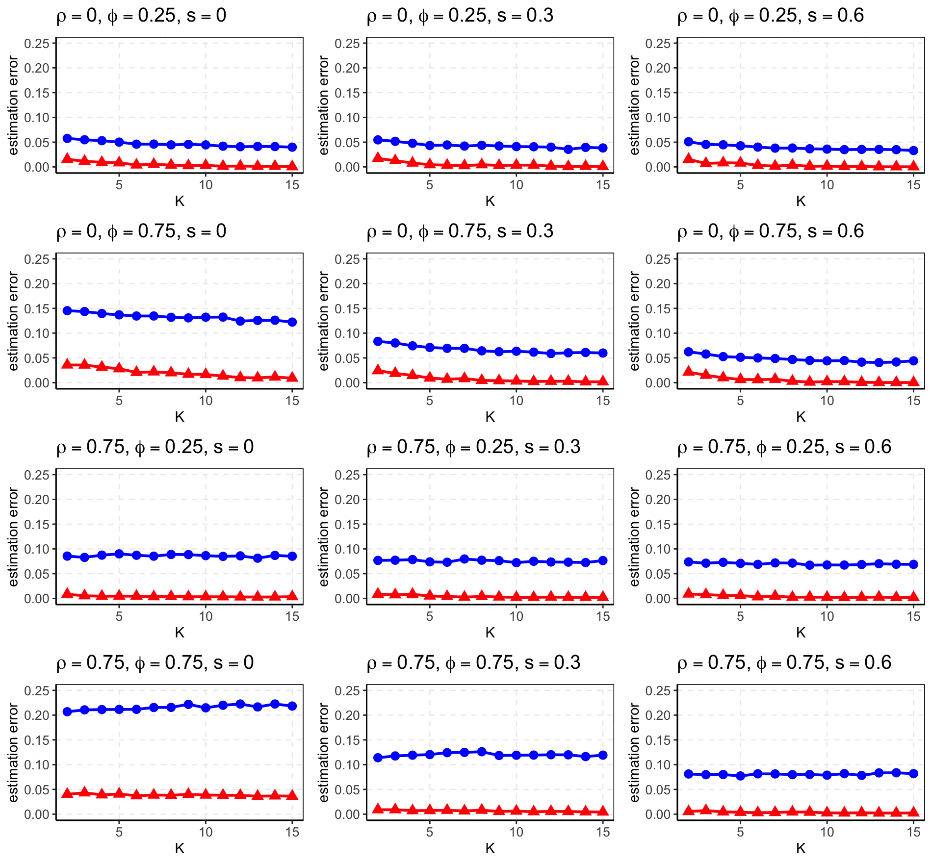Write $d_{\min}=\min_{j\in[m]}d_{j}$ and $\mathbf{Y}=\{\text{vec}(\mathcal{Y}_{1}),\ldots,\text{vec}(\mathcal{Y}_{n})\}^{\mathrm{\scriptscriptstyle\top}}\in\mathbb{R}^{n\times\prod_{j=1}^{m}d_{j}}$ .

First, we determine the lag parameter $K$ . As discussed in Remark 3 of Chang et al. 2023, choosing a larger $K$ makes it more likely that the condition $\textup{rank}(\mathbf{M}_{j})=r$ holds, since more lagged information is incorporated. On the other hand, as shown in Section 5.1 of Chang et al. 2023, an excessively large $K$ may reduce the estimation accuracy of both the number of factors and the factor loading vectors. Balancing these two considerations, Chang et al. 2023 recommend choosing $K\leq 10$ and show through simulations that the estimation performance is robust to the choice of $K$ within a moderate range. Our additional simulations, reported in Figures F4 and F5 in the supplementary material, further support this recommendation. Specifically, the estimation accuracy improves as $K$ increases initially and then stabilizes, with almost no visible change once $K>10$ . Therefore, in practice, we recommend setting $K=10$ .

Second, we introduce how to determine $r$ . When $\xi_{t}$ is specified, for given $\delta_{1}$ and $j\in[m]$ , Chang et al. 2023 employ the eigenvalue-ratio (ER) method to estimate $r$ in the matrix CP-factor model ( $m=2$ ):

\tilde{r}^{(\textup{er})}_{j}(\delta_{1})=\arg\min_{1\leq i\leq\lfloor 0.5d_{\min}\rfloor}\frac{\sigma_{i+1}(\tilde{\mathbf{M}}_{j})+c_{n}}{\sigma_{i}(\tilde{\mathbf{M}}_{j})+c_{n}}\,,\quad j\in[m]\,,

(20)

where $c_{n}\rightarrow 0^{\mathrm{\scriptscriptstyle+}}$ as $n\rightarrow\infty$ , and $\tilde{\mathbf{M}}_{j}$ is the plug-in estimator of $\mathbf{M}_{j}$ specified above (10). Such defined ER method has also been used in Chang et al. 2015; Chang et al. 2018a; Chang et al. 2025 for solving other problems. In practice, we can set $c_{n}=n^{-1}\hat{\sigma}_{0}^{2}$ with $\hat{\sigma}_{0}^{2}=(n\prod_{j=1}^{m}d_{j})^{-1}\|\mathbf{Y}\|_{\rm F}^{2}$ . Notice that $\textup{rank}(\mathbf{M}_{j})=r$ , and Theorem 1 of Chang et al. 2023 implies that $\mathbb{P}\{\tilde{r}^{(\textup{er})}_{j}(\delta_{1})=r\}\to 1$ as $n\to\infty$ under certain regularity conditions for each $j\in[m]$ . For the tensor CP-factor model (1) with more than two modes ( $m>2$ ), to aggregate the information from the estimators $\tilde{r}^{(\textup{er})}_{j}(\delta_{1})$ across all modes, we may consider selecting $\tilde{r}$ as $\max_{j\in[m]}\tilde{r}^{(\textup{er})}_{j}(\delta_{1})$ . However, when the factor loading vectors or the factor processes are highly correlated, the largest eigenvalue of $\tilde{\mathbf{M}}_{j}$ may be inflated relative to the remaining eigenvalues. As pointed out by Brown 1989, this may lead to the so-called “one-factor bias”, under which the conventional ER method tends to favor a one-factor model even when the true number of factors is larger than one. This phenomenon is particularly pronounced when the sample size $n$ is small and is also consistent with the simulation results reported in Table 1 in Section 4. To avoid this issue, we suggest estimating $r$ by $\max_{j\in[m]}\tilde{r}_{j}^{(\log)}(\delta_{1})$ , where

\tilde{r}^{(\text{log})}_{j}(\delta_{1})=\arg\min_{1\leq i\leq\lfloor 0.5d_{\min}\rfloor}\frac{\log\{1+\sigma_{i+1}(\tilde{\mathbf{M}}_{j})\}+c_{n}}{\log\{1+\sigma_{i}(\tilde{\mathbf{M}}_{j})\}+c_{n}}\,,\quad j\in[m]\,,

(21)

with the same setting as in (20). Table 1 in Section 4 shows that the logarithmic eigenvalue-ratio (log-ER) method (21) exhibits better finite-sample performance than the ER method (20). Specifically, when there is a high degree of correlation among factor loading vectors, the ER method tends to underestimate the number of factors, whereas the log-ER method performs stably across all scenarios. Theorem T3 in the supplementary material establishes the consistency of the ER and log-ER estimators. Section D.2 in the supplementary material further examines the robustness of the proposed estimation procedures in Sections 3.1 and 3.2 to misspecification of $r$ .

Next, we consider how to select $\xi_{t}$ . For the special case of the tensor CP-factor model (1) with $m=2$ , Chang et al. 2023 suggest selecting $\xi_{t}$ as the average of the principal components of $\{\text{vec}(\mathcal{Y}_{t})\}_{t=1}^{n}$ . Here, we propose a randomized projection approach to select $\xi_{t}$ , which can be viewed as the extension of the method suggested by Chang et al. 2023. For a prescribed integer $p>1$ , perform PCA on $\mathbf{Y}$ and then obtain the first $p$ principal components, denoted by $\{\tilde{\eta}_{t,1},\ldots,\tilde{\eta}_{t,p}\}_{t=1}^{n}$ . We then randomly generate a set of $p\times p$ orthonormal matrices $\bm{\Omega}^{(1)},\ldots,\bm{\Omega}^{(M)}$ and define $\xi^{(l)}_{t}=p^{-1}\sum_{i=1}^{p}\eta^{(l)}_{t,i}$ with $(\eta^{(l)}_{t,1},\ldots,\eta^{(l)}_{t,p})^{\mathrm{\scriptscriptstyle\top}}=\bm{\Omega}^{(l)}(\tilde{\eta}_{t,1},\ldots,\tilde{\eta}_{t,p})^{\mathrm{\scriptscriptstyle\top}}$ . Our goal is to choose the optimal candidate from $\xi^{(1)}_{t},\ldots,\xi^{(M)}_{t}$ as the final $\xi_{t}$ . For each $l\in[M]$ and a given $\breve{r}\geq r$ , we obtain $\tilde{\mathbf{a}}_{i,j}(l)$ in the same manner as $\tilde{\mathbf{a}}_{i,j}$ defined in Section 3.1 for $i\in[\breve{r}]$ and $j\in[m]$ but with replacing $(\xi_{t},\tilde{r})$ by $(\xi^{(l)}_{t},\breve{r})$ . Our guiding principle is to choose the index $l$ for which the associated estimates $\{\tilde{\mathbf{a}}_{i,j}(l)\}_{i\in[\breve{r}],j\in[m]}$ are most similar to the other estimates $\{\tilde{\mathbf{a}}_{i,j}(\tilde{l})\}_{i\in[\breve{r}],j\in[m],\tilde{l}\neq l}$ . For any $l\in[M]$ , we consider the measure

D(l)=\sum_{\tilde{l}\neq l}\sum_{i=1}^{\breve{r}}I\bigg\{\max_{j\in[m]}\min_{\ell\in[\breve{r}]}[1-|\{\tilde{\mathbf{a}}_{i,j}(l)\}^{\mathrm{\scriptscriptstyle\top}}\tilde{\mathbf{a}}_{\ell,j}(\tilde{l})|^{2}]<\varepsilon\bigg\}\,,

where $\varepsilon>0$ is a prescribed distance threshold. The measure $D(l)$ quantifies the similarity between $\{\tilde{\mathbf{a}}_{i,j}(l)\}_{i\in[\breve{r}],\,j\in[m]}$ and $\{\tilde{\mathbf{a}}_{i,j}(\tilde{l})\}_{i\in[\breve{r}],\,j\in[m]}$ with $\tilde{l}\neq l$ , where larger values of $D(l)$ indicate higher similarity. We then select $\xi_{t}$ as $\xi^{(l^{*})}_{t}$ with $l^{*}=\arg\max_{l\in[M]}D(l)$ . In practice, we set $p=10$ , $\breve{r}=2\tilde{r}^{*}$ , $M=50$ and $\varepsilon=0.1$ , where $\tilde{r}^{*}$ is an initial estimate of $r$ obtained via the log-ER method (21) with $\xi_{t}$ selected using the approach proposed in Chang et al. 2023.

Finally, we determine the threshold levels $\delta_{1}$ and $\{\delta_{2,j}\}_{j=1}^{m}$ . Let $\tilde{v}^{(\textup{log})}_{j}(\delta_{1})$ be the minimal ratio in (21) corresponding to the $j$ -th mode for a given $\delta_{1}$ . We can select $\delta_{1}$ as

\delta_{1}=\arg\min_{0<\delta<0.1\hat{\sigma}_{0}(n^{-1}\sum_{j=1}^{m}\log d_{j})^{1/2}}\frac{1}{m}\sum_{j=1}^{m}\tilde{v}^{(\textup{log})}_{j}(\delta)\,.

Additionally, we suggest setting $\delta_{2,j}=\tilde{C}_{*}\hat{\sigma}_{0}(n^{-1}\log d_{j})^{1/2}$ with some prescribed constant $\tilde{C}_{*}\geq 0$ . Extensive simulation studies demonstrate that the performance of Algorithm 1 introduced in Section 3.2 with such selected $\delta_{2,j}$ is robust with respect to $\tilde{C}_{*}\in[0,1]$ . We therefore recommend setting $\tilde{C}_{*}=1$ in practice.

4 Numerical studies

We generate the observations $\{\mathcal{Y}_{t}\}_{t=1}^{n}$ via the tensor CP-factor model (1). For each $j\in[m]$ , we generate $\mathbf{A}^{*}_{j}=(\mathbf{a}^{*}_{1,j},\ldots,\mathbf{a}^{*}_{r,j})\in\mathbb{R}^{d_{j}\times r}$ with elements drawn independently from the uniform distribution $U(-1,1)$ , subject to the restriction $\text{rank}(\mathbf{A}^{*}_{j})=r$ , and let $\breve{\mathbf{a}}_{1,j}=\mathbf{a}^{*}_{1,j}$ and $\breve{\mathbf{a}}_{i,j}=\mathbf{a}^{*}_{i,j}+\phi\mathbf{a}^{*}_{i-1,j}$ for $2\leq i\leq r$ . For each $i\in[r]$ and $j\in[m]$ , we obtain $\bar{\mathbf{a}}_{i,j}$ based on $\breve{\mathbf{a}}_{i,j}$ by randomly setting its $\lfloor sd_{j}\rfloor$ components to be zero, and let $\mathbf{a}_{i,j}=\bar{\mathbf{a}}_{i,j}/|\bar{\mathbf{a}}_{i,j}|_{2}$ . Here, the parameters $s$ and $\phi$ , respectively, control the sparsity of $\mathbf{a}_{i,j}$ and the correlations among $(\mathbf{a}_{1,j},\ldots,\mathbf{a}_{r,j})$ . We generate $\{f^{*}_{t,i}\}_{t=1}^{n}$ for $i\in[r]$ as $r$ independent AR(1) sequences, i.e. $f^{*}_{t,i}=\beta_{i}f^{*}_{t-1,i}+v_{t,i}$ , where the innovations $v_{t,i}$ are independently drawn from the standard normal distribution $\mathcal{N}(0,1)$ , and let $(f_{t,1},\ldots,f_{t,r})^{\mathrm{\scriptscriptstyle\top}}=\mathbf{J}^{1/2}(f^{*}_{t,1},\ldots,f^{*}_{t,r})^{\mathrm{\scriptscriptstyle\top}}$ , where $\mathbf{J}$ is an $r\times r$ matrix with $[\mathbf{J}]_{i,j}=I(i=j)+\rho I(i\neq j)$ . Here, the parameter $\rho$ governs the correlation among the factor processes. The elements of the error term sequence $\{\mathcal{E}_{t}\}_{t=1}^{n}$ are independently drawn from $\mathcal{N}(0,1)$ . We set $m=2$ (matrix time series), $r=3$ (three factors), $w_{i}=15$ , $d_{j}=20$ , $\beta_{i}=0.85-0.05i$ , $n\in\{400,800\}$ , $s\in\{0,0.3,0.6\}$ , $\phi\in\{0.25,0.75\}$ and $\rho\in\{0,0.75\}$ . We follow the methods described in Section 3.4 to select the tuning parameters involved in our proposed methods.

Table 1 compares the performance of two estimation methods (the ER estimator and the log-ER estimator) introduced in Section 3.4 and the unfolded eigenvalue-ratio (Unfolded-ER) estimator considered in Chen et al. 2026 for estimating $r$ . We can find that log-ER outperforms ER in estimating $r$ across all scenarios, and that, except for the case $(\rho,\phi,s)=(0.75,0.75,0)$ , the performance of log-ER is comparable to that of Unfolded-ER. When $(\rho,\phi,s)=(0.75,0.75,0)$ , both ER and Unfolded-ER tend to underestimate $r$ , whereas log-ER still maintains high accuracy in estimating $r$ .

Table 1: Relative frequency estimates of

\mathbb{P}(\tilde{r}<r)

\mathbb{P}(\tilde{r}=r)

and

\mathbb{P}(\tilde{r}>r)

with

\tilde{r}

determined by the ER estimator (20), the log-ER estimator (21) and the Unfolded-ER estimator based on 2000 repetitions. All numbers reported below are multiplied by 100.

$\rho$	$\phi$	$s$	$n$	log-ER			ER			Unfolded-ER
$\rho$	$\phi$	$s$	$n$	$\mathbb{P}(\tilde{r}<r)$	$\mathbb{P}(\tilde{r}=r)$	$\mathbb{P}(\tilde{r}>r)$	$\mathbb{P}(\tilde{r}<r)$	$\mathbb{P}(\tilde{r}=r)$	$\mathbb{P}(\tilde{r}>r)$	$\mathbb{P}(\tilde{r}<r)$	$\mathbb{P}(\tilde{r}=r)$	$\mathbb{P}(\tilde{r}>r)$
0	0.25	0	400	0.25	99.75	0.00	6.30	93.70	0.00	0.00	100.00	0.00
		0	800	0.65	99.35	0.00	7.55	92.45	0.00	0.00	100.00	0.00
		0.3	400	0.40	99.60	0.00	4.80	95.20	0.00	0.00	100.00	0.00
		0.3	800	0.40	99.60	0.00	6.85	93.15	0.00	0.00	100.00	0.00
		0.6	400	0.10	99.90	0.00	2.80	97.20	0.00	0.00	100.00	0.00
		0.6	800	0.55	99.45	0.00	6.05	93.95	0.00	0.00	100.00	0.00
	0.75	0	400	4.55	95.45	0.00	44.60	55.40	0.00	0.00	100.00	0.00
		0	800	1.60	98.40	0.00	39.05	60.95	0.00	0.00	100.00	0.00
		0.3	400	0.60	99.40	0.00	14.05	85.95	0.00	0.00	100.00	0.00
		0.3	800	0.35	99.65	0.00	11.85	88.15	0.00	0.00	100.00	0.00
		0.6	400	0.10	99.90	0.00	4.25	95.75	0.00	0.00	100.00	0.00
		0.6	800	0.20	99.80	0.00	5.20	94.80	0.00	0.00	100.00	0.00
0.75	0.25	0	400	0.10	99.90	0.00	5.30	94.70	0.00	0.10	99.90	0.00
		0	800	0.00	100.00	0.00	1.25	98.75	0.00	0.00	100.00	0.00
		0.3	400	0.00	100.00	0.00	2.05	97.95	0.00	0.00	100.00	0.00
		0.3	800	0.00	100.00	0.00	0.80	99.20	0.00	0.00	100.00	0.00
		0.6	400	0.15	99.85	0.00	1.75	98.25	0.00	0.05	99.95	0.00
		0.6	800	0.00	100.00	0.00	0.95	99.05	0.00	0.00	100.00	0.00
	0.75	0	400	13.80	86.20	0.00	71.20	28.80	0.00	66.25	33.75	0.00
		0	800	0.55	99.45	0.00	17.50	82.50	0.00	37.90	62.10	0.00
		0.3	400	0.65	99.35	0.00	15.95	84.05	0.00	7.40	92.60	0.00
		0.3	800	0.00	100.00	0.00	2.55	97.45	0.00	0.50	99.50	0.00
		0.6	400	0.15	99.85	0.00	3.45	96.55	0.00	0.50	99.50	0.00
		0.6	800	0.00	100.00	0.00	1.10	98.90	0.00	0.05	99.95	0.00

We also compare the performance of our proposed one-pass initial estimate (Pro.init) introduced in Section 3.1 and iterative estimate (Pro.iter) introduced in Section 3.2 with the composite PCA method (cPCA) and High-Order Projection Estimator (HOPE) proposed by Han et al. 2024b, the methods of Randomized Projection PCA (RP-PCA) and Contemporary Covariance-based Iterative Simultaneous Orthogonalization (CC-ISO) proposed by Chen et al. 2026, and the refined estimate for the matrix CP-factor model (RCP) proposed by Chang et al. 2023. Notice that cPCA, RP-PCA and RCP are one-pass estimates, and HOPE and CC-ISO are iterative estimates. We set the tuning parameter $h=1$ in cPCA and HOPE, as in the simulation studies of Han et al. 2024b, and the tuning parameter $K=10$ in RCP as suggested by Chang et al. 2023. As shown in Section B.1 in the supplementary material, our proposed methods are robust to the selection of $K$ . For each method, the estimation error between the obtained estimates $\{\check{\mathbf{a}}_{i,j}\}_{i\in[\tilde{r}],j\in[m]}$ and the true factor loading vectors $\{\mathbf{a}_{i,j}\}_{i\in[r],j\in[m]}$ is measured by

\psi^{2}(\{\check{\mathbf{a}}_{i,j}\}_{i\in[\tilde{r}],j\in[m]},\{\mathbf{a}_{i,j}\}_{i\in[r],j\in[m]})=\max_{j\in[m]}\max_{\ell\in[r]}\min_{i\in[\tilde{r}]}(1-|\check{\mathbf{a}}_{i,j}^{\mathrm{\scriptscriptstyle\top}}\mathbf{a}_{\ell,j}|^{2})\,,

(22)

where $\tilde{r}$ is the associated estimate of $r$ . For methods without a dedicated procedure for estimating $r$ , we substitute the value obtained from the log-ER estimator when implementing their methods. As shown in Table 2, when $\rho=0$ , Pro.iter performs comparably to CC-ISO and significantly outperforms the other methods. When $\rho=0.75$ , both CC-ISO and HOPE exhibit poor performance, whereas Pro.iter remains effective across all scenarios. Moreover, Pro.init outperforms all other one-pass estimators in all scenarios. Given $\tilde{r}=r$ , we further evaluate the iterative efficiency of Pro.iter against CC-ISO and HOPE. For Pro.iter, we consider three choices of the initialization: Pro.init, cPCA, and RP-PCA. As shown in Figure 1, the estimation errors of Pro.iter converge to nearly zero in very few iterations across different scenarios, irrespective of the initial estimates used. However, HOPE and CC-ISO require more steps for iterative convergence. When $\rho=0.75$ , the estimation errors of HOPE and CC-ISO cannot converge to zero even after a large number of iterations. This suggests that these two methods break down under such scenarios, whereas our iterative algorithm remains effective. Recall that $\rho$ measures the degree of correlation among factors, with larger values corresponding to stronger factor correlations. The simulation results demonstrate that HOPE and CC-ISO perform poorly in scenarios with highly correlated factors. Notice that HOPE proposed by Han et al. 2024b explicitly requires the uncorrelated factor assumption, i.e. $\mathbb{E}(f_{t,i}f_{t-k,j})=0$ for all $i\neq j$ and $k\geq 1$ , while our proposed methods do not rely on this assumption.

Table 2: The averages and standard deviations (in parentheses) of the estimation errors (22) for different methods based on 2000 repetitions. Bold numbers indicate the smallest average estimation error among all competing methods. All numbers reported below are multiplied by 100.

$\rho$	$\phi$	$s$	$n$	Iterative estimates			One-pass estimates
$\rho$	$\phi$	$s$	$n$	Pro.iter	HOPE	CC-ISO	Pro.init	cPCA	RP-PCA	RCP
0	0.25	0	400	0.26 (4.47)	0.67 (7.42)	0.75 (7.67)	4.44 (8.52)	17.01 (17.16)	19.28 (17.99)	31.77 (38.92)
		0	800	0.63 (7.59)	0.78 (8.34)	0.39 (5.52)	2.80 (8.82)	14.40 (16.01)	16.79 (16.27)	27.06 (37.09)
		0.3	400	0.40 (5.87)	0.93 (9.05)	0.47 (6.43)	4.23 (8.86)	14.94 (17.15)	16.54 (17.88)	29.74 (38.40)
		0.3	800	0.36 (5.53)	0.47 (6.23)	0.48 (6.30)	2.24 (6.81)	11.72 (14.86)	13.47 (15.81)	26.22 (37.14)
		0.6	400	0.12 (2.89)	0.82 (8.46)	0.69 (7.64)	3.46 (6.20)	13.61 (17.82)	14.85 (17.92)	28.83 (37.90)
		0.6	800	0.50 (6.66)	0.63 (7.46)	0.48 (6.67)	2.14 (7.65)	9.99 (15.05)	10.98 (15.13)	25.11 (36.79)
	0.75	0	400	1.55 (7.31)	1.99 (7.91)	0.53 (3.88)	12.15 (15.88)	32.07 (10.40)	33.59 (10.33)	52.67 (31.25)
		0	800	0.53 (4.39)	1.35 (6.33)	0.83 (5.01)	5.09 (10.28)	33.49 (10.27)	34.49 (10.27)	54.65 (31.55)
		0.3	400	0.45 (5.50)	0.74 (6.73)	0.54 (5.48)	6.59 (11.90)	25.73 (15.45)	28.57 (14.94)	40.10 (38.10)
		0.3	800	0.27 (4.26)	0.57 (5.52)	0.64 (5.76)	2.92 (7.37)	26.25 (14.52)	30.18 (14.13)	42.32 (39.31)
		0.6	400	0.12 (2.62)	0.72 (7.72)	0.37 (5.10)	4.17 (7.60)	17.99 (17.77)	19.52 (17.66)	31.90 (38.83)
		0.6	800	0.20 (4.13)	0.40 (5.54)	0.30 (4.73)	2.10 (7.01)	15.18 (16.13)	17.47 (16.75)	28.32 (37.64)
0.75	0.25	0	400	0.37 (2.51)	24.74 (37.81)	27.41 (38.74)	8.75 (13.39)	48.35 (14.97)	49.65 (14.48)	22.31 (25.08)
		0	800	0.12 (0.05)	23.64 (37.38)	24.29 (37.29)	4.50 (8.96)	48.54 (14.26)	48.89 (13.65)	21.08 (25.36)
		0.3	400	0.22 (0.11)	27.39 (39.77)	29.57 (40.26)	7.80 (12.18)	49.57 (16.08)	50.56 (15.15)	21.85 (25.60)
		0.3	800	0.09 (0.04)	29.66 (40.68)	29.79 (40.63)	3.58 (7.33)	50.31 (15.64)	51.27 (15.06)	19.13 (23.97)
		0.6	400	0.32 (3.66)	30.52 (41.50)	31.97 (41.82)	6.74 (10.93)	51.31 (18.01)	52.42 (16.77)	20.94 (24.68)
		0.6	800	0.08 (0.03)	32.94 (42.23)	32.56 (41.97)	3.15 (6.75)	51.05 (17.24)	52.10 (16.47)	20.31 (25.42)
	0.75	0	400	4.07 (9.69)	6.57 (15.32)	30.07 (21.34)	21.52 (18.99)	38.28 (8.65)	42.07 (9.09)	27.61 (20.44)
		0	800	0.34 (1.39)	4.02 (14.52)	18.10 (21.57)	10.20 (13.27)	38.59 (9.06)	39.92 (8.32)	23.73 (20.67)
		0.3	400	0.49 (2.52)	13.68 (28.22)	17.83 (30.08)	12.23 (16.41)	44.22 (10.84)	45.84 (10.59)	23.49 (23.76)
		0.3	800	0.12 (0.05)	12.97 (27.65)	14.70 (28.94)	5.03 (8.92)	44.37 (10.81)	45.29 (10.61)	20.89 (23.60)
		0.6	400	0.28 (2.41)	22.73 (37.14)	24.11 (37.76)	8.39 (13.31)	49.42 (14.94)	50.52 (14.37)	22.16 (25.61)
		0.6	800	0.09 (0.04)	25.04 (38.18)	25.42 (38.16)	3.27 (6.39)	50.41 (14.25)	50.68 (13.61)	19.13 (23.68)

Refer to caption — Figure 1: The lineplots for the averages of estimation errors (22) in the first 20 iterative steps based on 2000 repetitions. The sample size $n=400$ . The legend is defined as follows: (i) Pro.iter initialized with Pro.init ( $-$

$\blacksquare$

$-$ ), (ii) Pro.iter initialized with cPCA ( $\color[rgb]{0,1,0}{-\vartriangle-}$ ), (iii) Pro.iter initialized with RP-PCA ( $-\circ-$ ), (iv) HOPE ( $\color[rgb]{1,0,0}{-\blacktriangle-}$ ), and (v) CC-ISO ( $\color[rgb]{0,0,1}{-\bullet-}$ ).

We also evaluate the asymptotic normality (18) and (19) for the iterative estimator $\hat{\mathbf{a}}_{i,j}$ obtained in Algorithm 1 for two choices of $\mathbf{h}$ : (i) $\mathbf{h}_{1}=(1,0,\ldots,0)^{\mathrm{\scriptscriptstyle\top}}$ and (ii) $\mathbf{h}_{2}=(d_{j}^{-1/2},\ldots,d_{j}^{-1/2})^{\mathrm{\scriptscriptstyle\top}}$ . It should be noted that there exists the reflection and permutation indeterminacy between the estimates and the true factor loadings. Here we set $(i,j)=(1,1)$ and impose $z_{1}=\arg\min_{i\in[\tilde{r}]}\{1-|\mathbf{a}_{1,1}^{\mathrm{\scriptscriptstyle\top}}\hat{\mathbf{a}}_{i,1}|^{2}\}$ , thereby eliminating the reflection and permutation indeterminacy between $\hat{\mathbf{a}}_{z_{1},1}$ and $\text{sign}(\mathbf{a}_{1,1}^{\mathrm{\scriptscriptstyle\top}}\hat{\mathbf{a}}_{z_{1},1})\cdot\mathbf{a}_{1,1}$ . We exclude the replications with $\tilde{r}\neq r$ to avoid outliers. Figures 2 and 3 present the histograms of $\{\hat{w}_{z_{1},1}\hat{\tau}_{z_{1},1}^{-1}(\mathbf{h}_{k})\}\sqrt{n}\,\mathbf{h}_{k}^{\mathrm{\scriptscriptstyle\top}}\{\hat{\mathbf{a}}_{z_{1},1}-\text{sign}(\mathbf{a}_{1,1}^{\mathrm{\scriptscriptstyle\top}}\hat{\mathbf{a}}_{z_{1},1})\cdot\mathbf{a}_{1,1}-\hat{\bm{\vartheta}}_{z_{1},1}\}$ for $k\in\{1,2\}$ based on 2000 repetitions, which verify the asymptotic normality of our iterative estimator based on the asymptotic variance estimation $\hat{w}_{z_{1},1}^{-2}\hat{\tau}_{z_{1},1}^{2}(\mathbf{h})$ . Figures F1 and F2 in the supplementary material also verify the asymptotic normality of our iterative estimator based on the asymptotic variance estimation $\hat{w}_{z_{1},1}^{-2}\tilde{\tau}_{z_{1},1}^{2}(\mathbf{h})$ .

We finally evaluate the computational speed and cost of the proposed iterative method initialized with our one-pass estimator. We fix $n=400$ and vary $(d_{1},d_{2})\in\{(20,20),(40,40),$ $(60,60),(80,80)\}$ . Across multiple scenarios, we benchmark the proposed Pro.iter (initialized with Pro.init) against HOPE and CC-ISO in terms of runtime and peak RAM, accounting for both initialization and iterative-phase costs. Figure 4 plots the averages of runtime with standard deviation bands (shaded regions) for the proposed method, HOPE, and CC-ISO across different scenarios, based on 100 replications. Results for peak RAM are similar and can be found in Figure F3 in the supplementary material. When the target tensor is low dimensional, the runtime and peak RAM of Pro.iter are comparable to HOPE and CC-ISO. As dimensionality increases, Pro.iter attains markedly shorter runtime and lower peak RAM usage than HOPE and CC-ISO.

5 Real data analysis: Air pollution data

In this section, we analyze the spatio-temporal structure of air pollution in Beijing using a multi-dimensional representation of the monitoring data. This dataset contains six hourly air-pollution variables ( $\textup{PM}_{2.5},\textup{PM}_{10},\textup{SO}_{2},\textup{NO}_{2},\textup{CO}$ and $\textup{O}_{3}$ ) from 12 nationally controlled air-quality monitoring stations in Beijing, which can be downloaded from https://archive.ics.uci.edu/dataset/501/beijing+multi+site+air+quality+data. The observation period spans from March 1, 2013, to February 28, 2017.

The dataset contains some missing and extreme values, which were handled through interpolation. Since our focus is on the spatio-temporal structure of air-pollution variations, we apply differencing to the hourly pollutant observations for each monitoring site and pollutant type. All series are standardized to remove the impact of different measurement scales. The aforementioned procedures result in a tensor time series $\mathcal{Y}_{t}=(y_{t,\ell_{1},\ell_{2},\ell_{3}})_{12\times 6\times 24}$ for $t\in[1461]$ (i.e. $m=3,d_{1}=12,d_{2}=6,d_{3}=24,n=1461$ ), where $y_{t,\ell_{1},\ell_{2},\ell_{3}}$ records the concentration change of pollutant $\ell_{2}$ at station $\ell_{1}$ during the $\ell_{3}$ -th hour of day $t$ . Figure F6 in the supplementary material shows the time series plots of $\{\mathcal{Y}_{t}\}_{t=1}^{n}$ . This tensor representation enables the exploration of multi-way dependencies in Beijing’s air quality data, revealing how pollution intensity co-varies across space, time, and pollutant dimensions.

We use the tensor CP-factor model (1) to fit $\{\mathcal{Y}_{t}\}_{t=1}^{n}$ , where $\mathbf{a}_{i,j}$ represents the factor loading vector of the $i$ -th factor in the $j$ -th mode. To estimate the factor loading vectors based on our proposed method, we set the tuning parameters following Section 3.4. Using the proposed log-ER method, we obtain $\tilde{r}=2$ , indicating the presence of two latent factors. Initialized with the one-pass estimator introduced in Section 3.1, the proposed iterative estimator in Algorithm 1 converges successfully.

Table 3 presents the estimations of the factor loadings $\mathbf{a}_{i,2}\in\mathbb{R}^{6}$ based on Pro.iter, which reveal two main patterns of pollutant variation. The first loading vector ( $i=1$ ) has a very high value for O₃ (0.953) but small values for other pollutants, indicating that this factor mainly reflects changes in ozone concentration, which vary differently from other pollutants. The second loading vector ( $i=2$ ) has positive values for PM_2.5, PM₁₀, SO₂, NO₂, and CO, suggesting a common pollution pattern where several pollutants increase or decrease together. Therefore, we refer to the first estimated factor as the ozone-related factor, which mainly captures variations driven by O₃, and the second as the general pollution factor, representing the joint fluctuation of multiple pollutants.

Table 3: Estimations of the loading vectors

\mathbf{a}_{i,2}\in\mathbb{R}^{6}

for the pollution-variable mode based on Pro.iter. Standard errors reported in parentheses are calculated based on the asymptotic variance estimation

\hat{w}_{i,j}^{-2}\hat{\tau}_{i,j}^{2}(\mathbf{h})

. ^∗, ^∗∗, and ^∗∗∗ indicate significance at the levels 5%, 1%, and 1‰, respectively, based on two-sided

t

-tests.

Pollutant	$i=1$	$i=2$
PM_2.5	0.008 (0.015)	0.659^∗∗∗ (0.035)
PM₁₀	$-$ 0.021 (0.013)	0.430^∗∗∗ (0.025)
SO₂	0.049^∗∗ (0.017)	0.304^∗∗∗ (0.036)
NO₂	$-$ 0.236^∗∗∗ (0.016)	0.289^∗∗∗ (0.053)
CO	0.182^∗∗∗ (0.012)	0.452^∗∗∗ (0.031)
O₃	0.953^∗∗∗ (0.002)	0.009 (0.083)

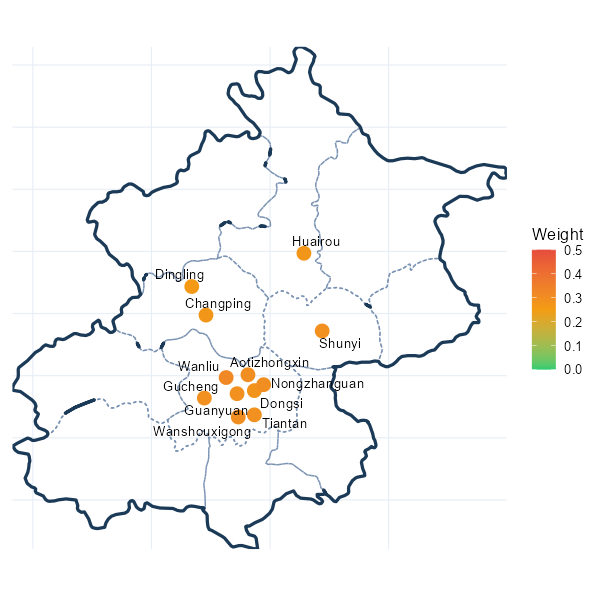
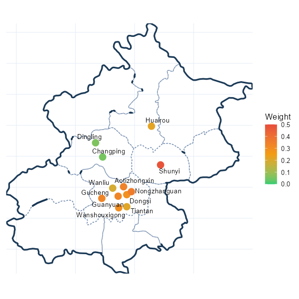
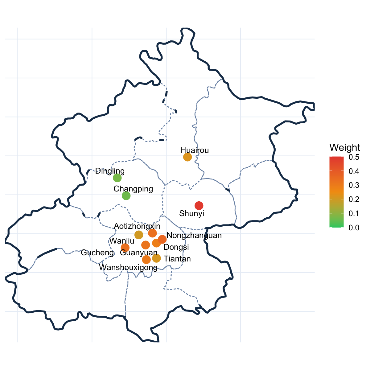
Figure 5 illustrates the estimations of the factor loadings $\mathbf{a}_{i,1}\in\mathbb{R}^{12}$ based on Pro.iter for the monitoring-station mode. Figure 5(a) shows the factor loadings of the ozone-related factor to be nearly uniform across stations, indicating the dominance of regional photochemistry and synoptic meteorology rather than local emissions. Figure 5(b) reveals pronounced spatial heterogeneity for the general pollution factor: Dingling and Changping (northern mountains) have small loadings due to sparse population, limited sources, and effective ventilation, whereas Shunyi (eastern plain, downwind of the urban core and influenced by airport, traffic, and industry) exhibits the largest loading, consistent with higher emissions and advective transport. Moreover, as reported in Table T3 in the supplementary material, all estimated loadings based on Pro.iter for the ozone-related factor are statistically significant, while for the general pollution factor, all estimated loadings are statistically significant except those corresponding to Dingling and Changping. These results provide additional inferential support for the corresponding spatial interpretation.

Figure 6 illustrates the estimations of the factor loadings $\mathbf{a}_{i,3}\in\mathbb{R}^{24}$ based on Pro.iter for the diurnal mode. The loading vector of the ozone-related factor rises after sunrise, peaks around 13:00–14:00, and turns negative at night, tracking the canonical photochemical cycle of daytime production and nocturnal loss via deposition (Li et al. 2015). By contrast, the general pollution factor is distinctly bimodal—minimal before dawn, a first peak near 10:00–11:00, and a higher evening peak (around 19:00–20:00). This bimodal profile accords with established diurnal emission and mixing cycles: a morning peak from traffic and industrial start-up, and a higher evening peak from rush-hour emissions combined with boundary-layer stabilization that suppresses dispersion. Analogous morning–evening bimodality for urban aerosols (e.g., $\textup{PM}_{2.5}$ and $\textup{PM}_{10}$ in Beijing) is well documented (Liu et al. 2015). Overall, the two factors capture complementary diurnal dynamics—one driven by photochemical reactions (ozone-related) and the other by human emission activities (general pollution).

Figure 7 presents the time series of the two estimated latent factors based on Pro.iter; see Section C in the supplementary material for details on the factor estimation procedure. Figure 7(a) shows the ozone-related factor, which exhibits a distinct seasonal cycle with higher values in summer and lower values in winter. This pattern aligns with ozone’s photochemical formation mechanism, which is strongly dependent on solar radiation and temperature. Figure 7(b) depicts the general pollution factor, displaying the opposite seasonal pattern—higher values in cold seasons and lower values in warm seasons. This arises because cold months see increased coal/fuel combustion for heating (releasing more fine particles and gases) and stable atmospheric conditions; in contrast, summer features stronger air movement, higher wind speeds, and frequent rainfall, which stir, disperse, and scavenge pollutants to improve air quality.

Overall, by representing the multi-site, multi-pollutant, and hourly observations as a tensor time series, the proposed CP-factor estimation method successfully identifies two dominant latent components that capture distinct physical mechanisms underlying Beijing’s air pollution. The ozone-related factor reflects photochemical processes, whereas the general pollution factor represents anthropogenic emission activities. Together, these two factors provide a concise and interpretable characterization of the complementary seasonal dynamics of photochemically and emission-driven pollution in Beijing. Section B.2 in the supplementary material reports the results of the real data analysis based on the other three methods (Pro.init, HOPE, and CC-ISO). The findings suggest that the estimates of Pro.iter are more interpretable and more consistent with well-established pollution mechanisms than those produced by Pro.init, HOPE, and CC-ISO. To assess the reliability of the above empirical results, we also show in Section B.2 in the supplementary material that these results remain essentially unchanged when using the winsorized data, indicating the robustness of our conclusions.

Section B.3 in the supplementary material provides another real data analysis for financial data. It is well known that financial data exhibit strong cross-sectional dependence, and often involve highly correlated latent factors. Table T6 in the supplementary material reports the average forecasting errors for financial returns based on different methods. It can be observed that the tensor CP-factor methods without uncorrelated factor assumption consistently outperform the methods that rely on this assumption, which provides further evidence for the applicability of our proposed methods in practice.

6 Theoretical analysis

6.1 Assumptions

We first present some technical assumptions for our theoretical analysis. Assumptions 2–6 are imposed to guarantee the consistency of the one-pass estimator introduced in Section 3.1. Given a general consistent initial estimator, Assumptions 2–4 and 7 are required to establish the theoretical guarantees for the associated iterative estimator introduced in Section 3.2.

Assumption 2.

There exist universal constants $C_{1}>1$ , $C_{2}>0$ , and $c_{1}\in(0,2]$ such that $\max_{i\in[r]}\max_{t\in[n]}\mathbb{P}(|f_{t,i}|>x)\leq C_{1}\exp(-C_{2}x^{c_{1}})$ , $\max_{j\in[m]}\max_{p_{j}\in[d_{j}]}\max_{t\in[n]}\mathbb{P}(|[\mathcal{E}_{t}]_{p_{1},\ldots,p_{m}}|>x)\leq C_{1}\exp(-C_{2}x^{c_{1}})$ , and $\max_{t\in[n]}\mathbb{P}(|\xi_{t}|>x)\leq C_{1}\exp(-C_{2}x^{c_{1}})$ for any $x>0$ . There also exists a universal constant $C_{3}>0$ such that $w_{1}\geq\cdots\geq w_{r}\geq C_{3}$ .

Assumption 3.

Define the $\alpha$ -mixing coefficients associated with the factors and error processes $\{f_{t,1},\ldots,f_{t,r},\mathcal{E}_{t}\}_{t\geq 1}$ as

\alpha(k)=\sup_{t}\sup_{A\in\mathcal{F}_{-\infty}^{t},\,B\in\mathcal{F}_{t+k}^{\infty}}|\mathbb{P}(A\cap B)-\mathbb{P}(A)\mathbb{P}(B)|\,,~~~k\geq 1\,,

where $\mathcal{F}_{t_{1}}^{t_{2}}$ is the $\sigma$ -field generated by $\{f_{t,1},\ldots,f_{t,r},\mathcal{E}_{t}\}_{t=t_{1}}^{t_{2}}$ . There exist some universal constants $C_{4}>1$ , $C_{5}>0$ and $c_{2}\in(0,1]$ such that $\alpha(k)\leq C_{4}\exp(-C_{5}k^{c_{2}})$ for any $k\geq 1$ .

Assumption 4.

There exists a universal constant $C_{6}>1$ such that $C_{6}^{-1}\leq\sigma_{r}(\mathbf{A}_{j})\leq\sigma_{1}(\mathbf{A}_{j})\leq C_{6}$ for any $j\in[m]$ . It holds that $\max_{i\in[r]}|\mathbf{a}_{i,j}|_{0}\leq s_{j}$ for any $j\in[m]$ .

As pointed out in Chang et al. 2023; Chang et al. 2024a, Assumptions 2 and 3 are standard in the literature on high-dimensional data analysis, which are satisfied for a wide range of time series models. These assumptions ensure exponential-type upper bounds for the tail probabilities of the statistics concerned. Assumption 2 focuses on the cases where all the factors, idiosyncratic errors, and the linear combination $\xi_{t}$ have exponentially decaying tails. Assumption 3 is a standard $\alpha$ -mixing condition allowing the data to be serially dependent but not necessarily stationary. As shown in (4), our procedure is based on lag- $k$ auto-covariances averaged over the sampling periods, rather than on a fixed stationary auto-covariance structure. Therefore, the factor process need not be stationary where $\mathbb{E}(f_{t,i}^{2})$ is allowed to vary with $t$ . Assumption 4 can accommodate both sparse and dense loadings within a unified formulation. For example, if $s_{j}\ll d_{j}$ , Assumption 4 corresponds to the sparse case; if $s_{j}=d_{j}$ , it covers the dense case. Sparse loadings arise naturally in several important settings in the recent factor model literature (Uematsu and Yamagata 2022). Properly handling the sparsity via thresholding can improve estimation efficiency. We only require that $\sigma_{1}(\mathbf{A}_{j}),\ldots,\sigma_{r}(\mathbf{A}_{j})$ are uniformly bounded away from $0$ and $\infty$ for $j\in[m]$ , which is weaker than the requirement $\max_{j\in[m]}\|\mathbf{A}_{j}^{\mathrm{\scriptscriptstyle\top}}\mathbf{A}_{j}-\mathbf{I}_{r}\|_{2}<1$ imposed in Han et al. 2024b and Chen et al. 2026.

Assumption 5.

Define $\underaccent{\bar}{\sigma}_{\xi}^{2}=\min_{i\in[r],j\in[m]}\sigma_{i}(\mathbf{M}_{j})$ and $\bar{\sigma}_{\xi}^{2}=\max_{i\in[r],j\in[m]}\sigma_{i}(\mathbf{M}_{j})$ . Assume that $\underaccent{\bar}{\sigma}_{\xi}\geq C_{7}$ for some universal constant $C_{7}>0$ and $n^{-1/2}\bar{\sigma}_{\xi}w_{1}\ll\underaccent{\bar}{\sigma}_{\xi}^{2}$ .

We can regard $\xi_{t}$ as a projection of $\text{vec}(\mathcal{Y}_{t})$ to a lower dimension. Certainly, we expect that the projection can retain the signal of the factor process, which is guaranteed by Assumption 5. Specifically, by Theorem 7 of Horn et al. 2026, we have

\underaccent{\bar}{\sigma}_{\xi}^{2}\geq\bigg(\min_{i\in[r]}\sum_{k=1}^{K}|g_{k,i,\xi}|^{2}\bigg)\bigg\{\min_{j\in[m]}\frac{\sigma_{r}^{2}(\mathbf{A}_{j})\sigma_{r}^{2}(\mathbf{B}_{j})}{\sigma_{1}^{2}(\mathbf{A}_{j})}\bigg\}\,.

Therefore, for each $i\in[r]$ , if there exists some $k\in[K]$ such that $|g_{k,i,\xi}|$ is bounded away from $0$ , then it follows from Assumption 4 that $\underaccent{\bar}{\sigma}_{\xi}$ is bounded away from $0$ . According to the definition of $\mathbf{M}_{j}$ , we have $\underaccent{\bar}{\sigma}_{\xi}\lesssim\max_{k\in[K],i\in[r]}|g_{k,i,\xi}|\lesssim\bar{\sigma}_{\xi}\lesssim w_{1}$ . If $w_{1},\ldots,w_{r}$ are fixed constants, Assumption 5 holds when both $\bar{\sigma}_{\xi}$ and $\underaccent{\bar}{\sigma}_{\xi}$ are uniformly bounded away from $0$ and $\infty$ . For the toy example mentioned in Section 2 with $\beta\neq 0$ , if we select $\xi_{t}=(\prod_{j=1}^{m}d_{j})^{-1}\sum_{h_{1}=1}^{d_{1}}\cdots\sum_{h_{m}=1}^{d_{m}}[\mathcal{Y}_{t}]_{h_{1},\ldots,h_{m}}$ , then $\bar{\sigma}_{\xi}\asymp\underaccent{\bar}{\sigma}_{\xi}\asymp w_{1}\asymp(\prod_{j=1}^{m}d_{j})^{1/2}$ provided that $|(n-k)^{-1}\sum_{t=k+1}^{n}\mathbb{E}[\{f_{t}-\mathbb{E}(\bar{f})\}\{f_{t-k}-\mathbb{E}(\bar{f})\}]|$ with $\bar{f}=n^{-1}\sum_{t=1}^{n}f_{t}$ is uniformly bounded away from $0$ and $\infty$ , which implies that Assumption 5 holds automatically. For more general scenarios, as long as $\xi_{t}$ is properly selected, it is expected that $\underaccent{\bar}{\sigma}_{\xi}\asymp w_{r}$ and $\bar{\sigma}_{\xi}\asymp w_{1}$ . Then, Assumption 5 will hold when $w_{1}^{2}\ll w_{r}^{2}\sqrt{n}$ , which is a requirement on the relative strength of the factors. A similar condition also appears in Theorem 2 of Han et al. 2024b.

Assumption 6.

All the eigenvalues $\bar{\lambda}_{1},\ldots,\bar{\lambda}_{r}$ in (7) are uniformly bounded away from $0$ and $\infty$ . Moreover, $\min_{i\neq\ell}|\bar{\lambda}_{i}-\bar{\lambda}_{\ell}|\geq C_{8}$ and $\min_{i\in[r]}|g_{2,i,\xi}|\geq C_{8}\underaccent{\bar}{\sigma}_{\xi}$ for some universal constant $C_{8}>0$ , where $g_{2,i,\xi}$ is defined in (5).

To identify the $r$ eigenvectors of $\mathbf{K}_{1,2,j}$ defined in (6) corresponding to its $r$ nonzero eigenvalues, it is crucial that these eigenvalues are distinct. This is a typical assumption in the literature on eigen-analysis; see also Condition 5 in Chang et al. 2023.

Assumption 7.

For any deterministic vector $\bm{\beta}\in\mathbb{R}^{\prod_{j=1}^{m}d_{j}}$ , it holds that

\max_{t\in[n]}\mathbb{P}\{|\bm{\beta}^{\mathrm{\scriptscriptstyle\top}}{\rm vec}(\mathcal{E}_{t})|>x|\bm{\beta}|_{2}\}\leq C_{1}\exp(-C_{2}x^{c_{1}})

for any $x>0$ , where $C_{1}$ , $C_{2}$ , and $c_{1}$ are the same constants as those in Assumption 2.

Assumption 7 provides a tail bound for any linear combination of the idiosyncratic error tensor. It allows for cross-sectional dependence among the errors. This assumption can hold under very general scenarios, e.g., when $\textup{vec}(\mathcal{E}_{t})$ follows a multivariate Gaussian distribution with a covariance matrix bounded in spectral norm; see also Assumption 1 in Han et al. 2024b.

6.2 Theoretical guarantees of the proposed methods

Let $D_{n}=\prod_{j=1}^{m}d_{j}$ and $S_{n}=\prod_{j=1}^{m}s_{j}$ , and further define

\Pi_{n}=\frac{\bar{\sigma}_{\xi}}{\underaccent{\bar}{\sigma}_{\xi}^{2}}\bigg(\frac{S_{n}\log D_{n}}{n}\bigg)^{1/2}\,.

Set the threshold level $\delta_{1}=C_{*}(n^{-1}\log D_{n})^{1/2}$ in (8) for some constant $C_{*}>0$ . Theorem 1 shows the consistency (up to the reflection and permutation indeterminacy) of the one-pass estimator $\{\tilde{\mathbf{a}}_{i,j}\}_{i\in[\tilde{r}],j\in[m]}$ introduced in Section 3.1.

Theorem 1.

Under Assumptions 1–6, if $\Pi_{n}\ll 1$ and $\tilde{r}=r$ , there exists a permutation of $[r]$ , denoted by $\{z_{1},\ldots,z_{r}\}$ , such that

|\tilde{\mathbf{a}}_{z_{i},j}-\tilde{\kappa}_{i,j}\mathbf{a}_{i,j}|_{2}=\underaccent{\bar}{\sigma}_{\xi}\,\bar{\sigma}_{\xi}^{-1}\,O_{\rm p}(\Pi_{n})

for any $i\in[r]$ and $j\in[m]$ with some constants $\tilde{\kappa}_{i,j}\in\{-1,1\}$ , provided that $\log D_{n}\ll n^{c}$ for some constant $c\in(0,1)$ depending only on $c_{1}$ and $c_{2}$ specified in Assumptions 2 and 3.

In Algorithm 1, the estimated factor series $\{\check{f}_{t,i}^{(\textit{v},j)}\}_{t=1}^{n}$ can be regarded as linear combinations of $\{\text{vec}(\mathcal{Y}_{t})\}_{t=1}^{n}$ with some plug-in estimators of the coefficients $(\mathbf{a}_{i,m}^{\mathrm{\scriptscriptstyle+}}\otimes\cdots\otimes\mathbf{a}_{i,1}^{\mathrm{\scriptscriptstyle+}})$ , where $(\mathbf{a}_{1,j}^{\mathrm{\scriptscriptstyle+}},\ldots,\mathbf{a}_{r,j}^{\mathrm{\scriptscriptstyle+}})^{\mathrm{\scriptscriptstyle\top}}=(\mathbf{A}_{j}^{\mathrm{\scriptscriptstyle\top}}\mathbf{A}_{j})^{-1}{\mathbf{A}}_{j}^{\mathrm{\scriptscriptstyle\top}}$ . To study the statistical error of the iterative estimator, we define the oracle linear combinations as $\xi_{t,i}=(\mathbf{a}_{i,m}^{\mathrm{\scriptscriptstyle+}}\otimes\cdots\otimes\mathbf{a}_{i,1}^{\mathrm{\scriptscriptstyle+}})^{\mathrm{\scriptscriptstyle\top}}\text{vec}(\mathcal{Y}_{t})=w_{i}f_{t,i}+(\mathbf{a}_{i,m}^{\mathrm{\scriptscriptstyle+}}\otimes\cdots\otimes\mathbf{a}_{i,1}^{\mathrm{\scriptscriptstyle+}})^{\mathrm{\scriptscriptstyle\top}}\text{vec}(\mathcal{E}_{t})$ , and write

\xi_{t,i}^{\textup{s}}=\bigg[\frac{1}{n}\sum_{s=1}^{n}\mathbb{E}\{(\xi_{s,i}-\bar{\xi}_{i})^{2}\}\bigg]^{-1/2}(\xi_{t,i}-\bar{\xi}_{i})

with $\bar{\xi}_{i}=n^{-1}\sum_{t=1}^{n}\xi_{t,i}$ . If $r=1$ , let $\xi_{t,i}^{\textup{sp}}=\xi_{t,i}^{\textup{s}}$ for $t\in[n]$ and $i\in[r]$ . If $r\geq 2$ , let $\bm{\xi}_{i}^{\textup{s}}=(\xi_{1,i}^{\textup{s}},\ldots,\xi_{n-1,i}^{\textup{s}})^{\mathrm{\scriptscriptstyle\top}}$ , and $\mathbf{F}_{\xi,\scalebox{1}{\text{-}}i}^{\textup{s}}$ be a $(n-1)\times(r-1)$ matrix of which the columns are composed of $(\xi_{2,\ell}^{\textup{s}},\ldots,\xi_{n,\ell}^{\textup{s}})^{\mathrm{\scriptscriptstyle\top}}$ for $\ell\neq i$ . Then, following the double projection step, we define

(\xi_{1,i}^{\textup{sp}},\ldots,\xi_{n-1,i}^{\textup{sp}})^{\mathrm{\scriptscriptstyle\top}}=\bm{\xi}_{i}^{\textup{s}}-\mathbf{F}_{\xi,\scalebox{1}{\text{-}}i}^{\textup{s}}[\mathbb{E}\{(\mathbf{F}_{\xi,\scalebox{1}{\text{-}}i}^{\textup{s}})^{\mathrm{\scriptscriptstyle\top}}\mathbf{F}_{\xi,\scalebox{1}{\text{-}}i}^{\textup{s}}\}]^{-1}\mathbb{E}\{(\mathbf{F}_{\xi,\scalebox{1}{\text{-}}i}^{\textup{s}})^{\mathrm{\scriptscriptstyle\top}}\bm{\xi}_{i}^{\textup{s}}\}\,.

(23)

Let $\bar{\bm{\varphi}}_{i}=(\bar{\varphi}_{i,1},\ldots,\bar{\varphi}_{i,r})^{\mathrm{\scriptscriptstyle\top}}$ be the $r$ -dimensional vector with the $i$ -th entry equal to 1, while the remaining $r-1$ entries form the vector $-[\mathbb{E}\{(\mathbf{F}_{\xi,\scalebox{1}{\text{-}}i}^{\textup{s}})^{\mathrm{\scriptscriptstyle\top}}\mathbf{F}_{\xi,\scalebox{1}{\text{-}}i}^{\textup{s}}\}]^{-1}\mathbb{E}\{(\mathbf{F}_{\xi,\scalebox{1}{\text{-}}i}^{\textup{s}})^{\mathrm{\scriptscriptstyle\top}}\bm{\xi}_{i}^{\textup{s}}\}$ . Then, $\xi_{t,i}^{\textup{sp}}=\xi_{t,i}^{\textup{s}}+\sum_{\ell\neq i}\bar{\varphi}_{i,\ell}\xi_{t+1,\ell}^{\textup{s}}$ for $t\in[n-1]$ .

Set the threshold levels $\delta_{2,j}=\tilde{C}_{*}(n^{-1}\log d_{j})^{1/2}$ for $j\in[m]$ in Algorithm 1 with some sufficiently large constant $\tilde{C}_{*}>0$ . Write

\Phi_{n,j}=\frac{1}{w_{r}}\sqrt{\frac{s_{j}\log d_{j}}{n}}~~\textrm{and}~~\bm{\Upsilon}_{k}=(\Upsilon_{k,i,\ell})_{r\times r}\,,

where $\Upsilon_{k,i,\ell}=(n-k)^{-1}\sum_{t=k+1}^{n}\mathbb{E}\{(f_{t,i}-\bar{f}_{i})(f_{t-k,\ell}-\bar{f}_{\ell})\}$ for $i,\ell\in[r]$ and $k\in\{0,1\}$ . Let

\begin{split}&\gamma_{\max}=\max_{i\neq\ell}|\Upsilon_{1,i,\ell}|\,,~~\sigma_{f_{i},\xi_{i}}=\mathbb{E}\bigg\{\frac{1}{n-1}\sum_{t=2}^{n}(f_{t,i}-\bar{f}_{i})\xi_{t-1,i}^{\textup{sp}}\bigg\}\,,\\ &~~~~~~\textup{and}~~L_{n}=\bigg(\frac{\sum_{j=1}^{m}d_{j}\log d_{j}}{n}\bigg)^{1/2}+\frac{(\sum_{j=1}^{m}d_{j})^{1/\tilde{c}}}{n}\,,\end{split}

(24)

where $\tilde{c}^{-1}=1+2c_{1}^{-1}+c_{2}^{-1}$ for $c_{1}$ and $c_{2}$ in Assumptions 2 and 3. Theorem 2 gives the convergence rate of the iterative estimator obtained by Algorithm 1.

Theorem 2.

Let Assumptions 1–4 and 7 hold. Assume that $\tilde{r}=r$ and the initial estimates in Algorithm 1 satisfy $\max_{i\in[r],j\in[m]}w_{r}^{-1}w_{1}|\tilde{\mathbf{a}}_{z_{i},j}^{(0)}-\tilde{\kappa}_{i,j}\mathbf{a}_{i,j}|_{2}=o_{\rm p}(1)$ for some permutation $\{z_{1},\ldots,z_{r}\}$ of $[r]$ and some constants $\tilde{\kappa}_{i,j}\in\{-1,1\}$ . If $D_{n}\rightarrow\infty$ as $n\rightarrow\infty$ , $C_{9}^{-1}\leq\sigma_{r}(\bm{\Upsilon}_{0})\leq\sigma_{1}(\bm{\Upsilon}_{0})\leq C_{9}$ for some universal constant $C_{9}>1$ ,

\frac{w_{1}}{w_{r}^{2}}\bigg(\frac{\gamma_{\max}}{w_{r}}+\frac{1}{w_{r}\sqrt{n}}+L_{n}\bigg)\ll 1~~\text{and}~~|\sigma_{f_{i},\xi_{i}}|\geq C_{9}^{-1}

(25)

for all $i\in[r]$ , then we have

\max_{i\in[r],j\in[m]}|\hat{\mathbf{a}}_{z_{i},j}-\kappa_{i,j}\mathbf{a}_{i,j}|_{2}=O_{\rm p}\bigg(\max_{j\in[m]}\Phi_{n,j}+\frac{\gamma_{\max}}{w_{r}^{2}}\bigg)\,

for some constants $\kappa_{i,j}\in\{-1,1\}$ , provided that the number of iterations satisfies $\textit{v}_{\max}\gtrsim-\log(\max_{j\in[m]}\Phi_{n,j}+\gamma_{\max}w_{r}^{-2})$ and $\max_{j\in[m]}\log d_{j}\ll n^{c}$ for some constant $c\in(0,1)$ depending only on $c_{1}$ and $c_{2}$ specified in Assumptions 2 and 3.

The requirement on the convergence rate of $\{\tilde{\mathbf{a}}_{i,j}^{(0)}\}_{i\in[\tilde{r}],j\in[m]}$ can be easily satisfied if taking the one-pass estimator introduced in Section 3.1 as the initial estimator of Algorithm 1. As discussed below Assumption 5, when the initial linear combination is properly selected, it is expected that $\underaccent{\bar}{\sigma}_{\xi}\asymp w_{r}$ and $\bar{\sigma}_{\xi}\asymp w_{1}$ . Theorem 1 implies that the convergence rate of the one-pass estimator satisfies this requirement automatically. The first part of condition (25) is mainly to control the plug-in error of $\{\tilde{\mathbf{a}}^{(\textit{v})}_{i,j}\}_{i\in[\tilde{r}],j\in[m]}$ in the iterations. The requirement $w_{1}w_{r}^{-2}n^{-1}(\sum_{j=1}^{m}d_{j})^{1/\tilde{c}}\ll 1$ originates from the serial dependence of the error process $\{\mathcal{E}_{t}\}_{t\geq 1}$ , and is unnecessary if $\{\mathcal{E}_{t}\}_{t\geq 1}$ are serially independent sub-Gaussian tensors, and are also independent of the factor process $\{\mathbf{f}_{t}\}_{t\geq 1}$ . The second part of condition (25) is similar to Assumption 5, which requires the lag-one cross-correlation between $\{\xi_{t,i}^{\textup{sp}}\}_{t=1}^{n}$ and $\{f_{t,i}\}_{t=1}^{n}$ to be non-vanishing. The convergence rate of the iterative estimator includes two parts. The first part depends on $\Phi_{n,j}$ , which is a typical rate under sparsity. The second part depends on the lag-one cross-correlations of the factors $\gamma_{\max}$ and the factor strength $w_{r}$ , which is mainly from the estimation error of the factors when we decorrelate them in the double projection step. Under Assumption 5, we can show that $\underaccent{\bar}{\sigma}_{\xi}\lesssim w_{r}$ . When $\mathbb{E}(f_{t,i})=0$ for all $t,i$ and $\mathbb{E}(f_{t,i}f_{t-k,j})=0$ for all $i\neq j,k\geq 1$ as assumed in Han et al. 2024b, we have $\gamma_{\max}=O(n^{-1})$ and the convergence rate in Theorem 2 can be simplified as $O_{\rm p}(\max_{j\in[m]}\Phi_{n,j})$ , which implies the iterative estimator in this scenario is more accurate in comparison to the one-pass estimator introduced in Section 3.1.

Let $\bar{\mathbf{e}}_{i,j}=n^{-1}\sum_{t=1}^{n}\mathbf{e}_{t,i,j}$ with $\mathbf{e}_{t,i,j}$ defined in (11). With $\xi_{t,i}^{\textup{s}}$ defined above (23), write

\begin{split}\tilde{\bm{\Sigma}}_{\mathbf{e}_{\ell,j},\xi_{i}}(1)&=\frac{1}{n-1}\sum_{t=2}^{n}(\mathbf{e}_{t,\ell,j}-\bar{\mathbf{e}}_{\ell,j})\xi_{t-1,i}^{\textup{s}}\,,\\ \tilde{\bm{\Sigma}}_{\mathbf{e}_{\ell,j},\xi_{i}}(0)&=\frac{1}{n-1}\sum_{t=2}^{n}[(\mathbf{e}_{t,\ell,j}-\bar{\mathbf{e}}_{\ell,j})\xi_{t,i}^{\textup{s}}-\mathbb{E}\{(\mathbf{e}_{t,\ell,j}-\bar{\mathbf{e}}_{\ell,j})\xi_{t,i}^{\textup{s}}\}]\end{split}

(26)

for $j\in[m]$ and any $i,\ell\in[r]$ . Theorem 3 provides a limiting representation for the iterative estimator $\hat{\mathbf{a}}_{i,j}$ .

Theorem 3.

Let $\mathbf{h}\in\mathbb{R}^{d_{j}}$ be any non-random vector satisfying $|\mathbf{h}|_{2}=1$ , and the conditions in Theorem 2 hold. For any $i\in[r]$ and $j\in[m]$ , it holds that

	$\displaystyle\mathbf{h}^{\mathrm{\scriptscriptstyle\top}}(\hat{\mathbf{a}}_{z_{i},j}$	$\displaystyle-\kappa_{i,j}\mathbf{a}_{i,j}-\hat{\bm{\vartheta}}_{z_{i},j})$
	$\displaystyle=\,$	$\displaystyle\frac{\kappa_{i,j}}{w_{i}\sigma_{f_{i},\xi_{i}}}\mathbf{h}^{\mathrm{\scriptscriptstyle\top}}(\mathbf{I}_{d_{j}}-\mathbf{a}_{{i},j}\mathbf{a}_{{i},j}^{\mathrm{\scriptscriptstyle\top}})\bigg\{\tilde{\bm{\Sigma}}_{\mathbf{e}_{i,j},\xi_{i}}(1)+\sum_{\ell\neq i}\bar{\varphi}_{i,\ell}\tilde{\bm{\Sigma}}_{\mathbf{e}_{i,j},\xi_{\ell}}(0)\bigg\}$
		$\displaystyle+O_{\rm p}\bigg(\frac{\gamma_{\max}}{w_{i}w_{r}}+\frac{1}{\sqrt{n}w_{i}w_{r}}+\frac{w_{1}}{w_{i}w_{r}}L_{n}\max_{j\in[m]}\Phi_{n,j}\bigg)+o_{\rm p}\bigg(\frac{1}{w_{i}\sqrt{n}}\bigg)\,,$

where $z_{i}$ and $\kappa_{i,j}$ are specified in Theorem 2, and $\sigma_{f_{i},\xi_{i}}$ and $\bar{\varphi}_{i,\ell}$ are defined, respectively, in (24) and below (23). Furthermore, if

\lim_{n\rightarrow\infty}{\rm Var}\bigg[\frac{\sqrt{n}}{\sigma_{f_{i},\xi_{i}}}\mathbf{h}^{\mathrm{\scriptscriptstyle\top}}(\mathbf{I}_{d_{j}}-\mathbf{a}_{i,j}\mathbf{a}_{i,j}^{\mathrm{\scriptscriptstyle\top}})\bigg\{\tilde{\bm{\Sigma}}_{\mathbf{e}_{i,j},\xi_{i}}(1)+\sum_{\ell\neq i}\bar{\varphi}_{i,\ell}\tilde{\bm{\Sigma}}_{\mathbf{e}_{{i},j},\xi_{\ell}}(0)\bigg\}\bigg]=\bar{\tau}^{2}_{i,j}(\mathbf{h})

(27)

for some deterministic positive number $\bar{\tau}^{2}_{i,j}(\mathbf{h})$ and

\displaystyle\frac{\gamma_{\max}}{w_{r}}+\frac{1}{\sqrt{n}w_{r}}+\frac{w_{1}}{w_{r}}L_{n}\max_{j\in[m]}\Phi_{n,j}\ll n^{-1/2}\,,

(28)

then

\sqrt{n}\{w_{i}\bar{\tau}^{-1}_{i,j}(\mathbf{h})\}\mathbf{h}^{\mathrm{\scriptscriptstyle\top}}(\hat{\mathbf{a}}_{z_{i},j}-\kappa_{i,j}\mathbf{a}_{i,j}-\hat{\bm{\vartheta}}_{z_{i},j})\overset{{\rm d}}{\rightarrow}\mathcal{N}(0,1)\,.

Condition (27) is to ensure that the asymptotic variance is not degenerate. Condition (28) is to control the estimation error of the factors and the plug-in error of $\{\tilde{\mathbf{a}}^{(\textit{v})}_{i,j}\}_{i\in[\tilde{r}],j\in[m]}$ in the iterations. If all the factors are strong factors such that $w_{1}\asymp w_{r}\asymp\sqrt{D_{n}}$ , condition (28) holds provided that $\gamma^{2}_{\max}\ll D_{n}/n$ , $D_{n}\gg 1$ , $(\max_{j\in[m]}s_{j}\log d_{j})(\sum_{j=1}^{m}d_{j}\log d_{j})\ll nD_{n}$ , and $(\max_{j\in[m]}s_{j}\log d_{j})(\sum_{j=1}^{m}d_{j})^{2/\tilde{c}}\ll n^{2}D_{n}$ .

7 Discussion

In this paper, we develop new estimation methods for tensor CP-factor models that explicitly exploit the tensor structure and allow for correlated factors and loadings, thereby providing useful tools for analyzing high-dimensional tensor-valued data. Several assumptions adopted in this paper can be further relaxed. Assumption 1, which requires the error process $\{\mathcal{E}_{t}\}_{t\geq 1}$ in (1) to be serially uncorrelated, is a key condition for the validity of our auto-covariance-based procedures. Once serial correlation is present in the error process, extending the proposed methods is challenging. In particular, the key identity $\mathbf{K}_{1,2,j}=\mathbf{A}_{j}\mathbf{G}_{1,\xi}\mathbf{G}_{2,\xi}^{-1}(\mathbf{A}_{j}^{\mathrm{\scriptscriptstyle\top}}\mathbf{A}_{j})^{-1}\mathbf{A}_{j}^{\mathrm{\scriptscriptstyle\top}}$ with $\mathbf{A}_{j}=(\mathbf{a}_{1,j},\ldots,\mathbf{a}_{r,j})$ used to identify the factor loading vectors $\mathbf{a}_{1,j},\ldots,\mathbf{a}_{r,j}$ does not hold. How to identify and estimate $\{\mathbf{a}_{i,j}\}_{j\in[m],i\in[r]}$ in the setting with serially correlated error process deserves further investigation. Section G.1 in the supplementary material provides some further discussion for this. We also discuss in Section G.2 in the supplementary material that our theoretical results can be extended from the exponential-decay assumptions in Assumptions 2 and 3 to polynomial-decay conditions. Assumption 3 requires weak serial dependence among the observed tensor process $\{\mathcal{Y}_{t}\}_{t\geq 1}$ which does not cover the cases with unit-root tensor process. It would be interesting to extend the proposed methods to handle unit-root tensor process $\{\mathcal{Y}_{t}\}_{t\geq 1}$ . We plan to investigate it in our future research.

References

Andrews (1991) Andrews, D. W. (1991). Heteroskedasticity and autocorrelation consistent covariance matrix estimation. Econometrica, 817–858.
Bai (2003) Bai, J. (2003). Inferential theory for factor models of large dimensions. Econometrica, 71, 135–171.
Barigozzi et al. (2025) Barigozzi, M., Cho, H., and Maeng, H. (2025). Tail-robust factor modelling of vector and tensor time series in high dimensions. Biometrika, asaf093.
Barigozzi et al. (2023) Barigozzi, M., He, Y., Li, L., and Trapani, L. (2023). Robust tensor factor analysis. arXiv preprint arXiv:2303.18163.
Barigozzi et al. (2026) Barigozzi, M., He, Y., Li, L., and Trapani, L. (2026). Statistical inference for large-dimensional tensor factor model by iterative projections. J. Multivariate Anal., 214, 105616.
Bi et al. (2018) Bi, X., Qu, A., and Shen, X. (2018). Multilayer tensor factorization with applications to recommender systems. Ann. Stat., 46, 3308–3333.
Bickel and Levina (2008) Bickel, P. J. and Levina, E. (2008). Covariance regularization by thresholding. Ann. Stat., 36, 2577–2604.
Brown (1989) Brown, S. J. (1989). The number of factors in security returns. J. Financ., 44, 1247–1262.
Chang et al. (2024a) Chang, J., Chen, X., and Wu, M. (2024a). Central limit theorems for high dimensional dependent data. Bernoulli, 30, 712–742.
Chang et al. (2026) Chang, J., Du, Y., Huang, G., and Yao, Q. (2026). Identification and estimation for matrix time series CP-factor models. Ann. Stat., in press.
Chang et al. (2025) Chang, J., Fang, Q., Qiao, X., and Yao, Q. (2025). On the modeling and prediction of high-dimensional functional time series. J. Am. Stat. Assoc., 120, 2181–2195.
Chang et al. (2015) Chang, J., Guo, B., and Yao, Q. (2015). High dimensional stochastic regression with latent factors, endogeneity and nonlinearity. J. Econom., 189, 297–312.
Chang et al. (2018a) Chang, J., Guo, B., and Yao, Q. (2018a). Principal component analysis for second-order stationary vector time series. Ann. Stat., 46, 2094–2124.
Chang et al. (2024b) Chang, J., He, J., Lin, C., and Yao, Q. (2024b). HDTSA: an R package for high-dimensional time series analysis. arXiv:2412.17341.
Chang et al. (2023) Chang, J., He, J., Yang, L., and Yao, Q. (2023). Modelling matrix time series via a tensor CP-decomposition. J. R. Stat. Soc. Ser. B Stat. Methodol., 85, 127–148.
Chang et al. (2018b) Chang, J., Qiu, Y., Yao, Q., and Zou, T. (2018b). Confidence regions for entries of a large precision matrix. J. Econom., 206, 57–82.
Chen et al. (2026) Chen, B., Han, Y., and Yu, Q. (2026). Estimation and inference for CP tensor factor models. J. Econom., 253, 106167.
Chen and Fan (2023) Chen, E. Y. and Fan, J. (2023). Statistical inference for high-dimensional matrix-variate factor models. J. Am. Stat. Assoc., 118, 1038–1055.
Chen et al. (2020) Chen, E. Y., Tsay, R. S., and Chen, R. (2020). Constrained factor models for high-dimensional matrix-variate time series. J. Am. Stat. Assoc., 115, 775–793.
Chen et al. (2024) Chen, E. Y., Xia, D., Cai, C., and Fan, J. (2024). Semi-parametric tensor factor analysis by iteratively projected singular value decomposition. J. R. Stat. Soc. Ser. B Stat. Methodol., 86, 793–823.
Chen et al. (2021) Chen, R., Xiao, H., and Yang, D. (2021). Autoregressive models for matrix-valued time series. J. Econom., 222, 539–560.
Chen et al. (2022) Chen, R., Yang, D., and Zhang, C.-H. (2022). Factor models for high-dimensional tensor time series. J. Am. Stat. Assoc., 117, 94–116.
Chen and Lam (2024) Chen, W. and Lam, C. (2024). Rank and factor loadings estimation in time series tensor factor model by pre-averaging. Ann. Stat., 52, 364–391.
De Lathauwer et al. (2000) De Lathauwer, L., De Moor, B., and Vandewalle, J. (2000). A multilinear singular value decomposition. SIAM J. Matrix Anal. Appl., 21, 1253–1278.
Han et al. (2024a) Han, Y., Chen, R., Yang, D., and Zhang, C.-H. (2024a). Tensor factor model estimation by iterative projection. Ann. Stat., 52, 2641–2667.
Han et al. (2024b) Han, Y., Yang, D., Zhang, C.-H., and Chen, R. (2024b). CP factor model for dynamic tensors. J. R. Stat. Soc. Ser. B Stat. Methodol., 86, 1383–1413.
He et al. (2026) He, Y., Hou, Y., Wang, Y., and Zhou, W.-X. (2026). Estimation of tensor factor model by iterative least squares. J. Multivariate Anal., 212, 105557.
Horn et al. (2026) Horn, R. A., Luo, S., Xu, H., and Yang, Z. (2026). Positivity of a hadamard product. arXiv preprint arXiv:2604.19602.
Kolda and Bader (2009) Kolda, T. G. and Bader, B. W. (2009). Tensor decompositions and applications. SIAM Rev., 51, 455–500.
Lam and Yao (2012) Lam, C. and Yao, Q. (2012). Factor modeling for high-dimensional time series: inference for the number of factors. Ann. Stat., 40, 694–726.
Li et al. (2015) Li, R., Li, Z., Gao, W., Ding, W., Xu, Q., and Song, X. (2015). Diurnal, seasonal, and spatial variation of PM2.5 in Beijing. Sci. Bull., 60, 387–395.
Liu et al. (2015) Liu, Z., Hu, B., Wang, L., Wu, F., Gao, W., and Wang, Y. (2015). Seasonal and diurnal variation in particulate matter (PM10 and PM2.5) at an urban site of Beijing: analyses from a 9-year study. Environ. Sci. Pollut. Res., 22, 627–642.
Uematsu and Yamagata (2022) Uematsu, Y. and Yamagata, T. (2022). Estimation of sparsity-induced weak factor models. J. Bus. Econ. Stat., 41, 213–227.
Wang et al. (2019) Wang, D., Liu, X., and Chen, R. (2019). Factor models for matrix-valued high-dimensional time series. J. Econom., 208, 231–248.
Wang and Lu (2017) Wang, P.-A. and Lu, C.-J. (2017). Tensor decomposition via simultaneous power iteration. International Conference on Machine Learning, 3665–3673.
Yu et al. (2022) Yu, L., He, Y., Kong, X., and Zhang, X. (2022). Projected estimation for large-dimensional matrix factor models. J. Econom., 229, 201–217.
Zhou et al. (2013) Zhou, H., Li, L., and Zhu, H. (2013). Tensor regression with applications in neuroimaging data analysis. J. Am. Stat. Assoc., 108, 540–552.

Supplementary Material for “CP-Factorization for High Dimensional Tensor Time Series and Double Projection Iterations” by Chang, Huang, Yao and Yu

Section A discusses the estimation procedure for the asymptotic variance involved in Theorem 3. Section B presents additional simulation and empirical results. Section C considers the estimation of the factors and common components. Section D provides further discussion on estimating the number of factors. Section E contains the proofs of all theorems stated in both the main paper and the supplementary material. Section F provides the proofs of auxiliary lemmas. Section G discusses possible relaxations of the technical assumptions.

Appendix A Estimation of the asymptotic variance

A.1 Explicit form of the asymptotic variance in Theorem 3

Under some regularity conditions, the quantity $\bar{\tau}^{2}_{i,j}(\mathbf{h})$ specified in (27) can be derived explicitly. Specifically, let

f_{t,i}^{\textup{s}}=\bigg[\frac{1}{n}\sum_{s=1}^{n}\mathbb{E}\{(f_{s,i}-\bar{f}_{i})^{2}\}\bigg]^{-1/2}(f_{t,i}-\bar{f}_{i})

be the standardized version of $f_{t,i}$ , and

f^{\textup{sp}}_{t-1,i}=f_{t-1,i}^{\textup{s}}+\sum_{\ell\neq i}\bar{\varphi}_{i,\ell}f_{t,\ell}^{\textup{s}}

(S.1)

be the projection version of $f_{t-1,i}^{\textup{s}}$ , where $\bar{\varphi}_{i,\ell}$ is specified below (23). Let

\bm{\beta}_{i,j}(\mathbf{h})=\mathbf{b}_{i,j}^{\mathrm{\scriptscriptstyle+}}\otimes\{\mathbf{h}^{\mathrm{\scriptscriptstyle\top}}(\mathbf{I}_{d_{j}}-\mathbf{a}_{i,j}\mathbf{a}_{i,j}^{\mathrm{\scriptscriptstyle\top}})\}^{\mathrm{\scriptscriptstyle\top}}\,.

(S.2)

Without loss of generality and for notational simplicity, we ignore the reflection and permutation indeterminacy of $\hat{\mathbf{a}}_{i,j}$ . Following the limiting representation established in Theorem 3 and the arguments used in the proof of Theorem T1 (see (S.50) in Section E.4), we have

w_{i}\mathbf{h}^{\mathrm{\scriptscriptstyle\top}}(\hat{\mathbf{a}}_{i,j}-\mathbf{a}_{i,j}-\hat{\bm{\vartheta}}_{i,j})=\frac{1}{\sigma_{f_{i},\xi_{i}}}\frac{1}{n-1}\sum_{t=2}^{n}\bm{\beta}_{i,j}(\mathbf{h})^{\mathrm{\scriptscriptstyle\top}}\textup{vec}(\mathbf{E}_{t,j})f_{t-1,i}^{\textup{sp}}+o_{\rm p}(n^{-1/2})\,.

Let $\varsigma_{t,i,j}(\mathbf{h})=f_{t-1,i}^{\textup{sp}}\bm{\beta}_{i,j}(\mathbf{h})^{\mathrm{\scriptscriptstyle\top}}\textup{vec}(\mathbf{E}_{t,j})$ and write $|\cdot|_{+}=\max(\cdot,0)$ . Under the conditions of Theorem 3, $\{\varsigma_{t,i,j}(\mathbf{h})\}_{t=2}^{n}$ is an $\alpha$ -mixing process with zero mean and mixing coefficients $\{\alpha(|\ell-1|_{+})\}_{\ell\geq 1}$ . Hence, $\bar{\tau}_{i,j}^{2}(\mathbf{h})$ is determined by the long-run variance of $\{\varsigma_{t,i,j}(\mathbf{h})\}_{t=2}^{n}$ , i.e.,

\displaystyle\bar{\tau}_{i,j}^{2}(\mathbf{h})=\lim_{n\to\infty}\sigma_{f_{i},\xi_{i}}^{-2}\textup{Var}\bigg\{\frac{1}{\sqrt{n-1}}\sum_{t=2}^{n}\varsigma_{t,i,j}(\mathbf{h})\bigg\}\,.

(S.3)

Based on Theorem 3, the asymptotic variance of the iterative estimator is $w_{i}^{-2}\bar{\tau}_{i,j}^{2}(\mathbf{h})$ .

A.2 Details of the asymptotic variance estimation

Without loss of generality and for notational simplicity, we ignore the permutation indeterminacy of the estimator $\hat{\mathbf{a}}_{i,j}$ in the introduction of the asymptotic variance estimation. Since $w_{i}$ and $\sigma_{f_{i},\xi_{i}}$ are not separately identifiable, in order to estimate the asymptotic variance $w_{i}^{-2}\bar{\tau}_{i,j}^{2}(\mathbf{h})$ , we first estimate $w_{i}|\sigma_{f_{i},\xi_{i}}|$ and $|\sigma_{f_{i},\xi_{i}}|\bar{\tau}_{i,j}(\mathbf{h})$ , respectively. Notice that $T_{\delta_{2,j}}\{\tilde{\bm{\Sigma}}^{(\textit{v}_{\max},j)}_{\tilde{\mathbf{y}}_{i,j},\tilde{\xi}_{i}}(1)\}$ specified in Algorithm 1 serves as an estimator for $(w_{i}\sigma_{f_{i},\xi_{i}})\mathbf{a}_{i,j}$ . Therefore, we can estimate $w_{i}|\sigma_{f_{i},\xi_{i}}|$ by

\hat{w}_{i,j}=|\hat{\mathbf{a}}_{i,j}^{\mathrm{\scriptscriptstyle\top}}T_{\delta_{2,j}}\{\tilde{\bm{\Sigma}}^{(\textit{v}_{\max},j)}_{\tilde{\mathbf{y}}_{i,j},\tilde{\xi}_{i}}(1)\}|\,.

(S.4)

By (S.3), estimating $|\sigma_{f_{i},\xi_{i}}|\bar{\tau}_{i,j}(\mathbf{h})$ can be solved via estimating the long-run variance of the process $\{\varsigma_{t,i,j}(\mathbf{h})\}_{t=2}^{n}$ . Since $\bm{\beta}_{i,j}(\mathbf{h})^{\mathrm{\scriptscriptstyle\top}}\textup{vec}(\mathbf{E}_{t,j})=\bm{\beta}_{i,j}(\mathbf{h})^{\mathrm{\scriptscriptstyle\top}}\textup{vec}(\mathbf{Y}_{t,j})$ , and $\tilde{\xi}_{t-1,i}^{(\textit{v}_{\max},j)}$ defined in Algorithm 1 provides an approximation of $f_{t-1,i}^{\textup{sp}}$ , we define $\hat{\varsigma}_{t,i,j}(\mathbf{h})=\tilde{\xi}_{t-1,i}^{(\textit{v}_{\max},j)}\hat{\bm{\beta}}_{i,j}(\mathbf{h})^{\mathrm{\scriptscriptstyle\top}}\textup{vec}(\mathbf{Y}_{t,j})$ as an approximation of $\varsigma_{t,i,j}(\mathbf{h})$ , where $\hat{\bm{\beta}}_{i,j}(\mathbf{h})=(\tilde{\mathbf{b}}_{i,j}^{(\textit{v}_{\max})})^{\mathrm{\scriptscriptstyle+}}\otimes\{\mathbf{h}^{\mathrm{\scriptscriptstyle\top}}(\mathbf{I}_{d_{j}}-\hat{\mathbf{a}}_{i,j}\hat{\mathbf{a}}_{i,j}^{\mathrm{\scriptscriptstyle\top}})\}^{\mathrm{\scriptscriptstyle\top}}$ with $(\tilde{\mathbf{b}}_{i,j}^{(\textit{v}_{\max})})^{\mathrm{\scriptscriptstyle+}}$ specified in Algorithm 1. To estimate $\sigma_{f_{i},\xi_{i}}^{2}\bar{\tau}_{i,j}^{2}(\mathbf{h})$ , we suggest the kernel-type estimator (Andrews 1991) as follows:

\tilde{\tau}^{2}_{i,j}(\mathbf{h})=\sum_{s=-n+2}^{n-2}\mathcal{K}\bigg(\frac{s}{b_{n,i,j}}\bigg)\hat{H}_{s,i,j}(\mathbf{h})\,,

(S.5)

where $\mathcal{K}(\cdot)$ is a symmetric kernel function that is continuous at $0$ with $\mathcal{K}(0)=1$ , $b_{n,i,j}>0$ is the bandwidth, and

\hat{H}_{s,i,j}(\mathbf{h})=\frac{1}{n-1}\sum_{t=\max(1,-s+1)}^{\min(n-1,n-1-s)}\mathring{\hat{\varsigma}}_{t+1+s,i,j}(\mathbf{h})\mathring{\hat{\varsigma}}_{t+1,i,j}(\mathbf{h})

with $\mathring{\hat{\varsigma}}_{t,i,j}(\mathbf{h})=\hat{\varsigma}_{t,i,j}(\mathbf{h})-(n-1)^{-1}\sum_{s=2}^{n}\hat{\varsigma}_{s,i,j}(\mathbf{h})$ . When $\{\varsigma_{t,i,j}(\mathbf{h})\}_{t=2}^{n}$ are observed, Andrews 1991 establishes the consistency of such kernel-type estimator (with replacing $\hat{\varsigma}_{t,i,j}(\mathbf{h})$ in (S.5) by $\varsigma_{t,i,j}(\mathbf{h})$ ) for long-run variance. When $\{\varsigma_{t,i,j}(\mathbf{h})\}_{t=2}^{n}$ are unobserved, the consistency of the kernel-type estimator (S.5) can still be established with some more tedious calculation. See, for example, the proof of Theorem 2 in Chang et al. 2018b. In practice, the kernel function can be selected as the quadratic spectral kernel

\mathcal{K}_{QS}(x)=\frac{25}{12\pi^{2}x^{2}}\bigg\{\frac{\sin(6\pi x/5)}{6\pi x/5}-\cos(6\pi x/5)\bigg\}\,,

and the bandwidth $b_{n,i,j}$ can be selected by the data-driven rule suggested in Section 6 of Andrews 1991, i.e., $b_{n,i,j}=1.3211\{\hat{v}_{i,j}(n-1)\}^{1/5}$ and $\hat{v}_{i,j}=4\hat{\rho}_{i,j}^{2}(1-\hat{\rho}_{i,j})^{-4}$ with $\hat{\rho}_{i,j}$ being the estimated autoregressive coefficient from fitting an AR(1) model to the time series $\{\hat{\varsigma}_{t,i,j}(\mathbf{h})\}_{t=2}^{n}$ . Combining with $\hat{w}_{i,j}$ specified in (S.4), $\hat{w}_{i,j}^{-2}\tilde{\tau}_{i,j}^{2}(\mathbf{h})$ provides an estimator for the asymptotic variance $w_{i}^{-2}\bar{\tau}_{i,j}^{2}(\mathbf{h})$ .

Furthermore, if the error process $\{\mathcal{E}_{t}\}_{t\geq 1}$ is independent of the factor process $\{\mathbf{f}_{t}\}_{t\geq 1}$ , the long-run variance (S.3) admits a simple form. Together with Assumption 1 and the definition of $f_{t-1,i}^{\textup{sp}}$ , we have

	$\displaystyle\bar{\tau}_{i,j}^{2}(\mathbf{h})$	$\displaystyle=\lim_{n\to\infty}\sigma_{f_{i},\xi_{i}}^{-2}\textup{Var}\bigg\{\frac{1}{\sqrt{n-1}}\sum_{t=2}^{n}\varsigma_{t,i,j}(\mathbf{h})\bigg\}$
		$\displaystyle=\lim_{n\to\infty}\frac{\sigma_{f_{i},\xi_{i}}^{-2}}{n-1}\sum_{t=2}^{n}\sum_{s=2}^{n}\textup{Cov}\{\varsigma_{t,i,j}(\mathbf{h}),\varsigma_{s,i,j}(\mathbf{h})\}$
		$\displaystyle=\lim_{n\to\infty}\frac{\sigma_{f_{i},\xi_{i}}^{-2}}{n-1}\sum_{t=2}^{n}\sum_{s=2}^{n}\textup{Cov}[\bm{\beta}_{i,j}(\mathbf{h})^{\mathrm{\scriptscriptstyle\top}}\textup{vec}(\mathbf{E}_{t,j})f_{t-1,i}^{\textup{sp}},\bm{\beta}_{i,j}(\mathbf{h})^{\mathrm{\scriptscriptstyle\top}}\textup{vec}(\mathbf{E}_{s,j})f_{s-1,i}^{\textup{sp}}]$
		$\displaystyle=\lim_{n\to\infty}\frac{\sigma_{f_{i},\xi_{i}}^{-2}}{n-1}\sum_{t=2}^{n}\sum_{s=2}^{n}\mathbb{E}[f_{t-1,i}^{\textup{sp}}f_{s-1,i}^{\textup{sp}}\{\bm{\beta}_{i,j}(\mathbf{h})^{\mathrm{\scriptscriptstyle\top}}\textup{vec}(\mathbf{E}_{t,j})\}\{\bm{\beta}_{i,j}(\mathbf{h})^{\mathrm{\scriptscriptstyle\top}}\textup{vec}(\mathbf{E}_{s,j})\}]$
		$\displaystyle=\lim_{n\to\infty}\frac{\sigma_{f_{i},\xi_{i}}^{-2}}{n-1}\sum_{t=2}^{n}\mathbb{E}[\{f_{t-1,i}^{\textup{sp}}\}^{2}\{\bm{\beta}_{i,j}(\mathbf{h})^{\mathrm{\scriptscriptstyle\top}}\textup{vec}(\mathbf{E}_{t,j})\}^{2}]\,.$

Recall that $\bm{\beta}_{i,j}(\mathbf{h})^{\mathrm{\scriptscriptstyle\top}}\textup{vec}(\mathbf{E}_{t,j})=\bm{\beta}_{i,j}(\mathbf{h})^{\mathrm{\scriptscriptstyle\top}}\textup{vec}(\mathbf{Y}_{t,j})$ , and $\tilde{\xi}_{t-1,i}^{(\textit{v}_{\max},j)}$ defined in Algorithm 1 is an approximation of $f_{t-1,i}^{\textup{sp}}$ . Let

\hat{\tau}_{i,j}(\mathbf{h})=\bigg|\frac{1}{n-1}\sum_{t=2}^{n}(\tilde{\xi}_{t-1,i}^{(\textit{v}_{\max},j)})^{2}\{\hat{\bm{\beta}}_{i,j}(\mathbf{h})^{\mathrm{\scriptscriptstyle\top}}\textup{vec}(\mathbf{Y}_{t,j})\}^{2}\bigg|^{1/2}\,,

which serves as a plug-in estimator of $|\sigma_{f_{i},\xi_{i}}|\bar{\tau}_{i,j}(\mathbf{h})$ . Theorem T1 establishes that $\hat{w}_{i,j}^{-1}\hat{\tau}_{i,j}(\mathbf{h})$ is a consistent estimator of $w_{i}^{-1}\bar{\tau}_{i,j}(\mathbf{h})$ under the scenario where $\{\mathcal{E}_{t}\}_{t\geq 1}$ is independent of $\{\mathbf{f}_{t}\}_{t\geq 1}$ . Therefore, we can estimate the asymptotic variance of the iterative estimator by $\hat{w}_{i,j}^{-2}\hat{\tau}_{i,j}^{2}(\mathbf{h})$ .

Theorem T1.

Under the same assumptions as in Theorem 3 with $(z_{1},\ldots,z_{r})=(1,\ldots,r)$ , if further $\{\mathcal{E}_{t}\}_{t\geq 1}$ is independent of $\{\mathbf{f}_{t}\}_{t\geq 1}$ , and

w_{1}\bigg(\max_{j\in[m]}\Phi_{n,j}+\frac{\gamma_{\max}}{w_{r}^{2}}\bigg)\ll 1~~\textrm{and}~~\frac{(\sum_{j=1}^{m}d_{j})^{1/\tilde{c}_{1}}}{n}\bigg(\max_{j\in[m]}\Phi_{n,j}+\frac{\gamma_{\max}}{w_{r}^{2}}\bigg)\ll 1\,,

(S.6)

where $\tilde{c}_{1}^{-1}=1+4c_{1}^{-1}+c_{2}^{-1}$ for $c_{1}$ and $c_{2}$ specified in Assumptions 2 and 3. Then

\frac{\hat{w}_{i,j}^{-1}\hat{\tau}_{i,j}(\mathbf{h})}{w_{i}^{-1}\bar{\tau}_{i,j}(\mathbf{h})}-1=o_{\rm p}(1)\,.

Condition (S.6) is imposed to control the plug-in error of $\hat{\mathbf{a}}_{i,j}$ in the construction of $\hat{w}_{i,j}$ and $\hat{\tau}_{i,j}(\mathbf{h})$ . If all the factors are strong in the sense that $w_{1}\asymp w_{r}\asymp\sqrt{D_{n}}$ , the first part of condition (S.6) holds provided that $\max_{j\in[m]}s_{j}\log d_{j}\ll n$ , and $\gamma_{\max}\ll\sqrt{D_{n}}$ . The second part of (S.6) is mainly used to bound the error term $\{\hat{\bm{\beta}}_{i,j}(\mathbf{h})-\bm{\beta}_{i,j}(\mathbf{h})\}^{\mathrm{\scriptscriptstyle\top}}\textup{vec}(\mathbf{E}_{t,j})$ in the proof of Theorem T1. Under high-dimensional settings where $d_{j}\gg n$ , one can bound this error based on the covering number argument similarly to (G.3) of Lemma G.1 in Han et al. 2024a. Specifically, for any $i\in[r]$ and $j\in[m]$ , we can obtain

\sup_{t\in[n]}|\{\bm{\beta}_{i,j}(\mathbf{h})-\hat{\bm{\beta}}_{i,j}(\mathbf{h})\}^{\mathrm{\scriptscriptstyle\top}}\textup{vec}(\mathbf{E}_{t,j})|=O_{\rm p}\bigg\{\bigg(\max_{j\in[m]}\Phi_{n,j}+\frac{\gamma_{\max}}{w_{r}^{2}}\bigg)\bigg(\sum_{j=1}^{m}d_{j}\log n\bigg)^{1/c_{1}}\bigg\}\,.

With this bound, we can show that Theorem T1 still holds if we replace the second part of (S.6) with the following condition $(\max_{j\in[m]}s_{j}\log d_{j})^{1/2}(\log n)^{2/c_{1}}\lesssim\sum_{j=1}^{m}d_{j}$ . Theorem T1 actually ignores the permutation indeterminacy by taking $(z_{1},\ldots,z_{r})=(1,\ldots,r)$ . If we consider the permutation indeterminacy, the conclusion in Theorem T1 can be modified as

\frac{\hat{w}_{z_{i},j}^{-1}\hat{\tau}_{z_{i},j}(\mathbf{h})}{w_{i}^{-1}\bar{\tau}_{i,j}(\mathbf{h})}-1=o_{\rm p}(1)

with $z_{i}$ specified in Theorem 2.

Next, we evaluate the finite-sample properties of the variance estimators $\hat{w}_{i,j}^{-2}\tilde{\tau}_{i,j}^{2}(\mathbf{h})$ and $\hat{w}_{i,j}^{-2}\hat{\tau}_{i,j}^{2}(\mathbf{h})$ via simulation studies. The bandwidth $b_{n,i,j}$ and kernel function $\mathcal{K}(\cdot)$ are selected following the procedure described above. The data generation process follows the setup in Section 4, with the sample size $n\in\{400,800,1600,3200\}$ . It should be noted that there exists the permutation indeterminacy between the estimates and the true loading vectors in practice. We set $(i,j)=(1,1)$ and $z_{1}=\arg\min_{i\in[\tilde{r}]}\{1-|\mathbf{a}_{1,1}^{\mathrm{\scriptscriptstyle\top}}\hat{\mathbf{a}}_{i,1}|^{2}\}$ herein, which eliminates the permutation indeterminacy between the estimates and the true loading vector $\mathbf{a}_{1,1}$ . Furthermore, we exclude cases that satisfy either $\min_{i\in[\tilde{r}]}\{1-|\mathbf{a}_{1,1}^{\mathrm{\scriptscriptstyle\top}}\hat{\mathbf{a}}_{i,1}|^{2}\}>0.3$ or $\tilde{r}\neq r$ . The estimation errors of $\hat{w}_{z_{1},1}^{-2}\tilde{\tau}_{z_{1},1}^{2}(\mathbf{h})$ and $\hat{w}_{z_{1},1}^{-2}\hat{\tau}_{z_{1},1}^{2}(\mathbf{h})$ are measured, respectively, by

\begin{split}D_{(\textup{LR})}(\mathbf{h})&=\{\hat{w}_{z_{1},1}^{-2}\tilde{\tau}_{z_{1},1}^{2}(\mathbf{h})-w_{1}^{-2}\bar{\tau}^{2}_{1,1}(\mathbf{h})\}^{2}\,,\\ D_{(\textup{PI})}(\mathbf{h})&=\{\hat{w}_{z_{1},1}^{-2}\hat{\tau}_{z_{1},1}^{2}(\mathbf{h})-w_{1}^{-2}\bar{\tau}^{2}_{1,1}(\mathbf{h})\}^{2}\,.\end{split}

(S.7)

As shown in Table T1, the average estimation errors for both proposed estimators decrease as $n$ increases across all scenarios, which supports the consistency of the proposed variance estimators.

Table T1: The square root of the averages of the estimation errors (S.7) for the estimators

\hat{w}_{z_{1},1}^{-2}\hat{\tau}_{z_{1},1}^{2}(\mathbf{h})

and

\hat{w}_{z_{1},1}^{-2}\tilde{\tau}_{z_{1},1}^{2}(\mathbf{h})

of the asymptotic variance based on 2000 repetitions. All numbers reported below are multiplied by

1000

$\rho$	$\phi$	$s$	$\mathbf{h}$	$D_{(\textup{PI})}(\mathbf{h})$				$D_{(\textup{LR})}(\mathbf{h})$
$\rho$	$\phi$	$s$	$\mathbf{h}$	$n=400$	$n=800$	$n=1600$	$n=3200$	$n=400$	$n=800$	$n=1600$	$n=3200$
0	0.25	0	$\mathbf{h}_{1}$	0.40	0.26	0.18	0.13	0.56	0.35	0.25	0.19
		0	$\mathbf{h}_{2}$	0.40	0.27	0.18	0.13	0.57	0.37	0.25	0.18
		0.3	$\mathbf{h}_{1}$	0.39	0.26	0.17	0.12	0.53	0.36	0.24	0.17
		0.3	$\mathbf{h}_{2}$	0.38	0.26	0.18	0.12	0.53	0.34	0.25	0.17
		0.6	$\mathbf{h}_{1}$	0.39	0.25	0.18	0.12	0.53	0.36	0.24	0.16
		0.6	$\mathbf{h}_{2}$	0.39	0.25	0.17	0.12	0.50	0.35	0.24	0.17
	0.75	0	$\mathbf{h}_{1}$	0.59	0.42	0.29	0.20	0.83	0.58	0.40	0.28
		0	$\mathbf{h}_{2}$	0.61	0.42	0.29	0.21	0.84	0.58	0.40	0.29
		0.3	$\mathbf{h}_{1}$	0.46	0.32	0.21	0.15	0.64	0.43	0.30	0.20
		0.3	$\mathbf{h}_{2}$	0.46	0.32	0.21	0.14	0.62	0.43	0.31	0.20
		0.6	$\mathbf{h}_{1}$	0.43	0.28	0.19	0.13	0.58	0.38	0.26	0.18
		0.6	$\mathbf{h}_{2}$	0.40	0.28	0.19	0.13	0.55	0.39	0.26	0.18
0.75	0.25	0	$\mathbf{h}_{1}$	3.42	1.49	0.98	0.65	4.03	1.85	1.18	0.79
		0	$\mathbf{h}_{2}$	3.34	1.47	0.96	0.69	3.78	1.83	1.16	0.83
		0.3	$\mathbf{h}_{1}$	2.71	1.45	0.92	0.61	3.31	1.73	1.13	0.74
		0.3	$\mathbf{h}_{2}$	2.69	1.37	0.91	0.61	3.13	1.68	1.13	0.76
		0.6	$\mathbf{h}_{1}$	2.59	1.45	0.90	0.61	3.08	1.73	1.10	0.75
		0.6	$\mathbf{h}_{2}$	2.60	1.38	0.89	0.60	2.92	1.67	1.05	0.72
	0.75	0	$\mathbf{h}_{1}$	4.36	2.50	1.52	1.11	5.40	3.03	1.81	1.27
		0	$\mathbf{h}_{2}$	4.25	2.46	1.49	1.12	5.39	2.99	1.77	1.42
		0.3	$\mathbf{h}_{1}$	3.39	1.78	1.14	0.74	3.99	2.11	1.38	0.91
		0.3	$\mathbf{h}_{2}$	3.36	1.84	1.10	0.75	3.79	2.15	1.33	0.90
		0.6	$\mathbf{h}_{1}$	2.88	1.55	0.99	0.66	3.25	1.89	1.18	0.81
		0.6	$\mathbf{h}_{2}$	2.82	1.52	0.98	0.64	3.23	1.77	1.20	0.79

Appendix B Additional simulation and empirical results

B.1 Additional simulation results

This section presents additional results for the numerical studies discussed in Section 4. Figures F1 and F2 present the histograms of $\{\hat{w}_{z_{1},1}\tilde{\tau}_{z_{1},1}^{-1}(\mathbf{h}_{k})\}\sqrt{n}\,\mathbf{h}_{k}^{\mathrm{\scriptscriptstyle\top}}\{\hat{\mathbf{a}}_{z_{1},1}-\text{sign}(\mathbf{a}_{1,1}^{\mathrm{\scriptscriptstyle\top}}\hat{\mathbf{a}}_{z_{1},1})\cdot\mathbf{a}_{1,1}-\hat{\bm{\vartheta}}_{z_{1},1}\}$ for $k\in\{1,2\}$ and $n=400$ based on 2000 repetitions, which verify the asymptotic normality of our iterative estimator based on the asymptotic variance estimation $\hat{w}_{z_{1},1}^{-2}\tilde{\tau}_{z_{1},1}^{2}(\mathbf{h})$ . Figure F3 presents line plots of the average peak RAM values, with the shaded region representing the corresponding standard deviations, based on 100 repetitions. Figures F4 and F5 summarize the sensitivity analysis with respect to the tuning parameter $K$ . Specifically, Figure F4 shows the relative frequency estimates of correctly selecting the number of factors by the log-ER estimator, and Figure F5 reports the averages of the estimation errors of Pro.iter and Pro.init.

B.2 Additional results for the analysis of air pollution data

This section provides some additional results for the real data analysis in Section 5. Figure F6 shows the time series plots of pollutant concentration changes used in the analysis.

We first compare the results obtained based on different estimation methods. Since all methods (Pro.iter, Pro.init, HOPE, and CC-ISO) are identifiable only up to the reflection and permutation indeterminacy, we need to apply suitable reordering and sign adjustments for each method to make the results comparable. Based on the analysis in Section 5, the proposed iterative method (Pro.iter) identifies two interpretable pollution factors, namely the ozone-related factor and the general pollution factor. For each of the other three methods (Pro.init, HOPE, and CC-ISO), we align the associated estimates with these two benchmark patterns. More specifically, for each of these three methods, to resolve the permutation indeterminacy, we reorder the estimated factors and estimated loading vectors so that the first factor corresponds to the ozone-related factor ( $i=1$ ) and the second factor corresponds to the general pollution factor ( $i=2$ ). To resolve the reflection indeterminacy, we consider the following sign conventions. For the pollution-variable mode ( $j=2$ ), we require the estimated loading of the ozone-related factor ( $i=1$ ) on O₃ and the estimated loading of the general pollution factor ( $i=2$ ) on PM_2.5 to be positive. For the monitoring-station mode ( $j=1$ ), we require the estimated loadings of both factors to be positive at the first monitoring station (Aotizhongxin). For the diurnal mode ( $j=3$ ), we require the first elements of the estimated loading vectors for both factors to be negative.

Table T2: Estimations of the loading vectors

\mathbf{a}_{i,2}\in\mathbb{R}^{6}

for the pollution-variable mode based on four methods: Pro.iter, Pro.init, HOPE, and CC-ISO. For Pro.iter, standard errors reported in parentheses are calculated based on the asymptotic variance estimation

\hat{w}_{i,j}^{-2}\hat{\tau}_{i,j}^{2}(\mathbf{h})

. ^∗, ^∗∗, and ^∗∗∗ indicate significance at the levels 5%, 1%, and 1‰, respectively, based on two-sided

t

-tests.

	$i=1$				$i=2$
Pollutant	Pro.iter	Pro.init	HOPE	CC-ISO	Pro.iter	Pro.init	HOPE	CC-ISO
PM_2.5	0.008 (0.015)	$-$ 0.102	$-$ 0.030	0.015	0.659^∗∗∗ (0.035)	0.625	0.485	0.511
PM₁₀	$-$ 0.021 (0.013)	$-$ 0.154	$-$ 0.071	$-$ 0.045	0.430^∗∗∗ (0.025)	0.423	0.400	0.452
SO₂	0.049^∗∗ (0.017)	$-$ 0.219	0.028	0.064	0.304^∗∗∗ (0.036)	0.288	0.263	0.276
NO₂	$-$ 0.236^∗∗∗ (0.016)	$-$ 0.339	$-$ 0.317	$-$ 0.176	0.289^∗∗∗ (0.053)	0.324	0.542	0.488
CO	0.182^∗∗∗ (0.012)	$-$ 0.008	$-$ 0.132	$-$ 0.080	0.452^∗∗∗ (0.031)	0.492	0.467	0.459
O₃	0.953^∗∗∗ (0.002)	0.896	0.936	0.978	0.009 (0.083)	$-$ 0.008	$-$ 0.151	$-$ 0.102

As shown in Table T2, the three methods (Pro.init, HOPE, and CC-ISO) also identify two interpretable pollution patterns for the pollution-variable mode ( $j=2$ ), namely the ozone-related factor ( $i=1$ ) and the general pollution factor ( $i=2$ ). The estimations of the loading vectors $\mathbf{a}_{i,2}\in\mathbb{R}^{6}$ for the pollution-variable mode based on different methods (Pro.iter, Pro.init, HOPE, and CC-ISO) have similar patterns. The main differences among the four methods arise in the estimated factor loadings for the monitoring-station mode ( $j=1$ ) and the diurnal mode ( $j=3$ ), as well as in the estimated factor process.

Table T3: Estimations of the loading vectors

\mathbf{a}_{i,1}\in\mathbb{R}^{12}

for the monitoring-station mode based on four methods: Pro.iter, Pro.init, HOPE, and CC-ISO. For Pro.iter, standard errors reported in parentheses are calculated based on the asymptotic variance estimation

\hat{w}_{i,j}^{-2}\hat{\tau}_{i,j}^{2}(\mathbf{h})

. ^∗, ^∗∗, and ^∗∗∗ indicate significance at the levels 5%, 1%, and 1‰, respectively, based on two-sided

t

-tests.

	$i=1$				$i=2$
Station	Pro.iter	Pro.init	HOPE	CC-ISO	Pro.iter	Pro.init	HOPE	CC-ISO
Aotizhongxin	0.300^∗∗∗ (0.004)	0.130	0.290	0.292	0.341^∗∗∗ (0.030)	0.275	0.190	0.361
Changping	0.265^∗∗∗ (0.005)	0.392	0.274	0.276	0.049 (0.048)	0.234	$-$ 0.504	0.088
Dingling	0.263^∗∗∗ (0.006)	0.390	0.280	0.277	0.059 (0.043)	0.234	$-$ 0.142	0.044
Dongsi	0.278^∗∗∗ (0.005)	0.039	0.293	0.290	0.288^∗∗∗ (0.039)	0.308	0.166	0.395
Guanyuan	0.289^∗∗∗ (0.005)	0.019	0.292	0.296	0.333^∗∗∗ (0.032)	0.314	0.055	0.394
Gucheng	0.294^∗∗∗ (0.005)	0.202	0.279	0.277	0.329^∗∗∗ (0.042)	0.293	$-$ 0.300	0.174
Huairou	0.267^∗∗∗ (0.007)	0.371	0.294	0.291	0.215^∗∗∗ (0.050)	0.291	$-$ 0.649	0.058
Nongzhanguan	0.299^∗∗∗ (0.005)	0.113	0.297	0.298	0.362^∗∗∗ (0.034)	0.308	0.298	0.390
Shunyi	0.287^∗∗∗ (0.006)	0.276	0.276	0.277	0.476^∗∗∗ (0.059)	0.265	$-$ 0.088	0.187
Tiantan	0.289^∗∗∗ (0.005)	0.380	0.292	0.293	0.211^∗∗∗ (0.040)	0.317	0.175	0.357
Wanliu	0.325^∗∗∗ (0.006)	0.509	0.296	0.295	0.194^∗∗∗ (0.033)	0.272	$-$ 0.108	0.268
Wanshouxigong	0.301^∗∗∗ (0.004)	0.069	0.300	0.300	0.298^∗∗∗ (0.041)	0.334	0.096	0.360

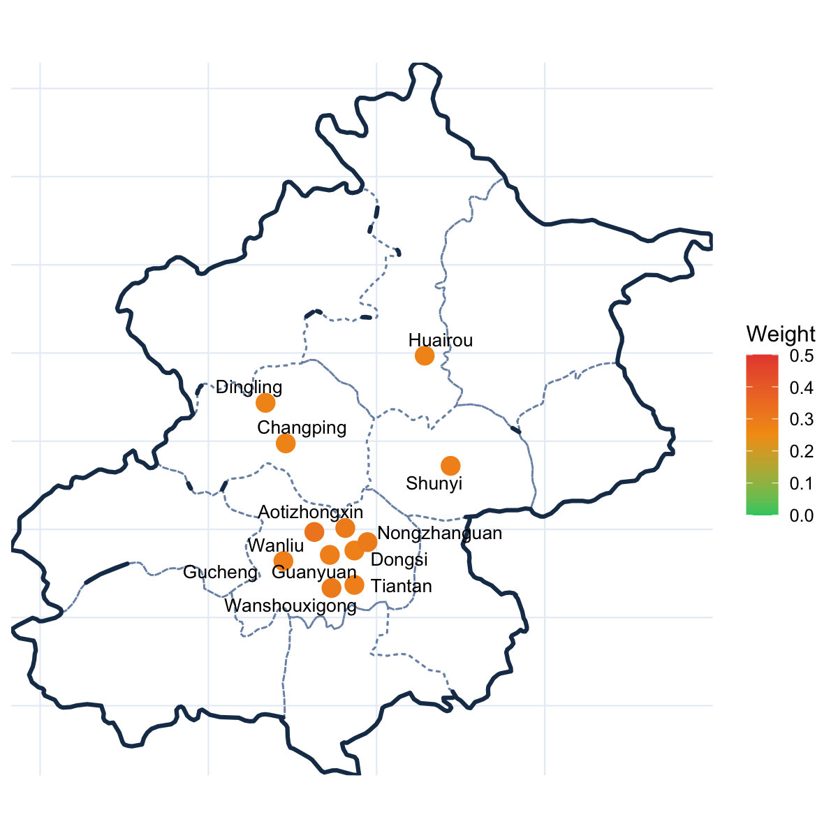
For the monitoring-station mode ( $j=1$ ), Table T3 shows that, for the general pollution factor, Pro.iter and CC-ISO produce broadly similar spatial patterns: all estimated loadings are positive, and both methods assign relatively small estimated loadings to suburban stations such as Dingling and Changping. This is consistent with the interpretation in Section 5 that these stations are located in less polluted areas. By contrast, Pro.init yields a more homogeneous pattern for the general pollution factor, with the estimated loadings of similar magnitude across stations. The HOPE estimates are less regular and include several negative estimated loadings, making the spatial pattern harder to interpret. For the ozone-related factor, all four methods give positive estimated loading vectors.

For the diurnal mode ( $j=3$ ), Figure F7 shows that the four methods give broadly similar estimated loadings for the ozone-related factor. The difference is more pronounced for the general pollution factor. The estimates of Pro.iter exhibit a clear bimodal pattern, with a morning peak and a higher evening peak, which is consistent with the daily cycle of human activity discussed in Section 5. By contrast, the factor loadings estimated by Pro.init, HOPE, and CC-ISO exhibit less plausible bimodal patterns for the general pollution factor. In particular, the estimated factor loadings of these three methods begin to rise as early as around 3:00 a.m., when human activity is still very limited. Moreover, they do not capture the daytime accumulation pattern of general air pollutants; instead, their estimated loadings decline noticeably in the afternoon, which is less consistent with typical daily pollution patterns in urban environments. By comparison, the estimates of Pro.iter are more closely aligned with the known daily patterns of human activity.

As shown in Figure F8, the estimations of the ozone-related factor based on Pro.iter, HOPE, and CC-ISO exhibit a clear seasonal cycle, while this seasonal pattern is much weaker in that of Pro.init. For the general pollution factor, the factor processes estimated by HOPE and CC-ISO exhibit patterns that are nearly opposite to that of Pro.iter. In particular, both methods produce relatively low values in winter, which would imply lower concentrations of general pollutants (PM_2.5, PM₁₀, SO₂, NO₂, and CO) during the cold season. This is difficult to reconcile with the well-known winter pollution pattern in Beijing and is therefore less plausible.

Above comparisons show that, although the four methods can recover the same two pollution patterns, the results based on Pro.iter are more interpretable in terms of their spatial, diurnal, and seasonal structures. This provides further empirical support for the effectiveness of our proposed method.

In addition, we apply the empirical moment test of Trapani 2016 to each marginal series $\{y_{t,\ell_{1},\ell_{2},\ell_{3}}\}_{t=1}^{n}$ ( $\ell_{1}\in[12],\ell_{2}\in[6],\ell_{3}\in[24]$ ). More specifically, for each marginal series, we proceed sequentially as follows: we first test the existence of the 8-th moment; if it is supported by the data, we stop; otherwise, we test the 6-th moment, then finally the 4-th moment. This allows us to determine, for each marginal series, the highest empirically supported finite moment order. We also repeat the same analysis for the 1% winsorized data, obtained by winsorizing each marginal series at the 5‰ lower tail and the 5‰ upper tail. The results reported in Table T4 show that the raw data display some heavy-tailedness. To assess the reliability of our main empirical results, we rerun the real data analysis using the 1% winsorized data. The detailed results are reported in Table T5 and Figures F9–F11. In comparison with the results in Table 3 and Figures 5–7, we can conclude that the resulting estimated factor loadings, factors, and substantive interpretations remain essentially unchanged, indicating that our main empirical conclusions are robust.

Table T4: Proportions of marginal series

\{y_{t,\ell_{1},\ell_{2},\ell_{3}}\}_{t=1}^{n}

(

\ell_{1}\in[12],\ell_{2}\in[6],\ell_{3}\in[24]

) whose highest empirically supported finite moment is at most

k

-th order, based on the test of Trapani 2016 at the 5% significance level.

	$k<4$	$k=4$	$k=6$	$k=8$
raw data	28.76	54.40	12.96	3.88
1% winsorized data	1.68	44.04	26.91	27.37

Table T5: Estimations of the loading vectors

\mathbf{a}_{i,2}\in\mathbb{R}^{6}

for the pollution-variable mode based on Pro.iter using the 1% winsorized data. Standard errors reported in parentheses are calculated based on the asymptotic variance estimation

\hat{w}_{i,j}^{-2}\hat{\tau}_{i,j}^{2}(\mathbf{h})

. ^∗, ^∗∗, and ^∗∗∗ indicate significance at the levels 5%, 1%, and 1‰, respectively, based on two-sided

t

-tests.

Pollutant	$i=1$	$i=2$
PM_2.5	0.014 (0.015)	0.655^∗∗∗ (0.034)
PM₁₀	$-$ 0.019 (0.013)	0.436^∗∗∗ (0.024)
SO₂	0.048^∗∗ (0.016)	0.284^∗∗∗ (0.036)
NO₂	$-$ 0.230^∗∗∗ (0.015)	0.295^∗∗∗ (0.049)
CO	0.187^∗∗∗ (0.012)	0.461^∗∗∗ (0.029)
O₃	0.954^∗∗∗ (0.002)	0.015 (0.078)

B.3 Real data analysis: Fama–French 100 return data

In this section, we illustrate the proposed methods for the tensor CP-factor model (1) using the Fama–French 100 return series. We collect monthly returns from January 1964 to December 2021, yielding 69,600 observations over a total of 696 months. The dataset is obtained from http://mba.tuck.dartmouth.edu/pages/faculty/ken.french/data_library.html. The portfolios are constructed from the intersections of 10 size levels, denoted by $({\rm S}_{1},\ldots,{\rm S}_{10})$ , and 10 levels of the book-to-market equity ratio (BE), denoted by $({\rm BE}_{1},\ldots,{\rm BE}_{10})$ . The dataset contains a small number of missing values in the early years, which we set to zero. Since all 100 series are clearly related to overall market conditions, following Wang et al. 2019, we remove the influence of market effects prior to the empirical analysis by subtracting the corresponding monthly excess market return from each series. The market return data are obtained from the same source.

The 100 market-adjusted return series can be represented as a tensor time series $\mathcal{Y}_{t}=(y_{t,i,j})_{10\times 10}$ for $t\in[696]$ (i.e. $m=2$ , $d_{1}=d_{2}=10$ , $n=696$ ), where $y_{t,i,j}$ is the market-adjusted return at the $i$ -th level of size ${\rm S}_{i}$ and the $j$ -th level of the BE-ratio ${\rm BE}_{j}$ at time $t$ . Figure F12 shows the time series plots of the market-adjusted return series $\{y_{t,i,j}\}_{t=1}^{n}$ for $i,j\in[10]$ . The rows in Figure F12 correspond to the ten levels of size and the columns correspond to the ten levels of the BE-ratio.

a We illustrate the usefulness of our methods by performing one- and two-step-ahead rolling forecasts for the 240 monthly observations in the last twenty years (2002–2021). To estimate the number of factors, following the selection of the tuning parameters in Section 3.4, the log-ER method suggests $\tilde{r}=1$ based on the data $\{\mathcal{Y}_{t}\}_{t=1}^{456}$ , and we use $\tilde{r}=1$ throughout the rolling forecasts. For each $s\in[240]$ , let $\hat{\mathbf{A}}_{j}=\hat{\mathbf{a}}_{1,j}$ for $j\in\{1,2\}$ be the estimated loading vectors based on the data $\{\mathcal{Y}_{t}\}_{t=s}^{455+s}$ . We can then obtain the estimated factor series by $\hat{f}_{t}=(\hat{\mathbf{a}}_{1,2}^{\mathrm{\scriptscriptstyle+}}\otimes\hat{\mathbf{a}}_{1,1}^{\mathrm{\scriptscriptstyle+}})^{\mathrm{\scriptscriptstyle\top}}\textup{vec}(\mathcal{Y}_{t})$ for $t\in\{s,\ldots,455+s\}$ , where $\hat{\mathbf{a}}_{1,j}^{\mathrm{\scriptscriptstyle+}}=\hat{\mathbf{A}}_{j}(\hat{\mathbf{A}}_{j}^{\mathrm{\scriptscriptstyle\top}}\hat{\mathbf{A}}_{j})^{-1}$ for $j\in\{1,2\}$ . To produce the one-step-ahead forecast of $\mathcal{Y}_{456+s}$ , denoted by $\hat{\mathcal{Y}}^{(1)}_{456+s}=(\hat{y}^{(1)}_{456+s,i,j})_{10\times 10}$ , we model the factor process $\{\hat{f}_{t}\}_{t=s}^{455+s}$ . Specifically, for each $s\in[240]$ , we fit an AR model for the factor process $\{\hat{f}_{t}\}_{t=s}^{455+s}$ with the order selected by the Akaike Information Criterion (AIC). For the two-step-ahead forecast, we repeat the above procedure using $\{\mathcal{Y}_{t}\}_{t=s}^{454+s}$ , and the forecast $\hat{\mathcal{Y}}^{(2)}_{456+s}=(\hat{y}^{(2)}_{456+s,i,j})_{10\times 10}$ is then obtained by plugging the one-step-ahead forecasts into the fitted models. Therefore, for each $s\in[240]$ , we can obtain one- and two-step-ahead forecasts of $\mathcal{Y}_{456+s}$ based on the proposed one-pass method (Pro.init) and the iterative method (Pro.iter), respectively. For comparison, we can also fit $\{\mathcal{Y}_{t}\}_{t=s}^{455+s}$ and $\{\mathcal{Y}_{t}\}_{t=s}^{454+s}$ by the following methods and obtain the associated one-step and two-step ahead forecasts:

•

(cPCA, HOPE) The composite PCA and High-Order Projection Estimator in Han et al. 2024b with the recommended tuning parameter $h=1$ therein. We adopt the rank parameter $\tilde{r}=1$ based on the result of our proposed method, and fix $\tilde{r}=1$ in the rolling forecasts. We fit the obtained univariate time series by an AR model with the order determined by the AIC.
•

(RP-PCA, CC-ISO) The Randomized Projection PCA and Contemporary Covariance-based Iterative Simultaneous Orthogonalization in Chen et al. 2026. We estimate the rank parameter $\tilde{r}=1$ based on the data $\{\mathcal{Y}_{t}\}_{t=1}^{456}$ through the unfolded eigenvalue ratio method therein, and fix $\tilde{r}=1$ in the rolling forecasts. The obtained univariate time series is fitted by an AR model with the order determined by the AIC.
•

(RCP) The Refined CP method of Chang et al. 2023 with the pre-determined parameter $K=10$ therein. The associated rank in this method is estimated as $\hat{d}=1$ based on $\{\mathcal{Y}_{t}\}_{t=1}^{456}$ and then fixed in the rolling forecasts. We fit the obtained univariate time series by an AR model with the order determined by the AIC. The method is implemented using the R package HDTSA.
•

(UCP) The Unified CP method of Chang et al. 2026 with the pre-determined parameters $K=20$ and $\tilde{K}=10$ therein. The associated ranks in this method are estimated as $(\hat{d},\hat{d}_{1},\hat{d}_{2})=(2,2,1)$ based on $\{\mathcal{Y}_{t}\}_{t=1}^{456}$ and then fixed in the rolling forecasts. We fit the obtained 2-dimensional time series by a VAR model with the order determined by the AIC. The method is implemented using the R package HDTSA.
•

(FAC) The matrix Tucker-factor model with the FAC method proposed by Wang et al. 2019 with the pre-determined parameter $h_{0}=1$ as suggested therein. The associated ranks in this model are estimated as $(\hat{k}_{1},\hat{k}_{2})=(1,1)$ by the ratio estimators suggested therein based on $\{\mathcal{Y}_{t}\}_{t=1}^{456}$ , and are fixed in the rolling forecasts. We fit the obtained univariate time series by an AR model with the order determined by the AIC.
•

(TOPUP, TIPUP) The Time series Outer-Product Unfolding Procedure and the Time series Inner-Product Unfolding Procedure proposed by Han et al. 2024a for the matrix Tucker-factor model. The associated ranks in this model are estimated as $(\hat{k}_{1},\hat{k}_{2})=(2,2)$ by the information criterion considered in Han et al. 2022 based on $\{\mathcal{Y}_{t}\}_{t=1}^{456}$ , and are fixed in the rolling forecasts. We fit the obtained 4-dimensional time series by a VAR model with the order determined by the AIC. The methods are implemented using the R package tensorTS.
•

(MAR) The matrix-AR(1) model of Chen et al. 2021.
•

(TS-PCA) Apply the principal component analysis for time series proposed by Chang et al. 2018a to the 100-dimensional time series $\{\textup{vec}({\mathcal{Y}}_{t})\}_{t=s}^{455+s}$ and $\{\textup{vec}({\mathcal{Y}}_{t})\}_{t=s}^{454+s}$ , respectively, to obtain the associated one-step and two-step ahead forecasts. The method is implemented using the R package HDTSA. For the obtained univariate time series, we fit it by an AR model with the order determined by the AIC. For the obtained multivariate time series, we fit it by a VAR model with the order determined by the AIC.
•

(UniAR) Fit each of 100 component time series by an AR model with the order determined by the AIC.

For each $s\in[240]$ , the one-step ahead forecasting performance is evaluated by the $\textup{rRMSE}(s)$ and $\textup{rMAE}(s)$ defined as

	$\displaystyle\text{rRMSE}(s)=\bigg\{\frac{1}{100}\sum_{i=1}^{10}\sum_{j=1}^{10}\|\hat{y}^{(1)}_{456+s,i,j}-y_{456+s,i,j}\|^{2}\bigg\}^{1/2}\,,$
	$\displaystyle\text{rMAE}(s)=\frac{1}{100}\sum_{i=1}^{10}\sum_{j=1}^{10}\|\hat{y}^{(1)}_{456+s,i,j}-y_{456+s,i,j}\|\,.$

For the two-step-ahead forecast, the corresponding $\textup{rRMSE}(s)$ and $\textup{rMAE}(s)$ are defined analogously. Table T6 reports the averages of $\{\textup{rRMSE}(s)\}_{s=1}^{240}$ and $\{\textup{rMAE}(s)\}_{s=1}^{240}$ , denoted by rRMSE and rMAE, respectively. The standard deviations of $\{\textup{rRMSE}(s)\}_{s=1}^{240}$ and $\{\textup{rMAE}(s)\}_{s=1}^{240}$ are reported in parentheses. The results show that our proposed methods are promising for forecasting financial returns. In particular, Pro.iter achieves the smallest forecasting errors in the one-step-ahead forecasts, and Pro.init performs very competitively to Pro.iter. For the two-step-ahead forecasts, although the best performance is attained by UCP, both Pro.iter and Pro.init perform very closely to UCP. More broadly, the tensor CP-factor methods without uncorrelated factor assumption (Pro.iter, Pro.init, RCP, and UCP) outperform the methods that rely on this assumption (cPCA and HOPE). It is well known that financial data exhibit strong cross-sectional dependence, and often involve highly correlated latent factors. The results of Table T6 suggest that allowing correlated factors is important for capturing the underlying dependence structure in practice, which provides further evidence on the applicability of our proposed methods.

Table T6: Average forecasting errors and standard deviations (in parentheses) based on different methods. Bold numbers indicate the smallest average forecasting error among all methods.

Method		one-step rRMSE	one-step rMAE	two-step rRMSE	two-step rMAE
Tensor CP-factor methods without uncorrelated factor assumption	Pro.iter	3.4847 (1.6003)	2.6623 (1.1455)	3.4874 (1.5905)	2.6683 (1.1336)
	Pro.init	3.4890 (1.5960)	2.6646 (1.1409)	3.4977 (1.5846)	2.6735 (1.1305)
	RCP	3.5146 (1.5829)	2.6910 (1.1288)	3.5142 (1.5863)	2.6922 (1.1358)
	UCP	3.4905 (1.5698)	2.6676 (1.1133)	3.4869 (1.5685)	2.6674 (1.1170)
	RP-PCA	3.5209 (1.5976)	2.6951 (1.1448)	3.5193 (1.6001)	2.6954 (1.1490)
	CC-ISO	3.5223 (1.5972)	2.6968 (1.1439)	3.5189 (1.5996)	2.6951 (1.1482)
Tensor CP-factor methods with uncorrelated factor assumption	cPCA	3.5293 (1.5883)	2.7047 (1.1333)	3.5239 (1.5926)	2.7013 (1.1408)
	HOPE	3.5255 (1.5876)	2.7008 (1.1327)	3.5208 (1.5943)	2.6982 (1.1422)
Tensor Tucker-factor methods	FAC	3.5470 (1.5789)	2.7143 (1.1250)	3.5413 (1.5817)	2.7130 (1.1323)
	TOPUP	3.5268 (1.5826)	2.7022 (1.1283)	3.5269 (1.5899)	2.7036 (1.1367)
	TIPUP	3.5303 (1.5891)	2.7036 (1.1319)	3.5294 (1.5961)	2.7038 (1.1406)
Other benchmark methods	MAR	3.5154 (1.6093)	2.6923 (1.1597)	3.4959 (1.6057)	2.6765 (1.1539)
	TS-PCA	3.5244 (1.6005)	2.6999 (1.1586)	3.5124 (1.5881)	2.6919 (1.1483)
	UniAR	3.5470 (1.5789)	2.7143 (1.1250)	3.5413 (1.5817)	2.7130 (1.1323)

Appendix C Estimation of factors and common components

The factors and common components may also be of interest in certain scenarios, and they can be estimated by plugging in the estimated factor loading vectors. Specifically, since $w_{i}$ and $f_{t,i}$ in model (1) cannot be identified separately, we directly estimate their product $w_{i}f_{t,i}$ for each $i\in[r]$ and $t\in[n]$ . Given the iterative estimator $\{\hat{\mathbf{a}}_{i,j}\}_{i\in[\tilde{r}],\,j\in[m]}$ , we define $\hat{f}_{t,i}=(\hat{\mathbf{a}}_{i,m}^{\mathrm{\scriptscriptstyle+}}\otimes\cdots\otimes\hat{\mathbf{a}}_{i,1}^{\mathrm{\scriptscriptstyle+}})^{\mathrm{\scriptscriptstyle\top}}\textup{vec}(\mathcal{Y}_{t})$ for $i\in[\tilde{r}]$ and $t\in[n]$ , where $(\hat{\mathbf{a}}_{1,j}^{\mathrm{\scriptscriptstyle+}},\ldots,\hat{\mathbf{a}}_{\tilde{r},j}^{\mathrm{\scriptscriptstyle+}})^{\mathrm{\scriptscriptstyle\top}}=(\hat{\mathbf{A}}_{j}^{\mathrm{\scriptscriptstyle\top}}\hat{\mathbf{A}}_{j})^{-1}\hat{\mathbf{A}}_{j}^{\mathrm{\scriptscriptstyle\top}}$ with $\hat{\mathbf{A}}_{j}=(\hat{\mathbf{a}}_{1,j},\ldots,\hat{\mathbf{a}}_{\tilde{r},j})$ . Therefore, the factors $(w_{1}f_{t,1},\ldots,w_{r}f_{t,r})$ are then estimated by $(\hat{f}_{t,1},\ldots,\hat{f}_{t,\tilde{r}})$ . In model (1), we write $\mathcal{C}_{t}=\sum_{i=1}^{r}w_{i}{f}_{t,i}\,\mathbf{a}_{i,1}\circ\mathbf{a}_{i,2}\circ\cdots\circ\mathbf{a}_{i,m}$ and estimate it by $\hat{\mathcal{C}}_{t}=\sum_{i=1}^{\tilde{r}}\hat{f}_{t,i}\,\hat{\mathbf{a}}_{i,1}\circ\hat{\mathbf{a}}_{i,2}\circ\cdots\circ\hat{\mathbf{a}}_{i,m}$ . Write $\Phi_{n}=\max_{j\in[m]}\Phi_{n,j}+\gamma_{\max}w_{r}^{-2}$ . Theorem T2 establishes the consistency of these estimators.

Theorem T2.

Let the conditions of Theorem 3 hold. For each fixed $i\in[r]$ and $t\in[n]$ , it holds that

	$\displaystyle\frac{1}{w_{i}}\bigg\|\bigg(\prod_{j=1}^{m}\kappa_{i,j}\bigg)\hat{f}_{t,z_{i}}-w_{i}f_{t,i}\bigg\|$	$\displaystyle=O_{\rm p}\bigg(\frac{1}{w_{i}}+\Phi_{n}\bigg)\,,$
	$\displaystyle\frac{1}{D_{n}}\|\textup{vec}(\hat{\mathcal{C}}_{t})-\textup{vec}(\mathcal{C}_{t})\|^{2}_{2}$	$\displaystyle=O_{\rm p}\bigg(\frac{1}{D_{n}}+\frac{w_{1}^{2}}{D_{n}}\Phi_{n}^{2}\bigg)\,,$

where $z_{i}$ and $\kappa_{i,j}$ are specified in Theorem 3.

Theorem T2 indicates that the convergence rate of the factor estimator comprises two components. The first component, $O_{\rm p}(w_{i}^{-1})$ , originates from the noise $\mathcal{E}_{t}$ and also appears in Han et al. 2024b. The second component arises from the plug-in errors of $\{\hat{\mathbf{a}}_{i,j}\}_{i\in[\tilde{r}],j\in[m]}$ . When $w_{i}\max_{j\in[m]}(s_{j}\log d_{j})^{1/2}\ll w_{r}\sqrt{n}$ and $\gamma_{\max}w_{i}\ll w_{r}^{2}$ , the rate $O_{\rm p}(w_{i}^{-1})$ dominates. The convergence rate of the estimated common component tensor depends on both the estimation errors of the loadings and the factors.

Next, we conduct simulation studies to compare the finite-sample performance of the methods discussed in the paper (Pro.iter, HOPE, CC-ISO, Pro.init, cPCA, RP-PCA, and RCP) in estimating the common components. The data-generating process follows the setup in Section 4. The estimation error between the estimated common components $\{\check{\mathcal{C}}_{t}\}_{t\in[n]}$ and the true common components $\{\mathcal{C}_{t}\}_{t\in[n]}$ is measured by

\psi^{2}_{\textup{cp}}(\{\check{\mathcal{C}}_{t}\}_{t\in[n]},\{\mathcal{C}_{t}\}_{t\in[n]})=\bigg\{\frac{1}{nD_{n}}\sum_{t=1}^{n}|\textup{vec}(\check{\mathcal{C}}_{t})-\textup{vec}(\mathcal{C}_{t})|_{2}^{2}\bigg\}^{1/2}\,.

(S.8)

As shown in Table T7, when $\rho=0$ , Pro.iter performs comparably with CC-ISO and HOPE, and significantly outperforms the other methods. When $\rho=0.75$ , Pro.iter outperforms both CC-ISO and HOPE. Moreover, Pro.init outperforms all other one-pass estimators across all scenarios. These results confirm that the proposed methods also have good performance in estimating the common components in finite samples.

Table T7: The averages and standard deviations (in parentheses) of the estimation errors (S.8) of common components for different methods based on 2000 repetitions. Bold numbers indicate the smallest average estimation error among all competing methods.

$\rho$	$\phi$	$s$	$n$	Iterative estimates			One-pass estimates
$\rho$	$\phi$	$s$	$n$	Pro.iter	HOPE	CC-ISO	Pro.init	cPCA	RP-PCA	RCP
0	0.25	0	400	0.12 (0.05)	0.12 (0.09)	0.12 (0.11)	0.39 (1.14)	0.87 (0.64)	0.96 (0.67)	0.62 (0.49)
		0	800	0.11 (0.07)	0.12 (0.08)	0.11 (0.09)	0.26 (0.23)	0.76 (0.56)	0.86 (0.60)	0.54 (0.46)
		0.3	400	0.11 (0.06)	0.12 (0.11)	0.11 (0.08)	0.35 (0.19)	0.79 (0.63)	0.86 (0.67)	0.58 (0.47)
		0.3	800	0.11 (0.05)	0.11 (0.07)	0.11 (0.09)	0.26 (0.75)	0.68 (0.58)	0.75 (0.62)	0.52 (0.45)
		0.6	400	0.10 (0.03)	0.11 (0.11)	0.11 (0.10)	0.33 (0.18)	0.73 (0.67)	0.79 (0.69)	0.57 (0.46)
		0.6	800	0.10 (0.03)	0.10 (0.05)	0.11 (0.09)	0.23 (0.48)	0.58 (0.58)	0.65 (0.63)	0.51 (0.45)
	0.75	0	400	0.25 (0.15)	0.26 (0.19)	0.23 (0.12)	0.80 (1.11)	1.35 (0.35)	1.42 (0.38)	1.05 (0.47)
		0	800	0.23 (0.09)	0.25 (0.17)	0.24 (0.15)	0.59 (2.19)	1.40 (0.32)	1.45 (0.37)	1.07 (0.48)
		0.3	400	0.14 (0.06)	0.15 (0.10)	0.15 (0.10)	0.49 (0.72)	1.18 (0.53)	1.28 (0.51)	0.76 (0.53)
		0.3	800	0.14 (0.05)	0.15 (0.11)	0.15 (0.12)	0.32 (0.44)	1.21 (0.49)	1.34 (0.48)	0.79 (0.55)
		0.6	400	0.12 (0.04)	0.12 (0.10)	0.12 (0.08)	0.36 (0.31)	0.88 (0.64)	0.94 (0.66)	0.62 (0.49)
		0.6	800	0.11 (0.05)	0.12 (0.08)	0.12 (0.07)	0.24 (0.25)	0.77 (0.55)	0.88 (0.61)	0.56 (0.47)
0.75	0.25	0	400	0.15 (0.03)	0.32 (0.31)	0.33 (0.31)	0.39 (0.42)	1.81 (0.72)	1.84 (0.73)	0.42 (0.42)
		0	800	0.13 (0.01)	0.30 (0.30)	0.31 (0.30)	0.24 (0.28)	1.79 (0.66)	1.81 (0.67)	0.40 (0.41)
		0.3	400	0.14 (0.01)	0.32 (0.31)	0.34 (0.32)	0.35 (0.26)	1.87 (0.79)	1.90 (0.79)	0.43 (0.44)
		0.3	800	0.12 (0.01)	0.34 (0.32)	0.34 (0.32)	0.22 (0.21)	1.89 (0.75)	1.91 (0.75)	0.39 (0.40)
		0.6	400	0.13 (0.03)	0.34 (0.33)	0.35 (0.33)	0.34 (0.24)	1.96 (0.88)	1.99 (0.87)	0.43 (0.95)
		0.6	800	0.11 (0.02)	0.36 (0.33)	0.36 (0.33)	0.21 (0.15)	1.97 (0.89)	1.99 (0.86)	0.40 (0.41)
	0.75	0	400	0.30 (0.13)	0.29 (0.19)	0.68 (0.34)	0.71 (0.76)	1.40 (0.38)	1.09 (0.37)	0.51 (0.41)
		0	800	0.24 (0.06)	0.26 (0.17)	0.48 (0.33)	0.48 (0.66)	1.41 (0.34)	1.21 (0.41)	0.42 (0.40)
		0.3	400	0.18 (0.07)	0.26 (0.25)	0.32 (0.32)	0.48 (0.58)	1.58 (0.55)	1.55 (0.59)	0.41 (0.39)
		0.3	800	0.15 (0.02)	0.25 (0.24)	0.27 (0.25)	0.32 (0.97)	1.56 (0.54)	1.56 (0.55)	0.39 (0.41)
		0.6	400	0.14 (0.04)	0.30 (0.30)	0.31 (0.31)	0.43 (1.44)	1.76 (0.69)	1.77 (0.72)	0.42 (0.43)
		0.6	800	0.12 (0.02)	0.32 (0.31)	0.32 (0.31)	0.23 (0.26)	1.77 (0.71)	1.78 (0.70)	0.38 (0.40)

Appendix D Further discussion on the estimated number of factors

D.1 Consistency of the estimators of the number of factors

Theorem T3 shows that the ER and log-ER estimators specified in (20) and (21) are consistent estimators for the number of factors $r$ .

Theorem T3.

Set the threshold level $\delta_{1}=C_{*}(n^{-1}\log D_{n})^{1/2}$ in (8) for some constant $C_{*}>0$ . Under Assumptions 1–6, if $\log D_{n}\ll n^{c}$ for some constant $c\in(0,1)$ depending only on $c_{1}$ and $c_{2}$ specified in Assumptions 2 and 3, as $n\to\infty$ , the following two assertions hold.

(i) Let $\underaccent{\bar}{\sigma}_{\xi}^{2}\Pi_{n}\ll c_{n}\ll\bar{\sigma}_{\xi}^{-2}\underaccent{\bar}{\sigma}_{\xi}^{4}$ for the $c_{n}$ in (20). Then

\mathbb{P}\Big\{\max_{j\in[m]}\tilde{r}^{(\textup{er})}_{j}(\delta_{1})=r\Big\}\rightarrow 1\,.

(ii) Let $\log(1+\underaccent{\bar}{\sigma}_{\xi}^{2}\Pi_{n})\ll c_{n}\ll\{\log(1+\bar{\sigma}_{\xi}^{2})\}^{-1}\{\log(1+\underaccent{\bar}{\sigma}_{\xi}^{2})\}^{2}$ for the $c_{n}$ in (21). Then

\mathbb{P}\Big\{\max_{j\in[m]}\tilde{r}^{(\textup{log})}_{j}(\delta_{1})=r\Big\}\rightarrow 1\,.

The conditions imposed on $c_{n}$ ensure a proper separation between the signal part and the noise part. In particular, the requirement $\underaccent{\bar}{\sigma}_{\xi}^{2}\Pi_{n}\ll c_{n}\ll\bar{\sigma}_{\xi}^{-2}\underaccent{\bar}{\sigma}_{\xi}^{4}$ (and its counterpart for the log-ER criterion) guarantees that the estimation error is asymptotically negligible relative to the eigen-gap.

D.2 Effects of misspecifying the number of factors

As shown in Theorem T3, our proposed estimators for the number of factors are consistent. However, the estimated number of factors may still deviate from the true value in finite samples. It is therefore critical to examine the robustness of our proposed estimation procedures against such misspecification.

Let $\tilde{r}$ be the estimate of $r$ involved in our estimation procedures. Recall $r=3$ in our simulation studies considered in Section 4. To mimic the misspecification issue of $r$ , we vary $\tilde{r}$ from $1$ to $10$ , and continue to evaluate the estimation error defined in (22) in Section 4. The corresponding results based on Pro.iter and Pro.init are reported in Figure F13. It can be observed that (i) when $\tilde{r}<r$ , both methods perform poorly because some true factors are omitted; (ii) when $\tilde{r}=r$ , both methods achieve their best performance; and (iii) when $\tilde{r}>r$ , the error of the one-pass method (Pro.init) increases, whereas the iterative method (Pro.iter) is almost unaffected. Note that, even when $\tilde{r}>r$ , the measure (22) still remains small as long as the estimated loading vectors contain accurate estimates of the true loading vectors. The results in Figure F13 suggest that, although $\tilde{r}>r$ leads to an over-fitted factor structure, our iterative estimator (Pro.iter) can still recover all the true loading vectors well, which indicates that our proposed iterative estimator is reasonably robust to the issue with an overestimated number of factors.

As shown in Table 1 in Section 4, the proposed log-ER estimator may underestimate $r$ in finite samples, although the frequency is small. In practice, to reduce the chance that the estimated number of factors is smaller than the true value $r$ , we can apply a two-stage procedure. In the first stage, we apply the log-ER estimator and the Pro.iter method to $\{\mathcal{Y}_{t}\}_{t=1}^{n}$ to get the first-stage estimated number of factors $\tilde{r}^{(1)}$ and the associated estimation of the loading vectors, and then obtain the estimated idiosyncratic error tensor sequence $\{\hat{\mathcal{E}}_{t}\}_{t=1}^{n}$ . In the second stage, we apply the log-ER estimator to $\{\hat{\mathcal{E}}_{t}\}_{t=1}^{n}$ to obtain the second-stage estimated number of factors $\tilde{r}^{(2)}$ . Based on these two stages, we can select $\tilde{r}=\tilde{r}^{(1)}+\tilde{r}^{(2)}$ as the estimate of $r$ . Table T8 reports the performance of one-stage procedure (log-ER estimator) and two-stage procedure introduced above, respectively. The results show that the proposed two-stage procedure rarely underestimates $r$ in finite samples. Combining these findings with the results in Figure F13, we conclude that the proposed iterative method, with $\tilde{r}$ obtained by the two-stage procedure, is reasonably robust to misspecification of $r$ .

Table T8: Relative frequency estimates of

\mathbb{P}(\tilde{r}<r)

and

\mathbb{P}(\tilde{r}\geq r)

based on 2000 repetitions, where

\tilde{r}

is obtained from the one-stage and two-stage procedures. All numbers reported below are multiplied by 100.

$\rho$	$\phi$	$s$	$n$	One-stage procedure		Two-stage procedure
$\rho$	$\phi$	$s$	$n$	$\mathbb{P}(\tilde{r}<r)$	$\mathbb{P}(\tilde{r}\geq r)$	$\mathbb{P}(\tilde{r}<r)$	$\mathbb{P}(\tilde{r}\geq r)$
0	0.25	0	400	0.25	99.75	0.00	100.00
		0	800	0.65	99.35	0.00	100.00
		0.3	400	0.40	99.60	0.00	100.00
		0.3	800	0.40	99.60	0.00	100.00
		0.6	400	0.10	99.90	0.00	100.00
		0.6	800	0.55	99.45	0.00	100.00
	0.75	0	400	4.55	95.45	0.00	100.00
		0	800	1.60	98.40	0.00	100.00
		0.3	400	0.60	99.40	0.00	100.00
		0.3	800	0.35	99.65	0.00	100.00
		0.6	400	0.10	99.90	0.00	100.00
		0.6	800	0.20	99.80	0.00	100.00
0.75	0.25	0	400	0.10	99.90	0.00	100.00
		0	800	0.00	100.00	0.00	100.00
		0.3	400	0.00	100.00	0.00	100.00
		0.3	800	0.00	100.00	0.00	100.00
		0.6	400	0.15	99.85	0.00	100.00
		0.6	800	0.00	100.00	0.00	100.00
	0.75	0	400	13.80	86.20	0.10	99.90
		0	800	0.55	99.45	0.00	100.00
		0.3	400	0.65	99.35	0.00	100.00
		0.3	800	0.00	100.00	0.00	100.00
		0.6	400	0.15	99.85	0.00	100.00
		0.6	800	0.00	100.00	0.00	100.00

Appendix E Proofs of Theorems 1–3, and Theorems T1–T3

To simplify the notation, we use $\mathbf{o}_{\rm p}(\cdot)$ and $\mathbf{O}_{\rm p}(\cdot)$ to denote matrices (or vectors) whose spectral norms are $o_{\rm p}(\cdot)$ and $O_{\rm p}(\cdot)$ , respectively. For a matrix $\mathbf{H}$ , denote by $\mathcal{M}(\mathbf{H})$ the linear space spanned by the columns of $\mathbf{H}$ .

E.1 Proof of Theorem 1

The proof is divided into two steps. Step 1 shows the consistency of $\tilde{\mathbf{Q}}_{j}$ specified in Section 3.1. Step 2 completes the proof of the consistency of $\tilde{\mathbf{a}}_{i,j}$ .

E.1.1 Step 1: Consistency of $\tilde{\mathbf{Q}}_{j}$

We start with the truncated matrix $\tilde{\bm{\Sigma}}_{k,j}$ defined in (8). By definition, $\tilde{\bm{\Sigma}}_{k,j}=T_{\delta_{1}}\{\tilde{\bm{\Sigma}}_{\mathbf{Y}_{j},\xi}(k)\}$ , where $\tilde{\bm{\Sigma}}_{\mathbf{Y}_{j},\xi}(k)=\tilde{\bm{\Sigma}}_{\mathbf{C}_{j},\xi}(k)+\tilde{\bm{\Sigma}}_{\mathbf{E}_{j},\xi}(k)$ with

	$\displaystyle\tilde{\bm{\Sigma}}_{\mathbf{C}_{j},\xi}(k)$	$\displaystyle=\frac{1}{n-k}\sum_{t=k+1}^{n}(\mathbf{C}_{t,j}-\bar{\mathbf{C}}_{j})(\xi_{t-k}-\bar{\xi})\,,~~\bar{\mathbf{C}}_{j}=\frac{1}{n}\sum_{t=1}^{n}\mathbf{C}_{t,j}\,,$		(S.9)
	$\displaystyle\tilde{\bm{\Sigma}}_{\mathbf{E}_{j},\xi}(k)$	$\displaystyle=\frac{1}{n-k}\sum_{t=k+1}^{n}(\mathbf{E}_{t,j}-\bar{\mathbf{E}}_{j})(\xi_{t-k}-\bar{\xi})\,,~~\bar{\mathbf{E}}_{j}=\frac{1}{n}\sum_{t=1}^{n}\mathbf{E}_{t,j}\,,$		(S.10)

and $\mathbf{C}_{t,j}$ , $\mathbf{E}_{t,j}$ are specified in (2). Let $\tilde{\mathbf{G}}_{k,\xi}=\textup{diag}(\tilde{g}_{k,1,\xi},\ldots,\tilde{g}_{k,r,\xi})$ be the sample version of $\mathbf{G}_{k,\xi}$ defined above (5), where

\tilde{g}_{k,i,\xi}=\frac{1}{n-k}\sum_{t=k+1}^{n}w_{i}(f_{t,i}-\bar{f}_{i})(\xi_{t-k}-\bar{\xi})\,.

(S.11)

Then, it follows that $\tilde{\bm{\Sigma}}_{\mathbf{C}_{j},\xi}(k)=\mathbf{A}_{j}\tilde{\mathbf{G}}_{k,\xi}\mathbf{B}_{j}^{\mathrm{\scriptscriptstyle\top}}$ . To prove the consistency of $\tilde{\mathbf{Q}}_{j}$ , we need Lemmas L1–L3. The proofs of Lemmas L1–L3 are given in Sections F.1–F.3, respectively.

Lemma L1.

If $\textup{rank}(\mathbf{A}_{j})=r$ for $j\in[m]$ , it holds that $\textup{rank}(\mathbf{B}_{j})=r$ for $j\in[m]$ . Moreover, under Assumption 4, it holds that $\sigma_{1}(\mathbf{B}_{j}),\ldots,\sigma_{r}(\mathbf{B}_{j})$ are uniformly bounded away from $0$ and $\infty$ .

Lemma L2.

Under Assumptions 2 and 3, for any $i\in[r]$ , it holds that

\max_{k\in[K]}|\tilde{g}_{k,i,\xi}-g_{k,i,\xi}|=O_{\rm p}(w_{i}n^{-1/2})\,,

(S.12)

provided that $\log D_{n}\ll n^{c}$ for some constant $c\in(0,1)$ depending only on $c_{1}$ and $c_{2}$ specified in Assumptions 2 and 3, where $g_{k,i,\xi}$ and $\tilde{g}_{k,i,\xi}$ are defined in (5) and (S.11), respectively.

Lemma L3.

Let Assumptions 1–5 hold and $\delta_{1}=C_{*}(n^{-1}\log D_{n})^{1/2}$ for some sufficiently large constant $C_{*}>0$ . It holds that

\|T_{\delta_{1}}\{\tilde{\bm{\Sigma}}_{\mathbf{Y}_{j},\xi}(k)\}-\tilde{\bm{\Sigma}}_{\mathbf{C}_{j},\xi}(k)\|_{2}=\underaccent{\bar}{\sigma}_{\xi}^{2}\bar{\sigma}_{\xi}^{-1}O_{\rm p}(\Pi_{n})

for any $k\in[K]$ , provided that $\log D_{n}\ll n^{c}$ for some constant $c\in(0,1)$ depending only on $c_{1}$ and $c_{2}$ specified in Assumptions 2 and 3, where $\tilde{\bm{\Sigma}}_{\mathbf{C}_{j},\xi}(k)$ is defined in (S.9).

Since $\tilde{\bm{\Sigma}}_{\mathbf{C}_{j},\xi}(k)=\mathbf{A}_{j}\tilde{\mathbf{G}}_{k,\xi}\mathbf{B}_{j}^{\mathrm{\scriptscriptstyle\top}}$ , following Lemmas L1 and L2, and Assumptions 4 and 5, by Triangle inequality and Cauchy–Schwarz inequality, we have

\|\tilde{\bm{\Sigma}}_{\mathbf{C}_{j},\xi}(k)\|_{2}\lesssim\max_{i\in[r]}|\tilde{g}_{k,i,\xi}|\lesssim\bar{\sigma}_{\xi}\{1+o_{\rm p}(1)\}\,.

(S.13)

Following Lemma L3 and (S.13), by the definition of $\tilde{\mathbf{M}}_{j}$ , Triangle inequality, and Cauchy–Schwarz inequality, and using the fact that $(\underaccent{\bar}{\sigma}_{\xi}^{2}\bar{\sigma}_{\xi}^{-1}\Pi_{n})^{2}\lesssim\underaccent{\bar}{\sigma}_{\xi}^{2}\Pi_{n}$ under the condition $\Pi_{n}\ll 1$ , it holds that

\bigg\|\tilde{\mathbf{M}}_{j}-\sum_{k=1}^{K}\tilde{\bm{\Sigma}}_{\mathbf{C}_{j},\xi}(k)^{\mathrm{\scriptscriptstyle\top}}\tilde{\bm{\Sigma}}_{\mathbf{C}_{j},\xi}(k)\bigg\|_{2}=\underaccent{\bar}{\sigma}_{\xi}^{2}\,O_{\rm p}(\Pi_{n})\,.

(S.14)

On the other hand, by Lemma L2 and Triangle inequality, we also have

\bigg\|\sum_{k=1}^{K}\tilde{\bm{\Sigma}}_{\mathbf{C}_{j},\xi}(k)^{\mathrm{\scriptscriptstyle\top}}\tilde{\bm{\Sigma}}_{\mathbf{C}_{j},\xi}(k)-\sum_{k=1}^{K}\bm{\Sigma}_{\mathbf{Y}_{j},\xi}(k)^{\mathrm{\scriptscriptstyle\top}}\bm{\Sigma}_{\mathbf{Y}_{j},\xi}(k)\bigg\|_{2}=O_{\rm p}(w_{1}\bar{\sigma}_{\xi}n^{-1/2})\,.

(S.15)

Under Assumption 5, we have $w_{1}\bar{\sigma}_{\xi}n^{-1/2}\ll\underaccent{\bar}{\sigma}_{\xi}^{2}$ . Meanwhile, all the nonzero eigenvalues of $\sum_{k=1}^{K}\bm{\Sigma}_{\mathbf{Y}_{j},\xi}(k)^{\mathrm{\scriptscriptstyle\top}}\bm{\Sigma}_{\mathbf{Y}_{j},\xi}(k)$ are lower bounded by $\underaccent{\bar}{\sigma}_{\xi}^{2}$ . Therefore, by Weyl’s theorem, we conclude that the minimum nonzero eigenvalue of $\sum_{k=1}^{K}\tilde{\bm{\Sigma}}_{\mathbf{C}_{j},\xi}(k)^{\mathrm{\scriptscriptstyle\top}}\tilde{\bm{\Sigma}}_{\mathbf{C}_{j},\xi}(k)$ is larger than $\underaccent{\bar}{\sigma}_{\xi}^{2}\{1-o_{\rm p}(1)\}$ . Furthermore, note that

\sum_{k=1}^{K}\tilde{\bm{\Sigma}}_{\mathbf{C}_{j},\xi}(k)^{\mathrm{\scriptscriptstyle\top}}\tilde{\bm{\Sigma}}_{\mathbf{C}_{j},\xi}(k)=\mathbf{Q}_{j}\mathbf{V}_{j}\bigg(\sum_{k=1}^{K}\tilde{\mathbf{G}}_{k,\xi}\mathbf{A}_{j}^{\mathrm{\scriptscriptstyle\top}}\mathbf{A}_{j}\tilde{\mathbf{G}}_{k,\xi}\bigg)\mathbf{V}_{j}^{\mathrm{\scriptscriptstyle\top}}\mathbf{Q}_{j}^{\mathrm{\scriptscriptstyle\top}}\,,

whose $r$ leading eigenvectors are in $\mathcal{M}(\mathbf{Q}_{j})$ . Recall $\tilde{r}=r$ . Therefore, by (S.14) and standard results in perturbation theory, see e.g. Lemma 1 of Chang et al. 2018a, we conclude that

\|\tilde{\mathbf{Q}}_{j}-\mathbf{Q}_{j}\tilde{\mathcal{H}}_{j}\|_{2}=O_{\rm p}(\Pi_{n})

(S.16)

for some orthogonal matrix $\tilde{\mathcal{H}}_{j}$ , provided that $\log D_{n}\ll n^{c}$ for some constant $c\in(0,1)$ depending only on $c_{1}$ and $c_{2}$ specified in Assumptions 2 and 3.

E.1.2 Step 2: Consistency of $\tilde{\mathbf{a}}_{i,j}$

By definition, $\tilde{\mathbf{a}}_{i,j}$ is an eigenvector of $\tilde{\mathbf{K}}_{1,2,j}$ , while $\mathbf{a}_{i,j}$ is an associated eigenvector of $\mathbf{K}_{1,2,j}$ . Following the perturbation theory for eigen-analysis, such as Lemma 4 in Chang et al. 2023, to prove the consistency of $\tilde{\mathbf{a}}_{i,j}$ , we should start with the consistency of $\tilde{\mathbf{K}}_{1,2,j}$ under spectral norm.

We will not bound the error $\|\tilde{\mathbf{K}}_{1,2,j}-\mathbf{K}_{1,2,j}\|_{2}$ directly. Instead, similarly to the definition of $\mathbf{K}_{1,2,j}$ in (6), we define $\hat{\mathbf{K}}_{1,2,j}$ by replacing $\bm{\Sigma}_{\mathbf{Y}_{j},\xi}(k)$ with $\tilde{\bm{\Sigma}}_{\mathbf{C}_{j},\xi}(k)=\mathbf{A}_{j}\tilde{\mathbf{G}}_{k,\xi}\mathbf{B}_{j}^{\mathrm{\scriptscriptstyle\top}}$ for $k\in\{1,2\}$ , where the diagonal entries of $\tilde{\mathbf{G}}_{k,\xi}$ are defined in (S.11). Similarly to $\mathbf{K}_{1,2,j}=\mathbf{A}_{j}\mathbf{G}_{1,\xi}\mathbf{G}_{2,\xi}^{-1}(\mathbf{A}_{j}^{\mathrm{\scriptscriptstyle\top}}\mathbf{A}_{j})^{-1}\mathbf{A}_{j}^{\mathrm{\scriptscriptstyle\top}}$ , we have

\hat{\mathbf{K}}_{1,2,j}=\mathbf{A}_{j}\tilde{\mathbf{G}}_{1,\xi}\tilde{\mathbf{G}}_{2,\xi}^{-1}(\mathbf{A}_{j}^{\mathrm{\scriptscriptstyle\top}}\mathbf{A}_{j})^{-1}\mathbf{A}_{j}^{\mathrm{\scriptscriptstyle\top}}\,.

(S.17)

Hence, $\mathbf{a}_{i,j}$ is also an eigenvector of $\hat{\mathbf{K}}_{1,2,j}$ with the associated eigenvalue $\hat{\lambda}_{i}=\tilde{g}_{2,i,\xi}^{-1}\tilde{g}_{1,i,\xi}$ . To complete the proof of Theorem 1, we need the following lemma with its proof given in Section F.4.

Lemma L4.

Under Assumptions 1–6, there exist a $d_{j}\times(d_{j}-1)$ matrix $\mathbf{O}_{j,\scalebox{1}{\text{-}}i}$ and a universal constant $C_{10}>0$ such that $(\mathbf{a}_{i,j},\mathbf{O}_{j,\scalebox{1}{\text{-}}i})$ is an orthogonal matrix and

\begin{split}\sigma_{\min}\{\mathbf{O}_{j,\scalebox{1}{\text{-}}i}^{\mathrm{\scriptscriptstyle\top}}(\mathbf{K}_{1,2,j}-\bar{\lambda}_{i}\mathbf{I}_{d_{j}})\mathbf{O}_{j,\scalebox{1}{\text{-}}i}\}&\geq C_{10}\,,\\ \sigma_{\min}\{\mathbf{O}_{j,\scalebox{1}{\text{-}}i}^{\mathrm{\scriptscriptstyle\top}}(\hat{\mathbf{K}}_{1,2,j}-\hat{\lambda}_{i}\mathbf{I}_{d_{j}})\mathbf{O}_{j,\scalebox{1}{\text{-}}i}\}&\geq C_{10}\{1-o_{\rm p}(1)\}\,,\end{split}

where $\hat{\mathbf{K}}_{1,2,j}$ is defined in (S.17) with the associated eigenvalues $\hat{\lambda}_{i}=\tilde{g}_{2,i,\xi}^{-1}\tilde{g}_{1,i,\xi}$ for $i\in[r]$ . In addition, $\hat{\lambda}_{i}=\bar{\lambda}_{i}+o_{\rm p}(1)$ for $i\in[r]$ .

By Lemma L4, following the perturbation theory from Lemma 4 of Chang et al. 2023, it remains to bound the error $\|\tilde{\mathbf{K}}_{1,2,j}-\hat{\mathbf{K}}_{1,2,j}\|_{2}$ . According to the definition of $\tilde{\mathbf{K}}_{1,2,j}$ , we first investigate the minimum eigenvalue of $\tilde{\mathbf{Q}}_{j}^{\mathrm{\scriptscriptstyle\top}}\tilde{\bm{\Sigma}}_{2,j}^{\mathrm{\scriptscriptstyle\top}}\tilde{\bm{\Sigma}}_{2,j}\tilde{\mathbf{Q}}_{j}$ . By Lemma L3 and (S.13), we have

\|\tilde{\mathbf{Q}}_{j}^{\mathrm{\scriptscriptstyle\top}}\tilde{\bm{\Sigma}}_{2,j}^{\mathrm{\scriptscriptstyle\top}}\tilde{\bm{\Sigma}}_{2,j}\tilde{\mathbf{Q}}_{j}-\tilde{\mathbf{Q}}_{j}^{\mathrm{\scriptscriptstyle\top}}\tilde{\bm{\Sigma}}_{\mathbf{C}_{j},\xi}(2)^{\mathrm{\scriptscriptstyle\top}}\tilde{\bm{\Sigma}}_{\mathbf{C}_{j},\xi}(2)\tilde{\mathbf{Q}}_{j}\|_{2}=\underaccent{\bar}{\sigma}_{\xi}^{2}O_{\rm p}(\Pi_{n})\,.

(S.18)

Therefore, we should consider the minimum eigenvalue of $\tilde{\mathbf{Q}}_{j}^{\mathrm{\scriptscriptstyle\top}}\tilde{\bm{\Sigma}}_{\mathbf{C}_{j},\xi}(2)^{\mathrm{\scriptscriptstyle\top}}\tilde{\bm{\Sigma}}_{\mathbf{C}_{j},\xi}(2)\tilde{\mathbf{Q}}_{j}$ . By (S.16), $\tilde{\mathbf{Q}}_{j}$ is a consistent estimator of $\mathbf{Q}_{j}\tilde{\mathcal{H}}_{j}$ . Then, because $\sigma_{\min}(\tilde{\mathcal{H}}_{j}^{\mathrm{\scriptscriptstyle\top}}\mathbf{Q}_{j}^{\mathrm{\scriptscriptstyle\top}}\mathbf{B}_{j})\geq C$ for some universal constant $C>0$ , we can conclude that $\sigma_{\min}(\tilde{\mathbf{Q}}_{j}^{\mathrm{\scriptscriptstyle\top}}\mathbf{B}_{j})\geq C\{1-o_{\rm p}(1)\}$ . It follows that

\begin{split}\sigma_{\min}\{\tilde{\mathbf{Q}}_{j}^{\mathrm{\scriptscriptstyle\top}}\tilde{\bm{\Sigma}}_{\mathbf{C}_{j},\xi}(2)^{\mathrm{\scriptscriptstyle\top}}\tilde{\bm{\Sigma}}_{\mathbf{C}_{j},\xi}(2)\tilde{\mathbf{Q}}_{j}\}&=\sigma_{\min}(\tilde{\mathbf{Q}}_{j}^{\mathrm{\scriptscriptstyle\top}}\mathbf{B}_{j}\tilde{\mathbf{G}}_{2,\xi}\mathbf{A}_{j}^{\mathrm{\scriptscriptstyle\top}}\mathbf{A}_{j}\tilde{\mathbf{G}}_{2,\xi}\mathbf{B}_{j}^{\mathrm{\scriptscriptstyle\top}}\tilde{\mathbf{Q}}_{j})\\ &\gtrsim\underaccent{\bar}{\sigma}_{\xi}^{2}\{1-o_{\rm p}(1)\}\,.\end{split}

(S.19)

Then, by (S.18), (S.19) and Weyl’s Theorem, we can further conclude that

\sigma_{\min}(\tilde{\mathbf{Q}}_{j}^{\mathrm{\scriptscriptstyle\top}}\tilde{\bm{\Sigma}}_{2,j}^{\mathrm{\scriptscriptstyle\top}}\tilde{\bm{\Sigma}}_{2,j}\tilde{\mathbf{Q}}_{j})\gtrsim\underaccent{\bar}{\sigma}_{\xi}^{2}\{1-o_{\rm p}(1)\}\,.

(S.20)

Next, for any $p\times p$ invertible matrices $\mathbf{W}_{1}$ and $\mathbf{W}_{2}$ , it holds that

\mathbf{W}_{1}^{-1}=\mathbf{W}_{2}^{-1}-\mathbf{W}_{1}^{-1}(\mathbf{W}_{1}-\mathbf{W}_{2})\mathbf{W}_{2}^{-1}=\mathbf{W}_{2}^{-1}\{\mathbf{I}_{p}+(\mathbf{W}_{1}-\mathbf{W}_{2})\mathbf{W}_{2}^{-1}\}^{-1}\,.

(S.21)

Combining (S.18) with (S.21), we have

\begin{split}&\tilde{\bm{\Sigma}}_{\mathbf{C}_{j},\xi}(1)\tilde{\mathbf{Q}}_{j}(\tilde{\mathbf{Q}}_{j}^{\mathrm{\scriptscriptstyle\top}}\tilde{\bm{\Sigma}}_{2,j}^{\mathrm{\scriptscriptstyle\top}}\tilde{\bm{\Sigma}}_{2,j}\tilde{\mathbf{Q}}_{j})^{-1}\\ &~~~~~~~~=\tilde{\bm{\Sigma}}_{\mathbf{C}_{j},\xi}(1)\tilde{\mathbf{Q}}_{j}\{\tilde{\mathbf{Q}}_{j}^{\mathrm{\scriptscriptstyle\top}}\tilde{\bm{\Sigma}}_{\mathbf{C}_{j},\xi}(2)^{\mathrm{\scriptscriptstyle\top}}\tilde{\bm{\Sigma}}_{\mathbf{C}_{j},\xi}(2)\tilde{\mathbf{Q}}_{j}\}^{-1}\{\mathbf{I}_{r}+\mathbf{o}_{\rm p}(1)\}^{-1}\,.\end{split}

Then, by direct calculation, it holds that

\begin{split}\|\tilde{\bm{\Sigma}}_{\mathbf{C}_{j},\xi}(1)\tilde{\mathbf{Q}}_{j}(\tilde{\mathbf{Q}}_{j}^{\mathrm{\scriptscriptstyle\top}}\tilde{\bm{\Sigma}}_{2,j}^{\mathrm{\scriptscriptstyle\top}}\tilde{\bm{\Sigma}}_{2,j}\tilde{\mathbf{Q}}_{j})^{-1}\|_{2}=O_{\rm p}(\underaccent{\bar}{\sigma}_{\xi}^{-1})\,.\end{split}

Further by Lemma L3, (S.20), and Triangle inequality, we also have

\|\tilde{\bm{\Sigma}}_{k,j}\tilde{\mathbf{Q}}_{j}(\tilde{\mathbf{Q}}_{j}^{\mathrm{\scriptscriptstyle\top}}\tilde{\bm{\Sigma}}_{2,j}^{\mathrm{\scriptscriptstyle\top}}\tilde{\bm{\Sigma}}_{2,j}\tilde{\mathbf{Q}}_{j})^{-1}\|_{2}=O_{\rm p}(\underaccent{\bar}{\sigma}_{\xi}^{-1})\,,\quad k\in\{1,2\}\,.

(S.22)

Now, by Lemma L3 and (S.22), it follows that

\begin{split}\tilde{\mathbf{K}}_{1,2,j}=\tilde{\bm{\Sigma}}_{1,j}\tilde{\mathbf{Q}}_{j}(\tilde{\mathbf{Q}}_{j}^{\mathrm{\scriptscriptstyle\top}}\tilde{\bm{\Sigma}}_{2,j}^{\mathrm{\scriptscriptstyle\top}}\tilde{\bm{\Sigma}}_{2,j}\tilde{\mathbf{Q}}_{j})^{-1}\tilde{\mathbf{Q}}_{j}^{\mathrm{\scriptscriptstyle\top}}\tilde{\bm{\Sigma}}_{\mathbf{C}_{j},\xi}(2)^{\mathrm{\scriptscriptstyle\top}}+\frac{\underaccent{\bar}{\sigma}_{\xi}}{\bar{\sigma}_{\xi}}\mathbf{O}_{\rm p}(\Pi_{n})\,.\end{split}

(S.23)

Using (S.21) once again, we obtain

		$\displaystyle(\tilde{\mathbf{Q}}_{j}^{\mathrm{\scriptscriptstyle\top}}\tilde{\bm{\Sigma}}_{2,j}^{\mathrm{\scriptscriptstyle\top}}\tilde{\bm{\Sigma}}_{2,j}\tilde{\mathbf{Q}}_{j})^{-1}\tilde{\mathbf{Q}}_{j}^{\mathrm{\scriptscriptstyle\top}}\tilde{\bm{\Sigma}}_{\mathbf{C}_{j},\xi}(2)^{\mathrm{\scriptscriptstyle\top}}$
		$\displaystyle~~~~=\{\tilde{\mathbf{Q}}_{j}^{\mathrm{\scriptscriptstyle\top}}\tilde{\bm{\Sigma}}_{\mathbf{C}_{j},\xi}(2)^{\mathrm{\scriptscriptstyle\top}}\tilde{\bm{\Sigma}}_{\mathbf{C}_{j},\xi}(2)\tilde{\mathbf{Q}}_{j}\}^{-1}\tilde{\mathbf{Q}}_{j}^{\mathrm{\scriptscriptstyle\top}}\tilde{\bm{\Sigma}}_{\mathbf{C}_{j},\xi}(2)^{\mathrm{\scriptscriptstyle\top}}$
		$\displaystyle~~~~\quad-(\tilde{\mathbf{Q}}_{j}^{\mathrm{\scriptscriptstyle\top}}\tilde{\bm{\Sigma}}_{2,j}^{\mathrm{\scriptscriptstyle\top}}\tilde{\bm{\Sigma}}_{2,j}\tilde{\mathbf{Q}}_{j})^{-1}\tilde{\mathbf{Q}}_{j}^{\mathrm{\scriptscriptstyle\top}}\{\tilde{\bm{\Sigma}}_{2,j}^{\mathrm{\scriptscriptstyle\top}}\tilde{\bm{\Sigma}}_{2,j}-\tilde{\bm{\Sigma}}_{\mathbf{C}_{j},\xi}(2)^{\mathrm{\scriptscriptstyle\top}}\tilde{\bm{\Sigma}}_{\mathbf{C}_{j},\xi}(2)\}\tilde{\mathbf{Q}}_{j}$
		$\displaystyle~~~~\quad\quad\cdot\{\tilde{\mathbf{Q}}_{j}^{\mathrm{\scriptscriptstyle\top}}\tilde{\bm{\Sigma}}_{\mathbf{C}_{j},\xi}(2)^{\mathrm{\scriptscriptstyle\top}}\tilde{\bm{\Sigma}}_{\mathbf{C}_{j},\xi}(2)\tilde{\mathbf{Q}}_{j}\}^{-1}\tilde{\mathbf{Q}}_{j}^{\mathrm{\scriptscriptstyle\top}}\tilde{\bm{\Sigma}}_{\mathbf{C}_{j},\xi}(2)^{\mathrm{\scriptscriptstyle\top}}$
		$\displaystyle~~~~=(\mathbf{B}_{j}^{\mathrm{\scriptscriptstyle\top}}\tilde{\mathbf{Q}}_{j})^{-1}\tilde{\mathbf{G}}_{2,\xi}^{-1}(\mathbf{A}_{j}^{\mathrm{\scriptscriptstyle\top}}\mathbf{A}_{j})^{-1}\mathbf{A}_{j}^{\mathrm{\scriptscriptstyle\top}}$
		$\displaystyle~~~~\quad-(\tilde{\mathbf{Q}}_{j}^{\mathrm{\scriptscriptstyle\top}}\tilde{\bm{\Sigma}}_{2,j}^{\mathrm{\scriptscriptstyle\top}}\tilde{\bm{\Sigma}}_{2,j}\tilde{\mathbf{Q}}_{j})^{-1}\tilde{\mathbf{Q}}_{j}^{\mathrm{\scriptscriptstyle\top}}\{\tilde{\bm{\Sigma}}_{2,j}-\tilde{\bm{\Sigma}}_{\mathbf{C}_{j},\xi}(2)\}^{\mathrm{\scriptscriptstyle\top}}\mathbf{A}_{j}(\mathbf{A}_{j}^{\mathrm{\scriptscriptstyle\top}}\mathbf{A}_{j})^{-1}\mathbf{A}_{j}^{\mathrm{\scriptscriptstyle\top}}$
		$\displaystyle~~~~\quad-(\tilde{\mathbf{Q}}_{j}^{\mathrm{\scriptscriptstyle\top}}\tilde{\bm{\Sigma}}_{2,j}^{\mathrm{\scriptscriptstyle\top}}\tilde{\bm{\Sigma}}_{2,j}\tilde{\mathbf{Q}}_{j})^{-1}\tilde{\mathbf{Q}}_{j}^{\mathrm{\scriptscriptstyle\top}}\tilde{\bm{\Sigma}}_{2,j}^{\mathrm{\scriptscriptstyle\top}}\{\tilde{\bm{\Sigma}}_{2,j}-\tilde{\bm{\Sigma}}_{\mathbf{C}_{j},\xi}(2)\}\tilde{\mathbf{Q}}_{j}(\mathbf{B}_{j}^{\mathrm{\scriptscriptstyle\top}}\tilde{\mathbf{Q}}_{j})^{-1}\tilde{\mathbf{G}}_{2,\xi}^{-1}(\mathbf{A}_{j}^{\mathrm{\scriptscriptstyle\top}}\mathbf{A}_{j})^{-1}\mathbf{A}_{j}^{\mathrm{\scriptscriptstyle\top}}\,.$

Left-multiplying both sides by $\tilde{\bm{\Sigma}}_{1,j}\tilde{\mathbf{Q}}_{j}$ , and combining with Lemma L3, (S.22) and (S.23), we can conclude that

\tilde{\mathbf{K}}_{1,2,j}-\frac{\underaccent{\bar}{\sigma}_{\xi}}{\bar{\sigma}_{\xi}}\mathbf{O}_{\rm p}(\Pi_{n})=\hat{\mathbf{K}}_{1,2,j}+\frac{\underaccent{\bar}{\sigma}_{\xi}}{\bar{\sigma}_{\xi}}\mathbf{O}_{\rm p}(\Pi_{n})+\tilde{\mathbf{K}}_{1,2,j}\cdot\frac{\underaccent{\bar}{\sigma}_{\xi}}{\bar{\sigma}_{\xi}}\mathbf{O}_{\rm p}(\Pi_{n})\,,

where we use the fact $\hat{\mathbf{K}}_{1,2,j}=\tilde{\bm{\Sigma}}_{\mathbf{C}_{j},\xi}(1)\tilde{\mathbf{Q}}_{j}\{\tilde{\mathbf{Q}}_{j}^{\mathrm{\scriptscriptstyle\top}}\tilde{\bm{\Sigma}}_{\mathbf{C}_{j},\xi}(2)^{\mathrm{\scriptscriptstyle\top}}\tilde{\bm{\Sigma}}_{\mathbf{C}_{j},\xi}(2)\tilde{\mathbf{Q}}_{j}\}^{-1}\tilde{\mathbf{Q}}_{j}^{\mathrm{\scriptscriptstyle\top}}\tilde{\bm{\Sigma}}_{\mathbf{C}_{j},\xi}(2)^{\mathrm{\scriptscriptstyle\top}}$ . Consequently, we have

\|\tilde{\mathbf{K}}_{1,2,j}-\hat{\mathbf{K}}_{1,2,j}\|_{2}=\frac{\underaccent{\bar}{\sigma}_{\xi}}{\bar{\sigma}_{\xi}}O_{\rm p}(\Pi_{n})\,.

(S.24)

Then, Theorem 1 follows from Lemma L4, (S.24), and standard perturbation theory; see Lemma 4 of Chang et al. 2023. $\hfill\Box$

E.2 Proof of Theorem 2

The proof is divided into three steps. Step 1 constructs an event to control some random quantities. Step 2 shows how the iterations improve the convergence rate in each round. Step 3 completes the proof of Theorem 2 by letting the number of iterations grow gradually. For notational simplicity, the proofs of Steps 1–3 in Sections E.2.1–E.2.3 ignore the reflection and permutation indeterminacy and focus on the case $r\geq 2$ . Section E.2.4 further discusses the impact of the reflection and permutation indeterminacy, and shows that the proof for the case $r=1$ is trivial and follows directly as a specialization of the argument for $r\geq 2$ .

E.2.1 Step 1: Construct an event to bound some random quantities

Recall that $\tilde{r}=r$ . Define $\theta_{j}^{(\textit{v})}=\max_{i\in[r]}|\tilde{\mathbf{a}}_{i,j}^{(\textit{v})}-\mathbf{a}_{i,j}|_{2}$ , which measures the estimation error of $\tilde{\mathbf{A}}_{j}^{(\textit{v})}=(\tilde{\mathbf{a}}_{1,j}^{(\textit{v})},\ldots,\tilde{\mathbf{a}}_{r,j}^{(\textit{v})})$ obtained after the v-th round of the iteration in Algorithm 1. Write

\bar{\theta}_{j}^{(\textit{v})}=\max(\theta_{1}^{(\textit{v})},\ldots,\theta_{j-1}^{(\textit{v})},\theta_{j}^{(\textit{v}-1)},\ldots,\theta_{m}^{(\textit{v}-1)})\,,\quad\textit{v}\geq 1,\,j\in[m]\,.

(S.25)

It is important to construct the relationship between $\theta_{j}^{(\textit{v})}$ and $\bar{\theta}_{j}^{(\textit{v})}$ . To do this, for some constant $\tilde{C}>0$ that specified later, we first define a series of events

$\displaystyle\Xi_{1,n}(\tilde{C})$	$\displaystyle=\bigg\{\bigg\|\frac{1}{n-k-k_{1}-k_{2}}\sum_{t=k+k_{1}+1}^{n-k_{2}}(f_{t,i}-\bar{f}_{i})(f_{t-k,\ell}-\bar{f}_{\ell})-\Upsilon_{k,i,\ell}\bigg\|<\tilde{C}^{-1}$
	$\displaystyle\qquad\qquad\qquad\qquad\qquad\qquad\textup{for any}~i,\ell\in[r]~\textup{and}~k,k_{1},k_{2}\in\{0,1\}\bigg\}\,,$
$\displaystyle\Xi_{2,n}(\tilde{C})$	$\displaystyle=\bigg\{\bigg\|\frac{1}{n-k-k_{1}-k_{2}}\sum_{t=k+k_{1}+1}^{n-k_{2}}[(f_{t,i}-\bar{f}_{i})\xi_{t-k,\ell}^{\textup{s}}-\mathbb{E}\{(f_{t,i}-\bar{f}_{i})\xi_{t-k,\ell}^{\textup{s}}\}]\bigg\|<\tilde{C}^{-1}$
	$\displaystyle\qquad\qquad\qquad\qquad\qquad\qquad\textup{for any}~i,\ell\in[r]~\textup{and}~k,k_{1},k_{2}\in\{0,1\}\bigg\}\,,$
$\displaystyle\Xi_{3,n}(\tilde{C})$	$\displaystyle=\bigg\{\frac{1}{n-1}\\|(\mathbf{F}_{\xi,\scalebox{1}{\text{-}}i}^{\textup{s}})^{\mathrm{\scriptscriptstyle\top}}\mathbf{F}_{\xi,\scalebox{1}{\text{-}}i}^{\textup{s}}-\mathbb{E}\{(\mathbf{F}_{\xi,\scalebox{1}{\text{-}}i}^{\textup{s}})^{\mathrm{\scriptscriptstyle\top}}\mathbf{F}_{\xi,\scalebox{1}{\text{-}}i}^{\textup{s}}\}\\|_{2}<\tilde{C}^{-1}~\textup{for any}~i\in[r]\bigg\}\,,$
$\displaystyle\Xi_{4,n}(\tilde{C})$	$\displaystyle=\bigg\{\frac{1}{n-1}\|(\mathbf{F}_{\xi,\scalebox{1}{\text{-}}i}^{\textup{s}})^{\mathrm{\scriptscriptstyle\top}}\bm{\xi}_{i}^{\textup{s}}-\mathbb{E}\{(\mathbf{F}_{\xi,\scalebox{1}{\text{-}}i}^{\textup{s}})^{\mathrm{\scriptscriptstyle\top}}\bm{\xi}_{i}^{\textup{s}}\}\|_{2}<\tilde{C}^{-1}~\textup{for any}~i\in[r]\bigg\}\,,$
$\displaystyle\Xi_{5,n}(\tilde{C})$	$\displaystyle=\bigg\{\bigg\|\frac{1}{n-k_{1}-k_{2}}\sum_{t=k_{1}+1}^{n-k_{2}}[(\xi_{t,i}-\bar{\xi}_{i})^{2}-\mathbb{E}\{(\xi_{t,i}-\bar{\xi}_{i})^{2}\}]\bigg\|<w_{i}^{2}\tilde{C}^{-1}$	(S.26)
	$\displaystyle\qquad\qquad\qquad\qquad\qquad\qquad\textup{for any}~i\in[r]~\textup{and}~k_{1},k_{2}\in\{0,1\}\bigg\}\,.$

For $L_{n}$ specified in (24), let $\Xi_{6,n}(\tilde{C})$ be the event such that

\begin{split}&\max_{\begin{subarray}{c}|\bm{\beta}_{j}|_{2}=1,\,\bm{\beta}_{j}\in\mathbb{R}^{d_{j}},\\ \forall j\in[m]\end{subarray}}\bigg|\frac{1}{n-k-k_{1}-k_{2}}\sum_{t=k+k_{1}+1}^{n-k_{2}}(f_{t-k,i}-\bar{f}_{i})(\mathcal{E}_{t}\times_{j=1}^{m}\bm{\beta}_{j}^{\mathrm{\scriptscriptstyle\top}})\bigg|\,\leq\tilde{C}L_{n}\,\end{split}

(S.27)

for any $i\in[r]$ and $k,k_{1},k_{2}\in\{0,1\}$ , where $\times_{j=1}^{m}\bm{\beta}_{j}^{\mathrm{\scriptscriptstyle\top}}$ is shorthand for $\times_{1}\bm{\beta}_{1}^{\mathrm{\scriptscriptstyle\top}}\times_{2}\cdots\times_{m}\bm{\beta}_{m}^{\mathrm{\scriptscriptstyle\top}}$ with $\times_{j}$ defined as the $j$ -mode product of a tensor and a matrix. In detail, for a tensor $\mathcal{A}\in\mathbb{R}^{d_{1}\times\cdots\times d_{m}}$ and a matrix $\bm{\beta}\in\mathbb{R}^{d_{0}\times d_{j}}$ , $\mathcal{A}\times_{j}\bm{\beta}$ is still an $m$ -mode tensor of size $d_{1}\times\cdots\times d_{j-1}\times d_{0}\times d_{j+1}\times\cdots\times d_{m}$ with the entries being

[\mathcal{A}\times_{j}\bm{\beta}]_{i_{1},\ldots,i_{m}}=\sum_{h=1}^{d_{j}}[\mathcal{A}]_{i_{1},\ldots,i_{j-1},h,i_{j+1},\ldots,i_{m}}[\bm{\beta}]_{i_{j},h}\,.

Let $\Xi_{7,n}(\tilde{C})$ be the event such that

\begin{split}&\max_{\begin{subarray}{c}|\tilde{\bm{\beta}}_{j}|_{2}=1=|\bm{\beta}_{j}|_{2},\\ \tilde{\bm{\beta}}_{j},\,\bm{\beta}_{j}\in\mathbb{R}^{d_{j}},\forall j\in[m]\end{subarray}}\bigg|\frac{1}{n-1}\sum_{t=2}^{n}(\mathcal{E}_{t-1}\times_{j=1}^{m}\tilde{\bm{\beta}}_{j}^{\mathrm{\scriptscriptstyle\top}})(\mathcal{E}_{t}\times_{j=1}^{m}\bm{\beta}_{j}^{\mathrm{\scriptscriptstyle\top}})\bigg|\leq\tilde{C}L_{n}\,.\end{split}

(S.28)

Let $\Xi_{8,n}(\tilde{C})$ be the event such that

\max_{|\bm{\beta}_{j}|_{2}=1,\,\bm{\beta}_{j}\in\mathbb{R}^{d_{j}},\forall j\in[m]}\bigg|\frac{1}{n-k_{1}-k_{2}}\sum_{t=k_{1}+1}^{n-k_{2}}\mathcal{E}_{t}\times_{j=1}^{m}\bm{\beta}_{j}^{\mathrm{\scriptscriptstyle\top}}\bigg|\leq\tilde{C}L_{n}

(S.29)

for $k_{1},k_{2}\in\{0,1\}$ . Let $\Xi_{9,n}(\tilde{C})$ be the event such that

		$\displaystyle\max_{\begin{subarray}{c}\|\tilde{\bm{\beta}}_{j}\|_{2}=1=\|\bm{\beta}_{j}\|_{2},\\ \tilde{\bm{\beta}}_{j},\,\bm{\beta}_{j}\in\mathbb{R}^{d_{j}},\forall j\in[m]\end{subarray}}\bigg\|\frac{1}{n-k_{1}-k_{2}}\sum_{t=k_{1}+1}^{n-k_{2}}(\otimes^{j=1}_{m}\tilde{\bm{\beta}}_{j})^{\mathrm{\scriptscriptstyle\top}}[\text{vec}(\mathcal{E}_{t})\text{vec}(\mathcal{E}_{t})^{\mathrm{\scriptscriptstyle\top}}$
		$\displaystyle\qquad\qquad\qquad\qquad\qquad\qquad\qquad-\mathbb{E}\{\text{vec}(\mathcal{E}_{t})\text{vec}(\mathcal{E}_{t})^{\mathrm{\scriptscriptstyle\top}}\}](\otimes^{j=1}_{m}\bm{\beta}_{j})\bigg\|\leq\tilde{C}L_{n}$		(S.30)

for $k_{1},k_{2}\in\{0,1\}$ , where $\otimes^{j=1}_{m}\bm{\beta}_{j}$ is shorthand for $\bm{\beta}_{m}\otimes\cdots\otimes\bm{\beta}_{1}$ .

Let $\Xi_{n}(\tilde{C})=\cap_{h=1}^{9}\Xi_{h,n}(\tilde{C})$ . Lemma L5 shows that $\mathbb{P}\{\Xi_{n}(\tilde{C})\}\rightarrow 1$ as $n\rightarrow\infty$ for some sufficiently large constant $\tilde{C}>0$ . The proof of Lemma L5 is given in Section F.5.

Lemma L5.

Under the assumptions of Theorem 2, there exists a sufficiently large constant $C_{0}>0$ such that $\mathbb{P}\{\Xi_{n}(\tilde{C})\}\rightarrow 1$ as $n\rightarrow\infty$ for any constant $\tilde{C}>C_{0}$ .

E.2.2 Step 2: Error reduction across iterations

Now, for the v-th iteration round and the $j$ -th mode, let $\bar{\check{f}}_{i}^{(\textit{v},j)}=n^{-1}\sum_{t=1}^{n}\check{f}_{t,i}^{(\textit{v},j)}$ , where $\check{f}_{t,i}^{(\textit{v},j)}$ is defined in Algorithm 1. Further let

(\tilde{\sigma}^{(\textit{v},j)}_{\check{f},i})^{2}=\frac{1}{n-1}\sum_{t=1}^{n}(\check{f}_{t,i}^{(\textit{v},j)}-\bar{\check{f}}_{i}^{(\textit{v},j)})^{2}\,.

Define $\tilde{\mathbf{F}}_{\scalebox{1}{\text{-}}i}^{(\textit{v},j)}$ and $\tilde{\mathbf{f}}_{i}^{(\textit{v},j)}$ by similar steps above (13) but replacing $\check{f}_{t,i}$ with $\check{f}_{t,i}^{(\textit{v},j)}$ . Furthermore, let $\tilde{\bm{\varphi}}_{i}^{(\textit{v},j)}=(\tilde{\varphi}_{i,1}^{(\textit{v},j)},\ldots,\tilde{\varphi}_{i,r}^{(\textit{v},j)})^{\mathrm{\scriptscriptstyle\top}}$ be the $r$ -dimensional vector with the $i$ -th entry equal to 1, and the remaining $r-1$ entries form the vector $-\{(\tilde{\mathbf{F}}_{\scalebox{1}{\text{-}}i}^{(\textit{v},j)})^{\mathrm{\scriptscriptstyle\top}}\tilde{\mathbf{F}}_{\scalebox{1}{\text{-}}i}^{(\textit{v},j)}\}^{-1}(\tilde{\mathbf{F}}_{\scalebox{1}{\text{-}}i}^{(\textit{v},j)})^{\mathrm{\scriptscriptstyle\top}}\tilde{\mathbf{f}}_{i}^{(\textit{v},j)}$ . Let $\bm{\Lambda}_{\xi}=(\Lambda_{\xi,i,j})_{r\times r}$ be the $r\times r$ diagonal matrix with the $i$ -th diagonal entry being $n^{-1}\sum_{t=1}^{n}\mathbb{E}\{(\xi_{t,i}-\bar{\xi}_{i})^{2}\}$ . Define

	$\displaystyle\bm{\zeta}_{1}^{(i,j,\textit{v})}$	$\displaystyle=\bigg\{\frac{w_{i}}{n-1}\sum_{t=2}^{n}(f_{t,i}-\bar{f}_{i})\tilde{\xi}_{t-1,i}^{(\textit{v},j)}\bigg\}\{\mathbf{b}_{i,j}^{\mathrm{\scriptscriptstyle\top}}(\tilde{\mathbf{b}}_{i,j}^{(\textit{v})})^{\mathrm{\scriptscriptstyle+}}\}\mathbf{a}_{i,j}\,,$
	$\displaystyle\bm{\zeta}_{2}^{(i,j,\textit{v})}$	$\displaystyle=\sum_{\ell\neq i}\bigg\{\frac{w_{\ell}}{n-1}\sum_{t=2}^{n}(f_{t,\ell}-\bar{f}_{\ell})\tilde{\xi}_{t-1,i}^{(\textit{v},j)}\bigg\}\{\mathbf{b}_{\ell,j}^{\mathrm{\scriptscriptstyle\top}}(\tilde{\mathbf{b}}_{i,j}^{(\textit{v})})^{\mathrm{\scriptscriptstyle+}}\}\mathbf{a}_{\ell,j}\,,$
	$\displaystyle\bm{\zeta}_{3}^{(i,j,\textit{v})}$	$\displaystyle=\frac{\Lambda_{\xi,i,i}^{1/2}}{\tilde{\sigma}^{(\textit{v},j)}_{\check{f},i}}\tilde{\bm{\Sigma}}_{\mathbf{e}_{i,j},\xi_{i}}(1)+\sum_{\ell\neq i}\frac{\tilde{\varphi}_{i,\ell}^{(\textit{v},j)}\Lambda_{\xi,\ell,\ell}^{1/2}}{\tilde{\sigma}_{\check{f},\ell}^{(\textit{v},j)}}\tilde{\bm{\Sigma}}_{\mathbf{e}_{i,j},\xi_{\ell}}(0)\,,$
	$\displaystyle\bm{\zeta}_{4}^{(i,j,\textit{v})}$	$\displaystyle=\bigg\{\frac{1}{n-1}\sum_{t=2}^{n}\tilde{\xi}_{t-1,i}^{(\textit{v},j)}(\mathbf{E}_{t,j}-\bar{\mathbf{E}}_{j})(\tilde{\mathbf{b}}_{i,j}^{(\textit{v})})^{\mathrm{\scriptscriptstyle+}}\bigg\}-\bm{\zeta}_{3}^{(i,j,\textit{v})}\,.$

Then, for each $i\in[r]$ and $j\in[m]$ , we have

\begin{split}\tilde{\bm{\Sigma}}^{(\textit{v},j)}_{\tilde{\mathbf{y}}_{i,j},\tilde{\xi}_{i}}(1)=\bm{\zeta}_{1}^{(i,j,\textit{v})}+\bm{\zeta}_{2}^{(i,j,\textit{v})}+\bm{\zeta}_{3}^{(i,j,\textit{v})}+\bm{\zeta}_{4}^{(i,j,\textit{v})}\,,\end{split}

(S.31)

where $\tilde{\bm{\Sigma}}^{(\textit{v},j)}_{\tilde{\mathbf{y}}_{i,j},\tilde{\xi}_{i}}(1)$ is defined in Algorithm 1. Recall the estimator

\tilde{\mathbf{a}}_{i,j}^{(\textit{v})}=T_{\delta_{2,j}}\{\tilde{\bm{\Sigma}}^{(\textit{v},j)}_{\tilde{\mathbf{y}}_{i,j},\tilde{\xi}_{i}}(1)\}/|T_{\delta_{2,j}}\{\tilde{\bm{\Sigma}}^{(\textit{v},j)}_{\tilde{\mathbf{y}}_{i,j},\tilde{\xi}_{i}}(1)\}|_{2}\,.

To calculate the estimation error of $\tilde{\mathbf{a}}_{i,j}^{(\textit{v})}$ , we need the following results shown in Lemmas L6–L9, where the involved constant $\tilde{C}_{0}>0$ is independent of $\tilde{C}$ and $(i,j,\textit{v})$ that may vary in different lemmas. The proofs of Lemmas L6–L9 are given in Sections F.6–F.9, respectively.

Lemma L6.

Under the assumptions of Theorem 2 and $r\geq 2$ , for any $i\neq\ell$ , as $n\rightarrow\infty$ , we have $\bar{\varphi}_{i,\ell}=O(\gamma_{\max}+n^{-1}w_{r}^{-2})$ , where $\bar{\varphi}_{i,\ell}$ is defined below (23).

Lemma L7.

Under the assumptions of Theorem 2 and the event $\Xi_{n}(\tilde{C})=\cap_{h=1}^{9}\Xi_{h,n}(\tilde{C})$ for a sufficiently large constant $\tilde{C}>0$ , given $j\in[m]$ and $\textit{v}\geq 1$ , if $w_{r}^{-1}w_{1}\bar{\theta}_{j}^{(\textit{v})}\leq\tilde{C}^{-2}$ and $r\geq 2$ , it holds for all $i,\ell\in[r]$ that

\bigg|\frac{\Lambda_{\xi,i,i}^{1/2}}{\tilde{\sigma}^{(\textit{v},j)}_{\check{f},i}}-1\bigg|\leq\tilde{C}_{0}\tilde{C}^{-1}~~\textup{and}~~|\tilde{\varphi}_{i,\ell}^{(\textit{v},j)}-\bar{\varphi}_{i,\ell}|\leq\tilde{C}_{0}\tilde{C}^{-1}

as $n\to\infty$ , where $\tilde{C}_{0}>0$ is a constant independent of $\tilde{C}$ and $(i,j,\textit{v})$ , and $\bar{\varphi}_{i,\ell}$ is defined below (23).

Lemma L8.

Under the same assumptions as in Lemma L7, it holds for all $i\in[r]$ that

\bigg|\frac{1}{w_{i}\sigma_{f_{i},\xi_{i}}}\bm{\zeta}_{1}^{(i,j,\textit{v})}-\mathbf{a}_{i,j}\bigg|_{2}\leq\tilde{C}_{0}\tilde{C}^{-1/2}

as $n\to\infty$ , where $\tilde{C}_{0}>0$ is a constant independent of $\tilde{C}$ and $(i,j,\textit{v})$ , and $\sigma_{f_{i},\xi_{i}}$ is defined in (24).

Lemma L9.

Under the same assumptions as in Lemma L7, it holds for all $i\in[r]$ that

\begin{split}|\bm{\zeta}_{2}^{(i,j,\textit{v})}|_{2}+|\bm{\zeta}_{4}^{(i,j,\textit{v})}|_{2}&\leq\tilde{C}_{0}\tilde{C}\bigg(\frac{\gamma_{\max}+\Delta_{0,n}}{w_{r}}+\frac{1}{nw_{r}^{3}}\bigg)\\ &\quad+\tilde{C}_{0}\tilde{C}\bigg(\frac{w_{1}}{w_{i}}\bar{\theta}_{j}^{(\textit{v})}+\frac{w_{1}}{w_{i}w_{r}}L_{n}\bigg)w_{i}\bar{\theta}_{j}^{(\textit{v})}\end{split}

(S.32)

as $n\to\infty$ , where $\tilde{C}_{0}>0$ is a constant independent of $\tilde{C}$ and $(i,j,\textit{v})$ , $L_{n}$ is defined in (24), and

\begin{split}\Delta_{0,n}&=\max_{i\in[r]}\frac{1}{n-1}|(\mathbf{F}_{\xi,\scalebox{1}{\text{-}}i}^{\textup{s}})^{\mathrm{\scriptscriptstyle\top}}\bm{\xi}_{i}^{\textup{s}}-\mathbb{E}\{(\mathbf{F}_{\xi,\scalebox{1}{\text{-}}i}^{\textup{s}})^{\mathrm{\scriptscriptstyle\top}}\bm{\xi}_{i}^{\textup{s}}\}|_{2}\\ &\quad+\max_{i,\ell\in[r]}\bigg|\frac{1}{n-1}\sum_{t=2}^{n}(f_{t,i}-\bar{f}_{i})(f_{t-1,\ell}-\bar{f}_{\ell})-\frac{1}{n-1}\sum_{t=2}^{n}\mathbb{E}\{(f_{t,i}-\bar{f}_{i})(f_{t-1,\ell}-\bar{f}_{\ell})\}\bigg|\,.\end{split}

The above lemmas serve as preliminaries for deriving the upper bound of $\theta_{j}^{(\textit{v})}$ . To proceed, we need to further define several random quantities. Recall the vectors $\tilde{\bm{\Sigma}}_{\mathbf{e}_{\ell,j},\xi_{i}}(1)$ and $\tilde{\bm{\Sigma}}_{\mathbf{e}_{\ell,j},\xi_{i}}(0)$ defined in (26). Let

\begin{split}\Delta_{1,n,j}&=\max_{i,\ell\in[r]}\{|\tilde{\bm{\Sigma}}_{\mathbf{e}_{\ell,j},\xi_{i}}(1)|_{\max}+|\tilde{\bm{\Sigma}}_{\mathbf{e}_{\ell,j},\xi_{i}}(0)|_{\max}\}\,,\\ \Delta_{2,n,j}(x)&=\max_{i,\ell\in[r]}\sum_{p=1}^{d_{j}}I\{|[\tilde{\bm{\Sigma}}_{\mathbf{e}_{\ell,j},\xi_{i}}(1)]_{p}|+|[\tilde{\bm{\Sigma}}_{\mathbf{e}_{\ell,j},\xi_{i}}(0)]_{p}|>x(n^{-1}\log d_{j})^{1/2}\}\end{split}

(S.33)

for $x>0$ , where $[\cdot]_{p}$ stands for the $p$ -th entry of a vector. Lemma L10 below provides an error bound for $|T_{\delta_{2,j}}\{\tilde{\bm{\Sigma}}^{(\textit{v},j)}_{\tilde{\mathbf{y}}_{i,j},\tilde{\xi}_{i}}(1)\}-\bm{\zeta}_{1}^{(i,j,\textit{v})}|_{2}$ , whose proof is given in Section F.10 and relies on the previous results in Lemmas L6–L9.

Lemma L10.

Under the same assumptions in Lemma L7, by setting the threshold level in Algorithm 1 as $\delta_{2,j}=\tilde{C}_{*}(n^{-1}\log d_{j})^{1/2}$ for some sufficiently large constant $\tilde{C}_{*}>0$ , it holds for all $i\in[r]$ that

\begin{split}|T_{\delta_{2,j}}\{\tilde{\bm{\Sigma}}^{(\textit{v},j)}_{\tilde{\mathbf{y}}_{i,j},\tilde{\xi}_{i}}(1)\}-\bm{\zeta}_{1}^{(i,j,\textit{v})}|_{2}&\leq\tilde{C}_{0}\tilde{C}\bigg\{w_{r}\Delta_{n,j}+\frac{1}{w_{r}}\bigg(\gamma_{\max}+\Delta_{0,n}+\frac{1}{nw_{r}^{2}}\bigg)\bigg\}\\ &\quad+\tilde{C}_{0}\tilde{C}\bigg(\frac{w_{1}}{w_{i}}\bar{\theta}_{j}^{(\textit{v})}+\frac{w_{1}}{w_{i}w_{r}}L_{n}\bigg)w_{i}\bar{\theta}_{j}^{(\textit{v})}\end{split}

as $n\to\infty$ , where $\tilde{C}_{0}>0$ is a constant independent of $\tilde{C}$ and $(i,j,\textit{v})$ , $L_{n}$ is defined in (24), and

\Delta_{n,j}=w_{r}^{-1}\{\delta_{2,j}s_{j}^{1/2}+\Delta_{1,n,j}s_{j}^{1/2}+\Delta_{1,n,j}\Delta_{2,n,j}(0.4\tilde{C}_{*})\}\,.

Based on Lemma L10, we now construct an upper bound for $\theta_{j}^{(\textit{v})}$ . On the one hand, if

\Delta_{n,j}+\frac{1}{w_{r}^{2}}\bigg(\gamma_{\max}+\Delta_{0,n}+\frac{1}{nw_{r}^{2}}\bigg)\geq\frac{|\sigma_{f_{i},\xi_{i}}|}{4\tilde{C}_{0}\tilde{C}}\,,

(S.34)

then by the fact that $\theta_{j}^{(\textit{v})}\leq 2$ , we directly have

\theta_{j}^{(\textit{v})}\leq\frac{8\tilde{C}_{0}\tilde{C}}{|\sigma_{f_{i},\xi_{i}}|}\bigg\{\Delta_{n,j}+\frac{1}{w_{r}^{2}}\bigg(\gamma_{\max}+\Delta_{0,n}+\frac{1}{nw_{r}^{2}}\bigg)\bigg\}+\tilde{C}^{-1}\bar{\theta}_{j}^{(\textit{v})}\,.

On the other hand, if (S.34) does not hold, by Lemma L10 and condition (25), we have

|T_{\delta_{2,j}}\{\tilde{\bm{\Sigma}}^{(\textit{v},j)}_{\tilde{\mathbf{y}}_{i,j},\tilde{\xi}_{i}}(1)\}-\bm{\zeta}_{1}^{(i,j,\textit{v})}|_{2}\leq 0.3w_{i}|\sigma_{f_{i},\xi_{i}}|\,,

because $w_{r}^{-1}w_{1}\bar{\theta}_{j}^{(\textit{v})}$ is assumed to be sufficiently small, $(w_{i}w_{r})^{-1}w_{1}L_{n}\ll 1$ by condition (25), and $|\sigma_{f_{i},\xi_{i}}|$ is lower bounded by some constant in condition (25). Moreover, for sufficiently large $\tilde{C}$ , Lemma L8 implies that $|\bm{\zeta}_{1}^{(i,j,\textit{v})}|_{2}\geq 0.8w_{i}|\sigma_{f_{i},\xi_{i}}|$ . Therefore, by Triangle inequality, we have $|T_{\delta_{2,j}}\{\tilde{\bm{\Sigma}}^{(\textit{v},j)}_{\tilde{\mathbf{y}}_{i,j},\tilde{\xi}_{i}}(1)\}|_{2}\geq 0.5w_{i}|\sigma_{f_{i},\xi_{i}}|$ . By the definition of the estimator $\tilde{\mathbf{a}}_{i,j}^{(\textit{v})}$ , we have

\begin{split}\tilde{\mathbf{a}}_{i,j}^{(\textit{v})}&=\frac{T_{\delta_{2,j}}\{\tilde{\bm{\Sigma}}^{(\textit{v},j)}_{\tilde{\mathbf{y}}_{i,j},\tilde{\xi}_{i}}(1)\}}{|T_{\delta_{2,j}}\{\tilde{\bm{\Sigma}}^{(\textit{v},j)}_{\tilde{\mathbf{y}}_{i,j},\tilde{\xi}_{i}}(1)\}|_{2}}\\ &=\frac{\bm{\zeta}_{1}^{(i,j,\textit{v})}}{|T_{\delta_{2,j}}\{\tilde{\bm{\Sigma}}^{(\textit{v},j)}_{\tilde{\mathbf{y}}_{i,j},\tilde{\xi}_{i}}(1)\}|_{2}}+\frac{T_{\delta_{2,j}}\{\tilde{\bm{\Sigma}}^{(\textit{v},j)}_{\tilde{\mathbf{y}}_{i,j},\tilde{\xi}_{i}}(1)\}-\bm{\zeta}_{1}^{(i,j,\textit{v})}}{|T_{\delta_{2,j}}\{\tilde{\bm{\Sigma}}^{(\textit{v},j)}_{\tilde{\mathbf{y}}_{i,j},\tilde{\xi}_{i}}(1)\}|_{2}}\\ &=\frac{\bm{\zeta}_{1}^{(i,j,\textit{v})}}{|\bm{\zeta}_{1}^{(i,j,\textit{v})}|_{2}}-\frac{\bm{\zeta}_{1}^{(i,j,\textit{v})}}{|\bm{\zeta}_{1}^{(i,j,\textit{v})}|_{2}}\cdot\frac{|T_{\delta_{2,j}}\{\tilde{\bm{\Sigma}}^{(\textit{v},j)}_{\tilde{\mathbf{y}}_{i,j},\tilde{\xi}_{i}}(1)\}|_{2}-|\bm{\zeta}_{1}^{(i,j,\textit{v})}|_{2}}{|T_{\delta_{2,j}}\{\tilde{\bm{\Sigma}}^{(\textit{v},j)}_{\tilde{\mathbf{y}}_{i,j},\tilde{\xi}_{i}}(1)\}|_{2}}+\frac{T_{\delta_{2,j}}\{\tilde{\bm{\Sigma}}^{(\textit{v},j)}_{\tilde{\mathbf{y}}_{i,j},\tilde{\xi}_{i}}(1)\}-\bm{\zeta}_{1}^{(i,j,\textit{v})}}{|T_{\delta_{2,j}}\{\tilde{\bm{\Sigma}}^{(\textit{v},j)}_{\tilde{\mathbf{y}}_{i,j},\tilde{\xi}_{i}}(1)\}|_{2}}\,.\end{split}

Notice that $\bm{\zeta}_{1}^{(i,j,\textit{v})}/|\bm{\zeta}_{1}^{(i,j,\textit{v})}|_{2}\in\{\mathbf{a}_{i,j},-\mathbf{a}_{i,j}\}$ . Combining Lemma L10 with condition (25), and ignoring the reflection and permutation indeterminacy, we can conclude that

\theta_{j}^{(\textit{v})}\leq\tilde{C}_{0}\tilde{C}\bigg\{\Delta_{n,j}+\frac{1}{w_{r}^{2}}\bigg(\gamma_{\max}+\Delta_{0,n}+\frac{1}{nw_{r}^{2}}\bigg)\bigg\}+\tilde{C}^{-1}\bar{\theta}_{j}^{(\textit{v})}

(S.35)

as $n\to\infty$ , where $\tilde{C}_{0}>0$ is a constant independent of $\tilde{C}$ and $(i,j,\textit{v})$ .

E.2.3 Step 3: The convergence rate after sufficient iterations

Because $\max_{j\in[m]}w_{r}^{-1}w_{1}\theta_{j}^{(0)}=o_{\rm p}(1)$ , we have $w_{r}^{-1}w_{1}\bar{\theta}_{1}^{(1)}\leq\tilde{C}^{-3}$ with probability approaching one for the large constant $\tilde{C}$ in Lemmas L7–L10. For now, let us take this event and $\Xi_{n}(\tilde{C})$ as given. To ease notation, let

\tilde{\Delta}_{n}=\max_{j\in[m]}\Delta_{n,j}+\frac{1}{w_{r}^{2}}\bigg(\gamma_{\max}+\Delta_{0,n}+\frac{1}{nw_{r}^{2}}\bigg)\,.

Then, if $w_{r}^{-1}w_{1}\bar{\theta}_{j}^{(\textit{v})}\leq\tilde{C}^{-2}$ , (S.35) implies that

\theta_{j}^{(\textit{v})}\leq A\tilde{\Delta}_{n}+\alpha\bar{\theta}_{j}^{(\textit{v})}\,,

(S.36)

where $A=\tilde{C}_{0}\tilde{C}$ , and $\alpha=\tilde{C}^{-1}\in(0,1)$ since $\tilde{C}$ is chosen sufficiently large. We next control the magnitude of $\tilde{\Delta}_{n}$ . Lemma L11 below is used to bound $\Delta_{0,n}$ , $\Delta_{1,n,j}$ , and $\Delta_{2,n,j}(x)$ , whose proof is given in Section F.11.

Lemma L11.

Under the assumptions of Theorem 2 and $r\geq 2$ , it holds that

\Delta_{0,n}=O_{\rm p}\bigg(\frac{1}{\sqrt{n}}\bigg)~~\textup{and}~~\Delta_{1,n,j}=O_{\rm p}\bigg(\sqrt{\frac{\log d_{j}}{n}}\bigg)

for each $j\in[m]$ , and there exists a large constant $\tilde{C}_{*}>0$ such that $\Delta_{2,n,j}(0.4\tilde{C}_{*})=O_{\rm p}(1)$ , where $\Delta_{0,n}$ is defined in Lemma L9, and $\Delta_{1,n,j}$ , $\Delta_{2,n,j}(x)$ are defined in (S.33).

By Lemma L11 and the definition of $\Delta_{n,j}$ in Lemma L10, we have

\Delta_{n,j}=O_{\rm p}(\Phi_{n,j})

for each $j\in[m]$ , as long as the constant $\tilde{C}_{*}$ is sufficiently large. Furthermore, under condition (25) and the fact that $s_{j}\leq d_{j}$ , we have

\max_{j\in[m]}\frac{w_{1}}{w_{r}}\Delta_{n,j}=o_{\rm p}(1)~~\textup{and}~~\frac{w_{1}}{w_{r}^{3}}\bigg(\gamma_{\max}+\Delta_{0,n}+\frac{1}{nw_{r}^{2}}\bigg)=o_{\rm p}(1)\,.

Therefore, with probability approaching one, it holds that

\frac{w_{1}}{w_{r}}A\tilde{\Delta}_{n}\leq\tilde{C}^{-4}\,.

(S.37)

We also take this event as given.

We now prove the result recursively. Fix $\textit{v}=1$ and let $j$ grow from $1$ to $m$ . When $j=1$ , by (S.36), it holds that

\theta_{1}^{(1)}\leq A\tilde{\Delta}_{n}+\alpha\bar{\theta}_{1}^{(1)}.

Next, let $j=2$ . By the definition of $\bar{\theta}_{2}^{(1)}$ , we have

\begin{split}\bar{\theta}_{2}^{(1)}=\max(\theta_{1}^{(1)},\theta_{2}^{(0)},\ldots,\theta_{m}^{(0)})\leq\max(A\tilde{\Delta}_{n}+\alpha\bar{\theta}_{1}^{(1)},\bar{\theta}_{1}^{(1)})\leq A\tilde{\Delta}_{n}+\bar{\theta}_{1}^{(1)}\,.\end{split}

(S.38)

Thus, by (S.37) and $w_{r}^{-1}w_{1}\bar{\theta}_{1}^{(1)}\leq\tilde{C}^{-3}$ , it holds that

\frac{w_{1}}{w_{r}}\bar{\theta}_{2}^{(1)}\leq\frac{w_{1}}{w_{r}}A\tilde{\Delta}_{n}+\frac{w_{1}}{w_{r}}\bar{\theta}_{1}^{(1)}\leq\tilde{C}^{-4}+\tilde{C}^{-3}\leq\tilde{C}^{-2}

as long as $\tilde{C}$ is sufficiently large. Therefore, (S.36) can be applied to $j=2$ , and

\theta_{2}^{(1)}\leq A\tilde{\Delta}_{n}+\alpha\bar{\theta}_{2}^{(1)}\leq A(1+\alpha)\tilde{\Delta}_{n}+\alpha\bar{\theta}_{1}^{(1)}\,.

By induction over $j\in[m]$ , we obtain

\begin{split}\bar{\theta}_{j}^{(1)}&\leq\max(\theta_{j-1}^{(1)},\bar{\theta}_{j-1}^{(1)})\leq\frac{w_{r}}{w_{1}}\tilde{C}^{-2}\,,\\ \theta_{j}^{(1)}&\leq A(1+\alpha+\cdots+\alpha^{j-1})\tilde{\Delta}_{n}+\alpha\bar{\theta}_{1}^{(1)}\leq\frac{A}{1-\alpha}\tilde{\Delta}_{n}+\alpha\bar{\theta}_{1}^{(1)}\,.\end{split}

The first inequality above verifies that the condition required for (S.36) remains valid throughout the first round.

Now let $\textit{v}=2$ . By definition,

\bar{\theta}_{1}^{(2)}=\max_{j\in[m]}\theta_{j}^{(1)}\leq\frac{A}{1-\alpha}\tilde{\Delta}_{n}+\alpha\bar{\theta}_{1}^{(1)}\,.

Using (S.37) again, we have

\frac{w_{1}}{w_{r}}\bar{\theta}_{1}^{(2)}\leq\frac{\tilde{C}^{-4}}{1-\alpha}+\alpha\tilde{C}^{-3}\leq\tilde{C}^{-2}

for sufficiently large $\tilde{C}$ . Hence, (S.36) is applicable in the second round. Following the same induction over $j\in[m]$ , it holds that

\begin{split}\theta_{j}^{(2)}&\leq A(1+\alpha+\cdots+\alpha^{j-1})\tilde{\Delta}_{n}+\alpha\bar{\theta}_{1}^{(2)}\\ &\leq\frac{A}{1-\alpha}\tilde{\Delta}_{n}+\alpha\bar{\theta}_{1}^{(2)}\\ &\leq\frac{A}{1-\alpha}(1+\alpha)\tilde{\Delta}_{n}+\alpha^{2}\bar{\theta}_{1}^{(1)}\,.\end{split}

Repeating the above argument over the iteration index v yields, for any $\textit{v}\geq 1$ ,

\theta_{j}^{(\textit{v})}\leq\frac{A}{1-\alpha}(1+\alpha+\cdots+\alpha^{\textit{v}-1})\tilde{\Delta}_{n}+\alpha^{\textit{v}}\bar{\theta}_{1}^{(1)}\leq\frac{A}{(1-\alpha)^{2}}\tilde{\Delta}_{n}+\alpha^{\textit{v}}\bar{\theta}_{1}^{(1)}\,.

(S.39)

Moreover, the same induction verifies that

\frac{w_{1}}{w_{r}}\bar{\theta}_{j}^{(\textit{v})}\leq\tilde{C}^{-2}

for each $j\in[m]$ and each iteration v considered above, so all applications of (S.36) are justified.

Next, by Lemma L11, we have

\tilde{\Delta}_{n}=O_{\rm p}\bigg(\max_{j\in[m]}\Phi_{n,j}+\frac{\gamma_{\max}}{w_{r}^{2}}+\frac{1}{w_{r}^{2}\sqrt{n}}+\frac{1}{nw_{r}^{4}}\bigg)\,.

Since $D_{n}\rightarrow\infty$ , $m$ is fixed, and $w_{r}$ is bounded away from $0$ , the last two terms are dominated by $\max_{j\in[m]}\Phi_{n,j}$ . Therefore,

\tilde{\Delta}_{n}=O_{\rm p}\bigg(\max_{j\in[m]}\Phi_{n,j}+\frac{\gamma_{\max}}{w_{r}^{2}}\bigg)\,.

(S.40)

Finally, take

\textit{v}_{\max}\gtrsim-\log\bigg(\max_{j\in[m]}\Phi_{n,j}+\frac{\gamma_{\max}}{w_{r}^{2}}\bigg)\,.

Since $\alpha\in(0,1)$ and $\bar{\theta}_{1}^{(1)}\leq 2$ , we have

\alpha^{\textit{v}_{\max}}\bar{\theta}_{1}^{(1)}=O_{\rm p}\bigg(\max_{j\in[m]}\Phi_{n,j}+\frac{\gamma_{\max}}{w_{r}^{2}}\bigg).

Combining this with (S.39) and (S.40), we obtain

\max_{i\in[r],j\in[m]}|\hat{\mathbf{a}}_{i,j}-\mathbf{a}_{i,j}|_{2}=O_{\rm p}\bigg(\max_{j\in[m]}\Phi_{n,j}+\frac{\gamma_{\max}}{w_{r}^{2}}\bigg)\,.

E.2.4 Some further discussion

When $r=1$ , we set $\gamma_{\max}=0$ . In this case, $\tilde{\mathbf{F}}_{\scalebox{1}{\text{-}}i}^{(\textit{v},j)}$ and $\mathbf{F}_{\xi,\scalebox{1}{\text{-}}i}^{\textup{s}}$ disappear, and $\tilde{\xi}_{t,i}^{(\textit{v},j)}=\tilde{f}_{t,i}^{(\textit{v},j)}$ , $\xi_{t,i}^{\textup{sp}}=\xi_{t,i}^{\textup{s}}$ . Moreover, $\bm{\zeta}_{2}^{(i,j,\textit{v})}$ and the second term of $\bm{\zeta}_{3}^{(i,j,\textit{v})}$ defined above (S.31) vanish. Therefore, the same proof applies with the terms involving $\gamma_{\max}$ and $\bar{\varphi}_{i,\ell}$ removed. Therefore, the same convergence rate follows immediately.

Next, we discuss the impact of the reflection and permutation indeterminacy on the results. On the one hand, if $z_{i}\neq i$ , we can simply permute the estimators to match $z_{i}=i$ . On the other hand, for some $\tilde{\kappa}_{i,j}\in\{-1,1\}$ , we can absorb these constants by relabelling the factors and factor loadings, i.e., rewrite the tensor CP-factor model (1) as follows

\begin{split}\mathcal{Y}_{t}&=\sum_{i=1}^{r}\bigg(\prod_{j=1}^{m}\tilde{\kappa}_{i,j}\bigg)w_{i}f_{t,i}\,(\tilde{\kappa}_{i,1}\mathbf{a}_{i,1})\circ(\tilde{\kappa}_{i,2}\mathbf{a}_{i,2})\circ\cdots\circ(\tilde{\kappa}_{i,m}\mathbf{a}_{i,m})+\mathcal{E}_{t}\\ &=\sum_{i=1}^{r}w_{i}\ddot{f}_{t,i}\,\ddot{\mathbf{a}}_{i,1}\circ\ddot{\mathbf{a}}_{i,2}\circ\cdots\circ\ddot{\mathbf{a}}_{i,m}+\mathcal{E}_{t}\,,\end{split}

(S.41)

where the factor $\ddot{f}_{t,i}=(\textstyle\prod\nolimits_{j=1}^{m}\tilde{\kappa}_{i,j})f_{t,i}$ and the factor loading $\ddot{\mathbf{a}}_{i,j}=\tilde{\kappa}_{i,j}\mathbf{a}_{i,j}$ still satisfy Assumptions 1–7. We define the oracle linear combinations $\ddot{\xi}_{t,i}$ with $(\ddot{f}_{t,i},\ddot{\mathbf{a}}_{i,j})$ by similar steps above (23). Then, all the assumptions required in Theorem 2 still hold under the new model (S.41). With the reflection indeterminacy, we define the estimation error by ${\theta}_{j}^{(\textit{v})}=\max_{i\in[r]}\min(|\tilde{\mathbf{a}}_{i,j}^{(\textit{v})}-{\mathbf{a}}_{i,j}|_{2},|\tilde{\mathbf{a}}_{i,j}^{(\textit{v})}+{\mathbf{a}}_{i,j}|_{2})$ . Then, $\bar{\theta}_{1}^{(1)}=\max_{i\in[r]}|\tilde{\mathbf{a}}_{i,j}^{(0)}-{\ddot{\mathbf{a}}}_{i,j}|_{2}$ . By Lemma L8 and following the same proof strategy as that for (S.35), we have

\begin{split}\theta_{1}^{(1)}&=|\tilde{\mathbf{a}}_{i,1}^{(1)}-\textup{sgn}(\ddot{\sigma}_{\ddot{f}_{i},\ddot{\xi}_{i}})\cdot{\ddot{\mathbf{a}}}_{i,j}|_{2}\\ &\leq\tilde{C}_{0}\tilde{C}\bigg\{\Delta_{n,j}+\frac{1}{w_{r}^{2}}\bigg(\gamma_{\max}+\Delta_{0,n}+\frac{1}{nw_{r}^{2}}\bigg)\bigg\}+\tilde{C}^{-1}\bar{\theta}_{1}^{(1)}\,,\end{split}

(S.42)

where $\textup{sgn}(x)=2I(x\geq 0)-1$ is the sign function, and $\ddot{\sigma}_{\ddot{f}_{i},\ddot{\xi}_{i}}$ is defined in the same manner as $\sigma_{f_{i},\xi_{i}}$ but with replacing $(f_{t,i},\mathbf{a}_{i,j},\xi_{t,i})$ by $(\ddot{f}_{t,i},\ddot{\mathbf{a}}_{i,j},\ddot{\xi}_{t,i})$ . In fact, it follows directly from their definitions that $\ddot{\sigma}_{\ddot{f}_{i},\ddot{\xi}_{i}}=\sigma_{f_{i},\xi_{i}}$ . Using the same iteration argument as in (S.35), and arguing as in the derivation of (S.39), we can conclude that

{\theta}_{j}^{(\textit{v}_{\max})}\leq\frac{A}{(1-\alpha)^{2}}\tilde{\Delta}_{n}+2\alpha^{\textit{v}_{\max}}=O_{\rm p}\bigg(\max_{j\in[m]}\Phi_{n,j}+\frac{\gamma_{\max}}{w_{r}^{2}}\bigg)

for $\textit{v}_{\max}\gtrsim-\log(\max_{j\in[m]}\Phi_{n,j}+\gamma_{\max}w_{r}^{-2})$ . This completes the proof of Theorem 2. $\hfill\Box$

E.3 Proof of Theorem 3

The proof focuses on the case $r\geq 2$ , since the case $r=1$ is straightforward and can be handled similarly. For notational simplicity, the reflection and permutation indeterminacy is temporarily ignored by taking $\kappa_{i,j}=1$ and $z_{i}=i$ , which will be revisited later. We take the event $\Xi_{n}(\tilde{C})$ as given. Moreover, by the convergence rate in Theorem 2 and condition (25), we have $w_{r}^{-1}w_{1}\bar{\theta}_{j}^{(\textit{v}_{\max})}\leq\tilde{C}^{-2}$ with probability approaching one. We also condition on this event throughout the proof. By the definition of $\hat{\bm{\vartheta}}_{i,j}$ , it holds that

\mathbf{h}^{\mathrm{\scriptscriptstyle\top}}(\hat{\mathbf{a}}_{i,j}-\hat{\bm{\vartheta}}_{i,j})=\frac{\mathbf{h}^{\mathrm{\scriptscriptstyle\top}}\tilde{\bm{\Sigma}}^{(\textit{v}_{\max},j)}_{\tilde{\mathbf{y}}_{i,j},\tilde{\xi}_{i}}(1)}{\hat{\mathbf{a}}_{i,j}^{\mathrm{\scriptscriptstyle\top}}\tilde{\bm{\Sigma}}^{(\textit{v}_{\max},j)}_{\tilde{\mathbf{y}}_{i,j},\tilde{\xi}_{i}}(1)}\,.

We first derive the asymptotic representation of $\hat{\mathbf{a}}_{i,j}^{\mathrm{\scriptscriptstyle\top}}\tilde{\bm{\Sigma}}^{(\textit{v}_{\max},j)}_{\tilde{\mathbf{y}}_{i,j},\tilde{\xi}_{i}}(1)$ . Following the decomposition in (S.31), write

\hat{\mathbf{a}}_{i,j}^{\mathrm{\scriptscriptstyle\top}}\tilde{\bm{\Sigma}}^{(\textit{v}_{\max},j)}_{\tilde{\mathbf{y}}_{i,j},\tilde{\xi}_{i}}(1)=\sum_{\ell=1}^{4}\hat{\mathbf{a}}_{i,j}^{\mathrm{\scriptscriptstyle\top}}\bm{\zeta}_{\ell}^{(i,j,\textit{v}_{\max})}\,.

For $\bm{\zeta}_{1}^{(i,j,\textit{v}_{\max})}$ , notice that the constant $\tilde{C}$ in Lemma L8 can be sufficiently large. Thus,

\mathbf{a}_{i,j}^{\mathrm{\scriptscriptstyle\top}}\bm{\zeta}_{1}^{(i,j,\textit{v}_{\max})}=w_{i}\sigma_{f_{i},\xi_{i}}\{1+o_{\rm p}(1)\}\,.

Since $\bm{\zeta}_{1}^{(i,j,\textit{v}_{\max})}$ is proportional to $\mathbf{a}_{i,j}$ , we have $\bm{\zeta}_{1}^{(i,j,\textit{v}_{\max})}=(\mathbf{a}_{i,j}^{\mathrm{\scriptscriptstyle\top}}\bm{\zeta}_{1}^{(i,j,\textit{v}_{\max})})\mathbf{a}_{i,j}$ and

\begin{split}|\hat{\mathbf{a}}_{i,j}^{\mathrm{\scriptscriptstyle\top}}\bm{\zeta}_{1}^{(i,j,\textit{v}_{\max})}-\mathbf{a}_{i,j}^{\mathrm{\scriptscriptstyle\top}}\bm{\zeta}_{1}^{(i,j,\textit{v}_{\max})}|&=|\mathbf{a}_{i,j}^{\mathrm{\scriptscriptstyle\top}}\bm{\zeta}_{1}^{(i,j,\textit{v}_{\max})}\mathbf{a}_{i,j}^{\mathrm{\scriptscriptstyle\top}}(\hat{\mathbf{a}}_{i,j}-\mathbf{a}_{i,j})|\\ &=|w_{i}\sigma_{f_{i},\xi_{i}}|\cdot O_{\rm p}(|\hat{\mathbf{a}}_{i,j}-\mathbf{a}_{i,j}|_{2}^{2})\\ &=o_{\rm p}(w_{i}\sigma_{f_{i},\xi_{i}})\,.\end{split}

(S.43)

Therefore, $\hat{\mathbf{a}}_{i,j}^{\mathrm{\scriptscriptstyle\top}}\bm{\zeta}_{1}^{(i,j,\textit{v}_{\max})}=w_{i}\sigma_{f_{i},\xi_{i}}\{1+o_{\rm p}(1)\}$ .

For $\bm{\zeta}_{2}^{(i,j,\textit{v}_{\max})}$ and $\bm{\zeta}_{4}^{(i,j,\textit{v}_{\max})}$ , following the proof of Lemma L9, we have

\begin{split}&|\bm{\zeta}_{2}^{(i,j,\textit{v}_{\max})}|_{2}+|\bm{\zeta}_{4}^{(i,j,\textit{v}_{\max})}|_{2}\\ &~~~~~~=O_{\rm p}\bigg\{\frac{\gamma_{\max}+\Delta_{0,n}}{w_{r}}+\frac{1}{nw_{r}^{3}}+\bigg(w_{1}\bar{\theta}_{j}^{(\textit{v}_{\max})}+\frac{w_{1}}{w_{r}}L_{n}\bigg)\bar{\theta}_{j}^{(\textit{v}_{\max})}\bigg\}\,\\ &~~~~~~=O_{\rm p}\bigg(\frac{\gamma_{\max}+n^{-1/2}}{w_{r}}+\frac{w_{1}}{w_{r}}L_{n}\max_{j\in[m]}\Phi_{n,j}\bigg)\,,\end{split}

(S.44)

where the second equality follows from condition (25), Lemma L11, and the convergence rate of $\bar{\theta}_{j}^{(\textit{v}_{\max})}$ in Theorem 2. Hence, we have $|\hat{\mathbf{a}}_{i,j}^{\mathrm{\scriptscriptstyle\top}}(\bm{\zeta}_{2}^{(i,j,\textit{v}_{\max})}+\bm{\zeta}_{4}^{(i,j,\textit{v}_{\max})})|=o_{\rm p}(w_{i})$ .

For $\bm{\zeta}_{3}^{(i,j,\textit{v}_{\max})}$ , write

\hat{\mathbf{a}}_{i,j}^{\mathrm{\scriptscriptstyle\top}}\bm{\zeta}_{3}^{(i,j,\textit{v}_{\max})}=\mathbf{a}_{i,j}^{\mathrm{\scriptscriptstyle\top}}\bm{\zeta}_{3}^{(i,j,\textit{v}_{\max})}+(\hat{\mathbf{a}}_{i,j}-\mathbf{a}_{i,j})^{\mathrm{\scriptscriptstyle\top}}\bm{\zeta}_{3}^{(i,j,\textit{v}_{\max})}\,.

On the one hand, following the proof of Lemma L7, we can conclude that

\frac{\Lambda_{\xi,i,i}^{1/2}}{\tilde{\sigma}^{(\textit{v}_{\max},j)}_{\check{f},i}}=1+o_{\rm p}(1)~~\textup{and}~~\tilde{\varphi}_{i,\ell}^{(\textit{v}_{\max},j)}=\bar{\varphi}_{i,\ell}+o_{\rm p}(1)\,.

Then, by the definition of $\bm{\zeta}_{3}^{(i,j,\textit{v}_{\max})}$ above (S.31), we have

\begin{split}\mathbf{a}_{i,j}^{\mathrm{\scriptscriptstyle\top}}\bm{\zeta}_{3}^{(i,j,\textit{v}_{\max})}&=\{1+o_{\rm p}(1)\}\mathbf{a}_{i,j}^{\mathrm{\scriptscriptstyle\top}}\bigg[\tilde{\bm{\Sigma}}_{\mathbf{e}_{i,j},\xi_{i}}(1)+\sum_{\ell\neq i}\{\bar{\varphi}_{i,\ell}+o_{\rm p}(1)\}\tilde{\bm{\Sigma}}_{\mathbf{e}_{i,j},\xi_{\ell}}(0)\bigg]=O_{\rm p}(n^{-1/2})\,,\end{split}

(S.45)

where we use the fact that $\mathbf{h}^{\mathrm{\scriptscriptstyle\top}}\tilde{\bm{\Sigma}}_{\mathbf{e}_{i,j},\xi_{\ell}}(k)=O_{\rm p}(n^{-1/2})$ for any deterministic unit vector $\mathbf{h}$ , $i,\ell\in[r]$ , and $k\in\{0,1\}$ . On the other hand, by Cauchy–Schwarz inequality, we have

\begin{split}|(\hat{\mathbf{a}}_{i,j}-\mathbf{a}_{i,j})^{\mathrm{\scriptscriptstyle\top}}\bm{\zeta}_{3}^{(i,j,\textit{v}_{\max})}|&\lesssim\bar{\theta}^{(\textit{v}_{\max})}_{j}\bigg\{|\tilde{\bm{\Sigma}}_{\mathbf{e}_{i,j},\xi_{i}}(1)|_{2}^{2}+\sum_{\ell\neq i}|\tilde{\bm{\Sigma}}_{\mathbf{e}_{i,j},\xi_{\ell}}(0)|_{2}^{2}\bigg\}^{1/2}\\ &=O_{\rm p}\bigg(\max_{j\in[m]}\Phi_{n,j}+\frac{\gamma_{\max}}{w_{r}^{2}}\bigg)\cdot\sqrt{\frac{d_{j}}{n}}\\ &=o_{\rm p}(w_{i})\,,\end{split}

where the last equality holds by condition (25). Combining the above bounds, we obtain $|\hat{\mathbf{a}}_{i,j}^{\mathrm{\scriptscriptstyle\top}}\bm{\zeta}_{3}^{(i,j,\textit{v}_{\max})}|_{2}=o_{\rm p}(w_{i})$ . It follows that

\hat{\mathbf{a}}_{i,j}^{\mathrm{\scriptscriptstyle\top}}\tilde{\bm{\Sigma}}^{(\textit{v}_{\max},j)}_{\tilde{\mathbf{y}}_{i,j},\tilde{\xi}_{i}}(1)=w_{i}\sigma_{f_{i},\xi_{i}}\{1+o_{\rm p}(1)\}\,.

For notational convenience, define

\tilde{\Phi}_{n}=\frac{\gamma_{\max}+n^{-1/2}}{w_{r}}+\frac{w_{1}}{w_{r}}L_{n}\max_{j\in[m]}\Phi_{n,j}\,.

Now, by (S.31) and (S.44), we have

\begin{split}\mathbf{h}^{\mathrm{\scriptscriptstyle\top}}(\hat{\mathbf{a}}_{i,j}-\hat{\bm{\vartheta}}_{i,j})&=\frac{\mathbf{h}^{\mathrm{\scriptscriptstyle\top}}(\bm{\zeta}_{1}^{(i,j,\textit{v}_{\max})}+\bm{\zeta}_{3}^{(i,j,\textit{v}_{\max})})}{\hat{\mathbf{a}}_{i,j}^{\mathrm{\scriptscriptstyle\top}}\tilde{\bm{\Sigma}}^{(\textit{v}_{\max},j)}_{\tilde{\mathbf{y}}_{i,j},\tilde{\xi}_{i}}(1)}+\frac{\mathbf{h}^{\mathrm{\scriptscriptstyle\top}}(\bm{\zeta}_{2}^{(i,j,\textit{v}_{\max})}+\bm{\zeta}_{4}^{(i,j,\textit{v}_{\max})})}{\hat{\mathbf{a}}_{i,j}^{\mathrm{\scriptscriptstyle\top}}\tilde{\bm{\Sigma}}^{(\textit{v}_{\max},j)}_{\tilde{\mathbf{y}}_{i,j},\tilde{\xi}_{i}}(1)}\\ &=\frac{\mathbf{h}^{\mathrm{\scriptscriptstyle\top}}(\bm{\zeta}_{1}^{(i,j,\textit{v}_{\max})}+\bm{\zeta}_{3}^{(i,j,\textit{v}_{\max})})}{\hat{\mathbf{a}}_{i,j}^{\mathrm{\scriptscriptstyle\top}}\tilde{\bm{\Sigma}}^{(\textit{v}_{\max},j)}_{\tilde{\mathbf{y}}_{i,j},\tilde{\xi}_{i}}(1)}+O_{\rm p}(w_{i}^{-1}\tilde{\Phi}_{n})\,.\end{split}

On the one hand, by (S.43), condition (S.44), and (28), we can conclude that

\begin{split}\frac{\mathbf{h}^{\mathrm{\scriptscriptstyle\top}}\bm{\zeta}_{1}^{(i,j,\textit{v}_{\max})}}{\hat{\mathbf{a}}_{i,j}^{\mathrm{\scriptscriptstyle\top}}\tilde{\bm{\Sigma}}^{(\textit{v}_{\max},j)}_{\tilde{\mathbf{y}}_{i,j},\tilde{\xi}_{i}}(1)}&=\mathbf{h}^{\mathrm{\scriptscriptstyle\top}}\mathbf{a}_{i,j}-\frac{\mathbf{h}^{\mathrm{\scriptscriptstyle\top}}\mathbf{a}_{i,j}\{\hat{\mathbf{a}}_{i,j}^{\mathrm{\scriptscriptstyle\top}}\tilde{\bm{\Sigma}}^{(\textit{v}_{\max},j)}_{\tilde{\mathbf{y}}_{i,j},\tilde{\xi}_{i}}(1)-\mathbf{a}_{i,j}^{\mathrm{\scriptscriptstyle\top}}\bm{\zeta}_{1}^{(i,j,\textit{v}_{\max})}\}}{\hat{\mathbf{a}}_{i,j}^{\mathrm{\scriptscriptstyle\top}}\tilde{\bm{\Sigma}}^{(\textit{v}_{\max},j)}_{\tilde{\mathbf{y}}_{i,j},\tilde{\xi}_{i}}(1)}\\ &=\mathbf{h}^{\mathrm{\scriptscriptstyle\top}}\mathbf{a}_{i,j}-\frac{1+o_{\rm p}(1)}{w_{i}\sigma_{f_{i},\xi_{i}}}\mathbf{h}^{\mathrm{\scriptscriptstyle\top}}\mathbf{a}_{i,j}\mathbf{a}_{i,j}^{\mathrm{\scriptscriptstyle\top}}\bm{\zeta}_{3}^{(i,j,\textit{v}_{\max})}\\ &\quad+O_{\rm p}(w_{i}^{-1}\tilde{\Phi}_{n})+o_{\rm p}(w_{i}^{-1}n^{-1/2})\,.\end{split}

(S.46)

On the other hand, following the arguments used to derive (S.45), we obtain

\begin{split}\frac{\mathbf{h}^{\mathrm{\scriptscriptstyle\top}}\bm{\zeta}_{3}^{(i,j,\textit{v}_{\max})}}{\hat{\mathbf{a}}_{i,j}^{\mathrm{\scriptscriptstyle\top}}\tilde{\bm{\Sigma}}^{(\textit{v}_{\max},j)}_{\tilde{\mathbf{y}}_{i,j},\tilde{\xi}_{i}}(1)}&=\frac{1+o_{\rm p}(1)}{w_{i}\sigma_{f_{i},\xi_{i}}}\mathbf{h}^{\mathrm{\scriptscriptstyle\top}}\bigg\{\tilde{\bm{\Sigma}}_{\mathbf{e}_{i,j},\xi_{i}}(1)+\sum_{\ell\neq i}\bar{\varphi}_{i,\ell}\tilde{\bm{\Sigma}}_{\mathbf{e}_{i,j},\xi_{\ell}}(0)\bigg\}+o_{\rm p}(w_{i}^{-1}n^{-1/2})\,.\end{split}

(S.47)

Consequently, we have

\begin{split}\mathbf{h}^{\mathrm{\scriptscriptstyle\top}}(\hat{\mathbf{a}}_{i,j}-\mathbf{a}_{i,j}-\hat{\bm{\vartheta}}_{i,j})&=\frac{1}{w_{i}\sigma_{f_{i},\xi_{i}}}\mathbf{h}^{\mathrm{\scriptscriptstyle\top}}(\mathbf{I}_{d_{j}}-\mathbf{a}_{i,j}\mathbf{a}_{i,j}^{\mathrm{\scriptscriptstyle\top}})\bigg\{\tilde{\bm{\Sigma}}_{\mathbf{e}_{i,j},\xi_{i}}(1)+\sum_{\ell\neq i}\bar{\varphi}_{i,\ell}\tilde{\bm{\Sigma}}_{\mathbf{e}_{i,j},\xi_{\ell}}(0)\bigg\}\\ &\quad+O_{\rm p}(w_{i}^{-1}\tilde{\Phi}_{n})+o_{\rm p}(w_{i}^{-1}n^{-1/2})\,,\end{split}

which establishes the desired limiting representation.

The asymptotic distribution follows from Slutsky’s theorem and the central limit theorem for $\alpha$ -mixing triangular arrays from Theorem 1 in Ekström 2014. Recall $\xi_{t,i}^{\textup{sp}}=\xi_{t,i}^{\textup{s}}+\sum_{\ell\neq i}\bar{\varphi}_{i,\ell}\xi_{t+1,\ell}^{\textup{s}}$ . With $\bm{\beta}_{i,j}(\mathbf{h})=\mathbf{b}_{i,j}^{\mathrm{\scriptscriptstyle+}}\otimes\{\mathbf{h}^{\mathrm{\scriptscriptstyle\top}}(\mathbf{I}_{d_{j}}-\mathbf{a}_{i,j}\mathbf{a}_{i,j}^{\mathrm{\scriptscriptstyle\top}})\}^{\mathrm{\scriptscriptstyle\top}}$ specified in (S.2), by (26) and the definition of $\xi_{t,i}^{\textup{sp}}$ , it follows that

\begin{split}&\mathbf{h}^{\mathrm{\scriptscriptstyle\top}}(\mathbf{I}_{d_{j}}-\mathbf{a}_{i,j}\mathbf{a}_{i,j}^{\mathrm{\scriptscriptstyle\top}})\bigg\{\tilde{\bm{\Sigma}}_{\mathbf{e}_{i,j},\xi_{i}}(1)+\sum_{\ell\neq i}\bar{\varphi}_{i,\ell}\tilde{\bm{\Sigma}}_{\mathbf{e}_{i,j},\xi_{\ell}}(0)\bigg\}\\ &\quad=\frac{1}{n-1}\sum_{t=2}^{n}\bm{\beta}_{i,j}(\mathbf{h})^{\mathrm{\scriptscriptstyle\top}}\textup{vec}(\mathbf{E}_{t,j})\xi_{t-1,i}^{\textup{sp}}-\frac{1}{n-1}\sum_{t=2}^{n}\mathbb{E}\{\bm{\beta}_{i,j}(\mathbf{h})^{\mathrm{\scriptscriptstyle\top}}\textup{vec}(\mathbf{E}_{t,j})\xi_{t-1,i}^{\textup{sp}}\}+o_{\rm p}(n^{-1/2})\,.\end{split}

Under condition (28), the remainder term $O_{\rm p}(\tilde{\Phi}_{n})$ in the limiting representation is $o_{\rm p}(n^{-1/2})$ . Therefore,

\begin{split}&(w_{i}\sigma_{f_{i},\xi_{i}})\mathbf{h}^{\mathrm{\scriptscriptstyle\top}}(\hat{\mathbf{a}}_{i,j}-\mathbf{a}_{i,j}-\hat{\bm{\vartheta}}_{i,j})\\ &\quad=\frac{1}{n-1}\sum_{t=2}^{n}[\bm{\beta}_{i,j}(\mathbf{h})^{\mathrm{\scriptscriptstyle\top}}\textup{vec}(\mathbf{E}_{t,j})\xi_{t-1,i}^{\textup{sp}}-\mathbb{E}\{\bm{\beta}_{i,j}(\mathbf{h})^{\mathrm{\scriptscriptstyle\top}}\textup{vec}(\mathbf{E}_{t,j})\xi_{t-1,i}^{\textup{sp}}\}]+o_{\rm p}(n^{-1/2})\,.\end{split}

We remark that, because the dimensions $d_{1},\ldots,d_{m}$ may grow with the sample size $n$ , the leading term on the right-hand side should be regarded as a sample mean from a triangular array. Therefore, an application of Theorem 1 in Ekström 2014 reduces the proof to verifying that there exist constants $\nu>0$ and $C>0$ such that

\mathbb{E}\big[|\bm{\beta}_{i,j}(\mathbf{h})^{\mathrm{\scriptscriptstyle\top}}\textup{vec}(\mathbf{E}_{t,j})\xi_{t-1,i}^{\textup{sp}}|^{2+\nu}\big]<C~~\textup{and}~~\sum_{\ell=0}^{\infty}(\ell+1)^{2}\alpha_{n}^{\nu/(4+\nu)}(\ell)<C\,,

where $\alpha_{n}(\ell)=\alpha(|\ell-1|_{+})$ is the $\alpha$ -mixing coefficient for $\{\bm{\beta}_{i,j}(\mathbf{h})^{\mathrm{\scriptscriptstyle\top}}\textup{vec}(\mathbf{E}_{t,j})\xi_{t-1,i}^{\textup{sp}}\}_{t=2}^{n}$ . On the one hand, by the tail probabilities in Assumptions 2 and 7, the moment condition holds for any constant $\nu>0$ . On the other hand, the required condition on the $\alpha$ -mixing coefficients follows from Assumption 3. The result then follows from Theorem 1 in Ekström 2014.

We now address the identification issue arising from the reflection and permutation indeterminacy. On the one hand, if $z_{i}\neq i$ , we can simply permute the estimators to match $z_{i}=i$ . On the other hand, for the reflection indeterminacy, notice that the quantities in (S.46) and (S.47) involve estimators from two adjacent iterations. More specifically, $\hat{\mathbf{a}}_{i,j}$ corresponds to the estimator obtained after the $\textit{v}_{\max}$ -th iteration, while $\tilde{\bm{\Sigma}}^{(\textit{v}_{\max},j)}_{\tilde{\mathbf{y}}_{i,j},\tilde{\xi}_{i}}(1)$ involves the plug-in estimators from the $(\textit{v}_{\max}-1)$ -th iteration. Hence, their reflection signs should be matched carefully. Without loss of generality, suppose that the reflection sign associated with the plug-in estimator from the $(\textit{v}_{\max}-1)$ -th iteration is $\tilde{\kappa}_{i,j}$ . We have

\max_{i\in[r],j\in[m]}\big|\tilde{\mathbf{a}}_{i,j}^{(\textit{v}_{\max}-1)}-\tilde{\kappa}_{i,j}\mathbf{a}_{i,j}\big|_{2}=O_{\rm p}\bigg(\max_{j\in[m]}\Phi_{n,j}+\frac{\gamma_{\max}}{w_{r}^{2}}\bigg)\,.

By the similar arguments used to derive (S.42), the reflection sign in the next iteration changes by $\textup{sgn}(\sigma_{f_{i},\xi_{i}})$ . Therefore, the reflection sign of $\hat{\mathbf{a}}_{i,j}$ satisfies $\kappa_{i,j}=\textup{sgn}(\sigma_{f_{i},\xi_{i}})\cdot\tilde{\kappa}_{i,j}$ . Equivalently,

\max_{i\in[r],j\in[m]}\big|\tilde{\mathbf{a}}_{i,j}^{(\textit{v}_{\max}-1)}-\textup{sgn}(\sigma_{f_{i},\xi_{i}})\cdot\kappa_{i,j}\mathbf{a}_{i,j}\big|_{2}=O_{\rm p}\bigg(\max_{j\in[m]}\Phi_{n,j}+\frac{\gamma_{\max}}{w_{r}^{2}}\bigg)\,.

This relation matches the reflection indeterminacy of the plug-in estimators in (S.46) and (S.47) with that of $\hat{\mathbf{a}}_{i,j}$ . Then, adopting the notation in the model (S.41), similarly to (S.46) and (S.47), we have

\begin{split}\frac{\mathbf{h}^{\mathrm{\scriptscriptstyle\top}}\bm{\zeta}_{1}^{(i,j,\textit{v}_{\max})}}{\hat{\mathbf{a}}_{i,j}^{\mathrm{\scriptscriptstyle\top}}\tilde{\bm{\Sigma}}^{(\textit{v}_{\max},j)}_{\tilde{\mathbf{y}}_{i,j},\tilde{\xi}_{i}}(1)}&=\textup{sgn}(\sigma_{f_{i},\xi_{i}})\cdot\mathbf{h}^{\mathrm{\scriptscriptstyle\top}}\ddot{\mathbf{a}}_{i,j}\\ &\quad-\frac{1+o_{\rm p}(1)}{\textup{sgn}(\sigma_{f_{i},\xi_{i}})\cdot w_{i}\sigma_{f_{i},\xi_{i}}}\mathbf{h}^{\mathrm{\scriptscriptstyle\top}}\ddot{\mathbf{a}}_{i,j}\ddot{\mathbf{a}}_{i,j}^{\mathrm{\scriptscriptstyle\top}}\bigg\{\tilde{\bm{\Sigma}}_{\ddot{\mathbf{e}}_{i,j},\ddot{\xi}_{i}}(1)+\sum_{\ell\neq i}\ddot{\bar{\varphi}}_{i,\ell}\tilde{\bm{\Sigma}}_{\ddot{\mathbf{e}}_{i,j},\ddot{\xi}_{\ell}}(0)\bigg\}\,\\ &\quad+O_{\rm p}(w_{i}^{-1}\tilde{\Phi}_{n})+o_{\rm p}(w_{i}^{-1}n^{-1/2})\,,\\ \frac{\mathbf{h}^{\mathrm{\scriptscriptstyle\top}}\bm{\zeta}_{3}^{(i,j,\textit{v}_{\max})}}{\hat{\mathbf{a}}_{i,j}^{\mathrm{\scriptscriptstyle\top}}\tilde{\bm{\Sigma}}^{(\textit{v}_{\max},j)}_{\tilde{\mathbf{y}}_{i,j},\tilde{\xi}_{i}}(1)}&=\frac{1+o_{\rm p}(1)}{\textup{sgn}(\sigma_{f_{i},\xi_{i}})\cdot w_{i}\sigma_{f_{i},\xi_{i}}}\mathbf{h}^{\mathrm{\scriptscriptstyle\top}}\bigg\{\tilde{\bm{\Sigma}}_{\ddot{\mathbf{e}}_{i,j},\ddot{\xi}_{i}}(1)+\sum_{\ell\neq i}\ddot{\bar{\varphi}}_{i,\ell}\tilde{\bm{\Sigma}}_{\ddot{\mathbf{e}}_{i,j},\ddot{\xi}_{\ell}}(0)\bigg\}+o_{\rm p}(w_{i}^{-1}n^{-1/2})\,,\end{split}

where $\tilde{\bm{\Sigma}}_{\ddot{\mathbf{e}}_{i,j},\ddot{\xi}_{i}}(1)$ , $\ddot{\bar{\varphi}}_{i,\ell}$ , and $\tilde{\bm{\Sigma}}_{\ddot{\mathbf{e}}_{i,j},\ddot{\xi}_{\ell}}(0)$ are defined in the same manner as $\tilde{\bm{\Sigma}}_{\mathbf{e}_{i,j},\xi_{i}}(1)$ , $\bar{\varphi}_{i,\ell}$ , and $\tilde{\bm{\Sigma}}_{\mathbf{e}_{i,j},\xi_{\ell}}(0)$ , respectively, but with $(f_{t,i},\mathbf{a}_{i,j},\mathbf{e}_{t,i,j})$ replaced by $(\ddot{f}_{t,i},\ddot{\mathbf{a}}_{i,j},\ddot{\mathbf{e}}_{t,i,j})$ . By their definitions, we have

\begin{split}&\tilde{\bm{\Sigma}}_{\ddot{\mathbf{e}}_{i,j},\ddot{\xi}_{i}}(1)=\tilde{\kappa}_{i,j}\tilde{\bm{\Sigma}}_{\mathbf{e}_{i,j},\xi_{i}}(1)\,,~~\ddot{\bar{\varphi}}_{i,\ell}=\bigg(\prod_{j=1}^{m}\tilde{\kappa}_{i,j}\bigg)\bigg(\prod_{j=1}^{m}\tilde{\kappa}_{\ell,j}\bigg)\bar{\varphi}_{i,\ell}\,,\\ &~~\textup{and}~~\tilde{\bm{\Sigma}}_{\ddot{\mathbf{e}}_{i,j},\ddot{\xi}_{\ell}}(0)=\bigg(\prod_{j^{\prime}\neq j}^{m}\tilde{\kappa}_{i,j^{\prime}}\bigg)\bigg(\prod_{j=1}^{m}\tilde{\kappa}_{\ell,j}\bigg)\tilde{\bm{\Sigma}}_{\mathbf{e}_{i,j},\xi_{\ell}}(0)\,.\end{split}

Combining with the fact that $\textup{sgn}(\sigma_{f_{i},\xi_{i}})\cdot\ddot{\mathbf{a}}_{i,j}=\textup{sgn}(\sigma_{f_{i},\xi_{i}})\cdot\tilde{\kappa}_{i,j}\mathbf{a}_{i,j}=\kappa_{i,j}\mathbf{a}_{i,j}$ , we can conclude that

\begin{split}\mathbf{h}^{\mathrm{\scriptscriptstyle\top}}(\hat{\mathbf{a}}_{i,j}-\kappa_{i,j}{\mathbf{a}}_{i,j}-\hat{\bm{\vartheta}}_{i,j})&=\frac{\kappa_{i,j}}{w_{i}{\sigma}_{{f}_{i},{\xi}_{i}}}\mathbf{h}^{\mathrm{\scriptscriptstyle\top}}(\mathbf{I}_{d_{j}}-{\mathbf{a}}_{i,j}{\mathbf{a}}_{i,j}^{\mathrm{\scriptscriptstyle\top}})\bigg\{\tilde{\bm{\Sigma}}_{{\mathbf{e}}_{i,j},{\xi}_{i}}(1)+\sum_{\ell\neq i}{\bar{\varphi}}_{i,\ell}\tilde{\bm{\Sigma}}_{{\mathbf{e}}_{i,j},{\xi}_{\ell}}(0)\bigg\}\\ &\quad+O_{\rm p}(w_{i}^{-1}\tilde{\Phi}_{n})+o_{\rm p}(w_{i}^{-1}n^{-1/2})\,,\end{split}

which completes the proof of Theorem 3. $\hfill\Box$

E.4 Proof of Theorem T1

Without loss of generality and for notational simplicity, we ignore the reflection and permutation indeterminacy, and take $z_{i}=i$ and $\kappa_{i,j}=1$ , where $z_{i}$ and $\kappa_{i,j}$ are specified in Theorem 2. Otherwise, we refer to the same technique used in the proof of Theorem 2 to handle the reflection and permutation indeterminacy.

Firstly, we aim to prove that

\frac{\hat{w}_{i,j}}{w_{i}|\sigma_{f_{i},\xi_{i}}|}=1+o_{\rm p}(1)\,.

(S.48)

Recall the definition of $\bar{\theta}_{j}^{(\textit{v})}$ in (S.25). By Theorem 2 and condition (25), we can conclude that $w_{r}^{-1}w_{1}\bar{\theta}_{j}^{(\textit{v}_{\max})}=o_{\rm p}(1)$ . Therefore, the event $w_{r}^{-1}w_{1}\bar{\theta}_{j}^{(\textit{v}_{\max})}\leq\tilde{C}^{-2}$ holds with probability approaching one for sufficiently large constant $\tilde{C}>0$ , which is the condition required by Lemma L8 and Lemma L10. Then, following the proof of these two lemmas, and by Lemma L11, we can conclude that

\bigg|\frac{1}{w_{i}\sigma_{f_{i},\xi_{i}}}\bm{\zeta}_{1}^{(i,j,\textit{v}_{\max})}-\mathbf{a}_{i,j}\bigg|_{2}=o_{\rm p}(1)~~\textup{and}~~\frac{1}{w_{i}}|T_{\delta_{2,j}}\{\tilde{\bm{\Sigma}}^{(\textit{v}_{\max},j)}_{\tilde{\mathbf{y}}_{i,j},\tilde{\xi}_{i}}(1)\}-\bm{\zeta}_{1}^{(i,j,\textit{v}_{\max})}|_{2}=o_{\rm p}(1)\,.

Therefore, by Triangle inequality, it holds that

\begin{split}\bigg|\frac{\hat{w}_{i,j}}{w_{i}|\sigma_{f_{i},\xi_{i}}|}-1\bigg|&\leq\bigg|\frac{\hat{\mathbf{a}}_{i,j}^{\mathrm{\scriptscriptstyle\top}}[T_{\delta_{2,j}}\{\tilde{\bm{\Sigma}}^{(\textit{v}_{\max},j)}_{\tilde{\mathbf{y}}_{i,j},\tilde{\xi}_{i}}(1)\}-\bm{\zeta}_{1}^{(i,j,\textit{v}_{\max})}]}{w_{i}|\sigma_{f_{i},\xi_{i}}|}\bigg|\\ &~~~+\bigg|\frac{(\hat{\mathbf{a}}_{i,j}-\mathbf{a}_{i,j})^{\mathrm{\scriptscriptstyle\top}}\bm{\zeta}_{1}^{(i,j,\textit{v}_{\max})}}{w_{i}|\sigma_{f_{i},\xi_{i}}|}\bigg|+\bigg|\frac{\mathbf{a}_{i,j}^{\mathrm{\scriptscriptstyle\top}}\bm{\zeta}_{1}^{(i,j,\textit{v}_{\max})}-w_{i}\sigma_{f_{i},\xi_{i}}}{w_{i}|\sigma_{f_{i},\xi_{i}}|}\bigg|\\ &=o_{\rm p}(1)\,,\end{split}

which implies (S.48).

Next, we show $\hat{\tau}_{i,j}(\mathbf{h})$ is a consistent estimator for $|\sigma_{f_{i},\xi_{i}}|\bar{\tau}_{i,j}(\mathbf{h})$ . For a deterministic vector $\mathbf{h}\in\mathbb{R}^{d_{j}}$ with $|\mathbf{h}|_{2}=1$ , we have

		$\displaystyle\mathbf{h}^{\mathrm{\scriptscriptstyle\top}}\bigg\{\tilde{\bm{\Sigma}}_{\mathbf{e}_{i,j},\xi_{i}}(1)+\sum_{\ell\neq i}\bar{\varphi}_{i,\ell}\tilde{\bm{\Sigma}}_{\mathbf{e}_{i,j},\xi_{\ell}}(0)\bigg\}$
		$\displaystyle~~~~~~~~~~~~=\frac{1}{n-1}\sum_{t=2}^{n}\mathbf{h}^{\mathrm{\scriptscriptstyle\top}}(\mathbf{e}_{t,i,j}-\bar{\mathbf{e}}_{i,j})\bigg\{\xi_{t-1,i}^{\textup{s}}+\sum_{\ell\neq i}\bar{\varphi}_{i,\ell}\xi_{t,\ell}^{\textup{s}}\bigg\}$
		$\displaystyle~~~~~~~~~~~~\quad-\sum_{\ell\neq i}\bar{\varphi}_{i,\ell}\frac{1}{n-1}\sum_{t=2}^{n}\mathbf{h}^{\mathrm{\scriptscriptstyle\top}}\mathbb{E}\{(\mathbf{e}_{t,i,j}-\bar{\mathbf{e}}_{i,j})\xi_{t,\ell}^{\textup{s}}\}\,.$

Recall the definition of $f_{t,i}^{\textup{sp}}$ specified in (S.1). Notice that

\begin{split}\xi_{t,i}^{\textup{s}}&=\underbrace{w_{i}\bigg\{\frac{1}{n}\sum_{s=1}^{n}\mathbb{E}\{(\xi_{s,i}-\bar{\xi}_{i})^{2}\}\bigg\}^{-1/2}\bigg\{\frac{1}{n}\sum_{s=1}^{n}\mathbb{E}\{(f_{s,i}-\bar{f}_{i})^{2}\}\bigg\}^{1/2}}_{=1+O(w_{i}^{-1})}f^{\textup{s}}_{t,i}\\ &\quad+\underbrace{\bigg\{\frac{1}{n}\sum_{s=1}^{n}\mathbb{E}\{(\xi_{s,i}-\bar{\xi}_{i})^{2}\}\bigg\}^{-1/2}}_{=O(w_{i}^{-1})}(u_{t,i}-\bar{u}_{i})\,,\end{split}

(S.49)

where $u_{t,i}=(\mathbf{a}_{i,m}^{\mathrm{\scriptscriptstyle+}}\otimes\cdots\otimes\mathbf{a}_{i,1}^{\mathrm{\scriptscriptstyle+}})^{\mathrm{\scriptscriptstyle\top}}\text{vec}(\mathcal{E}_{t})$ and $\bar{u}_{i}=n^{-1}\sum_{t=1}^{n}u_{t,i}$ . Under the conditions of Theorem T1, by Lemma L6, we can conclude that

		$\displaystyle\frac{1}{n-1}\sum_{t=2}^{n}\mathbf{h}^{\mathrm{\scriptscriptstyle\top}}(\mathbf{e}_{t,i,j}-\bar{\mathbf{e}}_{i,j})\bigg(\xi_{t-1,i}^{\textup{s}}+\sum_{\ell\neq i}\bar{\varphi}_{i,\ell}\xi_{t,\ell}^{\textup{s}}\bigg)$
		$\displaystyle~~~~~~=\frac{1}{n-1}\sum_{t=2}^{n}\mathbf{h}^{\mathrm{\scriptscriptstyle\top}}(\mathbf{e}_{t,i,j}-\bar{\mathbf{e}}_{i,j})\bigg(f_{t-1,i}^{\textup{s}}+\sum_{\ell\neq i}\bar{\varphi}_{i,\ell}f_{t,\ell}^{\textup{s}}\bigg)+O_{\rm p}(n^{-1/2}w_{r}^{-1})+O_{\rm p}(\gamma_{\max}w_{r}^{-1})$
		$\displaystyle~~~~~~=\frac{1}{n-1}\sum_{t=2}^{n}\mathbf{h}^{\mathrm{\scriptscriptstyle\top}}(\mathbf{e}_{t,i,j}-\bar{\mathbf{e}}_{i,j})f^{\textup{sp}}_{t-1,i}+O_{\rm p}(n^{-1/2}w_{r}^{-1})+O_{\rm p}(\gamma_{\max}w_{r}^{-1})$
		$\displaystyle~~~~~~=\frac{1}{n-1}\sum_{t=2}^{n}\mathbf{h}^{\mathrm{\scriptscriptstyle\top}}(\mathbf{e}_{t,i,j}-\bar{\mathbf{e}}_{i,j})f^{\textup{sp}}_{t-1,i}+o_{\rm p}(n^{-1/2})\,,$

where the last line holds by condition (28). On the other hand, by Assumption 1, Lemma L6, and condition (28), we have

\sum_{\ell\neq i}\bar{\varphi}_{i,\ell}\frac{1}{n-1}\sum_{t=2}^{n}\mathbf{h}^{\mathrm{\scriptscriptstyle\top}}\mathbb{E}\{(\mathbf{e}_{t,i,j}-\bar{\mathbf{e}}_{i,j})\xi_{t,\ell}^{\textup{s}}\}=O(n^{-1}w_{r}^{-3})+O(\gamma_{\max}w_{r}^{-1})=o(n^{-1/2})\,.

Recall $\bm{\beta}_{i,j}(\mathbf{h})=\mathbf{b}_{i,j}^{\mathrm{\scriptscriptstyle+}}\otimes\{\mathbf{h}^{\mathrm{\scriptscriptstyle\top}}(\mathbf{I}_{d_{j}}-\mathbf{a}_{i,j}\mathbf{a}_{i,j}^{\mathrm{\scriptscriptstyle\top}})\}^{\mathrm{\scriptscriptstyle\top}}$ specified in (S.2). Hence, we have

w_{i}\mathbf{h}^{\mathrm{\scriptscriptstyle\top}}(\hat{\mathbf{a}}_{i,j}-\mathbf{a}_{i,j}-\hat{\bm{\vartheta}}_{i,j})=\frac{1}{\sigma_{f_{i},\xi_{i}}}\frac{1}{n-1}\sum_{t=2}^{n}\bm{\beta}_{i,j}(\mathbf{h})^{\mathrm{\scriptscriptstyle\top}}\textup{vec}(\mathbf{E}_{t,j})f_{t-1,i}^{\textup{sp}}+o_{\rm p}(n^{-1/2})\,.

(S.50)

Then, to verify Theorem T1, it remains to show that

\begin{split}&\bigg|\frac{1}{n-1}\sum_{t=2}^{n}(\tilde{\xi}_{t-1,i}^{(\textit{v}_{\max},j)})^{2}\{\hat{\bm{\beta}}_{i,j}(\mathbf{h})^{\mathrm{\scriptscriptstyle\top}}\textup{vec}(\mathbf{Y}_{t,j})\}^{2}\\ &~~~~~~-\frac{1}{n-1}\sum_{t=2}^{n}\mathbb{E}[(f_{t-1,i}^{\textup{sp}})^{2}\{\bm{\beta}_{i,j}(\mathbf{h})^{\mathrm{\scriptscriptstyle\top}}\textup{vec}(\mathbf{E}_{t,j})\}^{2}]\bigg|=o_{\rm p}(1)\,.\end{split}

By Triangle inequality, it suffices to show the following (S.51)–(S.54):

		$\displaystyle\frac{1}{n-1}\sum_{t=2}^{n}\Big((f_{t-1,i}^{\textup{sp}})^{2}\{\bm{\beta}_{i,j}(\mathbf{h})^{\mathrm{\scriptscriptstyle\top}}\textup{vec}(\mathbf{E}_{t,j})\}^{2}-\mathbb{E}[(f_{t-1,i}^{\textup{sp}})^{2}\{\bm{\beta}_{i,j}(\mathbf{h})^{\mathrm{\scriptscriptstyle\top}}\textup{vec}(\mathbf{E}_{t,j})\}^{2}]\Big)=o_{\rm p}(1)\,,$		(S.51)
		$\displaystyle\frac{1}{n-1}\sum_{t=2}^{n}(f_{t-1,i}^{\textup{sp}})^{2}[\{\bm{\beta}_{i,j}(\mathbf{h})^{\mathrm{\scriptscriptstyle\top}}\textup{vec}(\mathbf{E}_{t,j})\}^{2}-\{\hat{\bm{\beta}}_{i,j}(\mathbf{h})^{\mathrm{\scriptscriptstyle\top}}\textup{vec}(\mathbf{E}_{t,j})\}^{2}]=o_{\rm p}(1)\,,$		(S.52)
		$\displaystyle\frac{1}{n-1}\sum_{t=2}^{n}\{(f_{t-1,i}^{\textup{sp}})^{2}-(\tilde{\xi}_{t-1,i}^{(\textit{v}_{\max},j)})^{2}\}\{\hat{\bm{\beta}}_{i,j}(\mathbf{h})^{\mathrm{\scriptscriptstyle\top}}\textup{vec}(\mathbf{E}_{t,j})\}^{2}=o_{\rm p}(1)\,,$		(S.53)
		$\displaystyle\frac{1}{n-1}\sum_{t=2}^{n}(\tilde{\xi}_{t-1,i}^{(\textit{v}_{\max},j)})^{2}[\{\hat{\bm{\beta}}_{i,j}(\mathbf{h})^{\mathrm{\scriptscriptstyle\top}}\textup{vec}(\mathbf{Y}_{t,j})\}^{2}-\{\hat{\bm{\beta}}_{i,j}(\mathbf{h})^{\mathrm{\scriptscriptstyle\top}}\textup{vec}(\mathbf{E}_{t,j})\}^{2}]=o_{\rm p}(1)\,.$		(S.54)

In the following, we prove (S.51)–(S.54) one by one.

Proof of (S.51). Similarly to Lemma L2, under Assumption 2, Assumption 3, and Assumption 7, (S.51) is a direct concentration result of some $\alpha$ -mixing process with exponential tail, and we omit the details.

Proof of (S.52). Under Assumptions 2, 3, 7, and the additional independence condition in Theorem T1, by the similar arguments as in the proof of Lemma L5 for the event $\Xi_{9,n}(\tilde{C})$ , we have

\begin{split}&\max_{\begin{subarray}{c}|\tilde{\bm{\beta}}_{j}|_{2}=1=|\bm{\beta}_{j}|_{2},\\ \tilde{\bm{\beta}}_{j},\bm{\beta}_{j}\in\mathbb{R}^{d_{j}},\forall j\in[m]\end{subarray}}\bigg|\frac{1}{n-1}\sum_{t=2}^{n}(f_{t-1,i}^{\textup{sp}})^{2}(\otimes^{j=1}_{m}\tilde{\bm{\beta}}_{j})^{\mathrm{\scriptscriptstyle\top}}[\textup{vec}(\mathcal{E}_{t})\textup{vec}(\mathcal{E}_{t})^{\mathrm{\scriptscriptstyle\top}}\\ &~~~~~~~~~~~~~~~~~~~~~~~~~~~~-\mathbb{E}\{\textup{vec}(\mathcal{E}_{t})\textup{vec}(\mathcal{E}_{t})^{\mathrm{\scriptscriptstyle\top}}\}](\otimes^{j=1}_{m}\bm{\beta}_{j})\bigg|=O_{\rm p}(\tilde{L}_{n})\,.\end{split}

(S.55)

where $\otimes_{m}^{j=1}\bm{\beta}_{j}$ is shorthand for $\bm{\beta}_{m}\otimes\cdots\otimes\bm{\beta}_{1}$ , and

\tilde{L}_{n}=\bigg(\frac{\sum_{j=1}^{m}d_{j}\log d_{j}}{n}\bigg)^{1/2}+\frac{(\sum_{j=1}^{m}d_{j})^{1/\tilde{c}_{1}}}{n}

with $\tilde{c}_{1}^{-1}=1+4c_{1}^{-1}+c_{2}^{-1}$ .

Recall that $\bm{\beta}_{i,j}(\mathbf{h})=\mathbf{b}_{i,j}^{\mathrm{\scriptscriptstyle+}}\otimes\{\mathbf{h}^{\mathrm{\scriptscriptstyle\top}}(\mathbf{I}_{d_{j}}-\mathbf{a}_{i,j}\mathbf{a}_{i,j}^{\mathrm{\scriptscriptstyle\top}})\}^{\mathrm{\scriptscriptstyle\top}}$ . Write $(\mathbf{B}_{j}^{\mathrm{\scriptscriptstyle\top}}\mathbf{B}_{j})^{-1}=(\varpi_{p,q})_{r\times r}$ . We have $\mathbf{b}_{i,j}^{\mathrm{\scriptscriptstyle+}}=\sum_{\ell=1}^{r}\varpi_{\ell,i}(\otimes_{m}^{j^{\prime}\neq j}\mathbf{a}_{\ell,j^{\prime}})$ , where $\otimes_{m}^{j^{\prime}\neq j}\bm{\beta}_{j^{\prime}}$ is shorthand for $\bm{\beta}_{m}\otimes\cdots\otimes\bm{\beta}_{j+1}\otimes\bm{\beta}_{j-1}\otimes\cdots\otimes\bm{\beta}_{1}$ . Therefore, we can write $\bm{\beta}_{i,j}(\mathbf{h})=\sum_{\ell=1}^{r}\varpi_{\ell,i}\mathbf{u}_{\ell,i,j}(\mathbf{h})$ , where $\mathbf{u}_{\ell,i,j}(\mathbf{h})=(\otimes_{m}^{j^{\prime}\neq j}\mathbf{a}_{\ell,j^{\prime}})\otimes\{\mathbf{h}^{\mathrm{\scriptscriptstyle\top}}(\mathbf{I}_{d_{j}}-\mathbf{a}_{i,j}\mathbf{a}_{i,j}^{\mathrm{\scriptscriptstyle\top}})\}^{\mathrm{\scriptscriptstyle\top}}$ . Similarly, we can write $\hat{\bm{\beta}}_{i,j}(\mathbf{h})=\sum_{\ell=1}^{r}\hat{\varpi}_{\ell,i}\hat{\mathbf{u}}_{\ell,i,j}(\mathbf{h})$ , where $\hat{\varpi}_{\ell,i}$ and $\hat{\mathbf{u}}_{\ell,i,j}(\mathbf{h})$ are defined in the same manner as $\varpi_{\ell,i}$ and $\mathbf{u}_{\ell,i,j}(\mathbf{h})$ , respectively, but with replacing the true values by their associated plug-in estimators. Notice that

\hat{\bm{\beta}}_{i,j}(\mathbf{h})-\bm{\beta}_{i,j}(\mathbf{h})=\sum_{\ell=1}^{r}(\hat{\varpi}_{\ell,i}-\varpi_{\ell,i})\hat{\mathbf{u}}_{\ell,i,j}(\mathbf{h})+\sum_{\ell=1}^{r}\varpi_{\ell,i}\{\hat{\mathbf{u}}_{\ell,i,j}(\mathbf{h})-\mathbf{u}_{\ell,i,j}(\mathbf{h})\}\,,

and $\hat{\mathbf{u}}_{\ell,i,j}(\mathbf{h})-\mathbf{u}_{\ell,i,j}(\mathbf{h})$ can be written as the sum of $m$ Kronecker product vectors of the form $(\otimes^{j^{\prime}\neq j}_{m}\bm{\beta}_{j^{\prime}})\otimes\bm{\beta}_{j}$ with $\bm{\beta}_{j^{\prime}}\in\mathbb{R}^{d_{j^{\prime}}}$ for ${j^{\prime}}\in[m]$ . Therefore, by the one-by-one replacement argument for the Kronecker products, $\hat{\bm{\beta}}_{i,j}(\mathbf{h})-\bm{\beta}_{i,j}(\mathbf{h})$ can be written as a linear combination of finitely many Kronecker product vectors of the form $(\otimes^{j^{\prime}\neq j}_{m}\bm{\beta}_{j^{\prime}})\otimes\bm{\beta}_{j}$ with $\bm{\beta}_{j^{\prime}}\in\mathbb{R}^{d_{j^{\prime}}}$ for ${j^{\prime}}\in[m]$ . After normalization, by Theorem 2, we can take $|\bm{\beta}_{j^{\prime}}|_{2}=1$ for ${j^{\prime}}\in[m]$ , and the associated coefficients are uniformly bounded by

O_{\rm p}\bigg(\max_{j\in[m]}\Phi_{n,j}+\frac{\gamma_{\max}}{w_{r}^{2}}\bigg)\,.

Given any vectors $\bm{\beta}_{j^{\prime}}\in\mathbb{R}^{d_{j^{\prime}}}$ for ${j^{\prime}}\in[m]$ , it holds that

\mathcal{E}_{t}\times_{j^{\prime}=1}^{m}\bm{\beta}_{j^{\prime}}=(\bm{\beta}_{m}\otimes\cdots\otimes\bm{\beta}_{1})^{\mathrm{\scriptscriptstyle\top}}\textup{vec}(\mathcal{E}_{t})=\{(\otimes_{m}^{j^{\prime}\neq j}\bm{\beta}_{j^{\prime}})\otimes\bm{\beta}_{j}\}^{\mathrm{\scriptscriptstyle\top}}\textup{vec}(\mathbf{E}_{t,j})\,.

(S.56)

Let

\mathbf{S}_{n,j}=\frac{1}{n-1}\sum_{t=2}^{n}(f_{t-1,i}^{\textup{sp}})^{2}[\textup{vec}(\mathbf{E}_{t,j})\textup{vec}(\mathbf{E}_{t,j})^{\mathrm{\scriptscriptstyle\top}}-\mathbb{E}\{\textup{vec}(\mathbf{E}_{t,j})\textup{vec}(\mathbf{E}_{t,j})^{\mathrm{\scriptscriptstyle\top}}\}]\,.

Together with (S.55), (S.56) and the one-by-one replacement argument for the Kronecker product expansion of $\hat{\bm{\beta}}_{i,j}(\mathbf{h})-\bm{\beta}_{i,j}(\mathbf{h})$ , we have

\begin{split}|\bm{\beta}_{i,j}(\mathbf{h})^{\mathrm{\scriptscriptstyle\top}}\mathbf{S}_{n,j}\bm{\beta}_{i,j}(\mathbf{h})-\hat{\bm{\beta}}_{i,j}&(\mathbf{h})^{\mathrm{\scriptscriptstyle\top}}\mathbf{S}_{n,j}\hat{\bm{\beta}}_{i,j}(\mathbf{h})|=O_{\rm p}\bigg(\max_{j\in[m]}\Phi_{n,j}+\frac{\gamma_{\max}}{w_{r}^{2}}\bigg)\cdot O_{\rm p}(\tilde{L}_{n})\,.\end{split}

On the other hand, by Assumption 7, $\|\mathbb{E}\{\textup{vec}(\mathbf{E}_{t,j})\textup{vec}(\mathbf{E}_{t,j})^{\mathrm{\scriptscriptstyle\top}}\}\|_{2}\leq C$ for some constant $C>0$ and any $t\in[n]$ . Meanwhile, $(n-1)^{-1}\sum_{t=2}^{n}(f_{t-1,i}^{\textup{sp}})^{2}=O_{\rm p}(1)$ . Therefore,

\begin{split}&\bigg|\frac{1}{n-1}\sum_{t=2}^{n}(f_{t-1,i}^{\textup{sp}})^{2}\bm{\beta}_{i,j}(\mathbf{h})^{\mathrm{\scriptscriptstyle\top}}[\mathbb{E}\{\textup{vec}(\mathbf{E}_{t,j})\textup{vec}(\mathbf{E}_{t,j})^{\mathrm{\scriptscriptstyle\top}}\}]\bm{\beta}_{i,j}(\mathbf{h})\\ &\qquad\qquad-\frac{1}{n-1}\sum_{t=2}^{n}(f_{t-1,i}^{\textup{sp}})^{2}\hat{\bm{\beta}}_{i,j}(\mathbf{h})^{\mathrm{\scriptscriptstyle\top}}[\mathbb{E}\{\textup{vec}(\mathbf{E}_{t,j})\textup{vec}(\mathbf{E}_{t,j})^{\mathrm{\scriptscriptstyle\top}}\}]\hat{\bm{\beta}}_{i,j}(\mathbf{h})\bigg|\\ &~~~~~~=O_{\rm p}\bigg(\max_{j\in[m]}\Phi_{n,j}+\frac{\gamma_{\max}}{w_{r}^{2}}\bigg)\,.\end{split}

Then, by conditions (28) and (S.6), we have

\begin{split}&\frac{1}{n-1}\sum_{t=2}^{n}(f_{t-1,i}^{\textup{sp}})^{2}[\{\bm{\beta}_{i,j}(\mathbf{h})^{\mathrm{\scriptscriptstyle\top}}\textup{vec}(\mathbf{E}_{t,j})\}^{2}-\{\hat{\bm{\beta}}_{i,j}(\mathbf{h})^{\mathrm{\scriptscriptstyle\top}}\textup{vec}(\mathbf{E}_{t,j})\}^{2}]\,\\ &~~~~~~=O_{\rm p}\bigg(\max_{j\in[m]}\Phi_{n,j}+\frac{\gamma_{\max}}{w_{r}^{2}}\bigg)\cdot O_{\rm p}\big(\tilde{L}_{n}+1\big)\\ &~~~~~~=O_{\rm p}\bigg\{\bigg(\max_{j\in[m]}\Phi_{n,j}+\frac{\gamma_{\max}}{w_{r}^{2}}\bigg)\frac{(\sum_{j=1}^{m}d_{j})^{1/\tilde{c}_{1}}}{n}\bigg\}+o_{\rm p}(1)\\ &~~~~~~=o_{\rm p}(1)\,,\end{split}

(S.57)

which implies (S.52).

Proof of (S.53). Recall that $\tilde{\xi}_{t-1,i}^{(\textit{v}_{\max},j)}=\tilde{f}_{t-1,i}^{(\textit{v}_{\max},j)}+\sum_{\ell\neq i}^{r}\tilde{\varphi}_{i,\ell}^{(\textit{v}_{\max},j)}\tilde{f}_{t,\ell}^{(\textit{v}_{\max},j)}$ . By definition, for any $\textit{v}\geq 1$ , we write

\tilde{f}^{(\textit{v},j)}_{t,i}-\xi_{t,i}^{\textup{s}}=\frac{1}{\tilde{\sigma}^{(\textit{v},j)}_{\check{f},i}}(\check{f}^{(\textit{v},j)}_{t,i}-\bar{\check{f}}^{(\textit{v},j)}_{i}-\xi_{t,i}+\bar{\xi}_{i})+\bigg(\frac{\Lambda_{\xi,i,i}^{1/2}}{\tilde{\sigma}^{(\textit{v},j)}_{\check{f},i}}-1\bigg)\xi_{t,i}^{\textup{s}}\,.

Define $\check{\mathbf{a}}_{i,j^{\prime}}=\hat{\mathbf{a}}_{i,j^{\prime}}$ for $j^{\prime}<j$ and $\check{\mathbf{a}}_{i,j^{\prime}}=\tilde{\mathbf{a}}_{i,j^{\prime}}^{(\textit{v}_{\max}-1)}$ for $j^{\prime}\geq j$ , and define $\check{\mathbf{a}}_{i,j^{\prime}}^{\mathrm{\scriptscriptstyle+}}$ in the same manner as $\hat{\mathbf{a}}_{i,j^{\prime}}^{\mathrm{\scriptscriptstyle+}}$ but with replacing $\hat{\mathbf{a}}_{i,j^{\prime}}$ by $\check{\mathbf{a}}_{i,j^{\prime}}$ . Then,

\begin{split}&\check{f}^{(\textit{v}_{\max},j)}_{t,i}-\bar{\check{f}}^{(\textit{v}_{\max},j)}_{i}-\xi_{t,i}+\bar{\xi}_{i}\\ &~~~~~~=\bigg\{\prod_{j^{\prime}=1}^{m}(\mathbf{a}_{i,j^{\prime}}^{\mathrm{\scriptscriptstyle\top}}\check{\mathbf{a}}_{i,j^{\prime}}^{\mathrm{\scriptscriptstyle+}})-1\bigg\}w_{i}(f_{t,i}-\bar{f}_{i})+\sum_{\ell\neq i}\bigg\{\prod_{j^{\prime}=1}^{m}(\mathbf{a}_{\ell,j^{\prime}}^{\mathrm{\scriptscriptstyle\top}}\check{\mathbf{a}}_{i,j^{\prime}}^{\mathrm{\scriptscriptstyle+}})\bigg\}w_{\ell}(f_{t,\ell}-\bar{f}_{\ell})\\ &~~~~~~\quad+(\otimes_{m}^{j^{\prime}=1}\check{\mathbf{a}}_{i,j^{\prime}}^{\mathrm{\scriptscriptstyle+}}-\otimes_{m}^{j^{\prime}=1}\mathbf{a}^{\mathrm{\scriptscriptstyle+}}_{i,j^{\prime}})^{\mathrm{\scriptscriptstyle\top}}\textup{vec}(\mathcal{E}_{t}-\bar{\mathcal{E}})\,.\end{split}

On the one hand, under Assumptions 2, 3 and 7, we can conclude that

\begin{split}&\frac{1}{n-1}\sum_{t=2}^{n}\{w_{i}(f_{t-1,i}-\bar{f}_{i})\}^{2}\{\bm{\beta}_{i,j}(\mathbf{h})^{\mathrm{\scriptscriptstyle\top}}\textup{vec}(\mathbf{E}_{t,j})\}^{2}=O_{\rm p}(w_{i}^{2})\,,\quad i\in[r]\,.\end{split}

On the other hand, similarly to (S.57) but with more tedious calculation, we can conclude the next lemma, whose proof is given in Section F.12.

Lemma L12.

Under the assumptions of Theorem 3, for any $i\in[r]$ and $j\in[m]$ , we have

\begin{split}&\frac{1}{n-1}\sum_{t=2}^{n}\{(\otimes_{m}^{j^{\prime}=1}\check{\mathbf{a}}_{i,j^{\prime}}^{\mathrm{\scriptscriptstyle+}}-\otimes_{m}^{j^{\prime}=1}\mathbf{a}^{\mathrm{\scriptscriptstyle+}}_{i,j^{\prime}})^{\mathrm{\scriptscriptstyle\top}}\textup{vec}(\mathcal{E}_{t-1}-\bar{\mathcal{E}})\}^{2}\{\bm{\beta}_{i,j}(\mathbf{h})^{\mathrm{\scriptscriptstyle\top}}\textup{vec}(\mathbf{E}_{t,j})\}^{2}\,\\ &~~~~~~=O_{\rm p}\Big\{(\tilde{L}_{n}^{2}+\tilde{L}_{n}+1)\max_{j^{\prime}\in[m]}|\check{\mathbf{a}}_{i,j^{\prime}}^{\mathrm{\scriptscriptstyle+}}-\mathbf{a}^{\mathrm{\scriptscriptstyle+}}_{i,j^{\prime}}|_{2}^{2}\Big\}\,.\end{split}

By Lemma L7, we have $\tilde{\sigma}^{(\textit{v}_{\max},j)}_{\check{f},i}\asymp w_{i}$ with probability approaching one. Moreover, for a sufficiently large $\textit{v}_{\max}$ , $\check{\mathbf{a}}_{i,j^{\prime}}$ shares the same convergence rate as that of $\hat{\mathbf{a}}_{i,j^{\prime}}$ . Therefore, under conditions (25) and (S.6), and by the convergence rate in Theorem 2, we can conclude that

\frac{1}{n-1}\sum_{t=2}^{n}\bigg\{\frac{1}{\tilde{\sigma}^{(\textit{v}_{\max},j)}_{\check{f},i}}(\check{f}^{(\textit{v}_{\max},j)}_{t-1,i}-\bar{\check{f}}^{(\textit{v}_{\max},j)}_{i}-\xi_{t-1,i}+\bar{\xi}_{i})\bigg\}^{2}\{\bm{\beta}_{i,j}(\mathbf{h})^{\mathrm{\scriptscriptstyle\top}}\textup{vec}(\mathbf{E}_{t,j})\}^{2}=o_{\rm p}(1)\,.

Following the proof of Lemma L7, we have $\Lambda_{\xi,i,i}^{1/2}/\tilde{\sigma}^{(\textit{v},j)}_{\check{f},i}-1=o_{\rm p}(1)$ . Then, we can conclude that

\frac{1}{n-1}\sum_{t=2}^{n}\bigg\{\bigg(\frac{\Lambda_{\xi,i,i}^{1/2}}{\tilde{\sigma}^{(\textit{v},j)}_{\check{f},i}}-1\bigg)\xi_{t-1,i}^{\textup{s}}\bigg\}^{2}\{\bm{\beta}_{i,j}(\mathbf{h})^{\mathrm{\scriptscriptstyle\top}}\textup{vec}(\mathbf{E}_{t,j})\}^{2}=o_{\rm p}(1)\,.

Hence, it follows that

\frac{1}{n-1}\sum_{t=2}^{n}(\tilde{f}^{(\textit{v}_{\max},j)}_{t-1,i}-\xi_{t-1,i}^{\textup{s}})^{2}\{\bm{\beta}_{i,j}(\mathbf{h})^{\mathrm{\scriptscriptstyle\top}}\textup{vec}(\mathbf{E}_{t,j})\}^{2}=o_{\rm p}(1)\,.

Similarly to (S.52), it holds that

\frac{1}{n-1}\sum_{t=2}^{n}(\tilde{f}^{(\textit{v}_{\max},j)}_{t-1,i}-\xi_{t-1,i}^{\textup{s}})^{2}[\{\bm{\beta}_{i,j}(\mathbf{h})^{\mathrm{\scriptscriptstyle\top}}\textup{vec}(\mathbf{E}_{t,j})\}^{2}-\{\hat{\bm{\beta}}_{i,j}(\mathbf{h})^{\mathrm{\scriptscriptstyle\top}}\textup{vec}(\mathbf{E}_{t,j})\}^{2}]=o_{\rm p}(1)\,,

which implies that

\frac{1}{n-1}\sum_{t=2}^{n}(\tilde{f}^{(\textit{v}_{\max},j)}_{t-1,i}-\xi_{t-1,i}^{\textup{s}})^{2}\{\hat{\bm{\beta}}_{i,j}(\mathbf{h})^{\mathrm{\scriptscriptstyle\top}}\textup{vec}(\mathbf{E}_{t,j})\}^{2}=o_{\rm p}(1)\,.

(S.58)

By similar but slightly more tedious argument, for $\ell\neq i$ , we can also conclude that

\frac{1}{n-1}\sum_{t=2}^{n}(\tilde{f}_{t,\ell}^{(\textit{v}_{\max},j)}-\xi_{t,\ell}^{\textup{s}})^{2}\{\hat{\bm{\beta}}_{i,j}(\mathbf{h})^{\mathrm{\scriptscriptstyle\top}}\textup{vec}(\mathbf{E}_{t,j})\}^{2}=o_{\rm p}(1)\,.

(S.59)

In fact, under condition (28), we have $w_{r}\rightarrow\infty$ as $n\to\infty$ . Then, by the expansion in (S.49) and a technique similar to that used to prove (S.52), we can conclude that

\begin{split}&\frac{1}{n-1}\sum_{t=2}^{n}(\xi_{t-1,i}^{\textup{s}}-f_{t-1,i}^{\textup{s}})^{2}\{\bm{\beta}_{i,j}(\mathbf{h})^{\mathrm{\scriptscriptstyle\top}}\textup{vec}(\mathbf{E}_{t,j})\}^{2}=o_{\rm p}(1)\,,\\ &\frac{1}{n-1}\sum_{t=2}^{n}(\xi_{t-1,i}^{\textup{s}}-f_{t-1,i}^{\textup{s}})^{2}[\{\hat{\bm{\beta}}_{i,j}(\mathbf{h})^{\mathrm{\scriptscriptstyle\top}}\textup{vec}(\mathbf{E}_{t,j})\}^{2}-\{\bm{\beta}_{i,j}(\mathbf{h})^{\mathrm{\scriptscriptstyle\top}}\textup{vec}(\mathbf{E}_{t,j})\}^{2}]=o_{\rm p}(1)\,,\end{split}

which further implies that

\frac{1}{n-1}\sum_{t=2}^{n}(\xi_{t-1,i}^{\textup{s}}-f_{t-1,i}^{\textup{s}})^{2}\{\hat{\bm{\beta}}_{i,j}(\mathbf{h})^{\mathrm{\scriptscriptstyle\top}}\textup{vec}(\mathbf{E}_{t,j})\}^{2}=o_{\rm p}(1)\,.

(S.60)

By similar argument, for $\ell\neq i$ , we can also conclude that

\frac{1}{n-1}\sum_{t=2}^{n}(\xi_{t,\ell}^{\textup{s}}-f_{t,\ell}^{\textup{s}})^{2}\{\hat{\bm{\beta}}_{i,j}(\mathbf{h})^{\mathrm{\scriptscriptstyle\top}}\textup{vec}(\mathbf{E}_{t,j})\}^{2}=o_{\rm p}(1)\,.

(S.61)

Therefore, by combining (S.58)–(S.61), and the fact that $\tilde{\varphi}_{i,\ell}^{(\textit{v}_{\max},j)}-\bar{\varphi}_{i,\ell}=o_{\rm p}(1)$ from the proof of Lemma L7, using the Cauchy–Schwarz inequality and Triangle inequality, we can conclude that

\frac{1}{n-1}\sum_{t=2}^{n}(f_{t-1,i}^{\textup{sp}}-\tilde{\xi}_{t-1,i}^{(\textit{v}_{\max},j)})^{2}\{\hat{\bm{\beta}}_{i,j}(\mathbf{h})^{\mathrm{\scriptscriptstyle\top}}\textup{vec}(\mathbf{E}_{t,j})\}^{2}=o_{\rm p}(1)\,.

(S.62)

By Cauchy–Schwarz inequality, it holds that

		$\displaystyle\bigg\|\frac{1}{n-1}\sum_{t=2}^{n}\{(f_{t-1,i}^{\textup{sp}})^{2}-(\tilde{\xi}_{t-1,i}^{(\textit{v}_{\max},j)})^{2}\}\{\hat{\bm{\beta}}_{i,j}(\mathbf{h})^{\mathrm{\scriptscriptstyle\top}}\textup{vec}(\mathbf{E}_{t,j})\}^{2}\bigg\|$
		$\displaystyle~~~~~~\leq\bigg[\frac{1}{n-1}\sum_{t=2}^{n}(f_{t-1,i}^{\textup{sp}}-\tilde{\xi}_{t-1,i}^{(\textit{v}_{\max},j)})^{2}\{\hat{\bm{\beta}}_{i,j}(\mathbf{h})^{\mathrm{\scriptscriptstyle\top}}\textup{vec}(\mathbf{E}_{t,j})\}^{2}\bigg]^{1/2}$
		$\displaystyle~~~~~~\quad\times\bigg[\frac{1}{n-1}\sum_{t=2}^{n}(f_{t-1,i}^{\textup{sp}}+\tilde{\xi}_{t-1,i}^{(\textit{v}_{\max},j)})^{2}\{\hat{\bm{\beta}}_{i,j}(\mathbf{h})^{\mathrm{\scriptscriptstyle\top}}\textup{vec}(\mathbf{E}_{t,j})\}^{2}\bigg]^{1/2}\,.$

The first term on the right-hand side is $o_{\rm p}(1)$ by (S.62). Moreover, since

(f_{t-1,i}^{\textup{sp}}+\tilde{\xi}_{t-1,i}^{(\textit{v}_{\max},j)})^{2}\lesssim(f_{t-1,i}^{\textup{sp}})^{2}+(f_{t-1,i}^{\textup{sp}}-\tilde{\xi}_{t-1,i}^{(\textit{v}_{\max},j)})^{2}\,,

and

\frac{1}{n-1}\sum_{t=2}^{n}(f_{t-1,i}^{\textup{sp}})^{2}\{\hat{\bm{\beta}}_{i,j}(\mathbf{h})^{\mathrm{\scriptscriptstyle\top}}\textup{vec}(\mathbf{E}_{t,j})\}^{2}=O_{\rm p}(1)\,,

the second term on the right-hand side is $O_{\rm p}(1)$ . Hence, we can conclude (S.53).

Proof of (S.54). Recall that

\textup{vec}(\mathbf{Y}_{t,j})-\textup{vec}(\mathbf{E}_{t,j})=\sum_{\ell=1}^{r}(w_{\ell}f_{t,\ell})(\mathbf{b}_{\ell,j}\otimes\mathbf{a}_{\ell,j})\,.

Then, by Triangle inequality,

\begin{split}\textup{left side of \eqref{eqarray iterative 4}}&\lesssim\sum_{\ell=1}^{r}\frac{\{w_{\ell}\hat{\bm{\beta}}_{i,j}(\mathbf{h})^{\mathrm{\scriptscriptstyle\top}}(\mathbf{b}_{\ell,j}\otimes\mathbf{a}_{\ell,j})\}^{2}}{n-1}\sum_{t=2}^{n}(\tilde{\xi}_{t-1,i}^{(\textit{v}_{\max},j)})^{2}f_{t,\ell}^{2}\,.\end{split}

On the one hand, similarly to (S.53), we have

\frac{1}{n-1}\sum_{t=2}^{n}(\tilde{\xi}_{t-1,i}^{(\textit{v}_{\max},j)})^{2}f_{t,\ell}^{2}=\frac{1}{n-1}\sum_{t=2}^{n}(f_{t-1,i}^{\textup{sp}})^{2}f_{t,\ell}^{2}+o_{\rm p}(1)=O_{\rm p}(1)\,,\quad\forall\ell\in[r]\,.

On the other hand, we have

\begin{split}|\hat{\bm{\beta}}_{i,j}(\mathbf{h})^{\mathrm{\scriptscriptstyle\top}}(\mathbf{b}_{\ell,j}\otimes\mathbf{a}_{\ell,j})|&=|(\tilde{\mathbf{b}}_{i,j}^{(\textit{v}_{\max})})^{\mathrm{\scriptscriptstyle+}}\mathbf{b}_{\ell,j}|\cdot|\mathbf{h}^{\mathrm{\scriptscriptstyle\top}}(\mathbf{I}_{d_{j}}-\hat{\mathbf{a}}_{i,j}\hat{\mathbf{a}}_{i,j}^{\mathrm{\scriptscriptstyle\top}})\mathbf{a}_{\ell,j}|\,.\end{split}

When $\ell\neq i$ , we have

|(\tilde{\mathbf{b}}_{i,j}^{(\textit{v}_{\max})})^{\mathrm{\scriptscriptstyle+}}\mathbf{b}_{\ell,j}|\lesssim|(\tilde{\mathbf{b}}_{i,j}^{(\textit{v}_{\max})})^{\mathrm{\scriptscriptstyle+}}-\mathbf{b}_{i,j}^{\mathrm{\scriptscriptstyle+}}|_{2}=O_{\rm p}\bigg(\max_{j\in[m]}\Phi_{n,j}+\frac{\gamma_{\max}}{w_{r}^{2}}\bigg)\,.

When $\ell=i$ , we have

|\mathbf{h}^{\mathrm{\scriptscriptstyle\top}}(\mathbf{I}_{d_{j}}-\hat{\mathbf{a}}_{i,j}\hat{\mathbf{a}}_{i,j}^{\mathrm{\scriptscriptstyle\top}})\mathbf{a}_{\ell,j}|\lesssim|\hat{\mathbf{a}}_{i,j}-\mathbf{a}_{i,j}|_{2}+|\hat{\mathbf{a}}_{i,j}-\mathbf{a}_{i,j}|_{2}^{2}=O_{\rm p}\bigg(\max_{j\in[m]}\Phi_{n,j}+\frac{\gamma_{\max}}{w_{r}^{2}}\bigg)\,.

Therefore, as long as $w_{1}(\max_{j\in[m]}\Phi_{n,j}+w_{r}^{-2}\gamma_{\max})=o(1)$ , we can conclude (S.54), and Theorem T1 holds. $\hfill\Box$

E.5 Proof of Theorem T2

By model (1) and the definition of $\hat{f}_{t,i}$ , we have

\begin{split}\hat{f}_{t,i}=\bigg\{\prod^{m}_{j=1}(\mathbf{a}_{i,j}^{\mathrm{\scriptscriptstyle\top}}\hat{\mathbf{a}}_{i,j}^{\mathrm{\scriptscriptstyle+}})\bigg\}w_{i}f_{t,i}+\sum_{\ell\neq i}\bigg\{\prod^{m}_{j=1}(\mathbf{a}_{\ell,j}^{\mathrm{\scriptscriptstyle\top}}\hat{\mathbf{a}}_{i,j}^{\mathrm{\scriptscriptstyle+}})\bigg\}w_{\ell}f_{t,\ell}+(\hat{\mathbf{a}}_{i,m}^{\mathrm{\scriptscriptstyle+}}\otimes\cdots\otimes\hat{\mathbf{a}}_{i,1}^{\mathrm{\scriptscriptstyle+}})^{\mathrm{\scriptscriptstyle\top}}\textup{vec}(\mathcal{E}_{t})\,.\end{split}

Recall that $\Phi_{n}=\max_{j\in[m]}\Phi_{n,j}+w_{r}^{-2}\gamma_{\max}$ . By direct calculation, $\hat{\mathbf{a}}_{i,j}^{\mathrm{\scriptscriptstyle+}}$ converges to $\mathbf{a}_{i,j}^{\mathrm{\scriptscriptstyle+}}$ at the same rate as that in Theorem 2 for any $i\in[r]$ and $j\in[m]$ . Thus, for $\ell\neq i$ , it holds that

\prod^{m}_{j=1}(\mathbf{a}_{i,j}^{\mathrm{\scriptscriptstyle\top}}\hat{\mathbf{a}}_{i,j}^{\mathrm{\scriptscriptstyle+}})-1=O_{\rm p}(\Phi_{n})~~\textup{and}~~(\mathbf{a}_{\ell,j}^{\mathrm{\scriptscriptstyle\top}}\hat{\mathbf{a}}_{i,j}^{\mathrm{\scriptscriptstyle+}})=O_{\rm p}(\Phi_{n})\,.

Therefore, it remains to bound $(\hat{\mathbf{a}}_{i,m}^{\mathrm{\scriptscriptstyle+}}\otimes\cdots\otimes\hat{\mathbf{a}}_{i,1}^{\mathrm{\scriptscriptstyle+}})^{\mathrm{\scriptscriptstyle\top}}\textup{vec}(\mathcal{E}_{t})=\mathcal{E}_{t}\times_{j=1}^{m}\hat{\mathbf{a}}_{i,j}^{\mathrm{\scriptscriptstyle+}}$ . In fact, by the similar arguments used in the proof of Lemma L5 for the event $\Xi_{6,n}(\tilde{C})$ , we can conclude that

\max_{|\bm{\beta}_{j}|_{2}=1,\bm{\beta}_{j}\in\mathbb{R}^{d_{j}},\forall j\in[m]}|\mathcal{E}_{t}\times_{j=1}^{m}\bm{\beta}_{j}^{\mathrm{\scriptscriptstyle\top}}|=O_{\rm p}\bigg\{\bigg(\sum_{j=1}^{m}d_{j}\bigg)^{1/c_{1}}\bigg\}

for $t\in[n]$ , where the constant $c_{1}$ is specified in Assumption 7. Hence, for any $t\in[n]$ and $i\in[r]$ , it holds that

|\mathcal{E}_{t}\times_{j=1}^{m}\hat{\mathbf{a}}_{i,j}^{\mathrm{\scriptscriptstyle+}}-\mathcal{E}_{t}\times_{j=1}^{m}\mathbf{a}_{i,j}^{\mathrm{\scriptscriptstyle+}}|=O_{\rm p}\bigg\{\bigg(\sum_{j=1}^{m}d_{j}\bigg)^{1/c_{1}}\max_{j\in[m]}|\hat{\mathbf{a}}_{i,j}^{\mathrm{\scriptscriptstyle+}}-\mathbf{a}_{i,j}^{\mathrm{\scriptscriptstyle+}}|_{2}\bigg\}\,,

which implies that

|\mathcal{E}_{t}\times_{j=1}^{m}\hat{\mathbf{a}}_{i,j}^{\mathrm{\scriptscriptstyle+}}|=O_{\rm p}\bigg\{1+\Phi_{n}\bigg(\sum_{j=1}^{m}d_{j}\bigg)^{1/c_{1}}\bigg\}\,.

Therefore, with $m\geq 2$ , we conclude that

\begin{split}\frac{1}{w_{i}}|\hat{f}_{t,i}-w_{i}f_{t,i}|&=O_{\rm p}\bigg[\Phi_{n}+\frac{w_{1}}{w_{r}}\Phi_{n}^{m}+\frac{1}{w_{i}}\bigg\{1+\Phi_{n}\bigg(\sum_{j=1}^{m}d_{j}\bigg)^{1/c_{1}}\bigg\}\bigg]\,.\end{split}

Under conditions (25) and (28), we have $w_{r}^{-1}w_{1}\Phi_{n}=o(1)$ . Then, $w_{r}^{-1}w_{1}\Phi_{n}^{m}=o(\Phi_{n})$ for $m\geq 2$ . Moreover, we have

\frac{\gamma_{\max}}{w_{r}^{2}}\bigg(\sum_{j=1}^{m}d_{j}\bigg)^{1/c_{1}}\lesssim\frac{1}{w_{r}\sqrt{n}}\bigg(\sum_{j=1}^{m}d_{j}\bigg)^{1/c_{1}}\leq\frac{1}{w_{r}}\bigg\{\frac{({\sum}_{j=1}^{m}d_{j})^{1/\tilde{c}}}{n}\bigg\}^{1/2}\,,

where we use the fact that $\tilde{c}^{-1}\geq 1+2c_{1}^{-1}$ . If $({\sum}_{j=1}^{m}d_{j})^{1/\tilde{c}}\ll n$ , we have $w_{r}^{-2}\gamma_{\max}({\sum}_{j=1}^{m}d_{j})^{1/c_{1}}\ll 1$ . If $({\sum}_{j=1}^{m}d_{j})^{1/\tilde{c}}\gtrsim n$ , then condition (25) indicates that

1\gg\frac{({\sum}_{j=1}^{m}d_{j})^{1/\tilde{c}}}{nw_{r}}\gtrsim\frac{1}{w_{r}}\bigg\{\frac{({\sum}_{j=1}^{m}d_{j})^{1/\tilde{c}}}{n}\bigg\}^{1/2}\,.

Therefore, we always have $w_{r}^{-2}\gamma_{\max}({\sum}_{j=1}^{m}d_{j})^{1/c_{1}}\ll 1$ . Moreover, condition (28) implies that

\frac{({\sum}_{j=1}^{m}d_{j})^{1/\tilde{c}}(\max_{j\in[m]}s_{j}\log d_{j})^{1/2}}{nw_{r}^{2}}\ll 1\,.

Because $\max_{j\in[m]}s_{j}\log d_{j}\lesssim(\sum_{j=1}^{m}d_{j})^{2}$ and $\tilde{c}^{-1}\geq 1+2c_{1}^{-1}$ , we can conclude that

\bigg\{\bigg(\sum_{j=1}^{m}d_{j}\bigg)^{1/c_{1}}\max_{j\in[m]}\Phi_{n,j}\bigg\}^{2}=\frac{(\sum_{j=1}^{m}d_{j})^{2/c_{1}}\max_{j\in[m]}s_{j}\log d_{j}}{nw_{r}^{2}}\ll 1\,.

Therefore, it holds that

\begin{split}\frac{1}{w_{i}}|\hat{f}_{t,i}-w_{i}f_{t,i}|=O_{\rm p}\bigg(\frac{1}{w_{i}}+\Phi_{n}\bigg)\,.\end{split}

Furthermore, for the common component tensor, it holds that

\begin{split}\frac{1}{D_{n}}|\textup{vec}(\hat{\mathcal{C}}_{t})-\textup{vec}({\mathcal{C}}_{t})|^{2}_{2}&\lesssim\frac{1}{D_{n}}\sum^{r}_{i=1}|\hat{f}_{t,i}(\hat{\mathbf{a}}_{i,m}\otimes\cdots\otimes\hat{\mathbf{a}}_{i,1})-w_{i}f_{t,i}(\mathbf{a}_{i,m}\otimes\cdots\otimes\mathbf{a}_{i,1})|^{2}_{2}\,\\ &=O_{\rm p}\bigg(\frac{1}{D_{n}}+\frac{w_{1}^{2}}{D_{n}}\Phi_{n}^{2}\bigg)\,.\end{split}

This completes the proof of Theorem T2. $\hfill\Box$

E.6 Proof of Theorem T3

We begin with the consistency of $\max_{j\in[m]}\tilde{r}^{(\textup{er})}_{j}(\delta_{1})$ . Note that the condition $\bar{\sigma}_{\xi}^{2}\Pi_{n}\ll\underaccent{\bar}{\sigma}_{\xi}^{2}$ implies $\Pi_{n}\ll 1$ . Recall that (S.14) provides an upper bound for the difference between $\tilde{\mathbf{M}}_{j}$ and $\sum_{k=1}^{K}\tilde{\bm{\Sigma}}_{\mathbf{C}_{j},\xi}(k)^{\mathrm{\scriptscriptstyle\top}}\tilde{\bm{\Sigma}}_{\mathbf{C}_{j},\xi}(k)$ for $j\in[m]$ . By Weyl’s theorem and (S.14), we have

\max_{r<i\leq\lfloor 0.5d_{\min}\rfloor}\sigma_{i}(\tilde{\mathbf{M}}_{j})=\underaccent{\bar}{\sigma}_{\xi}^{2}O_{\rm p}(\Pi_{n})\,,\quad j\in[m]\,.

By (S.15) and $\underaccent{\bar}{\sigma}_{\xi}^{2}\leq\sigma_{r}(\mathbf{M}_{j})\leq\cdots\leq\sigma_{1}(\mathbf{M}_{j})\leq\bar{\sigma}_{\xi}^{2}$ , we have

\underaccent{\bar}{\sigma}_{\xi}^{2}\lesssim\sigma_{i}(\tilde{\mathbf{M}}_{j})\lesssim\bar{\sigma}_{\xi}^{2}\,,\quad i\in[r]\,,\,j\in[m]\,

with probability approaching one. Then, if $\underaccent{\bar}{\sigma}_{\xi}^{2}\Pi_{n}\ll c_{n}\ll\bar{\sigma}_{\xi}^{-2}\underaccent{\bar}{\sigma}_{\xi}^{4}$ for the $c_{n}$ in (20), with probability approaching one, we can conclude that for each $j\in[m]$ ,

\left\{\begin{aligned} &\min_{r<i\leq\lfloor 0.5d_{\min}\rfloor}\frac{\sigma_{i+1}(\tilde{\mathbf{M}}_{j})+c_{n}}{\sigma_{i}(\tilde{\mathbf{M}}_{j})+c_{n}}\geq\frac{c_{n}}{\sigma_{r+1}(\tilde{\mathbf{M}}_{j})+c_{n}}\gtrsim 1\,,\\ &\min_{1\leq i<r}\frac{\sigma_{i+1}(\tilde{\mathbf{M}}_{j})+c_{n}}{\sigma_{i}(\tilde{\mathbf{M}}_{j})+c_{n}}\geq\frac{\sigma_{r}(\tilde{\mathbf{M}}_{j})}{\sigma_{1}(\tilde{\mathbf{M}}_{j})+c_{n}}\gtrsim\bar{\sigma}_{\xi}^{-2}\underaccent{\bar}{\sigma}_{\xi}^{2}\,,\\ &\frac{\sigma_{r+1}(\tilde{\mathbf{M}}_{j})+c_{n}}{\sigma_{r}(\tilde{\mathbf{M}}_{j})+c_{n}}\lesssim\frac{c_{n}}{\sigma_{r}(\tilde{\mathbf{M}}_{j})}\ll\bar{\sigma}_{\xi}^{-2}\underaccent{\bar}{\sigma}_{\xi}^{2}\,,\end{aligned}\right.

which implies $\max_{j\in[m]}\tilde{r}^{(\textup{er})}_{j}(\delta_{1})=r$ holds with probability approaching one.

Next, for $\tilde{r}^{(\textup{log})}_{j}(\delta_{1})$ , the condition $\log(1+\underaccent{\bar}{\sigma}_{\xi}^{2}\Pi_{n})\ll\{\log(1+\bar{\sigma}_{\xi}^{2})\}^{-1}\{\log(1+\underaccent{\bar}{\sigma}_{\xi}^{2})\}^{2}$ also implies $\Pi_{n}\ll 1$ . Indeed, if $\Pi_{n}\gtrsim 1$ , because $\underaccent{\bar}{\sigma}_{\xi}\gtrsim 1$ , then $\log(1+\underaccent{\bar}{\sigma}_{\xi}^{2}\Pi_{n})\gtrsim\log(1+\underaccent{\bar}{\sigma}_{\xi}^{2})$ , which contradicts the stated condition because

\frac{\{\log(1+\underaccent{\bar}{\sigma}_{\xi}^{2})\}^{2}}{\log(1+\bar{\sigma}_{\xi}^{2})}\leq\log(1+\underaccent{\bar}{\sigma}_{\xi}^{2})\,.

Hence, $\Pi_{n}\ll 1$ . Then, repeating the argument used for the ER criterion and replacing eigenvalues by their logarithms yields

\max_{r<i\leq\lfloor 0.5d_{\min}\rfloor}\log\{1+\sigma_{i}(\tilde{\mathbf{M}}_{j})\}\leq\log\{1+\sigma_{r+1}(\tilde{\mathbf{M}}_{j})\}=O_{\rm p}\{\log(1+\underaccent{\bar}{\sigma}_{\xi}^{2}\Pi_{n})\}\,,\quad j\in[m]\,.

Meanwhile, because $\underaccent{\bar}{\sigma}_{\xi}\gtrsim 1$ , with probability approaching one, we have

\log(1+\underaccent{\bar}{\sigma}_{\xi}^{2})\lesssim\log\{1+\sigma_{i}(\tilde{\mathbf{M}}_{j})\}\lesssim\log(1+\bar{\sigma}_{\xi}^{2})\,,\quad i\in[r],\,j\in[m]\,.

Therefore, if $\log(1+\underaccent{\bar}{\sigma}_{\xi}^{2}\Pi_{n})\ll c_{n}\ll\{\log(1+\bar{\sigma}_{\xi}^{2})\}^{-1}\{\log(1+\underaccent{\bar}{\sigma}_{\xi}^{2})\}^{2}$ for the $c_{n}$ in (21), with probability approaching one, we can conclude that for each $j\in[m]$ ,

\left\{\begin{aligned} &\min_{r<i\leq\lfloor 0.5d_{\min}\rfloor}\frac{\log\{1+\sigma_{i+1}(\tilde{\mathbf{M}}_{j})\}+c_{n}}{\log\{1+\sigma_{i}(\tilde{\mathbf{M}}_{j})\}+c_{n}}\geq\frac{c_{n}}{\log\{1+\sigma_{r+1}(\tilde{\mathbf{M}}_{j})\}+c_{n}}\gtrsim 1\,,\\ &\min_{1\leq i<r}\frac{\log\{1+\sigma_{i+1}(\tilde{\mathbf{M}}_{j})\}+c_{n}}{\log\{1+\sigma_{i}(\tilde{\mathbf{M}}_{j})\}+c_{n}}\geq\frac{\log\{1+\sigma_{r}(\tilde{\mathbf{M}}_{j})\}}{\log\{1+\sigma_{1}(\tilde{\mathbf{M}}_{j})\}+c_{n}}\gtrsim\frac{\log(1+\underaccent{\bar}{\sigma}_{\xi}^{2})}{\log(1+\bar{\sigma}_{\xi}^{2})}\,,\\ &\frac{\log\{1+\sigma_{r+1}(\tilde{\mathbf{M}}_{j})\}+c_{n}}{\log\{1+\sigma_{r}(\tilde{\mathbf{M}}_{j})\}+c_{n}}\lesssim\frac{c_{n}}{\log(1+\underaccent{\bar}{\sigma}_{\xi}^{2})}\ll\frac{\log(1+\underaccent{\bar}{\sigma}_{\xi}^{2})}{\log(1+\bar{\sigma}_{\xi}^{2})}\,.\end{aligned}\right.

Therefore, with probability approaching one, the ratio corresponding to $i=r$ is smaller than all ratios corresponding to $i<r$ and $i>r$ . Hence, $\max_{j\in[m]}\tilde{r}^{(\textup{log})}_{j}(\delta_{1})=r$ holds with probability approaching one. Theorem T3 is verified. $\hfill\Box$

Appendix F Proofs of Auxiliary Lemmas

F.1 Proof of Lemma L1

For $j\in[m]$ , to show that $\textup{rank}(\mathbf{B}_{j})=r$ , it suffices to show that $\mathbf{B}_{j}^{\mathrm{\scriptscriptstyle\top}}\mathbf{B}_{j}$ is positive definite. Notice that

\mathbf{B}_{j}^{\mathrm{\scriptscriptstyle\top}}\mathbf{B}_{j}=(\mathbf{A}_{m}^{\mathrm{\scriptscriptstyle\top}}\mathbf{A}_{m})\bullet\cdots\bullet(\mathbf{A}_{j+1}^{\mathrm{\scriptscriptstyle\top}}\mathbf{A}_{j+1})\bullet(\mathbf{A}_{j-1}^{\mathrm{\scriptscriptstyle\top}}\mathbf{A}_{j-1})\bullet\cdots\bullet(\mathbf{A}_{1}^{\mathrm{\scriptscriptstyle\top}}\mathbf{A}_{1})\,,

(S.63)

where $\bullet$ stands for Hadamard product. Since $\textup{rank}(\mathbf{A}_{j})=r$ for $j\in[m]$ , each $\mathbf{A}_{j}$ has full column rank and hence $\mathbf{A}_{j}^{\mathrm{\scriptscriptstyle\top}}\mathbf{A}_{j}$ is positive definite. By the Schur product theorem, the Hadamard product of positive definite matrices is positive definite, hence $\mathbf{B}_{j}^{\mathrm{\scriptscriptstyle\top}}\mathbf{B}_{j}$ is positive definite for $j\in[m]$ . Thus, $\textup{rank}(\mathbf{B}_{j})=r$ follows. Moreover, by (S.63) and Proposition 6.3.4 of Rao and Rao 1998, for any $1\leq j^{\prime}\neq j\leq m$ , it holds that

\sigma_{r}(\mathbf{A}_{j^{\prime}}^{\mathrm{\scriptscriptstyle\top}}\mathbf{A}_{j^{\prime}})\leq\sigma_{i}(\mathbf{B}_{j}^{\mathrm{\scriptscriptstyle\top}}\mathbf{B}_{j})\leq\sigma_{1}(\mathbf{A}_{j^{\prime}}^{\mathrm{\scriptscriptstyle\top}}\mathbf{A}_{j^{\prime}})\,,\quad i\in[r]\,.

The second assertion follows directly from Assumption 4. We complete the proof of Lemma L1. $\hfill\Box$

F.2 Proof of Lemma L2

By the definitions of $\tilde{g}_{k,i,\xi}$ and $g_{k,i,\xi}$ , we have

\begin{split}\tilde{g}_{k,i,\xi}-g_{k,i,\xi}&=\frac{w_{i}}{n-k}\sum_{t=k+1}^{n}\{f_{t,i}\xi_{t-k}-\mathbb{E}(f_{t,i}\xi_{t-k})\}-\frac{w_{i}}{n-k}\sum_{t=k+1}^{n}\{f_{t,i}\bar{\xi}-\mathbb{E}(f_{t,i})\mathbb{E}(\bar{\xi})\}\\ &\quad-\frac{w_{i}}{n-k}\sum_{t=k+1}^{n}\{\bar{f}_{i}\xi_{t-k}-\mathbb{E}(\bar{f}_{i})\mathbb{E}(\xi_{t-k})\}+w_{i}\{\bar{f}_{i}\bar{\xi}-\mathbb{E}(\bar{f}_{i})\mathbb{E}(\bar{\xi})\}\,.\end{split}

(S.64)

Recall $|\cdot|_{\mathrm{\scriptscriptstyle+}}=\max(\,\cdot\,,0)$ . Similarly to the proof of Lemma 1 in Chang et al. 2023, under Assumptions 2 and 3, $\{f_{t,i}\xi_{t-k}-\mathbb{E}(f_{t,i}\xi_{t-k})\}_{t=k+1}^{n}$ is an $\alpha$ -mixing process with zero mean and mixing coefficients $\{\alpha(|\ell-k|_{+})\}_{\ell\geq 1}$ . Moreover, by Assumption 2, it holds that

\mathbb{P}(|f_{t,i}\xi_{t-k}|>x)\leq\mathbb{P}(|f_{t,i}|>\sqrt{x})+\mathbb{P}(|\xi_{t-k}|>\sqrt{x})\lesssim\exp(-C_{2}x^{c_{1}/2})

for any $x>0$ . Lemma L5 in Chang et al. 2024 states that there exists some constant $C>0$ such that

\mathbb{P}\bigg(\bigg|\frac{1}{n-k}\sum_{t=k+1}^{n}\{f_{t,i}\xi_{t-k}-\mathbb{E}(f_{t,i}\xi_{t-k})\}\bigg|>x\bigg)\lesssim\exp(-Cnx^{2})+\exp(-Cn^{\tilde{c}}x^{\tilde{c}})

for any $x>0$ , where $\tilde{c}=(1+2c_{1}^{-1}+c_{2}^{-1})^{-1}$ . Applying the same argument to the remaining terms in (S.64), we further obtain

\mathbb{P}(|w_{i}^{-1}(\tilde{g}_{k,i,\xi}-g_{k,i,\xi})|\geq x)\lesssim\exp(-Cnx^{2})+\exp(-Cn^{\tilde{c}}x^{\tilde{c}})+\exp(-Cn^{\check{c}}x^{\check{c}})

for any $x\in(0,1)$ , where $\check{c}=(2+|c_{1}^{-1}-1|_{\mathrm{\scriptscriptstyle+}}+c_{2}^{-1})^{-1}$ . Since $K$ is fixed, as a result, for any $i\in[r]$ ,

\max_{k\in[K]}|\tilde{g}_{k,i,\xi}-g_{k,i,\xi}|=O_{\rm p}(w_{i}n^{-1/2})\,.

This completes the proof of Lemma L2. $\hfill\Box$

F.3 Proof of Lemma L3

Following the definitions in (S.9) and (S.10), to simplify the notation, we denote, respectively, the $(p,q)$ -th entries of $\tilde{\bm{\Sigma}}_{\mathbf{Y}_{j},\xi}(k)$ , $\tilde{\bm{\Sigma}}_{\mathbf{C}_{j},\xi}(k)$ and $\tilde{\bm{\Sigma}}_{\mathbf{E}_{j},\xi}(k)$ by $\tilde{\sigma}_{p,q}^{(j,k)}$ , $\tilde{\sigma}_{1,p,q}^{(j,k)}$ and $\tilde{\sigma}_{2,p,q}^{(j,k)}$ for $p\in[d_{j}]$ and $q\in[d_{\scalebox{1}{\text{-}}j}]$ . Let $e_{t,j,p,q}$ be the $(p,q)$ -th entry of $\mathbf{E}_{t,j}$ and $\bar{e}_{j,p,q}=n^{-1}\sum_{t=1}^{n}e_{t,j,p,q}$ . By definition,

\begin{split}\tilde{\sigma}_{2,p,q}^{(j,k)}&=\frac{1}{n-k}\sum_{t=k+1}^{n}e_{t,j,p,q}\xi_{t-k}-\frac{\bar{\xi}}{n-k}\sum_{t=k+1}^{n}e_{t,j,p,q}-\frac{\bar{e}_{j,p,q}}{n-k}\sum_{t=k+1}^{n}\xi_{t-k}+\bar{e}_{j,p,q}\bar{\xi}\,.\end{split}

(S.65)

Similarly to the proof of Lemma L2, under Assumptions 1 and 3, $\{e_{t,j,p,q}\xi_{t-k}\}_{t=k+1}^{n}$ is an $\alpha$ -mixing process with zero mean and mixing coefficients $\{\alpha(|\ell-k|_{+})\}_{\ell\geq 1}$ . Moreover, by Assumption 2, it holds that

\mathbb{P}(|e_{t,j,p,q}\xi_{t-k}|>x)\leq\mathbb{P}(|e_{t,j,p,q}|>\sqrt{x})+\mathbb{P}(|\xi_{t-k}|>\sqrt{x})\lesssim\exp(-C_{2}x^{c_{1}/2})

for any $x>0$ . Lemma L5 in Chang et al. 2024 states that there exists some constant $C>0$ such that

\mathbb{P}\bigg(\bigg|\frac{1}{n-k}\sum_{t=k+1}^{n}e_{t,j,p,q}\xi_{t-k}\bigg|>x\bigg)\lesssim\exp(-Cnx^{2})+\exp(-Cn^{\tilde{c}}x^{\tilde{c}})

(S.66)

for any $x>0$ , where $\tilde{c}=(1+2c_{1}^{-1}+c_{2}^{-1})^{-1}$ . Handling the remaining terms in (S.65) similarly, one can further conclude that

\mathbb{P}(|\tilde{\sigma}_{2,p,q}^{(j,k)}|\geq x)\lesssim\exp(-Cnx^{2})+\exp(-Cn^{\tilde{c}}x^{\tilde{c}})+\exp(-Cn^{\check{c}}x^{\check{c}})

(S.67)

for any $x\in(0,1)$ , where $\check{c}=(2+|c_{1}^{-1}-1|_{\mathrm{\scriptscriptstyle+}}+c_{2}^{-1})^{-1}$ . As a result,

\max_{p\in[d_{j}],q\in[d_{\scalebox{1}{\text{-}}j}]}|\tilde{\sigma}_{2,p,q}^{(j,k)}|=\max_{p\in[d_{j}],q\in[d_{\scalebox{1}{\text{-}}j}]}|\tilde{\sigma}_{p,q}^{(j,k)}-\tilde{\sigma}_{1,p,q}^{(j,k)}|=O_{\rm p}\{(n^{-1}\log D_{n})^{1/2}\}\,,

(S.68)

provided that $\log D_{n}=o(n^{c})$ for some $c\in(0,1)$ depending only on $c_{1}$ and $c_{2}$ specified in Assumptions 2 and 3.

Now, by Triangle inequality,

\begin{split}&\|T_{\delta_{1}}\{\tilde{\bm{\Sigma}}_{\mathbf{Y}_{j},\xi}(k)\}-\tilde{\bm{\Sigma}}_{\mathbf{C}_{j},\xi}(k)\|_{2}\\ &~~~~~~\leq\underbrace{\|T_{\delta_{1}}\{\tilde{\bm{\Sigma}}_{\mathbf{Y}_{j},\xi}(k)\}-T_{\delta_{1}}\{\tilde{\bm{\Sigma}}_{\mathbf{C}_{j},\xi}(k)\}\|_{2}}_{\mathcal{I}_{1}}+\underbrace{\|T_{\delta_{1}}\{\tilde{\bm{\Sigma}}_{\mathbf{C}_{j},\xi}(k)\}-\tilde{\bm{\Sigma}}_{\mathbf{C}_{j},\xi}(k)\|_{2}}_{\mathcal{I}_{2}}\,.\end{split}

(S.69)

We start with $\mathcal{I}_{2}$ . Note that

\mathcal{I}_{2}^{2}\leq\bigg[\max_{p\in[d_{j}]}\sum_{q=1}^{d_{\scalebox{1}{\text{-}}j}}|\tilde{\sigma}_{1,p,q}^{(j,k)}|I\{|\tilde{\sigma}_{1,p,q}^{(j,k)}|<\delta_{1}\}\bigg]\bigg[\max_{q\in[d_{\scalebox{1}{\text{-}}j}]}\sum_{p=1}^{d_{j}}|\tilde{\sigma}_{1,p,q}^{(j,k)}|I\{|\tilde{\sigma}_{1,p,q}^{(j,k)}|<\delta_{1}\}\bigg]\,.

(S.70)

By definition, $\tilde{\sigma}_{1,p,q}^{(j,k)}=\sum_{i=1}^{r}\tilde{g}_{k,i,\xi}a_{i,j,p}b_{i,j,q}$ , where $a_{i,j,p}$ and $b_{i,j,q}$ are, respectively, the $p$ -th entry of $\mathbf{a}_{i,j}$ and the $q$ -th entry of $\mathbf{b}_{i,j}$ . It then follows that

\begin{split}&\max_{q\in[d_{\scalebox{1}{\text{-}}j}]}\sum_{p=1}^{d_{j}}|\tilde{\sigma}_{1,p,q}^{(j,k)}|I\{|\tilde{\sigma}_{1,p,q}^{(j,k)}|<\delta_{1}\}\\ &~~~~~~\leq\delta_{1}\max_{q\in[d_{\scalebox{1}{\text{-}}j}]}\sum_{p=1}^{d_{j}}I\{|\tilde{\sigma}_{1,p,q}^{(j,k)}|\neq 0\}\\ &~~~~~~\lesssim\delta_{1}\sum_{i=1}^{r}\sum_{p=1}^{d_{j}}I\{|a_{i,j,p}|\neq 0\}\lesssim\delta_{1}s_{j}\,.\end{split}

(S.71)

Parallelly, one can also show that

\max_{p\in[d_{j}]}\sum_{q=1}^{d_{\scalebox{1}{\text{-}}j}}|\tilde{\sigma}_{1,p,q}^{(j,k)}|I\{|\tilde{\sigma}_{1,p,q}^{(j,k)}|<\delta_{1}\}\lesssim\delta_{1}\prod_{j^{\prime}\neq j}s_{j^{\prime}}\,.

As a result,

\mathcal{I}_{2}\lesssim\delta_{1}S_{n}^{1/2}\,.

We next consider $\mathcal{I}_{1}$ . To simplify the notation, we suppress the dependence on $j,k$ and define three matrices $\hat{\bm{\Sigma}}_{1,1},\hat{\bm{\Sigma}}_{1,2}$ , $\hat{\bm{\Sigma}}_{1,3}$ , whose $(p,q)$ -th entries are defined respectively as

\begin{split}[\hat{\bm{\Sigma}}_{1,1}]_{p,q}&=(\tilde{\sigma}_{p,q}^{(j,k)}-\tilde{\sigma}_{1,p,q}^{(j,k)})I\{|\tilde{\sigma}_{p,q}^{(j,k)}|\geq\delta_{1},|\tilde{\sigma}_{1,p,q}^{(j,k)}|\geq\delta_{1}\}\,,\\ [\hat{\bm{\Sigma}}_{1,2}]_{p,q}&=\tilde{\sigma}_{p,q}^{(j,k)}I\{|\tilde{\sigma}_{p,q}^{(j,k)}|\geq\delta_{1},|\tilde{\sigma}_{1,p,q}^{(j,k)}|<\delta_{1}\}\,,\\ [\hat{\bm{\Sigma}}_{1,3}]_{p,q}&=\tilde{\sigma}_{1,p,q}^{(j,k)}I\{|\tilde{\sigma}_{p,q}^{(j,k)}|<\delta_{1},|\tilde{\sigma}_{1,p,q}^{(j,k)}|\geq\delta_{1}\}\,.\end{split}

By the definition of $\mathcal{I}_{1}$ and Triangle inequality, we have

\mathcal{I}_{1}\leq\|\hat{\bm{\Sigma}}_{1,1}\|_{2}+\|\hat{\bm{\Sigma}}_{1,2}\|_{2}+\|\hat{\bm{\Sigma}}_{1,3}\|_{2}\,.

(S.72)

Firstly, for $\|\hat{\bm{\Sigma}}_{1,1}\|_{2}$ , notice that

\begin{split}\|\hat{\bm{\Sigma}}_{1,1}\|_{2}^{2}&\leq\underbrace{\bigg[\max_{p\in[d_{j}]}\sum_{q=1}^{d_{\scalebox{1}{\text{-}}j}}|\tilde{\sigma}_{p,q}^{(j,k)}-\tilde{\sigma}_{1,p,q}^{(j,k)}|I\{|\tilde{\sigma}_{p,q}^{(j,k)}|\geq\delta_{1},|\tilde{\sigma}_{1,p,q}^{(j,k)}|\geq\delta_{1}\}\bigg]}_{\mathcal{I}_{1,1,1}}\\ &\quad\times\underbrace{\bigg[\max_{q\in[d_{\scalebox{1}{\text{-}}j}]}\sum_{p=1}^{d_{j}}|\tilde{\sigma}_{p,q}^{(j,k)}-\tilde{\sigma}_{1,p,q}^{(j,k)}|I\{|\tilde{\sigma}_{p,q}^{(j,k)}|\geq\delta_{1},|\tilde{\sigma}_{1,p,q}^{(j,k)}|\geq\delta_{1}\}\bigg]}_{\mathcal{I}_{1,1,2}}\,.\\ \end{split}

By (S.68) and (S.71), when $\delta_{1}>0$ , we conclude that

\begin{split}\mathcal{I}_{1,1,2}&\leq\max_{p\in[d_{j}],q\in[d_{\scalebox{1}{\text{-}}j}]}|\tilde{\sigma}_{p,q}^{(j,k)}-\tilde{\sigma}_{1,p,q}^{(j,k)}|\max_{q\in[d_{\scalebox{1}{\text{-}}j}]}\sum^{d_{j}}_{p=1}I\{|\tilde{\sigma}_{1,p,q}^{(j,k)}|\geq\delta_{1}\}\\ &\leq\max_{p\in[d_{j}],q\in[d_{\scalebox{1}{\text{-}}j}]}|\tilde{\sigma}_{p,q}^{(j,k)}-\tilde{\sigma}_{1,p,q}^{(j,k)}|\max_{q\in[d_{\scalebox{1}{\text{-}}j}]}\sum^{d_{j}}_{p=1}I\{|\tilde{\sigma}_{1,p,q}^{(j,k)}|\neq 0\}\\ &=O_{\rm p}\{(n^{-1}\log D_{n})^{1/2}s_{j}\}\,.\end{split}

(S.73)

Similarly, one can verify that

\mathcal{I}_{1,1,1}=O_{\rm p}\bigg\{(n^{-1}\log D_{n})^{1/2}\prod_{j^{\prime}\neq j}s_{j^{\prime}}\bigg\}\,.

(S.74)

Combining (S.73) and (S.74), we have

\|\hat{\bm{\Sigma}}_{1,1}\|_{2}=O_{\rm p}\{(S_{n}n^{-1}\log D_{n})^{1/2}\}\,.

Secondly, we consider $\|\hat{\bm{\Sigma}}_{1,3}\|_{2}$ . Write $\hat{\bm{\Sigma}}_{1,3}=\hat{\bm{\Sigma}}_{1,3,1}+\hat{\bm{\Sigma}}_{1,3,2}$ with

\begin{split}[\hat{\bm{\Sigma}}_{1,3,1}]_{p,q}&=(\tilde{\sigma}_{1,p,q}^{(j,k)}-\tilde{\sigma}_{p,q}^{(j,k)})I\{|\tilde{\sigma}_{p,q}^{(j,k)}|<\delta_{1},|\tilde{\sigma}_{1,p,q}^{(j,k)}|\geq\delta_{1}\}\,,\\ [\hat{\bm{\Sigma}}_{1,3,2}]_{p,q}&=\tilde{\sigma}_{p,q}^{(j,k)}I\{|\tilde{\sigma}_{p,q}^{(j,k)}|<\delta_{1},|\tilde{\sigma}_{1,p,q}^{(j,k)}|\geq\delta_{1}\}\,,\end{split}

(S.75)

respectively. Similarly to (S.73) and (S.74), we can verify that

\|\hat{\bm{\Sigma}}_{1,3,1}\|_{2}=O_{\rm p}\{(S_{n}n^{-1}\log D_{n})^{1/2}\}\,.

On the other hand,

\begin{split}\|\hat{\bm{\Sigma}}_{1,3,2}\|^{2}_{2}&\leq\bigg[\max_{p\in[d_{j}]}\sum_{q=1}^{d_{\scalebox{1}{\text{-}}j}}|\tilde{\sigma}_{p,q}^{(j,k)}|I\{|\tilde{\sigma}_{p,q}^{(j,k)}|<\delta_{1},|\tilde{\sigma}_{1,p,q}^{(j,k)}|\geq\delta_{1}\}\bigg]\\ &\quad\times\bigg[\max_{q\in[d_{\scalebox{1}{\text{-}}j}]}\sum_{p=1}^{d_{j}}|\tilde{\sigma}_{p,q}^{(j,k)}|I\{|\tilde{\sigma}_{p,q}^{(j,k)}|<\delta_{1},|\tilde{\sigma}_{1,p,q}^{(j,k)}|\geq\delta_{1}\}\bigg]\,.\end{split}

Similarly to (S.73), we have

\max_{q\in[d_{\scalebox{1}{\text{-}}j}]}\sum_{p=1}^{d_{j}}|\tilde{\sigma}_{p,q}^{(j,k)}|I\{|\tilde{\sigma}_{p,q}^{(j,k)}|<\delta_{1},|\tilde{\sigma}_{1,p,q}^{(j,k)}|\geq\delta_{1}\}\leq\delta_{1}\max_{q\in[d_{\scalebox{1}{\text{-}}j}]}\sum_{p=1}^{d_{j}}I\{|\tilde{\sigma}_{1,p,q}^{(j,k)}|\geq\delta_{1}\}\lesssim\delta_{1}s_{j}\,.

A parallel bound holds for the second part of $\|\hat{\bm{\Sigma}}_{1,3,2}\|_{2}$ by a similar argument with replacing $s_{j}$ by $\prod_{j^{\prime}\neq j}s_{j^{\prime}}$ . Then,

\|\hat{\bm{\Sigma}}_{1,3,2}\|_{2}\lesssim\delta_{1}S_{n}^{1/2}\,,

which further implies that

\|\hat{\bm{\Sigma}}_{1,3}\|_{2}=O_{\rm p}\{\delta_{1}S_{n}^{1/2}+(S_{n}n^{-1}\log D_{n})^{1/2}\}\,.

(S.76)

Finally, for $\hat{\bm{\Sigma}}_{1,2}$ , write $\hat{\bm{\Sigma}}_{1,2}=\hat{\bm{\Sigma}}_{1,2,1}+\hat{\bm{\Sigma}}_{1,2,2}$ with

\begin{split}[\hat{\bm{\Sigma}}_{1,2,1}]_{p,q}&=\tilde{\sigma}_{2,p,q}^{(j,k)}I\{|\tilde{\sigma}_{p,q}^{(j,k)}|\geq\delta_{1},|\tilde{\sigma}_{1,p,q}^{(j,k)}|<\delta_{1}\}\,,\\ [\hat{\bm{\Sigma}}_{1,2,2}]_{p,q}&=\tilde{\sigma}_{1,p,q}^{(j,k)}I\{|\tilde{\sigma}_{p,q}^{(j,k)}|\geq\delta_{1},|\tilde{\sigma}_{1,p,q}^{(j,k)}|<\delta_{1}\}\,.\end{split}

(S.77)

Similarly to (S.70) and (S.71), we have

\|\hat{\bm{\Sigma}}_{1,2,2}\|_{2}\lesssim\delta_{1}S_{n}^{1/2}\,.

For $\hat{\bm{\Sigma}}_{1,2,1}$ , the bound relies on the inequality that

	$\displaystyle\\|\hat{\bm{\Sigma}}_{1,2,1}\\|_{2}^{2}$	$\displaystyle\leq\bigg[\max_{q\in[d_{\scalebox{1}{\text{-}}j}]}\sum_{p=1}^{d_{j}}\|\tilde{\sigma}_{p,q}^{(j,k)}-\tilde{\sigma}_{1,p,q}^{(j,k)}\|I\{\|\tilde{\sigma}_{p,q}^{(j,k)}\|\geq\delta_{1},\|\tilde{\sigma}_{1,p,q}^{(j,k)}\|<\delta_{1}\}\bigg]$
		$\displaystyle\quad\times\bigg[\max_{p\in[d_{j}]}\sum_{q=1}^{d_{\scalebox{1}{\text{-}}j}}\|\tilde{\sigma}_{p,q}^{(j,k)}-\tilde{\sigma}_{1,p,q}^{(j,k)}\|I\{\|\tilde{\sigma}_{p,q}^{(j,k)}\|\geq\delta_{1},\|\tilde{\sigma}_{1,p,q}^{(j,k)}\|<\delta_{1}\}\bigg]\,.$

Notice that

	$\displaystyle\max_{q\in[d_{\scalebox{1}{\text{-}}j}]}\sum_{p=1}^{d_{j}}$	$\displaystyle\|\tilde{\sigma}_{p,q}^{(j,k)}-\tilde{\sigma}_{1,p,q}^{(j,k)}\|I\{\|\tilde{\sigma}_{p,q}^{(j,k)}\|\geq\delta_{1},\|\tilde{\sigma}_{1,p,q}^{(j,k)}\|<\delta_{1}\}$
		$\displaystyle\leq\max_{q\in[d_{\scalebox{1}{\text{-}}j}]}\sum_{p=1}^{d_{j}}\|\tilde{\sigma}_{p,q}^{(j,k)}-\tilde{\sigma}_{1,p,q}^{(j,k)}\|I\{\|\tilde{\sigma}_{p,q}^{(j,k)}\|\geq\delta_{1},\|\tilde{\sigma}_{1,p,q}^{(j,k)}\|=0\}$
		$\displaystyle\qquad\qquad\qquad\qquad+\max_{q\in[d_{\scalebox{1}{\text{-}}j}]}\sum_{p=1}^{d_{j}}\|\tilde{\sigma}_{p,q}^{(j,k)}-\tilde{\sigma}_{1,p,q}^{(j,k)}\|I\{\|\tilde{\sigma}_{p,q}^{(j,k)}\|\geq\delta_{1},\|\tilde{\sigma}_{1,p,q}^{(j,k)}\|\neq 0\}$
		$\displaystyle\leq\max_{p\in[d_{j}],q\in[d_{\scalebox{1}{\text{-}}j}]}\|\tilde{\sigma}_{p,q}^{(j,k)}-\tilde{\sigma}_{1,p,q}^{(j,k)}\|\cdot\max_{q\in[d_{\scalebox{1}{\text{-}}j}]}\sum_{p=1}^{d_{j}}I\{\|\tilde{\sigma}_{p,q}^{(j,k)}-\tilde{\sigma}_{1,p,q}^{(j,k)}\|\geq\delta_{1}\}$
		$\displaystyle\qquad\qquad\qquad\qquad+\max_{q\in[d_{\scalebox{1}{\text{-}}j}]}\sum_{p=1}^{d_{j}}\|\tilde{\sigma}_{p,q}^{(j,k)}-\tilde{\sigma}_{1,p,q}^{(j,k)}\|I\{\|\tilde{\sigma}_{1,p,q}^{(j,k)}\|\neq 0\}$
		$\displaystyle=O_{\rm p}\{(n^{-1}\log D_{n})^{1/2}\}\cdot\max_{q\in[d_{\scalebox{1}{\text{-}}j}]}\sum_{p=1}^{d_{j}}I\{\|\tilde{\sigma}_{p,q}^{(j,k)}-\tilde{\sigma}_{1,p,q}^{(j,k)}\|\geq\delta_{1}\}$
		$\displaystyle\qquad\qquad\qquad\qquad+O_{\rm p}\{(n^{-1}\log D_{n})^{1/2}s_{j}\}\,,$

where the last two lines are by (S.68) and (S.73). Set $\delta_{1}=C_{*}(n^{-1}\log D_{n})^{1/2}$ for some sufficiently large constant $C_{*}>0$ , by (S.67) and Markov inequality, we have

\begin{split}&\mathbb{P}\bigg[\max_{q\in[d_{\scalebox{1}{\text{-}}j}]}\sum_{p=1}^{d_{j}}I\{|\tilde{\sigma}_{p,q}^{(j,k)}-\tilde{\sigma}_{1,p,q}^{(j,k)}|\geq\delta_{1}\}\geq\lambda\bigg]\leq\frac{1}{\lambda}\sum^{d_{\scalebox{1}{\text{-}}j}}_{q=1}\sum^{d_{j}}_{p=1}\mathbb{P}\{|\tilde{\sigma}_{2,p,q}^{(j,k)}|\geq\delta_{1}\}\leq\frac{C}{\lambda}\end{split}

(S.78)

for any $\lambda>1$ , provided that $\log D_{n}\ll n^{c}$ for some constant $c\in(0,1)$ depending only on $c_{1}$ and $c_{2}$ specified in Assumptions 2 and 3. It follows that

\max_{q\in[d_{\scalebox{1}{\text{-}}j}]}\sum_{p=1}^{d_{j}}I\{|\tilde{\sigma}_{p,q}^{(j,k)}-\tilde{\sigma}_{1,p,q}^{(j,k)}|\geq\delta_{1}\}=O_{\rm p}(1)\,.

A similar bound holds after exchanging the indices $p$ and $q$ , which further implies that $\|\hat{\bm{\Sigma}}_{1,2,1}\|_{2}=O_{\rm p}(\underaccent{\bar}{\sigma}_{\xi}^{2}\bar{\sigma}_{\xi}^{-1}\Pi_{n})$ . The same upper bound also holds for $\|\hat{\bm{\Sigma}}_{1,2,2}\|_{2}$ , $\|\hat{\bm{\Sigma}}_{1,3}\|_{2}$ , $\|\hat{\bm{\Sigma}}_{1,1}\|_{2}$ and $\mathcal{I}_{2}$ , and hence it holds for $\|T_{\delta_{1}}\{\tilde{\bm{\Sigma}}_{\mathbf{Y}_{j},\xi}(k)\}-\tilde{\bm{\Sigma}}_{\mathbf{C}_{j},\xi}(k)\|_{2}$ . Lemma L3 follows directly. $\hfill\Box$

F.4 Proof of Lemma L4

Let $\mathbf{A}_{j,-i}$ denote the $d_{j}\times(r-1)$ matrix obtained by deleting the $i$ -th column of $\mathbf{A}_{j}$ , and define $\mathbf{D}_{j,-i}=(\mathbf{I}_{d_{j}}-\mathbf{a}_{i,j}\mathbf{a}_{i,j}^{\mathrm{\scriptscriptstyle\top}})\mathbf{A}_{j,-i}$ . Let $\mathbf{P}_{j,-i}$ be the matrix of left singular vectors of $\mathbf{D}_{j,-i}$ . We first show that there exists an $(r-1)\times(r-1)$ matrix $\mathbf{U}_{j,-i}$ such that $\mathbf{D}_{j,-i}=\mathbf{P}_{j,-i}\mathbf{U}_{j,-i}$ , and the singular values of $\mathbf{U}_{j,-i}$ are bounded away from $0$ and $\infty$ . Without loss of generality, assume that the $i$ -th column of $\mathbf{A}_{j}$ is placed as the first column, so that $\mathbf{A}_{j}=(\mathbf{a}_{i,j},\mathbf{A}_{j,-i})$ . Then

\mathbf{A}_{j}^{\mathrm{\scriptscriptstyle\top}}\mathbf{A}_{j}=\begin{pmatrix}1&\mathbf{a}_{i,j}^{\mathrm{\scriptscriptstyle\top}}\mathbf{A}_{j,-i}\\ \mathbf{A}_{j,-i}^{\mathrm{\scriptscriptstyle\top}}\mathbf{a}_{i,j}&\mathbf{A}_{j,-i}^{\mathrm{\scriptscriptstyle\top}}\mathbf{A}_{j,-i}\end{pmatrix}\,.

Since $|\mathbf{a}_{i,j}|_{2}=1$ , the Schur complement of the upper-left block of $\mathbf{A}_{j}^{\mathrm{\scriptscriptstyle\top}}\mathbf{A}_{j}$ is

\mathbf{A}_{j,-i}^{\mathrm{\scriptscriptstyle\top}}\mathbf{A}_{j,-i}-\mathbf{A}_{j,-i}^{\mathrm{\scriptscriptstyle\top}}\mathbf{a}_{i,j}\mathbf{a}_{i,j}^{\mathrm{\scriptscriptstyle\top}}\mathbf{A}_{j,-i}=\mathbf{D}_{j,-i}^{\mathrm{\scriptscriptstyle\top}}\mathbf{D}_{j,-i}\,.

For any $\mathbf{x}\in\mathbb{R}^{r-1}$ with $|\mathbf{x}|_{2}=1$ , since $\mathbf{A}_{j,-i}^{\mathrm{\scriptscriptstyle\top}}\mathbf{a}_{i,j}\mathbf{a}_{i,j}^{\mathrm{\scriptscriptstyle\top}}\mathbf{A}_{j,-i}$ is positive semidefinite, we have $\mathbf{x}^{\mathrm{\scriptscriptstyle\top}}\mathbf{D}_{j,-i}^{\mathrm{\scriptscriptstyle\top}}\mathbf{D}_{j,-i}\mathbf{x}\leq\mathbf{x}^{\mathrm{\scriptscriptstyle\top}}\mathbf{A}_{j,-i}^{\mathrm{\scriptscriptstyle\top}}\mathbf{A}_{j,-i}\mathbf{x}$ . Hence, $\sigma_{\max}(\mathbf{D}_{j,-i}^{\mathrm{\scriptscriptstyle\top}}\mathbf{D}_{j,-i})\leq\sigma_{\max}(\mathbf{A}_{j,-i}^{\mathrm{\scriptscriptstyle\top}}\mathbf{A}_{j,-i})$ . Since $\mathbf{A}_{j,-i}^{\mathrm{\scriptscriptstyle\top}}\mathbf{A}_{j,-i}$ is a principal submatrix of $\mathbf{A}_{j}^{\mathrm{\scriptscriptstyle\top}}\mathbf{A}_{j}$ , it follows that $\sigma_{\max}(\mathbf{A}_{j,-i}^{\mathrm{\scriptscriptstyle\top}}\mathbf{A}_{j,-i})\leq\sigma_{\max}(\mathbf{A}_{j}^{\mathrm{\scriptscriptstyle\top}}\mathbf{A}_{j})$ . Therefore, $\sigma_{\max}(\mathbf{D}_{j,-i}^{\mathrm{\scriptscriptstyle\top}}\mathbf{D}_{j,-i})\leq\sigma_{\max}(\mathbf{A}_{j}^{\mathrm{\scriptscriptstyle\top}}\mathbf{A}_{j})$ . By Assumption 4, we have

\sigma_{\max}(\mathbf{D}_{j,-i}^{\mathrm{\scriptscriptstyle\top}}\mathbf{D}_{j,-i})\leq\sigma_{\max}(\mathbf{A}_{j}^{\mathrm{\scriptscriptstyle\top}}\mathbf{A}_{j})\leq C_{6}^{2}\,.

Moreover, by the inverse formula for block matrices, the inverse of the Schur complement $\mathbf{D}_{j,-i}^{\mathrm{\scriptscriptstyle\top}}\mathbf{D}_{j,-i}$ is the lower-right block of $(\mathbf{A}_{j}^{\mathrm{\scriptscriptstyle\top}}\mathbf{A}_{j})^{-1}$ . By Assumption 4, we have

\sigma_{\max}\{(\mathbf{D}_{j,-i}^{\mathrm{\scriptscriptstyle\top}}\mathbf{D}_{j,-i})^{-1}\}\leq\sigma_{\max}\{(\mathbf{A}_{j}^{\mathrm{\scriptscriptstyle\top}}\mathbf{A}_{j})^{-1}\}\leq C_{6}^{2}\,,

which implies $\sigma_{\min}(\mathbf{D}_{j,-i}^{\mathrm{\scriptscriptstyle\top}}\mathbf{D}_{j,-i})\geq C_{6}^{-2}$ . Consequently,

C_{6}^{-1}\leq\sigma_{r-1}(\mathbf{D}_{j,-i})\leq\sigma_{1}(\mathbf{D}_{j,-i})\leq C_{6}.

Since $\mathbf{D}_{j,-i}$ and $\mathbf{U}_{j,-i}$ have the same singular values, it holds that $C_{6}^{-1}\leq\sigma_{r-1}(\mathbf{U}_{j,-i})\leq\sigma_{1}(\mathbf{U}_{j,-i})\leq C_{6}$ .

Left-multiplying both sides of $\mathbf{P}_{j,-i}=\mathbf{D}_{j,-i}\mathbf{U}^{-1}_{j,-i}$ by $\mathbf{a}_{i,j}^{\mathrm{\scriptscriptstyle\top}}$ , we have

\mathbf{a}_{i,j}^{\mathrm{\scriptscriptstyle\top}}\mathbf{P}_{j,-i}=\mathbf{a}_{i,j}^{\mathrm{\scriptscriptstyle\top}}(\mathbf{I}_{d_{j}}-\mathbf{a}_{i,j}\mathbf{a}_{i,j}^{\mathrm{\scriptscriptstyle\top}})\mathbf{A}_{j,-i}\mathbf{U}_{j,-i}^{-1}={\bf 0}\,.

In other words, $\mathbf{a}_{i,j}$ is orthogonal to $\mathbf{P}_{j,-i}$ . Let $\mathbf{G}_{k,\xi,-i}$ be the $(r-1)\times(r-1)$ diagonal matrix by deleting $g_{k,i,\xi}$ and the associated row and column in $\mathbf{G}_{k,\xi}$ . Then, by definition,

		$\displaystyle\mathbf{P}_{j,-i}^{\mathrm{\scriptscriptstyle\top}}(\mathbf{K}_{1,2,j}-\bar{\lambda}_{i}\mathbf{I}_{d_{j}})\mathbf{P}_{j,-i}$
		$\displaystyle~~~~~~=\mathbf{P}_{j,-i}^{\mathrm{\scriptscriptstyle\top}}\mathbf{A}_{j}\mathbf{G}_{1,\xi}\mathbf{G}_{2,\xi}^{-1}(\mathbf{A}_{j}^{\mathrm{\scriptscriptstyle\top}}\mathbf{A}_{j})^{-1}\mathbf{A}_{j}^{\mathrm{\scriptscriptstyle\top}}\mathbf{P}_{j,-i}-\bar{\lambda}_{i}\mathbf{I}_{r-1}$
		$\displaystyle~~~~~~=\mathbf{P}_{j,-i}^{\mathrm{\scriptscriptstyle\top}}\mathbf{A}_{j}\mathbf{G}_{1,\xi}\mathbf{G}_{2,\xi}^{-1}(\mathbf{A}_{j}^{\mathrm{\scriptscriptstyle\top}}\mathbf{A}_{j})^{-1}\mathbf{A}_{j}^{\mathrm{\scriptscriptstyle\top}}(\mathbf{I}_{d_{j}}-\mathbf{a}_{i,j}\mathbf{a}_{i,j}^{\mathrm{\scriptscriptstyle\top}})\mathbf{A}_{j,-i}\mathbf{U}_{j,-i}^{-1}-\bar{\lambda}_{i}\mathbf{I}_{r-1}$
		$\displaystyle~~~~~~=\mathbf{P}_{j,-i}^{\mathrm{\scriptscriptstyle\top}}\mathbf{A}_{j,-i}\mathbf{G}_{1,\xi,-i}\mathbf{G}_{2,\xi,-i}^{-1}\mathbf{U}_{j,-i}^{-1}-\bar{\lambda}_{i}\mathbf{I}_{r-1}$
		$\displaystyle~~~~~~=\mathbf{P}_{j,-i}^{\mathrm{\scriptscriptstyle\top}}(\mathbf{I}_{d_{j}}-\mathbf{a}_{i,j}\mathbf{a}_{i,j}^{\mathrm{\scriptscriptstyle\top}})\mathbf{A}_{j,-i}\mathbf{G}_{1,\xi,-i}\mathbf{G}_{2,\xi,-i}^{-1}\mathbf{U}_{j,-i}^{-1}-\bar{\lambda}_{i}\mathbf{I}_{r-1}$
		$\displaystyle~~~~~~=\mathbf{U}_{j,-i}(\mathbf{G}_{1,\xi,-i}\mathbf{G}_{2,\xi,-i}^{-1}-\bar{\lambda}_{i}\mathbf{I}_{r-1})\mathbf{U}_{j,-i}^{-1}\,,$

whose minimum singular value is always bounded away from $0$ and $\infty$ under Assumption 6. Furthermore, because $(\mathbf{a}_{i,j},\mathbf{P}_{j,-i})^{\mathrm{\scriptscriptstyle\top}}(\mathbf{a}_{i,j},\mathbf{P}_{j,-i})=\mathbf{I}_{r}$ , there exists a $d_{j}\times(d_{j}-r)$ matrix $\mathbf{O}_{j,-r}$ satisfying

(\mathbf{a}_{i,j},\mathbf{P}_{j,-i})^{\mathrm{\scriptscriptstyle\top}}\mathbf{O}_{j,-r}={\bf 0}~~\textup{and}~~\mathbf{O}_{j,-r}^{\mathrm{\scriptscriptstyle\top}}\mathbf{O}_{j,-r}=\mathbf{I}_{d_{j}-r}\,.

Let $\mathbf{O}_{j,\scalebox{1}{\text{-}}i}=(\mathbf{P}_{j,-i},\mathbf{O}_{j,-r})$ . By the fact that $\mathbf{A}_{j}^{\mathrm{\scriptscriptstyle\top}}\mathbf{O}_{j,-r}={\bf 0}$ , we have

\mathbf{O}_{j,\scalebox{1}{\text{-}}i}^{\mathrm{\scriptscriptstyle\top}}(\mathbf{K}_{1,2,j}-\bar{\lambda}_{i}\mathbf{I}_{d_{j}})\mathbf{O}_{j,\scalebox{1}{\text{-}}i}=\left(\begin{matrix}&\mathbf{P}_{j,-i}^{\mathrm{\scriptscriptstyle\top}}(\mathbf{K}_{1,2,j}-\bar{\lambda}_{i}\mathbf{I}_{d_{j}})\mathbf{P}_{j,-i}&{\bf 0}\\ &{\bf 0}&-\bar{\lambda}_{i}\mathbf{I}_{d_{j}-r}\end{matrix}\right)\,,

whose minimum singular value is also uniformly bounded away from $0$ and $\infty$ . Hence the first assertion of Lemma L4 is verified.

On the other hand, we already know that $\max_{k\in[K],i\in[r]}|\tilde{g}_{k,i,\xi}-g_{k,i,\xi}|=O_{\rm p}(w_{1}n^{-1/2})$ by Lemma L2. Then, under Assumptions 5 and 6, we can conclude that

\hat{\lambda}_{i}=\Big\{\frac{g_{1,i,\xi}}{g_{2,i,\xi}}+o_{\rm p}(1)\Big\}\{1+o_{\rm p}(1)\}^{-1}=\bar{\lambda}_{i}+o_{\rm p}(1)\,.

Repeating the argument used to establish the first assertion of Lemma L4, with $\mathbf{K}_{1,2,j}$ and $\bar{\lambda}_{i}$ replaced by $\hat{\mathbf{K}}_{1,2,j}$ and $\hat{\lambda}_{i}$ , respectively, we can conclude the second assertion of Lemma L4. This completes the proof of Lemma L4. $\hfill\Box$

F.5 Proof of Lemma L5

For the events $\Xi_{h,n}(\tilde{C})$ with $h\in\{1,2,5,6,8,9\}$ , we only prove the results for the case $k_{1}=k_{2}=0$ . The cases with general $k_{1}$ and $k_{2}$ can be handled similarly and are therefore omitted. We first prove that $\mathbb{P}\{\Xi_{1,n}(\tilde{C})\}\to 1$ and $\mathbb{P}\{\Xi_{2,n}(\tilde{C})\}\to 1$ as $n\to\infty$ . The proofs for $\Xi_{3,n}(\tilde{C})$ to $\Xi_{5,n}(\tilde{C})$ are analogous and are therefore omitted. We then consider $\Xi_{7,n}(\tilde{C})$ to $\Xi_{9,n}(\tilde{C})$ using covering arguments, and finally handle $\Xi_{6,n}(\tilde{C})$ , which requires additional treat on $\bar{f}_{i}$ .

Under Assumptions 2, 3 and 7, the proofs for the events $\Xi_{1,n}(\tilde{C})$ to $\Xi_{5,n}(\tilde{C})$ are similar. For $\Xi_{1,n}(\tilde{C})$ , notice that

		$\displaystyle\frac{1}{n-k}\sum_{t=k+1}^{n}(f_{t,i}-\bar{f}_{i})(f_{t-k,\ell}-\bar{f}_{\ell})-\Upsilon_{k,i,\ell}$
		$\displaystyle~~~~~~=\frac{1}{n-k}\sum_{t=k+1}^{n}\{f_{t,i}f_{t-k,\ell}-\mathbb{E}(f_{t,i}f_{t-k,\ell})\}-\frac{1}{n-k}\sum_{t=k+1}^{n}\{f_{t,i}\bar{f}_{\ell}-\mathbb{E}(f_{t,i}\bar{f}_{\ell})\}$
		$\displaystyle~~~~~~\quad-\frac{1}{n-k}\sum_{t=k+1}^{n}\{\bar{f}_{i}f_{t-k,\ell}-\mathbb{E}(\bar{f}_{i}f_{t-k,\ell})\}+\{\bar{f}_{i}\bar{f}_{\ell}-\mathbb{E}(\bar{f}_{i}\bar{f}_{\ell})\}\,.$

Similarly to (S.68), it holds that

\frac{1}{n-k}\sum_{t=k+1}^{n}\{f_{t,i}f_{t-k,\ell}-\mathbb{E}(f_{t,i}f_{t-k,\ell})\}=O_{\rm p}(n^{-1/2})\,.

We further have

		$\displaystyle\frac{1}{n-k}\sum_{t=k+1}^{n}\{f_{t,i}\bar{f}_{\ell}-\mathbb{E}(f_{t,i}\bar{f}_{\ell})\}$		(S.79)
		$\displaystyle~~~~~~~~~~~~=\bigg[\frac{1}{n-k}\sum_{t=k+1}^{n}\{f_{t,i}-\mathbb{E}(f_{t,i})\}\bigg]\{\bar{f}_{\ell}-\mathbb{E}(\bar{f}_{\ell})\}$
		$\displaystyle~~~~~~~~~~~~\quad+\bigg\{\frac{1}{n-k}\sum_{t=k+1}^{n}\mathbb{E}(f_{t,i})\bigg\}\{\bar{f}_{\ell}-\mathbb{E}(\bar{f}_{\ell})\}$
		$\displaystyle~~~~~~~~~~~~\quad+\bigg[\frac{1}{n-k}\sum_{t=k+1}^{n}\{f_{t,i}-\mathbb{E}(f_{t,i})\}\bigg]\mathbb{E}(\bar{f}_{\ell})$
		$\displaystyle~~~~~~~~~~~~\quad+\bigg\{\frac{1}{n-k}\sum_{t=k+1}^{n}\mathbb{E}(f_{t,i})\bigg\}\mathbb{E}(\bar{f}_{\ell})-\frac{1}{n-k}\sum_{t=k+1}^{n}\mathbb{E}(f_{t,i}\bar{f}_{\ell})\,.$

By the same concentration inequality used in proving (S.68), it holds that

\frac{1}{n-k}\sum_{t=k+1}^{n}\{f_{t,i}-\mathbb{E}(f_{t,i})\}=O_{\rm p}(n^{-1/2})~~\textup{and}~~\bar{f}_{\ell}-\mathbb{E}(\bar{f}_{\ell})=O_{\rm p}(n^{-1/2})\,.

Moreover, Assumption 2 implies that $\max_{t\in[n],i\in[r]}\mathbb{E}|f_{t,i}|=O(1)$ . We can conclude that the first three terms on the right-hand side of (S.79) are $O_{\rm p}(n^{-1/2})$ . It remains to bound the last deterministic term in (S.79). By the definition of $\bar{f}_{\ell}$ , we have

		$\displaystyle\bigg\|\bigg\{\frac{1}{n-k}\sum_{t=k+1}^{n}\mathbb{E}(f_{t,i})\bigg\}\mathbb{E}(\bar{f}_{\ell})-\frac{1}{n-k}\sum_{t=k+1}^{n}\mathbb{E}(f_{t,i}\bar{f}_{\ell})\bigg\|$
		$\displaystyle~~~~~~=\bigg\|\frac{1}{n-k}\sum_{t=k+1}^{n}\{\mathbb{E}(f_{t,i})\mathbb{E}(\bar{f}_{\ell})-\mathbb{E}(f_{t,i}\bar{f}_{\ell})\}\bigg\|$
		$\displaystyle~~~~~~=\bigg\|\frac{1}{n(n-k)}\sum_{t=k+1}^{n}\sum_{s=1}^{n}\operatorname{Cov}(f_{t,i},f_{s,\ell})\bigg\|$
		$\displaystyle~~~~~~\leq\frac{1}{n(n-k)}\sum_{t=k+1}^{n}\sum_{s=1}^{n}\|\operatorname{Cov}(f_{t,i},f_{s,\ell})\|\,.$

By Theorem 16.2.3 in Athreya and Lahiri 2006, it holds that $\sup_{t\in[n]}\sum_{s=1}^{n}|\operatorname{Cov}(f_{t,i},f_{s,\ell})|\leq C$ for some universal constant $C>0$ . Thus, the last deterministic term in (S.79) is $O(n^{-1})$ . Similarly, we have

\frac{1}{n-k}\sum_{t=k+1}^{n}\{\bar{f}_{i}f_{t-k,\ell}-\mathbb{E}(\bar{f}_{i}f_{t-k,\ell})\}=O_{\rm p}(n^{-1/2})~~\textup{and}~~\bar{f}_{i}\bar{f}_{\ell}-\mathbb{E}(\bar{f}_{i}\bar{f}_{\ell})=O_{\rm p}(n^{-1/2})\,.

Combining the above bounds, we obtain

\bigg|\frac{1}{n-k}\sum_{t=k+1}^{n}(f_{t,i}-\bar{f}_{i})(f_{t-k,\ell}-\bar{f}_{\ell})-\Upsilon_{k,i,\ell}\bigg|=O_{\rm p}(n^{-1/2})\,.

Therefore, for some sufficiently large constant $\tilde{C}>0$ , $\mathbb{P}\{\Xi_{1,n}(\tilde{C})\}\rightarrow 1$ as $n\rightarrow\infty$ .

For $\Xi_{2,n}(\tilde{C})$ , recall that $\bm{\Lambda}_{\xi}=(\Lambda_{\xi,i,j})_{r\times r}$ is the diagonal matrix with the $i$ -th diagonal entry being $n^{-1}\sum_{t=1}^{n}\mathbb{E}\{(\xi_{t,i}-\bar{\xi}_{i})^{2}\}$ . Write $u_{t,i}=(\mathbf{a}_{i,m}^{\mathrm{\scriptscriptstyle+}}\otimes\cdots\otimes\mathbf{a}_{i,1}^{\mathrm{\scriptscriptstyle+}})^{\mathrm{\scriptscriptstyle\top}}\textup{vec}(\mathcal{E}_{t})$ and $\bar{u}_{i}=n^{-1}\sum_{t=1}^{n}u_{t,i}$ . By definition,

\Lambda_{\xi,\ell,\ell}^{1/2}\xi_{t,\ell}^{\textup{s}}=w_{\ell}(f_{t,\ell}-\bar{f}_{\ell})+(u_{t,\ell}-\bar{u}_{\ell})\,.

Thus, for $i,\ell\in[r]$ and $k\in\{0,1\}$ ,

\begin{split}&\Lambda_{\xi,\ell,\ell}^{1/2}\bigg|\frac{1}{n-k}\sum_{t=k+1}^{n}(f_{t,i}-\bar{f}_{i})\xi_{t-k,\ell}^{\textup{s}}-\frac{1}{n-k}\sum_{t=k+1}^{n}\mathbb{E}\{(f_{t,i}-\bar{f}_{i})\xi_{t-k,\ell}^{\textup{s}}\}\bigg|\\ &~~~~~~\leq w_{\ell}\bigg|\frac{1}{n-k}\sum_{t=k+1}^{n}(f_{t,i}-\bar{f}_{i})(f_{t-k,\ell}-\bar{f}_{\ell})-\Upsilon_{k,i,\ell}\bigg|\\ &~~~~~~\quad+\bigg|\frac{1}{n-k}\sum_{t=k+1}^{n}(f_{t,i}-\bar{f}_{i})(u_{t-k,\ell}-\bar{u}_{\ell})-\frac{1}{n-k}\sum_{t=k+1}^{n}\mathbb{E}\{(f_{t,i}-\bar{f}_{i})(u_{t-k,\ell}-\bar{u}_{\ell})\}\bigg|\,.\end{split}

Under Assumption 1, it follows that $\mathbb{E}\{(f_{t,i}-\bar{f}_{i})(u_{t-k,\ell}-\bar{u}_{\ell})\}=0$ . Moreover, by Assumption 7 and the uniform boundedness of $|\mathbf{a}_{i,m}^{\mathrm{\scriptscriptstyle+}}\otimes\cdots\otimes\mathbf{a}_{i,1}^{\mathrm{\scriptscriptstyle+}}|_{2}$ , the process $\{u_{t,\ell}\}_{t\geq 1}$ has the same exponential-type tail bound as in Assumption 2. Therefore,

\begin{split}&\Lambda_{\xi,\ell,\ell}^{1/2}\bigg|\frac{1}{n-k}\sum_{t=k+1}^{n}(f_{t,i}-\bar{f}_{i})\xi_{t-k,\ell}^{\textup{s}}-\frac{1}{n-k}\sum_{t=k+1}^{n}\mathbb{E}\{(f_{t,i}-\bar{f}_{i})\xi_{t-k,\ell}^{\textup{s}}\}\bigg|=O_{\rm p}\bigg(\frac{w_{\ell}}{\sqrt{n}}\bigg)\,.\end{split}

Notice that

\begin{split}\Lambda_{\xi,i,i}=\frac{1}{n}\sum_{s=1}^{n}\mathbb{E}\{(\xi_{s,i}-\bar{\xi}_{i})^{2}\}=\frac{w_{i}^{2}}{n}\sum_{s=1}^{n}\mathbb{E}\{(f_{s,i}-\bar{f}_{i})^{2}\}+\frac{1}{n}\sum_{s=1}^{n}\mathbb{E}\{(u_{s,i}-\bar{u}_{i})^{2}\}\,.\end{split}

By Assumption 7, it follows that $n^{-1}\sum_{s=1}^{n}\mathbb{E}\{(u_{s,i}-\bar{u}_{i})^{2}\}\leq C$ for some universal constant $C>0$ . It then follows that

\Lambda_{\xi,i,i}=w_{i}^{2}\Upsilon_{0,i,i}+O(1)\asymp w_{i}^{2}\,.

(S.80)

Then $\mathbb{P}\{\Xi_{2,n}(\tilde{C})\}\rightarrow 1$ as $n\rightarrow\infty$ . By the definitions of $\mathbf{F}_{\xi,\scalebox{1}{\text{-}}i}^{\textup{s}}$ and $\bm{\xi}_{i}^{\textup{s}}$ , and by similar calculations, the events $\Xi_{3,n}(\tilde{C})$ to $\Xi_{5,n}(\tilde{C})$ hold with probability approaching one for sufficiently large $\tilde{C}>0$ . The proofs are very similar so we omit the details.

In the following, we focus on $\mathbb{P}\{\Xi_{7,n}(\tilde{C})\}\rightarrow 1$ as $n\to\infty$ . Recall that $\bm{\beta}_{j}\in\mathbb{R}^{d_{j}}$ specified in $\Xi_{7,n}(\tilde{C})$ satisfies $|\bm{\beta}_{j}|_{2}=1$ . Then, according to (G.3) of Lemma G.1 in Han et al. 2024a, there exist non-random vectors $\{\bm{\gamma}_{j,h_{j}}\in\mathbb{R}^{d_{j}},1\leq h_{j}\leq(17m)^{d_{j}}\}_{j\in[m]}$ and $\{\tilde{\bm{\gamma}}_{j,h_{j}^{\prime}}\in\mathbb{R}^{d_{j}},1\leq h_{j}^{\prime}\leq(17m)^{d_{j}}\}_{j\in[m]}$ such that $|\bm{\gamma}_{j,h_{j}}|_{2}\leq 1$ , $|\tilde{\bm{\gamma}}_{j,h_{j}^{\prime}}|_{2}\leq 1$ , and

\begin{split}&\max_{\begin{subarray}{c}|\tilde{\bm{\beta}}_{j}|_{2}=1=|\bm{\beta}_{j}|_{2},\\ \tilde{\bm{\beta}}_{j},\,\bm{\beta}_{j}\in\mathbb{R}^{d_{j}},\forall j\in[m]\end{subarray}}\bigg|\frac{1}{n-1}\sum_{t=2}^{n}(\mathcal{E}_{t-1}\times_{j=1}^{m}\tilde{\bm{\beta}}_{j}^{\mathrm{\scriptscriptstyle\top}})(\mathcal{E}_{t}\times_{j=1}^{m}\bm{\beta}_{j}^{\mathrm{\scriptscriptstyle\top}})\bigg|\\ &~~~~~~\leq 2\max_{1\leq h_{j}\leq(17m)^{d_{j}},1\leq h_{j}^{\prime}\leq(17m)^{d_{j}},\forall j\in[m]}\bigg|\frac{1}{n-1}\sum_{t=2}^{n}(\mathcal{E}_{t-1}\times_{j=1}^{m}\tilde{\bm{\gamma}}_{j,h^{\prime}_{j}}^{\mathrm{\scriptscriptstyle\top}})(\mathcal{E}_{t}\times_{j=1}^{m}\bm{\gamma}_{j,h_{j}}^{\mathrm{\scriptscriptstyle\top}})\bigg|\,.\end{split}

Similarly to (S.66), given such deterministic $\{\bm{\gamma}_{j,h_{j}}\}_{j\in[m]}$ and $\{\tilde{\bm{\gamma}}_{j,h_{j}^{\prime}}\}_{j\in[m]}$ , we always have

\mathbb{P}\bigg(\bigg|\frac{1}{n-1}\sum_{t=2}^{n}(\mathcal{E}_{t-1}\times_{j=1}^{m}\tilde{\bm{\gamma}}_{j,h_{j}^{\prime}})(\mathcal{E}_{t}\times_{j=1}^{m}\bm{\gamma}_{j,h_{j}})\bigg|\geq x\bigg)\lesssim\exp(-Cnx^{2})+\exp(-Cn^{\tilde{c}}x^{\tilde{c}})

(S.81)

for any $x>0$ and some universal constant $C>0$ , where $\tilde{c}=(1+2c_{1}^{-1}+c_{2}^{-1})^{-1}$ . Therefore,

\begin{split}&\mathbb{P}\bigg(\max_{\begin{subarray}{c}|\tilde{\bm{\beta}}_{j}|_{2}=1=|\bm{\beta}_{j}|_{2},\\ \tilde{\bm{\beta}}_{j},\,\bm{\beta}_{j}\in\mathbb{R}^{d_{j}},\forall j\in[m]\end{subarray}}\bigg|\frac{1}{n-1}\sum_{t=2}^{n}(\mathcal{E}_{t-1}\times_{j=1}^{m}\tilde{\bm{\beta}}_{j}^{\mathrm{\scriptscriptstyle\top}})(\mathcal{E}_{t}\times_{j=1}^{m}\bm{\beta}_{j}^{\mathrm{\scriptscriptstyle\top}})\bigg|\geq x\bigg)\\ &\qquad\qquad\qquad\qquad\qquad\qquad\lesssim(17m)^{2\sum_{j=1}^{m}d_{j}}\{\exp(-Cnx^{2})+\exp(-Cn^{\tilde{c}}x^{\tilde{c}})\}\,.\end{split}

Taking $x=\tilde{C}\{(n^{-1}\sum_{j=1}^{m}d_{j})^{1/2}+n^{-1}(\sum_{j=1}^{m}d_{j})^{1/\tilde{c}}\}$ for sufficiently large constant $\tilde{C}>0$ , we obtain

\begin{split}&\max_{\begin{subarray}{c}|\tilde{\bm{\beta}}_{j}|_{2}=1=|\bm{\beta}_{j}|_{2},\\ \tilde{\bm{\beta}}_{j},\,\bm{\beta}_{j}\in\mathbb{R}^{d_{j}},\forall j\in[m]\end{subarray}}\bigg|\frac{1}{n-1}\sum_{t=2}^{n}(\mathcal{E}_{t-1}\times_{j=1}^{m}\tilde{\bm{\beta}}_{j}^{\mathrm{\scriptscriptstyle\top}})(\mathcal{E}_{t}\times_{j=1}^{m}\bm{\beta}_{j}^{\mathrm{\scriptscriptstyle\top}})\bigg|\\ &\qquad\qquad\qquad\qquad\qquad\qquad\leq\tilde{C}\bigg\{\bigg(\frac{\sum_{j=1}^{m}d_{j}}{n}\bigg)^{1/2}+\frac{(\sum_{j=1}^{m}d_{j})^{1/\tilde{c}}}{n}\bigg\}\end{split}

(S.82)

with probability at least $1-\tilde{C}_{1}\exp(-\tilde{C}_{2}{\textstyle{\sum}}_{j=1}^{m}d_{j})$ for some universal constants $\tilde{C}_{1},\tilde{C}_{2}>0$ . Therefore, $\mathbb{P}\{\Xi_{7,n}(\tilde{C})\}\rightarrow 1$ for sufficiently large $\tilde{C}>0$ , as long as $\max_{j\in[m]}d_{j}\rightarrow\infty$ ( $D_{n}\rightarrow\infty$ ) as $n\rightarrow\infty$ .

The event $\Xi_{8,n}(\tilde{C})$ can be handled similarly. By Assumption 7 and the similar arguments in the proof for $\Xi_{7,n}(\tilde{C})$ , we have

\begin{split}\max_{|\bm{\beta}_{j}|_{2}=1,\,\bm{\beta}_{j}\in\mathbb{R}^{d_{j}},\forall j\in[m]}\bigg|\frac{1}{n}\sum_{t=1}^{n}\mathcal{E}_{t}\times_{j=1}^{m}\bm{\beta}_{j}^{\mathrm{\scriptscriptstyle\top}}\bigg|&\leq\tilde{C}\bigg\{\bigg(\frac{\sum_{j=1}^{m}d_{j}}{n}\bigg)^{1/2}+\frac{(\sum_{j=1}^{m}d_{j})^{1/\check{c}}}{n}\bigg\}\\ &\leq\tilde{C}\bigg\{\bigg(\frac{\sum_{j=1}^{m}d_{j}}{n}\bigg)^{1/2}+\frac{(\sum_{j=1}^{m}d_{j})^{1/\tilde{c}}}{n}\bigg\}\end{split}

with probability approaching one, where $\check{c}=(2+|c_{1}^{-1}-1|_{\mathrm{\scriptscriptstyle+}}+c_{2}^{-1})^{-1}$ . For $\Xi_{9,n}(\tilde{C})$ , given any deterministic $\bm{\gamma}_{j,h_{j}},\tilde{\bm{\gamma}}_{j,h_{j}^{\prime}}\in\mathbb{R}^{d_{j}}$ for $j\in[m]$ , define

Z_{t}=(\otimes_{m}^{j=1}\tilde{\bm{\gamma}}_{j,h_{j}^{\prime}})^{\mathrm{\scriptscriptstyle\top}}[\textup{vec}(\mathcal{E}_{t})\textup{vec}(\mathcal{E}_{t})^{\mathrm{\scriptscriptstyle\top}}-\mathbb{E}\{\textup{vec}(\mathcal{E}_{t})\textup{vec}(\mathcal{E}_{t})^{\mathrm{\scriptscriptstyle\top}}\}](\otimes_{m}^{j=1}\bm{\gamma}_{j,h_{j}})\,.

Then $\mathbb{E}(Z_{t})=0$ . By Assumption 7 and the similar arguments in the proof for $\Xi_{7,n}(\tilde{C})$ , it holds that $\mathbb{P}\{\Xi_{9,n}(\tilde{C})\}\rightarrow 1$ as $n\to\infty$ .

For $\Xi_{6,n}(\tilde{C})$ , it is slightly different because $f_{t-k,i}-\bar{f}_{i}$ depends on the factors across the time dimension. We only consider the case $k=1$ , since the case $k=0$ can be handled analogously. Notice that

\begin{split}&\bigg|\frac{1}{n-1}\sum_{t=2}^{n}(f_{t-1,i}-\bar{f}_{i})(\mathcal{E}_{t}\times_{j=1}^{m}\bm{\beta}_{j}^{\mathrm{\scriptscriptstyle\top}})\bigg|\\ &\quad\leq\bigg|\frac{1}{n-1}\sum_{t=2}^{n}\{f_{t-1,i}-\mathbb{E}(\bar{f}_{i})\}(\mathcal{E}_{t}\times_{j=1}^{m}\bm{\beta}_{j}^{\mathrm{\scriptscriptstyle\top}})\bigg|+|\bar{f}_{i}-\mathbb{E}(\bar{f}_{i})|\bigg|\frac{1}{n-1}\sum_{t=2}^{n}(\mathcal{E}_{t}\times_{j=1}^{m}\bm{\beta}_{j}^{\mathrm{\scriptscriptstyle\top}})\bigg|\,.\end{split}

For the first term, given any deterministic $\bm{\gamma}_{j,h_{j}}\in\mathbb{R}^{d_{j}}$ for $j\in[m]$ , Assumption 1 implies that $\mathbb{E}[\{f_{t-1,i}-\mathbb{E}(\bar{f}_{i})\}(\mathcal{E}_{t}\times_{j=1}^{m}\bm{\gamma}_{j,h_{j}}^{\mathrm{\scriptscriptstyle\top}})]=0$ . Moreover, Assumptions 2, 3, and 7 imply that

\mathbb{P}\bigg(\bigg|\frac{1}{n-1}\sum_{t=2}^{n}\{f_{t-1,i}-\mathbb{E}(\bar{f}_{i})\}(\mathcal{E}_{t}\times_{j=1}^{m}\bm{\gamma}_{j,h_{j}}^{\mathrm{\scriptscriptstyle\top}})\bigg|>x\bigg)\lesssim\exp(-Cnx^{2})+\exp(-Cn^{\tilde{c}}x^{\tilde{c}})

for any $x>0$ and some universal constant $C>0$ , where $\tilde{c}=(1+2c_{1}^{-1}+c_{2}^{-1})^{-1}$ . Following the similar arguments in the proof for $\Xi_{7,n}(\tilde{C})$ , it holds that

\begin{split}&\max_{|\bm{\beta}_{j}|_{2}=1,\,\bm{\beta}_{j}\in\mathbb{R}^{d_{j}},\forall j\in[m]}\bigg|\frac{1}{n-1}\sum_{t=2}^{n}\{f_{t-1,i}-\mathbb{E}(\bar{f}_{i})\}(\mathcal{E}_{t}\times_{j=1}^{m}\bm{\beta}_{j}^{\mathrm{\scriptscriptstyle\top}})\bigg|\\ &~~~~~~~~~~~~~~~~~~~~~~~~\leq\tilde{C}\bigg\{\bigg(\frac{\sum_{j=1}^{m}d_{j}}{n}\bigg)^{1/2}+\frac{(\sum_{j=1}^{m}d_{j})^{1/\tilde{c}}}{n}\bigg\}\end{split}

(S.83)

with probability approaching one. For the second term, by Assumptions 2 and 3, we have $|\bar{f}_{i}-\mathbb{E}(\bar{f}_{i})|=O_{\rm p}(n^{-1/2})=o_{\rm p}(1)$ . Combining this with the bound established for $\Xi_{8,n}(\tilde{C})$ gives

\begin{split}&|\bar{f}_{i}-\mathbb{E}(\bar{f}_{i})|\max_{|\bm{\beta}_{j}|_{2}=1,\,\bm{\beta}_{j}\in\mathbb{R}^{d_{j}},\forall j\in[m]}\bigg|\frac{1}{n-1}\sum_{t=2}^{n}(\mathcal{E}_{t}\times_{j=1}^{m}\bm{\beta}_{j}^{\mathrm{\scriptscriptstyle\top}})\bigg|\\ &~~~~~~~~~~~~~~~~~~~~~~~~\leq\tilde{C}\bigg\{\bigg(\frac{\sum_{j=1}^{m}d_{j}}{n}\bigg)^{1/2}+\frac{(\sum_{j=1}^{m}d_{j})^{1/\tilde{c}}}{n}\bigg\}\end{split}

with probability approaching one. Therefore, $\mathbb{P}\{\Xi_{6,n}(\tilde{C})\}\rightarrow 1$ as $n\to\infty$ for sufficiently large $\tilde{C}>0$ . $\hfill\Box$

F.6 Proof of Lemma L6

Let $\tilde{\bm{\Upsilon}}_{k}=(\tilde{\Upsilon}_{k,i,\ell})_{r\times r}$ , where

\tilde{\Upsilon}_{k,i,\ell}=\frac{1}{n-k}\sum_{t=k+1}^{n}\mathbb{E}(\xi_{t,i}^{\textup{s}}\xi_{t-k,\ell}^{\textup{s}})\,,\quad i,\ell\in[r]\,,\,k\in\{0,1\}\,.

Further let $\tilde{\bm{\Upsilon}}_{k,i}$ be the $i$ -th column of $\tilde{\bm{\Upsilon}}_{k}$ , $\tilde{\bm{\Upsilon}}_{k,i,-i}$ be the $(r-1)$ -dimensional vector by deleting the $i$ -th entry of $\tilde{\bm{\Upsilon}}_{k,i}$ , and $\tilde{\bm{\Upsilon}}_{k,-i,-i}$ be the $(r-1)\times(r-1)$ matrix by deleting the $i$ -th row and $i$ -th column of $\tilde{\bm{\Upsilon}}_{k}$ . Then, by definition,

\frac{1}{n-1}\mathbb{E}\{(\mathbf{F}_{\xi,\scalebox{1}{\text{-}}i}^{\textup{s}})^{\mathrm{\scriptscriptstyle\top}}\bm{\xi}_{i}^{\textup{s}}\}=\tilde{\bm{\Upsilon}}_{1,i,-i}\,.

(S.84)

We begin by deriving several bounds for $\tilde{\bm{\Upsilon}}_{k}$ .

Recall that $\bm{\Lambda}_{\xi}=(\Lambda_{\xi,i,j})_{r\times r}$ is the $r\times r$ diagonal matrix with the $i$ -th diagonal entry being $n^{-1}\sum_{t=1}^{n}\mathbb{E}\{(\xi_{t,i}-\bar{\xi}_{i})^{2}\}$ . Write $u_{t,i}=(\mathbf{a}_{i,m}^{\mathrm{\scriptscriptstyle+}}\otimes\cdots\otimes\mathbf{a}_{i,1}^{\mathrm{\scriptscriptstyle+}})^{\mathrm{\scriptscriptstyle\top}}\textup{vec}(\mathcal{E}_{t})$ and $\bar{u}_{i}=n^{-1}\sum_{t=1}^{n}u_{t,i}$ . Then,

\begin{split}\Lambda_{\xi,i,i}^{1/2}\Lambda_{\xi,\ell,\ell}^{1/2}\mathbb{E}(\xi_{t,i}^{\textup{s}}\xi_{t-k,\ell}^{\textup{s}})&=\mathbb{E}\{(\xi_{t,i}-\bar{\xi}_{i})(\xi_{t-k,\ell}-\bar{\xi}_{\ell})\}\\ &=w_{i}w_{\ell}\mathbb{E}\{(f_{t,i}-\bar{f}_{i})(f_{t-k,\ell}-\bar{f}_{\ell})\}+\mathbb{E}\{(u_{t,i}-\bar{u}_{i})(u_{t-k,\ell}-\bar{u}_{\ell})\}\,.\end{split}

Therefore,

\tilde{\Upsilon}_{k,i,\ell}=\frac{w_{i}w_{\ell}}{\Lambda_{\xi,i,i}^{1/2}\Lambda_{\xi,\ell,\ell}^{1/2}}\Upsilon_{k,i,\ell}+\frac{1}{\Lambda_{\xi,i,i}^{1/2}\Lambda_{\xi,\ell,\ell}^{1/2}}\frac{1}{n-k}\sum_{t=k+1}^{n}\mathbb{E}\{(u_{t,i}-\bar{u}_{i})(u_{t-k,\ell}-\bar{u}_{\ell})\}\,.

(S.85)

Notice that $\Lambda_{\xi,i,i}=w_{i}^{2}\Upsilon_{0,i,i}+O(1)\asymp w_{i}^{2}$ by (S.80). Then, taking $k=0$ in (S.85), since $w_{r}\geq C_{3}$ and $C_{9}^{-1}\leq\sigma_{r}(\bm{\Upsilon}_{0})\leq\sigma_{1}(\bm{\Upsilon}_{0})\leq C_{9}$ , we can conclude that

\sigma_{1}(\tilde{\bm{\Upsilon}}_{0})\asymp\sigma_{1}(\bm{\Upsilon}_{0})~~\textup{and}~~\sigma_{r}(\tilde{\bm{\Upsilon}}_{0})\asymp\sigma_{r}(\bm{\Upsilon}_{0})\,.

Next, take $k=1$ in (S.85) and note that $\{u_{t,i}\}_{t\geq 1}$ is serially uncorrelated. Hence,

\frac{1}{n-1}\sum_{t=2}^{n}\mathbb{E}\{(u_{t,i}-\bar{u}_{i})(u_{t-1,\ell}-\bar{u}_{\ell})\}=O(n^{-1})\,.

It follows that

\max_{i\neq\ell}|\tilde{\Upsilon}_{1,i,\ell}|=O\bigg(\gamma_{\max}+\frac{1}{nw_{r}^{2}}\bigg)\,,

thus $|\tilde{\bm{\Upsilon}}_{1,i,-i}|_{2}=O(\gamma_{\max}+n^{-1}w_{r}^{-2})$ .

Further note that

\frac{n}{n-1}\tilde{\Upsilon}_{0,i,\ell}-\frac{1}{n-1}\sum_{t=2}^{n}\mathbb{E}(\xi_{t,i}^{\textup{s}}\xi_{t,\ell}^{\textup{s}})=\frac{1}{n-1}\mathbb{E}(\xi_{1,i}^{\textup{s}}\xi_{1,\ell}^{\textup{s}})=O(n^{-1})\,.

Combining the preceding display with the definition of $\tilde{\bm{\Upsilon}}_{0}$ , we obtain

\sigma_{r-1}[\mathbb{E}\{(n-1)^{-1}(\mathbf{F}_{\xi,\scalebox{1}{\text{-}}i}^{\textup{s}})^{\mathrm{\scriptscriptstyle\top}}\mathbf{F}_{\xi,\scalebox{1}{\text{-}}i}^{\textup{s}}\}]\asymp\sigma_{r-1}(\tilde{\bm{\Upsilon}}_{0,-i,-i})\,.

(S.86)

By (S.84), (S.86), and the fact that $|\tilde{\bm{\Upsilon}}_{1,i,-i}|_{2}=O(\gamma_{\max}+n^{-1}w_{r}^{-2})$ , we obtain

\begin{split}\max_{i\neq\ell}|\bar{\varphi}_{i,\ell}|&\leq\max_{i\in[r]}\bigg\|\bigg[\frac{1}{n-1}\mathbb{E}\{(\mathbf{F}_{\xi,\scalebox{1}{\text{-}}i}^{\textup{s}})^{\mathrm{\scriptscriptstyle\top}}\mathbf{F}_{\xi,\scalebox{1}{\text{-}}i}^{\textup{s}}\}\bigg]^{-1}\bigg\|_{2}\cdot\bigg|\frac{1}{n-1}\mathbb{E}\{(\mathbf{F}_{\xi,\scalebox{1}{\text{-}}i}^{\textup{s}})^{\mathrm{\scriptscriptstyle\top}}\bm{\xi}_{i}^{\textup{s}}\}\bigg|_{2}\\ &=O\bigg(\gamma_{\max}+\frac{1}{nw_{r}^{2}}\bigg)\,.\end{split}

This completes the proof of Lemma L6. $\hfill\Box$

F.7 Proof of Lemma L7

In the proof, $\tilde{C}_{0}>0$ is a universal constant and may vary in different lines, but is independent of $\tilde{C}$ and $(i,j,\textit{v})$ . To simplify the notation, given the v-th round and the $j$ -th mode, for $i\in[r]$ , define

\check{\mathbf{a}}_{i,j^{\prime}}^{(\textit{v},j)}=\left\{\begin{array}[]{ll}\tilde{\mathbf{a}}_{i,j^{\prime}}^{(\textit{v})}\,,&j^{\prime}<j\,,\\ \tilde{\mathbf{a}}_{i,j^{\prime}}^{(\textit{v}-1)}\,,&j\leq j^{\prime}\leq m\,,\end{array}\right.~~\textup{and}~~(\check{\mathbf{a}}_{i,j^{\prime}}^{(\textit{v},j)})^{\mathrm{\scriptscriptstyle+}}=\left\{\begin{array}[]{ll}(\tilde{\mathbf{a}}_{i,j^{\prime}}^{(\textit{v})})^{\mathrm{\scriptscriptstyle+}}\,,&j^{\prime}<j\,,\\ (\tilde{\mathbf{a}}_{i,j^{\prime}}^{(\textit{v}-1)})^{\mathrm{\scriptscriptstyle+}}\,,&j\leq j^{\prime}\leq m\,.\end{array}\right.

(S.87)

Write $\check{\mathbf{A}}_{j^{\prime}}^{(\textit{v},j)}=(\check{\mathbf{a}}_{1,j^{\prime}}^{(\textit{v},j)},\ldots,\check{\mathbf{a}}_{r,j^{\prime}}^{(\textit{v},j)})$ . Under the condition $w_{r}^{-1}w_{1}\bar{\theta}_{j}^{(\textit{v})}\leq\tilde{C}^{-2}$ , we have

\max_{j^{\prime}\in[m]}\|\check{\mathbf{A}}_{j^{\prime}}^{(\textit{v},j)}-\mathbf{A}_{j^{\prime}}\|_{2}\leq\tilde{C}_{0}\bar{\theta}_{j}^{(\textit{v})}\leq\tilde{C}_{0}\tilde{C}^{-2}\,.

Together with Assumption 4, Weyl’s theorem implies that $\sigma_{r}(\check{\mathbf{A}}_{j^{\prime}}^{(\textit{v},j)})$ is uniformly bounded away from $0$ for all $j^{\prime}\in[m]$ when $\tilde{C}$ is sufficiently large. Hence,

\max_{i\in[r]}|(\check{\mathbf{a}}_{i,j^{\prime}}^{(\textit{v},j)})^{\mathrm{\scriptscriptstyle+}}-\mathbf{a}_{i,j^{\prime}}^{\mathrm{\scriptscriptstyle+}}|_{2}\leq\tilde{C}_{0}\bar{\theta}_{j}^{(\textit{v})}\,,~~~~j^{\prime}\in[m]\,.

(S.88)

Recall that

\check{f}_{t,i}^{(\textit{v},j)}=\{\otimes_{m}^{j^{\prime}=1}(\check{\mathbf{a}}_{i,j^{\prime}}^{(\textit{v},j)})^{\mathrm{\scriptscriptstyle+}}\}^{\mathrm{\scriptscriptstyle\top}}\textup{vec}(\mathcal{Y}_{t})\,,

where $\otimes_{m}^{j^{\prime}=1}\bm{\beta}_{j^{\prime}}$ is shorthand for $\bm{\beta}_{m}\otimes\cdots\otimes\bm{\beta}_{1}$ , and $\tilde{f}_{t,i}^{(\textit{v},j)}=(\check{f}_{t,i}^{(\textit{v},j)}-\bar{\check{f}}_{i}^{(\textit{v},j)})/\tilde{\sigma}_{\check{f},i}^{(\textit{v},j)}$ with $\bar{\check{f}}_{i}^{(\textit{v},j)}=n^{-1}\sum_{t=1}^{n}\check{f}_{t,i}^{(\textit{v},j)}$ and

(\tilde{\sigma}_{\check{f},i}^{(\textit{v},j)})^{2}=\frac{1}{n-1}\sum_{t=1}^{n}(\check{f}_{t,i}^{(\textit{v},j)}-\bar{\check{f}}_{i}^{(\textit{v},j)})^{2}\,.

(S.89)

To prove the first assertion of Lemma L7, we begin by showing that

\frac{1}{n-1}\sum_{t=1}^{n}\{\check{f}_{t,i}^{(\textit{v},j)}-\xi_{t,i}-(\bar{\check{f}}_{i}^{(\textit{v},j)}-\bar{\xi}_{i})\}^{2}\leq\tilde{C}_{0}\tilde{C}^{-4}w_{i}^{2}\,.

(S.90)

Because $\textup{vec}(\mathcal{Y}_{t})=\sum_{i=1}^{r}w_{i}f_{t,i}(\otimes^{j=1}_{m}\mathbf{a}_{i,j})+\textup{vec}(\mathcal{E}_{t})$ while $\xi_{t,i}=w_{i}f_{t,i}+(\otimes^{j=1}_{m}\mathbf{a}^{\mathrm{\scriptscriptstyle+}}_{i,j})^{\mathrm{\scriptscriptstyle\top}}\textup{vec}(\mathcal{E}_{t})$ , we can write

\begin{split}&\check{f}_{t,i}^{(\textit{v},j)}-\xi_{t,i}-(\bar{\check{f}}_{i}^{(\textit{v},j)}-\bar{\xi}_{i})\\ &~~~~~~~~=\bigg[\prod_{j^{\prime}=1}^{m}\{\mathbf{a}_{i,j^{\prime}}^{\mathrm{\scriptscriptstyle\top}}(\check{\mathbf{a}}_{i,j^{\prime}}^{(\textit{v},j)})^{\mathrm{\scriptscriptstyle+}}\}-1\bigg]w_{i}(f_{t,i}-\bar{f}_{i})\\ &~~~~~~~~\quad+\sum_{\ell\neq i}\bigg[\prod_{j^{\prime}=1}^{m}\{\mathbf{a}_{\ell,j^{\prime}}^{\mathrm{\scriptscriptstyle\top}}(\check{\mathbf{a}}_{i,j^{\prime}}^{(\textit{v},j)})^{\mathrm{\scriptscriptstyle+}}\}\bigg]w_{\ell}(f_{t,\ell}-\bar{f}_{\ell})\\ &~~~~~~~~\quad+[\otimes_{m}^{j^{\prime}=1}(\check{\mathbf{a}}_{i,j^{\prime}}^{(\textit{v},j)})^{\mathrm{\scriptscriptstyle+}}-\otimes_{m}^{j^{\prime}=1}\mathbf{a}^{\mathrm{\scriptscriptstyle+}}_{i,j^{\prime}}]^{\mathrm{\scriptscriptstyle\top}}\{\textup{vec}(\mathcal{E}_{t})-\textup{vec}(\bar{\mathcal{E}})\}\,,\end{split}

(S.91)

where $\bar{\mathcal{E}}=n^{-1}\sum_{t=1}^{n}\mathcal{E}_{t}$ . We bound the three terms on the right-hand side of (S.91) separately. Notice that under the event $\Xi_{1,n}(\tilde{C})$ , as long as $\tilde{C}$ is large, we have $\max_{i\in[r]}n^{-1}\sum_{t=1}^{n}(f_{t,i}-\bar{f}_{i})^{2}\leq\tilde{C}_{0}$ for some constant $\tilde{C}_{0}>0$ that is independent of $\tilde{C}$ and $(i,j,\textit{v})$ . Furthermore, by (S.88), it holds that

\bigg|\prod_{j^{\prime}=1}^{m}\{\mathbf{a}_{i,j^{\prime}}^{\mathrm{\scriptscriptstyle\top}}(\check{\mathbf{a}}_{i,j^{\prime}}^{(\textit{v},j)})^{\mathrm{\scriptscriptstyle+}}\}-1\bigg|\leq\tilde{C}_{0}\bar{\theta}_{j}^{(\textit{v})}\leq\tilde{C}_{0}\tilde{C}^{-2}w_{1}^{-1}w_{r}\,,

and the same bound also holds for $|{\textstyle\prod\nolimits}_{j^{\prime}=1}^{m}\{\mathbf{a}_{\ell,j^{\prime}}^{\mathrm{\scriptscriptstyle\top}}(\check{\mathbf{a}}_{i,j^{\prime}}^{(\textit{v},j)})^{\mathrm{\scriptscriptstyle+}}\}|$ with $\ell\neq i$ . Let $\check{\mathbf{d}}_{i}^{(\textit{v},j)}=\otimes_{m}^{j^{\prime}=1}(\check{\mathbf{a}}_{i,j^{\prime}}^{(\textit{v},j)})^{\mathrm{\scriptscriptstyle+}}-\otimes_{m}^{j^{\prime}=1}\mathbf{a}_{i,j^{\prime}}^{\mathrm{\scriptscriptstyle+}}$ . By the decomposition of Kronecker products and (S.88), it holds that $|\check{\mathbf{d}}_{i}^{(\textit{v},j)}|_{2}\leq\tilde{C}_{0}\bar{\theta}_{j}^{(\textit{v})}$ for some constant $\tilde{C}_{0}>0$ that is independent of $\tilde{C}$ and $(i,j,\textit{v})$ . Moreover, $\check{\mathbf{d}}_{i}^{(\textit{v},j)}$ can be written as the sum of $m$ Kronecker product vectors, each with spectral norm bounded by $\tilde{C}_{0}\bar{\theta}_{j}^{(\textit{v})}$ . Hence,

\begin{split}\frac{1}{n}\sum_{t=1}^{n}\{(\check{\mathbf{d}}_{i}^{(\textit{v},j)})^{\mathrm{\scriptscriptstyle\top}}\textup{vec}(\mathcal{E}_{t})\}^{2}&=(\check{\mathbf{d}}_{i}^{(\textit{v},j)})^{\mathrm{\scriptscriptstyle\top}}\frac{1}{n}\sum_{t=1}^{n}[\textup{vec}(\mathcal{E}_{t})\textup{vec}(\mathcal{E}_{t})^{\mathrm{\scriptscriptstyle\top}}-\mathbb{E}\{\textup{vec}(\mathcal{E}_{t})\textup{vec}(\mathcal{E}_{t})^{\mathrm{\scriptscriptstyle\top}}\}]\check{\mathbf{d}}_{i}^{(\textit{v},j)}\\ &\quad+(\check{\mathbf{d}}_{i}^{(\textit{v},j)})^{\mathrm{\scriptscriptstyle\top}}\frac{1}{n}\sum_{t=1}^{n}\mathbb{E}\{\textup{vec}(\mathcal{E}_{t})\textup{vec}(\mathcal{E}_{t})^{\mathrm{\scriptscriptstyle\top}}\}\check{\mathbf{d}}_{i}^{(\textit{v},j)}\\ &\leq\tilde{C}_{0}(\bar{\theta}_{j}^{(\textit{v})})^{2}(\tilde{C}L_{n}+1)\leq\tilde{C}_{0}\tilde{C}^{-4}w_{r}^{2}\,,\end{split}

(S.92)

where the last line is by the event $\Xi_{9,n}(\tilde{C})$ and condition (25). Moreover, by Jensen inequality,

\begin{split}\{(\check{\mathbf{d}}_{i}^{(\textit{v},j)})^{\mathrm{\scriptscriptstyle\top}}\textup{vec}(\bar{\mathcal{E}})\}^{2}\leq\frac{1}{n}\sum_{t=1}^{n}\{(\check{\mathbf{d}}_{i}^{(\textit{v},j)})^{\mathrm{\scriptscriptstyle\top}}\textup{vec}(\mathcal{E}_{t})\}^{2}\leq\tilde{C}_{0}\tilde{C}^{-4}w_{r}^{2}\,.\end{split}

Combining the preceding bounds for the three terms on the right-hand side of (S.91), and applying Triangle inequality and Cauchy–Schwarz inequality, we can conclude (S.90).

Moreover, under the event $\Xi_{5,n}(\tilde{C})$ and by (S.80), we have

\bigg|\frac{1}{n-1}\sum_{t=1}^{n}(\xi_{t,i}-\bar{\xi}_{i})^{2}-\frac{1}{n}\sum_{t=1}^{n}\mathbb{E}\{(\xi_{t,i}-\bar{\xi}_{i})^{2}\}\bigg|\leq\tilde{C}_{0}\tilde{C}^{-1}w_{i}^{2}\,.

Therefore, we can conclude that

\bigg|(\tilde{\sigma}_{\check{f},i}^{(\textit{v},j)})^{2}-\frac{1}{n}\sum_{t=1}^{n}\mathbb{E}\{(\xi_{t,i}-\bar{\xi}_{i})^{2}\}\bigg|\leq\tilde{C}_{0}\tilde{C}^{-1}w_{i}^{2}\,,

(S.93)

and the first assertion of Lemma L7 holds because $\Lambda_{\xi,i,i}=n^{-1}\sum_{t=1}^{n}\mathbb{E}\{(\xi_{t,i}-\bar{\xi}_{i})^{2}\}\asymp w_{i}^{2}$ by (S.80).

We now turn to show $|\tilde{\bm{\varphi}}^{(\textit{v},j)}_{i}-\bar{\bm{\varphi}}_{i}|_{2}\leq\tilde{C}_{0}\tilde{C}^{-1}$ . To do this, define $\bm{\varphi}_{i}=(\varphi_{i,1},\ldots,\varphi_{i,r})^{\mathrm{\scriptscriptstyle\top}}$ with the $i$ -th entry being 1 and the remaining entries are given by $-\{(\mathbf{F}_{\xi,\scalebox{1}{\text{-}}i}^{\textup{s}})^{\mathrm{\scriptscriptstyle\top}}\mathbf{F}_{\xi,\scalebox{1}{\text{-}}i}^{\textup{s}}\}^{-1}(\mathbf{F}_{\xi,\scalebox{1}{\text{-}}i}^{\textup{s}})^{\mathrm{\scriptscriptstyle\top}}\bm{\xi}_{i}^{\textup{s}}$ . We first show $|\bm{\varphi}_{i}-\bar{\bm{\varphi}}_{i}|_{2}\leq\tilde{C}_{0}\tilde{C}^{-1}$ . By Triangle inequality, it holds that

\begin{split}|\bm{\varphi}_{i}-\bar{\bm{\varphi}}_{i}|_{2}&\leq|\{(\mathbf{F}_{\xi,\scalebox{1}{\text{-}}i}^{\textup{s}})^{\mathrm{\scriptscriptstyle\top}}\mathbf{F}_{\xi,\scalebox{1}{\text{-}}i}^{\textup{s}}\}^{-1}(\mathbf{F}_{\xi,\scalebox{1}{\text{-}}i}^{\textup{s}})^{\mathrm{\scriptscriptstyle\top}}\bm{\xi}_{i}^{\textup{s}}-[\mathbb{E}\{(\mathbf{F}_{\xi,\scalebox{1}{\text{-}}i}^{\textup{s}})^{\mathrm{\scriptscriptstyle\top}}\mathbf{F}_{\xi,\scalebox{1}{\text{-}}i}^{\textup{s}}\}]^{-1}(\mathbf{F}_{\xi,\scalebox{1}{\text{-}}i}^{\textup{s}})^{\mathrm{\scriptscriptstyle\top}}\bm{\xi}_{i}^{\textup{s}}|_{2}\\ &\quad+|[\mathbb{E}\{(\mathbf{F}_{\xi,\scalebox{1}{\text{-}}i}^{\textup{s}})^{\mathrm{\scriptscriptstyle\top}}\mathbf{F}_{\xi,\scalebox{1}{\text{-}}i}^{\textup{s}}\}]^{-1}[(\mathbf{F}_{\xi,\scalebox{1}{\text{-}}i}^{\textup{s}})^{\mathrm{\scriptscriptstyle\top}}\bm{\xi}_{i}^{\textup{s}}-\mathbb{E}\{(\mathbf{F}_{\xi,\scalebox{1}{\text{-}}i}^{\textup{s}})^{\mathrm{\scriptscriptstyle\top}}\bm{\xi}_{i}^{\textup{s}}\}]|_{2}\,.\end{split}

We only show how to bound the first term on the right-hand side, while the second term can be handled similarly. By (S.21), the first line can be bounded by

\begin{split}&|\{(\mathbf{F}_{\xi,\scalebox{1}{\text{-}}i}^{\textup{s}})^{\mathrm{\scriptscriptstyle\top}}\mathbf{F}_{\xi,\scalebox{1}{\text{-}}i}^{\textup{s}}\}^{-1}[(\mathbf{F}_{\xi,\scalebox{1}{\text{-}}i}^{\textup{s}})^{\mathrm{\scriptscriptstyle\top}}\mathbf{F}_{\xi,\scalebox{1}{\text{-}}i}^{\textup{s}}-\mathbb{E}\{(\mathbf{F}_{\xi,\scalebox{1}{\text{-}}i}^{\textup{s}})^{\mathrm{\scriptscriptstyle\top}}\mathbf{F}_{\xi,\scalebox{1}{\text{-}}i}^{\textup{s}}\}][\mathbb{E}\{(\mathbf{F}_{\xi,\scalebox{1}{\text{-}}i}^{\textup{s}})^{\mathrm{\scriptscriptstyle\top}}\mathbf{F}_{\xi,\scalebox{1}{\text{-}}i}^{\textup{s}}\}]^{-1}(\mathbf{F}_{\xi,\scalebox{1}{\text{-}}i}^{\textup{s}})^{\mathrm{\scriptscriptstyle\top}}\bm{\xi}_{i}^{\textup{s}}|_{2}\,.\end{split}

On the event $\Xi_{3,n}(\tilde{C})\cap\Xi_{4,n}(\tilde{C})$ , this term admits the upper bound $\tilde{C}_{0}\tilde{C}^{-1}$ due to (S.84) and (S.86). Handling the second line similarly, we conclude that

|\bm{\varphi}_{i}-\bar{\bm{\varphi}}_{i}|_{2}\leq\tilde{C}_{0}\tilde{C}^{-1}.

(S.94)

Now, Lemma L7 follows from Triangle inequality once we show

|\tilde{\bm{\varphi}}^{(\textit{v},j)}_{i}-\bm{\varphi}_{i}|_{2}\leq\tilde{C}_{0}\tilde{C}^{-1}.

(S.95)

To this end, we should first show that

n^{-1}\|(\tilde{\mathbf{F}}_{\scalebox{1}{\text{-}}i}^{(\textit{v},j)})^{\mathrm{\scriptscriptstyle\top}}\tilde{\mathbf{F}}_{\scalebox{1}{\text{-}}i}^{(\textit{v},j)}-(\mathbf{F}_{\xi,\scalebox{1}{\text{-}}i}^{\textup{s}})^{\mathrm{\scriptscriptstyle\top}}\mathbf{F}_{\xi,\scalebox{1}{\text{-}}i}^{\textup{s}}\|_{2}\leq\tilde{C}_{0}\tilde{C}^{-1}\,,

(S.96)

where $\tilde{\mathbf{F}}_{\scalebox{1}{\text{-}}i}^{(\textit{v},j)}$ is defined similarly to $\tilde{\mathbf{F}}_{\scalebox{1}{\text{-}}i}$ in (13) by replacing $\check{f}_{t,i}$ with $\check{f}_{t,i}^{(\textit{v},j)}$ . By Cauchy–Schwarz inequality and Triangle inequality, it suffices to show that $n^{-1}\|\tilde{\mathbf{F}}_{\scalebox{1}{\text{-}}i}^{(\textit{v},j)}-\mathbf{F}_{\xi,\scalebox{1}{\text{-}}i}^{\textup{s}}\|^{2}_{2}\leq\tilde{C}_{0}\tilde{C}^{-2}$ , or sufficiently,

\max_{i\in[r]}\frac{1}{n}\sum_{t=2}^{n}(\tilde{f}^{(\textit{v},j)}_{t,i}-\xi_{t,i}^{\textup{s}})^{2}\leq\tilde{C}_{0}\tilde{C}^{-2}\,.

(S.97)

By the definition of $\tilde{f}^{(\textit{v},j)}_{t,i}$ , write

\begin{split}\tilde{f}^{(\textit{v},j)}_{t,i}-\xi_{t,i}^{\textup{s}}&=\frac{1}{\tilde{\sigma}^{(\textit{v},j)}_{\check{f},i}}(\check{f}^{(\textit{v},j)}_{t,i}-\bar{\check{f}}^{(\textit{v},j)}_{i}-\xi_{t,i}+\bar{\xi}_{i})+\bigg(\frac{\Lambda_{\xi,i,i}^{1/2}}{\tilde{\sigma}^{(\textit{v},j)}_{\check{f},i}}-1\bigg)\xi_{t,i}^{\textup{s}}\,.\end{split}

By (S.90), (S.93), and the first assertion of Lemma L7 proved above, together with the fact that $n^{-1}\sum_{t=1}^{n}(\xi_{t,i}^{\textup{s}})^{2}\leq\tilde{C}_{0}$ under $\Xi_{5,n}(\tilde{C})$ , we obtain (S.97) and hence (S.96). Similarly, we also conclude that

n^{-1}\|(\tilde{\mathbf{F}}^{(\textit{v},j)}_{\scalebox{1}{\text{-}}i})^{\mathrm{\scriptscriptstyle\top}}\tilde{\mathbf{f}}^{(\textit{v},j)}_{i}-(\mathbf{F}_{\xi,\scalebox{1}{\text{-}}i}^{\textup{s}})^{\mathrm{\scriptscriptstyle\top}}\bm{\xi}_{i}^{\textup{s}}\|_{2}\leq\tilde{C}_{0}\tilde{C}^{-1}\,.

Then, by a procedure parallel to the proof of $|\bm{\varphi}_{i}-\bar{\bm{\varphi}}_{i}|_{2}\leq\tilde{C}_{0}\tilde{C}^{-1}$ , we can conclude (S.95). Then Lemma L7 holds. $\hfill\Box$

F.8 Proof of Lemma L8

In the proof, $\tilde{C}_{0}>0$ is a universal constant and may vary in different lines, but is independent of $\tilde{C}$ and $(i,j,\textit{v})$ . Notice that

\mathbf{a}_{i,j}^{\mathrm{\scriptscriptstyle\top}}\bm{\zeta}_{1}^{(i,j,\textit{v})}=\frac{w_{i}}{n-1}\sum_{t=2}^{n}(f_{t,i}-\bar{f}_{i})\tilde{\xi}_{t-1,i}^{(\textit{v},j)}\{\mathbf{b}_{i,j}^{\mathrm{\scriptscriptstyle\top}}(\tilde{\mathbf{b}}_{i,j}^{(\textit{v})})^{\mathrm{\scriptscriptstyle+}}\}\,.

(S.98)

By the definition of $\tilde{\xi}_{t-1,i}^{(\textit{v},j)}$ , write

\begin{split}&\frac{w_{i}}{n-1}\sum_{t=2}^{n}(f_{t,i}-\bar{f}_{i})\tilde{\xi}_{t-1,i}^{(\textit{v},j)}\\ &~~~~~~=\frac{w_{i}}{n-1}\sum_{t=2}^{n}(f_{t,i}-\bar{f}_{i})\tilde{f}^{(\textit{v},j)}_{t-1,i}+\sum_{\ell\neq i}\frac{w_{i}\tilde{\varphi}_{i,\ell}^{(\textit{v},j)}}{n-1}\sum_{t=2}^{n}(f_{t,i}-\bar{f}_{i})\tilde{f}^{(\textit{v},j)}_{t,\ell}\,.\end{split}

(S.99)

As we will show in Section F.8.1, the following three auxiliary bounds hold:

		$\displaystyle\|(\tilde{\mathbf{b}}_{i,j}^{(\textit{v})})^{\mathrm{\scriptscriptstyle+}}-\mathbf{b}_{i,j}^{\mathrm{\scriptscriptstyle+}}\|_{2}\leq\tilde{C}_{0}\tilde{C}\bar{\theta}^{(\textit{v})}_{j}\leq\tilde{C}_{0}\tilde{C}^{-1}\,\,,$		(S.100)
		$\displaystyle\bigg\|\frac{1}{n-1}\sum_{t=2}^{n}(f_{t,i}-\bar{f}_{i})\tilde{f}^{(\textit{v},j)}_{t-1,i}-\frac{1}{n-1}\sum_{t=2}^{n}(f_{t,i}-\bar{f}_{i})\xi_{t-1,i}^{\textup{s}}\bigg\|\leq\tilde{C}_{0}\tilde{C}^{-1/2}\,,$		(S.101)
		$\displaystyle\max_{\ell\neq i}\bigg\|\frac{1}{n-1}\sum_{t=2}^{n}(f_{t,i}-\bar{f}_{i})\tilde{f}^{(\textit{v},j)}_{t,\ell}-\frac{1}{n-1}\sum_{t=2}^{n}(f_{t,i}-\bar{f}_{i})\xi_{t,\ell}^{\textup{s}}\bigg\|\leq\tilde{C}_{0}\tilde{C}^{-1/2}\,.$		(S.102)

Notice that by (S.100), we have

|\mathbf{b}_{i,j}^{\mathrm{\scriptscriptstyle\top}}(\tilde{\mathbf{b}}_{i,j}^{(\textit{v})})^{\mathrm{\scriptscriptstyle+}}-1|\leq|\{(\tilde{\mathbf{b}}_{i,j}^{(\textit{v})})^{\mathrm{\scriptscriptstyle+}}-\mathbf{b}_{i,j}^{\mathrm{\scriptscriptstyle+}}\}^{\mathrm{\scriptscriptstyle\top}}\mathbf{b}_{i,j}|\leq\tilde{C}_{0}\tilde{C}^{-1}\,.

Then, by (S.98), to complete the proof, it remains to bound (S.99). By (S.101), the event $\Xi_{2,n}(\tilde{C})$ , and Triangle inequality, we conclude that

		$\displaystyle\bigg\|\frac{1}{n-1}\sum_{t=2}^{n}(f_{t,i}-\bar{f}_{i})\tilde{f}^{(\textit{v},j)}_{t-1,i}-\mathbb{E}\bigg\{\frac{1}{n-1}\sum_{t=2}^{n}(f_{t,i}-\bar{f}_{i})\xi_{t-1,i}^{\textup{s}}\bigg\}\bigg\|$
		$\displaystyle~~~~~~\leq\bigg\|\frac{1}{n-1}\sum_{t=2}^{n}(f_{t,i}-\bar{f}_{i})\tilde{f}^{(\textit{v},j)}_{t-1,i}-\frac{1}{n-1}\sum_{t=2}^{n}(f_{t,i}-\bar{f}_{i})\xi_{t-1,i}^{\textup{s}}\bigg\|$
		$\displaystyle~~~~~~\quad+\bigg\|\frac{1}{n-1}\sum_{t=2}^{n}(f_{t,i}-\bar{f}_{i})\xi_{t-1,i}^{\textup{s}}-\mathbb{E}\bigg\{\frac{1}{n-1}\sum_{t=2}^{n}(f_{t,i}-\bar{f}_{i})\xi_{t-1,i}^{\textup{s}}\bigg\}\bigg\|$
		$\displaystyle~~~~~~\leq\tilde{C}_{0}\tilde{C}^{-1/2}\,.$

Similarly, we can also conclude that

\max_{\ell\neq i}\bigg|\frac{1}{n-1}\sum_{t=2}^{n}(f_{t,i}-\bar{f}_{i})\tilde{f}^{(\textit{v},j)}_{t,\ell}-\mathbb{E}\bigg\{\frac{1}{n-1}\sum_{t=2}^{n}(f_{t,i}-\bar{f}_{i})\xi_{t,\ell}^{\textup{s}}\bigg\}\bigg|\leq\tilde{C}_{0}\tilde{C}^{-1/2}.

Further by Triangle inequality and Lemmas L6 and L7, we have

\begin{split}&\max_{\ell\neq i}\bigg|\frac{\tilde{\varphi}_{i,\ell}^{(\textit{v},j)}}{n-1}\sum_{t=2}^{n}(f_{t,i}-\bar{f}_{i})\tilde{f}^{(\textit{v},j)}_{t,\ell}-\mathbb{E}\bigg\{\frac{\bar{\varphi}_{i,\ell}}{n-1}\sum_{t=2}^{n}(f_{t,i}-\bar{f}_{i})\xi_{t,\ell}^{\textup{s}}\bigg\}\bigg|\\ &~~~~~~\leq\max_{\ell\neq i}\bigg|\frac{\tilde{\varphi}_{i,\ell}^{(\textit{v},j)}-\bar{\varphi}_{i,\ell}}{n-1}\sum_{t=2}^{n}(f_{t,i}-\bar{f}_{i})\tilde{f}^{(\textit{v},j)}_{t,\ell}\bigg|\\ &~~~~~~\quad+\max_{\ell\neq i}|\bar{\varphi}_{i,\ell}|\cdot\bigg|\frac{1}{n-1}\sum_{t=2}^{n}(f_{t,i}-\bar{f}_{i})\tilde{f}^{(\textit{v},j)}_{t,\ell}-\mathbb{E}\bigg\{\frac{1}{n-1}\sum_{t=2}^{n}(f_{t,i}-\bar{f}_{i})\xi_{t,\ell}^{\textup{s}}\bigg\}\bigg|\\ &~~~~~~\leq\tilde{C}_{0}\tilde{C}^{-1/2}\end{split}

for sufficiently large $n$ . Recall

\sigma_{f_{i},\xi_{i}}=\mathbb{E}\bigg\{\frac{1}{n-1}\sum_{t=2}^{n}(f_{t,i}-\bar{f}_{i})\xi_{t-1,i}^{\textup{s}}\bigg\}+\mathbb{E}\bigg\{\sum_{\ell\neq i}\frac{\bar{\varphi}_{i,\ell}}{n-1}\sum_{t=2}^{n}(f_{t,i}-\bar{f}_{i})\xi_{t,\ell}^{\textup{s}}\bigg\}\,.

Together with (S.99), we can conclude that

\begin{split}&\bigg|\frac{w_{i}}{n-1}\sum_{t=2}^{n}(f_{t,i}-\bar{f}_{i})\tilde{\xi}_{t-1,i}^{(\textit{v},j)}-w_{i}\sigma_{f_{i},\xi_{i}}\bigg|\leq\tilde{C}_{0}\tilde{C}^{-1/2}w_{i}\,.\end{split}

(S.103)

Combining (S.98), (S.100), and (S.103), we have

\begin{split}|\mathbf{a}_{i,j}^{\mathrm{\scriptscriptstyle\top}}\bm{\zeta}_{1}^{(i,j,\textit{v})}-w_{i}\sigma_{f_{i},\xi_{i}}|\leq\tilde{C}_{0}\tilde{C}^{-1/2}w_{i}\,.\end{split}

Since $|\sigma_{f_{i},\xi_{i}}|$ is uniformly bounded away from $0$ by condition (25), it follows that

\bigg|\frac{\mathbf{a}_{i,j}^{\mathrm{\scriptscriptstyle\top}}\bm{\zeta}_{1}^{(i,j,\textit{v})}}{w_{i}\sigma_{f_{i},\xi_{i}}}-1\bigg|\leq\tilde{C}_{0}\tilde{C}^{-1/2}\,.

Moreover, since $\bm{\zeta}_{1}^{(i,j,\textit{v})}$ is proportional to $\mathbf{a}_{i,j}$ , we have

\bigg|\frac{1}{w_{i}\sigma_{f_{i},\xi_{i}}}\bm{\zeta}_{1}^{(i,j,\textit{v})}-\mathbf{a}_{i,j}\bigg|_{2}\leq\tilde{C}_{0}\tilde{C}^{-1/2}\,,

which implies Lemma L8. $\hfill\Box$

F.8.1 Proofs of (S.100)–(S.102)

Proof of (S.100). Following the notation in (S.87), recall

\{(\tilde{\mathbf{b}}_{1,j}^{(\textit{v})})^{\mathrm{\scriptscriptstyle+}},\ldots,(\tilde{\mathbf{b}}_{r,j}^{(\textit{v})})^{\mathrm{\scriptscriptstyle+}}\}^{\mathrm{\scriptscriptstyle\top}}=\{(\tilde{\mathbf{B}}_{j}^{(\textit{v})})^{\mathrm{\scriptscriptstyle\top}}\tilde{\mathbf{B}}_{j}^{(\textit{v})}\}^{-1}(\tilde{\mathbf{B}}_{j}^{(\textit{v})})^{\mathrm{\scriptscriptstyle\top}}\,,

where $\tilde{\mathbf{B}}_{j}^{(\textit{v})}=(\tilde{\mathbf{b}}_{1,j}^{(\textit{v})},\ldots,\tilde{\mathbf{b}}_{r,j}^{(\textit{v})})$ with $\tilde{\mathbf{b}}_{i,j}^{(\textit{v})}=\otimes_{m}^{j^{\prime}\neq j}\check{\mathbf{a}}_{i,j^{\prime}}^{(\textit{v},j)}$ . Here $\otimes_{m}^{j^{\prime}\neq j}\bm{\beta}_{j^{\prime}}=\bm{\beta}_{m}\otimes\cdots\otimes\bm{\beta}_{j+1}\otimes\bm{\beta}_{j-1}\otimes\cdots\otimes\bm{\beta}_{1}$ for short. Write $\{(\tilde{\mathbf{B}}_{j}^{(\textit{v})})^{\mathrm{\scriptscriptstyle\top}}\tilde{\mathbf{B}}_{j}^{(\textit{v})}\}^{-1}=(\tilde{\varpi}_{p,q}^{(\textit{v},j)})_{r\times r}$ and $(\mathbf{B}_{j}^{\mathrm{\scriptscriptstyle\top}}\mathbf{B}_{j})^{-1}=(\varpi_{p,q})_{r\times r}$ . We can express $(\tilde{\mathbf{b}}_{i,j}^{(\textit{v})})^{\mathrm{\scriptscriptstyle+}}$ and $\mathbf{b}_{i,j}^{\mathrm{\scriptscriptstyle+}}$ as

(\tilde{\mathbf{b}}_{i,j}^{(\textit{v})})^{\mathrm{\scriptscriptstyle+}}=\sum_{\ell=1}^{r}\tilde{\varpi}^{(\textit{v},j)}_{\ell,i}(\otimes_{m}^{j^{\prime}\neq j}\check{\mathbf{a}}_{\ell,j^{\prime}}^{(\textit{v},j)})~~\textup{and}~~\mathbf{b}_{i,j}^{\mathrm{\scriptscriptstyle+}}=\sum_{\ell=1}^{r}\varpi_{\ell,i}(\otimes_{m}^{j^{\prime}\neq j}\mathbf{a}_{\ell,j^{\prime}})\,.

(S.104)

Notice that

\|\tilde{\mathbf{B}}_{j}^{(\textit{v})}-\mathbf{B}_{j}\|_{2}\leq\tilde{C}_{0}\max_{i\in[r]}|\tilde{\mathbf{b}}_{i,j}^{(\textit{v})}-\mathbf{b}_{i,j}|_{2}\\ \leq\tilde{C}_{0}\bar{\theta}^{(\textit{v})}_{j}\leq\tilde{C}_{0}\tilde{C}^{-1}\,.

By Triangle inequality and (S.21), it holds that

\begin{split}\max_{i,\ell\in[r]}|\tilde{\varpi}^{(\textit{v},j)}_{\ell,i}-\varpi_{\ell,i}|&\leq\|\{(\tilde{\mathbf{B}}_{j}^{(\textit{v})})^{\mathrm{\scriptscriptstyle\top}}\tilde{\mathbf{B}}_{j}^{(\textit{v})}\}^{-1}-(\mathbf{B}_{j}^{\mathrm{\scriptscriptstyle\top}}\mathbf{B}_{j})^{-1}\|_{2}\\ &\leq\|\{(\tilde{\mathbf{B}}_{j}^{(\textit{v})})^{\mathrm{\scriptscriptstyle\top}}\tilde{\mathbf{B}}_{j}^{(\textit{v})}\}^{-1}\|_{2}\cdot\|(\tilde{\mathbf{B}}_{j}^{(\textit{v})})^{\mathrm{\scriptscriptstyle\top}}\tilde{\mathbf{B}}_{j}^{(\textit{v})}-\mathbf{B}_{j}^{\mathrm{\scriptscriptstyle\top}}\mathbf{B}_{j}\|_{2}\cdot\|(\mathbf{B}_{j}^{\mathrm{\scriptscriptstyle\top}}\mathbf{B}_{j})^{-1}\|_{2}\\ &\leq\tilde{C}_{0}\tilde{C}\bar{\theta}^{(\textit{v})}_{j}\leq\tilde{C}_{0}\tilde{C}^{-1}\,.\end{split}

Hence, it follows that

\begin{split}|(\tilde{\mathbf{b}}_{i,j}^{(\textit{v})})^{\mathrm{\scriptscriptstyle+}}-\mathbf{b}_{i,j}^{\mathrm{\scriptscriptstyle+}}|_{2}&\leq\bigg|\sum_{\ell=1}^{r}\tilde{\varpi}^{(\textit{v},j)}_{\ell,i}(\otimes_{m}^{j^{\prime}\neq j}\check{\mathbf{a}}^{(\textit{v},j)}_{\ell,j^{\prime}}-\otimes_{m}^{j^{\prime}\neq j}\mathbf{a}_{\ell,j^{\prime}})\bigg|_{2}\\ &\quad+\bigg|\sum_{\ell=1}^{r}(\tilde{\varpi}^{(\textit{v},j)}_{\ell,i}-\varpi_{\ell,i})(\otimes_{m}^{j^{\prime}\neq j}\mathbf{a}_{\ell,j^{\prime}})\bigg|_{2}\\ &\leq\tilde{C}_{0}\tilde{C}\bar{\theta}^{(\textit{v})}_{j}\leq\tilde{C}_{0}\tilde{C}^{-1}\,,\end{split}

which implies (S.100).

Proof of (S.101). Following the notation from (S.87) to (S.89), it holds that

\begin{split}\text{left-hand side of \eqref{zeta 1 decomp 1}}&\leq\bigg|\frac{(\tilde{\sigma}^{(\textit{v},j)}_{\check{f},i})^{-1}}{n-1}\sum_{t=2}^{n}(f_{t,i}-\bar{f}_{i})(\check{f}^{(\textit{v},j)}_{t-1,i}-\bar{\check{f}}^{(\textit{v},j)}_{i}-\xi_{t-1,i}+\bar{\xi}_{i})\bigg|\\ &\quad+\bigg|\bigg(\frac{\Lambda_{\xi,i,i}^{1/2}}{\tilde{\sigma}^{(\textit{v},j)}_{\check{f},i}}-1\bigg)\frac{1}{n-1}\sum_{t=2}^{n}(f_{t,i}-\bar{f}_{i})\xi_{t-1,i}^{\textup{s}}\bigg|\,.\end{split}

(S.105)

By Lemma L7, we already have

\bigg|\frac{\Lambda_{\xi,i,i}^{1/2}}{\tilde{\sigma}^{(\textit{v},j)}_{\check{f},i}}-1\bigg|\leq\tilde{C}_{0}\tilde{C}^{-1}\,.

Meanwhile, $|(n-1)^{-1}\sum_{t=2}^{n}(f_{t,i}-\bar{f}_{i})\xi_{t-1,i}^{\textup{s}}|$ is upper bounded by some constant under the event $\Xi_{2,n}(\tilde{C})$ . Therefore, the second line of (S.105) is upper bounded by $\tilde{C}_{0}\tilde{C}^{-1}$ . Moreover, by (S.80), (S.90), and Cauchy–Schwarz inequality, we have

\begin{split}&\bigg|\frac{\Lambda_{\xi,i,i}^{-1/2}}{n-1}\sum_{t=2}^{n}(f_{t,i}-\bar{f}_{i})(\check{f}^{(\textit{v},j)}_{t-1,i}-\bar{\check{f}}^{(\textit{v},j)}_{i}-\xi_{t-1,i}+\bar{\xi}_{i})\bigg|\\ &~~~~~~\leq|\Lambda_{\xi,i,i}^{-1/2}|\bigg\{\frac{1}{n-1}\sum_{t=2}^{n}(f_{t,i}-\bar{f}_{i})^{2}\bigg\}^{1/2}\bigg\{\frac{1}{n-1}\sum_{t=2}^{n}(\check{f}^{(\textit{v},j)}_{t-1,i}-\bar{\check{f}}^{(\textit{v},j)}_{i}-\xi_{t-1,i}+\bar{\xi}_{i})^{2}\bigg\}^{1/2}\\ &~~~~~~\leq\tilde{C}_{0}\tilde{C}^{-1/2}\,.\end{split}

Therefore, the first line of (S.105) is upper bounded by $\tilde{C}_{0}\tilde{C}^{-1/2}$ . Then, we conclude (S.101).

Proof of (S.102). It is similar to the proof of (S.101), so we omit the details. $\hfill\Box$

F.9 Proof of Lemma L9

In the proof, $\tilde{C}_{0}>0$ is a universal constant and may vary in different lines, but is independent of $\tilde{C}$ and $(i,j,\textit{v})$ . Steps 1 and 2 establish the upper bounds for $|\bm{\zeta}^{(i,j,v)}_{2}|_{2}$ and $|\bm{\zeta}^{(i,j,v)}_{4}|_{2}$ , respectively.

F.9.1 Step 1: Upper bound of $|\bm{\zeta}^{(i,j,v)}_{2}|_{2}$

By the definition of $\bm{\zeta}^{(i,j,v)}_{2}$ above (S.31) and Cauchy–Schwarz inequality, we have

\begin{split}|\bm{\zeta}_{2}^{(i,j,\textit{v})}|_{2}&\leq\underbrace{\bigg|\sum_{\ell\neq i}\tilde{\sigma}^{(\textit{v},j)}_{\check{f},\ell}\bigg\{\frac{1}{n-1}\sum_{t=2}^{n}\tilde{f}^{(\textit{v},j)}_{t,\ell}\tilde{\xi}^{(\textit{v},j)}_{t-1,i}\bigg\}\{\mathbf{b}_{\ell,j}^{\mathrm{\scriptscriptstyle\top}}(\tilde{\mathbf{b}}_{i,j}^{(\textit{v})})^{\mathrm{\scriptscriptstyle+}}\}\bigg|}_{|\zeta_{2,1}^{(i,j,\textit{v})}|}\\ &\quad+\underbrace{\bigg|\sum_{\ell\neq i}\frac{1}{n-1}\sum_{t=2}^{n}\{\tilde{\sigma}^{(\textit{v},j)}_{\check{f},\ell}\tilde{f}^{(\textit{v},j)}_{t,\ell}-w_{\ell}(f_{t,\ell}-\bar{f}_{\ell})\}\tilde{\xi}^{(\textit{v},j)}_{t-1,i}\{\mathbf{b}_{\ell,j}^{\mathrm{\scriptscriptstyle\top}}(\tilde{\mathbf{b}}_{i,j}^{(\textit{v})})^{\mathrm{\scriptscriptstyle+}}\}\bigg|}_{|\zeta_{2,2}^{(i,j,\textit{v})}|}\,.\end{split}

By the construction of $(\tilde{\xi}^{(\textit{v},j)}_{1,i},\ldots,\tilde{\xi}^{(\textit{v},j)}_{n-1,i})^{\mathrm{\scriptscriptstyle\top}}$ , we always have

\frac{1}{n-1}\sum_{t=2}^{n}\tilde{f}^{(\textit{v},j)}_{t,\ell}\tilde{\xi}^{(\textit{v},j)}_{t-1,i}=0

for all $\ell\neq i$ , which implies $|\zeta_{2,1}^{(i,j,\textit{v})}|=0$ . For $|\zeta_{2,2}^{(i,j,\textit{v})}|$ , under the event $\Xi_{n}(\tilde{C})$ , it follows from (S.100) that

\max_{\ell\neq i}|\mathbf{b}_{\ell,j}^{\mathrm{\scriptscriptstyle\top}}(\tilde{\mathbf{b}}_{i,j}^{(\textit{v})})^{\mathrm{\scriptscriptstyle+}}|\leq\tilde{C}_{0}\tilde{C}\bar{\theta}^{(\textit{v})}_{j}\,.

For any $\ell\neq i$ , we have

$\displaystyle\tilde{\sigma}^{(\textit{v},j)}_{\check{f},\ell}\tilde{f}^{(\textit{v},j)}_{t,\ell}-w_{\ell}(f_{t,\ell}-\bar{f}_{\ell})$	$\displaystyle=\check{f}^{(\textit{v},j)}_{t,\ell}-w_{\ell}f_{t,\ell}-\frac{1}{n}\sum_{s=1}^{n}(\check{f}^{(\textit{v},j)}_{s,\ell}-w_{\ell}f_{s,\ell})$	(S.106)
	$\displaystyle=w_{\ell}(f_{t,\ell}-\bar{f}_{\ell})\bigg[\prod_{j^{\prime}=1}^{m}\{\mathbf{a}_{\ell,j^{\prime}}^{\mathrm{\scriptscriptstyle\top}}(\check{\mathbf{a}}^{(\textit{v},j)}_{\ell,j^{\prime}})^{\mathrm{\scriptscriptstyle+}}\}-1\bigg]$
	$\displaystyle\quad+\sum_{\ell^{\prime}\neq\ell}w_{\ell^{\prime}}(f_{t,\ell^{\prime}}-\bar{f}_{\ell^{\prime}})\bigg[\prod_{j^{\prime}=1}^{m}\{\mathbf{a}_{\ell^{\prime},j^{\prime}}^{\mathrm{\scriptscriptstyle\top}}(\check{\mathbf{a}}^{(\textit{v},j)}_{\ell,j^{\prime}})^{\mathrm{\scriptscriptstyle+}}\}\bigg]$
	$\displaystyle\quad+\{\otimes^{j^{\prime}=1}_{m}(\check{\mathbf{a}}^{(\textit{v},j)}_{\ell,j^{\prime}})^{\mathrm{\scriptscriptstyle+}}\}^{\mathrm{\scriptscriptstyle\top}}\textup{vec}(\mathcal{E}_{t}-\bar{\mathcal{E}})\,,$

where $(\check{\mathbf{a}}^{(\textit{v},j)}_{\ell,1})^{\mathrm{\scriptscriptstyle+}},\ldots,(\check{\mathbf{a}}^{(\textit{v},j)}_{\ell,m})^{\mathrm{\scriptscriptstyle+}}$ are defined in (S.87). Then, under the event $\Xi_{n}(\tilde{C})$ , by Triangle inequality and Cauchy–Schwarz inequality, it holds that

		$\displaystyle\bigg\|\sum_{\ell\neq i}\frac{1}{n-1}\sum_{t=2}^{n}w_{\ell}(f_{t,\ell}-\bar{f}_{\ell})\bigg[\prod_{j^{\prime}=1}^{m}\{\mathbf{a}_{\ell,j^{\prime}}^{\mathrm{\scriptscriptstyle\top}}(\check{\mathbf{a}}^{(\textit{v},j)}_{\ell,j^{\prime}})^{\mathrm{\scriptscriptstyle+}}\}-1\bigg]\tilde{\xi}^{(\textit{v},j)}_{t-1,i}\{\mathbf{b}_{\ell,j}^{\mathrm{\scriptscriptstyle\top}}(\tilde{\mathbf{b}}_{i,j}^{(\textit{v})})^{\mathrm{\scriptscriptstyle+}}\}\bigg\|$
		$\displaystyle~~~~\leq\sum_{\ell\neq i}\bigg\|\frac{1}{n-1}\sum_{t=2}^{n}w_{\ell}(f_{t,\ell}-\bar{f}_{\ell})\tilde{\xi}^{(\textit{v},j)}_{t-1,i}\bigg\|\cdot\bigg\|\prod_{j^{\prime}=1}^{m}\{\mathbf{a}_{\ell,j^{\prime}}^{\mathrm{\scriptscriptstyle\top}}(\check{\mathbf{a}}^{(\textit{v},j)}_{\ell,j^{\prime}})^{\mathrm{\scriptscriptstyle+}}\}-1\bigg\|\cdot\|\mathbf{b}_{\ell,j}^{\mathrm{\scriptscriptstyle\top}}(\tilde{\mathbf{b}}_{i,j}^{(\textit{v})})^{\mathrm{\scriptscriptstyle+}}\|$
		$\displaystyle~~~~\leq\tilde{C}_{0}\tilde{C}(\bar{\theta}^{(\textit{v})}_{j})^{2}\sum_{\ell\neq i}w_{\ell}\bigg\{\frac{1}{n-1}\sum_{t=2}^{n}(f_{t,\ell}-\bar{f}_{\ell})^{2}\bigg\}^{1/2}\cdot\bigg\{\frac{1}{n-1}\sum_{t=2}^{n}(\tilde{\xi}^{(\textit{v},j)}_{t-1,i})^{2}\bigg\}^{1/2}$
		$\displaystyle~~~~\leq\tilde{C}_{0}\tilde{C}w_{1}(\bar{\theta}^{(\textit{v})}_{j})^{2}\,,$		(S.107)

where we use the fact that $(n-1)^{-1}\sum_{t=2}^{n}(\tilde{\xi}^{(\textit{v},j)}_{t-1,i})^{2}\leq(n-1)^{-1}\sum_{t=2}^{n}(\tilde{f}^{(\textit{v},j)}_{t-1,i})^{2}\leq\tilde{C}_{0}$ . Similarly,

\bigg|\sum_{\ell\neq i}\frac{1}{n-1}\sum_{t=2}^{n}\sum_{\ell^{\prime}\neq\ell}w_{\ell^{\prime}}(f_{t,\ell^{\prime}}-\bar{f}_{\ell^{\prime}})\bigg[\prod_{j^{\prime}=1}^{m}\{\mathbf{a}_{\ell^{\prime},j^{\prime}}^{\mathrm{\scriptscriptstyle\top}}(\check{\mathbf{a}}^{(\textit{v},j)}_{\ell,j^{\prime}})^{\mathrm{\scriptscriptstyle+}}\}\bigg]\tilde{\xi}^{(\textit{v},j)}_{t-1,i}\{\mathbf{b}_{\ell,j}^{\mathrm{\scriptscriptstyle\top}}(\tilde{\mathbf{b}}_{i,j}^{(\textit{v})})^{\mathrm{\scriptscriptstyle+}}\}\bigg|\leq\tilde{C}_{0}\tilde{C}w_{1}(\bar{\theta}^{(\textit{v})}_{j})^{m+1}\,.

Moreover, for each $\ell\neq i$ , by the definition of $\tilde{\bm{\varphi}}^{(\textit{v},j)}_{i}$ given above (S.31), we can write

\begin{split}&\frac{1}{n-1}\sum_{t=2}^{n}[\{\otimes^{j^{\prime}=1}_{m}(\check{\mathbf{a}}^{(\textit{v},j)}_{\ell,j^{\prime}})^{\mathrm{\scriptscriptstyle+}}\}^{\mathrm{\scriptscriptstyle\top}}\textup{vec}(\mathcal{E}_{t}-\bar{\mathcal{E}})]\tilde{\xi}^{(\textit{v},j)}_{t-1,i}\\ &~~~~~~~~~~~~=\frac{1}{n-1}\sum_{t=2}^{n}[\{\otimes^{j^{\prime}=1}_{m}(\check{\mathbf{a}}^{(\textit{v},j)}_{\ell,j^{\prime}})^{\mathrm{\scriptscriptstyle+}}\}^{\mathrm{\scriptscriptstyle\top}}\textup{vec}(\mathcal{E}_{t}-\bar{\mathcal{E}})]\tilde{f}^{(\textit{v},j)}_{t-1,i}\\ &~~~~~~~~~~~~\quad+\sum_{i^{\prime}\neq i}\frac{\tilde{\varphi}^{(\textit{v},j)}_{i,i^{\prime}}}{n-1}\sum_{t=2}^{n}[\{\otimes^{j^{\prime}=1}_{m}(\check{\mathbf{a}}^{(\textit{v},j)}_{\ell,j^{\prime}})^{\mathrm{\scriptscriptstyle+}}\}^{\mathrm{\scriptscriptstyle\top}}\textup{vec}(\mathcal{E}_{t}-\bar{\mathcal{E}})]\tilde{f}^{(\textit{v},j)}_{t,i^{\prime}}\,.\end{split}

(S.108)

On the one hand, under the event $\cap_{h=6}^{8}\Xi_{h,n}(\tilde{C})$ for sufficiently large $\tilde{C}>0$ , by (S.106), Triangle inequality, and the fact $\tilde{\sigma}^{(\textit{v},j)}_{\check{f},i}\gtrsim w_{i}$ , it follows that

		$\displaystyle\bigg\|\frac{1}{n-1}\sum_{t=2}^{n}[\{\otimes^{j^{\prime}=1}_{m}(\check{\mathbf{a}}^{(\textit{v},j)}_{\ell,j^{\prime}})^{\mathrm{\scriptscriptstyle+}}\}^{\mathrm{\scriptscriptstyle\top}}\textup{vec}(\mathcal{E}_{t}-\bar{\mathcal{E}})]\tilde{f}^{(\textit{v},j)}_{t-1,i}\bigg\|$
		$\displaystyle\quad\leq\bigg\|\frac{w_{i}}{\tilde{\sigma}^{(\textit{v},j)}_{\check{f},i}}\frac{1}{n-1}\sum_{t=2}^{n}[\{\otimes^{j^{\prime}=1}_{m}(\check{\mathbf{a}}^{(\textit{v},j)}_{\ell,j^{\prime}})^{\mathrm{\scriptscriptstyle+}}\}^{\mathrm{\scriptscriptstyle\top}}\textup{vec}(\mathcal{E}_{t}-\bar{\mathcal{E}})](f_{t-1,i}-\bar{f}_{i})\bigg\|$
		$\displaystyle\qquad+\bigg\|\frac{w_{i}}{\tilde{\sigma}^{(\textit{v},j)}_{\check{f},i}}\frac{1}{n-1}\sum_{t=2}^{n}[\{\otimes^{j^{\prime}=1}_{m}(\check{\mathbf{a}}^{(\textit{v},j)}_{\ell,j^{\prime}})^{\mathrm{\scriptscriptstyle+}}\}^{\mathrm{\scriptscriptstyle\top}}\textup{vec}(\mathcal{E}_{t}-\bar{\mathcal{E}})](f_{t-1,i}-\bar{f}_{i})\bigg[\prod_{j^{\prime}=1}^{m}\{\mathbf{a}_{i,j^{\prime}}^{\mathrm{\scriptscriptstyle\top}}(\check{\mathbf{a}}^{(\textit{v},j)}_{i,j^{\prime}})^{\mathrm{\scriptscriptstyle+}}\}-1\bigg]\bigg\|$
		$\displaystyle\qquad+\bigg\|\sum_{i^{\prime}\neq i}\frac{w_{i^{\prime}}}{\tilde{\sigma}^{(\textit{v},j)}_{\check{f},i}}\frac{1}{n-1}\sum_{t=2}^{n}[\{\otimes^{j^{\prime}=1}_{m}(\check{\mathbf{a}}^{(\textit{v},j)}_{\ell,j^{\prime}})^{\mathrm{\scriptscriptstyle+}}\}^{\mathrm{\scriptscriptstyle\top}}\textup{vec}(\mathcal{E}_{t}-\bar{\mathcal{E}})](f_{t-1,i^{\prime}}-\bar{f}_{i^{\prime}})\bigg[\prod_{j^{\prime}=1}^{m}\{\mathbf{a}_{i^{\prime},j^{\prime}}^{\mathrm{\scriptscriptstyle\top}}(\check{\mathbf{a}}^{(\textit{v},j)}_{i,j^{\prime}})^{\mathrm{\scriptscriptstyle+}}\}\bigg]\bigg\|$
		$\displaystyle\qquad+\bigg\|\frac{1}{\tilde{\sigma}^{(\textit{v},j)}_{\check{f},i}}\frac{1}{n-1}\sum_{t=2}^{n}[\{\otimes^{j^{\prime}=1}_{m}(\check{\mathbf{a}}^{(\textit{v},j)}_{\ell,j^{\prime}})^{\mathrm{\scriptscriptstyle+}}\}^{\mathrm{\scriptscriptstyle\top}}\textup{vec}(\mathcal{E}_{t}-\bar{\mathcal{E}})][\{\otimes^{j^{\prime}=1}_{m}(\check{\mathbf{a}}^{(\textit{v},j)}_{i,j^{\prime}})^{\mathrm{\scriptscriptstyle+}}\}^{\mathrm{\scriptscriptstyle\top}}\textup{vec}(\mathcal{E}_{t-1}-\bar{\mathcal{E}})]\bigg\|$
		$\displaystyle\quad\leq\tilde{C}_{0}\tilde{C}L_{n}+\tilde{C}_{0}\tilde{C}\frac{w_{1}}{w_{r}}L_{n}(\bar{\theta}^{(\textit{v})}_{j})^{m}+\frac{\tilde{C}_{0}\tilde{C}}{w_{r}}L_{n}^{2}\,.$		(S.109)

On the other hand, similarly, for $i^{\prime}\neq i$ , it follows that

		$\displaystyle\bigg\|\frac{1}{n-1}\sum_{t=2}^{n}[\{\otimes^{j^{\prime}=1}_{m}(\check{\mathbf{a}}^{(\textit{v},j)}_{\ell,j^{\prime}})^{\mathrm{\scriptscriptstyle+}}\}^{\mathrm{\scriptscriptstyle\top}}\textup{vec}(\mathcal{E}_{t}-\bar{\mathcal{E}})]\tilde{f}^{(\textit{v},j)}_{t,i^{\prime}}\bigg\|$		(S.110)
		$\displaystyle~~~~~~\leq\tilde{C}_{0}\tilde{C}L_{n}+\tilde{C}_{0}\tilde{C}\frac{w_{1}}{w_{r}}L_{n}(\bar{\theta}^{(\textit{v})}_{j})^{m}+\frac{\tilde{C}_{0}\tilde{C}}{w_{r}}L_{n}^{2}$
		$\displaystyle~~~~~~\quad+\frac{\tilde{C}_{0}\tilde{C}}{w_{r}}\bigg\|\frac{1}{n-1}\sum_{t=2}^{n}\{\otimes^{j^{\prime}=1}_{m}(\check{\mathbf{a}}^{(\textit{v},j)}_{\ell,j^{\prime}})^{\mathrm{\scriptscriptstyle+}}\}^{\mathrm{\scriptscriptstyle\top}}\mathbb{E}\{\text{vec}(\mathcal{E}_{t})\text{vec}(\mathcal{E}_{t})^{\mathrm{\scriptscriptstyle\top}}\}\{\otimes^{j^{\prime}=1}_{m}(\check{\mathbf{a}}^{(\textit{v},j)}_{i^{\prime},j^{\prime}})^{\mathrm{\scriptscriptstyle+}}\}\bigg\|$
		$\displaystyle~~~~~~\leq\tilde{C}_{0}\tilde{C}L_{n}+\tilde{C}_{0}\tilde{C}\frac{w_{1}}{w_{r}}L_{n}(\bar{\theta}^{(\textit{v})}_{j})^{m}+\frac{\tilde{C}_{0}\tilde{C}}{w_{r}}L_{n}^{2}+\frac{\tilde{C}_{0}\tilde{C}}{w_{r}}\,,$

where the major difference from (F.9.1) is that the contemporary covariance of the idiosyncratic errors is not zero, which is from the estimation error of the factors in the projection step. Then, to show the upper bound of $|\zeta_{2,2}^{(i,j,\textit{v})}|$ , it remains to calculate $\max_{\ell\neq i}|\tilde{\varphi}_{i,\ell}^{(\textit{v},j)}|$ . Different from Lemma L7, here we aim to find a more accurate bound for $\max_{\ell\neq i}|\tilde{\varphi}_{i,\ell}^{(\textit{v},j)}|$ .

By (S.96) and $\Xi_{3,n}(\tilde{C})$ , we can conclude that $\|\{n^{-1}(\tilde{\mathbf{F}}^{(\textit{v},j)}_{\scalebox{1}{\text{-}}i})^{\mathrm{\scriptscriptstyle\top}}\tilde{\mathbf{F}}^{(\textit{v},j)}_{\scalebox{1}{\text{-}}i}\}^{-1}\|_{2}\leq\tilde{C}_{0}$ . In the following, we aim to show that

\begin{split}|n^{-1}(\tilde{\mathbf{F}}^{(\textit{v},j)}_{\scalebox{1}{\text{-}}i})^{\mathrm{\scriptscriptstyle\top}}\tilde{\mathbf{f}}^{(\textit{v},j)}_{i}|_{2}&\leq\tilde{C}_{0}\tilde{C}\bigg\{\gamma_{\max}+\Delta_{0,n}+\frac{1}{nw_{r}^{2}}\\ &\qquad\qquad+\frac{w_{1}}{w_{r}}(\bar{\theta}^{(\textit{v})}_{j})^{m}+\frac{w_{1}}{w_{r}^{2}}L_{n}\bar{\theta}^{(\textit{v})}_{j}+\frac{1}{w_{r}^{2}}L_{n}^{2}\bar{\theta}^{(\textit{v})}_{j}\bigg\}\end{split}

(S.111)

which is then also the upper bound of $\max_{\ell\neq i}|\tilde{\varphi}_{i,\ell}^{(\textit{v},j)}|$ since $\tilde{C}_{0}$ is a universal positive constant. Because $r$ is fixed, it suffices to bound each entry. By definition, given $\ell\neq i$ ,

\begin{split}\frac{1}{n-1}\sum_{t=2}^{n}\tilde{f}^{(\textit{v},j)}_{t,\ell}\tilde{f}^{(\textit{v},j)}_{t-1,i}=\frac{1}{\tilde{\sigma}^{(\textit{v},j)}_{\check{f},i}\tilde{\sigma}^{(\textit{v},j)}_{\check{f},\ell}}\frac{1}{n-1}\sum_{t=2}^{n}(\check{f}^{(\textit{v},j)}_{t,\ell}-\bar{\check{f}}^{(\textit{v},j)}_{\ell})(\check{f}^{(\textit{v},j)}_{t-1,i}-\bar{\check{f}}^{(\textit{v},j)}_{i})\,.\end{split}

(S.112)

We aim to replace all the $\check{f}^{(\textit{v},j)}_{t,i}$ with $\xi_{t,i}$ and bound the error. By the definition of $\xi_{t,i}$ , we have

\mathbb{E}\bigg\{\frac{1}{n-1}\sum_{t=2}^{n}(\xi_{t,\ell}-\bar{\xi}_{\ell})(\xi_{t-1,i}-\bar{\xi}_{i})\bigg\}=w_{i}w_{\ell}\Upsilon_{1,\ell,i}+O(n^{-1})\,.

Meanwhile, by $\Xi_{4,n}(\tilde{C})$ and (S.80), we also have

\begin{split}&\bigg|\frac{1}{n-1}\sum_{t=2}^{n}(\xi_{t,\ell}-\bar{\xi}_{\ell})(\xi_{t-1,i}-\bar{\xi}_{i})-\mathbb{E}\bigg\{\frac{1}{n-1}\sum_{t=2}^{n}(\xi_{t,\ell}-\bar{\xi}_{\ell})(\xi_{t-1,i}-\bar{\xi}_{i})\bigg\}\bigg|\\ &~~~~~~\leq\tilde{C}_{0}\tilde{C}\Lambda_{\xi,i,i}^{1/2}\Lambda_{\xi,\ell,\ell}^{1/2}\Delta_{0,n}\leq\tilde{C}_{0}\tilde{C}w_{i}w_{\ell}\Delta_{0,n}\,.\end{split}

To bound (S.112), it remains to control

\bigg|\frac{1}{n-1}\sum_{t=2}^{n}(\check{f}^{(\textit{v},j)}_{t,\ell}-\bar{\check{f}}^{(\textit{v},j)}_{\ell})(\check{f}^{(\textit{v},j)}_{t-1,i}-\bar{\check{f}}^{(\textit{v},j)}_{i})-\frac{1}{n-1}\sum_{t=2}^{n}(\xi_{t,\ell}-\bar{\xi}_{\ell})(\xi_{t-1,i}-\bar{\xi}_{i})\bigg|\,.

By the definition of $\Delta_{0,n}$ , we have

\max_{i\neq\ell}\bigg|\frac{1}{n-1}\sum_{t=2}^{n}(f_{t,\ell}-\bar{f}_{\ell})(f_{t-1,i}-\bar{f}_{i})\bigg|\leq\gamma_{\max}+\Delta_{0,n}\,.

Furthermore, by (S.91), together with the arguments similar to those used from (F.9.1) to (F.9.1), we can conclude that

		$\displaystyle\bigg\|\frac{1}{n-1}\sum_{t=2}^{n}(\check{f}^{(\textit{v},j)}_{t,\ell}-\bar{\check{f}}^{(\textit{v},j)}_{\ell}-\xi_{t,\ell}+\bar{\xi}_{\ell})(\check{f}^{(\textit{v},j)}_{t-1,i}-\bar{\check{f}}^{(\textit{v},j)}_{i}-\xi_{t-1,i}+\bar{\xi}_{i})\bigg\|$
		$\displaystyle~~~~~~\leq w_{i}w_{\ell}\tilde{C}_{0}\tilde{C}\bigg\{(\gamma_{\max}+\Delta_{0,n})(\bar{\theta}^{(\textit{v})}_{j})^{2}+\frac{w_{1}}{w_{r}}(\bar{\theta}^{(\textit{v})}_{j})^{m}+\frac{w_{1}}{w_{r}^{2}}L_{n}(\bar{\theta}^{(\textit{v})}_{j})^{2}+\frac{1}{w_{r}^{2}}L_{n}^{2}(\bar{\theta}^{(\textit{v})}_{j})^{2}\bigg\}\,,$
		$\displaystyle\bigg\|\frac{1}{n-1}\sum_{t=2}^{n}(\check{f}^{(\textit{v},j)}_{t,\ell}-\bar{\check{f}}^{(\textit{v},j)}_{\ell}-\xi_{t,\ell}+\bar{\xi}_{\ell})(\xi_{t-1,i}-\bar{\xi}_{i})\bigg\|$
		$\displaystyle~~~~~~\leq w_{i}w_{\ell}\tilde{C}_{0}\tilde{C}\bigg\{(\gamma_{\max}+\Delta_{0,n})\bar{\theta}^{(\textit{v})}_{j}+\frac{w_{1}}{w_{r}}(\bar{\theta}^{(\textit{v})}_{j})^{m}+\frac{w_{1}}{w_{r}^{2}}L_{n}\bar{\theta}^{(\textit{v})}_{j}+\frac{1}{w_{r}^{2}}L_{n}^{2}\bar{\theta}^{(\textit{v})}_{j}\bigg\}\,,$
		$\displaystyle\bigg\|\frac{1}{n-1}\sum_{t=2}^{n}(\xi_{t,\ell}-\bar{\xi}_{\ell})(\check{f}^{(\textit{v},j)}_{t-1,i}-\bar{\check{f}}^{(\textit{v},j)}_{i}-\xi_{t-1,i}+\bar{\xi}_{i})\bigg\|$
		$\displaystyle~~~~~~\leq w_{i}w_{\ell}\tilde{C}_{0}\tilde{C}\bigg\{(\gamma_{\max}+\Delta_{0,n})\bar{\theta}^{(\textit{v})}_{j}+\frac{w_{1}}{w_{r}}(\bar{\theta}^{(\textit{v})}_{j})^{m}+\frac{w_{1}}{w_{r}^{2}}L_{n}\bar{\theta}^{(\textit{v})}_{j}+\frac{1}{w_{r}^{2}}L_{n}^{2}\bar{\theta}^{(\textit{v})}_{j}\bigg\}\,.$

Returning to (S.112), now we can conclude that

\begin{split}\bigg|\frac{1}{n-1}\sum_{t=2}^{n}\tilde{f}^{(\textit{v},j)}_{t,\ell}\tilde{f}^{(\textit{v},j)}_{t-1,i}\bigg|&\leq\tilde{C}_{0}\tilde{C}\bigg\{\gamma_{\max}+\Delta_{0,n}+\frac{1}{nw_{r}^{2}}+\frac{w_{1}}{w_{r}}(\bar{\theta}^{(\textit{v})}_{j})^{m}+\frac{w_{1}}{w_{r}^{2}}L_{n}\bar{\theta}^{(\textit{v})}_{j}+\frac{1}{w_{r}^{2}}L_{n}^{2}\bar{\theta}^{(\textit{v})}_{j}\bigg\}\,.\end{split}

Hence, (S.111) holds, and the same bound holds for $\max_{\ell\neq i}|\tilde{\varphi}_{i,\ell}^{(\textit{v},j)}|$ . Now return to (S.108), by (F.9.1)–(S.111), it follows that

\begin{split}&\bigg|\frac{1}{n-1}\sum_{t=2}^{n}[\{\otimes^{j^{\prime}=1}_{m}(\check{\mathbf{a}}^{(\textit{v},j)}_{\ell,j^{\prime}})^{\mathrm{\scriptscriptstyle+}}\}^{\mathrm{\scriptscriptstyle\top}}\textup{vec}(\mathcal{E}_{t}-\bar{\mathcal{E}})]\tilde{\xi}^{(\textit{v},j)}_{t-1,i}\bigg|\\ &~~~~~~\leq\tilde{C}_{0}\tilde{C}\bigg\{\frac{w_{1}}{w_{r}}L_{n}\bar{\theta}^{(\textit{v})}_{j}+L_{n}+\frac{1}{w_{r}}L_{n}^{2}+\frac{w_{1}}{w_{r}^{2}}(\bar{\theta}^{(\textit{v})}_{j})^{m}+\frac{\gamma_{\max}+\Delta_{0,n}}{w_{r}}+\frac{1}{nw_{r}^{3}}\bigg\}\,.\end{split}

(S.113)

Therefore, we can eventually conclude that

\begin{split}|\zeta_{2,2}^{(i,j,\textit{v})}|&\leq\tilde{C}_{0}\tilde{C}\bigg(w_{1}\bar{\theta}^{(\textit{v})}_{j}+\frac{w_{1}}{w_{r}}L_{n}\bar{\theta}^{(\textit{v})}_{j}+L_{n}+\frac{1}{w_{r}}L_{n}^{2}+\frac{\gamma_{\max}+\Delta_{0,n}}{w_{r}}+\frac{1}{nw_{r}^{3}}\bigg)\bar{\theta}^{(\textit{v})}_{j}\,,\end{split}

which implies that

\begin{split}|\bm{\zeta}_{2}^{(i,j,\textit{v})}|_{2}&\leq\tilde{C}_{0}\tilde{C}\bigg(w_{1}\bar{\theta}^{(\textit{v})}_{j}+\frac{w_{1}}{w_{r}}L_{n}\bar{\theta}^{(\textit{v})}_{j}+L_{n}+\frac{1}{w_{r}}L_{n}^{2}+\frac{\gamma_{\max}+\Delta_{0,n}}{w_{r}}+\frac{1}{nw_{r}^{3}}\bigg)\bar{\theta}^{(\textit{v})}_{j}\,.\end{split}

(S.114)

F.9.2 Step 2: Upper bound of $|\bm{\zeta}^{(i,j,v)}_{4}|_{2}$

By definition above (S.31), write

	$\displaystyle\bm{\zeta}_{4}^{(i,j,\textit{v})}$	$\displaystyle=\underbrace{\frac{1}{n-1}\sum_{t=2}^{n}\tilde{\xi}^{(\textit{v},j)}_{t-1,i}(\mathbf{E}_{t,j}-\bar{\mathbf{E}}_{j})\{(\tilde{\mathbf{b}}_{i,j}^{(\textit{v})})^{\mathrm{\scriptscriptstyle+}}-\mathbf{b}_{i,j}^{\mathrm{\scriptscriptstyle+}}\}}_{\bm{\zeta}_{4,1}^{(i,j,\textit{v})}}$
		$\displaystyle\quad+\underbrace{\frac{1}{\tilde{\sigma}^{(\textit{v},j)}_{\check{f},i}}\frac{1}{n-1}\sum_{t=2}^{n}(\check{f}^{(\textit{v},j)}_{t-1,i}-\bar{\check{f}}^{(\textit{v},j)}_{i}-\xi_{t-1,i}+\bar{\xi}_{i})(\mathbf{e}_{t,i,j}-\bar{\mathbf{e}}_{i,j})}_{\bm{\zeta}_{4,2}^{(i,j,\textit{v})}}$
		$\displaystyle\quad+\underbrace{\sum_{\ell\neq i}\frac{\tilde{\varphi}^{(\textit{v},j)}_{i,\ell}}{\tilde{\sigma}^{(\textit{v},j)}_{\check{f},\ell}}\frac{1}{n-1}\sum_{t=2}^{n}(\check{f}^{(\textit{v},j)}_{t,\ell}-\bar{\check{f}}^{(\textit{v},j)}_{\ell}-\xi_{t,\ell}+\bar{\xi}_{\ell})(\mathbf{e}_{t,i,j}-\bar{\mathbf{e}}_{i,j})}_{\bm{\zeta}_{4,3}^{(i,j,\textit{v})}}$
		$\displaystyle\quad+\underbrace{\sum_{\ell\neq i}\frac{\tilde{\varphi}^{(\textit{v},j)}_{i,\ell}}{\tilde{\sigma}^{(\textit{v},j)}_{\check{f},\ell}}\frac{1}{n-1}\sum_{t=2}^{n}\mathbb{E}\{(\xi_{t,\ell}-\bar{\xi}_{\ell})(\mathbf{e}_{t,i,j}-\bar{\mathbf{e}}_{i,j})\}}_{\bm{\zeta}_{4,4}^{(i,j,\textit{v})}}\,.$

For $|\bm{\zeta}_{4,1}^{(i,j,\textit{v})}|_{2}$ , by (S.104), we have

\begin{split}\bm{\zeta}_{4,1}^{(i,j,\textit{v})}&=\underbrace{\frac{1}{n-1}\sum_{t=2}^{n}\tilde{\xi}^{(\textit{v},j)}_{t-1,i}(\mathbf{E}_{t,j}-\bar{\mathbf{E}}_{j})\bigg\{\sum_{\ell=1}^{r}(\tilde{\varpi}^{(\textit{v},j)}_{\ell,i}-\varpi_{\ell,i})(\otimes_{m}^{j^{\prime}\neq j}\mathbf{a}_{\ell,j^{\prime}})\bigg\}}_{\bm{\zeta}_{4,1,1}^{(i,j,\textit{v})}}\\ &\quad+\underbrace{\frac{1}{n-1}\sum_{t=2}^{n}\tilde{\xi}^{(\textit{v},j)}_{t-1,i}(\mathbf{E}_{t,j}-\bar{\mathbf{E}}_{j})\bigg\{\sum_{\ell=1}^{r}\tilde{\varpi}^{(\textit{v},j)}_{\ell,i}(\otimes_{m}^{j^{\prime}\neq j}\check{\mathbf{a}}^{(\textit{v},j)}_{\ell,j^{\prime}}-\otimes_{m}^{j^{\prime}\neq j}\mathbf{a}_{\ell,j^{\prime}})\bigg\}}_{\bm{\zeta}_{4,1,2}^{(i,j,\textit{v})}}\,.\end{split}

Notice that

\begin{split}|\bm{\zeta}_{4,1,1}^{(i,j,\textit{v})}|_{2}&\leq\tilde{C}_{0}\tilde{C}\sum_{\ell=1}^{r}|\tilde{\varpi}^{(\textit{v},j)}_{\ell,i}-\varpi_{\ell,i}|\\ &\quad\times\max_{|\bm{\beta}_{j^{\prime}}|_{2}=1,\,\bm{\beta}_{j^{\prime}}\in\mathbb{R}^{d_{j^{\prime}}},\forall j^{\prime}\in[m]}\bigg|\frac{1}{n-1}\sum_{t=2}^{n}\{(\otimes^{j^{\prime}\neq j}_{m}\bm{\beta}_{j^{\prime}})\otimes\bm{\beta}_{j}\}^{\mathrm{\scriptscriptstyle\top}}\textup{vec}(\mathbf{E}_{t,j}-\bar{\mathbf{E}}_{j})\tilde{\xi}^{(\textit{v},j)}_{t-1,i}\bigg|\,.\end{split}

Using calculations similar to those leading to (S.113), together with $\max_{i,\ell\in[r]}|\tilde{\varpi}^{(\textit{v},j)}_{\ell,i}-\varpi_{\ell,i}|\leq\tilde{C}_{0}\bar{\theta}^{(\textit{v})}_{j}$ , we can conclude that

\begin{split}|\bm{\zeta}_{4,1,1}^{(i,j,\textit{v})}|_{2}&\leq\tilde{C}_{0}\tilde{C}\bigg\{\frac{w_{1}}{w_{r}}L_{n}\bar{\theta}^{(\textit{v})}_{j}+L_{n}+\frac{1}{w_{r}}L_{n}^{2}+\frac{w_{1}}{w_{r}^{2}}(\bar{\theta}^{(\textit{v})}_{j})^{m}+\frac{\gamma_{\max}+\Delta_{0,n}}{w_{r}}+\frac{1}{nw_{r}^{3}}\bigg\}\bar{\theta}^{(\textit{v})}_{j}\,.\end{split}

Analogously, replacing each $\check{\mathbf{a}}^{(\textit{v},j)}_{\ell,j^{\prime}}$ in $\otimes_{m}^{j^{\prime}\neq j}\check{\mathbf{a}}^{(\textit{v},j)}_{\ell,j^{\prime}}$ with $\mathbf{a}_{\ell,j^{\prime}}$ one by one in $\bm{\zeta}_{4,1,2}^{(i,j,\textit{v})}$ , we have

\begin{split}|\bm{\zeta}_{4,1,2}^{(i,j,\textit{v})}|_{2}&\leq\tilde{C}_{0}\tilde{C}\sum_{\ell=1}^{r}|\tilde{\varpi}^{(\textit{v},j)}_{\ell,i}|\sum_{j^{\prime}\neq j}|\check{\mathbf{a}}^{(\textit{v},j)}_{\ell,j^{\prime}}-\mathbf{a}_{\ell,j^{\prime}}|_{2}\\ &\quad\times\max_{|\bm{\beta}_{j^{\prime}}|_{2}=1,\,\bm{\beta}_{j^{\prime}}\in\mathbb{R}^{d_{j^{\prime}}},\forall j^{\prime}\in[m]}\bigg|\frac{1}{n-1}\sum_{t=2}^{n}\{(\otimes^{j^{\prime}\neq j}_{m}\bm{\beta}_{j^{\prime}})\otimes\bm{\beta}_{j}\}^{\mathrm{\scriptscriptstyle\top}}\textup{vec}(\mathbf{E}_{t,j}-\bar{\mathbf{E}}_{j})\tilde{\xi}^{(\textit{v},j)}_{t-1,i}\bigg|\\ &\leq\tilde{C}_{0}\tilde{C}\bigg\{\frac{w_{1}}{w_{r}}L_{n}\bar{\theta}^{(\textit{v})}_{j}+L_{n}+\frac{1}{w_{r}}L_{n}^{2}+\frac{w_{1}}{w_{r}^{2}}(\bar{\theta}^{(\textit{v})}_{j})^{m}+\frac{\gamma_{\max}+\Delta_{0,n}}{w_{r}}+\frac{1}{nw_{r}^{3}}\bigg\}\bar{\theta}^{(\textit{v})}_{j}\,,\end{split}

which implies that

\begin{split}|\bm{\zeta}_{4,1}^{(i,j,\textit{v})}|_{2}&\leq\tilde{C}_{0}\tilde{C}\bigg\{\frac{w_{1}}{w_{r}}L_{n}\bar{\theta}^{(\textit{v})}_{j}+L_{n}+\frac{1}{w_{r}}L_{n}^{2}+\frac{w_{1}}{w_{r}^{2}}(\bar{\theta}^{(\textit{v})}_{j})^{m}+\frac{\gamma_{\max}+\Delta_{0,n}}{w_{r}}+\frac{1}{nw_{r}^{3}}\bigg\}\bar{\theta}^{(\textit{v})}_{j}\,.\end{split}

Moreover, by (S.91) and the arguments similar to those used from (F.9.1)–(F.9.1), under the event $\Xi_{n}(\tilde{C})$ , we can conclude that

\begin{split}|\bm{\zeta}_{4,2}^{(i,j,\textit{v})}|_{2}&\leq\tilde{C}_{0}\tilde{C}L_{n}\bigg\{1+\frac{w_{1}}{w_{r}}(\bar{\theta}^{(\textit{v})}_{j})^{m-1}+\frac{1}{w_{r}}L_{n}\bigg\}\bar{\theta}^{(\textit{v})}_{j}\,,\\ |\bm{\zeta}_{4,3}^{(i,j,\textit{v})}|_{2}&\leq\tilde{C}_{0}\tilde{C}\bigg\{\frac{\gamma_{\max}+\Delta_{0,n}}{w_{r}}+\frac{1}{nw_{r}^{3}}+\frac{w_{1}}{w_{r}^{2}}(\bar{\theta}^{(\textit{v})}_{j})^{m}+\frac{w_{1}}{w_{r}}L_{n}+\frac{1}{w_{r}}L_{n}^{2}\bigg\}\bar{\theta}^{(\textit{v})}_{j}\,.\end{split}

By Lemma L7, the explicit upper bound of $\max_{\ell\neq i}|\tilde{\varphi}_{i,\ell}^{(\textit{v},j)}|$ shown in (S.111), and Assumption 7, we conclude that

\begin{split}|\bm{\zeta}_{4,4}^{(i,j,\textit{v})}|_{2}&\leq\tilde{C}_{0}\tilde{C}\bigg\{\frac{\gamma_{\max}+\Delta_{0,n}}{w_{r}}+\frac{1}{nw_{r}^{3}}+\frac{w_{1}}{w_{r}^{2}}(\bar{\theta}^{(\textit{v})}_{j})^{m}+\frac{w_{1}}{w_{r}^{3}}L_{n}\bar{\theta}^{(\textit{v})}_{j}+\frac{1}{w_{r}^{3}}L_{n}^{2}\bar{\theta}^{(\textit{v})}_{j}\bigg\}\,.\end{split}

By Triangle inequality and the bounds for $\bm{\zeta}_{4,1}^{(i,j,\textit{v})}$ , $\bm{\zeta}_{4,2}^{(i,j,\textit{v})}$ , $\bm{\zeta}_{4,3}^{(i,j,\textit{v})}$ and $\bm{\zeta}_{4,4}^{(i,j,\textit{v})}$ , we have

\begin{split}|\bm{\zeta}_{4}^{(i,j,\textit{v})}|_{2}&\leq\tilde{C}_{0}\tilde{C}L_{n}\bigg(\frac{w_{1}}{w_{r}}+\frac{1}{w_{r}}L_{n}\bigg)\bar{\theta}_{j}^{(\textit{v})}+\tilde{C}_{0}\tilde{C}\bigg\{\frac{\gamma_{\max}+\Delta_{0,n}}{w_{r}}+\frac{1}{nw_{r}^{3}}+\frac{w_{1}}{w_{r}^{2}}(\bar{\theta}_{j}^{(\textit{v})})^{m}\bigg\}\,.\end{split}

Here we use $w_{r}^{-1}w_{1}\bar{\theta}_{j}^{(\textit{v})}\leq\tilde{C}^{-2}$ and condition (25) to absorb the higher-order terms. Overall, by condition (25), it follows that

\begin{split}&|\bm{\zeta}_{2}^{(i,j,\textit{v})}|_{2}+|\bm{\zeta}_{4}^{(i,j,\textit{v})}|_{2}\\ &~~~~~~\leq\tilde{C}_{0}\tilde{C}\bigg(\frac{\gamma_{\max}+\Delta_{0,n}}{w_{r}}+\frac{1}{nw_{r}^{3}}\bigg)+\tilde{C}_{0}\tilde{C}\bigg\{w_{1}\bar{\theta}^{(\textit{v})}_{j}+L_{n}\bigg(\frac{w_{1}}{w_{r}}+\frac{1}{w_{r}}L_{n}\bigg)\bigg\}\bar{\theta}^{(\textit{v})}_{j}\\ &~~~~~~\leq\tilde{C}_{0}\tilde{C}\bigg(\frac{\gamma_{\max}+\Delta_{0,n}}{w_{r}}+\frac{1}{nw_{r}^{3}}\bigg)+\tilde{C}_{0}\tilde{C}\bigg(w_{1}\bar{\theta}^{(\textit{v})}_{j}+\frac{w_{1}}{w_{r}}L_{n}\bigg)\bar{\theta}^{(\textit{v})}_{j}\,.\end{split}

We complete the proof of Lemma L9. $\hfill\Box$

F.10 Proof of Lemma L10

In the proof, $\tilde{C}_{0}>0$ is a universal constant and may vary in different lines, but is independent of $\tilde{C}$ and $(i,j,\textit{v})$ . According to the decomposition in (S.31), to ease the notation, for $p\in[d_{j}]$ , let $\tilde{\sigma}_{p}^{(i,j,\textit{v})}$ , $\tilde{\sigma}_{1,p}^{(i,j,\textit{v})}$ , $\tilde{\sigma}_{2,p}^{(i,j,\textit{v})}$ , $\tilde{\sigma}_{3,p}^{(i,j,\textit{v})}$ , and $\tilde{\sigma}_{4,p}^{(i,j,\textit{v})}$ be the $p$ -th entries of $\tilde{\bm{\Sigma}}_{\tilde{\mathbf{y}}_{i,j},\tilde{\xi}_{i}}^{(\textit{v},j)}(1)$ , $\bm{\zeta}_{1}^{(i,j,\textit{v})}$ , $\bm{\zeta}_{2}^{(i,j,\textit{v})}$ , $\bm{\zeta}_{3}^{(i,j,\textit{v})}$ , and $\bm{\zeta}_{4}^{(i,j,\textit{v})}$ , respectively. Similarly to (S.69), it holds that

\begin{split}|T_{\delta_{2,j}}\{\tilde{\bm{\Sigma}}^{(\textit{v},j)}_{\tilde{\mathbf{y}}_{i,j},\tilde{\xi}_{i}}(1)\}-\bm{\zeta}_{1}^{(i,j,\textit{v})}|_{2}&\leq\underbrace{|T_{\delta_{2,j}}\{\tilde{\bm{\Sigma}}^{(\textit{v},j)}_{\tilde{\mathbf{y}}_{i,j},\tilde{\xi}_{i}}(1)\}-T_{\delta_{2,j}}(\bm{\zeta}_{1}^{(i,j,\textit{v})})|_{2}}_{\mathcal{III}_{1}}+\underbrace{|T_{\delta_{2,j}}(\bm{\zeta}_{1}^{(i,j,\textit{v})})-\bm{\zeta}_{1}^{(i,j,\textit{v})}|_{2}}_{\mathcal{III}_{2}}\,.\end{split}

By Lemma L8, we have $|\bm{\zeta}_{1}^{(i,j,\textit{v})}|_{2}\geq w_{i}C_{9}^{-1}(1-\tilde{C}_{0}\tilde{C}^{-1/2})>C$ for some universal constant $C>0$ . It follows that

\begin{split}\mathcal{III}_{2}^{2}&\leq\sum_{p=1}^{d_{j}}|\tilde{\sigma}_{1,p}^{(i,j,\textit{v})}|^{2}I\{|\tilde{\sigma}_{1,p}^{(i,j,\textit{v})}|<\delta_{2,j}\}\leq\delta_{2,j}^{2}\sum_{p=1}^{d_{j}}I\{|\tilde{\sigma}_{1,p}^{(i,j,\textit{v})}|\neq 0\}\leq\tilde{C}_{0}\delta_{2,j}^{2}s_{j}\,.\end{split}

(S.115)

For $\mathcal{III}_{1}$ , similarly to (S.72), we define three vectors $\tilde{\bm{\Sigma}}_{1,1}^{(i,j,\textit{v})}$ , $\tilde{\bm{\Sigma}}_{1,2}^{(i,j,\textit{v})}$ and $\tilde{\bm{\Sigma}}_{1,3}^{(i,j,\textit{v})}$ , whose $p$ -th entries are defined respectively as

\begin{split}\tilde{\Sigma}_{1,1,p}^{(i,j,\textit{v})}&=(\tilde{\sigma}_{p}^{(i,j,\textit{v})}-\tilde{\sigma}_{1,p}^{(i,j,\textit{v})})I\{|\tilde{\sigma}_{p}^{(i,j,\textit{v})}|\geq\delta_{2,j},|\tilde{\sigma}_{1,p}^{(i,j,\textit{v})}|\geq\delta_{2,j}\}\,,\\ \tilde{\Sigma}_{1,2,p}^{(i,j,\textit{v})}&=\tilde{\sigma}_{p}^{(i,j,\textit{v})}I\{|\tilde{\sigma}_{p}^{(i,j,\textit{v})}|\geq\delta_{2,j},|\tilde{\sigma}_{1,p}^{(i,j,\textit{v})}|<\delta_{2,j}\}\,,\\ \tilde{\Sigma}_{1,3,p}^{(i,j,\textit{v})}&=\tilde{\sigma}_{1,p}^{(i,j,\textit{v})}I\{|\tilde{\sigma}_{p}^{(i,j,\textit{v})}|<\delta_{2,j},|\tilde{\sigma}_{1,p}^{(i,j,\textit{v})}|\geq\delta_{2,j}\}\,.\end{split}

It follows that

\mathcal{III}_{1}\leq|\tilde{\bm{\Sigma}}_{1,1}^{(i,j,\textit{v})}|_{2}+|\tilde{\bm{\Sigma}}_{1,2}^{(i,j,\textit{v})}|_{2}+|\tilde{\bm{\Sigma}}_{1,3}^{(i,j,\textit{v})}|_{2}\,.

We will handle the three terms one by one similarly to the proof of Lemma L3, while the major difference is on the additional errors $\bm{\zeta}_{2}^{(i,j,\textit{v})}$ and $\bm{\zeta}_{4}^{(i,j,\textit{v})}$ .

For $\tilde{\bm{\Sigma}}_{1,1}^{(i,j,\textit{v})}$ , we have

|\tilde{\bm{\Sigma}}_{1,1}^{(i,j,\textit{v})}|_{2}^{2}\leq\tilde{C}_{0}\bigg\{\sum_{p=1}^{d_{j}}|\tilde{\sigma}_{3,p}^{(i,j,\textit{v})}|^{2}I\{|\tilde{\sigma}_{1,p}^{(i,j,\textit{v})}|\geq\delta_{2,j}\}+\sum_{p=1}^{d_{j}}|\tilde{\sigma}_{2,p}^{(i,j,\textit{v})}|^{2}+\sum_{p=1}^{d_{j}}|\tilde{\sigma}_{4,p}^{(i,j,\textit{v})}|^{2}\bigg\}\,.

(S.116)

Lemma L7 shows that

1-\tilde{C}_{0}\tilde{C}^{-1}\leq\frac{\Lambda_{\xi,i,i}^{1/2}}{\tilde{\sigma}^{(\textit{v},j)}_{\check{f},i}}\leq 1+\tilde{C}_{0}\tilde{C}^{-1}\,.

Then, similarly to (S.73) and (S.74), we can conclude that

\sum_{p=1}^{d_{j}}|\tilde{\sigma}_{3,p}^{(i,j,\textit{v})}|^{2}I\{|\tilde{\sigma}_{1,p}^{(i,j,\textit{v})}|\geq\delta_{2,j}\}\leq\tilde{C}_{0}\tilde{C}\Delta_{1,n,j}^{2}s_{j}\,.

(S.117)

Combining (S.117) and the bound (S.32) in Lemma L9, we have

\begin{split}|\tilde{\bm{\Sigma}}_{1,1}^{(i,j,\textit{v})}|_{2}&\leq\tilde{C}_{0}\tilde{C}\Delta_{1,n,j}s_{j}^{1/2}+\tilde{C}_{0}\tilde{C}\bigg(\frac{\gamma_{\max}+\Delta_{0,n}}{w_{r}}+\frac{1}{nw_{r}^{3}}\bigg)+\tilde{C}_{0}\tilde{C}\bigg(w_{1}\bar{\theta}_{j}^{(\textit{v})}+\frac{w_{1}}{w_{r}}L_{n}\bigg)\bar{\theta}_{j}^{(\textit{v})}\,.\end{split}

Next, for $\tilde{\bm{\Sigma}}_{1,3}^{(i,j,\textit{v})}$ , note that

|\tilde{\Sigma}_{1,3,p}^{(i,j,\textit{v})}|\leq|\tilde{\sigma}_{p}^{(i,j,\textit{v})}-\tilde{\sigma}_{1,p}^{(i,j,\textit{v})}|I\{|\tilde{\sigma}_{1,p}^{(i,j,\textit{v})}|\geq\delta_{2,j}\}+|\delta_{2,j}|I\{|\tilde{\sigma}_{1,p}^{(i,j,\textit{v})}|\geq\delta_{2,j}\}\,.

Therefore, by (S.115) and the bound (S.32) in Lemma L9, similarly to (S.76), we can conclude that

\begin{split}|\tilde{\bm{\Sigma}}_{1,3}^{(i,j,\textit{v})}|_{2}&\leq\tilde{C}_{0}\tilde{C}(\Delta_{1,n,j}s_{j}^{1/2}+\delta_{2,j}s_{j}^{1/2})+\tilde{C}_{0}\tilde{C}\bigg(\frac{\gamma_{\max}+\Delta_{0,n}}{w_{r}}+\frac{1}{nw_{r}^{3}}\bigg)\\ &\quad+\tilde{C}_{0}\tilde{C}\bigg(w_{1}\bar{\theta}_{j}^{(\textit{v})}+\frac{w_{1}}{w_{r}}L_{n}\bigg)\bar{\theta}^{(\textit{v})}_{j}\,.\end{split}

Finally, for $\tilde{\bm{\Sigma}}_{1,2}^{(i,j,\textit{v})}$ , by Triangle inequality, we have

\begin{split}|\tilde{\Sigma}_{1,2,p}^{(i,j,\textit{v})}|&\leq|\tilde{\sigma}_{1,p}^{(i,j,\textit{v})}|I\{|\tilde{\sigma}_{1,p}^{(i,j,\textit{v})}|<\delta_{2,j}\}+|\tilde{\sigma}_{2,p}^{(i,j,\textit{v})}|+|\tilde{\sigma}_{4,p}^{(i,j,\textit{v})}|\\ &\quad+|\tilde{\sigma}_{3,p}^{(i,j,\textit{v})}|I\{|\tilde{\sigma}_{p}^{(i,j,\textit{v})}|\geq\delta_{2,j},|\tilde{\sigma}_{1,p}^{(i,j,\textit{v})}|<\delta_{2,j}\}\,.\end{split}

On the one hand, similarly to the upper bounds for $|\tilde{\bm{\Sigma}}_{1,1}^{(i,j,\textit{v})}|_{2}$ and $|\tilde{\bm{\Sigma}}_{1,3}^{(i,j,\textit{v})}|_{2}$ , we have

\begin{split}&\bigg(\sum_{p=1}^{d_{j}}|\tilde{\sigma}_{1,p}^{(i,j,\textit{v})}|^{2}I\{|\tilde{\sigma}_{1,p}^{(i,j,\textit{v})}|<\delta_{2,j}\}+\sum_{p=1}^{d_{j}}|\tilde{\sigma}_{2,p}^{(i,j,\textit{v})}|^{2}+\sum_{p=1}^{d_{j}}|\tilde{\sigma}_{4,p}^{(i,j,\textit{v})}|^{2}\bigg)^{1/2}\\ &~~~~~~\leq\tilde{C}_{0}\tilde{C}\delta_{2,j}s_{j}^{1/2}+\tilde{C}_{0}\tilde{C}\bigg(\frac{\gamma_{\max}+\Delta_{0,n}}{w_{r}}+\frac{1}{nw_{r}^{3}}\bigg)+\tilde{C}_{0}\tilde{C}\bigg(w_{1}\bar{\theta}_{j}^{(\textit{v})}+\frac{w_{1}}{w_{r}}L_{n}\bigg)\bar{\theta}^{(\textit{v})}_{j}\,.\end{split}

Meanwhile, similarly to the decomposition of $\tilde{\bm{\Sigma}}_{1,2,1}$ in the proof of Lemma L3, we have

\begin{split}&|\tilde{\sigma}_{3,p}^{(i,j,\textit{v})}|I\{|\tilde{\sigma}_{p}^{(i,j,\textit{v})}|\geq\delta_{2,j},|\tilde{\sigma}_{1,p}^{(i,j,\textit{v})}|<\delta_{2,j}\}\\ &~~~~~~~~~~~~\leq|\tilde{\sigma}_{3,p}^{(i,j,\textit{v})}|I\{|\tilde{\sigma}_{1,p}^{(i,j,\textit{v})}|\neq 0\}\\ &~~~~~~~~~~~~\quad+|\tilde{\sigma}_{3,p}^{(i,j,\textit{v})}|I\{|\tilde{\sigma}_{2,p}^{(i,j,\textit{v})}+\tilde{\sigma}_{3,p}^{(i,j,\textit{v})}+\tilde{\sigma}_{4,p}^{(i,j,\textit{v})}|\geq\delta_{2,j}\}\,.\end{split}

Similarly to the bound for (S.117), we have

\bigg(\sum_{p=1}^{d_{j}}|\tilde{\sigma}_{3,p}^{(i,j,\textit{v})}|^{2}I\{|\tilde{\sigma}_{1,p}^{(i,j,\textit{v})}|\neq 0\}\bigg)^{1/2}\leq\tilde{C}_{0}\tilde{C}\Delta_{1,n,j}s_{j}^{1/2}\,.

Moreover,

\begin{split}&|\tilde{\sigma}_{3,p}^{(i,j,\textit{v})}|I\{|\tilde{\sigma}_{2,p}^{(i,j,\textit{v})}+\tilde{\sigma}_{3,p}^{(i,j,\textit{v})}+\tilde{\sigma}_{4,p}^{(i,j,\textit{v})}|\geq\delta_{2,j}\}\\ &~~~~~~\leq|\tilde{\sigma}_{3,p}^{(i,j,\textit{v})}|I\{|\tilde{\sigma}_{3,p}^{(i,j,\textit{v})}|<|\tilde{\sigma}_{2,p}^{(i,j,\textit{v})}+\tilde{\sigma}_{4,p}^{(i,j,\textit{v})}|\}+|\tilde{\sigma}_{3,p}^{(i,j,\textit{v})}|I\{|\tilde{\sigma}_{3,p}^{(i,j,\textit{v})}|\geq 0.5\delta_{2,j}\}\\ &~~~~~~\leq|\tilde{\sigma}_{2,p}^{(i,j,\textit{v})}|+|\tilde{\sigma}_{4,p}^{(i,j,\textit{v})}|+|\tilde{\sigma}_{3,p}^{(i,j,\textit{v})}|I\{|\tilde{\sigma}_{3,p}^{(i,j,\textit{v})}|\geq 0.5\delta_{2,j}\}\,.\end{split}

By Lemma L7, for a sufficiently large $\tilde{C}_{*}>0$ , the event $\{|\tilde{\sigma}_{3,p}^{(i,j,\textit{v})}|\geq 0.5\delta_{2,j}\}$ implies

|[\tilde{\bm{\Sigma}}_{\mathbf{e}_{i,j},\xi_{i}}(1)]_{p}|+\max_{\ell\neq i}|[\tilde{\bm{\Sigma}}_{\mathbf{e}_{i,j},\xi_{\ell}}(0)]_{p}|>0.4\tilde{C}_{*}\bigg(\frac{\log d_{j}}{n}\bigg)^{1/2}\,.

Hence, we can conclude that

\begin{split}\bigg(\sum_{p=1}^{d_{j}}|\tilde{\sigma}_{3,p}^{(i,j,\textit{v})}|^{2}I\{|\tilde{\sigma}_{3,p}^{(i,j,\textit{v})}|\geq 0.5\delta_{2,j}\}\bigg)^{1/2}&\leq\tilde{C}_{0}\tilde{C}\Delta_{1,n,j}\Delta_{2,n,j}(0.4\tilde{C}_{*})\end{split}

for sufficiently large $\tilde{C}_{*}>0$ . It follows that

\begin{split}|\tilde{\bm{\Sigma}}_{1,2}^{(i,j,\textit{v})}|_{2}&\leq\tilde{C}_{0}\tilde{C}\{\Delta_{1,n,j}\Delta_{2,n,j}(0.4\tilde{C}_{*})+\Delta_{1,n,j}s_{j}^{1/2}+\delta_{2,j}s_{j}^{1/2}\}\\ &\quad+\tilde{C}_{0}\tilde{C}\bigg(\frac{\gamma_{\max}+\Delta_{0,n}}{w_{r}}+\frac{1}{nw_{r}^{3}}\bigg)+\tilde{C}_{0}\tilde{C}\bigg(w_{1}\bar{\theta}_{j}^{(\textit{v})}+\frac{w_{1}}{w_{r}}L_{n}\bigg)\bar{\theta}^{(\textit{v})}_{j}\,.\end{split}

Combining with the bounds for $|\tilde{\bm{\Sigma}}_{1,1}^{(i,j,\textit{v})}|_{2}$ , $|\tilde{\bm{\Sigma}}_{1,3}^{(i,j,\textit{v})}|_{2}$ , and $|\tilde{\bm{\Sigma}}_{1,2}^{(i,j,\textit{v})}|_{2}$ , we have

\begin{split}&|T_{\delta_{2,j}}\{\tilde{\bm{\Sigma}}_{\tilde{\mathbf{y}}_{i,j},\tilde{\xi}_{i}}^{(\textit{v},j)}(1)\}-\bm{\zeta}_{1}^{(i,j,\textit{v})}|_{2}\\ &~~~~~~\leq\tilde{C}_{0}\tilde{C}\{\Delta_{1,n,j}\Delta_{2,n,j}(0.4\tilde{C}_{*})+\Delta_{1,n,j}s_{j}^{1/2}+\delta_{2,j}s_{j}^{1/2}\}\\ &~~~~~~\quad+\tilde{C}_{0}\tilde{C}\bigg(\frac{\gamma_{\max}+\Delta_{0,n}}{w_{r}}+\frac{1}{nw_{r}^{3}}\bigg)+\tilde{C}_{0}\tilde{C}\bigg(w_{1}\bar{\theta}_{j}^{(\textit{v})}+\frac{w_{1}}{w_{r}}L_{n}\bigg)\bar{\theta}^{(\textit{v})}_{j}\,,\end{split}

which concludes Lemma L10. $\hfill\Box$

F.11 Proof of Lemma L11

Following the arguments used in the proof of Lemma L5 for $\Xi_{1,n}(\tilde{C})$ and $\Xi_{4,n}(\tilde{C})$ , we can derive the convergence rate of $\Delta_{0,n}$ . Specifically, recall that $\bm{\Lambda}_{\xi}=(\Lambda_{\xi,i,j})_{r\times r}$ is the diagonal matrix with the $i$ -th diagonal entry being $n^{-1}\sum_{t=1}^{n}\mathbb{E}\{(\xi_{t,i}-\bar{\xi}_{i})^{2}\}$ , and $u_{t,i}=(\mathbf{a}_{i,m}^{\mathrm{\scriptscriptstyle+}}\otimes\cdots\otimes\mathbf{a}_{i,1}^{\mathrm{\scriptscriptstyle+}})^{\mathrm{\scriptscriptstyle\top}}\textup{vec}(\mathcal{E}_{t})$ with $(\mathbf{a}_{1,j}^{\mathrm{\scriptscriptstyle+}},\ldots,\mathbf{a}_{r,j}^{\mathrm{\scriptscriptstyle+}})^{\mathrm{\scriptscriptstyle\top}}=(\mathbf{A}_{j}^{\mathrm{\scriptscriptstyle\top}}\mathbf{A}_{j})^{-1}{\mathbf{A}}_{j}^{\mathrm{\scriptscriptstyle\top}}$ . By definition, we can write

\begin{split}&\frac{\Lambda_{\xi,i,i}^{1/2}\Lambda_{\xi,\ell,\ell}^{1/2}}{n}\sum_{t=2}^{n}\{\xi_{t,\ell}^{\textup{s}}\xi_{t-1,i}^{\textup{s}}-\mathbb{E}(\xi_{t,\ell}^{\textup{s}}\xi_{t-1,i}^{\textup{s}})\}\\ &~~~~~~=\frac{1}{n}\sum_{t=2}^{n}\{w_{\ell}(f_{t,\ell}-\bar{f}_{\ell})+(u_{t,\ell}-\bar{u}_{\ell})\}\{w_{i}(f_{t-1,i}-\bar{f}_{i})+(u_{t-1,i}-\bar{u}_{i})\}\\ &~~~~~~\quad-\frac{1}{n}\sum_{t=2}^{n}\mathbb{E}[\{w_{\ell}(f_{t,\ell}-\bar{f}_{\ell})+(u_{t,\ell}-\bar{u}_{\ell})\}\{w_{i}(f_{t-1,i}-\bar{f}_{i})+(u_{t-1,i}-\bar{u}_{i})\}]\,,\end{split}

where $\bar{u}_{i}=n^{-1}\sum_{t=1}^{n}u_{t,i}$ . It is already shown in the proof of Lemma L5 that

\begin{split}&\frac{1}{n}\sum_{t=2}^{n}[(f_{t,\ell}-\bar{f}_{\ell})(f_{t-1,i}-\bar{f}_{i})-\mathbb{E}\{(f_{t,\ell}-\bar{f}_{\ell})(f_{t-1,i}-\bar{f}_{i})\}]\\ &~~~~~~=\frac{1}{n}\sum_{t=2}^{n}\{f_{t,\ell}f_{t-1,i}-\mathbb{E}(f_{t,\ell}f_{t-1,i})\}-\frac{1}{n}\sum_{t=2}^{n}\{f_{t,\ell}\bar{f}_{i}-\mathbb{E}(f_{t,\ell}\bar{f}_{i})\}\\ &~~~~~~\quad-\frac{1}{n}\sum_{t=2}^{n}\{f_{t-1,i}\bar{f}_{\ell}-\mathbb{E}(f_{t-1,i}\bar{f}_{\ell})\}+\frac{1}{n}\sum_{t=1}^{n}\{\bar{f}_{\ell}\bar{f}_{i}-\mathbb{E}(\bar{f}_{\ell}\bar{f}_{i})\}\\ &~~~~~~=O_{\rm p}\bigg(\frac{1}{\sqrt{n}}\bigg)\,,\end{split}

which implies the second part in $\Delta_{0,n}$ is $O_{\rm p}(n^{-1/2})$ . Handling the other interaction terms similarly, we claim that

\frac{\Lambda_{\xi,i,i}^{1/2}\Lambda_{\xi,\ell,\ell}^{1/2}}{n}\sum_{t=2}^{n}\{\xi_{t,\ell}^{\textup{s}}\xi_{t-1,i}^{\textup{s}}-\mathbb{E}(\xi_{t,\ell}^{\textup{s}}\xi_{t-1,i}^{\textup{s}})\}=O_{\rm p}\bigg(\frac{w_{i}w_{\ell}}{\sqrt{n}}\bigg)\,.

The rate for $\Delta_{0,n}$ then holds because $\Lambda_{\xi,i,i}^{1/2}\asymp w_{i}$ by (S.80).

The proof for $\Delta_{1,n,j}$ is similar to (S.67) and (S.68) under Assumptions 2, 3 and 7. Write $\mathbf{e}_{t,\ell,j}=(e_{t,\ell,j,1},\ldots,e_{t,\ell,j,d_{j}})^{\mathrm{\scriptscriptstyle\top}}$ and $\bar{\mathbf{e}}_{\ell,j}=(\bar{e}_{\ell,j,1},\ldots,\bar{e}_{\ell,j,d_{j}})^{\mathrm{\scriptscriptstyle\top}}$ . By definition of $\xi_{t,i}^{\textup{s}}$ , it holds that

\begin{split}\frac{\Lambda_{\xi,i,i}^{1/2}}{w_{i}}[\tilde{\bm{\Sigma}}_{\mathbf{e}_{\ell,j},\xi_{i}}(1)]_{p}&=\frac{1}{n-1}\sum_{t=2}^{n}e_{t,\ell,j,p}w_{i}^{-1}\xi_{t-1,i}-\frac{w_{i}^{-1}\bar{\xi}_{i}}{n-1}\sum_{t=2}^{n}e_{t,\ell,j,p}\\ &\quad-\frac{\bar{e}_{\ell,j,p}}{n-1}\sum_{t=2}^{n}w_{i}^{-1}\xi_{t-1,i}+\bar{e}_{\ell,j,p}w_{i}^{-1}\bar{\xi}_{i}\,.\end{split}

Therefore, similarly to (S.67) and together with (S.80), we have

\mathbb{P}(|[\tilde{\bm{\Sigma}}_{\mathbf{e}_{\ell,j},\xi_{i}}(1)]_{p}|\geq x)\lesssim\exp(-Cnx^{2})+\exp(-Cn^{\tilde{c}}x^{\tilde{c}})+\exp(-Cn^{\check{c}}x^{\check{c}})

\mathbb{P}(|[\tilde{\bm{\Sigma}}_{\mathbf{e}_{\ell,j},\xi_{i}}(0)]_{p}|\geq x)\lesssim\exp(-Cnx^{2})+\exp(-Cn^{\tilde{c}}x^{\tilde{c}})+\exp(-Cn^{\check{c}}x^{\check{c}})

for any $x\in(0,1)$ and some universal constant $C>0$ , where $\tilde{c}=(1+2c_{1}^{-1}+c_{2}^{-1})^{-1}$ and $\check{c}=(2+|c_{1}^{-1}-1|_{\mathrm{\scriptscriptstyle+}}+c_{2}^{-1})^{-1}$ . We then can conclude the result of $\Delta_{1,n,j}$ provided that $\max_{j\in[m]}\log d_{j}\ll n^{c}$ for some constant $c\in(0,1)$ depending only on $c_{1}$ and $c_{2}$ specified in Assumptions 2 and 3.

For $\Delta_{2,n,j}(0.4\tilde{C}_{*})$ , by Markov’s inequality, we have

\begin{split}&\mathbb{P}\{\Delta_{2,n,j}(0.4\tilde{C}_{*})\geq\lambda\}\\ &\quad\leq\lambda^{-1}\sum_{i,\ell\in[r]}\sum_{p=1}^{d_{j}}\mathbb{P}\bigg\{|[\tilde{\bm{\Sigma}}_{\mathbf{e}_{\ell,j},\xi_{i}}(1)]_{p}|+|[\tilde{\bm{\Sigma}}_{\mathbf{e}_{\ell,j},\xi_{i}}(0)]_{p}|>0.4\tilde{C}_{*}\bigg(\frac{\log d_{j}}{n}\bigg)^{1/2}\bigg\}\end{split}

for any $\lambda>1$ . By above arguments, it holds that

\mathbb{P}(|[\tilde{\bm{\Sigma}}_{\mathbf{e}_{\ell,j},\xi_{i}}(1)]_{p}|+|[\tilde{\bm{\Sigma}}_{\mathbf{e}_{\ell,j},\xi_{i}}(0)]_{p}|\geq x)\lesssim\exp(-Cnx^{2})+\exp(-Cn^{\tilde{c}}x^{\tilde{c}})+\exp(-Cn^{\check{c}}x^{\check{c}})

\mathbb{P}\{\Delta_{2,n,j}(0.4\tilde{C}_{*})\geq\lambda\}\leq\lambda^{-1}C

for any $\lambda>1$ , provided that $\max_{j\in[m]}\log d_{j}\ll n^{c}$ for some constant $c\in(0,1)$ depending only on $c_{1}$ and $c_{2}$ specified in Assumptions 2 and 3, which implies that $\Delta_{2,n,j}(0.4\tilde{C}_{*})=O_{\rm p}(1)$ . $\hfill\Box$

F.12 Proof of Lemma L12

By Triangle inequality, to prove Lemma L12, it suffices to show that

\begin{split}&\frac{1}{n-1}\sum_{t=2}^{n}\{(\otimes_{m}^{j^{\prime}=1}\check{\mathbf{a}}_{i,j^{\prime}}^{\mathrm{\scriptscriptstyle+}}-\otimes_{m}^{j^{\prime}=1}\mathbf{a}^{\mathrm{\scriptscriptstyle+}}_{i,j^{\prime}})^{\mathrm{\scriptscriptstyle\top}}\textup{vec}(\mathcal{E}_{t-1})\}^{2}\{\bm{\beta}_{i,j}(\mathbf{h})^{\mathrm{\scriptscriptstyle\top}}\textup{vec}(\mathbf{E}_{t,j})\}^{2}\,\\ &~~~~~~=O_{\rm p}\Big\{(\tilde{L}_{n}+1)\max_{j^{\prime}\in[m]}|\check{\mathbf{a}}_{i,j^{\prime}}^{\mathrm{\scriptscriptstyle+}}-\mathbf{a}^{\mathrm{\scriptscriptstyle+}}_{i,j^{\prime}}|_{2}^{2}\Big\}\,,\end{split}

(S.118)

and

\begin{split}&\{(\otimes_{m}^{j^{\prime}=1}\check{\mathbf{a}}_{i,j^{\prime}}^{\mathrm{\scriptscriptstyle+}}-\otimes_{m}^{j^{\prime}=1}\mathbf{a}^{\mathrm{\scriptscriptstyle+}}_{i,j^{\prime}})^{\mathrm{\scriptscriptstyle\top}}\textup{vec}(\bar{\mathcal{E}})\}^{2}\cdot\frac{1}{n-1}\sum_{t=2}^{n}\{\bm{\beta}_{i,j}(\mathbf{h})^{\mathrm{\scriptscriptstyle\top}}\textup{vec}(\mathbf{E}_{t,j})\}^{2}\,\\ &~~~~~~=O_{\rm p}\Big(\tilde{L}_{n}^{2}\max_{j^{\prime}\in[m]}|\check{\mathbf{a}}_{i,j^{\prime}}^{\mathrm{\scriptscriptstyle+}}-\mathbf{a}^{\mathrm{\scriptscriptstyle+}}_{i,j^{\prime}}|_{2}^{2}\Big)\,.\end{split}

(S.119)

Notice that (S.119) follows directly from Lemma L5 on the event $\Xi_{8,n}(\tilde{C})$ , together with the facts that $L_{n}\lesssim\tilde{L}_{n}$ and $(n-1)^{-1}\sum_{t=2}^{n}\{\bm{\beta}_{i,j}(\mathbf{h})^{\mathrm{\scriptscriptstyle\top}}\textup{vec}(\mathbf{E}_{t,j})\}^{2}=O_{\rm p}(1)$ . Therefore, we focus on the proof of (S.118).

To start, define $\mathcal{Z}_{t}=\textup{vec}(\mathcal{E}_{t-1})\otimes\textup{vec}(\mathcal{E}_{t})$ for $t\in\{2,\ldots,n\}$ . Then, by the similar arguments in the proof of Lemma L5 for the event $\Xi_{9,n}(\tilde{C})$ , we have

		$\displaystyle\max_{\begin{subarray}{c}\|\tilde{\bm{\beta}}_{1,j}\|_{2}=1=\|\tilde{\bm{\beta}}_{2,j}\|_{2},\,\|\bm{\beta}_{1,j}\|_{2}=1=\|\bm{\beta}_{2,j}\|_{2},\\ \tilde{\bm{\beta}}_{1,j},\,\tilde{\bm{\beta}}_{2,j},\,\bm{\beta}_{1,j},\,\bm{\beta}_{2,j}\in\mathbb{R}^{d_{j}},\ \forall j\in[m]\end{subarray}}\bigg\|\frac{1}{n-1}\sum_{t=2}^{n}\{(\otimes^{j=1}_{m}\tilde{\bm{\beta}}_{1,j})\otimes(\otimes^{j=1}_{m}\tilde{\bm{\beta}}_{2,j})\}^{\mathrm{\scriptscriptstyle\top}}$
		$\displaystyle\qquad\qquad\times\{\mathcal{Z}_{t}\mathcal{Z}_{t}^{\mathrm{\scriptscriptstyle\top}}-\mathbb{E}(\mathcal{Z}_{t}\mathcal{Z}_{t}^{\mathrm{\scriptscriptstyle\top}})\}\{(\otimes^{j=1}_{m}\bm{\beta}_{1,j})\otimes(\otimes^{j=1}_{m}\bm{\beta}_{2,j})\}\bigg\|=O_{\rm p}(\tilde{L}_{n})\,.$		(S.120)

Similarly, define $\mathcal{Z}_{t,j}=\textup{vec}(\mathcal{E}_{t-1})\otimes\textup{vec}(\mathbf{E}_{t,j})$ for $t\in\{2,\ldots,n\}$ . By (S.56), (S.120) and the one-by-one replacement argument for the Kronecker products, it follows that

\begin{split}&\bigg|\frac{1}{n-1}\sum_{t=2}^{n}\{(\otimes_{m}^{j^{\prime}=1}\check{\mathbf{a}}_{i,j^{\prime}}^{\mathrm{\scriptscriptstyle+}}-\otimes_{m}^{j^{\prime}=1}\mathbf{a}^{\mathrm{\scriptscriptstyle+}}_{i,j^{\prime}})\otimes\bm{\beta}_{i,j}(\mathbf{h})\}^{\mathrm{\scriptscriptstyle\top}}\{\mathcal{Z}_{t,j}\mathcal{Z}_{t,j}^{\mathrm{\scriptscriptstyle\top}}-\mathbb{E}(\mathcal{Z}_{t,j}\mathcal{Z}_{t,j}^{\mathrm{\scriptscriptstyle\top}})\}\\ &~~~~~~\qquad\qquad\times\{(\otimes_{m}^{j^{\prime}=1}\check{\mathbf{a}}_{i,j^{\prime}}^{\mathrm{\scriptscriptstyle+}}-\otimes_{m}^{j^{\prime}=1}\mathbf{a}^{\mathrm{\scriptscriptstyle+}}_{i,j^{\prime}})\otimes\bm{\beta}_{i,j}(\mathbf{h})\}\bigg|\\ &~~~~~~=O_{\rm p}\Big(\tilde{L}_{n}\max_{j^{\prime}\in[m]}|\check{\mathbf{a}}_{i,j^{\prime}}^{\mathrm{\scriptscriptstyle+}}-\mathbf{a}^{\mathrm{\scriptscriptstyle+}}_{i,j^{\prime}}|_{2}^{2}\Big)\,.\end{split}

On the other hand, by Assumptions 3 and 7, we can conclude that $|(\bm{\beta}\otimes\tilde{\bm{\beta}})^{\mathrm{\scriptscriptstyle\top}}\mathbb{E}(\mathcal{Z}_{t,j}\mathcal{Z}_{t,j}^{\mathrm{\scriptscriptstyle\top}})(\bm{\beta}\otimes\tilde{\bm{\beta}})|\leq C$ for some constant $C>0$ and any unit vectors $\bm{\beta},\tilde{\bm{\beta}}\in\mathbb{R}^{D_{n}}$ . Therefore,

\begin{split}&\bigg|\frac{1}{n-1}\sum_{t=2}^{n}\{(\otimes_{m}^{j^{\prime}=1}\check{\mathbf{a}}_{i,j^{\prime}}^{\mathrm{\scriptscriptstyle+}}-\otimes_{m}^{j^{\prime}=1}\mathbf{a}^{\mathrm{\scriptscriptstyle+}}_{i,j^{\prime}})\otimes\bm{\beta}_{i,j}(\mathbf{h})\}^{\mathrm{\scriptscriptstyle\top}}\{\mathbb{E}(\mathcal{Z}_{t,j}\mathcal{Z}_{t,j}^{\mathrm{\scriptscriptstyle\top}})\}\\ &~~~~~~\qquad\qquad\times\{(\otimes_{m}^{j^{\prime}=1}\check{\mathbf{a}}_{i,j^{\prime}}^{\mathrm{\scriptscriptstyle+}}-\otimes_{m}^{j^{\prime}=1}\mathbf{a}^{\mathrm{\scriptscriptstyle+}}_{i,j^{\prime}})\otimes\bm{\beta}_{i,j}(\mathbf{h})\}\bigg|\\ &~~~~~~=O_{\rm p}\Big(\max_{j^{\prime}\in[m]}|\check{\mathbf{a}}_{i,j^{\prime}}^{\mathrm{\scriptscriptstyle+}}-\mathbf{a}^{\mathrm{\scriptscriptstyle+}}_{i,j^{\prime}}|_{2}^{2}\Big)\,.\end{split}

Then, (S.118) holds, which further implies Lemma L12. $\hfill\Box$

Appendix G Relaxation of technical assumptions

G.1 Serial dependence of the idiosyncratic error tensor

We assume that the idiosyncratic errors are serially uncorrelated in Assumption 1, which enables a direct separation of the signal part and the noise part through the auto-covariances of the observed data. In fact, our proposed procedures can still work if the idiosyncratic errors are serially correlated. For $\mathbf{A}_{j}$ and $\mathbf{B}_{j}$ specified in Section 2, and $\mathbf{G}_{k,\xi}$ specified in Section 3.1, notice that $\bm{\Sigma}_{\mathbf{Y}_{j},\xi}(k)=\mathbf{A}_{j}\mathbf{G}_{k,\xi}\mathbf{B}_{j}^{\mathrm{\scriptscriptstyle\top}}$ and the corresponding representation of $\mathbf{K}_{1,2,j}$ in (6) no longer hold when the idiosyncratic errors are serially correlated. Instead,

\bm{\Sigma}_{\mathbf{Y}_{j},\xi}(k)=\mathbf{A}_{j}\mathbf{G}_{k,\xi}\mathbf{B}_{j}^{\mathrm{\scriptscriptstyle\top}}+\bm{\Sigma}_{\mathbf{E}_{j},\xi}(k)\,,

where the additional term $\bm{\Sigma}_{\mathbf{E}_{j},\xi}(k)$ arises from the serial dependence in the idiosyncratic errors and is defined as

\bm{\Sigma}_{\mathbf{E}_{j},\xi}(k)=\frac{1}{n-k}\sum_{t=k+1}^{n}\mathbb{E}[\{\mathbf{E}_{t,j}-\mathbb{E}(\bar{\mathbf{E}}_{j})\}\{\xi_{t-k}-\mathbb{E}(\bar{\xi})\}]

with $\bar{\mathbf{E}}_{j}=n^{-1}\sum_{t=1}^{n}\mathbf{E}_{t,j}$ . Write $\bm{\Sigma}_{\mathbf{C}_{j},\xi}(k)=\mathbf{A}_{j}\mathbf{G}_{k,\xi}\mathbf{B}_{j}^{\mathrm{\scriptscriptstyle\top}}$ . Then, $\mathbf{a}_{i,j}$ and $\mathbf{Q}_{j}$ can be identified in the same manner as in Section 3.1 based on (6) and (9), with $\bm{\Sigma}_{\mathbf{Y}_{j},\xi}(k)$ replaced by $\bm{\Sigma}_{\mathbf{C}_{j},\xi}(k)$ . Therefore, in order to ensure our procedures still work in such case, the key step is to establish the relationship between the estimator $\tilde{\bm{\Sigma}}_{k,j}$ specified in (8) and $\bm{\Sigma}_{\mathbf{C}_{j},\xi}(k)$ . For $s_{j}$ specified in Assumption 4, if we further assume

\begin{split}\max_{k\in[K]}\max_{j\in[m]}\|&\bm{\Sigma}_{\mathbf{E}_{j},\xi}(k)\|_{2}=O(1)\,,~~\max_{k\in[K]}\max_{q\in[d_{\scalebox{1}{\text{-}}j}]}\sum_{p=1}^{d_{j}}I\{[\bm{\Sigma}_{\mathbf{E}_{j},\xi}(k)]_{p,q}\neq 0\}\leq s_{j}\,,\\ &\textup{and}~~\max_{k\in[K]}\max_{p\in[d_{j}]}\sum_{q=1}^{d_{\scalebox{1}{\text{-}}j}}I\{[\bm{\Sigma}_{\mathbf{E}_{j},\xi}(k)]_{p,q}\neq 0\}\leq\prod_{j^{\prime}\neq j}s_{j^{\prime}}\end{split}

for each $j\in[m]$ , then following the same strategy as in the proof of Lemma L3, we can conclude

\|T_{\delta_{1}}\{\tilde{\bm{\Sigma}}_{\mathbf{Y}_{j},\xi}(k)\}-\tilde{\bm{\Sigma}}_{\mathbf{C}_{j},\xi}(k)-\bm{\Sigma}_{\mathbf{E}_{j},\xi}(k)\|_{2}=\underaccent{\bar}{\sigma}_{\xi}^{2}\bar{\sigma}_{\xi}^{-1}\cdot O_{\rm p}(\Pi_{n})\,,

where $\tilde{\bm{\Sigma}}_{\mathbf{C}_{j},\xi}(k)$ defined in (S.9) is the sample estimate of $\bm{\Sigma}_{\mathbf{C}_{j},\xi}(k)$ . By Triangle inequality, it follows that

\|T_{\delta_{1}}\{\tilde{\bm{\Sigma}}_{\mathbf{Y}_{j},\xi}(k)\}-\tilde{\bm{\Sigma}}_{\mathbf{C}_{j},\xi}(k)\|_{2}=\underaccent{\bar}{\sigma}_{\xi}^{2}\bar{\sigma}_{\xi}^{-1}\cdot O_{\rm p}(\Pi_{n})+\|\bm{\Sigma}_{\mathbf{E}_{j},\xi}(k)\|_{2}\,.

Further, following the proof of Theorem 1, if $\Pi_{n}+\underaccent{\bar}{\sigma}_{\xi}^{-2}\bar{\sigma}_{\xi}\max_{k\in[K]}\max_{j\in[m]}\|\bm{\Sigma}_{\mathbf{E}_{j},\xi}(k)\|_{2}\ll 1$ , we can conclude that the one-pass estimator satisfies

|\tilde{\mathbf{a}}_{z_{i},j}-\kappa_{i,j}\mathbf{a}_{i,j}|_{2}=O_{\rm p}\bigg(\frac{1}{\underaccent{\bar}{\sigma}_{\xi}}\sqrt{\frac{S_{n}\log D_{n}}{n}}+\frac{1}{\underaccent{\bar}{\sigma}_{\xi}}\max_{k\in[K]}\|\bm{\Sigma}_{\mathbf{E}_{j},\xi}(k)\|_{2}\bigg)

(S.121)

for $z_{i}$ and $\kappa_{i,j}$ specified in Theorem 1.

In comparison to Theorem 1, the additional error term $\underaccent{\bar}{\sigma}_{\xi}^{-1}\max_{k\in[K]}\|\bm{\Sigma}_{\mathbf{E}_{j},\xi}(k)\|_{2}$ in (S.121) originates from the serial correlation of the noise. To ensure consistency, it is required that $\underaccent{\bar}{\sigma}_{\xi}\rightarrow\infty$ as $n\rightarrow\infty$ , which is the cost of relaxing Assumption 1. Similar requirements also appear in Bai 2003 and Chen et al. 2026, which are used to guarantee that the factor signal is strong enough relative to the idiosyncratic errors for consistent estimation.

We further evaluate the robustness of the proposed methods through a simulation study with serially correlated idiosyncratic errors. Specifically, we modify the setting in Section 4 by generating each entry of the error tensor $\mathcal{E}_{t}$ as an AR(1) process, where the autoregressive coefficient is independently drawn from a uniform distribution on $[-0.3,0.3]$ . All other aspects of the data-generating process remain unchanged. Table T9 reports the finite-sample performance of the seven methods discussed in the paper (Pro.iter, HOPE, CC-ISO, Pro.init, cPCA, RP-PCA, and RCP) in estimating the factor loading vectors. The results are similar to those for the uncorrelated error case in Table 2, indicating that the proposed methods remain effective and robust even in the presence of serially correlated errors.

Table T9: The averages and standard deviations (in parentheses) of the estimation errors (22) for different methods based on 2000 repetitions. The elements of the error tensor sequence

\{\mathcal{E}_{t}\}_{t=1}^{n}

are generated independently as AR(1) processes, with the autoregressive coefficients independently drawn from the uniform distribution on

[-0.3,0.3]

. Bold numbers indicate the smallest average estimation error among all competing methods. All numbers reported below are multiplied by 100.

$\rho$	$\phi$	$s$	$n$	Iterative estimates			One-pass estimates
$\rho$	$\phi$	$s$	$n$	Pro.iter	HOPE	CC-ISO	Pro.init	cPCA	RP-PCA	RCP
0	0.25	0	400	0.24 (4.25)	0.71 (7.81)	0.46 (6.02)	4.91 (9.50)	17.14 (17.43)	19.26 (18.06)	33.54 (39.48)
		0	800	0.12 (3.05)	0.36 (5.35)	0.20 (3.98)	2.39 (5.98)	14.17 (15.31)	16.88 (16.35)	29.11 (38.25)
		0.3	400	0.54 (6.81)	0.93 (9.03)	0.36 (5.51)	4.27 (8.89)	15.17 (17.58)	16.31 (17.54)	29.83 (38.74)
		0.3	800	0.30 (5.09)	0.40 (5.84)	0.51 (6.58)	2.33 (7.28)	11.89 (15.13)	13.62 (15.94)	27.64 (37.86)
		0.6	400	0.45 (6.28)	1.20 (10.29)	0.61 (7.33)	4.08 (8.56)	13.73 (18.02)	14.84 (17.88)	29.84 (38.43)
		0.6	800	0.25 (4.76)	0.51 (6.74)	0.39 (6.08)	1.99 (6.44)	9.90 (14.82)	10.93 (15.06)	26.51 (37.39)
	0.75	0	400	1.54 (7.50)	2.04 (8.26)	0.58 (4.07)	14.12 (17.57)	32.20 (10.53)	33.60 (10.34)	53.83 (30.78)
		0	800	0.67 (5.05)	1.39 (6.44)	0.88 (5.24)	5.56 (10.79)	33.51 (10.36)	34.45 (10.25)	55.60 (31.43)
		0.3	400	0.30 (4.29)	0.70 (6.80)	0.40 (4.36)	6.82 (11.94)	25.68 (15.38)	28.49 (14.90)	41.30 (38.42)
		0.3	800	0.49 (5.92)	0.72 (6.78)	0.55 (5.34)	3.41 (9.56)	26.37 (14.54)	30.17 (14.14)	43.44 (39.56)
		0.6	400	0.21 (3.84)	0.76 (7.85)	0.61 (6.66)	4.82 (9.20)	18.21 (18.17)	19.64 (17.91)	33.35 (39.74)
		0.6	800	0.33 (5.31)	0.56 (6.72)	0.26 (4.49)	2.14 (6.75)	15.32 (16.33)	17.37 (16.68)	30.02 (38.78)
0.75	0.25	0	400	0.39 (2.77)	25.26 (38.12)	27.07 (38.60)	9.32 (13.56)	48.41 (15.04)	49.86 (14.44)	21.57 (24.77)
		0	800	0.12 (0.05)	23.76 (37.46)	24.35 (37.37)	4.83 (9.47)	48.64 (14.24)	48.93 (13.67)	20.69 (24.64)
		0.3	400	0.38 (3.34)	28.19 (40.08)	29.48 (40.35)	9.29 (14.25)	49.79 (16.16)	50.53 (15.04)	22.35 (25.97)
		0.3	800	0.10 (0.04)	29.67 (40.58)	29.58 (40.52)	3.60 (6.87)	50.24 (15.64)	51.27 (15.05)	19.05 (24.09)
		0.6	400	0.25 (2.20)	29.79 (41.28)	31.08 (41.52)	8.14 (13.49)	51.09 (17.95)	52.24 (16.77)	20.70 (24.84)
		0.6	800	0.08 (0.03)	32.03 (41.99)	32.39 (41.93)	3.17 (6.39)	51.08 (17.27)	52.14 (16.45)	19.54 (24.63)
	0.75	0	400	4.64 (10.17)	7.19 (15.62)	31.17 (21.03)	23.26 (18.73)	38.28 (8.62)	42.33 (9.13)	27.89 (19.83)
		0	800	0.38 (1.60)	3.86 (14.17)	19.08 (21.78)	10.35 (13.64)	38.58 (9.08)	40.09 (8.32)	23.66 (20.62)
		0.3	400	0.64 (4.01)	13.82 (28.31)	18.43 (30.24)	13.64 (17.32)	44.22 (10.80)	45.89 (10.50)	24.32 (24.55)
		0.3	800	0.13 (0.05)	13.83 (28.46)	14.43 (28.68)	5.54 (10.09)	44.44 (10.86)	45.25 (10.58)	21.80 (24.51)
		0.6	400	0.26 (1.71)	23.66 (37.58)	24.71 (38.06)	9.40 (14.06)	49.49 (14.92)	50.51 (14.37)	22.87 (25.88)
		0.6	800	0.11 (0.73)	24.40 (37.77)	25.90 (38.40)	3.65 (7.72)	50.45 (14.20)	50.97 (13.91)	20.61 (24.74)

G.2 Tail probability and mixing conditions

The exponentially decaying tail probabilities and $\alpha$ -mixing coefficients assumed in Assumptions 2 and 3 ensure exponential-type upper bounds for the tail probabilities of the statistics involved in the proofs, such as in (S.66). In fact, the proposed procedure would still be valid if these conditions were relaxed to allow polynomially decaying tail probabilities and $\alpha$ -mixing coefficients, by applying Fuk–Nagaev-type inequalities to construct appropriate upper bounds.

Specifically, assume that all tail probabilities in Assumption 2 are upper bounded by $O\{x^{-2(C_{1,*}+C_{2,*})}\}$ as $x\rightarrow\infty$ , and that the $\alpha$ -mixing coefficients in Assumption 3 satisfy $\alpha(k)=O\{k^{-(C_{1,*}-1)(C_{1,*}+C_{2,*})/C_{2,*}}\}$ as $k\rightarrow\infty$ for some constants $C_{1,*}>2$ and $C_{2,*}>0$ . Then, by Fuk–Nagaev-type inequalities (Lemma 4 in Appendix E of Chang et al. 2018a), the uniform bound in (S.68) is modified to $O_{\rm p}(\max\{D_{n}^{1/C_{1,*}}n^{-(C_{1,*}-1)/C_{1,*}},(n^{-1}\log D_{n})^{1/2}\})$ . Following the proof of Lemma L3, we can similarly conclude that

\|T_{\delta_{1}}\{\tilde{\bm{\Sigma}}_{\mathbf{Y}_{j},\xi}(k)\}-\tilde{\bm{\Sigma}}_{\mathbf{C}_{j},\xi}(k)\|_{2}=O_{\rm p}(n^{-1/2}S_{n}^{1/2}D_{n}^{1/C_{1,*}})

with thresholding level $\delta_{1}=\tilde{C}_{*}n^{-1/2}D_{n}^{1/C_{1,*}}$ for some sufficiently large constant $\tilde{C}_{*}>0$ . Then, following the proof of Theorem 1, if $\bar{\sigma}_{\xi}\underaccent{\bar}{\sigma}_{\xi}^{-2}n^{-1/2}S_{n}^{1/2}D_{n}^{1/C_{1,*}}\ll 1$ and $\tilde{r}=r$ , we can conclude that the one-pass estimator remains consistent with the convergence rate

O_{\rm p}(\underaccent{\bar}{\sigma}_{\xi}^{-1}n^{-1/2}S_{n}^{1/2}D_{n}^{1/C_{1,*}})\,,

although this rate is slower than that reported in Theorem 1.

We further provide a robustness check via simulation under relaxed tail conditions. Specifically, we replace the Gaussian error distribution in Section 4 with a heavy-tailed $t(5)$ distribution, keeping all other aspects of the data-generating process unchanged. Table T10 reports the finite-sample performance of the seven methods discussed in the paper (Pro.iter, HOPE, CC-ISO, Pro.init, cPCA, RP-PCA, and RCP) in estimating the factor loading vectors. We can find that: (i) when the factors are uncorrelated $(\rho=0)$ , the proposed iterative estimator (Pro.iter) performs worse than CC-ISO and outperforms HOPE when the sample size is small ( $n=400$ ), but Pro.iter works comparably with CC-ISO when the sample size is large ( $n=800$ ); (ii) when the factors are correlated $(\rho=0.75)$ , Pro.iter significantly outperforms HOPE and CC-ISO. These findings are similar to that for the Gaussian error distribution case, which indicate that the proposed iterative estimator remains effective and robust even in the presence of heavy-tailed errors.

Table T10: The averages and standard deviations (in parentheses) of the estimation errors (22) for different methods based on 2000 repetitions. The elements of the error term sequence

\{\mathcal{E}_{t}\}_{t=1}^{n}

are independently drawn from

t(5)

. Bold numbers indicate the smallest average estimation error among all competing methods. All numbers reported below are multiplied by 100.

$\rho$	$\phi$	$s$	$n$	Iterative estimates			One-pass estimates
$\rho$	$\phi$	$s$	$n$	Pro.iter	HOPE	CC-ISO	Pro.init	cPCA	RP-PCA	RCP
0	0.25	0	400	1.31 (10.62)	1.85 (12.70)	0.49 (6.09)	9.04 (16.67)	18.09 (18.90)	19.19 (17.94)	39.96 (40.61)
		0	800	0.68 (7.76)	0.77 (8.18)	0.30 (4.49)	3.66 (9.68)	14.51 (16.12)	16.98 (16.45)	35.05 (40.24)
		0.3	400	1.45 (11.30)	1.73 (12.38)	0.44 (5.77)	8.01 (15.85)	15.93 (18.82)	16.50 (17.81)	37.92 (40.71)
		0.3	800	0.48 (6.43)	0.59 (7.11)	0.41 (5.76)	3.04 (8.26)	11.98 (15.52)	13.46 (15.60)	35.50 (40.60)
		0.6	400	0.81 (8.48)	1.52 (11.49)	0.71 (7.85)	6.67 (13.15)	13.93 (18.40)	14.86 (17.99)	37.38 (40.58)
		0.6	800	0.40 (5.97)	0.58 (7.21)	0.42 (6.18)	2.69 (8.24)	10.01 (15.09)	10.97 (15.19)	33.88 (40.28)
	0.75	0	400	3.92 (11.98)	3.97 (11.70)	0.53 (3.64)	21.64 (20.78)	32.53 (10.70)	33.56 (10.31)	60.03 (27.54)
		0	800	1.25 (6.39)	2.10 (7.95)	0.82 (4.87)	8.63 (13.68)	33.53 (10.38)	34.45 (10.27)	61.59 (27.73)
		0.3	400	1.74 (11.36)	2.12 (12.24)	0.44 (4.78)	13.03 (19.49)	26.55 (16.58)	28.50 (14.89)	49.15 (38.03)
		0.3	800	0.56 (6.20)	0.81 (7.04)	0.46 (4.84)	5.03 (11.73)	26.31 (14.62)	30.15 (14.10)	50.51 (38.99)
		0.6	400	1.14 (9.73)	1.58 (11.49)	0.57 (6.38)	8.94 (16.70)	18.81 (19.07)	19.74 (18.03)	41.22 (40.95)
		0.6	800	0.56 (6.97)	0.94 (8.82)	0.30 (4.72)	3.00 (8.48)	15.54 (16.88)	17.31 (16.52)	35.73 (39.79)
0.75	0.25	0	400	0.78 (5.13)	24.79 (37.73)	30.66 (39.62)	16.07 (20.65)	48.49 (15.15)	51.61 (15.61)	25.77 (26.27)
		0	800	0.19 (0.07)	23.31 (37.21)	24.50 (37.41)	6.45 (10.28)	48.39 (14.23)	48.94 (13.61)	25.27 (26.40)
		0.3	400	0.79 (6.50)	28.86 (40.29)	30.64 (40.46)	14.06 (18.89)	50.00 (16.37)	51.32 (15.64)	26.30 (26.21)
		0.3	800	0.15 (0.06)	29.55 (40.64)	29.73 (40.68)	5.24 (8.48)	50.36 (15.70)	51.59 (15.27)	23.04 (25.91)
		0.6	400	1.11 (8.74)	31.79 (41.81)	32.35 (41.86)	12.81 (18.59)	51.48 (18.26)	52.99 (17.29)	26.14 (26.78)
		0.6	800	0.13 (0.05)	32.92 (42.27)	32.73 (42.10)	4.37 (7.59)	50.91 (17.40)	52.03 (16.47)	23.69 (26.03)
	0.75	0	400	9.02 (14.10)	10.88 (17.35)	43.91 (14.20)	30.35 (20.31)	38.69 (8.66)	45.38 (10.68)	32.89 (19.19)
		0	800	0.61 (2.44)	4.14 (14.57)	37.18 (18.15)	15.50 (16.43)	38.59 (9.03)	43.44 (9.17)	27.48 (20.54)
		0.3	400	1.44 (6.34)	14.50 (28.43)	34.84 (31.02)	21.61 (22.41)	44.37 (10.82)	50.81 (11.36)	28.76 (25.34)
		0.3	800	0.22 (0.68)	13.65 (28.19)	19.57 (30.20)	7.91 (12.17)	44.48 (10.82)	46.48 (10.57)	25.45 (24.94)
		0.6	400	0.60 (4.48)	22.85 (37.12)	27.69 (38.59)	15.21 (19.89)	49.61 (15.12)	52.08 (14.86)	26.54 (26.65)
		0.6	800	0.15 (0.07)	24.68 (37.93)	26.93 (38.62)	5.35 (9.46)	50.43 (14.22)	51.11 (13.86)	24.35 (25.67)

References

Andrews (1991) Andrews, D. W. (1991). Heteroskedasticity and autocorrelation consistent covariance matrix estimation. Econometrica, 817–858.
Athreya and Lahiri (2006) Athreya, K. B. and Lahiri, S. N. (2006). Measure Theory and Probability Theory. Springer.
Bai (2003) Bai, J. (2003). Inferential theory for factor models of large dimensions. Econometrica, 71, 135–171.
Chang et al. (2024) Chang, J., Chen, X., and Wu, M. (2024). Central limit theorems for high dimensional dependent data. Bernoulli, 30, 712–742.
Chang et al. (2026) Chang, J., Du, Y., Huang, G., and Yao, Q. (2026). Identification and estimation for matrix time series CP-factor models. Ann. Stat., in press.
Chang et al. (2018a) Chang, J., Guo, B., and Yao, Q. (2018a). Principal component analysis for second-order stationary vector time series. Ann. Stat., 46, 2094–2124.
Chang et al. (2023) Chang, J., He, J., Yang, L., and Yao, Q. (2023). Modelling matrix time series via a tensor CP-decomposition. J. R. Stat. Soc. Ser. B Stat. Methodol., 85, 127–148.
Chang et al. (2018b) Chang, J., Qiu, Y., Yao, Q., and Zou, T. (2018b). Confidence regions for entries of a large precision matrix. J. Econom., 206, 57–82.
Chen et al. (2026) Chen, B., Han, Y., and Yu, Q. (2026). Estimation and inference for CP tensor factor models. J. Econom., 253, 106167.
Chen et al. (2021) Chen, R., Xiao, H., and Yang, D. (2021). Autoregressive models for matrix-valued time series. J. Econom., 222, 539–560.
Ekström (2014) Ekström, M. (2014). A general central limit theorem for strong mixing sequences. Stat. Probab. Lett., 94, 236–238.
Han et al. (2024a) Han, Y., Chen, R., Yang, D., and Zhang, C.-H. (2024a). Tensor factor model estimation by iterative projection. Ann. Stat., 52, 2641–2667.
Han et al. (2022) Han, Y., Chen, R., and Zhang, C.-H. (2022). Rank determination in tensor factor model. Electron. J. Stat., 16, 1726–1803.
Han et al. (2024b) Han, Y., Yang, D., Zhang, C.-H., and Chen, R. (2024b). CP factor model for dynamic tensors. J. R. Stat. Soc. Ser. B Stat. Methodol., 86, 1383–1413.
Rao and Rao (1998) Rao, C. R. and Rao, M. B. (1998). Matrix Algebra and Its Applications to Statistics and Econometrics. World Scientific.
Trapani (2016) Trapani, L. (2016). Testing for (in) finite moments. J. Econom., 191, 57–68.
Wang et al. (2019) Wang, D., Liu, X., and Chen, R. (2019). Factor models for matrix-valued high-dimensional time series. J. Econom., 208, 231–248.

	$\displaystyle\mathbf{h}^{\mathrm{\scriptscriptstyle\top}}\bigg\{\frac{\partial\mathbf{R}^{}_{i,j}(\mathbf{a}_{i,j})}{\partial\mathbf{a}^{\mathrm{\scriptscriptstyle\top}}}\bigg\}^{-1}\mathbf{R}_{i,j}^{}(\hat{\mathbf{a}}_{i,j})$	$\displaystyle=\mathbf{h}^{\mathrm{\scriptscriptstyle\top}}\bigg\{\frac{\partial\mathbf{R}^{}_{i,j}(\mathbf{a}_{i,j})}{\partial\mathbf{a}^{\mathrm{\scriptscriptstyle\top}}}\bigg\}^{-1}\mathbf{R}_{i,j}^{}(\mathbf{a}_{i,j})+\mathbf{h}^{\mathrm{\scriptscriptstyle\top}}(\hat{\mathbf{a}}_{i,j}-\mathbf{a}_{i,j})\,$		(14)
		$\displaystyle\quad+O(\|\mathbf{h}\|_{2}\|\hat{\mathbf{a}}_{i,j}-\mathbf{a}_{i,j}\|_{2}^{2})\,.$

	$\displaystyle\max_{q\in[d_{\scalebox{1}{\text{-}}j}]}\sum_{p=1}^{d_{j}}$	$\displaystyle\|\tilde{\sigma}_{p,q}^{(j,k)}-\tilde{\sigma}_{1,p,q}^{(j,k)}\|I\{\|\tilde{\sigma}_{p,q}^{(j,k)}\|\geq\delta_{1},\|\tilde{\sigma}_{1,p,q}^{(j,k)}\|<\delta_{1}\}$
		$\displaystyle\leq\max_{q\in[d_{\scalebox{1}{\text{-}}j}]}\sum_{p=1}^{d_{j}}\|\tilde{\sigma}_{p,q}^{(j,k)}-\tilde{\sigma}_{1,p,q}^{(j,k)}\|I\{\|\tilde{\sigma}_{p,q}^{(j,k)}\|\geq\delta_{1},\|\tilde{\sigma}_{1,p,q}^{(j,k)}\|=0\}$
		$\displaystyle\qquad\qquad\qquad\qquad+\max_{q\in[d_{\scalebox{1}{\text{-}}j}]}\sum_{p=1}^{d_{j}}\|\tilde{\sigma}_{p,q}^{(j,k)}-\tilde{\sigma}_{1,p,q}^{(j,k)}\|I\{\|\tilde{\sigma}_{p,q}^{(j,k)}\|\geq\delta_{1},\|\tilde{\sigma}_{1,p,q}^{(j,k)}\|\neq 0\}$
		$\displaystyle\leq\max_{p\in[d_{j}],q\in[d_{\scalebox{1}{\text{-}}j}]}\|\tilde{\sigma}_{p,q}^{(j,k)}-\tilde{\sigma}_{1,p,q}^{(j,k)}\|\cdot\max_{q\in[d_{\scalebox{1}{\text{-}}j}]}\sum_{p=1}^{d_{j}}I\{\|\tilde{\sigma}_{p,q}^{(j,k)}-\tilde{\sigma}_{1,p,q}^{(j,k)}\|\geq\delta_{1}\}$
		$\displaystyle\qquad\qquad\qquad\qquad+\max_{q\in[d_{\scalebox{1}{\text{-}}j}]}\sum_{p=1}^{d_{j}}\|\tilde{\sigma}_{p,q}^{(j,k)}-\tilde{\sigma}_{1,p,q}^{(j,k)}\|I\{\|\tilde{\sigma}_{1,p,q}^{(j,k)}\|\neq 0\}$
		$\displaystyle=O_{\rm p}\{(n^{-1}\log D_{n})^{1/2}\}\cdot\max_{q\in[d_{\scalebox{1}{\text{-}}j}]}\sum_{p=1}^{d_{j}}I\{\|\tilde{\sigma}_{p,q}^{(j,k)}-\tilde{\sigma}_{1,p,q}^{(j,k)}\|\geq\delta_{1}\}$
		$\displaystyle\qquad\qquad\qquad\qquad+O_{\rm p}\{(n^{-1}\log D_{n})^{1/2}s_{j}\}\,,$

		$\displaystyle\bigg\|\bigg\{\frac{1}{n-k}\sum_{t=k+1}^{n}\mathbb{E}(f_{t,i})\bigg\}\mathbb{E}(\bar{f}_{\ell})-\frac{1}{n-k}\sum_{t=k+1}^{n}\mathbb{E}(f_{t,i}\bar{f}_{\ell})\bigg\|$
		$\displaystyle~~~~~~=\bigg\|\frac{1}{n-k}\sum_{t=k+1}^{n}\{\mathbb{E}(f_{t,i})\mathbb{E}(\bar{f}_{\ell})-\mathbb{E}(f_{t,i}\bar{f}_{\ell})\}\bigg\|$
		$\displaystyle~~~~~~=\bigg\|\frac{1}{n(n-k)}\sum_{t=k+1}^{n}\sum_{s=1}^{n}\operatorname{Cov}(f_{t,i},f_{s,\ell})\bigg\|$
		$\displaystyle~~~~~~\leq\frac{1}{n(n-k)}\sum_{t=k+1}^{n}\sum_{s=1}^{n}\|\operatorname{Cov}(f_{t,i},f_{s,\ell})\|\,.$

		$\displaystyle\bigg\|\frac{1}{n-1}\sum_{t=2}^{n}(f_{t,i}-\bar{f}_{i})\tilde{f}^{(\textit{v},j)}_{t-1,i}-\mathbb{E}\bigg\{\frac{1}{n-1}\sum_{t=2}^{n}(f_{t,i}-\bar{f}_{i})\xi_{t-1,i}^{\textup{s}}\bigg\}\bigg\|$
		$\displaystyle~~~~~~\leq\bigg\|\frac{1}{n-1}\sum_{t=2}^{n}(f_{t,i}-\bar{f}_{i})\tilde{f}^{(\textit{v},j)}_{t-1,i}-\frac{1}{n-1}\sum_{t=2}^{n}(f_{t,i}-\bar{f}_{i})\xi_{t-1,i}^{\textup{s}}\bigg\|$
		$\displaystyle~~~~~~\quad+\bigg\|\frac{1}{n-1}\sum_{t=2}^{n}(f_{t,i}-\bar{f}_{i})\xi_{t-1,i}^{\textup{s}}-\mathbb{E}\bigg\{\frac{1}{n-1}\sum_{t=2}^{n}(f_{t,i}-\bar{f}_{i})\xi_{t-1,i}^{\textup{s}}\bigg\}\bigg\|$
		$\displaystyle~~~~~~\leq\tilde{C}_{0}\tilde{C}^{-1/2}\,.$

		$\displaystyle\bigg\|\frac{1}{n-1}\sum_{t=2}^{n}[\{\otimes^{j^{\prime}=1}_{m}(\check{\mathbf{a}}^{(\textit{v},j)}_{\ell,j^{\prime}})^{\mathrm{\scriptscriptstyle+}}\}^{\mathrm{\scriptscriptstyle\top}}\textup{vec}(\mathcal{E}_{t}-\bar{\mathcal{E}})]\tilde{f}^{(\textit{v},j)}_{t-1,i}\bigg\|$
		$\displaystyle\quad\leq\bigg\|\frac{w_{i}}{\tilde{\sigma}^{(\textit{v},j)}_{\check{f},i}}\frac{1}{n-1}\sum_{t=2}^{n}[\{\otimes^{j^{\prime}=1}_{m}(\check{\mathbf{a}}^{(\textit{v},j)}_{\ell,j^{\prime}})^{\mathrm{\scriptscriptstyle+}}\}^{\mathrm{\scriptscriptstyle\top}}\textup{vec}(\mathcal{E}_{t}-\bar{\mathcal{E}})](f_{t-1,i}-\bar{f}_{i})\bigg\|$
		$\displaystyle\qquad+\bigg\|\frac{w_{i}}{\tilde{\sigma}^{(\textit{v},j)}_{\check{f},i}}\frac{1}{n-1}\sum_{t=2}^{n}[\{\otimes^{j^{\prime}=1}_{m}(\check{\mathbf{a}}^{(\textit{v},j)}_{\ell,j^{\prime}})^{\mathrm{\scriptscriptstyle+}}\}^{\mathrm{\scriptscriptstyle\top}}\textup{vec}(\mathcal{E}_{t}-\bar{\mathcal{E}})](f_{t-1,i}-\bar{f}_{i})\bigg[\prod_{j^{\prime}=1}^{m}\{\mathbf{a}_{i,j^{\prime}}^{\mathrm{\scriptscriptstyle\top}}(\check{\mathbf{a}}^{(\textit{v},j)}_{i,j^{\prime}})^{\mathrm{\scriptscriptstyle+}}\}-1\bigg]\bigg\|$
		$\displaystyle\qquad+\bigg\|\sum_{i^{\prime}\neq i}\frac{w_{i^{\prime}}}{\tilde{\sigma}^{(\textit{v},j)}_{\check{f},i}}\frac{1}{n-1}\sum_{t=2}^{n}[\{\otimes^{j^{\prime}=1}_{m}(\check{\mathbf{a}}^{(\textit{v},j)}_{\ell,j^{\prime}})^{\mathrm{\scriptscriptstyle+}}\}^{\mathrm{\scriptscriptstyle\top}}\textup{vec}(\mathcal{E}_{t}-\bar{\mathcal{E}})](f_{t-1,i^{\prime}}-\bar{f}_{i^{\prime}})\bigg[\prod_{j^{\prime}=1}^{m}\{\mathbf{a}_{i^{\prime},j^{\prime}}^{\mathrm{\scriptscriptstyle\top}}(\check{\mathbf{a}}^{(\textit{v},j)}_{i,j^{\prime}})^{\mathrm{\scriptscriptstyle+}}\}\bigg]\bigg\|$
		$\displaystyle\qquad+\bigg\|\frac{1}{\tilde{\sigma}^{(\textit{v},j)}_{\check{f},i}}\frac{1}{n-1}\sum_{t=2}^{n}[\{\otimes^{j^{\prime}=1}_{m}(\check{\mathbf{a}}^{(\textit{v},j)}_{\ell,j^{\prime}})^{\mathrm{\scriptscriptstyle+}}\}^{\mathrm{\scriptscriptstyle\top}}\textup{vec}(\mathcal{E}_{t}-\bar{\mathcal{E}})][\{\otimes^{j^{\prime}=1}_{m}(\check{\mathbf{a}}^{(\textit{v},j)}_{i,j^{\prime}})^{\mathrm{\scriptscriptstyle+}}\}^{\mathrm{\scriptscriptstyle\top}}\textup{vec}(\mathcal{E}_{t-1}-\bar{\mathcal{E}})]\bigg\|$
		$\displaystyle\quad\leq\tilde{C}_{0}\tilde{C}L_{n}+\tilde{C}_{0}\tilde{C}\frac{w_{1}}{w_{r}}L_{n}(\bar{\theta}^{(\textit{v})}_{j})^{m}+\frac{\tilde{C}_{0}\tilde{C}}{w_{r}}L_{n}^{2}\,.$		(S.109)

CP-Factorization for High Dimensional Tensor Time Series and Double Projection Iterations

Abstract

1 Introduction

2 Model

Assumption 1.

Remark 1.

3 Methodology

3.1 One-pass estimation of the factor loading vectors

3.2 Double projection estimation for the factor loading vectors

3.3 Inference procedure for the factor loading vectors

3.4 Selection of tuning parameters

4 Numerical studies

5 Real data analysis: Air pollution data

6 Theoretical analysis

6.1 Assumptions

Assumption 2.

Assumption 3.

Assumption 4.

Assumption 5.

Assumption 6.

Assumption 7.

6.2 Theoretical guarantees of the proposed methods

Theorem 1.

Theorem 2.

Theorem 3.

7 Discussion

References

Appendix A Estimation of the asymptotic variance

A.1 Explicit form of the asymptotic variance in Theorem 3

A.2 Details of the asymptotic variance estimation

Theorem T1.

Appendix B Additional simulation and empirical results

B.1 Additional simulation results

B.2 Additional results for the analysis of air pollution data

B.3 Real data analysis: Fama–French 100 return data

Appendix C Estimation of factors and common components

Theorem T2.

Appendix D Further discussion on the estimated number of factors

D.1 Consistency of the estimators of the number of factors

Theorem T3.

D.2 Effects of misspecifying the number of factors

Appendix E Proofs of Theorems 1–3, and Theorems T1–T3

E.1 Proof of Theorem 1

E.1.1 Step 1: Consistency of 𝐐~j\tilde{\mathbf{Q}}_{j}

Lemma L1.

Lemma L2.

Lemma L3.

E.1.2 Step 2: Consistency of 𝐚~i,j\tilde{\mathbf{a}}_{i,j}

Lemma L4.

E.2 Proof of Theorem 2

E.2.1 Step 1: Construct an event to bound some random quantities

Lemma L5.

E.2.2 Step 2: Error reduction across iterations

Lemma L6.

Lemma L7.

Lemma L8.

Lemma L9.

Lemma L10.

E.2.3 Step 3: The convergence rate after sufficient iterations

Lemma L11.

E.2.4 Some further discussion

E.3 Proof of Theorem 3

E.4 Proof of Theorem T1

Lemma L12.

E.5 Proof of Theorem T2

E.6 Proof of Theorem T3

Appendix F Proofs of Auxiliary Lemmas

F.1 Proof of Lemma L1

F.2 Proof of Lemma L2

F.3 Proof of Lemma L3

F.4 Proof of Lemma L4

F.5 Proof of Lemma L5

F.6 Proof of Lemma L6

F.7 Proof of Lemma L7

F.8 Proof of Lemma L8

F.8.1 Proofs of (S.100)–(S.102)

F.9 Proof of Lemma L9

F.9.1 Step 1: Upper bound of |𝜻2(i,j,v)|2|\bm{\zeta}^{(i,j,v)}_{2}|_{2}

F.9.2 Step 2: Upper bound of |𝜻4(i,j,v)|2|\bm{\zeta}^{(i,j,v)}_{4}|_{2}

F.10 Proof of Lemma L10

E.1.1 Step 1: Consistency of $\tilde{\mathbf{Q}}_{j}$

E.1.2 Step 2: Consistency of $\tilde{\mathbf{a}}_{i,j}$

F.9.1 Step 1: Upper bound of $|\bm{\zeta}^{(i,j,v)}_{2}|_{2}$

F.9.2 Step 2: Upper bound of $|\bm{\zeta}^{(i,j,v)}_{4}|_{2}$