Entanglement in the Quantum Volunteer’s Dilemma

We consider the cost-sharing formulation developed by Weesie and Franzen [78]. Each of the $n\in\mathbb{Z}_{\geq 2}$ players may either abstain (0) or volunteer (1). In other words, each player $i$ has access to the following strategy set $T_{i}=\{0,1\}$ as they attempt to maximize their respective payoff $\mathdollar_{i}$. Our $n$-player game is then defined as a $2n$-tuple

$\displaystyle G=(T_{1},T_{2},\ldots,T_{n};\,\mathdollar_{1},\mathdollar_{2},\ldots,\mathdollar_{n}),$

(1)

where each $T_{i}$ is a set and each

$$\mathdollar_{i}:T_{1}\times T_{2}\times\cdots\times T_{n}\to\mathbb{R}$$

is a real-valued function. We also define

$$x=(x_{1},x_{2},\ldots,x_{n})\in\{0,1\}^{n}$$

as the game’s strategy profile with the Hamming weight function producing the total number of volunteers:

$$\mathrm{wt}(x)=\left|\{i\in[n]:x_{i}=1\}\right|.$$

We assume that each player is rational and attempts to maximize their payoff based on the following conditions. If no players volunteer, then all players receive a payoff of zero. If $k>0$ players volunteer, each non-volunteer receives benefit $b$ while each volunteer receives $b-\frac{c}{k}$. Throughout this work, we set $b=2$ and $c=1$ for simplicity. The payoff function for player $i$ is therefore

$\displaystyle\mathdollar_{i}^{\mathrm{VD}}(x)=\begin{cases}2-\dfrac{1}{\mathrm{wt}(x)},&x_{i}=1,\\[6.0pt] 2\,[\mathrm{wt}(x)>0],&x_{i}=0.\end{cases}$

(2)

To evaluate the quality of a strategy profile, we use the notion of a Nash equilibrium [106], which describes a scenario where no player has an incentive to deviate from their strategy. A profile $x$ is “stable” in this sense if no player $i$ can improve their payoff by changing their own strategy while all others are held fixed:

$$\mathdollar_{i}(x)\geq\mathdollar_{i}(x\oplus e_{i}),$$

where $e_{i}$ is the binary vector with a $1$ in the $i$-th position and $0$ elsewhere, and $\oplus$ denotes bitwise addition. More generally, a strategy profile $s=(s_{1},\ldots,s_{n})$ is a Nash equilibrium of a game $G$ if, for every player $i\in[n]$ and every alternative strategy $t_{i}\in T_{i}\setminus\{s_{i}\}$,

$\displaystyle\mathdollar_{i}(s_{1},\ldots,s_{i},\ldots,s_{n})\geq\mathdollar_{i}(s_{1},\ldots,t_{i},\ldots,s_{n}).$

(3)

In the classical Volunteer’s Dilemma, the only Nash equilibria are those in which exactly one player volunteers, i.e., $\mathrm{wt}(x)=1$. These equilibria are inherently asymmetric: one player incurs the cost while the others free-ride, leading to unequal payoffs. They are also fragile in practice, since coordinating to produce a single volunteer is difficult. Several variants attempt to address this. Mixed-strategy formulations, for example, assign a common probability of volunteering across players [76, 78]. This restores symmetry at the level of expected payoffs, but it does not eliminate the possibility that no players volunteer. The quantum formulation of the game, however, addresses the issue well.

In the Quantum Volunteer’s Dilemma, introduced by Koh, Kumar, and Goh, entanglement enables a form of coordinated volunteering [41]. In this formulation, developed in the Eisert–Wilkens–Lewenstein (EWL) quantization framework [20], symmetric Nash equilibria have been identified. The expected payoff is also generally larger than in the classical mixed equilibrium.

In this version, players share an entangled multi-qubit quantum state:

$\displaystyle J=\mathrm{e}^{-\mathrm{i}\frac{\pi}{4}\,Y^{\otimes n}}=\frac{1}{\sqrt{2}}\left(I-\mathrm{i}Y^{\otimes n}\right),$

(4)

where $Y=\begin{pmatrix}0&-\mathrm{i}\\ \mathrm{i}&0\end{pmatrix}$ is the Pauli-$Y$ matrix. Instead of simply selecting to either volunteer or abstain, the players use quantum strategies to manipulate the entangled state. To that end, each player selects from the two-parameter family of unitaries $\{U(\theta,\phi):\theta\in[0,4\pi),\ \phi\in[0,2\pi)\}$, where

$\displaystyle U(\theta,\phi)=\begin{pmatrix}\mathrm{e}^{\mathrm{i}\phi}\cos\left(\frac{\theta}{2}\right)&\sin\left(\frac{\theta}{2}\right)\\ -\sin\left(\frac{\theta}{2}\right)&\mathrm{e}^{-\mathrm{i}\phi}\cos\left(\frac{\theta}{2}\right)\end{pmatrix}.$

(5)

Each player’s strategy set is then represented by $\Theta:=[0,4\pi)\times[0,2\pi)$, with player $i$’s strategy being $(\theta_{i},\phi_{i})\in\Theta$ if they select the operation $U(\theta_{i},\phi_{i})$. Let $\Theta^{n}$ denote the $n$-fold Cartesian product of $\Theta$, and let its elements be given as $(\theta,\phi):=\bigl((\theta_{1},\phi_{1}),\ldots,(\theta_{n},\phi_{n})\bigr)$. After each player applies their qubit manipulations, a final joint measurement determines who volunteers and the payoff each player receives.

Throughout their work [41], Koh, Kumar, and Goh demonstrate two cases of symmetric Nash equilibria. The first concerns the strategy profile $Q^{n}=(0,\frac{\pi}{n})^{n}$, where a Nash equilibrium is shown to exist for $2\leq n\leq 9$. The second concerns the strategy profile $A^{n}=(0,\frac{\pi}{2})^{n}$, where Nash equilibria exist for even $n$. In both cases, however, maximal entanglement is assumed, which is unrealistic for current quantum devices.

To generalize entanglement in the Quantum Volunteer’s Dilemma, we first list critical definitions developed by Koh, Kumar, and Goh [41] to which we will refer throughout the manuscript. We start with the probability distribution resulting from the measurement of the entangled state.

Let each player choose the parameters $\theta=(\theta_{1},\ldots,\theta_{n})\in[0,4\pi)^{n}$ and $\phi=(\phi_{1},\ldots,\phi_{n})\in[0,2\pi)^{n}$. This yields the following pre-measurement state:

$\displaystyle\lvert\psi_{f}(\theta,\phi)\rangle=J^{\dagger}\left(\bigotimes_{i=1}^{n}U(\theta_{i},\phi_{i})\right)J\lvert 0\rangle^{\otimes n}.$

(6)

For a binary strategy profile $x\in\{0,1\}^{n}$, let $\bar{x}$ denote its bitwise complement, with $\bar{x}_{i}=1-x_{i}$ for each $i$. We can then define the amplitude and probability of observing the binary string $\bar{x}$ when the state $\lvert\psi_{f}\rangle$ is measured in the computational basis as $a_{\theta,\phi}(x)$ and $p_{\theta,\phi}(x)$, respectively. The amplitude and probability of measuring $\bar{x}$ are as follows:

	$\displaystyle a_{\theta,\phi}(x)$	$\displaystyle=\langle\bar{x}\mid\psi_{f}(\theta,\phi)\rangle$
		$\displaystyle=\langle\bar{x}|J^{\dagger}\cdot\bigotimes_{i=1}^{n}U(\theta_{i},\phi_{i})\cdot J|0\rangle^{\otimes n},$		(7)

and

	$\displaystyle p_{\theta,\phi}(x)$	$\displaystyle=|a_{\theta,\phi}(x)|^{2}$
		$\displaystyle=|\langle\bar{x}\mid\psi_{f}(\theta,\phi)\rangle|^{2}$
		$\displaystyle=\left|\langle\bar{x}|J^{\dagger}\cdot\bigotimes_{i=1}^{n}U(\theta_{i},\phi_{i})\cdot J|0\rangle^{\otimes n}\right|^{2}.$		(8)

The expected payoff of player $i$ is given by the following:

$\displaystyle\mathdollar_{i}(\theta,\phi)=\sum_{x\in\{0,1\}^{n}}\mathdollar_{i}^{\mathrm{VD}}(x)\,p_{\theta,\phi}(x),$

(9)

where $\mathdollar_{i}^{\mathrm{VD}}$ represents the payoff function in the deterministic Volunteer’s Dilemma as defined in Eq. (2). The payoff for player $i\in[n]$ is given by

$\displaystyle\mathdollar_{i}(\theta,\phi)$

$\displaystyle=2\sum_{\begin{subarray}{c}x\in{\{0,1\}^{n}}\\ x\neq 0^{n}\\ x_{i}=0\end{subarray}}p_{\theta,\phi}(x)+\sum_{k=1}^{n}\left(2-\frac{1}{k}\right)\sum_{\begin{subarray}{c}x\in{\{0,1\}^{n}}\\ x_{i}=1\\ \mathrm{wt}(x)=k\end{subarray}}p_{\theta,\phi}(x).$

(10)

To simplify future operations, we also include the following definitions:

$\displaystyle c_{\theta,\phi}(x)=\cos\left({\sum_{i:x_{i}=1}\phi_{i}}\right)\prod_{i:x_{i}=0}\sin\left({\frac{\theta_{i}}{2}}\right)\prod_{i:x_{i}=1}\cos\left({\frac{\theta_{i}}{2}}\right),$

(11)

$\displaystyle s_{\theta,\phi}(x)=\sin\left({\sum_{i:x_{i}=0}\phi_{i}}\right)\prod_{i:x_{i}=0}\cos\left({\frac{\theta_{i}}{2}}\right)\prod_{i:x_{i}=1}\sin\left({\frac{\theta_{i}}{2}}\right),$

(12)

$\displaystyle w_{\theta,\phi}(x)=\sin\left({\sum_{i:x_{i}=1}\phi_{i}}\right)\prod_{i:x_{i}=0}\sin\left({\frac{\theta_{i}}{2}}\right)\prod_{i:x_{i}=1}\cos\left({\frac{\theta_{i}}{2}}\right).$

(13)

To allow for variable levels of entanglement in the Quantum Volunteer’s Dilemma, we first derive the generalized probability amplitude $a^{\gamma}_{\theta,\phi}(x)$ for observing the bit string $\bar{x}$ when the final state $\lvert\psi_{f}\rangle$ is measured in the computational basis. We then define the probability distribution $p^{\gamma}_{\theta,\phi}(x)$. The proofs for the following lemmas can be found in Appendix A and Appendix B, respectively.

It has been shown previously that, in the case of maximal entanglement, every player volunteers with probability $1$ [41]. In other words, the probability distribution is given by $p_{Q^{n}}(x)=[x=1^{n}]$. The corresponding payoff of each player $i\in[n]$ has also been shown to be $2-\frac{1}{n}$.

To show that this still holds in the general case with variable entanglement $\gamma$, we evaluate Eq. (11), Eq. (12), and Eq. (13) for this strategy profile. In Koh, Kumar, and Goh’s work [41], $c_{Q^{n}}(x)$ and $s_{Q^{n}}(x)$ are defined as Eq. (42) and Eq. (43), respectively. They are evaluated as $c_{Q^{n}}(x)=-[x=1^{n}]$, and $s_{Q^{n}}(x)=0$. We evaluate $w_{Q^{n}}(x)$ in a similar fashion in Appendix C and find that $w_{Q^{n}}(x)=0$. Hence,

$\displaystyle p_{Q^{n}}^{\gamma}(x)=c_{Q^{n}}^{2}(x)=\left(-[x=1^{n}]\right)^{2}=[x=1^{n}].$

(18)

Since $p_{Q^{n}}^{\gamma}(1^{n})=1$, every player volunteers with probability 1, just as in the case with maximal entanglement. Evaluating Eq. (10) with this value indicates that the generalized payoff with $\gamma$ is the same as the payoff where $\gamma=\frac{\pi}{2}$, which was originally evaluated in Eq. (46) of Koh, Kumar, and Goh’s work [41]:

$\displaystyle\mathdollar_{i}(Q^{n})=\sum_{k=1}^{n}\left(2-\frac{1}{k}\right)\delta_{k,n}=2-\frac{1}{n}.$

(19)

We now understand that all players will receive a payoff of $2-\frac{1}{n}$ if they adhere to strategy $Q$. This allows us to identify a condition on $n$ and $\gamma$ for the strategy profile $Q^{n}$ to be a Nash equilibrium. To that end, we consider the case where one player $a$ deviates from strategy $Q$ and determine the conditions under which player $a$ has access to a greater payoff than the $2-\frac{1}{n}$ upper bound. Any instance where player $a$’s payoff is greater than $2-\frac{1}{n}$ is not a Nash equilibrium. Note that all other players $i\neq a$ maintain strategy $Q$ and receive the payoff $2-\frac{1}{n}$.

We consider $c_{\theta,\phi}(x)$, $s_{\theta,\phi}(x)$, and $w_{\theta,\phi}(x)$ in this scenario. Koh, Kumar, and Goh previously developed formulas for $c_{\theta,\phi}(x)$ and $s_{\theta,\phi}(x)$ under these conditions in Eq. (47) and Eq. (48) of [41], respectively. We similarly develop $w_{\theta,\phi}(x)$ in Appendix D to get the following:

	$\displaystyle c_{\theta,\phi}(x)\bigg|_{(\theta_{i},\phi_{i})=Q,\forall i\neq a}$	$\displaystyle=\begin{cases}-\cos\left({\frac{\pi}{n}}\right)\sin\left({\frac{\theta_{a}}{2}}\right),&\text{ for }x_{a}=0,x_{i}=1,\forall i\neq a,\\ -\cos\left({\frac{\pi}{n}-\phi_{a}}\right)\cos\left({\frac{\theta_{a}}{2}}\right),&\text{ for }x_{a}=1,x_{i}=1,\forall i\neq a,\\ 0,&\text{ otherwise},\end{cases}$
	$\displaystyle s_{\theta,\phi}(x)\bigg|_{(\theta_{i},\phi_{i})=Q,\forall i\neq a}$	$\displaystyle=\begin{cases}\sin\left({\frac{\pi}{n}-\phi_{a}}\right)\cos\left({\frac{\theta_{a}}{2}}\right),&\text{ for }x_{a}=0,x_{i}=0,\forall i\neq a,\\ \sin\left({\frac{\pi}{n}}\right)\sin\left({\frac{\theta_{a}}{2}}\right),&\text{ for }x_{a}=1,x_{i}=0,\forall i\neq a,\\ 0,&\text{ otherwise},\end{cases}$
	$\displaystyle w_{\theta,\phi}(x)\bigg|_{(\theta_{i},\phi_{i})=Q,\forall i\neq a}$	$\displaystyle=\begin{cases}\sin\left({\frac{\pi}{n}}\right)\sin\left({\frac{\theta_{a}}{2}}\right),&\text{ for }x_{a}=0,x_{i}=1,\forall i\neq a,\\ \sin\left({\frac{\pi}{n}-\phi_{a}}\right)\cos\left({\frac{\theta_{a}}{2}}\right),&\text{ for }x_{a}=1,x_{i}=1,\forall i\neq a,\\ 0,&\text{ otherwise}.\end{cases}$		(20)

It is important to note that there are disjoint supports between $c_{\theta,\phi}(x)$ and $s_{\theta,\phi}(x)$. In a similar way, there are disjoint supports between $w_{\theta,\phi}(x)$ and $s_{\theta,\phi}(x)$. Hence, each of their products is zero, which then gives

	$\displaystyle p^{\gamma}_{\theta,\phi}(x)\bigg|_{(\theta_{i},\phi_{i})=Q,\forall i\neq a}$	$\displaystyle=\cos^{2}\left({\frac{\pi}{n}-x_{a}\phi_{a}}\right)\sin^{2(1-x_{a})}\left({\frac{\theta_{a}}{2}}\right)\cos^{2x_{a}}\left({\frac{\theta_{a}}{2}}\right)[\forall i\neq a,x_{i}=1]$
		$\displaystyle\quad+\cos^{2}({\gamma})\sin^{2}\left({\frac{\pi}{n}-x_{a}\phi_{a}}\right)\sin^{2(1-x_{a})}\left({\frac{\theta_{a}}{2}}\right)\cos^{2x_{a}}\left({\frac{\theta_{a}}{2}}\right)[\forall i\neq a,x_{i}=1]$
		$\displaystyle\quad+\sin^{2}({\gamma})\sin^{2}\left({\frac{\pi}{n}-\bar{x}_{a}\phi_{a}}\right)\cos^{2(1-x_{a})}\left({\frac{\theta_{a}}{2}}\right)\sin^{2x_{a}}\left({\frac{\theta_{a}}{2}}\right)[\forall i\neq a,x_{i}=0]$
		$\displaystyle=\begin{cases}\cos^{2}\left(\frac{\pi}{n}\right)\sin^{2}\left(\frac{\theta_{a}}{2}\right)+\cos^{2}(\gamma)\sin^{2}\left(\frac{\pi}{n}\right)\sin^{2}\left(\frac{\theta_{a}}{2}\right),&\text{ for }x_{a}=0,\ x_{i}=1,\forall i\neq a,\\ \cos^{2}\left(\frac{\pi}{n}-\phi_{a}\right)\cos^{2}\left(\frac{\theta_{a}}{2}\right)+\cos^{2}(\gamma)\sin^{2}\left(\frac{\pi}{n}-\phi_{a}\right)\cos^{2}\left(\frac{\theta_{a}}{2}\right),&\text{ for }x_{a}=1,\ x_{i}=1,\forall i\neq a,\\ \sin^{2}(\gamma)\sin^{2}\left(\frac{\pi}{n}-\phi_{a}\right)\cos^{2}\left(\frac{\theta_{a}}{2}\right),&\text{ for }x_{a}=0,\ x_{i}=0,\forall i\neq a,\\ \sin^{2}(\gamma)\sin^{2}\left(\frac{\pi}{n}\right)\sin^{2}\left(\frac{\theta_{a}}{2}\right),&\text{ for }x_{a}=1,\ x_{i}=0,\forall i\neq a,\\ 0,&\text{otherwise.}\end{cases}$		(21)

Above, the first case implies that $x=11\ldots 1\underset{\uparrow_{a}}{0}11\ldots 1$. Similarly, the second case implies that $x=1^{n}$. The third implies that $x=0^{n}$, and finally, the fourth case implies that $x=00\ldots 0\underset{\uparrow_{a}}{1}00\ldots 0$. With this in mind, we now substitute this result into Eq. (10), which yields

	$\displaystyle f$	$\displaystyle=\sin^{2}\left({\frac{\theta_{a}}{2}}\right),$	$\displaystyle\ g$	$\displaystyle=\sin^{2}\left({\frac{\pi}{n}}\right),$
	$\displaystyle h$	$\displaystyle=\sin^{2}\left(\gamma\right),$	$\displaystyle\ k$	$\displaystyle=\sin^{2}\left({\frac{\pi}{n}}-\phi_{a}\right).$		(23)

Rearranging the terms, we then have

	$\displaystyle\mathdollar_{a}^{\gamma}(\theta,\phi)\bigg|_{(\theta_{i},\phi_{i})=Q,\forall i\neq a}$
	$\displaystyle=2f\left(\cos^{2}\left({\frac{\pi}{n}}\right)+g\cos^{2}(\gamma)\right)+fgh+\left(2-\frac{1}{n}\right)$
	$\displaystyle\quad\times\cos^{2}\left({\frac{\theta_{a}}{2}}\right)\left(\cos^{2}\left({\frac{\pi}{n}-\phi_{a}}\right)-k\cos^{2}(\gamma)\right)$
	$\displaystyle=2f(1-hg)+fgh+\left(2-\frac{1}{n}\right)\cos^{2}\left({\frac{\theta_{a}}{2}}\right)(1-hk)$
	$\displaystyle=2f(1-hg)+fgh+\left(2-\frac{1}{n}\right)(1-f)(1-hk)$
	$\displaystyle=2f(1-hg)+fgh+\left(2-\frac{1}{n}\right)(1-f)$
	$\displaystyle\quad-\left(2-\frac{1}{n}\right)(1-f)hk.$		(24)

We now compare this value to the maximum payoff that player $a$ receives by adhering to strategy $Q$, which is $2-\frac{1}{n}$. For the current strategy to be a Nash equilibrium, it must be the case that $\mathdollar_{a}^{\gamma}(x)\leq 2-\frac{1}{n}$. We now simplify this relation to derive the condition for which a Nash equilibrium can exist within this strategy profile, beginning with

	$\displaystyle 2-\frac{1}{n}$	$\displaystyle\geq 2f(1-hg)+fgh+\left(2-\frac{1}{n}\right)$
		$\displaystyle\quad\times(1-f)-\left(2-\frac{1}{n}\right)(1-f)hk.$

Rearranging and simplifying, we produce what follows:

	$\displaystyle\left(2-\frac{1}{n}\right)(1-f)hk$	$\displaystyle\geq 2f(1-hg)+fgh-\left(2-\frac{1}{n}\right)f,$
	$\displaystyle\left(2-\frac{1}{n}\right)(1-f)hk$	$\displaystyle\geq f\left(2(1-hg)+gh-\left(2-\frac{1}{n}\right)\right),$
	$\displaystyle\left(2-\frac{1}{n}\right)(1-f)hk$	$\displaystyle\geq f\left(2-2hg+hg-2+\frac{1}{n}\right),$
	$\displaystyle\left(2-\frac{1}{n}\right)(1-f)hk$	$\displaystyle\geq f\left(\frac{1}{n}-hg\right).$		(25)

Note that in all cases, the right-hand side is nonnegative. For the inequality to hold, it must be the case that $\left(\frac{1}{n}-hg\right)\leq 0$ or $\frac{1}{n}\leq\sin^{2}(\gamma)\sin^{2}\left(\frac{\pi}{n}\right)$. Rearranging, we then get the following:

$$\gamma\geq\arcsin\left(\frac{1}{\sqrt{n}\sin\left(\frac{\pi}{n}\right)}\right).$$

Thus, the lower bound is

$\displaystyle\gamma_{Q^{n}}^{\min}(n)=\arcsin\left(\frac{1}{\sqrt{n}\sin\left(\frac{\pi}{n}\right)}\right).$

(26)

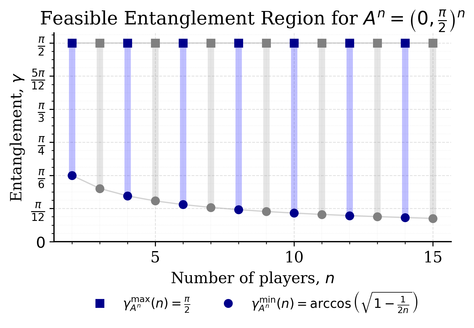
With this lower bound satisfied, the strategy profile $Q^{n}$ represents a Nash equilibrium for all $\Theta_{a}$ and $\Phi_{a}$. Because $\gamma\in[0,\frac{\pi}{2}]$, it is evident that $n\in[2,9]$, which is the range of $n$ for which Nash equilibria were known to exist in the case of maximal entanglement. Varying $\gamma$ does not allow for the formulation of novel Nash equilibria outside of this pre-established range. This is illustrated in Fig. 1. Interestingly, the possible values of $\gamma$ decrease as the number of players increases. This is also shown in the figure, where the feasible region, which represents acceptable values of $\gamma$ that preserve Nash equilibrium, shrinks as $n$ increases. Remarkably, Nash equilibrium is achieved in the case of three players with slightly less than a $\gamma=\frac{\pi}{4}$ level of entanglement in the system. These findings show that maximal entanglement is not required to realize symmetric Nash equilibria in the $Q^{n}$ strategy profile.

To determine the payoff of each player for the $A^{n}$ strategy profile, we refer to the evaluation of $c_{\theta,\phi}(x)$ and $s_{\theta,\phi}(x)$ in Eq. (53) and Eq. (54) of Koh, Kumar, and Goh’s work [41]. In Appendix E, we evaluate $w_{\theta,\phi}(x)$ in a similar way to get

	$\displaystyle c_{A^{n}}(x)$	$\displaystyle=(-1)^{\frac{n}{2}}[n\text{ even}][x=1^{n}],$
	$\displaystyle s_{A^{n}}(x)$	$\displaystyle=(-1)^{\frac{n-1}{2}}[n\text{ odd}][x=0^{n}],$
	$\displaystyle w_{A^{n}}(x)$	$\displaystyle=(-1)^{\frac{n-1}{2}}[n\text{ odd}][x=1^{n}].$		(29)

We now apply these to Eq. (15) and call it $p^{\gamma}_{A^{n}}(x)$. There are two cases to consider.

References

- Horodecki et al. [2009] R. Horodecki, P. Horodecki, M. Horodecki, and K. Horodecki, Quantum entanglement, Rev. Mod. Phys. 81, 865 (2009).
- Ekert and Jozsa [1998] A. Ekert and R. Jozsa, Quantum algorithms: entanglement–enhanced information processing, Philosophical Transactions of the Royal Society A: Mathematical, Physical and Engineering Sciences 356, 1769 (1998).
- Jozsa and Linden [2003] R. Jozsa and N. Linden, On the role of entanglement in quantum-computational speed-up, Proceedings of the Royal Society A: Mathematical, Physical and Engineering Sciences 459, 2011 (2003).
- Bruß and Macchiavello [2011] D. Bruß and C. Macchiavello, Multipartite entanglement in quantum algorithms, Phys. Rev. A 83, 052313 (2011).
- Biamonte et al. [2020] J. D. Biamonte, M. E. S. Morales, and D. E. Koh, Entanglement scaling in quantum advantage benchmarks, Phys. Rev. A 101, 012349 (2020).
- Díez-Valle et al. [2021] P. Díez-Valle, D. Porras, and J. J. García-Ripoll, Quantum variational optimization: The role of entanglement and problem hardness, Phys. Rev. A 104, 062426 (2021).
- You et al. [2021] J.-B. You, D. E. Koh, J. F. Kong, W.-J. Ding, C. E. Png, and L. Wu, Exploring variational quantum eigensolver ansatzes for the long-range XY model, arXiv preprint arXiv:2109.00288 (2021).
- Katabarwa et al. [2022] A. Katabarwa, S. Sim, D. E. Koh, and P.-L. Dallaire-Demers, Connecting geometry and performance of two-qubit parameterized quantum circuits, Quantum 6, 782 (2022).
- Horodecki et al. [2001] M. Horodecki, P. Horodecki, and R. Horodecki, Mixed-state entanglement and quantum communication, in Quantum Information: An Introduction to Basic Theoretical Concepts and Experiments (Springer Berlin Heidelberg, Berlin, Heidelberg, 2001) pp. 151–195.
- Ursin et al. [2007] R. Ursin, F. Tiefenbacher, T. Schmitt-Manderbach, H. Weier, T. Scheidl, M. Lindenthal, B. Blauensteiner, T. Jennewein, J. Perdigues, P. Trojek, B. Ömer, M. Fürst, M. Meyenburg, J. Rarity, Z. Sodnik, C. Barbieri, H. Weinfurter, and A. Zeilinger, Entanglement-based quantum communication over 144 km, Nature Physics 3, 481 (2007).
- Zou [2021] N. Zou, Quantum entanglement and its application in quantum communication, Journal of Physics: Conference Series 1827, 012120 (2021).
- Xing et al. [2023] J. Xing, T. Feng, Z. Fan, H. Ma, K. Bharti, D. E. Koh, and Y. Xiao, Fundamental limitations on communication over a quantum network, arXiv preprint arXiv:2306.04983 (2023).
- Xing et al. [2024] J. Xing, Y. Li, D. Qu, L. Xiao, Z. Fan, H. Ma, P. Xue, K. Bharti, D. E. Koh, and Y. Xiao, Teleportation with embezzling catalysts, Communications Physics 7, 357 (2024).
- Ekert [1991] A. K. Ekert, Quantum cryptography based on Bell’s theorem, Phys. Rev. Lett. 67, 661 (1991).
- Jennewein et al. [2000] T. Jennewein, C. Simon, G. Weihs, H. Weinfurter, and A. Zeilinger, Quantum cryptography with entangled photons, Phys. Rev. Lett. 84, 4729 (2000).
- Yin et al. [2020] J. Yin, Y.-H. Li, S.-K. Liao, M. Yang, Y. Cao, L. Zhang, J.-G. Ren, W.-Q. Cai, W.-Y. Liu, S.-L. Li, R. Shu, Y.-M. Huang, L. Deng, L. Li, Q. Zhang, N.-L. Liu, Y.-A. Chen, C.-Y. Lu, X.-B. Wang, F. Xu, J.-Y. Wang, C.-Z. Peng, A. K. Ekert, and J.-W. Pan, Entanglement-based secure quantum cryptography over 1,120 kilometres, Nature 582, 501 (2020).
- Giovannetti et al. [2011] V. Giovannetti, S. Lloyd, and L. Maccone, Advances in quantum metrology, Nature Photonics 5, 222 (2011).
- Huang et al. [2016] Z. Huang, C. Macchiavello, and L. Maccone, Usefulness of entanglement-assisted quantum metrology, Phys. Rev. A 94, 012101 (2016).
- Augusiak et al. [2016] R. Augusiak, J. Kołodyński, A. Streltsov, M. N. Bera, A. Acín, and M. Lewenstein, Asymptotic role of entanglement in quantum metrology, Phys. Rev. A 94, 012339 (2016).
- Eisert et al. [1999] J. Eisert, M. Wilkens, and M. Lewenstein, Quantum games and quantum strategies, Physical Review Letters 83, 3077 (1999).
- Eisert and Wilkens [2000] J. Eisert and M. Wilkens, Quantum games, Journal of Modern Optics 47, 2543 (2000).
- Flitney and Abbott [2002] A. P. Flitney and D. Abbott, An introduction to quantum game theory, Fluctuation and Noise Letters 2, R175 (2002).
- Khan et al. [2018] F. S. Khan, N. Solmeyer, R. Balu, and T. S. Humble, Quantum games: a review of the history, current state, and interpretation, Quantum Information Processing 17, 309 (2018).
- Meyer [1999] D. A. Meyer, Quantum strategies, Physical Review Letters 82, 1052 (1999).
- Benjamin and Hayden [2001] S. C. Benjamin and P. M. Hayden, Multiplayer quantum games, Phys. Rev. A 64, 030301(R) (2001).
- Tsakiroglou et al. [2026] M. Tsakiroglou, I. Liliopoulos, G. D. Varsamis, K. Milchanowski, and I. G. Karafyllidis, Graph-encoded strategic interactions in multiplayer quantum games, Quantum Information Processing 25, 109 (2026).
- Essalmi et al. [2026] K. Essalmi, F. Garrido, and F. Nashashibi, Multi-player, multi-strategy quantum game model for interaction-aware decision-making in autonomous driving, arXiv preprint arXiv:2602.03571 (2026).
- Li et al. [2002] H. Li, J. Du, and S. Massar, Continuous-variable quantum games, Physics Letters A 306, 73 (2002).
- Kay et al. [2001] R. Kay, N. F. Johnson, and S. C. Benjamin, Evolutionary quantum game, Journal of Physics A: Mathematical and General 34, L547 (2001).
- Sanz-Martín et al. [2025] L. Sanz-Martín, G. Rivas, N. Clavijo-Buriticá, M. Herrera, and J. Parra-Domínguez, Mapping the frontier: a review of quantum and evolutionary game theory for complex decision-making, Quantum Information Processing 24, 291 (2025).
- Du et al. [2000] J. Du, X. Xu, H. Li, X. Zhou, and R. Han, Nash equilibrium in the quantum battle of sexes game, arXiv preprint quant-ph/0010050 (2000).
- Piotrowski and Sładkowski [2002] E. Piotrowski and J. Sładkowski, Quantum market games, Physica A: Statistical Mechanics and its Applications 312, 208 (2002).
- Chen et al. [2004] Q. Chen, Y. Wang, J.-T. Liu, and K.-L. Wang, N-player quantum minority game, Physics Letters A 327, 98 (2004).
- Nawaz and Toor [2004] A. Nawaz and A. Toor, Dilemma and quantum battle of sexes, Journal of Physics A: Mathematical and General 37, 4437 (2004).
- Frąckiewicz [2009] P. Frąckiewicz, The ultimate solution to the quantum battle of the sexes game, Journal of Physics A: Mathematical and Theoretical 42, 365305 (2009).
- Consuelo-Leal et al. [2020] A. Consuelo-Leal, A. G. Araujo-Ferreira, E. Lucas-Oliveira, T. J. Bonagamba, and R. Auccaise, Pareto-optimal solution for the quantum battle of the sexes, Quantum Information Processing 19, 41 (2020).
- Szopa [2021] M. Szopa, Efficiency of classical and quantum games equilibria, Entropy 23, 506 (2021).
- Kastampolidou and Andronikos [2023] K. Kastampolidou and T. Andronikos, Quantum tapsilou—a quantum game inspired by the traditional greek coin tossing game tapsilou, Games 14, 72 (2023).
- Frąckiewicz and Szopa [2024] P. Frąckiewicz and M. Szopa, Permissible extensions of classical to quantum games combining three strategies, Quantum Information Processing 23, 75 (2024).
- Frąckiewicz et al. [2025] P. Frąckiewicz, A. Gorczyca-Goraj, and M. Szopa, Permissible four-strategy quantum extensions of classical games, Quantum Information Processing 24, 201 (2025).
- Koh et al. [2025] D. E. Koh, K. Kumar, and S. T. Goh, Quantum volunteer’s dilemma, Physical Review Research 7, 013104 (2025).
- Andronikos et al. [2025] T. Andronikos, C. Bitsakos, K. Nikas, G. I. Goumas, and N. Koziris, A GHZ-based protocol for the dining information brokers problem, Future Internet 17, 408 (2025).
- Essalmi et al. [2025] K. Essalmi, F. Garrido, and F. Nashashibi, Quantum game models for interaction-aware decision-making in automated driving, in 2025 IEEE International Conference on Advanced Robotics (ICAR) (2025) pp. 155–162.
- Smoliński et al. [2026] R. Smoliński, P. Frąckiewicz, K. Grzanka, and M. Szopa, Quantum negotiation games: Toward ethical equilibria, Entropy 28, 51 (2026).
- Vlachos and Karafyllidis [2009] P. Vlachos and I. G. Karafyllidis, Quantum game simulator, using the circuit model of quantum computation, Computer Physics Communications 180, 1990 (2009).
- Kotara et al. [2023] P. Kotara, T. Zawadzki, and K. Rycerz, Software aided analysis of EWL based quantum games, in Parallel Processing and Applied Mathematics, edited by R. Wyrzykowski, J. Dongarra, E. Deelman, and K. Karczewski (Springer International Publishing, Cham, 2023) pp. 209–220.
- Grzanka et al. [2025] K. Grzanka, A. Gorczyca-Goraj, M. Szopa, et al., QEGS: A Mathematica package for the analysis of quantum extended games, arXiv preprint arXiv:2505.00714 (2025).
- Johnson [2001] N. F. Johnson, Playing a quantum game with a corrupted source, Phys. Rev. A 63, 020302(R) (2001).
- Chen et al. [2003] L. Chen, H. Ang, D. Kiang, L. Kwek, and C. Lo, Quantum prisoner dilemma under decoherence, Physics Letters A 316, 317 (2003).
- Flitney and Abbott [2004] A. P. Flitney and D. Abbott, Quantum games with decoherence, Journal of Physics A: Mathematical and General 38, 449 (2004).
- Shuai et al. [2007] C. Shuai, F. Mao-Fa, and Z. Xiao-Juan, The effect of quantum noise on multiplayer quantum game, Chinese Physics 16, 915 (2007).
- Huang and Qiu [2016] Z. Huang and D. Qiu, Quantum games under decoherence, International Journal of Theoretical Physics 55, 965 (2016).
- Khan and Alam [2018] S. Khan and S. Alam, The dynamics of Nash equilibrium under non-Markovian classical noise in quantum prisoners’ dilemma, Reports on Mathematical Physics 81, 399 (2018).
- Kairon et al. [2020] P. Kairon, K. Thapliyal, R. Srikanth, and A. Pathak, Noisy three-player dilemma game: robustness of the quantum advantage, Quantum information processing 19, 327 (2020).
- Legón and Medina [2023] A. R. Legón and E. Medina, Joint probabilities approach to quantum games with noise, Entropy 25, 1222 (2023).
- Makram-Allah et al. [2026] A. T. M. Makram-Allah, M. Y. Abd-Rabbou, and N. Metwally, The possibility of fairly mitigating penalties in the quantum prisoner’s dilemma via classical noise channels, The European Physical Journal Plus 141, 456 (2026).
- Lu et al. [2004] J. Lu, L. Zhou, and L.-M. Kuang, Linear optics implementation for quantum game with two players, Physics Letters A 330, 48 (2004).
- Buluta et al. [2006] I. M. Buluta, S. Fujiwara, and S. Hasegawa, Quantum games in ion traps, Physics Letters A 358, 100 (2006).
- Mitra et al. [2007] A. Mitra, K. Sivapriya, and A. Kumar, Experimental implementation of a three qubit quantum game with corrupt source using nuclear magnetic resonance quantum information processor, Journal of Magnetic Resonance 187, 306 (2007).
- Prevedel et al. [2007] R. Prevedel, A. Stefanov, P. Walther, and A. Zeilinger, Experimental realization of a quantum game on a one-way quantum computer, New Journal of Physics 9, 205 (2007).
- Schmid et al. [2010] C. Schmid, A. P. Flitney, W. Wieczorek, N. Kiesel, H. Weinfurter, and L. C. Hollenberg, Experimental implementation of a four-player quantum game, New Journal of Physics 12, 063031 (2010).
- Xu and Wu [2022] K. Xu and Z. Wu, Experimental implementation of quantum prisoner dilemma on IBM quantum computers, in 2022 15th International Conference on Advanced Computer Theory and Engineering (ICACTE) (IEEE, 2022) pp. 13–18.
- Agreda et al. [2025] G. D. Agreda, C. A. D. Paredes, M. B. Samboni, J. A. Andrade, and S. C. Ordoñez, Bridging theory and practice in quantum game theory: Optimized implementation of the battle of the sexes with error mitigation on NISQ hardware, in 2025 IEEE CHILEAN Conference on Electrical, Electronics Engineering, Information and Communication Technologies (CHILECON) (2025) pp. 1–10.
- Agreda et al. [2026] G. D. D. Agreda, J. A. A. Hoyos, C. A. D. Paredes, S. C. Ordoñez, N. D. Hebdon, S. T. Goh, and D. E. Koh, Experimental implementation of the quantum volunteer’s dilemma on NISQ hardware: Noise analysis and digital-twin validation, arXiv preprint arXiv:2605.30676 (2026).
- Du et al. [2001] J. Du, X. Xu, H. Li, X. Zhou, and R. Han, Entanglement playing a dominating role in quantum games, Physics Letters A 289, 9 (2001).
- Du et al. [2002] J. Du, H. Li, X. Xu, X. Zhou, and R. Han, Entanglement enhanced multiplayer quantum games, Physics Letters A 302, 229 (2002).
- Özdemir et al. [2007] S. K. Özdemir, J. Shimamura, and N. Imoto, A necessary and sufficient condition to play games in quantum mechanical settings, New Journal of Physics 9, 43 (2007).
- Nawaz and Toor [2010] A. Nawaz and A. Toor, Quantum games and quantum discord, arXiv preprint arXiv:1012.1428 (2010).
- Ahmad [2013] N. Ahmad, The strategic form of quantum prisoners’ dilemma, Chinese Physics Letters 30, 050302 (2013).
- Li and Yong [2014] A. Li and X. Yong, Entanglement guarantees emergence of cooperation in quantum prisoner’s dilemma games on networks, Scientific Reports 4, 6286 (2014).
- Wei and Zhang [2017] Z. Wei and S. Zhang, Quantum game players can have advantage without discord, Information and Computation 256, 174 (2017).
- Santos [2019] A. C. Santos, Entanglement and coherence in quantum prisoner’s dilemma, Quantum Information Processing 19, 13 (2019).
- Mohamed et al. [2023] N. M. A. A. Mohamed, H. Taisheng, and P. Jinhui, Quantum game theory on entangled players, in International Conference on Intelligent Information Technologies for Industry (Springer, 2023) pp. 291–301.
- Bugu [2025] S. Bugu, Entanglement as a strategic resource in adversarial quantum games, arXiv preprint arXiv:2510.22444 (2025).
- Varsamis et al. [2025] G. D. Varsamis, I. Liliopoulos, H. Mohammadbagherpoor, A. K. Kostopoulos, K. Milchanowski, E. T. Karamatskos, P. Dimitrakis, R. P. Padbury, and I. G. Karafyllidis, Analysis of the effect of entanglement operators and the scalability of players’ payoff computation in n-player quantum games, Advanced Quantum Technologies 8, e00375 (2025).
- Diekmann [1985] A. Diekmann, Volunteer’s dilemma, Journal of Conflict Resolution 29, 605 (1985).
- Smith et al. [2016] J. E. Smith, S. Gavrilets, M. B. Mulder, P. L. Hooper, C. E. Mouden, D. Nettle, C. Hauert, K. Hill, S. Perry, A. E. Pusey, M. van Vugt, and E. A. Smith, Leadership in mammalian societies: Emergence, distribution, power, and payoff, Trends in Ecology & Evolution 31, 54 (2016).
- Weesie and Franzen [1998] J. Weesie and A. Franzen, Cost sharing in a volunteer’s dilemma, Journal of Conflict Resolution 42, 600 (1998).
- Otsubo and Rapoport [2008] H. Otsubo and A. Rapoport, Dynamic volunteer’s dilemmas over a finite horizon: An experimental study, Journal of Conflict Resolution 52, 961 (2008).
- Latané and Darley [1970] B. Latané and J. M. Darley, The Unresponsive Bystander: Why Doesn’t He Help? (Appleton-Century-Crofts, New York, 1970).
- Campos-Mercade [2021] P. Campos-Mercade, The volunteer’s dilemma explains the bystander effect, Journal of Economic Behavior & Organization 186, 646 (2021).
- Darley and Latané [1968] J. M. Darley and B. Latané, Bystander intervention in emergencies: Diffusion of responsibility, Journal of Personality and Social Psychology 8, 377 (1968).
- Barron and Yechiam [2002] G. Barron and E. Yechiam, Private e-mail requests and the diffusion of responsibility, Computers in Human Behavior 18, 507 (2002).
- Battaglini and Palfrey [2025] M. Battaglini and T. R. Palfrey, Welfare in the volunteer’s dilemma, Journal of Public Economics 245, 105360 (2025).
- Hilbe et al. [2014] C. Hilbe, B. Wu, A. Traulsen, and M. A. Nowak, Cooperation and control in multiplayer social dilemmas, Proceedings of the National Academy of Sciences of the United States of America 111, 16425 (2014).
- Amir et al. [2026a] R. Amir, D. Machowska, and J. Tian, The volunteer’s dilemma with cost synergies, Journal of Conflict Resolution 70, 1095 (2026a).
- Searcy and Nowicki [2010] W. A. Searcy and S. Nowicki, The evolution of animal communication: reliability and deception in signaling systems (Princeton University Press, 2010).
- Mielke et al. [2019] A. Mielke, C. Crockford, and R. M. Wittig, Snake alarm calls as a public good in sooty mangabeys, Animal Behaviour 158, 201 (2019).
- Steinegger et al. [2020] M. Steinegger, H. Sarhan, and R. Bshary, Laboratory experiments reveal effects of group size on hunting performance in yellow saddle goatfish, parupeneus cyclostomus, Animal Behaviour 168, 159 (2020).
- Heifetz et al. [2021] A. Heifetz, R. Heller, and R. Ostreiher, Do Arabian babblers play mixed strategies in a “volunteer’s dilemma”?, Journal of Behavioral and Experimental Economics 91, 101661 (2021).
- Padget et al. [2026] R. F. B. Padget, F. J. Thompson, R. A. Johnstone, M. A. Cant, and B. Kuijper, Sharing the cost? Soldier investment following colony fusion in basal termites, Insectes Sociaux 10.1007/s00040-026-01105-w (2026).
- Morsky and Vural [2018] B. Morsky and D. C. Vural, Cheater-altruist synergy in public goods games, Journal of Theoretical Biology 454, 231 (2018).
- Archetti and Pienta [2019] M. Archetti and K. J. Pienta, Cooperation among cancer cells: applying game theory to cancer, Nature Reviews Cancer 19, 110 (2019).
- Manini and López [2022] C. Manini and J. I. López, Ecology and games in cancer: new insights into the disease, Pathologica 114, 347 (2022).
- Pedroso [2018] M. Pedroso, The impact of population bottlenecks on the social lives of microbes, Biological Theory 13, 190 (2018).
- Patel et al. [2019] M. Patel, B. Raymond, M. B. Bonsall, and S. A. West, Crystal toxins and the volunteer’s dilemma in bacteria, Journal of Evolutionary Biology 32, 310 (2019).
- Diekmann [1993] A. Diekmann, Cooperation in an asymmetric volunteer’s dilemma game theory and experimental evidence, International Journal of Game Theory 22, 75 (1993).
- Weesie [1993] J. Weesie, Asymmetry and timing in the volunteer’s dilemma, Journal of conflict resolution 37, 569 (1993).
- He et al. [2014] J.-Z. He, R.-W. Wang, and Y.-T. Li, Evolutionary stability in the asymmetric volunteer’s dilemma, PloS one 9, e103931 (2014).
- Healy and Pate [2018] A. J. Healy and J. G. Pate, Cost asymmetry and incomplete information in a volunteer’s dilemma experiment, Social Choice and Welfare 51, 465 (2018).
- Guo et al. [2023] Z.-X. Guo, J.-Z. He, Q.-M. Li, L. Shi, and R.-W. Wang, Asymmetric interaction and diverse forms in public goods production in volunteer dilemma game, Chaos, Solitons & Fractals 166, 112928 (2023).
- Chen et al. [2013] X. Chen, T. Gross, and U. Dieckmann, Shared rewarding overcomes defection traps in generalized volunteer’s dilemmas, Journal of theoretical biology 335, 13 (2013).
- Mago and Pate [2023] S. D. Mago and J. Pate, Greed and fear: Competitive and charitable priming in a threshold volunteer’s dilemma, Economic Inquiry 61, 138 (2023).
- Weesie [1994] J. Weesie, Incomplete information and timing in the volunteer’s dilemma: A comparison of four models, Journal of Conflict Resolution 38, 557 (1994).
- Amir et al. [2026b] R. Amir, H. Liu, T. Mayskaya, and J. Tian, On the repeated volunteer’s dilemma with equal cost sharing, Available at SSRN 5634211 10.2139/ssrn.5634211 (2026b).
- Nash Jr. [1951] J. F. Nash Jr., Non-cooperative games, Annals of Mathematics 54, 286 (1951).
- Cheng et al. [2023] B. Cheng, X.-H. Deng, X. Gu, Y. He, G. Hu, P. Huang, J. Li, B.-C. Lin, D. Lu, Y. Lu, C. Qiu, H. Wang, T. Xin, S. Yu, M.-H. Yung, J. Zeng, S. Zhang, Y. Zhong, X. Peng, F. Nori, and D. Yu, Noisy intermediate-scale quantum computers, Frontiers of Physics 18, 21308 (2023).