Stochastic scalar-tensor inflation and beyond
Abstract
During cosmological inflation, inhomogeneities arising from quantum vacuum fluctuations are stretched to become super-Hubble and effectively classical. As many scenarios of the origin involve nonlinearities or a breakdown of perturbativity in the infrared, the limitations of quantum field theory can be addressed using a stochastic description of the dynamics, the so-called stochastic inflation paradigm. However, the stochastic formalism was only recently formulated consistently within full General Relativity and has not yet been extended to more general theories of the early universe, which is the subject of this work.
In order to find the stochastic sources for a wide class of fully nonlinear scalar-tensor theories, we apply our gauge-agnostic coarse-graining procedure to the linear equations of the effective field theory of dark energy. Each theory can then be mapped to its own set of stochastic equations of motion by identifying the corresponding coefficients in the EFT. We illustrate this with a few concrete and, in most cases, unprecedented examples, including Gauss-Bonnet, generalized Brans-Dicke, Horndeski, and braiding theories.
Finally, we discuss other natural extensions to provide a phenomenologically complete stochastic framework. For example, we showcase the coarse-graining of multifield inflation in full General Relativity and argue for the generality of our procedure and thus its potential applications beyond the realm of inflation.
1 Introduction
Inflation is the most widely accepted formalism for the description of the early universe [starobinsky80, guth_1981, Linde82], providing a compelling explanation for the observed homogeneity, isotropy, and flatness of the cosmos, as well as a mechanism for generating the primordial density perturbations that seeded the formation of large-scale structure [Mukhanov1981, Hawking1982, Starobinsky1982pert, Guth82pert, HawkingMoss1982, Bardeen83]. However, the dynamics of inflation in this framework are believed to be inherently quantum mechanical from the vacuum fluctuations of the inflaton field, and are still an active area of research, with, as mentioned below, many remaining open questions and challenges.
Stochastic Inflation, born not so long after Inflation [Starobinsky_stochastic_1988], has proved itself as the main complementary method to the standard quantum field theoretic approaches in the prediction of observables. As it is possible to observe the breaking of perturbativity in some scenarios, stochastic inflation makes the most of the seemingly coincidental classicality there to provide a nonperturbative model of the dynamics, semiclassically sourced by the quantum vacuum fluctuations’ noise. Since its early days [Starobinsky_stochastic_1988, salopek_nonlinear_1990, salopek_stochastic_1991, rigopoulos_non-linear_2005, vennin_correlation_2015-1], Stochastic Inflation has been used in the long wavelength limit of General Relativity (GR), yielding numerous developments and predictions on classicalised primordial perturbations [nakao_stochastic_1988, nambu_stochastic_1988, sasaki_classical_1988, hosoya_stochastic_1989, habib_stochastic_1992, bellini_stochastic_1996, Winitzki00, rigopoulos_separate_2003, liguori_stochastic_2004, tsamis_stochastic_2005, Rigopoulos_multi06, BattefeldVanTent06, tolley_stochastic_2008, gratton_path_2011, Fujita2013, levasseur_lagrangian_2013, levasseur_recursive_2013, rigopoulos_fluctuation-dissipation_2013, garbrecht_infrared_2014, burgess_eft_2015, levasseur_backreaction_2015, assadullahi_multiple_2016, burgess_open_2016, grain_stochastic_2017, pattison_quantum_2017, vennin_critical_2017, prokopec_functional_2018, pattison_attractive_2018, noorbala_tunneling_2018, markkanen_scalar_2019, pinol_inflationary_2019, firouzjahi_stochastic_2019, pattison_stochastic_2019, ezquiaga_exponential_2020, Bounakis20, de_numerically_2020, pattison_ultra-slow-roll_2021, ando_power_2021, cohen_stochastic_2021, cable_free_2021, prokopec_ensuremathdeltan_2021, Jackson22, tasinato_stochastic_2022, Figueroa22, tada_statistics_2022, cable_second-order_2022, cruces_stochastic_2022, mishra_primordial_2023, wilkins_stochastic_2023, tomberg_numerical_2023, Tomberg:2024evi, mizuguchi_stolas_2024, tajima_stochastic_2024, cruces_small_2024, jackson_stochastic_2024, tomberg_ito_2024, ballesteros_non-gaussian_2024, noorbala_classicality_2024, sharma_stochastic_2024, Animali25, tasinato_stochastic_2025, nassiri-rad_stochastic_2025, miyamoto_calculating_2025, briaud_stochastic_2025, blachier_friction_2025, barenboim_large_2025, murata_stochastic_2026, saha_nonlinear_2026, beneke_quantum_2026, ye_nonperturbative_2026, cruces_consistent_2026, mishra_eigenvalue_2026, animali_time-reversed_2026, Li26b]. Some of these refinements of Starobinsky’s original idea over the years have arised to describe more and more regimes. In particular, many works explored the breaking of perturbativity beyond secular growth arising on fixed dS backgrounds. In general with a full spacetime, whether a theory can produce such secular effects or not [Assassi12] not does not protect from nonperturbative dynamics. For instance, models of ultra-slow-roll phases of inflation have attracted significant interests in their promise to produce strong overdensities and subsequent primordial black holes.
Among others, such models and methods have also shown some challenges given the subtleties and debates in the full account of gradients, rightful gauges, backreaction etc, see for instance [artigas_hamiltonian_2022, Artigas25, jackson23]. Recent work [Launay24] shows that, if one is ready to give up analytical solutions, it is possible to build such a formalism in full general relativity, and to solve it numerically [Launay26], without having to think about the validity of many historical approximations apart from classicality (see [Launay2024bis] on the matter). The procedure employed there is deeply rooted in the mastery of linear perturbation theory in any gauge, and, as conveyed in this work, can be extended beyond single scalar-field inflation in GR.
With the same minimal approximations, this work provides the generalisation of stochastic inflation to scalar-tensor theories going beyond General Relativity. These theories constitute in fact the generic extension of GR with a scalar degree of freedom relevant for inflation and, more generally, dark energy, and encompass a wide class of viable inflationary frameworks while remaining theoretically controlled. In the perturbative limit —useful to derive stochastic sources as we will recall— these theories are easierly gathered in the same formalism using the Effective Field Theory of Inflation (EFToI), as a special case of the EFT of dark energy (EFToDE). Initially sparkling from the EFToI, the latter formalism reached great maturity in the past two decades, as part of an effort to constrain post-inflation dark energy models, and even rule out some of these for late eras of cosmology [CreminelliVernizzi17]. As we will see, the associated notations, in particular those of the so-called basis [BelliniSawicki14], are still particularly meaningful for the study of inflation. The EFToI is today a subset of this scalar-tensor framework, and usually goes further in its approximations. In particular, mixings with gravity are usually neglected by assuming that the Hubble parameter, or the energy, is above the decoupling scale (equivalent in practice to , and , at fixed ). In the first place, these energies are much higher than the late-time ones but the freezing of the gauge-invariant fluctuations at Hubble scale crossing makes the imprint at those energies relevant. The predictability of such approach has recently culminated thanks to perturbative solvers such as CosmoFlow [werth23].
For the case of inflation and before even mentioning nonperturbative effects, the perturbative approach is not without generalisations and motivations beyond the decoupling limit. In particular, computations of the curvature perturbation 3-point function —as the leading signal of inflationary interactions— have been performed beyond this limit. The pioneering work of Maldacena [Maldacena_2003] gave early on the 3-point function of the curvature perturbation in single-field slow-roll inflation with the mixings with metric perturbations and the leading slow-roll contributions in General Relativity. This was later extended to more general single-field actions11 1 As well as various multifield extensions, including the decoupled EFToI treatment of [senatore_effective_2012]., such as those with single-field non-canonical kinetic terms [seery_primordial_2005, chen_primordial_2010, burrage_large_2011], including braiding [zhang_primordial_2021], but also various calculations in the general Horndeski classes with those mixings involved [de_felice_inflationary_2011, felice_primordial_2011], including the gravitonic bispectra [gao_primordial_2011]. To make such tedious calculations accessible in non-decoupled regimes, numerical pipelines such as [Zhang25] have also been developed. Importantly, these works emphasise that nontrivial contributions can be found and be missed by the decoupling limit in a generic scalar-tensor theory. Moreover, even if GR or the decoupling limit are found to be good approximations to certain energy scales, such extended treatments are necessary to quantify the validity of the former. It is also worth mentioning that a plethora of inflationary models formulated in GR, whether given as interactive actions or simple potentials (e.g. the widespread scalaron Starobinsky model [StarobinskyScalaron1980]), have been derived from scalar-tensor theories using transformations to the so-called Einstein frame. However such transformations between frames do not always exist [Zumalacarregui13] or could generate increased complexity beyond the single-field scenario, as a field space curvature might be generated in the multifield case [Kaiser10].
In the aforementioned existing calculations, beyond the decoupling limit or not, several approximations are employed on top of perturbativity and the tree-level limitation22 2 Loop calculations are still challenging today [Senatore10, Assassi12, lee_leading_23] and are thus not part of any numerical pipeline., such as the freezing of couplings at the horizon or perturbative expansions on state properties or couplings (including sound speed, slow-roll parameters etc). More generally, computations of correlators —even at tree-level— have never been implemented for a generic scalar-tensor theory, whether using in-in integrations or abovementioned transport equations. In this context, one can see that the fully quantum methods are not only unable to handle nonperturbative dynamics at the moment, but also to handle systematically the full variety of perturbative and nonlinear dynamics in the landscape of inflationary models.
At the expense of analytic work and most importantly quantum effects, relying on evolving the equations of motion is usually the easiest way to resolve full nonlinearities and nonperturbative effects, as shown by multiple works in the context of inflation [Cosmolattice, latticeeasy, clough_robustness_2017, Elley2024, Caravano22thesis, Launay2025, Giannadakis25]. However, the stochastic approach is precisely restricted to a semiclassical regime, and so, it is not a problem to give up the offshell part of the system’s description, as long as the classicality condition is satisfied. Providing a theory of stochastic inflation in a generic scalar-tensor theory is thus about providing a simpler, if not first, access to correlators from generic theories of the origin by exploiting the semiclassicality of the inflationary spacetime.
This paper is organised as follows. The general philosophy and procedure to build stochastic equations from an IR theory is briefly introduced in Section 2.1. In order to derive the stochastic sources of generic scalar-tensor theories via their linear equations without applying the coarse-graining to each theory separately, we introduce the EFToDE and our chosen notations in Section 2.2. The stochastic ansatz is then applied to get our main result summarised in Section 2.4.3: the stochastic sources of the scalar-tensor equations of motion of theories admitting a decomposition in the EFToDE when linearised. In Section , we put this result into practice for a variety of theories. This means finding the EFToDE coefficients that each chosen theory corresponds to, including nonminimally coupled theories, Einstein-Gauss-Bonnet, Horndeski, Braiding, before applying the main result. Finally, Section concludes by pushing the stochastic ansatz to its edge discussing further possible extensions, inspired by previous works and the generality of our EFToDE notations. For instance, we demonstrate the generality and naturalness of our advertised procedure by coarse-graining multifield GR for the first time.
Notations.
In the following, we will use the following tensor for comparison to the Einstein field equations,
with a potentially time-dependent Planck mass and the action of our theory. When is the Einstein-Hilbert action with some content described by a stress-energy tensor , we recover , with the Planck mass . vanishes in the least action configuration (on-shell). In full generality, we also define
useful for instance to look at scalar field equations of motion.
We will also use to denote the Fourier transform, and to denote the Fourier transform of a white noise, and usual notations of an FLRW spacetime with scale factor , Hubble rate , Hubble slow-roll parameters , being the cosmic time. Apart from which are implicitly background quantities, we will use the subscript to denote the background value of a field.
2 Scalar-tensor stochastic sources
2.1 Stochastic ansatz
Stochastic inflation33 3 I defer to [Starobinsky_stochastic_1988, vennin_correlation_2015, cruces_review_2022, Launay24] for further technical and state-of-the-art reviews. was originally designed to tackle the description of IR secular growth of perturbations of a inflaton in de Sitter [Starobinsky_stochastic_1988]. As IR modes were growing beyond the perturbativity bounds of QFT, it was convenient to observe the (nonperturbative-growth-friendly) classicality of each mode as the Hubble radius becomes smaller () during inflation. Concretely, commutators were found to be decaying from this time-dependent cutoff and quantum operators turned into stochastic numbers, with a quantum-originated spectrum. The stochastic ansatz is thus simply assuming that, statistics-wise, inhomogeneous inflation can be looked at using the classical open IR system of scales, described by stochastic PDEs44 4 In principle, this doesn’t require the noise to be originated from a quantum theory using quantum initial conditions.. Beyond that simple ansatz come further nuances in diverse treatments, see for instance historical approximations used in General Relativity [salopek_nonlinear_1990, salopek_stochastic_1991]. The common point of all stochastic equations of motion formulated so far for inflation, which could thus be appended to the stochastic ansatz, is the linear approximation for the UV quantum modes. In mathematical terms, focusing without loss of generality on a field , with decomposition between its IR classical and nonlinear part and its UV part , this can be written with a nonzero r.h.s.
| (2.1) | ||||
where is the original classical equation of motion applied to the IR field , and is the original linearised equation of motion applied to the UV field . The linear operator uses the average of the IR field as its background (Starobinsky approximation), or the IR field itself depending on the treatment of the stochastic backreaction. The separation has been made explicit using a window function selecting the IR modes, and . We wrote the approximation as an equality up to the term to emphasise that the linear operator is applied to the product of the UV window and the field, which will simplify dramatically this r.h.s.. In practice, the source is computed by solving in parallel for the spectrum of the noise using . In this manuscript, we refer to this whole algebraic procedure as the coarse-graining.
Rigourous derivations can be found in [morikawa_dissipation_1990, moss_effective_2017, pinol_manifestly_2021] using the Closed-Time-Path formalism and integrating out the UV modes, but we sketch here a simplistic proof for the reader. Let be an action of interest, functional of one field for simplicity.
We assume perturbativity in the UV field next, , and write the functional Taylor expansion of the action up to first order
| (2.2) |
This allows us to extract the equation of motion (EOM) of the IR field up to linear order in UV corrections
| (2.3) | ||||
after injecting the previous expansion. Using now the classicality assumption on , we can assume that the evolution is entirely described by
so that
| (2.4) |
This says that the classical EOM of the IR field is the same as that of the original EOM, supplemented by a right-hand side source fueled by the UV field. The double functional derivative applied to S is the inverse propagator, which is the linear equation of motion operator55 5 This is more subtle for the metric propagator and more generally when gauge d.o.f.s are involved..
This short demonstration appears heuristic for two reasons, which can be rigorously answered. First, is technically a quantum operator, however, the operator acting on it will only leave terms with a time derivative acting on the window after simplification of the linear EOM, meaning that the UV modes will only contribute at the time of crossing, where they are classicalised and can be treated as stochastic numbers with their quantum-originated spectrum. Second, the case of full GR and beyond is more subtle because of the gauge-dependence as pointed out in [Launay24]. The procedure used in the cited work and the present one successfully tackles that, as explained in Sections 2.3.3 and 2.4.
Note that this work does not look at the validity of the separation of linear quantum vs nonlinear classical scales, and as advocated in [Launay2024bis, Ballesteros26], assumes that every scenario of inflation and every set of scales selected by should have a classicality criterion checked using QFT-based arguments in their perturbative phase. Instead, this work leaves the choice of the window function unspecified and focuses on applying the stochastic ansatz described above to the most general variety of theories, without making any further approximation on the dynamics. Keeping those notations general will also be fruitful to discuss application beyond the standard case of inflation in Section .
In the following, we apply the stochastic ansatz to a wide class of theories dark energy beyond GR at the same time (i.e. not one by one specifically) by using an EFT description gathering all linear descriptions at once.
2.2 Primer on the EFT of Dark Energy
Given the linear origin of the sources, the EFT of Dark Energy is the ideal framework to describe the dynamics of the UV modes and compute the sources of all included theories simultaneously. It provides indeed a unified way to write down the most general action for a single scalar degree of freedom coupled to gravity, without having to specify the underlying theory. Later in Section , we will specify some of the EFT coefficients to match some known higher-order relativistic theories. The following subsections first introduce the reader to these tools and notations, mostly taken from [Gleyzes13, Gleyzes14].
2.2.1 Symmetries and actions
The Effective Field Theory of Dark Energy (EFToDE) is a powerful framework to describe the dynamics of dark energy and gravity. It is based on the idea that dark energy can be described as a low-energy effective theory, where the high-energy degrees of freedom are integrated out. This allows us to capture the essential features of dark energy without needing to specify its microscopic origin and so the fully nonlinear EOM. The action of the EFToDE is written in the unitary gauge as [Gleyzes13]
| (2.5) | ||||
where is the Planck mass, and are the -dimensional and -dimensional Ricci scalars respectively, and is the extrinsic curvature. Under this form, this is the most general action for a single scalar degree of freedom coupled to gravity, up to second order in perturbations and with at most two derivatives in the quadratic action. The first line is to be understood as the background action, while the second one represents the quadratic expansion around the FLRW metric. and play the role of the scalar potential and kinetic energy respectively, while the diverse time-dependent mass coefficients encode its self and metric interactions. In GR, the latter take the values and .
The least action principle yields the background equations of motion
| (2.6) | ||||
| (2.7) |
where is the Hubble rate and , are the dark energy energy density and pressure.
The EFToI is a special case of the EFToDE corresponding to a data-constrained background evolution. In GR inflation, this translates into having
| (2.8a) | ||||
| (2.8b) | ||||
where is the first Hubble slow-roll parameter, small enough for long enough to ensure a sufficient number of e-folds of inflation and a quasi-scale-invariant power spectrum of perturbations [PlanckInflation]. For the sake of generality, we will keep general notations.
At this stage, the action suffers from a broken time diffeomorphism invariance, which can be restored by introducing a scalar field that transforms under time diffeomorphisms. This scalar field can be thought of as the Goldstone boson associated with the breaking of time diffeomorphisms. By performing the Stueckelberg trick , we can restore the full diffeomorphism invariance of the theory and analyze the dynamics of perturbations gauge-agnostically. The procedure is rather involving as it also requires the modification of the space foliation used in the definition of the extrinsic curvature. This was performed in past work, including the specific but pioneering case of inflation [Cheung08]. For our purpose we will only need the entailed linearized equations of motion known from past works.
As this work is originally motivated for the study of the inflaton, it is worth mentioning that the EFToI predates its generalisation into EFToDE and usually takes a further step in the approximations by assuming the decoupling limit, which corresponds to neglecting the mixings with gravity and thus the metric perturbations. This is why a great part of the literature focuses on the interactions of alone but we do not make this approximation here, as we want to capture the full dynamics of the system, including the mixings with gravity, which can be important in some regimes touched by e.g. stochastic inflation.
For the purpose of generality and interpretability, we will stick to the EFToDE notations without assuming the inflationary limit unless specified otherwise.
2.2.2 An interpretable parametrisation
Rarely used in the context of inflation, another parametrisation of the quadratic terms in eqn. (2.5) is possible and more interpretable. The so-called -basis [BelliniSawicki14] uses five dimensionless and independent functions of time:
- •
: Kineticity, which quantifies the kinetic energy of the scalar field perturbations
- •
: Braiding, which describes the mixing between the scalar field and the metric perturbations
- •
: Tensor speed excess, which measures the deviation of the speed of gravitational waves from the speed of light
- •
: Planck-mass running rate, which quantifies the rate of change of the effective Planck mass with time
- •
: Horndeski Planck-mass running, which captures the time variation of the effective Planck mass in Horndeski theories. When set to zero, the action describes all Horndeski quadratic actions.
Analogously to the Hubble slow-roll parameters, we also introduce the notation
with for .
With this basis, the quadratic action reads [Gleyzes14]
| (2.9) | |||
where is the spatial metric, is the perturbation of the lapse function, and the running Planck mass relates to , and as
| (2.10a) | ||||
| (2.10b) | ||||
with other conversions from eqn. (2.5) to the -basis given in [Gleyzes14].
Setting and , gives back GR, while is the inflationary limit of the kineticity.
Note that one can also go beyond this framework and include beyond second order spatial or time derivatives, in the latter case as long as they do not give rise to Ostrogradsky instabilities and ghosts. We will comment on generalisation to those cases in Section .
2.3 Linear cosmology of the EFT of dark energy
Along the boson perturbation, we write the scalar perturbations of the metric with the following convention
| (2.11) | ||||
where the secundary notations are those of [Gleyzes13], and where we defined the operator and .
2.3.1 Gauge-agnostic equations
The linear equations of motion were derived in [Gleyzes13] in the Newtonian Gauge. We used those and recovered independently66 6 Note that Appendix D of [Gleyzes13] contains typos in the display: factor missing on the term of ; the simplification should yield as opposed to ; the term of the factor should be on not the basis linear equations, as displayed in [Gleyzes14] in this gauge for (up-down indices linear Einstein equations). For use in post-inflationary studies, the literature usually showcases either the Newtonian or the synchronous gauge equations. This work does not restric to such choice. It is possible to leave the Newtonian gauge for a gauge-agnostic treatment using the transformation
| (2.12) | ||||
where rehabilitates arbitrary and perturbations of the and metric components. If one is interested in the linear equations including the boson , performing the Stueckelberg trick at this stage is easier than in the EFT action. This transformation yields the following gauge-agnostic linear equations of motion and their constraints for the EFToDE in the basis
| (2.13a) | ||||
| (2.13b) | ||||
| (2.13c) | ||||
| (2.13d) | ||||
where we defined trace and traceless parts using the (transverse) projection operator
and the linear Einstein EOM lhs terms
| (2.14a) | ||||
| (2.14b) | ||||
| (2.14c) | ||||
| (2.14d) | ||||
Note that, by orthogonality, and are both null on-shell and the latter could be injected in the expression of the former in eqn. (2.14c). However, we keep it this way as the coarse-grained theory will not be on-shell, as explained in Section 2.1.
More involving, the linear EOM of is given by
| (2.15) |
We are not interested in the hydrodynamical equations, and so do not rewrite the evolution equation found in [Gleyzes13, Gleyzes14]. A related discussion on potential extensions is lead in Section . The same remark is valid for vector modes. Spin-2 linear equations are easier to write than the scalar ones as the gauge-invariance of the tensorial perturbations mean that the linear contribution to the Einstein equations is proportional to the polarised Mukhanov-Sasaki equations. We thus focus on scalars until Section 2.4.2 without loss of generality.
2.3.2 Curvature perturbation dynamics
Despite the complexity of eqn. (2.13) and (2.14), a single gauge-invariant perturbation can summarise the linear scalar dynamics, as we recall below using the curvature perturbation on comoving hypersurfaces
| (2.16) |
Mukhanov-Sasaki equation.
Define the field as
| (2.17) |
and the nonlinear combination . The logarithmic cosmic time derivative is
| (2.18) |
A cosmologist would notably find back the term of the GR Mukhanov-Sasaki equation in . Define now the sound speed
| (2.19) |
The Mukhanov-Sasaki equation can be found by rewriting the EFToDE action or the linear equations in the unitary gauge, giving [Gleyzes13]
| (2.20) |
For the case of inflation, and similarly to GR, these modes could be given Bunch-Davies initial conditions in the sub-Hubble regime. The value of a mode at (chosen) crossing to the IR has a direct impact on the amplitude of the stochastic sources. Let us look at its value in the case of inflation. By defining , we can rewrite eqn. (2.20) in conformal time as
| (2.21) |
and assume slowly-varying Hubble and EFT rolling parameters at crossing (), so that the solution is analytically known as
| (2.22) |
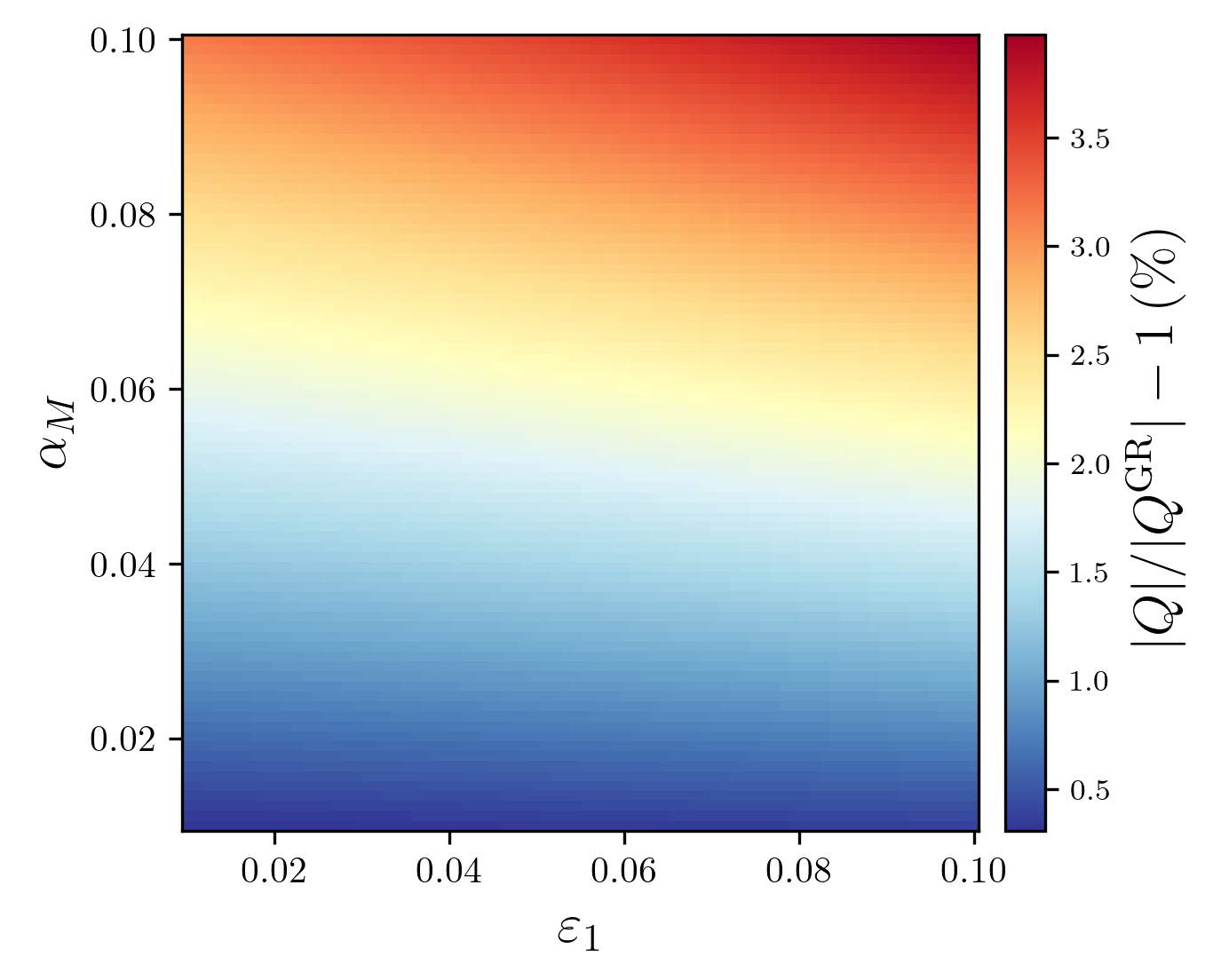
where , using Bunch-Davies initial conditions in the deep sub-Hubble regime. We provide a visual comparison of with and without running of the Planck mass in Figure 1. A few percents deviation can be reached with a reasonably perturbative value, translating in a similar difference per efold in the amplitude of the stochastics we are about to compute.
2.3.3 Perturbations as functionals of
Following the procedure developed in [Launay24] before performing the coarse-graining, we express the gauge invariant combinations in terms of . These are easily obtained in the comoving gauge where and where by definition.
In the comoving gauge the momentum constraint eqn. (2.13b) reduces to solving , giving
| (2.23) |
Substituting the above into the Hamiltonian constraint eqn. (2.13a) yields
| (2.24) |
which here equates . The energy density perturbation is found too as . We can now evaluate the common gauge invariants used in cosmology, as functionals of
| (2.25a) | ||||
| (2.25b) | ||||
| (2.25c) | ||||
| (2.25d) | ||||
where is the effective dark energy density plus pressure, and where we referred to the derived comoving gauge functionals we just derived explicitly. As shown in our previous work in GR for inflation [Launay24], knowing these as functionals of is particularly useful to get all gauges expressed as functionals of . In particular in the relevant gauges, this provides physically-motivated cosmological initial conditions for numerical relativity in modified gravity, without relying on arbitrary initial perturbations and constraint solvers.
Finally, one can compute the gravitational slip as
| (2.26a) | ||||
| (2.26b) | ||||
| (2.26c) | ||||
In the second line, we injected the Mukhanov-Sasaki equation, eqn. (2.20). In GR, this becomes clearly as expected, but not in the general case. In this study, it is important not to inject the Mukhanov-Sasaki equation in the expression of the gravitational slip or any EOMs before coarse-graining. In fact, the coarse-grained gravitational slip is non-zero, even in GR [Launay24].
2.4 Sources to all EOMs
Now that we have identified the true underlying dynamical field () in the EOMs, we have everything we need to proceed with the coarse-graining of the linear theory as described in Section 2.1.
2.4.1 Scalar sector
As explained in Section 2.1, the coarse-graining procedure consists in seeing the change of the linear equations of motion of a field under the transformation
| (2.27) |
where is a window function, before promoting the result to be the spectrum of the stochastic source to the nonlinear EOMs. However in full general relativity, and despite having a single scalar degree of freedom, multiple scalar perturbations are at play with no clear prescription for their coarse-graining as a group. Moreover, coarse-graining should not be gauge-dependent, and thus should be performed on gauge-invariant combinations of the fields, as we advocated in [Launay24]. This is why using the coarse-graining is the most natural choice, in particular after having expressed all the gauge-invariant combinations as functionals of in the previous section.
In fact, eqns. (2.25), allow us to write any field in any gauge as a functional of . If one picks a gauge-dependent perturbation without specifying its value in a given gauge, say , then all other gauge-dependent quantities can be expressed as functionals of and
| (2.28a) | ||||
| (2.28b) | ||||
| (2.28c) | ||||
Substituting these three functionals in the linear equations of motion, eqn. (2.13) and eqn. (2.13d), will simplify out and give the Mukhanov-sasaki equations up to different factors, except for the constraints which will be automatically satisfied by definition and as non-dynamical equations. As we are about to see, substituting the coarse-grained functionals however, might not give these results, as we are about to see.
Mukhanov-Sasaki equation.
Even as a linear EOM, the Mukhanov-Sasaki equation itself can be coarse-grained and will appear useful in the simplification of the sources to the full EOMs. In Fourier space, satisfies the following equation
| (2.29) |
after simplifying using the MS equation satisfied by so that the source Fourier amplitude takes the form
| (2.30) |
The result in canonical inflation GR of [Launay24], noted , is recovered in this limit where and . This is particularly visible when writing
| (2.31) |
with a function of the parameters that vanishes in the GR limit and defined as
| (2.32) |
Constraint IR equations.
We now plug the coarse-grained and gauge-agnostic perturbations functionals defined in the previous subsection, in the Hamiltonian and momentum constraints, eqn. (2.13a) and eqn. (2.13b), and call and the results in Fourier space, after simplifying using the MS equation satisfied by . We find that these source spectra obtained vanish perfectly
| (2.33) |
As shown in previous work [Launay24, Launay2025], this is the benefit of using the gauge-agnostic coarse-graining. We should stress again, that no previous work in the stochastic inflation literature, apart from [Launay24] and the present one, showed explicit satisfaction of the coarse-grained constraints, which is rather essential to input a physically-balanced stochastic kick at each time step. At best, the local Friedmann equation corresponding to the Hamiltonian in the separate universe approximation (0th order gradient expansion) would be enforced in most works, and the momentum equation has been used to prepare initial data at next order in the gradient expansion [prokopec_ensuremathdeltan_2021]. Some works, including in the context of higher curvature corrections, have found a non-zero source to the constraints (see eqns. (61) and (64) of [aldabergenov_towards_2025]). We believe and have seen in our own previous attempts that this might be a consequence of coarse-graining in a specific gauge inconsistently (flat gauge in the mentioned work) or simplifying with the MS equation before coarse-graining.
Source to IR Dark Energy.
Leaving the constraints and the MS equation yields much more complexity at first sight as we get the source Fourier amplitude for eqn. (2.13d) to be, after substituting the functionals of and , simplifying and the MS equation in ,
| (2.34) |
However, this compactifies to
| (2.35) |
after identifying the source Fourier amplitude of the MS equation found in eqn. (2.30) In the GR limit, this writes
| (2.36) |
We recover the ADM field equation source Fourier amplitude of [Launay24] using at linear order77 7 The minus sign comes from having in the least action principle as opposed to the ADM equation.
| (2.37) |
Beyond GR, the appropriate field redefinition to recover the same form is , which can be applied to find the source to as
| (2.38) |
Source to IR Geometry.
With the same method, the sources to are, as observed in the GR case, proportional to the MS source too and factorise as
| (2.39) | ||||
| (2.40) |
meaning that the total source to the Einstein tensor is
| (2.42) |
where we defined the operator
We thus recover elegantly [Launay24] in the GR limit.
2.4.2 Stochatic gravitons
Linearising in the traceless and divergence-free part of the spatial metric as , the gravitonic EFToDE action is [Gleyzes13, Gleyzes14]
| (2.43) |
where the tensor speed can have an excess to celerity . Hence, using the same approach as for the scalar case and using , the effective gravitonic Mukhanov-Sasaki equation writes for the two Fourier IR polarisation modes
| (2.44) |
where the source Fourier amplitude takes the form
| (2.45) |
The GR result of [Launay24], noted , is recovered in the GR limit where and . This is particularly visible when writing
| (2.46) |
with a function of the parameters that vanishes in the GR limit and defined as
| (2.47) |
At linear order, the stochastic gravitons only contribute to the equation in its traceless-transverse part. This traceless-transverse source is thus to be added to the r.h.s. of the equation only, with a factor, summed over the two polarisation modes .
2.4.3 Stochastic scalar-tensor equations
We now collect the previous findings in a shared formalism. Within the scope of validity of the stochastic ansatz, the IR relativistic equations of motion of a scalar-tensor theory with action and a matching to the EFToDE write
