HoT-SSM:Higher-order Temporal Knowledge Graph Reasoning with State Space Models for Health Care

Let $\mathcal{V}$ denote a finite set of entities (subjects and objects), and $\mathcal{R}$ denote a set of relations. A KG encodes the structured relationships and is represented as $\mathcal{G}=(\mathcal{V},\mathcal{R},\mathcal{E})$, where $\mathcal{E}\subseteq\mathcal{V}\times\mathcal{R}\times\mathcal{V}$ is a set of relational triples. In particular, each triple $e=(s,r,o)\in\mathcal{E}$ represents a relationship of type $r\in\mathcal{R}$ between a subject entity $s\in\mathcal{V}$ and an object entity $o\in\mathcal{V}$.

Temporal knowledge graphs (TKGs) are a sequence of time-indexed KGs $\mathcal{T_{G}}=\{\mathcal{G}_{1},\mathcal{G}_{2},\ldots,\mathcal{G}_{T}\}$ with each $\mathcal{G}_{t}\in\mathcal{T_{G}}$ and relations are timestamped. In particular, each temporal triple $e_{t}=(s,r,o)\in\mathcal{E}_{t}$ encodes the relationship between the entities at time $t$.

Hypergraphs are higher order abstractions of graphs where the hyperedges encodes relationship between multiple entities $\geq 2$ (yadati2019hypergcn; feng2019hypergraph). Formally, a hypergraph is defined as $\mathcal{H}=(\mathcal{V},\mathcal{E})$, where $\mathcal{E}$ denotes the set of hyperedges, with each hyperedge $e_{h}\in\mathcal{E}$ connects a subset of entities such that $|e_{h}|\geq 2$. The relationship between entities and hyperedges is encoded by the incidence matrix $\mathbf{I}\in\mathbb{R}^{|\mathcal{V}|\times|\mathcal{E}|},$ and has non-zero entries if an entity participates in a hyperedge.

State Space Models (SSMs) are computationally efficient temporal representation learning architectures that are well suited for modeling long-range temporal dependencies (gu2024mamba). Temporal Graph State Space Models (T-SSM) extends classical SSMs to dynamic graph-structured data (li2024state). At each time step $k$, T-SSM updates the latent node representations $\mathbf{S}_{k}$ as

Here $\tilde{\mathbf{X}}_{k}$ encodes the spatial structure of the graph and is obtained by $\tilde{\mathbf{X}}_{k}=\mathrm{GNN}_{\bm{\Theta}}(\mathbf{L}_{k},\mathbf{X}_{k})\mathbf{B}^{T}$. Whereas $\mathbf{L}_{k}$ and $\mathbf{X}_{k}$ denotes the graph Laplacian and feature matrix at time step k and $\Delta_{k}$ is the step size. The matrices $\mathbf{A}$ and $\mathbf{B}$ are state and input parameters, respectively.

Traditional knowledge graph that captures the pairwise relationship between the entities, does not exploit the full complexities of the multi-way relationships among the clinical concepts, including conditions, procedures, and medications. To explicitly include these higher-order relations that is intrinsic to EHR data, we introduce a temporal hypergraph-based knowledge representation of it.

Let $\mathcal{P}=\{P_{1},P_{2},\ldots,P_{N}\}$ denote a set of $N$ patients with each patient $P_{i}$ being associated with a sequence of clinical visits over time. In particular, considering that patient $P_{i}$ has $T_{i}$ visits, indexed by $t\in\{1,2,\ldots,T_{i}\}$. The clinical data corresponding to patient $P_{i}$ at visit $t$ is denoted by $C_{i,t}=\{\mathcal{C}_{i,t},\mathcal{D}_{i,t},\mathcal{R}_{i,t}\},$ where $\mathcal{C}_{i,t}$, $\mathcal{D}_{i,t}$, and $\mathcal{R}_{i,t}$ represent conditions, drugs, and procedures.

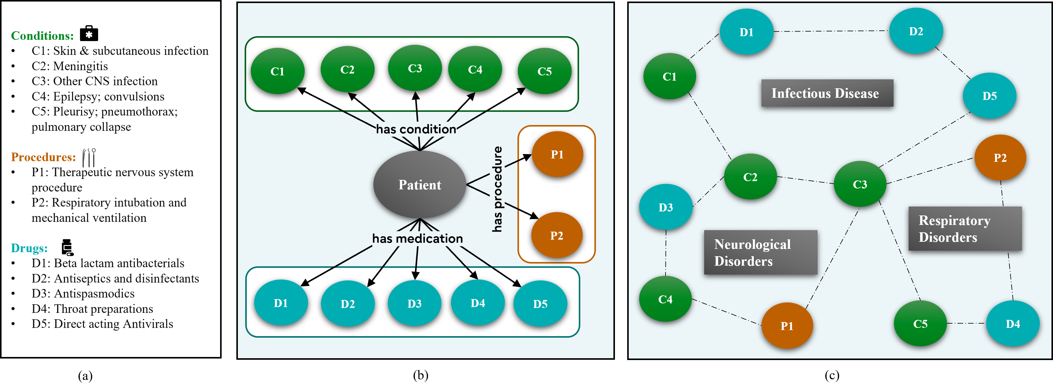
Knowledge Infused Hypergraph Construction: For each visit $t\in T_{i}$ of patient $P_{i}$, we construct a visit-level hypergraph to model higher-order clinical interactions through hyperedges that explicitly captures co-occurring conditions, medications, and procedures within a single visit. A naive approach would invoke a large language model (LLM) to construct a hypergraph independently for each visit. However, such a strategy incurs prohibitive token and computational costs. To address this limitation, we propose a cost-efficient two-stage procedure:

Stage 1: We first construct a global hyperknowledge graph (HKG) over the EHR concept vocabulary by aggregating unique clinical concepts across all patients. Using LLM prompting, we group semantically related conditions, medications, and procedures into clinically coherent concept sets. Each group defines a hyperedge, capturing meaningful higher-order clinical context. The HKG can be expanded by pooling information from external sources such as PubMed and UMLS along with the derived medical ontologies.

Stage 2: In the second step, the knowledge from global HKG is transferred to patient-specific hypergraph, instantiated for each visit, by selecting the subset of global hyperedges whose concepts are present in that visit. This approach of infusing knowledge into the hypergraph avoids repeated LLM calls, thus optimizing the compute and cost that accompanies use of LLM. To explicitly encode visit-level context, we introduce a dedicated visit node connected to all hyperedges in the corresponding hypergraph. Further details on the prompting strategy and construction are provided in Appendix C.1.

Formally, for a visit $t$ of patient $P_{i}$, we define a hypergraph as $\mathcal{H}_{i,t}=({\mathcal{V}}_{i,t},{\mathcal{E}}_{i,t})$, where $\mathcal{V}_{i,t}$ denotes the set of unique clinical entities appearing in $C_{i,t}$ and visit node, ${\mathcal{E}}_{i,t}=\{e_{i,t}^{(1)},e_{i,t}^{(2)},\ldots,e_{i,t}^{(K_{i,t})}\}$ is the set of hyperedges inferred by the LLM. A single visit can include multiple hyperedges, indicating that patient has multiple dissimilar concepts ($K_{i,t}$ for patient $i$). The hyperedge set is therefore a collection of unique concepts at time $t$ and is given by $\mathcal{E}_{i,t}=\bigcup_{k=1}^{K_{i,t}}e_{i,t}^{(k)}.$ The structure of this hypergraph is encoded by an incidence matrix $\mathbf{I}_{i,t}\in\mathbb{R}^{|\mathcal{V}_{i,t}|\times|\mathcal{E}_{i,t}|}$. Node features are initialized using BERT embeddings (devlin2019bertpretrainingdeepbidirectional) and projected to the latent space via a learnable linear layer.

Figure 2(c) illustrates a knowledge-infused hypergraph constructed from a single visit sample from the MIMIC-III dataset, with clinical concepts shown in Figure 2(a). In contrast, Figure 2(b) presents the corresponding pairwise KG, which models conditions, procedures, and medications independently despite their co-occurrence within the same visit. Consequently, it fails to capture the joint clinical context and interdependencies among factors such as neurological, infectious, and respiratory conditions. The knowledge-infused hypergraph addresses this limitation by encoding visit-level information through hyperedges that group clinically related concepts, enabling representation of higher-order disease patterns. For instance, in Figure 2(c), a hyperedge for respiratory disorders jointly connects pleurisy, respiratory intubation, mechanical ventilation, and associated medications. By modeling such multi-way interactions, the hypergraph provides a more expressive representation that supports richer clinical reasoning and improved downstream performance.

Knowledge Infused Temporal Hypergraphs. For each patient $P_{i}$, we construct a sequence of visit-level hypergraphs ordered by time i.e., $\mathcal{H}_{i}=\{\mathcal{H}_{i,1},\mathcal{H}_{i,2},\ldots,\mathcal{H}_{i,T_{i}}\}.$ This enables the proposed model to effectively capture the patient history as sequences of static hypergraphs. Further, this allows us to apply dynamic representation learning technique to exploit the temporal evolution.

In this section, we introduce proposed dynamic state-space model (SSM) over temporal hypergraphs.
Static Hypergraph Embedding. We first obtain static representations for each visit leveraging the corresponding hypergraph as an inductive bias for capturing higher-order clinical dependencies. Let $\mathbf{X}_{i,t}\in\mathbb{R}^{|\mathcal{V}_{i,t}|\times F}$, denote the feature matrix for patient $i$ at time $t$ with $F$ being feature dimension, and $\mathbf{I}_{i,t}\in\mathbb{R}^{|\mathcal{V}_{i,t}|\times|\mathcal{E}_{i,t}|}$ denote the hypergraph incidence matrix. We compute node embeddings $\mathbf{Z}_{i,t}\in\mathbb{R}^{|\mathcal{V}_{i,t}|\times d}$, using a hypergraph convolution operator (HConv) (bai2021hypergraph) as

where $\mathbf{Dv}_{i,t}\in\mathbb{R}^{|\mathcal{V}_{i,t}|\times|\mathcal{V}_{i,t}|}$ and $\mathbf{De}_{i,t}\in\mathbb{R}^{|\mathcal{E}_{i,t}|\times|\mathcal{E}_{i,t}|}$ denote the node and hyperedge degree matrices, respectively, $\mathbf{W}$ represents learnable hyperedge-specific weights, $\bm{\Theta}^{(l+1)}$ is the layer-specific trainable parameter matrix, and $\sigma(\cdot)$ is a non-linear activation function.

The update in Eq. (1) implements a spectral hypergraph convolution, generalizing graph convolution to higher-order relational structures. Message passing is performed via hyperedges, allowing information to be aggregated across groups of related clinical concepts. Further stacking multiple such hypergraph convolution layers, we obtain visit node embeddings that encode rich structural information from the static hypergraphs. These embeddings serve as inputs to temporal state-space model, which captures the temporal evolution of clinical states across visits.

Dynamic State-Space Model over Temporal Hypergraphs. The temporal hypergraphs associated with a patient is naturally represented as a sequence of static knowledge infused hypergraphs evolving over discrete time. We model this sequence as a discrete-time dynamic hypergraphs, enabling principled temporal representation learning over higher-order structures.

In particular for EHR data, clinically relevant signals may span long temporal horizons, necessitating framework for capturing long-range temporal information propagation. To address this, we adopt a state-space modeling (SSM) framework, which is well-suited for preserving and updating long-range temporal dependencies. Specifically, for a patient $P_{i}$ with sequence of hypergraphs as $\mathcal{H}_{i}=\{\mathcal{H}_{i,1},\mathcal{H}_{i,2},\ldots,\mathcal{H}_{i,T_{i}}\}$ the goal is to learn temporal latent representations $\mathbf{s}_{i}\in\mathbb{R}^{1\times f}$ that summarize the patient\CJK@punctchar\CJK@uniPunct0"80"99s clinical trajectory and support downstream prediction.

HiPPO-based Memory Representation. To model long-range temporal dependencies, we employ a Higher-Order Polynomial Projection Operator (HiPPO) framework (gu2020hippo). HiPPO-based models compress the entire history of inputs into a fixed-dimensional memory by maintaining coefficients of a polynomial basis, which are updated through a state-space formulation.

Let $k\in\{1,2,\ldots T_{i}\}$ index the discrete time clinical visits of patient $i$, with the $k$th visit at time instant $t_{k}$ and the interval between the visits as $\Delta_{k}=t_{k}-t_{k-1}$. Then the resulting discrete-time state-space update for patient $P_{i}$ (following T-SSM framework) is given by

where $\mathbf{A}\in\mathbb{R}^{f\times f}$, is a HiPPO matrix and $\tilde{\mathbf{x}}_{i,k}=\mathrm{HConv}_{v}(\mathbf{X}_{i,k},\mathcal{H}_{i,k})\mathbf{B}^{T}\in\mathbb{R}^{1\times f}$, represents the hypergraph-aware embeddings obtained via the hypergraph convolution operator defined in Eq. (1) with $\mathbf{B}\in\mathbb{R}^{f\times d}$ is a trainable input matrix. Importantly $\mathrm{HConv}_{v}(\mathbf{X}_{i,k},\mathcal{H}_{i,k})\in\mathbb{R}^{1\times d}$ output the visit node embedding by indexing the visit node in $\mathbf{Z}_{i,k}$. It can be observed from Eq. (2), the proposed model jointly captures higher-order spatial dependencies within individual visits and long-range temporal dependencies across visits due to SSM modeling. Thus the learned temporal representations are highly expressive and well-suited for downstream clinical tasks.

After processing the full visit sequence for patient $P_{i}$, the final output representation is obtained as $\mathbf{y}_{i}=\mathbf{C}\mathbf{s}_{i,K}^{T}$, where $\mathbf{s}_{i,K}$ denotes the memory representation after the final visit and $\mathbf{C}\in\mathbb{R}^{d_{1}\times f}$ is a learnable output matrix. Depending on the downstream task, the representation $\mathbf{y}_{i}$ is subsequently passed through a task-specific decoder to produce the final prediction.

In this section, we discuss the proposed method for extracting temporal reasoning paths. We discuss two variants based on attention and gradient-based attribution.
Attention based approach: To mitigate the challenges from HConv layer as discussed in Remark 3.1, we introduce an attention based hypergraph convolution (HGAT)(bai2021hypergraph) that assigns learnable importance weights to nodes and hyperedges, which can be subsequently leveraged to extract reasoning paths (ding2020more).

Let $v_{r}\in\mathcal{V}_{i,t}$ denote a vertex $r$ (clinical concept) of patient $i$ at visit $t$. To learn the representation of node $r$, the attention-based hypergraph convolution operates in two stages: (1) node to hyperedge aggregation, (2) hyperedge to node aggregation. In particular, the representation of node $r$ in layer $l$ i.e., $\mathbf{z}^{(l+1)}_{r}\in\mathbb{R}^{d\times 1}$ is obtained as

where $\mathcal{E}_{i,t}(v^{r})$ denotes set of hyperedges incident to node $v^{r}$, $e^{j}$ denotes $j^{th}$ hyperedge, $\hat{\mathbf{e}}^{(l+1)}_{j}$ is the updated representation of hyperedge $e^{j}$ (see Appendix C.2 for detailed derivation) and $\mathbf{W}^{(2)}\in\mathbb{R}^{d\times d}$ is a learnable weight matrix. $\beta_{r,j}$ is the hyperedge to node attention coefficient that quantifies the influence of hyperedge $e^{j}$ on node $v^{r}$. Here

$\mathbf{n}$ is a learnable vector and

$\tilde{\mathbf{h}}_{i,j}=\text{LeakyReLU}\left(\mathbf{W}^{(2)}\hat{\mathbf{e}}_{j}^{(l+1)}||\mathbf{W}^{(1)}\mathbf{z}^{(l)}_{r}\right).$ Learning the coefficients $\beta_{r,j}$ enables the model to explicitly identify the most influential hyperedges contributing to final representation. To extract interpretable reasoning paths, we sort the learned attention coefficients of visit node and select the top-$\omega$ concepts with the highest attention scores using $(\alpha,\,\beta)$. Further, these top-$\omega$ concepts are used to generate the temporal reasoning paths as detailed in the Appendix C.2.
Gradient based approach: While the attention-based approach introduced above enables fine-grained identification of important nodes and hyperedges, it requires learning both node- and edge-level attention weights and therefore incurs substantially higher parameter and computational complexity than the HConv operator. In resource constrained settings, we instead adopt a gradient based attribution strategy that directly leverages the embeddings produced by HConv, without introducing additional learnable parameters. Let $\mathbf{x}^{(j)}_{i,k}\in\mathbb{R}^{d}$ denote the embedding of clinical entity $j$ for patient $i$ at visit $k$. To quantify the contribution of this entity to the final prediction $\hat{y}_{i}$, we compute the gradient of $\hat{y}_{i}$ with respect to $\mathbf{x}^{(j)}_{i,k}$ i.e, $\nabla_{\mathbf{x}^{(j)}_{i,k}}\hat{y}_{i}$. This gradient reflects how changes in an entity\CJK@punctchar\CJK@uniPunct0"80"99s representation at a given visit propagate through the latent SSM dynamics and affect the final prediction.

Leveraging the gradients we then compute the saliency score (shrikumar2017learning) which accounts for feature presence and sensitivity. In particular the saliency score $Sc(e,k)$ for entity $j$ of patient $i$ at visit $k$ is given by $Sc(e,k)=\mathbf{x}^{(j)^{T}}_{i,k}\cdot\nabla_{\mathbf{x}^{(j)}_{i,k}}\hat{y}_{i}$.

A higher positive saliency score indicates that the corresponding clinical entity contributes more strongly toward increasing the outcome.

To translate saliency scores into an interpretable temporal reasoning path, we perform gradient-based backtracking using a set of anchors, defined as the top-$\omega$ entities in the final visit $K$ with the highest saliency scores. For each anchor, we reconstruct a reasoning path by tracing backward through time and selecting the entity at visit $k$ i.e., $e_{k}^{*}$ which maximizes the saliency score $Sc(e,k)$.

In Tables LABEL:tab:mortality, LABEL:tab:drug_rec, and LABEL:tab:los we present results (mean and standard deviation in brackets $(.)$) on three downstream clinical prediction tasks on the MIMIC-III and MIMIC-IV datasets. It can be observed that HoT-SSM demonstrates strong performance across all tasks compared to the baselines. In particular, it is important to notice that on mortality prediction, the proposed model achieves a improvement of +17.7% in AUPRC and +3.9% in AUROC over GraphCARE on the MIMIC-III dataset, asserting the importance of capturing higher-order relations for critical tasks. Whereas, on MIMIC-IV, we observe that the relative gains are much stronger with +17.1% in AUPRC and +11.6% in AUROC improvements compared to MIMIC-III, as the dataset includes patients with more visits, which showcases the ability of the model to capture long-range patient history. It can also be observed that the proposed model outperforms state-of-the-art algorithms on other clinical tasks, asserting the importance of hypergraphs and SSMs. Additional results on readmission prediction task are provided in Appendix E.3.

To study the impact of modeling higher-order clinical relationships with hypergraphs, we compare our proposed HoT-SSM framework against its graph-based counterpart, denoted as GNN-SSM. The latter models clinical relationships using knowledge graphs, similar to GraphCare (Graphcare). Table LABEL:graph_ssm reports the results on the mortality prediction task for both the MIMIC-III and MIMIC-IV datasets. As shown, HoT-SSM consistently outperforms GNN-SSM, demonstrating the advantage of explicitly modeling EHR data through hypergraphs.

To examine the impact of long-range temporal information propagation on predictive performance, we conduct an ablation study on a subset of patients with extended clinical histories (those with more than 10 recorded visits) with the mortality prediction task on the MIMIC-IV dataset. This setting is particularly challenging, as accurate prediction requires preserving clinically relevant information over long temporal horizons. We compare HoT-SSM against two architectural variants with SSM module is replaced by (i) Long Short-Term Memory (LSTM), (HoT-LSTM), and (ii) Hyper-GNN, which directly aggregates visit-level hypergraph representations without temporal modelling. In Table LABEL:tab:ablation_long_range, we report the results where it can be observed that HoT-SSM consistently outperforms both variants across all evaluation metrics. Notably, HoT-SSM achieves larger gains with +15% in Sensitivity and +6.5% in Macro-F1 score compared to the LSTM- baseline, thereby asserting the importance of proposed SSM framework for effectively capturing the long range clinical histories especially in critical tasks such as mortality prediction.

Further, to ensure that the observed gains are not solely due to LLM-based hyperedge construction, we investigate the following questions (see Appendix E.1).

• Q.1. How does HoT-SSM perform with non-LLM based hypergraph constructions? • Q.2. How robust and reliable are the performance gains?

The temporal reasoning module in the HoT-SSM pipeline extracts the reasoning paths by gradient or attention based methods. In Fig. 4, we present the reasoning path generated by gradient based approach that selects the top-2 most influential clinical entities per visit based on gradient contribution for a representative mortality case from the MIMIC-III dataset. Grounding the reasoning abilities to extracted reasoning chains we also show an LLM output explaining the reasons for models prediction towards high mortality risk. More examples on temporal reasoning paths are presented in Appendix F.