The BRUIT-FM "open data" noise reduction challenge
BRUIT-FM open data challenge \reporttypeData Report \creditConceptualizationCrawford, Ker, Rebeyrol \creditMethodologyCrawford, Ker, Rebeyrol \creditSoftwareCrawford \creditWriting - Original draftCrawford \creditWriting - Review & EditingKer, Duval
Abstract The BRUIT-FM Challenge asks participants to reduce "noise" on an open dataset of real and synthetic broadband seafloor seismology data. The dataset includes signals from earthquakes, ocean infragravity waves and seafloor currents. It also includes training datasets of synthetic data with solutions. Participants are asked to remove or separate these signals to obtain the best earthquake and seafloor compliance signals. The authors will make a first assessment of the noise reduction, based on noise reduction and ease of use. Participants are invited to a community workshop, in which they will validate the preliminary assessment and collaborate on a community paper describing the results, identifying promising pathways and proposing new directions. The best results will be added to a new version of the dataset, which will persist as a benchmark for future developments.
1 Introduction
Seafloor seismology measurements are needed to study the structure and dynamics of Earth features that are beneath or near oceans and seas (i.e. subduction zones, mid-ocean ridges, intraplate volcanos, and coastal fault zones) and to properly cover the earth for global seismology studies. The ocean layer over the measurement stations affects the seismology signal (e.g. (Ruan et al. 2014; Blackman et al. 1995)) and creates new signals — such as the motion under pressure from ocean waves ((Yamamoto 1983; Crawford et al. 1991)) and the tilt generated by seafloor currents (e.g. (Crawford and Webb 2000)). To best use any of these signals, the other signals should be separated or reduced (e.g. (Duennebier and Sutton 1995; Webb and Crawford 1999; Crawford and Webb 2000; Janiszewski et al. 2023)). Several computational toolboxes have been created to reduce seafloor noise, primarily at frequencies below the microseism peak (< 0.03 Hz). Most of them are based on the calculation of the transfer function with another channel that contains a stronger version of the noise signal (e.g. Janiszewski et al. 2019; Crawford and Webb 2000; Rebeyrol et al. 2024; Aminian et al. 2025), but there are also methods using music theory (Zali et al. 2023) and re-orientation of the vertical channel (Harmon et al. 2022). Marine seismologists are thus confronted by an array of tools, without knowing which is the best for their given problem, because neither efficiency of each method, nor the potential for them to deform the target signal, has been objectively evaluated.
We have created a dataset and a protocol to evaluate the efficiency of noise reduction techniques and toolboxes. Our goal is to identify which existing techniques work the best and how new techniques might allow us to further improve noise reduction.
The dataset consists of two "challenge" data files ("validation", in machine learning language) and a large number of "training" data files and responses ("calibration"). We ask participants to run their algorithms on the challenge datasets and to return "cleaned" datasets and/or a calculated seafloor compliance (pressure/acceleration ratio in the absence of earthquakes (Crawford et al. 1998)) to the following address: bruitfm_challenge@services.cnrs.fr. For scientists who are not used to seafloor seismology datasets but who have source separation algorithms that they think may be efficient, we also provide sample codes for reading and writing the files and we allow compliance to be returned in its "raw" (digital data values) format, without taking into account the instrument response.
We will first collect the answers that were generated using different techniques and compare the outputs using three criteria: 1) noise reduction, 2) deformation of the desired signal, and 3) ease of use. Noise reduction will be calculated using the variance of the cleaned signal at frequencies beneath the microseism band, and the area of the pressure-vertical coherence at frequencies beneath the microseism band. Deformation will be calculated for the synthetic challenge data, by comparing the cleaned signal and compliance to their input values. Ease of use will be calculated based on 1) code clarity, 2) code brevity and 3) the number of manually-set parameters needed to obtain the provided results. We will then collate the responses and organize a workshop to verify our classification, discuss the advantages and disadvantages of each method, and write a community paper on the results. All "successful" codes and datasets will be integrated into the open dataset, to allow future tests of new techniques.
2 The Datasets
The datasets are available at Crawford et al. 2025. There are two challenge datasets, one using real data (8 days) and the other using synthetic data (10 days). There are also one main (10-day) and 100 "mass" (1-day) training datasets. Each training dataset includes answer files with the best outputs.
2.1 Data format and sampling rate
The data are stored in miniSEED files with four channels named: \codeLDH or \codeLDG for the pressure component, \codeLH1 and \codeLH2 for the horizontal seismometer components, and \codeLHZ for the vertical seismometer component. The sampling rate is 1 sample per second. Provided example scripts show how to read the data and write the outputs.
2.2 Synthetic Data
Synthetic data allows us to generate reference answer files that can be used to evaluate results. They are constructed using a combination of 1) real seismological data from a quiet land station and 2) synthetic seafloor noise data constructed using the \codeSeafloorSynthetic class of the \codetiskitpy software module (Crawford 2025).
The \codeSeafloorSynthetic class simulates seafloor noise as a combination of (Fig. 1):
- 1.
Instrumental noise floors for the seismometer and pressure sensors;
- 2.
The infragravity (low frequency) wave surface height;
- 3.
A 1D model of earth structure beneath the seafloor station;
- 4.
The misalignment of the seismometer’s vertical channel from gravitational vertical;
- 5.
The maximum seismometer tilt noise levels at the seafloor;
- 6.
The direction of the tilt noise with respect to the seismometer;
- 7.
The number of decibels below the maximum tilt noise levels for minimum tilt levels; and
- 8.
The water depth.
It does not include the ocean wind wave surface spectrum or microseisms, which are important at higher frequencies and/or shallow (<500m) water depth. It does not model temporal variations in the infragravity wave energy, nor in the seismometer’s misalignment. The class generates seafloor pressure and acceleration signals from the parameters, varying the tilt noise over time in rhythm with the tides.

2.3 Challenge Datasets
2.3.1 Real Data
The real data are from a seafloor station with high local seismicity and a relatively small compliance signal. An example of the outputs obtainable using the \codetiskitpy module is provided with the dataset and shown in subsection 4.1.
2.3.2 Synthetic Data
The synthetic data are a 10-day dataset that sums 1) a synthetic noise model with unspecified noise parameters; and 2) real waveforms including significant global earthququakes, recorded on an unidentified quiet broadband land station. The start date is set to 2024-01-01 so that the earthquakes do not correspond to their actual dates.
2.4 Training Datasets
2.4.1 Main dataset
The main training dataset is generated by the same process as the synthetic challenge dataset, except with different noise parameters and a different record of high global seismicity recorded on a quiet land station. "Answer" files are provided.
2.4.2 Mass datasets
The mass training dataset consists of 100 synthetic data files and their answer data and compliance files. The synthetic data are generated in the same way as for the synthetic challenge and main training waveforms, with noise parameters and the time period of the land data randomly selected. The land station data for half of the mass datasets includes a global earthquake with a reported magnitude greater than or equal to 5.2.
3 Seafloor compliance
For the purposes of this challenge, seafloor compliance is the ratio of the vertical seafloor motion to the pressure signal, at frequencies where the two are coherent. "Cleaned for compliance" data are data from which all noise sources that reduce the pressure-vertical coherence have been removed/minimized. Compliance can be returned either in units of the digital data or in Pa-1: the latter requires using instrument response and water depth information from the inventory file. More details on seafloor compliance can be found in Yamamoto 1983; Crawford et al. 1991; Crawford et al. 1998; Aminian et al. 2025.
4 The noise reduction challenge
Participants should download the dataset from the Zenodo repository (Crawford et al. 2025). They should apply their noise reduction codes to the challenge datasets and create one or more of the following files:
- 1.
Waveform data cleaned of everything except earthquakes ("clean_for_eq");
- 2.
Waveform data cleaned of everything except seafloor compliance ("clean_for_compl");
- 3.
Seafloor compliance, in units of data (COUNTS) or Pa-1;
- 4.
Source code or an explanation of the algorithms used.
File names and formats are specified in section 5.2, examples are provided in the repository’s \codeTRAINING/ subdirectories, and example codes to produce them are provided in the repository’s \codeCODES/ directory. Responses should be sent to bruitfm_challenge@services.cnrs.fr.
No knowledge of seismological processing is needed. The data are in a seismological standard format (miniSEED), but example code is provided (using the open source \codeobspy (Beyreuther et al. 2010) software) to read and display the data in a python environment. Each directory contains an "inventory" file in StationXML format, which is only needed if the participant chooses to return the compliance in units of Pa-1.
4.1 An example of cleaning the main training dataset
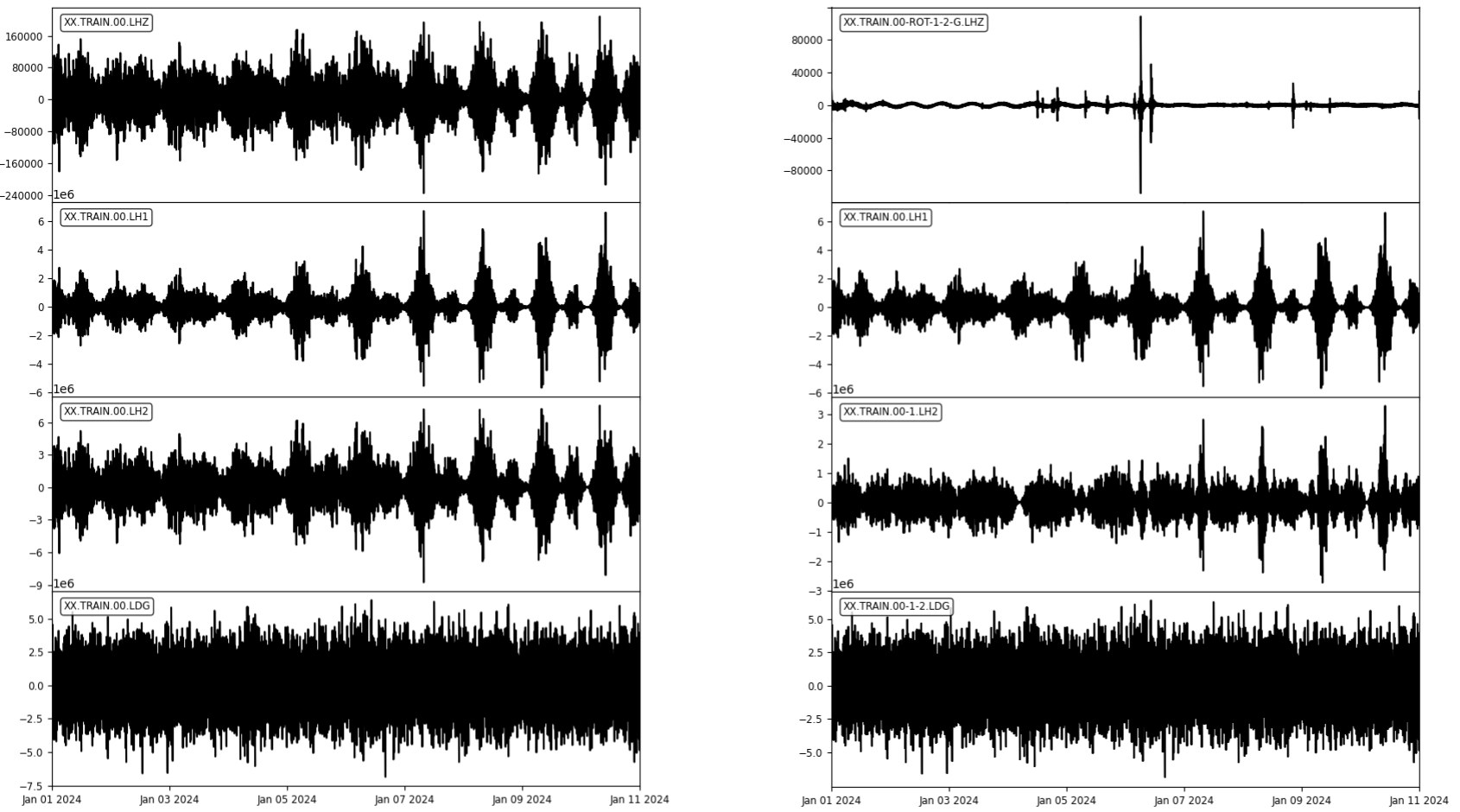
We show below the results of the repository’s example code \codeCODES/3_read_write_clean_tiskitpy.py, which reads in the main training dataset, cleans it using \codetiskitpy, and outputs the results. \codetiskitpy is just one of several modules to clean data and it is not needed to process the data: the point of this example is to demonstrate one approach to reading and cleaning the data and preparing the output files. After reading the data and metadata, the program plots the data, rotates the vertical channel to minimize noise on that channel, then calculates cleaning functions based on transfer functions with 1) the horizontal channels ("clean for compliance"); and 2) the horizontal and pressure channels ("clean"). It plots the original data and the cleaned waveforms (Fig. 2), then the power spectral densities for all levels of cleaning (Fig: 3) and writes the "clean" data to a miniSEED file and the compliance calculation to a CSV file.

Below is the section of the code for reading the input files:
The code generates "cleaned for earthquakes" data (\codestream_rot_12G), "cleaned for compliance" data (\codestream_rot_12) and compliance (\codencompl_calcd). Below is the section of the code for writing these out:
ncompl_calcd is a \codetiskitpy object with its own “write()“ method. Other example codes show how to write the compliance output file without using \codetiskitpy.
4.2 An example of cleaning the "real" challenge dataset
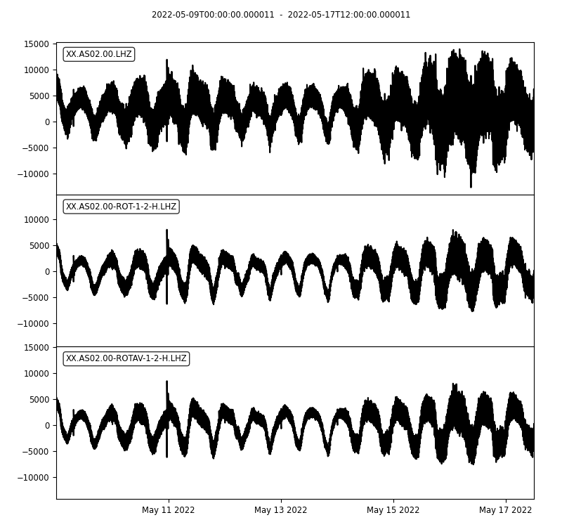
Below are the results of the example code \codeCODE/4_clean_avoid_tiskitpy.py, which reads in the \codeREAL/ challenge dataset and cleans it using \codetiskitpy, both automatically and with manual selection of which windows to use for the noise calculations. Fig. 4 shows waveforms for the original and cleaned data, while Fig: 5 shows PSDs and coherences for these waveforms. There is little visible difference between the automatic and manual window selection in the waveform plots, but the pressure-vertical coherence is significantly better for the manual window selection, allowing a more precise compliance calculation.

Acknowledgements.
This project is funded by the French national research agency (ANR) BRUIT-FM project (ANR-21-CE01-0031). We thank Guilhem Barruol and Eleonore Stutzmann for project coordination and useful discussions. We also thank Xongbo Zu for his input on microseism modeling, which should be included in a future version of \codetiskitpy.Data and code availability
The data are available at (Crawford et al. 2025). The \codetiskitpy package is available at (Crawford 2025) or can be installed using the Python Package Index (command line: \codepip install tiskitpy).
Competing interests
The authors have no competing interests.
5 Supplementary Information
5.1 Directory structure
The files are organized as follows:
- •
\code
CHALLENGE/: contains the challenge datasets, one data file and one metadata files per directory
- –
\code
REAL/: a real seafloor dataset
- –
\code
SYNTHETIC/: a synthetic seafloor dataset
- –
- •
\code
CODES/: example codes for reading the data and writing the output files
- •
\code
TRAINING/: Training datasets. Each dataset includes a data file, a metadata file, and "correct" answer files (one data, one compliance in COUNTS/COUNTS, one compliance in Pa-1). All of the data files are synthetic.
- –
\code
MAIN/: One 10-day training dataset.
- –
\code
MASS/: One hundred 1-day training datasets and answers.
- –
The \codeMAIN training data set contains the input files \codeTRAIN_noisy.mseed, \codeTRAIN_inv.xml) and the answer files \codeTRAIN_clean.mseed, \codeTRAIN_clean_compl.mseed, \codeTRAIN_compliance_COUNTS.csv and \codeTRAIN_compliance_Pa-1.csv). The \codeMASS training data set contains one metadata file, (\codeMASS_inv.xml), 100 data files (\codeMASSxxx_noisy.mseed) and 100 each answer files (\codeMASSxxx_clean.mseed, \codeMASSxxx_clean_compl.mseed\codeMASSxxx_compliance_COUNTS.csv and \codeMASSxxx_compliance_Pa-1.csv), where \codexxx is a number from \code000 to \code099.
5.2 File formats and names
5.2.1 Data files
Input data files are in miniSEED format and are named \code{SOMETHING}_noisy.mseed.
Output data files should be in miniSEED format, use the same channel names as the input files, and be named \code{SOMETHING}_clean_for_eq.mseed if cleaned of everything except earthquakes and \code{SOMETHING}_clean_for_compl.mseed if cleaned for compliance.
5.2.2 Inventory files
Inventory files are in StationXML format and are named \code{SOMETHING}_inv.xml.
5.2.3 Compliance files
Compliance values should be stored in CSV format and named \code{SOMETHING}_compliance_COUNTS.csv if the units are the values in the data file, or \code{SOMETHING}_compliance_Pa-1.csv if they have been transformed to physical units. The file should have a first line with the fixed headers shown in Listing 3, followed by as many lines as there are frequencies at which compliance was calculated. Frequencies are in Hz, compliance and uncertainty are in the appropriate units for the filename (COUNTS/COUNTS or Pa-1) and phase is in degrees. The ‘coherence‘ column may be omitted or left empty Lines starting with \code# are considered comments and ignored.
5.2.4 Codes and/or algorithms
Codes and/or algorithms should be text files with appropriate suffixes (e.g., .txt, .md, .py, .cpp, …). If there are several files, please include a \codeREADME.txt or \codeREADME.md file explaining each file.
5.3 Example Codes
The \codeCODE/ directory contains example codes of increasing complexity:
- \code0_read_write.py
-
Read in and write out miniseed data and "raw" compliance (no need for the inventory file).
- \code1_read_write_inv.py
-
Read in and write out miniseed data and "normalized" compliance (uses the inventory file).
- \code2_read_write_tiskitpy.py
-
Read in and write out miniseed data and "normalized" compliance. Use \codetiskitpy (Crawford 2025) to plot power spectral densities and coherences, and to write out the compliance.
- \code3_read_write_clean_tiskitpy.py
-
Read in the main training dataset and write out miniseed data and normalized compliance, using \codetiskitpy with automatically-selected timespans (removes USGS-catalogue earthquakes and "outlier" windows)
- \code4_clean_avoid_tiskitpy.py
-
Read in the "real" challenge dataset and write out miniseed data and normalized compliance , using \codetiskitpy with manually-selected timespans.
References
- Aminian et al. (2025) Aminian, M. A., Crawford, W., Stutzmann, E., Montagner, J.-P., Cannat, M., and Hadziioannou, C. Shallow Crustal Structures of the Indian Ocean Derived from Compliance Function Analysis. Geophys. J. Int., 242:1–16, 2025. 10.1093/gji/ggaf253.
- Beyreuther et al. (2010) Beyreuther, M., Barsch, R., Krischer, L., Megies, T., Behr, Y., and Wassermann, J. ObsPy: A Python Toolbox for Seismology. Seis. Res. Lett., 81(3):530–533, 2010. 10.1785/gssrl.81.3.530.
- Blackman et al. (1995) Blackman, D. K., Orcutt, J. A., and Forsyth, D. W. Recording teleseismic earthquakes using ocean-bottom seismographs at mid-ocean ridges. Bull. Seis. Soc. Am., 85(6):1648–1664, 1995. 10.1785/BSSA0850061648.
- Crawford et al. (2025) Crawford, W., Rebeyrol, S., and Ker, S. BRUIT-FM challenge dataset, September 16 2025. 10.5281/zenodo.17132828.
- Crawford (2025) Crawford, W. C. tiskitpy: TIme Series toolKIT, October 9 2025. 10.5281/zenodo.17305413.
- Crawford and Webb (2000) Crawford, W. C. and Webb, S. C. Removing tilt noise from low frequency (<0.1 Hz) seafloor vertical seismic data. Bull. Seis. Soc. Am., 90(4):952–963, 2000. 10.1785/0119990121.
- Crawford et al. (1991) Crawford, W. C., Webb, S. C., and Hildebrand, J. A. Seafloor compliance observed by long-period pressure and displacement measurements. J. Geophys. Res., 96(10):16151–16160, 1991. 10.1029/91JB01577.
- Crawford et al. (1998) Crawford, W. C., Webb, S. C., and Hildebrand, J. A. Estimating shear velocities in the oceanic crust from compliance measurements by two-dimensional finite difference modeling. J. Geophys. Res., 103(5):9895–9916, 1998. 10.1029/97JB03532.
- Duennebier and Sutton (1995) Duennebier, F. K. and Sutton, G. H. Fidelity of ocean bottom seismic observations. Mar. Geophys. Res., 17:535–555, 1995. 10.1007/BF01204343.
- Harmon et al. (2022) Harmon, N., Laske, G., Crawford, W., and Rychert, C. Tilt Corrections for Normal Mode Observations on Ocean Bottom Seismic Data, an example from the PI-LAB experiment. Seismica, 1, 2022. 10.26443/seismica.v1i1.196.
- Janiszewski et al. (2019) Janiszewski, H. A., Gaherty, J. B., Abers, G. A., Gao, H., and Eilon, Z. C. Amphibious surface-wave phase-velocity measurements of the Cascadia subduction zone. Geophys. J. Int., 217(3):1929–1948, 2019. 10.1093/gji/ggz051.
- Janiszewski et al. (2023) Janiszewski, H. A., Eilon, Z., Russell, J. B., Brunsvik, B., Gaherty, J. B., Mosher, S. G., Hawley, W. B., and Coats, S. Broad-band ocean bottom seismometer noise properties. Geophys. J. Int., 233(1):297–315, 2023. 10.1093/gji/ggac450.
- Rebeyrol et al. (2024) Rebeyrol, S., Ker, S., Duval, L., and Crawford, W. C. Revisiting the OBS seafloor compliance signal removal with a stationarity and stacking-based approach: the BRUIT-FM toolbox. Geophys. J. Int., 239(1):386–401, 2024. 10.1093/gji/ggae265.
- Ruan et al. (2014) Ruan, Y., Forsyth, D., and Bell, S. Marine sediment shear velocity structure from the ratio of displacement to pressure of Rayleigh waves at seafloor. J. Geophys. Res. Solid Earth, 119:6357–6371, 2014. 10.1002/2014JB011162.
- Webb and Crawford (1999) Webb, S. C. and Crawford, W. C. Long period seafloor seismology and deformation under ocean waves. Bull. Seis. Soc. Am., 89(6):1535–1542, 1999. 10.1785/BSSA0890061535.
- Yamamoto (1983) Yamamoto, T. Propagator matrix for continuously layered porous seabeds. Bull. Seis. Soc. Am., 73(6):1599–1620, 1983.
- Zali et al. (2023) Zali, Z., Rein, T., Krüger, F., Ohrnberger, M., and Scherbaum, F. Ocean bottom seismometer (OBS) noise reduction from horizontal and vertical components using harmonic–percussive separation algorithms. Solid Earth, 14(2):181–195, 2023. 10.5194/se-14-181-2023.
